Welcome message from author
This document is posted to help you gain knowledge. Please leave a comment to let me know what you think about it! Share it to your friends and learn new things together.
Transcript
IN THIS CHAPTERYOU WILL . . .
Discuss howincent ives a f fectpeop le ’s behav ior
Learn the meaning o foppor tun i ty cost
Learn thateconomics is about
the a l locat ion o fscarce r esources
Examine some o f thet radeof fs that peop le
face
See how to usemarg ina l r eason ing
when makingdec is ions
The word economy comes from the Greek word for “one who manages a house-hold.” At first, this origin might seem peculiar. But, in fact, households andeconomies have much in common.
A household faces many decisions. It must decide which members of thehousehold do which tasks and what each member gets in return: Who cooks din-ner? Who does the laundry? Who gets the extra dessert at dinner? Who gets tochoose what TV show to watch? In short, the household must allocate its scarce re-sources among its various members, taking into account each member’s abilities,efforts, and desires.
Like a household, a society faces many decisions. A society must decide whatjobs will be done and who will do them. It needs some people to grow food, otherpeople to make clothing, and still others to design computer software. Once soci-ety has allocated people (as well as land, buildings, and machines) to various jobs,
T E N P R I N C I P L E S
O F E C O N O M I C S
3
Cons ider why t radeamong peop le or
nat ions can be goodfor ever yone
Discuss why marketsare a good, but not
per fect , way toa l locate r esources
Learn whatdetermines some
trends in the overa l leconomy
1
1
TLFeBOOK
4 PART ONE INTRODUCTION
it must also allocate the output of goods and services that they produce. It mustdecide who will eat caviar and who will eat potatoes. It must decide who willdrive a Porsche and who will take the bus.
The management of society’s resources is important because resources arescarce. Scarcity means that society has limited resources and therefore cannot pro-duce all the goods and services people wish to have. Just as a household cannotgive every member everything he or she wants, a society cannot give every indi-vidual the highest standard of living to which he or she might aspire.
Economics is the study of how society manages its scarce resources. In mostsocieties, resources are allocated not by a single central planner but through thecombined actions of millions of households and firms. Economists therefore studyhow people make decisions: how much they work, what they buy, how much theysave, and how they invest their savings. Economists also study how people inter-act with one another. For instance, they examine how the multitude of buyers andsellers of a good together determine the price at which the good is sold and thequantity that is sold. Finally, economists analyze forces and trends that affectthe economy as a whole, including the growth in average income, the fraction ofthe population that cannot find work, and the rate at which prices are rising.
Although the study of economics has many facets, the field is unified by sev-eral central ideas. In the rest of this chapter, we look at Ten Principles of Economics.These principles recur throughout this book and are introduced here to give youan overview of what economics is all about. You can think of this chapter as a “pre-view of coming attractions.”
HOW PEOPLE MAKE DECISIONS
There is no mystery to what an “economy” is. Whether we are talking about theeconomy of Los Angeles, of the United States, or of the whole world, an economyis just a group of people interacting with one another as they go about their lives.Because the behavior of an economy reflects the behavior of the individuals whomake up the economy, we start our study of economics with four principles of in-dividual decisionmaking.
PRINCIPLE #1: PEOPLE FACE TRADEOFFS
The first lesson about making decisions is summarized in the adage: “There is nosuch thing as a free lunch.” To get one thing that we like, we usually have to giveup another thing that we like. Making decisions requires trading off one goalagainst another.
Consider a student who must decide how to allocate her most valuable re-source—her time. She can spend all of her time studying economics; she can spendall of her time studying psychology; or she can divide her time between the twofields. For every hour she studies one subject, she gives up an hour she could haveused studying the other. And for every hour she spends studying, she gives up anhour that she could have spent napping, bike riding, watching TV, or working ather part-time job for some extra spending money.
scarc i tythe limited nature of society’sresources
economicsthe study of how society manages itsscarce resources
2 Ten Principles of Economics
TLFeBOOK
CHAPTER 1 TEN PRINCIPLES OF ECONOMICS 5
Or consider parents deciding how to spend their family income. They can buyfood, clothing, or a family vacation. Or they can save some of the family incomefor retirement or the children’s college education. When they choose to spend anextra dollar on one of these goods, they have one less dollar to spend on someother good.
When people are grouped into societies, they face different kinds of tradeoffs.The classic tradeoff is between “guns and butter.” The more we spend on nationaldefense to protect our shores from foreign aggressors (guns), the less we can spendon consumer goods to raise our standard of living at home (butter). Also importantin modern society is the tradeoff between a clean environment and a high level ofincome. Laws that require firms to reduce pollution raise the cost of producinggoods and services. Because of the higher costs, these firms end up earning smallerprofits, paying lower wages, charging higher prices, or some combination of thesethree. Thus, while pollution regulations give us the benefit of a cleaner environ-ment and the improved health that comes with it, they have the cost of reducingthe incomes of the firms’ owners, workers, and customers.
Another tradeoff society faces is between efficiency and equity. Efficiencymeans that society is getting the most it can from its scarce resources. Equitymeans that the benefits of those resources are distributed fairly among society’smembers. In other words, efficiency refers to the size of the economic pie, andequity refers to how the pie is divided. Often, when government policies are beingdesigned, these two goals conflict.
Consider, for instance, policies aimed at achieving a more equal distribution ofeconomic well-being. Some of these policies, such as the welfare system or unem-ployment insurance, try to help those members of society who are most in need.Others, such as the individual income tax, ask the financially successful to con-tribute more than others to support the government. Although these policies havethe benefit of achieving greater equity, they have a cost in terms of reduced effi-ciency. When the government redistributes income from the rich to the poor, it re-duces the reward for working hard; as a result, people work less and producefewer goods and services. In other words, when the government tries to cut theeconomic pie into more equal slices, the pie gets smaller.
Recognizing that people face tradeoffs does not by itself tell us what decisionsthey will or should make. A student should not abandon the study of psychologyjust because doing so would increase the time available for the study of econom-ics. Society should not stop protecting the environment just because environmen-tal regulations reduce our material standard of living. The poor should not beignored just because helping them distorts work incentives. Nonetheless, ac-knowledging life’s tradeoffs is important because people are likely to make gooddecisions only if they understand the options that they have available.
PRINCIPLE #2: THE COST OF SOMETHING ISWHAT YOU GIVE UP TO GET IT
Because people face tradeoffs, making decisions requires comparing the costs andbenefits of alternative courses of action. In many cases, however, the cost of someaction is not as obvious as it might first appear.
Consider, for example, the decision whether to go to college. The benefit is in-tellectual enrichment and a lifetime of better job opportunities. But what is thecost? To answer this question, you might be tempted to add up the money you
ef f ic iencythe property of society getting themost it can from its scarce resources
equ i tythe property of distributing economicprosperity fairly among the membersof society
Ten Principles of Economics 3
TLFeBOOK
6 PART ONE INTRODUCTION
spend on tuition, books, room, and board. Yet this total does not truly representwhat you give up to spend a year in college.
The first problem with this answer is that it includes some things that are notreally costs of going to college. Even if you quit school, you would need a place tosleep and food to eat. Room and board are costs of going to college only to the ex-tent that they are more expensive at college than elsewhere. Indeed, the cost ofroom and board at your school might be less than the rent and food expenses thatyou would pay living on your own. In this case, the savings on room and boardare a benefit of going to college.
The second problem with this calculation of costs is that it ignores the largestcost of going to college—your time. When you spend a year listening to lectures,reading textbooks, and writing papers, you cannot spend that time working at ajob. For most students, the wages given up to attend school are the largest singlecost of their education.
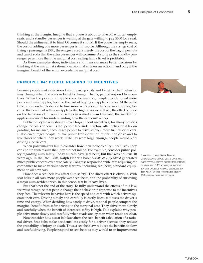
The opportunity cost of an item is what you give up to get that item. Whenmaking any decision, such as whether to attend college, decisionmakers should beaware of the opportunity costs that accompany each possible action. In fact, theyusually are. College-age athletes who can earn millions if they drop out of schooland play professional sports are well aware that their opportunity cost of collegeis very high. It is not surprising that they often decide that the benefit is not worththe cost.
PRINCIPLE #3: RATIONAL PEOPLE THINK AT THE MARGIN
Decisions in life are rarely black and white but usually involve shades of gray.When it’s time for dinner, the decision you face is not between fasting or eatinglike a pig, but whether to take that extra spoonful of mashed potatoes. When ex-ams roll around, your decision is not between blowing them off or studying 24hours a day, but whether to spend an extra hour reviewing your notes instead ofwatching TV. Economists use the term marginal changes to describe small incre-mental adjustments to an existing plan of action. Keep in mind that “margin”means “edge,” so marginal changes are adjustments around the edges of what youare doing.
In many situations, people make the best decisions by thinking at the margin.Suppose, for instance, that you asked a friend for advice about how many years tostay in school. If he were to compare for you the lifestyle of a person with a Ph.D.to that of a grade school dropout, you might complain that this comparison is nothelpful for your decision. You have some education already and most likely aredeciding whether to spend an extra year or two in school. To make this decision,you need to know the additional benefits that an extra year in school would offer(higher wages throughout life and the sheer joy of learning) and the additionalcosts that you would incur (tuition and the forgone wages while you’re in school).By comparing these marginal benefits and marginal costs, you can evaluate whetherthe extra year is worthwhile.
As another example, consider an airline deciding how much to charge passen-gers who fly standby. Suppose that flying a 200-seat plane across the country coststhe airline $100,000. In this case, the average cost of each seat is $100,000/200,which is $500. One might be tempted to conclude that the airline should neversell a ticket for less than $500. In fact, however, the airline can raise its profits by
oppor tun i ty costwhatever must be given up to obtainsome item
marg ina l changessmall incremental adjustments to aplan of action
4 Ten Principles of Economics
TLFeBOOK
CHAPTER 1 TEN PRINCIPLES OF ECONOMICS 7
thinking at the margin. Imagine that a plane is about to take off with ten emptyseats, and a standby passenger is waiting at the gate willing to pay $300 for a seat.Should the airline sell it to him? Of course it should. If the plane has empty seats,the cost of adding one more passenger is minuscule. Although the average cost offlying a passenger is $500, the marginal cost is merely the cost of the bag of peanutsand can of soda that the extra passenger will consume. As long as the standby pas-senger pays more than the marginal cost, selling him a ticket is profitable.
As these examples show, individuals and firms can make better decisions bythinking at the margin. A rational decisionmaker takes an action if and only if themarginal benefit of the action exceeds the marginal cost.
PRINCIPLE #4: PEOPLE RESPOND TO INCENTIVES
Because people make decisions by comparing costs and benefits, their behaviormay change when the costs or benefits change. That is, people respond to incen-tives. When the price of an apple rises, for instance, people decide to eat morepears and fewer apples, because the cost of buying an apple is higher. At the sametime, apple orchards decide to hire more workers and harvest more apples, be-cause the benefit of selling an apple is also higher. As we will see, the effect of priceon the behavior of buyers and sellers in a market—in this case, the market forapples—is crucial for understanding how the economy works.
Public policymakers should never forget about incentives, for many policieschange the costs or benefits that people face and, therefore, alter behavior. A tax ongasoline, for instance, encourages people to drive smaller, more fuel-efficient cars.It also encourages people to take public transportation rather than drive and tolive closer to where they work. If the tax were large enough, people would startdriving electric cars.
When policymakers fail to consider how their policies affect incentives, theycan end up with results that they did not intend. For example, consider public pol-icy regarding auto safety. Today all cars have seat belts, but that was not true 40years ago. In the late 1960s, Ralph Nader’s book Unsafe at Any Speed generatedmuch public concern over auto safety. Congress responded with laws requiring carcompanies to make various safety features, including seat belts, standard equip-ment on all new cars.
How does a seat belt law affect auto safety? The direct effect is obvious. Withseat belts in all cars, more people wear seat belts, and the probability of survivinga major auto accident rises. In this sense, seat belts save lives.
But that’s not the end of the story. To fully understand the effects of this law,we must recognize that people change their behavior in response to the incentivesthey face. The relevant behavior here is the speed and care with which drivers op-erate their cars. Driving slowly and carefully is costly because it uses the driver’stime and energy. When deciding how safely to drive, rational people compare themarginal benefit from safer driving to the marginal cost. They drive more slowlyand carefully when the benefit of increased safety is high. This explains why peo-ple drive more slowly and carefully when roads are icy than when roads are clear.
Now consider how a seat belt law alters the cost–benefit calculation of a ratio-nal driver. Seat belts make accidents less costly for a driver because they reducethe probability of injury or death. Thus, a seat belt law reduces the benefits to slowand careful driving. People respond to seat belts as they would to an improvement
BASKETBALL STAR KOBE BRYANT
UNDERSTANDS OPPORTUNITY COST AND
INCENTIVES. DESPITE GOOD HIGH SCHOOL
GRADES AND SAT SCORES, HE DECIDED
TO SKIP COLLEGE AND GO STRAIGHT TO
THE NBA, WHERE HE EARNED ABOUT
$10 MILLION OVER FOUR YEARS.
Ten Principles of Economics 5
TLFeBOOK
8 PART ONE INTRODUCTION
in road conditions—by faster and less careful driving. The end result of a seat beltlaw, therefore, is a larger number of accidents.
How does the law affect the number of deaths from driving? Drivers whowear their seat belts are more likely to survive any given accident, but they are alsomore likely to find themselves in an accident. The net effect is ambiguous. More-over, the reduction in safe driving has an adverse impact on pedestrians (and ondrivers who do not wear their seat belts). They are put in jeopardy by the law be-cause they are more likely to find themselves in an accident but are not protectedby a seat belt. Thus, a seat belt law tends to increase the number of pedestriandeaths.
At first, this discussion of incentives and seat belts might seem like idle spec-ulation. Yet, in a 1975 study, economist Sam Peltzman showed that the auto-safetylaws have, in fact, had many of these effects. According to Peltzman’s evidence,these laws produce both fewer deaths per accident and more accidents. The net re-sult is little change in the number of driver deaths and an increase in the numberof pedestrian deaths.
Peltzman’s analysis of auto safety is an example of the general principle thatpeople respond to incentives. Many incentives that economists study are morestraightforward than those of the auto-safety laws. No one is surprised that peopledrive smaller cars in Europe, where gasoline taxes are high, than in the UnitedStates, where gasoline taxes are low. Yet, as the seat belt example shows, policiescan have effects that are not obvious in advance. When analyzing any policy, wemust consider not only the direct effects but also the indirect effects that workthrough incentives. If the policy changes incentives, it will cause people to altertheir behavior.
QUICK QUIZ: List and briefly explain the four principles of individual decisionmaking.
HOW PEOPLE INTERACT
The first four principles discussed how individuals make decisions. As wego about our lives, many of our decisions affect not only ourselves but otherpeople as well. The next three principles concern how people interact with oneanother.
PRINCIPLE #5: TRADE CAN MAKE EVERYONE BETTER OFF
You have probably heard on the news that the Japanese are our competitors in theworld economy. In some ways, this is true, for American and Japanese firms doproduce many of the same goods. Ford and Toyota compete for the same cus-tomers in the market for automobiles. Compaq and Toshiba compete for the samecustomers in the market for personal computers.
Yet it is easy to be misled when thinking about competition among countries.Trade between the United States and Japan is not like a sports contest, where one
6 Ten Principles of Economics
TLFeBOOK
CHAPTER 1 TEN PRINCIPLES OF ECONOMICS 9
side wins and the other side loses. In fact, the opposite is true: Trade between twocountries can make each country better off.
To see why, consider how trade affects your family. When a member of yourfamily looks for a job, he or she competes against members of other families whoare looking for jobs. Families also compete against one another when they goshopping, because each family wants to buy the best goods at the lowest prices. So,in a sense, each family in the economy is competing with all other families.
Despite this competition, your family would not be better off isolating itselffrom all other families. If it did, your family would need to grow its own food,make its own clothes, and build its own home. Clearly, your family gains muchfrom its ability to trade with others. Trade allows each person to specialize in theactivities he or she does best, whether it is farming, sewing, or home building. Bytrading with others, people can buy a greater variety of goods and services atlower cost.
Countries as well as families benefit from the ability to trade with one another.Trade allows countries to specialize in what they do best and to enjoy a greater va-riety of goods and services. The Japanese, as well as the French and the Egyptiansand the Brazilians, are as much our partners in the world economy as they are ourcompetitors.
PRINCIPLE #6: MARKETS ARE USUALLY A GOOD WAYTO ORGANIZE ECONOMIC ACTIVITY
The collapse of communism in the Soviet Union and Eastern Europe may be themost important change in the world during the past half century. Communistcountries worked on the premise that central planners in the government were inthe best position to guide economic activity. These planners decided what goodsand services were produced, how much was produced, and who produced andconsumed these goods and services. The theory behind central planning was thatonly the government could organize economic activity in a way that promotedeconomic well-being for the country as a whole.
Today, most countries that once had centrally planned economies have aban-doned this system and are trying to develop market economies. In a market econ-omy, the decisions of a central planner are replaced by the decisions of millions offirms and households. Firms decide whom to hire and what to make. Householdsdecide which firms to work for and what to buy with their incomes. These firmsand households interact in the marketplace, where prices and self-interest guidetheir decisions.
At first glance, the success of market economies is puzzling. After all, in a mar-ket economy, no one is looking out for the economic well-being of society asa whole. Free markets contain many buyers and sellers of numerous goods andservices, and all of them are interested primarily in their own well-being. Yet,despite decentralized decisionmaking and self-interested decisionmakers, marketeconomies have proven remarkably successful in organizing economic activity ina way that promotes overall economic well-being.
In his 1776 book An Inquiry into the Nature and Causes of the Wealth of Nations,economist Adam Smith made the most famous observation in all of economics:Households and firms interacting in markets act as if they are guided by an “in-visible hand” that leads them to desirable market outcomes. One of our goals in
“For $5 a week you can watchbaseball without being nagged tocut the grass!”
market economyan economy that allocates resourcesthrough the decentralized decisionsof many firms and households asthey interact in markets for goodsand services
Ten Principles of Economics 7
TLFeBOOK
10 PART ONE INTRODUCTION
this book is to understand how this invisible hand works its magic. As you studyeconomics, you will learn that prices are the instrument with which the invisiblehand directs economic activity. Prices reflect both the value of a good to societyand the cost to society of making the good. Because households and firms look atprices when deciding what to buy and sell, they unknowingly take into accountthe social benefits and costs of their actions. As a result, prices guide these indi-vidual decisionmakers to reach outcomes that, in many cases, maximize the wel-fare of society as a whole.
There is an important corollary to the skill of the invisible hand in guiding eco-nomic activity: When the government prevents prices from adjusting naturally tosupply and demand, it impedes the invisible hand’s ability to coordinate the mil-lions of households and firms that make up the economy. This corollary explainswhy taxes adversely affect the allocation of resources: Taxes distort prices and thusthe decisions of households and firms. It also explains the even greater harmcaused by policies that directly control prices, such as rent control. And it explainsthe failure of communism. In communist countries, prices were not determined inthe marketplace but were dictated by central planners. These planners lacked theinformation that gets reflected in prices when prices are free to respond to market
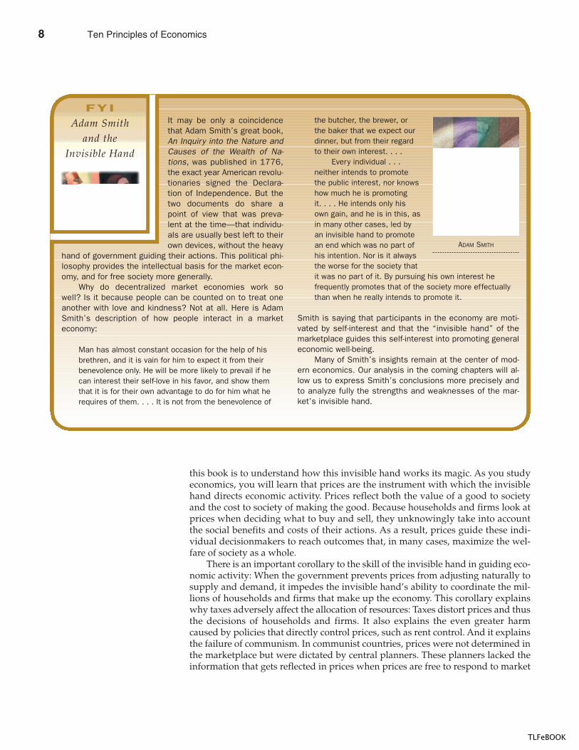
It may be only a coincidencethat Adam Smith’s great book,An Inquiry into the Nature andCauses of the Wealth of Na-tions, was published in 1776,the exact year American revolu-tionaries signed the Declara-tion of Independence. But thetwo documents do share apoint of view that was preva-lent at the time—that individu-als are usually best left to theirown devices, without the heavy
hand of government guiding their actions. This political phi-losophy provides the intellectual basis for the market econ-omy, and for free society more generally.
Why do decentralized market economies work sowell? Is it because people can be counted on to treat oneanother with love and kindness? Not at all. Here is AdamSmith’s description of how people interact in a marketeconomy:
Man has almost constant occasion for the help of hisbrethren, and it is vain for him to expect it from theirbenevolence only. He will be more likely to prevail if hecan interest their self-love in his favor, and show themthat it is for their own advantage to do for him what herequires of them. . . . It is not from the benevolence of
the butcher, the brewer, or the baker that we expect ourdinner, but from their regardto their own interest. . . .
Every individual . . .neither intends to promotethe public interest, nor knowshow much he is promotingit. . . . He intends only hisown gain, and he is in this, asin many other cases, led byan invisible hand to promotean end which was no part ofhis intention. Nor is it alwaysthe worse for the society thatit was no part of it. By pursuing his own interest hefrequently promotes that of the society more effectuallythan when he really intends to promote it.
Smith is saying that participants in the economy are moti-vated by self-interest and that the “invisible hand” of themarketplace guides this self-interest into promoting generaleconomic well-being.
Many of Smith’s insights remain at the center of mod-ern economics. Our analysis in the coming chapters will al-low us to express Smith’s conclusions more precisely andto analyze fully the strengths and weaknesses of the mar-ket’s invisible hand.
ADAM SMITH
FYI
Adam Smithand the
Invisible Hand
8 Ten Principles of Economics
TLFeBOOK
CHAPTER 1 TEN PRINCIPLES OF ECONOMICS 11
forces. Central planners failed because they tried to run the economy with onehand tied behind their backs—the invisible hand of the marketplace.
PRINCIPLE #7: GOVERNMENTS CAN SOMETIMESIMPROVE MARKET OUTCOMES
Although markets are usually a good way to organize economic activity, this rulehas some important exceptions. There are two broad reasons for a government tointervene in the economy: to promote efficiency and to promote equity. That is,most policies aim either to enlarge the economic pie or to change how the pie isdivided.
The invisible hand usually leads markets to allocate resources efficiently.Nonetheless, for various reasons, the invisible hand sometimes does not work.Economists use the term market failure to refer to a situation in which the marketon its own fails to allocate resources efficiently.
One possible cause of market failure is an externality. An externality is the im-pact of one person’s actions on the well-being of a bystander. The classic exampleof an external cost is pollution. If a chemical factory does not bear the entire cost ofthe smoke it emits, it will likely emit too much. Here, the government can raiseeconomic well-being through environmental regulation. The classic example of anexternal benefit is the creation of knowledge. When a scientist makes an importantdiscovery, he produces a valuable resource that other people can use. In this case,the government can raise economic well-being by subsidizing basic research, as infact it does.
Another possible cause of market failure is market power. Market powerrefers to the ability of a single person (or small group of people) to unduly influ-ence market prices. For example, suppose that everyone in town needs water butthere is only one well. The owner of the well has market power—in this case amonopoly—over the sale of water. The well owner is not subject to the rigorouscompetition with which the invisible hand normally keeps self-interest in check.You will learn that, in this case, regulating the price that the monopolist chargescan potentially enhance economic efficiency.
The invisible hand is even less able to ensure that economic prosperity is dis-tributed fairly. A market economy rewards people according to their ability to pro-duce things that other people are willing to pay for. The world’s best basketballplayer earns more than the world’s best chess player simply because people arewilling to pay more to watch basketball than chess. The invisible hand does not en-sure that everyone has sufficient food, decent clothing, and adequate health care.A goal of many public policies, such as the income tax and the welfare system, isto achieve a more equitable distribution of economic well-being.
To say that the government can improve on markets outcomes at times doesnot mean that it always will. Public policy is made not by angels but by a politicalprocess that is far from perfect. Sometimes policies are designed simply to rewardthe politically powerful. Sometimes they are made by well-intentioned leaderswho are not fully informed. One goal of the study of economics is to help youjudge when a government policy is justifiable to promote efficiency or equity andwhen it is not.
QUICK QUIZ: List and briefly explain the three principles concerning economic interactions.
market fa i lu rea situation in which a market left onits own fails to allocate resourcesefficiently
externa l i tythe impact of one person’s actions onthe well-being of a bystander
market powerthe ability of a single economic actor(or small group of actors) to have asubstantial influence on marketprices
Ten Principles of Economics 9
TLFeBOOK
12 PART ONE INTRODUCTION
HOW THE ECONOMY AS A WHOLE WORKS
We started by discussing how individuals make decisions and then looked at howpeople interact with one another. All these decisions and interactions togethermake up “the economy.” The last three principles concern the workings of theeconomy as a whole.
PRINCIPLE #8: A COUNTRY’S STANDARD OFLIVING DEPENDS ON ITS ABIL ITY TOPRODUCE GOODS AND SERVICES
The differences in living standards around the world are staggering. In 1997 theaverage American had an income of about $29,000. In the same year, the averageMexican earned $8,000, and the average Nigerian earned $900. Not surprisingly,this large variation in average income is reflected in various measures of the qual-ity of life. Citizens of high-income countries have more TV sets, more cars, betternutrition, better health care, and longer life expectancy than citizens of low-incomecountries.
Changes in living standards over time are also large. In the United States,incomes have historically grown about 2 percent per year (after adjusting forchanges in the cost of living). At this rate, average income doubles every 35 years.Over the past century, average income has risen about eightfold.
What explains these large differences in living standards among countries andover time? The answer is surprisingly simple. Almost all variation in living stan-dards is attributable to differences in countries’ productivity—that is, the amountof goods and services produced from each hour of a worker’s time. In nationswhere workers can produce a large quantity of goods and services per unit of time,most people enjoy a high standard of living; in nations where workers are lessproductive, most people must endure a more meager existence. Similarly, thegrowth rate of a nation’s productivity determines the growth rate of its averageincome.
The fundamental relationship between productivity and living standards issimple, but its implications are far-reaching. If productivity is the primary deter-minant of living standards, other explanations must be of secondary importance.For example, it might be tempting to credit labor unions or minimum-wage lawsfor the rise in living standards of American workers over the past century. Yet thereal hero of American workers is their rising productivity. As another example,some commentators have claimed that increased competition from Japan andother countries explains the slow growth in U.S. incomes over the past 30 years.Yet the real villain is not competition from abroad but flagging productivitygrowth in the United States.
The relationship between productivity and living standards also has profoundimplications for public policy. When thinking about how any policy will affect liv-ing standards, the key question is how it will affect our ability to produce goodsand services. To boost living standards, policymakers need to raise productivity byensuring that workers are well educated, have the tools needed to produce goodsand services, and have access to the best available technology.
product iv i tythe amount of goods and servicesproduced from each hour of aworker’s time
10 Ten Principles of Economics
TLFeBOOK
CHAPTER 1 TEN PRINCIPLES OF ECONOMICS 13
In the 1980s and 1990s, for example, much debate in the United States centeredon the government’s budget deficit—the excess of government spending over gov-ernment revenue. As we will see, concern over the budget deficit was basedlargely on its adverse impact on productivity. When the government needs tofinance a budget deficit, it does so by borrowing in financial markets, much as astudent might borrow to finance a college education or a firm might borrow tofinance a new factory. As the government borrows to finance its deficit, therefore,it reduces the quantity of funds available for other borrowers. The budget deficitthereby reduces investment both in human capital (the student’s education) andphysical capital (the firm’s factory). Because lower investment today means lowerproductivity in the future, government budget deficits are generally thought to de-press growth in living standards.
PRINCIPLE #9: PRICES RISE WHEN THEGOVERNMENT PRINTS TOO MUCH MONEY
In Germany in January 1921, a daily newspaper cost 0.30 marks. Less than twoyears later, in November 1922, the same newspaper cost 70,000,000 marks. Allother prices in the economy rose by similar amounts. This episode is one of his-tory’s most spectacular examples of inflation, an increase in the overall level ofprices in the economy.
Although the United States has never experienced inflation even close to thatin Germany in the 1920s, inflation has at times been an economic problem. Duringthe 1970s, for instance, the overall level of prices more than doubled, and PresidentGerald Ford called inflation “public enemy number one.” By contrast, inflation inthe 1990s was about 3 percent per year; at this rate it would take more than
in f lat ionan increase in the overall level ofprices in the economy
“Well it may have been 68 cents when you got in line, but it’s 74 cents now!”
Ten Principles of Economics 11
TLFeBOOK
14 PART ONE INTRODUCTION
20 years for prices to double. Because high inflation imposes various costs on soci-ety, keeping inflation at a low level is a goal of economic policymakers around theworld.
What causes inflation? In almost all cases of large or persistent inflation, theculprit turns out to be the same—growth in the quantity of money. When a gov-ernment creates large quantities of the nation’s money, the value of the moneyfalls. In Germany in the early 1920s, when prices were on average tripling everymonth, the quantity of money was also tripling every month. Although less dra-matic, the economic history of the United States points to a similar conclusion: Thehigh inflation of the 1970s was associated with rapid growth in the quantity ofmoney, and the low inflation of the 1990s was associated with slow growth in thequantity of money.
PRINCIPLE #10: SOCIETY FACES A SHORT-RUN TRADEOFFBETWEEN INFLATION AND UNEMPLOYMENT
If inflation is so easy to explain, why do policymakers sometimes have trouble rid-ding the economy of it? One reason is that reducing inflation is often thought tocause a temporary rise in unemployment. The curve that illustrates this tradeoffbetween inflation and unemployment is called the Phillips curve, after the econo-mist who first examined this relationship.
The Phillips curve remains a controversial topic among economists, but mosteconomists today accept the idea that there is a short-run tradeoff between infla-tion and unemployment. This simply means that, over a period of a year or two,many economic policies push inflation and unemployment in opposite directions.Policymakers face this tradeoff regardless of whether inflation and unemploymentboth start out at high levels (as they were in the early 1980s), at low levels (as theywere in the late 1990s), or someplace in between.
Why do we face this short-run tradeoff? According to a common explanation,it arises because some prices are slow to adjust. Suppose, for example, that thegovernment reduces the quantity of money in the economy. In the long run, theonly result of this policy change will be a fall in the overall level of prices. Yet notall prices will adjust immediately. It may take several years before all firms issuenew catalogs, all unions make wage concessions, and all restaurants print newmenus. That is, prices are said to be sticky in the short run.
Because prices are sticky, various types of government policy have short-runeffects that differ from their long-run effects. When the government reduces thequantity of money, for instance, it reduces the amount that people spend. Lowerspending, together with prices that are stuck too high, reduces the quantity ofgoods and services that firms sell. Lower sales, in turn, cause firms to lay off work-ers. Thus, the reduction in the quantity of money raises unemployment temporar-ily until prices have fully adjusted to the change.
The tradeoff between inflation and unemployment is only temporary, but itcan last for several years. The Phillips curve is, therefore, crucial for understand-ing many developments in the economy. In particular, policymakers can exploitthis tradeoff using various policy instruments. By changing the amount that thegovernment spends, the amount it taxes, and the amount of money it prints,policymakers can, in the short run, influence the combination of inflation andunemployment that the economy experiences. Because these instruments of
Phi l l ips cur vea curve that shows the short-runtradeoff between inflation andunemployment
12 Ten Principles of Economics
TLFeBOOK
CHAPTER 1 TEN PRINCIPLES OF ECONOMICS 15
monetary and fiscal policy are potentially so powerful, how policymakers shoulduse these instruments to control the economy, if at all, is a subject of continuingdebate.
QUICK QUIZ: List and briefly explain the three principles that describe how the economy as a whole works.
CONCLUSION
You now have a taste of what economics is all about. In the coming chapters wewill develop many specific insights about people, markets, and economies. Mas-tering these insights will take some effort, but it is not an overwhelming task. Thefield of economics is based on a few basic ideas that can be applied in many dif-ferent situations.
Throughout this book we will refer back to the Ten Principles of Economicshighlighted in this chapter and summarized in Table 1-1. Whenever we do so,a building-blocks icon will be displayed in the margin, as it is now. But evenwhen that icon is absent, you should keep these building blocks in mind. Even themost sophisticated economic analysis is built using the ten principles introducedhere.
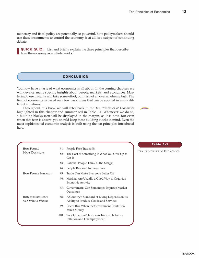
Table 1 -1
TEN PRINCIPLES OF ECONOMICSHOW PEOPLE #1: People Face TradeoffsMAKE DECISIONS #2: The Cost of Something Is What You Give Up to
Get It
#3: Rational People Think at the Margin
#4: People Respond to Incentives
HOW PEOPLE INTERACT #5: Trade Can Make Everyone Better Off
#6: Markets Are Usually a Good Way to OrganizeEconomic Activity
#7: Governments Can Sometimes Improve MarketOutcomes
HOW THE ECONOMY #8: A Country’s Standard of Living Depends on ItsAS A WHOLE WORKS Ability to Produce Goods and Services
#9: Prices Rise When the Government Prints TooMuch Money
#10: Society Faces a Short-Run Tradeoff betweenInflation and Unemployment
Ten Principles of Economics 13
TLFeBOOK
16 PART ONE INTRODUCTION
� The fundamental lessons about individualdecisionmaking are that people face tradeoffs amongalternative goals, that the cost of any action is measuredin terms of forgone opportunities, that rational peoplemake decisions by comparing marginal costs andmarginal benefits, and that people change their behaviorin response to the incentives they face.
� The fundamental lessons about interactions amongpeople are that trade can be mutually beneficial, that
markets are usually a good way of coordinating tradeamong people, and that the government can potentiallyimprove market outcomes if there is some marketfailure or if the market outcome is inequitable.
� The fundamental lessons about the economy as a wholeare that productivity is the ultimate source of livingstandards, that money growth is the ultimate source ofinflation, and that society faces a short-run tradeoffbetween inflation and unemployment.
Summar y
scarcity, p. 4economics, p. 4efficiency, p. 5equity, p. 5opportunity cost, p. 6
marginal changes, p. 6market economy, p. 9market failure, p. 11externality, p. 11market power, p. 11
productivity, p. 12inflation, p. 13Phillips curve, p. 14
Key Concepts
1. Give three examples of important tradeoffs that you facein your life.
2. What is the opportunity cost of seeing a movie?
3. Water is necessary for life. Is the marginal benefit of aglass of water large or small?
4. Why should policymakers think about incentives?
5. Why isn’t trade among countries like a game with somewinners and some losers?
6. What does the “invisible hand” of the marketplace do?
7. Explain the two main causes of market failure and givean example of each.
8. Why is productivity important?
9. What is inflation, and what causes it?
10. How are inflation and unemployment related in theshort run?
Quest ions fo r Rev iew
1. Describe some of the tradeoffs faced by the following:a. a family deciding whether to buy a new carb. a member of Congress deciding how much to
spend on national parksc. a company president deciding whether to open a
new factoryd. a professor deciding how much to prepare for class
2. You are trying to decide whether to take a vacation.Most of the costs of the vacation (airfare, hotel, forgonewages) are measured in dollars, but the benefits of thevacation are psychological. How can you compare thebenefits to the costs?
3. You were planning to spend Saturday working at yourpart-time job, but a friend asks you to go skiing. What
is the true cost of going skiing? Now suppose that youhad been planning to spend the day studying at thelibrary. What is the cost of going skiing in this case?Explain.
4. You win $100 in a basketball pool. You have a choicebetween spending the money now or putting it awayfor a year in a bank account that pays 5 percent interest.What is the opportunity cost of spending the $100 now?
5. The company that you manage has invested $5 millionin developing a new product, but the development isnot quite finished. At a recent meeting, your salespeoplereport that the introduction of competing products hasreduced the expected sales of your new product to$3 million. If it would cost $1 million to finish
Prob lems and App l icat ions
14 Ten Principles of Economics
TLFeBOOK
CHAPTER 1 TEN PRINCIPLES OF ECONOMICS 17
development and make the product, should you goahead and do so? What is the most that you should payto complete development?
6. Three managers of the Magic Potion Company arediscussing a possible increase in production. Eachsuggests a way to make this decision.
HARRY: We should examine whether ourcompany’s productivity—gallons ofpotion per worker—would rise or fall.
RON: We should examine whether our averagecost—cost per worker—would rise or fall.
HERMIONE: We should examine whether the extrarevenue from selling the additional potionwould be greater or smaller than the extracosts.
Who do you think is right? Why?
7. The Social Security system provides income for peopleover age 65. If a recipient of Social Security decides towork and earn some income, the amount he or shereceives in Social Security benefits is typically reduced.a. How does the provision of Social Security affect
people’s incentive to save while working?b. How does the reduction in benefits associated with
higher earnings affect people’s incentive to workpast age 65?
8. A recent bill reforming the government’s antipovertyprograms limited many welfare recipients to only twoyears of benefits.a. How does this change affect the incentives for
working?b. How might this change represent a tradeoff
between equity and efficiency?
9. Your roommate is a better cook than you are, but youcan clean more quickly than your roommate can. If yourroommate did all of the cooking and you did all of thecleaning, would your chores take you more or less timethan if you divided each task evenly? Give a similarexample of how specialization and trade can make twocountries both better off.
10. Suppose the United States adopted central planning forits economy, and you became the chief planner. Amongthe millions of decisions that you need to make for nextyear are how many compact discs to produce, whatartists to record, and who should receive the discs.a. To make these decisions intelligently, what
information would you need about the compactdisc industry? What information would you needabout each of the people in the United States?
b. How would your decisions about CDs affect someof your other decisions, such as how many CDplayers to make or cassette tapes to produce? Howmight some of your other decisions about theeconomy change your views about CDs?
11. Explain whether each of the following governmentactivities is motivated by a concern about equity or aconcern about efficiency. In the case of efficiency, discussthe type of market failure involved.a. regulating cable-TV pricesb. providing some poor people with vouchers that can
be used to buy foodc. prohibiting smoking in public placesd. breaking up Standard Oil (which once owned
90 percent of all oil refineries) into several smallercompanies
e. imposing higher personal income tax rates onpeople with higher incomes
f. instituting laws against driving while intoxicated
12. Discuss each of the following statements from thestandpoints of equity and efficiency.a. “Everyone in society should be guaranteed the best
health care possible.”b. “When workers are laid off, they should be able to
collect unemployment benefits until they find anew job.”
13. In what ways is your standard of living different fromthat of your parents or grandparents when they wereyour age? Why have these changes occurred?
14. Suppose Americans decide to save more of theirincomes. If banks lend this extra saving to businesses,which use the funds to build new factories, how mightthis lead to faster growth in productivity? Who do yousuppose benefits from the higher productivity? Issociety getting a free lunch?
15. Suppose that when everyone wakes up tomorrow, theydiscover that the government has given them anadditional amount of money equal to the amount theyalready had. Explain what effect this doubling of themoney supply will likely have on the following:a. the total amount spent on goods and servicesb. the quantity of goods and services purchased if
prices are stickyc. the prices of goods and services if prices can adjust
16. Imagine that you are a policymaker trying to decidewhether to reduce the rate of inflation. To make anintelligent decision, what would you need to knowabout inflation, unemployment, and the tradeoffbetween them?
Ten Principles of Economics 15
TLFeBOOK

TLFeBOOK
IN THIS CHAPTERYOU WILL . . .
Learn the di f ferencebetween posit ive andnormative statements
Learn two s implemodels—the c i r cu lar
f low and theproduct ion
poss ib i l i t ies f r ont ie r
See how economistsapp ly the methods
of sc ience
Cons ider howassumpt ions andmodels can shed
l ight on the wor ld
Dist ingu ish betweenmicroeconomics and
macroeconomics
Every field of study has its own language and its own way of thinking. Mathe-maticians talk about axioms, integrals, and vector spaces. Psychologists talk aboutego, id, and cognitive dissonance. Lawyers talk about venue, torts, and promissoryestoppel.
Economics is no different. Supply, demand, elasticity, comparative advantage,consumer surplus, deadweight loss—these terms are part of the economist’s lan-guage. In the coming chapters, you will encounter many new terms and some fa-miliar words that economists use in specialized ways. At first, this new languagemay seem needlessly arcane. But, as you will see, its value lies in its ability to pro-vide you a new and useful way of thinking about the world in which you live.
The single most important purpose of this book is to help you learn the econ-omist’s way of thinking. Of course, just as you cannot become a mathematician,psychologist, or lawyer overnight, learning to think like an economist will take
T H I N K I N G L I K E
A N E C O N O M I S T
19
Examine the ro le o feconomists inmaking po l icy
Cons ider whyeconomists
somet imes d isagreewith one another
17
2
TLFeBOOK
20 PART ONE INTRODUCTION
some time. Yet with a combination of theory, case studies, and examples of eco-nomics in the news, this book will give you ample opportunity to develop andpractice this skill.
Before delving into the substance and details of economics, it is helpful to havean overview of how economists approach the world. This chapter, therefore, dis-cusses the field’s methodology. What is distinctive about how economists confronta question? What does it mean to think like an economist?
THE ECONOMIST AS SCIENTIST
Economists try to address their subject with a scientist’s objectivity. They approachthe study of the economy in much the same way as a physicist approaches thestudy of matter and a biologist approaches the study of life: They devise theories,collect data, and then analyze these data in an attempt to verify or refute theirtheories.
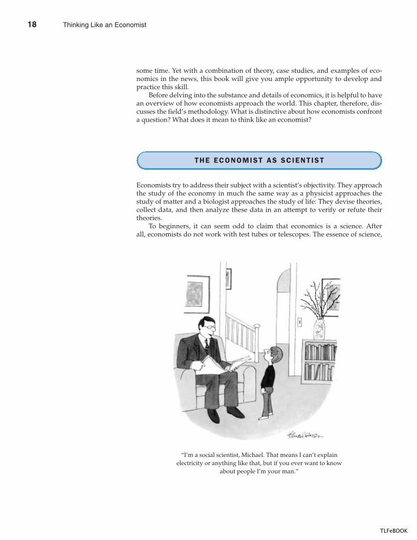
To beginners, it can seem odd to claim that economics is a science. Afterall, economists do not work with test tubes or telescopes. The essence of science,
“I’m a social scientist, Michael. That means I can’t explainelectricity or anything like that, but if you ever want to know
about people I’m your man.”
18 Thinking Like an Economist
TLFeBOOK
CHAPTER 2 THINKING L IKE AN ECONOMIST 21
however, is the scientific method—the dispassionate development and testing oftheories about how the world works. This method of inquiry is as applicable tostudying a nation’s economy as it is to studying the earth’s gravity or a species’evolution. As Albert Einstein once put it, “The whole of science is nothing morethan the refinement of everyday thinking.”
Although Einstein’s comment is as true for social sciences such as economicsas it is for natural sciences such as physics, most people are not accustomed tolooking at society through the eyes of a scientist. Let’s therefore discuss some ofthe ways in which economists apply the logic of science to examine how an econ-omy works.
THE SCIENTIF IC METHOD: OBSERVATION,THEORY, AND MORE OBSERVATION
Isaac Newton, the famous seventeenth-century scientist and mathematician, al-legedly became intrigued one day when he saw an apple fall from an apple tree.This observation motivated Newton to develop a theory of gravity that applies notonly to an apple falling to the earth but to any two objects in the universe. Subse-quent testing of Newton’s theory has shown that it works well in many circum-stances (although, as Einstein would later emphasize, not in all circumstances).Because Newton’s theory has been so successful at explaining observation, it isstill taught today in undergraduate physics courses around the world.
This interplay between theory and observation also occurs in the field of eco-nomics. An economist might live in a country experiencing rapid increases inprices and be moved by this observation to develop a theory of inflation. Thetheory might assert that high inflation arises when the government prints toomuch money. (As you may recall, this was one of the Ten Principles of Economics inChapter 1.) To test this theory, the economist could collect and analyze data onprices and money from many different countries. If growth in the quantity ofmoney were not at all related to the rate at which prices are rising, the economistwould start to doubt the validity of his theory of inflation. If money growth and in-flation were strongly correlated in international data, as in fact they are, the econ-omist would become more confident in his theory.
Although economists use theory and observation like other scientists, they doface an obstacle that makes their task especially challenging: Experiments are oftendifficult in economics. Physicists studying gravity can drop many objects in theirlaboratories to generate data to test their theories. By contrast, economists study-ing inflation are not allowed to manipulate a nation’s monetary policy simply togenerate useful data. Economists, like astronomers and evolutionary biologists,usually have to make do with whatever data the world happens to give them.
To find a substitute for laboratory experiments, economists pay close attentionto the natural experiments offered by history. When a war in the Middle East in-terrupts the flow of crude oil, for instance, oil prices skyrocket around the world.For consumers of oil and oil products, such an event depresses living standards.For economic policymakers, it poses a difficult choice about how best to respond.But for economic scientists, it provides an opportunity to study the effects of a keynatural resource on the world’s economies, and this opportunity persists long afterthe wartime increase in oil prices is over. Throughout this book, therefore, we con-sider many historical episodes. These episodes are valuable to study because they
Thinking Like an Economist 19
TLFeBOOK
22 PART ONE INTRODUCTION
give us insight into the economy of the past and, more important, because they al-low us to illustrate and evaluate economic theories of the present.
THE ROLE OF ASSUMPTIONS
If you ask a physicist how long it would take for a marble to fall from the top of aten-story building, she will answer the question by assuming that the marble fallsin a vacuum. Of course, this assumption is false. In fact, the building is surroundedby air, which exerts friction on the falling marble and slows it down. Yet the physi-cist will correctly point out that friction on the marble is so small that its effect isnegligible. Assuming the marble falls in a vacuum greatly simplifies the problemwithout substantially affecting the answer.
Economists make assumptions for the same reason: Assumptions can makethe world easier to understand. To study the effects of international trade, for ex-ample, we may assume that the world consists of only two countries and that eachcountry produces only two goods. Of course, the real world consists of dozens ofcountries, each of which produces thousands of different types of goods. But by as-suming two countries and two goods, we can focus our thinking. Once we under-stand international trade in an imaginary world with two countries and twogoods, we are in a better position to understand international trade in the morecomplex world in which we live.
The art in scientific thinking—whether in physics, biology, or economics—isdeciding which assumptions to make. Suppose, for instance, that we were drop-ping a beach ball rather than a marble from the top of the building. Our physicistwould realize that the assumption of no friction is far less accurate in this case:Friction exerts a greater force on a beach ball than on a marble. The assumptionthat gravity works in a vacuum is reasonable for studying a falling marble but notfor studying a falling beach ball.
Similarly, economists use different assumptions to answer different questions.Suppose that we want to study what happens to the economy when the govern-ment changes the number of dollars in circulation. An important piece of thisanalysis, it turns out, is how prices respond. Many prices in the economy changeinfrequently; the newsstand prices of magazines, for instance, are changed onlyevery few years. Knowing this fact may lead us to make different assumptionswhen studying the effects of the policy change over different time horizons. Forstudying the short-run effects of the policy, we may assume that prices do notchange much. We may even make the extreme and artificial assumption that allprices are completely fixed. For studying the long-run effects of the policy, how-ever, we may assume that all prices are completely flexible. Just as a physicist usesdifferent assumptions when studying falling marbles and falling beach balls, econ-omists use different assumptions when studying the short-run and long-run ef-fects of a change in the quantity of money.
ECONOMIC MODELS
High school biology teachers teach basic anatomy with plastic replicas of the hu-man body. These models have all the major organs—the heart, the liver, the kid-neys, and so on. The models allow teachers to show their students in a simple wayhow the important parts of the body fit together. Of course, these plastic models
20 Thinking Like an Economist
TLFeBOOK
CHAPTER 2 THINKING L IKE AN ECONOMIST 23
are not actual human bodies, and no one would mistake the model for a real per-son. These models are stylized, and they omit many details. Yet despite this lack ofrealism—indeed, because of this lack of realism—studying these models is usefulfor learning how the human body works.
Economists also use models to learn about the world, but instead of beingmade of plastic, they are most often composed of diagrams and equations. Likea biology teacher’s plastic model, economic models omit many details to allowus to see what is truly important. Just as the biology teacher’s model does not in-clude all of the body’s muscles and capillaries, an economist’s model does notinclude every feature of the economy.
As we use models to examine various economic issues throughout this book,you will see that all the models are built with assumptions. Just as a physicist be-gins the analysis of a falling marble by assuming away the existence of friction,economists assume away many of the details of the economy that are irrelevant forstudying the question at hand. All models—in physics, biology, or economics—simplify reality in order to improve our understanding of it.
OUR FIRST MODEL: THE CIRCULAR-FLOW DIAGRAM
The economy consists of millions of people engaged in many activities—buying,selling, working, hiring, manufacturing, and so on. To understand how the econ-omy works, we must find some way to simplify our thinking about all these activ-ities. In other words, we need a model that explains, in general terms, how theeconomy is organized and how participants in the economy interact with oneanother.
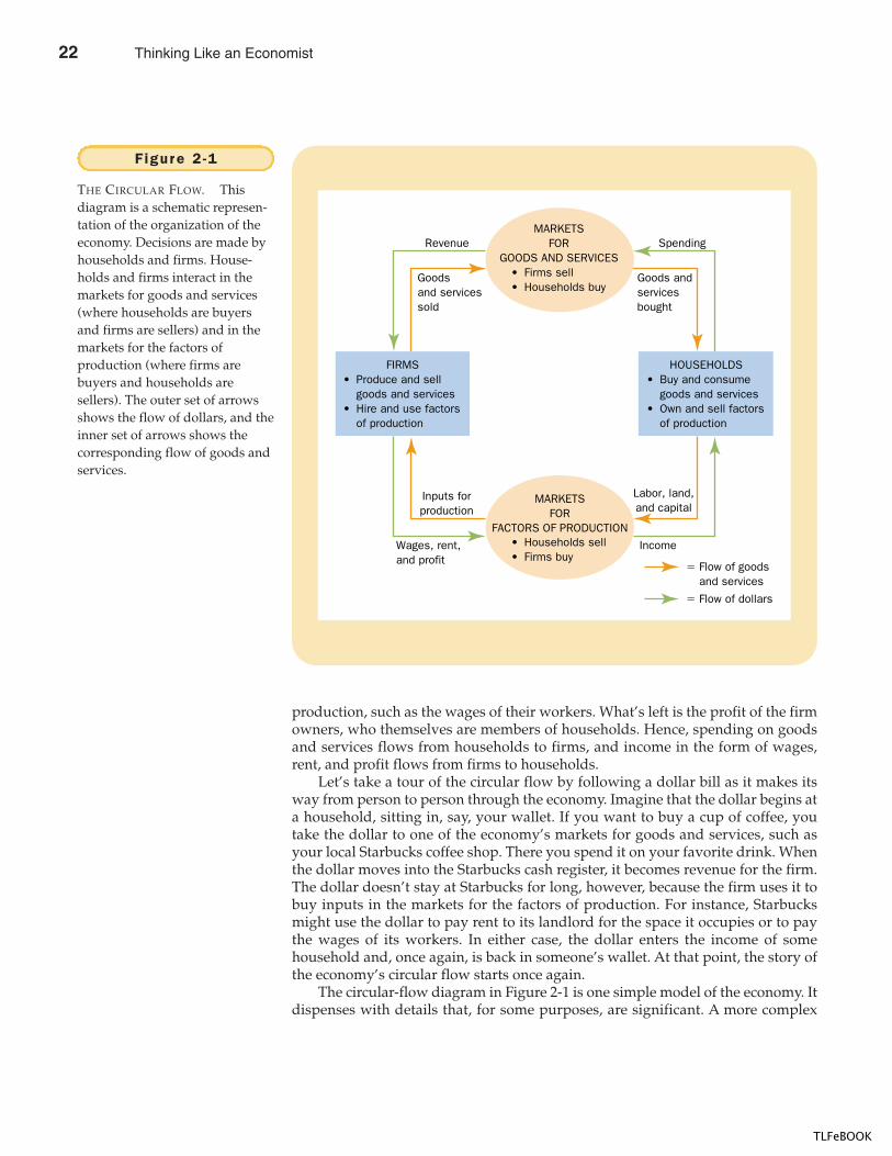
Figure 2-1 presents a visual model of the economy, called a circular-flowdiagram. In this model, the economy has two types of decisionmakers—house-holds and firms. Firms produce goods and services using inputs, such as labor,land, and capital (buildings and machines). These inputs are called the factors ofproduction. Households own the factors of production and consume all the goodsand services that the firms produce.
Households and firms interact in two types of markets. In the markets forgoods and services, households are buyers and firms are sellers. In particular,households buy the output of goods and services that firms produce. In the mar-kets for the factors of production, households are sellers and firms are buyers. Inthese markets, households provide firms the inputs that the firms use to producegoods and services. The circular-flow diagram offers a simple way of organizingall the economic transactions that occur between households and firms in theeconomy.
The inner loop of the circular-flow diagram represents the flows of goods andservices between households and firms. The households sell the use of their labor,land, and capital to the firms in the markets for the factors of production. The firmsthen use these factors to produce goods and services, which in turn are soldto households in the markets for goods and services. Hence, the factors of produc-tion flow from households to firms, and goods and services flow from firms tohouseholds.
The outer loop of the circular-flow diagram represents the corresponding flowof dollars. The households spend money to buy goods and services from thefirms. The firms use some of the revenue from these sales to pay for the factors of
c i rcu la r - f low d iagrama visual model of the economy thatshows how dollars flow throughmarkets among households and firms
Thinking Like an Economist 21
TLFeBOOK
24 PART ONE INTRODUCTION
production, such as the wages of their workers. What’s left is the profit of the firmowners, who themselves are members of households. Hence, spending on goodsand services flows from households to firms, and income in the form of wages,rent, and profit flows from firms to households.
Let’s take a tour of the circular flow by following a dollar bill as it makes itsway from person to person through the economy. Imagine that the dollar begins ata household, sitting in, say, your wallet. If you want to buy a cup of coffee, youtake the dollar to one of the economy’s markets for goods and services, such asyour local Starbucks coffee shop. There you spend it on your favorite drink. Whenthe dollar moves into the Starbucks cash register, it becomes revenue for the firm.The dollar doesn’t stay at Starbucks for long, however, because the firm uses it tobuy inputs in the markets for the factors of production. For instance, Starbucksmight use the dollar to pay rent to its landlord for the space it occupies or to paythe wages of its workers. In either case, the dollar enters the income of somehousehold and, once again, is back in someone’s wallet. At that point, the story ofthe economy’s circular flow starts once again.
The circular-flow diagram in Figure 2-1 is one simple model of the economy. Itdispenses with details that, for some purposes, are significant. A more complex
Spending
Goods andservicesbought
Revenue
Goodsand servicessold
Labor, land,and capital
Income
� Flow of goodsand services
� Flow of dollars
Inputs forproduction
Wages, rent,and profit
FIRMS• Produce and sell
goods and services• Hire and use factors
of production
• Buy and consumegoods and services
• Own and sell factorsof production
HOUSEHOLDS
• Households sell• Firms buy
MARKETSFOR
FACTORS OF PRODUCTION
• Firms sell• Households buy
MARKETSFOR
GOODS AND SERVICES
Figure 2 -1
THE CIRCULAR FLOW. Thisdiagram is a schematic represen-tation of the organization of theeconomy. Decisions are made byhouseholds and firms. House-holds and firms interact in themarkets for goods and services(where households are buyersand firms are sellers) and in themarkets for the factors ofproduction (where firms arebuyers and households aresellers). The outer set of arrowsshows the flow of dollars, and theinner set of arrows shows thecorresponding flow of goods andservices.
22 Thinking Like an Economist
TLFeBOOK
CHAPTER 2 THINKING L IKE AN ECONOMIST 25
and realistic circular-flow model would include, for instance, the roles of govern-ment and international trade. Yet these details are not crucial for a basic under-standing of how the economy is organized. Because of its simplicity, thiscircular-flow diagram is useful to keep in mind when thinking about how thepieces of the economy fit together.
OUR SECOND MODEL: THE PRODUCTIONPOSSIBIL IT IES FRONTIER
Most economic models, unlike the circular-flow diagram, are built using the toolsof mathematics. Here we consider one of the simplest such models, called the pro-duction possibilities frontier, and see how this model illustrates some basic eco-nomic ideas.
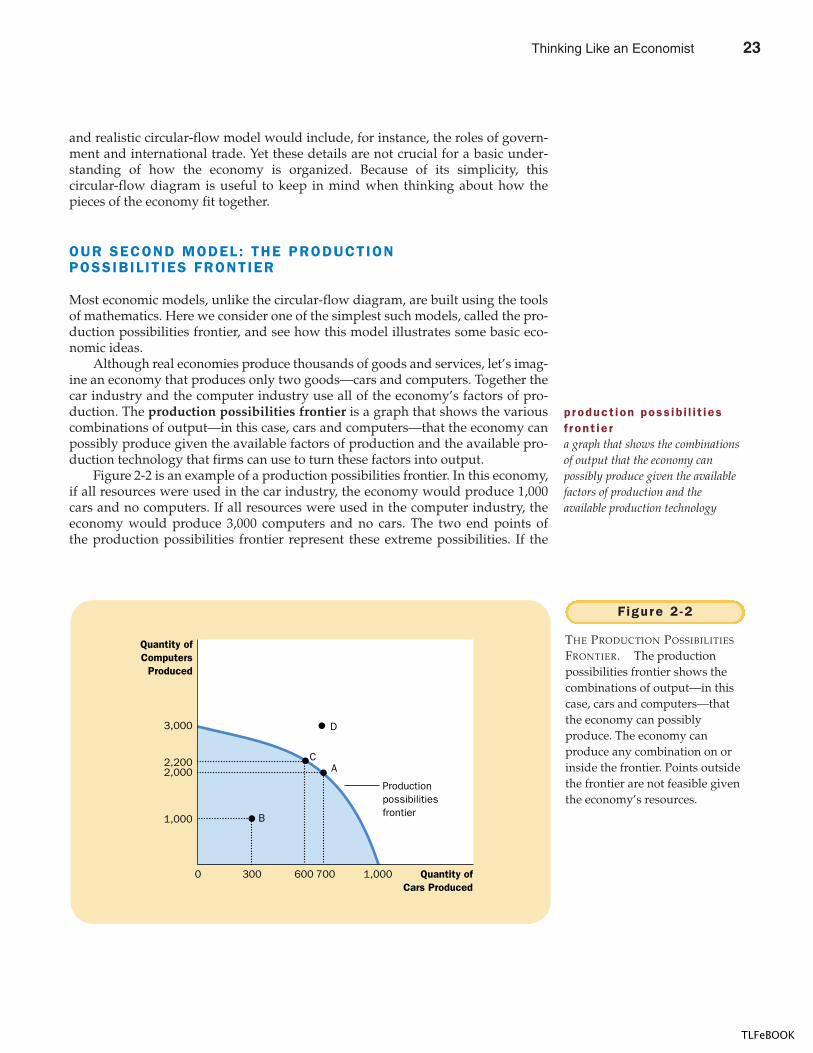
Although real economies produce thousands of goods and services, let’s imag-ine an economy that produces only two goods—cars and computers. Together thecar industry and the computer industry use all of the economy’s factors of pro-duction. The production possibilities frontier is a graph that shows the variouscombinations of output—in this case, cars and computers—that the economy canpossibly produce given the available factors of production and the available pro-duction technology that firms can use to turn these factors into output.
Figure 2-2 is an example of a production possibilities frontier. In this economy,if all resources were used in the car industry, the economy would produce 1,000cars and no computers. If all resources were used in the computer industry, theeconomy would produce 3,000 computers and no cars. The two end points ofthe production possibilities frontier represent these extreme possibilities. If the
1,000
2,200
Productionpossibilitiesfrontier
A
B
C
Quantity ofCars Produced
7006003000
2,000
3,000
1,000
Quantity ofComputers
Produced
D
Figure 2 -2
THE PRODUCTION POSSIBILITIES
FRONTIER. The productionpossibilities frontier shows thecombinations of output—in thiscase, cars and computers—thatthe economy can possiblyproduce. The economy canproduce any combination on orinside the frontier. Points outsidethe frontier are not feasible giventhe economy’s resources.
product ion poss ib i l i t iesf ront ie ra graph that shows the combinationsof output that the economy canpossibly produce given the availablefactors of production and theavailable production technology
Thinking Like an Economist 23
TLFeBOOK
26 PART ONE INTRODUCTION
economy were to divide its resources between the two industries, it could produce700 cars and 2,000 computers, shown in the figure by point A. By contrast, the out-come at point D is not possible because resources are scarce: The economy doesnot have enough of the factors of production to support that level of output. Inother words, the economy can produce at any point on or inside the productionpossibilities frontier, but it cannot produce at points outside the frontier.
An outcome is said to be efficient if the economy is getting all it can from thescarce resources it has available. Points on (rather than inside) the production pos-sibilities frontier represent efficient levels of production. When the economy is pro-ducing at such a point, say point A, there is no way to produce more of one goodwithout producing less of the other. Point B represents an inefficient outcome. Forsome reason, perhaps widespread unemployment, the economy is producing lessthan it could from the resources it has available: It is producing only 300 cars and1,000 computers. If the source of the inefficiency were eliminated, the economycould move from point B to point A, increasing production of both cars (to 700)and computers (to 2,000).
One of the Ten Principles of Economics discussed in Chapter 1 is that people facetradeoffs. The production possibilities frontier shows one tradeoff that societyfaces. Once we have reached the efficient points on the frontier, the only way ofgetting more of one good is to get less of the other. When the economy moves frompoint A to point C, for instance, society produces more computers but at the ex-pense of producing fewer cars.
Another of the Ten Principles of Economics is that the cost of something is whatyou give up to get it. This is called the opportunity cost. The production possibilitiesfrontier shows the opportunity cost of one good as measured in terms of the othergood. When society reallocates some of the factors of production from the car in-dustry to the computer industry, moving the economy from point A to point C, itgives up 100 cars to get 200 additional computers. In other words, when the econ-omy is at point A, the opportunity cost of 200 computers is 100 cars.
Notice that the production possibilities frontier in Figure 2-2 is bowed out-ward. This means that the opportunity cost of cars in terms of computers dependson how much of each good the economy is producing. When the economy is usingmost of its resources to make cars, the production possibilities frontier is quitesteep. Because even workers and machines best suited to making computers arebeing used to make cars, the economy gets a substantial increase in the number ofcomputers for each car it gives up. By contrast, when the economy is using most ofits resources to make computers, the production possibilities frontier is quite flat.In this case, the resources best suited to making computers are already in the com-puter industry, and each car the economy gives up yields only a small increase inthe number of computers.
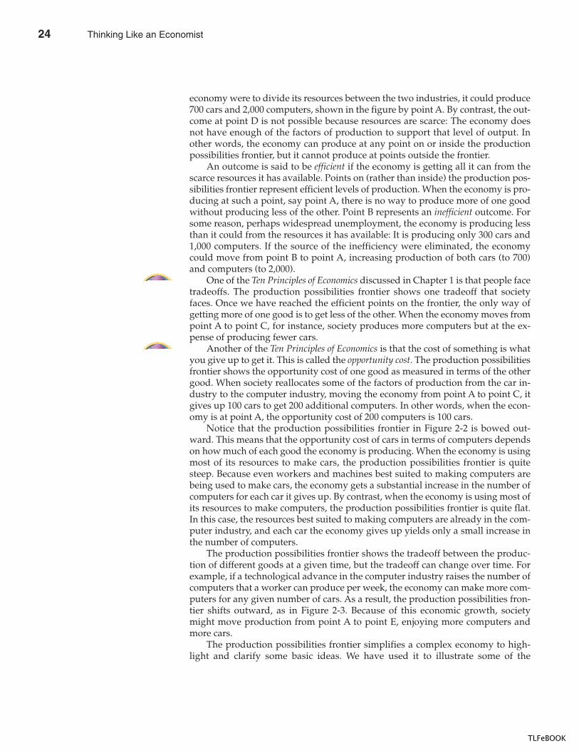
The production possibilities frontier shows the tradeoff between the produc-tion of different goods at a given time, but the tradeoff can change over time. Forexample, if a technological advance in the computer industry raises the number ofcomputers that a worker can produce per week, the economy can make more com-puters for any given number of cars. As a result, the production possibilities fron-tier shifts outward, as in Figure 2-3. Because of this economic growth, societymight move production from point A to point E, enjoying more computers andmore cars.
The production possibilities frontier simplifies a complex economy to high-light and clarify some basic ideas. We have used it to illustrate some of the
24 Thinking Like an Economist
TLFeBOOK
CHAPTER 2 THINKING L IKE AN ECONOMIST 27
concepts mentioned briefly in Chapter 1: scarcity, efficiency, tradeoffs, opportunitycost, and economic growth. As you study economics, these ideas will recur invarious forms. The production possibilities frontier offers one simple way of think-ing about them.
MICROECONOMICS AND MACROECONOMICS
Many subjects are studied on various levels. Consider biology, for example. Molec-ular biologists study the chemical compounds that make up living things. Cellularbiologists study cells, which are made up of many chemical compounds and, atthe same time, are themselves the building blocks of living organisms. Evolution-ary biologists study the many varieties of animals and plants and how specieschange gradually over the centuries.
Economics is also studied on various levels. We can study the decisions of in-dividual households and firms. Or we can study the interaction of households andfirms in markets for specific goods and services. Or we can study the operation ofthe economy as a whole, which is just the sum of the activities of all these decision-makers in all these markets.
The field of economics is traditionally divided into two broad subfields.Microeconomics is the study of how households and firms make decisions andhow they interact in specific markets. Macroeconomics is the study of economy-wide phenomena. A microeconomist might study the effects of rent control onhousing in New York City, the impact of foreign competition on the U.S. auto in-dustry, or the effects of compulsory school attendance on workers’ earnings. A
2,1002,000
A
E
Quantity ofCars Produced
700 7500
4,000
3,000
1,000
Quantity ofComputers
Produced
F igure 2 -3
A SHIFT IN THE PRODUCTION
POSSIBILITIES FRONTIER. Aneconomic advance in thecomputer industry shifts theproduction possibilities frontieroutward, increasing the numberof cars and computers theeconomy can produce.
microeconomicsthe study of how households andfirms make decisions and how theyinteract in markets
macroeconomicsthe study of economy-widephenomena, including inflation,unemployment, and economicgrowth
Thinking Like an Economist 25
TLFeBOOK
28 PART ONE INTRODUCTION
macroeconomist might study the effects of borrowing by the federal government,the changes over time in the economy’s rate of unemployment, or alternative poli-cies to raise growth in national living standards.
Microeconomics and macroeconomics are closely intertwined. Becausechanges in the overall economy arise from the decisions of millions of individuals,it is impossible to understand macroeconomic developments without consideringthe associated microeconomic decisions. For example, a macroeconomist mightstudy the effect of a cut in the federal income tax on the overall production ofgoods and services. To analyze this issue, he or she must consider how the taxcut affects the decisions of households about how much to spend on goods andservices.
Despite the inherent link between microeconomics and macroeconomics, thetwo fields are distinct. In economics, as in biology, it may seem natural to beginwith the smallest unit and build up. Yet doing so is neither necessary nor alwaysthe best way to proceed. Evolutionary biology is, in a sense, built upon molecularbiology, since species are made up of molecules. Yet molecular biology and evolu-tionary biology are separate fields, each with its own questions and its own meth-ods. Similarly, because microeconomics and macroeconomics address differentquestions, they sometimes take quite different approaches and are often taught inseparate courses.
QUICK QUIZ: In what sense is economics like a science? � Draw a production possibilities frontier for a society that produces food and clothing. Show an efficient point, an inefficient point, and an infeasible point. Show the effects of a drought. � Define microeconomics and macroeconomics.
THE ECONOMIST AS POLICY ADVISER
Often economists are asked to explain the causes of economic events. Why, for ex-ample, is unemployment higher for teenagers than for older workers? Sometimeseconomists are asked to recommend policies to improve economic outcomes.What, for instance, should the government do to improve the economic well-beingof teenagers? When economists are trying to explain the world, they are scientists.When they are trying to help improve it, they are policy advisers.
POSITIVE VERSUS NORMATIVE ANALYSIS
To help clarify the two roles that economists play, we begin by examining the useof language. Because scientists and policy advisers have different goals, they uselanguage in different ways.
For example, suppose that two people are discussing minimum-wage laws.Here are two statements you might hear:
POLLY: Minimum-wage laws cause unemployment.NORMA: The government should raise the minimum wage.
26 Thinking Like an Economist
TLFeBOOK
CHAPTER 2 THINKING L IKE AN ECONOMIST 29
Ignoring for now whether you agree with these statements, notice that Polly andNorma differ in what they are trying to do. Polly is speaking like a scientist: She ismaking a claim about how the world works. Norma is speaking like a policy ad-viser: She is making a claim about how she would like to change the world.
In general, statements about the world are of two types. One type, such asPolly’s, is positive. Positive statements are descriptive. They make a claim abouthow the world is. A second type of statement, such as Norma’s, is normative. Nor-mative statements are prescriptive. They make a claim about how the world oughtto be.
A key difference between positive and normative statements is how we judgetheir validity. We can, in principle, confirm or refute positive statements by exam-ining evidence. An economist might evaluate Polly’s statement by analyzing dataon changes in minimum wages and changes in unemployment over time. By con-trast, evaluating normative statements involves values as well as facts. Norma’sstatement cannot be judged using data alone. Deciding what is good or bad policyis not merely a matter of science. It also involves our views on ethics, religion, andpolitical philosophy.
Of course, positive and normative statements may be related. Our positiveviews about how the world works affect our normative views about what policiesare desirable. Polly’s claim that the minimum wage causes unemployment, if true,might lead us to reject Norma’s conclusion that the government should raise theminimum wage. Yet our normative conclusions cannot come from positive analy-sis alone. Instead, they require both positive analysis and value judgments.
As you study economics, keep in mind the distinction between positive andnormative statements. Much of economics just tries to explain how the economyworks. Yet often the goal of economics is to improve how the economy works.When you hear economists making normative statements, you know they havecrossed the line from scientist to policy adviser.
ECONOMISTS IN WASHINGTON
President Harry Truman once said that he wanted to find a one-armed economist.When he asked his economists for advice, they always answered, “On the onehand, . . . . On the other hand, . . . .”
Truman was right in realizing that economists’ advice is not always straight-forward. This tendency is rooted in one of the Ten Principles of Economics in Chap-ter 1: People face tradeoffs. Economists are aware that tradeoffs are involved inmost policy decisions. A policy might increase efficiency at the cost of equity. Itmight help future generations but hurt current generations. An economist whosays that all policy decisions are easy is an economist not to be trusted.
Truman was also not alone among presidents in relying on the advice of econ-omists. Since 1946, the president of the United States has received guidance fromthe Council of Economic Advisers, which consists of three members and a staff ofseveral dozen economists. The council, whose offices are just a few steps from theWhite House, has no duty other than to advise the president and to write the an-nual Economic Report of the President.
The president also receives input from economists in many administrative de-partments. Economists at the Department of Treasury help design tax policy. Econ-omists at the Department of Labor analyze data on workers and those looking for
pos i t ive statementsclaims that attempt to describe theworld as it is
normat ive statementsclaims that attempt to prescribe howthe world should be
Thinking Like an Economist 27
TLFeBOOK
30 PART ONE INTRODUCTION
work in order to help formulate labor-market policies. Economists at the Depart-ment of Justice help enforce the nation’s antitrust laws.
Economists are also found outside the administrative branch of government.To obtain independent evaluations of policy proposals, Congress relies on the ad-vice of the Congressional Budget Office, which is staffed by economists. The Fed-eral Reserve, the quasi-governmental institution that sets the nation’s monetarypolicy, employs hundreds of economists to analyze economic developments in theUnited States and throughout the world. Table 2-1 lists the Web sites of some ofthese agencies.
The influence of economists on policy goes beyond their role as advisers: Theirresearch and writings often affect policy indirectly. Economist John MaynardKeynes offered this observation:
The ideas of economists and political philosophers, both when they are right andwhen they are wrong, are more powerful than is commonly understood. Indeed,the world is ruled by little else. Practical men, who believe themselves to be quiteexempt from intellectual influences, are usually the slaves of some defuncteconomist. Madmen in authority, who hear voices in the air, are distilling theirfrenzy from some academic scribbler of a few years back.
“Let’s switch. I’ll make the policy, you implement it, and he’ll explain it.”
Table 2 -1
WEB SITES. Here are the Websites for a few of the governmentagencies that are responsible forcollecting economic data andmaking economic policy.
Department of Commerce www.doc.govBureau of Labor Statistics www.bls.govCongressional Budget Office www.cbo.govFederal Reserve Board www.federalreserve.gov
28 Thinking Like an Economist
TLFeBOOK
CHAPTER 2 THINKING L IKE AN ECONOMIST 31
Although these words were written in 1935, they remain true today. Indeed, the“academic scribbler” now influencing public policy is often Keynes himself.
QUICK QUIZ: Give an example of a positive statement and an example of a normative statement. � Name three parts of government that regularly rely on advice from economists.
WHY ECONOMISTS DISAGREE
“If all economists were laid end to end, they would not reach a conclusion.” Thisquip from George Bernard Shaw is revealing. Economists as a group are often crit-icized for giving conflicting advice to policymakers. President Ronald Reagan oncejoked that if the game Trivial Pursuit were designed for economists, it would have100 questions and 3,000 answers.
Why do economists so often appear to give conflicting advice to policy-makers? There are two basic reasons:
� Economists may disagree about the validity of alternative positive theoriesabout how the world works.
� Economists may have different values and, therefore, different normativeviews about what policy should try to accomplish.
Let’s discuss each of these reasons.
DIFFERENCES IN SCIENTIF IC JUDGMENTS
Several centuries ago, astronomers debated whether the earth or the sun was at thecenter of the solar system. More recently, meteorologists have debated whetherthe earth is experiencing “global warming” and, if so, why. Science is a search forunderstanding about the world around us. It is not surprising that as the searchcontinues, scientists can disagree about the direction in which truth lies.
Economists often disagree for the same reason. Economics is a young science,and there is still much to be learned. Economists sometimes disagree because theyhave different hunches about the validity of alternative theories or about the sizeof important parameters.
For example, economists disagree about whether the government should levytaxes based on a household’s income or its consumption (spending). Advocates ofa switch from the current income tax to a consumption tax believe that the changewould encourage households to save more, because income that is saved wouldnot be taxed. Higher saving, in turn, would lead to more rapid growth in pro-ductivity and living standards. Advocates of the current income tax believe thathousehold saving would not respond much to a change in the tax laws. Thesetwo groups of economists hold different normative views about the tax systembecause they have different positive views about the responsiveness of saving totax incentives.
Thinking Like an Economist 29
TLFeBOOK
32 PART ONE INTRODUCTION
DIFFERENCES IN VALUES
Suppose that Peter and Paul both take the same amount of water from the townwell. To pay for maintaining the well, the town taxes its residents. Peter has in-come of $50,000 and is taxed $5,000, or 10 percent of his income. Paul has incomeof $10,000 and is taxed $2,000, or 20 percent of his income.
Is this policy fair? If not, who pays too much and who pays too little? Does itmatter whether Paul’s low income is due to a medical disability or to his decisionto pursue a career in acting? Does it matter whether Peter’s high income is due toa large inheritance or to his willingness to work long hours at a dreary job?
These are difficult questions on which people are likely to disagree. If the townhired two experts to study how the town should tax its residents to pay for thewell, we would not be surprised if they offered conflicting advice.
This simple example shows why economists sometimes disagree about publicpolicy. As we learned earlier in our discussion of normative and positive analysis,policies cannot be judged on scientific grounds alone. Economists give conflictingadvice sometimes because they have different values. Perfecting the science of eco-nomics will not tell us whether it is Peter or Paul who pays too much.
PERCEPTION VERSUS REALITY
Because of differences in scientific judgments and differences in values, some disagreement among economists is inevitable. Yet one should not over-state the amount of disagreement. In many cases, economists do offer a unitedview.
Table 2-2 contains ten propositions about economic policy. In a survey ofeconomists in business, government, and academia, these propositions were en-dorsed by an overwhelming majority of respondents. Most of these propositionswould fail to command a similar consensus among the general public.
The first proposition in the table is about rent control. For reasons we will dis-cuss in Chapter 6, almost all economists believe that rent control adversely affectsthe availability and quality of housing and is a very costly way of helping the mostneedy members of society. Nonetheless, many city governments choose to ignorethe advice of economists and place ceilings on the rents that landlords may chargetheir tenants.
The second proposition in the table concerns tariffs and import quotas. Forreasons we will discuss in Chapter 3 and more fully in Chapter 9, almost all econ-omists oppose such barriers to free trade. Nonetheless, over the years, the presi-dent and Congress have chosen to restrict the import of certain goods. In 1993 theNorth American Free Trade Agreement (NAFTA), which reduced barriers to tradeamong the United States, Canada, and Mexico, passed Congress, but only by anarrow margin, despite overwhelming support from economists. In this case,economists did offer united advice, but many members of Congress chose to ig-nore it.
Why do policies such as rent control and import quotas persist if the expertsare united in their opposition? The reason may be that economists have not yetconvinced the general public that these policies are undesirable. One purpose ofthis book is to make you understand the economist’s view of these and other sub-jects and, perhaps, to persuade you that it is the right one.
30 Thinking Like an Economist
TLFeBOOK
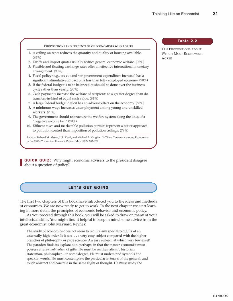
CHAPTER 2 THINKING L IKE AN ECONOMIST 33
QUICK QUIZ: Why might economic advisers to the president disagree about a question of policy?
LET’S GET GOING
The first two chapters of this book have introduced you to the ideas and methodsof economics. We are now ready to get to work. In the next chapter we start learn-ing in more detail the principles of economic behavior and economic policy.
As you proceed through this book, you will be asked to draw on many of yourintellectual skills. You might find it helpful to keep in mind some advice from thegreat economist John Maynard Keynes:
The study of economics does not seem to require any specialized gifts of anunusually high order. Is it not . . . a very easy subject compared with the higherbranches of philosophy or pure science? An easy subject, at which very few excel!The paradox finds its explanation, perhaps, in that the master-economist mustpossess a rare combination of gifts. He must be mathematician, historian,statesman, philosopher—in some degree. He must understand symbols andspeak in words. He must contemplate the particular in terms of the general, andtouch abstract and concrete in the same flight of thought. He must study the
Table 2 -2
TEN PROPOSITIONS ABOUT
WHICH MOST ECONOMISTS
AGREE
PROPOSITION (AND PERCENTAGE OF ECONOMISTS WHO AGREE)
1. A ceiling on rents reduces the quantity and quality of housing available.(93%)
2. Tariffs and import quotas usually reduce general economic welfare. (93%)3. Flexible and floating exchange rates offer an effective international monetary
arrangement. (90%)4. Fiscal policy (e.g., tax cut and/or government expenditure increase) has a
significant stimulative impact on a less than fully employed economy. (90%)5. If the federal budget is to be balanced, it should be done over the business
cycle rather than yearly. (85%)6. Cash payments increase the welfare of recipients to a greater degree than do
transfers-in-kind of equal cash value. (84%)7. A large federal budget deficit has an adverse effect on the economy. (83%)8. A minimum wage increases unemployment among young and unskilled
workers. (79%)9. The government should restructure the welfare system along the lines of a
“negative income tax.” (79%)10. Effluent taxes and marketable pollution permits represent a better approach
to pollution control than imposition of pollution ceilings. (78%)
SOURCE: Richard M. Alston, J. R. Kearl, and Michael B. Vaughn, “Is There Consensus among Economistsin the 1990s?” American Economic Review (May 1992): 203–209.
Thinking Like an Economist 31
TLFeBOOK
34 PART ONE INTRODUCTION
present in the light of the past for the purposes of the future. No part of man’snature or his institutions must lie entirely outside his regard. He must bepurposeful and disinterested in a simultaneous mood; as aloof and incorruptibleas an artist, yet sometimes as near the earth as a politician.
It is a tall order. But with practice, you will become more and more accustomed tothinking like an economist.
� Economists try to address their subject with a scientist’sobjectivity. Like all scientists, they make appropriateassumptions and build simplified models in order tounderstand the world around them. Two simpleeconomic models are the circular-flow diagram and theproduction possibilities frontier.
� The field of economics is divided into two subfields:microeconomics and macroeconomics. Microeconomistsstudy decisionmaking by households and firms and theinteraction among households and firms in themarketplace. Macroeconomists study the forces andtrends that affect the economy as a whole.
� A positive statement is an assertion about how theworld is. A normative statement is an assertion abouthow the world ought to be. When economists makenormative statements, they are acting more as policyadvisers than scientists.
� Economists who advise policymakers offer conflictingadvice either because of differences in scientificjudgments or because of differences in values. At othertimes, economists are united in the advice they offer, butpolicymakers may choose to ignore it.
Summar y
circular-flow diagram, p. 23production possibilities frontier, p. 25
microeconomics, p. 27macroeconomics, p. 27
positive statements, p. 29normative statements, p. 29
Key Concepts
1. How is economics like a science?
2. Why do economists make assumptions?
3. Should an economic model describe reality exactly?
4. Draw and explain a production possibilities frontier foran economy that produces milk and cookies. Whathappens to this frontier if disease kills half of theeconomy’s cow population?
5. Use a production possibilities frontier to describe theidea of “efficiency.”
6. What are the two subfields into which economics isdivided? Explain what each subfield studies.
7. What is the difference between a positive and anormative statement? Give an example of each.
8. What is the Council of Economic Advisers?
9. Why do economists sometimes offer conflicting adviceto policymakers?
Quest ions fo r Rev iew
32 Thinking Like an Economist
TLFeBOOK
CHAPTER 2 THINKING L IKE AN ECONOMIST 35
1. Describe some unusual language used in one of theother fields that you are studying. Why are these specialterms useful?
2. One common assumption in economics is that theproducts of different firms in the same industry areindistinguishable. For each of the following industries,discuss whether this is a reasonable assumption.a. steelb. novelsc. wheatd. fast food
3. Draw a circular-flow diagram. Identify the parts of themodel that correspond to the flow of goods and servicesand the flow of dollars for each of the followingactivities.a. Sam pays a storekeeper $1 for a quart of milk.b. Sally earns $4.50 per hour working at a fast food
restaurant.c. Serena spends $7 to see a movie.d. Stuart earns $10,000 from his 10 percent ownership
of Acme Industrial.
4. Imagine a society that produces military goods andconsumer goods, which we’ll call “guns” and “butter.”a. Draw a production possibilities frontier for guns
and butter. Explain why it most likely has a bowed-out shape.
b. Show a point that is impossible for the economy toachieve. Show a point that is feasible but inefficient.
c. Imagine that the society has two political parties,called the Hawks (who want a strong military) andthe Doves (who want a smaller military). Show apoint on your production possibilities frontier thatthe Hawks might choose and a point the Dovesmight choose.
d. Imagine that an aggressive neighboring countryreduces the size of its military. As a result, both theHawks and the Doves reduce their desiredproduction of guns by the same amount. Whichparty would get the bigger “peace dividend,”measured by the increase in butter production?Explain.
5. The first principle of economics discussed in Chapter 1is that people face tradeoffs. Use a productionpossibilities frontier to illustrate society’s tradeoffbetween a clean environment and high incomes. Whatdo you suppose determines the shape and position ofthe frontier? Show what happens to the frontier if
engineers develop an automobile engine with almost noemissions.
6. Classify the following topics as relating tomicroeconomics or macroeconomics.a. a family’s decision about how much income to saveb. the effect of government regulations on auto
emissionsc. the impact of higher national saving on economic
growthd. a firm’s decision about how many workers to hiree. the relationship between the inflation rate and
changes in the quantity of money
7. Classify each of the following statements as positive ornormative. Explain.a. Society faces a short-run tradeoff between inflation
and unemployment.b. A reduction in the rate of growth of money will
reduce the rate of inflation.c. The Federal Reserve should reduce the rate of
growth of money.d. Society ought to require welfare recipients to look
for jobs.e. Lower tax rates encourage more work and more
saving.
8. Classify each of the statements in Table 2-2 as positive,normative, or ambiguous. Explain.
9. If you were president, would you be more interested inyour economic advisers’ positive views or theirnormative views? Why?
10. The Economic Report of the President contains statisticalinformation about the economy as well as the Council ofEconomic Advisers’ analysis of current policy issues.Find a recent copy of this annual report at your libraryand read a chapter about an issue that interests you.Summarize the economic problem at hand and describethe council’s recommended policy.
11. Who is the current chairman of the Federal Reserve?Who is the current chair of the Council of EconomicAdvisers? Who is the current secretary of the treasury?
12. Look up one of the Web sites listed in Table 2-1. Whatrecent economic trends or issues are addressed there?
13. Would you expect economists to disagree less aboutpublic policy as time goes on? Why or why not? Cantheir differences be completely eliminated? Why orwhy not?
Prob lems and App l icat ions
Thinking Like an Economist 33
TLFeBOOK
A P P E N D I X
G R A P H I N G : A B R I E F R E V I E W
Many of the concepts that economists study can be expressed with numbers—theprice of bananas, the quantity of bananas sold, the cost of growing bananas, and soon. Often these economic variables are related to one another. When the price ofbananas rises, people buy fewer bananas. One way of expressing the relationshipsamong variables is with graphs.
Graphs serve two purposes. First, when developing economic theories, graphsoffer a way to visually express ideas that might be less clear if described withequations or words. Second, when analyzing economic data, graphs provide away of finding how variables are in fact related in the world. Whether we areworking with theory or with data, graphs provide a lens through which a recog-nizable forest emerges from a multitude of trees.
Numerical information can be expressed graphically in many ways, just as athought can be expressed in words in many ways. A good writer chooses wordsthat will make an argument clear, a description pleasing, or a scene dramatic. Aneffective economist chooses the type of graph that best suits the purpose at hand.
In this appendix we discuss how economists use graphs to study the mathe-matical relationships among variables. We also discuss some of the pitfalls that canarise in the use of graphical methods.
GRAPHS OF A SINGLE VARIABLE
Three common graphs are shown in Figure 2A-1. The pie chart in panel (a) showshow total income in the United States is divided among the sources of income, in-cluding compensation of employees, corporate profits, and so on. A slice of the pierepresents each source’s share of the total. The bar graph in panel (b) compares ameasure of average income, called real GDP per person, for four countries. Theheight of each bar represents the average income in each country. The time-seriesgraph in panel (c) traces the rising productivity in the U.S. business sector overtime. The height of the line shows output per hour in each year. You have probablyseen similar graphs presented in newspapers and magazines.
36
34
TLFeBOOK
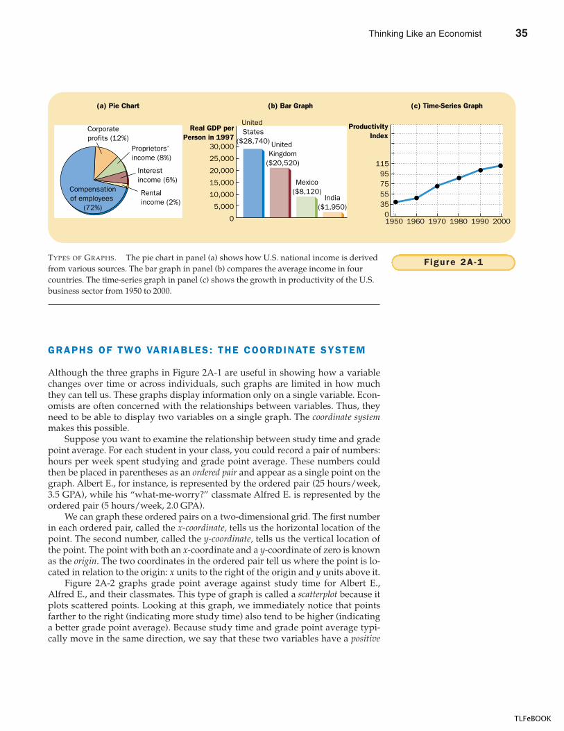
CHAPTER 2 THINKING L IKE AN ECONOMIST 37
GRAPHS OF TWO VARIABLES: THE COORDINATE SYSTEM
Although the three graphs in Figure 2A-1 are useful in showing how a variablechanges over time or across individuals, such graphs are limited in how muchthey can tell us. These graphs display information only on a single variable. Econ-omists are often concerned with the relationships between variables. Thus, theyneed to be able to display two variables on a single graph. The coordinate systemmakes this possible.
Suppose you want to examine the relationship between study time and gradepoint average. For each student in your class, you could record a pair of numbers:hours per week spent studying and grade point average. These numbers couldthen be placed in parentheses as an ordered pair and appear as a single point on thegraph. Albert E., for instance, is represented by the ordered pair (25 hours/week,3.5 GPA), while his “what-me-worry?” classmate Alfred E. is represented by theordered pair (5 hours/week, 2.0 GPA).
We can graph these ordered pairs on a two-dimensional grid. The first numberin each ordered pair, called the x-coordinate, tells us the horizontal location of thepoint. The second number, called the y-coordinate, tells us the vertical location ofthe point. The point with both an x-coordinate and a y-coordinate of zero is knownas the origin. The two coordinates in the ordered pair tell us where the point is lo-cated in relation to the origin: x units to the right of the origin and y units above it.
Figure 2A-2 graphs grade point average against study time for Albert E.,Alfred E., and their classmates. This type of graph is called a scatterplot because itplots scattered points. Looking at this graph, we immediately notice that pointsfarther to the right (indicating more study time) also tend to be higher (indicatinga better grade point average). Because study time and grade point average typi-cally move in the same direction, we say that these two variables have a positive
Rental income (2%)
Corporate profits (12%)
(a) Pie Chart (c) Time-Series Graph
Real GDP perPerson in 1997
United States
($28,740)30,000
25,000
20,000
15,000
10,000
5,000
0
United Kingdom
($20,520)
(b) Bar Graph
Mexico($8,120)
India($1,950)
Compensationof employees
(72%)
Proprietors’ income (8%)
Interest income (6%)
Productivity Index
1159575553501950 1960 1970 1980 1990 2000
Figure 2A-1TYPES OF GRAPHS. The pie chart in panel (a) shows how U.S. national income is derivedfrom various sources. The bar graph in panel (b) compares the average income in fourcountries. The time-series graph in panel (c) shows the growth in productivity of the U.S.business sector from 1950 to 2000.
Thinking Like an Economist 35
TLFeBOOK
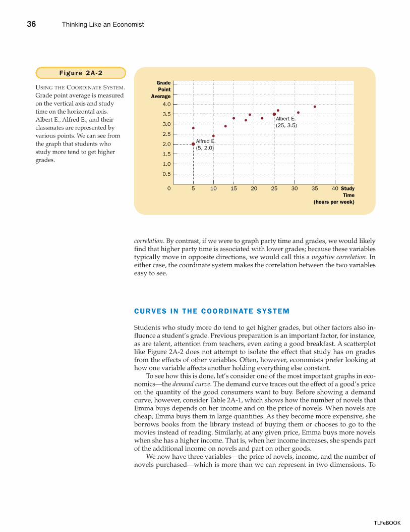
38 PART ONE INTRODUCTION
correlation. By contrast, if we were to graph party time and grades, we would likelyfind that higher party time is associated with lower grades; because these variablestypically move in opposite directions, we would call this a negative correlation. Ineither case, the coordinate system makes the correlation between the two variableseasy to see.
CURVES IN THE COORDINATE SYSTEM
Students who study more do tend to get higher grades, but other factors also in-fluence a student’s grade. Previous preparation is an important factor, for instance,as are talent, attention from teachers, even eating a good breakfast. A scatterplotlike Figure 2A-2 does not attempt to isolate the effect that study has on gradesfrom the effects of other variables. Often, however, economists prefer looking athow one variable affects another holding everything else constant.
To see how this is done, let’s consider one of the most important graphs in eco-nomics—the demand curve. The demand curve traces out the effect of a good’s priceon the quantity of the good consumers want to buy. Before showing a demandcurve, however, consider Table 2A-1, which shows how the number of novels thatEmma buys depends on her income and on the price of novels. When novels arecheap, Emma buys them in large quantities. As they become more expensive, sheborrows books from the library instead of buying them or chooses to go to themovies instead of reading. Similarly, at any given price, Emma buys more novelswhen she has a higher income. That is, when her income increases, she spends partof the additional income on novels and part on other goods.
We now have three variables—the price of novels, income, and the number ofnovels purchased—which is more than we can represent in two dimensions. To
GradePoint
Average
2.5
2.0
1.5
1.0
0.5
40 StudyTime
(hours per week)
3.0
3.5
4.0
0 5 10 15 20 25 30 35
Alfred E.(5, 2.0)
Albert E.(25, 3.5)
Figure 2A-2
USING THE COORDINATE SYSTEM.Grade point average is measuredon the vertical axis and studytime on the horizontal axis.Albert E., Alfred E., and theirclassmates are represented byvarious points. We can see fromthe graph that students whostudy more tend to get highergrades.
36 Thinking Like an Economist
TLFeBOOK
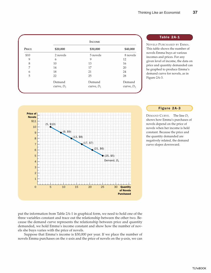
CHAPTER 2 THINKING L IKE AN ECONOMIST 39
put the information from Table 2A-1 in graphical form, we need to hold one of thethree variables constant and trace out the relationship between the other two. Be-cause the demand curve represents the relationship between price and quantitydemanded, we hold Emma’s income constant and show how the number of nov-els she buys varies with the price of novels.
Suppose that Emma’s income is $30,000 per year. If we place the number ofnovels Emma purchases on the x-axis and the price of novels on the y-axis, we can
Table 2A-1
NOVELS PURCHASED BY EMMA.This table shows the number ofnovels Emma buys at variousincomes and prices. For anygiven level of income, the data onprice and quantity demanded canbe graphed to produce Emma’sdemand curve for novels, as inFigure 2A-3.
INCOME
PRICE $20,000 $30,000 $40,000
$10 2 novels 5 novels 8 novels9 6 9 128 10 13 167 14 17 206 18 21 245 22 25 28
Demand Demand Demand curve, D3 curve, D1 curve, D2
Price ofNovels
5
4
3
2
1
30 Quantityof Novels
Purchased
6
7
8
9
10
$11
0 5 10 15 20 25
Demand, D1
(5, $10)
(9, $9)
(13, $8)
(17, $7)
(21, $6)
(25, $5)
Figure 2A-3
DEMAND CURVE. The line D1
shows how Emma’s purchases ofnovels depend on the price ofnovels when her income is heldconstant. Because the price andthe quantity demanded arenegatively related, the demandcurve slopes downward.
Thinking Like an Economist 37
TLFeBOOK
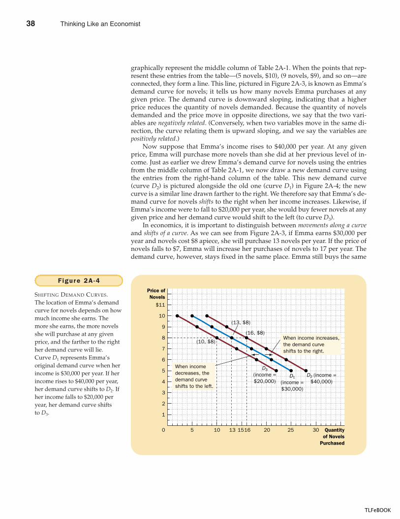
40 PART ONE INTRODUCTION
graphically represent the middle column of Table 2A-1. When the points that rep-resent these entries from the table—(5 novels, $10), (9 novels, $9), and so on—areconnected, they form a line. This line, pictured in Figure 2A-3, is known as Emma’sdemand curve for novels; it tells us how many novels Emma purchases at anygiven price. The demand curve is downward sloping, indicating that a higherprice reduces the quantity of novels demanded. Because the quantity of novelsdemanded and the price move in opposite directions, we say that the two vari-ables are negatively related. (Conversely, when two variables move in the same di-rection, the curve relating them is upward sloping, and we say the variables arepositively related.)
Now suppose that Emma’s income rises to $40,000 per year. At any givenprice, Emma will purchase more novels than she did at her previous level of in-come. Just as earlier we drew Emma’s demand curve for novels using the entriesfrom the middle column of Table 2A-1, we now draw a new demand curve usingthe entries from the right-hand column of the table. This new demand curve(curve D2) is pictured alongside the old one (curve D1) in Figure 2A-4; the newcurve is a similar line drawn farther to the right. We therefore say that Emma’s de-mand curve for novels shifts to the right when her income increases. Likewise, ifEmma’s income were to fall to $20,000 per year, she would buy fewer novels at anygiven price and her demand curve would shift to the left (to curve D3).
In economics, it is important to distinguish between movements along a curveand shifts of a curve. As we can see from Figure 2A-3, if Emma earns $30,000 peryear and novels cost $8 apiece, she will purchase 13 novels per year. If the price ofnovels falls to $7, Emma will increase her purchases of novels to 17 per year. Thedemand curve, however, stays fixed in the same place. Emma still buys the same
Price ofNovels
5
4
3
2
1
30 Quantityof Novels
Purchased
6
7
8
9
10
$11
0 5 13 1610 15 20 25
(13, $8)
(16, $8)
D3
(income =$20,000)
D1
(income =$30,000)
D2 (income =$40,000)
(10, $8)When income increases,the demand curveshifts to the right.
When incomedecreases, thedemand curveshifts to the left.
Figure 2A-4
SHIFTING DEMAND CURVES.The location of Emma’s demandcurve for novels depends on howmuch income she earns. Themore she earns, the more novelsshe will purchase at any givenprice, and the farther to the righther demand curve will lie.Curve D1 represents Emma’soriginal demand curve when herincome is $30,000 per year. If herincome rises to $40,000 per year,her demand curve shifts to D2. Ifher income falls to $20,000 peryear, her demand curve shiftsto D3.
38 Thinking Like an Economist
TLFeBOOK
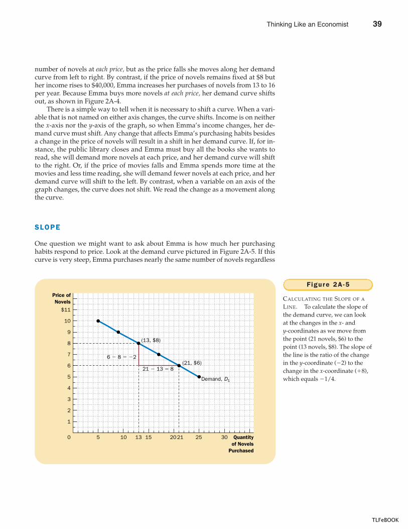
CHAPTER 2 THINKING L IKE AN ECONOMIST 41
number of novels at each price, but as the price falls she moves along her demandcurve from left to right. By contrast, if the price of novels remains fixed at $8 buther income rises to $40,000, Emma increases her purchases of novels from 13 to 16per year. Because Emma buys more novels at each price, her demand curve shiftsout, as shown in Figure 2A-4.
There is a simple way to tell when it is necessary to shift a curve. When a vari-able that is not named on either axis changes, the curve shifts. Income is on neitherthe x-axis nor the y-axis of the graph, so when Emma’s income changes, her de-mand curve must shift. Any change that affects Emma’s purchasing habits besidesa change in the price of novels will result in a shift in her demand curve. If, for in-stance, the public library closes and Emma must buy all the books she wants toread, she will demand more novels at each price, and her demand curve will shiftto the right. Or, if the price of movies falls and Emma spends more time at themovies and less time reading, she will demand fewer novels at each price, and herdemand curve will shift to the left. By contrast, when a variable on an axis of thegraph changes, the curve does not shift. We read the change as a movement alongthe curve.
SLOPE
One question we might want to ask about Emma is how much her purchasinghabits respond to price. Look at the demand curve pictured in Figure 2A-5. If thiscurve is very steep, Emma purchases nearly the same number of novels regardless
Price ofNovels
5
4
3
2
1
30 Quantityof Novels
Purchased
6
7
8
9
10
$11
0 5 211310 15 20 25
Demand, D1
(13, $8)
(21, $6)6 � 8 � �2
21 � 13 � 8
Figure 2A-5
CALCULATING THE SLOPE OF A
LINE. To calculate the slope ofthe demand curve, we can lookat the changes in the x- andy-coordinates as we move fromthe point (21 novels, $6) to thepoint (13 novels, $8). The slope ofthe line is the ratio of the changein the y-coordinate (�2) to thechange in the x-coordinate (�8),which equals �1/4.
Thinking Like an Economist 39
TLFeBOOK
42 PART ONE INTRODUCTION
of whether they are cheap or expensive. If this curve is much flatter, Emma pur-chases many fewer novels when the price rises. To answer questions about howmuch one variable responds to changes in another variable, we can use the con-cept of slope.
The slope of a line is the ratio of the vertical distance covered to the horizontaldistance covered as we move along the line. This definition is usually written outin mathematical symbols as follows:
slope = ,
where the Greek letter ∆ (delta) stands for the change in a variable. In other words,the slope of a line is equal to the “rise” (change in y) divided by the “run” (changein x). The slope will be a small positive number for a fairly flat upward-sloping line,a large positive number for a steep upward-sloping line, and a negative numberfor a downward-sloping line. A horizontal line has a slope of zero because inthis case the y-variable never changes; a vertical line is defined to have an infiniteslope because the y-variable can take any value without the x-variable changingat all.
What is the slope of Emma’s demand curve for novels? First of all, because thecurve slopes down, we know the slope will be negative. To calculate a numericalvalue for the slope, we must choose two points on the line. With Emma’s incomeat $30,000, she will purchase 21 novels at a price of $6 or 13 novels at a price of $8.When we apply the slope formula, we are concerned with the change betweenthese two points; in other words, we are concerned with the difference betweenthem, which lets us know that we will have to subtract one set of values from theother, as follows:
slope = = = = = .
Figure 2A-5 shows graphically how this calculation works. Try computing theslope of Emma’s demand curve using two different points. You should get exactlythe same result, �1/4. One of the properties of a straight line is that it has the sameslope everywhere. This is not true of other types of curves, which are steeper insome places than in others.
The slope of Emma’s demand curve tells us something about how responsiveher purchases are to changes in the price. A small slope (a number close to zero)means that Emma’s demand curve is relatively flat; in this case, she adjusts thenumber of novels she buys substantially in response to a price change. A largerslope (a number farther from zero) means that Emma’s demand curve is relativelysteep; in this case, she adjusts the number of novels she buys only slightly in re-sponse to a price change.
CAUSE AND EFFECT
Economists often use graphs to advance an argument about how the economyworks. In other words, they use graphs to argue about how one set of eventscauses another set of events. With a graph like the demand curve, there is nodoubt about cause and effect. Because we are varying price and holding all other
�14
�28
6�821�13
first y-coordinate�second y-coordinatefirst x-coordinate�second x-coordinate
�y
�x
�y
�x
40 Thinking Like an Economist
TLFeBOOK
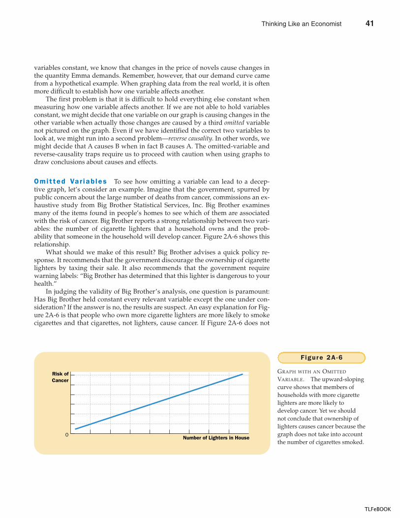
CHAPTER 2 THINKING L IKE AN ECONOMIST 43
variables constant, we know that changes in the price of novels cause changes inthe quantity Emma demands. Remember, however, that our demand curve camefrom a hypothetical example. When graphing data from the real world, it is oftenmore difficult to establish how one variable affects another.
The first problem is that it is difficult to hold everything else constant whenmeasuring how one variable affects another. If we are not able to hold variablesconstant, we might decide that one variable on our graph is causing changes in theother variable when actually those changes are caused by a third omitted variablenot pictured on the graph. Even if we have identified the correct two variables tolook at, we might run into a second problem—reverse causality. In other words, wemight decide that A causes B when in fact B causes A. The omitted-variable andreverse-causality traps require us to proceed with caution when using graphs todraw conclusions about causes and effects.
Omit ted Var iab les To see how omitting a variable can lead to a decep-tive graph, let’s consider an example. Imagine that the government, spurred bypublic concern about the large number of deaths from cancer, commissions an ex-haustive study from Big Brother Statistical Services, Inc. Big Brother examinesmany of the items found in people’s homes to see which of them are associatedwith the risk of cancer. Big Brother reports a strong relationship between two vari-ables: the number of cigarette lighters that a household owns and the prob-ability that someone in the household will develop cancer. Figure 2A-6 shows thisrelationship.
What should we make of this result? Big Brother advises a quick policy re-sponse. It recommends that the government discourage the ownership of cigarettelighters by taxing their sale. It also recommends that the government requirewarning labels: “Big Brother has determined that this lighter is dangerous to yourhealth.”
In judging the validity of Big Brother’s analysis, one question is paramount:Has Big Brother held constant every relevant variable except the one under con-sideration? If the answer is no, the results are suspect. An easy explanation for Fig-ure 2A-6 is that people who own more cigarette lighters are more likely to smokecigarettes and that cigarettes, not lighters, cause cancer. If Figure 2A-6 does not
Risk ofCancer
Number of Lighters in House0
Figure 2A-6
GRAPH WITH AN OMITTED
VARIABLE. The upward-slopingcurve shows that members ofhouseholds with more cigarettelighters are more likely todevelop cancer. Yet we shouldnot conclude that ownership oflighters causes cancer because thegraph does not take into accountthe number of cigarettes smoked.
Thinking Like an Economist 41
TLFeBOOK
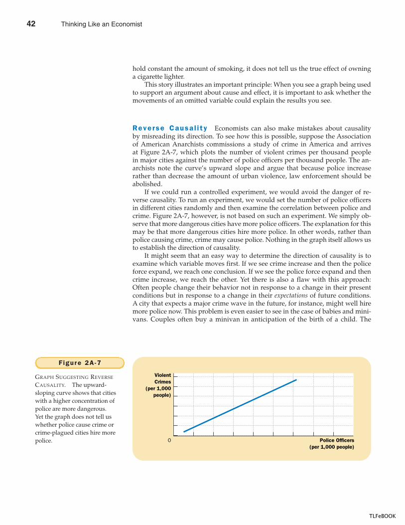
44 PART ONE INTRODUCTION
hold constant the amount of smoking, it does not tell us the true effect of owninga cigarette lighter.
This story illustrates an important principle: When you see a graph being usedto support an argument about cause and effect, it is important to ask whether themovements of an omitted variable could explain the results you see.
Reverse Causa l i t y Economists can also make mistakes about causalityby misreading its direction. To see how this is possible, suppose the Associationof American Anarchists commissions a study of crime in America and arrivesat Figure 2A-7, which plots the number of violent crimes per thousand peoplein major cities against the number of police officers per thousand people. The an-archists note the curve’s upward slope and argue that because police increaserather than decrease the amount of urban violence, law enforcement should beabolished.
If we could run a controlled experiment, we would avoid the danger of re-verse causality. To run an experiment, we would set the number of police officersin different cities randomly and then examine the correlation between police andcrime. Figure 2A-7, however, is not based on such an experiment. We simply ob-serve that more dangerous cities have more police officers. The explanation for thismay be that more dangerous cities hire more police. In other words, rather thanpolice causing crime, crime may cause police. Nothing in the graph itself allows usto establish the direction of causality.
It might seem that an easy way to determine the direction of causality is toexamine which variable moves first. If we see crime increase and then the policeforce expand, we reach one conclusion. If we see the police force expand and thencrime increase, we reach the other. Yet there is also a flaw with this approach:Often people change their behavior not in response to a change in their presentconditions but in response to a change in their expectations of future conditions.A city that expects a major crime wave in the future, for instance, might well hiremore police now. This problem is even easier to see in the case of babies and mini-vans. Couples often buy a minivan in anticipation of the birth of a child. The
ViolentCrimes
(per 1,000people)
Police Officers(per 1,000 people)
0
Figure 2A-7
GRAPH SUGGESTING REVERSE
CAUSALITY. The upward-sloping curve shows that citieswith a higher concentration ofpolice are more dangerous.Yet the graph does not tell uswhether police cause crime orcrime-plagued cities hire morepolice.
42 Thinking Like an Economist
TLFeBOOK
CHAPTER 2 THINKING L IKE AN ECONOMIST 45
minivan comes before the baby, but we wouldn’t want to conclude that the saleof minivans causes the population to grow!
There is no complete set of rules that says when it is appropriate to drawcausal conclusions from graphs. Yet just keeping in mind that cigarette lightersdon’t cause cancer (omitted variable) and minivans don’t cause larger fam-ilies (reverse causality) will keep you from falling for many faulty economicarguments.
Thinking Like an Economist 43
TLFeBOOK

TLFeBOOK
IN THIS CHAPTERYOU WILL . . .
See how comparat iveadvantage exp la ins
the ga ins f r om t rade
Cons ider however yone can benef i t
when peop le t radewith one another
Learn the meaning o fabso lute advantage
and comparat iveadvantage
Apply the theor y o fcomparat iveadvantage to
ever yday l i fe andnat iona l po l icy
Consider your typical day. You wake up in the morning, and you pour yourselfjuice from oranges grown in Florida and coffee from beans grown in Brazil. Overbreakfast, you watch a news program broadcast from New York on your televisionmade in Japan. You get dressed in clothes made of cotton grown in Georgia andsewn in factories in Thailand. You drive to class in a car made of parts manufac-tured in more than a dozen countries around the world. Then you open up youreconomics textbook written by an author living in Massachusetts, published by acompany located in Texas, and printed on paper made from trees grown in Oregon.
Every day you rely on many people from around the world, most of whom youdo not know, to provide you with the goods and services that you enjoy. Such inter-dependence is possible because people trade with one another. Those people whoprovide you with goods and services are not acting out of generosity or concern foryour welfare. Nor is some government agency directing them to make what you
I N T E R D E P E N D E N C E A N D T H E
G A I N S F R O M T R A D E
47
45
3
TLFeBOOK
48 PART ONE INTRODUCTION
want and to give it to you. Instead, people provide you and other consumers withthe goods and services they produce because they get something in return.
In subsequent chapters we will examine how our economy coordinates the ac-tivities of millions of people with varying tastes and abilities. As a starting pointfor this analysis, here we consider the reasons for economic interdependence. Oneof the Ten Principles of Economics highlighted in Chapter 1 is that trade can makeeveryone better off. This principle explains why people trade with their neighborsand why nations trade with other nations. In this chapter we examine this princi-ple more closely. What exactly do people gain when they trade with one another?Why do people choose to become interdependent?
A PARABLE FOR THE MODERN ECONOMY
To understand why people choose to depend on others for goods and services andhow this choice improves their lives, let’s look at a simple economy. Imagine thatthere are two goods in the world—meat and potatoes. And there are two people inthe world—a cattle rancher and a potato farmer—each of whom would like to eatboth meat and potatoes.
The gains from trade are most obvious if the rancher can produce only meatand the farmer can produce only potatoes. In one scenario, the rancher and thefarmer could choose to have nothing to do with each other. But after severalmonths of eating beef roasted, boiled, broiled, and grilled, the rancher might de-cide that self-sufficiency is not all it’s cracked up to be. The farmer, who has beeneating potatoes mashed, fried, baked, and scalloped, would likely agree. It is easyto see that trade would allow them to enjoy greater variety: Each could then havea hamburger with french fries.
Although this scene illustrates most simply how everyone can benefit fromtrade, the gains would be similar if the rancher and the farmer were each capableof producing the other good, but only at great cost. Suppose, for example, that thepotato farmer is able to raise cattle and produce meat, but that he is not very goodat it. Similarly, suppose that the cattle rancher is able to grow potatoes, but that herland is not very well suited for it. In this case, it is easy to see that the farmer andthe rancher can each benefit by specializing in what he or she does best and thentrading with the other.
The gains from trade are less obvious, however, when one person is better atproducing every good. For example, suppose that the rancher is better at raisingcattle and better at growing potatoes than the farmer. In this case, should therancher or farmer choose to remain self-sufficient? Or is there still reason for themto trade with each other? To answer this question, we need to look more closely atthe factors that affect such a decision.
PRODUCTION POSSIBIL IT IES
Suppose that the farmer and the rancher each work 40 hours a week and can de-vote this time to growing potatoes, raising cattle, or a combination of the two.Table 3-1 shows the amount of time each person requires to produce 1 pound of
46 Interdependence and the Gains from Trade
TLFeBOOK
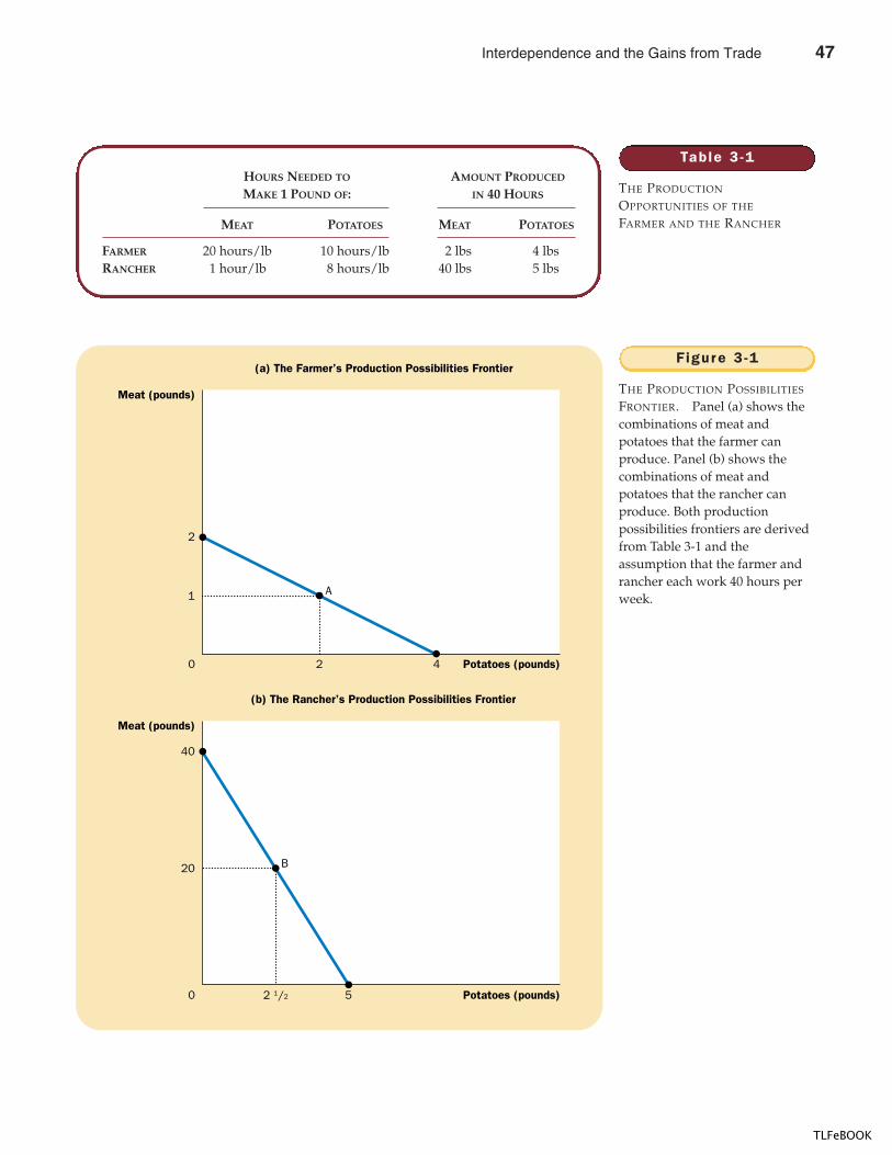
CHAPTER 3 INTERDEPENDENCE AND THE GAINS FROM TRADE 49
Tab le 3 -1
THE PRODUCTION
OPPORTUNITIES OF THE
FARMER AND THE RANCHER
HOURS NEEDED TO AMOUNT PRODUCED
MAKE 1 POUND OF: IN 40 HOURS
MEAT POTATOES MEAT POTATOES
FARMER 20 hours/lb 10 hours/lb 2 lbs 4 lbsRANCHER 1 hour/lb 8 hours/lb 40 lbs 5 lbs
1
2
Potatoes (pounds)2 4
A
0
Meat (pounds)
(a) The Farmer’s Production Possibilities Frontier
20
Potatoes (pounds)2 1/2
B
0
Meat (pounds)
(b) The Rancher’s Production Possibilities Frontier
5
40
Figure 3 -1
THE PRODUCTION POSSIBILITIES
FRONTIER. Panel (a) shows thecombinations of meat andpotatoes that the farmer canproduce. Panel (b) shows thecombinations of meat andpotatoes that the rancher canproduce. Both productionpossibilities frontiers are derivedfrom Table 3-1 and theassumption that the farmer andrancher each work 40 hours perweek.
Interdependence and the Gains from Trade 47
TLFeBOOK
50 PART ONE INTRODUCTION
each good. The farmer can produce a pound of potatoes in 10 hours and a poundof meat in 20 hours. The rancher, who is more productive in both activities, canproduce a pound of potatoes in 8 hours and a pound of meat in 1 hour.
Panel (a) of Figure 3-1 illustrates the amounts of meat and potatoes that thefarmer can produce. If the farmer devotes all 40 hours of his time to potatoes, heproduces 4 pounds of potatoes and no meat. If he devotes all his time to meat, heproduces 2 pounds of meat and no potatoes. If the farmer divides his time equallybetween the two activities, spending 20 hours on each, he produces 2 pounds ofpotatoes and 1 pound of meat. The figure shows these three possible outcomes andall others in between.
This graph is the farmer’s production possibilities frontier. As we discussed inChapter 2, a production possibilities frontier shows the various mixes of outputthat an economy can produce. It illustrates one of the Ten Principles of Economics inChapter 1: People face tradeoffs. Here the farmer faces a tradeoff between produc-ing meat and producing potatoes. You may recall that the production possibilitiesfrontier in Chapter 2 was drawn bowed out; in this case, the tradeoff between thetwo goods depends on the amounts being produced. Here, however, the farmer’stechnology for producing meat and potatoes (as summarized in Table 3-1) allowshim to switch between one good and the other at a constant rate. In this case, theproduction possibilities frontier is a straight line.
Panel (b) of Figure 3-1 shows the production possibilities frontier for therancher. If the rancher devotes all 40 hours of her time to potatoes, she produces 5pounds of potatoes and no meat. If she devotes all her time to meat, she produces40 pounds of meat and no potatoes. If the rancher divides her time equally, spend-ing 20 hours on each activity, she produces 2 1/2 pounds of potatoes and 20pounds of meat. Once again, the production possibilities frontier shows all thepossible outcomes.
If the farmer and rancher choose to be self-sufficient, rather than trade witheach other, then each consumes exactly what he or she produces. In this case, theproduction possibilities frontier is also the consumption possibilities frontier. Thatis, without trade, Figure 3-1 shows the possible combinations of meat and potatoesthat the farmer and rancher can each consume.
Although these production possibilities frontiers are useful in showing thetradeoffs that the farmer and rancher face, they do not tell us what the farmer andrancher will actually choose to do. To determine their choices, we need to knowthe tastes of the farmer and the rancher. Let’s suppose they choose the combina-tions identified by points A and B in Figure 3-1: The farmer produces and con-sumes 2 pounds of potatoes and 1 pound of meat, while the rancher produces andconsumes 2 1/2 pounds of potatoes and 20 pounds of meat.
SPECIALIZATION AND TRADE
After several years of eating combination B, the rancher gets an idea and goes totalk to the farmer:
RANCHER: Farmer, my friend, have I got a deal for you! I know how to improvelife for both of us. I think you should stop producing meat altogetherand devote all your time to growing potatoes. According to mycalculations, if you work 40 hours a week growing potatoes, you’ll
48 Interdependence and the Gains from Trade
TLFeBOOK
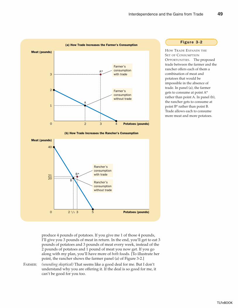
CHAPTER 3 INTERDEPENDENCE AND THE GAINS FROM TRADE 51
produce 4 pounds of potatoes. If you give me 1 of those 4 pounds,I’ll give you 3 pounds of meat in return. In the end, you’ll get to eat 3pounds of potatoes and 3 pounds of meat every week, instead of the2 pounds of potatoes and 1 pound of meat you now get. If you goalong with my plan, you’ll have more of both foods. [To illustrate herpoint, the rancher shows the farmer panel (a) of Figure 3-2.]
FARMER: (sounding skeptical) That seems like a good deal for me. But I don’tunderstand why you are offering it. If the deal is so good for me, itcan’t be good for you too.
1
2
3
Potatoes (pounds)2 3 4
A
0
Meat (pounds)
(a) How Trade Increases the Farmer’s Consumption
A*
Farmer’sconsumptionwith trade
Farmer’sconsumptionwithout trade
2021
Potatoes (pounds)2 1/2
B
0
Meat (pounds)
(b) How Trade Increases the Rancher’s Consumption
53
B*
40
Rancher’sconsumptionwithout trade
Rancher’sconsumptionwith trade
Figure 3 -2
HOW TRADE EXPANDS THE
SET OF CONSUMPTION
OPPORTUNITIES. The proposedtrade between the farmer and therancher offers each of them acombination of meat andpotatoes that would beimpossible in the absence oftrade. In panel (a), the farmergets to consume at point A*rather than point A. In panel (b),the rancher gets to consume atpoint B* rather than point B.Trade allows each to consumemore meat and more potatoes.
Interdependence and the Gains from Trade 49
TLFeBOOK
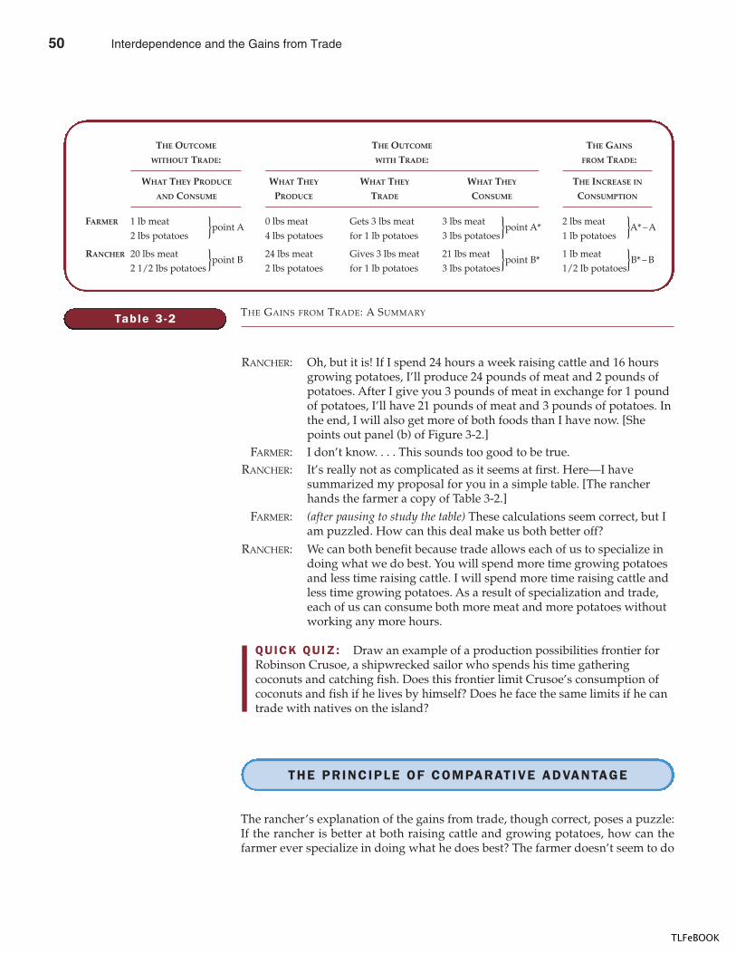
52 PART ONE INTRODUCTION
RANCHER: Oh, but it is! If I spend 24 hours a week raising cattle and 16 hoursgrowing potatoes, I’ll produce 24 pounds of meat and 2 pounds ofpotatoes. After I give you 3 pounds of meat in exchange for 1 poundof potatoes, I’ll have 21 pounds of meat and 3 pounds of potatoes. Inthe end, I will also get more of both foods than I have now. [Shepoints out panel (b) of Figure 3-2.]
FARMER: I don’t know. . . . This sounds too good to be true.RANCHER: It’s really not as complicated as it seems at first. Here—I have
summarized my proposal for you in a simple table. [The rancherhands the farmer a copy of Table 3-2.]
FARMER: (after pausing to study the table) These calculations seem correct, but Iam puzzled. How can this deal make us both better off?
RANCHER: We can both benefit because trade allows each of us to specialize indoing what we do best. You will spend more time growing potatoesand less time raising cattle. I will spend more time raising cattle andless time growing potatoes. As a result of specialization and trade,each of us can consume both more meat and more potatoes withoutworking any more hours.
QUICK QUIZ: Draw an example of a production possibilities frontier forRobinson Crusoe, a shipwrecked sailor who spends his time gatheringcoconuts and catching fish. Does this frontier limit Crusoe’s consumption ofcoconuts and fish if he lives by himself? Does he face the same limits if he cantrade with natives on the island?
THE PRINCIPLE OF COMPARATIVE ADVANTAGE
The rancher’s explanation of the gains from trade, though correct, poses a puzzle:If the rancher is better at both raising cattle and growing potatoes, how can thefarmer ever specialize in doing what he does best? The farmer doesn’t seem to do
Table 3 -2
THE OUTCOME THE OUTCOME THE GAINS
WITHOUT TRADE: WITH TRADE: FROM TRADE:
WHAT THEY PRODUCE WHAT THEY WHAT THEY WHAT THEY THE INCREASE IN
AND CONSUME PRODUCE TRADE CONSUME CONSUMPTION
FARMER 1 lb meat 0 lbs meat Gets 3 lbs meat 3 lbs meat 2 lbs meat2 lbs potatoes 4 lbs potatoes for 1 lb potatoes 3 lbs potatoes 1 lb potatoes
RANCHER 20 lbs meat 24 lbs meat Gives 3 lbs meat 21 lbs meat 1 lb meat2 1/2 lbs potatoes 2 lbs potatoes for 1 lb potatoes 3 lbs potatoes 1/2 lb potatoes
THE GAINS FROM TRADE: A SUMMARY
}point A }point A* }A* –A
}point B }point B* }B* – B
50 Interdependence and the Gains from Trade
TLFeBOOK
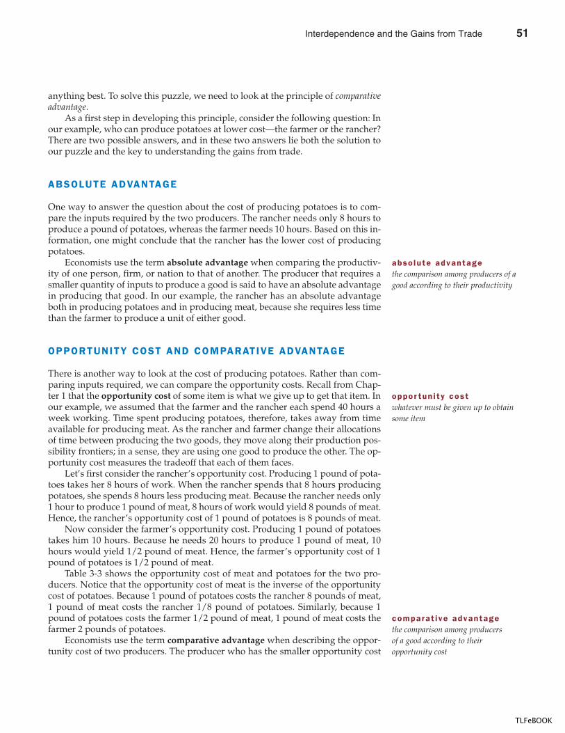
CHAPTER 3 INTERDEPENDENCE AND THE GAINS FROM TRADE 53
anything best. To solve this puzzle, we need to look at the principle of comparativeadvantage.
As a first step in developing this principle, consider the following question: Inour example, who can produce potatoes at lower cost—the farmer or the rancher?There are two possible answers, and in these two answers lie both the solution toour puzzle and the key to understanding the gains from trade.
ABSOLUTE ADVANTAGE
One way to answer the question about the cost of producing potatoes is to com-pare the inputs required by the two producers. The rancher needs only 8 hours toproduce a pound of potatoes, whereas the farmer needs 10 hours. Based on this in-formation, one might conclude that the rancher has the lower cost of producingpotatoes.
Economists use the term absolute advantage when comparing the productiv-ity of one person, firm, or nation to that of another. The producer that requires asmaller quantity of inputs to produce a good is said to have an absolute advantagein producing that good. In our example, the rancher has an absolute advantageboth in producing potatoes and in producing meat, because she requires less timethan the farmer to produce a unit of either good.
OPPORTUNITY COST AND COMPARATIVE ADVANTAGE
There is another way to look at the cost of producing potatoes. Rather than com-paring inputs required, we can compare the opportunity costs. Recall from Chap-ter 1 that the opportunity cost of some item is what we give up to get that item. Inour example, we assumed that the farmer and the rancher each spend 40 hours aweek working. Time spent producing potatoes, therefore, takes away from timeavailable for producing meat. As the rancher and farmer change their allocationsof time between producing the two goods, they move along their production pos-sibility frontiers; in a sense, they are using one good to produce the other. The op-portunity cost measures the tradeoff that each of them faces.
Let’s first consider the rancher’s opportunity cost. Producing 1 pound of pota-toes takes her 8 hours of work. When the rancher spends that 8 hours producingpotatoes, she spends 8 hours less producing meat. Because the rancher needs only1 hour to produce 1 pound of meat, 8 hours of work would yield 8 pounds of meat.Hence, the rancher’s opportunity cost of 1 pound of potatoes is 8 pounds of meat.
Now consider the farmer’s opportunity cost. Producing 1 pound of potatoestakes him 10 hours. Because he needs 20 hours to produce 1 pound of meat, 10hours would yield 1/2 pound of meat. Hence, the farmer’s opportunity cost of 1pound of potatoes is 1/2 pound of meat.
Table 3-3 shows the opportunity cost of meat and potatoes for the two pro-ducers. Notice that the opportunity cost of meat is the inverse of the opportunitycost of potatoes. Because 1 pound of potatoes costs the rancher 8 pounds of meat,1 pound of meat costs the rancher 1/8 pound of potatoes. Similarly, because 1pound of potatoes costs the farmer 1/2 pound of meat, 1 pound of meat costs thefarmer 2 pounds of potatoes.
Economists use the term comparative advantage when describing the oppor-tunity cost of two producers. The producer who has the smaller opportunity cost
abso lute advantagethe comparison among producers of agood according to their productivity
oppor tun i ty costwhatever must be given up to obtainsome item
comparat ive advantagethe comparison among producersof a good according to theiropportunity cost
Interdependence and the Gains from Trade 51
TLFeBOOK
54 PART ONE INTRODUCTION
of producing a good—that is, who has to give up less of other goods to produceit—is said to have a comparative advantage in producing that good. In our exam-ple, the farmer has a lower opportunity cost of producing potatoes than therancher (1/2 pound versus 8 pounds of meat). The rancher has a lower opportu-nity cost of producing meat than the farmer (1/8 pound versus 2 pounds of pota-toes). Thus, the farmer has a comparative advantage in growing potatoes, and therancher has a comparative advantage in producing meat.
Notice that it would be impossible for the same person to have a comparativeadvantage in both goods. Because the opportunity cost of one good is the inverseof the opportunity cost of the other, if a person’s opportunity cost of one good isrelatively high, his opportunity cost of the other good must be relatively low. Com-parative advantage reflects the relative opportunity cost. Unless two people haveexactly the same opportunity cost, one person will have a comparative advantagein one good, and the other person will have a comparative advantage in the othergood.
COMPARATIVE ADVANTAGE AND TRADE
Differences in opportunity cost and comparative advantage create the gains fromtrade. When each person specializes in producing the good for which he or she hasa comparative advantage, total production in the economy rises, and this increasein the size of the economic pie can be used to make everyone better off. In otherwords, as long as two people have different opportunity costs, each can benefitfrom trade by obtaining a good at a price lower than his or her opportunity cost ofthat good.
Consider the proposed deal from the viewpoint of the farmer. The farmer gets3 pounds of meat in exchange for 1 pound of potatoes. In other words, the farmerbuys each pound of meat for a price of 1/3 pound of potatoes. This price of meatis lower than his opportunity cost for 1 pound of meat, which is 2 pounds of pota-toes. Thus, the farmer benefits from the deal because he gets to buy meat at a goodprice.
Now consider the deal from the rancher’s viewpoint. The rancher buys 1pound of potatoes for a price of 3 pounds of meat. This price of potatoes is lowerthan her opportunity cost of 1 pound of potatoes, which is 8 pounds of meat. Thus,the rancher benefits because she gets to buy potatoes at a good price.
These benefits arise because each person concentrates on the activity for whichhe or she has the lower opportunity cost: The farmer spends more time growingpotatoes, and the rancher spends more time producing meat. As a result, the totalproduction of potatoes and the total production of meat both rise, and the farmer
Table 3 -3
THE OPPORTUNITY COST OF
MEAT AND POTATOES
OPPORTUNITY COST OF:
1 POUND OF MEAT 1 POUND OF POTATOES
FARMER 2 lbs potatoes 1/2 lb meatRANCHER 1/8 lb potatoes 8 lbs meat
52 Interdependence and the Gains from Trade
TLFeBOOK
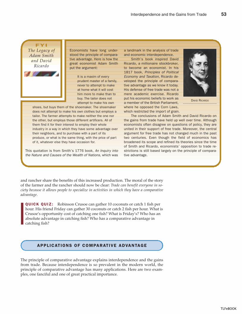
CHAPTER 3 INTERDEPENDENCE AND THE GAINS FROM TRADE 55
and rancher share the benefits of this increased production. The moral of the storyof the farmer and the rancher should now be clear: Trade can benefit everyone in so-ciety because it allows people to specialize in activities in which they have a comparativeadvantage.
QUICK QUIZ: Robinson Crusoe can gather 10 coconuts or catch 1 fish perhour. His friend Friday can gather 30 coconuts or catch 2 fish per hour. What isCrusoe’s opportunity cost of catching one fish? What is Friday’s? Who has anabsolute advantage in catching fish? Who has a comparative advantage incatching fish?
APPLICATIONS OF COMPARATIVE ADVANTAGE
The principle of comparative advantage explains interdependence and the gainsfrom trade. Because interdependence is so prevalent in the modern world, theprinciple of comparative advantage has many applications. Here are two exam-ples, one fanciful and one of great practical importance.
Economists have long under-stood the principle of compara-tive advantage. Here is how thegreat economist Adam Smithput the argument:
It is a maxim of everyprudent master of a family,never to attempt to makeat home what it will costhim more to make than tobuy. The tailor does notattempt to make his own
shoes, but buys them of the shoemaker. The shoemakerdoes not attempt to make his own clothes but employs atailor. The farmer attempts to make neither the one northe other, but employs those different artificers. All ofthem find it for their interest to employ their wholeindustry in a way in which they have some advantage overtheir neighbors, and to purchase with a part of itsproduce, or what is the same thing, with the price of partof it, whatever else they have occasion for.
This quotation is from Smith’s 1776 book, An Inquiry intothe Nature and Causes of the Wealth of Nations, which was
a landmark in the analysis of tradeand economic interdependence.
Smith’s book inspired DavidRicardo, a millionaire stockbroker,to become an economist. In his1817 book, Principles of PoliticalEconomy and Taxation, Ricardo de-veloped the principle of compara-tive advantage as we know it today.His defense of free trade was not amere academic exercise. Ricardoput his economic beliefs to work asa member of the British Parliament,where he opposed the Corn Laws,which restricted the import of grain.
The conclusions of Adam Smith and David Ricardo onthe gains from trade have held up well over time. Althougheconomists often disagree on questions of policy, they areunited in their support of free trade. Moreover, the centralargument for free trade has not changed much in the pasttwo centuries. Even though the field of economics hasbroadened its scope and refined its theories since the timeof Smith and Ricardo, economists’ opposition to trade re-strictions is still based largely on the principle of compara-tive advantage.
DAVID RICARDO
FYIThe Legacy ofAdam Smithand David
Ricardo
Interdependence and the Gains from Trade 53
TLFeBOOK
56 PART ONE INTRODUCTION
SHOULD T IGER WOODS MOW HIS OWN LAWN?
Tiger Woods spends a lot of time walking around on grass. One of the most tal-ented golfers of all time, he can hit a drive and sink a putt in a way that most ca-sual golfers only dream of doing. Most likely, he is talented at other activities too.For example, let’s imagine that Woods can mow his lawn faster than anyone else.But just because he can mow his lawn fast, does this mean he should?
To answer this question, we can use the concepts of opportunity cost and com-parative advantage. Let’s say that Woods can mow his lawn in 2 hours. In that same2 hours, he could film a television commercial for Nike and earn $10,000. By con-trast, Forrest Gump, the boy next door, can mow Woods’s lawn in 4 hours. In thatsame 4 hours, he could work at McDonald’s and earn $20.
In this example, Woods’s opportunity cost of mowing the lawn is $10,000 andForrest’s opportunity cost is $20. Woods has an absolute advantage in mowinglawns because he can do the work in less time. Yet Forrest has a comparative ad-vantage in mowing lawns because he has the lower opportunity cost.
A COMMON BARRIER TO FREE TRADE
among countries is tariffs, which aretaxes on the import of goods fromabroad. In the following opinion col-umn, economist Douglas Irwin dis-cusses a recent example of their use.
L a m b Ta r i f f s F l e e c eU . S . C o n s u m e r s
BY DOUGLAS A. IRWIN
President Clinton dealt a serious blow tofree trade last Wednesday, when he an-nounced that the U.S. would impose stiffimport tariffs on lamb from Australia andNew Zealand. His decision undercuts
American leadership and makes a mock-ery of the administration’s claims that itfavors free and fair trade.
U.S. sheep producers have longbeen dependent on government. Formore than half a century, until Congressenacted farm-policy reforms in 1995,they received subsidies for wool. Havinglost that handout, saddled with highcosts and inefficiencies, and facing do-mestic competition from chicken, beef,and pork, sheep producers sought tostop foreign competition by filing for im-port relief.
Almost all U.S. lamb imports comefrom Australia and New Zealand, majoragricultural producers with a crushingcomparative advantage. New Zealandhas fewer than four million people but asmany as 60 million sheep (comparedwith about seven million sheep in theU.S.). New Zealand’s farmers have in-vested substantial resources in newtechnology and effective marketing,making them among the most efficientproducers in the world. New Zealandalso eliminated domestic agricultural
subsidies in the free-market reforms ofthe 1950s, and is a free-trading country,on track to eliminate all import tariffs by2006.
Rather than emulate this example,the American Sheep Industry Asso-ciation, among others, filed an “escapeclause” petition under the Trade Actof 1974, which allows temporary“breathing space” protection to import-competing industries. Under the escape-clause provision, a petitioning industry isrequired to present an adjustment planto ensure that it undertakes steps to be-come competitive in the future. The tariffprotection is usually limited and sched-uled to be phased out.
The U.S. International Trade Com-mission determines whether imports area cause of “serious injury” to the do-mestic industry and, if so, proposes aremedy, which the president has full dis-cretion to adopt, change or reject. InFebruary, the ITC did not find that the do-mestic industry had suffered “serious in-jury,” but rather adopted the weakerruling that imports were “a substantial
IN THE NEWSWho has a Comparative
Advantage inProducing Lamb?
54 Interdependence and the Gains from Trade
TLFeBOOK
CHAPTER 3 INTERDEPENDENCE AND THE GAINS FROM TRADE 57
The gains from trade in this example are tremendous. Rather than mowing hisown lawn, Woods should make the commercial and hire Forrest to mow the lawn.As long as Woods pays Forrest more than $20 and less than $10,000, both of themare better off.
SHOULD THE UNITED STATES TRADEWITH OTHER COUNTRIES?
Just as individuals can benefit from specialization and trade with one another, asthe farmer and rancher did, so can populations of people in different countries.Many of the goods that Americans enjoy are produced abroad, and many of thegoods produced in the United States are sold abroad. Goods produced abroad andsold domestically are called imports. Goods produced domestically and soldabroad are called exports.
cause of threat of serious injury.” TheITC did not propose to roll back imports,only to impose a 20% tariff (decliningover four years) on imports above lastyear’s levels.
The administration at first appearedto be considering less restrictive mea-sures. Australia and New Zealand evenoffered financial assistance to the U.S.producers, and the administration de-layed any announcement and appearedto be working toward a compromise. Butthese hopes were completely dashedwith the shocking final decision, in whichthe administration capitulated to the de-mands of the sheep industry and its ad-vocates in Congress.
The congressional charge was ledby Sen. Max Baucus (D., Mont.), amember of the Agriculture Committeewhose sister, a sheep producer, had ap-peared before the ITC to press for highertariffs. The administration opted for . . .[the following:] On top of existing tariffs,the president imposed a 9% tariff on allimports in the first year (declining to 6%and then 3% in years two and three), and
a whopping 40% tariff on imports abovelast year’s levels (dropping to 32% and24%). . . .
The American Sheep Industry Asso-ciation’s president happily announcedthat the move will “bring some stabilityto the market.” Whenever producersspeak of bringing stability to the market,you know that consumers are gettingfleeced.
The lamb decision, while little no-ticed at home, has been closely followedabroad. The decision undercuts the ad-ministration’s free-trade rhetoric andharms its efforts to get other countriesto open up their markets. Some importrelief had been expected, but not soclearly protectionist as what finally mate-rialized. The extreme decision has out-raged farmers in Australia and NewZealand, and officials there have vowedto take the U.S. to a WTO dispute set-tlement panel.
The administration’s timing couldnot have been worse. The decision cameright after an Asia Pacific Economic Co-operation summit reaffirmed its commit-
ment to reduce trade barriers, and a fewmonths before the World Trade Organi-zation’s November meeting in Seattle,where the WTO is to launch a new roundof multilateral trade negotiations. A prin-cipal U.S. objective at the summit is thereduction of agricultural protection in Eu-rope and elsewhere.
In 1947, facing an election the nextyear, President Truman courageously re-sisted special interest pressure and ve-toed a bill to impose import quotas onwool, which would have jeopardized thefirst postwar multilateral trade negotia-tions due to start later that year. In con-trast, Mr. Clinton, though a lame duck,caved in to political pressure. If the U.S.,whose booming economy is the envy ofthe world, cannot resist protectionism,how can it expect other countries todo so?
SOURCE: The Wall Street Journal, July 12, 1999,p. A28.
impor tsgoods produced abroad and solddomestically
expor tsgoods produced domestically andsold abroad
Interdependence and the Gains from Trade 55
TLFeBOOK
58 PART ONE INTRODUCTION
To see how countries can benefit from trade, suppose there are two countries,the United States and Japan, and two goods, food and cars. Imagine that the twocountries produce cars equally well: An American worker and a Japanese workercan each produce 1 car per month. By contrast, because the United States has moreand better land, it is better at producing food: A U.S. worker can produce 2 tons offood per month, whereas a Japanese worker can produce only 1 ton of food permonth.
The principle of comparative advantage states that each good should be pro-duced by the country that has the smaller opportunity cost of producing thatgood. Because the opportunity cost of a car is 2 tons of food in the United Statesbut only 1 ton of food in Japan, Japan has a comparative advantage in producingcars. Japan should produce more cars than it wants for its own use and exportsome of them to the United States. Similarly, because the opportunity cost of a tonof food is 1 car in Japan but only 1/2 car in the United States, the United States hasa comparative advantage in producing food. The United States should producemore food than it wants to consume and export some of it to Japan. Through spe-cialization and trade, both countries can have more food and more cars.
In reality, of course, the issues involved in trade among nations are more com-plex than this example suggests, as we will see in Chapter 9. Most importantamong these issues is that each country has many citizens with different interests.International trade can make some individuals worse off, even as it makesthe country as a whole better off. When the United States exports food and im-ports cars, the impact on an American farmer is not the same as the impact on anAmerican autoworker. Yet, contrary to the opinions sometimes voiced by politi-cians and political commentators, international trade is not like war, in whichsome countries win and others lose. Trade allows all countries to achieve greaterprosperity.
QUICK QUIZ: Suppose that the world’s fastest typist happens to be trained in brain surgery. Should he do his own typing or hire a secretary? Explain.
CONCLUSION
The principle of comparative advantage shows that trade can make everyone bet-ter off. You should now understand more fully the benefits of living in an interde-pendent economy. But having seen why interdependence is desirable, you mightnaturally ask how it is possible. How do free societies coordinate the diverse ac-tivities of all the people involved in their economies? What ensures that goods andservices will get from those who should be producing them to those who shouldbe consuming them?
In a world with only two people, such as the rancher and the farmer, the an-swer is simple: These two people can directly bargain and allocate resources be-tween themselves. In the real world with billions of people, the answer is lessobvious. We take up this issue in the next chapter, where we see that free societiesallocate resources through the market forces of supply and demand.
56 Interdependence and the Gains from Trade
TLFeBOOK
CHAPTER 3 INTERDEPENDENCE AND THE GAINS FROM TRADE 59
� Each person consumes goods and services produced bymany other people both in our country and around theworld. Interdependence and trade are desirable becausethey allow everyone to enjoy a greater quantity andvariety of goods and services.
� There are two ways to compare the ability of two peoplein producing a good. The person who can produce thegood with the smaller quantity of inputs is said to havean absolute advantage in producing the good. The personwho has the smaller opportunity cost of producing thegood is said to have a comparative advantage. The gains
from trade are based on comparative advantage, notabsolute advantage.
� Trade makes everyone better off because it allowspeople to specialize in those activities in which theyhave a comparative advantage.
� The principle of comparative advantage applies tocountries as well as to people. Economists use theprinciple of comparative advantage to advocate freetrade among countries.
Summar y
absolute advantage, p. 53opportunity cost, p. 53
comparative advantage, p. 53imports, p. 57
exports, p. 57
Key Concepts
1. Explain how absolute advantage and comparativeadvantage differ.
2. Give an example in which one person has an absoluteadvantage in doing something but another person has acomparative advantage.
3. Is absolute advantage or comparative advantage moreimportant for trade? Explain your reasoning, using theexample in your answer to Question 2.
4. Will a nation tend to export or import goods for which ithas a comparative advantage? Explain.
5. Why do economists oppose policies that restrict tradeamong nations?
Quest ions fo r Rev iew
1. Consider the farmer and the rancher from our examplein this chapter. Explain why the farmer’s opportunitycost of producing 1 pound of meat is 2 pounds ofpotatoes. Explain why the rancher’s opportunity cost ofproducing 1 pound of meat is 1/8 pound of potatoes.
2. Maria can read 20 pages of economics in an hour. Shecan also read 50 pages of sociology in an hour. Shespends 5 hours per day studying.a. Draw Maria’s production possibilities frontier for
reading economics and sociology.b. What is Maria’s opportunity cost of reading 100
pages of sociology?
3. American and Japanese workers can each produce4 cars a year. An American worker can produce 10 tonsof grain a year, whereas a Japanese worker can produce5 tons of grain a year. To keep things simple, assumethat each country has 100 million workers.a. For this situation, construct a table analogous to
Table 3-1.b. Graph the production possibilities frontier of the
American and Japanese economies.c. For the United States, what is the opportunity cost
of a car? Of grain? For Japan, what is theopportunity cost of a car? Of grain? Put
Prob lems and App l icat ions
Interdependence and the Gains from Trade 57
TLFeBOOK
60 PART ONE INTRODUCTION
this information in a table analogous to Table 3-3.
d. Which country has an absolute advantage inproducing cars? In producing grain?
e. Which country has a comparative advantage inproducing cars? In producing grain?
f. Without trade, half of each country’s workersproduce cars and half produce grain. Whatquantities of cars and grain does each countryproduce?
g. Starting from a position without trade, givean example in which trade makes each countrybetter off.
4. Pat and Kris are roommates. They spend most of theirtime studying (of course), but they leave some time fortheir favorite activities: making pizza and brewing rootbeer. Pat takes 4 hours to brew a gallon of root beer and2 hours to make a pizza. Kris takes 6 hours to brew agallon of root beer and 4 hours to make a pizza.a. What is each roommate’s opportunity cost of
making a pizza? Who has the absolute advantage inmaking pizza? Who has the comparative advantagein making pizza?
b. If Pat and Kris trade foods with each other, whowill trade away pizza in exchange for root beer?
c. The price of pizza can be expressed in terms ofgallons of root beer. What is the highest price atwhich pizza can be traded that would make bothroommates better off? What is the lowest price?Explain.
5. Suppose that there are 10 million workers in Canada,and that each of these workers can produce either 2 carsor 30 bushels of wheat in a year.a. What is the opportunity cost of producing a car in
Canada? What is the opportunity cost of producinga bushel of wheat in Canada? Explain therelationship between the opportunity costs of thetwo goods.
b. Draw Canada’s production possibilities frontier. IfCanada chooses to consume 10 million cars, howmuch wheat can it consume without trade? Labelthis point on the production possibilities frontier.
c. Now suppose that the United States offers to buy10 million cars from Canada in exchange for 20bushels of wheat per car. If Canada continues toconsume 10 million cars, how much wheat doesthis deal allow Canada to consume? Label thispoint on your diagram. Should Canada accept thedeal?
6. Consider a professor who is writing a book. Theprofessor can both write the chapters and gather theneeded data faster than anyone else at his university.Still, he pays a student to collect data at the library.Is this sensible? Explain.
7. England and Scotland both produce scones andsweaters. Suppose that an English worker can produce50 scones per hour or 1 sweater per hour. Suppose thata Scottish worker can produce 40 scones per hour or2 sweaters per hour.a. Which country has the absolute advantage in the
production of each good? Which country has thecomparative advantage?
b. If England and Scotland decide to trade, whichcommodity will Scotland trade to England?Explain.
c. If a Scottish worker could produce only 1 sweaterper hour, would Scotland still gain from trade?Would England still gain from trade? Explain.
8. Consider once again the farmer and rancher discussedin the chapter.a. Suppose that a technological advance makes the
farmer better at producing meat, so that he nowneeds only 2 hours to produce 1 pound of meat.What is his opportunity cost of meat and potatoesnow? Does this alter his comparative advantage?
b. Is the deal that the rancher proposes—3 pounds ofmeat for 1 pound of potatoes—still good for thefarmer? Explain.
c. Propose another deal to which the farmer andrancher might agree now.
9. The following table describes the productionpossibilities of two cities in the country of Baseballia:
PAIRS OF RED PAIRS OF WHITE
SOCKS PER WORKER SOCKS PER WORKER
PER HOUR PER HOUR
BOSTON 3 3CHICAGO 2 1
a. Without trade, what is the price of white socks (interms of red socks) in Boston? What is the price inChicago?
b. Which city has an absolute advantage in theproduction of each color sock? Which city has acomparative advantage in the production of eachcolor sock?
c. If the cities trade with each other, which color sockwill each export?
58 Interdependence and the Gains from Trade
TLFeBOOK
CHAPTER 3 INTERDEPENDENCE AND THE GAINS FROM TRADE 61
d. What is the range of prices at which trade canoccur?
10. Suppose that all goods can be produced with fewerworker hours in Germany than in France.a. In what sense is the cost of all goods lower in
Germany than in France?b. In what sense is the cost of some goods lower in
France?c. If Germany and France traded with each other,
would both countries be better off as a result?Explain in the context of your answers to parts (a)and (b).
11. Are the following statements true or false? Explain ineach case.a. “Two countries can achieve gains from trade even if
one of the countries has an absolute advantage inthe production of all goods.”
b. “Certain very talented people have a comparativeadvantage in everything they do.”
c. “If a certain trade is good for one person, it can’t begood for the other one.”
Interdependence and the Gains from Trade 59
TLFeBOOK

TLFeBOOK
IN THIS CHAPTERYOU WILL . . .
Cons ider the keyro le o f p r ices in
a l locat ing scarceresources in market
economies
Examine whatdetermines the
supp ly o f a good in acompet i t i ve market
Learn the nature o fa compet i t i ve
market
Examine whatdetermines the
demand fo r a goodin a compet i t i ve
market
See how supp ly anddemand together setthe pr ice o f a good
and the quant i tyso ld
When a cold snap hits Florida, the price of orange juice rises in supermarketsthroughout the country. When the weather turns warm in New England everysummer, the price of hotel rooms in the Caribbean plummets. When a war breaksout in the Middle East, the price of gasoline in the United States rises, and the priceof a used Cadillac falls. What do these events have in common? They all show theworkings of supply and demand.
Supply and demand are the two words that economists use most often—and forgood reason. Supply and demand are the forces that make market economieswork. They determine the quantity of each good produced and the price at whichit is sold. If you want to know how any event or policy will affect the economy,you must think first about how it will affect supply and demand.
This chapter introduces the theory of supply and demand. It considers howbuyers and sellers behave and how they interact with one another. It shows how
T H E M A R K E T F O R C E S O F
S U P P L Y A N D D E M A N D
65
61
4
TLFeBOOK
66 PART TWO SUPPLY AND DEMAND I : HOW MARKETS WORK
supply and demand determine prices in a market economy and how prices, inturn, allocate the economy’s scarce resources.
MARKETS AND COMPETIT ION
The terms supply and demand refer to the behavior of people as they interact withone another in markets. A market is a group of buyers and sellers of a particulargood or service. The buyers as a group determine the demand for the product, andthe sellers as a group determine the supply of the product. Before discussing howbuyers and sellers behave, let’s first consider more fully what we mean by a “mar-ket” and the various types of markets we observe in the economy.
COMPETIT IVE MARKETS
Markets take many forms. Sometimes markets are highly organized, such as themarkets for many agricultural commodities. In these markets, buyers and sellersmeet at a specific time and place, where an auctioneer helps set prices and arrangesales.
More often, markets are less organized. For example, consider the market forice cream in a particular town. Buyers of ice cream do not meet together at any onetime. The sellers of ice cream are in different locations and offer somewhat differ-ent products. There is no auctioneer calling out the price of ice cream. Each sellerposts a price for an ice-cream cone, and each buyer decides how much ice cream tobuy at each store.
Even though it is not organized, the group of ice-cream buyers and ice-creamsellers forms a market. Each buyer knows that there are several sellers from whichto choose, and each seller is aware that his product is similar to that offered byother sellers. The price of ice cream and the quantity of ice cream sold are not de-termined by any single buyer or seller. Rather, price and quantity are determinedby all buyers and sellers as they interact in the marketplace.
The market for ice cream, like most markets in the economy, is highly compet-itive. A competitive market is a market in which there are many buyers and manysellers so that each has a negligible impact on the market price. Each seller of icecream has limited control over the price because other sellers are offering similarproducts. A seller has little reason to charge less than the going price, and if he orshe charges more, buyers will make their purchases elsewhere. Similarly, no singlebuyer of ice cream can influence the price of ice cream because each buyer pur-chases only a small amount.
In this chapter we examine how buyers and sellers interact in competitivemarkets. We see how the forces of supply and demand determine both the quan-tity of the good sold and its price.
COMPETIT ION: PERFECT AND OTHERWISE
We assume in this chapter that markets are perfectly competitive. Perfectly competi-tive markets are defined by two primary characteristics: (1) the goods being of-fered for sale are all the same, and (2) the buyers and sellers are so numerous that
marketa group of buyers and sellers of aparticular good or service
compet i t i ve marketa market in which there are manybuyers and many sellers so that eachhas a negligible impact on the marketprice
62 The Market Forces of Supply and Demand
TLFeBOOK
CHAPTER 4 THE MARKET FORCES OF SUPPLY AND DEMAND 67
no single buyer or seller can influence the market price. Because buyers and sell-ers in perfectly competitive markets must accept the price the market determines,they are said to be price takers.
There are some markets in which the assumption of perfect competition ap-plies perfectly. In the wheat market, for example, there are thousands of farmerswho sell wheat and millions of consumers who use wheat and wheat products. Be-cause no single buyer or seller can influence the price of wheat, each takes theprice as given.
Not all goods and services, however, are sold in perfectly competitive markets.Some markets have only one seller, and this seller sets the price. Such a seller iscalled a monopoly. Your local cable television company, for instance, may be a mo-nopoly. Residents of your town probably have only one cable company fromwhich to buy this service.
Some markets fall between the extremes of perfect competition and monopoly.One such market, called an oligopoly, has a few sellers that do not always competeaggressively. Airline routes are an example. If a route between two cities is ser-viced by only two or three carriers, the carriers may avoid rigorous competition tokeep prices high. Another type of market is monopolistically competitive; it containsmany sellers, each offering a slightly different product. Because the products arenot exactly the same, each seller has some ability to set the price for its own prod-uct. An example is the software industry. Many word processing programs com-pete with one another for users, but every program is different from every otherand has its own price.
Despite the diversity of market types we find in the world, we begin by study-ing perfect competition. Perfectly competitive markets are the easiest to analyze.Moreover, because some degree of competition is present in most markets, manyof the lessons that we learn by studying supply and demand under perfect com-petition apply in more complicated markets as well.
QUICK QUIZ: What is a market? � What does it mean for a market to be competitive?
DEMAND
We begin our study of markets by examining the behavior of buyers. Here we con-sider what determines the quantity demanded of any good, which is the amountof the good that buyers are willing and able to purchase. To focus our thinking,let’s keep in mind a particular good—ice cream.
WHAT DETERMINES THE QUANTITY ANINDIVIDUAL DEMANDS?
Consider your own demand for ice cream. How do you decide how much icecream to buy each month, and what factors affect your decision? Here are some ofthe answers you might give.
quant i ty demandedthe amount of a good that buyers arewilling and able to purchase
The Market Forces of Supply and Demand 63
TLFeBOOK
68 PART TWO SUPPLY AND DEMAND I : HOW MARKETS WORK
Pr ice If the price of ice cream rose to $20 per scoop, you would buy less icecream. You might buy frozen yogurt instead. If the price of ice cream fell to $0.20per scoop, you would buy more. Because the quantity demanded falls as the pricerises and rises as the price falls, we say that the quantity demanded is negatively re-lated to the price. This relationship between price and quantity demanded is truefor most goods in the economy and, in fact, is so pervasive that economists call itthe law of demand: Other things equal, when the price of a good rises, the quan-tity demanded of the good falls.
Income What would happen to your demand for ice cream if you lost your jobone summer? Most likely, it would fall. A lower income means that you have lessto spend in total, so you would have to spend less on some—and probably most—goods. If the demand for a good falls when income falls, the good is called anormal good.
Not all goods are normal goods. If the demand for a good rises when incomefalls, the good is called an inferior good. An example of an inferior good might bebus rides. As your income falls, you are less likely to buy a car or take a cab, andmore likely to ride the bus.
Pr ices o f Re lated Goods Suppose that the price of frozen yogurt falls.The law of demand says that you will buy more frozen yogurt. At the same time,you will probably buy less ice cream. Because ice cream and frozen yogurt are bothcold, sweet, creamy desserts, they satisfy similar desires. When a fall in the priceof one good reduces the demand for another good, the two goods are calledsubstitutes. Substitutes are often pairs of goods that are used in place of eachother, such as hot dogs and hamburgers, sweaters and sweatshirts, and movie tick-ets and video rentals.
Now suppose that the price of hot fudge falls. According to the law of de-mand, you will buy more hot fudge. Yet, in this case, you will buy more ice creamas well, because ice cream and hot fudge are often used together. When a fall in theprice of one good raises the demand for another good, the two goods are calledcomplements. Complements are often pairs of goods that are used together,such as gasoline and automobiles, computers and software, and skis and ski lifttickets.
Tastes The most obvious determinant of your demand is your tastes. If youlike ice cream, you buy more of it. Economists normally do not try to explain peo-ple’s tastes because tastes are based on historical and psychological forces that arebeyond the realm of economics. Economists do, however, examine what happenswhen tastes change.
Expectat ions Your expectations about the future may affect your demandfor a good or service today. For example, if you expect to earn a higher income nextmonth, you may be more willing to spend some of your current savings buying icecream. As another example, if you expect the price of ice cream to fall tomorrow,you may be less willing to buy an ice-cream cone at today’s price.
law o f demandthe claim that, other things equal, thequantity demanded of a good fallswhen the price of the good rises
normal gooda good for which, other things equal,an increase in income leads to anincrease in demand
in fe r io r gooda good for which, other things equal,an increase in income leads to adecrease in demand
subst i tutestwo goods for which an increase inthe price of one leads to an increasein the demand for the other
complementstwo goods for which an increase inthe price of one leads to a decrease inthe demand for the other
64 The Market Forces of Supply and Demand
TLFeBOOK
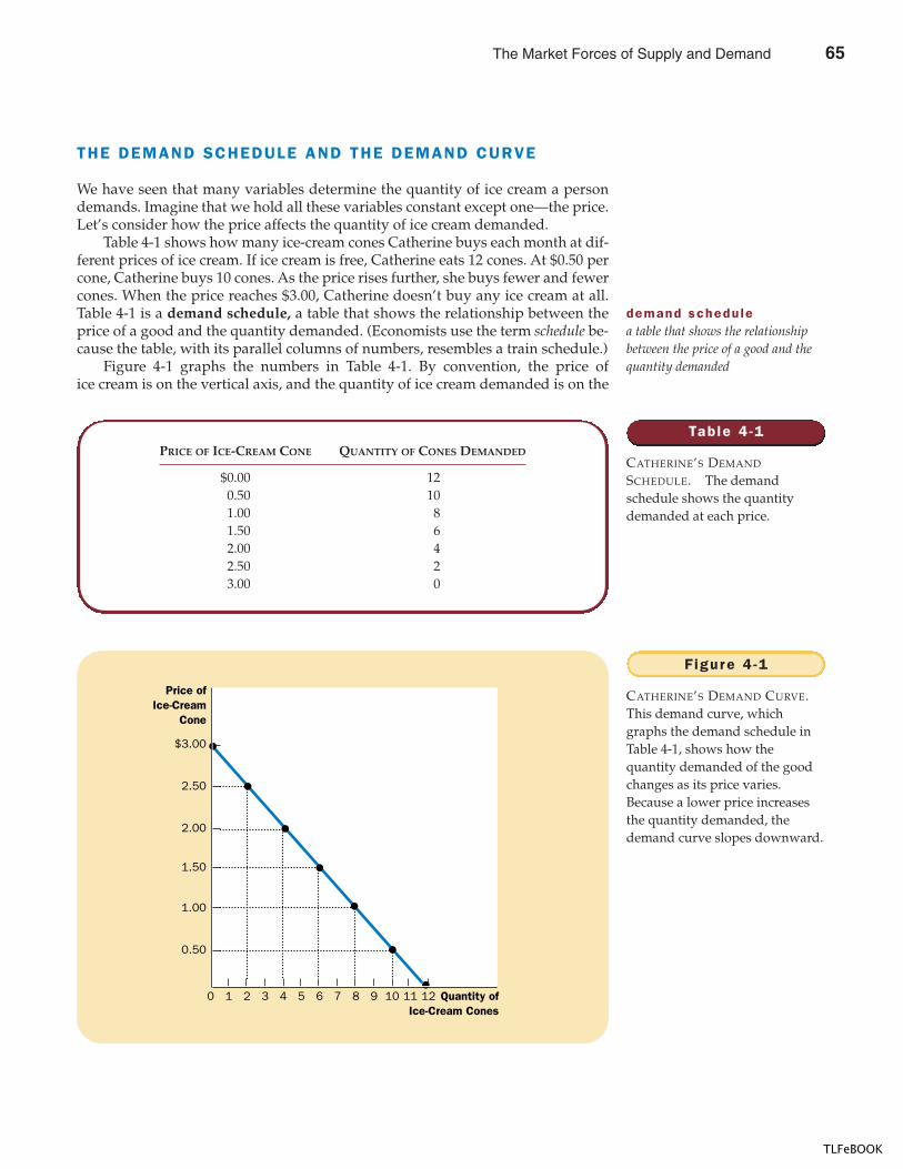
CHAPTER 4 THE MARKET FORCES OF SUPPLY AND DEMAND 69
THE DEMAND SCHEDULE AND THE DEMAND CURVE
We have seen that many variables determine the quantity of ice cream a persondemands. Imagine that we hold all these variables constant except one—the price.Let’s consider how the price affects the quantity of ice cream demanded.
Table 4-1 shows how many ice-cream cones Catherine buys each month at dif-ferent prices of ice cream. If ice cream is free, Catherine eats 12 cones. At $0.50 percone, Catherine buys 10 cones. As the price rises further, she buys fewer and fewercones. When the price reaches $3.00, Catherine doesn’t buy any ice cream at all.Table 4-1 is a demand schedule, a table that shows the relationship between theprice of a good and the quantity demanded. (Economists use the term schedule be-cause the table, with its parallel columns of numbers, resembles a train schedule.)
Figure 4-1 graphs the numbers in Table 4-1. By convention, the price ofice cream is on the vertical axis, and the quantity of ice cream demanded is on the
Table 4 -1
CATHERINE’S DEMAND
SCHEDULE. The demandschedule shows the quantitydemanded at each price.
PRICE OF ICE-CREAM CONE QUANTITY OF CONES DEMANDED
$0.00 120.50 101.00 81.50 62.00 42.50 23.00 0
demand schedu lea table that shows the relationshipbetween the price of a good and thequantity demanded
Price ofIce-Cream
Cone
0
2.50
2.00
1.50
1.00
0.50
1 2 3 4 5 6 7 8 9 10 11 Quantity ofIce-Cream Cones
$3.00
12
Figure 4 -1
CATHERINE’S DEMAND CURVE.This demand curve, whichgraphs the demand schedule inTable 4-1, shows how thequantity demanded of the goodchanges as its price varies.Because a lower price increasesthe quantity demanded, thedemand curve slopes downward.
The Market Forces of Supply and Demand 65
TLFeBOOK
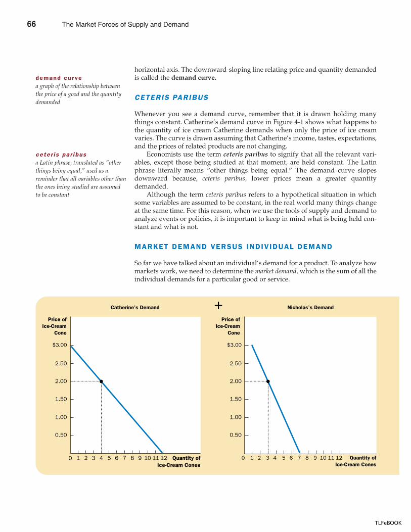
70 PART TWO SUPPLY AND DEMAND I : HOW MARKETS WORK
horizontal axis. The downward-sloping line relating price and quantity demandedis called the demand curve.
CETERIS PARIBUS
Whenever you see a demand curve, remember that it is drawn holding manythings constant. Catherine’s demand curve in Figure 4-1 shows what happens tothe quantity of ice cream Catherine demands when only the price of ice creamvaries. The curve is drawn assuming that Catherine’s income, tastes, expectations,and the prices of related products are not changing.
Economists use the term ceteris paribus to signify that all the relevant vari-ables, except those being studied at that moment, are held constant. The Latinphrase literally means “other things being equal.” The demand curve slopesdownward because, ceteris paribus, lower prices mean a greater quantitydemanded.
Although the term ceteris paribus refers to a hypothetical situation in whichsome variables are assumed to be constant, in the real world many things changeat the same time. For this reason, when we use the tools of supply and demand toanalyze events or policies, it is important to keep in mind what is being held con-stant and what is not.
MARKET DEMAND VERSUS INDIVIDUAL DEMAND
So far we have talked about an individual’s demand for a product. To analyze howmarkets work, we need to determine the market demand, which is the sum of all theindividual demands for a particular good or service.
Catherine’s Demand
Price ofIce-Cream
Cone
Price ofIce-Cream
Cone
Nicholas’s Demand
0 1 2 3 4 5 6 7 8 9 10 11 12 Quantity ofIce-Cream Cones
$3.00
1.50
2.00
2.50
1.00
0.50
0 1 2 3 4 5 6 7 8 9 10 11 12 Quantity ofIce-Cream Cones
$3.00
1.50
2.00
2.50
1.00
0.50
�
demand cur vea graph of the relationship betweenthe price of a good and the quantitydemanded
ceter is par ibusa Latin phrase, translated as “otherthings being equal,” used as areminder that all variables other thanthe ones being studied are assumedto be constant
66 The Market Forces of Supply and Demand
TLFeBOOK
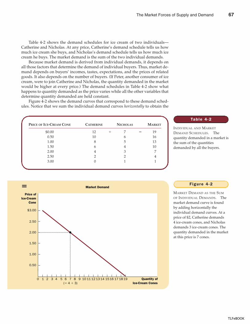
CHAPTER 4 THE MARKET FORCES OF SUPPLY AND DEMAND 71
Table 4-2 shows the demand schedules for ice cream of two individuals—Catherine and Nicholas. At any price, Catherine’s demand schedule tells us howmuch ice cream she buys, and Nicholas’s demand schedule tells us how much icecream he buys. The market demand is the sum of the two individual demands.
Because market demand is derived from individual demands, it depends onall those factors that determine the demand of individual buyers. Thus, market de-mand depends on buyers’ incomes, tastes, expectations, and the prices of relatedgoods. It also depends on the number of buyers. (If Peter, another consumer of icecream, were to join Catherine and Nicholas, the quantity demanded in the marketwould be higher at every price.) The demand schedules in Table 4-2 show whathappens to quantity demanded as the price varies while all the other variables thatdetermine quantity demanded are held constant.
Figure 4-2 shows the demand curves that correspond to these demand sched-ules. Notice that we sum the individual demand curves horizontally to obtain the
Market Demand
(� 4 � 3)
Price ofIce-Cream
Cone
0 1 2 3 4 5 6 7 8 9 10 11 12 13 14 1516 17 18 19 Quantity ofIce-Cream Cones
$3.00
1.50
2.00
2.50
1.00
0.50
� Figure 4 -2
MARKET DEMAND AS THE SUM
OF INDIVIDUAL DEMANDS. Themarket demand curve is foundby adding horizontally theindividual demand curves. At aprice of $2, Catherine demands4 ice-cream cones, and Nicholasdemands 3 ice-cream cones. Thequantity demanded in the marketat this price is 7 cones.
Table 4 -2
INDIVIDUAL AND MARKET
DEMAND SCHEDULES. Thequantity demanded in a market isthe sum of the quantitiesdemanded by all the buyers.
PRICE OF ICE-CREAM CONE CATHERINE NICHOLAS MARKET
$0.00 12 � 7 � 190.50 10 6 161.00 8 5 131.50 6 4 102.00 4 3 72.50 2 2 43.00 0 1 1
The Market Forces of Supply and Demand 67
TLFeBOOK
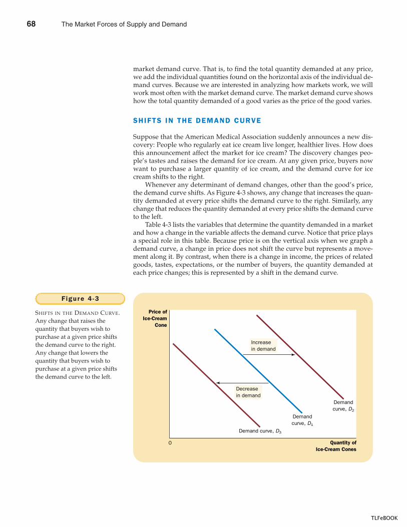
72 PART TWO SUPPLY AND DEMAND I : HOW MARKETS WORK
market demand curve. That is, to find the total quantity demanded at any price,we add the individual quantities found on the horizontal axis of the individual de-mand curves. Because we are interested in analyzing how markets work, we willwork most often with the market demand curve. The market demand curve showshow the total quantity demanded of a good varies as the price of the good varies.
SHIFTS IN THE DEMAND CURVE
Suppose that the American Medical Association suddenly announces a new dis-covery: People who regularly eat ice cream live longer, healthier lives. How doesthis announcement affect the market for ice cream? The discovery changes peo-ple’s tastes and raises the demand for ice cream. At any given price, buyers nowwant to purchase a larger quantity of ice cream, and the demand curve for icecream shifts to the right.
Whenever any determinant of demand changes, other than the good’s price,the demand curve shifts. As Figure 4-3 shows, any change that increases the quan-tity demanded at every price shifts the demand curve to the right. Similarly, anychange that reduces the quantity demanded at every price shifts the demand curveto the left.
Table 4-3 lists the variables that determine the quantity demanded in a marketand how a change in the variable affects the demand curve. Notice that price playsa special role in this table. Because price is on the vertical axis when we graph ademand curve, a change in price does not shift the curve but represents a move-ment along it. By contrast, when there is a change in income, the prices of relatedgoods, tastes, expectations, or the number of buyers, the quantity demanded ateach price changes; this is represented by a shift in the demand curve.
Price ofIce-Cream
Cone
Quantity ofIce-Cream Cones
Increasein demand
Decreasein demand
Demand curve, D3
Demandcurve, D1
Demandcurve, D2
0
Figure 4 -3
SHIFTS IN THE DEMAND CURVE.Any change that raises thequantity that buyers wish topurchase at a given price shiftsthe demand curve to the right.Any change that lowers thequantity that buyers wish topurchase at a given price shiftsthe demand curve to the left.
68 The Market Forces of Supply and Demand
TLFeBOOK
CHAPTER 4 THE MARKET FORCES OF SUPPLY AND DEMAND 73
CASE STUDY TWO WAYS TO REDUCE THE QUANTITYOF SMOKING DEMANDED
Public policymakers often want to reduce the amount that people smoke. Thereare two ways that policy can attempt to achieve this goal.
One way to reduce smoking is to shift the demand curve for cigarettes andother tobacco products. Public service announcements, mandatory health warn-ings on cigarette packages, and the prohibition of cigarette advertising on tele-vision are all policies aimed at reducing the quantity of cigarettes demanded atany given price. If successful, these policies shift the demand curve for ciga-rettes to the left, as in panel (a) of Figure 4-4.
Alternatively, policymakers can try to raise the price of cigarettes. If thegovernment taxes the manufacture of cigarettes, for example, cigarette compa-nies pass much of this tax on to consumers in the form of higher prices. A higherprice encourages smokers to reduce the numbers of cigarettes they smoke. Inthis case, the reduced amount of smoking does not represent a shift in the de-mand curve. Instead, it represents a movement along the same demand curveto a point with a higher price and lower quantity, as in panel (b) of Figure 4-4.
How much does the amount of smoking respond to changes in the price ofcigarettes? Economists have attempted to answer this question by studyingwhat happens when the tax on cigarettes changes. They have found that a10 percent increase in the price causes a 4 percent reduction in the quantity de-manded. Teenagers are found to be especially sensitive to the price of cigarettes:A 10 percent increase in the price causes a 12 percent drop in teenage smoking.
A related question is how the price of cigarettes affects the demand for illicitdrugs, such as marijuana. Opponents of cigarette taxes often argue that tobaccoand marijuana are substitutes, so that high cigarette prices encourage marijuanause. By contrast, many experts on substance abuse view tobacco as a “gatewaydrug” leading the young to experiment with other harmful substances. Moststudies of the data are consistent with this view: They find that lower cigaretteprices are associated with greater use of marijuana. In other words, tobacco andmarijuana appear to be complements rather than substitutes.
In summary, the demand curve shows what happens to the quantity demanded of agood when its price varies, holding constant all other determinants of quantity demanded.When one of these other determinants changes, the demand curve shifts.
Table 4 -3
THE DETERMINANTS OF
QUANTITY DEMANDED. Thistable lists the variables that caninfluence the quantity demandedin a market. Notice the specialrole that price plays: A change inthe price represents a movementalong the demand curve, whereasa change in one of the othervariables shifts the demandcurve.
VARIABLES THAT AFFECT
QUANTITY DEMANDED A CHANGE IN THIS VARIABLE . . .
Price Represents a movement along the demand curveIncome Shifts the demand curvePrices of related goods Shifts the demand curveTastes Shifts the demand curveExpectations Shifts the demand curveNumber of buyers Shifts the demand curve
WHAT IS THE BEST WAY TO STOP THIS?
The Market Forces of Supply and Demand 69
TLFeBOOK
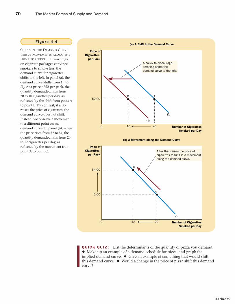
74 PART TWO SUPPLY AND DEMAND I : HOW MARKETS WORK
QUICK QUIZ: List the determinants of the quantity of pizza you demand.� Make up an example of a demand schedule for pizza, and graph theimplied demand curve. � Give an example of something that would shiftthis demand curve. � Would a change in the price of pizza shift this demandcurve?
Price ofCigarettes,
per Pack
Number of CigarettesSmoked per Day
D2
D1
0 10 20
$2.00B A
(a) A Shift in the Demand Curve
Price ofCigarettes,
per Pack
Number of CigarettesSmoked per Day
D1
0 12 20
$4.00
2.00
C
A
(b) A Movement along the Demand Curve
A tax that raises the price ofcigarettes results in a movementalong the demand curve.
A policy to discouragesmoking shifts the demand curve to the left.
Figure 4 -4
SHIFTS IN THE DEMAND CURVE
VERSUS MOVEMENTS ALONG THE
DEMAND CURVE. If warningson cigarette packages convincesmokers to smoke less, thedemand curve for cigarettesshifts to the left. In panel (a), thedemand curve shifts from D1 toD2. At a price of $2 per pack, thequantity demanded falls from20 to 10 cigarettes per day, asreflected by the shift from point Ato point B. By contrast, if a taxraises the price of cigarettes, thedemand curve does not shift.Instead, we observe a movementto a different point on thedemand curve. In panel (b), whenthe price rises from $2 to $4, thequantity demanded falls from 20to 12 cigarettes per day, asreflected by the movement frompoint A to point C.
70 The Market Forces of Supply and Demand
TLFeBOOK
CHAPTER 4 THE MARKET FORCES OF SUPPLY AND DEMAND 75
SUPPLY
We now turn to the other side of the market and examine the behavior of sellers.The quantity supplied of any good or service is the amount that sellers are willingand able to sell. Once again, to focus our thinking, let’s consider the market for icecream and look at the factors that determine the quantity supplied.
WHAT DETERMINES THE QUANTITYAN INDIVIDUAL SUPPLIES?
Imagine that you are running Student Sweets, a company that produces and sellsice cream. What determines the quantity of ice cream you are willing to produceand offer for sale? Here are some possible answers.
Pr ice The price of ice cream is one determinant of the quantity supplied. Whenthe price of ice cream is high, selling ice cream is profitable, and so the quantitysupplied is large. As a seller of ice cream, you work long hours, buy many ice-cream machines, and hire many workers. By contrast, when the price of ice creamis low, your business is less profitable, and so you will produce less ice cream. Atan even lower price, you may choose to go out of business altogether, and yourquantity supplied falls to zero.
Because the quantity supplied rises as the price rises and falls as the price falls,we say that the quantity supplied is positively related to the price of the good. Thisrelationship between price and quantity supplied is called the law of supply:Other things equal, when the price of a good rises, the quantity supplied of thegood also rises.
Input Pr ices To produce its output of ice cream, Student Sweets uses variousinputs: cream, sugar, flavoring, ice-cream machines, the buildings in which the icecream is made, and the labor of workers to mix the ingredients and operate themachines. When the price of one or more of these inputs rises, producing ice creamis less profitable, and your firm supplies less ice cream. If input prices rise sub-stantially, you might shut down your firm and supply no ice cream at all. Thus, thesupply of a good is negatively related to the price of the inputs used to make thegood.
Techno logy The technology for turning the inputs into ice cream is yet an-other determinant of supply. The invention of the mechanized ice-cream machine,for example, reduced the amount of labor necessary to make ice cream. By reduc-ing firms’ costs, the advance in technology raised the supply of ice cream.
Expectat ions The amount of ice cream you supply today may depend onyour expectations of the future. For example, if you expect the price of ice cream torise in the future, you will put some of your current production into storage andsupply less to the market today.
quant i ty supp l iedthe amount of a good that sellers arewilling and able to sell
l aw o f supp lythe claim that, other things equal, thequantity supplied of a good riseswhen the price of the good rises
The Market Forces of Supply and Demand 71
TLFeBOOK
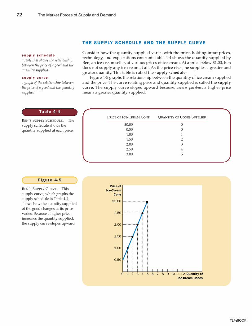
76 PART TWO SUPPLY AND DEMAND I : HOW MARKETS WORK
THE SUPPLY SCHEDULE AND THE SUPPLY CURVE
Consider how the quantity supplied varies with the price, holding input prices,technology, and expectations constant. Table 4-4 shows the quantity supplied byBen, an ice-cream seller, at various prices of ice cream. At a price below $1.00, Bendoes not supply any ice cream at all. As the price rises, he supplies a greater andgreater quantity. This table is called the supply schedule.
Figure 4-5 graphs the relationship between the quantity of ice cream suppliedand the price. The curve relating price and quantity supplied is called the supplycurve. The supply curve slopes upward because, ceteris paribus, a higher pricemeans a greater quantity supplied.
Table 4 -4
BEN’S SUPPLY SCHEDULE. Thesupply schedule shows thequantity supplied at each price.
PRICE OF ICE-CREAM CONE QUANTITY OF CONES SUPPLIED
$0.00 00.50 01.00 11.50 22.00 32.50 43.00 5
supp ly schedu lea table that shows the relationshipbetween the price of a good and thequantity supplied
supp ly cur vea graph of the relationship betweenthe price of a good and the quantitysupplied
Price ofIce-Cream
Cone
0
2.50
2.00
1.50
1.00
1 2 3 4 5 6 7 8 9 10 11 Quantity ofIce-Cream Cones
$3.00
12
0.50
Figure 4 -5
BEN’S SUPPLY CURVE. Thissupply curve, which graphs thesupply schedule in Table 4-4,shows how the quantity suppliedof the good changes as its pricevaries. Because a higher priceincreases the quantity supplied,the supply curve slopes upward.
72 The Market Forces of Supply and Demand
TLFeBOOK
CHAPTER 4 THE MARKET FORCES OF SUPPLY AND DEMAND 77
MARKET SUPPLY VERSUS INDIVIDUAL SUPPLY
Just as market demand is the sum of the demands of all buyers, market supply isthe sum of the supplies of all sellers. Table 4-5 shows the supply schedules for twoice-cream producers—Ben and Jerry. At any price, Ben’s supply schedule tells usthe quantity of ice cream Ben supplies, and Jerry’s supply schedule tells us thequantity of ice cream Jerry supplies. The market supply is the sum of the two in-dividual supplies.
Market supply depends on all those factors that influence the supply of indi-vidual sellers, such as the prices of inputs used to produce the good, the availabletechnology, and expectations. In addition, the supply in a market depends on thenumber of sellers. (If Ben or Jerry were to retire from the ice-cream business, thesupply in the market would fall.) The supply schedules in Table 4-5 show whathappens to quantity supplied as the price varies while all the other variables thatdetermine quantity supplied are held constant.
Figure 4-6 shows the supply curves that correspond to the supply schedules inTable 4-5. As with demand curves, we sum the individual supply curves horizon-tally to obtain the market supply curve. That is, to find the total quantity suppliedat any price, we add the individual quantities found on the horizontal axis of theindividual supply curves. The market supply curve shows how the total quantitysupplied varies as the price of the good varies.
SHIFTS IN THE SUPPLY CURVE
Suppose that the price of sugar falls. How does this change affect the supply of icecream? Because sugar is an input into producing ice cream, the fall in the price ofsugar makes selling ice cream more profitable. This raises the supply of ice cream:At any given price, sellers are now willing to produce a larger quantity. Thus, thesupply curve for ice cream shifts to the right.
Whenever there is a change in any determinant of supply, other than thegood’s price, the supply curve shifts. As Figure 4-7 shows, any change that raisesquantity supplied at every price shifts the supply curve to the right. Similarly, anychange that reduces the quantity supplied at every price shifts the supply curve tothe left.
Table 4 -5
INDIVIDUAL AND MARKET
SUPPLY SCHEDULES. Thequantity supplied in a market isthe sum of the quantitiessupplied by all the sellers.
PRICE OF ICE-CREAM CONE BEN JERRY MARKET
$0.00 0 � 0 � 00.50 0 0 01.00 1 0 11.50 2 2 42.00 3 4 72.50 4 6 103.00 5 8 13
The Market Forces of Supply and Demand 73
TLFeBOOK
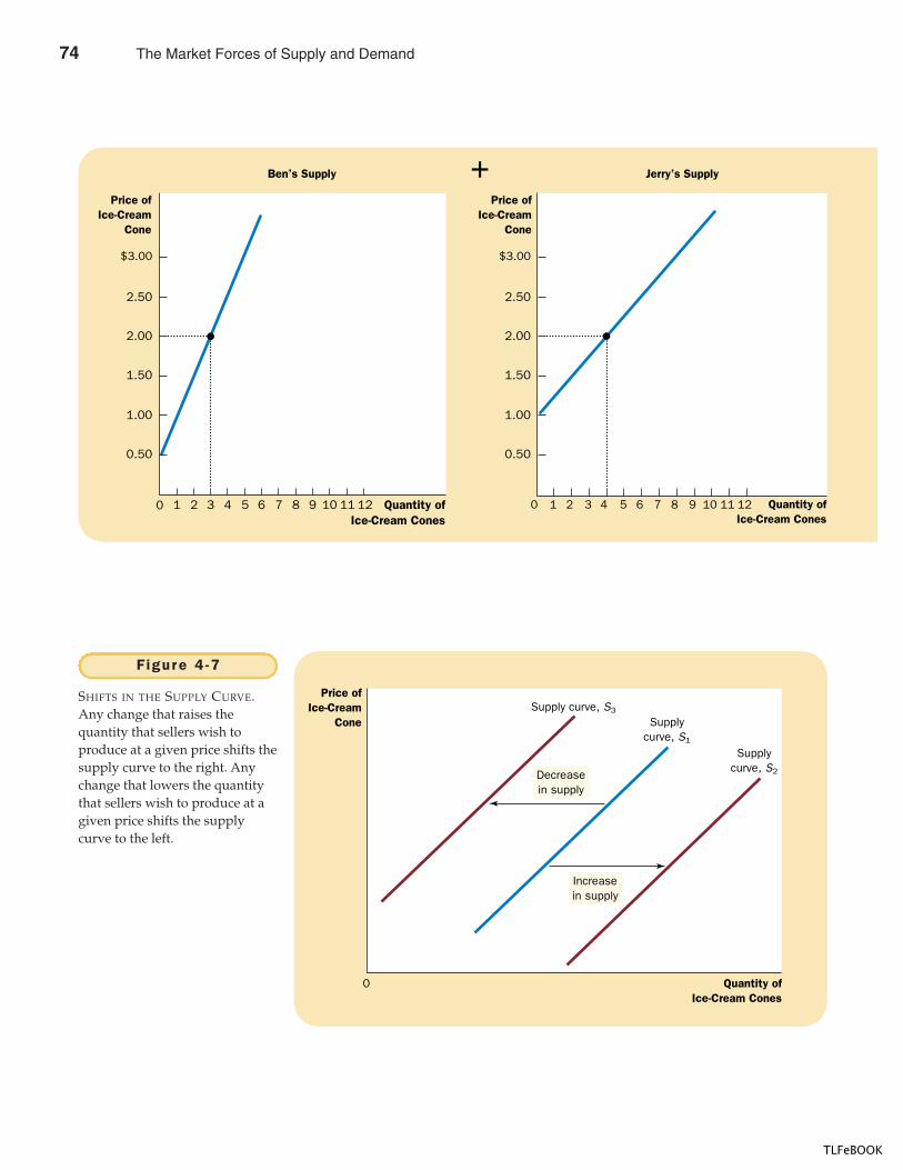
78 PART TWO SUPPLY AND DEMAND I : HOW MARKETS WORK
Ben’s Supply
Price ofIce-Cream
Cone
Price ofIce-Cream
Cone
� Jerry’s Supply
0 1 2 3 4 5 6 7 8 9 10 11 12 Quantity ofIce-Cream Cones
$3.00
1.50
2.00
2.50
1.00
0.50
0 1 2 3 4 5 6 7 8 9 10 11 12 Quantity ofIce-Cream Cones
$3.00
1.50
2.00
2.50
1.00
0.50
Price ofIce-Cream
Cone
Quantity ofIce-Cream Cones
0
Increasein supply
Decreasein supply
Supply curve, S3
Supplycurve, S1
Supplycurve, S2
Figure 4 -7
SHIFTS IN THE SUPPLY CURVE.Any change that raises thequantity that sellers wish toproduce at a given price shifts thesupply curve to the right. Anychange that lowers the quantitythat sellers wish to produce at agiven price shifts the supplycurve to the left.
74 The Market Forces of Supply and Demand
TLFeBOOK
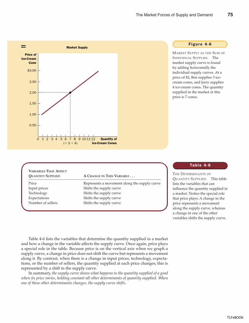
CHAPTER 4 THE MARKET FORCES OF SUPPLY AND DEMAND 79
Table 4-6 lists the variables that determine the quantity supplied in a marketand how a change in the variable affects the supply curve. Once again, price playsa special role in the table. Because price is on the vertical axis when we graph asupply curve, a change in price does not shift the curve but represents a movementalong it. By contrast, when there is a change in input prices, technology, expecta-tions, or the number of sellers, the quantity supplied at each price changes; this isrepresented by a shift in the supply curve.
In summary, the supply curve shows what happens to the quantity supplied of a goodwhen its price varies, holding constant all other determinants of quantity supplied. Whenone of these other determinants changes, the supply curve shifts.
Market Supply
(� 3 � 4)
Price ofIce-Cream
Cone
0 1 2 3 4 5 6 7 8 9 10 11 12 Quantity ofIce-Cream Cones
$3.00
1.50
2.00
2.50
1.00
0.50
� Figure 4 -6
MARKET SUPPLY AS THE SUM OF
INDIVIDUAL SUPPLIES. Themarket supply curve is foundby adding horizontally theindividual supply curves. At aprice of $2, Ben supplies 3 ice-cream cones, and Jerry supplies4 ice-cream cones. The quantitysupplied in the market at thisprice is 7 cones.
Table 4 -6
THE DETERMINANTS OF
QUANTITY SUPPLIED. This tablelists the variables that caninfluence the quantity supplied ina market. Notice the special rolethat price plays: A change in theprice represents a movementalong the supply curve, whereasa change in one of the othervariables shifts the supply curve.
VARIABLES THAT AFFECT
QUANTITY SUPPLIED A CHANGE IN THIS VARIABLE . . .
Price Represents a movement along the supply curveInput prices Shifts the supply curveTechnology Shifts the supply curveExpectations Shifts the supply curveNumber of sellers Shifts the supply curve
The Market Forces of Supply and Demand 75
TLFeBOOK
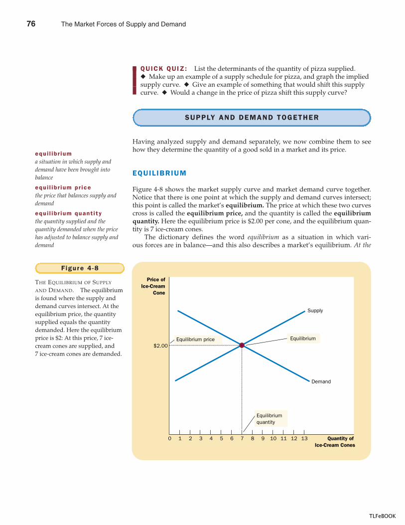
80 PART TWO SUPPLY AND DEMAND I : HOW MARKETS WORK
QUICK QUIZ: List the determinants of the quantity of pizza supplied.� Make up an example of a supply schedule for pizza, and graph the implied supply curve. � Give an example of something that would shift this supply curve. � Would a change in the price of pizza shift this supply curve?
SUPPLY AND DEMAND TOGETHER
Having analyzed supply and demand separately, we now combine them to seehow they determine the quantity of a good sold in a market and its price.
EQUIL IBRIUM
Figure 4-8 shows the market supply curve and market demand curve together.Notice that there is one point at which the supply and demand curves intersect;this point is called the market’s equilibrium. The price at which these two curvescross is called the equilibrium price, and the quantity is called the equilibriumquantity. Here the equilibrium price is $2.00 per cone, and the equilibrium quan-tity is 7 ice-cream cones.
The dictionary defines the word equilibrium as a situation in which vari-ous forces are in balance—and this also describes a market’s equilibrium. At the
equi l ib r iuma situation in which supply and demand have been brought intobalance
equi l ib r ium pr icethe price that balances supply anddemand
equi l ib r ium quant i tythe quantity supplied and thequantity demanded when the pricehas adjusted to balance supply anddemand
Price ofIce-Cream
Cone
$2.00
0 1 2 3 4 5 6 7 8 9 10 11 12 Quantity of Ice-Cream Cones
13
Equilibriumquantity
Equilibrium price Equilibrium
Supply
Demand
Figure 4 -8
THE EQUILIBRIUM OF SUPPLY
AND DEMAND. The equilibriumis found where the supply anddemand curves intersect. At theequilibrium price, the quantitysupplied equals the quantitydemanded. Here the equilibriumprice is $2: At this price, 7 ice-cream cones are supplied, and7 ice-cream cones are demanded.
76 The Market Forces of Supply and Demand
TLFeBOOK
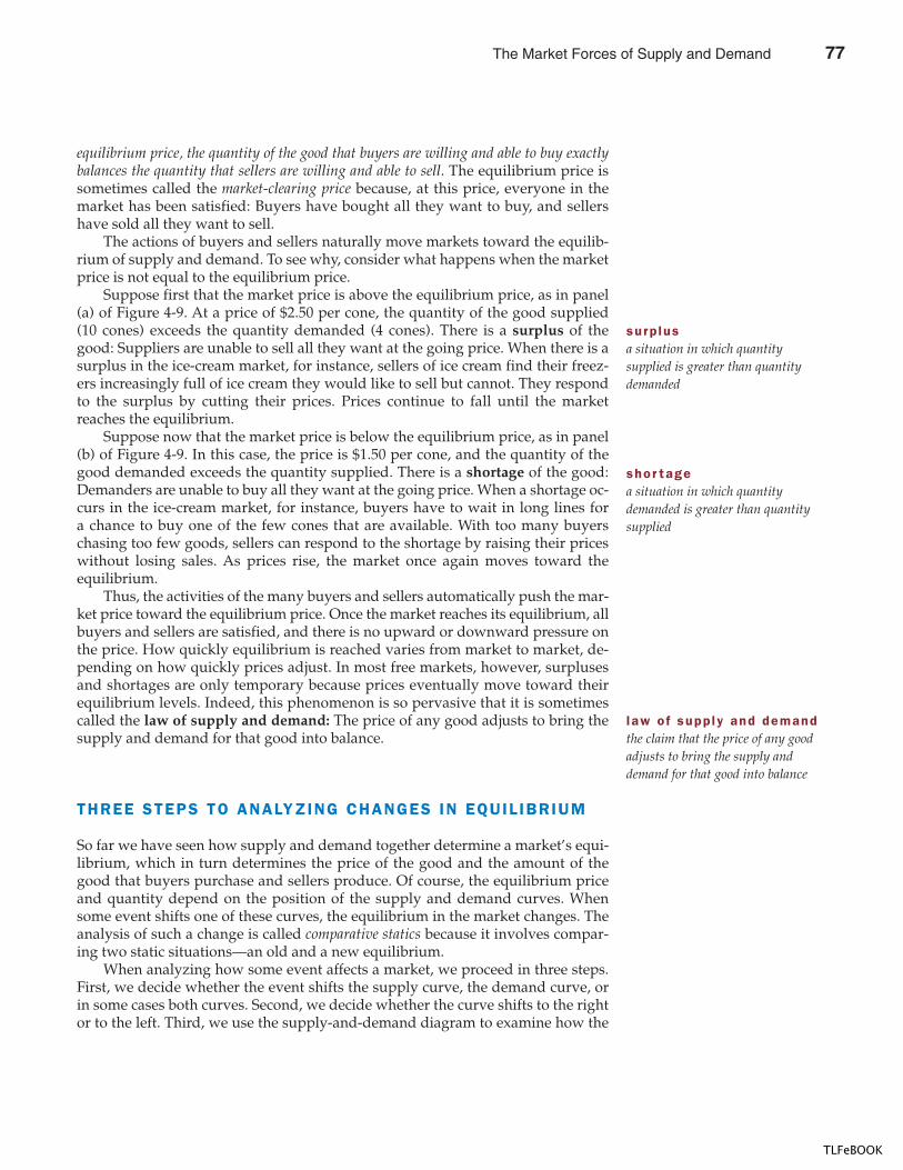
CHAPTER 4 THE MARKET FORCES OF SUPPLY AND DEMAND 81
equilibrium price, the quantity of the good that buyers are willing and able to buy exactlybalances the quantity that sellers are willing and able to sell. The equilibrium price issometimes called the market-clearing price because, at this price, everyone in themarket has been satisfied: Buyers have bought all they want to buy, and sellershave sold all they want to sell.
The actions of buyers and sellers naturally move markets toward the equilib-rium of supply and demand. To see why, consider what happens when the marketprice is not equal to the equilibrium price.
Suppose first that the market price is above the equilibrium price, as in panel(a) of Figure 4-9. At a price of $2.50 per cone, the quantity of the good supplied(10 cones) exceeds the quantity demanded (4 cones). There is a surplus of thegood: Suppliers are unable to sell all they want at the going price. When there is asurplus in the ice-cream market, for instance, sellers of ice cream find their freez-ers increasingly full of ice cream they would like to sell but cannot. They respondto the surplus by cutting their prices. Prices continue to fall until the marketreaches the equilibrium.
Suppose now that the market price is below the equilibrium price, as in panel(b) of Figure 4-9. In this case, the price is $1.50 per cone, and the quantity of thegood demanded exceeds the quantity supplied. There is a shortage of the good:Demanders are unable to buy all they want at the going price. When a shortage oc-curs in the ice-cream market, for instance, buyers have to wait in long lines fora chance to buy one of the few cones that are available. With too many buyerschasing too few goods, sellers can respond to the shortage by raising their priceswithout losing sales. As prices rise, the market once again moves toward theequilibrium.
Thus, the activities of the many buyers and sellers automatically push the mar-ket price toward the equilibrium price. Once the market reaches its equilibrium, allbuyers and sellers are satisfied, and there is no upward or downward pressure onthe price. How quickly equilibrium is reached varies from market to market, de-pending on how quickly prices adjust. In most free markets, however, surplusesand shortages are only temporary because prices eventually move toward theirequilibrium levels. Indeed, this phenomenon is so pervasive that it is sometimescalled the law of supply and demand: The price of any good adjusts to bring thesupply and demand for that good into balance.
THREE STEPS TO ANALYZING CHANGES IN EQUIL IBRIUM
So far we have seen how supply and demand together determine a market’s equi-librium, which in turn determines the price of the good and the amount of thegood that buyers purchase and sellers produce. Of course, the equilibrium priceand quantity depend on the position of the supply and demand curves. Whensome event shifts one of these curves, the equilibrium in the market changes. Theanalysis of such a change is called comparative statics because it involves compar-ing two static situations—an old and a new equilibrium.
When analyzing how some event affects a market, we proceed in three steps.First, we decide whether the event shifts the supply curve, the demand curve, orin some cases both curves. Second, we decide whether the curve shifts to the rightor to the left. Third, we use the supply-and-demand diagram to examine how the
surp lusa situation in which quantitysupplied is greater than quantitydemanded
shor tagea situation in which quantitydemanded is greater than quantitysupplied
l aw o f supp ly and demandthe claim that the price of any goodadjusts to bring the supply anddemand for that good into balance
The Market Forces of Supply and Demand 77
TLFeBOOK
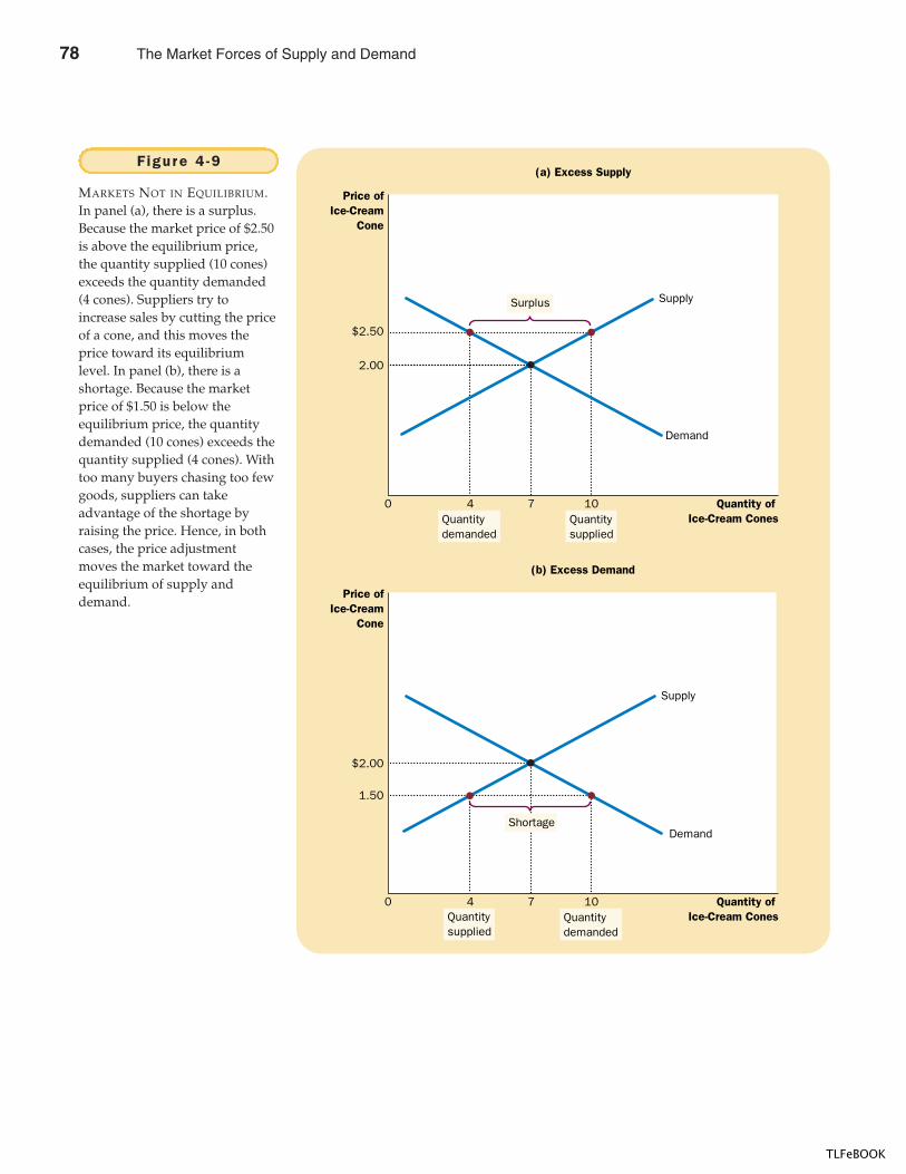
82 PART TWO SUPPLY AND DEMAND I : HOW MARKETS WORK
Price ofIce-Cream
Cone
2.00
$2.50
0 4 7 10 Quantity of Ice-Cream Cones
Supply
Demand
(a) Excess Supply
Quantitydemanded
Quantitysupplied
Surplus
Price ofIce-Cream
Cone
$2.00
1.50
0 4 7 10 Quantity of Ice-Cream Cones
Supply
Demand
(b) Excess Demand
Quantitysupplied
Quantitydemanded
Shortage
Figure 4 -9
MARKETS NOT IN EQUILIBRIUM.In panel (a), there is a surplus.Because the market price of $2.50is above the equilibrium price,the quantity supplied (10 cones)exceeds the quantity demanded(4 cones). Suppliers try toincrease sales by cutting the priceof a cone, and this moves theprice toward its equilibriumlevel. In panel (b), there is ashortage. Because the marketprice of $1.50 is below theequilibrium price, the quantitydemanded (10 cones) exceeds thequantity supplied (4 cones). Withtoo many buyers chasing too fewgoods, suppliers can takeadvantage of the shortage byraising the price. Hence, in bothcases, the price adjustmentmoves the market toward theequilibrium of supply anddemand.
78 The Market Forces of Supply and Demand
TLFeBOOK
CHAPTER 4 THE MARKET FORCES OF SUPPLY AND DEMAND 83
shift affects the equilibrium price and quantity. Table 4-7 summarizes these threesteps. To see how this recipe is used, let’s consider various events that might affectthe market for ice cream.
Example: A Change in Demand Suppose that one summer the weatheris very hot. How does this event affect the market for ice cream? To answer thisquestion, let’s follow our three steps.
1. The hot weather affects the demand curve by changing people’s taste for icecream. That is, the weather changes the amount of ice cream that peoplewant to buy at any given price. The supply curve is unchanged because theweather does not directly affect the firms that sell ice cream.
2. Because hot weather makes people want to eat more ice cream, the demandcurve shifts to the right. Figure 4-10 shows this increase in demand as theshift in the demand curve from D1 to D2. This shift indicates that the quantityof ice cream demanded is higher at every price.
3. As Figure 4-10 shows, the increase in demand raises the equilibrium pricefrom $2.00 to $2.50 and the equilibrium quantity from 7 to 10 cones. In otherwords, the hot weather increases the price of ice cream and the quantity ofice cream sold.
Shifts in Curves versus Movements along Curves Notice that whenhot weather drives up the price of ice cream, the quantity of ice cream that firms sup-ply rises, even though the supply curve remains the same. In this case, economistssay there has been an increase in “quantity supplied” but no change in “supply.”
Table 4 -7
A THREE-STEP PROGRAM FOR
ANALYZING CHANGES IN
EQUILIBRIUM
1. Decide whether the event shifts the supply curve or demand curve (or perhapsboth).
2. Decide which direction the curve shifts.3. Use the supply-and-demand diagram to see how the shift changes the
equilibrium.
The Market Forces of Supply and Demand 79
TLFeBOOK
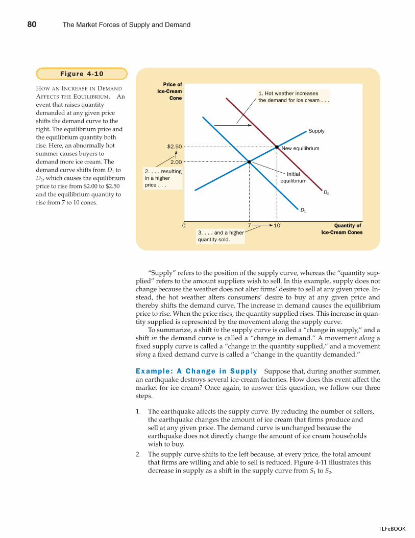
84 PART TWO SUPPLY AND DEMAND I : HOW MARKETS WORK
“Supply” refers to the position of the supply curve, whereas the “quantity sup-plied” refers to the amount suppliers wish to sell. In this example, supply does notchange because the weather does not alter firms’ desire to sell at any given price. In-stead, the hot weather alters consumers’ desire to buy at any given price andthereby shifts the demand curve. The increase in demand causes the equilibriumprice to rise. When the price rises, the quantity supplied rises. This increase in quan-tity supplied is represented by the movement along the supply curve.
To summarize, a shift in the supply curve is called a “change in supply,” and ashift in the demand curve is called a “change in demand.” A movement along afixed supply curve is called a “change in the quantity supplied,” and a movementalong a fixed demand curve is called a “change in the quantity demanded.”
Example : A Change in Supp ly Suppose that, during another summer,an earthquake destroys several ice-cream factories. How does this event affect themarket for ice cream? Once again, to answer this question, we follow our threesteps.
1. The earthquake affects the supply curve. By reducing the number of sellers,the earthquake changes the amount of ice cream that firms produce and sell at any given price. The demand curve is unchanged because theearthquake does not directly change the amount of ice cream householdswish to buy.
2. The supply curve shifts to the left because, at every price, the total amountthat firms are willing and able to sell is reduced. Figure 4-11 illustrates thisdecrease in supply as a shift in the supply curve from S1 to S2.
Price ofIce-Cream
Cone
2.00
$2.50
0 7 10 Quantity of Ice-Cream Cones
Supply
New equilibrium
Initialequilibrium
D1
D2
3. . . . and a higherquantity sold.
2. . . . resultingin a higherprice . . .
1. Hot weather increasesthe demand for ice cream . . .
Figure 4 -10
HOW AN INCREASE IN DEMAND
AFFECTS THE EQUILIBRIUM. Anevent that raises quantitydemanded at any given priceshifts the demand curve to theright. The equilibrium price andthe equilibrium quantity bothrise. Here, an abnormally hotsummer causes buyers todemand more ice cream. Thedemand curve shifts from D1 toD2, which causes the equilibriumprice to rise from $2.00 to $2.50and the equilibrium quantity torise from 7 to 10 cones.
80 The Market Forces of Supply and Demand
TLFeBOOK
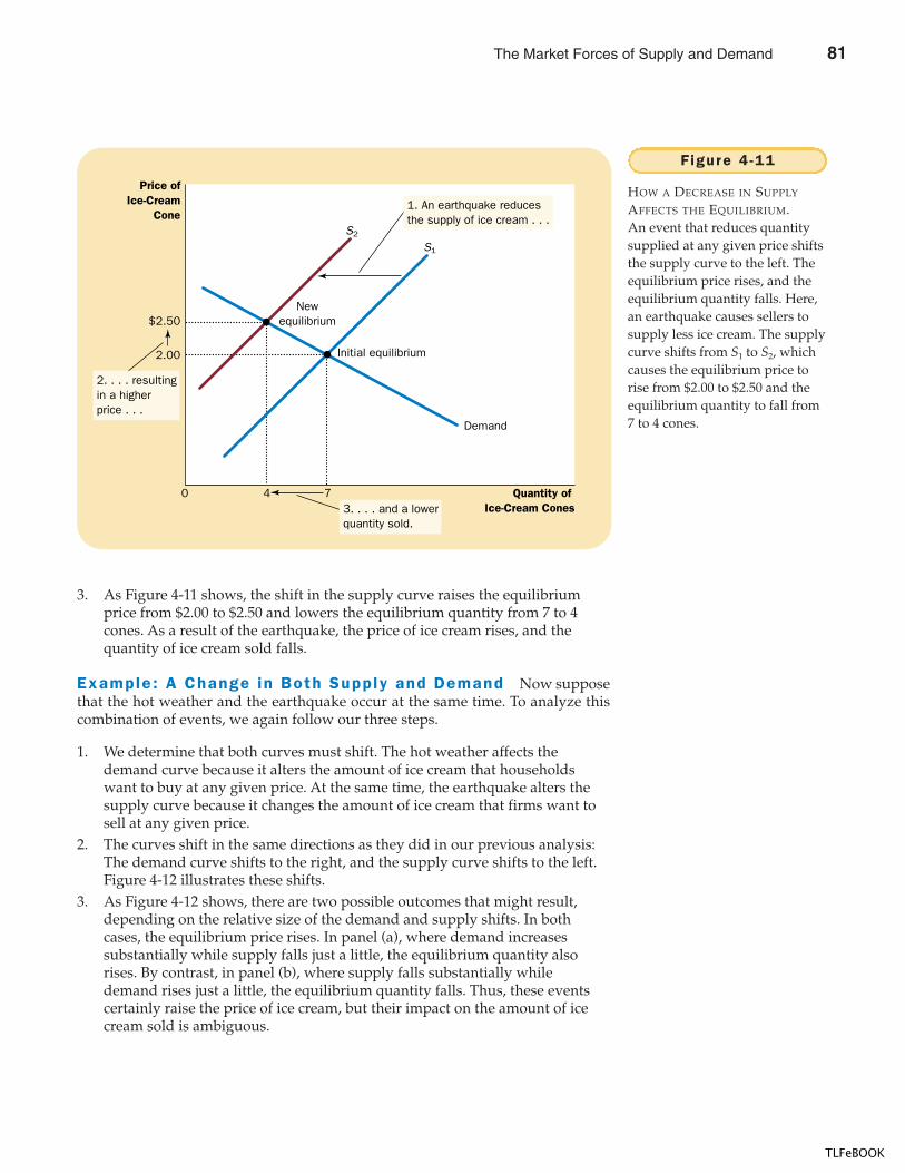
CHAPTER 4 THE MARKET FORCES OF SUPPLY AND DEMAND 85
3. As Figure 4-11 shows, the shift in the supply curve raises the equilibriumprice from $2.00 to $2.50 and lowers the equilibrium quantity from 7 to 4cones. As a result of the earthquake, the price of ice cream rises, and thequantity of ice cream sold falls.
Example : A Change in Both Supply and Demand Now supposethat the hot weather and the earthquake occur at the same time. To analyze thiscombination of events, we again follow our three steps.
1. We determine that both curves must shift. The hot weather affects thedemand curve because it alters the amount of ice cream that householdswant to buy at any given price. At the same time, the earthquake alters thesupply curve because it changes the amount of ice cream that firms want tosell at any given price.
2. The curves shift in the same directions as they did in our previous analysis:The demand curve shifts to the right, and the supply curve shifts to the left.Figure 4-12 illustrates these shifts.
3. As Figure 4-12 shows, there are two possible outcomes that might result,depending on the relative size of the demand and supply shifts. In bothcases, the equilibrium price rises. In panel (a), where demand increasessubstantially while supply falls just a little, the equilibrium quantity alsorises. By contrast, in panel (b), where supply falls substantially whiledemand rises just a little, the equilibrium quantity falls. Thus, these eventscertainly raise the price of ice cream, but their impact on the amount of icecream sold is ambiguous.
Price ofIce-Cream
Cone
2.00
$2.50
0 4 7 Quantity of Ice-Cream Cones
Demand
Newequilibrium
Initial equilibrium
S1
S2
2. . . . resultingin a higherprice . . .
1. An earthquake reducesthe supply of ice cream . . .
3. . . . and a lowerquantity sold.
Figure 4 -11
HOW A DECREASE IN SUPPLY
AFFECTS THE EQUILIBRIUM.An event that reduces quantitysupplied at any given price shiftsthe supply curve to the left. Theequilibrium price rises, and theequilibrium quantity falls. Here,an earthquake causes sellers tosupply less ice cream. The supplycurve shifts from S1 to S2, whichcauses the equilibrium price torise from $2.00 to $2.50 and theequilibrium quantity to fall from7 to 4 cones.
The Market Forces of Supply and Demand 81
TLFeBOOK
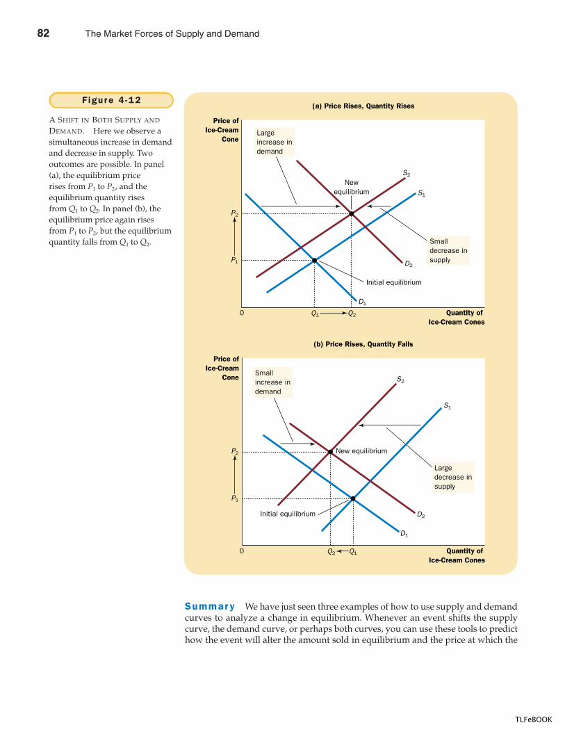
86 PART TWO SUPPLY AND DEMAND I : HOW MARKETS WORK
Summar y We have just seen three examples of how to use supply and demandcurves to analyze a change in equilibrium. Whenever an event shifts the supplycurve, the demand curve, or perhaps both curves, you can use these tools to predicthow the event will alter the amount sold in equilibrium and the price at which the
(b) Price Rises, Quantity Falls
Price ofIce-Cream
Cone
Quantity of Ice-Cream Cones
0
New equilibrium
Initial equilibrium
S1
D1
D2
S2
Q1Q2
P2
P1
(a) Price Rises, Quantity Rises
Price ofIce-Cream
Cone
Quantity of Ice-Cream Cones
0
Newequilibrium
Initial equilibrium
S1
D1
D2
S2
Q1 Q2
P2
P1
Largeincrease indemand
Smalldecrease insupply
Smallincrease indemand
Largedecrease insupply
Figure 4 -12
A SHIFT IN BOTH SUPPLY AND
DEMAND. Here we observe asimultaneous increase in demandand decrease in supply. Twooutcomes are possible. In panel(a), the equilibrium pricerises from P1 to P2, and theequilibrium quantity risesfrom Q1 to Q2. In panel (b), theequilibrium price again risesfrom P1 to P2, but the equilibriumquantity falls from Q1 to Q2.
82 The Market Forces of Supply and Demand
TLFeBOOK
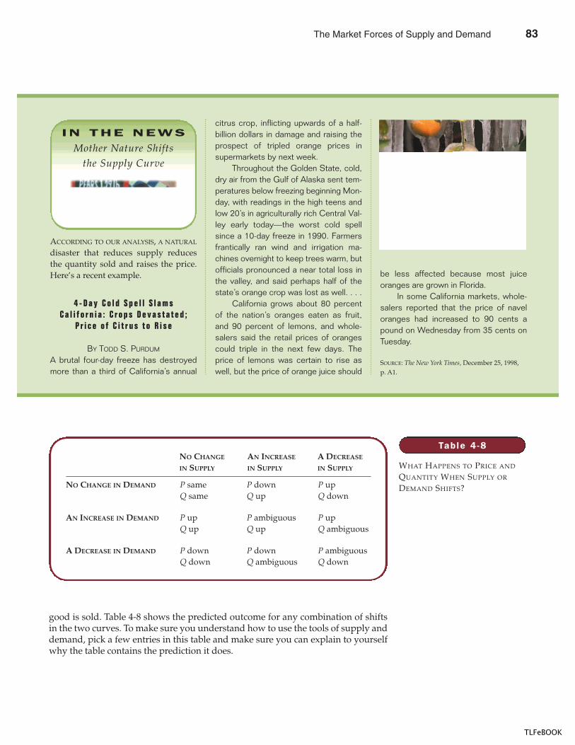
CHAPTER 4 THE MARKET FORCES OF SUPPLY AND DEMAND 87
good is sold. Table 4-8 shows the predicted outcome for any combination of shiftsin the two curves. To make sure you understand how to use the tools of supply anddemand, pick a few entries in this table and make sure you can explain to yourselfwhy the table contains the prediction it does.
ACCORDING TO OUR ANALYSIS, A NATURAL
disaster that reduces supply reducesthe quantity sold and raises the price.Here’s a recent example.
4 - D a y C o l d S p e l l S l a m sC a l i f o r n i a : C r o p s D e v a s t a t e d ;
P r i c e o f C i t r u s t o R i s e
BY TODD S. PURDUM
A brutal four-day freeze has destroyedmore than a third of California’s annual
citrus crop, inflicting upwards of a half-billion dollars in damage and raising theprospect of tripled orange prices insupermarkets by next week.
Throughout the Golden State, cold,dry air from the Gulf of Alaska sent tem-peratures below freezing beginning Mon-day, with readings in the high teens andlow 20’s in agriculturally rich Central Val-ley early today—the worst cold spellsince a 10-day freeze in 1990. Farmersfrantically ran wind and irrigation ma-chines overnight to keep trees warm, butofficials pronounced a near total loss inthe valley, and said perhaps half of thestate’s orange crop was lost as well. . . .
California grows about 80 percentof the nation’s oranges eaten as fruit,and 90 percent of lemons, and whole-salers said the retail prices of orangescould triple in the next few days. Theprice of lemons was certain to rise aswell, but the price of orange juice should
be less affected because most juiceoranges are grown in Florida.
In some California markets, whole-salers reported that the price of naveloranges had increased to 90 cents apound on Wednesday from 35 cents onTuesday.
SOURCE: The New York Times, December 25, 1998,p. A1.
IN THE NEWS
Mother Nature Shiftsthe Supply Curve
Table 4 -8
WHAT HAPPENS TO PRICE AND
QUANTITY WHEN SUPPLY OR
DEMAND SHIFTS?
NO CHANGE AN INCREASE A DECREASE
IN SUPPLY IN SUPPLY IN SUPPLY
NO CHANGE IN DEMAND P same P down P upQ same Q up Q down
AN INCREASE IN DEMAND P up P ambiguous P upQ up Q up Q ambiguous
A DECREASE IN DEMAND P down P down P ambiguousQ down Q ambiguous Q down
The Market Forces of Supply and Demand 83
TLFeBOOK
88 PART TWO SUPPLY AND DEMAND I : HOW MARKETS WORK
QUICK QUIZ: Analyze what happens to the market for pizza if the price oftomatoes rises. � Analyze what happens to the market for pizza if the price of hamburgers falls.
CONCLUSION: HOW PRICES ALLOCATE RESOURCES
This chapter has analyzed supply and demand in a single market. Although ourdiscussion has centered around the market for ice cream, the lessons learned hereapply in most other markets as well. Whenever you go to a store to buy something,you are contributing to the demand for that item. Whenever you look for a job,you are contributing to the supply of labor services. Because supply and demandare such pervasive economic phenomena, the model of supply and demand is apowerful tool for analysis. We will be using this model repeatedly in the followingchapters.
One of the Ten Principles of Economics discussed in Chapter 1 is that markets areusually a good way to organize economic activity. Although it is still too early tojudge whether market outcomes are good or bad, in this chapter we have begun tosee how markets work. In any economic system, scarce resources have to be allo-cated among competing uses. Market economies harness the forces of supply anddemand to serve that end. Supply and demand together determine the prices ofthe economy’s many different goods and services; prices in turn are the signalsthat guide the allocation of resources.
For example, consider the allocation of beachfront land. Because the amountof this land is limited, not everyone can enjoy the luxury of living by the beach.Who gets this resource? The answer is: whoever is willing and able to pay theprice. The price of beachfront land adjusts until the quantity of land demanded ex-actly balances the quantity supplied. Thus, in market economies, prices are themechanism for rationing scarce resources.
Similarly, prices determine who produces each good and how much is pro-duced. For instance, consider farming. Because we need food to survive, it is cru-cial that some people work on farms. What determines who is a farmer and who isnot? In a free society, there is no government planning agency making this decisionand ensuring an adequate supply of food. Instead, the allocation of workers tofarms is based on the job decisions of millions of workers. This decentralized sys-tem works well because these decisions depend on prices. The prices of food andthe wages of farmworkers (the price of their labor) adjust to ensure that enoughpeople choose to be farmers.
If a person had never seen a market economy in action, the whole idea mightseem preposterous. Economies are large groups of people engaged in many inter-dependent activities. What prevents decentralized decisionmaking from degen-erating into chaos? What coordinates the actions of the millions of people withtheir varying abilities and desires? What ensures that what needs to get donedoes in fact get done? The answer, in a word, is prices. If market economiesare guided by an invisible hand, as Adam Smith famously suggested, then theprice system is the baton that the invisible hand uses to conduct the economicorchestra.
84 The Market Forces of Supply and Demand
TLFeBOOK
CHAPTER 4 THE MARKET FORCES OF SUPPLY AND DEMAND 89
“—and seventy-five cents.”“Two dollars.”
� Economists use the model of supply and demand to analyze competitive markets. In a competitivemarket, there are many buyers and sellers, each of whom has little or no influence on the market price.
� The demand curve shows how the quantity of a gooddemanded depends on the price. According to the lawof demand, as the price of a good falls, the quantitydemanded rises. Therefore, the demand curve slopesdownward.
� In addition to price, other determinants of the quantitydemanded include income, tastes, expectations, and the prices of substitutes and complements. If one ofthese other determinants changes, the demand curveshifts.
� The supply curve shows how the quantity of a goodsupplied depends on the price. According to the law ofsupply, as the price of a good rises, the quantitysupplied rises. Therefore, the supply curve slopesupward.
� In addition to price, other determinants of the quantitysupplied include input prices, technology, andexpectations. If one of these other determinants changes,the supply curve shifts.
� The intersection of the supply and demand curvesdetermines the market equilibrium. At the equilibrium
price, the quantity demanded equals the quantitysupplied.
� The behavior of buyers and sellers naturally drivesmarkets toward their equilibrium. When the marketprice is above the equilibrium price, there is a surplus of the good, which causes the market price to fall. When the market price is below the equilibriumprice, there is a shortage, which causes the market priceto rise.
� To analyze how any event influences a market, we usethe supply-and-demand diagram to examine how theevent affects the equilibrium price and quantity. To dothis we follow three steps. First, we decide whether theevent shifts the supply curve or the demand curve (orboth). Second, we decide which direction the curveshifts. Third, we compare the new equilibrium with theold equilibrium.
� In market economies, prices are the signals that guideeconomic decisions and thereby allocate scarceresources. For every good in the economy, the priceensures that supply and demand are in balance. Theequilibrium price then determines how much of thegood buyers choose to purchase and how much sellerschoose to produce.
Summar y
The Market Forces of Supply and Demand 85
TLFeBOOK
90 PART TWO SUPPLY AND DEMAND I : HOW MARKETS WORK
market, p. 66competitive market, p. 66quantity demanded, p. 67law of demand, p. 68normal good, p. 68inferior good, p. 68substitutes, p. 68
complements, p. 68demand schedule, p. 69demand curve, p. 70ceteris paribus, p. 70quantity supplied, p. 75law of supply, p. 75supply schedule, p. 76
supply curve, p. 76equilibrium, p. 80equilibrium price, p. 80equilibrium quantity, p. 80surplus, p. 81shortage, p. 81law of supply and demand, p. 81
Key Concepts
1. What is a competitive market? Briefly describe the types of markets other than perfectly competitivemarkets.
2. What determines the quantity of a good that buyersdemand?
3. What are the demand schedule and the demand curve,and how are they related? Why does the demand curveslope downward?
4. Does a change in consumers’ tastes lead to a movementalong the demand curve or a shift in the demand curve?Does a change in price lead to a movement along thedemand curve or a shift in the demand curve?
5. Popeye’s income declines and, as a result, he buys more spinach. Is spinach an inferior or a normal good? What happens to Popeye’s demand curve forspinach?
6. What determines the quantity of a good that sellerssupply?
7. What are the supply schedule and the supply curve, andhow are they related? Why does the supply curve slopeupward?
8. Does a change in producers’ technology lead to amovement along the supply curve or a shift in thesupply curve? Does a change in price lead to amovement along the supply curve or a shift in thesupply curve?
9. Define the equilibrium of a market. Describe the forcesthat move a market toward its equilibrium.
10. Beer and pizza are complements because they are oftenenjoyed together. When the price of beer rises, whathappens to the supply, demand, quantity supplied,quantity demanded, and the price in the market forpizza?
11. Describe the role of prices in market economies.
Quest ions fo r Rev iew
1. Explain each of the following statements using supply-and-demand diagrams.a. When a cold snap hits Florida, the price of
orange juice rises in supermarkets throughout the country.
b. When the weather turns warm in New Englandevery summer, the prices of hotel rooms inCaribbean resorts plummet.
c. When a war breaks out in the Middle East, the priceof gasoline rises, while the price of a used Cadillacfalls.
2. “An increase in the demand for notebooks raises the quantity of notebooks demanded, but not thequantity supplied.” Is this statement true or false?Explain.
3. Consider the market for minivans. For each of theevents listed here, identify which of the determinants of demand or supply are affected. Also indicate whether demand or supply is increased or decreased.Then show the effect on the price and quantity ofminivans.a. People decide to have more children.
Prob lems and App l icat ions
86 The Market Forces of Supply and Demand
TLFeBOOK
CHAPTER 4 THE MARKET FORCES OF SUPPLY AND DEMAND 91
b. A strike by steelworkers raises steel prices.c. Engineers develop new automated machinery for
the production of minivans.d. The price of station wagons rises.e. A stock-market crash lowers people’s wealth.
4. During the 1990s, technological advance reduced thecost of computer chips. How do you think this affectedthe market for computers? For computer software? Fortypewriters?
5. Using supply-and-demand diagrams, show the effect ofthe following events on the market for sweatshirts.a. A hurricane in South Carolina damages the cotton
crop.b. The price of leather jackets falls.c. All colleges require morning calisthenics in
appropriate attire.d. New knitting machines are invented.
6. Suppose that in the year 2005 the number of births istemporarily high. How does this baby boom affect theprice of baby-sitting services in 2010 and 2020? (Hint:5-year-olds need baby-sitters, whereas 15-year-olds canbe baby-sitters.)
7. Ketchup is a complement (as well as a condiment) forhot dogs. If the price of hot dogs rises, what happens tothe market for ketchup? For tomatoes? For tomato juice?For orange juice?
8. The case study presented in the chapter discussedcigarette taxes as a way to reduce smoking. Now thinkabout the markets for other tobacco products such ascigars and chewing tobacco.a. Are these goods substitutes or complements for
cigarettes?b. Using a supply-and-demand diagram, show what
happens in the markets for cigars and chewingtobacco if the tax on cigarettes is increased.
c. If policymakers wanted to reduce total tobaccoconsumption, what policies could they combinewith the cigarette tax?
9. The market for pizza has the following demand andsupply schedules:
PRICE QUANTITY DEMANDED QUANTITY SUPPLIED
$4 135 265 104 536 81 817 68 988 53 1109 39 121
Graph the demand and supply curves. What is theequilibrium price and quantity in this market? If theactual price in this market were above the equilibriumprice, what would drive the market toward theequilibrium? If the actual price in this market were belowthe equilibrium price, what would drive the markettoward the equilibrium?
10. Because bagels and cream cheese are often eatentogether, they are complements.a. We observe that both the equilibrium price
of cream cheese and the equilibrium quantity ofbagels have risen. What could be responsible forthis pattern—a fall in the price of flour or a fall inthe price of milk? Illustrate and explain youranswer.
b. Suppose instead that the equilibrium price of cream cheese has risen but the equilibrium quantityof bagels has fallen. What could be responsible forthis pattern—a rise in the price of flour or a rise in the price of milk? Illustrate and explain youranswer.
11. Suppose that the price of basketball tickets at yourcollege is determined by market forces. Currently, thedemand and supply schedules are as follows:
PRICE QUANTITY DEMANDED QUANTITY SUPPLIED
$ 4 10,000 8,0008 8,000 8,000
12 6,000 8,00016 4,000 8,00020 2,000 8,000
a. Draw the demand and supply curves. What isunusual about this supply curve? Why might thisbe true?
b. What are the equilibrium price and quantity oftickets?
c. Your college plans to increase total enrollment nextyear by 5,000 students. The additional students willhave the following demand schedule:
PRICE QUANTITY DEMANDED
$ 4 4,0008 3,000
12 2,00016 1,00020 0
The Market Forces of Supply and Demand 87
TLFeBOOK
92 PART TWO SUPPLY AND DEMAND I : HOW MARKETS WORK
Now add the old demand schedule and thedemand schedule for the new students to calculatethe new demand schedule for the entire college.What will be the new equilibrium price andquantity?
12. An article in The New York Times described a successfulmarketing campaign by the French champagne industry.
The article noted that “many executives felt giddy aboutthe stratospheric champagne prices. But they also fearedthat such sharp price increases would cause demand todecline, which would then cause prices to plunge.”What mistake are the executives making in theiranalysis of the situation? Illustrate your answer with a graph.
88 The Market Forces of Supply and Demand
TLFeBOOK

IN THIS CHAPTERYOU WILL . . .
Apply the concept o fe last ic i ty in th ree
ver y d i f fe rentmarkets
Learn the meaningof the e last ic i ty o f
supp ly
Learn the meaningof the e last ic i ty o f
demand
Examine whatdetermines the
e last ic i ty o f demand
Examine whatdetermines the
e last ic i ty o f supp ly
Imagine yourself as a Kansas wheat farmer. Because you earn all your incomefrom selling wheat, you devote much effort to making your land as productive asit can be. You monitor weather and soil conditions, check your fields for pests anddisease, and study the latest advances in farm technology. You know that the morewheat you grow, the more you will have to sell after the harvest, and the higherwill be your income and your standard of living.
One day Kansas State University announces a major discovery. Researchers inits agronomy department have devised a new hybrid of wheat that raises theamount farmers can produce from each acre of land by 20 percent. How shouldyou react to this news? Should you use the new hybrid? Does this discovery makeyou better off or worse off than you were before? In this chapter we will seethat these questions can have surprising answers. The surprise will come from
E L A S T I C I T Y A N D
I T S A P P L I C A T I O N
93
89
5
TLFeBOOK
94 PART TWO SUPPLY AND DEMAND I : HOW MARKETS WORK
applying the most basic tools of economics—supply and demand—to the marketfor wheat.
The previous chapter introduced supply and demand. In any competitivemarket, such as the market for wheat, the upward-sloping supply curve representsthe behavior of sellers, and the downward-sloping demand curve represents thebehavior of buyers. The price of the good adjusts to bring the quantity suppliedand quantity demanded of the good into balance. To apply this basic analysis tounderstand the impact of the agronomists’ discovery, we must first develop onemore tool: the concept of elasticity. Elasticity, a measure of how much buyers andsellers respond to changes in market conditions, allows us to analyze supply anddemand with greater precision.
THE ELASTICITY OF DEMAND
When we discussed the determinants of demand in Chapter 4, we noted that buy-ers usually demand more of a good when its price is lower, when their incomes arehigher, when the prices of substitutes for the good are higher, or when the pricesof complements of the good are lower. Our discussion of demand was qualitative,not quantitative. That is, we discussed the direction in which the quantity de-manded moves, but not the size of the change. To measure how much demand re-sponds to changes in its determinants, economists use the concept of elasticity.
THE PRICE ELASTICITY OF DEMANDAND ITS DETERMINANTS
The law of demand states that a fall in the price of a good raises the quantity de-manded. The price elasticity of demand measures how much the quantity de-manded responds to a change in price. Demand for a good is said to be elastic if thequantity demanded responds substantially to changes in the price. Demand is saidto be inelastic if the quantity demanded responds only slightly to changes in theprice.
What determines whether the demand for a good is elastic or inelastic? Be-cause the demand for any good depends on consumer preferences, the price elas-ticity of demand depends on the many economic, social, and psychological forcesthat shape individual desires. Based on experience, however, we can state somegeneral rules about what determines the price elasticity of demand.
Necess i t ies ve rsus Luxur ies Necessities tend to have inelastic de-mands, whereas luxuries have elastic demands. When the price of a visit to thedoctor rises, people will not dramatically alter the number of times they go to thedoctor, although they might go somewhat less often. By contrast, when the price ofsailboats rises, the quantity of sailboats demanded falls substantially. The reason isthat most people view doctor visits as a necessity and sailboats as a luxury. Ofcourse, whether a good is a necessity or a luxury depends not on the intrinsicproperties of the good but on the preferences of the buyer. For an avid sailor with
elast ic i tya measure of the responsiveness ofquantity demanded or quantitysupplied to one of its determinants
pr ice e last ic i ty o f demanda measure of how much the quantitydemanded of a good responds to achange in the price of that good,computed as the percentage changein quantity demanded divided by thepercentage change in price
90 Elasticity and Its Application
TLFeBOOK
CHAPTER 5 ELASTICITY AND ITS APPLICATION 95
little concern over his health, sailboats might be a necessity with inelastic demandand doctor visits a luxury with elastic demand.
Avai lab i l i ty o f C lose Subst i tutes Goods with close substitutes tendto have more elastic demand because it is easier for consumers to switch from thatgood to others. For example, butter and margarine are easily substitutable. A smallincrease in the price of butter, assuming the price of margarine is held fixed, causesthe quantity of butter sold to fall by a large amount. By contrast, because eggs area food without a close substitute, the demand for eggs is probably less elastic thanthe demand for butter.
Def in i t ion o f the Market The elasticity of demand in any market de-pends on how we draw the boundaries of the market. Narrowly defined marketstend to have more elastic demand than broadly defined markets, because it iseasier to find close substitutes for narrowly defined goods. For example, food, abroad category, has a fairly inelastic demand because there are no good substitutesfor food. Ice cream, a more narrow category, has a more elastic demand because itis easy to substitute other desserts for ice cream. Vanilla ice cream, a very narrowcategory, has a very elastic demand because other flavors of ice cream are almostperfect substitutes for vanilla.
T ime Hor i zon Goods tend to have more elastic demand over longer timehorizons. When the price of gasoline rises, the quantity of gasoline demanded fallsonly slightly in the first few months. Over time, however, people buy more fuel-efficient cars, switch to public transportation, and move closer to where they work.Within several years, the quantity of gasoline demanded falls substantially.
COMPUTING THE PRICE ELASTICITY OF DEMAND
Now that we have discussed the price elasticity of demand in general terms, let’sbe more precise about how it is measured. Economists compute the price elasticityof demand as the percentage change in the quantity demanded divided by the per-centage change in the price. That is,
Price elasticity of demand � .
For example, suppose that a 10-percent increase in the price of an ice-cream conecauses the amount of ice cream you buy to fall by 20 percent. We calculate yourelasticity of demand as
Price elasticity of demand � � 2.
In this example, the elasticity is 2, reflecting that the change in the quantity de-manded is proportionately twice as large as the change in the price.
Because the quantity demanded of a good is negatively related to its price,the percentage change in quantity will always have the opposite sign as the
20 percent10 percent
Percentage change in quantity demandedPercentage change in price
Elasticity and Its Application 91
TLFeBOOK
96 PART TWO SUPPLY AND DEMAND I : HOW MARKETS WORK
percentage change in price. In this example, the percentage change in price is a pos-itive 10 percent (reflecting an increase), and the percentage change in quantity de-manded is a negative 20 percent (reflecting a decrease). For this reason, priceelasticities of demand are sometimes reported as negative numbers. In this bookwe follow the common practice of dropping the minus sign and reporting all priceelasticities as positive numbers. (Mathematicians call this the absolute value.) Withthis convention, a larger price elasticity implies a greater responsiveness of quan-tity demanded to price.
THE MIDPOINT METHOD: A BETTER WAY TO CALCULATEPERCENTAGE CHANGES AND ELASTICIT IES
If you try calculating the price elasticity of demand between two points on a de-mand curve, you will quickly notice an annoying problem: The elasticity frompoint A to point B seems different from the elasticity from point B to point A. Forexample, consider these numbers:
Point A: Price � $4 Quantity � 120Point B: Price � $6 Quantity � 80
Going from point A to point B, the price rises by 50 percent, and the quantity fallsby 33 percent, indicating that the price elasticity of demand is 33/50, or 0.66.By contrast, going from point B to point A, the price falls by 33 percent, and thequantity rises by 50 percent, indicating that the price elasticity of demand is 50/33,or 1.5.
One way to avoid this problem is to use the midpoint method for calculatingelasticities. Rather than computing a percentage change using the standard way(by dividing the change by the initial level), the midpoint method computes apercentage change by dividing the change by the midpoint of the initial and finallevels. For instance, $5 is the midpoint of $4 and $6. Therefore, according to themidpoint method, a change from $4 to $6 is considered a 40 percent rise, because(6 � 4)/5 � 100 � 40. Similarly, a change from $6 to $4 is considered a 40 per-cent fall.
Because the midpoint method gives the same answer regardless of the direc-tion of change, it is often used when calculating the price elasticity of demand be-tween two points. In our example, the midpoint between point A and point B is:
Midpoint: Price � $5 Quantity � 100
According to the midpoint method, when going from point A to point B, the pricerises by 40 percent, and the quantity falls by 40 percent. Similarly, when goingfrom point B to point A, the price falls by 40 percent, and the quantity rises by40 percent. In both directions, the price elasticity of demand equals 1.
We can express the midpoint method with the following formula for the priceelasticity of demand between two points, denoted (Q1, P1) and (Q2, P2):
Price elasticity of demand � .(Q2 � Q1)/[(Q2 � Q1)/2](P2 � P1)/[(P2 � P1)/2]
92 Elasticity and Its Application
TLFeBOOK
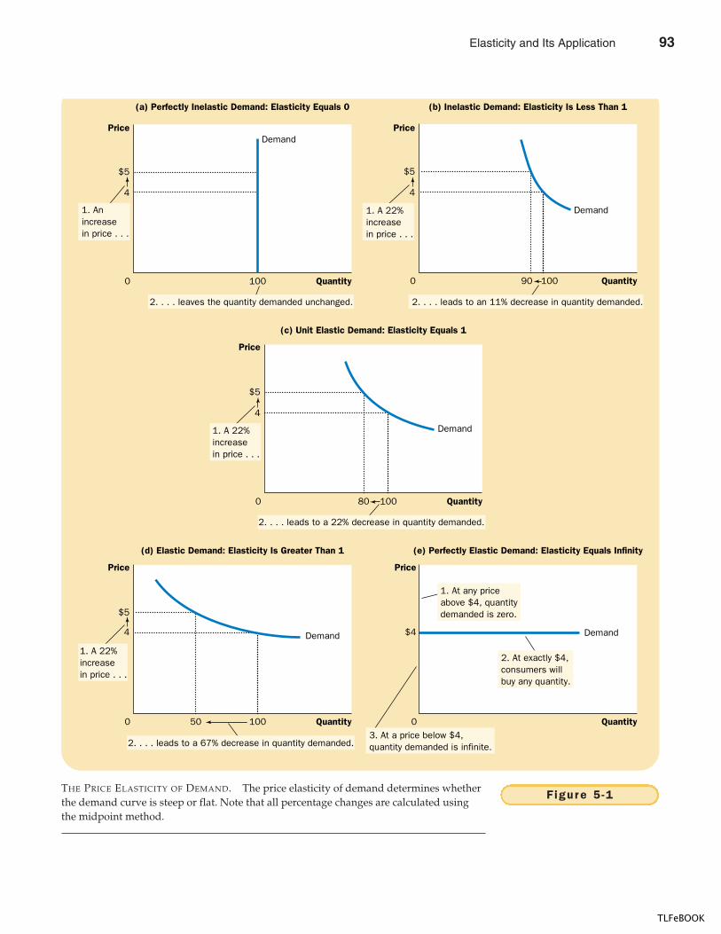
(a) Perfectly Inelastic Demand: Elasticity Equals 0
$5
4
Demand
Quantity1000
(b) Inelastic Demand: Elasticity Is Less Than 1
$5
4
Quantity1000 90
Demand
(c) Unit Elastic Demand: Elasticity Equals 1
$5
4
Demand
Quantity1000
Price
80
1. Anincreasein price . . .
2. . . . leaves the quantity demanded unchanged.
2. . . . leads to a 22% decrease in quantity demanded.
1. A 22%increasein price . . .
Price Price
2. . . . leads to an 11% decrease in quantity demanded.
1. A 22%increasein price . . .
(d) Elastic Demand: Elasticity Is Greater Than 1
$5
4 Demand
Quantity1000
Price
50
(e) Perfectly Elastic Demand: Elasticity Equals Infinity
$4
Quantity0
Price
Demand
1. A 22%increasein price . . .
2. At exactly $4,consumers willbuy any quantity.
1. At any priceabove $4, quantitydemanded is zero.
2. . . . leads to a 67% decrease in quantity demanded.3. At a price below $4,quantity demanded is infinite.
Figure 5 -1THE PRICE ELASTICITY OF DEMAND. The price elasticity of demand determines whetherthe demand curve is steep or flat. Note that all percentage changes are calculated usingthe midpoint method.
Elasticity and Its Application 93
TLFeBOOK
98 PART TWO SUPPLY AND DEMAND I : HOW MARKETS WORK
The numerator is the percentage change in quantity computed using the midpointmethod, and the denominator is the percentage change in price computed usingthe midpoint method. If you ever need to calculate elasticities, you should use thisformula.
Throughout this book, however, we only rarely need to perform such calcula-tions. For our purposes, what elasticity represents—the responsiveness of quantitydemanded to price—is more important than how it is calculated.
THE VARIETY OF DEMAND CURVES
Economists classify demand curves according to their elasticity. Demand is elasticwhen the elasticity is greater than 1, so that quantity moves proportionately morethan the price. Demand is inelastic when the elasticity is less than 1, so that quan-tity moves proportionately less than the price. If the elasticity is exactly 1, so thatquantity moves the same amount proportionately as price, demand is said to haveunit elasticity.
Because the price elasticity of demand measures how much quantity de-manded responds to changes in the price, it is closely related to the slope of the de-mand curve. The following rule of thumb is a useful guide: The flatter is thedemand curve that passes through a given point, the greater is the price elasticityof demand. The steeper is the demand curve that passes through a given point, thesmaller is the price elasticity of demand.
Figure 5-1 shows five cases. In the extreme case of a zero elasticity, demand isperfectly inelastic, and the demand curve is vertical. In this case, regardless of theprice, the quantity demanded stays the same. As the elasticity rises, the demandcurve gets flatter and flatter. At the opposite extreme, demand is perfectly elastic.This occurs as the price elasticity of demand approaches infinity and the demandcurve becomes horizontal, reflecting the fact that very small changes in the pricelead to huge changes in the quantity demanded.
Finally, if you have trouble keeping straight the terms elastic and inelastic,here’s a memory trick for you: Inelastic curves, such as in panel (a) of Figure 5-1,look like the letter I. Elastic curves, as in panel (e), look like the letter E. This is nota deep insight, but it might help on your next exam.
TOTAL REVENUE AND THE PRICE ELASTICITY OF DEMAND
When studying changes in supply or demand in a market, one variable we oftenwant to study is total revenue, the amount paid by buyers and received by sellersof the good. In any market, total revenue is P � Q, the price of the good times thequantity of the good sold. We can show total revenue graphically, as in Figure 5-2.The height of the box under the demand curve is P, and the width is Q. The areaof this box, P � Q, equals the total revenue in this market. In Figure 5-2, whereP � $4 and Q � 100, total revenue is $4 � 100, or $400.
How does total revenue change as one moves along the demand curve? Theanswer depends on the price elasticity of demand. If demand is inelastic, as in Fig-ure 5-3, then an increase in the price causes an increase in total revenue. Here anincrease in price from $1 to $3 causes the quantity demanded to fall only from 100
tota l r evenuethe amount paid by buyers andreceived by sellers of a good,computed as the price of the goodtimes the quantity sold
94 Elasticity and Its Application
TLFeBOOK
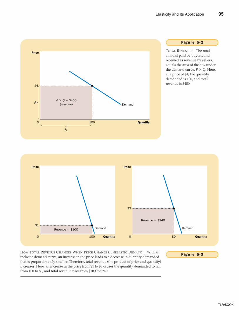
CHAPTER 5 ELASTICITY AND ITS APPLICATION 99
$4
Demand
Quantity
Q
P
0
Price
P � Q � $400(revenue)
100
Figure 5 -2
TOTAL REVENUE. The totalamount paid by buyers, andreceived as revenue by sellers,equals the area of the box underthe demand curve, P � Q. Here,at a price of $4, the quantitydemanded is 100, and totalrevenue is $400.
$1Demand
Quantity0
Price
Revenue � $100
100
$3
Quantity0
Price
80
Revenue � $240
Demand
Figure 5 -3HOW TOTAL REVENUE CHANGES WHEN PRICE CHANGES: INELASTIC DEMAND. With aninelastic demand curve, an increase in the price leads to a decrease in quantity demandedthat is proportionately smaller. Therefore, total revenue (the product of price and quantity)increases. Here, an increase in the price from $1 to $3 causes the quantity demanded to fallfrom 100 to 80, and total revenue rises from $100 to $240.
Elasticity and Its Application 95
TLFeBOOK
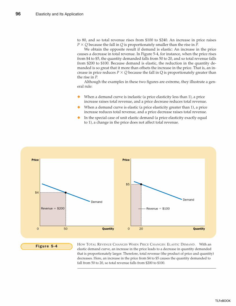
100 PART TWO SUPPLY AND DEMAND I : HOW MARKETS WORK
to 80, and so total revenue rises from $100 to $240. An increase in price raisesP � Q because the fall in Q is proportionately smaller than the rise in P.
We obtain the opposite result if demand is elastic: An increase in the pricecauses a decrease in total revenue. In Figure 5-4, for instance, when the price risesfrom $4 to $5, the quantity demanded falls from 50 to 20, and so total revenue fallsfrom $200 to $100. Because demand is elastic, the reduction in the quantity de-manded is so great that it more than offsets the increase in the price. That is, an in-crease in price reduces P � Q because the fall in Q is proportionately greater thanthe rise in P.
Although the examples in these two figures are extreme, they illustrate a gen-eral rule:
� When a demand curve is inelastic (a price elasticity less than 1), a priceincrease raises total revenue, and a price decrease reduces total revenue.
� When a demand curve is elastic (a price elasticity greater than 1), a priceincrease reduces total revenue, and a price decrease raises total revenue.
� In the special case of unit elastic demand (a price elasticity exactly equalto 1), a change in the price does not affect total revenue.
Demand
Quantity0
Price
Revenue � $200
$4
50
Demand
Quantity0
Price
Revenue � $100
$5
20
Figure 5 -4 HOW TOTAL REVENUE CHANGES WHEN PRICE CHANGES: ELASTIC DEMAND. With anelastic demand curve, an increase in the price leads to a decrease in quantity demandedthat is proportionately larger. Therefore, total revenue (the product of price and quantity)decreases. Here, an increase in the price from $4 to $5 causes the quantity demanded tofall from 50 to 20, so total revenue falls from $200 to $100.
96 Elasticity and Its Application
TLFeBOOK
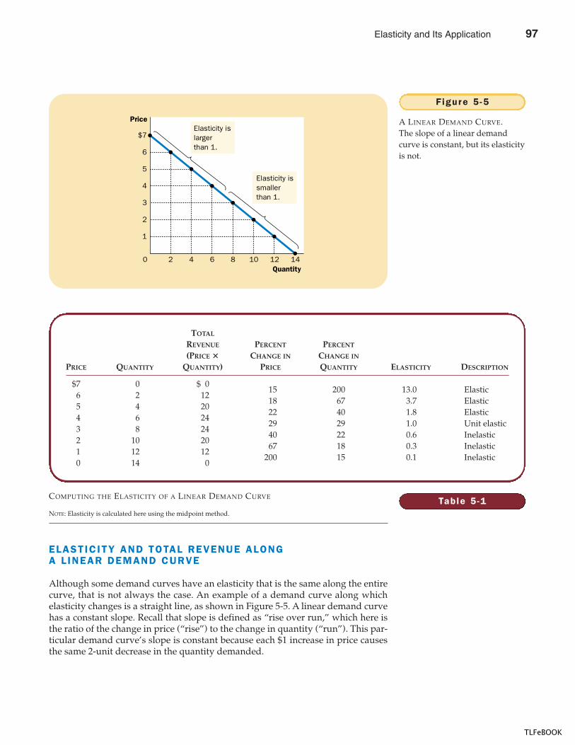
CHAPTER 5 ELASTICITY AND ITS APPLICATION 101
ELASTICITY AND TOTAL REVENUE ALONGA LINEAR DEMAND CURVE
Although some demand curves have an elasticity that is the same along the entirecurve, that is not always the case. An example of a demand curve along whichelasticity changes is a straight line, as shown in Figure 5-5. A linear demand curvehas a constant slope. Recall that slope is defined as “rise over run,” which here isthe ratio of the change in price (“rise”) to the change in quantity (“run”). This par-ticular demand curve’s slope is constant because each $1 increase in price causesthe same 2-unit decrease in the quantity demanded.
5
6
$7
4
1
2
3
Quantity122 4 6 8 10 140
PriceElasticity islargerthan 1.
Elasticity issmallerthan 1.
Figure 5 -5
A LINEAR DEMAND CURVE.The slope of a linear demandcurve is constant, but its elasticityis not.
Table 5 -1
TOTAL
REVENUE PERCENT PERCENT
(PRICE � CHANGE IN CHANGE IN
PRICE QUANTITY QUANTITY) PRICE QUANTITY ELASTICITY DESCRIPTION
$7 0 $ 015 200 13.0 Elastic
6 2 1218 67 3.7 Elastic
5 4 2022 40 1.8 Elastic
4 6 2429 29 1.0 Unit elastic
3 8 2440 22 0.6 Inelastic
2 10 2067 18 0.3 Inelastic
1 12 12200 15 0.1 Inelastic
0 14 0
COMPUTING THE ELASTICITY OF A LINEAR DEMAND CURVE
NOTE: Elasticity is calculated here using the midpoint method.
Elasticity and Its Application 97
TLFeBOOK
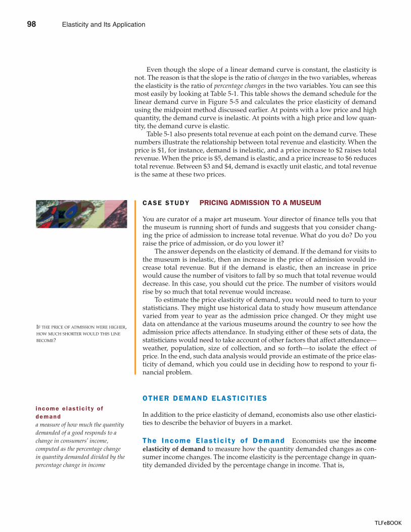
102 PART TWO SUPPLY AND DEMAND I : HOW MARKETS WORK
CASE STUDY PRICING ADMISSION TO A MUSEUM
You are curator of a major art museum. Your director of finance tells you thatthe museum is running short of funds and suggests that you consider chang-ing the price of admission to increase total revenue. What do you do? Do youraise the price of admission, or do you lower it?
The answer depends on the elasticity of demand. If the demand for visits tothe museum is inelastic, then an increase in the price of admission would in-crease total revenue. But if the demand is elastic, then an increase in pricewould cause the number of visitors to fall by so much that total revenue woulddecrease. In this case, you should cut the price. The number of visitors wouldrise by so much that total revenue would increase.
To estimate the price elasticity of demand, you would need to turn to yourstatisticians. They might use historical data to study how museum attendancevaried from year to year as the admission price changed. Or they might usedata on attendance at the various museums around the country to see how theadmission price affects attendance. In studying either of these sets of data, thestatisticians would need to take account of other factors that affect attendance—weather, population, size of collection, and so forth—to isolate the effect ofprice. In the end, such data analysis would provide an estimate of the price elas-ticity of demand, which you could use in deciding how to respond to your fi-nancial problem.
OTHER DEMAND ELASTICIT IES
In addition to the price elasticity of demand, economists also use other elastici-ties to describe the behavior of buyers in a market.
The Income E last ic i ty o f Demand Economists use the incomeelasticity of demand to measure how the quantity demanded changes as con-sumer income changes. The income elasticity is the percentage change in quan-tity demanded divided by the percentage change in income. That is,
Even though the slope of a linear demand curve is constant, the elasticity isnot. The reason is that the slope is the ratio of changes in the two variables, whereasthe elasticity is the ratio of percentage changes in the two variables. You can see thismost easily by looking at Table 5-1. This table shows the demand schedule for thelinear demand curve in Figure 5-5 and calculates the price elasticity of demandusing the midpoint method discussed earlier. At points with a low price and highquantity, the demand curve is inelastic. At points with a high price and low quan-tity, the demand curve is elastic.
Table 5-1 also presents total revenue at each point on the demand curve. Thesenumbers illustrate the relationship between total revenue and elasticity. When theprice is $1, for instance, demand is inelastic, and a price increase to $2 raises totalrevenue. When the price is $5, demand is elastic, and a price increase to $6 reducestotal revenue. Between $3 and $4, demand is exactly unit elastic, and total revenueis the same at these two prices.
IF THE PRICE OF ADMISSION WERE HIGHER,HOW MUCH SHORTER WOULD THIS LINE
BECOME?
income e last ic i ty o fdemanda measure of how much the quantitydemanded of a good responds to achange in consumers’ income,computed as the percentage changein quantity demanded divided by thepercentage change in income
98 Elasticity and Its Application
TLFeBOOK
CHAPTER 5 ELASTICITY AND ITS APPLICATION 103
Income elasticity of demand � .
As we discussed in Chapter 4, most goods are normal goods: Higher income raisesquantity demanded. Because quantity demanded and income move in the samedirection, normal goods have positive income elasticities. A few goods, such as bus
Percentage change in quantity demandedPercentage change in income
HOW SHOULD A FIRM THAT OPERATES A
private toll road set a price for its ser-vice? As the following article makesclear, answering this question requiresan understanding of the demand curveand its elasticity.
F o r W h o m t h e B o o t h To l l s ,P r i c e R e a l l y D o e s M a t t e r
BY STEVEN PEARLSTEIN
All businesses face a similar question:What price for their product will generatethe maximum profit?
The answer is not always obvious:Raising the price of something often hasthe effect of reducing sales as price-sensitive consumers seek alternatives orsimply do without. For every product, theextent of that sensitivity is different. Thetrick is to find the point for each wherethe ideal tradeoff between profit marginand sales volume is achieved.
Right now, the developers of a newprivate toll road between Leesburg and
Washington-Dulles International Airportare trying to discern the magic point. Thegroup originally projected that it couldcharge nearly $2 for the 14-mile one-waytrip, while attracting 34,000 trips on anaverage day from overcrowded publicroads such as nearby Route 7. But afterspending $350 million to build their muchheralded “Greenway,” they discoveredto their dismay that only about a thirdthat number of commuters were willingto pay that much to shave 20 minutes offtheir daily commute. . . .
It was only when the company, indesperation, lowered the toll to $1 that itcame even close to attracting the ex-pected traffic flows.
Although the Greenway still is los-ing money, it is clearly better off at thisnew point on the demand curve than itwas when it first opened. Average dailyrevenue today is $22,000, comparedwith $14,875 when the “special intro-ductory” price was $1.75. And with traf-fic still light even at rush hour, it ispossible that the owners may lower tollseven further in search of higher revenue.
After all, when the price was low-ered by 45 percent last spring, it gener-ated a 200 percent increase in volumethree months later. If the same ratio ap-plies again, lowering the toll another25 percent would drive the daily volumeup to 38,000 trips, and daily revenue upto nearly $29,000.
The problem, of course, is that thesame ratio usually does not apply at
every price point, which is why this pric-ing business is so tricky. . . .
Clifford Winston of the BrookingsInstitution and John Calfee of the Ameri-can Enterprise Institute have consideredthe toll road’s dilemma. . . .
Last year, the economists con-ducted an elaborate market test with1,170 people across the country whowere each presented with a series of op-tions in which they were, in effect, askedto make a personal tradeoff betweenless commuting time and higher tolls.
In the end, they concluded that thepeople who placed the highest value onreducing their commuting time alreadyhad done so by finding public transporta-tion, living closer to their work, or select-ing jobs that allowed them to commuteat off-peak hours.
Conversely, those who commutedsignificant distances had a higher toler-ance for traffic congestion and were will-ing to pay only 20 percent of their hourlypay to save an hour of their time.
Overall, the Winston/Calfee find-ings help explain why the Greenway’soriginal toll and volume projections weretoo high: By their reckoning, only com-muters who earned at least $30 an hour(about $60,000 a year) would be willingto pay $2 to save 20 minutes.
SOURCE: The Washington Post, October 24, 1996,p. E1.
IN THE NEWS
On the Roadwith Elasticity
Elasticity and Its Application 99
TLFeBOOK
104 PART TWO SUPPLY AND DEMAND I : HOW MARKETS WORK
rides, are inferior goods: Higher income lowers the quantity demanded. Becausequantity demanded and income move in opposite directions, inferior goods havenegative income elasticities.
Even among normal goods, income elasticities vary substantially in size. Ne-cessities, such as food and clothing, tend to have small income elasticities becauseconsumers, regardless of how low their incomes, choose to buy some of thesegoods. Luxuries, such as caviar and furs, tend to have large income elasticities be-cause consumers feel that they can do without these goods altogether if their in-come is too low.
The Cross -P r ice E last ic i ty o f Demand Economists use the cross-price elasticity of demand to measure how the quantity demanded of one goodchanges as the price of another good changes. It is calculated as the percentagechange in quantity demanded of good 1 divided by the percentage change in theprice of good 2. That is,
Cross-price elasticity of demand � .
Whether the cross-price elasticity is a positive or negative number depends onwhether the two goods are substitutes or complements. As we discussed in Chap-ter 4, substitutes are goods that are typically used in place of one another, such ashamburgers and hot dogs. An increase in hot dog prices induces people to grillhamburgers instead. Because the price of hot dogs and the quantity of hamburgersdemanded move in the same direction, the cross-price elasticity is positive. Con-versely, complements are goods that are typically used together, such as comput-ers and software. In this case, the cross-price elasticity is negative, indicating thatan increase in the price of computers reduces the quantity of software demanded.
QUICK QUIZ: Define the price elasticity of demand. � Explain the relationship between total revenue and the price elasticity of demand.
THE ELASTICITY OF SUPPLY
When we discussed the determinants of supply in Chapter 4, we noted that sellersof a good increase the quantity supplied when the price of the good rises, whentheir input prices fall, or when their technology improves. To turn from qualita-tive to quantitative statements about supply, we once again use the concept ofelasticity.
THE PRICE ELASTICITY OF SUPPLYAND ITS DETERMINANTS
The law of supply states that higher prices raise the quantity supplied. The priceelasticity of supply measures how much the quantity supplied responds tochanges in the price. Supply of a good is said to be elastic if the quantity supplied
Percentage change in quantitydemanded of good 1Percentage change in
the price of good 2
cross -p r ice e last ic i ty o fdemanda measure of how much the quantitydemanded of one good responds to achange in the price of another good,computed as the percentage changein quantity demanded of the firstgood divided by the percentagechange in the price of the secondgood
pr ice e last ic i ty o f supp lya measure of how much the quantitysupplied of a good responds to achange in the price of that good,computed as the percentage changein quantity supplied divided by thepercentage change in price
100 Elasticity and Its Application
TLFeBOOK
CHAPTER 5 ELASTICITY AND ITS APPLICATION 105
responds substantially to changes in the price. Supply is said to be inelastic if thequantity supplied responds only slightly to changes in the price.
The price elasticity of supply depends on the flexibility of sellers to change theamount of the good they produce. For example, beachfront land has an inelasticsupply because it is almost impossible to produce more of it. By contrast, manu-factured goods, such as books, cars, and televisions, have elastic supplies becausethe firms that produce them can run their factories longer in response to a higherprice.
In most markets, a key determinant of the price elasticity of supply is the timeperiod being considered. Supply is usually more elastic in the long run than in theshort run. Over short periods of time, firms cannot easily change the size of theirfactories to make more or less of a good. Thus, in the short run, the quantity sup-plied is not very responsive to the price. By contrast, over longer periods, firms canbuild new factories or close old ones. In addition, new firms can enter a market,and old firms can shut down. Thus, in the long run, the quantity supplied can re-spond substantially to the price.
COMPUTING THE PRICE ELASTICITY OF SUPPLY
Now that we have some idea about what the price elasticity of supply is, let’s bemore precise. Economists compute the price elasticity of supply as the percentagechange in the quantity supplied divided by the percentage change in the price.That is,
Price elasticity of supply � .
For example, suppose that an increase in the price of milk from $2.85 to $3.15 a gal-lon raises the amount that dairy farmers produce from 9,000 to 11,000 gallons permonth. Using the midpoint method, we calculate the percentage change in price as
Percentage change in price � (3.15 � 2.85)/3.00 � 100 � 10 percent.
Similarly, we calculate the percentage change in quantity supplied as
Percentage change in quantity supplied � (11,000 � 9,000)/10,000 � 100� 20 percent.
In this case, the price elasticity of supply is
Price elasticity of supply � � 2.0.
In this example, the elasticity of 2 reflects the fact that the quantity supplied movesproportionately twice as much as the price.
THE VARIETY OF SUPPLY CURVES
Because the price elasticity of supply measures the responsiveness of quantity sup-plied to the price, it is reflected in the appearance of the supply curve. Figure 5-6shows five cases. In the extreme case of a zero elasticity, supply is perfectly inelastic,
20 percent10 percent
Percentage change in quantity suppliedPercentage change in price
Elasticity and Its Application 101
TLFeBOOK
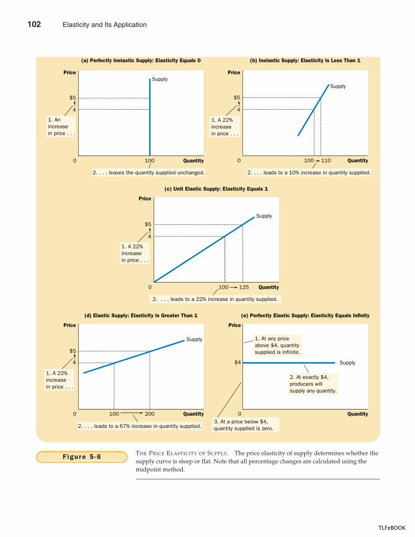
100 110
100 125
(a) Perfectly Inelastic Supply: Elasticity Equals 0
$5
4
Supply
Quantity1000
(b) Inelastic Supply: Elasticity Is Less Than 1
$5
4
Quantity0
(c) Unit Elastic Supply: Elasticity Equals 1
$5
4
Quantity0
Price
1. Anincreasein price . . .
2. . . . leaves the quantity supplied unchanged.
2. . . . leads to a 22% increase in quantity supplied.
1. A 22%increasein price . . .
Price Price
2. . . . leads to a 10% increase in quantity supplied.
1. A 22%increasein price . . .
(d) Elastic Supply: Elasticity Is Greater Than 1
$5
4
Quantity0
Price
(e) Perfectly Elastic Supply: Elasticity Equals Infinity
$4
Quantity0
Price
Supply
1. A 22%increasein price . . .
2. At exactly $4,producers willsupply any quantity.
1. At any priceabove $4, quantitysupplied is infinite.
2. . . . leads to a 67% increase in quantity supplied.3. At a price below $4,quantity supplied is zero.
Supply
Supply
100 200
Supply
Figure 5 -6 THE PRICE ELASTICITY OF SUPPLY. The price elasticity of supply determines whether thesupply curve is steep or flat. Note that all percentage changes are calculated using themidpoint method.
102 Elasticity and Its Application
TLFeBOOK
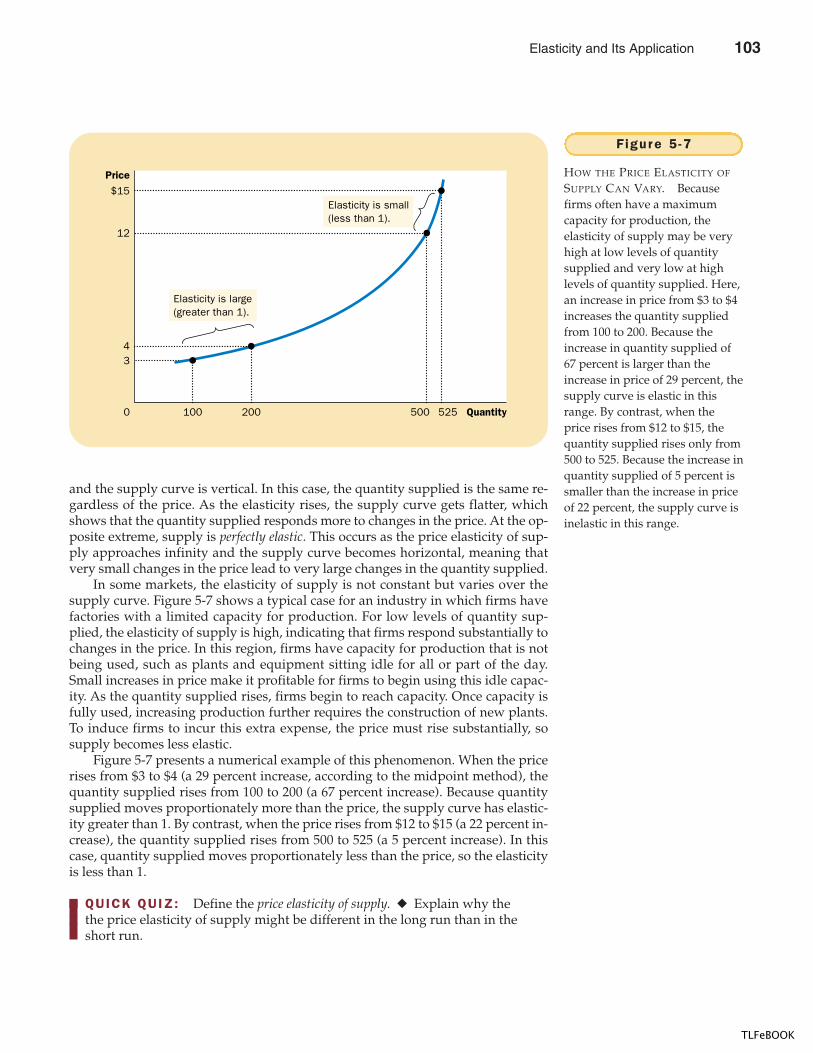
CHAPTER 5 ELASTICITY AND ITS APPLICATION 107
and the supply curve is vertical. In this case, the quantity supplied is the same re-gardless of the price. As the elasticity rises, the supply curve gets flatter, whichshows that the quantity supplied responds more to changes in the price. At the op-posite extreme, supply is perfectly elastic. This occurs as the price elasticity of sup-ply approaches infinity and the supply curve becomes horizontal, meaning thatvery small changes in the price lead to very large changes in the quantity supplied.
In some markets, the elasticity of supply is not constant but varies over thesupply curve. Figure 5-7 shows a typical case for an industry in which firms havefactories with a limited capacity for production. For low levels of quantity sup-plied, the elasticity of supply is high, indicating that firms respond substantially tochanges in the price. In this region, firms have capacity for production that is notbeing used, such as plants and equipment sitting idle for all or part of the day.Small increases in price make it profitable for firms to begin using this idle capac-ity. As the quantity supplied rises, firms begin to reach capacity. Once capacity isfully used, increasing production further requires the construction of new plants.To induce firms to incur this extra expense, the price must rise substantially, sosupply becomes less elastic.
Figure 5-7 presents a numerical example of this phenomenon. When the pricerises from $3 to $4 (a 29 percent increase, according to the midpoint method), thequantity supplied rises from 100 to 200 (a 67 percent increase). Because quantitysupplied moves proportionately more than the price, the supply curve has elastic-ity greater than 1. By contrast, when the price rises from $12 to $15 (a 22 percent in-crease), the quantity supplied rises from 500 to 525 (a 5 percent increase). In thiscase, quantity supplied moves proportionately less than the price, so the elasticityis less than 1.
QUICK QUIZ: Define the price elasticity of supply. � Explain why the the price elasticity of supply might be different in the long run than in the short run.
$15
12
3
Quantity100 200 5000
Price
525
Elasticity is small(less than 1).
Elasticity is large(greater than 1).
4
Figure 5 -7
HOW THE PRICE ELASTICITY OF
SUPPLY CAN VARY. Becausefirms often have a maximumcapacity for production, theelasticity of supply may be veryhigh at low levels of quantitysupplied and very low at highlevels of quantity supplied. Here,an increase in price from $3 to $4increases the quantity suppliedfrom 100 to 200. Because theincrease in quantity supplied of67 percent is larger than theincrease in price of 29 percent, thesupply curve is elastic in thisrange. By contrast, when theprice rises from $12 to $15, thequantity supplied rises only from500 to 525. Because the increase inquantity supplied of 5 percent issmaller than the increase in priceof 22 percent, the supply curve isinelastic in this range.
Elasticity and Its Application 103
TLFeBOOK
108 PART TWO SUPPLY AND DEMAND I : HOW MARKETS WORK
THREE APPLICATIONS OF SUPPLY,DEMAND, AND ELASTICITY
Can good news for farming be bad news for farmers? Why did the Organization ofPetroleum Exporting Countries (OPEC) fail to keep the price of oil high? Doesdrug interdiction increase or decrease drug-related crime? At first, these questionsmight seem to have little in common. Yet all three questions are about markets,and all markets are subject to the forces of supply and demand. Here we apply theversatile tools of supply, demand, and elasticity to answer these seemingly com-plex questions.
CAN GOOD NEWS FOR FARMING BEBAD NEWS FOR FARMERS?
Let’s now return to the question posed at the beginning of this chapter: What hap-pens to wheat farmers and the market for wheat when university agronomists dis-cover a new wheat hybrid that is more productive than existing varieties? Recallfrom Chapter 4 that we answer such questions in three steps. First, we examinewhether the supply curve or demand curve shifts. Second, we consider which di-rection the curve shifts. Third, we use the supply-and-demand diagram to see howthe market equilibrium changes.
In this case, the discovery of the new hybrid affects the supply curve. Becausethe hybrid increases the amount of wheat that can be produced on each acre ofland, farmers are now willing to supply more wheat at any given price. In otherwords, the supply curve shifts to the right. The demand curve remains the samebecause consumers’ desire to buy wheat products at any given price is not affectedby the introduction of a new hybrid. Figure 5-8 shows an example of such achange. When the supply curve shifts from S1 to S2, the quantity of wheat sold in-creases from 100 to 110, and the price of wheat falls from $3 to $2.
But does this discovery make farmers better off? As a first cut to answeringthis question, consider what happens to the total revenue received by farmers.Farmers’ total revenue is P � Q, the price of the wheat times the quantity sold. Thediscovery affects farmers in two conflicting ways. The hybrid allows farmers toproduce more wheat (Q rises), but now each bushel of wheat sells for less (P falls).
Whether total revenue rises or falls depends on the elasticity of demand. Inpractice, the demand for basic foodstuffs such as wheat is usually inelastic, forthese items are relatively inexpensive and have few good substitutes. When thedemand curve is inelastic, as it is in Figure 5-8, a decrease in price causes total rev-enue to fall. You can see this in the figure: The price of wheat falls substantially,whereas the quantity of wheat sold rises only slightly. Total revenue falls from$300 to $220. Thus, the discovery of the new hybrid lowers the total revenue thatfarmers receive for the sale of their crops.
If farmers are made worse off by the discovery of this new hybrid, why dothey adopt it? The answer to this question goes to the heart of how competitivemarkets work. Because each farmer is a small part of the market for wheat, he orshe takes the price of wheat as given. For any given price of wheat, it is better to
104 Elasticity and Its Application
TLFeBOOK
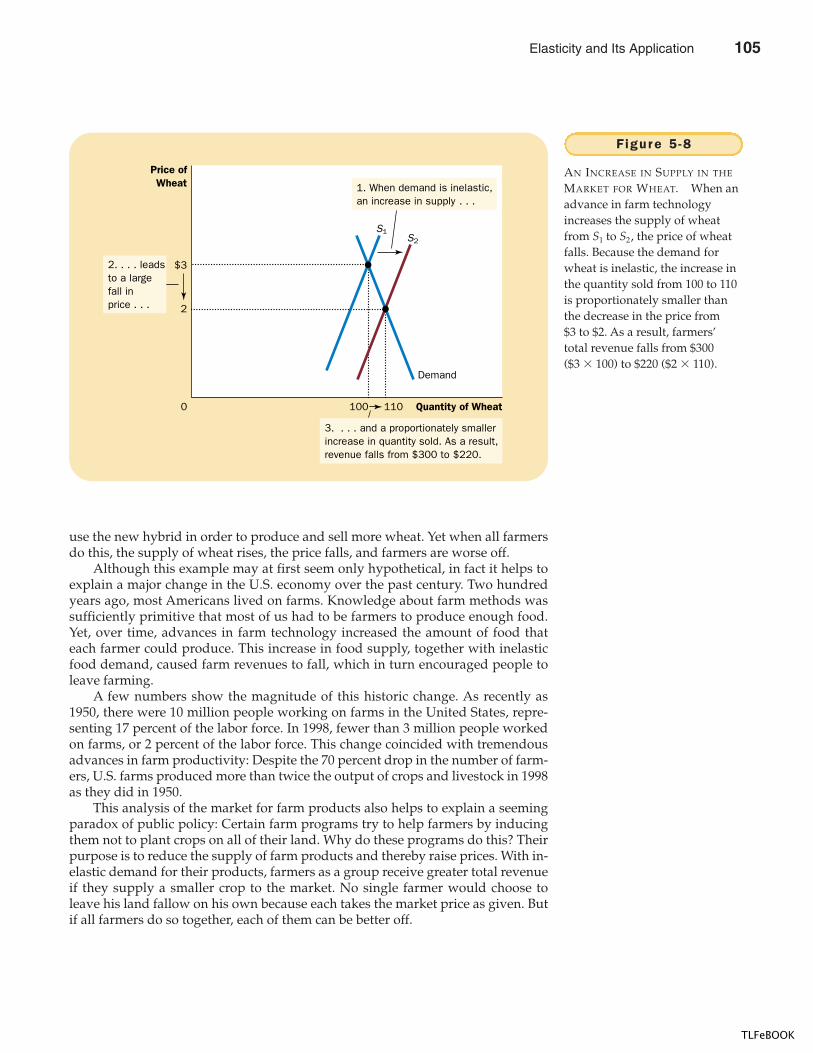
CHAPTER 5 ELASTICITY AND ITS APPLICATION 109
use the new hybrid in order to produce and sell more wheat. Yet when all farmersdo this, the supply of wheat rises, the price falls, and farmers are worse off.
Although this example may at first seem only hypothetical, in fact it helps toexplain a major change in the U.S. economy over the past century. Two hundredyears ago, most Americans lived on farms. Knowledge about farm methods wassufficiently primitive that most of us had to be farmers to produce enough food.Yet, over time, advances in farm technology increased the amount of food thateach farmer could produce. This increase in food supply, together with inelasticfood demand, caused farm revenues to fall, which in turn encouraged people toleave farming.
A few numbers show the magnitude of this historic change. As recently as1950, there were 10 million people working on farms in the United States, repre-senting 17 percent of the labor force. In 1998, fewer than 3 million people workedon farms, or 2 percent of the labor force. This change coincided with tremendousadvances in farm productivity: Despite the 70 percent drop in the number of farm-ers, U.S. farms produced more than twice the output of crops and livestock in 1998as they did in 1950.
This analysis of the market for farm products also helps to explain a seemingparadox of public policy: Certain farm programs try to help farmers by inducingthem not to plant crops on all of their land. Why do these programs do this? Theirpurpose is to reduce the supply of farm products and thereby raise prices. With in-elastic demand for their products, farmers as a group receive greater total revenueif they supply a smaller crop to the market. No single farmer would choose toleave his land fallow on his own because each takes the market price as given. Butif all farmers do so together, each of them can be better off.
$3
2
Quantity of Wheat1000
Price ofWheat 1. When demand is inelastic,
an increase in supply . . .
3. . . . and a proportionately smallerincrease in quantity sold. As a result,revenue falls from $300 to $220.
110
Demand
S1S2
2. . . . leadsto a largefall inprice . . .
Figure 5 -8
AN INCREASE IN SUPPLY IN THE
MARKET FOR WHEAT. When anadvance in farm technologyincreases the supply of wheatfrom S1 to S2, the price of wheatfalls. Because the demand forwheat is inelastic, the increase inthe quantity sold from 100 to 110is proportionately smaller thanthe decrease in the price from$3 to $2. As a result, farmers’total revenue falls from $300($3 � 100) to $220 ($2 � 110).
Elasticity and Its Application 105
TLFeBOOK
110 PART TWO SUPPLY AND DEMAND I : HOW MARKETS WORK
When analyzing the effects of farm technology or farm policy, it is importantto keep in mind that what is good for farmers is not necessarily good for society asa whole. Improvement in farm technology can be bad for farmers who become in-creasingly unnecessary, but it is surely good for consumers who pay less for food.Similarly, a policy aimed at reducing the supply of farm products may raise the in-comes of farmers, but it does so at the expense of consumers.
WHY DID OPEC FAIL TO KEEP THE PRICE OF OIL HIGH?
Many of the most disruptive events for the world’s economies over the past sev-eral decades have originated in the world market for oil. In the 1970s members ofthe Organization of Petroleum Exporting Countries (OPEC) decided to raise theworld price of oil in order to increase their incomes. These countries accomplishedthis goal by jointly reducing the amount of oil they supplied. From 1973 to 1974,the price of oil (adjusted for overall inflation) rose more than 50 percent. Then, afew years later, OPEC did the same thing again. The price of oil rose 14 percent in1979, followed by 34 percent in 1980, and another 34 percent in 1981.
Yet OPEC found it difficult to maintain a high price. From 1982 to 1985, theprice of oil steadily declined at about 10 percent per year. Dissatisfaction and dis-array soon prevailed among the OPEC countries. In 1986 cooperation amongOPEC members completely broke down, and the price of oil plunged 45 percent.In 1990 the price of oil (adjusted for overall inflation) was back to where it beganin 1970, and it has stayed at that low level throughout most of the 1990s.
This episode shows how supply and demand can behave differently in theshort run and in the long run. In the short run, both the supply and demand for oilare relatively inelastic. Supply is inelastic because the quantity of known oil re-serves and the capacity for oil extraction cannot be changed quickly. Demand is in-elastic because buying habits do not respond immediately to changes in price.Many drivers with old gas-guzzling cars, for instance, will just pay the higher
106 Elasticity and Its Application
TLFeBOOK
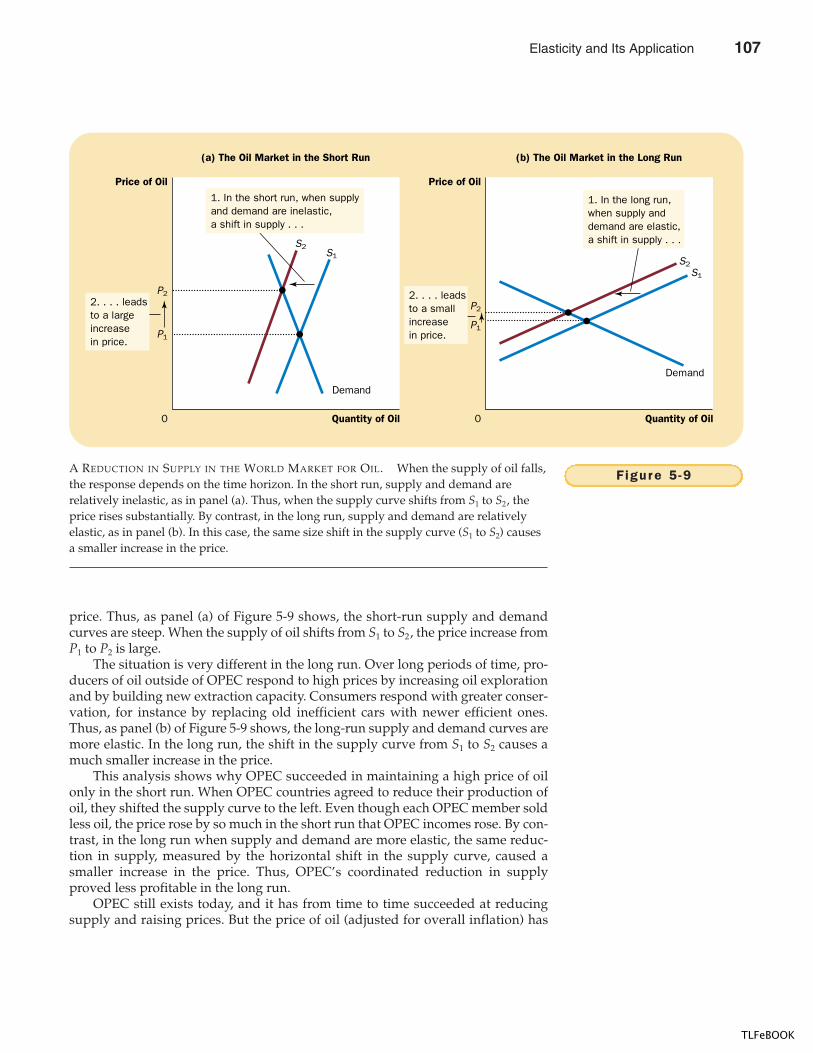
CHAPTER 5 ELASTICITY AND ITS APPLICATION 111
price. Thus, as panel (a) of Figure 5-9 shows, the short-run supply and demandcurves are steep. When the supply of oil shifts from S1 to S2, the price increase fromP1 to P2 is large.
The situation is very different in the long run. Over long periods of time, pro-ducers of oil outside of OPEC respond to high prices by increasing oil explorationand by building new extraction capacity. Consumers respond with greater conser-vation, for instance by replacing old inefficient cars with newer efficient ones.Thus, as panel (b) of Figure 5-9 shows, the long-run supply and demand curves aremore elastic. In the long run, the shift in the supply curve from S1 to S2 causes amuch smaller increase in the price.
This analysis shows why OPEC succeeded in maintaining a high price of oilonly in the short run. When OPEC countries agreed to reduce their production ofoil, they shifted the supply curve to the left. Even though each OPEC member soldless oil, the price rose by so much in the short run that OPEC incomes rose. By con-trast, in the long run when supply and demand are more elastic, the same reduc-tion in supply, measured by the horizontal shift in the supply curve, caused asmaller increase in the price. Thus, OPEC’s coordinated reduction in supplyproved less profitable in the long run.
OPEC still exists today, and it has from time to time succeeded at reducingsupply and raising prices. But the price of oil (adjusted for overall inflation) has
P2
P1
Quantity of Oil0
Price of Oil
Demand
S2S1
(a) The Oil Market in the Short Run
P2
P1
Quantity of Oil0
Price of Oil
Demand
S2S1
(b) The Oil Market in the Long Run
2. . . . leadsto a largeincreasein price.
1. In the long run,when supply anddemand are elastic,a shift in supply . . .
2. . . . leadsto a smallincreasein price.
1. In the short run, when supplyand demand are inelastic,a shift in supply . . .
Figure 5 -9A REDUCTION IN SUPPLY IN THE WORLD MARKET FOR OIL. When the supply of oil falls,the response depends on the time horizon. In the short run, supply and demand arerelatively inelastic, as in panel (a). Thus, when the supply curve shifts from S1 to S2, theprice rises substantially. By contrast, in the long run, supply and demand are relativelyelastic, as in panel (b). In this case, the same size shift in the supply curve (S1 to S2) causesa smaller increase in the price.
Elasticity and Its Application 107
TLFeBOOK
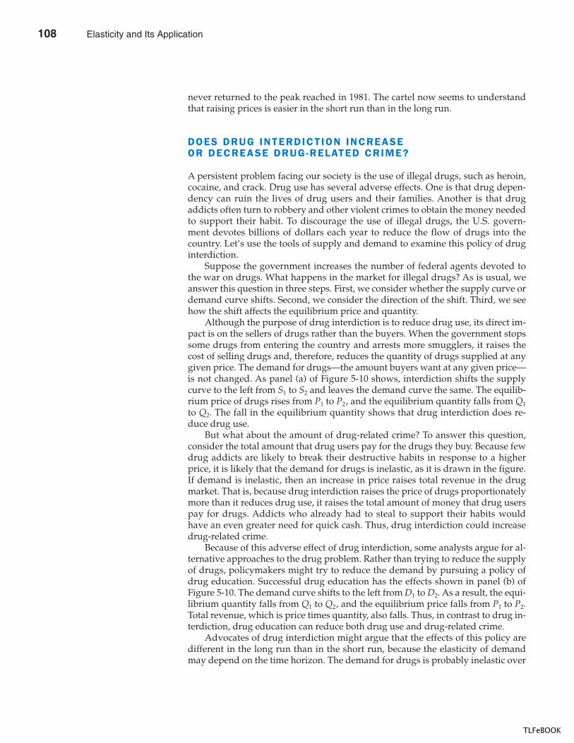
112 PART TWO SUPPLY AND DEMAND I : HOW MARKETS WORK
never returned to the peak reached in 1981. The cartel now seems to understandthat raising prices is easier in the short run than in the long run.
DOES DRUG INTERDICTION INCREASEOR DECREASE DRUG-RELATED CRIME?
A persistent problem facing our society is the use of illegal drugs, such as heroin,cocaine, and crack. Drug use has several adverse effects. One is that drug depen-dency can ruin the lives of drug users and their families. Another is that drugaddicts often turn to robbery and other violent crimes to obtain the money neededto support their habit. To discourage the use of illegal drugs, the U.S. govern-ment devotes billions of dollars each year to reduce the flow of drugs into thecountry. Let’s use the tools of supply and demand to examine this policy of druginterdiction.
Suppose the government increases the number of federal agents devoted tothe war on drugs. What happens in the market for illegal drugs? As is usual, weanswer this question in three steps. First, we consider whether the supply curve ordemand curve shifts. Second, we consider the direction of the shift. Third, we seehow the shift affects the equilibrium price and quantity.
Although the purpose of drug interdiction is to reduce drug use, its direct im-pact is on the sellers of drugs rather than the buyers. When the government stopssome drugs from entering the country and arrests more smugglers, it raises thecost of selling drugs and, therefore, reduces the quantity of drugs supplied at anygiven price. The demand for drugs—the amount buyers want at any given price—is not changed. As panel (a) of Figure 5-10 shows, interdiction shifts the supplycurve to the left from S1 to S2 and leaves the demand curve the same. The equilib-rium price of drugs rises from P1 to P2, and the equilibrium quantity falls from Q1
to Q2. The fall in the equilibrium quantity shows that drug interdiction does re-duce drug use.
But what about the amount of drug-related crime? To answer this question,consider the total amount that drug users pay for the drugs they buy. Because fewdrug addicts are likely to break their destructive habits in response to a higherprice, it is likely that the demand for drugs is inelastic, as it is drawn in the figure.If demand is inelastic, then an increase in price raises total revenue in the drugmarket. That is, because drug interdiction raises the price of drugs proportionatelymore than it reduces drug use, it raises the total amount of money that drug userspay for drugs. Addicts who already had to steal to support their habits wouldhave an even greater need for quick cash. Thus, drug interdiction could increasedrug-related crime.
Because of this adverse effect of drug interdiction, some analysts argue for al-ternative approaches to the drug problem. Rather than trying to reduce the supplyof drugs, policymakers might try to reduce the demand by pursuing a policy ofdrug education. Successful drug education has the effects shown in panel (b) ofFigure 5-10. The demand curve shifts to the left from D1 to D2. As a result, the equi-librium quantity falls from Q1 to Q2, and the equilibrium price falls from P1 to P2.Total revenue, which is price times quantity, also falls. Thus, in contrast to drug in-terdiction, drug education can reduce both drug use and drug-related crime.
Advocates of drug interdiction might argue that the effects of this policy aredifferent in the long run than in the short run, because the elasticity of demandmay depend on the time horizon. The demand for drugs is probably inelastic over
108 Elasticity and Its Application
TLFeBOOK
CHAPTER 5 ELASTICITY AND ITS APPLICATION 113
short periods of time because higher prices do not substantially affect drug use byestablished addicts. But demand may be more elastic over longer periods of timebecause higher prices would discourage experimentation with drugs among theyoung and, over time, lead to fewer drug addicts. In this case, drug interdic-tion would increase drug-related crime in the short run while decreasing it in thelong run.
QUICK QUIZ: How might a drought that destroys half of all farm crops be good for farmers? If such a drought is good for farmers, why don’t farmers destroy their own crops in the absence of a drought?
CONCLUSION
According to an old quip, even a parrot can become an economist simply by learn-ing to say “supply and demand.” These last two chapters should have convincedyou that there is much truth in this statement. The tools of supply and demandallow you to analyze many of the most important events and policies that shape
P2
P1
Quantity of Drugs0 Q2 Q1
Price ofDrugs
Demand
S2
S1
Q2 Q1
(a) Drug Interdiction
Quantity of Drugs0
Price ofDrugs
Supply
D2
D1
(b) Drug Education
3. . . . and reduces the quantity sold.
2. . . . whichraises theprice . . .
2. . . . whichreduces the price . . .
P1
P2
1. Drug interdiction reducesthe supply of drugs . . .
1. Drug education reducesthe demand for drugs . . .
3. . . . and reduces the quantity sold.
Figure 5 -10POLICIES TO REDUCE THE USE OF ILLEGAL DRUGS. Drug interdiction reduces the supplyof drugs from S1 to S2, as in panel (a). If the demand for drugs is inelastic, then the totalamount paid by drug users rises, even as the amount of drug use falls. By contrast, drugeducation reduces the demand for drugs from D1 to D2, as in panel (b). Because both priceand quantity fall, the amount paid by drug users falls.
Elasticity and Its Application 109
TLFeBOOK
114 PART TWO SUPPLY AND DEMAND I : HOW MARKETS WORK
the economy. You are now well on your way to becoming an economist (or, at least,a well-educated parrot).
� The price elasticity of demand measures how much thequantity demanded responds to changes in the price.Demand tends to be more elastic if the good is a luxuryrather than a necessity, if close substitutes are available,if the market is narrowly defined, or if buyers havesubstantial time to react to a price change.
� The price elasticity of demand is calculated as thepercentage change in quantity demanded divided bythe percentage change in price. If the elasticity is lessthan 1, so that quantity demanded movesproportionately less than the price, demand is said to beinelastic. If the elasticity is greater than 1, so thatquantity demanded moves proportionately more thanthe price, demand is said to be elastic.
� Total revenue, the total amount paid for a good, equalsthe price of the good times the quantity sold. Forinelastic demand curves, total revenue rises as pricerises. For elastic demand curves, total revenue falls asprice rises.
� The income elasticity of demand measures how muchthe quantity demanded responds to changes in
consumers’ income. The cross-price elasticity of demandmeasures how much the quantity demanded of onegood responds to the price of another good.
� The price elasticity of supply measures how much thequantity supplied responds to changes in the price. Thiselasticity often depends on the time horizon underconsideration. In most markets, supply is more elastic inthe long run than in the short run.
� The price elasticity of supply is calculated as thepercentage change in quantity supplied divided by thepercentage change in price. If the elasticity is less than 1,so that quantity supplied moves proportionately lessthan the price, supply is said to be inelastic. If theelasticity is greater than 1, so that quantity suppliedmoves proportionately more than the price, supply issaid to be elastic.
� The tools of supply and demand can be applied in manydifferent kinds of markets. This chapter uses them toanalyze the market for wheat, the market for oil, and themarket for illegal drugs.
Summar y
elasticity, p. 94price elasticity of demand, p. 94
total revenue, p. 98income elasticity of demand, p. 102
cross-price elasticity of demand, p. 104price elasticity of supply, p. 104
Key Concepts
1. Define the price elasticity of demand and the incomeelasticity of demand.
2. List and explain some of the determinants of the priceelasticity of demand.
3. If the elasticity is greater than 1, is demand elastic orinelastic? If the elasticity equals 0, is demand perfectlyelastic or perfectly inelastic?
4. On a supply-and-demand diagram, show equilibriumprice, equilibrium quantity, and the total revenuereceived by producers.
5. If demand is elastic, how will an increase in pricechange total revenue? Explain.
6. What do we call a good whose income elasticity is lessthan 0?
7. How is the price elasticity of supply calculated? Explainwhat this measures.
8. What is the price elasticity of supply of Picassopaintings?
9. Is the price elasticity of supply usually larger in theshort run or in the long run? Why?
10. In the 1970s, OPEC caused a dramatic increase in theprice of oil. What prevented it from maintaining thishigh price through the 1980s?
Quest ions fo r Rev iew
110 Elasticity and Its Application
TLFeBOOK
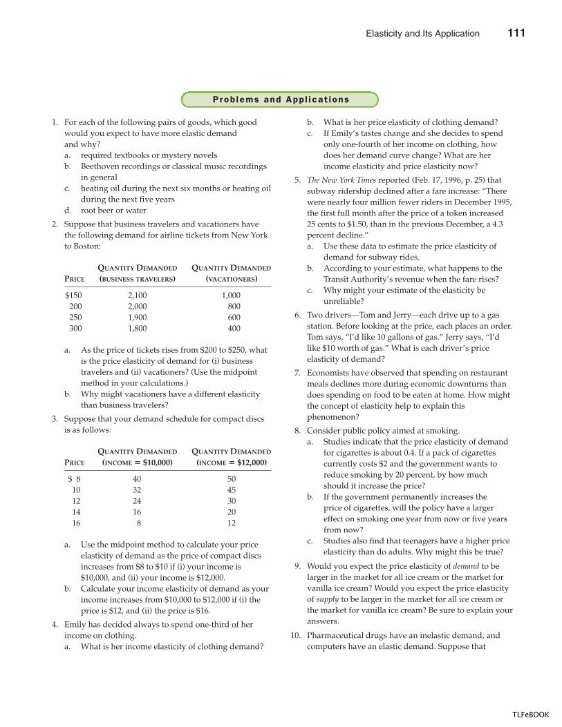
CHAPTER 5 ELASTICITY AND ITS APPLICATION 115
1. For each of the following pairs of goods, which goodwould you expect to have more elastic demandand why?a. required textbooks or mystery novelsb. Beethoven recordings or classical music recordings
in generalc. heating oil during the next six months or heating oil
during the next five yearsd. root beer or water
2. Suppose that business travelers and vacationers havethe following demand for airline tickets from New Yorkto Boston:
QUANTITY DEMANDED QUANTITY DEMANDED
PRICE (BUSINESS TRAVELERS) (VACATIONERS)
$150 2,100 1,000200 2,000 800250 1,900 600300 1,800 400
a. As the price of tickets rises from $200 to $250, whatis the price elasticity of demand for (i) businesstravelers and (ii) vacationers? (Use the midpointmethod in your calculations.)
b. Why might vacationers have a different elasticitythan business travelers?
3. Suppose that your demand schedule for compact discsis as follows:
QUANTITY DEMANDED QUANTITY DEMANDED
PRICE (INCOME � $10,000) (INCOME � $12,000)
$ 8 40 5010 32 4512 24 3014 16 2016 8 12
a. Use the midpoint method to calculate your priceelasticity of demand as the price of compact discsincreases from $8 to $10 if (i) your income is$10,000, and (ii) your income is $12,000.
b. Calculate your income elasticity of demand as yourincome increases from $10,000 to $12,000 if (i) theprice is $12, and (ii) the price is $16.
4. Emily has decided always to spend one-third of herincome on clothing.a. What is her income elasticity of clothing demand?
b. What is her price elasticity of clothing demand?c. If Emily’s tastes change and she decides to spend
only one-fourth of her income on clothing, howdoes her demand curve change? What are herincome elasticity and price elasticity now?
5. The New York Times reported (Feb. 17, 1996, p. 25) thatsubway ridership declined after a fare increase: “Therewere nearly four million fewer riders in December 1995,the first full month after the price of a token increased25 cents to $1.50, than in the previous December, a 4.3percent decline.”a. Use these data to estimate the price elasticity of
demand for subway rides.b. According to your estimate, what happens to the
Transit Authority’s revenue when the fare rises?c. Why might your estimate of the elasticity be
unreliable?
6. Two drivers—Tom and Jerry—each drive up to a gasstation. Before looking at the price, each places an order.Tom says, “I’d like 10 gallons of gas.” Jerry says, “I’dlike $10 worth of gas.” What is each driver’s priceelasticity of demand?
7. Economists have observed that spending on restaurantmeals declines more during economic downturns thandoes spending on food to be eaten at home. How mightthe concept of elasticity help to explain thisphenomenon?
8. Consider public policy aimed at smoking.a. Studies indicate that the price elasticity of demand
for cigarettes is about 0.4. If a pack of cigarettescurrently costs $2 and the government wants toreduce smoking by 20 percent, by how muchshould it increase the price?
b. If the government permanently increases theprice of cigarettes, will the policy have a largereffect on smoking one year from now or five yearsfrom now?
c. Studies also find that teenagers have a higher priceelasticity than do adults. Why might this be true?
9. Would you expect the price elasticity of demand to belarger in the market for all ice cream or the market forvanilla ice cream? Would you expect the price elasticityof supply to be larger in the market for all ice cream orthe market for vanilla ice cream? Be sure to explain youranswers.
10. Pharmaceutical drugs have an inelastic demand, andcomputers have an elastic demand. Suppose that
Prob lems and App l icat ions
Elasticity and Its Application 111
TLFeBOOK
116 PART TWO SUPPLY AND DEMAND I : HOW MARKETS WORK
technological advance doubles the supply of bothproducts (that is, the quantity supplied at each price istwice what it was).a. What happens to the equilibrium price and
quantity in each market?b. Which product experiences a larger change in
price?c. Which product experiences a larger change in
quantity?d. What happens to total consumer spending on each
product?
11. Beachfront resorts have an inelastic supply, andautomobiles have an elastic supply. Suppose that a risein population doubles the demand for both products(that is, the quantity demanded at each price is twicewhat it was).a. What happens to the equilibrium price and
quantity in each market?b. Which product experiences a larger change in
price?c. Which product experiences a larger change in
quantity?d. What happens to total consumer spending on each
product?
12. Several years ago, flooding along the Missouri andMississippi rivers destroyed thousands of acres ofwheat.
a. Farmers whose crops were destroyed by the floodswere much worse off, but farmers whose cropswere not destroyed benefited from the floods.Why?
b. What information would you need about themarket for wheat in order to assess whetherfarmers as a group were hurt or helped by thefloods?
13. Explain why the following might be true: A droughtaround the world raises the total revenue that farmersreceive from the sale of grain, but a drought only inKansas reduces the total revenue that Kansas farmersreceive.
14. Because better weather makes farmland moreproductive, farmland in regions with good weatherconditions is more expensive than farmland in regionswith bad weather conditions. Over time, however, asadvances in technology have made all farmland moreproductive, the price of farmland (adjusted for overallinflation) has fallen. Use the concept of elasticity toexplain why productivity and farmland prices arepositively related across space but negatively relatedover time.
112 Elasticity and Its Application
TLFeBOOK
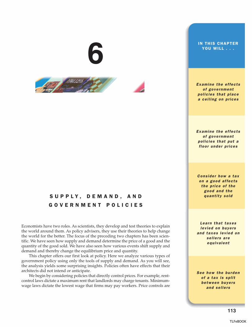
IN THIS CHAPTERYOU WILL . . .
See how the burdenof a tax is sp l i tbetween buyers
and se l le rs
Cons ider how a taxon a good a f fectsthe pr ice o f the
good and thequant i ty so ld
Examine the e f fectsof government
po l ic ies that p lacea ce i l ing on pr ices
Examine the e f fectsof government
po l ic ies that put af loor under p r ices
Learn that taxeslev ied on buyers
and taxes lev ied onse l le rs a reequ iva lent
Economists have two roles. As scientists, they develop and test theories to explainthe world around them. As policy advisers, they use their theories to help changethe world for the better. The focus of the preceding two chapters has been scien-tific. We have seen how supply and demand determine the price of a good and thequantity of the good sold. We have also seen how various events shift supply anddemand and thereby change the equilibrium price and quantity.
This chapter offers our first look at policy. Here we analyze various types ofgovernment policy using only the tools of supply and demand. As you will see,the analysis yields some surprising insights. Policies often have effects that theirarchitects did not intend or anticipate.
We begin by considering policies that directly control prices. For example, rent-control laws dictate a maximum rent that landlords may charge tenants. Minimum-wage laws dictate the lowest wage that firms may pay workers. Price controls are
S U P P L Y , D E M A N D , A N D
G O V E R N M E N T P O L I C I E S
117
113
6
TLFeBOOK
118 PART TWO SUPPLY AND DEMAND I : HOW MARKETS WORK
usually enacted when policymakers believe that the market price of a good or ser-vice is unfair to buyers or sellers. Yet, as we will see, these policies can generate in-equities of their own.
After our discussion of price controls, we next consider the impact of taxes.Policymakers use taxes both to influence market outcomes and to raise revenue forpublic purposes. Although the prevalence of taxes in our economy is obvious,their effects are not. For example, when the government levies a tax on the amountthat firms pay their workers, do the firms or the workers bear the burden of thetax? The answer is not at all clear—until we apply the powerful tools of supplyand demand.
CONTROLS ON PRICES
To see how price controls affect market outcomes, let’s look once again at the mar-ket for ice cream. As we saw in Chapter 4, if ice cream is sold in a competitive mar-ket free of government regulation, the price of ice cream adjusts to balance supplyand demand: At the equilibrium price, the quantity of ice cream that buyers wantto buy exactly equals the quantity that sellers want to sell. To be concrete, supposethe equilibrium price is $3 per cone.
Not everyone may be happy with the outcome of this free-market process.Let’s say the American Association of Ice Cream Eaters complains that the $3 priceis too high for everyone to enjoy a cone a day (their recommended diet). Mean-while, the National Organization of Ice Cream Makers complains that the $3price—the result of “cutthroat competition”—is depressing the incomes of itsmembers. Each of these groups lobbies the government to pass laws that alter themarket outcome by directly controlling prices.
Of course, because buyers of any good always want a lower price while sellerswant a higher price, the interests of the two groups conflict. If the Ice Cream Eatersare successful in their lobbying, the government imposes a legal maximum on theprice at which ice cream can be sold. Because the price is not allowed to rise abovethis level, the legislated maximum is called a price ceiling. By contrast, if the IceCream Makers are successful, the government imposes a legal minimum on theprice. Because the price cannot fall below this level, the legislated minimum iscalled a price floor. Let us consider the effects of these policies in turn.
HOW PRICE CEIL INGS AFFECT MARKET OUTCOMES
When the government, moved by the complaints of the Ice Cream Eaters, imposesa price ceiling on the market for ice cream, two outcomes are possible. In panel (a)of Figure 6-1, the government imposes a price ceiling of $4 per cone. In this case,because the price that balances supply and demand ($3) is below the ceiling, theprice ceiling is not binding. Market forces naturally move the economy to the equi-librium, and the price ceiling has no effect.
Panel (b) of Figure 6-1 shows the other, more interesting, possibility. In this case,the government imposes a price ceiling of $2 per cone. Because the equilibriumprice of $3 is above the price ceiling, the ceiling is a binding constraint on the market.
pr ice ce i l inga legal maximum on the price atwhich a good can be sold
pr ice f loora legal minimum on the price atwhich a good can be sold
114 Supply, Demand, and Government Policies
TLFeBOOK
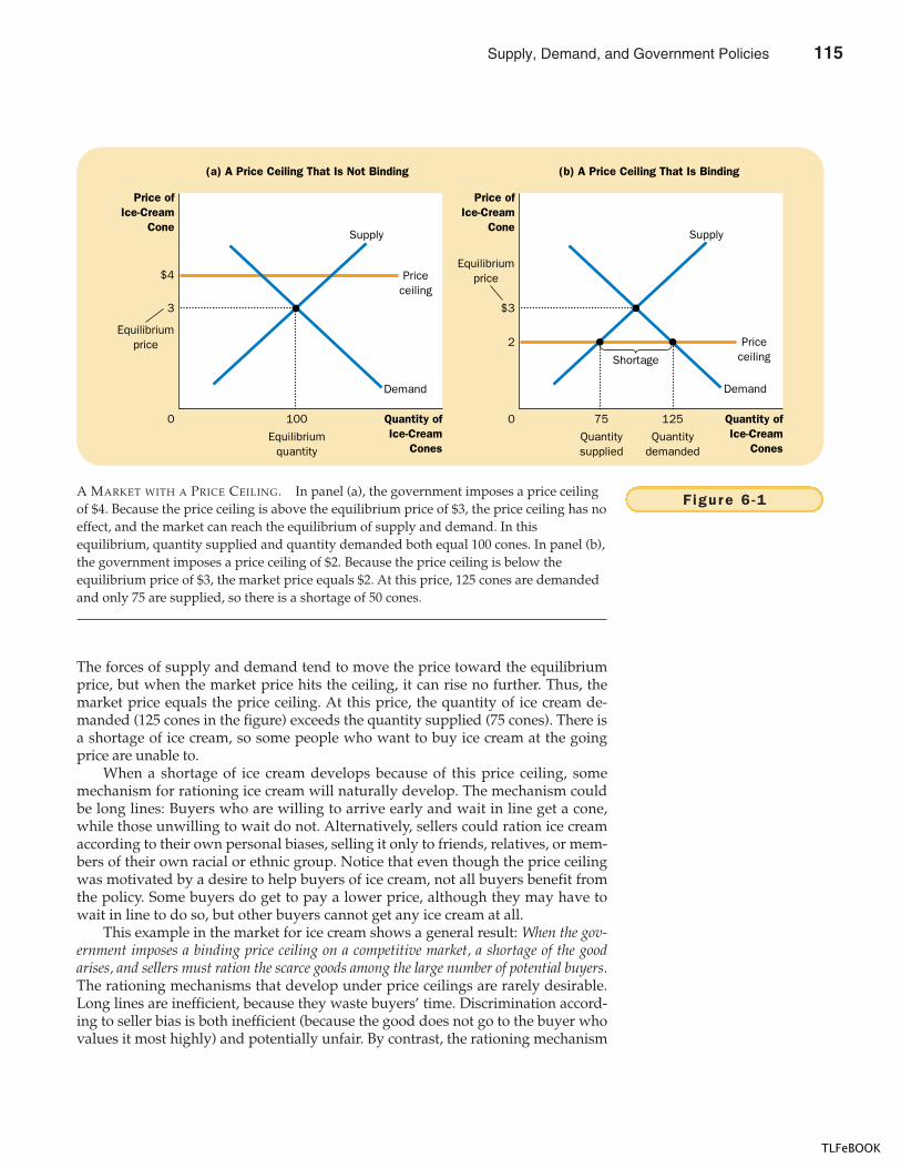
CHAPTER 6 SUPPLY, DEMAND, AND GOVERNMENT POLICIES 119
The forces of supply and demand tend to move the price toward the equilibriumprice, but when the market price hits the ceiling, it can rise no further. Thus, themarket price equals the price ceiling. At this price, the quantity of ice cream de-manded (125 cones in the figure) exceeds the quantity supplied (75 cones). There isa shortage of ice cream, so some people who want to buy ice cream at the goingprice are unable to.
When a shortage of ice cream develops because of this price ceiling, somemechanism for rationing ice cream will naturally develop. The mechanism couldbe long lines: Buyers who are willing to arrive early and wait in line get a cone,while those unwilling to wait do not. Alternatively, sellers could ration ice creamaccording to their own personal biases, selling it only to friends, relatives, or mem-bers of their own racial or ethnic group. Notice that even though the price ceilingwas motivated by a desire to help buyers of ice cream, not all buyers benefit fromthe policy. Some buyers do get to pay a lower price, although they may have towait in line to do so, but other buyers cannot get any ice cream at all.
This example in the market for ice cream shows a general result: When the gov-ernment imposes a binding price ceiling on a competitive market, a shortage of the goodarises, and sellers must ration the scarce goods among the large number of potential buyers.The rationing mechanisms that develop under price ceilings are rarely desirable.Long lines are inefficient, because they waste buyers’ time. Discrimination accord-ing to seller bias is both inefficient (because the good does not go to the buyer whovalues it most highly) and potentially unfair. By contrast, the rationing mechanism
(a) A Price Ceiling That Is Not Binding
$4
3
Quantity ofIce-Cream
Cones
0
Price ofIce-Cream
Cone
100
Equilibriumquantity
(b) A Price Ceiling That Is Binding
$3
Quantity ofIce-Cream
Cones
0
Price ofIce-Cream
Cone
2
Priceceiling
Demand
Supply
PriceceilingShortage
75
Quantitysupplied
125
Quantitydemanded
Equilibriumprice
Equilibriumprice
Demand
Supply
Figure 6 -1A MARKET WITH A PRICE CEILING. In panel (a), the government imposes a price ceilingof $4. Because the price ceiling is above the equilibrium price of $3, the price ceiling has noeffect, and the market can reach the equilibrium of supply and demand. In thisequilibrium, quantity supplied and quantity demanded both equal 100 cones. In panel (b),the government imposes a price ceiling of $2. Because the price ceiling is below theequilibrium price of $3, the market price equals $2. At this price, 125 cones are demandedand only 75 are supplied, so there is a shortage of 50 cones.
Supply, Demand, and Government Policies 115
TLFeBOOK
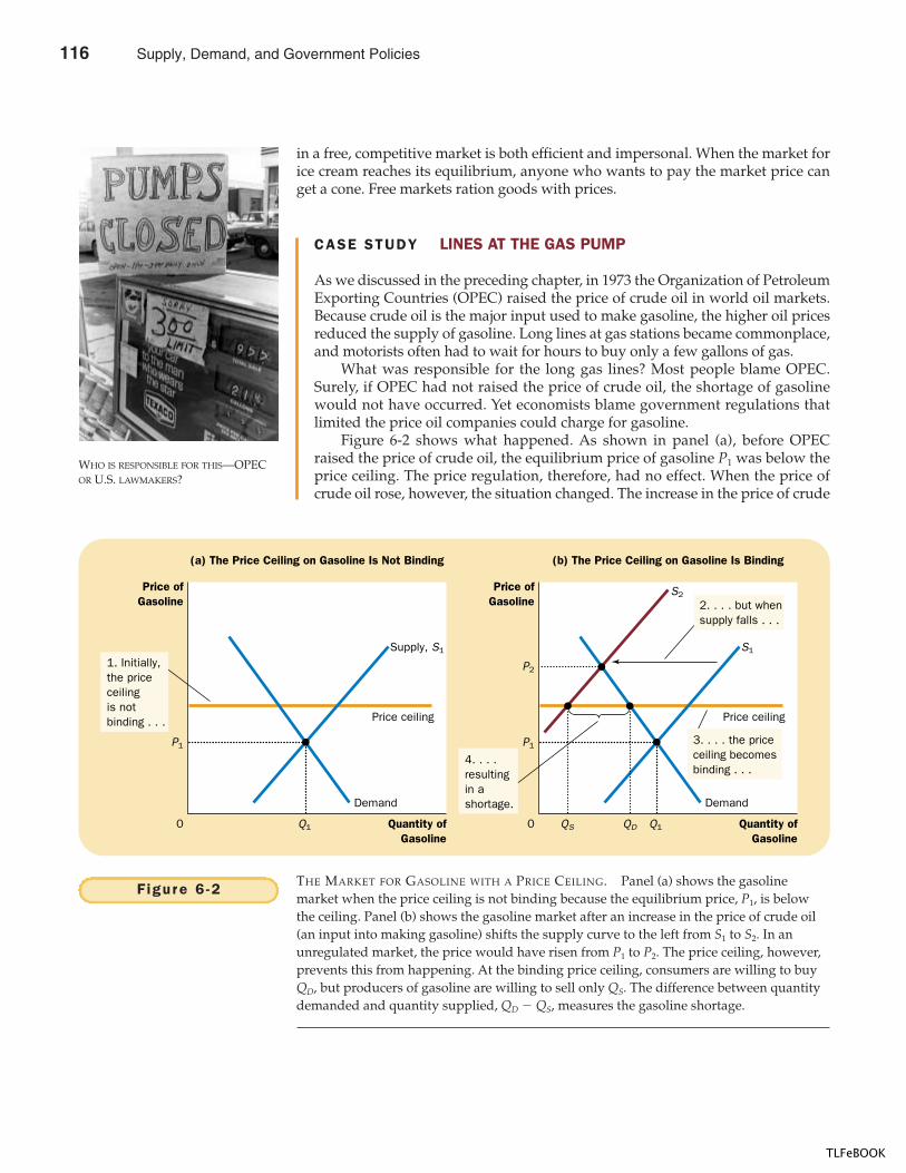
120 PART TWO SUPPLY AND DEMAND I : HOW MARKETS WORK
CASE STUDY LINES AT THE GAS PUMP
As we discussed in the preceding chapter, in 1973 the Organization of PetroleumExporting Countries (OPEC) raised the price of crude oil in world oil markets.Because crude oil is the major input used to make gasoline, the higher oil pricesreduced the supply of gasoline. Long lines at gas stations became commonplace,and motorists often had to wait for hours to buy only a few gallons of gas.
What was responsible for the long gas lines? Most people blame OPEC.Surely, if OPEC had not raised the price of crude oil, the shortage of gasolinewould not have occurred. Yet economists blame government regulations thatlimited the price oil companies could charge for gasoline.
Figure 6-2 shows what happened. As shown in panel (a), before OPECraised the price of crude oil, the equilibrium price of gasoline P1 was below theprice ceiling. The price regulation, therefore, had no effect. When the price ofcrude oil rose, however, the situation changed. The increase in the price of crude
in a free, competitive market is both efficient and impersonal. When the market forice cream reaches its equilibrium, anyone who wants to pay the market price canget a cone. Free markets ration goods with prices.
WHO IS RESPONSIBLE FOR THIS—OPECOR U.S. LAWMAKERS?
(a) The Price Ceiling on Gasoline Is Not Binding
Quantity ofGasoline
0
Price ofGasoline
(b) The Price Ceiling on Gasoline Is Binding
P2
P1
Quantity ofGasoline
0
Price ofGasoline
Q1QD
Demand
S1
S2
Price ceiling
QS
4. . . . resultingin ashortage.
3. . . . the priceceiling becomesbinding . . .
2. . . . but whensupply falls . . .
1. Initially,the priceceilingis notbinding . . . Price ceiling
P1
Q1
Demand
Supply, S1
Figure 6 -2THE MARKET FOR GASOLINE WITH A PRICE CEILING. Panel (a) shows the gasolinemarket when the price ceiling is not binding because the equilibrium price, P1, is belowthe ceiling. Panel (b) shows the gasoline market after an increase in the price of crude oil(an input into making gasoline) shifts the supply curve to the left from S1 to S2. In anunregulated market, the price would have risen from P1 to P2. The price ceiling, however,prevents this from happening. At the binding price ceiling, consumers are willing to buyQD, but producers of gasoline are willing to sell only QS. The difference between quantitydemanded and quantity supplied, QD � QS, measures the gasoline shortage.
116 Supply, Demand, and Government Policies
TLFeBOOK
CHAPTER 6 SUPPLY, DEMAND, AND GOVERNMENT POLICIES 121
oil raised the cost of producing gasoline, and this reduced the supply of gaso-line. As panel (b) shows, the supply curve shifted to the left from S1 to S2. In anunregulated market, this shift in supply would have raised the equilibriumprice of gasoline from P1 to P2, and no shortage would have resulted. Instead,the price ceiling prevented the price from rising to the equilibrium level. At the
DURING THE SUMMER OF 1999, THE EAST
coast of the United States experiencedunusually little rain and a shortage ofwater. The following article suggests away that the shortage could have beenaverted.
Tr i c k l e - D o w n E c o n o m i c s
BY TERRY L. ANDERSON AND
CLAY J. LANDRY
Water shortages are being blamed onthe drought in the East, but that’s givingMother Nature a bum rap. Certainly thedrought is the immediate cause, but thereal culprit is regulations that don’t allowmarkets and prices to equalize demandand supply.
The similarity between water andgasoline is instructive. The energy crisisof the 1970s, too, was blamed on na-ture’s niggardly supply of oil, but in factit was the actions of the Organizationof Petroleum Exporting Countries, com-bined with price controls, that was themain cause of the shortages. . . .
Once again, regulators are respond-ing to shortages—in this case of water—with controls and regulations rather thanallowing the market to work. Cities arerestricting water usage; some have evengone so far as to prohibit restaurantsfrom serving water except if the cus-tomer asks for a glass. But althoughcities initially saw declines in water use,some are starting to report increases inconsumption. This has prompted somepolice departments to collect lists of res-idents suspected of wasting water.
There’s a better answer than send-ing out the cops. Market forces couldensure plentiful water availability even indrought years. Contrary to popular be-lief, the supply of water is no more fixedthan the supply of oil. Like all resources,water supplies change in response toeconomic growth and to the price. In de-veloping countries, despite populationgrowth, the percentage of people withaccess to safe drinking water has in-creased to 74 percent in 1994 from 44percent in 1980. Rising incomes havegiven those countries the wherewithal tosupply potable water.
Supplies also increase when currentusers have an incentive to conserve theirsurplus in the marketplace. California’sdrought-emergency water bank illus-trates this. The bank allows farmers tolease water from other users during dryspells. In 1991, the first year the bankwas tried, when the price was $125 peracre-foot (326,000 gallons), supply ex-ceeded demand by two to one. That is,
many more people wanted to sell theirwater than wanted to buy.
Data from every corner of the worldshow that when cities raise the price ofwater by 10 percent, water use goesdown by as much as 12 percent. Whenthe price of agricultural water goes up10 percent, usage goes down by 20percent. . . .
Unfortunately, Eastern water usersdo not pay realistic prices for water.According to the American WaterWorks Association, only 2 percent ofmunicipal water suppliers adjust pricesseasonally. . . .
Even more egregious, Eastern waterlaws bar people from buying and sellingwater. Just as tradable pollution permitsestablished under the Clean Air Act haveencouraged polluters to find efficientways to reduce emissions, tradable waterrights can encourage conservation and in-crease supplies. It is mainly a matter offollowing the lead of Western watercourts that have quantified water rightsand Western legislatures that have al-lowed trades.
By making water a commodity andunleashing market forces, policymakerscan ensure plentiful water supplies forall. New policies won’t make droughtsdisappear, but they will ease the painthey impose by priming the invisiblepump of water markets.
SOURCE: The Wall Street Journal, August 23, 1999,p. A14.
IN THE NEWS
Does a Drought Need toCause a Water Shortage?
Supply, Demand, and Government Policies 117
TLFeBOOK
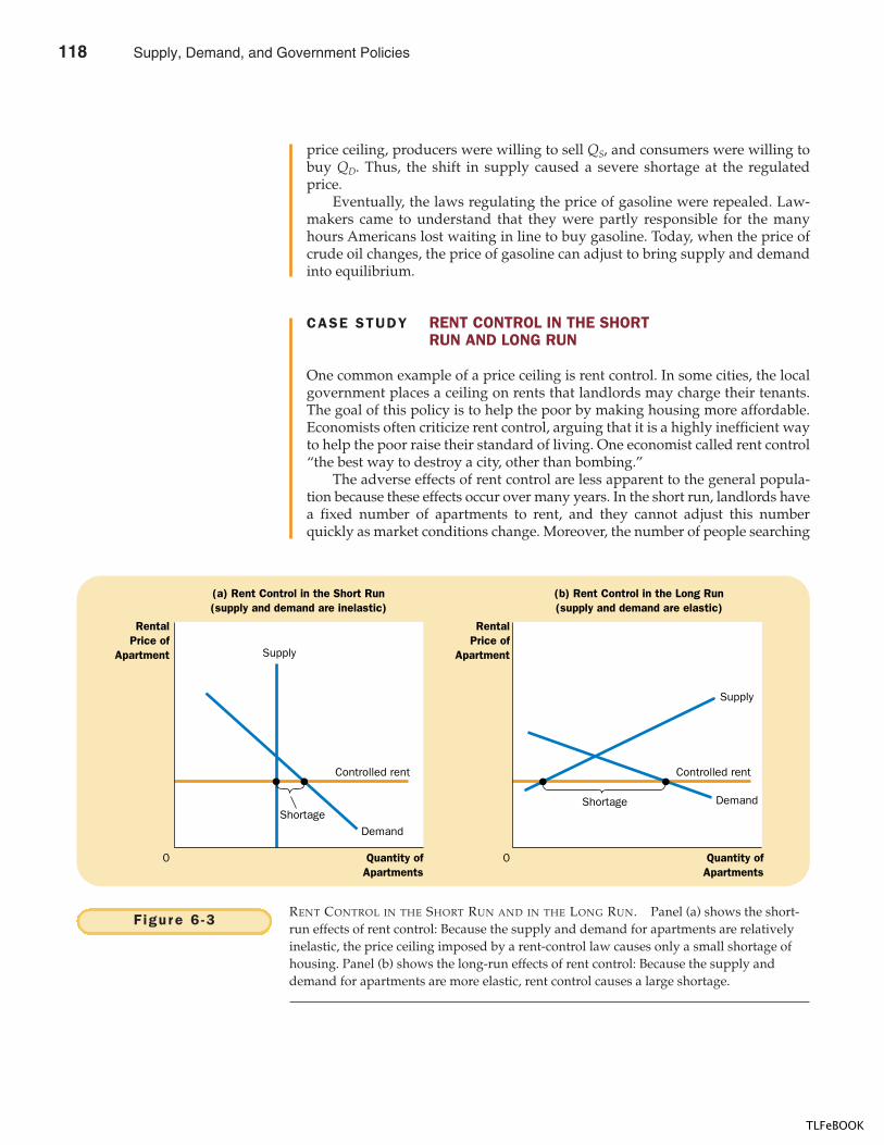
122 PART TWO SUPPLY AND DEMAND I : HOW MARKETS WORK
price ceiling, producers were willing to sell QS, and consumers were willing tobuy QD. Thus, the shift in supply caused a severe shortage at the regulatedprice.
Eventually, the laws regulating the price of gasoline were repealed. Law-makers came to understand that they were partly responsible for the manyhours Americans lost waiting in line to buy gasoline. Today, when the price ofcrude oil changes, the price of gasoline can adjust to bring supply and demandinto equilibrium.
CASE STUDY RENT CONTROL IN THE SHORTRUN AND LONG RUN
One common example of a price ceiling is rent control. In some cities, the localgovernment places a ceiling on rents that landlords may charge their tenants.The goal of this policy is to help the poor by making housing more affordable.Economists often criticize rent control, arguing that it is a highly inefficient wayto help the poor raise their standard of living. One economist called rent control“the best way to destroy a city, other than bombing.”
The adverse effects of rent control are less apparent to the general popula-tion because these effects occur over many years. In the short run, landlords havea fixed number of apartments to rent, and they cannot adjust this numberquickly as market conditions change. Moreover, the number of people searching
(a) Rent Control in the Short Run(supply and demand are inelastic)
(b) Rent Control in the Long Run(supply and demand are elastic)
Quantity ofApartments
0
Supply
Controlled rent
Shortage
RentalPrice of
Apartment
0
RentalPrice of
Apartment
Quantity ofApartments
Demand
Supply
Controlled rent
Shortage
Demand
Figure 6 -3RENT CONTROL IN THE SHORT RUN AND IN THE LONG RUN. Panel (a) shows the short-run effects of rent control: Because the supply and demand for apartments are relativelyinelastic, the price ceiling imposed by a rent-control law causes only a small shortage ofhousing. Panel (b) shows the long-run effects of rent control: Because the supply anddemand for apartments are more elastic, rent control causes a large shortage.
118 Supply, Demand, and Government Policies
TLFeBOOK
CHAPTER 6 SUPPLY, DEMAND, AND GOVERNMENT POLICIES 123
for housing in a city may not be highly responsive to rents in the short run be-cause people take time to adjust their housing arrangements. Therefore, theshort-run supply and demand for housing are relatively inelastic.
Panel (a) of Figure 6-3 shows the short-run effects of rent control on thehousing market. As with any price ceiling, rent control causes a shortage. Yetbecause supply and demand are inelastic in the short run, the initial shortagecaused by rent control is small. The primary effect in the short run is to reducerents.
The long-run story is very different because the buyers and sellers of rentalhousing respond more to market conditions as time passes. On the supply side,landlords respond to low rents by not building new apartments and by failingto maintain existing ones. On the demand side, low rents encourage people tofind their own apartments (rather than living with their parents or sharingapartments with roommates) and induce more people to move into a city.Therefore, both supply and demand are more elastic in the long run.
Panel (b) of Figure 6-3 illustrates the housing market in the long run. Whenrent control depresses rents below the equilibrium level, the quantity of apart-ments supplied falls substantially, and the quantity of apartments demandedrises substantially. The result is a large shortage of housing.
In cities with rent control, landlords use various mechanisms to ration hous-ing. Some landlords keep long waiting lists. Others give a preference to tenantswithout children. Still others discriminate on the basis of race. Sometimes, apart-ments are allocated to those willing to offer under-the-table payments to buildingsuperintendents. In essence, these bribes bring the total price of an apartment (in-cluding the bribe) closer to the equilibrium price.
To understand fully the effects of rent control, we have to remember one ofthe Ten Principles of Economics from Chapter 1: People respond to incentives. Infree markets, landlords try to keep their buildings clean and safe because desir-able apartments command higher prices. By contrast, when rent control createsshortages and waiting lists, landlords lose their incentive to be responsive totenants’ concerns. Why should a landlord spend his money to maintain andimprove his property when people are waiting to get in as it is? In the end, ten-ants get lower rents, but they also get lower-quality housing.
Policymakers often react to the effects of rent control by imposing additionalregulations. For example, there are laws that make racial discrimination in hous-ing illegal and require landlords to provide minimally adequate living condi-tions. These laws, however, are difficult and costly to enforce. By contrast, whenrent control is eliminated and a market for housing is regulated by the forces ofcompetition, such laws are less necessary. In a free market, the price of housingadjusts to eliminate the shortages that give rise to undesirable landlord behavior.
HOW PRICE FLOORS AFFECT MARKET OUTCOMES
To examine the effects of another kind of government price control, let’s return tothe market for ice cream. Imagine now that the government is persuaded by thepleas of the National Organization of Ice Cream Makers. In this case, the govern-ment might institute a price floor. Price floors, like price ceilings, are an attempt bythe government to maintain prices at other than equilibrium levels. Whereas a priceceiling places a legal maximum on prices, a price floor places a legal minimum.
Supply, Demand, and Government Policies 119
TLFeBOOK
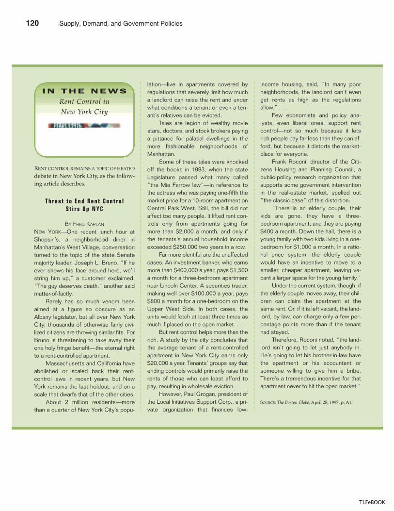
124 PART TWO SUPPLY AND DEMAND I : HOW MARKETS WORK
RENT CONTROL REMAINS A TOPIC OF HEATED
debate in New York City, as the follow-ing article describes.
T h r e a t t o E n d R e n t C o n t r o lS t i r s U p N Y C
BY FRED KAPLAN
NEW YORK—One recent lunch hour atShopsin’s, a neighborhood diner inManhattan’s West Village, conversationturned to the topic of the state Senatemajority leader, Joseph L. Bruno. “If heever shows his face around here, we’llstring him up,” a customer exclaimed.“The guy deserves death,” another saidmatter-of-factly.
Rarely has so much venom beenaimed at a figure so obscure as anAlbany legislator, but all over New YorkCity, thousands of otherwise fairly civi-lized citizens are throwing similar fits. ForBruno is threatening to take away theirone holy fringe benefit—the eternal rightto a rent-controlled apartment.
Massachusetts and California haveabolished or scaled back their rent-control laws in recent years, but NewYork remains the last holdout, and on ascale that dwarfs that of the other cities.
About 2 million residents—morethan a quarter of New York City’s popu-
lation—live in apartments covered byregulations that severely limit how mucha landlord can raise the rent and underwhat conditions a tenant or even a ten-ant’s relatives can be evicted.
Tales are legion of wealthy moviestars, doctors, and stock brokers payinga pittance for palatial dwellings in themore fashionable neighborhoods ofManhattan.
Some of these tales were knockedoff the books in 1993, when the stateLegislature passed what many called“the Mia Farrow law”—in reference tothe actress who was paying one-fifth themarket price for a 10-room apartment onCentral Park West. Still, the bill did notaffect too many people. It lifted rent con-trols only from apartments going formore than $2,000 a month, and only ifthe tenants’s annual household incomeexceeded $250,000 two years in a row.
Far more plentiful are the unaffectedcases. An investment banker, who earnsmore than $400,000 a year, pays $1,500a month for a three-bedroom apartmentnear Lincoln Center. A securities trader,making well over $100,000 a year, pays$800 a month for a one-bedroom on theUpper West Side. In both cases, theunits would fetch at least three times asmuch if placed on the open market. . . .
But rent control helps more than therich. A study by the city concludes thatthe average tenant of a rent-controlledapartment in New York City earns only$20,000 a year. Tenants’ groups say thatending controls would primarily raise therents of those who can least afford topay, resulting in wholesale eviction.
However, Paul Grogan, president ofthe Local Initiatives Support Corp., a pri-vate organization that finances low-
income housing, said, “In many poorneighborhoods, the landlord can’t evenget rents as high as the regulationsallow.” . . .
Few economists and policy ana-lysts, even liberal ones, support rentcontrol—not so much because it letsrich people pay far less than they can af-ford, but because it distorts the market-place for everyone.
Frank Roconi, director of the Citi-zens Housing and Planning Council, apublic-policy research organization thatsupports some government interventionin the real-estate market, spelled out“the classic case” of this distortion:
“There is an elderly couple, theirkids are gone, they have a three-bedroom apartment, and they are paying$400 a month. Down the hall, there is ayoung family with two kids living in a one-bedroom for $1,000 a month. In a ratio-nal price system, the elderly couplewould have an incentive to move to asmaller, cheaper apartment, leaving va-cant a larger space for the young family.”
Under the current system, though, ifthe elderly couple moves away, their chil-dren can claim the apartment at thesame rent. Or, if it is left vacant, the land-lord, by law, can charge only a few per-centage points more than if the tenanthad stayed.
Therefore, Roconi noted, “the land-lord isn’t going to let just anybody in.He’s going to let his brother-in-law havethe apartment or his accountant orsomeone willing to give him a bribe.There’s a tremendous incentive for thatapartment never to hit the open market.”
SOURCE: The Boston Globe, April 28, 1997, p. A1.
IN THE NEWS
Rent Control in New York City
120 Supply, Demand, and Government Policies
TLFeBOOK
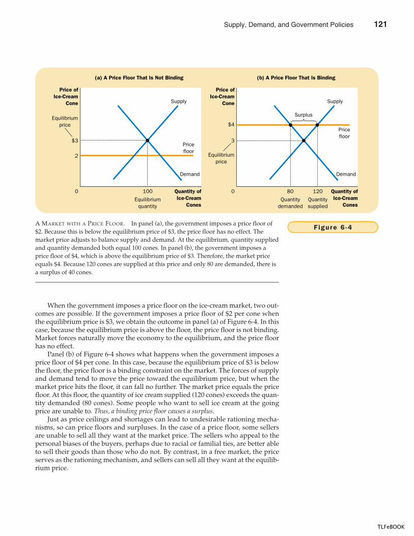
CHAPTER 6 SUPPLY, DEMAND, AND GOVERNMENT POLICIES 125
When the government imposes a price floor on the ice-cream market, two out-comes are possible. If the government imposes a price floor of $2 per cone whenthe equilibrium price is $3, we obtain the outcome in panel (a) of Figure 6-4. In thiscase, because the equilibrium price is above the floor, the price floor is not binding.Market forces naturally move the economy to the equilibrium, and the price floorhas no effect.
Panel (b) of Figure 6-4 shows what happens when the government imposes aprice floor of $4 per cone. In this case, because the equilibrium price of $3 is belowthe floor, the price floor is a binding constraint on the market. The forces of supplyand demand tend to move the price toward the equilibrium price, but when themarket price hits the floor, it can fall no further. The market price equals the pricefloor. At this floor, the quantity of ice cream supplied (120 cones) exceeds the quan-tity demanded (80 cones). Some people who want to sell ice cream at the goingprice are unable to. Thus, a binding price floor causes a surplus.
Just as price ceilings and shortages can lead to undesirable rationing mecha-nisms, so can price floors and surpluses. In the case of a price floor, some sellersare unable to sell all they want at the market price. The sellers who appeal to thepersonal biases of the buyers, perhaps due to racial or familial ties, are better ableto sell their goods than those who do not. By contrast, in a free market, the priceserves as the rationing mechanism, and sellers can sell all they want at the equilib-rium price.
(a) A Price Floor That Is Not Binding
$3
2
Quantity ofIce-Cream
Cones
0
Price ofIce-Cream
Cone
100
Equilibriumquantity
(b) A Price Floor That Is Binding
$4
Quantity ofIce-Cream
Cones
0
Price ofIce-Cream
Cone
3Pricefloor
Demand
Supply
Pricefloor
80
Quantitydemanded
120
Quantitysupplied
Equilibriumprice
Equilibriumprice
Demand
Supply
Surplus
Figure 6 -4A MARKET WITH A PRICE FLOOR. In panel (a), the government imposes a price floor of$2. Because this is below the equilibrium price of $3, the price floor has no effect. Themarket price adjusts to balance supply and demand. At the equilibrium, quantity suppliedand quantity demanded both equal 100 cones. In panel (b), the government imposes aprice floor of $4, which is above the equilibrium price of $3. Therefore, the market priceequals $4. Because 120 cones are supplied at this price and only 80 are demanded, there isa surplus of 40 cones.
Supply, Demand, and Government Policies 121
TLFeBOOK
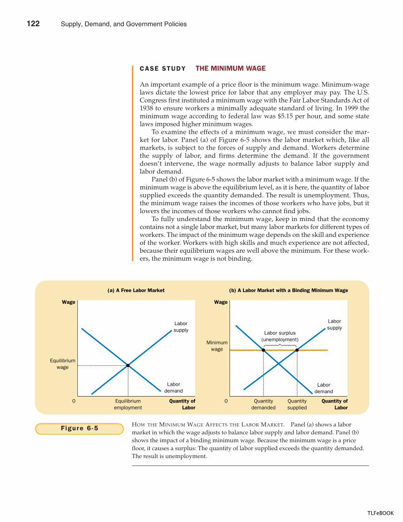
126 PART TWO SUPPLY AND DEMAND I : HOW MARKETS WORK
CASE STUDY THE MINIMUM WAGE
An important example of a price floor is the minimum wage. Minimum-wagelaws dictate the lowest price for labor that any employer may pay. The U.S.Congress first instituted a minimum wage with the Fair Labor Standards Act of1938 to ensure workers a minimally adequate standard of living. In 1999 theminimum wage according to federal law was $5.15 per hour, and some statelaws imposed higher minimum wages.
To examine the effects of a minimum wage, we must consider the mar-ket for labor. Panel (a) of Figure 6-5 shows the labor market which, like allmarkets, is subject to the forces of supply and demand. Workers determinethe supply of labor, and firms determine the demand. If the governmentdoesn’t intervene, the wage normally adjusts to balance labor supply andlabor demand.
Panel (b) of Figure 6-5 shows the labor market with a minimum wage. If theminimum wage is above the equilibrium level, as it is here, the quantity of laborsupplied exceeds the quantity demanded. The result is unemployment. Thus,the minimum wage raises the incomes of those workers who have jobs, but itlowers the incomes of those workers who cannot find jobs.
To fully understand the minimum wage, keep in mind that the economycontains not a single labor market, but many labor markets for different types ofworkers. The impact of the minimum wage depends on the skill and experienceof the worker. Workers with high skills and much experience are not affected,because their equilibrium wages are well above the minimum. For these work-ers, the minimum wage is not binding.
(a) A Free Labor Market
Quantity ofLabor
0
Wage
Equilibriumemployment
(b) A Labor Market with a Binding Minimum Wage
Quantity ofLabor
0
Wage
Quantitydemanded
Quantitysupplied
Laborsupply
Labordemand
Minimumwage
Labor surplus(unemployment)
Equilibriumwage
Labordemand
Laborsupply
Figure 6 -5 HOW THE MINIMUM WAGE AFFECTS THE LABOR MARKET. Panel (a) shows a labormarket in which the wage adjusts to balance labor supply and labor demand. Panel (b)shows the impact of a binding minimum wage. Because the minimum wage is a pricefloor, it causes a surplus: The quantity of labor supplied exceeds the quantity demanded.The result is unemployment.
122 Supply, Demand, and Government Policies
TLFeBOOK
CHAPTER 6 SUPPLY, DEMAND, AND GOVERNMENT POLICIES 127
The minimum wage has its greatest impact on the market for teenage labor.The equilibrium wages of teenagers are low because teenagers are among theleast skilled and least experienced members of the labor force. In addition,teenagers are often willing to accept a lower wage in exchange for on-the-jobtraining. (Some teenagers are willing to work as “interns” for no pay at all. Be-cause internships pay nothing, however, the minimum wage does not apply tothem. If it did, these jobs might not exist.) As a result, the minimum wage ismore often binding for teenagers than for other members of the labor force.
Many economists have studied how minimum-wage laws affect the teenagelabor market. These researchers compare the changes in the minimum wage overtime with the changes in teenage employment. Although there is some debateabout how much the minimum wage affects employment, the typical study findsthat a 10 percent increase in the minimum wage depresses teenage employmentbetween 1 and 3 percent. In interpreting this estimate, note that a 10 percent in-crease in the minimum wage does not raise the average wage of teenagers by 10percent. A change in the law does not directly affect those teenagers who are al-ready paid well above the minimum, and enforcement of minimum-wage laws isnot perfect. Thus, the estimated drop in employment of 1 to 3 percent is significant.
In addition to altering the quantity of labor demanded, the minimum wagealso alters the quantity supplied. Because the minimum wage raises the wagethat teenagers can earn, it increases the number of teenagers who choose to lookfor jobs. Studies have found that a higher minimum wage influences whichteenagers are employed. When the minimum wage rises, some teenagers whoare still attending school choose to drop out and take jobs. These new dropoutsdisplace other teenagers who had already dropped out of school and who nowbecome unemployed.
The minimum wage is a frequent topic of political debate. Advocates of theminimum wage view the policy as one way to raise the income of the workingpoor. They correctly point out that workers who earn the minimum wage canafford only a meager standard of living. In 1999, for instance, when the mini-mum wage was $5.15 per hour, two adults working 40 hours a week for everyweek of the year at minimum-wage jobs had a total annual income of only$21,424, which was less than half of the median family income. Many advocatesof the minimum wage admit that it has some adverse effects, including unem-ployment, but they believe that these effects are small and that, all things con-sidered, a higher minimum wage makes the poor better off.
Opponents of the minimum wage contend that it is not the best way tocombat poverty. They note that a high minimum wage causes unemployment,encourages teenagers to drop out of school, and prevents some unskilled work-ers from getting the on-the-job training they need. Moreover, opponents of theminimum wage point out that the minimum wage is a poorly targeted policy.Not all minimum-wage workers are heads of households trying to help theirfamilies escape poverty. In fact, fewer than a third of minimum-wage earnersare in families with incomes below the poverty line. Many are teenagers frommiddle-class homes working at part-time jobs for extra spending money.
EVALUATING PRICE CONTROLS
One of the Ten Principles of Economics discussed in Chapter 1 is that markets areusually a good way to organize economic activity. This principle explains why
Supply, Demand, and Government Policies 123
TLFeBOOK
128 PART TWO SUPPLY AND DEMAND I : HOW MARKETS WORK
economists usually oppose price ceilings and price floors. To economists, prices arenot the outcome of some haphazard process. Prices, they contend, are the result of themillions of business and consumer decisions that lie behind the supply and demandcurves. Prices have the crucial job of balancing supply and demand and, thereby, co-ordinating economic activity. When policymakers set prices by legal decree, they ob-scure the signals that normally guide the allocation of society’s resources.
Another one of the Ten Principles of Economics is that governments can some-times improve market outcomes. Indeed, policymakers are led to control prices be-cause they view the market’s outcome as unfair. Price controls are often aimed athelping the poor. For instance, rent-control laws try to make housing affordable foreveryone, and minimum-wage laws try to help people escape poverty.
Yet price controls often hurt those they are trying to help. Rent control maykeep rents low, but it also discourages landlords from maintaining their buildingsand makes housing hard to find. Minimum-wage laws may raise the incomes ofsome workers, but they also cause other workers to be unemployed.
Helping those in need can be accomplished in ways other than controlling prices.For instance, the government can make housing more affordable by paying a fractionof the rent for poor families. Unlike rent control, such rent subsidies do not reduce thequantity of housing supplied and, therefore, do not lead to housing shortages. Simi-larly, wage subsidies raise the living standards of the working poor without discour-aging firms from hiring them. An example of a wage subsidy is the earned income taxcredit, a government program that supplements the incomes of low-wage workers.
Although these alternative policies are often better than price controls, they arenot perfect. Rent and wage subsidies cost the government money and, therefore,require higher taxes. As we see in the next section, taxation has costs of its own.
QUICK QUIZ: Define price ceiling and price floor, and give an example of each. Which leads to a shortage? Which leads to a surplus? Why?
TAXES
All governments—from the federal government in Washington, D.C., to the localgovernments in small towns—use taxes to raise revenue for public projects, suchas roads, schools, and national defense. Because taxes are such an important pol-icy instrument, and because they affect our lives in many ways, the study of taxesis a topic to which we return several times throughout this book. In this section webegin our study of how taxes affect the economy.
To set the stage for our analysis, imagine that a local government decides tohold an annual ice-cream celebration—with a parade, fireworks, and speeches bytown officials. To raise revenue to pay for the event, it decides to place a $0.50 taxon the sale of ice-cream cones. When the plan is announced, our two lobbyinggroups swing into action. The National Organization of Ice Cream Makers claimsthat its members are struggling to survive in a competitive market, and it arguesthat buyers of ice cream should have to pay the tax. The American Association ofIce Cream Eaters claims that consumers of ice cream are having trouble makingends meet, and it argues that sellers of ice cream should pay the tax. The townmayor, hoping to reach a compromise, suggests that half the tax be paid by thebuyers and half be paid by the sellers.
124 Supply, Demand, and Government Policies
TLFeBOOK
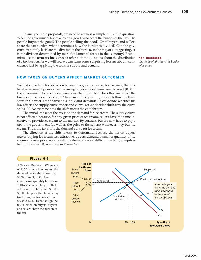
CHAPTER 6 SUPPLY, DEMAND, AND GOVERNMENT POLICIES 129
To analyze these proposals, we need to address a simple but subtle question:When the government levies a tax on a good, who bears the burden of the tax? Thepeople buying the good? The people selling the good? Or, if buyers and sellersshare the tax burden, what determines how the burden is divided? Can the gov-ernment simply legislate the division of the burden, as the mayor is suggesting, oris the division determined by more fundamental forces in the economy? Econo-mists use the term tax incidence to refer to these questions about the distributionof a tax burden. As we will see, we can learn some surprising lessons about tax in-cidence just by applying the tools of supply and demand.
HOW TAXES ON BUYERS AFFECT MARKET OUTCOMES
We first consider a tax levied on buyers of a good. Suppose, for instance, that ourlocal government passes a law requiring buyers of ice-cream cones to send $0.50 tothe government for each ice-cream cone they buy. How does this law affect thebuyers and sellers of ice cream? To answer this question, we can follow the threesteps in Chapter 4 for analyzing supply and demand: (1) We decide whether thelaw affects the supply curve or demand curve. (2) We decide which way the curveshifts. (3) We examine how the shift affects the equilibrium.
The initial impact of the tax is on the demand for ice cream. The supply curveis not affected because, for any given price of ice cream, sellers have the same in-centive to provide ice cream to the market. By contrast, buyers now have to pay atax to the government (as well as the price to the sellers) whenever they buy icecream. Thus, the tax shifts the demand curve for ice cream.
The direction of the shift is easy to determine. Because the tax on buyersmakes buying ice cream less attractive, buyers demand a smaller quantity of icecream at every price. As a result, the demand curve shifts to the left (or, equiva-lently, downward), as shown in Figure 6-6.
tax inc idencethe study of who bears the burdenof taxation
$3.303.002.80
Quantity ofIce-Cream Cones
0
Price ofIce-Cream
Cone
Pricewithout
tax
Pricesellersreceive
10090
Equilibriumwith tax
Equilibrium without taxTax ($0.50)
Pricebuyers
pay
D1
D2
Supply, S1
A tax on buyersshifts the demandcurve downwardby the size ofthe tax ($0.50).
Figure 6 -6
A TAX ON BUYERS. When a taxof $0.50 is levied on buyers, thedemand curve shifts down by$0.50 from D1 to D2. Theequilibrium quantity falls from100 to 90 cones. The price thatsellers receive falls from $3.00 to$2.80. The price that buyers pay(including the tax) rises from$3.00 to $3.30. Even though thetax is levied on buyers, buyersand sellers share the burden ofthe tax.
Supply, Demand, and Government Policies 125
TLFeBOOK
130 PART TWO SUPPLY AND DEMAND I : HOW MARKETS WORK
We can, in this case, be precise about how much the curve shifts. Because ofthe $0.50 tax levied on buyers, the effective price to buyers is now $0.50 higherthan the market price. For example, if the market price of a cone happened to be$2.00, the effective price to buyers would be $2.50. Because buyers look at their to-tal cost including the tax, they demand a quantity of ice cream as if the marketprice were $0.50 higher than it actually is. In other words, to induce buyers to de-mand any given quantity, the market price must now be $0.50 lower to make upfor the effect of the tax. Thus, the tax shifts the demand curve downward from D1 toD2 by exactly the size of the tax ($0.50).
To see the effect of the tax, we compare the old equilibrium and the new equi-librium. You can see in the figure that the equilibrium price of ice cream falls from$3.00 to $2.80 and the equilibrium quantity falls from 100 to 90 cones. Because sell-ers sell less and buyers buy less in the new equilibrium, the tax on ice cream re-duces the size of the ice-cream market.
Now let’s return to the question of tax incidence: Who pays the tax? Althoughbuyers send the entire tax to the government, buyers and sellers share the burden.Because the market price falls from $3.00 to $2.80 when the tax is introduced, sellersreceive $0.20 less for each ice-cream cone than they did without the tax. Thus, thetax makes sellers worse off. Buyers pay sellers a lower price ($2.80), but the effectiveprice including the tax rises from $3.00 before the tax to $3.30 with the tax ($2.80 +$0.50 = $3.30). Thus, the tax also makes buyers worse off.
To sum up, the analysis yields two general lessons:
� Taxes discourage market activity. When a good is taxed, the quantity of thegood sold is smaller in the new equilibrium.
� Buyers and sellers share the burden of taxes. In the new equilibrium, buyerspay more for the good, and sellers receive less.
HOW TAXES ON SELLERS AFFECT MARKET OUTCOMES
Now consider a tax levied on sellers of a good. Suppose the local governmentpasses a law requiring sellers of ice-cream cones to send $0.50 to the governmentfor each cone they sell. What are the effects of this law?
In this case, the initial impact of the tax is on the supply of ice cream. Becausethe tax is not levied on buyers, the quantity of ice cream demanded at any givenprice is the same, so the demand curve does not change. By contrast, the tax on sell-ers raises the cost of selling ice cream, and leads sellers to supply a smaller quantityat every price. The supply curve shifts to the left (or, equivalently, upward).
Once again, we can be precise about the magnitude of the shift. For any mar-ket price of ice cream, the effective price to sellers—the amount they get to keep af-ter paying the tax—is $0.50 lower. For example, if the market price of a conehappened to be $2.00, the effective price received by sellers would be $1.50. What-ever the market price, sellers will supply a quantity of ice cream as if the pricewere $0.50 lower than it is. Put differently, to induce sellers to supply any givenquantity, the market price must now be $0.50 higher to compensate for the effect ofthe tax. Thus, as shown in Figure 6-7, the supply curve shifts upward from S1 to S2
by exactly the size of the tax ($0.50).When the market moves from the old to the new equilibrium, the equilibrium
price of ice cream rises from $3.00 to $3.30, and the equilibrium quantity falls from
126 Supply, Demand, and Government Policies
TLFeBOOK
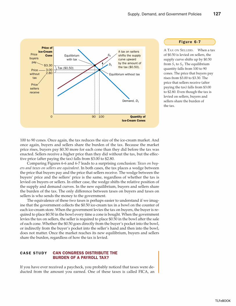
CHAPTER 6 SUPPLY, DEMAND, AND GOVERNMENT POLICIES 131
CASE STUDY CAN CONGRESS DISTRIBUTE THEBURDEN OF A PAYROLL TAX?
If you have ever received a paycheck, you probably noticed that taxes were de-ducted from the amount you earned. One of these taxes is called FICA, an
100 to 90 cones. Once again, the tax reduces the size of the ice-cream market. Andonce again, buyers and sellers share the burden of the tax. Because the marketprice rises, buyers pay $0.30 more for each cone than they did before the tax wasenacted. Sellers receive a higher price than they did without the tax, but the effec-tive price (after paying the tax) falls from $3.00 to $2.80.
Comparing Figures 6-6 and 6-7 leads to a surprising conclusion: Taxes on buy-ers and taxes on sellers are equivalent. In both cases, the tax places a wedge betweenthe price that buyers pay and the price that sellers receive. The wedge between thebuyers’ price and the sellers’ price is the same, regardless of whether the tax islevied on buyers or sellers. In either case, the wedge shifts the relative position ofthe supply and demand curves. In the new equilibrium, buyers and sellers sharethe burden of the tax. The only difference between taxes on buyers and taxes onsellers is who sends the money to the government.
The equivalence of these two taxes is perhaps easier to understand if we imag-ine that the government collects the $0.50 ice-cream tax in a bowl on the counter ofeach ice-cream store. When the government levies the tax on buyers, the buyer is re-quired to place $0.50 in the bowl every time a cone is bought. When the governmentlevies the tax on sellers, the seller is required to place $0.50 in the bowl after the saleof each cone. Whether the $0.50 goes directly from the buyer’s pocket into the bowl,or indirectly from the buyer’s pocket into the seller’s hand and then into the bowl,does not matter. Once the market reaches its new equilibrium, buyers and sellersshare the burden, regardless of how the tax is levied.
$3.303.002.80
Quantity ofIce-Cream Cones
0
Price ofIce-Cream
Cone
Pricewithout
tax
Pricesellersreceive
10090
Equilibriumwith tax
Equilibrium without tax
Tax ($0.50)
Pricebuyers
payS1
S2
Demand, D1
A tax on sellersshifts the supplycurve upwardby the amount ofthe tax ($0.50).
Figure 6 -7
A TAX ON SELLERS. When a taxof $0.50 is levied on sellers, thesupply curve shifts up by $0.50from S1 to S2. The equilibriumquantity falls from 100 to 90cones. The price that buyers payrises from $3.00 to $3.30. Theprice that sellers receive (afterpaying the tax) falls from $3.00to $2.80. Even though the tax islevied on sellers, buyers andsellers share the burden ofthe tax.
Supply, Demand, and Government Policies 127
TLFeBOOK
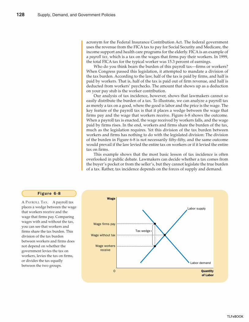
132 PART TWO SUPPLY AND DEMAND I : HOW MARKETS WORK
acronym for the Federal Insurance Contribution Act. The federal governmentuses the revenue from the FICA tax to pay for Social Security and Medicare, theincome support and health care programs for the elderly. FICA is an example ofa payroll tax, which is a tax on the wages that firms pay their workers. In 1999,the total FICA tax for the typical worker was 15.3 percent of earnings.
Who do you think bears the burden of this payroll tax—firms or workers?When Congress passed this legislation, it attempted to mandate a division ofthe tax burden. According to the law, half of the tax is paid by firms, and half ispaid by workers. That is, half of the tax is paid out of firm revenue, and half isdeducted from workers’ paychecks. The amount that shows up as a deductionon your pay stub is the worker contribution.
Our analysis of tax incidence, however, shows that lawmakers cannot soeasily distribute the burden of a tax. To illustrate, we can analyze a payroll taxas merely a tax on a good, where the good is labor and the price is the wage. Thekey feature of the payroll tax is that it places a wedge between the wage thatfirms pay and the wage that workers receive. Figure 6-8 shows the outcome.When a payroll tax is enacted, the wage received by workers falls, and the wagepaid by firms rises. In the end, workers and firms share the burden of the tax,much as the legislation requires. Yet this division of the tax burden betweenworkers and firms has nothing to do with the legislated division: The divisionof the burden in Figure 6-8 is not necessarily fifty-fifty, and the same outcomewould prevail if the law levied the entire tax on workers or if it levied the entiretax on firms.
This example shows that the most basic lesson of tax incidence is oftenoverlooked in public debate. Lawmakers can decide whether a tax comes fromthe buyer’s pocket or from the seller’s, but they cannot legislate the true burdenof a tax. Rather, tax incidence depends on the forces of supply and demand.
Wage without tax
Quantityof Labor
0
Wage
Labor demand
Labor supply
Tax wedge
Wage workersreceive
Wage firms pay
Figure 6 -8
A PAYROLL TAX. A payroll taxplaces a wedge between the wagethat workers receive and thewage that firms pay. Comparingwages with and without the tax,you can see that workers andfirms share the tax burden. Thisdivision of the tax burdenbetween workers and firms doesnot depend on whether thegovernment levies the tax onworkers, levies the tax on firms,or divides the tax equallybetween the two groups.
128 Supply, Demand, and Government Policies
TLFeBOOK
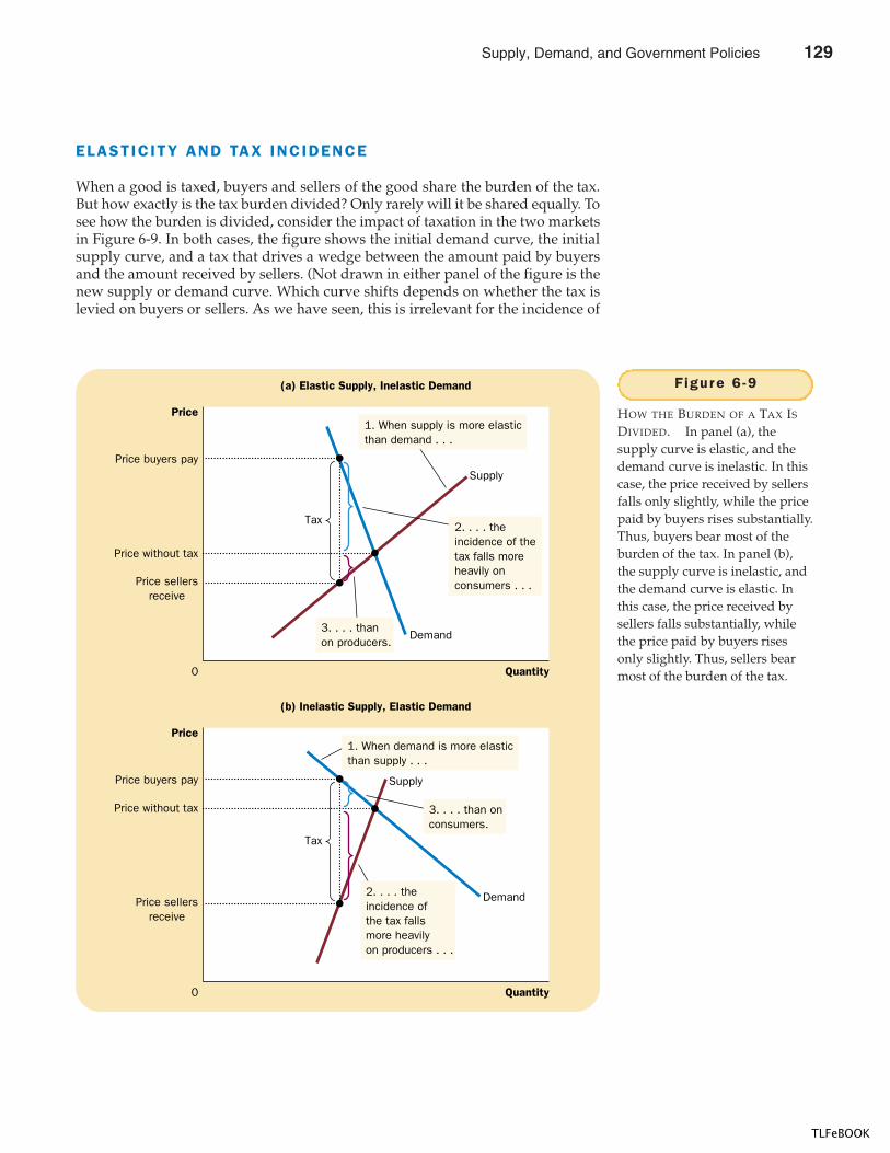
CHAPTER 6 SUPPLY, DEMAND, AND GOVERNMENT POLICIES 133
ELASTICITY AND TAX INCIDENCE
When a good is taxed, buyers and sellers of the good share the burden of the tax.But how exactly is the tax burden divided? Only rarely will it be shared equally. Tosee how the burden is divided, consider the impact of taxation in the two marketsin Figure 6-9. In both cases, the figure shows the initial demand curve, the initialsupply curve, and a tax that drives a wedge between the amount paid by buyersand the amount received by sellers. (Not drawn in either panel of the figure is thenew supply or demand curve. Which curve shifts depends on whether the tax islevied on buyers or sellers. As we have seen, this is irrelevant for the incidence of
Price without tax
Quantity0
Price
Demand
Supply
Tax
Price sellersreceive
Price buyers pay
(a) Elastic Supply, Inelastic Demand
Price without tax
Quantity0
Price
Demand
Supply
Tax
Price sellersreceive
Price buyers pay
(b) Inelastic Supply, Elastic Demand
2. . . . theincidence of thetax falls moreheavily onconsumers . . .
1. When supply is more elasticthan demand . . .
3. . . . than on producers.
2. . . . theincidence of the tax falls more heavily on producers . . .
3. . . . than onconsumers.
1. When demand is more elasticthan supply . . .
Figure 6 -9
HOW THE BURDEN OF A TAX IS
DIVIDED. In panel (a), thesupply curve is elastic, and thedemand curve is inelastic. In thiscase, the price received by sellersfalls only slightly, while the pricepaid by buyers rises substantially.Thus, buyers bear most of theburden of the tax. In panel (b),the supply curve is inelastic, andthe demand curve is elastic. Inthis case, the price received bysellers falls substantially, whilethe price paid by buyers risesonly slightly. Thus, sellers bearmost of the burden of the tax.
Supply, Demand, and Government Policies 129
TLFeBOOK
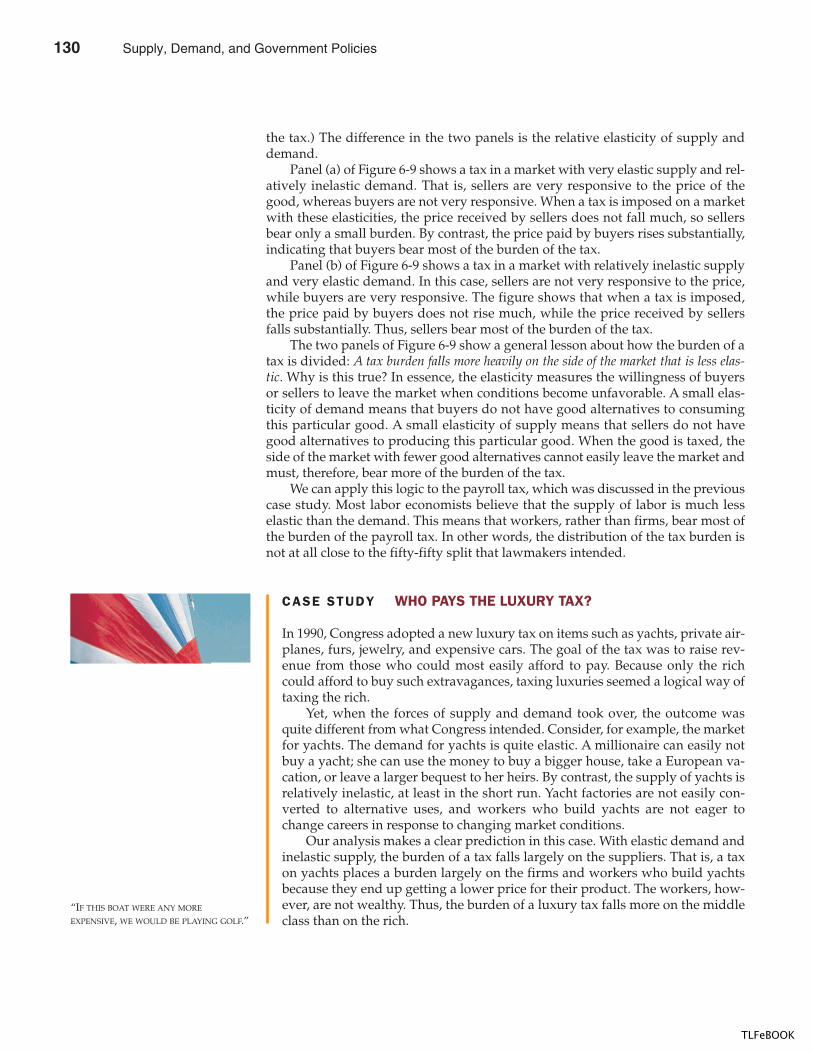
134 PART TWO SUPPLY AND DEMAND I : HOW MARKETS WORK
CASE STUDY WHO PAYS THE LUXURY TAX?
In 1990, Congress adopted a new luxury tax on items such as yachts, private air-planes, furs, jewelry, and expensive cars. The goal of the tax was to raise rev-enue from those who could most easily afford to pay. Because only the richcould afford to buy such extravagances, taxing luxuries seemed a logical way oftaxing the rich.
Yet, when the forces of supply and demand took over, the outcome wasquite different from what Congress intended. Consider, for example, the marketfor yachts. The demand for yachts is quite elastic. A millionaire can easily notbuy a yacht; she can use the money to buy a bigger house, take a European va-cation, or leave a larger bequest to her heirs. By contrast, the supply of yachts isrelatively inelastic, at least in the short run. Yacht factories are not easily con-verted to alternative uses, and workers who build yachts are not eager tochange careers in response to changing market conditions.
Our analysis makes a clear prediction in this case. With elastic demand andinelastic supply, the burden of a tax falls largely on the suppliers. That is, a taxon yachts places a burden largely on the firms and workers who build yachtsbecause they end up getting a lower price for their product. The workers, how-ever, are not wealthy. Thus, the burden of a luxury tax falls more on the middleclass than on the rich.
the tax.) The difference in the two panels is the relative elasticity of supply anddemand.
Panel (a) of Figure 6-9 shows a tax in a market with very elastic supply and rel-atively inelastic demand. That is, sellers are very responsive to the price of thegood, whereas buyers are not very responsive. When a tax is imposed on a marketwith these elasticities, the price received by sellers does not fall much, so sellersbear only a small burden. By contrast, the price paid by buyers rises substantially,indicating that buyers bear most of the burden of the tax.
Panel (b) of Figure 6-9 shows a tax in a market with relatively inelastic supplyand very elastic demand. In this case, sellers are not very responsive to the price,while buyers are very responsive. The figure shows that when a tax is imposed,the price paid by buyers does not rise much, while the price received by sellersfalls substantially. Thus, sellers bear most of the burden of the tax.
The two panels of Figure 6-9 show a general lesson about how the burden of atax is divided: A tax burden falls more heavily on the side of the market that is less elas-tic. Why is this true? In essence, the elasticity measures the willingness of buyersor sellers to leave the market when conditions become unfavorable. A small elas-ticity of demand means that buyers do not have good alternatives to consumingthis particular good. A small elasticity of supply means that sellers do not havegood alternatives to producing this particular good. When the good is taxed, theside of the market with fewer good alternatives cannot easily leave the market andmust, therefore, bear more of the burden of the tax.
We can apply this logic to the payroll tax, which was discussed in the previouscase study. Most labor economists believe that the supply of labor is much lesselastic than the demand. This means that workers, rather than firms, bear most ofthe burden of the payroll tax. In other words, the distribution of the tax burden isnot at all close to the fifty-fifty split that lawmakers intended.
“IF THIS BOAT WERE ANY MORE
EXPENSIVE, WE WOULD BE PLAYING GOLF.”
130 Supply, Demand, and Government Policies
TLFeBOOK
CHAPTER 6 SUPPLY, DEMAND, AND GOVERNMENT POLICIES 135
The mistaken assumptions about the incidence of the luxury tax quickly be-came apparent after the tax went into effect. Suppliers of luxuries made theircongressional representatives well aware of the economic hardship they experi-enced, and Congress repealed most of the luxury tax in 1993.
QUICK QUIZ: In a supply-and-demand diagram, show how a tax on car buyers of $1,000 per car affects the quantity of cars sold and the price of cars. In another diagram, show how a tax on car sellers of $1,000 per car affects thequantity of cars sold and the price of cars. In both of your diagrams, show thechange in the price paid by car buyers and the change in price received by car sellers.
CONCLUSION
The economy is governed by two kinds of laws: the laws of supply and demandand the laws enacted by governments. In this chapter we have begun to see howthese laws interact. Price controls and taxes are common in various markets in theeconomy, and their effects are frequently debated in the press and among policy-makers. Even a little bit of economic knowledge can go a long way toward under-standing and evaluating these policies.
In subsequent chapters we will analyze many government policies in greaterdetail. We will examine the effects of taxation more fully, and we will consider abroader range of policies than we considered here. Yet the basic lessons of thischapter will not change: When analyzing government policies, supply and de-mand are the first and most useful tools of analysis.
� A price ceiling is a legal maximum on the price of agood or service. An example is rent control. If the priceceiling is below the equilibrium price, the quantitydemanded exceeds the quantity supplied. Because ofthe resulting shortage, sellers must in some way rationthe good or service among buyers.
� A price floor is a legal minimum on the price of a goodor service. An example is the minimum wage. If theprice floor is above the equilibrium price, the quantitysupplied exceeds the quantity demanded. Because ofthe resulting surplus, buyers’ demands for the good orservice must in some way be rationed among sellers.
� When the government levies a tax on a good, theequilibrium quantity of the good falls. That is, a tax on amarket shrinks the size of the market.
� A tax on a good places a wedge between the price paidby buyers and the price received by sellers. When themarket moves to the new equilibrium, buyers pay morefor the good and sellers receive less for it. In this sense,buyers and sellers share the tax burden. The incidenceof a tax does not depend on whether the tax is levied onbuyers or sellers.
� The incidence of a tax depends on the price elasticitiesof supply and demand. The burden tends to fall on theside of the market that is less elastic because that side ofthe market can respond less easily to the tax bychanging the quantity bought or sold.
Summar y
Supply, Demand, and Government Policies 131
TLFeBOOK
136 PART TWO SUPPLY AND DEMAND I : HOW MARKETS WORK
price ceiling, p. 118 price floor, p. 118 tax incidence, p. 129
Key Concepts
1. Give an example of a price ceiling and an example of aprice floor.
2. Which causes a shortage of a good—a price ceiling or aprice floor? Which causes a surplus?
3. What mechanisms allocate resources when the price of agood is not allowed to bring supply and demand intoequilibrium?
4. Explain why economists usually oppose controls onprices.
5. What is the difference between a tax paid by buyers anda tax paid by sellers?
6. How does a tax on a good affect the price paid bybuyers, the price received by sellers, and the quantitysold?
7. What determines how the burden of a tax is dividedbetween buyers and sellers? Why?
Quest ions fo r Rev iew
1. Lovers of classical music persuade Congress to impose aprice ceiling of $40 per ticket. Does this policy get moreor fewer people to attend classical music concerts?
2. The government has decided that the free-market priceof cheese is too low.a. Suppose the government imposes a binding price
floor in the cheese market. Use a supply-and-demand diagram to show the effect of this policyon the price of cheese and the quantity of cheesesold. Is there a shortage or surplus of cheese?
b. Farmers complain that the price floor has reducedtheir total revenue. Is this possible? Explain.
c. In response to farmers’ complaints, the governmentagrees to purchase all of the surplus cheese at theprice floor. Compared to the basic price floor, whobenefits from this new policy? Who loses?
3. A recent study found that the demand and supplyschedules for Frisbees are as follows:
PRICE PER QUANTITY QUANTITY
FRISBEE DEMANDED SUPPLIED
$11 1 million 15 million10 2 129 4 98 6 67 8 36 10 1
a. What are the equilibrium price and quantity ofFrisbees?
b. Frisbee manufacturers persuade the governmentthat Frisbee production improves scientists’understanding of aerodynamics and thus isimportant for national security. A concernedCongress votes to impose a price floor $2 above theequilibrium price. What is the new market price?How many Frisbees are sold?
c. Irate college students march on Washington anddemand a reduction in the price of Frisbees. Aneven more concerned Congress votes to repeal theprice floor and impose a price ceiling $1 below theformer price floor. What is the new market price?How many Frisbees are sold?
4. Suppose the federal government requires beer drinkersto pay a $2 tax on each case of beer purchased. (In fact,both the federal and state governments impose beertaxes of some sort.)a. Draw a supply-and-demand diagram of the market
for beer without the tax. Show the price paid byconsumers, the price received by producers, andthe quantity of beer sold. What is the differencebetween the price paid by consumers and the pricereceived by producers?
b. Now draw a supply-and-demand diagram for thebeer market with the tax. Show the price paid byconsumers, the price received by producers, and
Prob lems and App l icat ions
132 Supply, Demand, and Government Policies
TLFeBOOK
CHAPTER 6 SUPPLY, DEMAND, AND GOVERNMENT POLICIES 137
the quantity of beer sold. What is the differencebetween the price paid by consumers and the pricereceived by producers? Has the quantity of beersold increased or decreased?
5. A senator wants to raise tax revenue and make workersbetter off. A staff member proposes raising the payrolltax paid by firms and using part of the extra revenue toreduce the payroll tax paid by workers. Would thisaccomplish the senator’s goal?
6. If the government places a $500 tax on luxury cars, willthe price paid by consumers rise by more than $500, lessthan $500, or exactly $500? Explain.
7. Congress and the president decide that the UnitedStates should reduce air pollution by reducing its use ofgasoline. They impose a $0.50 tax for each gallon ofgasoline sold.a. Should they impose this tax on producers or
consumers? Explain carefully using a supply-and-demand diagram.
b. If the demand for gasoline were more elastic,would this tax be more effective or less effective inreducing the quantity of gasoline consumed?Explain with both words and a diagram.
c. Are consumers of gasoline helped or hurt by thistax? Why?
d. Are workers in the oil industry helped or hurt bythis tax? Why?
8. A case study in this chapter discusses the federalminimum-wage law.a. Suppose the minimum wage is above the
equilibrium wage in the market for unskilled labor.Using a supply-and-demand diagram of the marketfor unskilled labor, show the market wage, thenumber of workers who are employed, and thenumber of workers who are unemployed. Alsoshow the total wage payments to unskilledworkers.
b. Now suppose the secretary of labor proposes anincrease in the minimum wage. What effect wouldthis increase have on employment? Does thechange in employment depend on the elasticity ofdemand, the elasticity of supply, both elasticities, orneither?
c. What effect would this increase in the minimumwage have on unemployment? Does the change inunemployment depend on the elasticity of demand,the elasticity of supply, both elasticities, or neither?
d. If the demand for unskilled labor were inelastic,would the proposed increase in the minimum wageraise or lower total wage payments to unskilledworkers? Would your answer change if the demandfor unskilled labor were elastic?
9. Consider the following policies, each of which is aimedat reducing violent crime by reducing the use of guns.Illustrate each of these proposed policies in a supply-and-demand diagram of the gun market.a. a tax on gun buyersb. a tax on gun sellersc. a price floor on gunsd. a tax on ammunition
10. The U.S. government administers two programs thataffect the market for cigarettes. Media campaigns andlabeling requirements are aimed at making the publicaware of the dangers of cigarette smoking. At the sametime, the Department of Agriculture maintains a pricesupport program for tobacco farmers, which raises theprice of tobacco above the equilibrium price.a. How do these two programs affect cigarette
consumption? Use a graph of the cigarette marketin your answer.
b. What is the combined effect of these two programson the price of cigarettes?
c. Cigarettes are also heavily taxed. What effect doesthis tax have on cigarette consumption?
11. A subsidy is the opposite of a tax. With a $0.50 tax onthe buyers of ice-cream cones, the government collects$0.50 for each cone purchased; with a $0.50 subsidy forthe buyers of ice-cream cones, the government paysbuyers $0.50 for each cone purchased.a. Show the effect of a $0.50 per cone subsidy on the
demand curve for ice-cream cones, the effectiveprice paid by consumers, the effective pricereceived by sellers, and the quantity of cones sold.
b. Do consumers gain or lose from this policy? Doproducers gain or lose? Does the government gainor lose?
Supply, Demand, and Government Policies 133
TLFeBOOK

TLFeBOOK
IN THIS CHAPTERYOU WILL . . .
See that theequ i l ib r ium of
supp ly and demandmaximizes tota l
surp lus in a market
Examine the l inkbetween se l le rs ’
costs o f p roduc inga good and the
supp ly cur ve
Examine the l inkbetween buyers ’
wi l l ingness to payfor a good and the
demand cur ve
Learn how to def ineand measure
consumer surp lus
Learn how to def ineand measure
producer surp lusWhen consumers go to grocery stores to buy their turkeys for Thanksgiving din-ner, they may be disappointed that the price of turkey is as high as it is. At thesame time, when farmers bring to market the turkeys they have raised, they wishthe price of turkey were even higher. These views are not surprising: Buyers al-ways want to pay less, and sellers always want to get paid more. But is there a“right price” for turkey from the standpoint of society as a whole?
In previous chapters we saw how, in market economies, the forces of supplyand demand determine the prices of goods and services and the quantities sold. Sofar, however, we have described the way markets allocate scarce resources withoutdirectly addressing the question of whether these market allocations are desirable.In other words, our analysis has been positive (what is) rather than normative (what
C O N S U M E R S , P R O D U C E R S ,
A N D T H E E F F I C I E N C Y
O F M A R K E T S
141
135
7
TLFeBOOK
142 PART THREE SUPPLY AND DEMAND I I : MARKETS AND WELFARE
should be). We know that the price of turkey adjusts to ensure that the quantity ofturkey supplied equals the quantity of turkey demanded. But, at this equilibrium,is the quantity of turkey produced and consumed too small, too large, or justright?
In this chapter we take up the topic of welfare economics, the study of howthe allocation of resources affects economic well-being. We begin by examining thebenefits that buyers and sellers receive from taking part in a market. We then ex-amine how society can make these benefits as large as possible. This analysis leadsto a profound conclusion: The equilibrium of supply and demand in a marketmaximizes the total benefits received by buyers and sellers.
As you may recall from Chapter 1, one of the Ten Principles of Economics is thatmarkets are usually a good way to organize economic activity. The study of wel-fare economics explains this principle more fully. It also answers our questionabout the right price of turkey: The price that balances the supply and demand forturkey is, in a particular sense, the best one because it maximizes the total welfareof turkey consumers and turkey producers.
CONSUMER SURPLUS
We begin our study of welfare economics by looking at the benefits buyers receivefrom participating in a market.
WILLINGNESS TO PAY
Imagine that you own a mint-condition recording of Elvis Presley’s first album.Because you are not an Elvis Presley fan, you decide to sell it. One way to do so isto hold an auction.
Four Elvis fans show up for your auction: John, Paul, George, and Ringo. Eachof them would like to own the album, but there is a limit to the amount that eachis willing to pay for it. Table 7-1 shows the maximum price that each of the fourpossible buyers would pay. Each buyer’s maximum is called his willingness topay, and it measures how much that buyer values the good. Each buyer would beeager to buy the album at a price less than his willingness to pay, would refuse to
wel fa re economicsthe study of how the allocation ofresources affects economic well-being
wi l l ingness to paythe maximum amount that a buyerwill pay for a good
Table 7 -1
FOUR POSSIBLE BUYERS’WILLINGNESS TO PAY
BUYER WILLINGNESS TO PAY
John $100Paul 80George 70Ringo 50
136 Consumers, Producers, and the Efficiency of Markets
TLFeBOOK
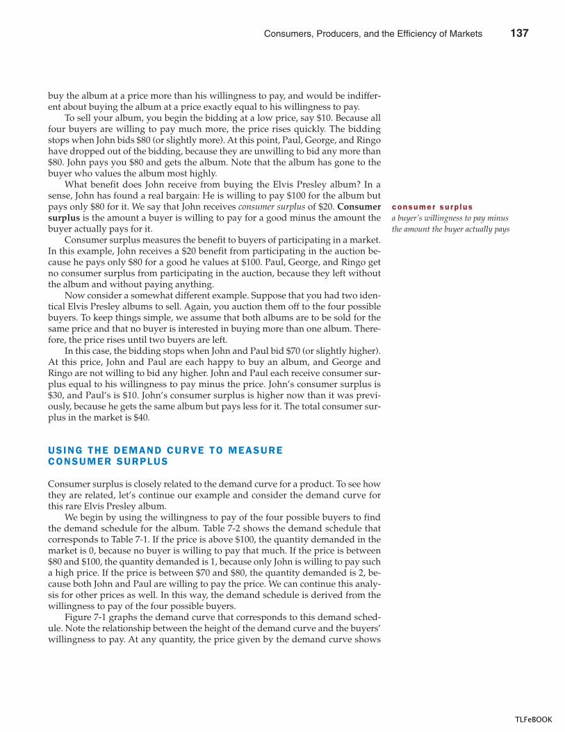
CHAPTER 7 CONSUMERS, PRODUCERS, AND THE EFFICIENCY OF MARKETS 143
buy the album at a price more than his willingness to pay, and would be indiffer-ent about buying the album at a price exactly equal to his willingness to pay.
To sell your album, you begin the bidding at a low price, say $10. Because allfour buyers are willing to pay much more, the price rises quickly. The biddingstops when John bids $80 (or slightly more). At this point, Paul, George, and Ringohave dropped out of the bidding, because they are unwilling to bid any more than$80. John pays you $80 and gets the album. Note that the album has gone to thebuyer who values the album most highly.
What benefit does John receive from buying the Elvis Presley album? In asense, John has found a real bargain: He is willing to pay $100 for the album butpays only $80 for it. We say that John receives consumer surplus of $20. Consumersurplus is the amount a buyer is willing to pay for a good minus the amount thebuyer actually pays for it.
Consumer surplus measures the benefit to buyers of participating in a market.In this example, John receives a $20 benefit from participating in the auction be-cause he pays only $80 for a good he values at $100. Paul, George, and Ringo getno consumer surplus from participating in the auction, because they left withoutthe album and without paying anything.
Now consider a somewhat different example. Suppose that you had two iden-tical Elvis Presley albums to sell. Again, you auction them off to the four possiblebuyers. To keep things simple, we assume that both albums are to be sold for thesame price and that no buyer is interested in buying more than one album. There-fore, the price rises until two buyers are left.
In this case, the bidding stops when John and Paul bid $70 (or slightly higher).At this price, John and Paul are each happy to buy an album, and George andRingo are not willing to bid any higher. John and Paul each receive consumer sur-plus equal to his willingness to pay minus the price. John’s consumer surplus is$30, and Paul’s is $10. John’s consumer surplus is higher now than it was previ-ously, because he gets the same album but pays less for it. The total consumer sur-plus in the market is $40.
USING THE DEMAND CURVE TO MEASURECONSUMER SURPLUS
Consumer surplus is closely related to the demand curve for a product. To see howthey are related, let’s continue our example and consider the demand curve forthis rare Elvis Presley album.
We begin by using the willingness to pay of the four possible buyers to findthe demand schedule for the album. Table 7-2 shows the demand schedule thatcorresponds to Table 7-1. If the price is above $100, the quantity demanded in themarket is 0, because no buyer is willing to pay that much. If the price is between$80 and $100, the quantity demanded is 1, because only John is willing to pay sucha high price. If the price is between $70 and $80, the quantity demanded is 2, be-cause both John and Paul are willing to pay the price. We can continue this analy-sis for other prices as well. In this way, the demand schedule is derived from thewillingness to pay of the four possible buyers.
Figure 7-1 graphs the demand curve that corresponds to this demand sched-ule. Note the relationship between the height of the demand curve and the buyers’willingness to pay. At any quantity, the price given by the demand curve shows
consumer surp lusa buyer’s willingness to pay minusthe amount the buyer actually pays
Consumers, Producers, and the Efficiency of Markets 137
TLFeBOOK
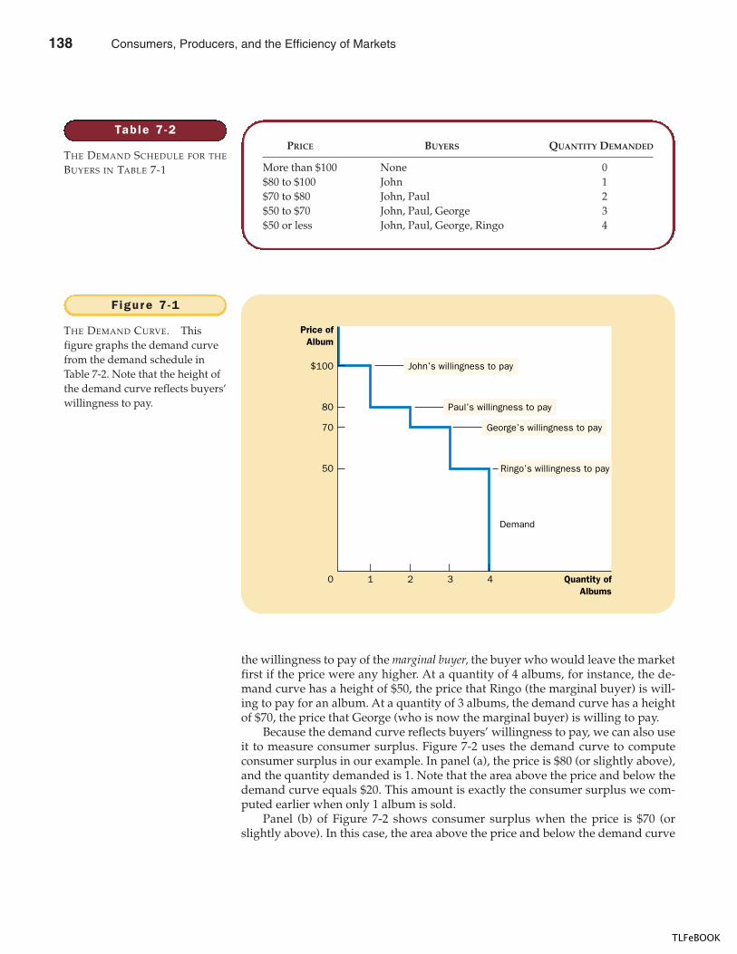
144 PART THREE SUPPLY AND DEMAND I I : MARKETS AND WELFARE
the willingness to pay of the marginal buyer, the buyer who would leave the marketfirst if the price were any higher. At a quantity of 4 albums, for instance, the de-mand curve has a height of $50, the price that Ringo (the marginal buyer) is will-ing to pay for an album. At a quantity of 3 albums, the demand curve has a heightof $70, the price that George (who is now the marginal buyer) is willing to pay.
Because the demand curve reflects buyers’ willingness to pay, we can also useit to measure consumer surplus. Figure 7-2 uses the demand curve to computeconsumer surplus in our example. In panel (a), the price is $80 (or slightly above),and the quantity demanded is 1. Note that the area above the price and below thedemand curve equals $20. This amount is exactly the consumer surplus we com-puted earlier when only 1 album is sold.
Panel (b) of Figure 7-2 shows consumer surplus when the price is $70 (orslightly above). In this case, the area above the price and below the demand curve
Table 7 -2
THE DEMAND SCHEDULE FOR THE
BUYERS IN TABLE 7-1
PRICE BUYERS QUANTITY DEMANDED
More than $100 None 0$80 to $100 John 1$70 to $80 John, Paul 2$50 to $70 John, Paul, George 3$50 or less John, Paul, George, Ringo 4
Price ofAlbum
50
70
80
0
$100
Quantity ofAlbums
Demand
1 2 3 4
John’s willingness to pay
Paul’s willingness to pay
George’s willingness to pay
Ringo’s willingness to pay
Figure 7 -1
THE DEMAND CURVE. Thisfigure graphs the demand curvefrom the demand schedule inTable 7-2. Note that the height ofthe demand curve reflects buyers’willingness to pay.
138 Consumers, Producers, and the Efficiency of Markets
TLFeBOOK
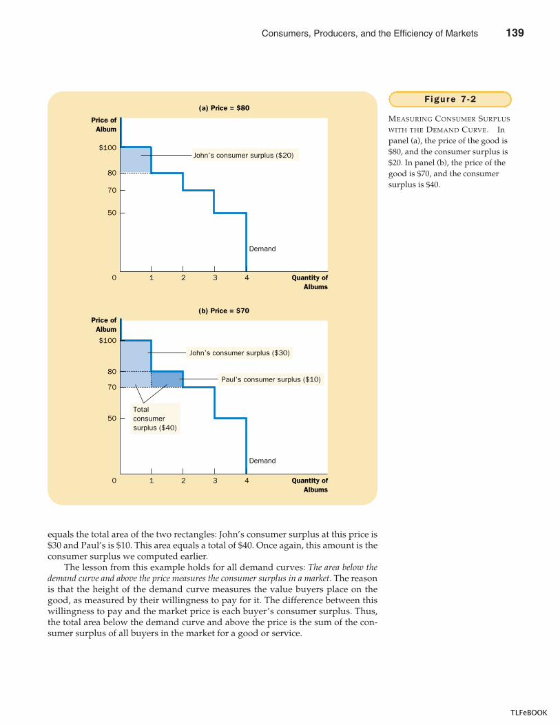
CHAPTER 7 CONSUMERS, PRODUCERS, AND THE EFFICIENCY OF MARKETS 145
equals the total area of the two rectangles: John’s consumer surplus at this price is$30 and Paul’s is $10. This area equals a total of $40. Once again, this amount is theconsumer surplus we computed earlier.
The lesson from this example holds for all demand curves: The area below thedemand curve and above the price measures the consumer surplus in a market. The reasonis that the height of the demand curve measures the value buyers place on thegood, as measured by their willingness to pay for it. The difference between thiswillingness to pay and the market price is each buyer’s consumer surplus. Thus,the total area below the demand curve and above the price is the sum of the con-sumer surplus of all buyers in the market for a good or service.
(b) Price = $70Price of
Album
50
70
80
0
$100
Demand
1 2 3 4
Totalconsumersurplus ($40)
(a) Price = $80
Price ofAlbum
50
70
80
0
$100
Demand
1 2 3 4 Quantity ofAlbums
Quantity ofAlbums
John’s consumer surplus ($30)
Paul’s consumer surplus ($10)
John’s consumer surplus ($20)
Figure 7 -2
MEASURING CONSUMER SURPLUS
WITH THE DEMAND CURVE. Inpanel (a), the price of the good is$80, and the consumer surplus is$20. In panel (b), the price of thegood is $70, and the consumersurplus is $40.
Consumers, Producers, and the Efficiency of Markets 139
TLFeBOOK
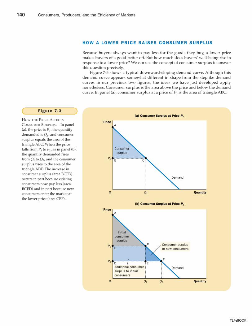
146 PART THREE SUPPLY AND DEMAND I I : MARKETS AND WELFARE
HOW A LOWER PRICE RAISES CONSUMER SURPLUS
Because buyers always want to pay less for the goods they buy, a lower pricemakes buyers of a good better off. But how much does buyers’ well-being rise inresponse to a lower price? We can use the concept of consumer surplus to answerthis question precisely.
Figure 7-3 shows a typical downward-sloping demand curve. Although thisdemand curve appears somewhat different in shape from the steplike demandcurves in our previous two figures, the ideas we have just developed applynonetheless: Consumer surplus is the area above the price and below the demandcurve. In panel (a), consumer surplus at a price of P1 is the area of triangle ABC.
Quantity
(b) Consumer Surplus at Price P2
Quantity
(a) Consumer Surplus at Price P1
Price
0
Demand
P1
A
B C
Consumersurplus
Q1
Price
0
Demand
P1
P2
A
B
Initialconsumersurplus
D
C
EF
Q1 Q2
Consumer surplusto new consumers
Additional consumersurplus to initial consumers
Figure 7 -3
HOW THE PRICE AFFECTS
CONSUMER SURPLUS. In panel(a), the price is P1, the quantitydemanded is Q1, and consumersurplus equals the area of thetriangle ABC. When the pricefalls from P1 to P2, as in panel (b),the quantity demanded risesfrom Q1 to Q2, and the consumersurplus rises to the area of thetriangle ADF. The increase inconsumer surplus (area BCFD)occurs in part because existingconsumers now pay less (areaBCED) and in part because newconsumers enter the market atthe lower price (area CEF).
140 Consumers, Producers, and the Efficiency of Markets
TLFeBOOK
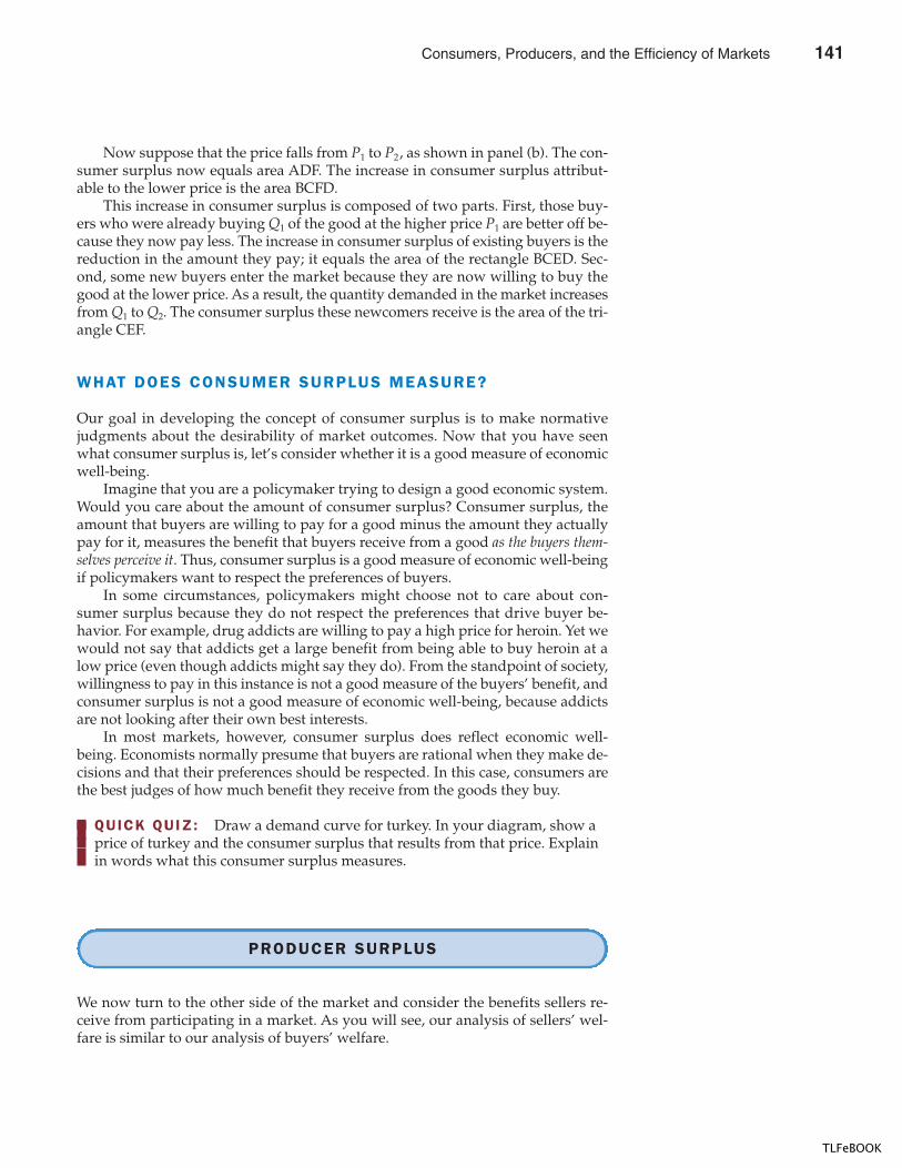
CHAPTER 7 CONSUMERS, PRODUCERS, AND THE EFFICIENCY OF MARKETS 147
Now suppose that the price falls from P1 to P2, as shown in panel (b). The con-sumer surplus now equals area ADF. The increase in consumer surplus attribut-able to the lower price is the area BCFD.
This increase in consumer surplus is composed of two parts. First, those buy-ers who were already buying Q1 of the good at the higher price P1 are better off be-cause they now pay less. The increase in consumer surplus of existing buyers is thereduction in the amount they pay; it equals the area of the rectangle BCED. Sec-ond, some new buyers enter the market because they are now willing to buy thegood at the lower price. As a result, the quantity demanded in the market increasesfrom Q1 to Q2. The consumer surplus these newcomers receive is the area of the tri-angle CEF.
WHAT DOES CONSUMER SURPLUS MEASURE?
Our goal in developing the concept of consumer surplus is to make normativejudgments about the desirability of market outcomes. Now that you have seenwhat consumer surplus is, let’s consider whether it is a good measure of economicwell-being.
Imagine that you are a policymaker trying to design a good economic system.Would you care about the amount of consumer surplus? Consumer surplus, theamount that buyers are willing to pay for a good minus the amount they actuallypay for it, measures the benefit that buyers receive from a good as the buyers them-selves perceive it. Thus, consumer surplus is a good measure of economic well-beingif policymakers want to respect the preferences of buyers.
In some circumstances, policymakers might choose not to care about con-sumer surplus because they do not respect the preferences that drive buyer be-havior. For example, drug addicts are willing to pay a high price for heroin. Yet wewould not say that addicts get a large benefit from being able to buy heroin at alow price (even though addicts might say they do). From the standpoint of society,willingness to pay in this instance is not a good measure of the buyers’ benefit, andconsumer surplus is not a good measure of economic well-being, because addictsare not looking after their own best interests.
In most markets, however, consumer surplus does reflect economic well-being. Economists normally presume that buyers are rational when they make de-cisions and that their preferences should be respected. In this case, consumers arethe best judges of how much benefit they receive from the goods they buy.
QUICK QUIZ: Draw a demand curve for turkey. In your diagram, show a price of turkey and the consumer surplus that results from that price. Explain in words what this consumer surplus measures.
PRODUCER SURPLUS
We now turn to the other side of the market and consider the benefits sellers re-ceive from participating in a market. As you will see, our analysis of sellers’ wel-fare is similar to our analysis of buyers’ welfare.
Consumers, Producers, and the Efficiency of Markets 141
TLFeBOOK
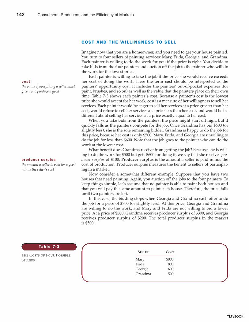
148 PART THREE SUPPLY AND DEMAND I I : MARKETS AND WELFARE
COST AND THE WILL INGNESS TO SELL
Imagine now that you are a homeowner, and you need to get your house painted.You turn to four sellers of painting services: Mary, Frida, Georgia, and Grandma.Each painter is willing to do the work for you if the price is right. You decide totake bids from the four painters and auction off the job to the painter who will dothe work for the lowest price.
Each painter is willing to take the job if the price she would receive exceedsher cost of doing the work. Here the term cost should be interpreted as thepainters’ opportunity cost: It includes the painters’ out-of-pocket expenses (forpaint, brushes, and so on) as well as the value that the painters place on their owntime. Table 7-3 shows each painter’s cost. Because a painter’s cost is the lowestprice she would accept for her work, cost is a measure of her willingness to sell herservices. Each painter would be eager to sell her services at a price greater than hercost, would refuse to sell her services at a price less than her cost, and would be in-different about selling her services at a price exactly equal to her cost.
When you take bids from the painters, the price might start off high, but itquickly falls as the painters compete for the job. Once Grandma has bid $600 (orslightly less), she is the sole remaining bidder. Grandma is happy to do the job forthis price, because her cost is only $500. Mary, Frida, and Georgia are unwilling todo the job for less than $600. Note that the job goes to the painter who can do thework at the lowest cost.
What benefit does Grandma receive from getting the job? Because she is will-ing to do the work for $500 but gets $600 for doing it, we say that she receives pro-ducer surplus of $100. Producer surplus is the amount a seller is paid minus thecost of production. Producer surplus measures the benefit to sellers of participat-ing in a market.
Now consider a somewhat different example. Suppose that you have twohouses that need painting. Again, you auction off the jobs to the four painters. Tokeep things simple, let’s assume that no painter is able to paint both houses andthat you will pay the same amount to paint each house. Therefore, the price fallsuntil two painters are left.
In this case, the bidding stops when Georgia and Grandma each offer to dothe job for a price of $800 (or slightly less). At this price, Georgia and Grandmaare willing to do the work, and Mary and Frida are not willing to bid a lowerprice. At a price of $800, Grandma receives producer surplus of $300, and Georgiareceives producer surplus of $200. The total producer surplus in the marketis $500.
Table 7 -3
THE COSTS OF FOUR POSSIBLE
SELLERS
SELLER COST
Mary $900Frida 800Georgia 600Grandma 500
costthe value of everything a seller mustgive up to produce a good
producer surp lusthe amount a seller is paid for a goodminus the seller’s cost
142 Consumers, Producers, and the Efficiency of Markets
TLFeBOOK
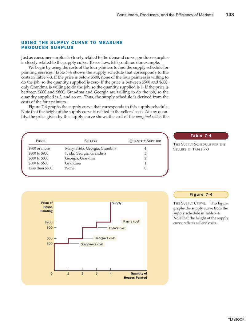
CHAPTER 7 CONSUMERS, PRODUCERS, AND THE EFFICIENCY OF MARKETS 149
USING THE SUPPLY CURVE TO MEASUREPRODUCER SURPLUS
Just as consumer surplus is closely related to the demand curve, producer surplusis closely related to the supply curve. To see how, let’s continue our example.
We begin by using the costs of the four painters to find the supply schedule forpainting services. Table 7-4 shows the supply schedule that corresponds to thecosts in Table 7-3. If the price is below $500, none of the four painters is willing todo the job, so the quantity supplied is zero. If the price is between $500 and $600,only Grandma is willing to do the job, so the quantity supplied is 1. If the price isbetween $600 and $800, Grandma and Georgia are willing to do the job, so thequantity supplied is 2, and so on. Thus, the supply schedule is derived from thecosts of the four painters.
Figure 7-4 graphs the supply curve that corresponds to this supply schedule.Note that the height of the supply curve is related to the sellers’ costs. At any quan-tity, the price given by the supply curve shows the cost of the marginal seller, the
Table 7 -4
THE SUPPLY SCHEDULE FOR THE
SELLERS IN TABLE 7-3
PRICE SELLERS QUANTITY SUPPLIED
$900 or more Mary, Frida, Georgia, Grandma 4$800 to $900 Frida, Georgia, Grandma 3$600 to $800 Georgia, Grandma 2$500 to $600 Grandma 1Less than $500 None 0
Price ofHouse
Painting
500
800
$900
0 Quantity ofHouses Painted
600
1 2 3 4
Supply
Mary’s cost
Frida’s cost
Georgia’s cost
Grandma’s cost
Figure 7 -4
THE SUPPLY CURVE. This figuregraphs the supply curve from thesupply schedule in Table 7-4.Note that the height of the supplycurve reflects sellers’ costs.
Consumers, Producers, and the Efficiency of Markets 143
TLFeBOOK
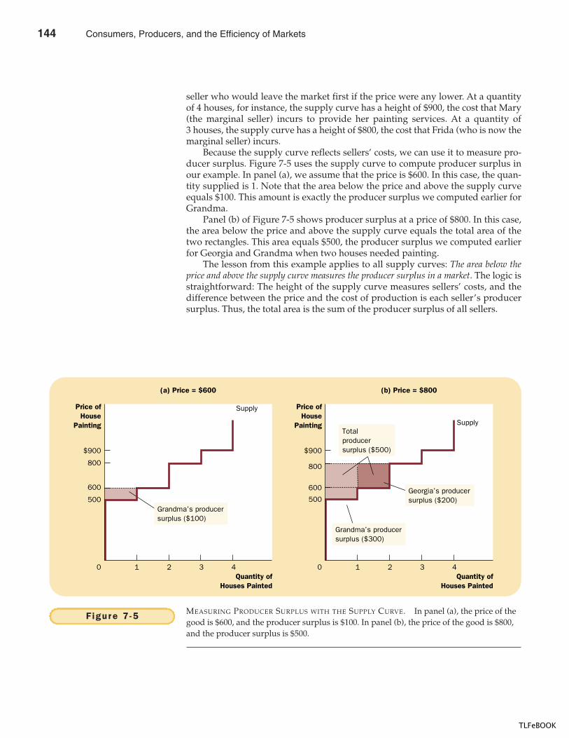
150 PART THREE SUPPLY AND DEMAND I I : MARKETS AND WELFARE
seller who would leave the market first if the price were any lower. At a quantityof 4 houses, for instance, the supply curve has a height of $900, the cost that Mary(the marginal seller) incurs to provide her painting services. At a quantity of3 houses, the supply curve has a height of $800, the cost that Frida (who is now themarginal seller) incurs.
Because the supply curve reflects sellers’ costs, we can use it to measure pro-ducer surplus. Figure 7-5 uses the supply curve to compute producer surplus inour example. In panel (a), we assume that the price is $600. In this case, the quan-tity supplied is 1. Note that the area below the price and above the supply curveequals $100. This amount is exactly the producer surplus we computed earlier forGrandma.
Panel (b) of Figure 7-5 shows producer surplus at a price of $800. In this case,the area below the price and above the supply curve equals the total area of thetwo rectangles. This area equals $500, the producer surplus we computed earlierfor Georgia and Grandma when two houses needed painting.
The lesson from this example applies to all supply curves: The area below theprice and above the supply curve measures the producer surplus in a market. The logic isstraightforward: The height of the supply curve measures sellers’ costs, and thedifference between the price and the cost of production is each seller’s producersurplus. Thus, the total area is the sum of the producer surplus of all sellers.
Quantity ofHouses Painted
Quantity ofHouses Painted
Price ofHouse
Painting
500
800
$900
0
Supply
600
1 2 3 4
(b) Price = $800
Price ofHouse
Painting
500
800
$900
0
600
1 2 3 4
(a) Price = $600
Supply
Grandma’s producersurplus ($100)
Georgia’s producersurplus ($200)
Grandma’s producersurplus ($300)
Totalproducersurplus ($500)
Figure 7 -5 MEASURING PRODUCER SURPLUS WITH THE SUPPLY CURVE. In panel (a), the price of thegood is $600, and the producer surplus is $100. In panel (b), the price of the good is $800,and the producer surplus is $500.
144 Consumers, Producers, and the Efficiency of Markets
TLFeBOOK
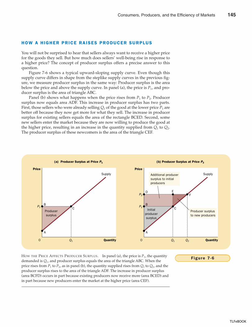
CHAPTER 7 CONSUMERS, PRODUCERS, AND THE EFFICIENCY OF MARKETS 151
HOW A HIGHER PRICE RAISES PRODUCER SURPLUS
You will not be surprised to hear that sellers always want to receive a higher pricefor the goods they sell. But how much does sellers’ well-being rise in response toa higher price? The concept of producer surplus offers a precise answer to thisquestion.
Figure 7-6 shows a typical upward-sloping supply curve. Even though thissupply curve differs in shape from the steplike supply curves in the previous fig-ure, we measure producer surplus in the same way: Producer surplus is the areabelow the price and above the supply curve. In panel (a), the price is P1, and pro-ducer surplus is the area of triangle ABC.
Panel (b) shows what happens when the price rises from P1 to P2. Producersurplus now equals area ADF. This increase in producer surplus has two parts.First, those sellers who were already selling Q1 of the good at the lower price P1 arebetter off because they now get more for what they sell. The increase in producersurplus for existing sellers equals the area of the rectangle BCED. Second, somenew sellers enter the market because they are now willing to produce the good atthe higher price, resulting in an increase in the quantity supplied from Q1 to Q2.The producer surplus of these newcomers is the area of the triangle CEF.
Quantity
(b) Producer Surplus at Price P2
Quantity
(a) Producer Surplus at Price P1
Price
0
Supply
B
A
CProducersurplus
Q1
Price
0
P2
P1B
CP1
Supply
A
D
Initialproducersurplus
EF
Q1 Q2
Producer surplusto new producers
Additional producersurplus to initialproducers
Figure 7 -6HOW THE PRICE AFFECTS PRODUCER SURPLUS. In panel (a), the price is P1, the quantitydemanded is Q1, and producer surplus equals the area of the triangle ABC. When theprice rises from P1 to P2, as in panel (b), the quantity supplied rises from Q1 to Q2, and theproducer surplus rises to the area of the triangle ADF. The increase in producer surplus(area BCFD) occurs in part because existing producers now receive more (area BCED) andin part because new producers enter the market at the higher price (area CEF).
Consumers, Producers, and the Efficiency of Markets 145
TLFeBOOK
152 PART THREE SUPPLY AND DEMAND I I : MARKETS AND WELFARE
As this analysis shows, we use producer surplus to measure the well-being ofsellers in much the same way as we use consumer surplus to measure the well-being of buyers. Because these two measures of economic welfare are so similar, itis natural to use them together. And, indeed, that is exactly what we do in the nextsection.
QUICK QUIZ: Draw a supply curve for turkey. In your diagram, show a price of turkey and the producer surplus that results from that price. Explain in words what this producer surplus measures.
MARKET EFFICIENCY
Consumer surplus and producer surplus are the basic tools that economists use tostudy the welfare of buyers and sellers in a market. These tools can help us addressa fundamental economic question: Is the allocation of resources determined by freemarkets in any way desirable?
THE BENEVOLENT SOCIAL PLANNER
To evaluate market outcomes, we introduce into our analysis a new, hypotheticalcharacter, called the benevolent social planner. The benevolent social planner is anall-knowing, all-powerful, well-intentioned dictator. The planner wants to maxi-mize the economic well-being of everyone in society. What do you suppose thisplanner should do? Should he just leave buyers and sellers at the equilibrium thatthey reach naturally on their own? Or can he increase economic well-being byaltering the market outcome in some way?
To answer this question, the planner must first decide how to measure the eco-nomic well-being of a society. One possible measure is the sum of consumer andproducer surplus, which we call total surplus. Consumer surplus is the benefit thatbuyers receive from participating in a market, and producer surplus is the benefitthat sellers receive. It is therefore natural to use total surplus as a measure of soci-ety’s economic well-being.
To better understand this measure of economic well-being, recall how we mea-sure consumer and producer surplus. We define consumer surplus as
Consumer surplus � Value to buyers � Amount paid by buyers.
Similarly, we define producer surplus as
Producer surplus � Amount received by sellers � Cost to sellers.
When we add consumer and producer surplus together, we obtain
Total surplus � Value to buyers � Amount paid by buyers� Amount received by sellers � Cost to sellers.
146 Consumers, Producers, and the Efficiency of Markets
TLFeBOOK
CHAPTER 7 CONSUMERS, PRODUCERS, AND THE EFFICIENCY OF MARKETS 153
The amount paid by buyers equals the amount received by sellers, so the middletwo terms in this expression cancel each other. As a result, we can write total sur-plus as
Total surplus � Value to buyers � Cost to sellers.
Total surplus in a market is the total value to buyers of the goods, as measured bytheir willingness to pay, minus the total cost to sellers of providing those goods.
If an allocation of resources maximizes total surplus, we say that the allocationexhibits efficiency. If an allocation is not efficient, then some of the gains fromtrade among buyers and sellers are not being realized. For example, an allocationis inefficient if a good is not being produced by the sellers with lowest cost. In thiscase, moving production from a high-cost producer to a low-cost producer willlower the total cost to sellers and raise total surplus. Similarly, an allocation is in-efficient if a good is not being consumed by the buyers who value it most highly.In this case, moving consumption of the good from a buyer with a low valuationto a buyer with a high valuation will raise total surplus.
In addition to efficiency, the social planner might also care about equity—thefairness of the distribution of well-being among the various buyers and sellers. Inessence, the gains from trade in a market are like a pie to be distributed among themarket participants. The question of efficiency is whether the pie is as big as pos-sible. The question of equity is whether the pie is divided fairly. Evaluating theequity of a market outcome is more difficult than evaluating the efficiency.Whereas efficiency is an objective goal that can be judged on strictly positivegrounds, equity involves normative judgments that go beyond economics and en-ter into the realm of political philosophy.
In this chapter we concentrate on efficiency as the social planner’s goal. Keepin mind, however, that real policymakers often care about equity as well. That is,they care about both the size of the economic pie and how the pie gets sliced anddistributed among members of society.
EVALUATING THE MARKET EQUIL IBRIUM
Figure 7-7 shows consumer and producer surplus when a market reaches the equi-librium of supply and demand. Recall that consumer surplus equals the areaabove the price and under the demand curve and producer surplus equals the areabelow the price and above the supply curve. Thus, the total area between the sup-ply and demand curves up to the point of equilibrium represents the total surplusfrom this market.
Is this equilibrium allocation of resources efficient? Does it maximize total sur-plus? To answer these questions, keep in mind that when a market is in equilib-rium, the price determines which buyers and sellers participate in the market.Those buyers who value the good more than the price (represented by the segmentAE on the demand curve) choose to buy the good; those buyers who value it lessthan the price (represented by the segment EB) do not. Similarly, those sellerswhose costs are less than the price (represented by the segment CE on the supplycurve) choose to produce and sell the good; those sellers whose costs are greaterthan the price (represented by the segment ED) do not.
These observations lead to two insights about market outcomes:
ef f ic iencythe property of a resource allocationof maximizing the total surplusreceived by all members of society
equ i tythe fairness of the distribution ofwell-being among the members ofsociety
Consumers, Producers, and the Efficiency of Markets 147
TLFeBOOK
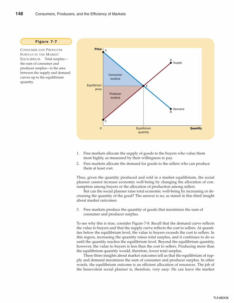
154 PART THREE SUPPLY AND DEMAND I I : MARKETS AND WELFARE
1. Free markets allocate the supply of goods to the buyers who value themmost highly, as measured by their willingness to pay.
2. Free markets allocate the demand for goods to the sellers who can producethem at least cost.
Thus, given the quantity produced and sold in a market equilibrium, the socialplanner cannot increase economic well-being by changing the allocation of con-sumption among buyers or the allocation of production among sellers.
But can the social planner raise total economic well-being by increasing or de-creasing the quantity of the good? The answer is no, as stated in this third insightabout market outcomes:
3. Free markets produce the quantity of goods that maximizes the sum ofconsumer and producer surplus.
To see why this is true, consider Figure 7-8. Recall that the demand curve reflectsthe value to buyers and that the supply curve reflects the cost to sellers. At quanti-ties below the equilibrium level, the value to buyers exceeds the cost to sellers. Inthis region, increasing the quantity raises total surplus, and it continues to do sountil the quantity reaches the equilibrium level. Beyond the equilibrium quantity,however, the value to buyers is less than the cost to sellers. Producing more thanthe equilibrium quantity would, therefore, lower total surplus.
These three insights about market outcomes tell us that the equilibrium of sup-ply and demand maximizes the sum of consumer and producer surplus. In otherwords, the equilibrium outcome is an efficient allocation of resources. The job ofthe benevolent social planner is, therefore, very easy: He can leave the market
Price
Equilibriumprice
0 QuantityEquilibriumquantity
A
Supply
C
BDemand
D
Producersurplus
Consumersurplus
E
Figure 7 -7
CONSUMER AND PRODUCER
SURPLUS IN THE MARKET
EQUILIBRIUM. Total surplus—the sum of consumer andproducer surplus—is the areabetween the supply and demandcurves up to the equilibriumquantity.
148 Consumers, Producers, and the Efficiency of Markets
TLFeBOOK
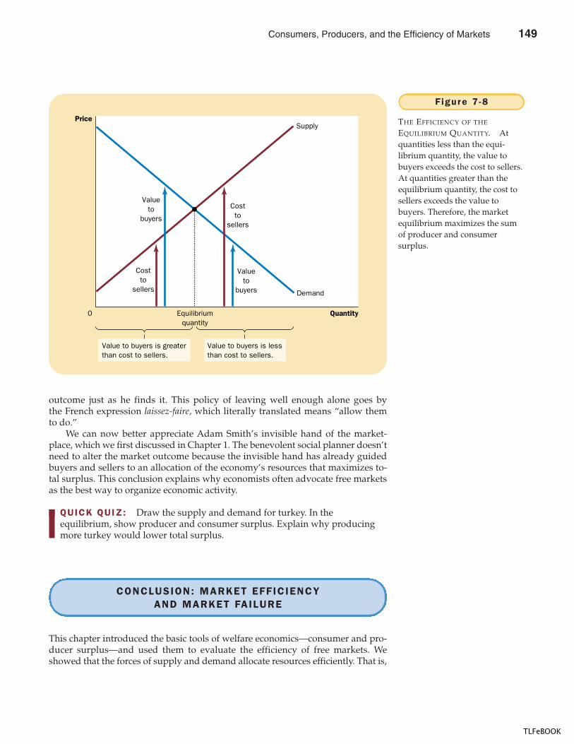
CHAPTER 7 CONSUMERS, PRODUCERS, AND THE EFFICIENCY OF MARKETS 155
outcome just as he finds it. This policy of leaving well enough alone goes bythe French expression laissez-faire, which literally translated means “allow themto do.”
We can now better appreciate Adam Smith’s invisible hand of the market-place, which we first discussed in Chapter 1. The benevolent social planner doesn’tneed to alter the market outcome because the invisible hand has already guidedbuyers and sellers to an allocation of the economy’s resources that maximizes to-tal surplus. This conclusion explains why economists often advocate free marketsas the best way to organize economic activity.
QUICK QUIZ: Draw the supply and demand for turkey. In the equilibrium, show producer and consumer surplus. Explain why producing more turkey would lower total surplus.
CONCLUSION: MARKET EFFICIENCYAND MARKET FAILURE
This chapter introduced the basic tools of welfare economics—consumer and pro-ducer surplus—and used them to evaluate the efficiency of free markets. Weshowed that the forces of supply and demand allocate resources efficiently. That is,
Quantity
Price
0 Equilibriumquantity
Supply
Demand
Costto
sellers
Costto
sellers
Valueto
buyers
Valueto
buyers
Value to buyers is greaterthan cost to sellers.
Value to buyers is lessthan cost to sellers.
Figure 7 -8
THE EFFICIENCY OF THE
EQUILIBRIUM QUANTITY. Atquantities less than the equi-librium quantity, the value tobuyers exceeds the cost to sellers.At quantities greater than theequilibrium quantity, the cost tosellers exceeds the value tobuyers. Therefore, the marketequilibrium maximizes the sumof producer and consumersurplus.
Consumers, Producers, and the Efficiency of Markets 149
TLFeBOOK
156 PART THREE SUPPLY AND DEMAND I I : MARKETS AND WELFARE
even though each buyer and seller in a market is concerned only about his or herown welfare, they are together led by an invisible hand to an equilibrium thatmaximizes the total benefits to buyers and sellers.
A word of warning is in order. To conclude that markets are efficient, we madeseveral assumptions about how markets work. When these assumptions do nothold, our conclusion that the market equilibrium is efficient may no longer be true.As we close this chapter, let’s consider briefly two of the most important of theseassumptions.
First, our analysis assumed that markets are perfectly competitive. In theworld, however, competition is sometimes far from perfect. In some markets, a sin-gle buyer or seller (or a small group of them) may be able to control market prices.This ability to influence prices is called market power. Market power can cause mar-kets to be inefficient because it keeps the price and quantity away from the equi-librium of supply and demand.
Second, our analysis assumed that the outcome in a market matters only to thebuyers and sellers in that market. Yet, in the world, the decisions of buyers and
IF AN ECONOMY IS TO ALLOCATE ITS SCARCE
resources efficiently, goods must get tothose consumers who value them mosthighly. Ticket scalping is one exampleof how markets reach efficient out-comes. Scalpers buy tickets to plays,concerts, and sports events and thensell the tickets at a price above theiroriginal cost. By charging the highestprice the market will bear, scalpers helpensure that consumers with the great-est willingness to pay for the tick-ets actually do get them. In someplaces, however, there is debate overwhether this market activity shouldbe legal.
Ti c k e t s ? S u p p l y M e e t sD e m a n d o n S i d e w a l k
BY JOHN TIERNEY
Ticket scalping has been very good toKevin Thomas, and he makes no apolo-gies. He sees himself as a classic Amer-ican entrepreneur: a high school dropoutfrom the Bronx who taught himself atrade, works seven nights a week, earns$40,000 a year, and at age twenty-sixhas $75,000 in savings, all by providing apublic service outside New York’s the-aters and sports arenas.
He has just one complaint. “I’vebeen busted about 30 times in the lastyear,” he said one recent evening, justafter making $280 at a Knicks game.“You learn to deal with it—I give thecops a fake name, and I pay the fineswhen I have to, but I don’t think it’s fair. Ilook at scalping like working as a stock-broker, buying low and selling high. Ifpeople are willing to pay me the money,what kind of problem is that?”
It is a significant problem to publicofficials in New York and New Jersey,
who are cracking down on streetscalpers like Mr. Thomas and on li-censed ticket brokers. Undercover of-ficers are enforcing new restrictionson reselling tickets at marked-upprices, and the attorneys general of thetwo states are pressing well-publicized
IN THE NEWS
Ticket Scalping
THE INVISIBLE HAND AT WORK
150 Consumers, Producers, and the Efficiency of Markets
TLFeBOOK
CHAPTER 7 CONSUMERS, PRODUCERS, AND THE EFFICIENCY OF MARKETS 157
sellers sometimes affect people who are not participants in the market at all. Pol-lution is the classic example of a market outcome that affects people not in themarket. Such side effects, called externalities, cause welfare in a market to dependon more than just the value to the buyers and the cost to the sellers. Because buy-ers and sellers do not take these side effects into account when deciding how muchto consume and produce, the equilibrium in a market can be inefficient from thestandpoint of society as a whole.
Market power and externalities are examples of a general phenomenon calledmarket failure—the inability of some unregulated markets to allocate resources effi-ciently. When markets fail, public policy can potentially remedy the problem andincrease economic efficiency. Microeconomists devote much effort to studyingwhen market failure is likely and what sorts of policies are best at correcting mar-ket failures. As you continue your study of economics, you will see that the toolsof welfare economics developed here are readily adapted to that endeavor.
Despite the possibility of market failure, the invisible hand of the marketplaceis extraordinarily important. In many markets, the assumptions we made in this
cases against more than a dozen ticketbrokers.
But economists tend to see scalp-ing from Mr. Thomas’s perspective. Tothem, the governments’ crusade makesabout as much sense as the old cam-paigns by Communist authorities against“profiteering.” Economists argue thatthe restrictions inconvenience the public,reduce the audience for cultural andsports events, waste the police’s time,deprive New York City of tens of millionsof dollars of tax revenue, and actuallydrive up the cost of many tickets.
“It is always good politics to poseas defender of the poor by declaring highprices illegal,” says William J. Baumol,the director of the C. V. Starr Center forApplied Economics at New York Univer-sity. “I expect politicians to try to solvethe AIDS crisis by declaring AIDS illegalas well. That would be harmless, be-cause nothing would happen, but whenyou outlaw high prices you create realproblems.”
Dr. Baumol was one of the econo-mists who came up with the idea of sell-
ing same-day Broadway tickets for halfprice at the TKTS booth in Times Square,which theater owners thought danger-ously radical when the booth opened in1973. But the owners have profited byfinding a new clientele for tickets thatwould have gone unsold, an illustrationof the free-market tenet that both buyersand sellers ultimately benefit when priceis adjusted to meet demand.
Economists see another illustrationof that lesson at the Museum of ModernArt, where people wait in line for up totwo hours to buy tickets for the Matisseexhibit. But there is an alternative on thesidewalk: Scalpers who evade the policehave been selling the $12.50 tickets tothe show at prices ranging from $20to $50.
“You don’t have to put a very highvalue on your time to pay $10 or $15 toavoid standing in line for two hours for aMatisse ticket,” said Richard H. Thaler,an economist at Cornell University.“Some people think it’s fairer to makeeveryone stand in line, but that forceseveryone to engage in a totally unpro-
ductive activity, and it discriminates in fa-vor of people who have the most freetime. Scalping gives other people achance, too. I can see no justification foroutlawing it.” . . .
Politicians commonly argue thatwithout anti-scalping laws, tickets wouldbecome unaffordable to most people,but California has no laws against scalp-ing, and ticket prices there are not noto-riously high. And as much as scalperswould like to inflate prices, only a limitednumber of people are willing to pay $100for a ticket. . . .
Legalizing scalping, however, wouldnot necessarily be good news for every-one. Mr. Thomas, for instance, fears thatthe extra competition might put him outof business. But after 16 years—hestarted at age ten outside of YankeeStadium—he is thinking it might be timefor a change anyway.
SOURCE: The New York Times, December 26, 1992,p. A1.
Consumers, Producers, and the Efficiency of Markets 151
TLFeBOOK
158 PART THREE SUPPLY AND DEMAND I I : MARKETS AND WELFARE
chapter work well, and the conclusion of market efficiency applies directly. More-over, our analysis of welfare economics and market efficiency can be used to shedlight on the effects of various government policies. In the next two chapters we ap-ply the tools we have just developed to study two important policy issues—thewelfare effects of taxation and of international trade.
� Consumer surplus equals buyers’ willingness to pay fora good minus the amount they actually pay for it, and itmeasures the benefit buyers get from participating in amarket. Consumer surplus can be computed by findingthe area below the demand curve and above the price.
� Producer surplus equals the amount sellers receive fortheir goods minus their costs of production, and itmeasures the benefit sellers get from participating in amarket. Producer surplus can be computed by findingthe area below the price and above the supply curve.
� An allocation of resources that maximizes the sum ofconsumer and producer surplus is said to be efficient.
Policymakers are often concerned with the efficiency, aswell as the equity, of economic outcomes.
� The equilibrium of supply and demand maximizes thesum of consumer and producer surplus. That is, theinvisible hand of the marketplace leads buyers andsellers to allocate resources efficiently.
� Markets do not allocate resources efficiently in thepresence of market failures such as market power orexternalities.
Summar y
welfare economics, p. 142willingness to pay, p. 142consumer surplus, p. 143
cost, p. 148producer surplus, p. 148
efficiency, p. 153equity, p. 153
Key Concepts
1. Explain how buyers’ willingness to pay, consumersurplus, and the demand curve are related.
2. Explain how sellers’ costs, producer surplus, and thesupply curve are related.
3. In a supply-and-demand diagram, show producer andconsumer surplus in the market equilibrium.
4. What is efficiency? Is it the only goal of economicpolicymakers?
5. What does the invisible hand do?
6. Name two types of market failure. Explain why eachmay cause market outcomes to be inefficient.
Quest ions fo r Rev iew
1. An early freeze in California sours the lemon crop. Whathappens to consumer surplus in the market for lemons?What happens to consumer surplus in the market forlemonade? Illustrate your answers with diagrams.
2. Suppose the demand for French bread rises. Whathappens to producer surplus in the market for Frenchbread? What happens to producer surplus in the marketfor flour? Illustrate your answer with diagrams.
Prob lems and App l icat ions
152 Consumers, Producers, and the Efficiency of Markets
TLFeBOOK
CHAPTER 7 CONSUMERS, PRODUCERS, AND THE EFFICIENCY OF MARKETS 159
3. It is a hot day, and Bert is very thirsty. Here is the valuehe places on a bottle of water:
Value of first bottle $7Value of second bottle 5Value of third bottle 3Value of fourth bottle 1
a. From this information, derive Bert’s demandschedule. Graph his demand curve for bottledwater.
b. If the price of a bottle of water is $4, how manybottles does Bert buy? How much consumersurplus does Bert get from his purchases? ShowBert’s consumer surplus in your graph.
c. If the price falls to $2, how does quantity demandedchange? How does Bert’s consumer surpluschange? Show these changes in your graph.
4. Ernie owns a water pump. Because pumping largeamounts of water is harder than pumping smallamounts, the cost of producing a bottle of water rises ashe pumps more. Here is the cost he incurs to produceeach bottle of water:
Cost of first bottle $1Cost of second bottle 3Cost of third bottle 5Cost of fourth bottle 7
a. From this information, derive Ernie’s supplyschedule. Graph his supply curve for bottled water.
b. If the price of a bottle of water is $4, how manybottles does Ernie produce and sell? How muchproducer surplus does Ernie get from these sales?Show Ernie’s producer surplus in your graph.
c. If the price rises to $6, how does quantity suppliedchange? How does Ernie’s producer surpluschange? Show these changes in your graph.
5. Consider a market in which Bert from Problem 3 is thebuyer and Ernie from Problem 4 is the seller.a. Use Ernie’s supply schedule and Bert’s demand
schedule to find the quantity supplied and quantitydemanded at prices of $2, $4, and $6. Which ofthese prices brings supply and demand intoequilibrium?
b. What are consumer surplus, producer surplus, andtotal surplus in this equilibrium?
c. If Ernie produced and Bert consumed one lessbottle of water, what would happen to totalsurplus?
d. If Ernie produced and Bert consumed oneadditional bottle of water, what would happen tototal surplus?
6. The cost of producing stereo systems has fallen over thepast several decades. Let’s consider some implicationsof this fact.a. Use a supply-and-demand diagram to show the
effect of falling production costs on the price andquantity of stereos sold.
b. In your diagram, show what happens to consumersurplus and producer surplus.
c. Suppose the supply of stereos is very elastic. Whobenefits most from falling production costs—consumers or producers of stereos?
7. There are four consumers willing to pay the followingamounts for haircuts:
Jerry: $7 Oprah: $2 Sally Jessy: $8 Montel: $5
There are four haircutting businesses with the followingcosts:
Firm A: $3 Firm B: $6 Firm C: $4 Firm D: $2
Each firm has the capacity to produce only one haircut.For efficiency, how many haircuts should be given?Which businesses should cut hair, and which consumersshould have their hair cut? How large is the maximumpossible total surplus?
8. Suppose a technological advance reduces the cost ofmaking computers.a. Use a supply-and-demand diagram to show what
happens to price, quantity, consumer surplus, andproducer surplus in the market for computers.
b. Computers and adding machines are substitutes.Use a supply-and-demand diagram to show whathappens to price, quantity, consumer surplus,and producer surplus in the market for addingmachines. Should adding machine producers behappy or sad about the technological advance incomputers?
c. Computers and software are complements. Use asupply-and-demand diagram to show whathappens to price, quantity, consumer surplus, andproducer surplus in the market for software.Should software producers be happy or sad aboutthe technological advance in computers?
d. Does this analysis help explain why Bill Gates, asoftware producer, is one of the world’s richestmen?
Consumers, Producers, and the Efficiency of Markets 153
TLFeBOOK
160 PART THREE SUPPLY AND DEMAND I I : MARKETS AND WELFARE
9. Consider how health insurance affects the quantity ofhealth care services performed. Suppose that the typicalmedical procedure has a cost of $100, yet a person withhealth insurance pays only $20 out-of-pocket when shechooses to have an additional procedure performed.Her insurance company pays the remaining $80. (Theinsurance company will recoup the $80 through higherpremiums for everybody, but the share paid by thisindividual is small.)a. Draw the demand curve in the market for medical
care. (In your diagram, the horizontal axis shouldrepresent the number of medical procedures.) Showthe quantity of procedures demanded if eachprocedure has a price of $100.
b. On your diagram, show the quantity of proceduresdemanded if consumers pay only $20 perprocedure. If the cost of each procedure to society istruly $100, and if individuals have health insuranceas just described, will the number of proceduresperformed maximize total surplus? Explain.
c. Economists often blame the health insurancesystem for excessive use of medical care. Givenyour analysis, why might the use of care be viewedas “excessive”?
d. What sort of policies might prevent this excessiveuse?
10. Many parts of California experienced a severe droughtin the late 1980s and early 1990s.a. Use a diagram of the water market to show the
effects of the drought on the equilibrium price andquantity of water.
b. Many communities did not allow the price of waterto change, however. What is the effect of this policyon the water market? Show on your diagram anysurplus or shortage that arises.
c. A 1991 op-ed piece in The Wall Street Journal statedthat “all Los Angeles residents are required to cuttheir water usage by 10 percent as of March 1 andanother 5 percent starting May 1, based on their1986 consumption levels.” The author criticized thispolicy on both efficiency and equity grounds,saying “not only does such a policy reward familieswho ‘wasted’ more water back in 1986, it does littleto encourage consumers who could make moredrastic reductions, [and] . . . punishes consumerswho cannot so readily reduce their water use.” Inwhat way is the Los Angeles system for allocatingwater inefficient? In what way does the systemseem unfair?
d. Suppose instead that Los Angeles allowed the priceof water to increase until the quantity demandedequaled the quantity supplied. Would the resultingallocation of water be more efficient? In your view,would it be more or less fair than the proportionatereductions in water use mentioned in thenewspaper article? What could be done to make themarket solution more fair?
154 Consumers, Producers, and the Efficiency of Markets
TLFeBOOK
IN THIS CHAPTERYOU WILL . . .
Examine how taxrevenue and
deadweight loss var y wi th the s i ze
o f a tax
Cons ider why sometaxes have la r gerdeadweight losses
than others
Examine how taxesreduce consumer
and producer surp lus
Learn the meaningand causes o f thedeadweight loss o f
a tax
Taxes are often a source of heated political debate. In 1776 the anger of the Ameri-can colonies over British taxes sparked the American Revolution. More than twocenturies later Ronald Reagan was elected president on a platform of large cuts inpersonal income taxes, and during his eight years in the White House the top taxrate on income fell from 70 percent to 28 percent. In 1992 Bill Clinton was electedin part because incumbent George Bush had broken his 1988 campaign promise,“Read my lips: no new taxes.”
We began our study of taxes in Chapter 6. There we saw how a tax on a goodaffects its price and the quantity sold and how the forces of supply and demand di-vide the burden of a tax between buyers and sellers. In this chapter we extend thisanalysis and look at how taxes affect welfare, the economic well-being of partici-pants in a market.
A P P L I C A T I O N : T H E C O S T S
O F T A X A T I O N
161
155
8
TLFeBOOK
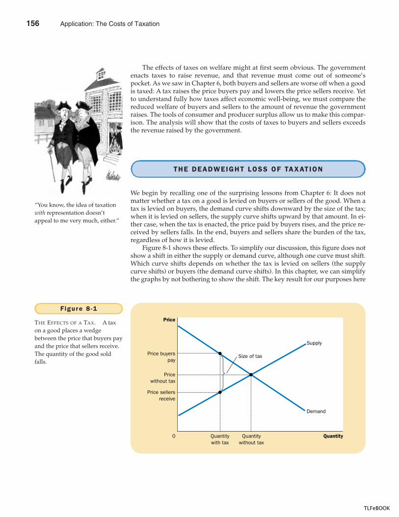
162 PART THREE SUPPLY AND DEMAND I I : MARKETS AND WELFARE
The effects of taxes on welfare might at first seem obvious. The governmentenacts taxes to raise revenue, and that revenue must come out of someone’spocket. As we saw in Chapter 6, both buyers and sellers are worse off when a goodis taxed: A tax raises the price buyers pay and lowers the price sellers receive. Yetto understand fully how taxes affect economic well-being, we must compare thereduced welfare of buyers and sellers to the amount of revenue the governmentraises. The tools of consumer and producer surplus allow us to make this compar-ison. The analysis will show that the costs of taxes to buyers and sellers exceedsthe revenue raised by the government.
THE DEADWEIGHT LOSS OF TAXATION
We begin by recalling one of the surprising lessons from Chapter 6: It does notmatter whether a tax on a good is levied on buyers or sellers of the good. When atax is levied on buyers, the demand curve shifts downward by the size of the tax;when it is levied on sellers, the supply curve shifts upward by that amount. In ei-ther case, when the tax is enacted, the price paid by buyers rises, and the price re-ceived by sellers falls. In the end, buyers and sellers share the burden of the tax,regardless of how it is levied.
Figure 8-1 shows these effects. To simplify our discussion, this figure does notshow a shift in either the supply or demand curve, although one curve must shift.Which curve shifts depends on whether the tax is levied on sellers (the supplycurve shifts) or buyers (the demand curve shifts). In this chapter, we can simplifythe graphs by not bothering to show the shift. The key result for our purposes here
“You know, the idea of taxationwith representation doesn’tappeal to me very much, either.”
Price buyerspay
Size of tax
Pricewithout tax
QuantityQuantitywith tax
0
Price
Price sellersreceive
Quantitywithout tax
Demand
Supply
Figure 8 -1
THE EFFECTS OF A TAX. A taxon a good places a wedgebetween the price that buyers payand the price that sellers receive.The quantity of the good soldfalls.
156 Application: The Costs of Taxation
TLFeBOOK
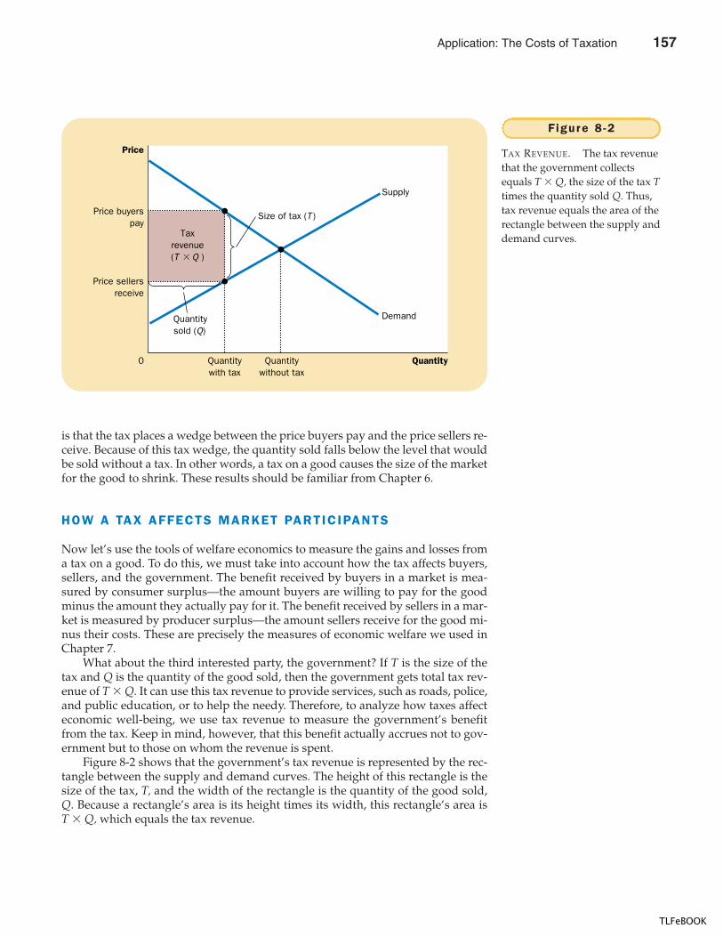
CHAPTER 8 APPLICATION: THE COSTS OF TAXATION 163
is that the tax places a wedge between the price buyers pay and the price sellers re-ceive. Because of this tax wedge, the quantity sold falls below the level that wouldbe sold without a tax. In other words, a tax on a good causes the size of the marketfor the good to shrink. These results should be familiar from Chapter 6.
HOW A TAX AFFECTS MARKET PARTICIPANTS
Now let’s use the tools of welfare economics to measure the gains and losses froma tax on a good. To do this, we must take into account how the tax affects buyers,sellers, and the government. The benefit received by buyers in a market is mea-sured by consumer surplus—the amount buyers are willing to pay for the goodminus the amount they actually pay for it. The benefit received by sellers in a mar-ket is measured by producer surplus—the amount sellers receive for the good mi-nus their costs. These are precisely the measures of economic welfare we used inChapter 7.
What about the third interested party, the government? If T is the size of thetax and Q is the quantity of the good sold, then the government gets total tax rev-enue of T � Q. It can use this tax revenue to provide services, such as roads, police,and public education, or to help the needy. Therefore, to analyze how taxes affecteconomic well-being, we use tax revenue to measure the government’s benefitfrom the tax. Keep in mind, however, that this benefit actually accrues not to gov-ernment but to those on whom the revenue is spent.
Figure 8-2 shows that the government’s tax revenue is represented by the rec-tangle between the supply and demand curves. The height of this rectangle is thesize of the tax, T, and the width of the rectangle is the quantity of the good sold,Q. Because a rectangle’s area is its height times its width, this rectangle’s area isT � Q, which equals the tax revenue.
Price buyerspay
Size of tax (T )
Quantitysold (Q)
Taxrevenue(T � Q )
QuantityQuantitywith tax
0
Price
Price sellersreceive
Quantitywithout tax
Demand
Supply
Figure 8 -2
TAX REVENUE. The tax revenuethat the government collectsequals T � Q, the size of the tax Ttimes the quantity sold Q. Thus,tax revenue equals the area of therectangle between the supply anddemand curves.
Application: The Costs of Taxation 157
TLFeBOOK
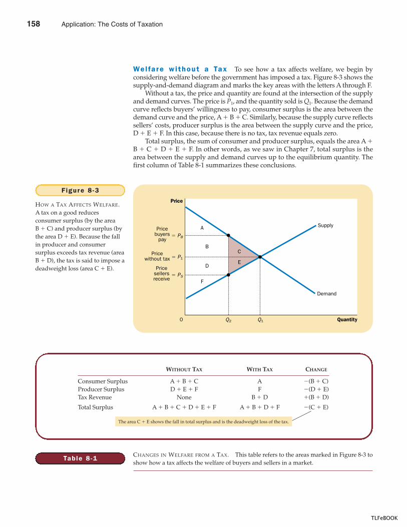
164 PART THREE SUPPLY AND DEMAND I I : MARKETS AND WELFARE
Wel fa r e w i thout a Tax To see how a tax affects welfare, we begin byconsidering welfare before the government has imposed a tax. Figure 8-3 shows thesupply-and-demand diagram and marks the key areas with the letters A through F.
Without a tax, the price and quantity are found at the intersection of the supplyand demand curves. The price is P1, and the quantity sold is Q1. Because the demandcurve reflects buyers’ willingness to pay, consumer surplus is the area between thedemand curve and the price, A � B � C. Similarly, because the supply curve reflectssellers’ costs, producer surplus is the area between the supply curve and the price,D � E � F. In this case, because there is no tax, tax revenue equals zero.
Total surplus, the sum of consumer and producer surplus, equals the area A �B � C � D � E � F. In other words, as we saw in Chapter 7, total surplus is thearea between the supply and demand curves up to the equilibrium quantity. Thefirst column of Table 8-1 summarizes these conclusions.
� PB
A
F
B
D
C
E� P1
QuantityQ20
Price
� PS
Q1
Demand
SupplyPrice
buyerspay
Pricewithout tax
Pricesellersreceive
Figure 8 -3
HOW A TAX AFFECTS WELFARE.A tax on a good reducesconsumer surplus (by the areaB � C) and producer surplus (bythe area D � E). Because the fallin producer and consumersurplus exceeds tax revenue (areaB � D), the tax is said to impose adeadweight loss (area C � E).
Table 8 -1
WITHOUT TAX WITH TAX CHANGE
Consumer Surplus A � B � C A �(B � C)Producer Surplus D � E � F F �(D � E)Tax Revenue None B � D �(B � D)
Total Surplus A � B � C � D � E � F A � B � D � F �(C � E)
CHANGES IN WELFARE FROM A TAX. This table refers to the areas marked in Figure 8-3 toshow how a tax affects the welfare of buyers and sellers in a market.
The area C � E shows the fall in total surplus and is the deadweight loss of the tax.
158 Application: The Costs of Taxation
TLFeBOOK
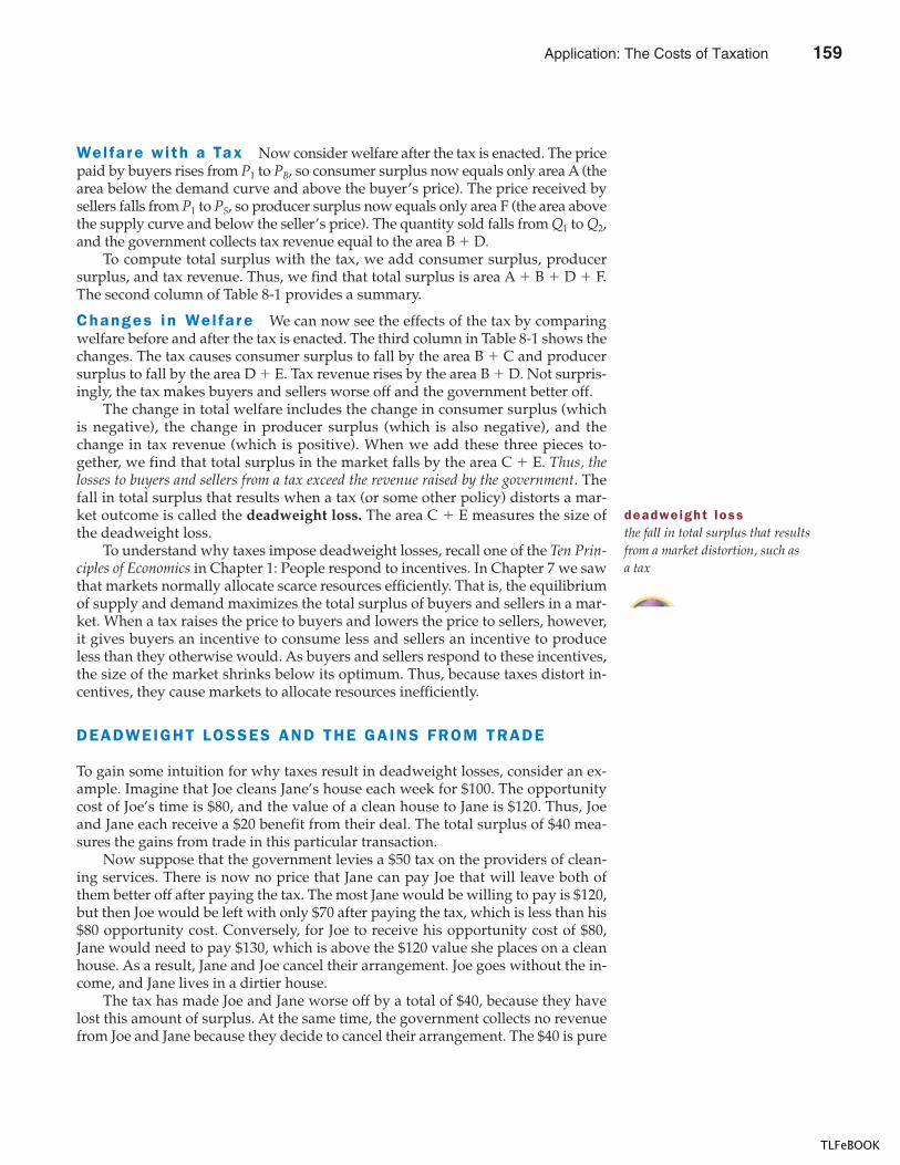
CHAPTER 8 APPLICATION: THE COSTS OF TAXATION 165
Wel fare with a Tax Now consider welfare after the tax is enacted. The pricepaid by buyers rises from P1 to PB, so consumer surplus now equals only area A (thearea below the demand curve and above the buyer’s price). The price received bysellers falls from P1 to PS, so producer surplus now equals only area F (the area abovethe supply curve and below the seller’s price). The quantity sold falls from Q1 to Q2,and the government collects tax revenue equal to the area B � D.
To compute total surplus with the tax, we add consumer surplus, producersurplus, and tax revenue. Thus, we find that total surplus is area A � B � D � F.The second column of Table 8-1 provides a summary.
Changes in Wel fa r e We can now see the effects of the tax by comparingwelfare before and after the tax is enacted. The third column in Table 8-1 shows thechanges. The tax causes consumer surplus to fall by the area B � C and producersurplus to fall by the area D � E. Tax revenue rises by the area B � D. Not surpris-ingly, the tax makes buyers and sellers worse off and the government better off.
The change in total welfare includes the change in consumer surplus (whichis negative), the change in producer surplus (which is also negative), and thechange in tax revenue (which is positive). When we add these three pieces to-gether, we find that total surplus in the market falls by the area C � E. Thus, thelosses to buyers and sellers from a tax exceed the revenue raised by the government. Thefall in total surplus that results when a tax (or some other policy) distorts a mar-ket outcome is called the deadweight loss. The area C � E measures the size ofthe deadweight loss.
To understand why taxes impose deadweight losses, recall one of the Ten Prin-ciples of Economics in Chapter 1: People respond to incentives. In Chapter 7 we sawthat markets normally allocate scarce resources efficiently. That is, the equilibriumof supply and demand maximizes the total surplus of buyers and sellers in a mar-ket. When a tax raises the price to buyers and lowers the price to sellers, however,it gives buyers an incentive to consume less and sellers an incentive to produceless than they otherwise would. As buyers and sellers respond to these incentives,the size of the market shrinks below its optimum. Thus, because taxes distort in-centives, they cause markets to allocate resources inefficiently.
DEADWEIGHT LOSSES AND THE GAINS FROM TRADE
To gain some intuition for why taxes result in deadweight losses, consider an ex-ample. Imagine that Joe cleans Jane’s house each week for $100. The opportunitycost of Joe’s time is $80, and the value of a clean house to Jane is $120. Thus, Joeand Jane each receive a $20 benefit from their deal. The total surplus of $40 mea-sures the gains from trade in this particular transaction.
Now suppose that the government levies a $50 tax on the providers of clean-ing services. There is now no price that Jane can pay Joe that will leave both ofthem better off after paying the tax. The most Jane would be willing to pay is $120,but then Joe would be left with only $70 after paying the tax, which is less than his$80 opportunity cost. Conversely, for Joe to receive his opportunity cost of $80,Jane would need to pay $130, which is above the $120 value she places on a cleanhouse. As a result, Jane and Joe cancel their arrangement. Joe goes without the in-come, and Jane lives in a dirtier house.
The tax has made Joe and Jane worse off by a total of $40, because they havelost this amount of surplus. At the same time, the government collects no revenuefrom Joe and Jane because they decide to cancel their arrangement. The $40 is pure
deadweight lossthe fall in total surplus that resultsfrom a market distortion, such asa tax
Application: The Costs of Taxation 159
TLFeBOOK
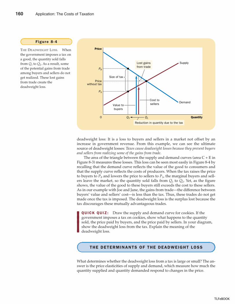
166 PART THREE SUPPLY AND DEMAND I I : MARKETS AND WELFARE
deadweight loss: It is a loss to buyers and sellers in a market not offset by anincrease in government revenue. From this example, we can see the ultimatesource of deadweight losses: Taxes cause deadweight losses because they prevent buyersand sellers from realizing some of the gains from trade.
The area of the triangle between the supply and demand curves (area C + E inFigure 8-3) measures these losses. This loss can be seen most easily in Figure 8-4 byrecalling that the demand curve reflects the value of the good to consumers andthat the supply curve reflects the costs of producers. When the tax raises the priceto buyers to PB and lowers the price to sellers to PS, the marginal buyers and sell-ers leave the market, so the quantity sold falls from Q1 to Q2. Yet, as the figureshows, the value of the good to these buyers still exceeds the cost to these sellers.As in our example with Joe and Jane, the gains from trade—the difference betweenbuyers’ value and sellers’ cost—is less than the tax. Thus, these trades do not getmade once the tax is imposed. The deadweight loss is the surplus lost because thetax discourages these mutually advantageous trades.
QUICK QUIZ: Draw the supply and demand curve for cookies. If the government imposes a tax on cookies, show what happens to the quantity sold, the price paid by buyers, and the price paid by sellers. In your diagram,show the deadweight loss from the tax. Explain the meaning of the deadweight loss.
THE DETERMINANTS OF THE DEADWEIGHT LOSS
What determines whether the deadweight loss from a tax is large or small? The an-swer is the price elasticities of supply and demand, which measure how much thequantity supplied and quantity demanded respond to changes in the price.
PB
Cost tosellersValue to
buyers
Size of taxPrice
without tax
QuantityQ20
Price
PS
Q1
Demand
SupplyLost gainsfrom trade
Reduction in quantity due to the tax
Figure 8 -4
THE DEADWEIGHT LOSS. Whenthe government imposes a tax ona good, the quantity sold fallsfrom Q1 to Q2. As a result, someof the potential gains from tradeamong buyers and sellers do notget realized. These lost gainsfrom trade create thedeadweight loss.
160 Application: The Costs of Taxation
TLFeBOOK
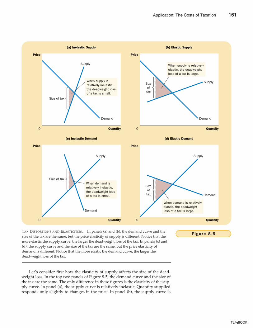
CHAPTER 8 APPLICATION: THE COSTS OF TAXATION 167
Let’s consider first how the elasticity of supply affects the size of the dead-weight loss. In the top two panels of Figure 8-5, the demand curve and the size ofthe tax are the same. The only difference in these figures is the elasticity of the sup-ply curve. In panel (a), the supply curve is relatively inelastic: Quantity suppliedresponds only slightly to changes in the price. In panel (b), the supply curve is
(a) Inelastic Supply (b) Elastic Supply
Price
0 Quantity
Price
0 Quantity
Demand
Supply
(c) Inelastic Demand (d) Elastic Demand
Price
0 Quantity
Price
0 Quantity
Sizeoftax
Size of tax
Demand
Supply
Demand Demand
Supply
SupplySizeoftax
Size of tax
When supply isrelatively inelastic,the deadweight lossof a tax is small.
When supply is relativelyelastic, the deadweightloss of a tax is large.
When demand is relativelyelastic, the deadweightloss of a tax is large.
When demand isrelatively inelastic,the deadweight lossof a tax is small.
Figure 8 -5TAX DISTORTIONS AND ELASTICITIES. In panels (a) and (b), the demand curve and thesize of the tax are the same, but the price elasticity of supply is different. Notice that themore elastic the supply curve, the larger the deadweight loss of the tax. In panels (c) and(d), the supply curve and the size of the tax are the same, but the price elasticity ofdemand is different. Notice that the more elastic the demand curve, the larger thedeadweight loss of the tax.
Application: The Costs of Taxation 161
TLFeBOOK
168 PART THREE SUPPLY AND DEMAND I I : MARKETS AND WELFARE
CASE STUDY THE DEADWEIGHT LOSS DEBATE
Supply, demand, elasticity, deadweight loss—all this economic theory is enoughto make your head spin. But believe it or not, these ideas go to the heart of a pro-found political question: How big should the government be? The reason the de-bate hinges on these concepts is that the larger the deadweight loss of taxation,the larger the cost of any government program. If taxation entails very large dead-weight losses, then these losses are a strong argument for a leaner governmentthat does less and taxes less. By contrast, if taxes impose only small deadweightlosses, then government programs are less costly than they otherwise might be.
So how big are the deadweight losses of taxation? This is a question aboutwhich economists disagree. To see the nature of this disagreement, considerthe most important tax in the U.S. economy—the tax on labor. The Social Se-curity tax, the Medicare tax, and, to a large extent, the federal income tax arelabor taxes. Many state governments also tax labor earnings. A labor tax places awedge between the wage that firms pay and the wage that workers receive. If weadd all forms of labor taxes together, the marginal tax rate on labor income—thetax on the last dollar of earnings—is almost 50 percent for many workers.
Although the size of the labor tax is easy to determine, the deadweight lossof this tax is less straightforward. Economists disagree about whether this 50percent labor tax has a small or a large deadweight loss. This disagreementarises because they hold different views about the elasticity of labor supply.
Economists who argue that labor taxes are not very distorting believe thatlabor supply is fairly inelastic. Most people, they claim, would work full-timeregardless of the wage. If so, the labor supply curve is almost vertical, and a taxon labor has a small deadweight loss.
Economists who argue that labor taxes are highly distorting believe that la-bor supply is more elastic. They admit that some groups of workers may supplytheir labor inelastically but claim that many other groups respond more to in-centives. Here are some examples:
� Many workers can adjust the number of hours they work—for instance, byworking overtime. The higher the wage, the more hours they choose to work.
relatively elastic: Quantity supplied responds substantially to changes in the price.Notice that the deadweight loss, the area of the triangle between the supply anddemand curves, is larger when the supply curve is more elastic.
Similarly, the bottom two panels of Figure 8-5 show how the elasticity of de-mand affects the size of the deadweight loss. Here the supply curve and the size ofthe tax are held constant. In panel (c) the demand curve is relatively inelastic, andthe deadweight loss is small. In panel (d) the demand curve is more elastic, and thedeadweight loss from the tax is larger.
The lesson from this figure is easy to explain. A tax has a deadweight loss be-cause it induces buyers and sellers to change their behavior. The tax raises the pricepaid by buyers, so they consume less. At the same time, the tax lowers the price re-ceived by sellers, so they produce less. Because of these changes in behavior, thesize of the market shrinks below the optimum. The elasticities of supply and de-mand measure how much sellers and buyers respond to the changes in the priceand, therefore, determine how much the tax distorts the market outcome. Hence,the greater the elasticities of supply and demand, the greater the deadweight loss of a tax.
162 Application: The Costs of Taxation
TLFeBOOK
CHAPTER 8 APPLICATION: THE COSTS OF TAXATION 169
� Some families have second earners—often married women with children—with some discretion over whether to do unpaid work at home or paidwork in the marketplace. When deciding whether to take a job, these sec-ond earners compare the benefits of being at home (including savings onthe cost of child care) with the wages they could earn.
� Many of the elderly can choose when to retire, and their decisions are partlybased on the wage. Once they are retired, the wage determines their incen-tive to work part-time.
� Some people consider engaging in illegal economic activity, such as the drugtrade, or working at jobs that pay “under the table” to evade taxes. Econo-mists call this the underground economy. In deciding whether to work in the un-derground economy or at a legitimate job, these potential criminals comparewhat they can earn by breaking the law with the wage they can earn legally.
In each of these cases, the quantity of labor supplied responds to the wage (theprice of labor). Thus, the decisions of these workers are distorted when their la-bor earnings are taxed. Labor taxes encourage workers to work fewer hours,second earners to stay at home, the elderly to retire early, and the unscrupulousto enter the underground economy.
These two views of labor taxation persist to this day. Indeed, whenever yousee two political candidates debating whether the government should providemore services or reduce the tax burden, keep in mind that part of the disagree-ment may rest on different views about the elasticity of labor supply and thedeadweight loss of taxation.
“LET ME TELL YOU WHAT I THINK ABOUT THE ELASTICITY OF LABOR SUPPLY.”
QUICK QUIZ: The demand for beer is more elastic than the demand formilk. Would a tax on beer or a tax on milk have larger deadweight loss? Why?
Application: The Costs of Taxation 163
TLFeBOOK
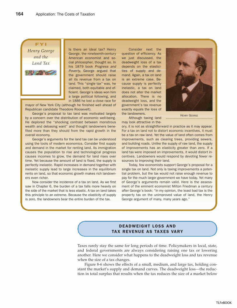
170 PART THREE SUPPLY AND DEMAND I I : MARKETS AND WELFARE
Is there an ideal tax? HenryGeorge, the nineteenth-centuryAmerican economist and so-cial philosopher, thought so. Inhis 1879 book Progress andPoverty, George argued thatthe government should raiseall its revenue from a tax onland. This “single tax” was, heclaimed, both equitable and ef-ficient. George’s ideas won hima large political following, andin 1886 he lost a close race for
mayor of New York City (although he finished well ahead ofRepublican candidate Theodore Roosevelt).
George’s proposal to tax land was motivated largelyby a concern over the distribution of economic well-being.He deplored the “shocking contrast between monstrouswealth and debasing want” and thought landowners bene-fited more than they should from the rapid growth in theoverall economy.
George’s arguments for the land tax can be understoodusing the tools of modern economics. Consider first supplyand demand in the market for renting land. As immigrationcauses the population to rise and technological progresscauses incomes to grow, the demand for land rises overtime. Yet because the amount of land is fixed, the supply isperfectly inelastic. Rapid increases in demand together withinelastic supply lead to large increases in the equilibriumrents on land, so that economic growth makes rich landown-ers even richer.
Now consider the incidence of a tax on land. As we firstsaw in Chapter 6, the burden of a tax falls more heavily onthe side of the market that is less elastic. A tax on land takesthis principle to an extreme. Because the elasticity of supplyis zero, the landowners bear the entire burden of the tax.
Consider next thequestion of efficiency. Aswe just discussed, thedeadweight loss of a taxdepends on the elastici-ties of supply and de-mand. Again, a tax on landis an extreme case. Be-cause supply is perfectlyinelastic, a tax on landdoes not alter the marketallocation. There is nodeadweight loss, and thegovernment’s tax revenueexactly equals the loss ofthe landowners.
Although taxing landmay look attractive in the-ory, it is not as straightforward in practice as it may appear.For a tax on land not to distort economic incentives, it mustbe a tax on raw land. Yet the value of land often comes fromimprovements, such as clearing trees, providing sewers,and building roads. Unlike the supply of raw land, the supplyof improvements has an elasticity greater than zero. If aland tax were imposed on improvements, it would distort in-centives. Landowners would respond by devoting fewer re-sources to improving their land.
Today, few economists support George’s proposal for asingle tax on land. Not only is taxing improvements a poten-tial problem, but the tax would not raise enough revenue topay for the much larger government we have today. Yet manyof George’s arguments remain valid. Here is the assess-ment of the eminent economist Milton Friedman a centuryafter George’s book: “In my opinion, the least bad tax is theproperty tax on the unimproved value of land, the HenryGeorge argument of many, many years ago.”
HENRY GEORGE
FYI
Henry Georgeand the
Land Tax
DEADWEIGHT LOSS AND TAX REVENUE AS TAXES VARY
Taxes rarely stay the same for long periods of time. Policymakers in local, state,and federal governments are always considering raising one tax or loweringanother. Here we consider what happens to the deadweight loss and tax revenuewhen the size of a tax changes.
Figure 8-6 shows the effects of a small, medium, and large tax, holding con-stant the market’s supply and demand curves. The deadweight loss—the reduc-tion in total surplus that results when the tax reduces the size of a market below
164 Application: The Costs of Taxation
TLFeBOOK
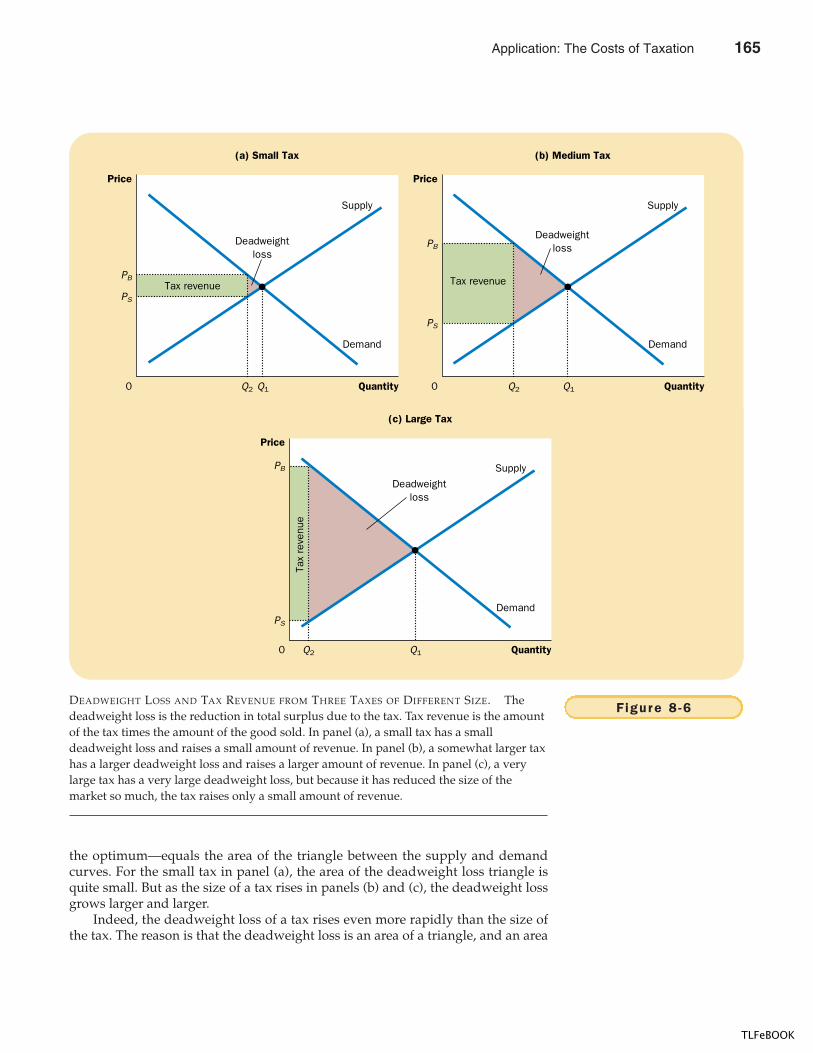
CHAPTER 8 APPLICATION: THE COSTS OF TAXATION 171
the optimum—equals the area of the triangle between the supply and demandcurves. For the small tax in panel (a), the area of the deadweight loss triangle isquite small. But as the size of a tax rises in panels (b) and (c), the deadweight lossgrows larger and larger.
Indeed, the deadweight loss of a tax rises even more rapidly than the size ofthe tax. The reason is that the deadweight loss is an area of a triangle, and an area
Demand
Supply
PB
QuantityQ20
Price
Q1
Demand
Supply
(a) Small Tax
Deadweightloss
Tax revenue Tax revenue
PS
PB
QuantityQ20
Price
Q1
(b) Medium Tax
Deadweightloss
PS
Figure 8 -6DEADWEIGHT LOSS AND TAX REVENUE FROM THREE TAXES OF DIFFERENT SIZE. Thedeadweight loss is the reduction in total surplus due to the tax. Tax revenue is the amountof the tax times the amount of the good sold. In panel (a), a small tax has a smalldeadweight loss and raises a small amount of revenue. In panel (b), a somewhat larger taxhas a larger deadweight loss and raises a larger amount of revenue. In panel (c), a verylarge tax has a very large deadweight loss, but because it has reduced the size of themarket so much, the tax raises only a small amount of revenue.
Tax
reve
nue
PB
QuantityQ20
Price
Q1
Demand
Supply
(c) Large Tax
Deadweightloss
PS
Application: The Costs of Taxation 165
TLFeBOOK
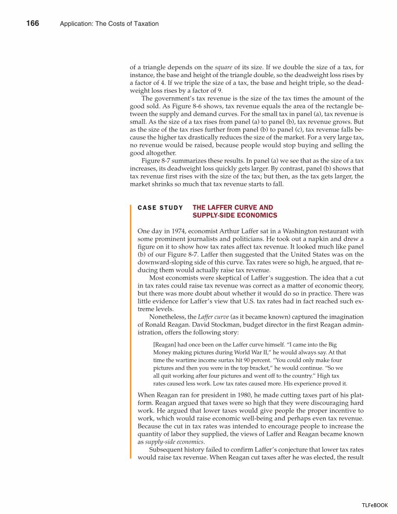
172 PART THREE SUPPLY AND DEMAND I I : MARKETS AND WELFARE
CASE STUDY THE LAFFER CURVE AND SUPPLY-SIDE ECONOMICS
One day in 1974, economist Arthur Laffer sat in a Washington restaurant withsome prominent journalists and politicians. He took out a napkin and drew afigure on it to show how tax rates affect tax revenue. It looked much like panel(b) of our Figure 8-7. Laffer then suggested that the United States was on thedownward-sloping side of this curve. Tax rates were so high, he argued, that re-ducing them would actually raise tax revenue.
Most economists were skeptical of Laffer’s suggestion. The idea that a cutin tax rates could raise tax revenue was correct as a matter of economic theory,but there was more doubt about whether it would do so in practice. There waslittle evidence for Laffer’s view that U.S. tax rates had in fact reached such ex-treme levels.
Nonetheless, the Laffer curve (as it became known) captured the imaginationof Ronald Reagan. David Stockman, budget director in the first Reagan admin-istration, offers the following story:
[Reagan] had once been on the Laffer curve himself. “I came into the BigMoney making pictures during World War II,” he would always say. At thattime the wartime income surtax hit 90 percent. “You could only make fourpictures and then you were in the top bracket,” he would continue. “So weall quit working after four pictures and went off to the country.” High taxrates caused less work. Low tax rates caused more. His experience proved it.
When Reagan ran for president in 1980, he made cutting taxes part of his plat-form. Reagan argued that taxes were so high that they were discouraging hardwork. He argued that lower taxes would give people the proper incentive towork, which would raise economic well-being and perhaps even tax revenue.Because the cut in tax rates was intended to encourage people to increase thequantity of labor they supplied, the views of Laffer and Reagan became knownas supply-side economics.
Subsequent history failed to confirm Laffer’s conjecture that lower tax rateswould raise tax revenue. When Reagan cut taxes after he was elected, the result
of a triangle depends on the square of its size. If we double the size of a tax, forinstance, the base and height of the triangle double, so the deadweight loss rises bya factor of 4. If we triple the size of a tax, the base and height triple, so the dead-weight loss rises by a factor of 9.
The government’s tax revenue is the size of the tax times the amount of thegood sold. As Figure 8-6 shows, tax revenue equals the area of the rectangle be-tween the supply and demand curves. For the small tax in panel (a), tax revenue issmall. As the size of a tax rises from panel (a) to panel (b), tax revenue grows. Butas the size of the tax rises further from panel (b) to panel (c), tax revenue falls be-cause the higher tax drastically reduces the size of the market. For a very large tax,no revenue would be raised, because people would stop buying and selling thegood altogether.
Figure 8-7 summarizes these results. In panel (a) we see that as the size of a taxincreases, its deadweight loss quickly gets larger. By contrast, panel (b) shows thattax revenue first rises with the size of the tax; but then, as the tax gets larger, themarket shrinks so much that tax revenue starts to fall.
166 Application: The Costs of Taxation
TLFeBOOK
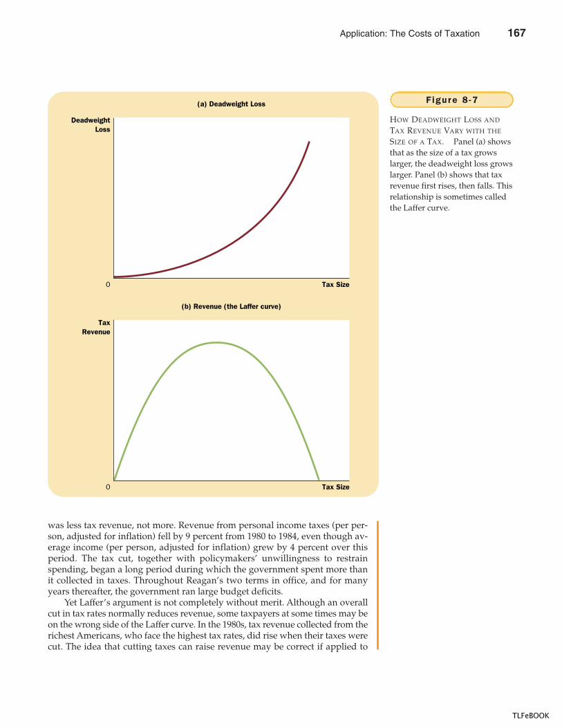
CHAPTER 8 APPLICATION: THE COSTS OF TAXATION 173
was less tax revenue, not more. Revenue from personal income taxes (per per-son, adjusted for inflation) fell by 9 percent from 1980 to 1984, even though av-erage income (per person, adjusted for inflation) grew by 4 percent over thisperiod. The tax cut, together with policymakers’ unwillingness to restrainspending, began a long period during which the government spent more thanit collected in taxes. Throughout Reagan’s two terms in office, and for manyyears thereafter, the government ran large budget deficits.
Yet Laffer’s argument is not completely without merit. Although an overallcut in tax rates normally reduces revenue, some taxpayers at some times may beon the wrong side of the Laffer curve. In the 1980s, tax revenue collected from therichest Americans, who face the highest tax rates, did rise when their taxes werecut. The idea that cutting taxes can raise revenue may be correct if applied to
(a) Deadweight Loss
DeadweightLoss
0 Tax Size
(b) Revenue (the Laffer curve)
TaxRevenue
0 Tax Size
F igure 8 -7
HOW DEADWEIGHT LOSS AND
TAX REVENUE VARY WITH THE
SIZE OF A TAX. Panel (a) showsthat as the size of a tax growslarger, the deadweight loss growslarger. Panel (b) shows that taxrevenue first rises, then falls. Thisrelationship is sometimes calledthe Laffer curve.
Application: The Costs of Taxation 167
TLFeBOOK
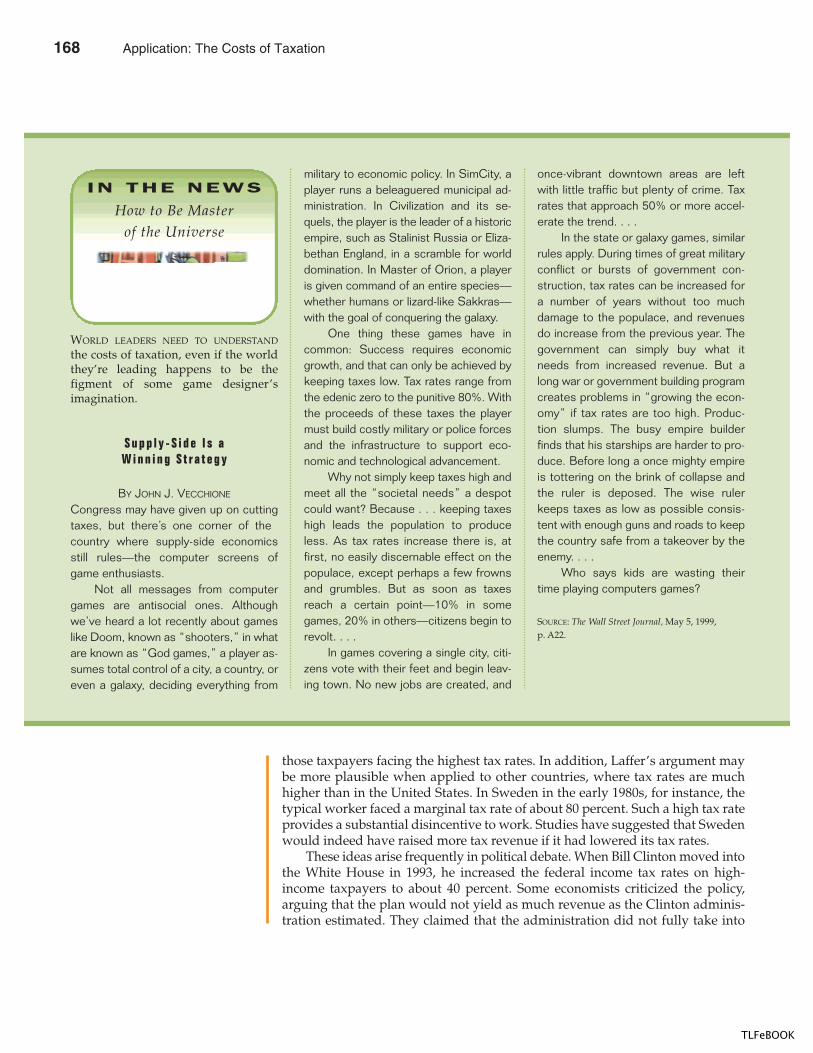
174 PART THREE SUPPLY AND DEMAND I I : MARKETS AND WELFARE
those taxpayers facing the highest tax rates. In addition, Laffer’s argument maybe more plausible when applied to other countries, where tax rates are muchhigher than in the United States. In Sweden in the early 1980s, for instance, thetypical worker faced a marginal tax rate of about 80 percent. Such a high tax rateprovides a substantial disincentive to work. Studies have suggested that Swedenwould indeed have raised more tax revenue if it had lowered its tax rates.
These ideas arise frequently in political debate. When Bill Clinton moved intothe White House in 1993, he increased the federal income tax rates on high-income taxpayers to about 40 percent. Some economists criticized the policy,arguing that the plan would not yield as much revenue as the Clinton adminis-tration estimated. They claimed that the administration did not fully take into
WORLD LEADERS NEED TO UNDERSTAND
the costs of taxation, even if the worldthey’re leading happens to be thefigment of some game designer’simagination.
S u p p l y - S i d e I s aW i n n i n g S t r a t e g y
BY JOHN J. VECCHIONE
Congress may have given up on cuttingtaxes, but there’s one corner of thecountry where supply-side economicsstill rules—the computer screens ofgame enthusiasts.
Not all messages from computergames are antisocial ones. Althoughwe’ve heard a lot recently about gameslike Doom, known as “shooters,” in whatare known as “God games,” a player as-sumes total control of a city, a country, oreven a galaxy, deciding everything from
military to economic policy. In SimCity, aplayer runs a beleaguered municipal ad-ministration. In Civilization and its se-quels, the player is the leader of a historicempire, such as Stalinist Russia or Eliza-bethan England, in a scramble for worlddomination. In Master of Orion, a playeris given command of an entire species—whether humans or lizard-like Sakkras—with the goal of conquering the galaxy.
One thing these games have incommon: Success requires economicgrowth, and that can only be achieved bykeeping taxes low. Tax rates range fromthe edenic zero to the punitive 80%. Withthe proceeds of these taxes the playermust build costly military or police forcesand the infrastructure to support eco-nomic and technological advancement.
Why not simply keep taxes high andmeet all the “societal needs” a despotcould want? Because . . . keeping taxeshigh leads the population to produceless. As tax rates increase there is, atfirst, no easily discernable effect on thepopulace, except perhaps a few frownsand grumbles. But as soon as taxesreach a certain point—10% in somegames, 20% in others—citizens begin torevolt. . . .
In games covering a single city, citi-zens vote with their feet and begin leav-ing town. No new jobs are created, and
once-vibrant downtown areas are leftwith little traffic but plenty of crime. Taxrates that approach 50% or more accel-erate the trend. . . .
In the state or galaxy games, similarrules apply. During times of great militaryconflict or bursts of government con-struction, tax rates can be increased fora number of years without too muchdamage to the populace, and revenuesdo increase from the previous year. Thegovernment can simply buy what itneeds from increased revenue. But along war or government building programcreates problems in “growing the econ-omy” if tax rates are too high. Produc-tion slumps. The busy empire builderfinds that his starships are harder to pro-duce. Before long a once mighty empireis tottering on the brink of collapse andthe ruler is deposed. The wise rulerkeeps taxes as low as possible consis-tent with enough guns and roads to keepthe country safe from a takeover by theenemy. . . .
Who says kids are wasting theirtime playing computers games?
SOURCE: The Wall Street Journal, May 5, 1999,p. A22.
IN THE NEWS
How to Be Masterof the Universe
168 Application: The Costs of Taxation
TLFeBOOK
CHAPTER 8 APPLICATION: THE COSTS OF TAXATION 175
account how taxes alter behavior. Conversely, when Bob Dole challenged BillClinton in the election of 1996, Dole proposed cutting personal income taxes. Al-though Dole rejected the idea that tax cuts would completely pay for themselves,he did claim that 28 percent of the tax cut would be recouped because lower taxrates would lead to more rapid economic growth. Economists debated whetherDole’s 28 percent projection was reasonable, excessively optimistic, or (as Laffermight suggest) excessively pessimistic.
Policymakers disagree about these issues in part because they disagreeabout the size of the relevant elasticities. The more elastic that supply and de-mand are in any market, the more taxes in that market distort behavior, and themore likely it is that a tax cut will raise tax revenue. There is no debate, how-ever, about the general lesson: How much revenue the government gains orloses from a tax change cannot be computed just by looking at tax rates. It alsodepends on how the tax change affects people’s behavior.
QUICK QUIZ: If the government doubles the tax on gasoline, can you be sure that revenue from the gasoline tax will rise? Can you be sure that the deadweight loss from the gasoline tax will rise? Explain.
CONCLUSION
Taxes, Oliver Wendell Holmes once said, are the price we pay for a civilized soci-ety. Indeed, our society cannot exist without some form of taxes. We all expect thegovernment to provide certain services, such as roads, parks, police, and nationaldefense. These public services require tax revenue.
This chapter has shed some light on how high the price of civilized society canbe. One of the Ten Principles of Economics discussed in Chapter 1 is that markets areusually a good way to organize economic activity. When the government imposestaxes on buyers or sellers of a good, however, society loses some of the benefits ofmarket efficiency. Taxes are costly to market participants not only because taxestransfer resources from those participants to the government, but also becausethey alter incentives and distort market outcomes.
� A tax on a good reduces the welfare of buyers andsellers of the good, and the reduction in consumer andproducer surplus usually exceeds the revenue raised bythe government. The fall in total surplus—the sum ofconsumer surplus, producer surplus, and tax revenue—is called the deadweight loss of the tax.
� Taxes have deadweight losses because they causebuyers to consume less and sellers to produce less, andthis change in behavior shrinks the size of the market
below the level that maximizes total surplus. Becausethe elasticities of supply and demand measure howmuch market participants respond to market conditions,larger elasticities imply larger deadweight losses.
� As a tax grows larger, it distorts incentives more, and itsdeadweight loss grows larger. Tax revenue first riseswith the size of a tax. Eventually, however, a larger taxreduces tax revenue because it reduces the size of themarket.
Summar y
Application: The Costs of Taxation 169
TLFeBOOK
176 PART THREE SUPPLY AND DEMAND I I : MARKETS AND WELFARE
1. What happens to consumer and producer surplus whenthe sale of a good is taxed? How does the change inconsumer and producer surplus compare to the taxrevenue? Explain.
2. Draw a supply-and-demand diagram with a tax on thesale of the good. Show the deadweight loss. Show thetax revenue.
3. How do the elasticities of supply and demand affect thedeadweight loss of a tax? Why do they have this effect?
4. Why do experts disagree about whether labor taxeshave small or large deadweight losses?
5. What happens to the deadweight loss and tax revenuewhen a tax is increased?
Quest ions fo r Rev iew
deadweight loss, p. 165
Key Concepts
1. The market for pizza is characterized by a downward-sloping demand curve and an upward-sloping supplycurve.a. Draw the competitive market equilibrium. Label
the price, quantity, consumer surplus, andproducer surplus. Is there any deadweight loss?Explain.
b. Suppose that the government forces each pizzeriato pay a $1 tax on each pizza sold. Illustrate theeffect of this tax on the pizza market, being sure tolabel the consumer surplus, producer surplus,government revenue, and deadweight loss. Howdoes each area compare to the pre-tax case?
c. If the tax were removed, pizza eaters and sellerswould be better off, but the government would losetax revenue. Suppose that consumers andproducers voluntarily transferred some of theirgains to the government. Could all parties(including the government) be better off than theywere with a tax? Explain using the labeled areas inyour graph.
2. Evaluate the following two statements. Do you agree?Why or why not?a. “If the government taxes land, wealthy land-
owners will pass the tax on to their poorer renters.”b. “If the government taxes apartment buildings,
wealthy landlords will pass the tax on to theirpoorer renters.”
3. Evaluate the following two statements. Do you agree?Why or why not?
a. “A tax that has no deadweight loss cannot raise anyrevenue for the government.”
b. “A tax that raises no revenue for the governmentcannot have any deadweight loss.”
4. Consider the market for rubber bands.a. If this market has very elastic supply and very
inelastic demand, how would the burden of a taxon rubber bands be shared between consumers andproducers? Use the tools of consumer surplus andproducer surplus in your answer.
b. If this market has very inelastic supply and veryelastic demand, how would the burden of a tax onrubber bands be shared between consumers andproducers? Contrast your answer with your answerto part (a).
5. Suppose that the government imposes a tax onheating oil.a. Would the deadweight loss from this tax likely be
greater in the first year after it is imposed or in thefifth year? Explain.
b. Would the revenue collected from this tax likely begreater in the first year after it is imposed or in thefifth year? Explain.
6. After economics class one day, your friend suggeststhat taxing food would be a good way to raiserevenue because the demand for food is quite inelastic.In what sense is taxing food a “good” way to raiserevenue? In what sense is it not a “good” way to raiserevenue?
Prob lems and App l icat ions
170 Application: The Costs of Taxation
TLFeBOOK
CHAPTER 8 APPLICATION: THE COSTS OF TAXATION 177
7. Senator Daniel Patrick Moynihan once introduced a billthat would levy a 10,000 percent tax on certain hollow-tipped bullets.a. Do you expect that this tax would raise much
revenue? Why or why not?b. Even if the tax would raise no revenue, what
might be Senator Moynihan’s reason forproposing it?
8. The government places a tax on the purchase of socks.a. Illustrate the effect of this tax on equilibrium price
and quantity in the sock market. Identify thefollowing areas both before and after the impositionof the tax: total spending by consumers, totalrevenue for producers, and government taxrevenue.
b. Does the price received by producers rise or fall?Can you tell whether total receipts for producersrise or fall? Explain.
c. Does the price paid by consumers rise or fall? Canyou tell whether total spending by consumers risesor falls? Explain carefully. (Hint: Think aboutelasticity.) If total consumer spending falls, doesconsumer surplus rise? Explain.
9. Suppose the government currently raises $100 millionthrough a $0.01 tax on widgets, and another $100million through a $0.10 tax on gadgets. If thegovernment doubled the tax rate on widgets andeliminated the tax on gadgets, would it raise moremoney than today, less money, or the same amount ofmoney? Explain.
10. Most states tax the purchase of new cars. Suppose thatNew Jersey currently requires car dealers to pay thestate $100 for each car sold, and plans to increase the taxto $150 per car next year.a. Illustrate the effect of this tax increase on the
quantity of cars sold in New Jersey, the price paidby consumers, and the price received by producers.
b. Create a table that shows the levels of consumersurplus, producer surplus, government revenue,and total surplus both before and after the taxincrease.
c. What is the change in government revenue? Is itpositive or negative?
d. What is the change in deadweight loss? Is itpositive or negative?
e. Give one reason why the demand for cars in NewJersey might be fairly elastic. Does this make theadditional tax more or less likely to increase
government revenue? How might states try toreduce the elasticity of demand?
11. Several years ago the British government imposed a“poll tax” that required each person to pay a flatamount to the government independent of his or herincome or wealth. What is the effect of such a tax oneconomic efficiency? What is the effect on economicequity? Do you think this was a popular tax?
12. This chapter analyzed the welfare effects of a tax on agood. Consider now the opposite policy. Suppose thatthe government subsidizes a good: For each unit of thegood sold, the government pays $2 to the buyer. Howdoes the subsidy affect consumer surplus, producersurplus, tax revenue, and total surplus? Does a subsidylead to a deadweight loss? Explain.
13. (This problem uses some high school algebra and ischallenging.) Suppose that a market is described by thefollowing supply and demand equations:
QS = 2PQD = 300 � P
a. Solve for the equilibrium price and the equilibriumquantity.
b. Suppose that a tax of T is placed on buyers, so thenew demand equation is
QD = 300 � (P � T).
Solve for the new equilibrium. What happens to theprice received by sellers, the price paid by buyers,and the quantity sold?
c. Tax revenue is T � Q. Use your answer to part (b)to solve for tax revenue as a function of T. Graphthis relationship for T between 0 and 300.
d. The deadweight loss of a tax is the area of thetriangle between the supply and demand curves.Recalling that the area of a triangle is 1/2 � base �height, solve for deadweight loss as a function of T.Graph this relationship for T between 0 and 300.(Hint: Looking sideways, the base of thedeadweight loss triangle is T, and the height is thedifference between the quantity sold with the taxand the quantity sold without the tax.)
e. The government now levies a tax on this good of$200 per unit. Is this a good policy? Why or whynot? Can you propose a better policy?
Application: The Costs of Taxation 171
TLFeBOOK

TLFeBOOK
IN THIS CHAPTERYOU WILL . . .
Examine thearguments peop leuse to advocate
t rade r est r ict ions
Learn that the ga insto winners f r om
internat iona l t radeexceed the losses
to losers
Cons ider whatdetermines whethera count r y impor tsor expor ts a good
Examine who winsand who loses f r ominternat iona l t rade
Analyze the wel fa reef fects o f ta r i f fs
and impor t quotas
If you check the labels on the clothes you are now wearing, you will probably findthat some of your clothes were made in another country. A century ago the textilesand clothing industry was a major part of the U.S. economy, but that is no longerthe case. Faced with foreign competitors that could produce quality goods at lowcost, many U.S. firms found it increasingly difficult to produce and sell textiles andclothing at a profit. As a result, they laid off their workers and shut down their fac-tories. Today, much of the textiles and clothing that Americans consume are im-ported from abroad.
The story of the textiles industry raises important questions for economic pol-icy: How does international trade affect economic well-being? Who gains and wholoses from free trade among countries, and how do the gains compare to thelosses?
A P P L I C A T I O N :
I N T E R N A T I O N A L T R A D E
179
173
9
TLFeBOOK
180 PART THREE SUPPLY AND DEMAND I I : MARKETS AND WELFARE
Chapter 3 introduced the study of international trade by applying the princi-ple of comparative advantage. According to this principle, all countries can bene-fit from trading with one another because trade allows each country to specializein doing what it does best. But the analysis in Chapter 3 was incomplete. It did notexplain how the international marketplace achieves these gains from trade or howthe gains are distributed among various economic actors.
We now return to the study of international trade and take up these questions.Over the past several chapters, we have developed many tools for analyzing howmarkets work: supply, demand, equilibrium, consumer surplus, producer surplus,and so on. With these tools we can learn more about the effects of internationaltrade on economic well-being.
THE DETERMINANTS OF TRADE
Consider the market for steel. The steel market is well suited to examining thegains and losses from international trade: Steel is made in many countries aroundthe world, and there is much world trade in steel. Moreover, the steel market is onein which policymakers often consider (and sometimes implement) trade restric-tions in order to protect domestic steel producers from foreign competitors. We ex-amine here the steel market in the imaginary country of Isoland.
THE EQUIL IBRIUM WITHOUT TRADE
As our story begins, the Isolandian steel market is isolated from the rest of theworld. By government decree, no one in Isoland is allowed to import or exportsteel, and the penalty for violating the decree is so large that no one dares try.
Because there is no international trade, the market for steel in Isoland consistssolely of Isolandian buyers and sellers. As Figure 9-1 shows, the domestic price ad-justs to balance the quantity supplied by domestic sellers and the quantity de-manded by domestic buyers. The figure shows the consumer and producersurplus in the equilibrium without trade. The sum of consumer and producersurplus measures the total benefits that buyers and sellers receive from the steelmarket.
Now suppose that, in an election upset, Isoland elects a new president. Thepresident campaigned on a platform of “change” and promised the voters boldnew ideas. Her first act is to assemble a team of economists to evaluate Isolandiantrade policy. She asks them to report back on three questions:
� If the government allowed Isolandians to import and export steel, whatwould happen to the price of steel and the quantity of steel sold in thedomestic steel market?
� Who would gain from free trade in steel and who would lose, and would thegains exceed the losses?
� Should a tariff (a tax on steel imports) or an import quota (a limit on steelimports) be part of the new trade policy?
174 Application: International Trade
TLFeBOOK
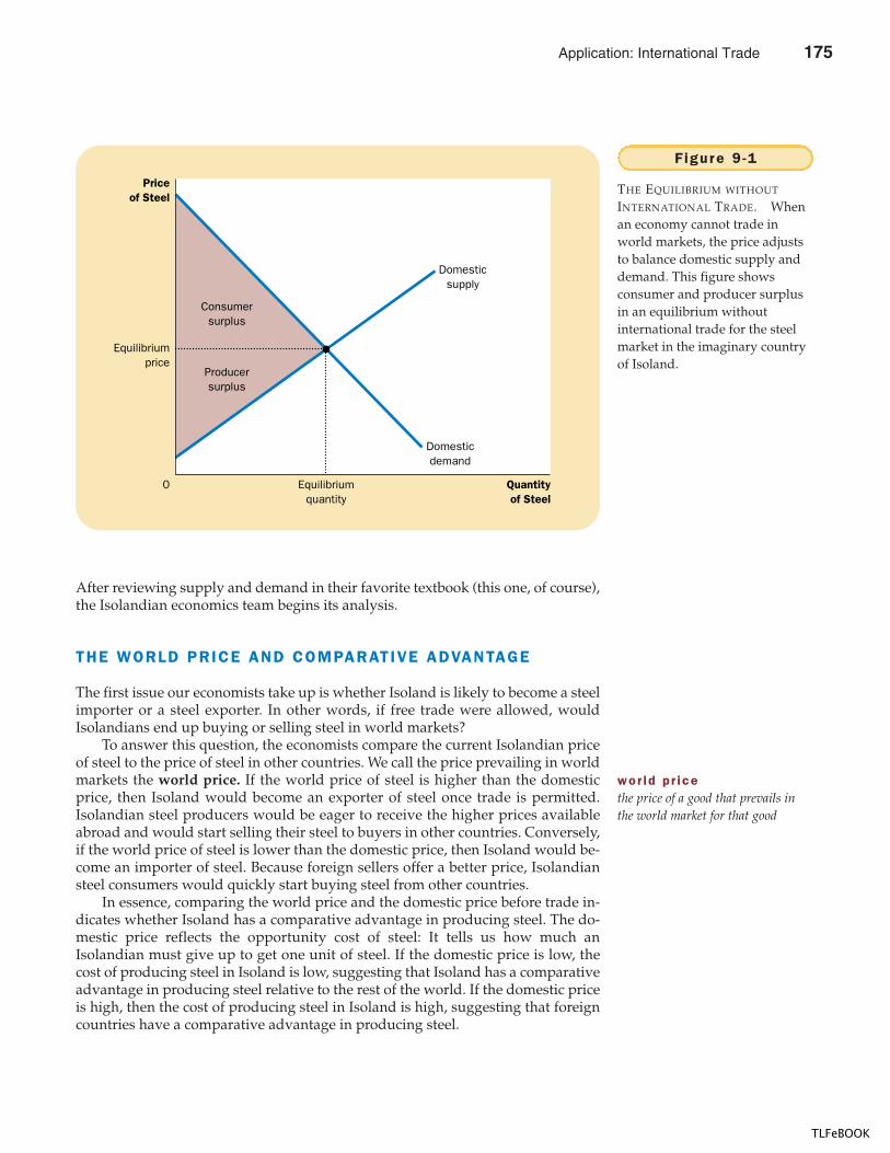
CHAPTER 9 APPLICATION: INTERNATIONAL TRADE 181
After reviewing supply and demand in their favorite textbook (this one, of course),the Isolandian economics team begins its analysis.
THE WORLD PRICE AND COMPARATIVE ADVANTAGE
The first issue our economists take up is whether Isoland is likely to become a steelimporter or a steel exporter. In other words, if free trade were allowed, wouldIsolandians end up buying or selling steel in world markets?
To answer this question, the economists compare the current Isolandian priceof steel to the price of steel in other countries. We call the price prevailing in worldmarkets the world price. If the world price of steel is higher than the domesticprice, then Isoland would become an exporter of steel once trade is permitted.Isolandian steel producers would be eager to receive the higher prices availableabroad and would start selling their steel to buyers in other countries. Conversely,if the world price of steel is lower than the domestic price, then Isoland would be-come an importer of steel. Because foreign sellers offer a better price, Isolandiansteel consumers would quickly start buying steel from other countries.
In essence, comparing the world price and the domestic price before trade in-dicates whether Isoland has a comparative advantage in producing steel. The do-mestic price reflects the opportunity cost of steel: It tells us how much anIsolandian must give up to get one unit of steel. If the domestic price is low, thecost of producing steel in Isoland is low, suggesting that Isoland has a comparativeadvantage in producing steel relative to the rest of the world. If the domestic priceis high, then the cost of producing steel in Isoland is high, suggesting that foreigncountries have a comparative advantage in producing steel.
Priceof Steel
Equilibriumprice
0 Quantityof Steel
Equilibriumquantity
Domesticsupply
Domesticdemand
Producersurplus
Consumersurplus
Figure 9 -1
THE EQUILIBRIUM WITHOUT
INTERNATIONAL TRADE. Whenan economy cannot trade inworld markets, the price adjuststo balance domestic supply anddemand. This figure showsconsumer and producer surplusin an equilibrium withoutinternational trade for the steelmarket in the imaginary countryof Isoland.
wor ld p r icethe price of a good that prevails inthe world market for that good
Application: International Trade 175
TLFeBOOK
182 PART THREE SUPPLY AND DEMAND I I : MARKETS AND WELFARE
As we saw in Chapter 3, trade among nations is ultimately based on compar-ative advantage. That is, trade is beneficial because it allows each nation to spe-cialize in doing what it does best. By comparing the world price and the domesticprice before trade, we can determine whether Isoland is better or worse at pro-ducing steel than the rest of the world.
QUICK QUIZ: The country Autarka does not allow international trade. In Autarka, you can buy a wool suit for 3 ounces of gold. Meanwhile, in neighboring countries, you can buy the same suit for 2 ounces of gold. If Autarka were to allow free trade, would it import or export suits?
THE WINNERS AND LOSERS FROM TRADE
To analyze the welfare effects of free trade, the Isolandian economists begin withthe assumption that Isoland is a small economy compared to the rest of the worldso that its actions have negligible effect on world markets. The small-economy as-sumption has a specific implication for analyzing the steel market: If Isoland is asmall economy, then the change in Isoland’s trade policy will not affect the worldprice of steel. The Isolandians are said to be price takers in the world economy. Thatis, they take the world price of steel as given. They can sell steel at this price andbe exporters or buy steel at this price and be importers.
The small-economy assumption is not necessary to analyze the gains andlosses from international trade. But the Isolandian economists know from experi-ence that this assumption greatly simplifies the analysis. They also know that thebasic lessons do not change in the more complicated case of a large economy.
THE GAINS AND LOSSES OF AN EXPORTING COUNTRY
Figure 9-2 shows the Isolandian steel market when the domestic equilibrium pricebefore trade is below the world price. Once free trade is allowed, the domesticprice rises to equal the world price. No seller of steel would accept less than theworld price, and no buyer would pay more than the world price.
With the domestic price now equal to the world price, the domestic quantitysupplied differs from the domestic quantity demanded. The supply curve showsthe quantity of steel supplied by Isolandian sellers. The demand curve shows thequantity of steel demanded by Isolandian buyers. Because the domestic quantitysupplied is greater than the domestic quantity demanded, Isoland sells steel toother countries. Thus, Isoland becomes a steel exporter.
Although domestic quantity supplied and domestic quantity demanded differ,the steel market is still in equilibrium because there is now another participant inthe market: the rest of the world. One can view the horizontal line at the worldprice as representing the demand for steel from the rest of the world. This demandcurve is perfectly elastic because Isoland, as a small economy, can sell as muchsteel as it wants at the world price.
176 Application: International Trade
TLFeBOOK
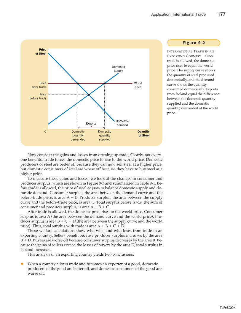
CHAPTER 9 APPLICATION: INTERNATIONAL TRADE 183
Now consider the gains and losses from opening up trade. Clearly, not every-one benefits. Trade forces the domestic price to rise to the world price. Domesticproducers of steel are better off because they can now sell steel at a higher price,but domestic consumers of steel are worse off because they have to buy steel at ahigher price.
To measure these gains and losses, we look at the changes in consumer andproducer surplus, which are shown in Figure 9-3 and summarized in Table 9-1. Be-fore trade is allowed, the price of steel adjusts to balance domestic supply and do-mestic demand. Consumer surplus, the area between the demand curve and thebefore-trade price, is area A � B. Producer surplus, the area between the supplycurve and the before-trade price, is area C. Total surplus before trade, the sum ofconsumer and producer surplus, is area A � B � C.
After trade is allowed, the domestic price rises to the world price. Consumersurplus is area A (the area between the demand curve and the world price). Pro-ducer surplus is area B � C � D (the area between the supply curve and the worldprice). Thus, total surplus with trade is area A � B � C � D.
These welfare calculations show who wins and who loses from trade in anexporting country. Sellers benefit because producer surplus increases by the areaB � D. Buyers are worse off because consumer surplus decreases by the area B. Be-cause the gains of sellers exceed the losses of buyers by the area D, total surplus inIsoland increases.
This analysis of an exporting country yields two conclusions:
� When a country allows trade and becomes an exporter of a good, domesticproducers of the good are better off, and domestic consumers of the good areworse off.
Priceof Steel
Pricebefore trade
Priceafter trade
0 Quantityof Steel
Domesticquantity
demanded
Domesticquantitysupplied
Domesticsupply
Worldprice
DomesticdemandExports
Figure 9 -2
INTERNATIONAL TRADE IN AN
EXPORTING COUNTRY. Oncetrade is allowed, the domesticprice rises to equal the worldprice. The supply curve showsthe quantity of steel produceddomestically, and the demandcurve shows the quantityconsumed domestically. Exportsfrom Isoland equal the differencebetween the domestic quantitysupplied and the domesticquantity demanded at the worldprice.
Application: International Trade 177
TLFeBOOK
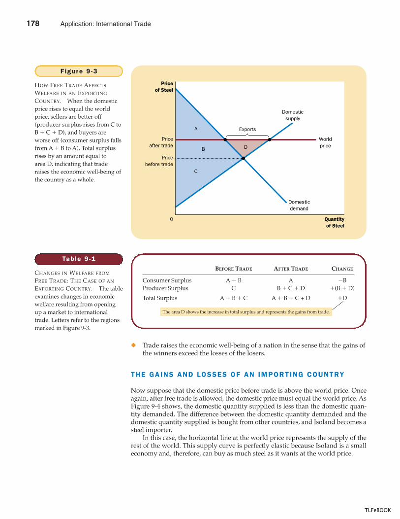
184 PART THREE SUPPLY AND DEMAND I I : MARKETS AND WELFARE
� Trade raises the economic well-being of a nation in the sense that the gains ofthe winners exceed the losses of the losers.
THE GAINS AND LOSSES OF AN IMPORTING COUNTRY
Now suppose that the domestic price before trade is above the world price. Onceagain, after free trade is allowed, the domestic price must equal the world price. AsFigure 9-4 shows, the domestic quantity supplied is less than the domestic quan-tity demanded. The difference between the domestic quantity demanded and thedomestic quantity supplied is bought from other countries, and Isoland becomes asteel importer.
In this case, the horizontal line at the world price represents the supply of therest of the world. This supply curve is perfectly elastic because Isoland is a smalleconomy and, therefore, can buy as much steel as it wants at the world price.
C
B D
A
Priceof Steel
Pricebefore trade
Priceafter trade
0 Quantityof Steel
Domesticsupply
Worldprice
Domesticdemand
Exports
Figure 9 -3
HOW FREE TRADE AFFECTS
WELFARE IN AN EXPORTING
COUNTRY. When the domesticprice rises to equal the worldprice, sellers are better off(producer surplus rises from C toB � C � D), and buyers areworse off (consumer surplus fallsfrom A � B to A). Total surplusrises by an amount equal toarea D, indicating that traderaises the economic well-being ofthe country as a whole.
Table 9 -1
CHANGES IN WELFARE FROM
FREE TRADE: THE CASE OF AN
EXPORTING COUNTRY. The tableexamines changes in economicwelfare resulting from openingup a market to internationaltrade. Letters refer to the regionsmarked in Figure 9-3.
BEFORE TRADE AFTER TRADE CHANGE
Consumer Surplus A � B A �BProducer Surplus C B � C � D �(B � D)
Total Surplus A � B � C A � B � C + D �D
The area D shows the increase in total surplus and represents the gains from trade.
178 Application: International Trade
TLFeBOOK
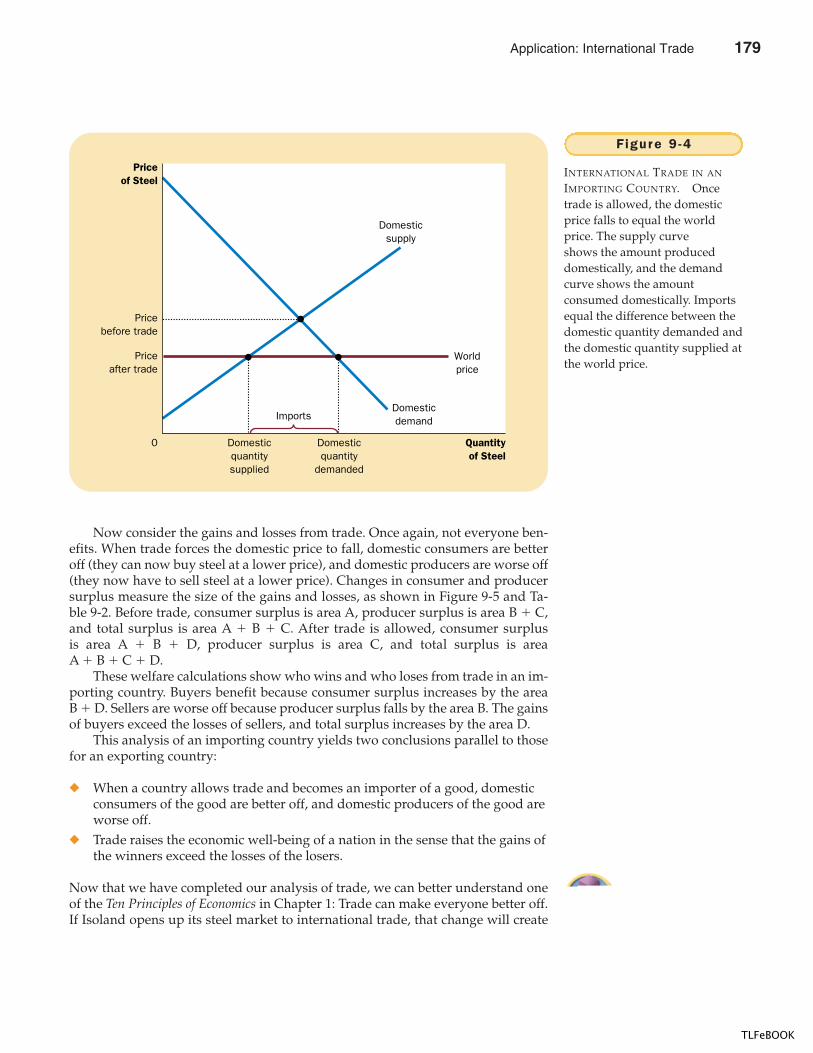
CHAPTER 9 APPLICATION: INTERNATIONAL TRADE 185
Now consider the gains and losses from trade. Once again, not everyone ben-efits. When trade forces the domestic price to fall, domestic consumers are betteroff (they can now buy steel at a lower price), and domestic producers are worse off(they now have to sell steel at a lower price). Changes in consumer and producersurplus measure the size of the gains and losses, as shown in Figure 9-5 and Ta-ble 9-2. Before trade, consumer surplus is area A, producer surplus is area B � C,and total surplus is area A � B � C. After trade is allowed, consumer surplusis area A � B � D, producer surplus is area C, and total surplus is areaA � B � C � D.
These welfare calculations show who wins and who loses from trade in an im-porting country. Buyers benefit because consumer surplus increases by the areaB � D. Sellers are worse off because producer surplus falls by the area B. The gainsof buyers exceed the losses of sellers, and total surplus increases by the area D.
This analysis of an importing country yields two conclusions parallel to thosefor an exporting country:
� When a country allows trade and becomes an importer of a good, domesticconsumers of the good are better off, and domestic producers of the good areworse off.
� Trade raises the economic well-being of a nation in the sense that the gains ofthe winners exceed the losses of the losers.
Now that we have completed our analysis of trade, we can better understand oneof the Ten Principles of Economics in Chapter 1: Trade can make everyone better off.If Isoland opens up its steel market to international trade, that change will create
Priceof Steel
Pricebefore trade
Priceafter trade
0 Quantityof Steel
Domesticquantitysupplied
Domesticquantity
demanded
Domesticsupply
Worldprice
DomesticdemandImports
Figure 9 -4
INTERNATIONAL TRADE IN AN
IMPORTING COUNTRY. Oncetrade is allowed, the domesticprice falls to equal the worldprice. The supply curveshows the amount produceddomestically, and the demandcurve shows the amountconsumed domestically. Importsequal the difference between thedomestic quantity demanded andthe domestic quantity supplied atthe world price.
Application: International Trade 179
TLFeBOOK
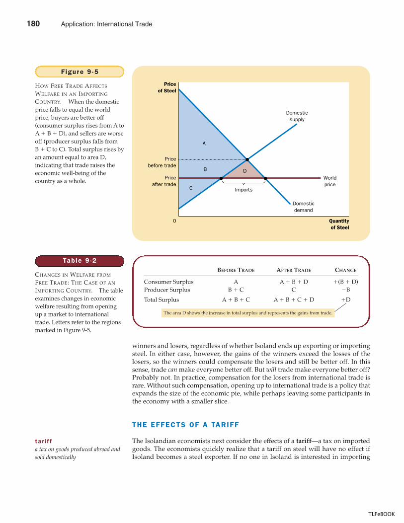
186 PART THREE SUPPLY AND DEMAND I I : MARKETS AND WELFARE
winners and losers, regardless of whether Isoland ends up exporting or importingsteel. In either case, however, the gains of the winners exceed the losses of thelosers, so the winners could compensate the losers and still be better off. In thissense, trade can make everyone better off. But will trade make everyone better off?Probably not. In practice, compensation for the losers from international trade israre. Without such compensation, opening up to international trade is a policy thatexpands the size of the economic pie, while perhaps leaving some participants inthe economy with a smaller slice.
THE EFFECTS OF A TARIFF
The Isolandian economists next consider the effects of a tariff—a tax on importedgoods. The economists quickly realize that a tariff on steel will have no effect ifIsoland becomes a steel exporter. If no one in Isoland is interested in importing
C
B D
A
Priceof Steel
Pricebefore trade
0 Quantityof Steel
Domesticsupply
Domesticdemand
Priceafter trade
Worldprice
Imports
Figure 9 -5
HOW FREE TRADE AFFECTS
WELFARE IN AN IMPORTING
COUNTRY. When the domesticprice falls to equal the worldprice, buyers are better off(consumer surplus rises from A toA � B � D), and sellers are worseoff (producer surplus falls fromB � C to C). Total surplus rises byan amount equal to area D,indicating that trade raises theeconomic well-being of thecountry as a whole.
Table 9 -2
CHANGES IN WELFARE FROM
FREE TRADE: THE CASE OF AN
IMPORTING COUNTRY. The tableexamines changes in economicwelfare resulting from openingup a market to internationaltrade. Letters refer to the regionsmarked in Figure 9-5.
BEFORE TRADE AFTER TRADE CHANGE
Consumer Surplus A A � B � D �(B � D)Producer Surplus B � C C �B
Total Surplus A � B � C A � B � C � D �D
tar i f fa tax on goods produced abroad andsold domestically
The area D shows the increase in total surplus and represents the gains from trade.
180 Application: International Trade
TLFeBOOK
CHAPTER 9 APPLICATION: INTERNATIONAL TRADE 187
steel, a tax on steel imports is irrelevant. The tariff matters only if Isoland becomesa steel importer. Concentrating their attention on this case, the economists com-pare welfare with and without the tariff.
Figure 9-6 shows the Isolandian market for steel. Under free trade, the domes-tic price equals the world price. A tariff raises the price of imported steel above theworld price by the amount of the tariff. Domestic suppliers of steel, who competewith suppliers of imported steel, can now sell their steel for the world price plusthe amount of the tariff. Thus, the price of steel—both imported and domestic—rises by the amount of the tariff and is, therefore, closer to the price that wouldprevail without trade.
The change in price affects the behavior of domestic buyers and sellers. Be-cause the tariff raises the price of steel, it reduces the domestic quantity demandedfrom Q1
D to Q2D and raises the domestic quantity supplied from Q1
S to Q2S. Thus, the
tariff reduces the quantity of imports and moves the domestic market closer to its equilib-rium without trade.
Now consider the gains and losses from the tariff. Because the tariff raises thedomestic price, domestic sellers are better off, and domestic buyers are worse off.In addition, the government raises revenue. To measure these gains and losses, welook at the changes in consumer surplus, producer surplus, and government rev-enue. These changes are summarized in Table 9-3.
Before the tariff, the domestic price equals the world price. Consumer surplus,the area between the demand curve and the world price, is area A � B � C � D �E � F. Producer surplus, the area between the supply curve and the world price,is area G. Government revenue equals zero. Total surplus, the sum of consumersurplus, producer surplus, and government revenue, is area A � B � C � D � E� F � G.
OUR STORY ABOUT THE STEEL INDUSTRY
and the debate over trade policy inIsoland is just a parable. Or is it?
C l i n t o n W a r n s U . S . W i l lF i g h t C h e a p I m p o r t s
BY DAVID E. SANGER
President Clinton said for the first timetoday that the United States would nottolerate the “flooding of our markets”with low-cost goods from Asia and Rus-sia, particularly steel, that are threaten-ing the jobs of American workers.
The President’s statement camedays after a White House meeting of topexecutives of steel companies and theUnited Steelworkers of America, whichhelped get out the vote for Democratslast week, playing a pivotal role withother unions in the party’s success inmidterm elections.
After the meeting, which includedMr. Clinton, Vice President Al Gore, andtop Cabinet officials, aides said theWhite House would not grant the unions’demand to cut off imports of steel theysay are being dumped in the Americanmarkets. But today, the Presidentwarned that foreign nations must “playby the rules,” appearing to signal thatthe United States would press other na-tions to restrict their exports to theUnited States. [Author’s note: In theend, the Clinton administration did de-cide to limit steel imports.]
SOURCE: The New York Times, November 11, 1998,p A1.
IN THE NEWS
Life in Isoland
Application: International Trade 181
TLFeBOOK
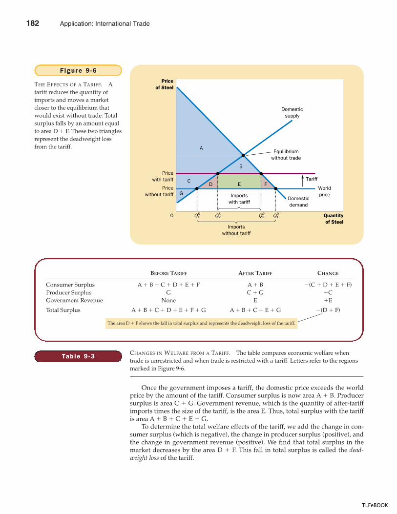
188 PART THREE SUPPLY AND DEMAND I I : MARKETS AND WELFARE
Once the government imposes a tariff, the domestic price exceeds the worldprice by the amount of the tariff. Consumer surplus is now area A � B. Producersurplus is area C � G. Government revenue, which is the quantity of after-tariffimports times the size of the tariff, is the area E. Thus, total surplus with the tariffis area A � B � C � E � G.
To determine the total welfare effects of the tariff, we add the change in con-sumer surplus (which is negative), the change in producer surplus (positive), andthe change in government revenue (positive). We find that total surplus in themarket decreases by the area D � F. This fall in total surplus is called the dead-weight loss of the tariff.
D E FC
G
B
A
Priceof Steel
0 Quantityof Steel
Domesticsupply
Domesticdemand
Pricewith tariff Tariff
Importswithout tariff
Equilibriumwithout trade
Pricewithout tariff
WorldpriceImports
with tariff
2QS1QS
2QD1QD
Figure 9 -6
THE EFFECTS OF A TARIFF. Atariff reduces the quantity ofimports and moves a marketcloser to the equilibrium thatwould exist without trade. Totalsurplus falls by an amount equalto area D � F. These two trianglesrepresent the deadweight lossfrom the tariff.
Table 9 -3
BEFORE TARIFF AFTER TARIFF CHANGE
Consumer Surplus A � B � C � D � E � F A � B �(C � D � E � F)Producer Surplus G C � G �CGovernment Revenue None E �E
Total Surplus A � B � C � D � E � F � G A � B � C � E � G �(D � F)
CHANGES IN WELFARE FROM A TARIFF. The table compares economic welfare whentrade is unrestricted and when trade is restricted with a tariff. Letters refer to the regionsmarked in Figure 9-6.
The area D � F shows the fall in total surplus and represents the deadweight loss of the tariff.
182 Application: International Trade
TLFeBOOK
CHAPTER 9 APPLICATION: INTERNATIONAL TRADE 189
It is not surprising that a tariff causes a deadweight loss, because a tariff is atype of tax. Like any tax on the sale of a good, it distorts incentives and pushes theallocation of scarce resources away from the optimum. In this case, we can identifytwo effects. First, the tariff on steel raises the price of steel that domestic producerscan charge above the world price and, as a result, encourages them to increase pro-duction of steel (from Q1
S to Q2S). Second, the tariff raises the price that domestic
steel buyers have to pay and, therefore, encourages them to reduce consumptionof steel (from Q1
D to Q2D). Area D represents the deadweight loss from the overpro-
duction of steel, and area F represents the deadweight loss from the undercon-sumption. The total deadweight loss of the tariff is the sum of these two triangles.
THE EFFECTS OF AN IMPORT QUOTA
The Isolandian economists next consider the effects of an import quota—a limit onthe quantity of imports. In particular, imagine that the Isolandian government dis-tributes a limited number of import licenses. Each license gives the license holderthe right to import 1 ton of steel into Isoland from abroad. The Isolandian econo-mists want to compare welfare under a policy of free trade and welfare with theaddition of this import quota.
Figure 9-7 shows how an import quota affects the Isolandian market for steel.Because the import quota prevents Isolandians from buying as much steel as theywant from abroad, the supply of steel is no longer perfectly elastic at the worldprice. Instead, as long as the price of steel in Isoland is above the world price, thelicense holders import as much as they are permitted, and the total supply of steelin Isoland equals the domestic supply plus the quota amount. That is, the supplycurve above the world price is shifted to the right by exactly the amount of thequota. (The supply curve below the world price does not shift because, in this case,importing is not profitable for the license holders.)
The price of steel in Isoland adjusts to balance supply (domestic plus im-ported) and demand. As the figure shows, the quota causes the price of steel to riseabove the world price. The domestic quantity demanded falls from Q1
D to Q2D, and
the domestic quantity supplied rises from Q1S to Q2
S. Not surprisingly, the importquota reduces steel imports.
Now consider the gains and losses from the quota. Because the quota raisesthe domestic price above the world price, domestic sellers are better off, and do-mestic buyers are worse off. In addition, the license holders are better off becausethey make a profit from buying at the world price and selling at the higherdomestic price. To measure these gains and losses, we look at the changes inconsumer surplus, producer surplus, and license-holder surplus, as shown inTable 9-4.
Before the government imposes the quota, the domestic price equals the worldprice. Consumer surplus, the area between the demand curve and the world price,is area A � B � C � D � E' � E''� F. Producer surplus, the area between the sup-ply curve and the world price, is area G. The surplus of license holders equals zerobecause there are no licenses. Total surplus, the sum of consumer, producer, andlicense-holder surplus, is area A � B � C � D � E' � E'' � F � G.
After the government imposes the import quota and issues the licenses, thedomestic price exceeds the world price. Domestic consumers get surplus equal toarea A � B, and domestic producers get surplus equal to area C � G. The licenseholders make a profit on each unit imported equal to the difference between the
impor t quotaa limit on the quantity of a good thatcan be produced abroad and solddomestically
Application: International Trade 183
TLFeBOOK
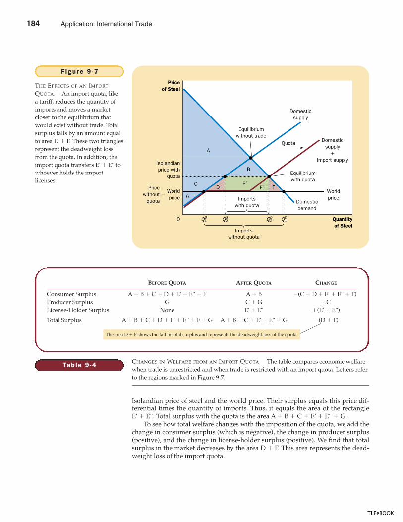
190 PART THREE SUPPLY AND DEMAND I I : MARKETS AND WELFARE
Isolandian price of steel and the world price. Their surplus equals this price dif-ferential times the quantity of imports. Thus, it equals the area of the rectangleE' � E''. Total surplus with the quota is the area A � B � C � E' � E'' � G.
To see how total welfare changes with the imposition of the quota, we add thechange in consumer surplus (which is negative), the change in producer surplus(positive), and the change in license-holder surplus (positive). We find that totalsurplus in the market decreases by the area D � F. This area represents the dead-weight loss of the import quota.
DE�
E� FC
G
B
A
Priceof Steel
0 Quantityof Steel
Domesticsupply
Domesticsupply
�
Import supply
Domesticdemand
Isolandianprice with
quota
Importswithout quota
Equilibriumwith quota
Equilibriumwithout trade
Quota
Worldprice
Pricewithout
quota
WorldpriceImports
with quota
2QS1QS
2QD1QD
�
Figure 9 -7
THE EFFECTS OF AN IMPORT
QUOTA. An import quota, likea tariff, reduces the quantity ofimports and moves a marketcloser to the equilibrium thatwould exist without trade. Totalsurplus falls by an amount equalto area D � F. These two trianglesrepresent the deadweight lossfrom the quota. In addition, theimport quota transfers E' � E'' towhoever holds the importlicenses.
Table 9 -4
BEFORE QUOTA AFTER QUOTA CHANGE
Consumer Surplus A � B � C � D � E' � E'' � F A � B �(C � D � E' � E'' � F)Producer Surplus G C � G �CLicense-Holder Surplus None E' � E'' �(E' � E'')
Total Surplus A � B � C � D � E' � E'' � F � G A � B � C � E' � E'' � G �(D � F)
CHANGES IN WELFARE FROM AN IMPORT QUOTA. The table compares economic welfarewhen trade is unrestricted and when trade is restricted with an import quota. Letters referto the regions marked in Figure 9-7.
The area D � F shows the fall in total surplus and represents the deadweight loss of the quota.
184 Application: International Trade
TLFeBOOK
CHAPTER 9 APPLICATION: INTERNATIONAL TRADE 191
This analysis should seem somewhat familiar. Indeed, if you compare theanalysis of import quotas in Figure 9-7 with the analysis of tariffs in Figure 9-6, youwill see that they are essentially identical. Both tariffs and import quotas raise the do-mestic price of the good, reduce the welfare of domestic consumers, increase the welfare ofdomestic producers, and cause deadweight losses. There is only one difference betweenthese two types of trade restriction: A tariff raises revenue for the government(area E in Figure 9-6), whereas an import quota creates surplus for license holders(area E' � E'' in Figure 9-7).
Tariffs and import quotas can be made to look even more similar. Suppose thatthe government tries to capture the license-holder surplus for itself by charging afee for the licenses. A license to sell 1 ton of steel is worth exactly the difference be-tween the Isolandian price of steel and the world price, and the government canset the license fee as high as this price differential. If the government does this, thelicense fee for imports works exactly like a tariff: Consumer surplus, producer sur-plus, and government revenue are exactly the same under the two policies.
In practice, however, countries that restrict trade with import quotas rarely doso by selling the import licenses. For example, the U.S. government has at timespressured Japan to “voluntarily” limit the sale of Japanese cars in the UnitedStates. In this case, the Japanese government allocates the import licenses to Japan-ese firms, and the surplus from these licenses (area E' � E'') accrues to those firms.This kind of import quota is, from the standpoint of U.S. welfare, strictly worsethan a U.S. tariff on imported cars. Both a tariff and an import quota raise prices,restrict trade, and cause deadweight losses, but at least the tariff produces revenuefor the U.S. government rather than for Japanese auto companies.
Although in our analysis so far import quotas and tariffs appear to cause sim-ilar deadweight losses, a quota can potentially cause an even larger deadweightloss, depending on the mechanism used to allocate the import licenses. Supposethat when Isoland imposes a quota, everyone understands that the licenses will goto those who spend the most resources lobbying the Isolandian government. Inthis case, there is an implicit license fee—the cost of lobbying. The revenues fromthis fee, however, rather than being collected by the government, are spent on lob-bying expenses. The deadweight losses from this type of quota include not onlythe losses from overproduction (area D) and underconsumption (area F) but alsowhatever part of the license-holder surplus (area E'�E'') is wasted on the cost oflobbying.
THE LESSONS FOR TRADE POLICY
The team of Isolandian economists can now write to the new president:
Dear Madam President,
You asked us three questions about opening up trade. After muchhard work, we have the answers.
Question: If the government allowed Isolandians to import and exportsteel, what would happen to the price of steel and the quantity of steelsold in the domestic steel market?
Answer: Once trade is allowed, the Isolandian price of steel would bedriven to equal the price prevailing around the world.
Application: International Trade 185
TLFeBOOK
192 PART THREE SUPPLY AND DEMAND I I : MARKETS AND WELFARE
If the world price is now higher than the Isolandian price, our pricewould rise. The higher price would reduce the amount of steel Isolandiansconsume and raise the amount of steel that Isolandians produce. Isolandwould, therefore, become a steel exporter. This occurs because, in this case,Isoland would have a comparative advantage in producing steel.
Conversely, if the world price is now lower than the Isolandian price,our price would fall. The lower price would raise the amount of steel thatIsolandians consume and lower the amount of steel that Isolandians pro-duce. Isoland would, therefore, become a steel importer. This occurs be-cause, in this case, other countries would have a comparative advantagein producing steel.
Question: Who would gain from free trade in steel and who wouldlose, and would the gains exceed the losses?
Answer: The answer depends on whether the price rises or falls whentrade is allowed. If the price rises, producers of steel gain, and consumersof steel lose. If the price falls, consumers gain, and producers lose. In bothcases, the gains are larger than the losses. Thus, free trade raises the totalwelfare of Isolandians.
Question: Should a tariff or an import quota be part of the new tradepolicy?
Answer: A tariff, like most taxes, has deadweight losses: The revenueraised would be smaller than the losses to the buyers and sellers. In thiscase, the deadweight losses occur because the tariff would move the econ-omy closer to our current no-trade equilibrium. An import quota worksmuch like a tariff and would cause similar deadweight losses. The bestpolicy, from the standpoint of economic efficiency, would be to allow tradewithout a tariff or an import quota.
We hope you find these answers helpful as you decide on your newpolicy.
Your faithful servants,Isolandian economics team
QUICK QUIZ: Draw the supply and demand curve for wool suits in the country of Autarka. When trade is allowed, the price of a suit falls from 3 to 2 ounces of gold. In your diagram, what is the change in consumer surplus, the change in producer surplus, and the change in total surplus? How would a tariff on suit imports alter these effects?
THE ARGUMENTS FOR RESTRICTING TRADE
The letter from the economics team persuades the new president of Isoland to con-sider opening up trade in steel. She notes that the domestic price is now high com-pared to the world price. Free trade would, therefore, cause the price of steel to falland hurt domestic steel producers. Before implementing the new policy, she asksIsolandian steel companies to comment on the economists’ advice.
186 Application: International Trade
TLFeBOOK
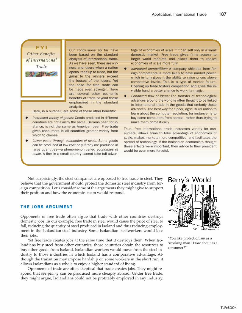
CHAPTER 9 APPLICATION: INTERNATIONAL TRADE 193
Not surprisingly, the steel companies are opposed to free trade in steel. Theybelieve that the government should protect the domestic steel industry from for-eign competition. Let’s consider some of the arguments they might give to supporttheir position and how the economics team would respond.
THE JOBS ARGUMENT
Opponents of free trade often argue that trade with other countries destroysdomestic jobs. In our example, free trade in steel would cause the price of steel tofall, reducing the quantity of steel produced in Isoland and thus reducing employ-ment in the Isolandian steel industry. Some Isolandian steelworkers would losetheir jobs.
Yet free trade creates jobs at the same time that it destroys them. When Iso-landians buy steel from other countries, those countries obtain the resources tobuy other goods from Isoland. Isolandian workers would move from the steel in-dustry to those industries in which Isoland has a comparative advantage. Al-though the transition may impose hardship on some workers in the short run, itallows Isolandians as a whole to enjoy a higher standard of living.
Opponents of trade are often skeptical that trade creates jobs. They might re-spond that everything can be produced more cheaply abroad. Under free trade,they might argue, Isolandians could not be profitably employed in any industry.
Our conclusions so far havebeen based on the standardanalysis of international trade.As we have seen, there are win-ners and losers when a nationopens itself up to trade, but thegains to the winners exceedthe losses of the losers. Yetthe case for free trade canbe made even stronger. Thereare several other economicbenefits of trade beyond thoseemphasized in the standardanalysis.
Here, in a nutshell, are some of these other benefits:
� Increased variety of goods: Goods produced in differentcountries are not exactly the same. German beer, for in-stance, is not the same as American beer. Free tradegives consumers in all countries greater variety fromwhich to choose.
� Lower costs through economies of scale: Some goodscan be produced at low cost only if they are produced inlarge quantities—a phenomenon called economies ofscale. A firm in a small country cannot take full advan-
tage of economies of scale if it can sell only in a smalldomestic market. Free trade gives firms access tolarger world markets and allows them to realizeeconomies of scale more fully.
� Increased competition: A company shielded from for-eign competitors is more likely to have market power,which in turn gives it the ability to raise prices abovecompetitive levels. This is a type of market failure.Opening up trade fosters competition and gives the in-visible hand a better chance to work its magic.
� Enhanced flow of ideas: The transfer of technologicaladvances around the world is often thought to be linkedto international trade in the goods that embody thoseadvances. The best way for a poor, agricultural nation tolearn about the computer revolution, for instance, is tobuy some computers from abroad, rather than trying tomake them domestically.
Thus, free international trade increases variety for con-sumers, allows firms to take advantage of economies ofscale, makes markets more competitive, and facilitates thespread of technology. If the Isolandian economists thoughtthese effects were important, their advice to their presidentwould be even more forceful.
FYI
Other Benefitsof International
Trade
“You like protectionism as a‘working man.’ How about as aconsumer?”
Application: International Trade 187
TLFeBOOK
194 PART THREE SUPPLY AND DEMAND I I : MARKETS AND WELFARE
As Chapter 3 explains, however, the gains from trade are based on comparativeadvantage, not absolute advantage. Even if one country is better than anothercountry at producing everything, each country can still gain from trading with theother. Workers in each country will eventually find jobs in the industry in whichthat country has a comparative advantage.
THE NATIONAL-SECURITY ARGUMENT
When an industry is threatened with competition from other countries, opponentsof free trade often argue that the industry is vital for national security. In our ex-ample, Isolandian steel companies might point out that steel is used to make gunsand tanks. Free trade would allow Isoland to become dependent on foreign coun-tries to supply steel. If a war later broke out, Isoland might be unable to produceenough steel and weapons to defend itself.
Economists acknowledge that protecting key industries may be appropriatewhen there are legitimate concerns over national security. Yet they fear that this ar-gument may be used too quickly by producers eager to gain at consumers’ ex-pense. The U.S. watchmaking industry, for instance, long argued that it was vitalfor national security, claiming that its skilled workers would be necessary inwartime. Certainly, it is tempting for those in an industry to exaggerate their rolein national defense in order to obtain protection from foreign competition.
THE INFANT- INDUSTRY ARGUMENT
New industries sometimes argue for temporary trade restrictions to help them getstarted. After a period of protection, the argument goes, these industries will ma-ture and be able to compete with foreign competitors. Similarly, older industriessometimes argue that they need temporary protection to help them adjust to newconditions. For example, General Motors Chairman Roger Smith once argued fortemporary protection “to give U.S. automakers turnaround time to get the domes-tic industry back on its feet.”
Economists are often skeptical about such claims. The primary reason is thatthe infant-industry argument is difficult to implement in practice. To apply pro-tection successfully, the government would need to decide which industries willeventually be profitable and decide whether the benefits of establishing these in-dustries exceed the costs to consumers of protection. Yet “picking winners” is ex-traordinarily difficult. It is made even more difficult by the political process, whichoften awards protection to those industries that are politically powerful. And oncea powerful industry is protected from foreign competition, the “temporary” policyis hard to remove.
In addition, many economists are skeptical about the infant-industry argu-ment even in principle. Suppose, for instance, that the Isolandian steel industry isyoung and unable to compete profitably against foreign rivals. Yet there is reasonto believe that the industry can be profitable in the long run. In this case, the own-ers of the firms should be willing to incur temporary losses in order to obtain theeventual profits. Protection is not necessary for an industry to grow. Firms in var-ious industries—such as many Internet firms today—incur temporary losses in thehope of growing and becoming profitable in the future. And many of them suc-ceed, even without protection from foreign competition.
188 Application: International Trade
TLFeBOOK
CHAPTER 9 APPLICATION: INTERNATIONAL TRADE 195
CASE STUDY TRADE AGREEMENTS
A country can take one of two approaches to achieving free trade. It can take aunilateral approach and remove its trade restrictions on its own. This is the ap-proach that Great Britain took in the nineteenth century and that Chile andSouth Korea have taken in recent years. Alternatively, a country can take a mul-tilateral approach and reduce its trade restrictions while other countries do the
THE UNFAIR -COMPETIT ION ARGUMENT
A common argument is that free trade is desirable only if all countries play by thesame rules. If firms in different countries are subject to different laws and regu-lations, then it is unfair (the argument goes) to expect the firms to compete in theinternational marketplace. For instance, suppose that the government of Neigh-borland subsidizes its steel industry by giving steel companies large tax breaks.The Isolandian steel industry might argue that it should be protected from this for-eign competition because Neighborland is not competing fairly.
Would it, in fact, hurt Isoland to buy steel from another country at a sub-sidized price? Certainly, Isolandian steel producers would suffer, but Isolandiansteel consumers would benefit from the low price. Moreover, the case for free tradeis no different: The gains of the consumers from buying at the low price would ex-ceed the losses of the producers. Neighborland’s subsidy to its steel industry maybe a bad policy, but it is the taxpayers of Neighborland who bear the burden.Isoland can benefit from the opportunity to buy steel at a subsidized price.
THE PROTECTION-AS-A -BARGAINING-CHIP ARGUMENT
Another argument for trade restrictions concerns the strategy of bargaining. Manypolicymakers claim to support free trade but, at the same time, argue that trade re-strictions can be useful when we bargain with our trading partners. They claimthat the threat of a trade restriction can help remove a trade restriction already im-posed by a foreign government. For example, Isoland might threaten to impose atariff on steel unless Neighborland removes its tariff on wheat. If Neighborland re-sponds to this threat by removing its tariff, the result can be freer trade.
The problem with this bargaining strategy is that the threat may not work. If itdoesn’t work, the country has a difficult choice. It can carry out its threat and im-plement the trade restriction, which would reduce its own economic welfare. Or itcan back down from its threat, which would cause it to lose prestige in interna-tional affairs. Faced with this choice, the country would probably wish that it hadnever made the threat in the first place.
An example of this occurred in 1999, when the U.S. government accusedEuropeans of restricting the import of U.S. bananas. After a long and bitter disputewith governments that are normally U.S. allies, the United States placed 100 per-cent tariffs on a range of European products from cheese to cashmere. In the end,not only were Europeans denied the benefits of American bananas, but Americanswere denied the benefits of European cheese. Sometimes, when a government en-gages in a game of brinkmanship, as the United States did in this case, everyonegoes over the brink together.
Application: International Trade 189
TLFeBOOK
196 PART THREE SUPPLY AND DEMAND I I : MARKETS AND WELFARE
same. In other words, it can bargain with its trading partners in an attempt toreduce trade restrictions around the world.
One important example of the multilateral approach is the North AmericanFree Trade Agreement (NAFTA), which in 1993 lowered trade barriers amongthe United States, Mexico, and Canada. Another is the General Agreement on
WHEN DOMESTIC PRODUCERS COMPLAIN
about competition from abroad, theyoften assert that consumers are not wellserved by imperfect foreign products.The following article documents howRussian producers of chicken reacted tocompetition from the United States.
U . S . C h i c k e n i n E v e r y P o t ?N y e t ! R u s s i a n s C r y F o u l
BY MICHAEL R. GORDON
Moscow—A nasty little skirmish be-tween Russia and the United States isbrewing here over a threatened tradebarrier.
But this fight is not about manufac-tured consumer goods or high technol-ogy, but about American chicken, whichhas flooded the Russian market.
To the frustration, and considerableanxiety, of American companies, theRussian government has threatened toban further American poultry sales effec-tive March 19. . . .
The ostensible reason for the Rus-sian government’s warning is health—a
seemingly strange concern in a countrywith a generally lax record in observingsafety standards, where virtually everyable-bodied man and woman smokes.
Today, no less an authority than theVeterinary Department of the RussianAgriculture and Food Ministry said theban was needed to protect consumershere against infected poultry until theUnited States improved its standards.
But the real agenda, Americanproducers contend, is old-fashionedprotectionism.
Agitated Russian producers, whosebirds, Russian consumers say, are nomatch for their American competition interms of quality and price, have repeat-edly complained that the United Statesis trying to destroy the Russian poultryindustry and capture its market. And nowAmerican companies fear the Russianproducers are striking back. . . .
The first big invasion of frozen poul-try [into Russia] came during the Bushadministration. . . . The export provedto be very popular with Russian con-sumers, who dubbed them Bush legs.
After the demise of the SovietUnion, American poultry exports con-tinued to soar. Russian poultry produc-tion, meanwhile, fell 40 percent, theresult of rising grain prices and decliningsubsidies.
Astoundingly, a third of all Americanexports to Russia is poultry, Americanofficials say. . . .
If the confrontation continues, theUnited States has a number of possible
recourses, including arguing that theRussian action is inconsistent withMoscow’s bid to join the World TradeOrganization.
Some experts, however, believethere is an important countervailing forcehere that may lead to a softening ofthe Russian position: namely Russianconsumers.
Russian consumers favor the Amer-ican birds, which despite the dire warn-ings of the Russian government, havecome to symbolize quality. And theyvote, too.
SOURCE: The New York Times, February 24, 1996,pp. 33, 34.
IN THE NEWS
A Chicken Invasion
A THREAT TO RUSSIA?
190 Application: International Trade
TLFeBOOK
CHAPTER 9 APPLICATION: INTERNATIONAL TRADE 197
Tariffs and Trade (GATT), which is a continuing series of negotiations amongmany of the world’s countries with the goal of promoting free trade. The UnitedStates helped to found GATT after World War II in response to the high tariffsimposed during the Great Depression of the 1930s. Many economists believethat the high tariffs contributed to the economic hardship during that period.GATT has successfully reduced the average tariff among member countriesfrom about 40 percent after World War II to about 5 percent today. The rules es-tablished under GATT are now enforced by an international institution calledthe World Trade Organization (WTO).
What are the pros and cons of the multilateral approach to free trade? Oneadvantage is that the multilateral approach has the potential to result in freertrade than a unilateral approach because it can reduce trade restrictions abroadas well as at home. If international negotiations fail, however, the result couldbe more restricted trade than under a unilateral approach.
In addition, the multilateral approach may have a political advantage. Inmost markets, producers are fewer and better organized than consumers—andthus wield greater political influence. Reducing the Isolandian tariff on steel, forexample, may be politically difficult if considered by itself. The steel companieswould oppose free trade, and the users of steel who would benefit are so nu-merous that organizing their support would be difficult. Yet suppose thatNeighborland promises to reduce its tariff on wheat at the same time thatIsoland reduces its tariff on steel. In this case, the Isolandian wheat farmers,who are also politically powerful, would back the agreement. Thus, the multi-lateral approach to free trade can sometimes win political support when a uni-lateral reduction cannot.
QUICK QUIZ: The textile industry of Autarka advocates a ban on the import of wool suits. Describe five arguments its lobbyists might make. Give a response to each of these arguments.
CONCLUSION
Economists and the general public often disagree about free trade. In 1993, for ex-ample, the United States faced the question of whether to ratify the North Ameri-can Free Trade Agreement, which reduced trade restrictions among the UnitedStates, Canada, and Mexico. Opinion polls showed the general public in theUnited States about evenly split on the issue, and the agreement passed in Con-gress by only a narrow margin. Opponents viewed free trade as a threat to jobsecurity and the American standard of living. By contrast, economists overwhelm-ingly supported the agreement. They viewed free trade as a way of allocating pro-duction efficiently and raising living standards in all three countries.
Economists view the United States as an ongoing experiment that confirms thevirtues of free trade. Throughout its history, the United States has allowed unre-stricted trade among the states, and the country as a whole has benefited from thespecialization that trade allows. Florida grows oranges, Texas pumps oil, Califor-nia makes wine, and so on. Americans would not enjoy the high standard of living
Application: International Trade 191
TLFeBOOK
198 PART THREE SUPPLY AND DEMAND I I : MARKETS AND WELFARE
they do today if people could consume only those goods and services producedin their own states. The world could similarly benefit from free trade amongcountries.
To better understand economists’ view of trade, let’s continue our parable.Suppose that the country of Isoland ignores the advice of its economics team anddecides not to allow free trade in steel. The country remains in the equilibriumwithout international trade.
Then, one day, some Isolandian inventor discovers a new way to make steel atvery low cost. The process is quite mysterious, however, and the inventor insistson keeping it a secret. What is odd is that the inventor doesn’t need any workersor iron ore to make steel. The only input he requires is wheat.
ECONOMIST JAGDISH BHAGWATI ARGUES
that the United States should lower itstrade barriers unilaterally.
F r e e Tr a d e w i t h o u t Tr e a t i e s
BY JAGDISH BHAGWATI
President Clinton and 17 other Asian-Pacific leaders are meeting today inVancouver. Rather than the convivialphoto-op they’d planned, however, theymust contend with worrisome tradenews. A spate of Asian currency devalu-ations has raised the specter of renewedprotectionism around the world. SouthAmerica’s Mercosur trade bloc, led byBrazil, just raised its tariffs some 30 per-cent. And Congress turned its back onthe president and refused to approvefast-track authority for him to negotiatefurther free-trade accords. [Author’s
note: Fast-track authority would allowthe president to negotiate trade dealsthat Congress would consider withoutthe ability to attach amendments.]
In light of all this dismaying news,what are the prospects for free trade? Isthe future bleak, or will the postwar trendof dramatic liberalization continue to ac-celerate despite these setbacks?
The immediate prospects for moreU.S.-led multilateral trade accords do in-deed look grim after the defeat of fast-track. But that doesn’t mean that freetrade itself is on the ropes. A large por-tion of the world’s trade liberalization inthe last quarter-century has been unilat-eral. Those countries that lower tradebarriers of their own accord not onlyprofit themselves, but also often inducethe laggards to match their example. Themost potent force for the worldwidefreeing of trade, then, is unilateral U.S.action. If the United States continues todo away with tariffs and trade barriers,other countries will follow suit—fast-track or no fast-track.
To be sure, the General Agreementon Tariffs and Trade, the World Trade Or-ganization, and other multilateral tariff re-ductions have greatly contributed toglobal wealth. The WTO has become theinternational institution for setting the“rules” on public and private practices
that affect competition among tradingnations. Much still needs to be done inthat mode, particularly on agriculture tar-iffs, which remain too high around theworld. A future U.S. president, if not Mr.Clinton, will certainly need fast-track au-thority if another multilateral effort, suchas the “millennium round” called for bySir Leon Brittan of the European Union,is to pursue these goals.
But the good news is that even iforganized labor, radical environmental-ists, and others who fear the globaleconomy continue to impede fast-trackduring Congress’s next session, theycannot stop the historic freeing of tradethat has been occurring unilaterallyworldwide.
From the 1970s through the 1990s,Latin America witnessed dramatic lower-ing of trade barriers unilaterally by Chile,Bolivia, and Paraguay; and the entirecontinent has been moving steadily to-ward further trade liberalization. Merco-sur’s recent actions are a setback, butonly a small one—so far.
Latin America’s record has beenbettered by unilateral liberalizers in Asiaand the Pacific. New Zealand began dis-mantling its substantial trade protectionapparatus in 1985. That effort was drivenby the reformist views of then-PrimeMinister David Lange, who declared, “In
IN THE NEWSThe Case for
Unilateral Disarmamentin the Trade Wars
192 Application: International Trade
TLFeBOOK
CHAPTER 9 APPLICATION: INTERNATIONAL TRADE 199
The inventor is hailed as a genius. Because steel is used in so many products,the invention lowers the cost of many goods and allows all Isolandians to enjoy ahigher standard of living. Workers who had previously produced steel do sufferwhen their factories close, but eventually they find work in other industries. Somebecome farmers and grow the wheat that the inventor turns into steel. Others en-ter new industries that emerge as a result of higher Isolandian living standards.Everyone understands that the displacement of these workers is an inevitable partof progress.
After several years, a newspaper reporter decides to investigate this mysteri-ous new steel process. She sneaks into the inventor’s factory and learns that the in-ventor is a fraud. The inventor has not been making steel at all. Instead, he has
the course of about three years wechanged from being a country run like aPolish shipyard into one that could be in-ternationally competitive.”
Since the 1980s, Hong Kong’s andSingapore’s enormous successes asfree traders have served as potent ex-amples of unilateral market opening, en-couraging Indonesia, the Philippines,Thailand, South Korea, and Malaysia tofollow suit. By 1991 even India, whichhas been astonishingly autarkic for morethan four decades, had finally learned thevirtue of free trade and had embarked ona massive lowering of its tariffs and non-tariff barriers.
In Central and Eastern Europe, thecollapse of communism led to a whole-sale, unilateral, and nondiscriminatory re-moval of trade barriers as well. TheFrench economist Patrick Messerlin hasshown how this happened in threewaves: Czechoslovakia, Poland, andHungary liberalized right after the fall ofthe Berlin Wall; next came Bulgaria, Ro-mania, and Slovenia; and finally, theBaltic countries began unilateral openingin 1991. . . .
U.S. leadership is crucial to main-taining the trend toward free trade. Suchultramodern industries as telecommuni-cations and financial services gainedtheir momentum largely from unilateral
openness and deregulation in the UnitedStates. This in turn led to a softening ofprotectionist attitudes in the EuropeanUnion and Japan.
These developed economies arenow moving steadily in the direction ofopenness and competition—not be-cause any officials in Washingtonthreaten them with retribution, but be-cause they’ve seen how U.S. companiesbecome more competitive once regula-tion and other trade barriers have fallen.A Brussels bureaucrat can argue with aWashington bureaucrat, but he cannotargue with the markets. Faced with theprospect of being elbowed out of worldmarkets by American firms, Japan andEurope have no option but to follow theU.S. example, belatedly but surely, inopening their own markets.
The biggest threat to free trade isnot the loss of fast-track per se, but thesignal it sends that Americans may notbe interested in lowering their trade bar-riers any further. To counteract this atti-tude, President Clinton needs to mountthe bully pulpit and explain the case forfree trade—a case that Adam Smith firstmade more than 200 years ago, but thatcontinues to come under attack.
The president, free from the bur-dens of constituency interests that crip-ple many in Congress, could argue,
credibly and with much evidence, thatfree trade is in the interest of the wholeworld, but that, because the U.S. econ-omy is the most competitive anywhere,we have the most to gain. The presidentcould also point to plenty of evidencethat debunks the claims of protection-ists. The unions may argue that tradewith poor countries depresses our work-ers’ wages, for example, but in fact thebest evidence shows that such trade hashelped workers by moderating the fall intheir wages from technological changes.
Assuming that the president canmake the case for free trade at home,the prospects for free trade worldwideremain bright. The United States doesn’tneed to sign treaties to open markets or,heaven forbid, issue counterproductivethreats to close our own markets if oth-ers are less open than we are. We sim-ply need to offer an example ofopenness and deregulation to the rest ofthe world. Other countries will see oursuccess, and seek to emulate it.
SOURCE: The Wall Street Journal, November 24,1997, p. A22.
Application: International Trade 193
TLFeBOOK
200 PART THREE SUPPLY AND DEMAND I I : MARKETS AND WELFARE
been smuggling wheat abroad in exchange for steel from other countries. The onlything that the inventor had discovered was the gains from international trade.
When the truth is revealed, the government shuts down the inventor’s opera-tion. The price of steel rises, and workers return to jobs in steel factories. Livingstandards in Isoland fall back to their former levels. The inventor is jailed and heldup to public ridicule. After all, he was no inventor. He was just an economist.
� The effects of free trade can be determined bycomparing the domestic price without trade to theworld price. A low domestic price indicates that thecountry has a comparative advantage in producing thegood and that the country will become an exporter. Ahigh domestic price indicates that the rest of the worldhas a comparative advantage in producing the good andthat the country will become an importer.
� When a country allows trade and becomes an exporterof a good, producers of the good are better off, andconsumers of the good are worse off. When a countryallows trade and becomes an importer of a good,consumers are better off, and producers are worse off. Inboth cases, the gains from trade exceed the losses.
� A tariff—a tax on imports—moves a market closer to theequilibrium that would exist without trade and,
therefore, reduces the gains from trade. Althoughdomestic producers are better off and the governmentraises revenue, the losses to consumers exceed thesegains.
� An import quota has effects that are similar to those of atariff. Under a quota, however, the holders of the importlicenses receive the revenue that the government wouldcollect with a tariff.
� There are various arguments for restricting trade:protecting jobs, defending national security, helpinginfant industries, preventing unfair competition, andresponding to foreign trade restrictions. Although someof these arguments have some merit in some cases,economists believe that free trade is usually the betterpolicy.
Summar y
world price, p. 181 tariff, p. 186 import quota, p. 189
Key Concepts
1. What does the domestic price that prevails withoutinternational trade tell us about a nation’s comparativeadvantage?
2. When does a country become an exporter of a good? Animporter?
3. Draw the supply-and-demand diagram for animporting country. What is consumer surplus andproducer surplus before trade is allowed? What isconsumer surplus and producer surplus with free trade?What is the change in total surplus?
4. Describe what a tariff is, and describe its economiceffects.
5. What is an import quota? Compare its economic effectswith those of a tariff.
6. List five arguments often given to support traderestrictions. How do economists respond to thesearguments?
7. What is the difference between the unilateral andmultilateral approaches to achieving free trade? Give anexample of each.
Quest ions fo r Rev iew
194 Application: International Trade
TLFeBOOK
CHAPTER 9 APPLICATION: INTERNATIONAL TRADE 201
1. The United States represents a small part of the worldorange market.a. Draw a diagram depicting the equilibrium in the
U.S. orange market without international trade.Identify the equilibrium price, equilibrium quantity,consumer surplus, and producer surplus.
b. Suppose that the world orange price is below theU.S. price before trade, and that the U.S. orangemarket is now opened to trade. Identify the newequilibrium price, quantity consumed, quantityproduced domestically, and quantity imported.Also show the change in the surplus of domesticconsumers and producers. Has domestic totalsurplus increased or decreased?
2. The world price of wine is below the price that wouldprevail in the United States in the absence of trade.a. Assuming that American imports of wine are a
small part of total world wine production, draw agraph for the U.S. market for wine under free trade.Identify consumer surplus, producer surplus, andtotal surplus in an appropriate table.
b. Now suppose that an unusual shift of the GulfStream leads to an unseasonably cold summer inEurope, destroying much of the grape harvestthere. What effect does this shock have on theworld price of wine? Using your graph and tablefrom part (a), show the effect on consumer surplus,producer surplus, and total surplus in the UnitedStates. Who are the winners and losers? Is theUnited States as a whole better or worse off?
3. The world price of cotton is below the no-trade price inCountry A and above the no-trade price in Country B.Using supply-and-demand diagrams and welfare tablessuch as those in the chapter, show the gains from tradein each country. Compare your results for the twocountries.
4. Suppose that Congress imposes a tariff on importedautos to protect the U.S. auto industry from foreigncompetition. Assuming that the U.S. is a price taker inthe world auto market, show on a diagram: the changein the quantity of imports, the loss to U.S. consumers,the gain to U.S. manufacturers, government revenue,and the deadweight loss associated with the tariff. Theloss to consumers can be decomposed into three pieces:a transfer to domestic producers, a transfer to thegovernment, and a deadweight loss. Use your diagramto identify these three pieces.
5. According to an article in The New York Times (Nov. 5,1993), “many Midwest wheat farmers oppose the [NorthAmerican] free trade agreement [NAFTA] as much asmany corn farmers support it.” For simplicity, assumethat the United States is a small country in the marketsfor both corn and wheat, and that without the free tradeagreement, the United States would not trade thesecommodities internationally. (Both of these assumptionsare false, but they do not affect the qualitative responsesto the following questions.)a. Based on this report, do you think the world wheat
price is above or below the U.S. no-trade wheatprice? Do you think the world corn price is aboveor below the U.S. no-trade corn price? Now analyzethe welfare consequences of NAFTA in bothmarkets.
b. Considering both markets together, does NAFTAmake U.S. farmers as a group better or worse off?Does it make U.S. consumers as a group better orworse off? Does it make the United States as awhole better or worse off?
6. Imagine that winemakers in the state of Washingtonpetitioned the state government to tax wines importedfrom California. They argue that this tax would bothraise tax revenue for the state government and raiseemployment in the Washington state wine industry. Doyou agree with these claims? Is it a good policy?
7. Senator Ernest Hollings once wrote that “consumers donot benefit from lower-priced imports. Glance throughsome mail-order catalogs and you’ll see that consumerspay exactly the same price for clothing whether it isU.S.-made or imported.” Comment.
8. Write a brief essay advocating or criticizing each of thefollowing policy positions:a. The government should not allow imports
if foreign firms are selling below their costsof production (a phenomenon called “dumping”).
b. The government should temporarily stop theimport of goods for which the domestic industry isnew and struggling to survive.
c. The government should not allow imports fromcountries with weaker environmental regulationsthan ours.
9. Suppose that a technological advance in Japan lowersthe world price of televisions.
Prob lems and App l icat ions
Application: International Trade 195
TLFeBOOK
202 PART THREE SUPPLY AND DEMAND I I : MARKETS AND WELFARE
a. Assume the U.S. is an importer of televisions andthere are no trade restrictions. How does thetechnological advance affect the welfare of U.S.consumers and U.S. producers? What happens tototal surplus in the United States?
b. Now suppose the United States has a quota ontelevision imports. How does the Japanesetechnological advance affect the welfare of U.S.consumers, U.S. producers, and the holders ofimport licenses?
10. When the government of Tradeland decides to imposean import quota on foreign cars, three proposals aresuggested: (1) Sell the import licenses in an auction.(2) Distribute the licenses randomly in a lottery. (3) Letpeople wait in line and distribute the licenses on a first-come, first-served basis. Compare the effects of thesepolicies. Which policy do you think has the largestdeadweight losses? Which policy has the smallestdeadweight losses? Why? (Hint: The government’sother ways of raising tax revenue all cause deadweightlosses themselves.)
11. An article in The Wall Street Journal (June 26, 1990) aboutsugar beet growers explained that “the governmentprops up domestic sugar prices by curtailing imports oflower-cost sugar. Producers are guaranteed a ‘marketstabilization price’ of $0.22 a pound, about $0.09 higherthan the current world market price.” The governmentmaintains the higher price by imposing an importquota.a. Illustrate the effect of this quota on the U.S. sugar
market. Label the relevant prices and quantitiesunder free trade and under the quota.
b. Analyze the effects of the sugar quota using thetools of welfare analysis.
c. The article also comments that “critics of the sugarprogram say that [the quota] has deprivednumerous sugar-producing nations in theCaribbean, Latin America, and Far East of exportearnings, harmed their economies, and causedpolitical instability, while increasing Third Worlddemand for U.S. foreign aid.” Our usual welfareanalysis includes only gains and losses to U.S.consumers and producers. What role do you thinkthe gains or losses to people in other countriesshould play in our economic policymaking?
d. The article continues that “at home, the sugarprogram has helped make possible the spectacularrise of the high-fructose corn syrup industry.” Whyhas the sugar program had this effect? (Hint: Aresugar and corn syrup substitutes or complements?)
12. (This question is challenging.) Consider a small countrythat exports steel. Suppose that a “pro-trade”government decides to subsidize the export of steel bypaying a certain amount for each ton sold abroad. Howdoes this export subsidy affect the domestic price ofsteel, the quantity of steel produced, the quantity ofsteel consumed, and the quantity of steel exported?How does it affect consumer surplus, producer surplus,government revenue, and total surplus? (Hint: Theanalysis of an export subsidy is similar to the analysis ofa tariff.)
196 Application: International Trade
TLFeBOOK
IN THIS CHAPTERYOU WILL . . .
Examine the variousgovernment pol iciesaimed at solving the
problem ofexternal it ies
Examine how peoplecan sometimes solve
the problem ofexternal it ies on
their own
Learn the nature ofan external ity
See whyexternal it ies can
make marketoutcomes inef f icient
Consider why privatesolutions toexternal it ies
sometimes do notwork
Firms that make and sell paper also create, as a by-product of the manufacturingprocess, a chemical called dioxin. Scientists believe that once dioxin enters the en-vironment, it raises the population’s risk of cancer, birth defects, and other healthproblems.
Is the production and release of dioxin a problem for society? In Chapters 4through 9 we examined how markets allocate scarce resources with the forces ofsupply and demand, and we saw that the equilibrium of supply and demand istypically an efficient allocation of resources. To use Adam Smith’s famousmetaphor, the “invisible hand” of the marketplace leads self-interested buyers andsellers in a market to maximize the total benefit that society derives from that mar-ket. This insight is the basis for one of the Ten Principles of Economics in Chapter 1:Markets are usually a good way to organize economic activity. Should we con-clude, therefore, that the invisible hand prevents firms in the paper market fromemitting too much dioxin?
E X T E R N A L I T I E S
205
197
10
TLFeBOOK
206 PART FOUR THE ECONOMICS OF THE PUBLIC SECTOR
Markets do many things well, but they do not do everything well. In this chap-ter we begin our study of another of the Ten Principles of Economics: Governmentscan sometimes improve market outcomes. We examine why markets sometimesfail to allocate resources efficiently, how government policies can potentially im-prove the market’s allocation, and what kinds of policies are likely to work best.
The market failures examined in this chapter fall under a general categorycalled externalities. An externality arises when a person engages in an activity thatinfluences the well-being of a bystander and yet neither pays nor receives anycompensation for that effect. If the impact on the bystander is adverse, it is calleda negative externality; if it is beneficial, it is called a positive externality. In the pres-ence of externalities, society’s interest in a market outcome extends beyond thewell-being of buyers and sellers in the market; it also includes the well-being of by-standers who are affected. Because buyers and sellers neglect the external effectsof their actions when deciding how much to demand or supply, the market equi-librium is not efficient when there are externalities. That is, the equilibrium fails tomaximize the total benefit to society as a whole. The release of dioxin into theenvironment, for instance, is a negative externality. Self-interested paper firms willnot consider the full cost of the pollution they create and, therefore, will emittoo much pollution unless the government prevents or discourages them fromdoing so.
Externalities come in many varieties, as do the policy responses that try to dealwith the market failure. Here are some examples:
� The exhaust from automobiles is a negative externality because it createssmog that other people have to breathe. As a result of this externality, driverstend to pollute too much. The federal government attempts to solve thisproblem by setting emission standards for cars. It also taxes gasoline toreduce the amount that people drive.
� Restored historic buildings convey a positive externality because people whowalk or ride by them can enjoy their beauty and the sense of history thatthese buildings provide. Building owners do not get the full benefit ofrestoration and, therefore, tend to discard older buildings too quickly. Manylocal governments respond to this problem by regulating the destruction ofhistoric buildings and by providing tax breaks to owners who restore them.
� Barking dogs create a negative externality because neighbors are disturbedby the noise. Dog owners do not bear the full cost of the noise and, therefore,tend to take too few precautions to prevent their dogs from barking. Localgovernments address this problem by making it illegal to “disturb thepeace.”
� Research into new technologies provides a positive externality because itcreates knowledge that other people can use. Because inventors cannotcapture the full benefits of their inventions, they tend to devote too fewresources to research. The federal government addresses this problempartially through the patent system, which gives inventors an exclusive useover their inventions for a period of time.
In each of these cases, some decisionmaker is failing to take account of the externaleffects of his or her behavior. The government responds by trying to influence thisbehavior to protect the interests of bystanders.
external itythe uncompensated impact of oneperson’s actions on the well-being ofa bystander
198 Externalities
TLFeBOOK
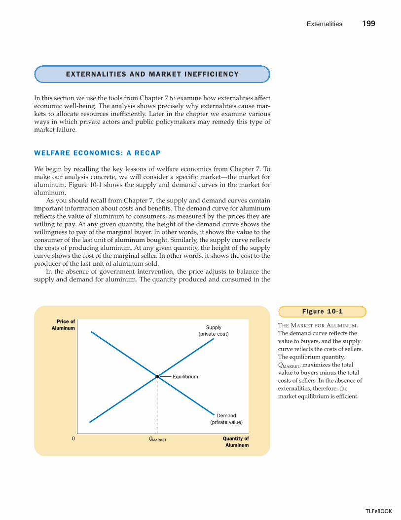
CHAPTER 10 EXTERNALITIES 207
EXTERNALITIES AND MARKET INEFFICIENCY
In this section we use the tools from Chapter 7 to examine how externalities affecteconomic well-being. The analysis shows precisely why externalities cause mar-kets to allocate resources inefficiently. Later in the chapter we examine variousways in which private actors and public policymakers may remedy this type ofmarket failure.
WELFARE ECONOMICS: A RECAP
We begin by recalling the key lessons of welfare economics from Chapter 7. Tomake our analysis concrete, we will consider a specific market—the market foraluminum. Figure 10-1 shows the supply and demand curves in the market foraluminum.
As you should recall from Chapter 7, the supply and demand curves containimportant information about costs and benefits. The demand curve for aluminumreflects the value of aluminum to consumers, as measured by the prices they arewilling to pay. At any given quantity, the height of the demand curve shows thewillingness to pay of the marginal buyer. In other words, it shows the value to theconsumer of the last unit of aluminum bought. Similarly, the supply curve reflectsthe costs of producing aluminum. At any given quantity, the height of the supplycurve shows the cost of the marginal seller. In other words, it shows the cost to theproducer of the last unit of aluminum sold.
In the absence of government intervention, the price adjusts to balance thesupply and demand for aluminum. The quantity produced and consumed in the
Equilibrium
Quantity ofAluminum
0
Price ofAluminum
QMARKET
Demand(private value)
Supply(private cost)
Figure 10-1
THE MARKET FOR ALUMINUM.The demand curve reflects thevalue to buyers, and the supplycurve reflects the costs of sellers.The equilibrium quantity,QMARKET, maximizes the totalvalue to buyers minus the totalcosts of sellers. In the absence ofexternalities, therefore, themarket equilibrium is efficient.
Externalities 199
TLFeBOOK
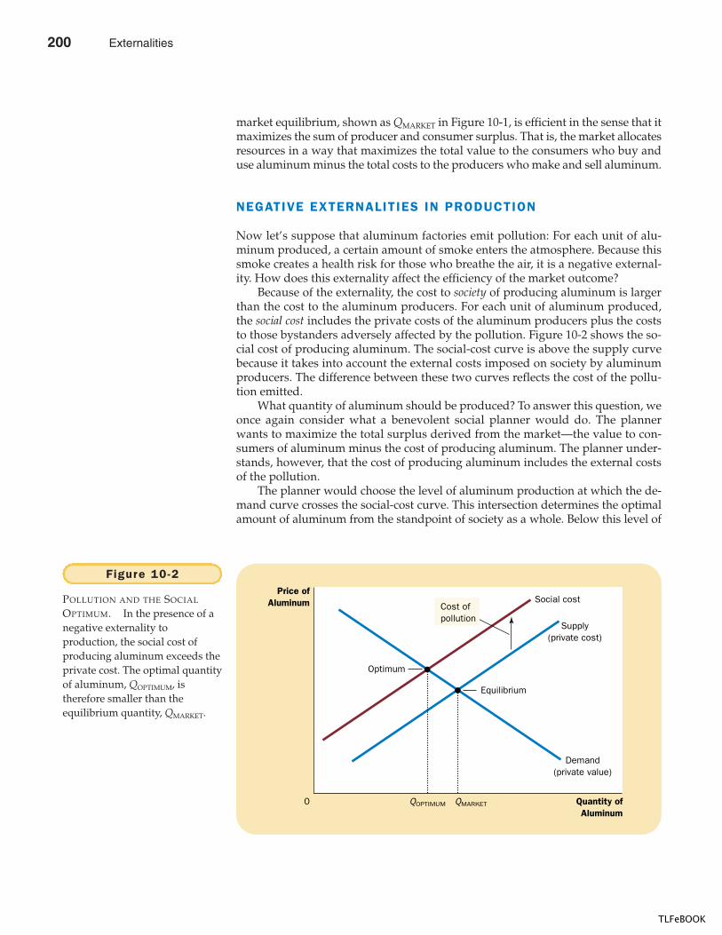
208 PART FOUR THE ECONOMICS OF THE PUBLIC SECTOR
market equilibrium, shown as QMARKET in Figure 10-1, is efficient in the sense that itmaximizes the sum of producer and consumer surplus. That is, the market allocatesresources in a way that maximizes the total value to the consumers who buy anduse aluminum minus the total costs to the producers who make and sell aluminum.
NEGATIVE EXTERNALITIES IN PRODUCTION
Now let’s suppose that aluminum factories emit pollution: For each unit of alu-minum produced, a certain amount of smoke enters the atmosphere. Because thissmoke creates a health risk for those who breathe the air, it is a negative external-ity. How does this externality affect the efficiency of the market outcome?
Because of the externality, the cost to society of producing aluminum is largerthan the cost to the aluminum producers. For each unit of aluminum produced,the social cost includes the private costs of the aluminum producers plus the coststo those bystanders adversely affected by the pollution. Figure 10-2 shows the so-cial cost of producing aluminum. The social-cost curve is above the supply curvebecause it takes into account the external costs imposed on society by aluminumproducers. The difference between these two curves reflects the cost of the pollu-tion emitted.
What quantity of aluminum should be produced? To answer this question, weonce again consider what a benevolent social planner would do. The plannerwants to maximize the total surplus derived from the market—the value to con-sumers of aluminum minus the cost of producing aluminum. The planner under-stands, however, that the cost of producing aluminum includes the external costsof the pollution.
The planner would choose the level of aluminum production at which the de-mand curve crosses the social-cost curve. This intersection determines the optimalamount of aluminum from the standpoint of society as a whole. Below this level of
Equilibrium
Quantity ofAluminum
0
Price ofAluminum
QMARKET
Demand(private value)
Supply(private cost)
Social cost
QOPTIMUM
Optimum
Cost ofpollution
Figure 10-2
POLLUTION AND THE SOCIAL
OPTIMUM. In the presence of anegative externality toproduction, the social cost ofproducing aluminum exceeds theprivate cost. The optimal quantityof aluminum, QOPTIMUM, istherefore smaller than theequilibrium quantity, QMARKET.
200 Externalities
TLFeBOOK
CHAPTER 10 EXTERNALITIES 209
production, the value of the aluminum to consumers (as measured by the height ofthe demand curve) exceeds the social cost of producing it (as measured by the heightof the social-cost curve). The planner does not produce more than this level becausethe social cost of producing additional aluminum exceeds the value to consumers.
Note that the equilibrium quantity of aluminum, QMARKET, is larger than thesocially optimal quantity, QOPTIMUM. The reason for this inefficiency is that the mar-ket equilibrium reflects only the private costs of production. In the market equilib-rium, the marginal consumer values aluminum at less than the social cost ofproducing it. That is, at QMARKET the demand curve lies below the social-cost curve.Thus, reducing aluminum production and consumption below the market equi-librium level raises total economic well-being.
How can the social planner achieve the optimal outcome? One way would beto tax aluminum producers for each ton of aluminum sold. The tax would shift thesupply curve for aluminum upward by the size of the tax. If the tax accurately re-flected the social cost of smoke released into the atmosphere, the new supply curvewould coincide with the social-cost curve. In the new market equilibrium, alu-minum producers would produce the socially optimal quantity of aluminum.
The use of such a tax is called internalizing the externality because it givesbuyers and sellers in the market an incentive to take account of the external effectsof their actions. Aluminum producers would, in essence, take the costs of pollutioninto account when deciding how much aluminum to supply because the tax nowmakes them pay for these external costs. Later in this chapter we consider otherways in which policymakers can deal with externalities.
POSITIVE EXTERNALITIES IN PRODUCTION
Although in some markets the social cost of production exceeds the private cost, inother markets the opposite is the case. In these markets, the externality benefitsbystanders, so the social cost of production is less than the private cost. One ex-ample is the market for industrial robots.
“All I can say is that if being a leading manufacturer means being a leading polluter, so be it.”
internal iz ing an external ityaltering incentives so that peopletake account of the external effects oftheir actions
Externalities 201
TLFeBOOK
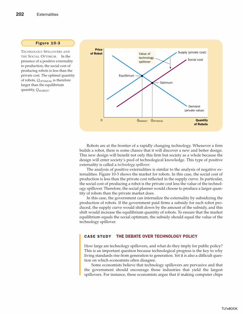
210 PART FOUR THE ECONOMICS OF THE PUBLIC SECTOR
CASE STUDY THE DEBATE OVER TECHNOLOGY POLICY
How large are technology spillovers, and what do they imply for public policy?This is an important question because technological progress is the key to whyliving standards rise from generation to generation. Yet it is also a difficult ques-tion on which economists often disagree.
Some economists believe that technology spillovers are pervasive and thatthe government should encourage those industries that yield the largestspillovers. For instance, these economists argue that if making computer chips
Robots are at the frontier of a rapidly changing technology. Whenever a firmbuilds a robot, there is some chance that it will discover a new and better design.This new design will benefit not only this firm but society as a whole because thedesign will enter society’s pool of technological knowledge. This type of positiveexternality is called a technology spillover.
The analysis of positive externalities is similar to the analysis of negative ex-ternalities. Figure 10-3 shows the market for robots. In this case, the social cost ofproduction is less than the private cost reflected in the supply curve. In particular,the social cost of producing a robot is the private cost less the value of the technol-ogy spillover. Therefore, the social planner would choose to produce a larger quan-tity of robots than the private market does.
In this case, the government can internalize the externality by subsidizing theproduction of robots. If the government paid firms a subsidy for each robot pro-duced, the supply curve would shift down by the amount of the subsidy, and thisshift would increase the equilibrium quantity of robots. To ensure that the marketequilibrium equals the social optimum, the subsidy should equal the value of thetechnology spillover.
Quantityof Robots
0
Priceof Robot
QOPTIMUM
Demand(private value)
Supply (private cost)
Social cost
QMARKET
Value oftechnologyspillover
Equilibrium
Optimum
Figure 10-3
TECHNOLOGY SPILLOVERS AND
THE SOCIAL OPTIMUM. In thepresence of a positive externalityto production, the social cost ofproducing robots is less than theprivate cost. The optimal quantityof robots, QOPTIMUM, is thereforelarger than the equilibriumquantity, QMARKET.
202 Externalities
TLFeBOOK
CHAPTER 10 EXTERNALITIES 211
yields greater spillovers than making potato chips, then the government shoulduse the tax laws to encourage the production of computer chips relative to theproduction of potato chips. Government intervention in the economy that aimsto promote technology-enhancing industries is called technology policy.
Other economists are skeptical about technology policy. Even if technologyspillovers are common, the success of a technology policy requires that thegovernment be able to measure the size of the spillovers from different mar-kets. This measurement problem is difficult at best. Moreover, without precisemeasurements, the political system may end up subsidizing those industrieswith the most political clout, rather than those that yield the largest positiveexternalities.
One type of technology policy that most economists endorse is patent pro-tection. The patent laws protect the rights of inventors by giving them exclusiveuse of their inventions for a period of time. When a firm makes a technologicalbreakthrough, it can patent the idea and capture much of the economic benefitfor itself. The patent is said to internalize the externality by giving the firm aproperty right over its invention. If other firms want to use the new technology,they would have to obtain permission from the inventing firm and pay it someroyalty. Thus, the patent system gives firms a greater incentive to engage in re-search and other activities that advance technology.
EXTERNALITIES IN CONSUMPTION
The externalities we have discussed so far are associated with the production ofgoods. Some externalities, however, are associated with consumption. The con-sumption of alcohol, for instance, yields negative externalities if consumers aremore likely to drive under its influence and risk the lives of others. Similarly, theconsumption of education yields positive externalities because a more educatedpopulation leads to better government, which benefits everyone.
The analysis of consumption externalities is similar to the analysis of produc-tion externalities. As Figure 10-4 shows, the demand curve does not reflect thevalue to society of the good. Panel (a) shows the case of a negative consumptionexternality, such as that associated with alcohol. In this case, the social value is lessthan the private value, and the socially optimal quantity is smaller than the quan-tity determined by the private market. Panel (b) shows the case of a positive con-sumption externality, like that of education. In this case, the social value is greaterthan the private value, and the socially optimal quantity is greater than the quan-tity determined by the private market.
Once again, the government can correct the market failure by inducing marketparticipants to internalize the externality. The appropriate response in the case ofconsumption externalities is similar to that in the case of production externalities.To move the market equilibrium closer to the social optimum, a negative external-ity requires a tax, and a positive externality requires a subsidy. In fact, that is ex-actly the policy the government follows: Alcoholic beverages are among the mosthighly taxed goods in our economy, and education is heavily subsidized throughpublic schools and government scholarships.
As you may have noticed, these examples of externalities lead to some gen-eral lessons: Negative externalities in production or consumption lead markets to pro-duce a larger quantity than is socially desirable. Positive externalities in production
Externalities 203
TLFeBOOK
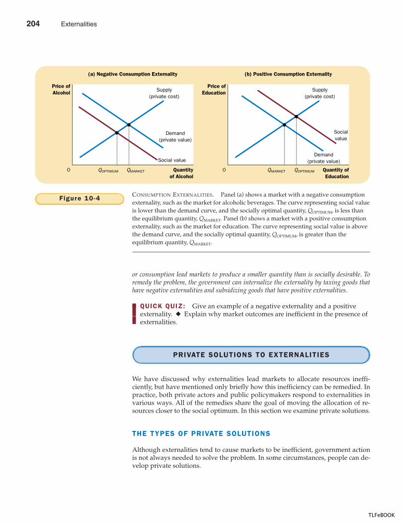
212 PART FOUR THE ECONOMICS OF THE PUBLIC SECTOR
or consumption lead markets to produce a smaller quantity than is socially desirable. Toremedy the problem, the government can internalize the externality by taxing goods thathave negative externalities and subsidizing goods that have positive externalities.
QUICK QUIZ: Give an example of a negative externality and a positive externality. � Explain why market outcomes are inefficient in the presence of externalities.
PRIVATE SOLUTIONS TO EXTERNALITIES
We have discussed why externalities lead markets to allocate resources ineffi-ciently, but have mentioned only briefly how this inefficiency can be remedied. Inpractice, both private actors and public policymakers respond to externalities invarious ways. All of the remedies share the goal of moving the allocation of re-sources closer to the social optimum. In this section we examine private solutions.
THE TYPES OF PRIVATE SOLUTIONS
Although externalities tend to cause markets to be inefficient, government actionis not always needed to solve the problem. In some circumstances, people can de-velop private solutions.
Quantityof Alcohol
0
Price ofAlcohol
QMARKET
Demand(private value)
Supply(private cost)
Social value
QOPTIMUM
(a) Negative Consumption Externality
Quantity ofEducation
0
Price ofEducation
QMARKET
Demand(private value)
Socialvalue
QOPTIMUM
(b) Positive Consumption Externality
Supply(private cost)
Figure 10-4 CONSUMPTION EXTERNALITIES. Panel (a) shows a market with a negative consumptionexternality, such as the market for alcoholic beverages. The curve representing social valueis lower than the demand curve, and the socially optimal quantity, QOPTIMUM, is less thanthe equilibrium quantity, QMARKET. Panel (b) shows a market with a positive consumptionexternality, such as the market for education. The curve representing social value is abovethe demand curve, and the socially optimal quantity, QOPTIMUM, is greater than theequilibrium quantity, QMARKET.
204 Externalities
TLFeBOOK
CHAPTER 10 EXTERNALITIES 213
Sometimes, the problem of externalities is solved with moral codes and socialsanctions. Consider, for instance, why most people do not litter. Although there arelaws against littering, these laws are not vigorously enforced. Most people do notlitter just because it is the wrong thing to do. The Golden Rule taught to most chil-dren says, “Do unto others as you would have them do unto you.” This moral in-junction tells us to take account of how our actions affect other people. Ineconomic terms, it tells us to internalize externalities.
Another private solution to externalities is charities, many of which are estab-lished to deal with externalities. For example, the Sierra Club, whose goal is to pro-tect the environment, is a nonprofit organization funded with private donations. Asanother example, colleges and universities receive gifts from alumni, corporations,and foundations in part because education has positive externalities for society.
The private market can often solve the problem of externalities by relying onthe self-interest of the relevant parties. Sometimes the solution takes the form of in-tegrating different types of business. For example, consider an apple grower and abeekeeper that are located next to each other. Each business confers a positive ex-ternality on the other: By pollinating the flowers on the trees, the bees help the or-chard produce apples. At the same time, the bees use the nectar they get from theapple trees to produce honey. Nonetheless, when the apple grower is decidinghow many trees to plant and the beekeeper is deciding how many bees to keep,they neglect the positive externality. As a result, the apple grower plants too fewtrees and the beekeeper keeps too few bees. These externalities could be internal-ized if the beekeeper bought the apple orchard or if the apple grower bought thebeehive: Both activities would then take place within the same firm, and this sin-gle firm could choose the optimal number of trees and bees. Internalizing exter-nalities is one reason that some firms are involved in different types of business.
Another way for the private market to deal with external effects is for the in-terested parties to enter into a contract. In the foregoing example, a contract be-tween the apple grower and the beekeeper can solve the problem of too few treesand too few bees. The contract can specify the number of trees, the number of bees,and perhaps a payment from one party to the other. By setting the right number oftrees and bees, the contract can solve the inefficiency that normally arises fromthese externalities and make both parties better off.
THE COASE THEOREM
How effective is the private market in dealing with externalities? A famous re-sult, called the Coase theorem after economist Ronald Coase, suggests that it canbe very effective in some circumstances. According to the Coase theorem, if pri-vate parties can bargain without cost over the allocation of resources, then the pri-vate market will always solve the problem of externalities and allocate resourcesefficiently.
To see how the Coase theorem works, consider an example. Suppose that Dickowns a dog named Spot. Spot barks and disturbs Jane, Dick’s neighbor. Dick getsa benefit from owning the dog, but the dog confers a negative externality on Jane.Should Dick be forced to send Spot to the pound, or should Jane have to suffersleepless nights because of Spot’s barking?
Consider first what outcome is socially efficient. A social planner, consideringthe two alternatives, would compare the benefit that Dick gets from the dog to thecost that Jane bears from the barking. If the benefit exceeds the cost, it is efficient
Coase theoremthe proposition that if privateparties can bargain without cost overthe allocation of resources, they cansolve the problem of externalities ontheir own
Externalities 205
TLFeBOOK
214 PART FOUR THE ECONOMICS OF THE PUBLIC SECTOR
for Dick to keep the dog and for Jane to live with the barking. Yet if the cost ex-ceeds the benefit, then Dick should get rid of the dog.
According to the Coase theorem, the private market will reach the efficientoutcome on its own. How? Jane can simply offer to pay Dick to get rid of the dog.Dick will accept the deal if the amount of money Jane offers is greater than the ben-efit of keeping the dog.
By bargaining over the price, Dick and Jane can always reach the efficient out-come. For instance, suppose that Dick gets a $500 benefit from the dog and Janebears an $800 cost from the barking. In this case, Jane can offer Dick $600 to get ridof the dog, and Dick will gladly accept. Both parties are better off than they werebefore, and the efficient outcome is reached.
It is possible, of course, that Jane would not be willing to offer any price thatDick would accept. For instance, suppose that Dick gets a $1,000 benefit from thedog and Jane bears an $800 cost from the barking. In this case, Dick would turndown any offer below $1,000, while Jane would not offer any amount above $800.Therefore, Dick ends up keeping the dog. Given these costs and benefits, however,this outcome is efficient.
So far, we have assumed that Dick has the legal right to keep a barking dog. Inother words, we have assumed that Dick can keep Spot unless Jane pays himenough to induce him to give up the dog voluntarily. How different would theoutcome be, on the other hand, if Jane had the legal right to peace and quiet?
According to the Coase theorem, the initial distribution of rights does not mat-ter for the market’s ability to reach the efficient outcome. For instance, supposethat Jane can legally compel Dick to get rid of the dog. Although having this rightworks to Jane’s advantage, it probably will not change the outcome. In this case,Dick can offer to pay Jane to allow him to keep the dog. If the benefit of the dog toDick exceeds the cost of the barking to Jane, then Dick and Jane will strike a bar-gain in which Dick keeps the dog.
Although Dick and Jane can reach the efficient outcome regardless of howrights are initially distributed, the distribution of rights is not irrelevant: It deter-mines the distribution of economic well-being. Whether Dick has the right to abarking dog or Jane the right to peace and quiet determines who pays whom in thefinal bargain. But, in either case, the two parties can bargain with each other andsolve the externality problem. Dick will end up keeping the dog only if the benefitexceeds the cost.
To sum up: The Coase theorem says that private economic actors can solve the prob-lem of externalities among themselves. Whatever the initial distribution of rights, the in-terested parties can always reach a bargain in which everyone is better off and the outcomeis efficient.
WHY PRIVATE SOLUTIONS DO NOT ALWAYS WORK
Despite the appealing logic of the Coase theorem, private actors on their own of-ten fail to resolve the problems caused by externalities. The Coase theorem appliesonly when the interested parties have no trouble reaching and enforcing an agree-ment. In the real world, however, bargaining does not always work, even when amutually beneficial agreement is possible.
Sometimes the interested parties fail to solve an externality problem becauseof transaction costs, the costs that parties incur in the process of agreeing to andfollowing through on a bargain. In our example, imagine that Dick and Jane speak
transaction coststhe costs that parties incur in theprocess of agreeing and followingthrough on a bargain
206 Externalities
TLFeBOOK
CHAPTER 10 EXTERNALITIES 215
different languages so that, to reach an agreement, they will need to hire a transla-tor. If the benefit of solving the barking problem is less than the cost of the transla-tor, Dick and Jane might choose to leave the problem unsolved. In more realisticexamples, the transaction costs are the expenses not of translators but of thelawyers required to draft and enforce contracts.
Other times bargaining simply breaks down. The recurrence of wars and laborstrikes shows that reaching agreement can be difficult and that failing to reachagreement can be costly. The problem is often that each party tries to hold out fora better deal. For example, suppose that Dick gets a $500 benefit from the dog, andJane bears an $800 cost from the barking. Although it is efficient for Jane to payDick to get rid of the dog, there are many prices that could lead to this outcome.Dick might demand $750, and Jane might offer only $550. As they haggle over theprice, the inefficient outcome with the barking dog persists.
Reaching an efficient bargain is especially difficult when the number of inter-ested parties is large because coordinating everyone is costly. For example, con-sider a factory that pollutes the water of a nearby lake. The pollution confers anegative externality on the local fishermen. According to the Coase theorem, if thepollution is inefficient, then the factory and the fishermen could reach a bargain inwhich the fishermen pay the factory not to pollute. If there are many fishermen,however, trying to coordinate them all to bargain with the factory may be almostimpossible.
When private bargaining does not work, the government can sometimes playa role. The government is an institution designed for collective action. In this ex-ample, the government can act on behalf of the fishermen, even when it is imprac-tical for the fishermen to act for themselves. In the next section, we examine howthe government can try to remedy the problem of externalities.
QUICK QUIZ: Give an example of a private solution to an externality.� What is the Coase theorem? � Why are private economic actors sometimes unable to solve the problems caused by an externality?
PUBLIC POLICIES TOWARD EXTERNALITIES
When an externality causes a market to reach an inefficient allocation of resources,the government can respond in one of two ways. Command-and-control policies reg-ulate behavior directly. Market-based policies provide incentives so that private de-cisionmakers will choose to solve the problem on their own.
REGULATION
The government can remedy an externality by making certain behaviors either re-quired or forbidden. For example, it is a crime to dump poisonous chemicals intothe water supply. In this case, the external costs to society far exceed the benefits tothe polluter. The government therefore institutes a command-and-control policythat prohibits this act altogether.
In most cases of pollution, however, the situation is not this simple. Despitethe stated goals of some environmentalists, it would be impossible to prohibit all
Externalities 207
TLFeBOOK
216 PART FOUR THE ECONOMICS OF THE PUBLIC SECTOR
polluting activity. For example, virtually all forms of transportation—even thehorse—produce some undesirable polluting by-products. But it would not be sen-sible for the government to ban all transportation. Thus, instead of trying to erad-icate pollution altogether, society has to weigh the costs and benefits to decide thekinds and quantities of pollution it will allow. In the United States, the Environ-mental Protection Agency (EPA) is the government agency with the task of devel-oping and enforcing regulations aimed at protecting the environment.
Environmental regulations can take many forms. Sometimes the EPA dictatesa maximum level of pollution that a factory may emit. Other times the EPA re-quires that firms adopt a particular technology to reduce emissions. In all cases, todesign good rules, the government regulators need to know the details about spe-cific industries and about the alternative technologies that those industries couldadopt. This information is often difficult for government regulators to obtain.
PIGOVIAN TAXES AND SUBSIDIES
Instead of regulating behavior in response to an externality, the government can usemarket-based policies to align private incentives with social efficiency. For instance,as we saw earlier, the government can internalize the externality by taxing activitiesthat have negative externalities and subsidizing activities that have positive exter-nalities. Taxes enacted to correct the effects of negative externalities are called Pigov-ian taxes, after economist Arthur Pigou (1877–1959), an early advocate of their use.
Economists usually prefer Pigovian taxes over regulations as a way to dealwith pollution because they can reduce pollution at a lower cost to society. To seewhy, let us consider an example.
Suppose that two factories—a paper mill and a steel mill—are each dumping500 tons of glop into a river each year. The EPA decides that it wants to reduce theamount of pollution. It considers two solutions:
� Regulation: The EPA could tell each factory to reduce its pollution to 300 tonsof glop per year.
� Pigovian tax: The EPA could levy a tax on each factory of $50,000 for each tonof glop it emits.
The regulation would dictate a level of pollution, whereas the tax would give fac-tory owners an economic incentive to reduce pollution. Which solution do youthink is better?
Most economists would prefer the tax. They would first point out that a tax isjust as effective as a regulation in reducing the overall level of pollution. The EPAcan achieve whatever level of pollution it wants by setting the tax at the appropri-ate level. The higher the tax, the larger the reduction in pollution. Indeed, if the taxis high enough, the factories will close down altogether, reducing pollution to zero.
The reason why economists would prefer the tax is that it reduces pollutionmore efficiently. The regulation requires each factory to reduce pollution by thesame amount, but an equal reduction is not necessarily the least expensive way toclean up the water. It is possible that the paper mill can reduce pollution at lowercost than the steel mill. If so, the paper mill would respond to the tax by reducingpollution substantially to avoid the tax, whereas the steel mill would respond byreducing pollution less and paying the tax.
Pigovian taxa tax enacted to correct the effects ofa negative externality
208 Externalities
TLFeBOOK
CHAPTER 10 EXTERNALITIES 217
CASE STUDY WHY IS GASOLINE TAXED SO HEAVILY?
In many countries, gasoline is among the most heavily taxed goods in the econ-omy. In the United States, for instance, almost half of what drivers pay for gaso-line goes to the gas tax. In many European countries, the tax is even larger andthe price of gasoline is three or four times the U.S. price.
Why is this tax so common? One answer is that the gas tax is a Pigovian taxaimed at correcting three negative externalities associated with driving:
� Congestion: If you have ever been stuck in bumper-to-bumper traffic, youhave probably wished that there were fewer cars on the road. A gasoline taxkeeps congestion down by encouraging people to take public transporta-tion, car pool more often, and live closer to work.
� Accidents: Whenever a person buys a large car or a sport utility vehicle,he makes himself safer, but he puts his neighbors at risk. According to theNational Highway Traffic Safety Administration, a person driving a typicalcar is five times as likely to die if hit by a sport utility vehicle than ifhit by another car. The gas tax is an indirect way of making peoplepay when their large, gas-guzzling vehicles impose risk on others, which inturn makes them take account of this risk when choosing what vehicle topurchase.
� Pollution: The burning of fossil fuels such as gasoline is widely believed tobe the cause of global warming. Experts disagree about how dangerous thisthreat is, but there is no doubt that the gas tax reduces the risk by reducingthe use of gasoline.
So the gas tax, rather than causing deadweight losses like most taxes, actuallymakes the economy work better. It means less traffic congestion, safer roads,and a cleaner environment.
In essence, the Pigovian tax places a price on the right to pollute. Just as mar-kets allocate goods to those buyers who value them most highly, a Pigovian tax al-locates pollution to those factories that face the highest cost of reducing it.Whatever the level of pollution the EPA chooses, it can achieve this goal at the low-est total cost using a tax.
Economists also argue that Pigovian taxes are better for the environment. Underthe command-and-control policy of regulation, factories have no reason to reduceemission further once they have reached the target of 300 tons of glop. By contrast,the tax gives the factories an incentive to develop cleaner technologies, because acleaner technology would reduce the amount of tax the factory has to pay.
Pigovian taxes are unlike most other taxes. As we discussed in Chapter 8, mosttaxes distort incentives and move the allocation of resources away from the socialoptimum. The reduction in economic well-being—that is, in consumer and pro-ducer surplus—exceeds the amount of revenue the government raises, resulting ina deadweight loss. By contrast, when externalities are present, society also caresabout the well-being of the bystanders who are affected. Pigovian taxes correct in-centives for the presence of externalities and thereby move the allocation of re-sources closer to the social optimum. Thus, while Pigovian taxes raise revenue forthe government, they enhance economic efficiency.
“IF THE GAS TAX WERE ANY LARGER, I’DTAKE THE BUS.”
Externalities 209
TLFeBOOK
218 PART FOUR THE ECONOMICS OF THE PUBLIC SECTOR
TRADABLE POLLUTION PERMITS
Returning to our example of the paper mill and the steel mill, let us suppose that,despite the advice of its economists, the EPA adopts the regulation and requireseach factory to reduce its pollution to 300 tons of glop per year. Then one day, afterthe regulation is in place and both mills have complied, the two firms go to theEPA with a proposal. The steel mill wants to increase its emission of glop by 100tons. The paper mill has agreed to reduce its emission by the same amount ifthe steel mill pays it $5 million. Should the EPA allow the two factories to makethis deal?
From the standpoint of economic efficiency, allowing the deal is good policy.The deal must make the owners of the two factories better off, because they arevoluntarily agreeing to it. Moreover, the deal does not have any external effects be-cause the total amount of pollution remains the same. Thus, social welfare is en-hanced by allowing the paper mill to sell its right to pollute to the steel mill.
The same logic applies to any voluntary transfer of the right to pollute fromone firm to another. If the EPA allows firms to make these deals, it will, in essence,have created a new scarce resource: pollution permits. A market to trade these per-mits will eventually develop, and that market will be governed by the forces ofsupply and demand. The invisible hand will ensure that this new market effi-ciently allocates the right to pollute. The firms that can reduce pollution only athigh cost will be willing to pay the most for the pollution permits. The firms thatcan reduce pollution at low cost will prefer to sell whatever permits they have.
One advantage of allowing a market for pollution permits is that the initial al-location of pollution permits among firms does not matter from the standpoint ofeconomic efficiency. The logic behind this conclusion is similar to that behind theCoase theorem. Those firms that can reduce pollution most easily would be will-ing to sell whatever permits they get, and those firms that can reduce pollutiononly at high cost would be willing to buy whatever permits they need. As long asthere is a free market for the pollution rights, the final allocation will be efficientwhatever the initial allocation.
Although reducing pollution using pollution permits may seem quite differentfrom using Pigovian taxes, in fact the two policies have much in common. In bothcases, firms pay for their pollution. With Pigovian taxes, polluting firms must paya tax to the government. With pollution permits, polluting firms must pay to buythe permit. (Even firms that already own permits must pay to pollute: The oppor-tunity cost of polluting is what they could have received by selling their permitson the open market.) Both Pigovian taxes and pollution permits internalize the ex-ternality of pollution by making it costly for firms to pollute.
The similarity of the two policies can be seen by considering the market forpollution. Both panels in Figure 10-5 show the demand curve for the right to pol-lute. This curve shows that the lower the price of polluting, the more firms willchoose to pollute. In panel (a), the EPA uses a Pigovian tax to set a price for pollu-tion. In this case, the supply curve for pollution rights is perfectly elastic (becausefirms can pollute as much as they want by paying the tax), and the position of thedemand curve determines the quantity of pollution. In panel (b), the EPA sets aquantity of pollution by issuing pollution permits. In this case, the supply curvefor pollution rights is perfectly inelastic (because the quantity of pollution is fixedby the number of permits), and the position of the demand curve determines theprice of pollution. Hence, for any given demand curve for pollution, the EPA can
210 Externalities
TLFeBOOK
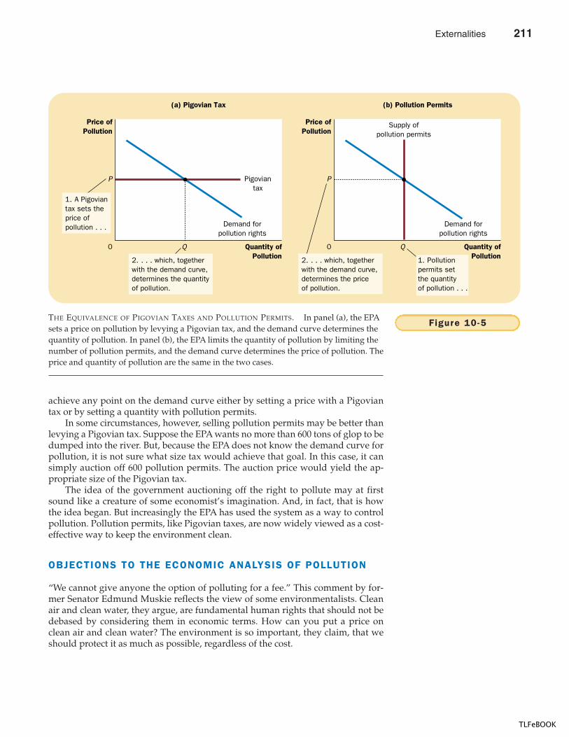
CHAPTER 10 EXTERNALITIES 219
achieve any point on the demand curve either by setting a price with a Pigoviantax or by setting a quantity with pollution permits.
In some circumstances, however, selling pollution permits may be better thanlevying a Pigovian tax. Suppose the EPA wants no more than 600 tons of glop to bedumped into the river. But, because the EPA does not know the demand curve forpollution, it is not sure what size tax would achieve that goal. In this case, it cansimply auction off 600 pollution permits. The auction price would yield the ap-propriate size of the Pigovian tax.
The idea of the government auctioning off the right to pollute may at firstsound like a creature of some economist’s imagination. And, in fact, that is howthe idea began. But increasingly the EPA has used the system as a way to controlpollution. Pollution permits, like Pigovian taxes, are now widely viewed as a cost-effective way to keep the environment clean.
OBJECTIONS TO THE ECONOMIC ANALYSIS OF POLLUTION
“We cannot give anyone the option of polluting for a fee.” This comment by for-mer Senator Edmund Muskie reflects the view of some environmentalists. Cleanair and clean water, they argue, are fundamental human rights that should not bedebased by considering them in economic terms. How can you put a price onclean air and clean water? The environment is so important, they claim, that weshould protect it as much as possible, regardless of the cost.
Quantity ofPollution
0
Price ofPollution
P
Q
Demand forpollution rights
Pigoviantax
(a) Pigovian Tax
Quantity ofPollution
0 Q
Demand forpollution rights
Supply ofpollution permits
(b) Pollution Permits
Price ofPollution
P
2. . . . which, togetherwith the demand curve,determines the quantityof pollution.
2. . . . which, togetherwith the demand curve,determines the priceof pollution.
1. A Pigoviantax sets theprice ofpollution . . .
1. Pollutionpermits setthe quantityof pollution . . .
Figure 10-5THE EQUIVALENCE OF PIGOVIAN TAXES AND POLLUTION PERMITS. In panel (a), the EPAsets a price on pollution by levying a Pigovian tax, and the demand curve determines thequantity of pollution. In panel (b), the EPA limits the quantity of pollution by limiting thenumber of pollution permits, and the demand curve determines the price of pollution. Theprice and quantity of pollution are the same in the two cases.
Externalities 211
TLFeBOOK
220 PART FOUR THE ECONOMICS OF THE PUBLIC SECTOR
Economists have little sympathy with this type of argument. To economists,good environmental policy begins by acknowledging the first of the Ten Principlesof Economics in Chapter 1: People face tradeoffs. Certainly, clean air and clean wa-ter have value. But their value must be compared to their opportunity cost—thatis, to what one must give up to obtain them. Eliminating all pollution is impossi-ble. Trying to eliminate all pollution would reverse many of the technological ad-vances that allow us to enjoy a high standard of living. Few people would bewilling to accept poor nutrition, inadequate medical care, or shoddy housing tomake the environment as clean as possible.
Economists argue that some environmental activists hurt their own cause bynot thinking in economic terms. A clean environment is a good like other goods.Like all normal goods, it has a positive income elasticity: Rich countries can afforda cleaner environment than poor ones and, therefore, usually have more rigorousenvironmental protection. In addition, like most other goods, clean air and waterobey the law of demand: The lower the price of environmental protection, themore the public will want. The economic approach of using pollution permits andPigovian taxes reduces the cost of environmental protection and should, therefore,increase the public’s demand for a clean environment.
QUICK QUIZ: A glue factory and a steel mill emit smoke containing a chemical that is harmful if inhaled in large amounts. Describe three ways the town government might respond to this externality. What are the pros and cons of each of your solutions?
CONCLUSION
The invisible hand is powerful but not omnipotent. A market’s equilibrium maxi-mizes the sum of producer and consumer surplus. When the buyers and sellers inthe market are the only interested parties, this outcome is efficient from the stand-point of society as a whole. But when there are external effects, such as pollution,evaluating a market outcome requires taking into account the well-being of thirdparties as well. In this case, the invisible hand of the marketplace may fail to allo-cate resources efficiently.
In some cases, people can solve the problem of externalities on their own. TheCoase theorem suggests that the interested parties can bargain among themselvesand agree on an efficient solution. Sometimes, however, an efficient outcome can-not be reached, perhaps because the large number of interested parties makes bar-gaining difficult.
When people cannot solve the problem of externalities privately, the govern-ment often steps in. Yet, even now, society should not abandon market forcesentirely. Rather, the government can address the problem by requiring decision-makers to bear the full costs of their actions. Pigovian taxes on emissions and pol-lution permits, for instance, are designed to internalize the externality of pollution.More and more, they are the policy of choice for those interested in protecting theenvironment. Market forces, properly redirected, are often the best remedy for mar-ket failure.
212 Externalities
TLFeBOOK
CHAPTER 10 EXTERNALITIES 221
THIS TONGUE-IN-CHEEK EDITORIAL FROM
THE Economist, an international news-magazine, calls attention to a commonexternality that is not fully appreciated.
M u m ’s t h e W o r d : W h e n C h i l d r e n S h o u l d B eS c r e e n e d a n d N o t H e a r d
We live in increasingly intolerant times.Signs proliferate demanding no smoking,no spitting, no parking, even no walking.. . . Posh clubs and restaurants havelong had “no jeans” rules, but thesedays you can be too smart. Some Lon-don hostelries have “no suits” policies,for fear that boisterous city traders insuits might spoil the atmosphere. Envi-ronmentalists have long demanded allsorts of bans on cars. Mobile telephonesare the latest target: some trains, airlinelounges, restaurants, and even golfcourses are being designated “nophone” areas.
If intolerance really has to be thespirit of this age, The Economist wouldlike to suggest restrictions on anothersource of noise pollution: children. Lestyou dismiss this as mere prejudice, wecan even produce a good economicargument for it. Smoking, driving, and mo-bile phones all cause what economistscall “negative externalities.” That is, thecosts of these activities to other peopletend to exceed the costs to the individuals
of their proclivities. The invisible hand ofthe market fumbles, leading resourcesastray. Thus, because a driver’s privatemotoring costs do not reflect the costs heimposes on others in the form of pollutionand congestion, he uses the car morethan is socially desirable. Likewise, it is ar-gued, smokers take too little care to en-sure that their acrid fumes do not damageother people around them.
Governments typically respond tosuch market failures in two ways. One ishigher taxes, to make polluters pay thefull cost of their anti-social behavior. Theother is regulation, such as emissionstandards or bans on smoking in publicplaces. Both approaches might work forchildren.
For children, just like cigarettes ormobile phones, clearly impose a nega-tive externality on people who are nearthem. Anybody who has suffered a 12-hour flight with a bawling baby in the rowimmediately ahead, or a bored youngsterviciously kicking their seat from behind,will grasp this as quickly as they wouldlove to grasp the youngster’s neck. Hereis a clear case of market failure: parents
do not bear the full costs (indeed youngbabies travel free), so they are too readyto take their noisy brats with them.Where is the invisible hand when it isneeded to administer a good smack?
The solution is obvious. All airlines,trains, and restaurants should createchild-free zones. Put all those children atthe back of the plane and parents mightmake more effort to minimize their noisepollution. And instead of letting childrenpay less and babies go free, they shouldbe charged (or taxed) more than adults,with the revenues used to subsidize seatsimmediately in front of the war-zone.
Passengers could then request ano-children seat, just as they now ask fora no-smoking one. As more womenchoose not to have children and thenumber of older people without youngchildren increases, the demand for child-free travel will expand. Well, yes, it is abit intolerant—but why shouldn’t parentsbe treated as badly as smokers? And atleast there is an obvious airline to pio-neer the scheme: Virgin.
SOURCE: The Economist, December 5, 1998, p. 20.
IN THE NEWS
Children as Externalities
A NEGATIVE EXTERNALITY
Externalities 213
TLFeBOOK
222 PART FOUR THE ECONOMICS OF THE PUBLIC SECTOR
� When a transaction between a buyer and seller directlyaffects a third party, the effect is called an externality.Negative externalities, such as pollution, cause thesocially optimal quantity in a market to be less than theequilibrium quantity. Positive externalities, such astechnology spillovers, cause the socially optimalquantity to be greater than the equilibrium quantity.
� Those affected by externalities can sometimes solve theproblem privately. For instance, when one businessconfers an externality on another business, the twobusinesses can internalize the externality by merging.Alternatively, the interested parties can solve theproblem by negotiating a contract. According to theCoase theorem, if people can bargain without cost, then
they can always reach an agreement in which resourcesare allocated efficiently. In many cases, however,reaching a bargain among the many interested parties isdifficult, so the Coase theorem does not apply.
� When private parties cannot adequately deal withexternal effects, such as pollution, the government oftensteps in. Sometimes the government prevents sociallyinefficient activity by regulating behavior. Other times itinternalizes an externality using Pigovian taxes. Anotherway to protect the environment is for the government toissue a limited number of pollution permits. The endresult of this policy is largely the same as imposingPigovian taxes on polluters.
Summary
externality, p. 206internalizing an externality, p. 209
Coase theorem, p. 213transaction costs, p. 214
Pigovian tax, p. 216
Key Concepts
1. Give an example of a negative externality and anexample of a positive externality.
2. Use a supply-and-demand diagram to explain the effectof a negative externality in production.
3. In what way does the patent system help society solvean externality problem?
4. List some of the ways that the problems caused byexternalities can be solved without governmentintervention.
5. Imagine that you are a nonsmoker sharing a room witha smoker. According to the Coase theorem, whatdetermines whether your roommate smokes in theroom? Is this outcome efficient? How do you and yourroommate reach this solution?
6. What are Pigovian taxes? Why do economists preferthem over regulations as a way to protect theenvironment from pollution?
Questions for Review
1. Do you agree with the following statements? Why orwhy not?a. “The benefits of Pigovian taxes as a way to reduce
pollution have to be weighed against thedeadweight losses that these taxes cause.”
b. “A negative production externality calls for aPigovian tax on producers, whereas a negative
consumption externality calls for a Pigovian tax onconsumers.”
2. Consider the market for fire extinguishers.a. Why might fire extinguishers exhibit positive
externalities in consumption?b. Draw a graph of the market for fire extinguishers,
labeling the demand curve, the social-value
Problems and Appl ications
214 Externalities
TLFeBOOK
CHAPTER 10 EXTERNALITIES 223
curve, the supply curve, and the social-cost curve.
c. Indicate the market equilibrium level of output andthe efficient level of output. Give an intuitiveexplanation for why these quantities differ.
d. If the external benefit is $10 per extinguisher,describe a government policy that would result inthe efficient outcome.
3. Contributions to charitable organizations are deductibleunder the federal income tax. In what way does thisgovernment policy encourage private solutions toexternalities?
4. Ringo loves playing rock and roll music at high volume.Luciano loves opera and hates rock and roll.Unfortunately, they are next-door neighbors in anapartment building with paper-thin walls.a. What is the externality here?b. What command-and-control policy might the
landlord impose? Could such a policy lead to aninefficient outcome?
c. Suppose the landlord lets the tenants do whateverthey want. According to the Coase theorem, howmight Ringo and Luciano reach an efficientoutcome on their own? What might prevent themfrom reaching an efficient outcome?
5. It is rumored that the Swiss government subsidizescattle farming, and that the subsidy is larger in areaswith more tourist attractions. Can you think of a reasonwhy this policy might be efficient?
6. Greater consumption of alcohol leads to more motorvehicle accidents and, thus, imposes costs on peoplewho do not drink and drive.a. Illustrate the market for alcohol, labeling the
demand curve, the social-value curve, the supplycurve, the social-cost curve, the market equilibriumlevel of output, and the efficient level of output.
b. On your graph, shade the area corresponding to thedeadweight loss of the market equilibrium. (Hint:The deadweight loss occurs because some units ofalcohol are consumed for which the social costexceeds the social value.) Explain.
7. Many observers believe that the levels of pollution inour economy are too high.a. If society wishes to reduce overall pollution by a
certain amount, why is it efficient to have differentamounts of reduction at different firms?
b. Command-and-control approaches often rely onuniform reductions among firms. Why are these
approaches generally unable to target the firms thatshould undertake bigger reductions?
c. Economists argue that appropriate Pigovian taxesor tradable pollution rights will result in efficientpollution reduction. How do these approachestarget the firms that should undertake biggerreductions?
8. The Pristine River has two polluting firms on its banks.Acme Industrial and Creative Chemicals each dump 100tons of glop into the river each year. The cost ofreducing glop emissions per ton equals $10 for Acmeand $100 for Creative. The local government wants toreduce overall pollution from 200 tons to 50 tons.a. If the government knew the cost of reduction for
each firm, what reductions would it impose toreach its overall goal? What would be the cost toeach firm and the total cost to the firms together?
b. In a more typical situation, the government wouldnot know the cost of pollution reduction at eachfirm. If the government decided to reach its overallgoal by imposing uniform reductions on the firms,calculate the reduction made by each firm, the costto each firm, and the total cost to the firms together.
c. Compare the total cost of pollution reduction inparts (a) and (b). If the government does not knowthe cost of reduction for each firm, is there stillsome way for it to reduce pollution to 50 tons at thetotal cost you calculated in part (a)? Explain.
9. Figure 10-5 shows that for any given demand curve forthe right to pollute, the government can achieve thesame outcome either by setting a price with a Pigoviantax or by setting a quantity with pollution permits.Suppose there is a sharp improvement in the technologyfor controlling pollution.a. Using graphs similar to those in Figure 10-5,
illustrate the effect of this development on thedemand for pollution rights.
b. What is the effect on the price and quantity ofpollution under each regulatory system? Explain.
10. Suppose that the government decides to issue tradablepermits for a certain form of pollution.a. Does it matter for economic efficiency whether the
government distributes or auctions the permits?Does it matter in any other ways?
b. If the government chooses to distribute the permits,does the allocation of permits among firms matterfor efficiency? Does it matter in any other ways?
11. The primary cause of global warming is carbon dioxide,which enters the atmosphere in varying amounts from
Externalities 215
TLFeBOOK
224 PART FOUR THE ECONOMICS OF THE PUBLIC SECTOR
different countries but is distributed equally around theglobe within a year. In an article in The Boston Globe (July3, 1990), Martin and Kathleen Feldstein argue that thecorrect approach to global warming is “not to askindividual countries to stabilize their emissions ofcarbon dioxide at current levels,” as some havesuggested. Instead, they argue that “carbon dioxideemissions should be reduced in countries where thecosts are least, and the countries that bear that burdenshould be compensated by the rest of the world.”a. Why is international cooperation necessary to reach
an efficient outcome?b. Is it possible to devise a compensation scheme such
that all countries would be better off than under asystem of uniform emission reductions? Explain.
12. Some people object to market-based policies to reducepollution, claiming that they place a dollar value oncleaning our air and water. Economists reply thatsociety implicitly places a dollar value on environmentalcleanup even under command-and-control policies.Discuss why this is true.
13. (This problem is challenging.) There are three industrialfirms in Happy Valley.
INITIAL COST OF REDUCING
FIRM POLLUTION LEVEL POLLUTION BY 1 UNIT
A 70 units $20B 80 25C 50 10
The government wants to reduce pollution to 120 units,so it gives each firm 40 tradable pollution permits.a. Who sells permits and how many do they sell?
Who buys permits and how many do they buy?Briefly explain why the sellers and buyers are eachwilling to do so. What is the total cost of pollutionreduction in this situation?
b. How much higher would the costs of pollutionreduction be if the permits could not be traded?
216 Externalities
TLFeBOOK
IN THIS CHAPTERYOU WILL . . .
Examine why peop letend to use commonresources too much
Cons ider some o fthe impor tant
common resourcesin our economy
Cons ider some o fthe impor tant
pub l ic goods in oureconomy
Learn the def in ingcharacter ist ics o fpub l ic goods and
common resources
Examine whypr ivate marketsfa i l to p rov idepub l ic goods
See why the cost -benef i t ana lys is
o f pub l ic goods isboth necessar y
and d i f f icu l t
An old song lyric maintains that “the best things in life are free.” A moment’sthought reveals a long list of goods that the songwriter could have had in mind. Na-ture provides some of them, such as rivers, mountains, beaches, lakes, and oceans.The government provides others, such as playgrounds, parks, and parades. In eachcase, people do not pay a fee when they choose to enjoy the benefit of the good.
Free goods provide a special challenge for economic analysis. Most goods inour economy are allocated in markets, where buyers pay for what they receive andsellers are paid for what they provide. For these goods, prices are the signals thatguide the decisions of buyers and sellers. When goods are available free of charge,however, the market forces that normally allocate resources in our economy areabsent.
In this chapter we examine the problems that arise for goods without marketprices. Our analysis will shed light on one of the Ten Principles of Economics
P U B L I C G O O D S A N D
C O M M O N R E S O U R C E S
225
217
11
TLFeBOOK
226 PART FOUR THE ECONOMICS OF THE PUBLIC SECTOR
in Chapter 1: Governments can sometimes improve market outcomes. When agood does not have a price attached to it, private markets cannot ensure that thegood is produced and consumed in the proper amounts. In such cases, governmentpolicy can potentially remedy the market failure and raise economic well-being.
THE DIFFERENT KINDS OF GOODS
How well do markets work in providing the goods that people want? The answerto this question depends on the good being considered. As we discussed in Chapter7, we can rely on the market to provide the efficient number of ice-cream cones: Theprice of ice-cream cones adjusts to balance supply and demand, and this equilib-rium maximizes the sum of producer and consumer surplus. Yet, as we discussed inChapter 10, we cannot rely on the market to prevent aluminum manufacturers frompolluting the air we breathe: Buyers and sellers in a market typically do not take ac-count of the external effects of their decisions. Thus, markets work well when thegood is ice cream, but they work badly when the good is clean air.
In thinking about the various goods in the economy, it is useful to group themaccording to two characteristics:
� Is the good excludable? Can people be prevented from using the good?� Is the good rival? Does one person’s use of the good diminish another
person’s enjoyment of it?
Using these two characteristics, Figure 11-1 divides goods into four categories:
1. Private goods are both excludable and rival. Consider an ice-cream cone, forexample. An ice-cream cone is excludable because it is possible to preventsomeone from eating an ice-cream cone—you just don’t give it to him. Anice-cream cone is rival because if one person eats an ice-cream cone, anotherperson cannot eat the same cone. Most goods in the economy are privategoods like ice-cream cones. When we analyzed supply and demand inChapters 4, 5, and 6 and the efficiency of markets in Chapters 7, 8, and 9, weimplicitly assumed that goods were both excludable and rival.
2. Public goods are neither excludable nor rival. That is, people cannot beprevented from using a public good, and one person’s enjoyment of a publicgood does not reduce another person’s enjoyment of it. For example, nationaldefense is a public good. Once the country is defended from foreignaggressors, it is impossible to prevent any single person from enjoying thebenefit of this defense. Moreover, when one person enjoys the benefit ofnational defense, he does not reduce the benefit to anyone else.
3. Common resources are rival but not excludable. For example, fish in theocean are a rival good: When one person catches fish, there are fewer fish forthe next person to catch. Yet these fish are not an excludable good because itis difficult to charge fishermen for the fish that they catch.
4. When a good is excludable but not rival, it is an example of a naturalmonopoly. For instance, consider fire protection in a small town. It is easy to
excludab i l i tythe property of a good whereby aperson can be prevented fromusing it
r i va l r ythe property of a good whereby oneperson’s use diminishes otherpeople’s use
pr ivate goodsgoods that are both excludableand rival
publ ic goodsgoods that are neither excludablenor rival
common resourcesgoods that are rival but notexcludable
218 Public Goods and Common Resources
TLFeBOOK
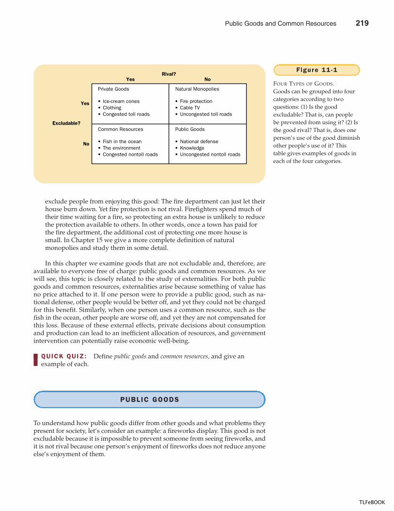
CHAPTER 11 PUBLIC GOODS AND COMMON RESOURCES 227
exclude people from enjoying this good: The fire department can just let theirhouse burn down. Yet fire protection is not rival. Firefighters spend much oftheir time waiting for a fire, so protecting an extra house is unlikely to reducethe protection available to others. In other words, once a town has paid forthe fire department, the additional cost of protecting one more house issmall. In Chapter 15 we give a more complete definition of naturalmonopolies and study them in some detail.
In this chapter we examine goods that are not excludable and, therefore, areavailable to everyone free of charge: public goods and common resources. As wewill see, this topic is closely related to the study of externalities. For both publicgoods and common resources, externalities arise because something of value hasno price attached to it. If one person were to provide a public good, such as na-tional defense, other people would be better off, and yet they could not be chargedfor this benefit. Similarly, when one person uses a common resource, such as thefish in the ocean, other people are worse off, and yet they are not compensated forthis loss. Because of these external effects, private decisions about consumptionand production can lead to an inefficient allocation of resources, and governmentintervention can potentially raise economic well-being.
QUICK QUIZ: Define public goods and common resources, and give an example of each.
PUBLIC GOODS
To understand how public goods differ from other goods and what problems theypresent for society, let’s consider an example: a fireworks display. This good is notexcludable because it is impossible to prevent someone from seeing fireworks, andit is not rival because one person’s enjoyment of fireworks does not reduce anyoneelse’s enjoyment of them.
Rival?
Yes
Yes
• Ice-cream cones• Clothing• Congested toll roads
• Fire protection• Cable TV• Uncongested toll roads
No
Private Goods Natural Monopolies
No
Excludable?
• Fish in the ocean• The environment• Congested nontoll roads
• National defense• Knowledge• Uncongested nontoll roads
Common Resources Public Goods
Figure 11 -1
FOUR TYPES OF GOODS.Goods can be grouped into fourcategories according to twoquestions: (1) Is the goodexcludable? That is, can peoplebe prevented from using it? (2) Isthe good rival? That is, does oneperson’s use of the good diminishother people’s use of it? Thistable gives examples of goods ineach of the four categories.
Public Goods and Common Resources 219
TLFeBOOK
228 PART FOUR THE ECONOMICS OF THE PUBLIC SECTOR
THE FREE-RIDER PROBLEM
The citizens of Smalltown, U.S.A., like seeing fireworks on the Fourth of July. Eachof the town’s 500 residents places a $10 value on the experience. The cost ofputting on a fireworks display is $1,000. Because the $5,000 of benefits exceed the$1,000 of costs, it is efficient for Smalltown residents to see fireworks on the Fourthof July.
Would the private market produce the efficient outcome? Probably not. Imag-ine that Ellen, a Smalltown entrepreneur, decided to put on a fireworks display.Ellen would surely have trouble selling tickets to the event because her potentialcustomers would quickly figure out that they could see the fireworks even withouta ticket. Fireworks are not excludable, so people have an incentive to be free riders.A free rider is a person who receives the benefit of a good but avoids paying for it.
One way to view this market failure is that it arises because of an externality.If Ellen did put on the fireworks display, she would confer an external benefit onthose who saw the display without paying for it. When deciding whether to puton the display, Ellen ignores these external benefits. Even though a fireworks dis-play is socially desirable, it is not privately profitable. As a result, Ellen makes thesocially inefficient decision not to put on the display.
Although the private market fails to supply the fireworks display demandedby Smalltown residents, the solution to Smalltown’s problem is obvious: The localgovernment can sponsor a Fourth of July celebration. The town council can raiseeveryone’s taxes by $2 and use the revenue to hire Ellen to produce the fireworks.Everyone in Smalltown is better off by $8—the $10 in value from the fireworks mi-nus the $2 tax bill. Ellen can help Smalltown reach the efficient outcome as a pub-lic employee even though she could not do so as a private entrepreneur.
The story of Smalltown is simplified, but it is also realistic. In fact, many localgovernments in the United States do pay for fireworks on the Fourth of July. More-over, the story shows a general lesson about public goods: Because public goodsare not excludable, the free-rider problem prevents the private market from sup-plying them. The government, however, can potentially remedy the problem. Ifthe government decides that the total benefits exceed the costs, it can provide thepublic good and pay for it with tax revenue, making everyone better off.
SOME IMPORTANT PUBLIC GOODS
There are many examples of public goods. Here we consider three of the mostimportant.
Nat iona l Defense The defense of the country from foreign aggressors is aclassic example of a public good. It is also one of the most expensive. In 1999 theU.S. federal government spent a total of $277 billion on national defense, or about$1,018 per person. People disagree about whether this amount is too small or toolarge, but almost no one doubts that some government spending for national de-fense is necessary. Even economists who advocate small government agree that thenational defense is a public good the government should provide.
Bas ic Research The creation of knowledge is a public good. If a mathe-matician proves a new theorem, the theorem enters the general pool of knowledge
f r ee r idera person who receives the benefit of agood but avoids paying for it
220 Public Goods and Common Resources
TLFeBOOK
CHAPTER 11 PUBLIC GOODS AND COMMON RESOURCES 229
that anyone can use without charge. Because knowledge is a public good, profit-seeking firms tend to free ride on the knowledge created by others and, as a result,devote too few resources to the creation of knowledge.
In evaluating the appropriate policy toward knowledge creation, it is impor-tant to distinguish general knowledge from specific, technological knowledge.Specific, technological knowledge, such as the invention of a better battery, can bepatented. The inventor thus obtains much of the benefit of his invention, althoughcertainly not all of it. By contrast, a mathematician cannot patent a theorem; suchgeneral knowledge is freely available to everyone. In other words, the patent sys-tem makes specific, technological knowledge excludable, whereas general knowl-edge is not excludable.
The government tries to provide the public good of general knowledge in var-ious ways. Government agencies, such as the National Institutes of Health and theNational Science Foundation, subsidize basic research in medicine, mathematics,physics, chemistry, biology, and even economics. Some people justify governmentfunding of the space program on the grounds that it adds to society’s pool ofknowledge. Certainly, many private goods, including bullet-proof vests and the in-stant drink Tang, use materials that were first developed by scientists and engi-neers trying to land a man on the moon. Determining the appropriate level ofgovernmental support for these endeavors is difficult because the benefits are hardto measure. Moreover, the members of Congress who appropriate funds for re-search usually have little expertise in science and, therefore, are not in the best po-sition to judge what lines of research will produce the largest benefits.
F ight ing Pover ty Many government programs are aimed at helping thepoor. The welfare system (officially called Temporary Assistance for Needy Fami-lies) provides a small income for some poor families. Similarly, the Food Stampprogram subsidizes the purchase of food for those with low incomes, and variousgovernment housing programs make shelter more affordable. These antipovertyprograms are financed by taxes on families that are financially more successful.
“I like the concept if we can do it with no new taxes.”
Public Goods and Common Resources 221
TLFeBOOK
230 PART FOUR THE ECONOMICS OF THE PUBLIC SECTOR
CASE STUDY ARE LIGHTHOUSES PUBLIC GOODS?
Some goods can switch between being public goods and being private goodsdepending on the circumstances. For example, a fireworks display is a publicgood if performed in a town with many residents. Yet if performed at a privateamusement park, such as Walt Disney World, a fireworks display is more like aprivate good because visitors to the park pay for admission.
Another example is a lighthouse. Economists have long used lighthouses asexamples of a public good. Lighthouses are used to mark specific locations sothat passing ships can avoid treacherous waters. The benefit that the lighthouseprovides to the ship captain is neither excludable nor rival, so each captain hasan incentive to free ride by using the lighthouse to navigate without paying forthe service. Because of this free-rider problem, private markets usually fail toprovide the lighthouses that ship captains need. As a result, most lighthousestoday are operated by the government.
Economists disagree among themselves about what role the governmentshould play in fighting poverty. Although we will discuss this debate more fully inChapter 20, here we note one important argument: Advocates of antipoverty pro-grams claim that fighting poverty is a public good.
Suppose that everyone prefers to live in a society without poverty. Even if thispreference is strong and widespread, fighting poverty is not a “good” that the pri-vate market can provide. No single individual can eliminate poverty because theproblem is so large. Moreover, private charity is hard pressed to solve the problem:People who do not donate to charity can free ride on the generosity of others. Inthis case, taxing the wealthy to raise the living standards of the poor can makeeveryone better off. The poor are better off because they now enjoy a higher stan-dard of living, and those paying the taxes are better off because they enjoy livingin a society with less poverty.
USE OF THE LIGHTHOUSE IS FREE TO THE BOAT OWNER. DOES THIS MAKE THE LIGHTHOUSE A PUBLIC GOOD?
222 Public Goods and Common Resources
TLFeBOOK
CHAPTER 11 PUBLIC GOODS AND COMMON RESOURCES 231
In some cases, however, lighthouses may be closer to private goods. On thecoast of England in the nineteenth century, some lighthouses were privatelyowned and operated. The owner of the local lighthouse did not try to chargeship captains for the service but did charge the owner of the nearby port. If theport owner did not pay, the lighthouse owner turned off the light, and shipsavoided that port.
In deciding whether something is a public good, one must determine thenumber of beneficiaries and whether these beneficiaries can be excluded fromenjoying the good. A free-rider problem arises when the number of beneficiariesis large and exclusion of any one of them is impossible. If a lighthouse benefitsmany ship captains, it is a public good. Yet if it primarily benefits a single portowner, it is more like a private good.
THE DIFFICULT JOB OF COST-BENEFIT ANALYSIS
So far we have seen that the government provides public goods because the pri-vate market on its own will not produce an efficient quantity. Yet deciding that thegovernment must play a role is only the first step. The government must then de-termine what kinds of public goods to provide and in what quantities.
Suppose that the government is considering a public project, such as buildinga new highway. To judge whether to build the highway, it must compare the totalbenefits of all those who would use it to the costs of building and maintaining it.To make this decision, the government might hire a team of economists and engi-neers to conduct a study, called a cost-benefit analysis, the goal of which is to es-timate the total costs and benefits of the project to society as a whole.
Cost-benefit analysts have a tough job. Because the highway will be availableto everyone free of charge, there is no price with which to judge the value of thehighway. Simply asking people how much they would value the highway is notreliable. First, quantifying benefits is difficult using the results from a question-naire. Second, respondents have little incentive to tell the truth. Those who woulduse the highway have an incentive to exaggerate the benefit they receive to get thehighway built. Those who would be harmed by the highway have an incentive toexaggerate the costs to them to prevent the highway from being built.
The efficient provision of public goods is, therefore, intrinsically more difficultthan the efficient provision of private goods. Private goods are provided in themarket. Buyers of a private good reveal the value they place on it by the pricesthey are willing to pay. Sellers reveal their costs by the prices they are willing toaccept. By contrast, cost-benefit analysts do not observe any price signals whenevaluating whether the government should provide a public good. Their findingson the costs and benefits of public projects are, therefore, rough approximationsat best.
cost -benef i t ana lys isa study that compares the costs andbenefits to society of providing apublic good
CASE STUDY HOW MUCH IS A LIFE WORTH?
Imagine that you have been elected to serve as a member of your local towncouncil. The town engineer comes to you with a proposal: The town can spend$10,000 to build and operate a traffic light at a town intersection that now hasonly a stop sign. The benefit of the traffic light is increased safety. The engineer
Public Goods and Common Resources 223
TLFeBOOK
232 PART FOUR THE ECONOMICS OF THE PUBLIC SECTOR
estimates, based on data from similar intersections, that the traffic light wouldreduce the risk of a fatal traffic accident over the lifetime of the traffic light from1.6 to 1.1 percent. Should you spend the money for the new light?
To answer this question, you turn to cost-benefit analysis. But you quicklyrun into an obstacle: The costs and benefits must be measured in the same unitsif you are to compare them meaningfully. The cost is measured in dollars, butthe benefit—the possibility of saving a person’s life—is not directly monetary.To make your decision, you have to put a dollar value on a human life.
At first, you may be tempted to conclude that a human life is priceless. Af-ter all, there is probably no amount of money that you could be paid to volun-tarily give up your life or that of a loved one. This suggests that a human lifehas an infinite dollar value.
For the purposes of cost-benefit analysis, however, this answer leads tononsensical results. If we truly placed an infinite value on human life, weshould be placing traffic lights on every street corner. Similarly, we should all bedriving large cars with all the latest safety features, instead of smaller ones withfewer safety features. Yet traffic lights are not at every corner, and people some-times choose to buy small cars without side-impact air bags or antilock brakes.In both our public and private decisions, we are at times willing to risk our livesto save some money.
Once we have accepted the idea that a person’s life does have an implicitdollar value, how can we determine what that value is? One approach, some-times used by courts to award damages in wrongful-death suits, is to look at thetotal amount of money a person would have earned if he or she had lived.Economists are often critical of this approach. It has the bizarre implication thatthe life of a retired or disabled person has no value.
A better way to value human life is to look at the risks that people are vol-untarily willing to take and how much they must be paid for taking them. Mor-tality risk varies across jobs, for example. Construction workers in high-risebuildings face greater risk of death on the job than office workers do. By com-paring wages in risky and less risky occupations, controlling for education, ex-perience, and other determinants of wages, economists can get some senseabout what value people put on their own lives. Studies using this approachconclude that the value of a human life is about $10 million.
EVERYONE WOULD
LIKE TO AVOID THE
RISK OF THIS, BUT AT
WHAT COST?
224 Public Goods and Common Resources
TLFeBOOK
CHAPTER 11 PUBLIC GOODS AND COMMON RESOURCES 233
We can now return to our original example and respond to the town engi-neer. The traffic light reduces the risk of fatality by 0.5 percent. Thus, the ex-pected benefit from having the traffic light is 0.005 � $10 million, or $50,000.This estimate of the benefit well exceeds the cost of $10,000, so you should ap-prove the project.
COST-BENEFIT ANALYSTS OFTEN RUN INTO
hard questions. Here’s an example.
T h e y E x i s t . T h e r e f o r e T h e yA r e . B u t , D o Yo u C a r e ?
BY SAM HOWE VERHOVEK
It sounds like a philosophical cousin tothe age-old question of whether a treefalling in the forest makes a sound if noone is around to hear it. In this case,though, federal officials are seeking toadd an economic variable to the puzzle:Just how much is it worth to you to knowthat a once-dammed river is running wildagain—even if you never visit it?
In the midst of a major study ofwhether or not to breach four huge hy-droelectric dams on the Snake River ineastern Washington, economists withthe Army Corps of Engineers are addinga factor known as “existence value” totheir list of costs and benefits of the con-tentious proposal.
Breaching the dams would restore140 miles of the lower Snake to its wild,free-flowing condition and would, manybiologists argue, stand a good chance ofrevitalizing endangered salmon runs inthe river. Aside from calculating the pro-posal’s effects on jobs, electric bills, andshipping rates, the Government is nowhoping to assign a dollar value to Ameri-cans’ knowledge that a piece of theirwilderness might be regained. . . .
“The idea that you’d be willing topay something for some state of theworld to exist, as you would pay for acommodity or a contract for services, isnot at all crazy,” said Alan Randall, chair-man of the department of agricultural,environmental, and development eco-nomics at Ohio State University. “The
controversy, really, is mostly aboutmeasurability.”
Proponents of the dam-breachingproposal have pointed to polls suggest-ing that Seattle-area residents would bewilling to pay a few extra dollars a monthon their electricity bills into order to savesalmon runs. . . . Economists at theCorps of Engineers have calculated thatbreaching the four Snake River damsand successfully restoring the salmon isan idea for which Americans would bewilling to shell out [in total] as much as$1 billion. . . .
Others question whether such avalue can be accurately measured. “Theonly way to do it is to ask people whatthey would be willing to pay, and in myview you ask people questions like thatand you get very upwardly biased re-sults,” said Jerry Hausman, an econom-ics professor at M.I.T. “When somebodycalls you on the phone to ask, it’s notreal money.”
SOURCE: The New York Times, Week in Review,October 17, 1999, p. 5.
IN THE NEWS
Existence Value
QUICK QUIZ: What is the free-rider problem? � Why does the free-rider problem induce the government to provide public goods? � How should the government decide whether to provide a public good?
COMMON RESOURCES
Common resources, like public goods, are not excludable: They are available free ofcharge to anyone who wants to use them. Common resources are, however, rival:
Public Goods and Common Resources 225
TLFeBOOK
234 PART FOUR THE ECONOMICS OF THE PUBLIC SECTOR
One person’s use of the common resource reduces other people’s enjoyment of it.Thus, common resources give rise to a new problem. Once the good is provided,policymakers need to be concerned about how much it is used. This problem is bestunderstood from the classic parable called the Tragedy of the Commons.
THE TRAGEDY OF THE COMMONS
Consider life in a small medieval town. Of the many economic activities that takeplace in the town, one of the most important is raising sheep. Many of the town’sfamilies own flocks of sheep and support themselves by selling the sheep’s wool,which is used to make clothing.
As our story begins, the sheep spend much of their time grazing on the landsurrounding the town, called the Town Common. No family owns the land. In-stead, the town residents own the land collectively, and all the residents are al-lowed to graze their sheep on it. Collective ownership works well because land isplentiful. As long as everyone can get all the good grazing land they want, theTown Common is not a rival good, and allowing residents’ sheep to graze for freecauses no problems. Everyone in town is happy.
As the years pass, the population of the town grows, and so does the numberof sheep grazing on the Town Common. With a growing number of sheep and afixed amount of land, the land starts to lose its ability to replenish itself. Eventu-ally, the land is grazed so heavily that it becomes barren. With no grass left on theTown Common, raising sheep is impossible, and the town’s once prosperous woolindustry disappears. Many families lose their source of livelihood.
What causes the tragedy? Why do the shepherds allow the sheep populationto grow so large that it destroys the Town Common? The reason is that social andprivate incentives differ. Avoiding the destruction of the grazing land depends onthe collective action of the shepherds. If the shepherds acted together, they couldreduce the sheep population to a size that the Town Common can support. Yet nosingle family has an incentive to reduce the size of its own flock because each flockrepresents only a small part of the problem.
In essence, the Tragedy of the Commons arises because of an externality. Whenone family’s flock grazes on the common land, it reduces the quality of the landavailable for other families. Because people neglect this negative externality whendeciding how many sheep to own, the result is an excessive number of sheep.
If the tragedy had been foreseen, the town could have solved the problemin various ways. It could have regulated the number of sheep in each family’sflock, internalized the externality by taxing sheep, or auctioned off a limited num-ber of sheep-grazing permits. That is, the medieval town could have dealt with theproblem of overgrazing in the way that modern society deals with the problem ofpollution.
In the case of land, however, there is a simpler solution. The town can divideup the land among town families. Each family can enclose its parcel of land with afence and then protect it from excessive grazing. In this way, the land becomes aprivate good rather than a common resource. This outcome in fact occurred dur-ing the enclosure movement in England in the seventeenth century.
The Tragedy of the Commons is a story with a general lesson: When one per-son uses a common resource, he diminishes other people’s enjoyment of it. Be-cause of this negative externality, common resources tend to be used excessively.
Tragedy o f the Commonsa parable that illustrates whycommon resources get used morethan is desirable from the standpointof society as a whole
226 Public Goods and Common Resources
TLFeBOOK
CHAPTER 11 PUBLIC GOODS AND COMMON RESOURCES 235
The government can solve the problem by reducing use of the common resourcethrough regulation or taxes. Alternatively, the government can sometimes turn thecommon resource into a private good.
This lesson has been known for thousands of years. The ancient Greekphilosopher Aristotle pointed out the problem with common resources: “What iscommon to many is taken least care of, for all men have greater regard for what istheir own than for what they possess in common with others.”
SOME IMPORTANT COMMON RESOURCES
There are many examples of common resources. In almost all cases, the same prob-lem arises as in the Tragedy of the Commons: Private decisionmakers use the com-mon resource too much. Governments often regulate behavior or impose fees tomitigate the problem of overuse.
Clean A i r and Water As we discussed in Chapter 10, markets do not ad-equately protect the environment. Pollution is a negative externality that can beremedied with regulations or with Pigovian taxes on polluting activities. One canview this market failure as an example of a common-resource problem. Clean airand clean water are common resources like open grazing land, and excessive pol-lution is like excessive grazing. Environmental degradation is a modern Tragedyof the Commons.
Oi l Poo ls Consider an underground pool of oil so large that it lies undermany properties with different owners. Any of the owners can drill and extract theoil, but when one owner extracts oil, less is available for the others. The oil is acommon resource.
Just as the number of sheep grazing on the Town Common was inefficientlylarge, the number of wells drawing from the oil pool will be inefficiently large. Be-cause each owner who drills a well imposes a negative externality on the otherowners, the benefit to society of drilling a well is less than the benefit to the ownerwho drills it. That is, drilling a well can be privately profitable even when it is so-cially undesirable. If owners of the properties decide individually how many oilwells to drill, they will drill too many.
To ensure that the oil is extracted at lowest cost, some type of joint actionamong the owners is necessary to solve the common-resource problem. The Coasetheorem, which we discussed in Chapter 10, suggests that a private solution mightbe possible. The owners could reach an agreement among themselves about howto extract the oil and divide the profits. In essence, the owners would then act as ifthey were in a single business.
When there are many owners, however, a private solution is more difficult. Inthis case, government regulation could ensure that the oil is extracted efficiently.
Congested Roads Roads can be either public goods or common resources.If a road is not congested, then one person’s use does not affect anyone else. In thiscase, use is not rival, and the road is a public good. Yet if a road is congested, thenuse of that road yields a negative externality. When one person drives on the road,it becomes more crowded, and other people must drive more slowly. In this case,the road is a common resource.
Public Goods and Common Resources 227
TLFeBOOK
236 PART FOUR THE ECONOMICS OF THE PUBLIC SECTOR
One way for the government to address the problem of road congestion is tocharge drivers a toll. A toll is, in essence, a Pigovian tax on the externality of con-gestion. Often, as in the case of local roads, tolls are not a practical solution becausethe cost of collecting them is too high.
Sometimes congestion is a problem only at certain times of day. If a bridge isheavily traveled only during rush hour, for instance, the congestion externality islarger during this time than during other times of day. The efficient way to dealwith these externalities is to charge higher tolls during rush hour. This toll wouldprovide an incentive for drivers to alter their schedules and would reduce trafficwhen congestion is greatest.
Another policy that responds to the problem of road congestion, discussed ina case study in the previous chapter, is the tax on gasoline. Gasoline is a comple-mentary good to driving: An increase in the price of gasoline tends to reduce thequantity of driving demanded. Therefore, a gasoline tax reduces road congestion.
TOLLS ARE A SIMPLE WAY TO SOLVE THE
problem of road congestion and, ac-cording to some economists, are notused as much as they should be. In thisopinion column, economist LesterThurow describes Singapore’s successin dealing with congestion.
E c o n o m i c s o f R o a d P r i c i n g
BY LESTER C. THUROW
Start with a simple observational truth.No city has ever been able to solve itscongestion and pollution problems bybuilding more roads.
Some of the world’s cities have builta lot of roads (Los Angeles) and somehave very few (Shanghai only recently
has had a lot of autos) but the degreesof congestion and pollution don’t differvery much. More roads simply encour-age more people to use their cars, to livefarther away from work, and thus usemore road space. . . . A recent analysisof congestion problems in London cameto the conclusion that London could tear
the entire central city down to makeroom for roads and would still havesomething approaching gridlock.
Economists have always had a the-oretical answer for auto congestion andpollution problems—road pricing. Chargepeople for using roads based on whatroads they use, what time of day and
IN THE NEWS
The Singapore Solution
HOW CAN WE CLEAR THIS MARKET?
228 Public Goods and Common Resources
TLFeBOOK
CHAPTER 11 PUBLIC GOODS AND COMMON RESOURCES 237
A gasoline tax, however, is an imperfect solution to road congestion. The problemis that the gasoline tax affects other decisions besides the amount of driving oncongested roads. For example, the gasoline tax discourages driving on noncon-gested roads, even though there is no congestion externality for these roads.
Fish , Whales , and Other W i ld l i fe Many species of animals are com-mon resources. Fish and whales, for instance, have commercial value, and anyonecan go to the ocean and catch whatever is available. Each person has little incen-tive to maintain the species for the next year. Just as excessive grazing can destroythe Town Common, excessive fishing and whaling can destroy commercially valu-able marine populations.
The ocean remains one of the least regulated common resources. Two prob-lems prevent an easy solution. First, many countries have access to the oceans, soany solution would require international cooperation among countries that hold
year they use those roads, and thedegree to which pollution problems existat the time they are using those roads.Set prices at the levels that yield the op-timal amounts of usage.
Until Singapore decided to try, nocity had ever had the nerve to use roadpricing. Many ideas seem good theo-retically but have some hidden unex-pected flaws. Singapore now has morethan a decade of experience. The sys-tem works! There are no unexpectedflaws. Singapore is the only city on theface of the earth without congestion andauto-induced pollution problems.
In Singapore a series of toll boothssurrounds the central core of the city. Todrive into the city, each car must pay atoll based on the roads being used, thetime of day when the driving will occur,and that day’s pollution problem. Pricesare raised and lowered to get optimalusage.
In addition, Singapore calculates themaximum number of cars that can besupported without pollution outside ofthe central city and auctions off therights to license new cars each month.Different types of plates allow different
degrees of usage. A plate that allowsone to use their car at any time is muchmore expensive than a plate that only al-lows one to use their car on weekends—a time when congestion problems aremuch less intense. Prices depend onsupply and demand.
With this system Singapore endsup not wasting resources on infrastruc-ture projects that won’t cure congestionand pollution problems. The revenue col-lected from the system is used to lowerother taxes.
If that is so, why then did London re-ject road pricing in its recent report on itsauto congestion and pollution problems?They feared that such a system would beseen as too much interference from theheavy hand of government and that thepublic would not put up with a systemthat allows the rich to drive more thanthe poor.
Both arguments ignore the fact thatwe already have toll roads, but new tech-nologies now also make it possible toavoid both problems.
Using bar codes and debit cards, acity can install bar code readers at differ-ent points around the city. As any car
goes by each point a certain amount isdeducted from the driver’s debit card ac-count depending upon weather, time ofday, and location.
Inside the car, the driver has a me-ter that tells him how much he has beencharged and how much remains in hisdebit card account. . . .
If one is an egalitarian and thinksthat driving privileges should be distrib-uted equally (i.e., not based upon in-come) then each auto can be given aspecified debit card balance every yearand those who are willing to drive lesscan sell their unused balances to thosethat want to drive more.
Instead of giving the city extra taxrevenue, this system gives those whoare willing to live near work or to usepublic transit an income supplement.Since poor people drive less than richpeople, the system ends up being anegalitarian redistribution of income fromthe rich to the poor.
SOURCE: The Boston Globe, February 28, 1995, p. 40.
Public Goods and Common Resources 229
TLFeBOOK
238 PART FOUR THE ECONOMICS OF THE PUBLIC SECTOR
CASE STUDY WHY THE COW IS NOT EXTINCT
Throughout history, many species of animals have been threatened with extinc-tion. When Europeans first arrived in North America, more than 60 million
different values. Second, because the oceans are so vast, enforcing any agreementis difficult. As a result, fishing rights have been a frequent source of internationaltension among normally friendly countries.
Within the United States, various laws aim to protect fish and other wildlife.For example, the government charges for fishing and hunting licenses, and it re-stricts the lengths of the fishing and hunting seasons. Fishermen are often re-quired to throw back small fish, and hunters can kill only a limited number ofanimals. All these laws reduce the use of a common resource and help maintainanimal populations.
NATIONAL PARKS, LIKE ROADS, CAN BE
either public goods or common re-sources. If congestion is not a problem,a visit to a park is not rival. Yet once apark becomes popular, it suffers fromthe same problem as the Town Com-mon. In this opinion column, an econo-mist argues for the use of higherentrance fees to solve the problem.
S a v e t h e P a r k s , a n d M a k e a P r o f i t
BY ALLEN R. SANDERSON
It is common knowledge that our nationalparks are overcrowded, deteriorating,and broke. Some suggest that we ad-dress these problems by requiring reser-vations, closing some areas, or asking
Congress to increase financing to theNational Park Service. But to an econo-mist, there is a more obvious solution:Raise the entrance fees.
When the National Park Servicewas established in 1916, the admissionprice to Yellowstone for a family of fivearriving by car was $7.50; today, theprice is only $10. Had the 1916 pricebeen adjusted for inflation, the compara-ble 1995 fee would be $120 a day—about what that family would pay for aday of rides at Disney World, . . . or tosee a professional football game.
No wonder our national parks areoverrun and overtrampled. We are treat-ing our natural and historical treasures asfree goods when they are not. We are ig-noring the costs of maintaining theseplaces and rationing by congestion—when it gets too crowded, no more visi-tors are allowed—perhaps the mostinefficient way to allocate scarce re-sources. The price of a family’s day in anational park has not kept pace withmost other forms of recreation. Sys-temwide, it barely averages a dollar aperson. . . .
An increase in daily user fees to,say, $20 per person would either reduce
the overcrowding and deterioration inour parks by cutting down on the numberof visitors or it would substantially raisefee revenues for the Park Service (as-suming that legislation was passed thatwould let the park system keep thismoney). Greater revenue is the morelikely outcome. After spending severalhundred dollars to reach YellowstonePark, few people would be deterred byanother $20.
The added revenues would bringmore possibilities for outdoor recreation,both through expansion of the NationalPark Service and by encouraging privateentrepreneurs to carve out and operatetheir own parks, something they cannotdo alongside a public competitor givingaway his product well below cost.
It is time to put our money whereour Patagonia outfits are: Either we valuethe Grand Canyon and Yosemite andwon’t complain about paying a realisticentrance fee, or we don’t really valuethem and shouldn’t wring our hands overtheir present sorry state and likely sorrierfate.
SOURCE: The New York Times, September 30,1995, p. 19.
IN THE NEWSShould YellowstoneCharge as Much as
Disney World?
230 Public Goods and Common Resources
TLFeBOOK
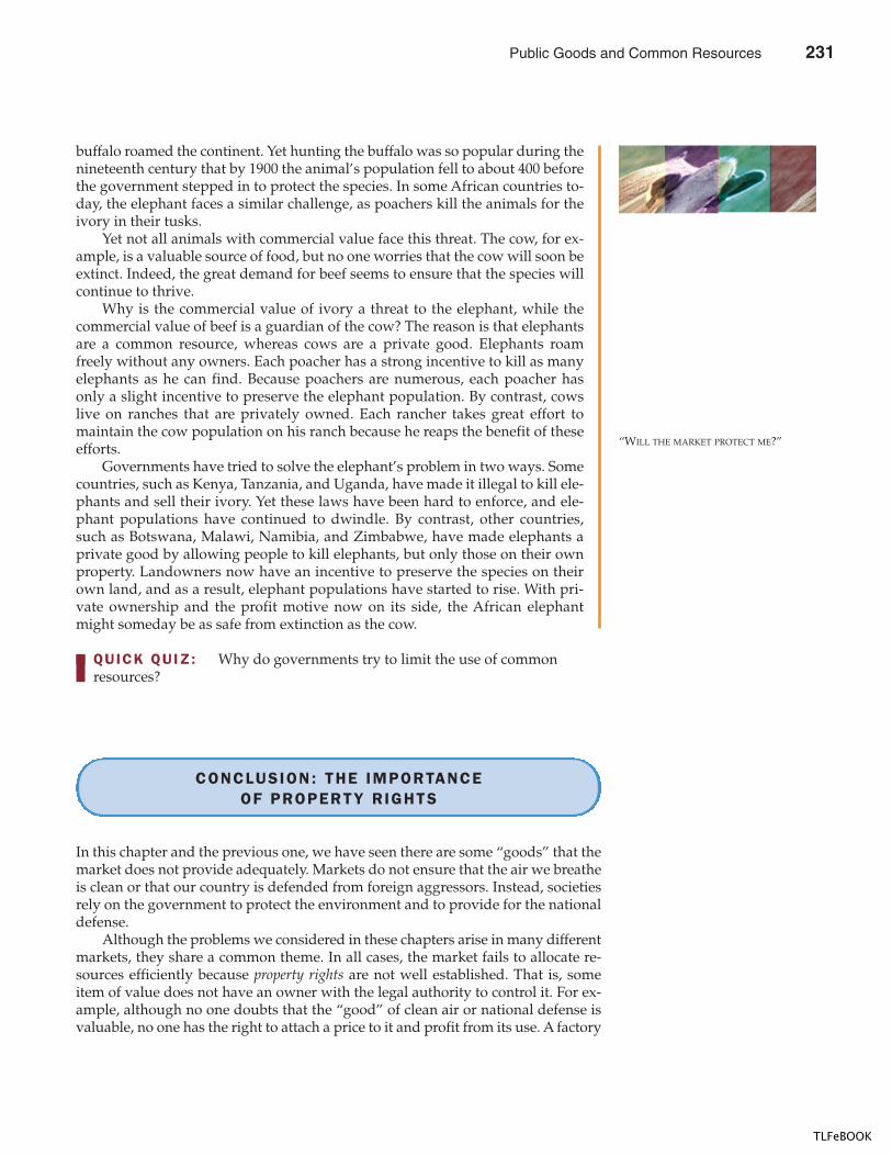
CHAPTER 11 PUBLIC GOODS AND COMMON RESOURCES 239
buffalo roamed the continent. Yet hunting the buffalo was so popular during thenineteenth century that by 1900 the animal’s population fell to about 400 beforethe government stepped in to protect the species. In some African countries to-day, the elephant faces a similar challenge, as poachers kill the animals for theivory in their tusks.
Yet not all animals with commercial value face this threat. The cow, for ex-ample, is a valuable source of food, but no one worries that the cow will soon beextinct. Indeed, the great demand for beef seems to ensure that the species willcontinue to thrive.
Why is the commercial value of ivory a threat to the elephant, while thecommercial value of beef is a guardian of the cow? The reason is that elephantsare a common resource, whereas cows are a private good. Elephants roamfreely without any owners. Each poacher has a strong incentive to kill as manyelephants as he can find. Because poachers are numerous, each poacher hasonly a slight incentive to preserve the elephant population. By contrast, cowslive on ranches that are privately owned. Each rancher takes great effort tomaintain the cow population on his ranch because he reaps the benefit of theseefforts.
Governments have tried to solve the elephant’s problem in two ways. Somecountries, such as Kenya, Tanzania, and Uganda, have made it illegal to kill ele-phants and sell their ivory. Yet these laws have been hard to enforce, and ele-phant populations have continued to dwindle. By contrast, other countries,such as Botswana, Malawi, Namibia, and Zimbabwe, have made elephants aprivate good by allowing people to kill elephants, but only those on their ownproperty. Landowners now have an incentive to preserve the species on theirown land, and as a result, elephant populations have started to rise. With pri-vate ownership and the profit motive now on its side, the African elephantmight someday be as safe from extinction as the cow.
QUICK QUIZ: Why do governments try to limit the use of common resources?
CONCLUSION: THE IMPORTANCEOF PROPERTY RIGHTS
In this chapter and the previous one, we have seen there are some “goods” that themarket does not provide adequately. Markets do not ensure that the air we breatheis clean or that our country is defended from foreign aggressors. Instead, societiesrely on the government to protect the environment and to provide for the nationaldefense.
Although the problems we considered in these chapters arise in many differentmarkets, they share a common theme. In all cases, the market fails to allocate re-sources efficiently because property rights are not well established. That is, someitem of value does not have an owner with the legal authority to control it. For ex-ample, although no one doubts that the “good” of clean air or national defense isvaluable, no one has the right to attach a price to it and profit from its use. A factory
“WILL THE MARKET PROTECT ME?”
Public Goods and Common Resources 231
TLFeBOOK
240 PART FOUR THE ECONOMICS OF THE PUBLIC SECTOR
pollutes too much because no one charges the factory for the pollution it emits. Themarket does not provide for national defense because no one can charge those whoare defended for the benefit they receive.
When the absence of property rights causes a market failure, the governmentcan potentially solve the problem. Sometimes, as in the sale of pollution permits,the solution is for the government to help define property rights and thereby un-leash market forces. Other times, as in the restriction on hunting seasons, the solu-tion is for the government to regulate private behavior. Still other times, as in theprovision of national defense, the solution is for the government to supply a goodthat the market fails to supply. In all cases, if the policy is well planned and wellrun, it can make the allocation of resources more efficient and thus raise economicwell-being.
� Goods differ in whether they are excludable andwhether they are rival. A good is excludable if it ispossible to prevent someone from using it. A good isrival if one person’s enjoyment of the good preventsother people from enjoying the same unit of the good.Markets work best for private goods, which are bothexcludable and rival. Markets do not work as well forother types of goods.
� Public goods are neither rival nor excludable.Examples of public goods include fireworks displays,national defense, and the creation of fundamentalknowledge. Because people are not charged for their use
of the public good, they have an incentive to free ridewhen the good is provided privately. Therefore,governments provide public goods, making theirdecision about the quantity based on cost-benefitanalysis.
� Common resources are rival but not excludable.Examples include common grazing land, clean air, andcongested roads. Because people are not charged fortheir use of common resources, they tend to use themexcessively. Therefore, governments try to limit the useof common resources.
Summar y
excludability, p. 226rivalry, p. 226private goods, p. 226
public goods, p. 226common resources, p. 226free rider, p. 228
cost-benefit analysis, p. 231Tragedy of the Commons, p. 234
Key Concepts
1. Explain what is meant by a good being “excludable.”Explain what is meant by a good being “rival.” Is apizza excludable? Is it rival?
2. Define and give an example of a public good. Canthe private market provide this good on its own?Explain.
3. What is cost-benefit analysis of public goods? Why is itimportant? Why is it hard?
4. Define and give an example of a common resource.Without government intervention, will people use thisgood too much or too little? Why?
Quest ions fo r Rev iew
232 Public Goods and Common Resources
TLFeBOOK
CHAPTER 11 PUBLIC GOODS AND COMMON RESOURCES 241
1. The text says that both public goods and commonresources involve externalities.a. Are the externalities associated with public goods
generally positive or negative? Use examples inyour answer. Is the free-market quantity of publicgoods generally greater or less than the efficientquantity?
b. Are the externalities associated with commonresources generally positive or negative? Useexamples in your answer. Is the free-market use ofcommon resources generally greater or less than theefficient use?
2. Think about the goods and services provided by yourlocal government.a. Using the classification in Figure 11-1, explain what
category each of the following goods falls into:� police protection� snow plowing� education� rural roads� city streets
b. Why do you think the government provides itemsthat are not public goods?
3. Charlie loves watching Teletubbies on his local public TVstation, but he never sends any money to support thestation during their fund-raising drives.a. What name do economists have for Charlie?b. How can the government solve the problem caused
by people like Charlie?c. Can you think of ways the private market can solve
this problem? How does the existence of cable TValter the situation?
4. The text states that private firms will not undertake theefficient amount of basic scientific research.a. Explain why this is so. In your answer, classify
basic research in one of the categories shown inFigure 11-1.
b. What sort of policy has the United States adoptedin response to this problem?
c. It is often argued that this policy increases thetechnological capability of American producersrelative to that of foreign firms. Is this argumentconsistent with your classification of basic researchin part (a)? (Hint: Can excludability apply to somepotential beneficiaries of a public good and notothers?)
5. Why is there litter along most highways but rarely inpeople’s yards?
6. The Washington, D.C., metro (subway) system chargeshigher fares during rush hours than during the rest ofthe day. Why might it do this?
7. Timber companies in the United States cut down manytrees on publicly owned land and many trees onprivately owned land. Discuss the likely efficiency oflogging on each type of land in the absence ofgovernment regulation. How do you think thegovernment should regulate logging on publicly ownedlands? Should similar regulations apply to privatelyowned land?
8. An Economist article (March 19, 1994) states: “In the pastdecade, most of the rich world’s fisheries have beenexploited to the point of near-exhaustion.” The articlecontinues with an analysis of the problem and adiscussion of possible private and government solutions:a. “Do not blame fishermen for overfishing. They are
behaving rationally, as they have always done.” Inwhat sense is “overfishing” rational for fishermen?
b. “A community, held together by ties of obligationand mutual self-interest, can manage a commonresource on its own.” Explain how suchmanagement can work in principle, and whatobstacles it faces in the real world.
c. “Until 1976 most world fish stocks were open to allcomers, making conservation almost impossible.Then an international agreement extended someaspects of [national] jurisdiction from 12 to 200miles offshore.” Using the concept of propertyrights, discuss how this agreement reduces thescope of the problem.
d. The article notes that many governments come tothe aid of suffering fishermen in ways thatencourage increased fishing. How do such policiesencourage a vicious cycle of overfishing?
e. “Only when fishermen believe they are assured along-term and exclusive right to a fishery are theylikely to manage it in the same far-sighted way asgood farmers manage their land.” Defend thisstatement.
f. What other policies to reduce overfishing might beconsidered?
9. In a market economy, information about the quality orfunction of goods and services is a valuable good in its
Prob lems and App l icat ions
Public Goods and Common Resources 233
TLFeBOOK
242 PART FOUR THE ECONOMICS OF THE PUBLIC SECTOR
own right. How does the private market provide thisinformation? Can you think of any way in which thegovernment plays a role in providing this information?
10. Do you think the Internet is a public good? Why orwhy not?
11. High-income people are willing to pay more than lower-income people to avoid the risk of death. For example,
they are more likely to pay for safety features on cars.Do you think cost-benefit analysts should take this factinto account when evaluating public projects? Consider,for instance, a rich town and a poor town, both of whichare considering the installation of a traffic light. Shouldthe rich town use a higher dollar value for a human lifein making this decision? Why or why not?
234 Public Goods and Common Resources
TLFeBOOK
IN THIS CHAPTERYOU WILL . . .
Cons ider thet radeof f between
ef f ic iency andequ i ty in the des ign
of a tax system
Learn a l te rnat iveways to judge the
equ i ty o f a taxsystem
Get an over v iew o fhow the U.S.
government ra isesand spends money
Examine theef f ic iency costs
of taxes
See why study ingtax inc idence is
cruc ia l fo reva luat ing tax
equ i ty
Al “Scarface” Capone, the notorious 1920s gangster and crime boss, was neverconvicted for his many violent crimes. Yet eventually he did go to jail—for tax eva-sion. He had neglected to heed Ben Franklin’s observation that “in this worldnothing is certain, but death and taxes.”
When Franklin made this claim in 1789, the average American paid less than5 percent of his income in taxes, and that remained true for the next hundredyears. Over the course of the twentieth century, however, taxes have become evermore important in the life of the typical person. Today, all taxes taken together—including personal income taxes, corporate income taxes, payroll taxes, sales taxes,and property taxes—use up about a third of the average American’s income. Inmany European countries, the tax bite is even larger.
Taxes are inevitable because we as citizens expect the government to provideus with various goods and services. The previous two chapters have started to
T H E D E S I G N O F
T H E T A X S Y S T E M
243
235
12
TLFeBOOK
244 PART FOUR THE ECONOMICS OF THE PUBLIC SECTOR
shed light on one of the Ten Principles of Economics from Chapter 1: The govern-ment can sometimes improve market outcomes. When the government remediesan externality (such as air pollution), provides a public good (such as national de-fense), or regulates the use of a common resource (such as fish in a public lake), itcan raise economic well-being. Yet the benefits of government come with costs. Forthe government to perform these and its many other functions, it needs to raiserevenue through taxation.
We began our study of taxation in earlier chapters, where we saw how a tax ona good affects supply and demand for that good. In Chapter 6 we saw that a tax re-duces the quantity sold in a market, and we examined how the burden of a tax isshared by buyers and sellers, depending on the elasticities of supply and demand.In Chapter 8 we examined how taxes affect economic well-being. We learned thattaxes cause deadweight losses: The reduction in consumer and producer surplus re-sulting from a tax exceeds the revenue raised by the government.
In this chapter we build on these lessons to discuss the design of a tax system.We begin with a financial overview of the U.S. government. When thinking aboutthe tax system, it is useful to know some basic facts about how the U.S. govern-ment raises and spends money. We then consider the fundamental principles oftaxation. Most people agree that taxes should impose as small a cost on society aspossible and that the burden of taxes should be distributed fairly. That is, the taxsystem should be both efficient and equitable. As we will see, however, stating thesegoals is easier than achieving them.
A FINANCIAL OVERVIEW OFTHE U.S. GOVERNMENT
How much of the nation’s income does the government take as taxes? Figure 12-1shows government revenue, including federal, state, and local governments, as apercentage of total income for the U.S. economy. It shows that, over time, the gov-ernment has taken a larger and larger share of total income. In 1902, the govern-ment collected 7 percent of total income; in 1998, it collected 32 percent. In otherwords, as the economy’s income has grown, the government has grown evenmore.
Table 12-1 compares the tax burden for several major countries, as measuredby the central government’s tax revenue as a percentage of the nation’s total in-come. The United States is in the middle of the pack. The U.S. tax burden is lowcompared to many European countries, but it is high compared to many other na-tions around the world. Poor countries, such as India and Pakistan, usually haverelatively low tax burdens. This fact is consistent with the evidence in Figure 12-1of a growing tax burden over time: As a nation gets richer, the government typi-cally takes a larger share of income in taxes.
The overall size of government tells only part of the story. Behind the total dol-lar figures lie thousands of individual decisions about taxes and spending. To un-derstand the government’s finances more fully, let’s look at how the total breaksdown into some broad categories.
236 The Design of the Tax System
TLFeBOOK
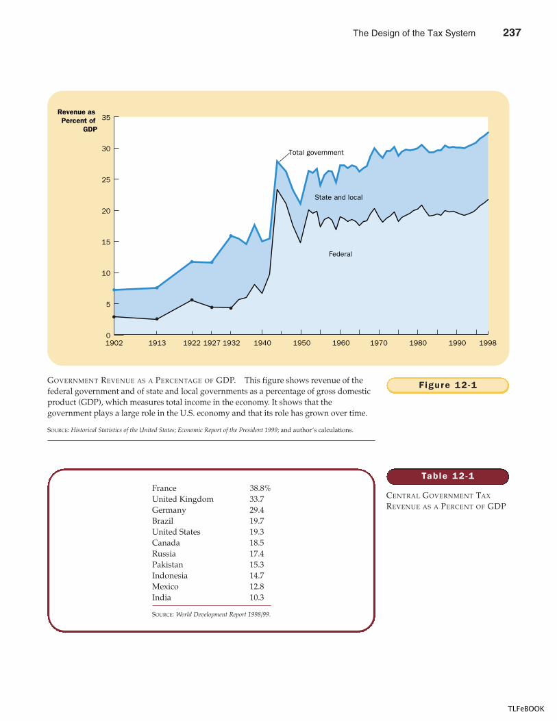
CHAPTER 12 THE DESIGN OF THE TAX SYSTEM 245
0
5
10
15
20
25
30
35
Federal
State and local
Revenue asPercent of
GDP
Total government
1902 1922 19271913 19401932 1970 1980 1990 19981950 1960
Figure 12 -1GOVERNMENT REVENUE AS A PERCENTAGE OF GDP. This figure shows revenue of thefederal government and of state and local governments as a percentage of gross domesticproduct (GDP), which measures total income in the economy. It shows that thegovernment plays a large role in the U.S. economy and that its role has grown over time.
SOURCE: Historical Statistics of the United States; Economic Report of the President 1999; and author’s calculations.
Table 12 -1
CENTRAL GOVERNMENT TAX
REVENUE AS A PERCENT OF GDP
France 38.8%United Kingdom 33.7Germany 29.4Brazil 19.7United States 19.3Canada 18.5Russia 17.4Pakistan 15.3Indonesia 14.7Mexico 12.8India 10.3
SOURCE: World Development Report 1998/99.
The Design of the Tax System 237
TLFeBOOK
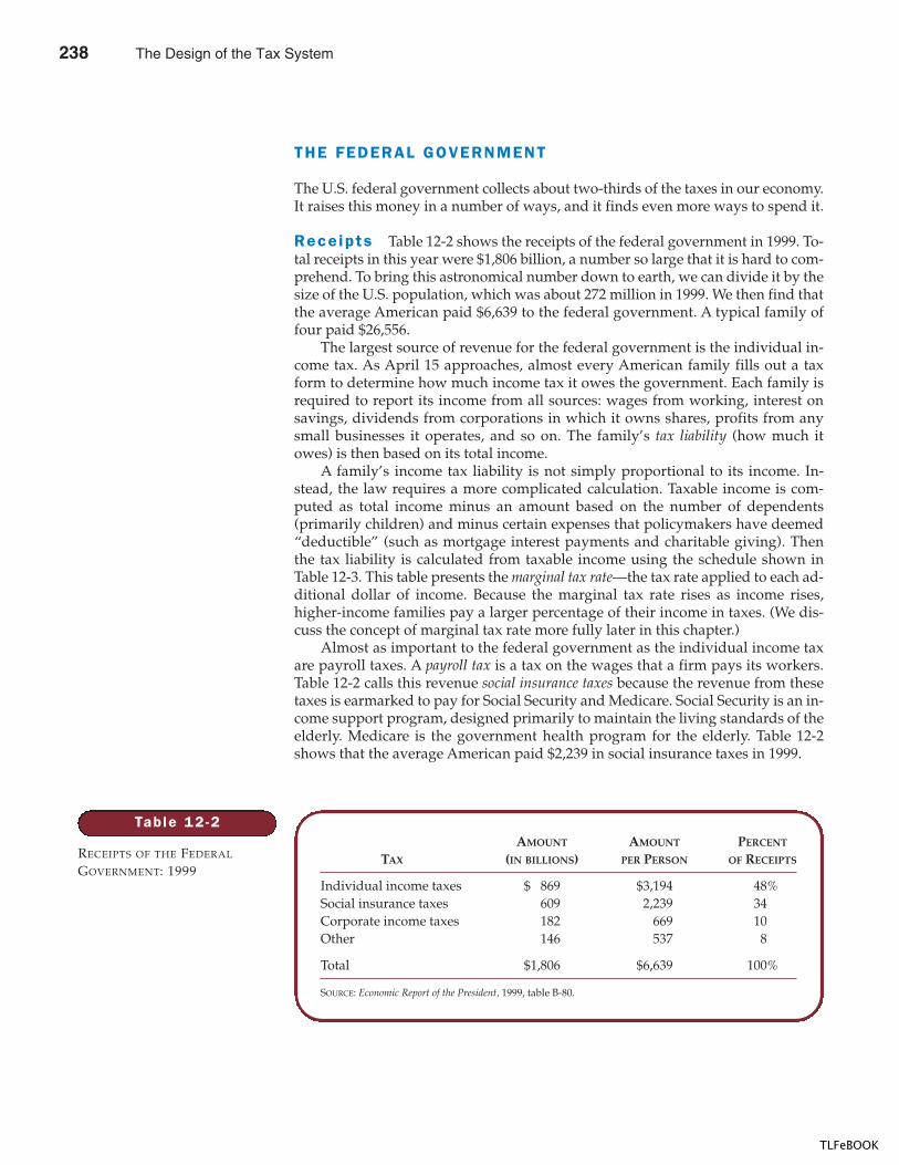
246 PART FOUR THE ECONOMICS OF THE PUBLIC SECTOR
THE FEDERAL GOVERNMENT
The U.S. federal government collects about two-thirds of the taxes in our economy.It raises this money in a number of ways, and it finds even more ways to spend it.
Receipts Table 12-2 shows the receipts of the federal government in 1999. To-tal receipts in this year were $1,806 billion, a number so large that it is hard to com-prehend. To bring this astronomical number down to earth, we can divide it by thesize of the U.S. population, which was about 272 million in 1999. We then find thatthe average American paid $6,639 to the federal government. A typical family offour paid $26,556.
The largest source of revenue for the federal government is the individual in-come tax. As April 15 approaches, almost every American family fills out a taxform to determine how much income tax it owes the government. Each family isrequired to report its income from all sources: wages from working, interest onsavings, dividends from corporations in which it owns shares, profits from anysmall businesses it operates, and so on. The family’s tax liability (how much itowes) is then based on its total income.
A family’s income tax liability is not simply proportional to its income. In-stead, the law requires a more complicated calculation. Taxable income is com-puted as total income minus an amount based on the number of dependents(primarily children) and minus certain expenses that policymakers have deemed“deductible” (such as mortgage interest payments and charitable giving). Thenthe tax liability is calculated from taxable income using the schedule shown inTable 12-3. This table presents the marginal tax rate—the tax rate applied to each ad-ditional dollar of income. Because the marginal tax rate rises as income rises,higher-income families pay a larger percentage of their income in taxes. (We dis-cuss the concept of marginal tax rate more fully later in this chapter.)
Almost as important to the federal government as the individual income taxare payroll taxes. A payroll tax is a tax on the wages that a firm pays its workers.Table 12-2 calls this revenue social insurance taxes because the revenue from thesetaxes is earmarked to pay for Social Security and Medicare. Social Security is an in-come support program, designed primarily to maintain the living standards of theelderly. Medicare is the government health program for the elderly. Table 12-2shows that the average American paid $2,239 in social insurance taxes in 1999.
Table 12 -2
RECEIPTS OF THE FEDERAL
GOVERNMENT: 1999
AMOUNT AMOUNT PERCENT
TAX (IN BILLIONS) PER PERSON OF RECEIPTS
Individual income taxes $ 869 $3,194 48%Social insurance taxes 609 2,239 34Corporate income taxes 182 669 10Other 146 537 8
Total $1,806 $6,639 100%
SOURCE: Economic Report of the President, 1999, table B-80.
238 The Design of the Tax System
TLFeBOOK
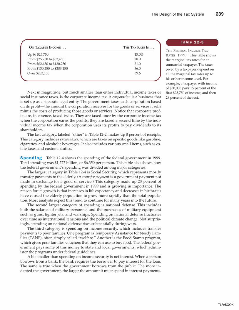
CHAPTER 12 THE DESIGN OF THE TAX SYSTEM 247
Next in magnitude, but much smaller than either individual income taxes orsocial insurance taxes, is the corporate income tax. A corporation is a business thatis set up as a separate legal entity. The government taxes each corporation basedon its profit—the amount the corporation receives for the goods or services it sellsminus the costs of producing those goods or services. Notice that corporate prof-its are, in essence, taxed twice. They are taxed once by the corporate income taxwhen the corporation earns the profits; they are taxed a second time by the indi-vidual income tax when the corporation uses its profits to pay dividends to itsshareholders.
The last category, labeled “other” in Table 12-2, makes up 8 percent of receipts.This category includes excise taxes, which are taxes on specific goods like gasoline,cigarettes, and alcoholic beverages. It also includes various small items, such as es-tate taxes and customs duties.
Spend ing Table 12-4 shows the spending of the federal government in 1999.Total spending was $1,727 billion, or $6,350 per person. This table also shows howthe federal government’s spending was divided among major categories.
The largest category in Table 12-4 is Social Security, which represents mostlytransfer payments to the elderly. (A transfer payment is a government payment notmade in exchange for a good or service.) This category made up 23 percent ofspending by the federal government in 1999 and is growing in importance. Thereason for its growth is that increases in life expectancy and decreases in birthrateshave caused the elderly population to grow more rapidly than the total popula-tion. Most analysts expect this trend to continue for many years into the future.
The second largest category of spending is national defense. This includesboth the salaries of military personnel and the purchases of military equipmentsuch as guns, fighter jets, and warships. Spending on national defense fluctuatesover time as international tensions and the political climate change. Not surpris-ingly, spending on national defense rises substantially during wars.
The third category is spending on income security, which includes transferpayments to poor families. One program is Temporary Assistance for Needy Fam-ilies (TANF), often simply called “welfare.” Another is the Food Stamp program,which gives poor families vouchers that they can use to buy food. The federal gov-ernment pays some of this money to state and local governments, which admin-ister the programs under federal guidelines.
A bit smaller than spending on income security is net interest. When a personborrows from a bank, the bank requires the borrower to pay interest for the loan.The same is true when the government borrows from the public. The more in-debted the government, the larger the amount it must spend in interest payments.
Table 12 -3
THE FEDERAL INCOME TAX
RATES: 1999. This table showsthe marginal tax rates for anunmarried taxpayer. The taxesowed by a taxpayer depend onall the marginal tax rates up tohis or her income level. Forexample, a taxpayer with incomeof $50,000 pays 15 percent of thefirst $25,750 of income, and then28 percent of the rest.
ON TAXABLE INCOME . . . THE TAX RATE IS . . .
Up to $25,750 15.0%From $25,750 to $62,450 28.0From $62,450 to $130,250 31.0From $130,250 to $283,150 36.0Over $283,150 39.6
The Design of the Tax System 239
TLFeBOOK
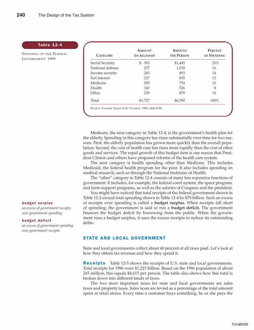
248 PART FOUR THE ECONOMICS OF THE PUBLIC SECTOR
Medicare, the next category in Table 12-4, is the government’s health plan forthe elderly. Spending in this category has risen substantially over time for two rea-sons. First, the elderly population has grown more quickly than the overall popu-lation. Second, the cost of health care has risen more rapidly than the cost of othergoods and services. The rapid growth of this budget item is one reason that Presi-dent Clinton and others have proposed reforms of the health care system.
The next category is health spending other than Medicare. This includesMedicaid, the federal health program for the poor. It also includes spending onmedical research, such as through the National Institutes of Health.
The “other” category in Table 12-4 consists of many less expensive functions ofgovernment. It includes, for example, the federal court system, the space program,and farm-support programs, as well as the salaries of Congress and the president.
You might have noticed that total receipts of the federal government shown inTable 12-2 exceed total spending shown in Table 12-4 by $79 billion. Such an excessof receipts over spending is called a budget surplus. When receipts fall shortof spending, the government is said to run a budget deficit. The governmentfinances the budget deficit by borrowing from the public. When the govern-ment runs a budget surplus, it uses the excess receipts to reduce its outstandingdebts.
STATE AND LOCAL GOVERNMENT
State and local governments collect about 40 percent of all taxes paid. Let’s look athow they obtain tax revenue and how they spend it.
Rece ipts Table 12-5 shows the receipts of U.S. state and local governments.Total receipts for 1996 were $1,223 billion. Based on the 1996 population of about265 million, this equals $4,615 per person. The table also shows how this total isbroken down into different kinds of taxes.
The two most important taxes for state and local governments are salestaxes and property taxes. Sales taxes are levied as a percentage of the total amountspent at retail stores. Every time a customer buys something, he or she pays the
Table 12 -4
SPENDING OF THE FEDERAL
GOVERNMENT: 1999
AMOUNT AMOUNT PERCENT
CATEGORY (IN BILLIONS) PER PERSON OF SPENDING
Social Security $ 393 $1,445 23%National defense 277 1,018 16Income security 243 893 14Net interest 227 835 13Medicare 205 754 12Health 143 526 8Other 239 879 14
Total $1,727 $6,350 100%
SOURCE: Economic Report of the President, 1999, table B-80.
budget surp lusan excess of government receiptsover government spending
budget def ic i tan excess of government spendingover government receipts
240 The Design of the Tax System
TLFeBOOK
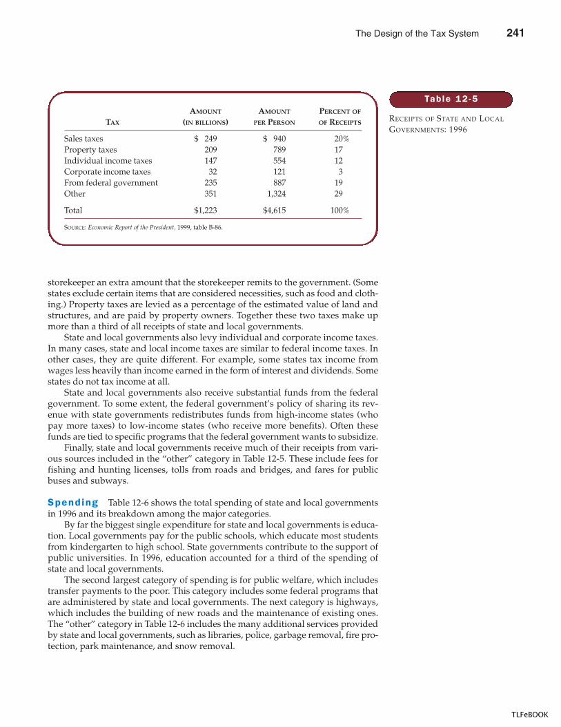
CHAPTER 12 THE DESIGN OF THE TAX SYSTEM 249
storekeeper an extra amount that the storekeeper remits to the government. (Somestates exclude certain items that are considered necessities, such as food and cloth-ing.) Property taxes are levied as a percentage of the estimated value of land andstructures, and are paid by property owners. Together these two taxes make upmore than a third of all receipts of state and local governments.
State and local governments also levy individual and corporate income taxes.In many cases, state and local income taxes are similar to federal income taxes. Inother cases, they are quite different. For example, some states tax income fromwages less heavily than income earned in the form of interest and dividends. Somestates do not tax income at all.
State and local governments also receive substantial funds from the federalgovernment. To some extent, the federal government’s policy of sharing its rev-enue with state governments redistributes funds from high-income states (whopay more taxes) to low-income states (who receive more benefits). Often thesefunds are tied to specific programs that the federal government wants to subsidize.
Finally, state and local governments receive much of their receipts from vari-ous sources included in the “other” category in Table 12-5. These include fees forfishing and hunting licenses, tolls from roads and bridges, and fares for publicbuses and subways.
Spending Table 12-6 shows the total spending of state and local governmentsin 1996 and its breakdown among the major categories.
By far the biggest single expenditure for state and local governments is educa-tion. Local governments pay for the public schools, which educate most studentsfrom kindergarten to high school. State governments contribute to the support ofpublic universities. In 1996, education accounted for a third of the spending ofstate and local governments.
The second largest category of spending is for public welfare, which includestransfer payments to the poor. This category includes some federal programs thatare administered by state and local governments. The next category is highways,which includes the building of new roads and the maintenance of existing ones.The “other” category in Table 12-6 includes the many additional services providedby state and local governments, such as libraries, police, garbage removal, fire pro-tection, park maintenance, and snow removal.
Table 12 -5
RECEIPTS OF STATE AND LOCAL
GOVERNMENTS: 1996
AMOUNT AMOUNT PERCENT OF
TAX (IN BILLIONS) PER PERSON OF RECEIPTS
Sales taxes $ 249 $ 940 20%Property taxes 209 789 17Individual income taxes 147 554 12Corporate income taxes 32 121 3From federal government 235 887 19Other 351 1,324 29
Total $1,223 $4,615 100%
SOURCE: Economic Report of the President, 1999, table B-86.
The Design of the Tax System 241
TLFeBOOK
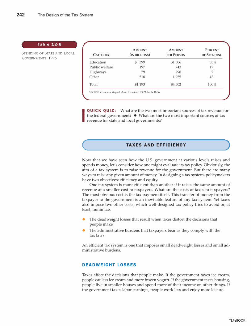
250 PART FOUR THE ECONOMICS OF THE PUBLIC SECTOR
QUICK QUIZ: What are the two most important sources of tax revenue for the federal government? � What are the two most important sources of tax revenue for state and local governments?
TAXES AND EFFICIENCY
Now that we have seen how the U.S. government at various levels raises andspends money, let’s consider how one might evaluate its tax policy. Obviously, theaim of a tax system is to raise revenue for the government. But there are manyways to raise any given amount of money. In designing a tax system, policymakershave two objectives: efficiency and equity.
One tax system is more efficient than another if it raises the same amount ofrevenue at a smaller cost to taxpayers. What are the costs of taxes to taxpayers?The most obvious cost is the tax payment itself. This transfer of money from thetaxpayer to the government is an inevitable feature of any tax system. Yet taxesalso impose two other costs, which well-designed tax policy tries to avoid or, atleast, minimize:
� The deadweight losses that result when taxes distort the decisions thatpeople make
� The administrative burdens that taxpayers bear as they comply with thetax laws
An efficient tax system is one that imposes small deadweight losses and small ad-ministrative burdens.
DEADWEIGHT LOSSES
Taxes affect the decisions that people make. If the government taxes ice cream,people eat less ice cream and more frozen yogurt. If the government taxes housing,people live in smaller houses and spend more of their income on other things. Ifthe government taxes labor earnings, people work less and enjoy more leisure.
Table 12 -6
SPENDING OF STATE AND LOCAL
GOVERNMENTS: 1996
AMOUNT AMOUNT PERCENT
CATEGORY (IN BILLIONS) PER PERSON OF SPENDING
Education $ 399 $1,506 33%Public welfare 197 743 17Highways 79 298 7Other 518 1,955 43
Total $1,193 $4,502 100%
SOURCE: Economic Report of the President, 1999, table B-86.
242 The Design of the Tax System
TLFeBOOK
CHAPTER 12 THE DESIGN OF THE TAX SYSTEM 251
CASE STUDY SHOULD INCOME OR CONSUMPTION BE TAXED?
When taxes induce people to change their behavior—such as inducing Jane tobuy less pizza—the taxes cause deadweight losses and make the allocation ofresources less efficient. As we have already seen, much government revenuecomes from the individual income tax. In a case study in Chapter 8, we dis-cussed how this tax discourages people from working as hard as they otherwisemight. Another inefficiency caused by this tax is that it discourages people fromsaving.
Consider a person 25 years old who is considering saving $100. If he putsthis money in a savings account that earns 8 percent and leaves it there, hewould have $2,172 when he retires at age 65. Yet if the government taxes one-fourth of his interest income each year, the effective interest rate is only 6 per-cent. After 40 years of earning 6 percent, the $100 grows to only $1,029, less thanhalf of what it would have been without taxation. Thus, because interest incomeis taxed, saving is much less attractive.
Some economists advocate eliminating the current tax system’s disincentivetoward saving by changing the basis of taxation. Rather than taxing the amountof income that people earn, the government could tax the amount that peoplespend. Under this proposal, all income that is saved would not be taxed until thesaving is later spent. This alternative system, called a consumption tax, wouldnot distort people’s saving decisions.
This idea has some support from policymakers. Representative Bill Archer,who in 1995 became chairman of the powerful House Ways and Means
Because taxes distort incentives, they entail deadweight losses. As we first dis-cussed in Chapter 8, the deadweight loss of a tax is the reduction in economic well-being of taxpayers in excess of the amount of revenue raised by the government.The deadweight loss is the inefficiency that a tax creates as people allocate re-sources according to the tax incentive rather than the true costs and benefits of thegoods and services that they buy and sell.
To recall how taxes cause deadweight losses, consider an example. Supposethat Joe places an $8 value on a pizza, and Jane places a $6 value on it. If there is notax on pizza, the price of pizza will reflect the cost of making it. Let’s suppose thatthe price of pizza is $5, so both Joe and Jane choose to buy one. Both consumers getsome surplus of value over the amount paid. Joe gets consumer surplus of $3, andJane gets consumer surplus of $1. Total surplus is $4.
Now suppose that the government levies a $2 tax on pizza and the price ofpizza rises to $7. Joe still buys a pizza, but now he has consumer surplus of only$1. Jane now decides not to buy a pizza because its price is higher than its value toher. The government collects tax revenue of $2 on Joe’s pizza. Total consumersurplus has fallen by $3 (from $4 to $1). Because total surplus has fallen by morethan the tax revenue, the tax has a deadweight loss. In this case, the deadweightloss is $1.
Notice that the deadweight loss comes not from Joe, the person who pays thetax, but from Jane, the person who doesn’t. The reduction of $2 in Joe’s surplus ex-actly offsets the amount of revenue the government collects. The deadweight lossarises because the tax causes Jane to alter her behavior. When the tax raises theprice of pizza, Jane is worse off, and yet there is no offsetting revenue to the gov-ernment. This reduction in Jane’s welfare is the deadweight loss of the tax.
“I was gonna fix the place up, butif I did the city would just raisemy taxes!”
The Design of the Tax System 243
TLFeBOOK
252 PART FOUR THE ECONOMICS OF THE PUBLIC SECTOR
Committee, has advocated replacing the current income tax system with a con-sumption tax. Moreover, various provisions of the current tax code alreadymake the tax system a bit like a consumption tax. Taxpayers can put a limitedamount of their saving into special accounts—such as Individual RetirementAccounts, Keogh plans, and 401(k) plans—that escape taxation until the moneyis withdrawn at retirement. For people who do most of their saving throughthese retirement accounts, their tax bill is, in effect, based on their consumptionrather than their income.
ADMINISTRATIVE BURDEN
If you ask the typical person on April 15 for an opinion about the tax system, youmight hear about the headache of filling out tax forms. The administrative burdenof any tax system is part of the inefficiency it creates. This burden includes notonly the time spent in early April filling out forms but also the time spentthroughout the year keeping records for tax purposes and the resources the gov-ernment has to use to enforce the tax laws.
Many taxpayers—especially those in higher tax brackets—hire tax lawyersand accountants to help them with their taxes. These experts in the complex taxlaws fill out the tax forms for their clients and help clients arrange their affairs in away that reduces the amount of taxes owed. This behavior is legal tax avoidance,which is different from illegal tax evasion.
Critics of our tax system say that these advisers help their clients avoid taxesby abusing some of the detailed provisions of the tax code, often dubbed “loop-holes.” In some cases, loopholes are congressional mistakes: They arise from am-biguities or omissions in the tax laws. More often, they arise because Congress haschosen to give special treatment to specific types of behavior. For example, the U.S.federal tax code gives preferential treatment to investors in municipal bonds be-cause Congress wanted to make it easier for state and local governments to borrowmoney. To some extent, this provision benefits states and localities; to some extent,it benefits high-income taxpayers. Most loopholes are well known by those in Con-gress who make tax policy, but what looks like a loophole to one taxpayer maylook like a justifiable tax deduction to another.
The resources devoted to complying with the tax laws are a type of dead-weight loss. The government gets only the amount of taxes paid. By contrast, thetaxpayer loses not only this amount but also the time and money spent docu-menting, computing, and avoiding taxes.
The administrative burden of the tax system could be reduced by simplifyingthe tax laws. Yet simplification is often politically difficult. Most people are readyto simplify the tax code by eliminating the loopholes that benefit others, yet feware eager to give up the loopholes that they use. In the end, the complexity of thetax law results from the political process as various taxpayers with their own spe-cial interests lobby for their causes.
MARGINAL TAX RATES VERSUS AVERAGE TAX RATES
When discussing the efficiency and equity of income taxes, economists distinguishbetween two notions of the tax rate: the average and the marginal. The average taxrate is total taxes paid divided by total income. The marginal tax rate is the extrataxes paid on an additional dollar of income.
average tax ratetotal taxes paid divided by totalincome
marg ina l tax ratethe extra taxes paid on an additionaldollar of income
244 The Design of the Tax System
TLFeBOOK
CHAPTER 12 THE DESIGN OF THE TAX SYSTEM 253
For example, suppose that the government taxes 20 percent of the first $50,000of income and 50 percent of all income above $50,000. Under this tax, a person whomakes $60,000 pays a tax of $15,000. (The tax equals 0.20 � $50,000 plus 0.50 �$10,000.) For this person, the average tax rate is $15,000/$60,000, or 25 percent. But
PEOPLE RUNNING SMALL BUSINESSES ARE
most aware of the administrative bur-den of the tax system. Small firms mustcomply with many of the same laws aslarge ones. Yet, because of their size,compliance can take a much larger frac-tion of their revenue. According to onestudy, the administrative burden is tentimes larger for small firms than forlarge firms. The following article de-scribes some of these costs.
O b e y i n g t h e Ta x L a w s :S m a l l B u s i n e s s ’s B u r d e n
BY ROBERT D. HERSHEY, JR.In the grand scheme of a federal systemthat collects more than $1 trillion a year,Dante’s Restaurant, Inc., a modestthree-city chain in Pennsylvania, countsfor little.
But to people like Lewis Kamin,Dante’s controller, the Internal RevenueCode is a year-round headache. Thereare the biweekly remittances of SocialSecurity and withheld income tax, quar-terly reports of payroll and unem-ployment taxes, quarterly estimatedcorporate income taxes, and, of course,the maintaining of various records,
including tips, W-4s for withholding, andI-9 citizenship forms.
All this doesn’t count the ubiquitousstate and local levies that in Dante’scase are complicated because liquor-license considerations mean each of itsten restaurants must be separatelyincorporated.
“There is a lot to watch, a lot toworry about,” Mr. Kamin grumbled. . . .
This is the real-world side of Ameri-can taxation, the federal chunk of whichis a system based on a monumentallycomplex set of laws and regulations thatwas just one-third its current size whenJimmy Carter called it “a disgrace to thehuman race.”
The code is administered by a115,000-member Internal Revenue Ser-vice army with a $7 billion budget. Butthat amount is dwarfed by what taxpay-ers themselves spend on meeting theirobligations.
Estimates of what it costs Americanbusinesses to comply with federal taxlaw reach into the hundreds of billions ofdollars a year. . . . Big companies are un-der almost continuous audit. The 1992return for one giant company ran to21,000 pages and 30 volumes. Butthe heaviest burden by far falls on smallbusiness.
In fact, according to Arthur P. Hall, asenior fellow at The Tax Foundation, thelocal hardware store, delicatessen, orgas station with assets of less than $1million—a category embracing 90 per-cent of the nation’s corporations—spends $390 for each $100 it sends toWashington. Put another way, the gov-ernment got just $4.1 billion from these
businesses in 1990, compared with the$15.9 billion they spent producing thebasic corporate forms, the 1120 and1120S.
“What this means is that the cor-porate income tax is a very inefficientrevenue source for the federal govern-ment,” Mr. Hall said. . . .
Although complaints about the taxsystem are often aimed at the I.R.S.,businesspeople and policymakers gener-ally contend that the real fault lies withCongress and its frequent, often well-intentioned tinkering with the law. Theresulting complexity is taking an ever-mounting toll on respect for the system,and thereby undermines the willingnessof even the best-intentioned taxpayer tofigure out what he or she should pay. . . .
Since 1981, Washington has putten major tax laws on the books, gener-ating changes whose cumulative effect“is pretty staggering for the small busi-nessperson,” said Edward Koos, a tax-policy lawyer at the Small BusinessAdministration.
Harold Apolinsky of the Small Busi-ness Council says 9,371 code sectionshave been amended since 1981, a totalthat owes much to the lobbying andcampaign contributions of the powerful.“It appears to me that small businessjust has no clout,” Mr. Apolinsky said.“Big business tolerates it,” he added,referring to the resulting complexity.“Small business really can’t.”
SOURCE: The New York Times, January 30, 1994,Business Section, p. 4.
IN THE NEWS
Small Business andthe Tax Laws
The Design of the Tax System 245
TLFeBOOK
254 PART FOUR THE ECONOMICS OF THE PUBLIC SECTOR
the marginal tax rate is 50 percent because the amount of the tax would rise by$0.50 if the taxpayer earned an additional dollar.
The marginal and average tax rates each contain a useful piece of information.If we are trying to gauge the sacrifice made by a taxpayer, the average tax rate ismore appropriate because it measures the fraction of income paid in taxes. By con-trast, if we are trying to gauge how much the tax system distorts incentives, themarginal tax rate is more meaningful. One of the Ten Principles of Economics inChapter 1 is that rational people think at the margin. A corollary to this principleis that the marginal tax rate measures how much the tax system discourages peo-ple from working hard. It is the marginal tax rate, therefore, that determines thedeadweight loss of an income tax.
LUMP-SUM TAXES
Suppose the government imposes a tax of $4,000 on everyone. That is, everyoneowes the same amount, regardless of earnings or any actions that a person mighttake. Such a tax is called a lump-sum tax.
A lump-sum tax shows clearly the difference between average and marginaltax rates. For a taxpayer with income of $20,000, the average tax rate of a $4,000lump-sum tax is 20 percent; for a taxpayer with income of $40,000, the average taxrate is 10 percent. For both taxpayers, the marginal tax rate is zero because an ad-ditional dollar of income would not change the amount of tax owed.
A lump-sum tax is the most efficient tax possible. Because a person’s decisionsdo not alter the amount owed, the tax does not distort incentives and, therefore,does not cause deadweight losses. Because everyone can easily compute theamount owed and because there is no benefit to hiring tax lawyers and accoun-tants, the lump-sum tax imposes a minimal administrative burden on taxpayers.
If lump-sum taxes are so efficient, why do we rarely observe them in the realworld? The reason is that efficiency is only one goal of the tax system. A lump-sumtax would take the same amount from the poor and the rich, an outcome most peo-ple would view as unfair. To understand the tax systems that we observe, we musttherefore consider the other major goal of tax policy: equity.
QUICK QUIZ: What is meant by the efficiency of a tax system? � What can make a tax system inefficient?
TAXES AND EQUITY
Ever since American colonists dumped imported tea into Boston harbor to protesthigh British taxes, tax policy has generated some of the most heated debates inAmerican politics. The heat is rarely fueled by questions of efficiency. Instead, itarises from disagreements over how the tax burden should be distributed. SenatorRussell Long once mimicked the public debate with this ditty:
lump-sum taxa tax that is the same amount forevery person
246 The Design of the Tax System
TLFeBOOK
CHAPTER 12 THE DESIGN OF THE TAX SYSTEM 255
Don’t tax you.Don’t tax me.Tax that fella behind the tree.
Of course, if we are to rely on the government to provide some of the goods andservices we want, taxes must fall on someone. In this section we consider the eq-uity of a tax system. How should the burden of taxes be divided among the popu-lation? How do we evaluate whether a tax system is fair? Everyone agrees that thetax system should be equitable, but there is much disagreement about what equitymeans and how the equity of a tax system can be judged.
THE BENEFITS PRINCIPLE
One principle of taxation, called the benefits principle, states that people shouldpay taxes based on the benefits they receive from government services. This prin-ciple tries to make public goods similar to private goods. It seems fair that a per-son who often goes to the movies pays more in total for movie tickets than aperson who rarely goes. Similarly, a person who gets great benefit from a publicgood should pay more for it than a person who gets little benefit.
The gasoline tax, for instance, is sometimes justified using the benefits princi-ple. In some states, revenues from the gasoline tax are used to build and maintainroads. Because those who buy gasoline are the same people who use the roads, thegasoline tax might be viewed as a fair way to pay for this government service.
The benefits principle can also be used to argue that wealthy citizens shouldpay higher taxes than poorer ones. Why? Simply because the wealthy benefit morefrom public services. Consider, for example, the benefits of police protection fromtheft. Citizens with much to protect get greater benefit from police than do thosewith less to protect. Therefore, according to the benefits principle, the wealthyshould contribute more than the poor to the cost of maintaining the police force.The same argument can be used for many other public services, such as fire pro-tection, national defense, and the court system.
It is even possible to use the benefits principle to argue for antipoverty pro-grams funded by taxes on the wealthy. As we discussed in Chapter 11, people pre-fer living in a society without poverty, suggesting that antipoverty programs are apublic good. If the wealthy place a greater dollar value on this public good thanmembers of the middle class do, perhaps just because the wealthy have more tospend, then, according to the benefits principle, they should be taxed more heav-ily to pay for these programs.
THE ABIL ITY -TO-PAY PRINCIPLE
Another way to evaluate the equity of a tax system is called the ability-to-payprinciple, which states that taxes should be levied on a person according to howwell that person can shoulder the burden. This principle is sometimes justified bythe claim that all citizens should make an “equal sacrifice” to support the govern-ment. The magnitude of a person’s sacrifice, however, depends not only on thesize of his tax payment but also on his income and other circumstances. A $1,000tax paid by a poor person may require a larger sacrifice than a $10,000 tax paid bya rich one.
benef i ts p r inc ip lethe idea that people should pay taxesbased on the benefits they receivefrom government services
abi l i ty - to -pay pr inc ip lethe idea that taxes should be leviedon a person according to how wellthat person can shoulder the burden
The Design of the Tax System 247
TLFeBOOK
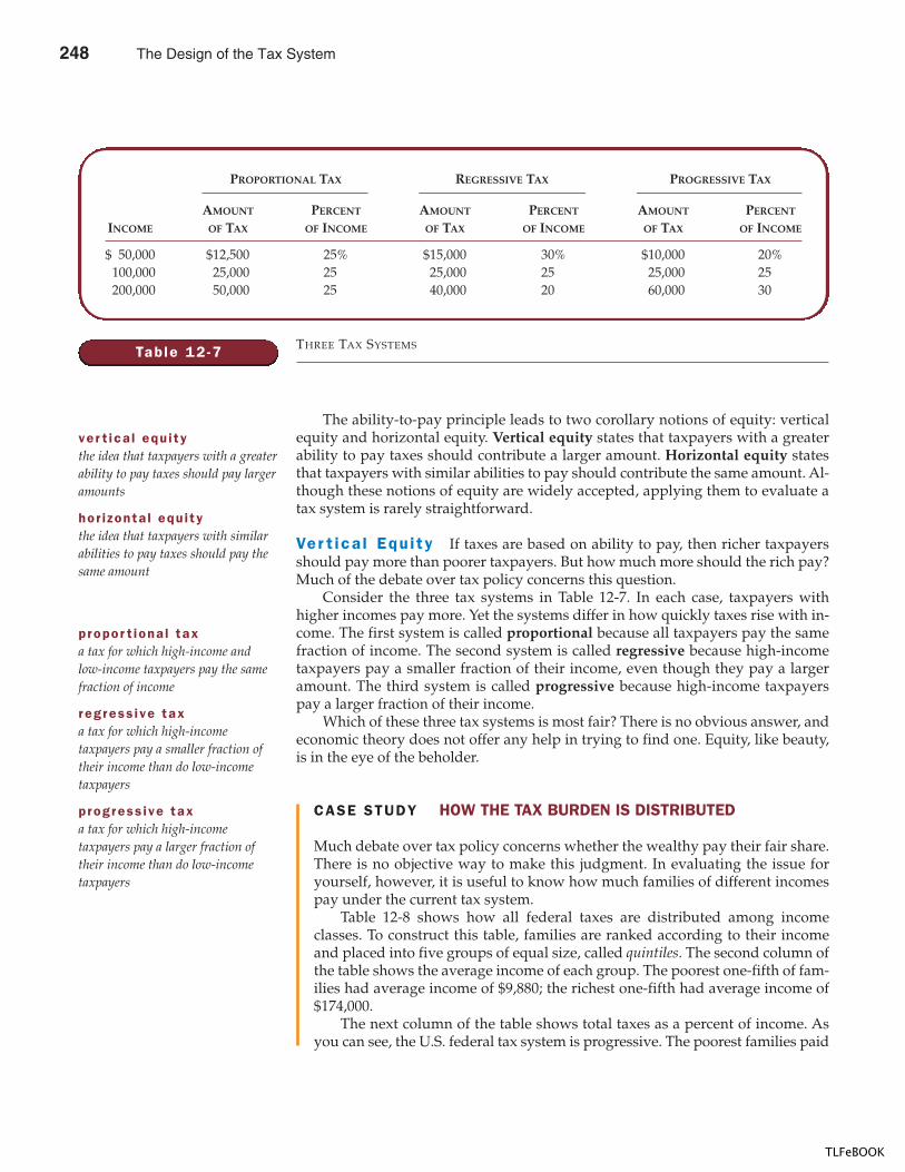
256 PART FOUR THE ECONOMICS OF THE PUBLIC SECTOR
CASE STUDY HOW THE TAX BURDEN IS DISTRIBUTED
Much debate over tax policy concerns whether the wealthy pay their fair share.There is no objective way to make this judgment. In evaluating the issue foryourself, however, it is useful to know how much families of different incomespay under the current tax system.
Table 12-8 shows how all federal taxes are distributed among incomeclasses. To construct this table, families are ranked according to their incomeand placed into five groups of equal size, called quintiles. The second column ofthe table shows the average income of each group. The poorest one-fifth of fam-ilies had average income of $9,880; the richest one-fifth had average income of$174,000.
The next column of the table shows total taxes as a percent of income. Asyou can see, the U.S. federal tax system is progressive. The poorest families paid
The ability-to-pay principle leads to two corollary notions of equity: verticalequity and horizontal equity. Vertical equity states that taxpayers with a greaterability to pay taxes should contribute a larger amount. Horizontal equity statesthat taxpayers with similar abilities to pay should contribute the same amount. Al-though these notions of equity are widely accepted, applying them to evaluate atax system is rarely straightforward.
Ver t ica l Equ i ty If taxes are based on ability to pay, then richer taxpayersshould pay more than poorer taxpayers. But how much more should the rich pay?Much of the debate over tax policy concerns this question.
Consider the three tax systems in Table 12-7. In each case, taxpayers withhigher incomes pay more. Yet the systems differ in how quickly taxes rise with in-come. The first system is called proportional because all taxpayers pay the samefraction of income. The second system is called regressive because high-incometaxpayers pay a smaller fraction of their income, even though they pay a largeramount. The third system is called progressive because high-income taxpayerspay a larger fraction of their income.
Which of these three tax systems is most fair? There is no obvious answer, andeconomic theory does not offer any help in trying to find one. Equity, like beauty,is in the eye of the beholder.
ver t ica l equ i tythe idea that taxpayers with a greaterability to pay taxes should pay largeramounts
hor i zonta l equ i tythe idea that taxpayers with similarabilities to pay taxes should pay thesame amount
Table 12 -7
PROPORTIONAL TAX REGRESSIVE TAX PROGRESSIVE TAX
AMOUNT PERCENT AMOUNT PERCENT AMOUNT PERCENT
INCOME OF TAX OF INCOME OF TAX OF INCOME OF TAX OF INCOME
$ 50,000 $12,500 25% $15,000 30% $10,000 20%100,000 25,000 25 25,000 25 25,000 25200,000 50,000 25 40,000 20 60,000 30
THREE TAX SYSTEMS
propor t iona l taxa tax for which high-income andlow-income taxpayers pay the samefraction of income
r egress ive taxa tax for which high-incometaxpayers pay a smaller fraction oftheir income than do low-incometaxpayers
progress ive taxa tax for which high-incometaxpayers pay a larger fraction oftheir income than do low-incometaxpayers
248 The Design of the Tax System
TLFeBOOK
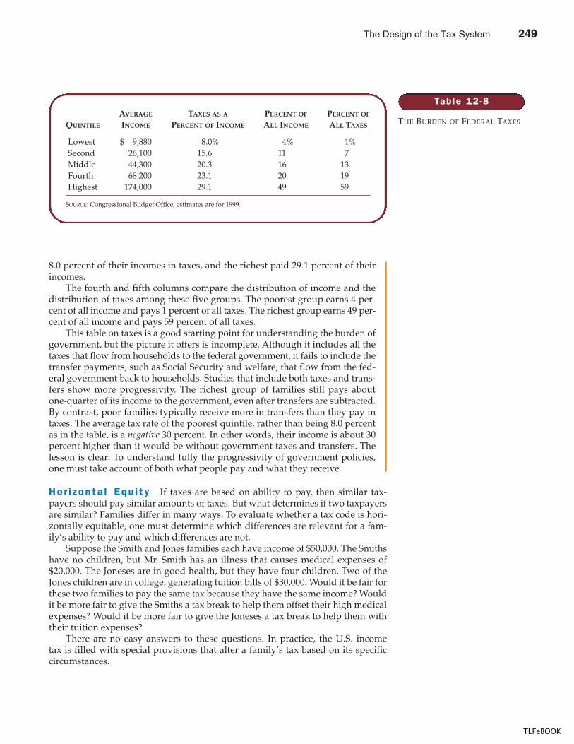
CHAPTER 12 THE DESIGN OF THE TAX SYSTEM 257
8.0 percent of their incomes in taxes, and the richest paid 29.1 percent of theirincomes.
The fourth and fifth columns compare the distribution of income and thedistribution of taxes among these five groups. The poorest group earns 4 per-cent of all income and pays 1 percent of all taxes. The richest group earns 49 per-cent of all income and pays 59 percent of all taxes.
This table on taxes is a good starting point for understanding the burden ofgovernment, but the picture it offers is incomplete. Although it includes all thetaxes that flow from households to the federal government, it fails to include thetransfer payments, such as Social Security and welfare, that flow from the fed-eral government back to households. Studies that include both taxes and trans-fers show more progressivity. The richest group of families still pays aboutone-quarter of its income to the government, even after transfers are subtracted.By contrast, poor families typically receive more in transfers than they pay intaxes. The average tax rate of the poorest quintile, rather than being 8.0 percentas in the table, is a negative 30 percent. In other words, their income is about 30percent higher than it would be without government taxes and transfers. Thelesson is clear: To understand fully the progressivity of government policies,one must take account of both what people pay and what they receive.
Hor i zonta l Equ i ty If taxes are based on ability to pay, then similar tax-payers should pay similar amounts of taxes. But what determines if two taxpayersare similar? Families differ in many ways. To evaluate whether a tax code is hori-zontally equitable, one must determine which differences are relevant for a fam-ily’s ability to pay and which differences are not.
Suppose the Smith and Jones families each have income of $50,000. The Smithshave no children, but Mr. Smith has an illness that causes medical expenses of$20,000. The Joneses are in good health, but they have four children. Two of theJones children are in college, generating tuition bills of $30,000. Would it be fair forthese two families to pay the same tax because they have the same income? Wouldit be more fair to give the Smiths a tax break to help them offset their high medicalexpenses? Would it be more fair to give the Joneses a tax break to help them withtheir tuition expenses?
There are no easy answers to these questions. In practice, the U.S. incometax is filled with special provisions that alter a family’s tax based on its specificcircumstances.
Table 12 -8
THE BURDEN OF FEDERAL TAXESAVERAGE TAXES AS A PERCENT OF PERCENT OF
QUINTILE INCOME PERCENT OF INCOME ALL INCOME ALL TAXES
Lowest $ 9,880 8.0% 4% 1%Second 26,100 15.6 11 7Middle 44,300 20.3 16 13Fourth 68,200 23.1 20 19Highest 174,000 29.1 49 59
SOURCE: Congressional Budget Office; estimates are for 1999.
The Design of the Tax System 249
TLFeBOOK
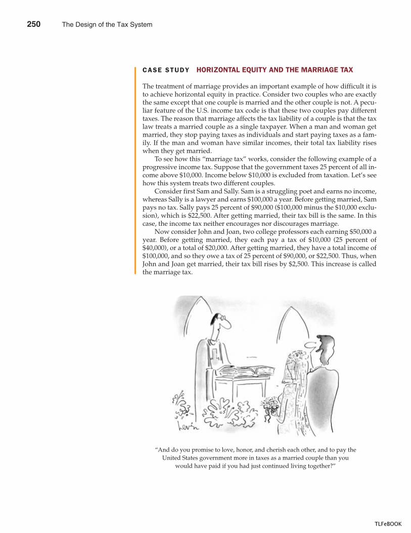
258 PART FOUR THE ECONOMICS OF THE PUBLIC SECTOR
CASE STUDY HORIZONTAL EQUITY AND THE MARRIAGE TAX
The treatment of marriage provides an important example of how difficult it isto achieve horizontal equity in practice. Consider two couples who are exactlythe same except that one couple is married and the other couple is not. A pecu-liar feature of the U.S. income tax code is that these two couples pay differenttaxes. The reason that marriage affects the tax liability of a couple is that the taxlaw treats a married couple as a single taxpayer. When a man and woman getmarried, they stop paying taxes as individuals and start paying taxes as a fam-ily. If the man and woman have similar incomes, their total tax liability riseswhen they get married.
To see how this “marriage tax” works, consider the following example of aprogressive income tax. Suppose that the government taxes 25 percent of all in-come above $10,000. Income below $10,000 is excluded from taxation. Let’s seehow this system treats two different couples.
Consider first Sam and Sally. Sam is a struggling poet and earns no income,whereas Sally is a lawyer and earns $100,000 a year. Before getting married, Sampays no tax. Sally pays 25 percent of $90,000 ($100,000 minus the $10,000 exclu-sion), which is $22,500. After getting married, their tax bill is the same. In thiscase, the income tax neither encourages nor discourages marriage.
Now consider John and Joan, two college professors each earning $50,000 ayear. Before getting married, they each pay a tax of $10,000 (25 percent of$40,000), or a total of $20,000. After getting married, they have a total income of$100,000, and so they owe a tax of 25 percent of $90,000, or $22,500. Thus, whenJohn and Joan get married, their tax bill rises by $2,500. This increase is calledthe marriage tax.
“And do you promise to love, honor, and cherish each other, and to pay theUnited States government more in taxes as a married couple than you
would have paid if you had just continued living together?”
250 The Design of the Tax System
TLFeBOOK
CHAPTER 12 THE DESIGN OF THE TAX SYSTEM 259
We can fix the problem for John and Joan by raising the income exclusionfrom $10,000 to $20,000 for married couples. But this change would create an-other problem. In this case, Sam and Sally would pay a tax after getting marriedof only $20,000, which is $2,500 less than they paid when they were single. Elim-inating the marriage tax for John and Joan would create a marriage subsidy forSam and Sally.
In practice, the U.S. tax code is an uneasy compromise that includes a com-bination of marriage taxes and marriage subsidies. According to a study by theCongressional Budget Office, 42 percent of married couples pay a marriage tax,averaging 2.0 percent of their income, while 51 percent of married couples paylower taxes by virtue of being wed, averaging 2.3 percent of their income.Whether a couple is better off (from a tax standpoint) being married or shackedup depends on how earnings are split between the two partners. If a man andwoman have similar incomes (like John and Joan), their wedding will mostlikely raise their tax bill. But a marriage subsidy is likely if one partner earnsmuch more than the other, and especially if only one of them has earnings (likeSam and Sally).
This problem has no simple solution. To see why, try designing an incometax with the following four properties:
� Two married couples with the same total income should pay the same tax.� When two people get married, their total tax bill should not change.� A person or family with no income should pay no taxes.� High-income taxpayers should pay a higher fraction of their incomes than
low-income taxpayers.
All four of these properties are appealing, yet it is impossible to satisfy all ofthem simultaneously. Any income tax that satisfies the first three must violatethe fourth. The only income tax that satisfies the first three properties is a pro-portional tax.
Some economists have advocated abolishing the marriage penalty by mak-ing individuals rather than the family the taxpaying unit, a policy that manyEuropean countries follow. This alternative might seem more equitable becauseit would treat married and unmarried couples the same. Yet this change wouldgive up on the first of these properties: Families with the same total incomecould end up paying different taxes. For example, if each married couple paidtaxes as if they were not married, then Sam and Sally would pay $22,500, andJohn and Joan would pay $20,000, even though both couples have the same to-tal income. Whether this alternative tax system is more or less fair than the cur-rent marriage tax is hard to say.
TAX INCIDENCE AND TAX EQUITY
Tax incidence—the study of who bears the burden of taxes—is central to evaluat-ing tax equity. As we first saw in Chapter 6, the person who bears the burden of atax is not always the person who gets the tax bill from the government. Becausetaxes alter supply and demand, they alter equilibrium prices. As a result, theyaffect people beyond those who, according to statute, actually pay the tax. When
The Design of the Tax System 251
TLFeBOOK
260 PART FOUR THE ECONOMICS OF THE PUBLIC SECTOR
CASE STUDY WHO PAYS THE CORPORATE INCOME TAX?
The corporate income tax provides a good example of the importance of tax in-cidence for tax policy. The corporate tax is popular among voters. After all, cor-porations are not people. Voters are always eager to have their taxes reducedand have some impersonal corporation pick up the tab.
But before deciding that the corporate income tax is a good way for the gov-ernment to raise revenue, we should consider who bears the burden of the cor-porate tax. This is a difficult question on which economists disagree, but onething is certain: People pay all taxes. When the government levies a tax on a cor-poration, the corporation is more like a tax collector than a taxpayer. The bur-den of the tax ultimately falls on people—the owners, customers, or workers ofthe corporation.
Many economists believe that workers and customers bear much of theburden of the corporate income tax. To see why, consider an example. Supposethat the U.S. government decides to raise the tax on the income earned by carcompanies. At first, this tax hurts the owners of the car companies, who receiveless profit. But, over time, these owners will respond to the tax. Because pro-ducing cars is less profitable, they invest less in building new car factories. In-stead, they invest their wealth in other ways—for example, by buying largerhouses or by building factories in other industries or other countries. Withfewer car factories, the supply of cars declines, as does the demand for auto-workers. Thus, a tax on corporations making cars causes the price of cars to riseand the wages of autoworkers to fall.
The corporate income tax shows how dangerous the flypaper theory of taxincidence can be. The corporate income tax is popular in part because it appearsto be paid by rich corporations. Yet those who bear the ultimate burden of thetax—the customers and workers of corporations—are often not rich. If the trueincidence of the corporate tax were more widely known, this tax might be lesspopular among voters.
CASE STUDY THE FLAT TAX
A recurring topic of debate is whether the U.S. federal government should com-pletely scrap the current tax system and replace it with a much simpler system
evaluating the vertical and horizontal equity of any tax, it is important to take ac-count of these indirect effects.
Many discussions of tax equity ignore the indirect effects of taxes and arebased on what economists mockingly call the flypaper theory of tax incidence. Ac-cording to this theory, the burden of a tax, like a fly on flypaper, sticks wherever itfirst lands. This assumption, however, is rarely valid.
For example, a person not trained in economics might argue that a tax on ex-pensive fur coats is vertically equitable because most buyers of furs are wealthy.Yet if these buyers can easily substitute other luxuries for furs, then a tax on fursmight only reduce the sale of furs. In the end, the burden of the tax will fall moreon those who make and sell furs than on those who buy them. Because most work-ers who make furs are not wealthy, the equity of a fur tax could be quite differentfrom what the flypaper theory indicates.
THIS WORKER PAYS PART OF THE
CORPORATE INCOME TAX.
252 The Design of the Tax System
TLFeBOOK
CHAPTER 12 THE DESIGN OF THE TAX SYSTEM 261
called the flat tax. The flat tax was proposed in the early 1980s by economistRobert Hall and political scientist Alvin Rabushka. Since then, it has from timeto time caught the attention of politicians on both the political left (such as JerryBrown, former governor of California and sometime candidate in the Demo-cratic presidential primaries) and the political right (such as Steve Forbes, multi-millionaire publisher and sometime candidate in the Republican presidentialprimaries).
Although flat-tax advocates have proposed various plans that differ in de-tail, the essence of all the plans is a single, low tax rate that would apply to allincome in the economy. If the tax rate were set at 19 percent, for example, thenevery taxpayer in the economy would face a marginal tax rate of 19 percent.Most of the plans allow a certain amount of income to be excluded from thetax. If the income exclusion were $10,000, for instance, then a person’s tax billwould be
Tax � 0.19 � (Income � $10,000).
Because of the income exclusion, a flat tax can be progressive: Average tax ratesrise with income, even though the marginal tax rate is constant. Some of theplans even allow a person with very low income (in this example, less than$10,000) to pay a “negative tax” by receiving a check from the government.
Because the flat-tax proposal calls for a major overhaul of the tax system,it raises almost every issue discussed in this chapter, especially the tradeoffbetween efficiency and equity. Here are some of the points made by flat-taxadvocates:
� The flat tax would eliminate many of the deductions allowed under thecurrent income tax, such as deductions for mortgage interest paymentsand charitable giving. By broadening the tax base in this way, the flat tax isable to reduce the marginal tax rates that most people face. Lower taxrates mean greater economic efficiency. Thus, flat-tax advocates claim thatthis change would expand the size of the economic pie.
� Because the flat tax is so simple, the administrative burden of taxationwould be greatly reduced. Flat-tax advocates claim that many taxpayerscould file their returns on a postcard. Because all taxpayers would paythe same low tax rate on all forms of income, people would have lessincentive to hire tax lawyers and accountants to take advantage ofloopholes.
� Because all taxpayers would face the same marginal tax rate, the taxcould be collected at the source of income rather than from the personwho receives the income. Income from corporate profit, for instance,would be taxed at the corporate level rather than at the personal level.This additional simplification also reduces administrative costs.
� The flat tax would replace both the personal income tax and the corporateincome tax. All income, whether from working at a job or from owningshares in a corporation, would be taxed once at the same marginal rate.The flat tax would eliminate the current double taxation of corporateprofits, which now discourages corporations from investing in new plantsand equipment.
The Design of the Tax System 253
TLFeBOOK
262 PART FOUR THE ECONOMICS OF THE PUBLIC SECTOR
� In computing income for tax purposes, businesses would be allowed todeduct all legitimate business expenses, including expenses on newinvestment goods. This deduction for investment makes the flat tax morelike a consumption tax than an income tax. As a result, a change to a flattax would increase the incentive to save (or, more precisely, wouldeliminate the current tax system’s disincentive to save).
In short, advocates of the flat tax claim that there is a strong efficiency argumentfor this dramatic tax reform.
Critics of the flat tax are sympathetic with the goal of a simpler and more ef-ficient tax system, but they oppose the flat tax because they believe that it givestoo little weight to the goal of vertical equity. They claim that a flat tax would beless progressive than the current tax system and, in particular, would shift someof the tax burden from the wealthy to the middle class. This concern may wellbe justified, but no one knows for sure. Our study of tax incidence shows thatthe burden of a tax is not necessarily borne by the person who sends the checkto the government. If the flat tax did encourage greater saving, as advocatesclaim, it would lead to more rapid economic growth, which would benefit alltaxpayers. No one can be certain, however, about how large the impact on eco-nomic growth would be.
QUICK QUIZ: Explain the benefits principle and the ability-to-pay principle.� What are vertical equity and horizontal equity? � Why is studying tax incidence important for determining the equity of a tax system?
CONCLUSION: THE TRADEOFF BETWEENEQUITY AND EFFICIENCY
Almost everyone agrees that equity and efficiency are the two most importantgoals of the tax system. But often these two goals conflict. Many proposed changesin the tax laws increase efficiency while reducing equity, or increase equity whilereducing efficiency. People disagree about tax policy often because they attach dif-ferent weights to these two goals.
The recent history of tax policy shows how political leaders differ in theirviews on equity and efficiency. When Ronald Reagan was elected president in1980, the marginal tax rate on the earnings of the richest Americans was 50 per-cent. On interest income, the marginal tax rate was 70 percent. Reagan argued thatsuch high tax rates greatly distorted economic incentives to work and save. Inother words, he claimed that these high tax rates cost too much in terms of eco-nomic efficiency. Tax reform was, therefore, a high priority of his administration.Reagan signed into law large cuts in tax rates in 1981 and then again in 1986. WhenReagan left office in 1989, the richest Americans faced a marginal tax rate of only28 percent. During the four years of the Bush presidency, the top tax rate increasedslightly to 31 percent.
When Bill Clinton ran for president in 1992, he argued that the rich werenot paying their fair share of taxes. In other words, the low tax rates on the rich
254 The Design of the Tax System
TLFeBOOK
CHAPTER 12 THE DESIGN OF THE TAX SYSTEM 263
violated his view of vertical equity. One of President Clinton’s first acts was to pro-pose raising the tax rates on the highest levels of income. In 1993 the tax rates onthe richest Americans became about 40 percent.
Economics alone cannot determine the best way to balance the goals of effi-ciency and equity. This issue involves political philosophy as well as economics.But economists do have an important role in the political debate over tax policy:They can shed light on the tradeoffs that society faces and can help us avoid poli-cies that sacrifice efficiency without any benefit in terms of equity.
� The U.S. government raises revenue using various taxes.The most important taxes for the federal governmentare individual income taxes and payroll taxes for socialinsurance. The most important taxes for state and localgovernments are sales taxes and property taxes.
� The efficiency of a tax system refers to the costs itimposes on taxpayers. There are two costs of taxesbeyond the transfer of resources from the taxpayer tothe government. The first is the distortion in theallocation of resources that arises as taxes alterincentives and behavior. The second is theadministrative burden of complying with the tax laws.
� The equity of a tax system concerns whether the taxburden is distributed fairly among the population.
According to the benefits principle, it is fair for peopleto pay taxes based on the benefits they receive from thegovernment. According to the ability-to-pay principle, itis fair for people to pay taxes based on their capabilityto handle the financial burden. When evaluating theequity of a tax system, it is important to remember alesson from the study of tax incidence: The distributionof tax burdens is not the same as the distribution oftax bills.
� When considering changes in the tax laws,policymakers often face a tradeoff between efficiencyand equity. Much of the debate over tax policy arisesbecause people give different weights to these twogoals.
Summar y
budget surplus, p. 248budget deficit, p. 248average tax rate, p. 252marginal tax rate, p. 252
lump-sum tax, p. 254benefits principle, p. 255ability-to-pay principle, p. 255vertical equity, p. 256
horizontal equity, p. 256proportional tax, p. 256regressive tax, p. 256progressive tax, p. 256
Key Concepts
1. Over the past several decades, has government grownmore or less slowly than the rest of the economy?
2. What are the two most important sources of revenue forthe U.S. federal government?
3. Explain how corporate profits are taxed twice.
4. Why is the burden of a tax to taxpayers greater than therevenue received by the government?
5. Why do some economists advocate taxing consumptionrather than income?
6. Give two arguments why wealthy taxpayers should paymore taxes than poor taxpayers.
7. What is the concept of horizontal equity, and why is ithard to apply?
8. Describe the arguments for and against replacing thecurrent tax system with a flat tax.
Quest ions fo r Rev iew
The Design of the Tax System 255
TLFeBOOK
264 PART FOUR THE ECONOMICS OF THE PUBLIC SECTOR
1. Government spending in the United States has grown asa share of national income over time. What changes inour economy and our society might explain this trend?Do you expect the trend to continue?
2. In a published source or on the Internet, find outwhether the U.S. federal government had a budgetdeficit or surplus last year. What do policymakersexpect to happen over the next few years? (Hint: TheWeb site of the Congressional Budget Office iswww.cbo.gov.)
3. The information in many of the tables in this chapteris taken from the Economic Report of the President,which appears annually. Using a recent issue ofthe report at your library, answer the followingquestions and provide some numbers to supportyour answers.a. Figure 12-1 shows that government revenue as a
percentage of total income has increased over time.Is this increase primarily attributable to changes infederal government revenue or in state and localgovernment revenue?
b. Looking at the combined revenue of the federalgovernment and state and local governments, howhas the composition of total revenue changed overtime? Are personal income taxes more or lessimportant? Social insurance taxes? Corporateprofits taxes?
c. Looking at the combined expenditures of thefederal government and state and localgovernments, how have the relative shares oftransfer payments and purchases of goods andservices changed over time?
4. The chapter states that the elderly population in theUnited States is growing more rapidly than the totalpopulation. In particular, the number of workers isrising slowly, while the number of retirees is risingquickly. Concerned about the future of Social Security,some members of Congress propose a “freeze” on theprogram.a. If total expenditures were frozen, what would
happen to benefits per retiree? To tax payments perworker? (Assume that Social Security taxes andreceipts are balanced in each year.)
b. If benefits per retiree were frozen, what wouldhappen to total expenditures? To tax payments perworker?
c. If tax payments per worker were frozen, whatwould happen to total expenditures? To benefitsper retiree?
d. What do your answers to parts (a), (b), and (c)imply about the difficult decisions faced bypolicymakers?
5. Suppose you are a typical person in the U.S. economy.You pay a flat 4 percent of your income in a state incometax and 15.3 percent of your labor earnings in federalpayroll taxes (employer and employee sharescombined). You also pay federal income taxes as inTable 12-3. How much tax of each type do you pay ifyou earn $20,000 a year? Taking all taxes into account,what are your average and marginal tax rates? Whathappens to your tax bill and to your average andmarginal tax rates if your income rises to $40,000?
6. Some states exclude necessities, such as food andclothing, from their sales tax. Other states do not.Discuss the merits of this exclusion. Consider bothefficiency and equity.
7. Explain how individuals’ behavior is affected by thefollowing features of the federal tax code.a. Contributions to charity are tax deductible.b. Sales of beer are taxed.c. Interest that a homeowner pays on a mortgage is
tax deductible.d. Realized capital gains are taxed, but accrued gains
are not. (When someone owns a share of stock thatrises in value, she has an “accrued” capital gain. Ifshe sells the share, she has a “realized” gain.)
8. Suppose that your state raises its sales tax from5 percent to 6 percent. The state revenue commissionerforecasts a 20 percent increase in sales tax revenue. Isthis plausible? Explain.
9. Consider two of the income security programs in theUnited States: Temporary Assistance for Needy Families(TANF) and the Earned Income Tax Credit (EITC).a. When a woman with children and very low income
earns an extra dollar, she receives less in TANFbenefits. What do you think is the effect of thisfeature of TANF on the labor supply of low-incomewomen? Explain.
b. The EITC provides greater benefits as low-incomeworkers earn more income (up to a point). What doyou think is the effect of this program on the laborsupply of low-income individuals? Explain.
Prob lems and App l icat ions
256 The Design of the Tax System
TLFeBOOK
CHAPTER 12 THE DESIGN OF THE TAX SYSTEM 265
c. What are the disadvantages of eliminating TANFand allocating the savings to the EITC?
10. The Tax Reform Act of 1986 eliminated the deductibilityof interest payments on consumer debt (mostly creditcards and auto loans) but maintained the deductibilityof interest payments on mortgages and home equityloans. What do you think happened to the relativeamounts of borrowing through consumer debt andhome equity debt?
11. Categorize each of the following funding schemes asexamples of the benefits principle or the ability-to-payprinciple.a. Visitors to many national parks pay an entrance fee.b. Local property taxes support elementary and
secondary schools.c. An airport trust fund collects a tax on each plane
ticket sold and uses the money to improve airportsand the air traffic control system.
12. Any income tax schedule embodies two types of taxrates—average tax rates and marginal tax rates.a. The average tax rate is defined as total taxes paid
divided by income. For the proportional tax systempresented in Table 12-7, what are the average taxrates for people earning $50,000, $100,000, and$200,000? What are the corresponding average taxrates in the regressive and progressive tax systems?
b. The marginal tax rate is defined as the extra taxespaid on additional income divided by the increase
in income. Calculate the marginal tax rate for theproportional tax system as income rises from$50,000 to $100,000. Calculate the marginal tax rateas income rises from $100,000 to $200,000. Calculatethe corresponding marginal tax rates for theregressive and progressive tax systems.
c. Describe the relationship between average tax ratesand marginal tax rates for each of these threesystems. In general, which rate is relevant forsomeone deciding whether to accept a job that paysslightly more than her current job? Which rate isrelevant for judging the vertical equity of a taxsystem?
13. What is the efficiency justification for taxingconsumption rather than income? If the United Stateswere to adopt a consumption tax, do you think thatwould make the U.S. tax system more or lessprogressive? Explain.
14. If a salesman takes a client to lunch, part of the cost ofthe lunch is a deductible business expense for hiscompany. Some members of Congress have argued thatthis feature of the tax code benefits relatively wealthybusinesspeople and should be eliminated. Yet theirarguments have been met with greater opposition fromeating and drinking establishments than fromcompanies themselves. Explain.
The Design of the Tax System 257
TLFeBOOK

TLFeBOOK
IN THIS CHAPTERYOU WILL . . .
Examine there lat ionsh ip
between shor t - r unand long - r un costs
Learn the meaningof average tota l
cost and marg ina lcost and how they
are r e lated
Examine what i temsare inc luded in a
f i rm’s costs o fproduct ion
Analyze the l inkbetween a f i rm’s
product ion processand i ts tota l costs
Cons ider the shapeof a typ ica l f i rm’s
cost cur ves
The economy is made up of thousands of firms that produce the goods and ser-vices you enjoy every day: General Motors produces automobiles, General Electricproduces lightbulbs, and General Mills produces breakfast cereals. Some firms,such as these three, are large; they employ thousands of workers and have thou-sands of stockholders who share in the firms’ profits. Other firms, such as the localbarbershop or candy store, are small; they employ only a few workers and areowned by a single person or family.
In previous chapters we used the supply curve to summarize firms’ produc-tion decisions. According to the law of supply, firms are willing to produce and sella greater quantity of a good when the price of the good is higher, and this responseleads to a supply curve that slopes upward. For analyzing many questions, the lawof supply is all you need to know about firm behavior.
In this chapter and the ones that follow, we examine firm behavior in more de-tail. This topic will give you a better understanding of what decisions lie behind
T H E C O S T S O F P R O D U C T I O N
269
259
13
TLFeBOOK
270 PART F IVE FIRM BEHAVIOR AND THE ORGANIZATION OF INDUSTRY
the supply curve in a market. In addition, it will introduce you to a part of eco-nomics called industrial organization—the study of how firms’ decisions regardingprices and quantities depend on the market conditions they face. The town inwhich you live, for instance, may have several pizzerias but only one cable televi-sion company. How does this difference in the number of firms affect the prices inthese markets and the efficiency of the market outcomes? The field of industrial or-ganization addresses exactly this question.
As a starting point for the study of industrial organization, this chapter exam-ines the costs of production. All firms, from Delta Air Lines to your local deli, in-cur costs as they make the goods and services that they sell. As we will see in thecoming chapters, a firm’s costs are a key determinant of its production and pricingdecisions. Establishing what a firm’s costs are, however, is not as straightforwardas it might seem.
WHAT ARE COSTS?
We begin our discussion of costs at Hungry Helen’s Cookie Factory. Helen, theowner of the firm, buys flour, sugar, flavorings, and other cookie ingredients. Shealso buys the mixers and ovens and hires workers to run this equipment. She thensells the resulting cookies to consumers. By examining some of the issues that He-len faces in her business, we can learn some lessons that apply to all firms in theeconomy.
TOTAL REVENUE, TOTAL COST, AND PROFIT
We begin with the firm’s objective. To understand what decisions a firm makes, wemust understand what it is trying to do. It is conceivable that Helen started herfirm because of an altruistic desire to provide the world with cookies or, perhaps,out of love for the cookie business. More likely, however, Helen started her busi-ness to make money. Economists normally assume that the goal of a firm is to max-imize profit, and they find that this assumption works well in most cases.
What is a firm’s profit? The amount that the firm receives for the sale of its out-put (cookies) is called its total revenue. The amount that the firm pays to buy in-puts (flour, sugar, workers, ovens, etc.) is called its total cost. Helen gets to keepany revenue that is not needed to cover costs. We define profit as a firm’s total rev-enue minus its total cost. That is,
Profit � Total revenue � Total cost.
Helen’s objective is to make her firm’s profit as large as possible.To see how a firm goes about maximizing profit, we must consider fully how
to measure its total revenue and its total cost. Total revenue is the easy part: Itequals the quantity of output the firm produces times the price at which it sells itsoutput. If Helen produces 10,000 cookies and sells them at $2 a cookie, her totalrevenue is $20,000. By contrast, the measurement of a firm’s total cost is moresubtle.
tota l r evenuethe amount a firm receives for thesale of its output
tota l costthe market value of the inputs a firmuses in production
pro f i ttotal revenue minus total cost
260 The Costs of Production
TLFeBOOK
CHAPTER 13 THE COSTS OF PRODUCTION 271
COSTS AS OPPORTUNITY COSTS
When measuring costs at Hungry Helen’s Cookie Factory or any other firm, it isimportant to keep in mind one of the Ten Principles of Economics from Chapter 1:The cost of something is what you give up to get it. Recall that the opportunity costof an item refers to all those things that must be forgone to acquire that item. Wheneconomists speak of a firm’s cost of production, they include all the opportunitycosts of making its output of goods and services.
A firm’s opportunity costs of production are sometimes obvious and sometimesless so. When Helen pays $1,000 for flour, that $1,000 is an opportunity cost becauseHelen can no longer use that $1,000 to buy something else. Similarly, when Helenhires workers to make the cookies, the wages she pays are part of the firm’s costs.These are explicit costs. By contrast, some of a firm’s opportunity costs are implicitcosts. Imagine that Helen is skilled with computers and could earn $100 per hourworking as a programmer. For every hour that Helen works at her cookie factory,she gives up $100 in income, and this forgone income is also part of her costs.
This distinction between explicit and implicit costs highlights an importantdifference between how economists and accountants analyze a business. Econo-mists are interested in studying how firms make production and pricing decisions.Because these decisions are based on both explicit and implicit costs, economistsinclude both when measuring a firm’s costs. By contrast, accountants have the jobof keeping track of the money that flows into and out of firms. As a result, theymeasure the explicit costs but often ignore the implicit costs.
The difference between economists and accountants is easy to see in the caseof Hungry Helen’s Cookie Factory. When Helen gives up the opportunity to earnmoney as a computer programmer, her accountant will not count this as a cost ofher cookie business. Because no money flows out of the business to pay for thiscost, it never shows up on the accountant’s financial statements. An economist,however, will count the forgone income as a cost because it will affect the decisionsthat Helen makes in her cookie business. For example, if Helen’s wage as a com-puter programmer rises from $100 to $500 per hour, she might decide that runningher cookie business is too costly and choose to shut down the factory in order tobecome a full-time computer programmer.
THE COST OF CAPITAL AS AN OPPORTUNITY COST
An important implicit cost of almost every business is the opportunity cost of the fi-nancial capital that has been invested in the business. Suppose, for instance, that He-len used $300,000 of her savings to buy her cookie factory from the previous owner.If Helen had instead left this money deposited in a savings account that pays an in-terest rate of 5 percent, she would have earned $15,000 per year. To own her cookiefactory, therefore, Helen has given up $15,000 a year in interest income. This forgone$15,000 is one of the implicit opportunity costs of Helen’s business.
As we have already noted, economists and accountants treat costs differently,and this is especially true in their treatment of the cost of capital. An economistviews the $15,000 in interest income that Helen gives up every year as a cost of herbusiness, even though it is an implicit cost. Helen’s accountant, however, will notshow this $15,000 as a cost because no money flows out of the business to pay for it.
To further explore the difference between economists and accountants, let’schange the example slightly. Suppose now that Helen did not have the entire
expl ic i t costsinput costs that require an outlay ofmoney by the firm
impl ic i t costsinput costs that do not require anoutlay of money by the firm
The Costs of Production 261
TLFeBOOK
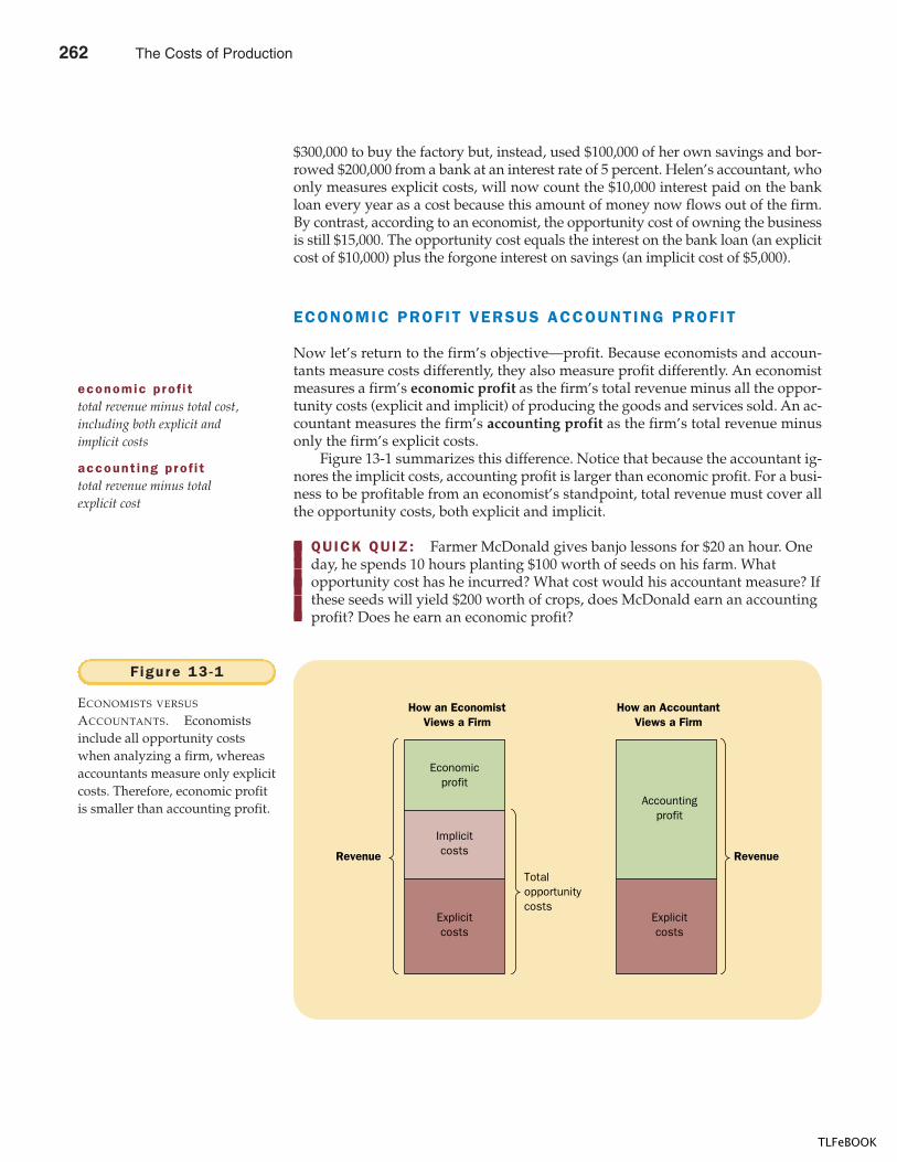
272 PART F IVE FIRM BEHAVIOR AND THE ORGANIZATION OF INDUSTRY
$300,000 to buy the factory but, instead, used $100,000 of her own savings and bor-rowed $200,000 from a bank at an interest rate of 5 percent. Helen’s accountant, whoonly measures explicit costs, will now count the $10,000 interest paid on the bankloan every year as a cost because this amount of money now flows out of the firm.By contrast, according to an economist, the opportunity cost of owning the businessis still $15,000. The opportunity cost equals the interest on the bank loan (an explicitcost of $10,000) plus the forgone interest on savings (an implicit cost of $5,000).
ECONOMIC PROFIT VERSUS ACCOUNTING PROFIT
Now let’s return to the firm’s objective—profit. Because economists and accoun-tants measure costs differently, they also measure profit differently. An economistmeasures a firm’s economic profit as the firm’s total revenue minus all the oppor-tunity costs (explicit and implicit) of producing the goods and services sold. An ac-countant measures the firm’s accounting profit as the firm’s total revenue minusonly the firm’s explicit costs.
Figure 13-1 summarizes this difference. Notice that because the accountant ig-nores the implicit costs, accounting profit is larger than economic profit. For a busi-ness to be profitable from an economist’s standpoint, total revenue must cover allthe opportunity costs, both explicit and implicit.
QUICK QUIZ: Farmer McDonald gives banjo lessons for $20 an hour. One day, he spends 10 hours planting $100 worth of seeds on his farm. What opportunity cost has he incurred? What cost would his accountant measure? Ifthese seeds will yield $200 worth of crops, does McDonald earn an accounting profit? Does he earn an economic profit?
economic pro f i ttotal revenue minus total cost,including both explicit andimplicit costs
account ing pro f i ttotal revenue minus totalexplicit cost
Revenue
Totalopportunitycosts
How an EconomistViews a Firm
Economicprofit
Implicitcosts
Explicitcosts
Explicitcosts
Accountingprofit
How an AccountantViews a Firm
Revenue
F igure 13 -1
ECONOMISTS VERSUS
ACCOUNTANTS. Economistsinclude all opportunity costswhen analyzing a firm, whereasaccountants measure only explicitcosts. Therefore, economic profitis smaller than accounting profit.
262 The Costs of Production
TLFeBOOK
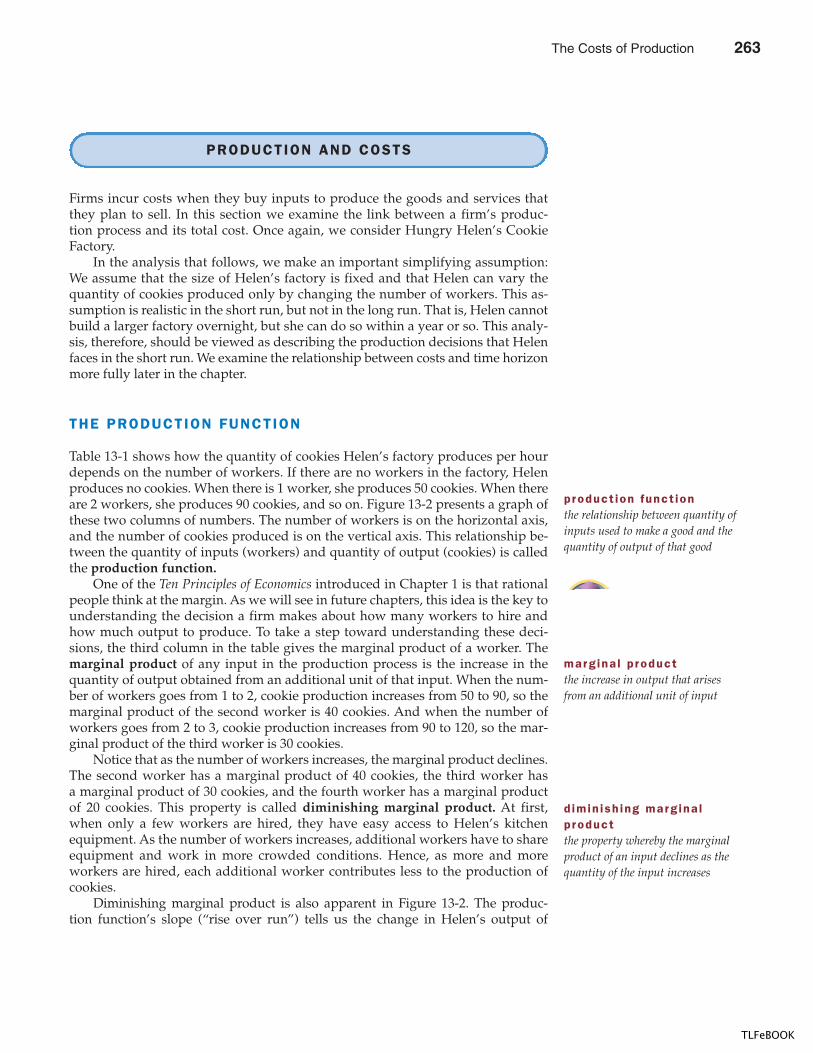
CHAPTER 13 THE COSTS OF PRODUCTION 273
PRODUCTION AND COSTS
Firms incur costs when they buy inputs to produce the goods and services thatthey plan to sell. In this section we examine the link between a firm’s produc-tion process and its total cost. Once again, we consider Hungry Helen’s CookieFactory.
In the analysis that follows, we make an important simplifying assumption:We assume that the size of Helen’s factory is fixed and that Helen can vary thequantity of cookies produced only by changing the number of workers. This as-sumption is realistic in the short run, but not in the long run. That is, Helen cannotbuild a larger factory overnight, but she can do so within a year or so. This analy-sis, therefore, should be viewed as describing the production decisions that Helenfaces in the short run. We examine the relationship between costs and time horizonmore fully later in the chapter.
THE PRODUCTION FUNCTION
Table 13-1 shows how the quantity of cookies Helen’s factory produces per hourdepends on the number of workers. If there are no workers in the factory, Helenproduces no cookies. When there is 1 worker, she produces 50 cookies. When thereare 2 workers, she produces 90 cookies, and so on. Figure 13-2 presents a graph ofthese two columns of numbers. The number of workers is on the horizontal axis,and the number of cookies produced is on the vertical axis. This relationship be-tween the quantity of inputs (workers) and quantity of output (cookies) is calledthe production function.
One of the Ten Principles of Economics introduced in Chapter 1 is that rationalpeople think at the margin. As we will see in future chapters, this idea is the key tounderstanding the decision a firm makes about how many workers to hire andhow much output to produce. To take a step toward understanding these deci-sions, the third column in the table gives the marginal product of a worker. Themarginal product of any input in the production process is the increase in thequantity of output obtained from an additional unit of that input. When the num-ber of workers goes from 1 to 2, cookie production increases from 50 to 90, so themarginal product of the second worker is 40 cookies. And when the number ofworkers goes from 2 to 3, cookie production increases from 90 to 120, so the mar-ginal product of the third worker is 30 cookies.
Notice that as the number of workers increases, the marginal product declines.The second worker has a marginal product of 40 cookies, the third worker hasa marginal product of 30 cookies, and the fourth worker has a marginal productof 20 cookies. This property is called diminishing marginal product. At first,when only a few workers are hired, they have easy access to Helen’s kitchenequipment. As the number of workers increases, additional workers have to shareequipment and work in more crowded conditions. Hence, as more and moreworkers are hired, each additional worker contributes less to the production ofcookies.
Diminishing marginal product is also apparent in Figure 13-2. The produc-tion function’s slope (“rise over run”) tells us the change in Helen’s output of
product ion funct ionthe relationship between quantity ofinputs used to make a good and thequantity of output of that good
marg ina l p roductthe increase in output that arisesfrom an additional unit of input
d imin ish ing marg ina lproductthe property whereby the marginalproduct of an input declines as thequantity of the input increases
The Costs of Production 263
TLFeBOOK
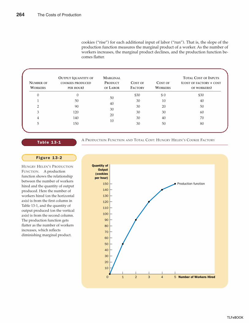
274 PART F IVE FIRM BEHAVIOR AND THE ORGANIZATION OF INDUSTRY
cookies (“rise”) for each additional input of labor (“run”). That is, the slope of theproduction function measures the marginal product of a worker. As the number ofworkers increases, the marginal product declines, and the production function be-comes flatter.
Quantity ofOutput
(cookiesper hour)
150
140
130
120
110
100
90
80
70
60
50
40
30
20
10
Number of Workers Hired0 1 2 3 4 5
Production function
Figure 13 -2
HUNGRY HELEN’S PRODUCTION
FUNCTION. A productionfunction shows the relationshipbetween the number of workershired and the quantity of outputproduced. Here the number ofworkers hired (on the horizontalaxis) is from the first column inTable 13-1, and the quantity ofoutput produced (on the verticalaxis) is from the second column.The production function getsflatter as the number of workersincreases, which reflectsdiminishing marginal product.
Table 13 -1
OUTPUT (QUANTITY OF MARGINAL TOTAL COST OF INPUTS
NUMBER OF COOKIES PRODUCED PRODUCT COST OF COST OF (COST OF FACTORY + COST
WORKERS PER HOUR) OF LABOR FACTORY WORKERS OF WORKERS)
0 0 $30 $ 0 $3050
1 50 30 10 4040
2 90 30 20 5030
3 120 30 30 6020
4 140 30 40 7010
5 150 30 50 80
A PRODUCTION FUNCTION AND TOTAL COST: HUNGRY HELEN’S COOKIE FACTORY
264 The Costs of Production
TLFeBOOK
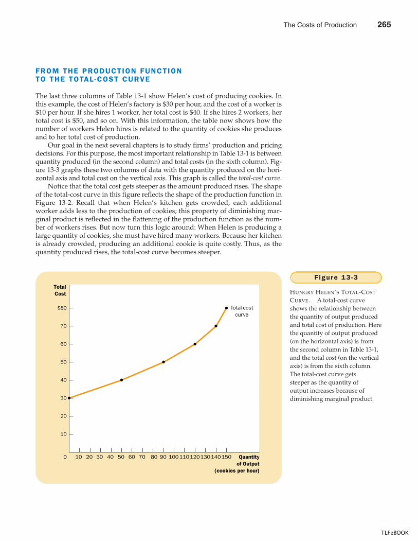
CHAPTER 13 THE COSTS OF PRODUCTION 275
FROM THE PRODUCTION FUNCTION TO THE TOTAL -COST CURVE
The last three columns of Table 13-1 show Helen’s cost of producing cookies. Inthis example, the cost of Helen’s factory is $30 per hour, and the cost of a worker is$10 per hour. If she hires 1 worker, her total cost is $40. If she hires 2 workers, hertotal cost is $50, and so on. With this information, the table now shows how thenumber of workers Helen hires is related to the quantity of cookies she producesand to her total cost of production.
Our goal in the next several chapters is to study firms’ production and pricingdecisions. For this purpose, the most important relationship in Table 13-1 is betweenquantity produced (in the second column) and total costs (in the sixth column). Fig-ure 13-3 graphs these two columns of data with the quantity produced on the hori-zontal axis and total cost on the vertical axis. This graph is called the total-cost curve.
Notice that the total cost gets steeper as the amount produced rises. The shapeof the total-cost curve in this figure reflects the shape of the production function inFigure 13-2. Recall that when Helen’s kitchen gets crowded, each additionalworker adds less to the production of cookies; this property of diminishing mar-ginal product is reflected in the flattening of the production function as the num-ber of workers rises. But now turn this logic around: When Helen is producing alarge quantity of cookies, she must have hired many workers. Because her kitchenis already crowded, producing an additional cookie is quite costly. Thus, as thequantity produced rises, the total-cost curve becomes steeper.
TotalCost
$80
70
60
50
40
30
20
10
Quantityof Output
(cookies per hour)
0 10 20 30 15013011090705040 1401201008060
Total-costcurve
Figure 13 -3
HUNGRY HELEN’S TOTAL-COST
CURVE. A total-cost curveshows the relationship betweenthe quantity of output producedand total cost of production. Herethe quantity of output produced(on the horizontal axis) is fromthe second column in Table 13-1,and the total cost (on the verticalaxis) is from the sixth column.The total-cost curve getssteeper as the quantity ofoutput increases because ofdiminishing marginal product.
The Costs of Production 265
TLFeBOOK
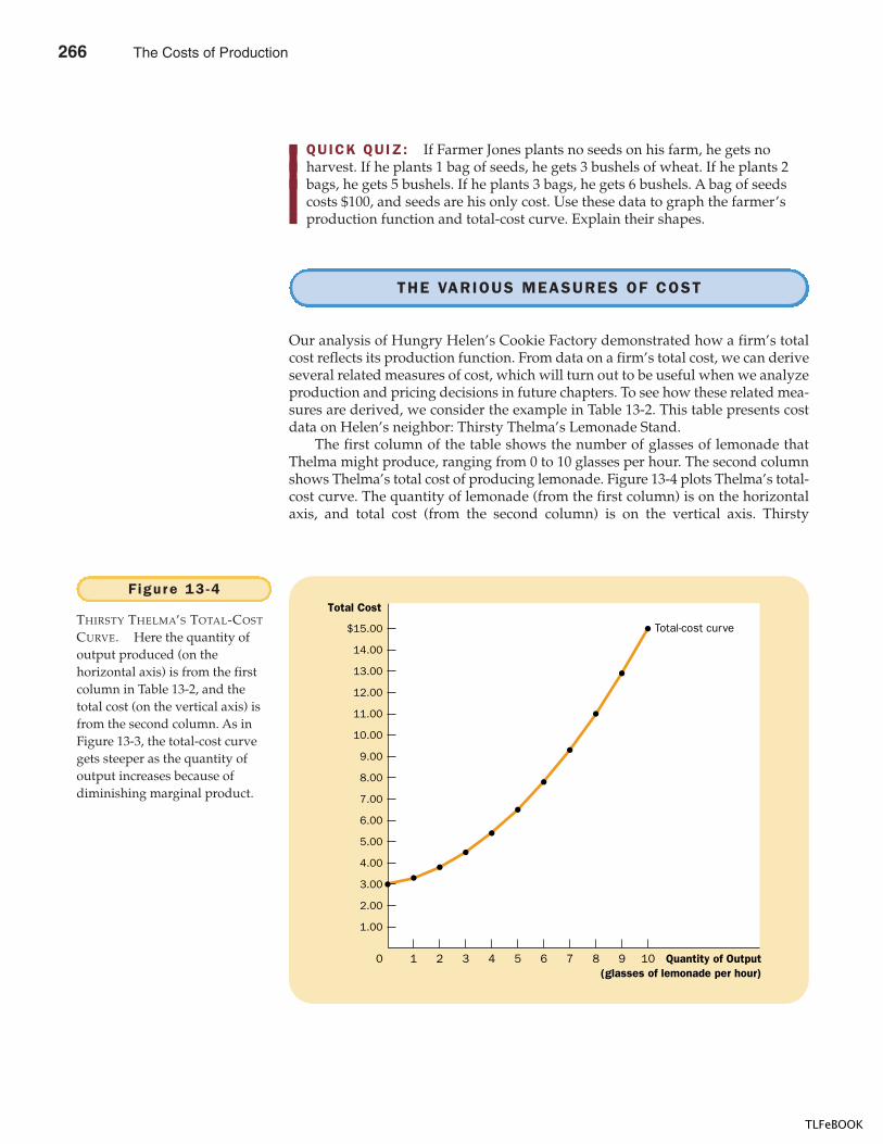
276 PART F IVE FIRM BEHAVIOR AND THE ORGANIZATION OF INDUSTRY
QUICK QUIZ: If Farmer Jones plants no seeds on his farm, he gets no harvest. If he plants 1 bag of seeds, he gets 3 bushels of wheat. If he plants 2 bags, he gets 5 bushels. If he plants 3 bags, he gets 6 bushels. A bag of seedscosts $100, and seeds are his only cost. Use these data to graph the farmer’s production function and total-cost curve. Explain their shapes.
THE VARIOUS MEASURES OF COST
Our analysis of Hungry Helen’s Cookie Factory demonstrated how a firm’s totalcost reflects its production function. From data on a firm’s total cost, we can deriveseveral related measures of cost, which will turn out to be useful when we analyzeproduction and pricing decisions in future chapters. To see how these related mea-sures are derived, we consider the example in Table 13-2. This table presents costdata on Helen’s neighbor: Thirsty Thelma’s Lemonade Stand.
The first column of the table shows the number of glasses of lemonade thatThelma might produce, ranging from 0 to 10 glasses per hour. The second columnshows Thelma’s total cost of producing lemonade. Figure 13-4 plots Thelma’s total-cost curve. The quantity of lemonade (from the first column) is on the horizontalaxis, and total cost (from the second column) is on the vertical axis. Thirsty
Total Cost
$15.00
14.00
13.00
12.00
11.00
10.00
9.00
8.00
7.00
6.00
5.00
4.00
3.00
2.00
1.00
Quantity of Output(glasses of lemonade per hour)
0 1 432 765 98 10
Total-cost curve
Figure 13 -4
THIRSTY THELMA’S TOTAL-COST
CURVE. Here the quantity ofoutput produced (on thehorizontal axis) is from the firstcolumn in Table 13-2, and thetotal cost (on the vertical axis) isfrom the second column. As inFigure 13-3, the total-cost curvegets steeper as the quantity ofoutput increases because ofdiminishing marginal product.
266 The Costs of Production
TLFeBOOK
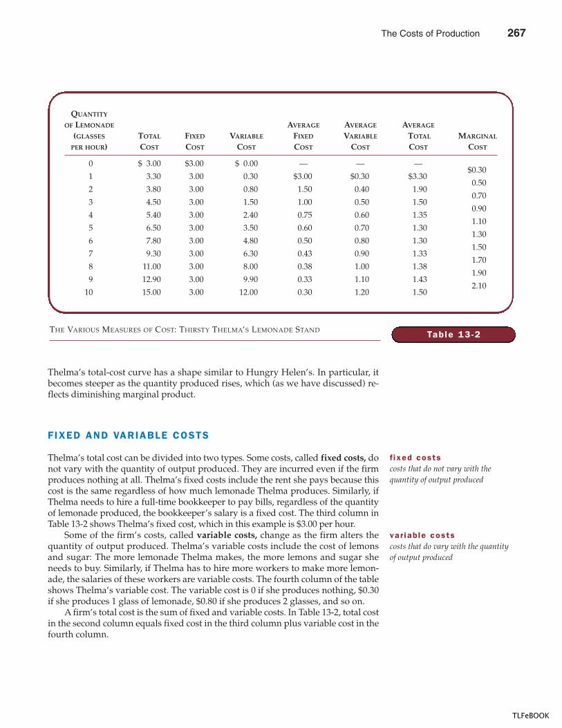
CHAPTER 13 THE COSTS OF PRODUCTION 277
Thelma’s total-cost curve has a shape similar to Hungry Helen’s. In particular, itbecomes steeper as the quantity produced rises, which (as we have discussed) re-flects diminishing marginal product.
FIXED AND VARIABLE COSTS
Thelma’s total cost can be divided into two types. Some costs, called fixed costs, donot vary with the quantity of output produced. They are incurred even if the firmproduces nothing at all. Thelma’s fixed costs include the rent she pays because thiscost is the same regardless of how much lemonade Thelma produces. Similarly, ifThelma needs to hire a full-time bookkeeper to pay bills, regardless of the quantityof lemonade produced, the bookkeeper’s salary is a fixed cost. The third column inTable 13-2 shows Thelma’s fixed cost, which in this example is $3.00 per hour.
Some of the firm’s costs, called variable costs, change as the firm alters thequantity of output produced. Thelma’s variable costs include the cost of lemonsand sugar: The more lemonade Thelma makes, the more lemons and sugar sheneeds to buy. Similarly, if Thelma has to hire more workers to make more lemon-ade, the salaries of these workers are variable costs. The fourth column of the tableshows Thelma’s variable cost. The variable cost is 0 if she produces nothing, $0.30if she produces 1 glass of lemonade, $0.80 if she produces 2 glasses, and so on.
A firm’s total cost is the sum of fixed and variable costs. In Table 13-2, total costin the second column equals fixed cost in the third column plus variable cost in thefourth column.
Table 13 -2
QUANTITY
OF LEMONADE AVERAGE AVERAGE AVERAGE
(GLASSES TOTAL FIXED VARIABLE FIXED VARIABLE TOTAL MARGINAL
PER HOUR) COST COST COST COST COST COST COST
0 $ 3.00 $3.00 $ 0.00 — — —$0.30
1 3.30 3.00 0.30 $3.00 $0.30 $3.300.50
2 3.80 3.00 0.80 1.50 0.40 1.900.70
3 4.50 3.00 1.50 1.00 0.50 1.500.90
4 5.40 3.00 2.40 0.75 0.60 1.351.10
5 6.50 3.00 3.50 0.60 0.70 1.301.30
6 7.80 3.00 4.80 0.50 0.80 1.301.50
7 9.30 3.00 6.30 0.43 0.90 1.331.70
8 11.00 3.00 8.00 0.38 1.00 1.381.90
9 12.90 3.00 9.90 0.33 1.10 1.432.10
10 15.00 3.00 12.00 0.30 1.20 1.50
THE VARIOUS MEASURES OF COST: THIRSTY THELMA’S LEMONADE STAND
f ixed costscosts that do not vary with thequantity of output produced
var iab le costscosts that do vary with the quantityof output produced
The Costs of Production 267
TLFeBOOK
278 PART F IVE FIRM BEHAVIOR AND THE ORGANIZATION OF INDUSTRY
AVERAGE AND MARGINAL COST
As the owner of her firm, Thelma has to decide how much to produce. A key partof this decision is how her costs will vary as she changes the level of production.In making this decision, Thelma might ask her production supervisor the follow-ing two questions about the cost of producing lemonade:
� How much does it cost to make the typical glass of lemonade?� How much does it cost to increase production of lemonade by 1 glass?
Although at first these two questions might seem to have the same answer, they donot. Both answers will turn out to be important for understanding how firms makeproduction decisions.
To find the cost of the typical unit produced, we would divide the firm’s costsby the quantity of output it produces. For example, if the firm produces 2 glassesper hour, its total cost is $3.80, and the cost of the typical glass is $3.80/2, or $1.90.Total cost divided by the quantity of output is called average total cost. Because to-tal cost is just the sum of fixed and variable costs, average total cost can be ex-pressed as the sum of average fixed cost and average variable cost. Average fixedcost is the fixed cost divided by the quantity of output, and average variable costis the variable cost divided by the quantity of output.
Although average total cost tells us the cost of the typical unit, it does not tellus how much total cost will change as the firm alters its level of production. Thelast column in Table 13-2 shows the amount that total cost rises when the firm in-creases production by 1 unit of output. This number is called marginal cost. Forexample, if Thelma increases production from 2 to 3 glasses, total cost rises from$3.80 to $4.50, so the marginal cost of the third glass of lemonade is $4.50 minus$3.80, or $0.70.
It may be helpful to express these definitions mathematically. If Q stands forquantity, TC for total cost, ATC for average total cost, and MC for marginal cost,then we can then write:
ATC = Total cost/Quantity = TC/Q
and
MC = (Change in total cost)/(Change in quantity) = �TC/�Q.
Here �, the Greek letter delta, represents the change in a variable. These equationsshow how average total cost and marginal cost are derived from total cost.
As we will see more fully in the next chapter, Thelma, our lemonade entrepre-neur, will find the concepts of average total cost and marginal cost extremely usefulwhen deciding how much lemonade to produce. Keep in mind, however, that theseconcepts do not actually give Thelma new information about her costs of production.Instead, average total cost and marginal cost express in a new way information thatis already contained in her firm’s total cost. Average total cost tells us the cost of a typicalunit of output if total cost is divided evenly over all the units produced. Marginal cost tells usthe increase in total cost that arises from producing an additional unit of output.
average tota l costtotal cost divided by the quantityof output
average f ixed costfixed costs divided by the quantityof output
average var iab le costvariable costs divided by the quantityof output
marg ina l costthe increase in total cost that arisesfrom an extra unit of production
268 The Costs of Production
TLFeBOOK
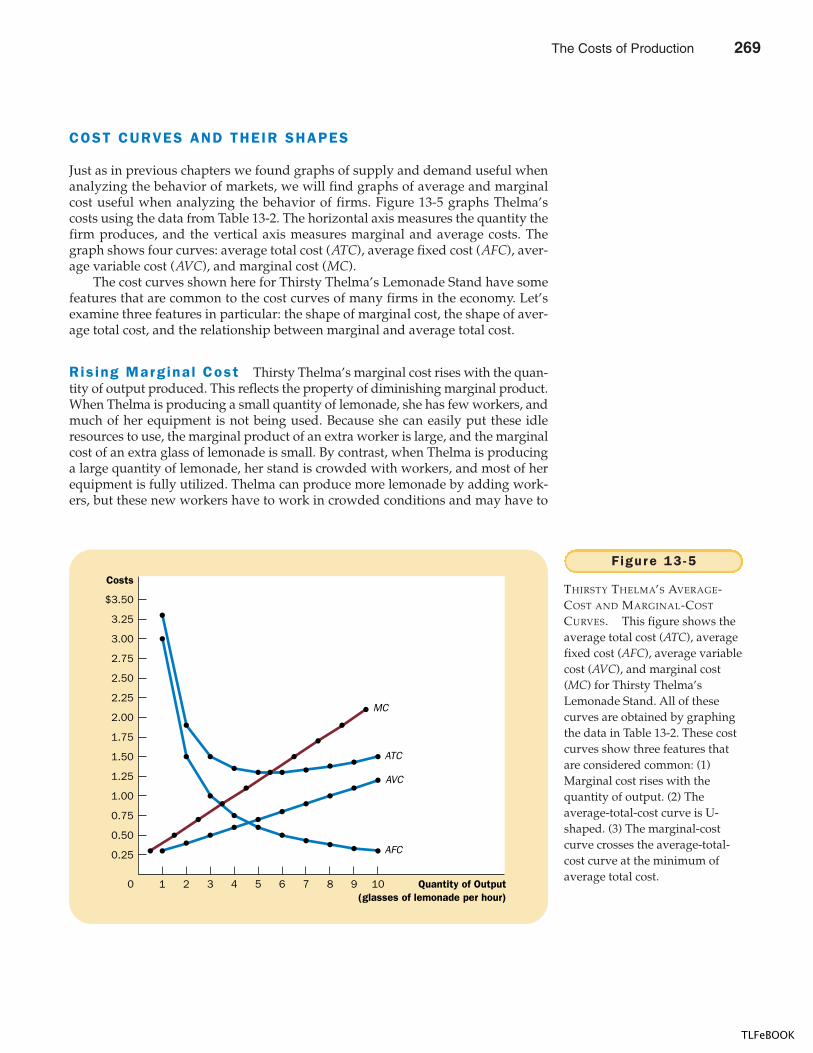
CHAPTER 13 THE COSTS OF PRODUCTION 279
COST CURVES AND THEIR SHAPES
Just as in previous chapters we found graphs of supply and demand useful whenanalyzing the behavior of markets, we will find graphs of average and marginalcost useful when analyzing the behavior of firms. Figure 13-5 graphs Thelma’scosts using the data from Table 13-2. The horizontal axis measures the quantity thefirm produces, and the vertical axis measures marginal and average costs. Thegraph shows four curves: average total cost (ATC), average fixed cost (AFC), aver-age variable cost (AVC), and marginal cost (MC).
The cost curves shown here for Thirsty Thelma’s Lemonade Stand have somefeatures that are common to the cost curves of many firms in the economy. Let’sexamine three features in particular: the shape of marginal cost, the shape of aver-age total cost, and the relationship between marginal and average total cost.
Ris ing Marg ina l Cost Thirsty Thelma’s marginal cost rises with the quan-tity of output produced. This reflects the property of diminishing marginal product.When Thelma is producing a small quantity of lemonade, she has few workers, andmuch of her equipment is not being used. Because she can easily put these idleresources to use, the marginal product of an extra worker is large, and the marginalcost of an extra glass of lemonade is small. By contrast, when Thelma is producinga large quantity of lemonade, her stand is crowded with workers, and most of herequipment is fully utilized. Thelma can produce more lemonade by adding work-ers, but these new workers have to work in crowded conditions and may have to
Costs
$3.50
3.25
3.00
2.75
2.50
2.25
2.00
1.75
1.50
1.25
1.00
0.75
0.50
0.25
Quantity of Output(glasses of lemonade per hour)
0 1 432 765 98 10
MC
ATC
AVC
AFC
Figure 13 -5
THIRSTY THELMA’S AVERAGE-COST AND MARGINAL-COST
CURVES. This figure shows theaverage total cost (ATC), averagefixed cost (AFC), average variablecost (AVC), and marginal cost(MC) for Thirsty Thelma’sLemonade Stand. All of thesecurves are obtained by graphingthe data in Table 13-2. These costcurves show three features thatare considered common: (1)Marginal cost rises with thequantity of output. (2) Theaverage-total-cost curve is U-shaped. (3) The marginal-costcurve crosses the average-total-cost curve at the minimum ofaverage total cost.
The Costs of Production 269
TLFeBOOK
280 PART F IVE FIRM BEHAVIOR AND THE ORGANIZATION OF INDUSTRY
wait to use the equipment. Therefore, when the quantity of lemonade being pro-duced is already high, the marginal product of an extra worker is low, and the mar-ginal cost of an extra glass of lemonade is large.
U-Shaped Average Tota l Cost Thirsty Thelma’s average-total-costcurve is U-shaped. To understand why this is so, remember that average total costis the sum of average fixed cost and average variable cost. Average fixed cost al-ways declines as output rises because the fixed cost is getting spread over a largernumber of units. Average variable cost typically rises as output increases becauseof diminishing marginal product. Average total cost reflects the shapes of both av-erage fixed cost and average variable cost. At very low levels of output, such as 1or 2 glasses per hour, average total cost is high because the fixed cost is spreadover only a few units. Average total cost then declines as output increases until thefirm’s output reaches 5 glasses of lemonade per hour, when average total cost fallsto $1.30 per glass. When the firm produces more than 6 glasses, average total coststarts rising again because average variable cost rises substantially.
The bottom of the U-shape occurs at the quantity that minimizes average totalcost. This quantity is sometimes called the efficient scale of the firm. For ThirstyThelma, the efficient scale is 5 or 6 glasses of lemonade. If she produces more orless than this amount, her average total cost rises above the minimum of $1.30.
The Relat ionship between Marg ina l Cost and Average Tota lCost If you look at Figure 13-5 (or back at Table 13-2), you will see somethingthat may be surprising at first. Whenever marginal cost is less than average total cost,average total cost is falling. Whenever marginal cost is greater than average total cost, av-erage total cost is rising. This feature of Thirsty Thelma’s cost curves is not a coinci-dence from the particular numbers used in the example: It is true for all firms.
To see why, consider an analogy. Average total cost is like your cumulative gradepoint average. Marginal cost is like the grade in the next course you will take. If yourgrade in your next course is less than your grade point average, your grade point av-erage will fall. If your grade in your next course is higher than your grade point av-erage, your grade point average will rise. The mathematics of average and marginalcosts is exactly the same as the mathematics of average and marginal grades.
This relationship between average total cost and marginal cost has an impor-tant corollary: The marginal-cost curve crosses the average-total-cost curve at the efficientscale. Why? At low levels of output, marginal cost is below average total cost, soaverage total cost is falling. But after the two curves cross, marginal cost risesabove average total cost. For the reason we have just discussed, average total costmust start to rise at this level of output. Hence, this point of intersection is the min-imum of average total cost. As you will see in the next chapter, this point of mini-mum average total cost plays a key role in the analysis of competitive firms.
TYPICAL COST CURVES
In the examples we have studied so far, the firms exhibit diminishing marginal prod-uct and, therefore, rising marginal cost at all levels of output. Yet actual firms are of-ten a bit more complicated than this. In many firms, diminishing marginal productdoes not start to occur immediately after the first worker is hired. Depending on the
ef f ic ient sca lethe quantity of output thatminimizes average total cost
270 The Costs of Production
TLFeBOOK
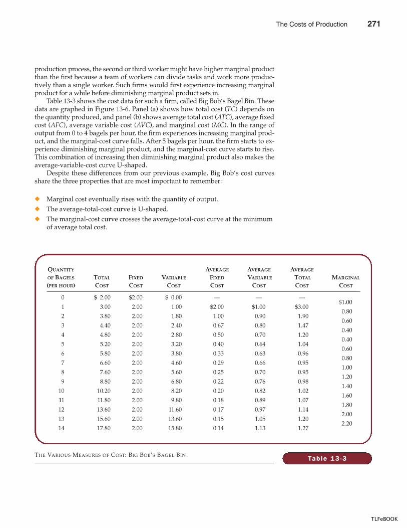
CHAPTER 13 THE COSTS OF PRODUCTION 281
production process, the second or third worker might have higher marginal productthan the first because a team of workers can divide tasks and work more produc-tively than a single worker. Such firms would first experience increasing marginalproduct for a while before diminishing marginal product sets in.
Table 13-3 shows the cost data for such a firm, called Big Bob’s Bagel Bin. Thesedata are graphed in Figure 13-6. Panel (a) shows how total cost (TC) depends onthe quantity produced, and panel (b) shows average total cost (ATC), average fixedcost (AFC), average variable cost (AVC), and marginal cost (MC). In the range ofoutput from 0 to 4 bagels per hour, the firm experiences increasing marginal prod-uct, and the marginal-cost curve falls. After 5 bagels per hour, the firm starts to ex-perience diminishing marginal product, and the marginal-cost curve starts to rise.This combination of increasing then diminishing marginal product also makes theaverage-variable-cost curve U-shaped.
Despite these differences from our previous example, Big Bob’s cost curvesshare the three properties that are most important to remember:
� Marginal cost eventually rises with the quantity of output.� The average-total-cost curve is U-shaped.� The marginal-cost curve crosses the average-total-cost curve at the minimum
of average total cost.
Table 13 -3
QUANTITY AVERAGE AVERAGE AVERAGE
OF BAGELS TOTAL FIXED VARIABLE FIXED VARIABLE TOTAL MARGINAL
(PER HOUR) COST COST COST COST COST COST COST
0 $ 2.00 $2.00 $ 0.00 — — —$1.00
1 3.00 2.00 1.00 $2.00 $1.00 $3.000.80
2 3.80 2.00 1.80 1.00 0.90 1.900.60
3 4.40 2.00 2.40 0.67 0.80 1.470.40
4 4.80 2.00 2.80 0.50 0.70 1.200.40
5 5.20 2.00 3.20 0.40 0.64 1.040.60
6 5.80 2.00 3.80 0.33 0.63 0.960.80
7 6.60 2.00 4.60 0.29 0.66 0.951.00
8 7.60 2.00 5.60 0.25 0.70 0.951.20
9 8.80 2.00 6.80 0.22 0.76 0.981.40
10 10.20 2.00 8.20 0.20 0.82 1.021.60
11 11.80 2.00 9.80 0.18 0.89 1.071.80
12 13.60 2.00 11.60 0.17 0.97 1.142.00
13 15.60 2.00 13.60 0.15 1.05 1.202.20
14 17.80 2.00 15.80 0.14 1.13 1.27
THE VARIOUS MEASURES OF COST: BIG BOB’S BAGEL BIN
The Costs of Production 271
TLFeBOOK
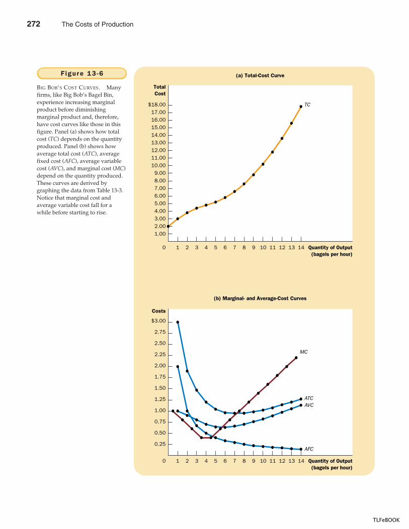
282 PART F IVE FIRM BEHAVIOR AND THE ORGANIZATION OF INDUSTRY
0
(a) Total-Cost Curve
(b) Marginal- and Average-Cost Curves
TotalCost
$18.0017.0016.0015.0014.0013.0012.0011.0010.00
9.008.007.006.005.004.003.00
Quantity of Output(bagels per hour)
TC
Quantity of Output(bagels per hour)
1 432 765 98 1413121110
2.001.00
Costs
$3.00
2.75
2.50
2.25
2.00
1.75
1.50
1.25
1.00
0.75
0.50
0.25
0 1 432 765 98 1413121110
MC
ATCAVC
AFC
BIG BOB’S COST CURVES. Manyfirms, like Big Bob’s Bagel Bin,experience increasing marginalproduct before diminishingmarginal product and, therefore,have cost curves like those in thisfigure. Panel (a) shows how totalcost (TC) depends on the quantityproduced. Panel (b) shows howaverage total cost (ATC), averagefixed cost (AFC), average variablecost (AVC), and marginal cost (MC)depend on the quantity produced.These curves are derived bygraphing the data from Table 13-3.Notice that marginal cost andaverage variable cost fall for awhile before starting to rise.
Figure 13 -6
272 The Costs of Production
TLFeBOOK
CHAPTER 13 THE COSTS OF PRODUCTION 283
QUICK QUIZ: Suppose Honda’s total cost of producing 4 cars is $225,000 and its total cost of producing 5 cars is $250,000. What is the average total costof producing 5 cars? What is the marginal cost of the fifth car? � Draw themarginal-cost curve and the average-total-cost curve for a typical firm, and explain why these curves cross where they do.
COSTS IN THE SHORT RUN AND IN THE LONG RUN
We noted at the beginning of this chapter that a firm’s costs might depend onthe time horizon being examined. Let’s examine more precisely why this might bethe case.
THE RELATIONSHIP BETWEEN SHORT-RUN AND LONG-RUN AVERAGE TOTAL COST
For many firms, the division of total costs between fixed and variable costs de-pends on the time horizon. Consider, for instance, a car manufacturer, such as FordMotor Company. Over a period of only a few months, Ford cannot adjust the num-ber or sizes of its car factories. The only way it can produce additional cars is tohire more workers at the factories it already has. The cost of these factories is,therefore, a fixed cost in the short run. By contrast, over a period of several years,Ford can expand the size of its factories, build new factories, or close old ones.Thus, the cost of its factories is a variable cost in the long run.
Because many decisions are fixed in the short run but variable in the long run,a firm’s long-run cost curves differ from its short-run cost curves. Figure 13-7shows an example. The figure presents three short-run average-total-cost curves—for a small, medium, and large factory. It also presents the long-run average-total-cost curve. As the firm moves along the long-run curve, it is adjusting the size ofthe factory to the quantity of production.
This graph shows how short-run and long-run costs are related. The long-runaverage-total-cost curve is a much flatter U-shape than the short-run average-total-cost curve. In addition, all the short-run curves lie on or above the long-run curve.These properties arise because of the greater flexibility firms have in the long run.In essence, in the long run, the firm gets to choose which short-run curve it wantsto use. But in the short run, it has to use whatever short-run curve it chose inthe past.
The figure shows an example of how a change in production alters costs overdifferent time horizons. When Ford wants to increase production from 1,000 to1,200 cars per day, it has no choice in the short run but to hire more workers at itsexisting medium-sized factory. Because of diminishing marginal product, averagetotal cost rises from $10,000 to $12,000 per car. In the long run, however, Ford canexpand both the size of the factory and its workforce, and average total cost re-mains at $10,000.
How long does it take for a firm to get to the long run? The answer dependson the firm. It can take a year or longer for a major manufacturing firm, such as a
The Costs of Production 273
TLFeBOOK
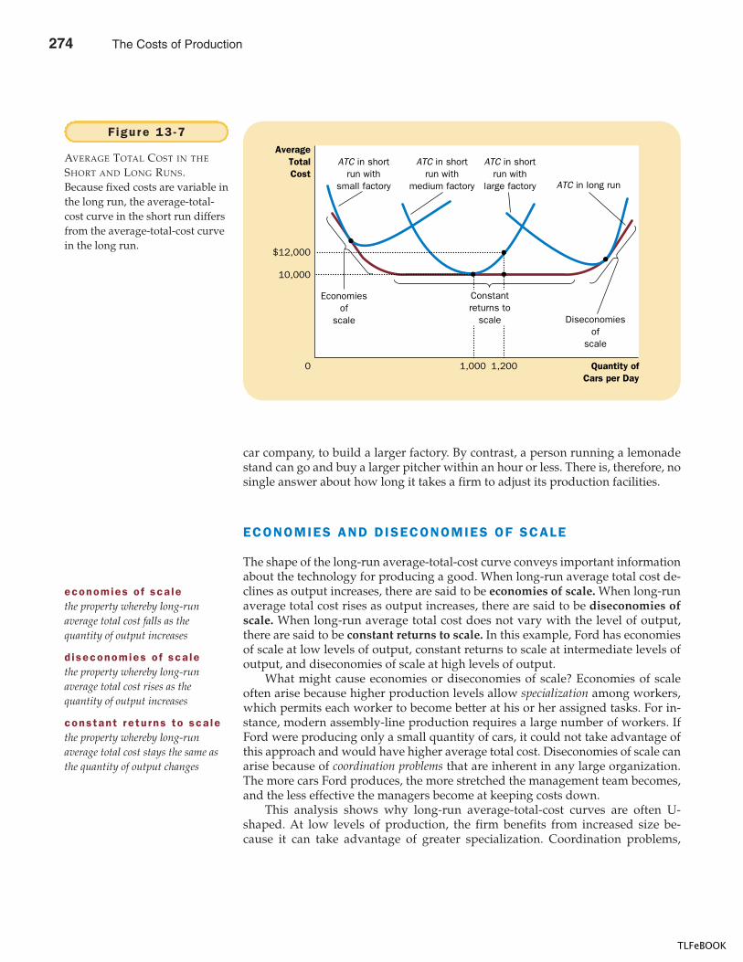
284 PART F IVE FIRM BEHAVIOR AND THE ORGANIZATION OF INDUSTRY
car company, to build a larger factory. By contrast, a person running a lemonadestand can go and buy a larger pitcher within an hour or less. There is, therefore, nosingle answer about how long it takes a firm to adjust its production facilities.
ECONOMIES AND DISECONOMIES OF SCALE
The shape of the long-run average-total-cost curve conveys important informationabout the technology for producing a good. When long-run average total cost de-clines as output increases, there are said to be economies of scale. When long-runaverage total cost rises as output increases, there are said to be diseconomies ofscale. When long-run average total cost does not vary with the level of output,there are said to be constant returns to scale. In this example, Ford has economiesof scale at low levels of output, constant returns to scale at intermediate levels ofoutput, and diseconomies of scale at high levels of output.
What might cause economies or diseconomies of scale? Economies of scaleoften arise because higher production levels allow specialization among workers,which permits each worker to become better at his or her assigned tasks. For in-stance, modern assembly-line production requires a large number of workers. IfFord were producing only a small quantity of cars, it could not take advantage ofthis approach and would have higher average total cost. Diseconomies of scale canarise because of coordination problems that are inherent in any large organization.The more cars Ford produces, the more stretched the management team becomes,and the less effective the managers become at keeping costs down.
This analysis shows why long-run average-total-cost curves are often U-shaped. At low levels of production, the firm benefits from increased size be-cause it can take advantage of greater specialization. Coordination problems,
Quantity ofCars per Day
0 1,2001,000
AverageTotalCost
$12,000
10,000
Economiesof
scale
ATC in shortrun with
small factory
ATC in shortrun with
medium factory
ATC in shortrun with
large factory ATC in long run
Diseconomiesof
scale
Constantreturns to
scale
Figure 13 -7
AVERAGE TOTAL COST IN THE
SHORT AND LONG RUNS.Because fixed costs are variable inthe long run, the average-total-cost curve in the short run differsfrom the average-total-cost curvein the long run.
economies o f sca lethe property whereby long-runaverage total cost falls as thequantity of output increases
diseconomies o f sca lethe property whereby long-runaverage total cost rises as thequantity of output increases
constant r eturns to sca lethe property whereby long-runaverage total cost stays the same asthe quantity of output changes
274 The Costs of Production
TLFeBOOK
CHAPTER 13 THE COSTS OF PRODUCTION 285
meanwhile, are not yet acute. By contrast, at high levels of production, the benefitsof specialization have already been realized, and coordination problems becomemore severe as the firm grows larger. Thus, long-run average total cost is falling atlow levels of production because of increasing specialization and rising at highlevels of production because of increasing coordination problems.
QUICK QUIZ: If Boeing produces 9 jets per month, its long-run total cost is $9.0 million per month. If it produces 10 jets per month, its long-run total cost is $9.5 million per month. Does Boeing exhibit economies or diseconomies of scale?
CONCLUSION
The purpose of this chapter has been to develop some tools that we can use to studyhow firms make production and pricing decisions. You should now understandwhat economists mean by the term costs and how costs vary with the quantity ofoutput a firm produces. To refresh your memory, Table 13-4 summarizes some ofthe definitions we have encountered.
“Jack of all trades, master ofnone.” This well-known adagehelps explain why firms some-times experience economies ofscale. A person who tries to doeverything usually ends up doingnothing very well. If a firm wantsits workers to be as productiveas they can be, it is often bestto give them a limited task thatthey can master. But this is pos-sible only if a firm employs alarge number of workers and
produces a large quantity of output.In his celebrated book, An Inquiry into the Nature and
Causes of the Wealth of Nations, Adam Smith described anexample of this based on a visit he made to a pin factory.Smith was impressed by the specialization among the work-ers that he observed and the resulting economies of scale.He wrote,
“One man draws out the wire, another straightens it, athird cuts it, a fourth points it, a fifth grinds it at the top
for receiving the head; to make the head requires two orthree distinct operations; to put it on is a peculiarbusiness; to whiten it is another; it is even a trade byitself to put them into paper.”
Smith reported that because of this specialization, the pinfactory produced thousands of pins per worker every day.He conjectured that if the workers had chosen to work sep-arately, rather than as a team of specialists, “they certainlycould not each of them make twenty, perhaps not one pin aday.” In other words, because of specialization, a large pinfactory could achieve higher output per worker and lower av-erage cost per pin than a small pin factory.
The specialization that Smith observed in the pin fac-tory is prevalent in the modern economy. If you want to builda house, for instance, you could try to do all the work your-self. But most people turn to a builder, who in turn hirescarpenters, plumbers, electricians, painters, and many othertypes of worker. These workers specialize in particular jobs,and this allows them to become better at their jobs than ifthey were generalists. Indeed, the use of specialization toachieve economies of scale is one reason modern societiesare as prosperous as they are.
FYI
Lessons from a
Pin Factory
The Costs of Production 275
TLFeBOOK
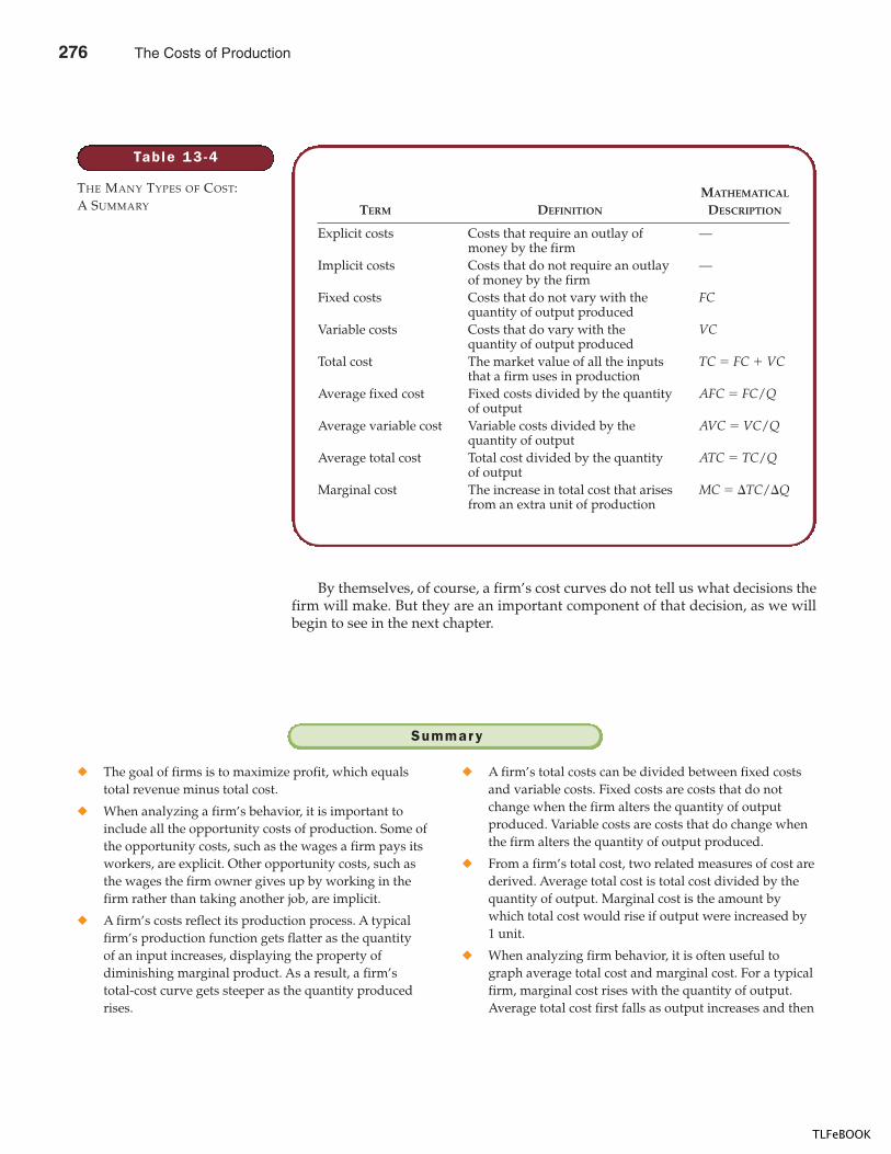
286 PART F IVE FIRM BEHAVIOR AND THE ORGANIZATION OF INDUSTRY
By themselves, of course, a firm’s cost curves do not tell us what decisions thefirm will make. But they are an important component of that decision, as we willbegin to see in the next chapter.
Table 13 -4
THE MANY TYPES OF COST:A SUMMARY
MATHEMATICAL
TERM DEFINITION DESCRIPTION
Explicit costs Costs that require an outlay of —money by the firm
Implicit costs Costs that do not require an outlay —of money by the firm
Fixed costs Costs that do not vary with the FCquantity of output produced
Variable costs Costs that do vary with the VCquantity of output produced
Total cost The market value of all the inputs TC � FC � VCthat a firm uses in production
Average fixed cost Fixed costs divided by the quantity AFC � FC/Qof output
Average variable cost Variable costs divided by the AVC � VC/Qquantity of output
Average total cost Total cost divided by the quantity ATC � TC/Qof output
Marginal cost The increase in total cost that arises MC � �TC/�Qfrom an extra unit of production
� The goal of firms is to maximize profit, which equalstotal revenue minus total cost.
� When analyzing a firm’s behavior, it is important toinclude all the opportunity costs of production. Some ofthe opportunity costs, such as the wages a firm pays itsworkers, are explicit. Other opportunity costs, such asthe wages the firm owner gives up by working in thefirm rather than taking another job, are implicit.
� A firm’s costs reflect its production process. A typicalfirm’s production function gets flatter as the quantityof an input increases, displaying the property ofdiminishing marginal product. As a result, a firm’s total-cost curve gets steeper as the quantity producedrises.
� A firm’s total costs can be divided between fixed costsand variable costs. Fixed costs are costs that do notchange when the firm alters the quantity of outputproduced. Variable costs are costs that do change whenthe firm alters the quantity of output produced.
� From a firm’s total cost, two related measures of cost arederived. Average total cost is total cost divided by thequantity of output. Marginal cost is the amount bywhich total cost would rise if output were increased by1 unit.
� When analyzing firm behavior, it is often useful tograph average total cost and marginal cost. For a typicalfirm, marginal cost rises with the quantity of output.Average total cost first falls as output increases and then
Summar y
276 The Costs of Production
TLFeBOOK
CHAPTER 13 THE COSTS OF PRODUCTION 287
rises as output increases further. The marginal-costcurve always crosses the average-total-cost curve at theminimum of average total cost.
� A firm’s costs often depend on the time horizon beingconsidered. In particular, many costs are fixed in the
short run but variable in the long run. As a result, whenthe firm changes its level of production, average totalcost may rise more in the short run than in the long run.
total revenue, p. 270total cost, p. 270profit, p. 270explicit costs, p. 271implicit costs, p. 271economic profit, p. 272accounting profit, p. 272
production function, p. 273marginal product, p. 273diminishing marginal product, p. 273fixed costs, p. 277variable costs, p. 277average total cost, p. 278average fixed cost, p. 278
average variable cost, p. 278marginal cost, p. 278efficient scale, p. 280economies of scale, p. 284diseconomies of scale, p. 284constant returns to scale, p. 284
Key Concepts
1. What is the relationship between a firm’s total revenue,profit, and total cost?
2. Give an example of an opportunity cost that anaccountant might not count as a cost. Why would theaccountant ignore this cost?
3. What is marginal product, and what does it mean if it isdiminishing?
4. Draw a production function that exhibits diminishingmarginal product of labor. Draw the associated total-cost curve. (In both cases, be sure to label the axes.)Explain the shapes of the two curves you have drawn.
5. Define total cost, average total cost, and marginal cost.How are they related?
6. Draw the marginal-cost and average-total-cost curvesfor a typical firm. Explain why the curves have theshapes that they do and why they cross where they do.
7. How and why does a firm’s average-total-cost curvediffer in the short run and in the long run?
8. Define economies of scale and explain why they mightarise. Define diseconomies of scale and explain why theymight arise.
Quest ions fo r Rev iew
1. This chapter discusses many types of costs: opportunitycost, total cost, fixed cost, variable cost, average totalcost, and marginal cost. Fill in the type of cost that bestcompletes the phrases below:a. The true cost of taking some action is its _______.b. _______ is falling when marginal cost is below it,
and rising when marginal cost is above it.c. A cost that does not depend on the quantity
produced is a _______.d. In the ice-cream industry in the short run, _______
includes the cost of cream and sugar, but not thecost of the factory.
e. Profits equal total revenue less _______.f. The cost of producing an extra unit of output is
_______.
2. Your aunt is thinking about opening a hardware store.She estimates that it would cost $500,000 per year to rentthe location and buy the stock. In addition, she wouldhave to quit her $50,000 per year job as an accountant.a. Define opportunity cost.b. What is your aunt’s opportunity cost of running a
hardware store for a year? If your aunt thought shecould sell $510,000 worth of merchandise in a year,should she open the store? Explain.
Prob lems and App l icat ions
The Costs of Production 277
TLFeBOOK
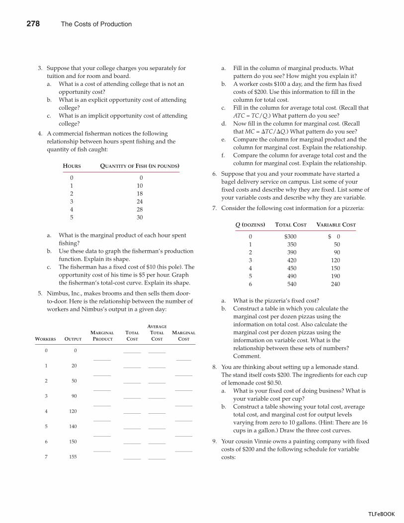
288 PART F IVE FIRM BEHAVIOR AND THE ORGANIZATION OF INDUSTRY
3. Suppose that your college charges you separately fortuition and for room and board.a. What is a cost of attending college that is not an
opportunity cost?b. What is an explicit opportunity cost of attending
college?c. What is an implicit opportunity cost of attending
college?
4. A commercial fisherman notices the followingrelationship between hours spent fishing and thequantity of fish caught:
HOURS QUANTITY OF FISH (IN POUNDS)
0 01 102 183 244 285 30
a. What is the marginal product of each hour spentfishing?
b. Use these data to graph the fisherman’s productionfunction. Explain its shape.
c. The fisherman has a fixed cost of $10 (his pole). Theopportunity cost of his time is $5 per hour. Graphthe fisherman’s total-cost curve. Explain its shape.
5. Nimbus, Inc., makes brooms and then sells them door-to-door. Here is the relationship between the number ofworkers and Nimbus’s output in a given day:
AVERAGE
MARGINAL TOTAL TOTAL MARGINAL
WORKERS OUTPUT PRODUCT COST COST COST
0 0 _______ _______
_______ ______
1 20 _______ _______
_______ _______
2 50 _______ _______
_______ _______
3 90 _______ _______
_______ _______
4 120 _______ _______
_______ _______
5 140 _______ _______
_______ _______
6 150 _______ _______
_______ _______
7 155 _______ _______
a. Fill in the column of marginal products. Whatpattern do you see? How might you explain it?
b. A worker costs $100 a day, and the firm has fixedcosts of $200. Use this information to fill in thecolumn for total cost.
c. Fill in the column for average total cost. (Recall thatATC = TC/Q.) What pattern do you see?
d. Now fill in the column for marginal cost. (Recallthat MC = �TC/�Q.) What pattern do you see?
e. Compare the column for marginal product and thecolumn for marginal cost. Explain the relationship.
f. Compare the column for average total cost and thecolumn for marginal cost. Explain the relationship.
6. Suppose that you and your roommate have started abagel delivery service on campus. List some of yourfixed costs and describe why they are fixed. List some ofyour variable costs and describe why they are variable.
7. Consider the following cost information for a pizzeria:
Q (DOZENS) TOTAL COST VARIABLE COST
0 $300 $ 01 350 502 390 903 420 1204 450 1505 490 1906 540 240
a. What is the pizzeria’s fixed cost?b. Construct a table in which you calculate the
marginal cost per dozen pizzas using theinformation on total cost. Also calculate themarginal cost per dozen pizzas using theinformation on variable cost. What is therelationship between these sets of numbers?Comment.
8. You are thinking about setting up a lemonade stand.The stand itself costs $200. The ingredients for each cupof lemonade cost $0.50.a. What is your fixed cost of doing business? What is
your variable cost per cup?b. Construct a table showing your total cost, average
total cost, and marginal cost for output levelsvarying from zero to 10 gallons. (Hint: There are 16cups in a gallon.) Draw the three cost curves.
9. Your cousin Vinnie owns a painting company with fixedcosts of $200 and the following schedule for variablecosts:
278 The Costs of Production
TLFeBOOK
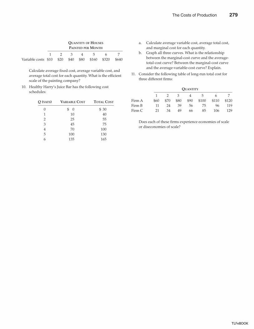
CHAPTER 13 THE COSTS OF PRODUCTION 289
QUANTITY OF HOUSES
PAINTED PER MONTH
1 2 3 4 5 6 7Variable costs $10 $20 $40 $80 $160 $320 $640
Calculate average fixed cost, average variable cost, andaverage total cost for each quantity. What is the efficientscale of the painting company?
10. Healthy Harry’s Juice Bar has the following costschedules:
Q (VATS) VARIABLE COST TOTAL COST
0 $ 0 $ 301 10 402 25 553 45 754 70 1005 100 1306 135 165
a. Calculate average variable cost, average total cost,and marginal cost for each quantity.
b. Graph all three curves. What is the relationshipbetween the marginal-cost curve and the average-total-cost curve? Between the marginal-cost curveand the average-variable-cost curve? Explain.
11. Consider the following table of long-run total cost forthree different firms:
QUANTITY
1 2 3 4 5 6 7Firm A $60 $70 $80 $90 $100 $110 $120Firm B 11 24 39 56 75 96 119Firm C 21 34 49 66 85 106 129
Does each of these firms experience economies of scaleor diseconomies of scale?
The Costs of Production 279
TLFeBOOK

TLFeBOOK

IN THIS CHAPTERYOU WILL . . .
See how f i rmbehav ior determines
a market ’s shor t -r un and long - r un
supp ly cur ves
Examine howcompet i t i ve f i rms
decide when to shutdown product ion
temporar i l y
Learn whatcharacter ist icsmake a market
compet i t i ve
Examine howcompet i t i ve f i rmsdecide how muchoutput to produce
Examine howcompet i t i ve f i rms
decide whetherto ex i t o r enter
a market
If your local gas station raised the price it charges for gasoline by 20 percent, itwould see a large drop in the amount of gasoline it sold. Its customers wouldquickly switch to buying their gasoline at other gas stations. By contrast, if your lo-cal water company raised the price of water by 20 percent, it would see only asmall decrease in the amount of water it sold. People might water their lawns lessoften and buy more water-efficient shower heads, but they would be hard-pressedto reduce water consumption greatly and would be unlikely to find another sup-plier. The difference between the gasoline market and the water market is obvious:There are many firms pumping gasoline, but there is only one firm pumping wa-ter. As you might expect, this difference in market structure shapes the pricing andproduction decisions of the firms that operate in these markets.
In this chapter we examine the behavior of competitive firms, such as your lo-cal gas station. You may recall that a market is competitive if each buyer and seller
F I R M S I N
C O M P E T I T I V E M A R K E T S
291
281
14
TLFeBOOK
292 PART F IVE FIRM BEHAVIOR AND THE ORGANIZATION OF INDUSTRY
is small compared to the size of the market and, therefore, has little ability to in-fluence market prices. By contrast, if a firm can influence the market price of thegood it sells, it is said to have market power. In the three chapters that follow thisone, we examine the behavior of firms with market power, such as your local wa-ter company.
Our analysis of competitive firms in this chapter will shed light on the deci-sions that lie behind the supply curve in a competitive market. Not surprisingly,we will find that a market supply curve is tightly linked to firms’ costs of produc-tion. (Indeed, this general insight should be familiar to you from our analysis inChapter 7.) But among a firm’s various costs—fixed, variable, average, and mar-ginal—which ones are most relevant for its decision about the quantity to sup-ply? We will see that all these measures of cost play important and interrelatedroles.
WHAT IS A COMPETIT IVE MARKET?
Our goal in this chapter is to examine how firms make production decisions incompetitive markets. As a background for this analysis, we begin by consideringwhat a competitive market is.
THE MEANING OF COMPETIT ION
Although we have already discussed the meaning of competition in Chapter 4,let’s review the lesson briefly. A competitive market, sometimes called a perfectlycompetitive market, has two characteristics:
� There are many buyers and many sellers in the market.� The goods offered by the various sellers are largely the same.
As a result of these conditions, the actions of any single buyer or seller in the mar-ket have a negligible impact on the market price. Each buyer and seller takes themarket price as given.
An example is the market for milk. No single buyer of milk can influence theprice of milk because each buyer purchases a small amount relative to the size ofthe market. Similarly, each seller of milk has limited control over the price becausemany other sellers are offering milk that is essentially identical. Because each sellercan sell all he wants at the going price, he has little reason to charge less, and if hecharges more, buyers will go elsewhere. Buyers and sellers in competitive marketsmust accept the price the market determines and, therefore, are said to be pricetakers.
In addition to the foregoing two conditions for competition, there is a thirdcondition sometimes thought to characterize perfectly competitive markets:
� Firms can freely enter or exit the market.
compet i t i ve marketa market with many buyers andsellers trading identical productsso that each buyer and seller is aprice taker
282 Firms in Competitive Markets
TLFeBOOK
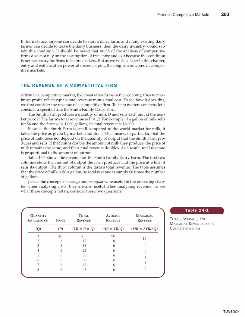
CHAPTER 14 FIRMS IN COMPETIT IVE MARKETS 293
If, for instance, anyone can decide to start a dairy farm, and if any existing dairyfarmer can decide to leave the dairy business, then the dairy industry would sat-isfy this condition. It should be noted that much of the analysis of competitivefirms does not rely on the assumption of free entry and exit because this conditionis not necessary for firms to be price takers. But as we will see later in this chapter,entry and exit are often powerful forces shaping the long-run outcome in compet-itive markets.
THE REVENUE OF A COMPETIT IVE F IRM
A firm in a competitive market, like most other firms in the economy, tries to max-imize profit, which equals total revenue minus total cost. To see how it does this,we first consider the revenue of a competitive firm. To keep matters concrete, let’sconsider a specific firm: the Smith Family Dairy Farm.
The Smith Farm produces a quantity of milk Q and sells each unit at the mar-ket price P. The farm’s total revenue is P � Q. For example, if a gallon of milk sellsfor $6 and the farm sells 1,000 gallons, its total revenue is $6,000.
Because the Smith Farm is small compared to the world market for milk, ittakes the price as given by market conditions. This means, in particular, that theprice of milk does not depend on the quantity of output that the Smith Farm pro-duces and sells. If the Smiths double the amount of milk they produce, the price ofmilk remains the same, and their total revenue doubles. As a result, total revenueis proportional to the amount of output.
Table 14-1 shows the revenue for the Smith Family Dairy Farm. The first twocolumns show the amount of output the farm produces and the price at which itsells its output. The third column is the farm’s total revenue. The table assumesthat the price of milk is $6 a gallon, so total revenue is simply $6 times the numberof gallons.
Just as the concepts of average and marginal were useful in the preceding chap-ter when analyzing costs, they are also useful when analyzing revenue. To seewhat these concepts tell us, consider these two questions:
Table 14 -1
TOTAL, AVERAGE, AND
MARGINAL REVENUE FOR A
COMPETITIVE FIRM
QUANTITY TOTAL AVERAGE MARGINAL
(IN GALLONS) PRICE REVENUE REVENUE REVENUE
(Q) (P) (TR � P � Q) (AR � TR/Q) (MR � ∆TR/∆Q)
1 $6 $ 6 $6$6
2 6 12 66
3 6 18 66
4 6 24 66
5 6 30 66
6 6 36 66
7 6 42 66
8 6 48 6
Firms in Competitive Markets 283
TLFeBOOK
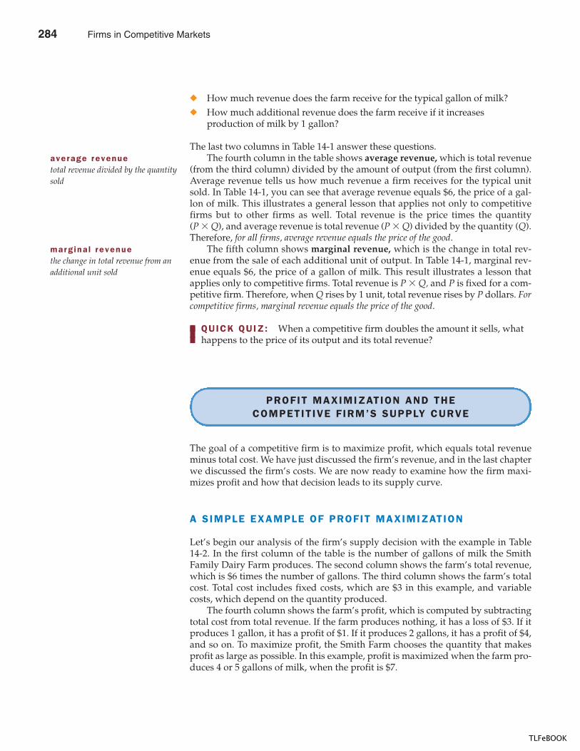
294 PART F IVE FIRM BEHAVIOR AND THE ORGANIZATION OF INDUSTRY
� How much revenue does the farm receive for the typical gallon of milk?� How much additional revenue does the farm receive if it increases
production of milk by 1 gallon?
The last two columns in Table 14-1 answer these questions.The fourth column in the table shows average revenue, which is total revenue
(from the third column) divided by the amount of output (from the first column).Average revenue tells us how much revenue a firm receives for the typical unitsold. In Table 14-1, you can see that average revenue equals $6, the price of a gal-lon of milk. This illustrates a general lesson that applies not only to competitivefirms but to other firms as well. Total revenue is the price times the quantity(P � Q), and average revenue is total revenue (P � Q) divided by the quantity (Q).Therefore, for all firms, average revenue equals the price of the good.
The fifth column shows marginal revenue, which is the change in total rev-enue from the sale of each additional unit of output. In Table 14-1, marginal rev-enue equals $6, the price of a gallon of milk. This result illustrates a lesson thatapplies only to competitive firms. Total revenue is P � Q, and P is fixed for a com-petitive firm. Therefore, when Q rises by 1 unit, total revenue rises by P dollars. Forcompetitive firms, marginal revenue equals the price of the good.
QUICK QUIZ: When a competitive firm doubles the amount it sells, what happens to the price of its output and its total revenue?
PROFIT MAXIMIZATION AND THECOMPETIT IVE FIRM’S SUPPLY CURVE
The goal of a competitive firm is to maximize profit, which equals total revenueminus total cost. We have just discussed the firm’s revenue, and in the last chapterwe discussed the firm’s costs. We are now ready to examine how the firm maxi-mizes profit and how that decision leads to its supply curve.
A SIMPLE EXAMPLE OF PROFIT MAXIMIZATION
Let’s begin our analysis of the firm’s supply decision with the example in Table14-2. In the first column of the table is the number of gallons of milk the SmithFamily Dairy Farm produces. The second column shows the farm’s total revenue,which is $6 times the number of gallons. The third column shows the farm’s totalcost. Total cost includes fixed costs, which are $3 in this example, and variablecosts, which depend on the quantity produced.
The fourth column shows the farm’s profit, which is computed by subtractingtotal cost from total revenue. If the farm produces nothing, it has a loss of $3. If itproduces 1 gallon, it has a profit of $1. If it produces 2 gallons, it has a profit of $4,and so on. To maximize profit, the Smith Farm chooses the quantity that makesprofit as large as possible. In this example, profit is maximized when the farm pro-duces 4 or 5 gallons of milk, when the profit is $7.
average r evenuetotal revenue divided by the quantitysold
marg ina l r evenuethe change in total revenue from anadditional unit sold
284 Firms in Competitive Markets
TLFeBOOK
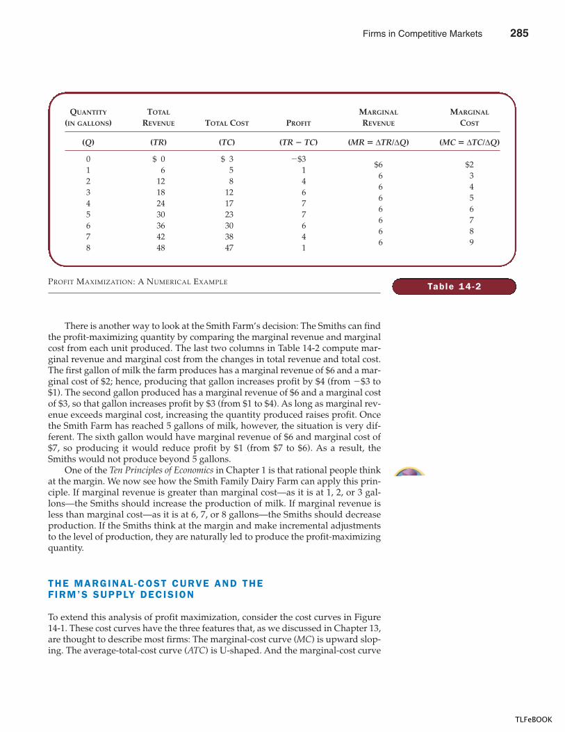
CHAPTER 14 FIRMS IN COMPETIT IVE MARKETS 295
There is another way to look at the Smith Farm’s decision: The Smiths can findthe profit-maximizing quantity by comparing the marginal revenue and marginalcost from each unit produced. The last two columns in Table 14-2 compute mar-ginal revenue and marginal cost from the changes in total revenue and total cost.The first gallon of milk the farm produces has a marginal revenue of $6 and a mar-ginal cost of $2; hence, producing that gallon increases profit by $4 (from �$3 to$1). The second gallon produced has a marginal revenue of $6 and a marginal costof $3, so that gallon increases profit by $3 (from $1 to $4). As long as marginal rev-enue exceeds marginal cost, increasing the quantity produced raises profit. Oncethe Smith Farm has reached 5 gallons of milk, however, the situation is very dif-ferent. The sixth gallon would have marginal revenue of $6 and marginal cost of$7, so producing it would reduce profit by $1 (from $7 to $6). As a result, theSmiths would not produce beyond 5 gallons.
One of the Ten Principles of Economics in Chapter 1 is that rational people thinkat the margin. We now see how the Smith Family Dairy Farm can apply this prin-ciple. If marginal revenue is greater than marginal cost—as it is at 1, 2, or 3 gal-lons—the Smiths should increase the production of milk. If marginal revenue isless than marginal cost—as it is at 6, 7, or 8 gallons—the Smiths should decreaseproduction. If the Smiths think at the margin and make incremental adjustmentsto the level of production, they are naturally led to produce the profit-maximizingquantity.
THE MARGINAL -COST CURVE AND THEFIRM’S SUPPLY DECISION
To extend this analysis of profit maximization, consider the cost curves in Figure14-1. These cost curves have the three features that, as we discussed in Chapter 13,are thought to describe most firms: The marginal-cost curve (MC) is upward slop-ing. The average-total-cost curve (ATC) is U-shaped. And the marginal-cost curve
Table 14 -2
QUANTITY TOTAL MARGINAL MARGINAL
(IN GALLONS) REVENUE TOTAL COST PROFIT REVENUE COST
(Q) (TR) (TC) (TR � TC) (MR � ∆TR/∆Q) (MC � ∆TC/∆Q)
0 $ 0 $ 3 �$3$6 $2
1 6 5 16 3
2 12 8 46 4
3 18 12 66 5
4 24 17 76 6
5 30 23 76 7
6 36 30 66 8
7 42 38 46 9
8 48 47 1
PROFIT MAXIMIZATION: A NUMERICAL EXAMPLE
Firms in Competitive Markets 285
TLFeBOOK
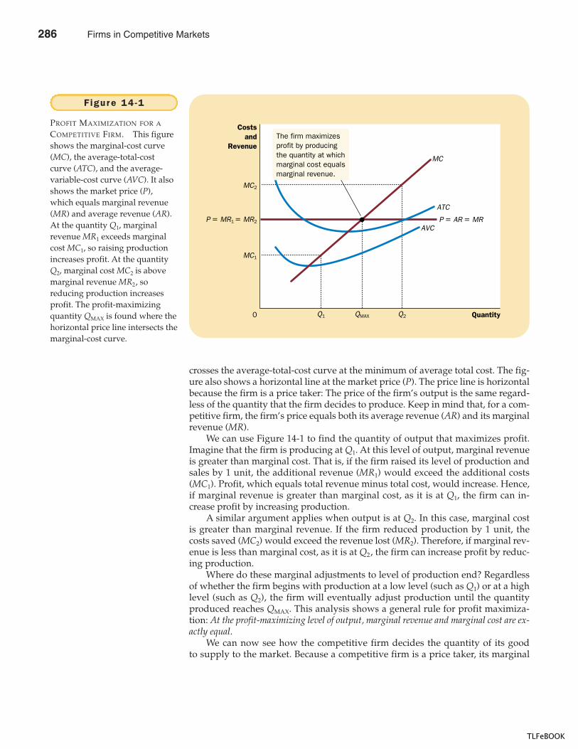
296 PART F IVE FIRM BEHAVIOR AND THE ORGANIZATION OF INDUSTRY
crosses the average-total-cost curve at the minimum of average total cost. The fig-ure also shows a horizontal line at the market price (P). The price line is horizontalbecause the firm is a price taker: The price of the firm’s output is the same regard-less of the quantity that the firm decides to produce. Keep in mind that, for a com-petitive firm, the firm’s price equals both its average revenue (AR) and its marginalrevenue (MR).
We can use Figure 14-1 to find the quantity of output that maximizes profit.Imagine that the firm is producing at Q1. At this level of output, marginal revenueis greater than marginal cost. That is, if the firm raised its level of production andsales by 1 unit, the additional revenue (MR1) would exceed the additional costs(MC1). Profit, which equals total revenue minus total cost, would increase. Hence,if marginal revenue is greater than marginal cost, as it is at Q1, the firm can in-crease profit by increasing production.
A similar argument applies when output is at Q2. In this case, marginal costis greater than marginal revenue. If the firm reduced production by 1 unit, thecosts saved (MC2) would exceed the revenue lost (MR2). Therefore, if marginal rev-enue is less than marginal cost, as it is at Q2, the firm can increase profit by reduc-ing production.
Where do these marginal adjustments to level of production end? Regardlessof whether the firm begins with production at a low level (such as Q1) or at a highlevel (such as Q2), the firm will eventually adjust production until the quantityproduced reaches QMAX. This analysis shows a general rule for profit maximiza-tion: At the profit-maximizing level of output, marginal revenue and marginal cost are ex-actly equal.
We can now see how the competitive firm decides the quantity of its goodto supply to the market. Because a competitive firm is a price taker, its marginal
Quantity0
Costsand
Revenue
MC
ATC
AVC
MC2
MC1
Q1 Q2QMAX
P = MR1 = MR2 P = AR = MR
The firm maximizesprofit by producing the quantity at whichmarginal cost equalsmarginal revenue.
Figure 14 -1
PROFIT MAXIMIZATION FOR A
COMPETITIVE FIRM. This figureshows the marginal-cost curve(MC), the average-total-costcurve (ATC), and the average-variable-cost curve (AVC). It alsoshows the market price (P),which equals marginal revenue(MR) and average revenue (AR).At the quantity Q1, marginalrevenue MR1 exceeds marginalcost MC1, so raising productionincreases profit. At the quantityQ2, marginal cost MC2 is abovemarginal revenue MR2, soreducing production increasesprofit. The profit-maximizingquantity QMAX is found where thehorizontal price line intersects themarginal-cost curve.
286 Firms in Competitive Markets
TLFeBOOK
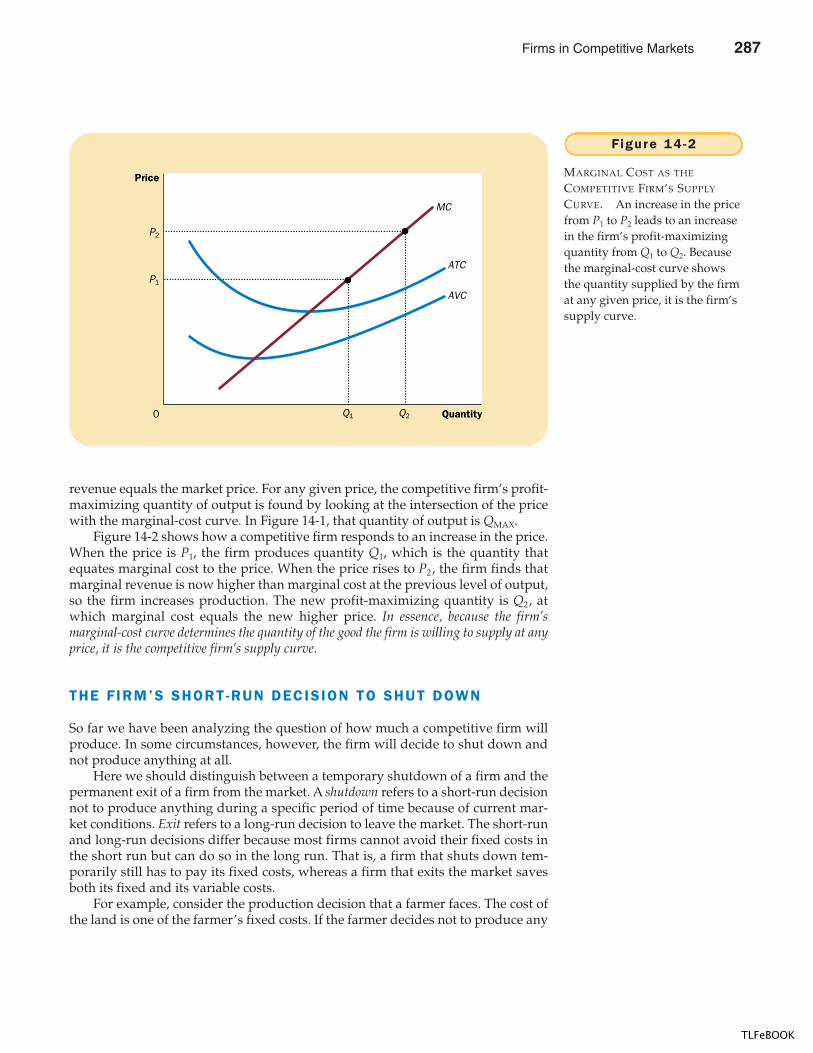
CHAPTER 14 FIRMS IN COMPETIT IVE MARKETS 297
revenue equals the market price. For any given price, the competitive firm’s profit-maximizing quantity of output is found by looking at the intersection of the pricewith the marginal-cost curve. In Figure 14-1, that quantity of output is QMAX.
Figure 14-2 shows how a competitive firm responds to an increase in the price.When the price is P1, the firm produces quantity Q1, which is the quantity thatequates marginal cost to the price. When the price rises to P2, the firm finds thatmarginal revenue is now higher than marginal cost at the previous level of output,so the firm increases production. The new profit-maximizing quantity is Q2, atwhich marginal cost equals the new higher price. In essence, because the firm’smarginal-cost curve determines the quantity of the good the firm is willing to supply at anyprice, it is the competitive firm’s supply curve.
THE F IRM’S SHORT-RUN DECISION TO SHUT DOWN
So far we have been analyzing the question of how much a competitive firm willproduce. In some circumstances, however, the firm will decide to shut down andnot produce anything at all.
Here we should distinguish between a temporary shutdown of a firm and thepermanent exit of a firm from the market. A shutdown refers to a short-run decisionnot to produce anything during a specific period of time because of current mar-ket conditions. Exit refers to a long-run decision to leave the market. The short-runand long-run decisions differ because most firms cannot avoid their fixed costs inthe short run but can do so in the long run. That is, a firm that shuts down tem-porarily still has to pay its fixed costs, whereas a firm that exits the market savesboth its fixed and its variable costs.
For example, consider the production decision that a farmer faces. The cost ofthe land is one of the farmer’s fixed costs. If the farmer decides not to produce any
Quantity0
Price
MC
ATC
AVC
P2
P1
Q1 Q2
Figure 14 -2
MARGINAL COST AS THE
COMPETITIVE FIRM’S SUPPLY
CURVE. An increase in the pricefrom P1 to P2 leads to an increasein the firm’s profit-maximizingquantity from Q1 to Q2. Becausethe marginal-cost curve showsthe quantity supplied by the firmat any given price, it is the firm’ssupply curve.
Firms in Competitive Markets 287
TLFeBOOK
298 PART F IVE FIRM BEHAVIOR AND THE ORGANIZATION OF INDUSTRY
crops one season, the land lies fallow, and he cannot recover this cost. When mak-ing the short-run decision whether to shut down for a season, the fixed cost of landis said to be a sunk cost. By contrast, if the farmer decides to leave farming alto-gether, he can sell the land. When making the long-run decision whether to exit themarket, the cost of land is not sunk. (We return to the issue of sunk costs shortly.)
Now let’s consider what determines a firm’s shutdown decision. If the firmshuts down, it loses all revenue from the sale of its product. At the same time, itsaves the variable costs of making its product (but must still pay the fixed costs).Thus, the firm shuts down if the revenue that it would get from producing is less than itsvariable costs of production.
A small bit of mathematics can make this shutdown criterion more useful. IfTR stands for total revenue, and VC stands for variable costs, then the firm’s deci-sion can be written as
Shut down if TR � VC.
The firm shuts down if total revenue is less than variable cost. By dividing bothsides of this inequality by the quantity Q, we can write it as
Shut down if TR/Q � VC/Q.
Notice that this can be further simplified. TR/Q is total revenue divided by quan-tity, which is average revenue. As we discussed previously, average revenue forany firm is simply the good’s price P. Similarly, VC/Q is average variable costAVC. Therefore, the firm’s shutdown criterion is
Shut down if P � AVC.
That is, a firm chooses to shut down if the price of the good is less than the aver-age variable cost of production. This criterion is intuitive: When choosing to pro-duce, the firm compares the price it receives for the typical unit to the averagevariable cost that it must incur to produce the typical unit. If the price doesn’tcover the average variable cost, the firm is better off stopping production alto-gether. The firm can reopen in the future if conditions change so that price exceedsaverage variable cost.
We now have a full description of a competitive firm’s profit-maximizingstrategy. If the firm produces anything, it produces the quantity at which marginalcost equals the price of the good. Yet if the price is less than average variable costat that quantity, the firm is better off shutting down and not producing anything.These results are illustrated in Figure 14-3. The competitive firm’s short-run supplycurve is the portion of its marginal-cost curve that lies above average variable cost.
SPILT MILK AND OTHER SUNK COSTS
Sometime in your life, you have probably been told, “Don’t cry over spilt milk,” or“Let bygones be bygones.” These adages hold a deep truth about rational decision-making. Economists say that a cost is a sunk cost when it has already been com-mitted and cannot be recovered. In a sense, a sunk cost is the opposite of anopportunity cost: An opportunity cost is what you have to give up if you choose to
sunk costa cost that has already beencommitted and cannot be recovered
288 Firms in Competitive Markets
TLFeBOOK
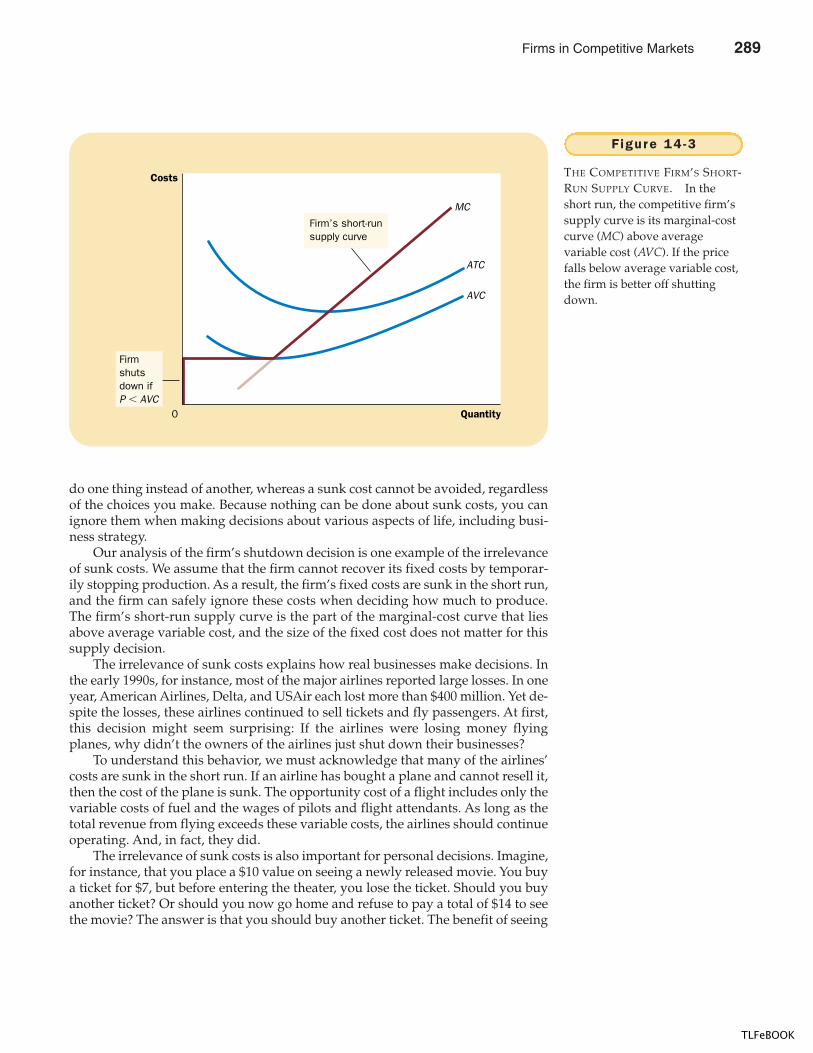
CHAPTER 14 FIRMS IN COMPETIT IVE MARKETS 299
do one thing instead of another, whereas a sunk cost cannot be avoided, regardlessof the choices you make. Because nothing can be done about sunk costs, you canignore them when making decisions about various aspects of life, including busi-ness strategy.
Our analysis of the firm’s shutdown decision is one example of the irrelevanceof sunk costs. We assume that the firm cannot recover its fixed costs by temporar-ily stopping production. As a result, the firm’s fixed costs are sunk in the short run,and the firm can safely ignore these costs when deciding how much to produce.The firm’s short-run supply curve is the part of the marginal-cost curve that liesabove average variable cost, and the size of the fixed cost does not matter for thissupply decision.
The irrelevance of sunk costs explains how real businesses make decisions. Inthe early 1990s, for instance, most of the major airlines reported large losses. In oneyear, American Airlines, Delta, and USAir each lost more than $400 million. Yet de-spite the losses, these airlines continued to sell tickets and fly passengers. At first,this decision might seem surprising: If the airlines were losing money flyingplanes, why didn’t the owners of the airlines just shut down their businesses?
To understand this behavior, we must acknowledge that many of the airlines’costs are sunk in the short run. If an airline has bought a plane and cannot resell it,then the cost of the plane is sunk. The opportunity cost of a flight includes only thevariable costs of fuel and the wages of pilots and flight attendants. As long as thetotal revenue from flying exceeds these variable costs, the airlines should continueoperating. And, in fact, they did.
The irrelevance of sunk costs is also important for personal decisions. Imagine,for instance, that you place a $10 value on seeing a newly released movie. You buya ticket for $7, but before entering the theater, you lose the ticket. Should you buyanother ticket? Or should you now go home and refuse to pay a total of $14 to seethe movie? The answer is that you should buy another ticket. The benefit of seeing
Quantity
MC
ATC
AVC
0
Costs
Firmshutsdown ifP � AVC
Firm’s short-runsupply curve
Figure 14 -3
THE COMPETITIVE FIRM’S SHORT-RUN SUPPLY CURVE. In theshort run, the competitive firm’ssupply curve is its marginal-costcurve (MC) above averagevariable cost (AVC). If the pricefalls below average variable cost,the firm is better off shuttingdown.
Firms in Competitive Markets 289
TLFeBOOK
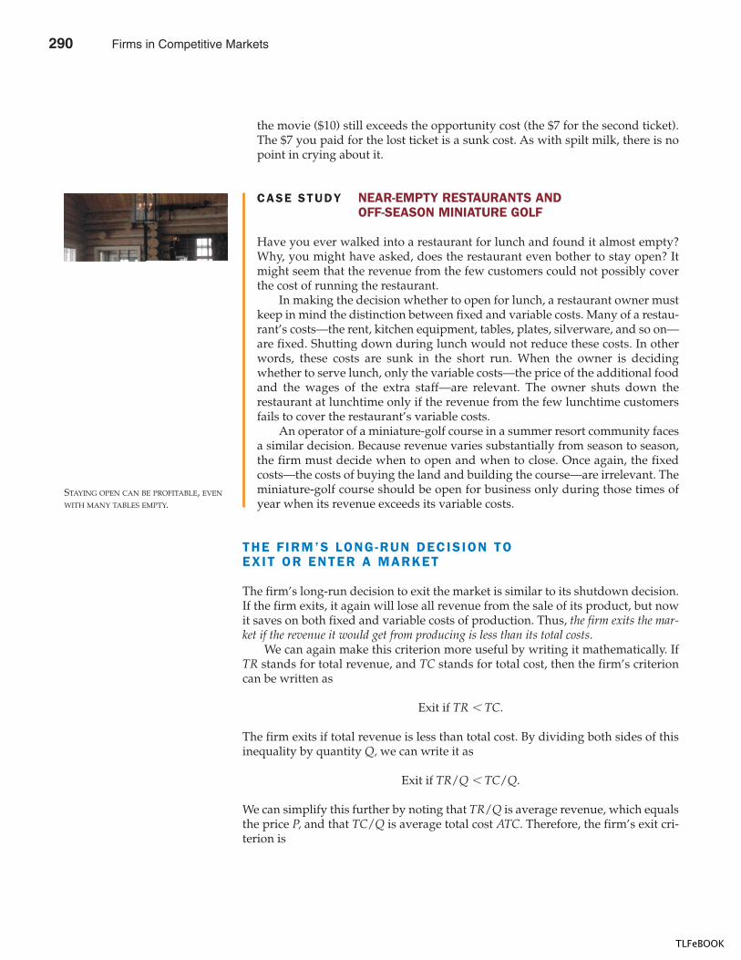
300 PART F IVE FIRM BEHAVIOR AND THE ORGANIZATION OF INDUSTRY
the movie ($10) still exceeds the opportunity cost (the $7 for the second ticket).The $7 you paid for the lost ticket is a sunk cost. As with spilt milk, there is nopoint in crying about it.
CASE STUDY NEAR-EMPTY RESTAURANTS ANDOFF-SEASON MINIATURE GOLF
Have you ever walked into a restaurant for lunch and found it almost empty?Why, you might have asked, does the restaurant even bother to stay open? Itmight seem that the revenue from the few customers could not possibly coverthe cost of running the restaurant.
In making the decision whether to open for lunch, a restaurant owner mustkeep in mind the distinction between fixed and variable costs. Many of a restau-rant’s costs—the rent, kitchen equipment, tables, plates, silverware, and so on—are fixed. Shutting down during lunch would not reduce these costs. In otherwords, these costs are sunk in the short run. When the owner is decidingwhether to serve lunch, only the variable costs—the price of the additional foodand the wages of the extra staff—are relevant. The owner shuts down therestaurant at lunchtime only if the revenue from the few lunchtime customersfails to cover the restaurant’s variable costs.
An operator of a miniature-golf course in a summer resort community facesa similar decision. Because revenue varies substantially from season to season,the firm must decide when to open and when to close. Once again, the fixedcosts—the costs of buying the land and building the course—are irrelevant. Theminiature-golf course should be open for business only during those times ofyear when its revenue exceeds its variable costs.
THE F IRM’S LONG-RUN DECISION TOEXIT OR ENTER A MARKET
The firm’s long-run decision to exit the market is similar to its shutdown decision.If the firm exits, it again will lose all revenue from the sale of its product, but nowit saves on both fixed and variable costs of production. Thus, the firm exits the mar-ket if the revenue it would get from producing is less than its total costs.
We can again make this criterion more useful by writing it mathematically. IfTR stands for total revenue, and TC stands for total cost, then the firm’s criterioncan be written as
Exit if TR � TC.
The firm exits if total revenue is less than total cost. By dividing both sides of thisinequality by quantity Q, we can write it as
Exit if TR/Q � TC/Q.
We can simplify this further by noting that TR/Q is average revenue, which equalsthe price P, and that TC/Q is average total cost ATC. Therefore, the firm’s exit cri-terion is
STAYING OPEN CAN BE PROFITABLE, EVEN
WITH MANY TABLES EMPTY.
290 Firms in Competitive Markets
TLFeBOOK
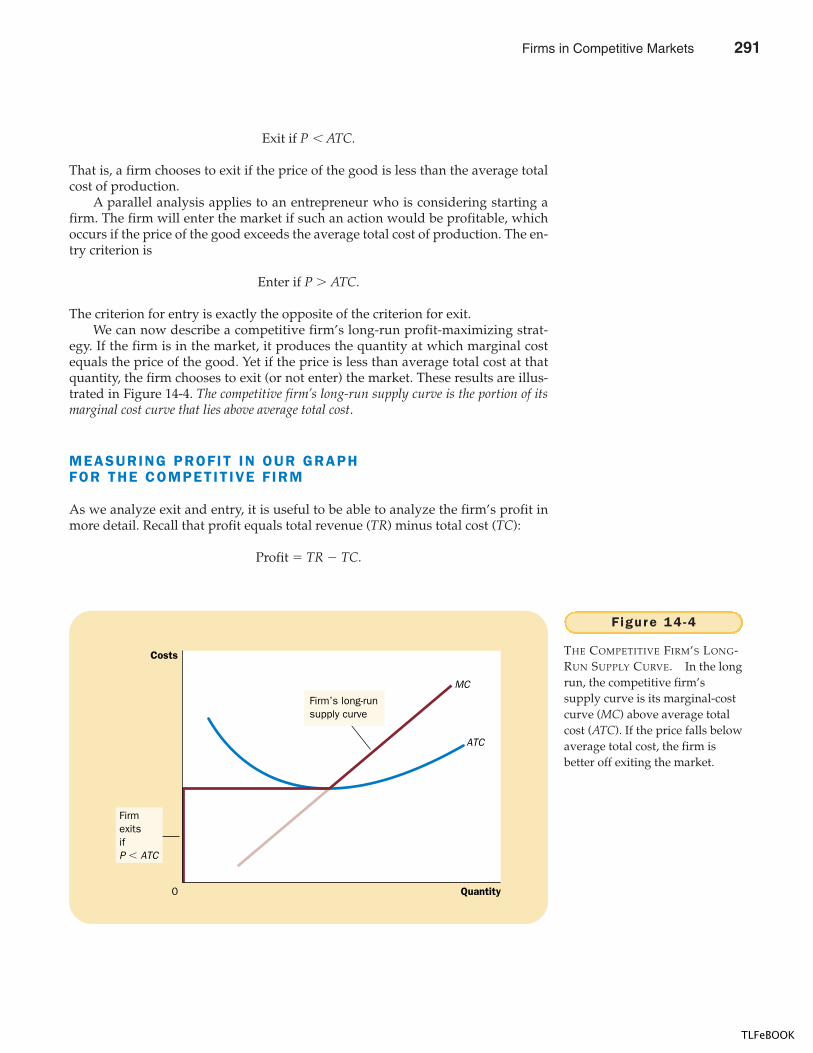
CHAPTER 14 FIRMS IN COMPETIT IVE MARKETS 301
Exit if P � ATC.
That is, a firm chooses to exit if the price of the good is less than the average totalcost of production.
A parallel analysis applies to an entrepreneur who is considering starting afirm. The firm will enter the market if such an action would be profitable, whichoccurs if the price of the good exceeds the average total cost of production. The en-try criterion is
Enter if P � ATC.
The criterion for entry is exactly the opposite of the criterion for exit.We can now describe a competitive firm’s long-run profit-maximizing strat-
egy. If the firm is in the market, it produces the quantity at which marginal costequals the price of the good. Yet if the price is less than average total cost at thatquantity, the firm chooses to exit (or not enter) the market. These results are illus-trated in Figure 14-4. The competitive firm’s long-run supply curve is the portion of itsmarginal cost curve that lies above average total cost.
MEASURING PROFIT IN OUR GRAPHFOR THE COMPETIT IVE F IRM
As we analyze exit and entry, it is useful to be able to analyze the firm’s profit inmore detail. Recall that profit equals total revenue (TR) minus total cost (TC):
Profit � TR � TC.
FirmexitsifP � ATC
Quantity
MC
ATC
0
Costs
Firm’s long-runsupply curve
Figure 14 -4
THE COMPETITIVE FIRM’S LONG-RUN SUPPLY CURVE. In the longrun, the competitive firm’ssupply curve is its marginal-costcurve (MC) above average totalcost (ATC). If the price falls belowaverage total cost, the firm isbetter off exiting the market.
Firms in Competitive Markets 291
TLFeBOOK
302 PART F IVE FIRM BEHAVIOR AND THE ORGANIZATION OF INDUSTRY
We can rewrite this definition by multiplying and dividing the right-hand sideby Q:
Profit � (TR/Q � TC/Q) � Q.
But note that TR/Q is average revenue, which is the price P, and TC/Q is averagetotal cost ATC. Therefore,
Profit � (P � ATC) � Q.
This way of expressing the firm’s profit allows us to measure profit in our graphs.Panel (a) of Figure 14-5 shows a firm earning positive profit. As we have al-
ready discussed, the firm maximizes profit by producing the quantity at whichprice equals marginal cost. Now look at the shaded rectangle. The height of therectangle is P � ATC, the difference between price and average total cost. The
IN THE 1990S, MANY COUNTRIES THAT HAD
previously relied on communist theo-ries of central planning tried to makethe transition to free-market capitalism.According to this article, Poland suc-ceeded because it encouraged free en-try and exit, and Russia failed becauseit didn’t.
R u s s i a I s N o t P o l a n d ,a n d T h a t ’s To o B a d
BY MICHAEL M. WEINSTEIN
Put aside for a moment the frighteningcrash of the ruble and the collapse of
Russia’s stock and bond markets lastweek. They are symptoms of somethinglarger—a deformed economy in whichthe Government sets business taxesthat few firms ever pay, enterprisespromise wages that employees neversee, loans go unpaid, people barter withpots, pans and socks, and shady dealingruns rampant.
It didn’t have to be this way. TheRussians need only look to Poland to be-hold the better road untraveled. Polandtoo began the decade saddled with pal-try living standards bequeathed by asclerotic, centrally controlled economyrun by discredited Communists. Itreached out to the West for help creat-ing monetary, budget, trade and legalregimes, and unlike Russia it followedthrough with sustained political will. Itnow ranks among Europe’s fastest-growing economies.
Key to Poland’s steady suc-cess have been two policy decisions,and discussing them helps to illuminateby contrast what is going wrong withRussia.
First, Poland adopted what might becalled the Balcerowicz rule, named afterLeszek Balcerowicz, the Finance Minis-ter who masterminded Poland’s marketreforms. Mr. Balcerowicz invited thou-sands of would-be entrepreneurs to sell,within loose limits, anything they wantedanywhere they wanted at whateverprice they wanted. Economists calledthis liberalization. The Poles called itcompetition.
The Balcerowicz rule helped breakthe chokehold of Communist-dominated,state-owned enterprises and Govern-ment bureaucracies over economic ac-tivity. Also, encouraging small start-upsdenies organized crime opportunities forlarge prey.
When Poland broke away fromcommunism, Western economists hadwrung their hands trying to figure outwhat to do with its sprawling state-owned factories, which operated morelike social welfare agencies than produc-tion units. The solution, it turned out,was benign neglect. Rather than convertfactories, the Poles allowed them to
IN THE NEWS
Entry and Exit inTransition Economies
292 Firms in Competitive Markets
TLFeBOOK
CHAPTER 14 FIRMS IN COMPETIT IVE MARKETS 303
width of the rectangle is Q, the quantity produced. Therefore, the area of the rec-tangle is (P � ATC) � Q, which is the firm’s profit.
Similarly, panel (b) of this figure shows a firm with losses (negative profit). Inthis case, maximizing profit means minimizing losses, a task accomplished onceagain by producing the quantity at which price equals marginal cost. Now con-sider the shaded rectangle. The height of the rectangle is ATC � P, and the widthis Q. The area is (ATC � P) � Q, which is the firm’s loss. Because a firm in this sit-uation is not making enough revenue to cover its average total cost, the firmwould choose to exit the market.
QUICK QUIZ: How does the price faced by a profit-maximizing competitive firm compare to its marginal cost? Explain. � When does a profit-maximizing competitive firm decide to shut down?
shrivel. Workers peeled away to set upretail shops and other small enterpriseslargely free of Government interference.
The second major decision wasscarier. Poland forced insolvent firmsinto bankruptcy, preventing them fromdraining resources from productive partsof the economy. That also ended a drainon the Federal budget by firms that hadto be propped up by one disguised sub-sidy or another.
There were moments when thepost-Communist Government in Russiaappeared headed in the same direction.In early 1992, the Yeltsin Governmentembraced the Balcerowicz rule. Rus-sians were invited to take to the streetsand set up kiosks and curbside tables,selling whatever they wanted at what-ever price consumers would pay. Butthen Communist antibodies, in the formof the oligarchs who controlled the state-owned factories and natural resources,were activated. They detected foreigntissue and attacked. Local governmentburied the Balcerowicz rule, imposing li-censing and other requirements and
eventually strangling start-ups. ProfessorMarshall Goldman of Harvard points torevealing comments by Viktor S. Cher-nomyrdin, the off-again, on-again PrimeMinister whom President Boris N.Yeltsin restored to his post last week.Mr. Chernomyrdin observed that streetvendors were an unattractive, chaoticblight on a proud country. The Russianauthorities cracked down.
The impact was severe. AndersAslund, a former adviser to the RussianGovernment now at the Carnegie En-dowment for International Peace, esti-mates that since the middle of 1994, thenumber of enterprises in Russia hasstagnated. In a typical Western econ-omy, he estimates, there is 1 businessfor every 10 residents. In Russia, theratio is 1 for every 55.
By snuffing out start-ups, Russialost the remarkable device by whichPoland drained workers out of worthlessfactories into units that could producethe goods that people wanted to buy.
Russia not only stifles start-ups; italso props up incompetents. It tolerates
businesses that cannot pay taxes orwages. They survive because of sys-tems of barter and mutual forbearance ofloans and taxes. Suppliers engage inround-robin lending by which everyoneowes money to someone and no oneever pays up. That too throws a lifelineto insolvent firms.
Russian factories continue to churnout steel and other products that no oneneeds. One measure of the deformity isthat Russia is littered with factories em-ploying 10,000 or more workers. In theUnited States, such factories are a rarity.The effect is to keep alive concerns thatchew up $1.50 worth of resources in or-der to turn out a product that is worthonly $1 to consumers. Economists callthis “negative value added.” Ordinaryfolk call it economic suicide.
SOURCE: The New York Times, August 30, 1998,Week in Review, p. 5.
Firms in Competitive Markets 293
TLFeBOOK
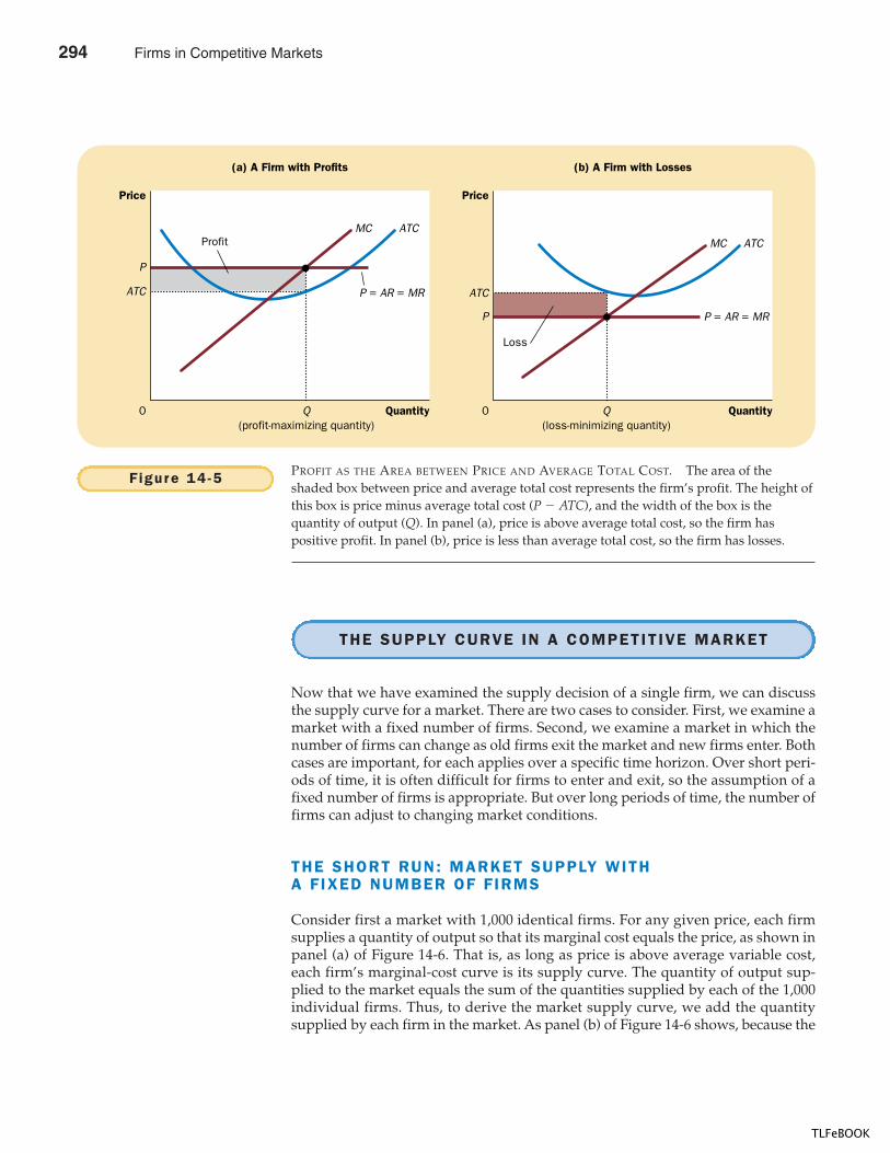
304 PART F IVE FIRM BEHAVIOR AND THE ORGANIZATION OF INDUSTRY
THE SUPPLY CURVE IN A COMPETIT IVE MARKET
Now that we have examined the supply decision of a single firm, we can discussthe supply curve for a market. There are two cases to consider. First, we examine amarket with a fixed number of firms. Second, we examine a market in which thenumber of firms can change as old firms exit the market and new firms enter. Bothcases are important, for each applies over a specific time horizon. Over short peri-ods of time, it is often difficult for firms to enter and exit, so the assumption of afixed number of firms is appropriate. But over long periods of time, the number offirms can adjust to changing market conditions.
THE SHORT RUN: MARKET SUPPLY WITHA FIXED NUMBER OF F IRMS
Consider first a market with 1,000 identical firms. For any given price, each firmsupplies a quantity of output so that its marginal cost equals the price, as shown inpanel (a) of Figure 14-6. That is, as long as price is above average variable cost,each firm’s marginal-cost curve is its supply curve. The quantity of output sup-plied to the market equals the sum of the quantities supplied by each of the 1,000individual firms. Thus, to derive the market supply curve, we add the quantitysupplied by each firm in the market. As panel (b) of Figure 14-6 shows, because the
(a) A Firm with Profits (b) A Firm with Losses
Quantity0
Price
Quantity0
Price
P = AR = MR
ProfitATCMC
P
ATC ATC
Q(profit-maximizing quantity)
P = AR = MR
Loss
ATCMC
Q(loss-minimizing quantity)
P
Figure 14 -5 PROFIT AS THE AREA BETWEEN PRICE AND AVERAGE TOTAL COST. The area of theshaded box between price and average total cost represents the firm’s profit. The height ofthis box is price minus average total cost (P � ATC), and the width of the box is thequantity of output (Q). In panel (a), price is above average total cost, so the firm haspositive profit. In panel (b), price is less than average total cost, so the firm has losses.
294 Firms in Competitive Markets
TLFeBOOK
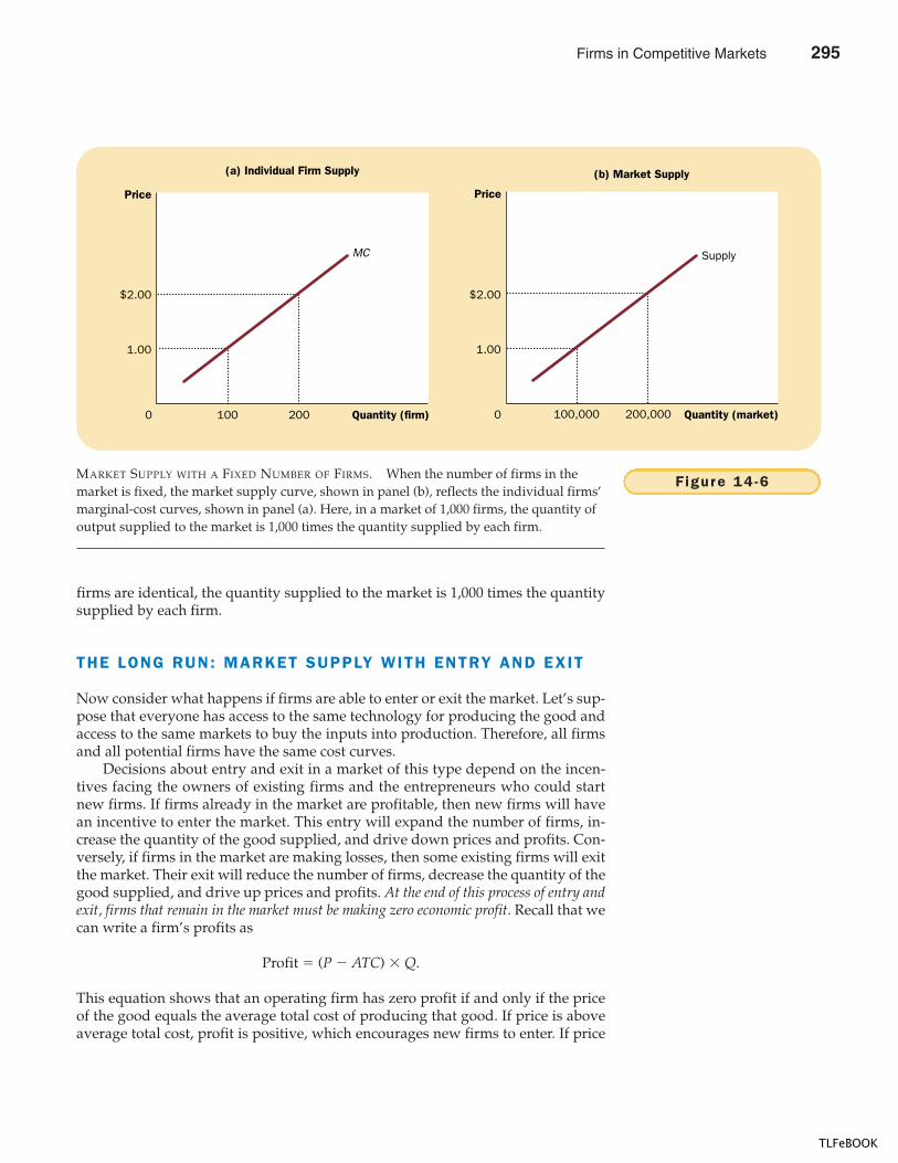
CHAPTER 14 FIRMS IN COMPETIT IVE MARKETS 305
firms are identical, the quantity supplied to the market is 1,000 times the quantitysupplied by each firm.
THE LONG RUN: MARKET SUPPLY WITH ENTRY AND EXIT
Now consider what happens if firms are able to enter or exit the market. Let’s sup-pose that everyone has access to the same technology for producing the good andaccess to the same markets to buy the inputs into production. Therefore, all firmsand all potential firms have the same cost curves.
Decisions about entry and exit in a market of this type depend on the incen-tives facing the owners of existing firms and the entrepreneurs who could startnew firms. If firms already in the market are profitable, then new firms will havean incentive to enter the market. This entry will expand the number of firms, in-crease the quantity of the good supplied, and drive down prices and profits. Con-versely, if firms in the market are making losses, then some existing firms will exitthe market. Their exit will reduce the number of firms, decrease the quantity of thegood supplied, and drive up prices and profits. At the end of this process of entry andexit, firms that remain in the market must be making zero economic profit. Recall that wecan write a firm’s profits as
Profit � (P � ATC) � Q.
This equation shows that an operating firm has zero profit if and only if the priceof the good equals the average total cost of producing that good. If price is aboveaverage total cost, profit is positive, which encourages new firms to enter. If price
(a) Individual Firm Supply
Quantity (firm)0
Price
MC
$2.00
1.00
100 200
(b) Market Supply
Quantity (market)0
Price
Supply
$2.00
1.00
100,000 200,000
Figure 14 -6MARKET SUPPLY WITH A FIXED NUMBER OF FIRMS. When the number of firms in themarket is fixed, the market supply curve, shown in panel (b), reflects the individual firms’marginal-cost curves, shown in panel (a). Here, in a market of 1,000 firms, the quantity ofoutput supplied to the market is 1,000 times the quantity supplied by each firm.
Firms in Competitive Markets 295
TLFeBOOK
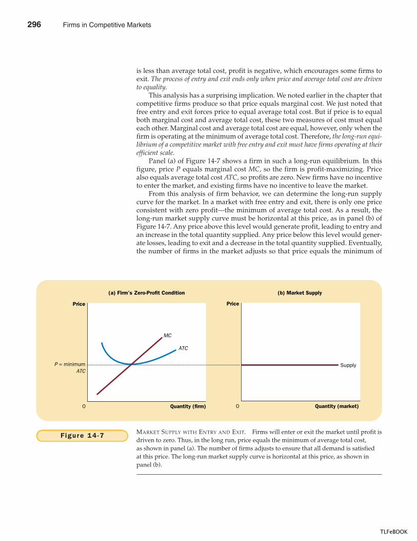
306 PART F IVE FIRM BEHAVIOR AND THE ORGANIZATION OF INDUSTRY
is less than average total cost, profit is negative, which encourages some firms toexit. The process of entry and exit ends only when price and average total cost are drivento equality.
This analysis has a surprising implication. We noted earlier in the chapter thatcompetitive firms produce so that price equals marginal cost. We just noted thatfree entry and exit forces price to equal average total cost. But if price is to equalboth marginal cost and average total cost, these two measures of cost must equaleach other. Marginal cost and average total cost are equal, however, only when thefirm is operating at the minimum of average total cost. Therefore, the long-run equi-librium of a competitive market with free entry and exit must have firms operating at theirefficient scale.
Panel (a) of Figure 14-7 shows a firm in such a long-run equilibrium. In thisfigure, price P equals marginal cost MC, so the firm is profit-maximizing. Pricealso equals average total cost ATC, so profits are zero. New firms have no incentiveto enter the market, and existing firms have no incentive to leave the market.
From this analysis of firm behavior, we can determine the long-run supplycurve for the market. In a market with free entry and exit, there is only one priceconsistent with zero profit—the minimum of average total cost. As a result, thelong-run market supply curve must be horizontal at this price, as in panel (b) ofFigure 14-7. Any price above this level would generate profit, leading to entry andan increase in the total quantity supplied. Any price below this level would gener-ate losses, leading to exit and a decrease in the total quantity supplied. Eventually,the number of firms in the market adjusts so that price equals the minimum of
(a) Firm’s Zero-Profit Condition
Quantity (firm)0
Price
P = minimumATC
(b) Market Supply
Quantity (market)
Price
0
Supply
MC
ATC
Figure 14 -7 MARKET SUPPLY WITH ENTRY AND EXIT. Firms will enter or exit the market until profit isdriven to zero. Thus, in the long run, price equals the minimum of average total cost,as shown in panel (a). The number of firms adjusts to ensure that all demand is satisfiedat this price. The long-run market supply curve is horizontal at this price, as shown inpanel (b).
296 Firms in Competitive Markets
TLFeBOOK
CHAPTER 14 FIRMS IN COMPETIT IVE MARKETS 307
average total cost, and there are enough firms to satisfy all the demand at thisprice.
WHY DO COMPETIT IVE F IRMS STAY IN BUSINESSIF THEY MAKE ZERO PROFIT?
At first, it might seem odd that competitive firms earn zero profit in the long run.After all, people start businesses to make a profit. If entry eventually drives profitto zero, there might seem to be little reason to stay in business.
To understand the zero-profit condition more fully, recall that profit equals to-tal revenue minus total cost, and that total cost includes all the opportunity costsof the firm. In particular, total cost includes the opportunity cost of the time andmoney that the firm owners devote to the business. In the zero-profit equilibrium,the firm’s revenue must compensate the owners for the time and money that theyexpend to keep their business going.
Consider an example. Suppose that a farmer had to invest $1 million to openhis farm, which otherwise he could have deposited in a bank to earn $50,000 a yearin interest. In addition, he had to give up another job that would have paid him$30,000 a year. Then the farmer’s opportunity cost of farming includes both the in-terest he could have earned and the forgone wages—a total of $80,000. Even if hisprofit is driven to zero, his revenue from farming compensates him for these op-portunity costs.
Keep in mind that accountants and economists measure costs differently. Aswe discussed in Chapter 13, accountants keep track of explicit costs but usuallymiss implicit costs. That is, they measure costs that require an outflow of moneyfrom the firm, but they fail to include opportunity costs of production that do notinvolve an outflow of money. As a result, in the zero-profit equilibrium, economicprofit is zero, but accounting profit is positive. Our farmer’s accountant, for in-stance, would conclude that the farmer earned an accounting profit of $80,000,which is enough to keep the farmer in business.
“We’re a nonprofit organization—we don’t intend to be, but we are!”
Firms in Competitive Markets 297
TLFeBOOK
308 PART F IVE FIRM BEHAVIOR AND THE ORGANIZATION OF INDUSTRY
A SHIFT IN DEMAND IN THE SHORT RUN AND LONG RUN
Because firms can enter and exit a market in the long run but not in the short run,the response of a market to a change in demand depends on the time horizon. Tosee this, let’s trace the effects of a shift in demand. This analysis will show how amarket responds over time, and it will show how entry and exit drive a market toits long-run equilibrium.
Suppose the market for milk begins in long-run equilibrium. Firms are earn-ing zero profit, so price equals the minimum of average total cost. Panel (a) of Fig-ure 14-8 shows the situation. The long-run equilibrium is point A, the quantitysold in the market is Q1, and the price is P1.
Now suppose scientists discover that milk has miraculous health benefits. Asa result, the demand curve for milk shifts outward from D1 to D2, as in panel (b).The short-run equilibrium moves from point A to point B; as a result, the quantityrises from Q1 to Q2, and the price rises from P1 to P2. All of the existing firms re-spond to the higher price by raising the amount produced. Because each firm’ssupply curve reflects its marginal-cost curve, how much they each increase pro-duction is determined by the marginal-cost curve. In the new, short-run equilib-rium, the price of milk exceeds average total cost, so the firms are making positiveprofit.
Over time, the profit in this market encourages new firms to enter. Some farm-ers may switch to milk from other farm products, for example. As the number offirms grows, the short-run supply curve shifts to the right from S1 to S2, as in panel(c), and this shift causes the price of milk to fall. Eventually, the price is driven backdown to the minimum of average total cost, profits are zero, and firms stop enter-ing. Thus, the market reaches a new long-run equilibrium, point C. The price ofmilk has returned to P1, but the quantity produced has risen to Q3. Each firm isagain producing at its efficient scale, but because more firms are in the dairy busi-ness, the quantity of milk produced and sold is higher.
WHY THE LONG-RUN SUPPLY CURVEMIGHT SLOPE UPWARD
So far we have seen that entry and exit can cause the long-run market supplycurve to be horizontal. The essence of our analysis is that there are a large numberof potential entrants, each of which faces the same costs. As a result, the long-runmarket supply curve is horizontal at the minimum of average total cost. When thedemand for the good increases, the long-run result is an increase in the number offirms and in the total quantity supplied, without any change in the price.
There are, however, two reasons that the long-run market supply curve mightslope upward. The first is that some resource used in production may be availableonly in limited quantities. For example, consider the market for farm products.Anyone can choose to buy land and start a farm, but the quantity of land is lim-ited. As more people become farmers, the price of farmland is bid up, which raisesthe costs of all farmers in the market. Thus, an increase in demand for farm prod-ucts cannot induce an increase in quantity supplied without also inducing a rise infarmers’ costs, which in turn means a rise in price. The result is a long-run marketsupply curve that is upward sloping, even with free entry into farming.
A second reason for an upward-sloping supply curve is that firms may havedifferent costs. For example, consider the market for painters. Anyone can enter
298 Firms in Competitive Markets
TLFeBOOK
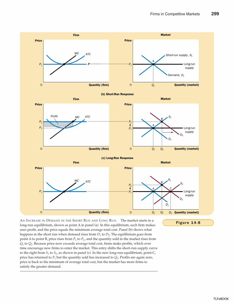
Firm
(a) Initial Condition
Quantity (firm)0
Price
Market
Market
Quantity (market)
Long-runsupply
Price
0
Demand, D1
Short-run supply, S1
Firm
(b) Short-Run Response
Quantity (firm)0
Price
P1 P
MC ATC
MC ATC
P1P
Profit
P1
P1
P2
Firm(c) Long-Run Response
Quantity (firm)0
Price
MC ATC
A
Quantity (market)
Long-runsupply
Price
0
D1
D2
P1
Q1
Q1
Q2
P2
A
B
Market
Quantity (market)
Price
0
P1
P2
Q1 Q2
Long-runsupply
Q3
C
B
D1
D2
S1
S1
A
S2
Figure 14 -8AN INCREASE IN DEMAND IN THE SHORT RUN AND LONG RUN. The market starts in along-run equilibrium, shown as point A in panel (a). In this equilibrium, each firm makeszero profit, and the price equals the minimum average total cost. Panel (b) shows whathappens in the short run when demand rises from D1 to D2. The equilibrium goes frompoint A to point B, price rises from P1 to P2, and the quantity sold in the market rises fromQ1 to Q2. Because price now exceeds average total cost, firms make profits, which overtime encourage new firms to enter the market. This entry shifts the short-run supply curveto the right from S1 to S2, as shown in panel (c). In the new long-run equilibrium, point C,price has returned to P1 but the quantity sold has increased to Q3. Profits are again zero,price is back to the minimum of average total cost, but the market has more firms tosatisfy the greater demand.
Firms in Competitive Markets 299
TLFeBOOK
310 PART F IVE FIRM BEHAVIOR AND THE ORGANIZATION OF INDUSTRY
the market for painting services, but not everyone has the same costs. Costs varyin part because some people work faster than others and in part because somepeople have better alternative uses of their time than others. For any given price,those with lower costs are more likely to enter than those with higher costs. To in-crease the quantity of painting services supplied, additional entrants must be en-couraged to enter the market. Because these new entrants have higher costs, theprice must rise to make entry profitable for them. Thus, the market supply curvefor painting services slopes upward even with free entry into the market.
Notice that if firms have different costs, some firms earn profit even in the longrun. In this case, the price in the market reflects the average total cost of the mar-ginal firm—the firm that would exit the market if the price were any lower. Thisfirm earns zero profit, but firms with lower costs earn positive profit. Entry doesnot eliminate this profit because would-be entrants have higher costs than firms al-ready in the market. Higher-cost firms will enter only if the price rises, making themarket profitable for them.
IN COMPETITIVE MARKETS, STRONG DE-mand leads to high prices and highprofits, which then lead to increasedentry, falling prices, and falling profits.To economists, these market forcesare one reflection of the invisible handat work. To the business managers,however, new entry and fallingprofits can seem like a “problem ofoverinvestment.”
I n S o m e I n d u s t r i e s , E x e c u t i v e sF o r e s e e To u g h Ti m e s A h e a d ;A K e y C u l p r i t : H i g h P r o f i t s
BY BERNARD WYSOCKI, JR.MONTEREY, CALIF.—About 20 execu-tives are huddled in a conference room
with a team of management consultants,and the mood is surprisingly somber.
It’s a fine summer day, the stockmarket is booming, the U.S. economy isin great shape, and some of the com-panies represented here are postingstronger-than-expected profits. Best ofall, perhaps, these lucky executives arejust a chip shot away from the famedPebble Beach golf course. They ought tobe euphoric.
Instead, an undertone of concern isevident among these executives fromMobil Corp., Union Carbide Corp. andother capital-intensive companies. In be-tween golf, fine meals and cigars, theyhear a sobering message from theirhosts.
“I feel like the prophet of doom” isthe welcoming line of R. Duane Dickson,a director of Mercer Management Con-sulting and host of the meeting. “It’s ourbelief that the downturn has started. Ican’t tell you how far it’s going to go. Butit could be a very ugly one.”
For two days, the executives andtheir advisers discuss what they expectin their industries between now and2000: growing overcapacity, world-wide
product gluts, price wars, shakeouts,and consolidations. . . .
One man who attended the PebbleBeach meeting, Joseph Soviero, a UnionCarbide vice president, cites an odd butbasic problem in chemicals: the strongprofits of the past few years. “The prof-itability that the industry sees during thegood times has always led to overinvest-ing, and it has this time,” Mr. Sovierosays. He adds that the chemicals busi-ness cycle is alive and has peaked. AtUnion Carbide, he says, “we always talkabout the cycle” and try to manage it.
So far, demand isn’t a big problem.In many industries, it is still growingsteadily, though slowly. What is develop-ing is too much supply, stemming fromthe recurring problem of overinvestment.. . . The next few years will bring fiercecompetition and falling prices.
SOURCE: The Wall Street Journal, August 7, 1997,p. A1.
IN THE NEWS
Entry or Overinvestment?
300 Firms in Competitive Markets
TLFeBOOK
CHAPTER 14 FIRMS IN COMPETIT IVE MARKETS 311
Thus, for these two reasons, the long-run supply curve in a market may be up-ward sloping rather than horizontal, indicating that a higher price is necessary toinduce a larger quantity supplied. Nonetheless, the basic lesson about entry andexit remains true. Because firms can enter and exit more easily in the long run than in theshort run, the long-run supply curve is typically more elastic than the short-run supplycurve.
QUICK QUIZ: In the long run with free entry and exit, is the price in a market equal to marginal cost, average total cost, both, or neither? Explain with a diagram.
CONCLUSION: BEHIND THE SUPPLY CURVE
We have been discussing the behavior of competitive profit-maximizing firms. Youmay recall from Chapter 1 that one of the Ten Principles of Economics is that rationalpeople think at the margin. This chapter has applied this idea to the competitivefirm. Marginal analysis has given us a theory of the supply curve in a competitivemarket and, as a result, a deeper understanding of market outcomes.
We have learned that when you buy a good from a firm in a competitive mar-ket, you can be assured that the price you pay is close to the cost of producing thatgood. In particular, if firms are competitive and profit-maximizing, the price of agood equals the marginal cost of making that good. In addition, if firms can freelyenter and exit the market, the price also equals the lowest possible average totalcost of production.
Although we have assumed throughout this chapter that firms are price tak-ers, many of the tools developed here are also useful for studying firms in lesscompetitive markets. In the next three chapters we will examine the behavior offirms with market power. Marginal analysis will again be useful in analyzing thesefirms, but it will have quite different implications.
� Because a competitive firm is a price taker, its revenue isproportional to the amount of output it produces. Theprice of the good equals both the firm’s average revenueand its marginal revenue.
� To maximize profit, a firm chooses a quantity of outputsuch that marginal revenue equals marginal cost.Because marginal revenue for a competitive firm equalsthe market price, the firm chooses quantity so that priceequals marginal cost. Thus, the firm’s marginal costcurve is its supply curve.
� In the short run when a firm cannot recover its fixedcosts, the firm will choose to shut down temporarily if
the price of the good is less than average variable cost.In the long run when the firm can recover both fixedand variable costs, it will choose to exit if the price isless than average total cost.
� In a market with free entry and exit, profits are driven tozero in the long run. In this long-run equilibrium, allfirms produce at the efficient scale, price equals theminimum of average total cost, and the number of firmsadjusts to satisfy the quantity demanded at this price.
� Changes in demand have different effects over differenttime horizons. In the short run, an increase in demandraises prices and leads to profits, and a decrease in
Summar y
Firms in Competitive Markets 301
TLFeBOOK
312 PART F IVE FIRM BEHAVIOR AND THE ORGANIZATION OF INDUSTRY
demand lowers prices and leads to losses. But if firmscan freely enter and exit the market, then in the long run
the number of firms adjusts to drive the market back tothe zero-profit equilibrium.
competitive market, p. 292average revenue, p. 294
marginal revenue, p. 294 sunk cost, p. 298
Key Concepts
1. What is meant by a competitive firm?
2. Draw the cost curves for a typical firm. For a givenprice, explain how the firm chooses the level of outputthat maximizes profit.
3. Under what conditions will a firm shut downtemporarily? Explain.
4. Under what conditions will a firm exit a market?Explain.
5. Does a firm’s price equal marginal cost in the short run,in the long run, or both? Explain.
6. Does a firm’s price equal the minimum of average totalcost in the short run, in the long run, or both? Explain.
7. Are market supply curves typically more elastic in theshort run or in the long run? Explain.
Quest ions fo r Rev iew
1. What are the characteristics of a competitive market?Which of the following drinks do you think is bestdescribed by these characteristics? Why aren’t theothers?a. tap waterb. bottled waterc. colad. beer
2. Your roommate’s long hours in Chem lab finally paidoff—she discovered a secret formula that lets people doan hour’s worth of studying in 5 minutes. So far, she’ssold 200 doses, and faces the following average-total-cost schedule:
Q AVERAGE TOTAL COST
199 $199200 200201 201
If a new customer offers to pay your roommate $300 forone dose, should she make one more? Explain.
3. The licorice industry is competitive. Each firm produces2 million strings of licorice per year. The strings have anaverage total cost of $0.20 each, and they sell for $0.30.a. What is the marginal cost of a string?
b. Is this industry in long-run equilibrium? Why orwhy not?
4. You go out to the best restaurant in town and order alobster dinner for $40. After eating half of the lobster,you realize that you are quite full. Your date wants youto finish your dinner, because you can’t take it homeand because “you’ve already paid for it.” What shouldyou do? Relate your answer to the material in thischapter.
5. Bob’s lawn-mowing service is a profit-maximizing,competitive firm. Bob mows lawns for $27 each. Histotal cost each day is $280, of which $30 is a fixed cost.He mows 10 lawns a day. What can you say about Bob’sshort-run decision regarding shut down and his long-run decision regarding exit?
6. Consider total cost and total revenue given in the tablebelow:
QUANTITY
0 1 2 3 4 5 6 7
Total cost $8 $9 $10 $11 $13 $19 $27 $37Total revenue 0 8 16 24 32 40 48 56
a. Calculate profit for each quantity. How muchshould the firm produce to maximize profit?
Prob lems and App l icat ions
302 Firms in Competitive Markets
TLFeBOOK
CHAPTER 14 FIRMS IN COMPETIT IVE MARKETS 313
b. Calculate marginal revenue and marginal cost foreach quantity. Graph them. (Hint: Put the pointsbetween whole numbers. For example, the marginalcost between 2 and 3 should be graphed at 2 1/2.)At what quantity do these curves cross? How doesthis relate to your answer to part (a)?
c. Can you tell whether this firm is in a competitiveindustry? If so, can you tell whether the industry isin a long-run equilibrium?
7. From The Wall Street Journal (July 23, 1991): “Sincepeaking in 1976, per capita beef consumption in theUnited States has fallen by 28.6 percent . . . [and] the sizeof the U.S. cattle herd has shrunk to a 30-year low.”a. Using firm and industry diagrams, show the short-
run effect of declining demand for beef. Label thediagram carefully and write out in words all of thechanges you can identify.
b. On a new diagram, show the long-run effect ofdeclining demand for beef. Explain in words.
8. “High prices traditionally cause expansion in anindustry, eventually bringing an end to high prices andmanufacturers’ prosperity.” Explain, using appropriatediagrams.
9. Suppose the book-printing industry is competitive andbegins in a long-run equilibrium.a. Draw a diagram describing the typical firm in the
industry.b. Hi-Tech Printing Company invents a new process
that sharply reduces the cost of printing books.What happens to Hi-Tech’s profits and the price ofbooks in the short run when Hi-Tech’s patentprevents other firms from using the newtechnology?
c. What happens in the long run when the patentexpires and other firms are free to use thetechnology?
10. Many small boats are made of fiberglass, which isderived from crude oil. Suppose that the price of oilrises.a. Using diagrams, show what happens to the cost
curves of an individual boat-making firm and to themarket supply curve.
b. What happens to the profits of boat makers in theshort run? What happens to the number of boatmakers in the long run?
11. Suppose that the U.S. textile industry is competitive,and there is no international trade in textiles. In long-run equilibrium, the price per unit of cloth is $30.a. Describe the equilibrium using graphs for the entire
market and for an individual producer.
Now suppose that textile producers in other countriesare willing to sell large quantities of cloth in the UnitedStates for only $25 per unit.b. Assuming that U.S. textile producers have large
fixed costs, what is the short-run effect of theseimports on the quantity produced by an individualproducer? What is the short-run effect on profits?Illustrate your answer with a graph.
c. What is the long-run effect on the number of U.S.firms in the industry?
12. Suppose there are 1,000 hot pretzel stands operating inNew York City. Each stand has the usual U-shapedaverage-total-cost curve. The market demand curve forpretzels slopes downward, and the market for pretzelsis in long-run competitive equilibrium.a. Draw the current equilibrium, using graphs for the
entire market and for an individual pretzel stand.b. Now the city decides to restrict the number of
pretzel-stand licenses, reducing the number ofstands to only 800. What effect will this action haveon the market and on an individual stand that isstill operating? Use graphs to illustrate youranswer.
c. Suppose that the city decides to charge a license feefor the 800 licenses. How will this affect the numberof pretzels sold by an individual stand, and thestand’s profit? The city wants to raise as muchrevenue as possible and also wants to ensure that800 pretzel stands remain in the city. By how muchshould the city increase the license fee? Show theanswer on your graph.
13. Assume that the gold-mining industry is competitive.a. Illustrate a long-run equilibrium using diagrams for
the gold market and for a representative gold mine.b. Suppose that an increase in jewelry demand
induces a surge in the demand for gold. Using yourdiagrams, show what happens in the short run tothe gold market and to each existing gold mine.
c. If the demand for gold remains high, what wouldhappen to the price over time? Specifically, wouldthe new long-run equilibrium price be above,below, or equal to the short-run equilibrium price inpart (b)? Is it possible for the new long-runequilibrium price to be above the original long-runequilibrium price? Explain.
14. (This problem is challenging.) The New York Times(July 1, 1994) reported on a Clinton administrationproposal to lift the ban on exporting oil from theNorth Slope of Alaska. According to the article, theadministration said that “the chief effect of the ban has
Firms in Competitive Markets 303
TLFeBOOK
314 PART F IVE FIRM BEHAVIOR AND THE ORGANIZATION OF INDUSTRY
been to provide California refiners with crude oilcheaper than oil on the world market. . . . The bancreated a subsidy for California refiners that had notbeen passed on to consumers.” Let’s use our analysis offirm behavior to analyze these claims.a. Draw the cost curves for a California refiner and for
a refiner in another part of the world. Assume thatthe California refiners have access to inexpensiveAlaskan crude oil and that other refiners must buymore expensive crude oil from the Middle East.
b. All of the refiners produce gasoline for the worldgasoline market, which has a single price. In thelong-run equilibrium, will this price depend on thecosts faced by California producers or the costsfaced by other producers? Explain. (Hint: Californiacannot itself supply the entire world market.) Drawnew graphs that illustrate the profits earned by aCalifornia refiner and another refiner.
c. In this model, is there a subsidy to Californiarefiners? Is it passed on to consumers?
304 Firms in Competitive Markets
TLFeBOOK
315
IN THIS CHAPTERYOU WILL . . .
See why monopol iest r y to charge
d i f fe rent p r ices tod i f fe rent customers
See how themonopoly ’s
dec is ions a f fecteconomic wel l -be ing
Learn why somemarkets have on ly
one se l le r
Ana lyze how amonopoly
determines thequant i ty to produce
and the pr ice tocharge
Cons ider thevar ious pub l ic
po l ic ies a imed atso lv ing the prob lem
of monopoly
If you own a personal computer, it probably uses some version of Windows, theoperating system sold by the Microsoft Corporation. When Microsoft first de-signed Windows many years ago, it applied for and received a copyright from thegovernment. The copyright gives Microsoft the exclusive right to make and sellcopies of the Windows operating system. So if a person wants to buy a copy ofWindows, he or she has little choice but to give Microsoft the approximately $50that the firm has decided to charge for its product. Microsoft is said to have a mo-nopoly in the market for Windows.
Microsoft’s business decisions are not well described by the model of firmbehavior we developed in Chapter 14. In that chapter, we analyzed competitive mar-kets, in which there are many firms offering essentially identical products, so eachfirm has little influence over the price it receives. By contrast, a monopoly such asMicrosoft has no close competitors and, therefore, can influence the market price ofits product. While a competitive firm is a price taker, a monopoly firm is a price maker.
M O N O P O L Y
305
15
TLFeBOOK
316 PART F IVE FIRM BEHAVIOR AND THE ORGANIZATION OF INDUSTRY
In this chapter we examine the implications of this market power. We will seethat market power alters the relationship between a firm’s price and its costs. Acompetitive firm takes the price of its output as given by the market and thenchooses the quantity it will supply so that price equals marginal cost. By contrast,the price charged by a monopoly exceeds marginal cost. This result is clearly truein the case of Microsoft’s Windows. The marginal cost of Windows—the extra costthat Microsoft would incur by printing one more copy of the program onto somefloppy disks or a CD—is only a few dollars. The market price of Windows is manytimes marginal cost.
It is perhaps not surprising that monopolies charge high prices for their prod-ucts. Customers of monopolies might seem to have little choice but to pay what-ever the monopoly charges. But, if so, why does a copy of Windows not cost $500?Or $5,000? The reason, of course, is that if Microsoft set the price that high, fewerpeople would buy the product. People would buy fewer computers, switch toother operating systems, or make illegal copies. Monopolies cannot achieve anylevel of profit they want, because high prices reduce the amount that their cus-tomers buy. Although monopolies can control the prices of their goods, their prof-its are not unlimited.
As we examine the production and pricing decisions of monopolies, we alsoconsider the implications of monopoly for society as a whole. Monopoly firms, likecompetitive firms, aim to maximize profit. But this goal has very different ramifi-cations for competitive and monopoly firms. As we first saw in Chapter 7, self-interested buyers and sellers in competitive markets are unwittingly led by aninvisible hand to promote general economic well-being. By contrast, becausemonopoly firms are unchecked by competition, the outcome in a market with amonopoly is often not in the best interest of society.
One of the Ten Principles of Economics in Chapter 1 is that governments cansometimes improve market outcomes. The analysis in this chapter will shed morelight on this principle. As we examine the problems that monopolies raise for so-ciety, we will also discuss the various ways in which government policymakersmight respond to these problems. The U.S. government, for example, keeps a closeeye on Microsoft’s business decisions. In 1994, it prevented Microsoft from buyingIntuit, a software firm that sells the leading program for personal finance, on thegrounds that the combination of Microsoft and Intuit would concentrate too muchmarket power in one firm. Similarly, in 1998, the U.S. Justice Department objectedwhen Microsoft started integrating its Internet browser into its Windows operat-ing system, claiming that this would impede competition from other companies,such as Netscape. This concern led the Justice Department to file suit againstMicrosoft, the final resolution of which was still unsettled as this book was goingto press.
WHY MONOPOLIES ARISE
A firm is a monopoly if it is the sole seller of its product and if its product does nothave close substitutes. The fundamental cause of monopoly is barriers to entry: A mo-nopoly remains the only seller in its market because other firms cannot enterthe market and compete with it. Barriers to entry, in turn, have three main sources:
monopolya firm that is the sole seller of aproduct without close substitutes
306 Monopoly
TLFeBOOK
CHAPTER 15 MONOPOLY 317
CASE STUDY THE DEBEERS DIAMOND MONOPOLY
A classic example of a monopoly that arises from the ownership of a key re-source is DeBeers, the South African diamond company. DeBeers controls about80 percent of the world’s production of diamonds. Although the firm’s share ofthe market is not 100 percent, it is large enough to exert substantial influenceover the market price of diamonds.
How much market power does DeBeers have? The answer depends in parton whether there are close substitutes for its product. If people view emeralds,rubies, and sapphires as good substitutes for diamonds, then DeBeers has rela-tively little market power. In this case, any attempt by DeBeers to raise the priceof diamonds would cause people to switch to other gemstones. But if peopleview these other stones as very different from diamonds, then DeBeers can ex-ert substantial influence over the price of its product.
DeBeers pays for large amounts of advertising. At first, this decision mightseem surprising. If a monopoly is the sole seller of its product, why does it needto advertise? One goal of the DeBeers ads is to differentiate diamonds from othergems in the minds of consumers. When their slogan tells you that “a diamondis forever,” you are meant to think that the same is not true of emeralds, rubies,and sapphires. (And notice that the slogan is applied to all diamonds, not justDeBeers diamonds—a sign of DeBeers’s monopoly position.) If the ads are
� A key resource is owned by a single firm.� The government gives a single firm the exclusive right to produce some
good or service.� The costs of production make a single producer more efficient than a large
number of producers.
Let’s briefly discuss each of these.
MONOPOLY RESOURCES
The simplest way for a monopoly to arise is for a single firm to own a key resource.For example, consider the market for water in a small town in the Old West. Ifdozens of town residents have working wells, the competitive model discussed inChapter 14 describes the behavior of sellers. As a result, the price of a gallon of wa-ter is driven to equal the marginal cost of pumping an extra gallon. But if there isonly one well in town and it is impossible to get water from anywhere else, thenthe owner of the well has a monopoly on water. Not surprisingly, the monopolisthas much greater market power than any single firm in a competitive market. Inthe case of a necessity like water, the monopolist could command quite a highprice, even if the marginal cost is low.
Although exclusive ownership of a key resource is a potential cause of mo-nopoly, in practice monopolies rarely arise for this reason. Actual economies arelarge, and resources are owned by many people. Indeed, because many goods aretraded internationally, the natural scope of their markets is often worldwide. Thereare, therefore, few examples of firms that own a resource for which there are noclose substitutes.
“Rather than a monopoly, we liketo consider ourselves ‘the onlygame in town.’”
Monopoly 307
TLFeBOOK
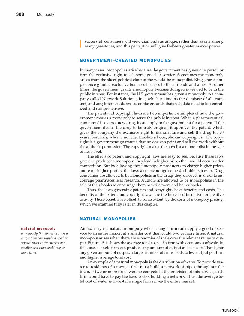
318 PART F IVE FIRM BEHAVIOR AND THE ORGANIZATION OF INDUSTRY
successful, consumers will view diamonds as unique, rather than as one amongmany gemstones, and this perception will give DeBeers greater market power.
GOVERNMENT-CREATED MONOPOLIES
In many cases, monopolies arise because the government has given one person orfirm the exclusive right to sell some good or service. Sometimes the monopolyarises from the sheer political clout of the would-be monopolist. Kings, for exam-ple, once granted exclusive business licenses to their friends and allies. At othertimes, the government grants a monopoly because doing so is viewed to be in thepublic interest. For instance, the U.S. government has given a monopoly to a com-pany called Network Solutions, Inc., which maintains the database of all .com,.net, and .org Internet addresses, on the grounds that such data need to be central-ized and comprehensive.
The patent and copyright laws are two important examples of how the gov-ernment creates a monopoly to serve the public interest. When a pharmaceuticalcompany discovers a new drug, it can apply to the government for a patent. If thegovernment deems the drug to be truly original, it approves the patent, whichgives the company the exclusive right to manufacture and sell the drug for 20years. Similarly, when a novelist finishes a book, she can copyright it. The copy-right is a government guarantee that no one can print and sell the work withoutthe author’s permission. The copyright makes the novelist a monopolist in the saleof her novel.
The effects of patent and copyright laws are easy to see. Because these lawsgive one producer a monopoly, they lead to higher prices than would occur undercompetition. But by allowing these monopoly producers to charge higher pricesand earn higher profits, the laws also encourage some desirable behavior. Drugcompanies are allowed to be monopolists in the drugs they discover in order to en-courage pharmaceutical research. Authors are allowed to be monopolists in thesale of their books to encourage them to write more and better books.
Thus, the laws governing patents and copyrights have benefits and costs. Thebenefits of the patent and copyright laws are the increased incentive for creativeactivity. These benefits are offset, to some extent, by the costs of monopoly pricing,which we examine fully later in this chapter.
NATURAL MONOPOLIES
An industry is a natural monopoly when a single firm can supply a good or ser-vice to an entire market at a smaller cost than could two or more firms. A naturalmonopoly arises when there are economies of scale over the relevant range of out-put. Figure 15-1 shows the average total costs of a firm with economies of scale. Inthis case, a single firm can produce any amount of output at least cost. That is, forany given amount of output, a larger number of firms leads to less output per firmand higher average total cost.
An example of a natural monopoly is the distribution of water. To provide wa-ter to residents of a town, a firm must build a network of pipes throughout thetown. If two or more firms were to compete in the provision of this service, eachfirm would have to pay the fixed cost of building a network. Thus, the average to-tal cost of water is lowest if a single firm serves the entire market.
natura l monopolya monopoly that arises because asingle firm can supply a good orservice to an entire market at asmaller cost than could two ormore firms
308 Monopoly
TLFeBOOK
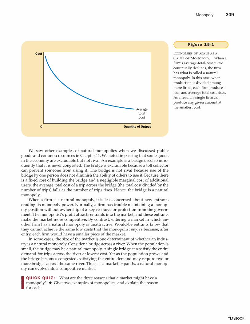
CHAPTER 15 MONOPOLY 319
We saw other examples of natural monopolies when we discussed publicgoods and common resources in Chapter 11. We noted in passing that some goodsin the economy are excludable but not rival. An example is a bridge used so infre-quently that it is never congested. The bridge is excludable because a toll collectorcan prevent someone from using it. The bridge is not rival because use of thebridge by one person does not diminish the ability of others to use it. Because thereis a fixed cost of building the bridge and a negligible marginal cost of additionalusers, the average total cost of a trip across the bridge (the total cost divided by thenumber of trips) falls as the number of trips rises. Hence, the bridge is a naturalmonopoly.
When a firm is a natural monopoly, it is less concerned about new entrantseroding its monopoly power. Normally, a firm has trouble maintaining a monop-oly position without ownership of a key resource or protection from the govern-ment. The monopolist’s profit attracts entrants into the market, and these entrantsmake the market more competitive. By contrast, entering a market in which an-other firm has a natural monopoly is unattractive. Would-be entrants know thatthey cannot achieve the same low costs that the monopolist enjoys because, afterentry, each firm would have a smaller piece of the market.
In some cases, the size of the market is one determinant of whether an indus-try is a natural monopoly. Consider a bridge across a river. When the population issmall, the bridge may be a natural monopoly. A single bridge can satisfy the entiredemand for trips across the river at lowest cost. Yet as the population grows andthe bridge becomes congested, satisfying the entire demand may require two ormore bridges across the same river. Thus, as a market expands, a natural monop-oly can evolve into a competitive market.
QUICK QUIZ: What are the three reasons that a market might have a monopoly? � Give two examples of monopolies, and explain the reason for each.
Quantity of Output
Averagetotalcost
0
Cost
F igure 15 -1
ECONOMIES OF SCALE AS A
CAUSE OF MONOPOLY. When afirm’s average-total-cost curvecontinually declines, the firmhas what is called a naturalmonopoly. In this case, whenproduction is divided amongmore firms, each firm producesless, and average total cost rises.As a result, a single firm canproduce any given amount atthe smallest cost.
Monopoly 309
TLFeBOOK
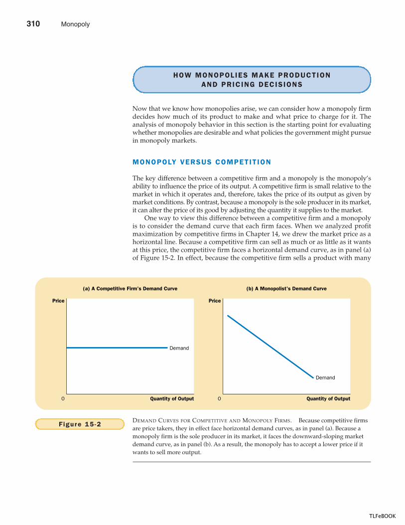
320 PART F IVE FIRM BEHAVIOR AND THE ORGANIZATION OF INDUSTRY
HOW MONOPOLIES MAKE PRODUCTIONAND PRICING DECISIONS
Now that we know how monopolies arise, we can consider how a monopoly firmdecides how much of its product to make and what price to charge for it. Theanalysis of monopoly behavior in this section is the starting point for evaluatingwhether monopolies are desirable and what policies the government might pursuein monopoly markets.
MONOPOLY VERSUS COMPETIT ION
The key difference between a competitive firm and a monopoly is the monopoly’sability to influence the price of its output. A competitive firm is small relative to themarket in which it operates and, therefore, takes the price of its output as given bymarket conditions. By contrast, because a monopoly is the sole producer in its market,it can alter the price of its good by adjusting the quantity it supplies to the market.
One way to view this difference between a competitive firm and a monopolyis to consider the demand curve that each firm faces. When we analyzed profitmaximization by competitive firms in Chapter 14, we drew the market price as ahorizontal line. Because a competitive firm can sell as much or as little as it wantsat this price, the competitive firm faces a horizontal demand curve, as in panel (a)of Figure 15-2. In effect, because the competitive firm sells a product with many
Quantity of Output
Demand
(a) A Competitive Firm’s Demand Curve (b) A Monopolist’s Demand Curve
0
Price
Quantity of Output0
Price
Demand
Figure 15 -2DEMAND CURVES FOR COMPETITIVE AND MONOPOLY FIRMS. Because competitive firmsare price takers, they in effect face horizontal demand curves, as in panel (a). Because amonopoly firm is the sole producer in its market, it faces the downward-sloping marketdemand curve, as in panel (b). As a result, the monopoly has to accept a lower price if itwants to sell more output.
310 Monopoly
TLFeBOOK
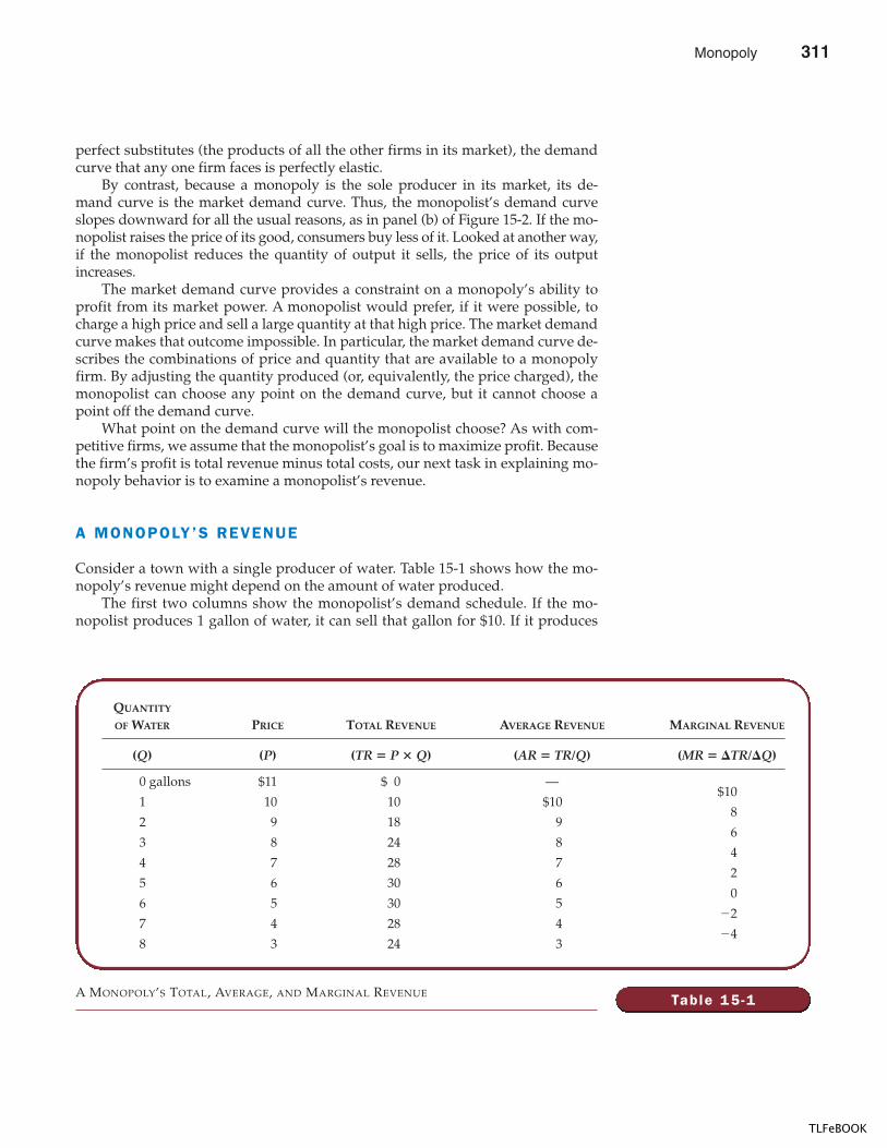
CHAPTER 15 MONOPOLY 321
perfect substitutes (the products of all the other firms in its market), the demandcurve that any one firm faces is perfectly elastic.
By contrast, because a monopoly is the sole producer in its market, its de-mand curve is the market demand curve. Thus, the monopolist’s demand curveslopes downward for all the usual reasons, as in panel (b) of Figure 15-2. If the mo-nopolist raises the price of its good, consumers buy less of it. Looked at another way,if the monopolist reduces the quantity of output it sells, the price of its outputincreases.
The market demand curve provides a constraint on a monopoly’s ability toprofit from its market power. A monopolist would prefer, if it were possible, tocharge a high price and sell a large quantity at that high price. The market demandcurve makes that outcome impossible. In particular, the market demand curve de-scribes the combinations of price and quantity that are available to a monopolyfirm. By adjusting the quantity produced (or, equivalently, the price charged), themonopolist can choose any point on the demand curve, but it cannot choose apoint off the demand curve.
What point on the demand curve will the monopolist choose? As with com-petitive firms, we assume that the monopolist’s goal is to maximize profit. Becausethe firm’s profit is total revenue minus total costs, our next task in explaining mo-nopoly behavior is to examine a monopolist’s revenue.
A MONOPOLY’S REVENUE
Consider a town with a single producer of water. Table 15-1 shows how the mo-nopoly’s revenue might depend on the amount of water produced.
The first two columns show the monopolist’s demand schedule. If the mo-nopolist produces 1 gallon of water, it can sell that gallon for $10. If it produces
Table 15 -1
QUANTITY
OF WATER PRICE TOTAL REVENUE AVERAGE REVENUE MARGINAL REVENUE
(Q) (P) (TR � P � Q) (AR � TR/Q) (MR � �TR/�Q)
0 gallons $11 $ 0 —$10
1 10 10 $108
2 9 18 96
3 8 24 84
4 7 28 72
5 6 30 60
6 5 30 5�2
7 4 28 4�4
8 3 24 3
A MONOPOLY’S TOTAL, AVERAGE, AND MARGINAL REVENUE
Monopoly 311
TLFeBOOK
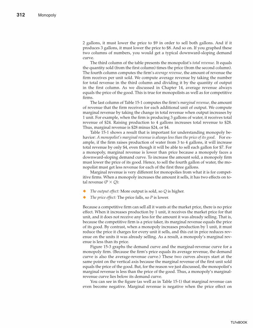
322 PART F IVE FIRM BEHAVIOR AND THE ORGANIZATION OF INDUSTRY
2 gallons, it must lower the price to $9 in order to sell both gallons. And if itproduces 3 gallons, it must lower the price to $8. And so on. If you graphed thesetwo columns of numbers, you would get a typical downward-sloping demandcurve.
The third column of the table presents the monopolist’s total revenue. It equalsthe quantity sold (from the first column) times the price (from the second column).The fourth column computes the firm’s average revenue, the amount of revenue thefirm receives per unit sold. We compute average revenue by taking the numberfor total revenue in the third column and dividing it by the quantity of outputin the first column. As we discussed in Chapter 14, average revenue alwaysequals the price of the good. This is true for monopolists as well as for competitivefirms.
The last column of Table 15-1 computes the firm’s marginal revenue, the amountof revenue that the firm receives for each additional unit of output. We computemarginal revenue by taking the change in total revenue when output increases by1 unit. For example, when the firm is producing 3 gallons of water, it receives totalrevenue of $24. Raising production to 4 gallons increases total revenue to $28.Thus, marginal revenue is $28 minus $24, or $4.
Table 15-1 shows a result that is important for understanding monopoly be-havior: A monopolist’s marginal revenue is always less than the price of its good. For ex-ample, if the firm raises production of water from 3 to 4 gallons, it will increasetotal revenue by only $4, even though it will be able to sell each gallon for $7. Fora monopoly, marginal revenue is lower than price because a monopoly faces adownward-sloping demand curve. To increase the amount sold, a monopoly firmmust lower the price of its good. Hence, to sell the fourth gallon of water, the mo-nopolist must get less revenue for each of the first three gallons.
Marginal revenue is very different for monopolies from what it is for compet-itive firms. When a monopoly increases the amount it sells, it has two effects on to-tal revenue (P � Q):
� The output effect: More output is sold, so Q is higher.� The price effect: The price falls, so P is lower.
Because a competitive firm can sell all it wants at the market price, there is no priceeffect. When it increases production by 1 unit, it receives the market price for thatunit, and it does not receive any less for the amount it was already selling. That is,because the competitive firm is a price taker, its marginal revenue equals the priceof its good. By contrast, when a monopoly increases production by 1 unit, it mustreduce the price it charges for every unit it sells, and this cut in price reduces rev-enue on the units it was already selling. As a result, a monopoly’s marginal rev-enue is less than its price.
Figure 15-3 graphs the demand curve and the marginal-revenue curve for amonopoly firm. (Because the firm’s price equals its average revenue, the demandcurve is also the average-revenue curve.) These two curves always start at thesame point on the vertical axis because the marginal revenue of the first unit soldequals the price of the good. But, for the reason we just discussed, the monopolist’smarginal revenue is less than the price of the good. Thus, a monopoly’s marginal-revenue curve lies below its demand curve.
You can see in the figure (as well as in Table 15-1) that marginal revenue caneven become negative. Marginal revenue is negative when the price effect on
312 Monopoly
TLFeBOOK
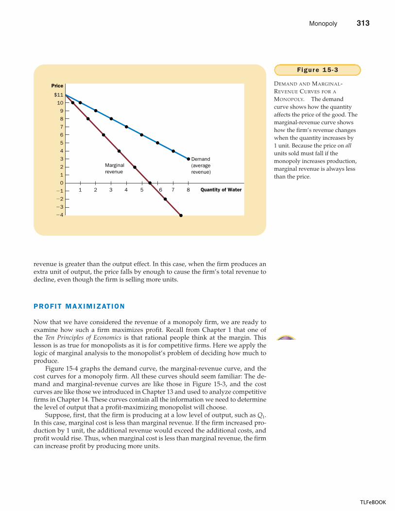
CHAPTER 15 MONOPOLY 323
revenue is greater than the output effect. In this case, when the firm produces anextra unit of output, the price falls by enough to cause the firm’s total revenue todecline, even though the firm is selling more units.
PROFIT MAXIMIZATION
Now that we have considered the revenue of a monopoly firm, we are ready toexamine how such a firm maximizes profit. Recall from Chapter 1 that one ofthe Ten Principles of Economics is that rational people think at the margin. Thislesson is as true for monopolists as it is for competitive firms. Here we apply thelogic of marginal analysis to the monopolist’s problem of deciding how much toproduce.
Figure 15-4 graphs the demand curve, the marginal-revenue curve, and thecost curves for a monopoly firm. All these curves should seem familiar: The de-mand and marginal-revenue curves are like those in Figure 15-3, and the costcurves are like those we introduced in Chapter 13 and used to analyze competitivefirms in Chapter 14. These curves contain all the information we need to determinethe level of output that a profit-maximizing monopolist will choose.
Suppose, first, that the firm is producing at a low level of output, such as Q1.In this case, marginal cost is less than marginal revenue. If the firm increased pro-duction by 1 unit, the additional revenue would exceed the additional costs, andprofit would rise. Thus, when marginal cost is less than marginal revenue, the firmcan increase profit by producing more units.
Quantity of Water
Price
$11
10
9
8
7
6
5
4
3
2
1
0
�1
�2
�3
�4
Demand(averagerevenue)
Marginalrevenue
1 2 3 4 5 6 7 8
Figure 15 -3
DEMAND AND MARGINAL-REVENUE CURVES FOR A
MONOPOLY. The demandcurve shows how the quantityaffects the price of the good. Themarginal-revenue curve showshow the firm’s revenue changeswhen the quantity increases by1 unit. Because the price on allunits sold must fall if themonopoly increases production,marginal revenue is always lessthan the price.
Monopoly 313
TLFeBOOK
324 PART F IVE FIRM BEHAVIOR AND THE ORGANIZATION OF INDUSTRY
A similar argument applies at high levels of output, such as Q2. In this case,marginal cost is greater than marginal revenue. If the firm reduced production by1 unit, the costs saved would exceed the revenue lost. Thus, if marginal cost isgreater than marginal revenue, the firm can raise profit by reducing production.
In the end, the firm adjusts its level of production until the quantity reachesQMAX, at which marginal revenue equals marginal cost. Thus, the monopolist’s profit-maximizing quantity of output is determined by the intersection of the marginal-revenuecurve and the marginal-cost curve. In Figure 15-4, this intersection occurs at point A.
You might recall from Chapter 14 that competitive firms also choose the quan-tity of output at which marginal revenue equals marginal cost. In following thisrule for profit maximization, competitive firms and monopolies are alike. But thereis also an important difference between these types of firm: The marginal revenueof a competitive firm equals its price, whereas the marginal revenue of a monop-oly is less than its price. That is,
For a competitive firm: P � MR � MC.For a monopoly firm: P > MR � MC.
The equality of marginal revenue and marginal cost at the profit-maximizingquantity is the same for both types of firm. What differs is the relationship of theprice to marginal revenue and marginal cost.
How does the monopoly find the profit-maximizing price for its product? Thedemand curve answers this question, for the demand curve relates the amountthat customers are willing to pay to the quantity sold. Thus, after the monopolyfirm chooses the quantity of output that equates marginal revenue and marginal
Monopolyprice
QuantityQ1 Q2QMAX0
Costs andRevenue
Demand
Average total cost
Marginal revenue
Marginalcost
B
1. The intersection of themarginal-revenue curveand the marginal-costcurve determines theprofit-maximizingquantity . . .
A
2. . . . and then the demandcurve shows the priceconsistent with this quantity.
Figure 15 -4
PROFIT MAXIMIZATION FOR A
MONOPOLY. A monopolymaximizes profit by choosing thequantity at which marginalrevenue equals marginal cost(point A). It then uses thedemand curve to find the pricethat will induce consumers tobuy that quantity (point B).
314 Monopoly
TLFeBOOK
CHAPTER 15 MONOPOLY 325
cost, it uses the demand curve to find the price consistent with that quantity. InFigure 15-4, the profit-maximizing price is found at point B.
We can now see a key difference between markets with competitive firms andmarkets with a monopoly firm: In competitive markets, price equals marginal cost. Inmonopolized markets, price exceeds marginal cost. As we will see in a moment, thisfinding is crucial to understanding the social cost of monopoly.
A MONOPOLY’S PROFIT
How much profit does the monopoly make? To see the monopoly’s profit, recallthat profit equals total revenue (TR) minus total costs (TC):
Profit � TR � TC.
We can rewrite this as
Profit � (TR/Q � TC/Q) � Q.
TR/Q is average revenue, which equals the price P, and TC/Q is average total costATC. Therefore,
Profit � (P � ATC) � Q.
This equation for profit (which is the same as the profit equation for competitivefirms) allows us to measure the monopolist’s profit in our graph.
Consider the shaded box in Figure 15-5. The height of the box (the segmentBC) is price minus average total cost, P – ATC, which is the profit on the typicalunit sold. The width of the box (the segment DC) is the quantity sold QMAX. There-fore, the area of this box is the monopoly firm’s total profit.
You may have noticed that wehave analyzed the price in amonopoly market using themarket demand curve and thefirm’s cost curves. We have notmade any mention of the mar-ket supply curve. By contrast,when we analyzed prices incompetitive markets beginningin Chapter 4, the two most im-portant words were always sup-ply and demand.
What happened to the sup-ply curve? Although monopoly firms make decisions aboutwhat quantity to supply (in the way described in this chapter),a monopoly does not have a supply curve. A supply curve
tells us the quantity that firms choose to supply at any givenprice. This concept makes sense when we are analyzing com-petitive firms, which are price takers. But a monopoly firm isa price maker, not a price taker. It is not meaningful to askwhat such a firm would produce at any price because thefirm sets the price at the same time it chooses the quantityto supply.
Indeed, the monopolist’s decision about how much tosupply is impossible to separate from the demand curve itfaces. The shape of the demand curve determines theshape of the marginal-revenue curve, which in turn deter-mines the monopolist’s profit-maximizing quantity. In a com-petitive market, supply decisions can be analyzed withoutknowing the demand curve, but that is not true in a monop-oly market. Therefore, we never talk about a monopoly’ssupply curve.
FYIWhy a
Monopoly DoesNot Have a
Supply Curve
Monopoly 315
TLFeBOOK
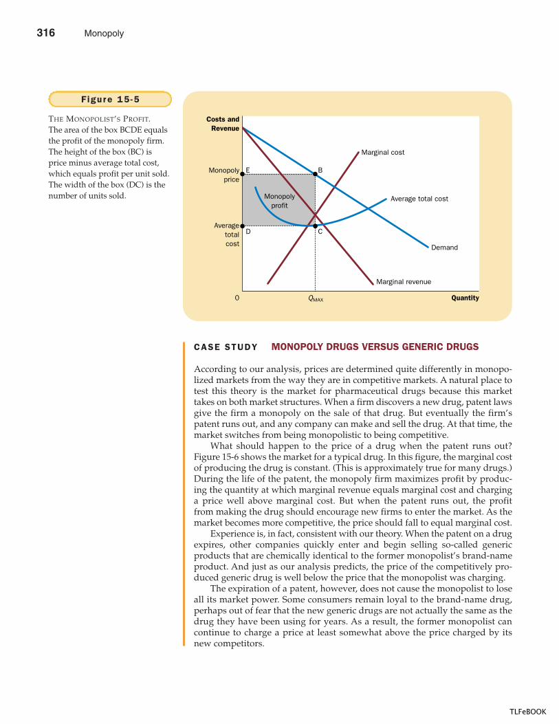
326 PART F IVE FIRM BEHAVIOR AND THE ORGANIZATION OF INDUSTRY
CASE STUDY MONOPOLY DRUGS VERSUS GENERIC DRUGS
According to our analysis, prices are determined quite differently in monopo-lized markets from the way they are in competitive markets. A natural place totest this theory is the market for pharmaceutical drugs because this markettakes on both market structures. When a firm discovers a new drug, patent lawsgive the firm a monopoly on the sale of that drug. But eventually the firm’spatent runs out, and any company can make and sell the drug. At that time, themarket switches from being monopolistic to being competitive.
What should happen to the price of a drug when the patent runs out?Figure 15-6 shows the market for a typical drug. In this figure, the marginal costof producing the drug is constant. (This is approximately true for many drugs.)During the life of the patent, the monopoly firm maximizes profit by produc-ing the quantity at which marginal revenue equals marginal cost and charginga price well above marginal cost. But when the patent runs out, the profitfrom making the drug should encourage new firms to enter the market. As themarket becomes more competitive, the price should fall to equal marginal cost.
Experience is, in fact, consistent with our theory. When the patent on a drugexpires, other companies quickly enter and begin selling so-called genericproducts that are chemically identical to the former monopolist’s brand-nameproduct. And just as our analysis predicts, the price of the competitively pro-duced generic drug is well below the price that the monopolist was charging.
The expiration of a patent, however, does not cause the monopolist to loseall its market power. Some consumers remain loyal to the brand-name drug,perhaps out of fear that the new generic drugs are not actually the same as thedrug they have been using for years. As a result, the former monopolist cancontinue to charge a price at least somewhat above the price charged by itsnew competitors.
Monopolyprice
Averagetotalcost
QuantityQMAX0
Costs andRevenue
Demand
Marginal cost
Marginal revenue
B
C
E
D
Monopolyprofit
Average total cost
Figure 15 -5
THE MONOPOLIST’S PROFIT.The area of the box BCDE equalsthe profit of the monopoly firm.The height of the box (BC) isprice minus average total cost,which equals profit per unit sold.The width of the box (DC) is thenumber of units sold.
316 Monopoly
TLFeBOOK
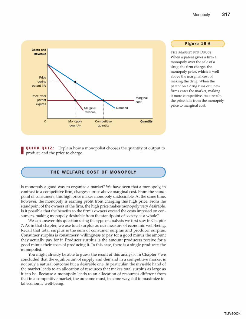
CHAPTER 15 MONOPOLY 327
QUICK QUIZ: Explain how a monopolist chooses the quantity of output to produce and the price to charge.
THE WELFARE COST OF MONOPOLY
Is monopoly a good way to organize a market? We have seen that a monopoly, incontrast to a competitive firm, charges a price above marginal cost. From the stand-point of consumers, this high price makes monopoly undesirable. At the same time,however, the monopoly is earning profit from charging this high price. From thestandpoint of the owners of the firm, the high price makes monopoly very desirable.Is it possible that the benefits to the firm’s owners exceed the costs imposed on con-sumers, making monopoly desirable from the standpoint of society as a whole?
We can answer this question using the type of analysis we first saw in Chapter7. As in that chapter, we use total surplus as our measure of economic well-being.Recall that total surplus is the sum of consumer surplus and producer surplus.Consumer surplus is consumers’ willingness to pay for a good minus the amountthey actually pay for it. Producer surplus is the amount producers receive for agood minus their costs of producing it. In this case, there is a single producer: themonopolist.
You might already be able to guess the result of this analysis. In Chapter 7 weconcluded that the equilibrium of supply and demand in a competitive market isnot only a natural outcome but a desirable one. In particular, the invisible hand ofthe market leads to an allocation of resources that makes total surplus as large asit can be. Because a monopoly leads to an allocation of resources different fromthat in a competitive market, the outcome must, in some way, fail to maximize to-tal economic well-being.
Priceduring
patent life
Price afterpatent
expires
QuantityMonopolyquantity
Competitivequantity
0
Costs andRevenue
Demand
Marginalcost
Marginalrevenue
Figure 15 -6
THE MARKET FOR DRUGS.When a patent gives a firm amonopoly over the sale of adrug, the firm charges themonopoly price, which is wellabove the marginal cost ofmaking the drug. When thepatent on a drug runs out, newfirms enter the market, makingit more competitive. As a result,the price falls from the monopolyprice to marginal cost.
Monopoly 317
TLFeBOOK
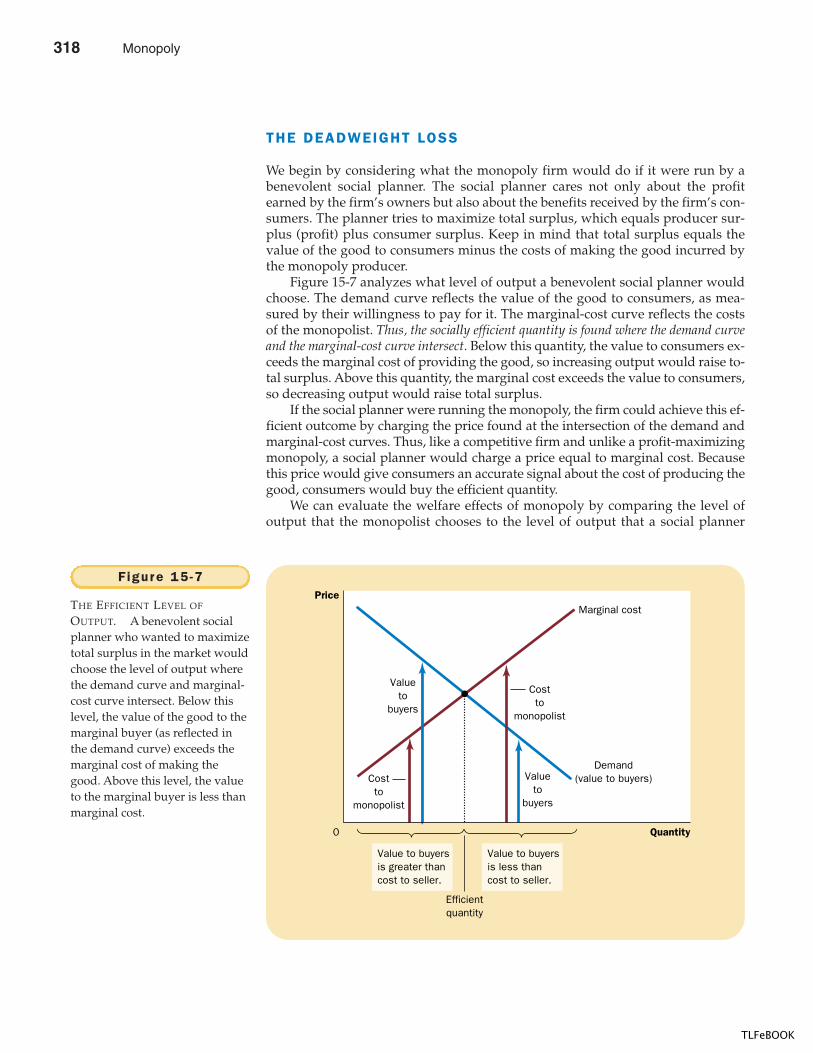
328 PART F IVE FIRM BEHAVIOR AND THE ORGANIZATION OF INDUSTRY
THE DEADWEIGHT LOSS
We begin by considering what the monopoly firm would do if it were run by abenevolent social planner. The social planner cares not only about the profitearned by the firm’s owners but also about the benefits received by the firm’s con-sumers. The planner tries to maximize total surplus, which equals producer sur-plus (profit) plus consumer surplus. Keep in mind that total surplus equals thevalue of the good to consumers minus the costs of making the good incurred bythe monopoly producer.
Figure 15-7 analyzes what level of output a benevolent social planner wouldchoose. The demand curve reflects the value of the good to consumers, as mea-sured by their willingness to pay for it. The marginal-cost curve reflects the costsof the monopolist. Thus, the socially efficient quantity is found where the demand curveand the marginal-cost curve intersect. Below this quantity, the value to consumers ex-ceeds the marginal cost of providing the good, so increasing output would raise to-tal surplus. Above this quantity, the marginal cost exceeds the value to consumers,so decreasing output would raise total surplus.
If the social planner were running the monopoly, the firm could achieve this ef-ficient outcome by charging the price found at the intersection of the demand andmarginal-cost curves. Thus, like a competitive firm and unlike a profit-maximizingmonopoly, a social planner would charge a price equal to marginal cost. Becausethis price would give consumers an accurate signal about the cost of producing thegood, consumers would buy the efficient quantity.
We can evaluate the welfare effects of monopoly by comparing the level ofoutput that the monopolist chooses to the level of output that a social planner
Quantity0
Price
Demand(value to buyers)
Efficientquantity
Marginal cost
Value to buyersis greater thancost to seller.
Value to buyersis less thancost to seller.
Costto
monopolist
Costto
monopolist
Valueto
buyers
Valueto
buyers
Figure 15 -7
THE EFFICIENT LEVEL OF
OUTPUT. A benevolent socialplanner who wanted to maximizetotal surplus in the market wouldchoose the level of output wherethe demand curve and marginal-cost curve intersect. Below thislevel, the value of the good to themarginal buyer (as reflected inthe demand curve) exceeds themarginal cost of making thegood. Above this level, the valueto the marginal buyer is less thanmarginal cost.
318 Monopoly
TLFeBOOK
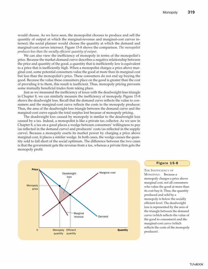
CHAPTER 15 MONOPOLY 329
would choose. As we have seen, the monopolist chooses to produce and sell thequantity of output at which the marginal-revenue and marginal-cost curves in-tersect; the social planner would choose the quantity at which the demand andmarginal-cost curves intersect. Figure 15-8 shows the comparison. The monopolistproduces less than the socially efficient quantity of output.
We can also view the inefficiency of monopoly in terms of the monopolist’sprice. Because the market demand curve describes a negative relationship betweenthe price and quantity of the good, a quantity that is inefficiently low is equivalentto a price that is inefficiently high. When a monopolist charges a price above mar-ginal cost, some potential consumers value the good at more than its marginal costbut less than the monopolist’s price. These consumers do not end up buying thegood. Because the value these consumers place on the good is greater than the costof providing it to them, this result is inefficient. Thus, monopoly pricing preventssome mutually beneficial trades from taking place.
Just as we measured the inefficiency of taxes with the deadweight-loss trianglein Chapter 8, we can similarly measure the inefficiency of monopoly. Figure 15-8shows the deadweight loss. Recall that the demand curve reflects the value to con-sumers and the marginal-cost curve reflects the costs to the monopoly producer.Thus, the area of the deadweight-loss triangle between the demand curve and themarginal-cost curve equals the total surplus lost because of monopoly pricing.
The deadweight loss caused by monopoly is similar to the deadweight losscaused by a tax. Indeed, a monopolist is like a private tax collector. As we saw inChapter 8, a tax on a good places a wedge between consumers’ willingness to pay(as reflected in the demand curve) and producers’ costs (as reflected in the supplycurve). Because a monopoly exerts its market power by charging a price abovemarginal cost, it places a similar wedge. In both cases, the wedge causes the quan-tity sold to fall short of the social optimum. The difference between the two casesis that the government gets the revenue from a tax, whereas a private firm gets themonopoly profit.
Quantity0
Price
Efficientquantity
Monopolyprice
Monopolyquantity
Deadweightloss
DemandMarginalrevenue
Marginal cost
Figure 15 -8
THE INEFFICIENCY OF
MONOPOLY. Because amonopoly charges a price abovemarginal cost, not all consumerswho value the good at more thanits cost buy it. Thus, the quantityproduced and sold by amonopoly is below the sociallyefficient level. The deadweightloss is represented by the area ofthe triangle between the demandcurve (which reflects the value ofthe good to consumers) and themarginal-cost curve (whichreflects the costs of the monopolyproducer).
Monopoly 319
TLFeBOOK
330 PART F IVE FIRM BEHAVIOR AND THE ORGANIZATION OF INDUSTRY
THE MONOPOLY’S PROFIT : A SOCIAL COST?
It is tempting to decry monopolies for “profiteering” at the expense of the public.And, indeed, a monopoly firm does earn a higher profit by virtue of its marketpower. According to the economic analysis of monopoly, however, the firm’s profitis not in itself necessarily a problem for society.
Welfare in a monopolized market, like all markets, includes the welfare of bothconsumers and producers. Whenever a consumer pays an extra dollar to a producerbecause of a monopoly price, the consumer is worse off by a dollar, and the produceris better off by the same amount. This transfer from the consumers of the good to theowners of the monopoly does not affect the market’s total surplus—the sum of con-sumer and producer surplus. In other words, the monopoly profit itself does notrepresent a shrinkage in the size of the economic pie; it merely represents a biggerslice for producers and a smaller slice for consumers. Unless consumers are for somereason more deserving than producers—a judgment that goes beyond the realm ofeconomic efficiency—the monopoly profit is not a social problem.
The problem in a monopolized market arises because the firm produces andsells a quantity of output below the level that maximizes total surplus. The dead-weight loss measures how much the economic pie shrinks as a result. This ineffi-ciency is connected to the monopoly’s high price: Consumers buy fewer unitswhen the firm raises its price above marginal cost. But keep in mind that the profitearned on the units that continue to be sold is not the problem. The problem stemsfrom the inefficiently low quantity of output. Put differently, if the high monopolyprice did not discourage some consumers from buying the good, it would raiseproducer surplus by exactly the amount it reduced consumer surplus, leaving to-tal surplus the same as could be achieved by a benevolent social planner.
There is, however, a possible exception to this conclusion. Suppose that a mo-nopoly firm has to incur additional costs to maintain its monopoly position. Forexample, a firm with a government-created monopoly might need to hire lobbyiststo convince lawmakers to continue its monopoly. In this case, the monopoly mayuse up some of its monopoly profits paying for these additional costs. If so, the so-cial loss from monopoly includes both these costs and the deadweight loss result-ing from a price above marginal cost.
QUICK QUIZ: How does a monopolist’s quantity of output compare to thequantity of output that maximizes total surplus?
PUBLIC POLICY TOWARD MONOPOLIES
We have seen that monopolies, in contrast to competitive markets, fail to allocateresources efficiently. Monopolies produce less than the socially desirable quantityof output and, as a result, charge prices above marginal cost. Policymakers in thegovernment can respond to the problem of monopoly in one of four ways:
� By trying to make monopolized industries more competitive� By regulating the behavior of the monopolies
320 Monopoly
TLFeBOOK
CHAPTER 15 MONOPOLY 331
� By turning some private monopolies into public enterprises� By doing nothing at all
INCREASING COMPETIT ION WITH ANTITRUST LAWS
If Coca-Cola and Pepsico wanted to merge, the deal would be closely examined bythe federal government before it went into effect. The lawyers and economists inthe Department of Justice might well decide that a merger between these two largesoft drink companies would make the U.S. soft drink market substantially lesscompetitive and, as a result, would reduce the economic well-being of the countryas a whole. If so, the Justice Department would challenge the merger in court, andif the judge agreed, the two companies would not be allowed to merge. It is pre-cisely this kind of challenge that prevented software giant Microsoft from buyingIntuit in 1994.
The government derives this power over private industry from the antitrustlaws, a collection of statutes aimed at curbing monopoly power. The first and mostimportant of these laws was the Sherman Antitrust Act, which Congress passed in1890 to reduce the market power of the large and powerful “trusts” that wereviewed as dominating the economy at the time. The Clayton Act, passed in 1914,strengthened the government’s powers and authorized private lawsuits. As theU.S. Supreme Court once put it, the antitrust laws are “a comprehensive charter ofeconomic liberty aimed at preserving free and unfettered competition as the ruleof trade.”
“But if we do merge with Amalgamated, we’ll have enough resources to fight theanti-trust violation caused by the merger.”
Monopoly 321
TLFeBOOK
332 PART F IVE FIRM BEHAVIOR AND THE ORGANIZATION OF INDUSTRY
The antitrust laws give the government various ways to promote competition.They allow the government to prevent mergers, such as our hypothetical mergerbetween Coca-Cola and Pepsico. They also allow the government to break up com-panies. For example, in 1984 the government split up AT&T, the large telecommu-nications company, into eight smaller companies. Finally, the antitrust laws preventcompanies from coordinating their activities in ways that make markets less com-petitive; we will discuss some of these uses of the antitrust laws in Chapter 16.
Antitrust laws have costs as well as benefits. Sometimes companies merge notto reduce competition but to lower costs through more efficient joint production.These benefits from mergers are sometimes called synergies. For example, manyU.S. banks have merged in recent years and, by combining operations, have beenable to reduce administrative staff. If antitrust laws are to raise social welfare, thegovernment must be able to determine which mergers are desirable and which arenot. That is, it must be able to measure and compare the social benefit from syner-gies to the social costs of reduced competition. Critics of the antitrust laws areskeptical that the government can perform the necessary cost-benefit analysis withsufficient accuracy.
REGULATION
Another way in which the government deals with the problem of monopoly is byregulating the behavior of monopolists. This solution is common in the case of nat-ural monopolies, such as water and electric companies. These companies are notallowed to charge any price they want. Instead, government agencies regulatetheir prices.
What price should the government set for a natural monopoly? This questionis not as easy as it might at first appear. One might conclude that the price shouldequal the monopolist’s marginal cost. If price equals marginal cost, customers willbuy the quantity of the monopolist’s output that maximizes total surplus, and theallocation of resources will be efficient.
There are, however, two practical problems with marginal-cost pricing as aregulatory system. The first is illustrated in Figure 15-9. Natural monopolies, bydefinition, have declining average total cost. As we discussed in Chapter 13, whenaverage total cost is declining, marginal cost is less than average total cost. If regu-lators are to set price equal to marginal cost, that price will be less than the firm’saverage total cost, and the firm will lose money. Instead of charging such a lowprice, the monopoly firm would just exit the industry.
Regulators can respond to this problem in various ways, none of which is per-fect. One way is to subsidize the monopolist. In essence, the government picks upthe losses inherent in marginal-cost pricing. Yet to pay for the subsidy, the govern-ment needs to raise money through taxation, which involves its own deadweightlosses. Alternatively, the regulators can allow the monopolist to charge a pricehigher than marginal cost. If the regulated price equals average total cost, the mo-nopolist earns exactly zero economic profit. Yet average-cost pricing leads to dead-weight losses, because the monopolist’s price no longer reflects the marginal costof producing the good. In essence, average-cost pricing is like a tax on the good themonopolist is selling.
The second problem with marginal-cost pricing as a regulatory system (andwith average-cost pricing as well) is that it gives the monopolist no incentive to
322 Monopoly
TLFeBOOK
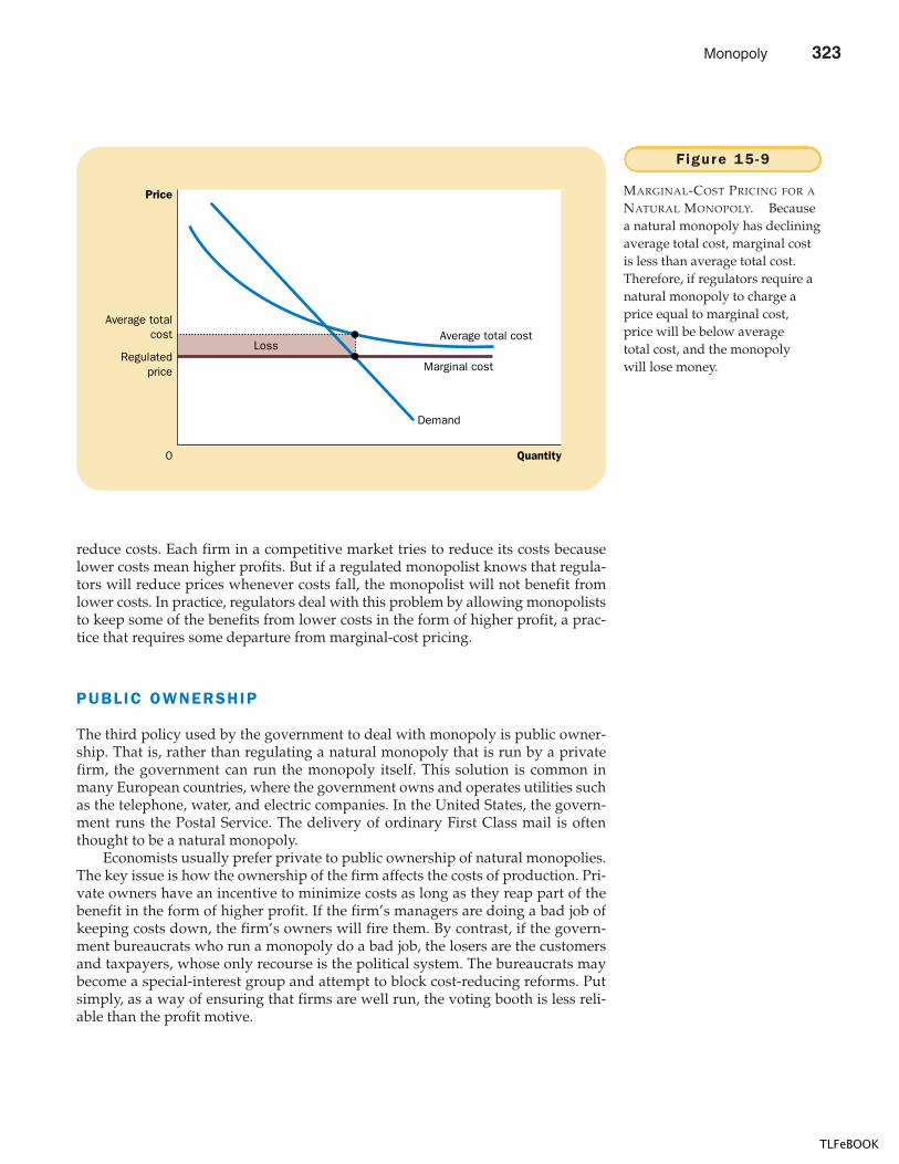
CHAPTER 15 MONOPOLY 333
reduce costs. Each firm in a competitive market tries to reduce its costs becauselower costs mean higher profits. But if a regulated monopolist knows that regula-tors will reduce prices whenever costs fall, the monopolist will not benefit fromlower costs. In practice, regulators deal with this problem by allowing monopoliststo keep some of the benefits from lower costs in the form of higher profit, a prac-tice that requires some departure from marginal-cost pricing.
PUBLIC OWNERSHIP
The third policy used by the government to deal with monopoly is public owner-ship. That is, rather than regulating a natural monopoly that is run by a privatefirm, the government can run the monopoly itself. This solution is common inmany European countries, where the government owns and operates utilities suchas the telephone, water, and electric companies. In the United States, the govern-ment runs the Postal Service. The delivery of ordinary First Class mail is oftenthought to be a natural monopoly.
Economists usually prefer private to public ownership of natural monopolies.The key issue is how the ownership of the firm affects the costs of production. Pri-vate owners have an incentive to minimize costs as long as they reap part of thebenefit in the form of higher profit. If the firm’s managers are doing a bad job ofkeeping costs down, the firm’s owners will fire them. By contrast, if the govern-ment bureaucrats who run a monopoly do a bad job, the losers are the customersand taxpayers, whose only recourse is the political system. The bureaucrats maybecome a special-interest group and attempt to block cost-reducing reforms. Putsimply, as a way of ensuring that firms are well run, the voting booth is less reli-able than the profit motive.
Average totalcost
Regulatedprice
Quantity0
Loss
Price
Demand
Marginal cost
Average total cost
Figure 15 -9
MARGINAL-COST PRICING FOR A
NATURAL MONOPOLY. Becausea natural monopoly has decliningaverage total cost, marginal costis less than average total cost.Therefore, if regulators require anatural monopoly to charge aprice equal to marginal cost,price will be below averagetotal cost, and the monopolywill lose money.
Monopoly 323
TLFeBOOK
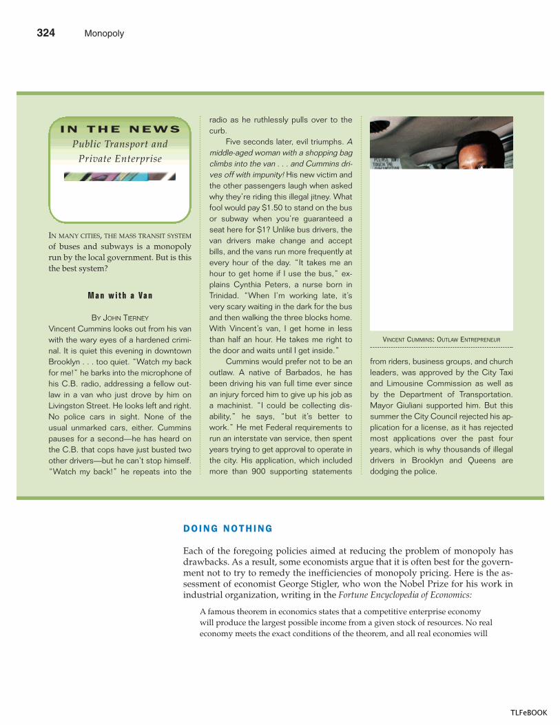
334 PART F IVE FIRM BEHAVIOR AND THE ORGANIZATION OF INDUSTRY
DOING NOTHING
Each of the foregoing policies aimed at reducing the problem of monopoly hasdrawbacks. As a result, some economists argue that it is often best for the govern-ment not to try to remedy the inefficiencies of monopoly pricing. Here is the as-sessment of economist George Stigler, who won the Nobel Prize for his work inindustrial organization, writing in the Fortune Encyclopedia of Economics:
A famous theorem in economics states that a competitive enterprise economywill produce the largest possible income from a given stock of resources. No realeconomy meets the exact conditions of the theorem, and all real economies will
IN MANY CITIES, THE MASS TRANSIT SYSTEM
of buses and subways is a monopolyrun by the local government. But is thisthe best system?
M a n w i t h a Va n
BY JOHN TIERNEY
Vincent Cummins looks out from his vanwith the wary eyes of a hardened crimi-nal. It is quiet this evening in downtownBrooklyn . . . too quiet. “Watch my backfor me!” he barks into the microphone ofhis C.B. radio, addressing a fellow out-law in a van who just drove by him onLivingston Street. He looks left and right.No police cars in sight. None of theusual unmarked cars, either. Cumminspauses for a second—he has heard onthe C.B. that cops have just busted twoother drivers—but he can’t stop himself.“Watch my back!” he repeats into the
radio as he ruthlessly pulls over to thecurb.
Five seconds later, evil triumphs. Amiddle-aged woman with a shopping bagclimbs into the van . . . and Cummins dri-ves off with impunity! His new victim andthe other passengers laugh when askedwhy they’re riding this illegal jitney. Whatfool would pay $1.50 to stand on the busor subway when you’re guaranteed aseat here for $1? Unlike bus drivers, thevan drivers make change and acceptbills, and the vans run more frequently atevery hour of the day. “It takes me anhour to get home if I use the bus,” ex-plains Cynthia Peters, a nurse born inTrinidad. “When I’m working late, it’svery scary waiting in the dark for the busand then walking the three blocks home.With Vincent’s van, I get home in lessthan half an hour. He takes me right tothe door and waits until I get inside.”
Cummins would prefer not to be anoutlaw. A native of Barbados, he hasbeen driving his van full time ever sincean injury forced him to give up his job asa machinist. “I could be collecting dis-ability,” he says, “but it’s better towork.” He met Federal requirements torun an interstate van service, then spentyears trying to get approval to operate inthe city. His application, which includedmore than 900 supporting statements
from riders, business groups, and churchleaders, was approved by the City Taxiand Limousine Commission as well asby the Department of Transportation.Mayor Giuliani supported him. But thissummer the City Council rejected his ap-plication for a license, as it has rejectedmost applications over the past fouryears, which is why thousands of illegaldrivers in Brooklyn and Queens aredodging the police.
IN THE NEWS
Public Transport andPrivate Enterprise
VINCENT CUMMINS: OUTLAW ENTREPRENEUR
324 Monopoly
TLFeBOOK
CHAPTER 15 MONOPOLY 335
fall short of the ideal economy—a difference called “market failure.” In my view,however, the degree of “market failure” for the American economy is muchsmaller than the “political failure” arising from the imperfections of economicpolicies found in real political systems.
As this quotation makes clear, determining the proper role of the government inthe economy requires judgments about politics as well as economics.
QUICK QUIZ: Describe the ways policymakers can respond to the inefficiencies caused by monopolies. List a potential problem with each of these policy responses.
Council members claim they’re try-ing to prevent vans from causing acci-dents and traffic problems, although noone who rides the vans takes theseprotestations seriously. Vans with accred-ited and insured drivers like Cummins areno more dangerous or disruptive thantaxis. The only danger they pose is to thepublic transit monopoly, whose unionleaders have successfully led the cam-paign against them.
The van drivers have refuted twomodern urban myths: that mass transitmust lose money and that it must be apublic enterprise. Entrepreneurs likeCummins are thriving today in othercities—Seoul and Buenos Aires rely en-tirely on private, profitable bus compa-nies—and they once made New York theworld leader in mass transit. The firsthorsecars and elevated trains were de-veloped here by private companies. Thefirst subway was partly financed with aloan from the city, but it was otherwise aprivate operation, built and run quiteprofitably with the fare set at a nickel—the equivalent of less than a dollar today.
Eventually though, New York’s politi-cians drove most private transit compa-nies out of business by refusing to adjustthe fare for inflation. When the enter-prises lost money in the 1920’s, MayorJohn Hylan offered to teach them efficient
management. If the city ran the subway,he promised, it would make money whilepreserving the nickel fare and freeingNew Yorkers from “serfdom” and “dicta-torship” of the “grasping transportationmonopolies.” But expenses soared assoon as government merged the privatesystems into a true monopoly. The fare,which remained a nickel through sevendecades of private transit, has risen 2,900percent under public management—andtoday the Metropolitan Transportation Au-thority still manages to lose about $2 perride. Meanwhile, a jitney driver can pro-vide better service at lower prices and stillmake a profit.
“Transit could be profitable again ifentrepreneurs are given a chance,” saysDaniel B. Klein, an economist at SantaClara University in California and the co-author of Curb Rights, a new book fromthe Brookings Institution on mass transit.“Government has demonstrated that ithas no more business producing transitthan producing cornflakes. It should con-centrate instead on establishing newrules to foster competition.” To encour-age private operators to make a long-term investment in regular service alonga route, the Brookings researchers rec-ommend selling them exclusive “curbrights” to pick up passengers waiting atcertain stops along the route. That way
part-time opportunists couldn’t swoop into steal regular customers from a long-term operator. But to encourage compe-tition, at other corners along the routethere should also be common stopswhere passengers could be picked up byany licensed jitney or bus.
Elements of this system already ex-ist where jitneys have informally estab-lished their own stops separate from theregular buses, but the City Council is try-ing to eliminate these competitors. Be-sides denying licenses to new driverslike Cummins, the Council has forbiddenveteran drivers with licenses to operateon bus routes. Unless these restrictionsare overturned in court—a suit on thedrivers’ behalf has been filed by the Insti-tute for Justice, a public-interest law firmin Washington—the vans can competeonly by breaking the law. At this very mo-ment, despite the best efforts of the po-lice and the Transport Workers Union,somewhere in New York a serial preda-tor like Cummins is luring another unsus-pecting victim. He may even be makingchange for a $5 bill.
SOURCE: The New York Times Magazine, August 10,1997, p. 22.
Monopoly 325
TLFeBOOK
336 PART F IVE FIRM BEHAVIOR AND THE ORGANIZATION OF INDUSTRY
PRICE DISCRIMINATION
So far we have been assuming that the monopoly firm charges the same price to allcustomers. Yet in many cases firms try to sell the same good to different customersfor different prices, even though the costs of producing for the two customers arethe same. This practice is called price discrimination.
Before discussing the behavior of a price-discriminating monopolist, weshould note that price discrimination is not possible when a good is sold in a com-petitive market. In a competitive market, there are many firms selling the samegood at the market price. No firm is willing to charge a lower price to any cus-tomer because the firm can sell all it wants at the market price. And if any firmtried to charge a higher price to a customer, that customer would buy from anotherfirm. For a firm to price discriminate, it must have some market power.
A PARABLE ABOUT PRICING
To understand why a monopolist would want to price discriminate, let’s considera simple example. Imagine that you are the president of Readalot Publishing Com-pany. Readalot’s best-selling author has just written her latest novel. To keepthings simple, let’s imagine that you pay the author a flat $2 million for the exclu-sive rights to publish the book. Let’s also assume that the cost of printing the bookis zero. Readalot’s profit, therefore, is the revenue it gets from selling the book mi-nus the $2 million it has paid to the author. Given these assumptions, how wouldyou, as Readalot’s president, decide what price to charge for the book?
Your first step in setting the price is to estimate what the demand for the bookis likely to be. Readalot’s marketing department tells you that the book will attracttwo types of readers. The book will appeal to the author’s 100,000 die-hard fans.These fans will be willing to pay as much as $30 for the book. In addition, the bookwill appeal to about 400,000 less enthusiastic readers who will be willing to pay upto $5 for the book.
What price maximizes Readalot’s profit? There are two natural prices to con-sider: $30 is the highest price Readalot can charge and still get the 100,000 die-hardfans, and $5 is the highest price it can charge and still get the entire market of500,000 potential readers. It is a matter of simple arithmetic to solve Readalot’sproblem. At a price of $30, Readalot sells 100,000 copies, has revenue of $3 million,and makes profit of $1 million. At a price of $5, it sells 500,000 copies, has revenueof $2.5 million, and makes profit of $500,000. Thus, Readalot maximizes profit bycharging $30 and forgoing the opportunity to sell to the 400,000 less enthusiasticreaders.
Notice that Readalot’s decision causes a deadweight loss. There are 400,000readers willing to pay $5 for the book, and the marginal cost of providing it tothem is zero. Thus, $2 million of total surplus is lost when Readalot charges thehigher price. This deadweight loss is the usual inefficiency that arises whenever amonopolist charges a price above marginal cost.
Now suppose that Readalot’s marketing department makes an important dis-covery: These two groups of readers are in separate markets. All the die-hard fanslive in Australia, and all the other readers live in the United States. Moreover, it is
pr ice d iscr iminat ionthe business practice of selling thesame good at different prices todifferent customers
326 Monopoly
TLFeBOOK
CHAPTER 15 MONOPOLY 337
difficult for readers in one country to buy books in the other. How does this dis-covery affect Readalot’s marketing strategy?
In this case, the company can make even more profit. To the 100,000 Australianreaders, it can charge $30 for the book. To the 400,000 American readers, it cancharge $5 for the book. In this case, revenue is $3 million in Australia and $2 mil-lion in the United States, for a total of $5 million. Profit is then $3 million, which issubstantially greater than the $1 million the company could earn charging thesame $30 price to all customers. Not surprisingly, Readalot chooses to follow thisstrategy of price discrimination.
Although the story of Readalot Publishing is hypothetical, it describes accu-rately the business practice of many publishing companies. Textbooks, for example,are often sold at a lower price in Europe than in the United States. Even more im-portant is the price differential between hardcover books and paperbacks. When apublisher has a new novel, it initially releases an expensive hardcover edition andlater releases a cheaper paperback edition. The difference in price between these twoeditions far exceeds the difference in printing costs. The publisher’s goal is just as inour example. By selling the hardcover to die-hard fans and the paperback to less en-thusiastic readers, the publisher price discriminates and raises its profit.
THE MORAL OF THE STORY
Like any parable, the story of Readalot Publishing is stylized. Yet, also like anyparable, it teaches some important and general lessons. In this case, there are threelessons to be learned about price discrimination.
The first and most obvious lesson is that price discrimination is a rationalstrategy for a profit-maximizing monopolist. In other words, by charging differentprices to different customers, a monopolist can increase its profit. In essence, aprice-discriminating monopolist charges each customer a price closer to his or herwillingness to pay than is possible with a single price.
The second lesson is that price discrimination requires the ability to separatecustomers according to their willingness to pay. In our example, customers wereseparated geographically. But sometimes monopolists choose other differences,such as age or income, to distinguish among customers.
A corollary to this second lesson is that certain market forces can prevent firmsfrom price discriminating. In particular, one such force is arbitrage, the process ofbuying a good in one market at a low price and selling it in another market at ahigher price in order to profit from the price difference. In our example, supposethat Australian bookstores could buy the book in the United States and resell it toAustralian readers. This arbitrage would prevent Readalot from price discriminat-ing because no Australian would buy the book at the higher price.
The third lesson from our parable is perhaps the most surprising: Price dis-crimination can raise economic welfare. Recall that a deadweight loss arises whenReadalot charges a single $30 price, because the 400,000 less enthusiastic readersdo not end up with the book, even though they value it at more than its marginalcost of production. By contrast, when Readalot price discriminates, all readers endup with the book, and the outcome is efficient. Thus, price discrimination can elim-inate the inefficiency inherent in monopoly pricing.
Note that the increase in welfare from price discrimination shows up as higherproducer surplus rather than higher consumer surplus. In our example, consumers
Monopoly 327
TLFeBOOK
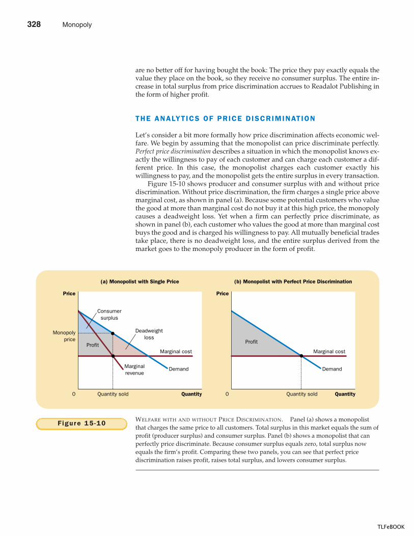
338 PART F IVE FIRM BEHAVIOR AND THE ORGANIZATION OF INDUSTRY
are no better off for having bought the book: The price they pay exactly equals thevalue they place on the book, so they receive no consumer surplus. The entire in-crease in total surplus from price discrimination accrues to Readalot Publishing inthe form of higher profit.
THE ANALYTICS OF PRICE DISCRIMINATION
Let’s consider a bit more formally how price discrimination affects economic wel-fare. We begin by assuming that the monopolist can price discriminate perfectly.Perfect price discrimination describes a situation in which the monopolist knows ex-actly the willingness to pay of each customer and can charge each customer a dif-ferent price. In this case, the monopolist charges each customer exactly hiswillingness to pay, and the monopolist gets the entire surplus in every transaction.
Figure 15-10 shows producer and consumer surplus with and without pricediscrimination. Without price discrimination, the firm charges a single price abovemarginal cost, as shown in panel (a). Because some potential customers who valuethe good at more than marginal cost do not buy it at this high price, the monopolycauses a deadweight loss. Yet when a firm can perfectly price discriminate, asshown in panel (b), each customer who values the good at more than marginal costbuys the good and is charged his willingness to pay. All mutually beneficial tradestake place, there is no deadweight loss, and the entire surplus derived from themarket goes to the monopoly producer in the form of profit.
(a) Monopolist with Single Price
Price
0 QuantityQuantity sold Quantity sold
(b) Monopolist with Perfect Price Discrimination
Price
0 Quantity
Monopolyprice
ProfitProfit
Deadweightloss
Demand Demand
Marginal cost
Marginalrevenue
Consumersurplus
Marginal cost
Figure 15 -10 WELFARE WITH AND WITHOUT PRICE DISCRIMINATION. Panel (a) shows a monopolistthat charges the same price to all customers. Total surplus in this market equals the sum ofprofit (producer surplus) and consumer surplus. Panel (b) shows a monopolist that canperfectly price discriminate. Because consumer surplus equals zero, total surplus nowequals the firm’s profit. Comparing these two panels, you can see that perfect pricediscrimination raises profit, raises total surplus, and lowers consumer surplus.
328 Monopoly
TLFeBOOK
CHAPTER 15 MONOPOLY 339
In reality, of course, price discrimination is not perfect. Customers do not walkinto stores with signs displaying their willingness to pay. Instead, firms price dis-criminate by dividing customers into groups: young versus old, weekday versusweekend shoppers, Americans versus Australians, and so on. Unlike those in ourparable of Readalot Publishing, customers within each group differ in their will-ingness to pay for the product, making perfect price discrimination impossible.
How does this imperfect price discrimination affect welfare? The analysis ofthese pricing schemes is quite complicated, and it turns out that there is no generalanswer to this question. Compared to the monopoly outcome with a single price,imperfect price discrimination can raise, lower, or leave unchanged total surplusin a market. The only certain conclusion is that price discrimination raises the mo-nopoly’s profit—otherwise the firm would choose to charge all customers thesame price.
EXAMPLES OF PRICE DISCRIMINATION
Firms in our economy use various business strategies aimed at charging differentprices to different customers. Now that we understand the economics of price dis-crimination, let’s consider some examples.
Movie T ickets Many movie theaters charge a lower price for children andsenior citizens than for other patrons. This fact is hard to explain in a competitivemarket. In a competitive market, price equals marginal cost, and the marginal costof providing a seat for a child or senior citizen is the same as the marginal cost ofproviding a seat for anyone else. Yet this fact is easily explained if movie theatershave some local monopoly power and if children and senior citizens have a lower
“Would it bother you to hear how little I paid for this flight?”
Monopoly 329
TLFeBOOK
340 PART F IVE FIRM BEHAVIOR AND THE ORGANIZATION OF INDUSTRY
WHAT ORGANIZATION IN OUR ECONOMY IS
most successful at exerting marketpower and keeping prices away fromtheir competitive levels? EconomistRobert Barro reports on the first (andonly) annual competition to find themost successful monopoly.
L e t ’s P l a y M o n o p o l y
BY ROBERT J. BARRO
It’s almost the end of summer and timefor the first annual contest to choose thebest operating monopoly in America. Thecontestants, selected by a panel of Har-vard economists, are as follows:
1. The U.S. Postal Service
2. OPEC [Organization of PetroleumExporting Countries]
3. Almost any cable TV company
4. The Ivy League universities (foradministering financial aid tostudents)
5. The NCAA [National CollegiateAthletic Association] (foradministering payments to student-athletes) . . .
Each contestant exhibits fine monopolis-tic characteristics and is worthy of seri-ous consideration for the award. TheU.S. Postal Service claims to be thelongest-running monopoly in Americaand has the distinction of having its con-trol over First Class mail prescribed (per-haps) by the Constitution. The monopolyhas preserved large flows of revenuesand high wage rates despite studiesshowing that private companies couldcarry the mail more efficiently at muchlower cost.
On the other hand, the position ofthe Postal Service has been eroded:first, by successful competition on pack-age delivery; second, by the recent entryof express delivery services; and third,and potentially most damaging, by the in-troduction of the fax machine. Sincefaxes are bound to supplant a substantialfraction of First Class letters, the failureto get Congress to classify a fax as FirstClass mail and, hence, the exclusive do-main of the post office shows a remark-able loss of political muscle. Thus,despite past glories, it is hard to be san-guine about the long-term prospects ofthe post office as a flourishing monopoly.
OPEC was impressive in generatingbillions of dollars for its members from1973 to the early 1980s. To understandthe functioning of this cartel it is impor-tant to sort out the good guys from thebad guys.
The good guys, like Saudi Arabia andKuwait, are the ones who have typicallyheld oil production below capacity andthereby kept prices above the competitivelevel. The bad guys, like Libya and Iraq(when Iraq was allowed to produce oil),
are the ones who have produced as muchas they could and thereby kept prices low.
The good guys were responsible forthe vast expansion of oil revenues duringthe blissful period after 1973. (Hence,they were responsible for the consider-able difficulties endured by oil con-sumers.) But, unfortunately, thesecountries could not keep the otherOPEC members in line and were also un-able to exclude new producers or pre-vent conservation by consumers. Thus,oil prices plummeted in 1986. . . .
In any event, it is unclear thatOPEC qualifies for the contest: It is notreally American, and its members would
IN THE NEWS
The Best Monopolist
IS THE NCAA THE BEST MONOPOLIST?
330 Monopoly
TLFeBOOK
CHAPTER 15 MONOPOLY 341
probably be arrested for price-fixing ifthey ever held an official meeting inAmerica.
Most cable TV companies havegovernment-issued licenses that keepcompetitors out. Thus, this businesssupports the hypothesis (offered, I think,by George Stigler) that private monopo-lies are not sustainable for long unlessthey have the weight of government be-hind them.
The rapid escalation of prices andthe limitations on services seem, how-ever, to be getting customers and theircongressional representatives progres-sively more annoyed. Thus, it would notbe surprising if legislative action leadssoon to a deterioration of the cable com-panies’ monopoly power. . . . This fearabout the future diminishes the claim ofthis otherwise worthy contestant for thefirst annual prize.
Officials of Ivy League universitieshave been able to meet in semi-public fo-rums to set rules that determine pricesof admission (tuition less financial aid) asa function of applicant characteristics,especially financial resources. In somecases, the schools pooled information toagree in advance on the right price tocharge a specific customer. Airlines andother industries that wish to price dis-criminate can only dream about this kindof setup.
Moreover, the universities havemore or less successfully applied a highmoral tone to the process: Rich appli-cants—especially smart rich applicants—are charged more than the competitiveprice for schooling in order to subsidizethe smart poor, but it is unclear why this
subsidy should come from the smart richrather than from taxpayers in general.
In any event, the universities’ envi-able cartel position has been damagedby the unenlightened Justice Depart-ment, which argued that the price-settingmeetings were a violation of antitrustlaws. Since most of the universities in-volved have agreed to stop these prac-tices, it may be that future prices forprivate higher education will come closerto being competitively determined. . . .
The final contestant, the NCAA, hasbeen remarkably successful in holdingdown “salaries” paid to college athletes.It would be one thing merely to colludeto determine price ceilings (for example,to restrict payments so that they not ex-ceed tuition plus room and board andsome minor additional amount), but theNCAA has also managed to monopolizeall the moral arguments.
Consider a poor ghetto residentwho can play basketball well, but not wellenough to make it to the NBA. If therewere no NCAA, this player might be ablelegitimately to accumulate a significantamount of cash during a four-year career.But the NCAA ensures that the playerwill remain poor after four years and,moreover, has convinced most ob-servers that it would be morally wrongfor the college to pay the player a com-petitively determined wage for his or herservices.
For many economists, this interfer-ence with competition—in a setting thathas no obvious reasons for market fail-ure—is itself morally repugnant. But theoutrage is compounded here becausethe transfer is clearly from poor ghetto
residents to rich colleges. Compare thesituation of contestant number 4, the IvyLeague universities, in which the transferfrom rich to poor students can readily besupported on Robin Hood grounds.
The NCAA has the much more diffi-cult task of defending a policy that pre-vents many poor individuals from earningmoney. Incredibly, this defense has beenso successful that it has even allowedthe organization to maintain the moralhigh ground. When the NCAA maintainsits cartel by punishing schools that violatethe rules (by paying too much), almost noone doubts that the evil entities are theschools or people who paid the athletes,rather than the cartel enforcers who pre-vented the athletes from getting paid.Given this extraordinary balancing act,the decision of the panelists was straight-forward and the NCAA is the clear anddeserving winner of the first annual prizefor best monopoly in America.
The panel of economists also con-sidered briefly an award for the least effi-cient monopoly in America. This choicewas, however, too easy. It goes to theAmerican Economic Association, whichhas been a dismal failure at establishinglicensing requirements or other restric-tions on entry into the economics pro-fession. It is a sad state of affairs whenalmost anyone can assume the title ofeconomist.
SOURCE: The Wall Street Journal, August 27, 1991,p. A12.
Monopoly 331
TLFeBOOK
342 PART F IVE FIRM BEHAVIOR AND THE ORGANIZATION OF INDUSTRY
willingness to pay for a ticket. In this case, movie theaters raise their profit by pricediscriminating.
Ai r l ine Pr ices Seats on airplanes are sold at many different prices. Most air-lines charge a lower price for a round-trip ticket between two cities if the travelerstays over a Saturday night. At first this seems odd. Why should it matter to theairline whether a passenger stays over a Saturday night? The reason is that thisrule provides a way to separate business travelers and personal travelers. A pas-senger on a business trip has a high willingness to pay and, most likely, does notwant to stay over a Saturday night. By contrast, a passenger traveling for personalreasons has a lower willingness to pay and is more likely to be willing to stay overa Saturday night. Thus, the airlines can successfully price discriminate by charginga lower price for passengers who stay over a Saturday night.
Discount Coupons Many companies offer discount coupons to the publicin newspapers and magazines. A buyer simply has to clip out the coupon in orderto get $0.50 off his next purchase. Why do companies offer these coupons? Whydon’t they just cut the price of the product by $0.50?
The answer is that coupons allow companies to price discriminate. Companiesknow that not all customers are willing to spend the time to clip out coupons.Moreover, the willingness to clip coupons is related to the customer’s willingnessto pay for the good. A rich and busy executive is unlikely to spend her time clip-ping discount coupons out of the newspaper, and she is probably willing to pay ahigher price for many goods. A person who is unemployed is more likely to clipcoupons and has a lower willingness to pay. Thus, by charging a lower price onlyto those customers who clip coupons, firms can successfully price discriminate.
F inanc ia l A id Many colleges and universities give financial aid to needystudents. One can view this policy as a type of price discrimination. Wealthy stu-dents have greater financial resources and, therefore, a higher willingness to paythan needy students. By charging high tuition and selectively offering financialaid, schools in effect charge prices to customers based on the value they place ongoing to that school. This behavior is similar to that of any price-discriminatingmonopolist.
Quant i ty D iscounts So far in our examples of price discrimination, themonopolist charges different prices to different customers. Sometimes, however,monopolists price discriminate by charging different prices to the same customerfor different units that the customer buys. For example, many firms offer lowerprices to customers who buy large quantities. A bakery might charge $0.50 for eachdonut, but $5 for a dozen. This is a form of price discrimination because thecustomer pays a higher price for the first unit bought than for the twelfth. Quan-tity discounts are often a successful way of price discriminating because a cus-tomer’s willingness to pay for an additional unit declines as the customer buysmore units.
QUICK QUIZ: Give two examples of price discrimination. � How does perfect price discrimination affect consumer surplus, producer surplus, and total surplus?
332 Monopoly
TLFeBOOK
CHAPTER 15 MONOPOLY 343
CONCLUSION: THE PREVALENCE OF MONOPOLY
This chapter has discussed the behavior of firms that have control over the pricesthey charge. We have seen that because monopolists produce less than the sociallyefficient quantity and charge prices above marginal cost, they cause deadweightlosses. These inefficiencies can be mitigated through prudent public policies or, insome cases, through price discrimination by the monopolist.
How prevalent are the problems of monopoly? There are two answers to thisquestion.
In one sense, monopolies are common. Most firms have some control over theprices they charge. They are not forced to charge the market price for their goods,because their goods are not exactly the same as those offered by other firms. AFord Taurus is not the same as a Toyota Camry. Ben and Jerry’s ice cream is not thesame as Breyer’s. Each of these goods has a downward-sloping demand curve,which gives each producer some degree of monopoly power.
Yet firms with substantial monopoly power are quite rare. Few goods are trulyunique. Most have substitutes that, even if not exactly the same, are very similar.Ben and Jerry can raise the price of their ice cream a little without losing all theirsales; but if they raise it very much, sales will fall substantially.
In the end, monopoly power is a matter of degree. It is true that many firmshave some monopoly power. It is also true that their monopoly power is usuallyquite limited. In these cases, we will not go far wrong assuming that firms operatein competitive markets, even if that is not precisely the case.
� A monopoly is a firm that is the sole seller in its market.A monopoly arises when a single firm owns a keyresource, when the government gives a firm the exclusiveright to produce a good, or when a single firm can supplythe entire market at a smaller cost than many firms could.
� Because a monopoly is the sole producer in its market, itfaces a downward-sloping demand curve for itsproduct. When a monopoly increases production by 1unit, it causes the price of its good to fall, which reducesthe amount of revenue earned on all units produced. Asa result, a monopoly’s marginal revenue is alwaysbelow the price of its good.
� Like a competitive firm, a monopoly firm maximizesprofit by producing the quantity at which marginalrevenue equals marginal cost. The monopoly thenchooses the price at which that quantity is demanded.Unlike a competitive firm, a monopoly firm’s priceexceeds its marginal revenue, so its price exceedsmarginal cost.
� A monopolist’s profit-maximizing level of output isbelow the level that maximizes the sum of consumerand producer surplus. That is, when the monopolycharges a price above marginal cost, some consumerswho value the good more than its cost of production donot buy it. As a result, monopoly causes deadweightlosses similar to the deadweight losses caused by taxes.
� Policymakers can respond to the inefficiency ofmonopoly behavior in four ways. They can use theantitrust laws to try to make the industry morecompetitive. They can regulate the prices that themonopoly charges. They can turn the monopolist into agovernment-run enterprise. Or, if the market failure isdeemed small compared to the inevitable imperfectionsof policies, they can do nothing at all.
� Monopolists often can raise their profits by chargingdifferent prices for the same good based on a buyer’swillingness to pay. This practice of price discriminationcan raise economic welfare by getting the good to some
Summar y
Monopoly 333
TLFeBOOK
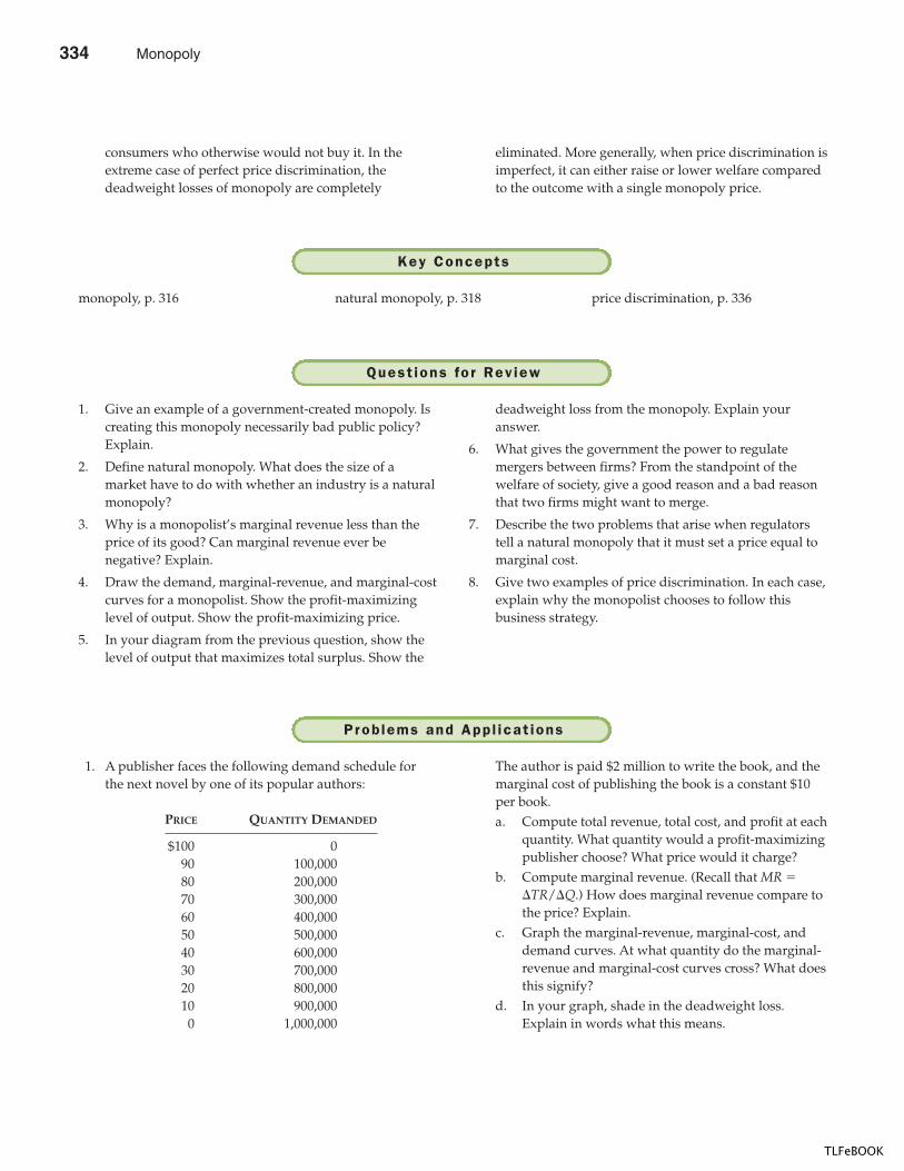
344 PART F IVE FIRM BEHAVIOR AND THE ORGANIZATION OF INDUSTRY
consumers who otherwise would not buy it. In theextreme case of perfect price discrimination, thedeadweight losses of monopoly are completely
eliminated. More generally, when price discrimination isimperfect, it can either raise or lower welfare comparedto the outcome with a single monopoly price.
monopoly, p. 316 natural monopoly, p. 318 price discrimination, p. 336
Key Concepts
1. Give an example of a government-created monopoly. Iscreating this monopoly necessarily bad public policy?Explain.
2. Define natural monopoly. What does the size of amarket have to do with whether an industry is a naturalmonopoly?
3. Why is a monopolist’s marginal revenue less than theprice of its good? Can marginal revenue ever benegative? Explain.
4. Draw the demand, marginal-revenue, and marginal-costcurves for a monopolist. Show the profit-maximizinglevel of output. Show the profit-maximizing price.
5. In your diagram from the previous question, show thelevel of output that maximizes total surplus. Show the
deadweight loss from the monopoly. Explain youranswer.
6. What gives the government the power to regulatemergers between firms? From the standpoint of thewelfare of society, give a good reason and a bad reasonthat two firms might want to merge.
7. Describe the two problems that arise when regulatorstell a natural monopoly that it must set a price equal tomarginal cost.
8. Give two examples of price discrimination. In each case,explain why the monopolist chooses to follow thisbusiness strategy.
Quest ions fo r Rev iew
1. A publisher faces the following demand schedule forthe next novel by one of its popular authors:
PRICE QUANTITY DEMANDED
$100 090 100,00080 200,00070 300,00060 400,00050 500,00040 600,00030 700,00020 800,00010 900,0000 1,000,000
The author is paid $2 million to write the book, and themarginal cost of publishing the book is a constant $10per book.a. Compute total revenue, total cost, and profit at each
quantity. What quantity would a profit-maximizingpublisher choose? What price would it charge?
b. Compute marginal revenue. (Recall that MR �
�TR/�Q.) How does marginal revenue compare tothe price? Explain.
c. Graph the marginal-revenue, marginal-cost, anddemand curves. At what quantity do the marginal-revenue and marginal-cost curves cross? What doesthis signify?
d. In your graph, shade in the deadweight loss.Explain in words what this means.
Prob lems and App l icat ions
334 Monopoly
TLFeBOOK
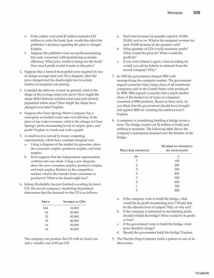
CHAPTER 15 MONOPOLY 345
e. If the author were paid $3 million instead of $2million to write the book, how would this affect thepublisher’s decision regarding the price to charge?Explain.
f. Suppose the publisher were not profit-maximizingbut were concerned with maximizing economicefficiency. What price would it charge for the book?How much profit would it make at this price?
2. Suppose that a natural monopolist were required by lawto charge average total cost. On a diagram, label theprice charged and the deadweight loss to societyrelative to marginal-cost pricing.
3. Consider the delivery of mail. In general, what is theshape of the average-total-cost curve? How might theshape differ between isolated rural areas and denselypopulated urban areas? How might the shape havechanged over time? Explain.
4. Suppose the Clean Springs Water Company has amonopoly on bottled water sales in California. If theprice of tap water increases, what is the change in CleanSprings’ profit-maximizing levels of output, price, andprofit? Explain in words and with a graph.
5. A small town is served by many competingsupermarkets, which have constant marginal cost.a. Using a diagram of the market for groceries, show
the consumer surplus, producer surplus, and totalsurplus.
b. Now suppose that the independent supermarketscombine into one chain. Using a new diagram,show the new consumer surplus, producer surplus,and total surplus. Relative to the competitivemarket, what is the transfer from consumers toproducers? What is the deadweight loss?
6. Johnny Rockabilly has just finished recording his latestCD. His record company’s marketing departmentdetermines that the demand for the CD is as follows:
PRICE NUMBER OF CDS
$24 10,00022 20,00020 30,00018 40,00016 50,00014 60,000
The company can produce the CD with no fixed costand a variable cost of $5 per CD.
a. Find total revenue for quantity equal to 10,000,20,000, and so on. What is the marginal revenue foreach 10,000 increase in the quantity sold?
b. What quantity of CDs would maximize profit?What would the price be? What would theprofit be?
c. If you were Johnny’s agent, what recording feewould you advise Johnny to demand from therecord company? Why?
7. In 1969 the government charged IBM withmonopolizing the computer market. The governmentargued (correctly) that a large share of all mainframecomputers sold in the United States were producedby IBM. IBM argued (correctly) that a much smallershare of the market for all types of computersconsisted of IBM products. Based on these facts, doyou think that the government should have broughtsuit against IBM for violating the antitrust laws?Explain.
8. A company is considering building a bridge across ariver. The bridge would cost $2 million to build andnothing to maintain. The following table shows thecompany’s anticipated demand over the lifetime of thebridge:
NUMBER OF CROSSINGS
PRICE (PER CROSSING) (IN THOUSANDS)
$8 07 1006 2005 3004 4003 5002 6001 7000 800
a. If the company were to build the bridge, whatwould be its profit-maximizing price? Would thatbe the efficient level of output? Why or why not?
b. If the company is interested in maximizing profit,should it build the bridge? What would be its profitor loss?
c. If the government were to build the bridge, whatprice should it charge?
d. Should the government build the bridge? Explain.
9. The Placebo Drug Company holds a patent on one of itsdiscoveries.
Monopoly 335
TLFeBOOK
346 PART F IVE FIRM BEHAVIOR AND THE ORGANIZATION OF INDUSTRY
a. Assuming that the production of the drug involvesrising marginal cost, draw a diagram to illustratePlacebo’s profit-maximizing price and quantity.Also show Placebo’s profits.
b. Now suppose that the government imposes a taxon each bottle of the drug produced. On a newdiagram, illustrate Placebo’s new price andquantity. How does each compare to your answerin part (a)?
c. Although it is not easy to see in your diagrams, thetax reduces Placebo’s profit. Explain why this mustbe true.
d. Instead of the tax per bottle, suppose that thegovernment imposes a tax on Placebo of $10,000regardless of how many bottles are produced. Howdoes this tax affect Placebo’s price, quantity, andprofits? Explain.
10. Larry, Curly, and Moe run the only saloon in town.Larry wants to sell as many drinks as possible withoutlosing money. Curly wants the saloon to bring in asmuch revenue as possible. Moe wants to make thelargest possible profits. Using a single diagram of thesaloon’s demand curve and its cost curves, show theprice and quantity combinations favored by each of thethree partners. Explain.
11. For many years AT&T was a regulated monopoly,providing both local and long-distance telephoneservice.a. Explain why long-distance phone service was
originally a natural monopoly.b. Over the past two decades, many companies have
launched communication satellites, each of whichcan transmit a limited number of calls. How did thegrowing role of satellites change the cost structureof long-distance phone service?
After a lengthy legal battle with the government, AT&Tagreed to compete with other companies in the long-distance market. It also agreed to spin off its local phoneservice into the “Baby Bells,” which remain highlyregulated.c. Why might it be efficient to have competition in
long-distance phone service and regulatedmonopolies in local phone service?
12. The Best Computer Company just developed a newcomputer chip, on which it immediately acquires apatent.a. Draw a diagram that shows the consumer surplus,
producer surplus, and total surplus in the marketfor this new chip.
b. What happens to these three measures of surplus ifthe firm can perfectly price discriminate? What isthe change in deadweight loss? What transfersoccur?
13. Explain why a monopolist will always produce aquantity at which the demand curve is elastic. (Hint: Ifdemand is inelastic and the firm raises its price, whathappens to total revenue and total costs?)
14. The “Big Three” American car companies are GM, Ford,and Chrysler. If these were the only car companies inthe world, they would have much more monopolypower. What action could the U.S. government take tocreate monopoly power for these companies? (Hint: Thegovernment took such an action in the 1980s.)
15. Singer Whitney Houston has a monopoly over a scarceresource: herself. She is the only person who canproduce a Whitney Houston concert. Does this factimply that the government should regulate the prices ofher concerts? Why or why not?
16. Many schemes for price discriminating involve somecost. For example, discount coupons take up time andresources from both the buyer and the seller. Thisquestion considers the implications of costly pricediscrimination. To keep things simple, let’s assume thatour monopolist’s production costs are simplyproportional to output, so that average total cost andmarginal cost are constant and equal to each other.a. Draw the cost, demand, and marginal-revenue
curves for the monopolist. Show the price themonopolist would charge without pricediscrimination.
b. In your diagram, mark the area equal to themonopolist’s profit and call it X. Mark the areaequal to consumer surplus and call it Y. Mark thearea equal to the deadweight loss and call it Z.
c. Now suppose that the monopolist can perfectlyprice discriminate. What is the monopolist’s profit?(Give your answer in terms of X, Y, and Z.)
d. What is the change in the monopolist’s profit fromprice discrimination? What is the change in totalsurplus from price discrimination? Which change islarger? Explain. (Give your answer in terms of X, Y,and Z.)
e. Now suppose that there is some cost of pricediscrimination. To model this cost, let’s assume thatthe monopolist has to pay a fixed cost C in order toprice discriminate. How would a monopolist makethe decision whether to pay this fixed cost? (Giveyour answer in terms of X, Y, Z, and C.)
336 Monopoly
TLFeBOOK
CHAPTER 15 MONOPOLY 347
f. How would a benevolent social planner, who caresabout total surplus, decide whether the monopolistshould price discriminate? (Give your answer interms of X, Y, Z, and C.)
g. Compare your answers to parts (e) and (f). Howdoes the monopolist’s incentive to price
discriminate differ from the social planner’s? Is itpossible that the monopolist will price discriminateeven though it is not socially desirable?
Monopoly 337
TLFeBOOK

338 Monopoly
TLFeBOOK

IN THIS CHAPTERYOU WILL . . .
Learn about thepr isoners ’ d i lemmaand how i t app l ies
to o l igopo ly andother issues
See what marketst ructures l ie
between monopolyand compet i t ion
Examine whatoutcomes are
poss ib le when amarket is an
o l igopo ly
Cons ider how theant i t r ust laws t r y tofoster compet i t ion
in o l igopo l is t icmarkets
If you go to a store to buy tennis balls, it is likely that you will come home with oneof four brands: Wilson, Penn, Dunlop, or Spalding. These four companies makealmost all of the tennis balls sold in the United States. Together these firms deter-mine the quantity of tennis balls produced and, given the market demand curve,the price at which tennis balls are sold.
How can we describe the market for tennis balls? The previous two chaptersdiscussed two types of market structure. In a competitive market, each firm is sosmall compared to the market that it cannot influence the price of its product and,therefore, takes the price as given by market conditions. In a monopolized market,a single firm supplies the entire market for a good, and that firm can choose anyprice and quantity on the market demand curve.
The market for tennis balls fits neither the competitive nor the monopolymodel. Competition and monopoly are extreme forms of market structure. Com-petition occurs when there are many firms in a market offering essentially iden-tical products; monopoly occurs when there is only one firm in a market. It is
O L I G O P O L Y
349
339
16
TLFeBOOK
350 PART F IVE FIRM BEHAVIOR AND THE ORGANIZATION OF INDUSTRY
natural to start the study of industrial organization with these polar cases, for theyare the easiest cases to understand. Yet many industries, including the tennis ballindustry, fall somewhere between these two extremes. Firms in these industrieshave competitors but, at the same time, do not face so much competition that theyare price takers. Economists call this situation imperfect competition.
In this chapter we discuss the types of imperfect competition and examine aparticular type called oligopoly. The essence of an oligopolistic market is that thereare only a few sellers. As a result, the actions of any one seller in the market canhave a large impact on the profits of all the other sellers. That is, oligopolistic firmsare interdependent in a way that competitive firms are not. Our goal in this chap-ter is to see how this interdependence shapes the firms’ behavior and what prob-lems it raises for public policy.
BETWEEN MONOPOLY AND PERFECT COMPETIT ION
The previous two chapters analyzed markets with many competitive firms andmarkets with a single monopoly firm. In Chapter 14, we saw that the price in aperfectly competitive market always equals the marginal cost of production. Wealso saw that, in the long run, entry and exit drive economic profit to zero, so theprice also equals average total cost. In Chapter 15, we saw how firms with marketpower can use that power to keep prices above marginal cost, leading to a positiveeconomic profit for the firm and a deadweight loss for society.
The cases of perfect competition and monopoly illustrate some importantideas about how markets work. Most markets in the economy, however, includeelements of both these cases and, therefore, are not completely described by eitherof them. The typical firm in the economy faces competition, but the competition isnot so rigorous as to make the firm exactly described by the price-taking firm ana-lyzed in Chapter 14. The typical firm also has some degree of market power, but itsmarket power is not so great that the firm can be exactly described by the monop-oly firm analyzed in Chapter 15. In other words, the typical firm in our economyis imperfectly competitive.
There are two types of imperfectly competitive markets. An oligopoly is amarket with only a few sellers, each offering a product similar or identical to theothers. One example is the market for tennis balls. Another is the world market forcrude oil: A few countries in the Middle East control much of the world’s oil re-serves. Monopolistic competition describes a market structure in which there aremany firms selling products that are similar but not identical. Examples includethe markets for novels, movies, CDs, and computer games. In a monopolisticallycompetitive market, each firm has a monopoly over the product it makes, butmany other firms make similar products that compete for the same customers.
Figure 16-1 summarizes the four types of market structure. The first questionto ask about any market is how many firms there are. If there is only one firm, themarket is a monopoly. If there are only a few firms, the market is an oligopoly. Ifthere are many firms, we need to ask another question: Do the firms sell identicalor differentiated products? If the many firms sell differentiated products, the mar-ket is monopolistically competitive. If the many firms sell identical products, themarket is perfectly competitive.
ol igopo lya market structure in which only afew sellers offer similar or identicalproducts
monopol is t ic compet i t iona market structure in which manyfirms sell products that are similarbut not identical
340 Oligopoly
TLFeBOOK
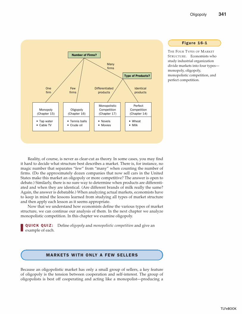
CHAPTER 16 OLIGOPOLY 351
Reality, of course, is never as clear-cut as theory. In some cases, you may findit hard to decide what structure best describes a market. There is, for instance, nomagic number that separates “few” from “many” when counting the number offirms. (Do the approximately dozen companies that now sell cars in the UnitedStates make this market an oligopoly or more competitive? The answer is open todebate.) Similarly, there is no sure way to determine when products are differenti-ated and when they are identical. (Are different brands of milk really the same?Again, the answer is debatable.) When analyzing actual markets, economists haveto keep in mind the lessons learned from studying all types of market structureand then apply each lesson as it seems appropriate.
Now that we understand how economists define the various types of marketstructure, we can continue our analysis of them. In the next chapter we analyzemonopolistic competition. In this chapter we examine oligopoly.
QUICK QUIZ: Define oligopoly and monopolistic competition and give an example of each.
MARKETS WITH ONLY A FEW SELLERS
Because an oligopolistic market has only a small group of sellers, a key featureof oligopoly is the tension between cooperation and self-interest. The group ofoligopolists is best off cooperating and acting like a monopolist—producing a
• Tap water• Cable TV
Monopoly(Chapter 15)
• Novels• Movies
• Wheat• Milk
MonopolisticCompetition(Chapter 17)
• Tennis balls• Crude oil
Oligopoly(Chapter 16)
Number of Firms?
PerfectCompetition(Chapter 14)
Type of Products?
Identicalproducts
Differentiatedproducts
Onefirm
Fewfirms
Manyfirms
Figure 16 -1
THE FOUR TYPES OF MARKET
STRUCTURE. Economists whostudy industrial organizationdivide markets into four types—monopoly, oligopoly,monopolistic competition, andperfect competition.
Oligopoly 341
TLFeBOOK
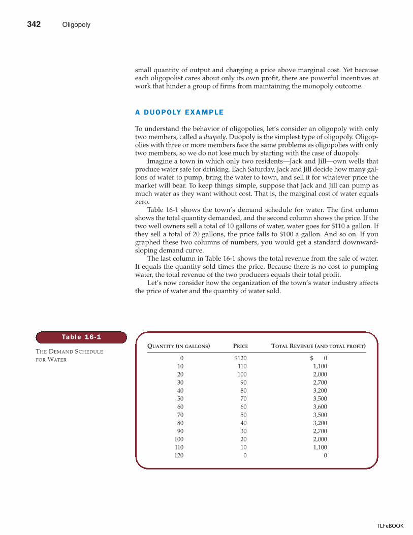
352 PART F IVE FIRM BEHAVIOR AND THE ORGANIZATION OF INDUSTRY
small quantity of output and charging a price above marginal cost. Yet becauseeach oligopolist cares about only its own profit, there are powerful incentives atwork that hinder a group of firms from maintaining the monopoly outcome.
A DUOPOLY EXAMPLE
To understand the behavior of oligopolies, let’s consider an oligopoly with onlytwo members, called a duopoly. Duopoly is the simplest type of oligopoly. Oligop-olies with three or more members face the same problems as oligopolies with onlytwo members, so we do not lose much by starting with the case of duopoly.
Imagine a town in which only two residents—Jack and Jill—own wells thatproduce water safe for drinking. Each Saturday, Jack and Jill decide how many gal-lons of water to pump, bring the water to town, and sell it for whatever price themarket will bear. To keep things simple, suppose that Jack and Jill can pump asmuch water as they want without cost. That is, the marginal cost of water equalszero.
Table 16-1 shows the town’s demand schedule for water. The first columnshows the total quantity demanded, and the second column shows the price. If thetwo well owners sell a total of 10 gallons of water, water goes for $110 a gallon. Ifthey sell a total of 20 gallons, the price falls to $100 a gallon. And so on. If yougraphed these two columns of numbers, you would get a standard downward-sloping demand curve.
The last column in Table 16-1 shows the total revenue from the sale of water.It equals the quantity sold times the price. Because there is no cost to pumpingwater, the total revenue of the two producers equals their total profit.
Let’s now consider how the organization of the town’s water industry affectsthe price of water and the quantity of water sold.
Table 16 -1
THE DEMAND SCHEDULE
FOR WATER
QUANTITY (IN GALLONS) PRICE TOTAL REVENUE (AND TOTAL PROFIT)
0 $120 $ 010 110 1,10020 100 2,00030 90 2,70040 80 3,20050 70 3,50060 60 3,60070 50 3,50080 40 3,20090 30 2,700
100 20 2,000110 10 1,100120 0 0
342 Oligopoly
TLFeBOOK
CHAPTER 16 OLIGOPOLY 353
COMPETIT ION, MONOPOLIES, AND CARTELS
Before considering the price and quantity of water that would result from theduopoly of Jack and Jill, let’s discuss briefly the two market structures we alreadyunderstand: competition and monopoly.
Consider first what would happen if the market for water were perfectlycompetitive. In a competitive market, the production decisions of each firm driveprice equal to marginal cost. In the market for water, marginal cost is zero. Thus,under competition, the equilibrium price of water would be zero, and the equi-librium quantity would be 120 gallons. The price of water would reflect the costof producing it, and the efficient quantity of water would be produced andconsumed.
Now consider how a monopoly would behave. Table 16-1 shows that totalprofit is maximized at a quantity of 60 gallons and a price of $60 a gallon. A profit-maximizing monopolist, therefore, would produce this quantity and charge thisprice. As is standard for monopolies, price would exceed marginal cost. The resultwould be inefficient, for the quantity of water produced and consumed would fallshort of the socially efficient level of 120 gallons.
What outcome should we expect from our duopolists? One possibility is thatJack and Jill get together and agree on the quantity of water to produce and theprice to charge for it. Such an agreement among firms over production and price iscalled collusion, and the group of firms acting in unison is called a cartel. Once acartel is formed, the market is in effect served by a monopoly, and we can applyour analysis from Chapter 15. That is, if Jack and Jill were to collude, they wouldagree on the monopoly outcome because that outcome maximizes the total profitthat the producers can get from the market. Our two producers would produce atotal of 60 gallons, which would be sold at a price of $60 a gallon. Once again, priceexceeds marginal cost, and the outcome is socially inefficient.
A cartel must agree not only on the total level of production but also on theamount produced by each member. In our case, Jack and Jill must agree how tosplit between themselves the monopoly production of 60 gallons. Each member ofthe cartel will want a larger share of the market because a larger market sharemeans larger profit. If Jack and Jill agreed to split the market equally, each wouldproduce 30 gallons, the price would be $60 a gallon, and each would get a profit of$1,800.
THE EQUIL IBRIUM FOR AN OLIGOPOLY
Although oligopolists would like to form cartels and earn monopoly profits, oftenthat is not possible. As we discuss later in this chapter, antitrust laws prohibit ex-plicit agreements among oligopolists as a matter of public policy. In addition,squabbling among cartel members over how to divide the profit in the marketsometimes makes agreement among them impossible. Let’s therefore considerwhat happens if Jack and Jill decide separately how much water to produce.
At first, one might expect Jack and Jill to reach the monopoly outcome on theirown, for this outcome maximizes their joint profit. In the absence of a bindingagreement, however, the monopoly outcome is unlikely. To see why, imagine thatJack expects Jill to produce only 30 gallons (half of the monopoly quantity). Jackwould reason as follows:
co l lus ionan agreement among firms in amarket about quantities to produceor prices to charge
car te la group of firms acting in unison
Oligopoly 343
TLFeBOOK
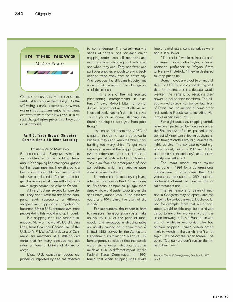
354 PART F IVE FIRM BEHAVIOR AND THE ORGANIZATION OF INDUSTRY
CARTELS ARE RARE, IN PART BECAUSE THE
antitrust laws make them illegal. As thefollowing article describes, however,ocean shipping firms enjoy an unusualexemption from these laws and, as a re-sult, charge higher prices than they oth-erwise would.
A s U . S . Tr a d e G r o w s , S h i p p i n gC a r t e l s G e t a B i t M o r e S c r u t i n y
BY ANNA WILDE MATTHEWS
RUTHERFORD, N.J.—Every two weeks, inan unobtrusive office building here,about 20 shipping-line managers gatherfor their usual meeting. They sit around along conference table, exchange smalltalk over bagels and coffee and then be-gin discussing what they will charge tomove cargo across the Atlantic Ocean.
All very routine, except for one de-tail: They don’t work for the same com-pany. Each represents a differentshipping line, supposedly competing forbusiness. Under U.S. antitrust law, mostpeople doing this would end up in court.
But shipping isn’t like other busi-nesses. Many of the world’s big shippinglines, from Sea-Land Service Inc. of theU.S. to A. P. Moller/Maersk Line of Den-mark, are members of a little-noticedcartel that for many decades has setrates on tens of billions of dollars ofcargo.
Most U.S. consumer goods ex-ported or imported by sea are affected
to some degree. The cartel—really aseries of cartels, one for each majorshipping route—can tell importers andexporters when shipping contracts startand when they end. They can favor oneport over another, enough to swing badlyneeded trade away from an entire city.And because the shipping industry hasan antitrust exemption from Congress,all of this is legal.
“This is one of the last legalizedprice-setting arrangements in exis-tence,” says Robert Litan, a formerJustice Department antitrust official. Air-lines and banks couldn’t do this, he says,“but if you’re an ocean shipping line,there’s nothing to stop you from pricefixing.”
You could call them the OPEC ofshipping, though not quite as powerfulbecause they can’t keep members frombuilding too many ships. To get morebusiness, some of the shipping cartels’own members undercut cartel rates ormake special deals with big customers.They also face the emergence of newcompetitors, which are keeping ratesdown in some markets.
Nonetheless, the industry is playinga bigger role now in the U.S. economyas American companies plunge moredeeply into world trade. Exports over theseas have jumped 26% in the past twoyears and 50% since the start of thedecade.
For consumers, the impact is hardto measure. Transportation costs makeup 5% to 10% of the price of mostgoods, and increases in shipping ratesare usually passed on to consumers. Alimited 1993 survey by the AgricultureDepartment, examining $5 billion of U.S.farm exports, concluded that the cartelswere raising ocean shipping rates asmuch as 18%. A different report, by theFederal Trade Commission in 1995,found that when shipping lines broke
free of cartel rates, contract prices wereabout 19% lower.
“The cartels’ whole makeup is anti-consumer,” says John Taylor, a trans-portation professor at Wayne StateUniversity in Detroit. “They’re designedto keep prices up.”
Some moves are afoot to change allthis. The U.S. Senate is considering a billthat, for the first time in a decade, wouldweaken the cartels, by reducing theirpower to police their members. The bill,sponsored by Sen. Kay Bailey Hutchisonof Texas, has the support of some otherhigh-ranking Republicans, including Ma-jority Leader Trent Lott. . . .
For eight decades, shipping cartelshave been protected by Congress underthe Shipping Act of 1916, passed at thebehest of American shipping customers,who thought cartels would guarantee re-liable service. The law was revised sig-nificantly only twice, in 1961 and 1984,but both times the industry’s antitrust im-munity was left intact.
The most recent major reviewwas done in 1991 by a congressionalcommission. It heard more than 100witnesses, produced a 250-page re-port—and offered no conclusions orrecommendations. . . .
The real reasons for years of inac-tion in Congress may be apathy and thelobbying by various groups. Dockside la-bor, for example, fears that secret con-tracts would enable ship lines to divertcargo to nonunion workers without theunion knowing it. David Butz, a Univer-sity of Michigan economist who hasstudied shipping, thinks voters aren’tlikely to weigh in; the cartels aren’t a hottopic. “It’s below the radar screen,” hesays. “Consumers don’t realize the im-pact they have.”
SOURCE: The Wall Street Journal, October 7, 1997,p. A1.
IN THE NEWS
Modern Pirates
344 Oligopoly
TLFeBOOK
CHAPTER 16 OLIGOPOLY 355
“I could produce 30 gallons as well. In this case, a total of 60 gallons of waterwould be sold at a price of $60 a gallon. My profit would be $1,800 (30 gallons �$60 a gallon). Alternatively, I could produce 40 gallons. In this case, a total of 70gallons of water would be sold at a price of $50 a gallon. My profit would be $2,000(40 gallons � $50 a gallon). Even though total profit in the market would fall, myprofit would be higher, because I would have a larger share of the market.”
Of course, Jill might reason the same way. If so, Jack and Jill would each bring40 gallons to town. Total sales would be 80 gallons, and the price would fall to $40.Thus, if the duopolists individually pursue their own self-interest when decidinghow much to produce, they produce a total quantity greater than the monopolyquantity, charge a price lower than the monopoly price, and earn total profit lessthan the monopoly profit.
Although the logic of self-interest increases the duopoly’s output above themonopoly level, it does not push the duopolists to reach the competitive alloca-tion. Consider what happens when each duopolist is producing 40 gallons. Theprice is $40, and each duopolist makes a profit of $1,600. In this case, Jack’s self-interested logic leads to a different conclusion:
“Right now, my profit is $1,600. Suppose I increase my production to 50 gallons.In this case, a total of 90 gallons of water would be sold, and the price would be $30a gallon. Then my profit would be only $1,500. Rather than increasing productionand driving down the price, I am better off keeping my production at 40 gallons.”
The outcome in which Jack and Jill each produce 40 gallons looks like some sortof equilibrium. In fact, this outcome is called a Nash equilibrium (named after eco-nomic theorist John Nash). A Nash equilibrium is a situation in which economicactors interacting with one another each choose their best strategy given the strate-gies the others have chosen. In this case, given that Jill is producing 40 gallons, thebest strategy for Jack is to produce 40 gallons. Similarly, given that Jack is produc-ing 40 gallons, the best strategy for Jill is to produce 40 gallons. Once they reach thisNash equilibrium, neither Jack nor Jill has an incentive to make a different decision.
This example illustrates the tension between cooperation and self-interest. Oli-gopolists would be better off cooperating and reaching the monopoly outcome. Yetbecause they pursue their own self-interest, they do not end up reaching the mo-nopoly outcome and maximizing their joint profit. Each oligopolist is tempted toraise production and capture a larger share of the market. As each of them tries todo this, total production rises, and the price falls.
At the same time, self-interest does not drive the market all the way to thecompetitive outcome. Like monopolists, oligopolists are aware that increases inthe amount they produce reduce the price of their product. Therefore, they stopshort of following the competitive firm’s rule of producing up to the point whereprice equals marginal cost.
In summary, when firms in an oligopoly individually choose production to maximizeprofit, they produce a quantity of output greater than the level produced by monopoly andless than the level produced by competition. The oligopoly price is less than the monopolyprice but greater than the competitive price (which equals marginal cost).
HOW THE SIZE OF AN OLIGOPOLYAFFECTS THE MARKET OUTCOME
We can use the insights from this analysis of duopoly to discuss how the size of anoligopoly is likely to affect the outcome in a market. Suppose, for instance, that
Nash equ i l ib r iuma situation in which economic actorsinteracting with one another eachchoose their best strategy given thestrategies that all the other actorshave chosen
Oligopoly 345
TLFeBOOK
356 PART F IVE FIRM BEHAVIOR AND THE ORGANIZATION OF INDUSTRY
John and Joan suddenly discover water sources on their property and join Jack andJill in the water oligopoly. The demand schedule in Table 16-1 remains the same,but now more producers are available to satisfy this demand. How would an in-crease in the number of sellers from two to four affect the price and quantity of wa-ter in the town?
If the sellers of water could form a cartel, they would once again try to maxi-mize total profit by producing the monopoly quantity and charging the monopolyprice. Just as when there were only two sellers, the members of the cartel wouldneed to agree on production levels for each member and find some way to enforcethe agreement. As the cartel grows larger, however, this outcome is less likely.Reaching and enforcing an agreement becomes more difficult as the size of thegroup increases.
If the oligopolists do not form a cartel—perhaps because the antitrust lawsprohibit it—they must each decide on their own how much water to produce. Tosee how the increase in the number of sellers affects the outcome, consider the de-cision facing each seller. At any time, each well owner has the option to raise pro-duction by 1 gallon. In making this decision, the well owner weighs two effects:
� The output effect: Because price is above marginal cost, selling 1 more gallonof water at the going price will raise profit.
� The price effect: Raising production will increase the total amount sold, whichwill lower the price of water and lower the profit on all the other gallonssold.
If the output effect is larger than the price effect, the well owner will increase pro-duction. If the price effect is larger than the output effect, the owner will not raiseproduction. (In fact, in this case, it is profitable to reduce production.) Each oli-gopolist continues to increase production until these two marginal effects exactlybalance, taking the other firms’ production as given.
Now consider how the number of firms in the industry affects the marginalanalysis of each oligopolist. The larger the number of sellers, the less concernedeach seller is about its own impact on the market price. That is, as the oligopolygrows in size, the magnitude of the price effect falls. When the oligopoly growsvery large, the price effect disappears altogether, leaving only the output effect. Inthis extreme case, each firm in the oligopoly increases production as long as priceis above marginal cost.
We can now see that a large oligopoly is essentially a group of competitivefirms. A competitive firm considers only the output effect when deciding howmuch to produce: Because a competitive firm is a price taker, the price effect is ab-sent. Thus, as the number of sellers in an oligopoly grows larger, an oligopolistic marketlooks more and more like a competitive market. The price approaches marginal cost, and thequantity produced approaches the socially efficient level.
This analysis of oligopoly offers a new perspective on the effects of interna-tional trade. Imagine that Toyota and Honda are the only automakers in Japan,Volkswagen and Mercedes-Benz are the only automakers in Germany, and Fordand General Motors are the only automakers in the United States. If these nationsprohibited trade in autos, each would have an auto oligopoly with only two mem-bers, and the market outcome would likely depart substantially from the compet-itive ideal. With international trade, however, the car market is a world market,and the oligopoly in this example has six members. Allowing free trade increases
346 Oligopoly
TLFeBOOK
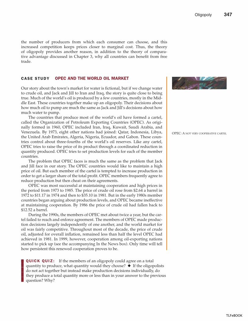
CHAPTER 16 OLIGOPOLY 357
CASE STUDY OPEC AND THE WORLD OIL MARKET
Our story about the town’s market for water is fictional, but if we change waterto crude oil, and Jack and Jill to Iran and Iraq, the story is quite close to beingtrue. Much of the world’s oil is produced by a few countries, mostly in the Mid-dle East. These countries together make up an oligopoly. Their decisions abouthow much oil to pump are much the same as Jack and Jill’s decisions about howmuch water to pump.
The countries that produce most of the world’s oil have formed a cartel,called the Organization of Petroleum Exporting Countries (OPEC). As origi-nally formed in 1960, OPEC included Iran, Iraq, Kuwait, Saudi Arabia, andVenezuela. By 1973, eight other nations had joined: Qatar, Indonesia, Libya,the United Arab Emirates, Algeria, Nigeria, Ecuador, and Gabon. These coun-tries control about three-fourths of the world’s oil reserves. Like any cartel,OPEC tries to raise the price of its product through a coordinated reduction inquantity produced. OPEC tries to set production levels for each of the membercountries.
The problem that OPEC faces is much the same as the problem that Jackand Jill face in our story. The OPEC countries would like to maintain a highprice of oil. But each member of the cartel is tempted to increase production inorder to get a larger share of the total profit. OPEC members frequently agree toreduce production but then cheat on their agreements.
OPEC was most successful at maintaining cooperation and high prices inthe period from 1973 to 1985. The price of crude oil rose from $2.64 a barrel in1972 to $11.17 in 1974 and then to $35.10 in 1981. But in the early 1980s membercountries began arguing about production levels, and OPEC became ineffectiveat maintaining cooperation. By 1986 the price of crude oil had fallen back to$12.52 a barrel.
During the 1990s, the members of OPEC met about twice a year, but the car-tel failed to reach and enforce agreement. The members of OPEC made produc-tion decisions largely independently of one another, and the world market foroil was fairly competitive. Throughout most of the decade, the price of crudeoil, adjusted for overall inflation, remained less than half the level OPEC hadachieved in 1981. In 1999, however, cooperation among oil-exporting nationsstarted to pick up (see the accompanying In the News box). Only time will tellhow persistent this renewed cooperation proves to be.
the number of producers from which each consumer can choose, and thisincreased competition keeps prices closer to marginal cost. Thus, the theoryof oligopoly provides another reason, in addition to the theory of compara-tive advantage discussed in Chapter 3, why all countries can benefit from freetrade.
OPEC: A NOT VERY COOPERATIVE CARTEL
QUICK QUIZ: If the members of an oligopoly could agree on a total quantity to produce, what quantity would they choose? � If the oligopolists do not act together but instead make production decisions individually, do they produce a total quantity more or less than in your answer to the previous question? Why?
Oligopoly 347
TLFeBOOK
358 PART F IVE FIRM BEHAVIOR AND THE ORGANIZATION OF INDUSTRY
GAME THEORY AND THEECONOMICS OF COOPERATION
As we have seen, oligopolies would like to reach the monopoly outcome, but do-ing so requires cooperation, which at times is difficult to maintain. In this sectionwe look more closely at the problems people face when cooperation is desirablebut difficult. To analyze the economics of cooperation, we need to learn a littleabout game theory.
Game theory is the study of how people behave in strategic situations. By“strategic” we mean a situation in which each person, when deciding what actionsto take, must consider how others might respond to that action. Because the num-ber of firms in an oligopolistic market is small, each firm must act strategically.Each firm knows that its profit depends not only on how much it produces butalso on how much the other firms produce. In making its production decision,each firm in an oligopoly should consider how its decision might affect the pro-duction decisions of all the other firms.
Game theory is not necessary for understanding competitive or monopolymarkets. In a competitive market, each firm is so small compared to the marketthat strategic interactions with other firms are not important. In a monopolizedmarket, strategic interactions are absent because the market has only one firm. But,as we will see, game theory is quite useful for understanding the behavior ofoligopolies.
OPEC FAILED TO KEEP OIL PRICES HIGH
during most of the 1990s, but thisstarted to change in 1999.
A n O i l O u t s i d e r R e v i v e s a C a r t e l
BY AGIS SALPUKAS
The price of crude oil has doubled sinceearly last year. Higher prices for gaso-
line, heating oil, and other products arehitting every consumer’s pocketbook.
Is OPEC flexing its muscle again?Not exactly. There’s a new cartel in town,and after a shaky start two years ago, itsmembers have achieved—for now, atleast—the unity necessary to hold totheir production quotas. And that meanshigher prices.
In a sense, this cartel is simply the11 members of the Organization of Pe-troleum Exporting Countries plus two—Mexico and Norway. But the world’soil-producing and exporting nations arewielding power this time around mainlybecause of a shove not from the MiddleEast but rather from Mexico—and espe-cially from its persistent energy minister,Luis K. Tellez. . . . Already, the price of
crude oil has more than doubled, to$23.45 a barrel from $11 early this year.
Not that the coalition is home free.Prices hit $24 a barrel last month, butslipped back when traders thought theysaw hints of cracks in the cartel’s soli-darity. After all, if one country breaksranks, the cartel’s tenuous grip on theworld market could crumble.
For the moment, though, thereseems little easing in the cartel’s unitedfront or in rising oil prices.
SOURCE: The New York Times, Money & BusinessSection, October 24, 1999, p. 1.
IN THE NEWS
The Oil CartelMakes a Comeback
game theor ythe study of how people behave instrategic situations
348 Oligopoly
TLFeBOOK
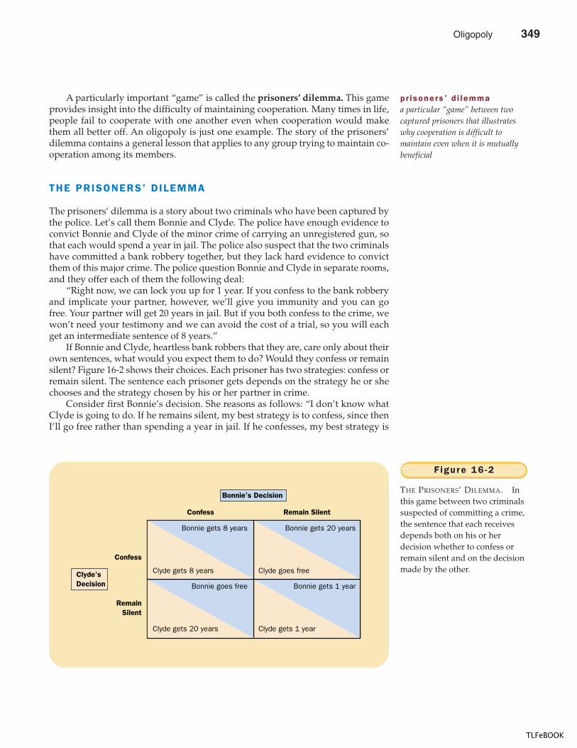
CHAPTER 16 OLIGOPOLY 359
A particularly important “game” is called the prisoners’ dilemma. This gameprovides insight into the difficulty of maintaining cooperation. Many times in life,people fail to cooperate with one another even when cooperation would makethem all better off. An oligopoly is just one example. The story of the prisoners’dilemma contains a general lesson that applies to any group trying to maintain co-operation among its members.
THE PRISONERS’ DILEMMA
The prisoners’ dilemma is a story about two criminals who have been captured bythe police. Let’s call them Bonnie and Clyde. The police have enough evidence toconvict Bonnie and Clyde of the minor crime of carrying an unregistered gun, sothat each would spend a year in jail. The police also suspect that the two criminalshave committed a bank robbery together, but they lack hard evidence to convictthem of this major crime. The police question Bonnie and Clyde in separate rooms,and they offer each of them the following deal:
“Right now, we can lock you up for 1 year. If you confess to the bank robberyand implicate your partner, however, we’ll give you immunity and you can gofree. Your partner will get 20 years in jail. But if you both confess to the crime, wewon’t need your testimony and we can avoid the cost of a trial, so you will eachget an intermediate sentence of 8 years.”
If Bonnie and Clyde, heartless bank robbers that they are, care only about theirown sentences, what would you expect them to do? Would they confess or remainsilent? Figure 16-2 shows their choices. Each prisoner has two strategies: confess orremain silent. The sentence each prisoner gets depends on the strategy he or shechooses and the strategy chosen by his or her partner in crime.
Consider first Bonnie’s decision. She reasons as follows: “I don’t know whatClyde is going to do. If he remains silent, my best strategy is to confess, since thenI’ll go free rather than spending a year in jail. If he confesses, my best strategy is
pr isoners ’ d i lemmaa particular “game” between twocaptured prisoners that illustrateswhy cooperation is difficult tomaintain even when it is mutuallybeneficial
Bonnie’s Decision
Confess
Confess
Bonnie gets 8 years
Clyde gets 8 years
Bonnie gets 20 years
Clyde goes free
Bonnie goes free
Clyde gets 20 years
Bonnie gets 1 year
Clyde gets 1 year
Remain Silent
RemainSilent
Clyde’sDecision
F igure 16 -2
THE PRISONERS’ DILEMMA. Inthis game between two criminalssuspected of committing a crime,the sentence that each receivesdepends both on his or herdecision whether to confess orremain silent and on the decisionmade by the other.
Oligopoly 349
TLFeBOOK
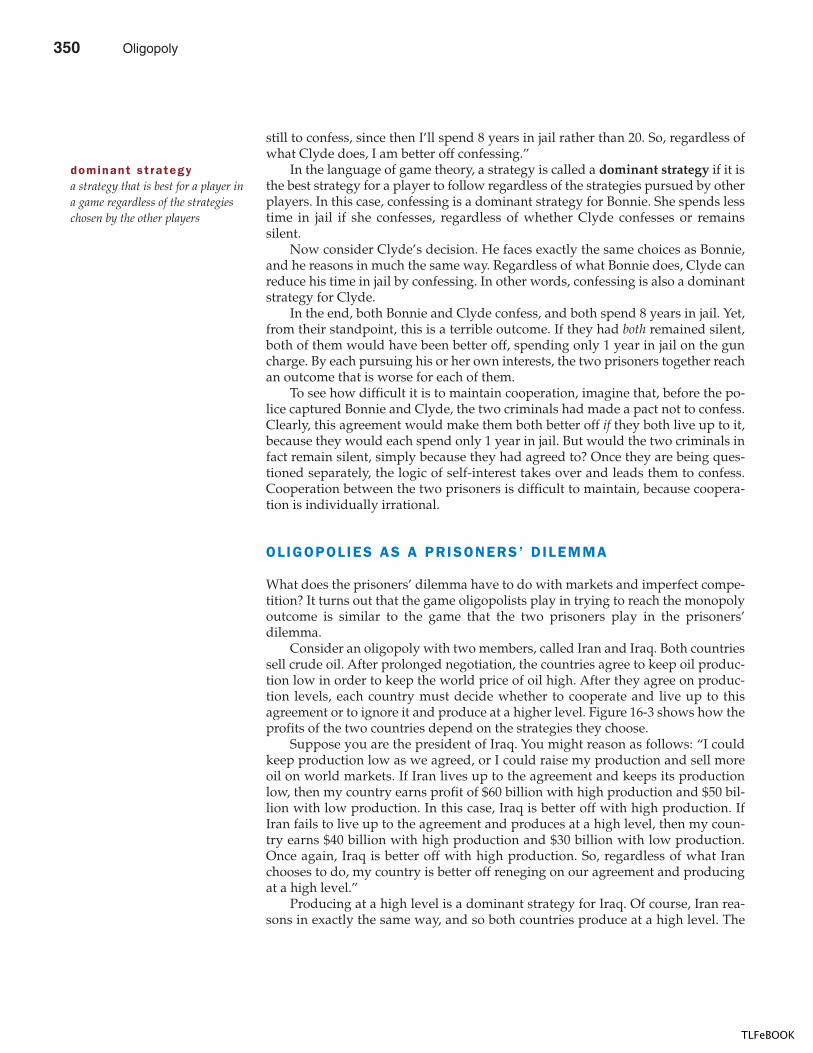
360 PART F IVE FIRM BEHAVIOR AND THE ORGANIZATION OF INDUSTRY
still to confess, since then I’ll spend 8 years in jail rather than 20. So, regardless ofwhat Clyde does, I am better off confessing.”
In the language of game theory, a strategy is called a dominant strategy if it isthe best strategy for a player to follow regardless of the strategies pursued by otherplayers. In this case, confessing is a dominant strategy for Bonnie. She spends lesstime in jail if she confesses, regardless of whether Clyde confesses or remainssilent.
Now consider Clyde’s decision. He faces exactly the same choices as Bonnie,and he reasons in much the same way. Regardless of what Bonnie does, Clyde canreduce his time in jail by confessing. In other words, confessing is also a dominantstrategy for Clyde.
In the end, both Bonnie and Clyde confess, and both spend 8 years in jail. Yet,from their standpoint, this is a terrible outcome. If they had both remained silent,both of them would have been better off, spending only 1 year in jail on the guncharge. By each pursuing his or her own interests, the two prisoners together reachan outcome that is worse for each of them.
To see how difficult it is to maintain cooperation, imagine that, before the po-lice captured Bonnie and Clyde, the two criminals had made a pact not to confess.Clearly, this agreement would make them both better off if they both live up to it,because they would each spend only 1 year in jail. But would the two criminals infact remain silent, simply because they had agreed to? Once they are being ques-tioned separately, the logic of self-interest takes over and leads them to confess.Cooperation between the two prisoners is difficult to maintain, because coopera-tion is individually irrational.
OLIGOPOLIES AS A PRISONERS’ DILEMMA
What does the prisoners’ dilemma have to do with markets and imperfect compe-tition? It turns out that the game oligopolists play in trying to reach the monopolyoutcome is similar to the game that the two prisoners play in the prisoners’dilemma.
Consider an oligopoly with two members, called Iran and Iraq. Both countriessell crude oil. After prolonged negotiation, the countries agree to keep oil produc-tion low in order to keep the world price of oil high. After they agree on produc-tion levels, each country must decide whether to cooperate and live up to thisagreement or to ignore it and produce at a higher level. Figure 16-3 shows how theprofits of the two countries depend on the strategies they choose.
Suppose you are the president of Iraq. You might reason as follows: “I couldkeep production low as we agreed, or I could raise my production and sell moreoil on world markets. If Iran lives up to the agreement and keeps its productionlow, then my country earns profit of $60 billion with high production and $50 bil-lion with low production. In this case, Iraq is better off with high production. IfIran fails to live up to the agreement and produces at a high level, then my coun-try earns $40 billion with high production and $30 billion with low production.Once again, Iraq is better off with high production. So, regardless of what Iranchooses to do, my country is better off reneging on our agreement and producingat a high level.”
Producing at a high level is a dominant strategy for Iraq. Of course, Iran rea-sons in exactly the same way, and so both countries produce at a high level. The
dominant st rategya strategy that is best for a player ina game regardless of the strategieschosen by the other players
350 Oligopoly
TLFeBOOK
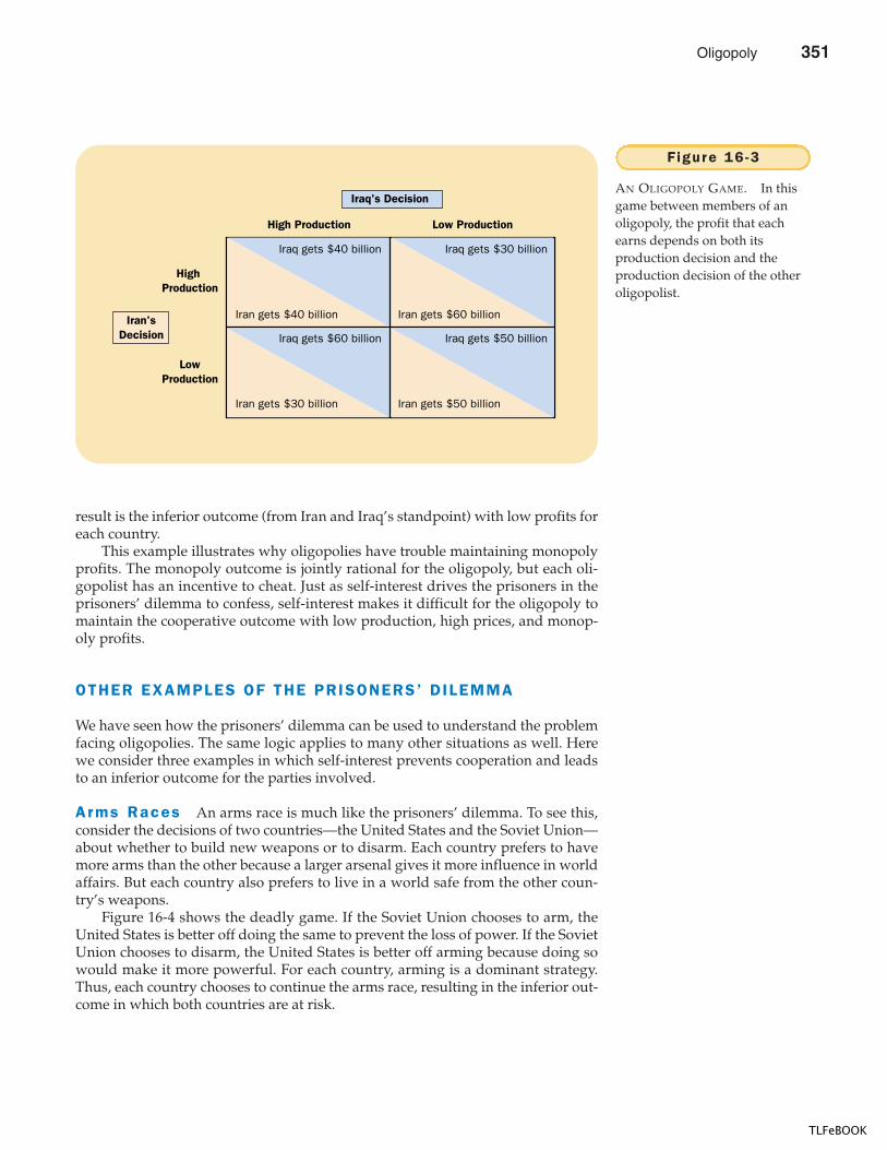
CHAPTER 16 OLIGOPOLY 361
result is the inferior outcome (from Iran and Iraq’s standpoint) with low profits foreach country.
This example illustrates why oligopolies have trouble maintaining monopolyprofits. The monopoly outcome is jointly rational for the oligopoly, but each oli-gopolist has an incentive to cheat. Just as self-interest drives the prisoners in theprisoners’ dilemma to confess, self-interest makes it difficult for the oligopoly tomaintain the cooperative outcome with low production, high prices, and monop-oly profits.
OTHER EXAMPLES OF THE PRISONERS’ DILEMMA
We have seen how the prisoners’ dilemma can be used to understand the problemfacing oligopolies. The same logic applies to many other situations as well. Herewe consider three examples in which self-interest prevents cooperation and leadsto an inferior outcome for the parties involved.
Arms Races An arms race is much like the prisoners’ dilemma. To see this,consider the decisions of two countries—the United States and the Soviet Union—about whether to build new weapons or to disarm. Each country prefers to havemore arms than the other because a larger arsenal gives it more influence in worldaffairs. But each country also prefers to live in a world safe from the other coun-try’s weapons.
Figure 16-4 shows the deadly game. If the Soviet Union chooses to arm, theUnited States is better off doing the same to prevent the loss of power. If the SovietUnion chooses to disarm, the United States is better off arming because doing sowould make it more powerful. For each country, arming is a dominant strategy.Thus, each country chooses to continue the arms race, resulting in the inferior out-come in which both countries are at risk.
Iraq's Decision
High Production
High Production
Iraq gets $40 billion
Iran gets $40 billion
Iraq gets $30 billion
Iran gets $60 billion
Iraq gets $60 billion
Iran gets $30 billion
Iraq gets $50 billion
Iran gets $50 billion
Low Production
LowProduction
Iran'sDecision
F igure 16 -3
AN OLIGOPOLY GAME. In thisgame between members of anoligopoly, the profit that eachearns depends on both itsproduction decision and theproduction decision of the otheroligopolist.
Oligopoly 351
TLFeBOOK
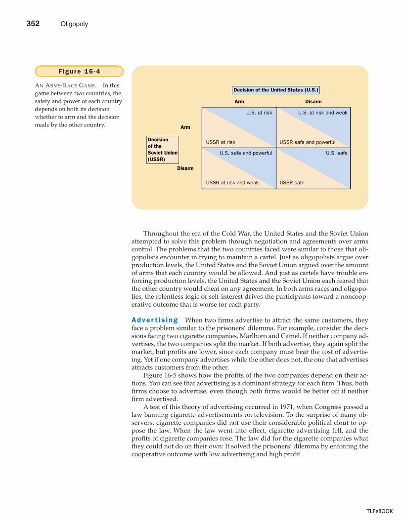
362 PART F IVE FIRM BEHAVIOR AND THE ORGANIZATION OF INDUSTRY
Throughout the era of the Cold War, the United States and the Soviet Unionattempted to solve this problem through negotiation and agreements over armscontrol. The problems that the two countries faced were similar to those that oli-gopolists encounter in trying to maintain a cartel. Just as oligopolists argue overproduction levels, the United States and the Soviet Union argued over the amountof arms that each country would be allowed. And just as cartels have trouble en-forcing production levels, the United States and the Soviet Union each feared thatthe other country would cheat on any agreement. In both arms races and oligopo-lies, the relentless logic of self-interest drives the participants toward a noncoop-erative outcome that is worse for each party.
Adver t i s ing When two firms advertise to attract the same customers, theyface a problem similar to the prisoners’ dilemma. For example, consider the deci-sions facing two cigarette companies, Marlboro and Camel. If neither company ad-vertises, the two companies split the market. If both advertise, they again split themarket, but profits are lower, since each company must bear the cost of advertis-ing. Yet if one company advertises while the other does not, the one that advertisesattracts customers from the other.
Figure 16-5 shows how the profits of the two companies depend on their ac-tions. You can see that advertising is a dominant strategy for each firm. Thus, bothfirms choose to advertise, even though both firms would be better off if neitherfirm advertised.
A test of this theory of advertising occurred in 1971, when Congress passed alaw banning cigarette advertisements on television. To the surprise of many ob-servers, cigarette companies did not use their considerable political clout to op-pose the law. When the law went into effect, cigarette advertising fell, and theprofits of cigarette companies rose. The law did for the cigarette companies whatthey could not do on their own: It solved the prisoners’ dilemma by enforcing thecooperative outcome with low advertising and high profit.
Decision of the United States (U.S.)
Arm
Arm
U.S. at risk
USSR at risk
U.S. at risk and weak
USSR safe and powerful
U.S. safe and powerful
USSR at risk and weak
U.S. safe
USSR safe
Disarm
Disarm
Decision of the Soviet Union (USSR)
F igure 16 -4
AN ARMS-RACE GAME. In thisgame between two countries, thesafety and power of each countrydepends on both its decisionwhether to arm and the decisionmade by the other country.
352 Oligopoly
TLFeBOOK
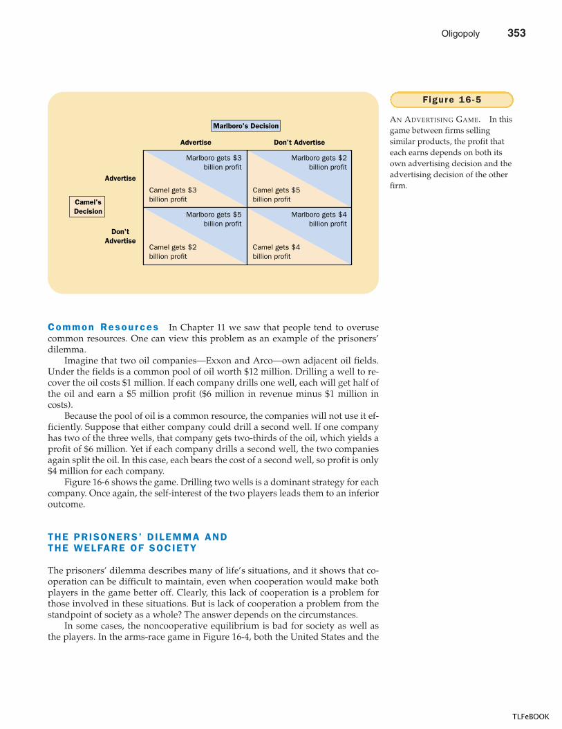
CHAPTER 16 OLIGOPOLY 363
Common Resources In Chapter 11 we saw that people tend to overusecommon resources. One can view this problem as an example of the prisoners’dilemma.
Imagine that two oil companies—Exxon and Arco—own adjacent oil fields.Under the fields is a common pool of oil worth $12 million. Drilling a well to re-cover the oil costs $1 million. If each company drills one well, each will get half ofthe oil and earn a $5 million profit ($6 million in revenue minus $1 million incosts).
Because the pool of oil is a common resource, the companies will not use it ef-ficiently. Suppose that either company could drill a second well. If one companyhas two of the three wells, that company gets two-thirds of the oil, which yields aprofit of $6 million. Yet if each company drills a second well, the two companiesagain split the oil. In this case, each bears the cost of a second well, so profit is only$4 million for each company.
Figure 16-6 shows the game. Drilling two wells is a dominant strategy for eachcompany. Once again, the self-interest of the two players leads them to an inferioroutcome.
THE PRISONERS’ DILEMMA ANDTHE WELFARE OF SOCIETY
The prisoners’ dilemma describes many of life’s situations, and it shows that co-operation can be difficult to maintain, even when cooperation would make bothplayers in the game better off. Clearly, this lack of cooperation is a problem forthose involved in these situations. But is lack of cooperation a problem from thestandpoint of society as a whole? The answer depends on the circumstances.
In some cases, the noncooperative equilibrium is bad for society as well asthe players. In the arms-race game in Figure 16-4, both the United States and the
Marlboro's Decision
Advertise
Advertise
Marlboro gets $3billion profit
Camel gets $3billion profit
Camel gets $5billion profit
Camel gets $2billion profit
Camel gets $4billion profit
Marlboro gets $2billion profit
Marlboro gets $5billion profit
Marlboro gets $4billion profit
Don't Advertise
Don'tAdvertise
Camel'sDecision
F igure 16 -5
AN ADVERTISING GAME. In thisgame between firms sellingsimilar products, the profit thateach earns depends on both itsown advertising decision and theadvertising decision of the otherfirm.
Oligopoly 353
TLFeBOOK
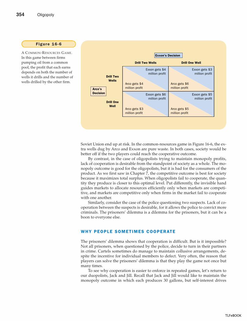
364 PART F IVE FIRM BEHAVIOR AND THE ORGANIZATION OF INDUSTRY
Soviet Union end up at risk. In the common-resources game in Figure 16-6, the ex-tra wells dug by Arco and Exxon are pure waste. In both cases, society would bebetter off if the two players could reach the cooperative outcome.
By contrast, in the case of oligopolists trying to maintain monopoly profits,lack of cooperation is desirable from the standpoint of society as a whole. The mo-nopoly outcome is good for the oligopolists, but it is bad for the consumers of theproduct. As we first saw in Chapter 7, the competitive outcome is best for societybecause it maximizes total surplus. When oligopolists fail to cooperate, the quan-tity they produce is closer to this optimal level. Put differently, the invisible handguides markets to allocate resources efficiently only when markets are competi-tive, and markets are competitive only when firms in the market fail to cooperatewith one another.
Similarly, consider the case of the police questioning two suspects. Lack of co-operation between the suspects is desirable, for it allows the police to convict morecriminals. The prisoners’ dilemma is a dilemma for the prisoners, but it can be aboon to everyone else.
WHY PEOPLE SOMETIMES COOPERATE
The prisoners’ dilemma shows that cooperation is difficult. But is it impossible?Not all prisoners, when questioned by the police, decide to turn in their partnersin crime. Cartels sometimes do manage to maintain collusive arrangements, de-spite the incentive for individual members to defect. Very often, the reason thatplayers can solve the prisoners’ dilemma is that they play the game not once butmany times.
To see why cooperation is easier to enforce in repeated games, let’s return toour duopolists, Jack and Jill. Recall that Jack and Jill would like to maintain themonopoly outcome in which each produces 30 gallons, but self-interest drives
Exxon's Decision
Drill TwoWells
Drill Two Wells
Exxon gets $4million profit
Arco gets $4million profit
Arco gets $6million profit
Arco gets $3million profit
Arco gets $5million profit
Exxon gets $3million profit
Exxon gets $6million profit
Exxon gets $5million profit
Drill One Well
Drill OneWell
Arco'sDecision
F igure 16 -6
A COMMON-RESOURCES GAME.In this game between firmspumping oil from a commonpool, the profit that each earnsdepends on both the number ofwells it drills and the number ofwells drilled by the other firm.
354 Oligopoly
TLFeBOOK
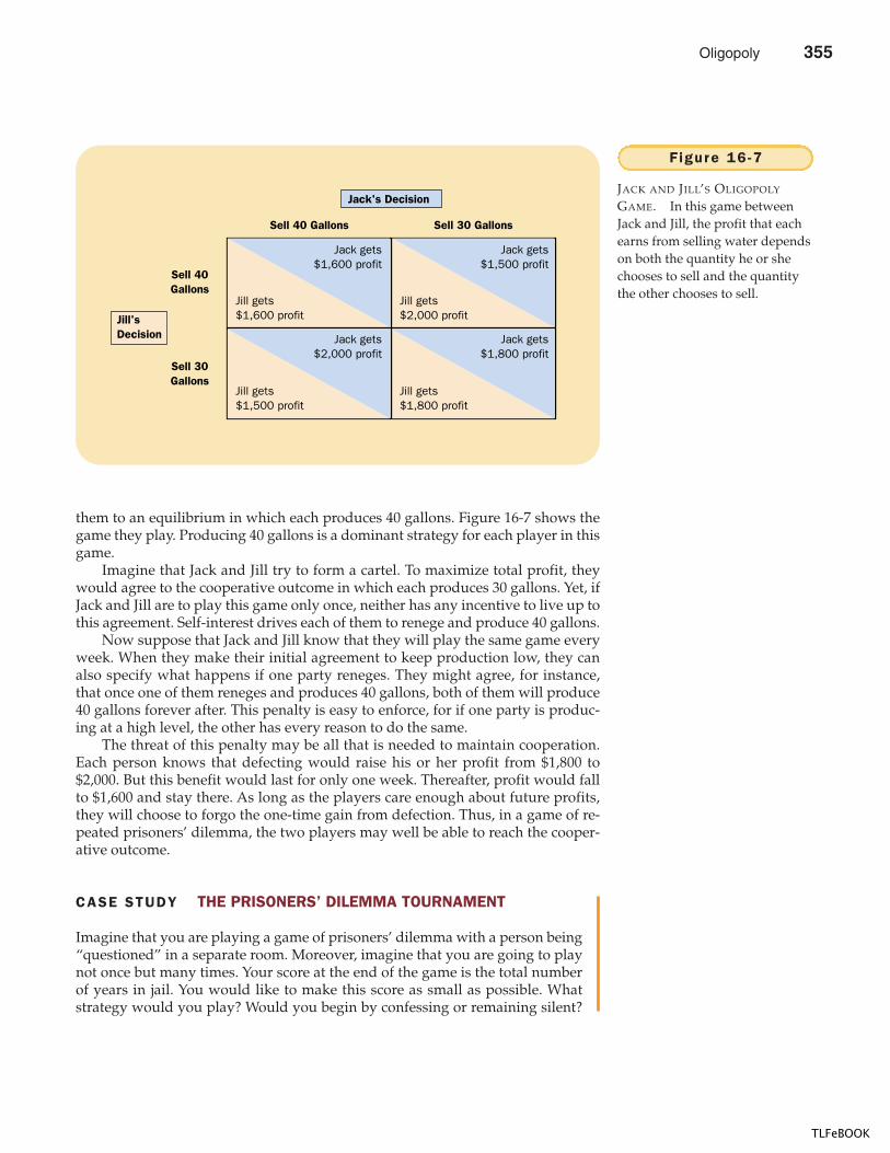
CHAPTER 16 OLIGOPOLY 365
CASE STUDY THE PRISONERS’ DILEMMA TOURNAMENT
Imagine that you are playing a game of prisoners’ dilemma with a person being“questioned” in a separate room. Moreover, imagine that you are going to playnot once but many times. Your score at the end of the game is the total numberof years in jail. You would like to make this score as small as possible. Whatstrategy would you play? Would you begin by confessing or remaining silent?
them to an equilibrium in which each produces 40 gallons. Figure 16-7 shows thegame they play. Producing 40 gallons is a dominant strategy for each player in thisgame.
Imagine that Jack and Jill try to form a cartel. To maximize total profit, theywould agree to the cooperative outcome in which each produces 30 gallons. Yet, ifJack and Jill are to play this game only once, neither has any incentive to live up tothis agreement. Self-interest drives each of them to renege and produce 40 gallons.
Now suppose that Jack and Jill know that they will play the same game everyweek. When they make their initial agreement to keep production low, they canalso specify what happens if one party reneges. They might agree, for instance,that once one of them reneges and produces 40 gallons, both of them will produce40 gallons forever after. This penalty is easy to enforce, for if one party is produc-ing at a high level, the other has every reason to do the same.
The threat of this penalty may be all that is needed to maintain cooperation.Each person knows that defecting would raise his or her profit from $1,800 to$2,000. But this benefit would last for only one week. Thereafter, profit would fallto $1,600 and stay there. As long as the players care enough about future profits,they will choose to forgo the one-time gain from defection. Thus, in a game of re-peated prisoners’ dilemma, the two players may well be able to reach the cooper-ative outcome.
Jack's Decision
Sell 40Gallons
Sell 40 Gallons
Jack gets$1,600 profit
Jill gets$1,600 profit
Jill gets$2,000 profit
Jill gets$1,500 profit
Jill gets$1,800 profit
Jack gets$1,500 profit
Jack gets$2,000 profit
Jack gets$1,800 profit
Sell 30 Gallons
Sell 30Gallons
Jill'sDecision
F igure 16 -7
JACK AND JILL’S OLIGOPOLY
GAME. In this game betweenJack and Jill, the profit that eachearns from selling water dependson both the quantity he or shechooses to sell and the quantitythe other chooses to sell.
Oligopoly 355
TLFeBOOK
366 PART F IVE FIRM BEHAVIOR AND THE ORGANIZATION OF INDUSTRY
How would the other player’s actions affect your subsequent decisions aboutconfessing?
Repeated prisoners’ dilemma is quite a complicated game. To encouragecooperation, players must penalize each other for not cooperating. Yet the strat-egy described earlier for Jack and Jill’s water cartel—defect forever as soon asthe other player defects—is not very forgiving. In a game repeated many times,a strategy that allows players to return to the cooperative outcome after a pe-riod of noncooperation may be preferable.
To see what strategies work best, political scientist Robert Axelrod held atournament. People entered by sending computer programs designed to playrepeated prisoners’ dilemma. Each program then played the game against allthe other programs. The “winner” was the program that received the fewesttotal years in jail.
The winner turned out to be a simple strategy called tit-for-tat. According totit-for-tat, a player should start by cooperating and then do whatever the otherplayer did last time. Thus, a tit-for-tat player cooperates until the other playerdefects; he then defects until the other player cooperates again. In other words,this strategy starts out friendly, penalizes unfriendly players, and forgives themif warranted. To Axelrod’s surprise, this simple strategy did better than all themore complicated strategies that people had sent in.
The tit-for-tat strategy has a long history. It is essentially the biblical strat-egy of “an eye for an eye, a tooth for a tooth.” The prisoners’ dilemma tourna-ment suggests that this may be a good rule of thumb for playing some of thegames of life.
QUICK QUIZ: Tell the story of the prisoners’ dilemma. Write down a table showing the prisoners’ choices and explain what outcome is likely. � What does the prisoners’ dilemma teach us about oligopolies?
PUBLIC POLICY TOWARD OLIGOPOLIES
One of the Ten Principles of Economics in Chapter 1 is that governments can some-times improve market outcomes. The application of this principle to oligopolisticmarkets is, as a general matter, straightforward. As we have seen, cooperationamong oligopolists is undesirable from the standpoint of society as a whole, be-cause it leads to production that is too low and prices that are too high. To movethe allocation of resources closer to the social optimum, policymakers should tryto induce firms in an oligopoly to compete rather than cooperate. Let’s considerhow policymakers do this and then examine the controversies that arise in thisarea of public policy.
RESTRAINT OF TRADE AND THE ANTITRUST LAWS
One way that policy discourages cooperation is through the common law. Nor-mally, freedom of contract is an essential part of a market economy. Businesses andhouseholds use contracts to arrange mutually advantageous trades. In doing this,
356 Oligopoly
TLFeBOOK
CHAPTER 16 OLIGOPOLY 367
CASE STUDY AN ILLEGAL PHONE CALL
Firms in oligopolies have a strong incentive to collude in order to reduce pro-duction, raise price, and increase profit. The great eighteenth-century economistAdam Smith was well aware of this potential market failure. In The Wealth ofNations he wrote, “People of the same trade seldom meet together, but the con-versation ends in a conspiracy against the public, or in some diversion to raiseprices.”
To see a modern example of Smith’s observation, consider the following ex-cerpt of a phone conversation between two airline executives in the early 1980s.The call was reported in The New York Times on February 24, 1983. Robert Cran-dall was president of American Airlines, and Howard Putnam was president ofBraniff Airways.
CRANDALL: I think it’s dumb as hell . . . to sit here and pound the @#$% outof each other and neither one of us making a #$%& dime.
PUTNAM: Do you have a suggestion for me?CRANDALL: Yes, I have a suggestion for you. Raise your $%*& fares
20 percent. I’ll raise mine the next morning.PUTNAM: Robert, we . . .
CRANDALL: You’ll make more money, and I will, too.
they rely on the court system to enforce contracts. Yet, for many centuries, judgesin England and the United States have deemed agreements among competitors toreduce quantities and raise prices to be contrary to the public good. They thereforerefused to enforce such agreements.
The Sherman Antitrust Act of 1890 codified and reinforced this policy:
Every contract, combination in the form of trust or otherwise, or conspiracy, inrestraint of trade or commerce among the several States, or with foreign nations,is declared to be illegal. . . . Every person who shall monopolize, or attempt tomonopolize, or combine or conspire with any person or persons to monopolizeany part of the trade or commerce among the several States, or with foreignnations, shall be deemed guilty of a misdemeanor, and on conviction therefor,shall be punished by fine not exceeding fifty thousand dollars, or byimprisonment not exceeding one year, or by both said punishments, in thediscretion of the court.
The Sherman Act elevated agreements among oligopolists from an unenforceablecontract to a criminal conspiracy.
The Clayton Act of 1914 further strengthened the antitrust laws. According tothis law, if a person could prove that he was damaged by an illegal arrangement torestrain trade, that person could sue and recover three times the damages he sus-tained. The purpose of this unusual rule of triple damages is to encourage privatelawsuits against conspiring oligopolists.
Today, both the U.S. Justice Department and private parties have the authorityto bring legal suits to enforce the antitrust laws. As we discussed in Chapter 15,these laws are used to prevent mergers that would lead to excessive market powerin any single firm. In addition, these laws are used to prevent oligopolists from act-ing together in ways that would make their markets less competitive.
Oligopoly 357
TLFeBOOK
368 PART F IVE FIRM BEHAVIOR AND THE ORGANIZATION OF INDUSTRY
PUTNAM: We can’t talk about pricing!CRANDALL: Oh @#$%, Howard. We can talk about any &*#@ thing we want
to talk about.
Putnam was right: The Sherman Antitrust Act prohibits competing executivesfrom even talking about fixing prices. When Howard Putnam gave a tape of thisconversation to the Justice Department, the Justice Department filed suit againstRobert Crandall.
Two years later, Crandall and the Justice Department reached a settlementin which Crandall agreed to various restrictions on his business activities, in-cluding his contacts with officials at other airlines. The Justice Department saidthat the terms of settlement would “protect competition in the airline industry,by preventing American and Crandall from any further attempts to monopolizepassenger airline service on any route through discussions with competitorsabout the prices of airline services.”
CONTROVERSIES OVER ANTITRUST POLICY
Over time, much controversy has centered on the question of what kinds ofbehavior the antitrust laws should prohibit. Most commentators agree that price-fixing agreements among competing firms should be illegal. Yet the antitrust laws
BUSINESS EXECUTIVES ARE SUPPOSED TO
maximize their company’s profits, butas the following article makes clear,they have to play within the rules es-tablished by the antitrust laws.
J u r y C o n v i c t s E x - E x e c u t i v e si n A D M C a s e
BY SCOTT KILMAN
CHICAGO—A federal jury found MichaelD. Andreas and two other former Archer-
Daniels-Midland Co. executives guilty ina landmark price-fixing case.
The unanimous decision by the six-woman, six-man jury, reached here aftera week of deliberations in the two-monthtrial, is a blow to the Andreas family,whose decades-long control of the De-catur, Ill., grain-processing giant hasmade it one of the Midwest’s wealthiestand most politically influential families.
The verdicts also give the JusticeDepartment its biggest convictions in apush against illegal global cartels. Thedepartment has 30 grand juries aroundthe country considering internationalprice-fixing cases, and more areexpected. . . .
Mr. Andreas, who didn’t take thestand in his defense, sat stone-faced asU.S. District Judge Blanche M. Manningread the verdict to the packed court-room. Before the scandal, Mr. Andreas,49 years old, was earning $1.3 million
annually as the No. 2 executive atADM and was being groomed to suc-ceed his 80-year-old father, DwayneAndreas. . . .
The most prominent American exec-utive ever convicted for internationalprice-fixing, the younger Mr. Andreasfaces sentencing on Jan. 7. Prosecutorssaid they will seek the maximum sen-tence of three years in prison for violat-ing the Sherman Antitrust Act. The jurydetermined that Mr. Andreas helped or-ganize a cartel with four Asian compa-nies to rig the $650 million world-widemarket for lysine, a fast-selling livestock-feed additive that hastens the growthof chickens and hogs. [Author’s note:Andreas was eventually sentenced tospend two years in prison.]
SOURCE: The Wall Street Journal, September 18,1998, p. A3.
IN THE NEWSThe Short Step from
Millionaire Executiveto Convicted Felon
358 Oligopoly
TLFeBOOK
CHAPTER 16 OLIGOPOLY 369
have been used to condemn some business practices whose effects are not obvious.Here we consider three examples.
Resa le Pr ice Maintenance One example of a controversial businesspractice is resale price maintenance, also called fair trade. Imagine that SuperduperElectronics sells VCRs to retail stores for $300. If Superduper requires the retailersto charge customers $350, it is said to engage in resale price maintenance. Anyretailer that charged less than $350 would have violated its contract withSuperduper.
At first, resale price maintenance might seem anticompetitive and, therefore,detrimental to society. Like an agreement among members of a cartel, it preventsthe retailers from competing on price. For this reason, the courts have oftenviewed resale price maintenance as a violation of the antitrust laws.
Yet some economists defend resale price maintenance on two grounds. First,they deny that it is aimed at reducing competition. To the extent that SuperduperElectronics has any market power, it can exert that power through the wholesaleprice, rather than through resale price maintenance. Moreover, Superduper has noincentive to discourage competition among its retailers. Indeed, because a cartel ofretailers sells less than a group of competitive retailers, Superduper would beworse off if its retailers were a cartel.
Second, economists believe that resale price maintenance has a legitimate goal.Superduper may want its retailers to provide customers a pleasant showroom anda knowledgeable sales force. Yet, without resale price maintenance, some cus-tomers would take advantage of one store’s service to learn about the VCR’s spe-cial features and then buy the VCR at a discount retailer that does not provide thisservice. To some extent, good service is a public good among the retailers that sellSuperduper VCRs. As we discussed in Chapter 11, when one person provides apublic good, others are able to enjoy it without paying for it. In this case, discountretailers would free ride on the service provided by other retailers, leading to lessservice than is desirable. Resale price maintenance is one way for Superduper tosolve this free-rider problem.
The example of resale price maintenance illustrates an important principle:Business practices that appear to reduce competition may in fact have legitimate purposes.This principle makes the application of the antitrust laws all the more difficult. Theeconomists, lawyers, and judges in charge of enforcing these laws must determinewhat kinds of behavior public policy should prohibit as impeding competition andreducing economic well-being. Often that job is not easy.
Predato r y P r ic ing Firms with market power normally use that power toraise prices above the competitive level. But should policymakers ever be con-cerned that firms with market power might charge prices that are too low? Thisquestion is at the heart of a second debate over antitrust policy.
Imagine that a large airline, call it Coyote Air, has a monopoly on some route.Then Roadrunner Express enters and takes 20 percent of the market, leaving Coy-ote with 80 percent. In response to this competition, Coyote starts slashing its fares.Some antitrust analysts argue that Coyote’s move could be anticompetitive: Theprice cuts may be intended to drive Roadrunner out of the market so Coyote canrecapture its monopoly and raise prices again. Such behavior is called predatorypricing.
Although predatory pricing is a common claim in antitrust suits, some econo-mists are skeptical of this argument and believe that predatory pricing is rarely,
Oligopoly 359
TLFeBOOK
370 PART F IVE FIRM BEHAVIOR AND THE ORGANIZATION OF INDUSTRY
CASE STUDY THE MICROSOFT CASE
The most important and controversial antitrust case in recent years has been theU.S. government’s suit against the Microsoft Corporation, filed in 1998. Cer-tainly, the case did not lack drama. It pitted one of the world’s richest men (BillGates) against one of the world’s most powerful regulatory agencies (the U.S.
and perhaps never, a profitable business strategy. Why? For a price war to driveout a rival, prices have to be driven below cost. Yet if Coyote starts selling cheaptickets at a loss, it had better be ready to fly more planes, because low fares will at-tract more customers. Roadrunner, meanwhile, can respond to Coyote’s predatorymove by cutting back on flights. As a result, Coyote ends up bearing more than80 percent of the losses, putting Roadrunner in a good position to survive the pricewar. As in the old Roadrunner–Coyote cartoons, the predator suffers more thanthe prey.
Economists continue to debate whether predatory pricing should be a concernfor antitrust policymakers. Various questions remain unresolved. Is predatorypricing ever a profitable business strategy? If so, when? Are the courts capable oftelling which price cuts are competitive and thus good for consumers and whichare predatory? There are no easy answers.
Ty ing A third example of a controversial business practice is tying. Supposethat Makemoney Movies produces two new films—Star Wars and Hamlet. IfMakemoney offers theaters the two films together at a single price, rather thanseparately, the studio is said to be tying its two products.
When the practice of tying movies was challenged in the courts, the U.S.Supreme Court banned the practice. The Court reasoned as follows: Imagine thatStar Wars is a blockbuster, whereas Hamlet is an unprofitable art film. Then thestudio could use the high demand for Star Wars to force theaters to buy Hamlet. Itseemed that the studio could use tying as a mechanism for expanding its marketpower.
Many economists, however, are skeptical of this argument. Imagine that the-aters are willing to pay $20,000 for Star Wars and nothing for Hamlet. Then themost that a theater would pay for the two movies together is $20,000—the same asit would pay for Star Wars by itself. Forcing the theater to accept a worthless movieas part of the deal does not increase the theater’s willingness to pay. Makemoneycannot increase its market power simply by bundling the two movies together.
Why, then, does tying exist? One possibility is that it is a form of price dis-crimination. Suppose there are two theaters. City Theater is willing to pay $15,000for Star Wars and $5,000 for Hamlet. Country Theater is just the opposite: It is will-ing to pay $5,000 for Star Wars and $15,000 for Hamlet. If Makemoney charges sep-arate prices for the two films, its best strategy is to charge $15,000 for each film,and each theater chooses to show only one film. Yet if Makemoney offers the twomovies as a bundle, it can charge each theater $20,000 for the movies. Thus, if dif-ferent theaters value the films differently, tying may allow the studio to increaseprofit by charging a combined price closer to the buyers’ total willingness to pay.
Tying remains a controversial business practice. The Supreme Court’s argu-ment that tying allows a firm to extend its market power to other goods is not wellfounded, at least in its simplest form. Yet economists have proposed more elabo-rate theories for how tying can impede competition. Given our current economicknowledge, it is unclear whether tying has adverse effects for society as a whole.
360 Oligopoly
TLFeBOOK
CHAPTER 16 OLIGOPOLY 371
Justice Department). Testifying for the government was a prominent economist(MIT professor Franklin Fisher). Testifying for Microsoft was an equally promi-nent economist (MIT professor Richard Schmalensee). At stake was the futureof one of the world’s most valuable companies (Microsoft) in one of the econ-omy’s fastest growing industries (computer software).
A central issue in the Microsoft case involved tying—in particular, whetherMicrosoft should be allowed to integrate its Internet browser into its Windowsoperating system. The government claimed that Microsoft was bundling thesetwo products together to expand the market power it had in the market forcomputer operating systems into an unrelated market (for Internet browsers).Allowing Microsoft to incorporate such products into its operating system, thegovernment argued, would deter new software companies such as Netscapefrom entering the market and offering new products.
Microsoft responded by pointing out that putting new features into oldproducts is a natural part of technological progress. Cars today include stereosand air-conditioners, which were once sold separately, and cameras come withbuilt-in flashes. The same is true with operating systems. Over time, Microsofthas added many features to Windows that were previously stand-alone prod-ucts. This has made computers more reliable and easier to use because con-sumers can be confident that the pieces work together. The integration ofInternet technology, Microsoft argued, was the natural next step.
One point of disagreement concerned the extent of Microsoft’s marketpower. Noting that more than 80 percent of new personal computers used aMicrosoft operating system, the government argued that the company had sub-stantial monopoly power, which it was trying to expand. Microsoft replied thatthe software market is always changing and that Microsoft’s Windows wasconstantly being challenged by competitors, such as the Apple Mac and Linuxoperating systems. It also argued that the low price it charged for Windows—about $50, or only 3 percent of the price of a typical computer—was evidencethat its market power was severely limited.
As this book was going to press, the final outcome of the Microsoft case wasyet to be resolved. In November 1999 the trial judge issued a ruling in which hefound that Microsoft had great monopoly power and that it had illegally abusedthat power. But many questions were still unanswered. Would the trial court’sdecision hold up on appeal? If so, what remedy would the government seek?Would it try to regulate future design changes in the Windows operating sys-tem? Would it try to break up Microsoft into a group of smaller, more com-petitive companies? The answers to these questions will shape the softwareindustry for years to come.
QUICK QUIZ: What kind of agreement is illegal for businesses to make?� Why are the antitrust laws controversial?
CONCLUSION
Oligopolies would like to act like monopolies, but self-interest drives them closerto competition. Thus, oligopolies can end up looking either more like monopoliesor more like competitive markets, depending on the number of firms in the
“ME? A MONOPOLIST? NOW JUST WAIT A
MINUTE . . .”
Oligopoly 361
TLFeBOOK
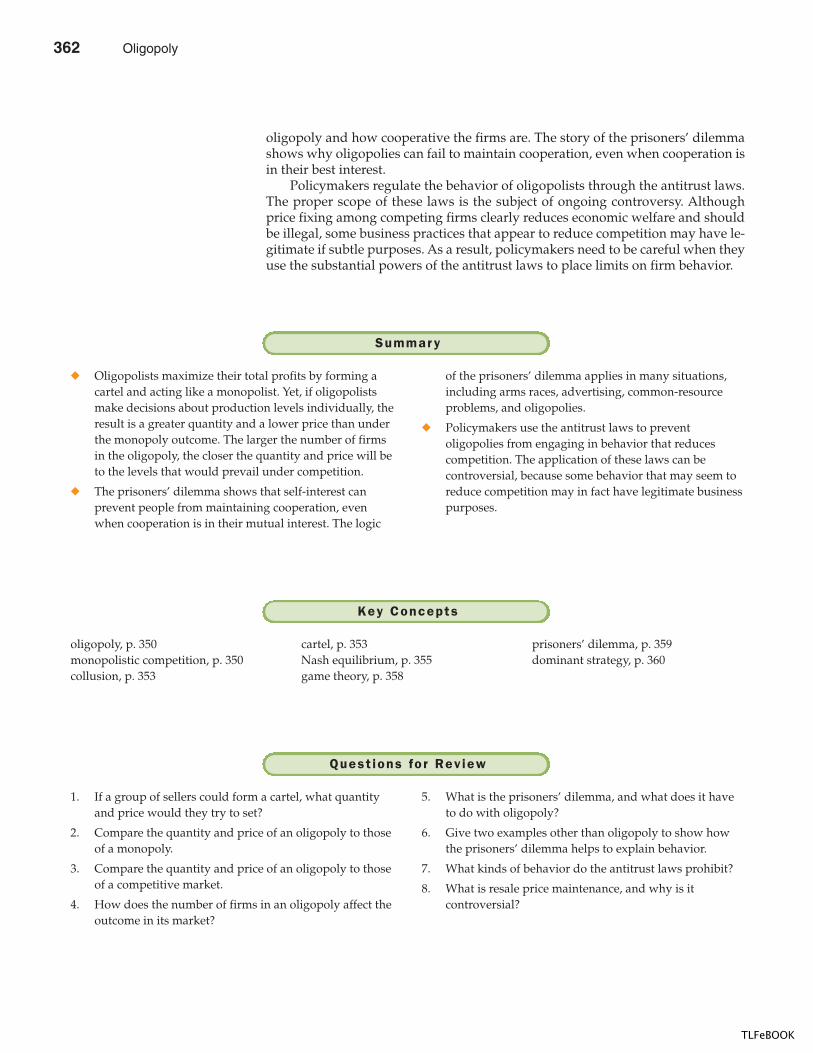
372 PART F IVE FIRM BEHAVIOR AND THE ORGANIZATION OF INDUSTRY
oligopoly and how cooperative the firms are. The story of the prisoners’ dilemmashows why oligopolies can fail to maintain cooperation, even when cooperation isin their best interest.
Policymakers regulate the behavior of oligopolists through the antitrust laws.The proper scope of these laws is the subject of ongoing controversy. Althoughprice fixing among competing firms clearly reduces economic welfare and shouldbe illegal, some business practices that appear to reduce competition may have le-gitimate if subtle purposes. As a result, policymakers need to be careful when theyuse the substantial powers of the antitrust laws to place limits on firm behavior.
� Oligopolists maximize their total profits by forming acartel and acting like a monopolist. Yet, if oligopolistsmake decisions about production levels individually, theresult is a greater quantity and a lower price than underthe monopoly outcome. The larger the number of firmsin the oligopoly, the closer the quantity and price will beto the levels that would prevail under competition.
� The prisoners’ dilemma shows that self-interest canprevent people from maintaining cooperation, evenwhen cooperation is in their mutual interest. The logic
of the prisoners’ dilemma applies in many situations,including arms races, advertising, common-resourceproblems, and oligopolies.
� Policymakers use the antitrust laws to preventoligopolies from engaging in behavior that reducescompetition. The application of these laws can becontroversial, because some behavior that may seem toreduce competition may in fact have legitimate businesspurposes.
Summar y
oligopoly, p. 350monopolistic competition, p. 350collusion, p. 353
cartel, p. 353Nash equilibrium, p. 355game theory, p. 358
prisoners’ dilemma, p. 359dominant strategy, p. 360
Key Concepts
1. If a group of sellers could form a cartel, what quantityand price would they try to set?
2. Compare the quantity and price of an oligopoly to thoseof a monopoly.
3. Compare the quantity and price of an oligopoly to thoseof a competitive market.
4. How does the number of firms in an oligopoly affect theoutcome in its market?
5. What is the prisoners’ dilemma, and what does it haveto do with oligopoly?
6. Give two examples other than oligopoly to show howthe prisoners’ dilemma helps to explain behavior.
7. What kinds of behavior do the antitrust laws prohibit?
8. What is resale price maintenance, and why is itcontroversial?
Quest ions fo r Rev iew
362 Oligopoly
TLFeBOOK
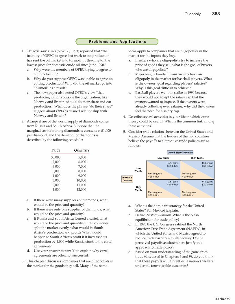
CHAPTER 16 OLIGOPOLY 373
1. The New York Times (Nov. 30, 1993) reported that “theinability of OPEC to agree last week to cut productionhas sent the oil market into turmoil . . . [leading to] thelowest price for domestic crude oil since June 1990.”a. Why were the members of OPEC trying to agree to
cut production?b. Why do you suppose OPEC was unable to agree on
cutting production? Why did the oil market go into“turmoil” as a result?
c. The newspaper also noted OPEC’s view “thatproducing nations outside the organization, likeNorway and Britain, should do their share and cutproduction.” What does the phrase “do their share”suggest about OPEC’s desired relationship withNorway and Britain?
2. A large share of the world supply of diamonds comesfrom Russia and South Africa. Suppose that themarginal cost of mining diamonds is constant at $1,000per diamond, and the demand for diamonds isdescribed by the following schedule:
PRICE QUANTITY
$8,000 5,0007,000 6,0006,000 7,0005,000 8,0004,000 9,0003,000 10,0002,000 11,0001,000 12,000
a. If there were many suppliers of diamonds, whatwould be the price and quantity?
b. If there were only one supplier of diamonds, whatwould be the price and quantity?
c. If Russia and South Africa formed a cartel, whatwould be the price and quantity? If the countriessplit the market evenly, what would be SouthAfrica’s production and profit? What wouldhappen to South Africa’s profit if it increased itsproduction by 1,000 while Russia stuck to the cartelagreement?
d. Use your answer to part (c) to explain why cartelagreements are often not successful.
3. This chapter discusses companies that are oligopolists inthe market for the goods they sell. Many of the same
ideas apply to companies that are oligopolists in themarket for the inputs they buy.a. If sellers who are oligopolists try to increase the
price of goods they sell, what is the goal of buyerswho are oligopolists?
b. Major league baseball team owners have anoligopoly in the market for baseball players. Whatis the owners’ goal regarding players’ salaries?Why is this goal difficult to achieve?
c. Baseball players went on strike in 1994 becausethey would not accept the salary cap that theowners wanted to impose. If the owners werealready colluding over salaries, why did the ownersfeel the need for a salary cap?
4. Describe several activities in your life in which gametheory could be useful. What is the common link amongthese activities?
5. Consider trade relations between the United States andMexico. Assume that the leaders of the two countriesbelieve the payoffs to alternative trade policies are asfollows:
a. What is the dominant strategy for the UnitedStates? For Mexico? Explain.
b. Define Nash equilibrium. What is the Nashequilibrium for trade policy?
c. In 1993 the U.S. Congress ratified the NorthAmerican Free Trade Agreement (NAFTA), inwhich the United States and Mexico agreed toreduce trade barriers simultaneously. Do theperceived payoffs as shown here justify thisapproach to trade policy?
d. Based on your understanding of the gains fromtrade (discussed in Chapters 3 and 9), do you thinkthat these payoffs actually reflect a nation’s welfareunder the four possible outcomes?
United States Decision
LowTariffs
Low Tariffs
U.S. gains$25 billion
Mexico gains$25 billion
Mexico gains$10 billion
Mexico gains$30 billion
Mexico gains$20 billion
U.S. gains$30 billion
U.S. gains$10 billion
U.S. gains$20 billion
High Tariffs
HighTarrifs
Mexico'sDecision
'
P rob lems and App l icat ions
Oligopoly 363
TLFeBOOK
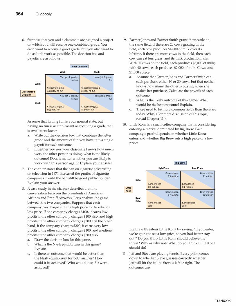
374 PART F IVE FIRM BEHAVIOR AND THE ORGANIZATION OF INDUSTRY
6. Suppose that you and a classmate are assigned a projecton which you will receive one combined grade. Youeach want to receive a good grade, but you also want todo as little work as possible. The decision box andpayoffs are as follows:
Assume that having fun is your normal state, buthaving no fun is as unpleasant as receiving a grade thatis two letters lower.a. Write out the decision box that combines the letter
grade and the amount of fun you have into a singlepayoff for each outcome.
b. If neither you nor your classmate knows how muchwork the other person is doing, what is the likelyoutcome? Does it matter whether you are likely towork with this person again? Explain your answer.
7. The chapter states that the ban on cigarette advertisingon television in 1971 increased the profits of cigarettecompanies. Could the ban still be good public policy?Explain your answer.
8. A case study in the chapter describes a phoneconversation between the presidents of AmericanAirlines and Braniff Airways. Let’s analyze the gamebetween the two companies. Suppose that eachcompany can charge either a high price for tickets or alow price. If one company charges $100, it earns lowprofits if the other company charges $100 also, and highprofits if the other company charges $200. On the otherhand, if the company charges $200, it earns very lowprofits if the other company charges $100, and mediumprofits if the other company charges $200 also.a. Draw the decision box for this game.b. What is the Nash equilibrium in this game?
Explain.c. Is there an outcome that would be better than
the Nash equilibrium for both airlines? Howcould it be achieved? Who would lose if it wereachieved?
9. Farmer Jones and Farmer Smith graze their cattle onthe same field. If there are 20 cows grazing in thefield, each cow produces $4,000 of milk over itslifetime. If there are more cows in the field, then eachcow can eat less grass, and its milk production falls.With 30 cows on the field, each produces $3,000 of milk;with 40 cows, each produces $2,000 of milk. Cows cost$1,000 apiece.a. Assume that Farmer Jones and Farmer Smith can
each purchase either 10 or 20 cows, but that neitherknows how many the other is buying when shemakes her purchase. Calculate the payoffs of eachoutcome.
b. What is the likely outcome of this game? Whatwould be the best outcome? Explain.
c. There used to be more common fields than there aretoday. Why? (For more discussion of this topic,reread Chapter 11.)
10. Little Kona is a small coffee company that is consideringentering a market dominated by Big Brew. Eachcompany’s profit depends on whether Little Konaenters and whether Big Brew sets a high price or a lowprice:
Big Brew threatens Little Kona by saying, “If you enter,we’re going to set a low price, so you had better stayout.” Do you think Little Kona should believe thethreat? Why or why not? What do you think Little Konashould do?
11. Jeff and Steve are playing tennis. Every point comesdown to whether Steve guesses correctly whetherJeff will hit the ball to Steve’s left or right. Theoutcomes are:
Big Brew
Enter
High Price
Brew makes$3 million
Kona makes$2 million
Kona loses$1 million
Kona makeszero
Kona makeszero
Brew makes$1 million
Brew makes$7 million
Brew makes$2 million
Low Price
Don'tEnter
LittleKona
Your Decision
Work
Work
You get A grade,no fun
Classmate gets A grade, no fun
Classmate gets B grade, no fun
Classmate gets B grade, fun
Classmate gets D grade, fun
You get B grade,fun
You get B grade,no fun
You get D grade,fun
Shirk
Shirk
Classmate'sDecision
364 Oligopoly
TLFeBOOK
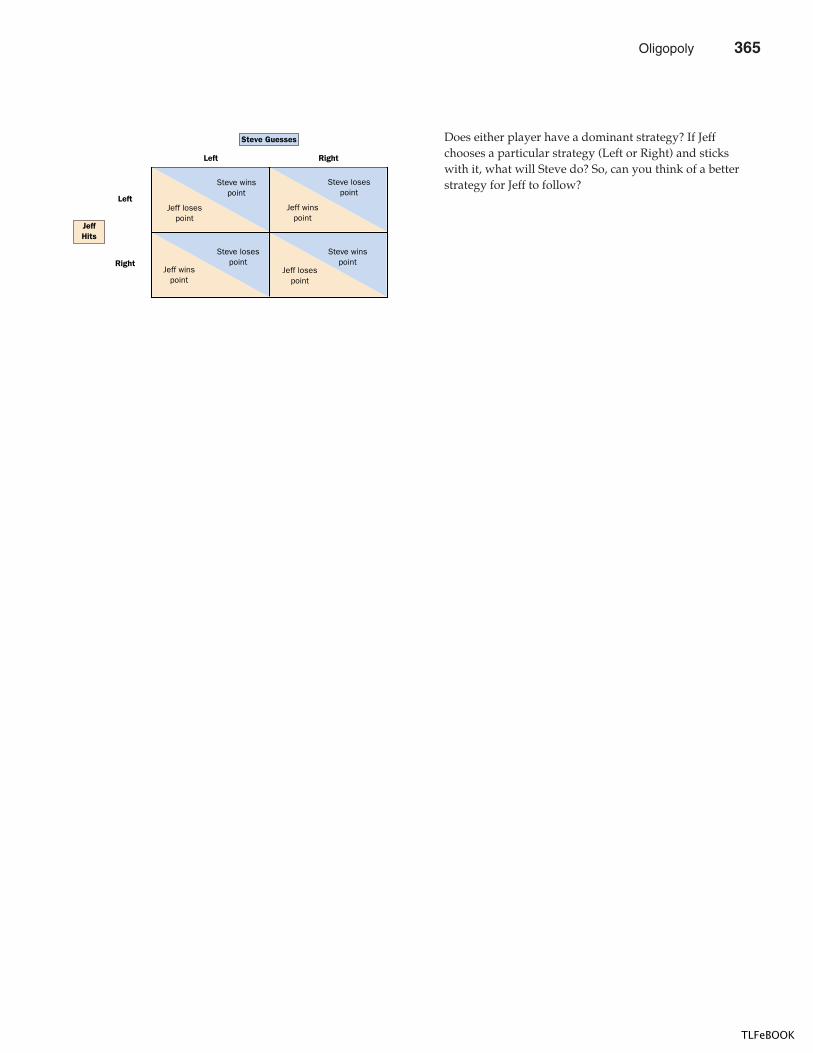
CHAPTER 16 OLIGOPOLY 375
Does either player have a dominant strategy? If Jeffchooses a particular strategy (Left or Right) and stickswith it, what will Steve do? So, can you think of a betterstrategy for Jeff to follow?
Steve Guesses
Left
Left
Steve winspoint
Jeff winspoint
Jeff winspoint
Steve winspoint
Right
Right
JeffHits
Jeff losespoint
Steve losespoint
Steve losespoint
Jeff losespoint
Oligopoly 365
TLFeBOOK

TLFeBOOK
IN THIS CHAPTERYOU WILL . . .
Examine the debateover the ro le o f
brand names
Cons ider thedes i rab i l i ty o foutcomes in
monopol is t ica l l ycompet i t i ve
markets
Analyze compet i t ionamong f i rms that
se l l d i f fe rent iatedproducts
Compare theoutcome undermonopol is t ic
compet i t ion andunder per fectcompet i t ion
Examine the debateover the e f fects o f
adver t is ing
You walk into a bookstore to buy a book to read during your next vacation. On thestore’s shelves you find a John Grisham mystery, a Stephen King thriller, a DanielleSteel romance, a Frank McCourt memoir, and many other choices. When you pickout a book and buy it, what kind of market are you participating in?
On the one hand, the market for books seems competitive. As you look overthe shelves at your bookstore, you find many authors and many publishers vyingfor your attention. A buyer in this market has thousands of competing productsfrom which to choose. And because anyone can enter the industry by writing andpublishing a book, the book business is not very profitable. For every highly paidnovelist, there are hundreds of struggling ones.
On the other hand, the market for books seems monopolistic. Because eachbook is unique, publishers have some latitude in choosing what price to charge.The sellers in this market are price makers rather than price takers. And, indeed,the price of books greatly exceeds marginal cost. The price of a typical hardcover
M O N O P O L I S T I C C O M P E T I T I O N
377
367
17
TLFeBOOK
378 PART F IVE FIRM BEHAVIOR AND THE ORGANIZATION OF INDUSTRY
novel, for instance, is about $25, whereas the cost of printing one additional copyof the novel is less than $5.
In this chapter we examine markets that have some features of competi-tion and some features of monopoly. This market structure is called monopolisticcompetition. Monopolistic competition describes a market with the followingattributes:
� Many sellers: There are many firms competing for the same group ofcustomers.
� Product differentiation: Each firm produces a product that is at least slightlydifferent from those of other firms. Thus, rather than being a price taker, eachfirm faces a downward-sloping demand curve.
� Free entry: Firms can enter (or exit) the market without restriction. Thus,the number of firms in the market adjusts until economic profits are drivento zero.
A moment’s thought reveals a long list of markets with these attributes: books,CDs, movies, computer games, restaurants, piano lessons, cookies, furniture, andso on.
Monopolistic competition, like oligopoly, is a market structure that lies be-tween the extreme cases of competition and monopoly. But oligopoly and monop-olistic competition are quite different. Oligopoly departs from the perfectlycompetitive ideal of Chapter 14 because there are only a few sellers in the market.The small number of sellers makes rigorous competition less likely, and it makesstrategic interactions among them vitally important. By contrast, under monopo-listic competition, there are many sellers, each of which is small compared to themarket. A monopolistically competitive market departs from the perfectly com-petitive ideal because each of the sellers offers a somewhat different product.
COMPETIT ION WITH DIFFERENTIATED PRODUCTS
To understand monopolistically competitive markets, we first consider the de-cisions facing an individual firm. We then examine what happens in the longrun as firms enter and exit the industry. Next, we compare the equilibrium un-der monopolistic competition to the equilibrium under perfect competition thatwe examined in Chapter 14. Finally, we consider whether the outcome in a mo-nopolistically competitive market is desirable from the standpoint of society as awhole.
THE MONOPOLISTICALLY COMPETIT IVEFIRM IN THE SHORT RUN
Each firm in a monopolistically competitive market is, in many ways, like a mo-nopoly. Because its product is different from those offered by other firms, it faces a
monopol is t ic compet i t iona market structure in which manyfirms sell products that are similarbut not identical
368 Monopolistic Competition
TLFeBOOK
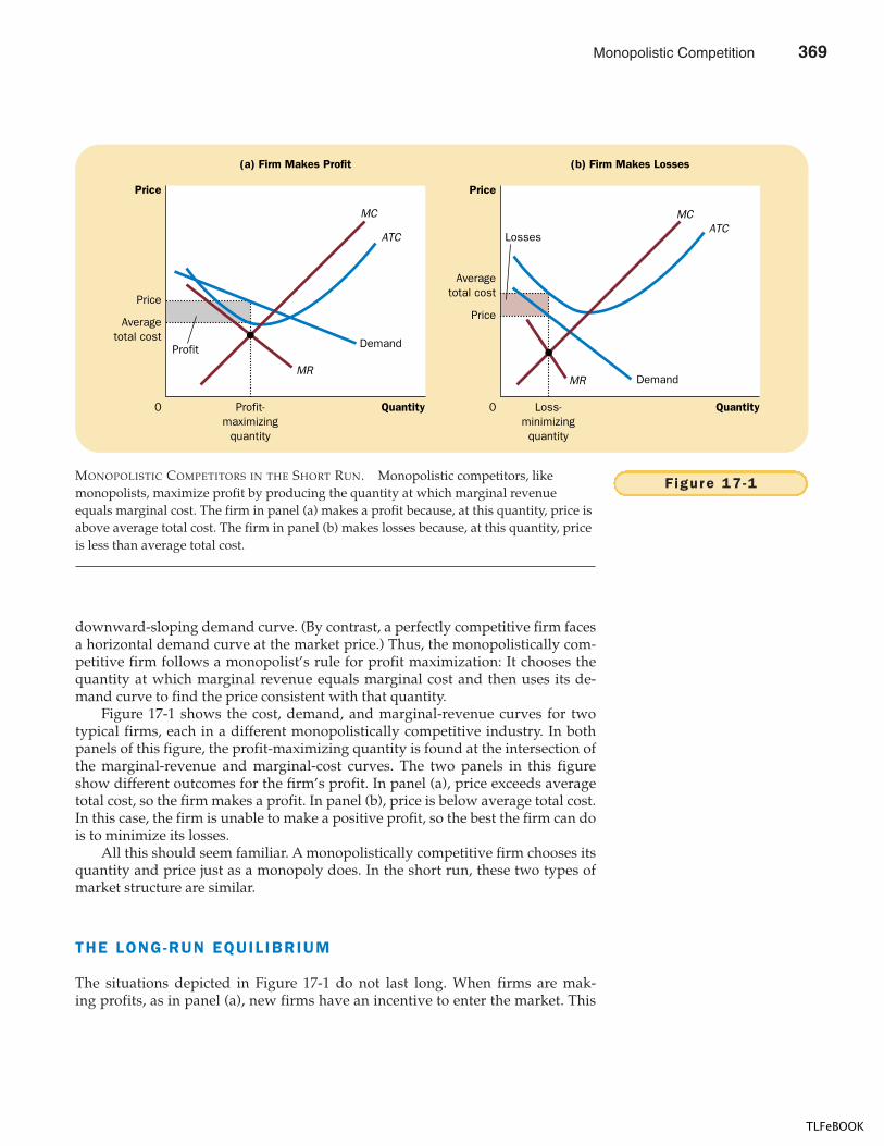
CHAPTER 17 MONOPOLISTIC COMPETIT ION 379
downward-sloping demand curve. (By contrast, a perfectly competitive firm facesa horizontal demand curve at the market price.) Thus, the monopolistically com-petitive firm follows a monopolist’s rule for profit maximization: It chooses thequantity at which marginal revenue equals marginal cost and then uses its de-mand curve to find the price consistent with that quantity.
Figure 17-1 shows the cost, demand, and marginal-revenue curves for twotypical firms, each in a different monopolistically competitive industry. In bothpanels of this figure, the profit-maximizing quantity is found at the intersection ofthe marginal-revenue and marginal-cost curves. The two panels in this figureshow different outcomes for the firm’s profit. In panel (a), price exceeds averagetotal cost, so the firm makes a profit. In panel (b), price is below average total cost.In this case, the firm is unable to make a positive profit, so the best the firm can dois to minimize its losses.
All this should seem familiar. A monopolistically competitive firm chooses itsquantity and price just as a monopoly does. In the short run, these two types ofmarket structure are similar.
THE LONG-RUN EQUIL IBRIUM
The situations depicted in Figure 17-1 do not last long. When firms are mak-ing profits, as in panel (a), new firms have an incentive to enter the market. This
QuantityProfit-maximizing
quantity
Loss-minimizingquantity
0
Price
Price
Demand
DemandMR
ATC
(a) Firm Makes Profit
Quantity0
Price
PriceAverage
total cost
Averagetotal cost
(b) Firm Makes Losses
MR
Profit
Losses
MCATC
MC
Figure 17 -1MONOPOLISTIC COMPETITORS IN THE SHORT RUN. Monopolistic competitors, likemonopolists, maximize profit by producing the quantity at which marginal revenueequals marginal cost. The firm in panel (a) makes a profit because, at this quantity, price isabove average total cost. The firm in panel (b) makes losses because, at this quantity, priceis less than average total cost.
Monopolistic Competition 369
TLFeBOOK
380 PART F IVE FIRM BEHAVIOR AND THE ORGANIZATION OF INDUSTRY
entry increases the number of products from which customers can choose and,therefore, reduces the demand faced by each firm already in the market. In otherwords, profit encourages entry, and entry shifts the demand curves faced by theincumbent firms to the left. As the demand for incumbent firms’ products falls,these firms experience declining profit.
Conversely, when firms are making losses, as in panel (b), firms in the markethave an incentive to exit. As firms exit, customers have fewer products from whichto choose. This decrease in the number of firms expands the demand faced bythose firms that stay in the market. In other words, losses encourage exit, and exitshifts the demand curves of the remaining firms to the right. As the demand forthe remaining firms’ products rises, these firms experience rising profit (that is, de-clining losses).
This process of entry and exit continues until the firms in the market are mak-ing exactly zero economic profit. Figure 17-2 depicts the long-run equilibrium.Once the market reaches this equilibrium, new firms have no incentive to enter,and existing firms have no incentive to exit.
Notice that the demand curve in this figure just barely touches the average-total-cost curve. Mathematically, we say the two curves are tangent to each other.These two curves must be tangent once entry and exit have driven profit to zero.Because profit per unit sold is the difference between price (found on the demandcurve) and average total cost, the maximum profit is zero only if these two curvestouch each other without crossing.
370 Monopolistic Competition
TLFeBOOK
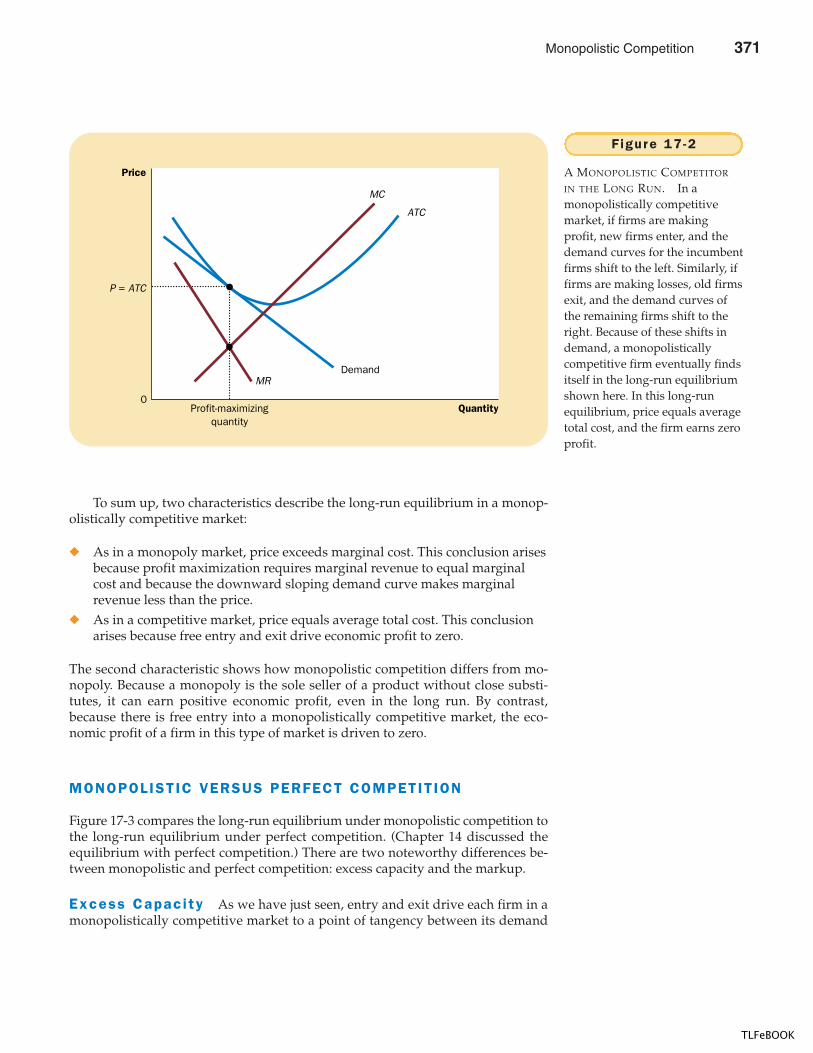
CHAPTER 17 MONOPOLISTIC COMPETIT ION 381
To sum up, two characteristics describe the long-run equilibrium in a monop-olistically competitive market:
� As in a monopoly market, price exceeds marginal cost. This conclusion arisesbecause profit maximization requires marginal revenue to equal marginalcost and because the downward sloping demand curve makes marginalrevenue less than the price.
� As in a competitive market, price equals average total cost. This conclusionarises because free entry and exit drive economic profit to zero.
The second characteristic shows how monopolistic competition differs from mo-nopoly. Because a monopoly is the sole seller of a product without close substi-tutes, it can earn positive economic profit, even in the long run. By contrast,because there is free entry into a monopolistically competitive market, the eco-nomic profit of a firm in this type of market is driven to zero.
MONOPOLISTIC VERSUS PERFECT COMPETIT ION
Figure 17-3 compares the long-run equilibrium under monopolistic competition tothe long-run equilibrium under perfect competition. (Chapter 14 discussed theequilibrium with perfect competition.) There are two noteworthy differences be-tween monopolistic and perfect competition: excess capacity and the markup.
Excess Capaci ty As we have just seen, entry and exit drive each firm in amonopolistically competitive market to a point of tangency between its demand
Profit-maximizingquantity
Quantity
Price
0
P = ATC
DemandMR
ATC
MC
Figure 17 -2
A MONOPOLISTIC COMPETITOR
IN THE LONG RUN. In amonopolistically competitivemarket, if firms are makingprofit, new firms enter, and thedemand curves for the incumbentfirms shift to the left. Similarly, iffirms are making losses, old firmsexit, and the demand curves ofthe remaining firms shift to theright. Because of these shifts indemand, a monopolisticallycompetitive firm eventually findsitself in the long-run equilibriumshown here. In this long-runequilibrium, price equals averagetotal cost, and the firm earns zeroprofit.
Monopolistic Competition 371
TLFeBOOK
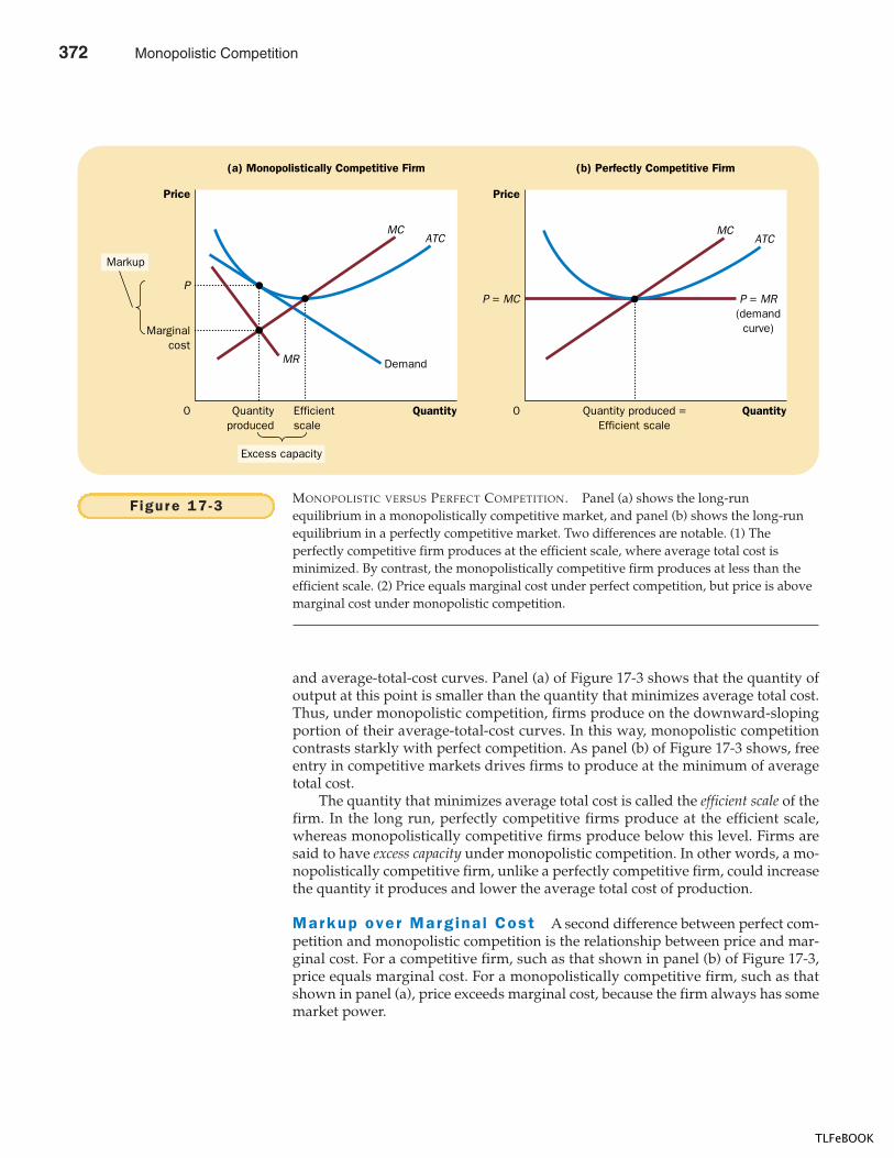
382 PART F IVE FIRM BEHAVIOR AND THE ORGANIZATION OF INDUSTRY
and average-total-cost curves. Panel (a) of Figure 17-3 shows that the quantity ofoutput at this point is smaller than the quantity that minimizes average total cost.Thus, under monopolistic competition, firms produce on the downward-slopingportion of their average-total-cost curves. In this way, monopolistic competitioncontrasts starkly with perfect competition. As panel (b) of Figure 17-3 shows, freeentry in competitive markets drives firms to produce at the minimum of averagetotal cost.
The quantity that minimizes average total cost is called the efficient scale of thefirm. In the long run, perfectly competitive firms produce at the efficient scale,whereas monopolistically competitive firms produce below this level. Firms aresaid to have excess capacity under monopolistic competition. In other words, a mo-nopolistically competitive firm, unlike a perfectly competitive firm, could increasethe quantity it produces and lower the average total cost of production.
Markup over Marg ina l Cost A second difference between perfect com-petition and monopolistic competition is the relationship between price and mar-ginal cost. For a competitive firm, such as that shown in panel (b) of Figure 17-3,price equals marginal cost. For a monopolistically competitive firm, such as thatshown in panel (a), price exceeds marginal cost, because the firm always has somemarket power.
QuantityQuantityproduced
Efficientscale
Quantity produced =Efficient scale
0
Price
P
Demand
(a) Monopolistically Competitive Firm
Quantity0
Price
P = MC P = MR(demandcurve)Marginal
cost
(b) Perfectly Competitive Firm
Markup
Excess capacity
MCATC
MCATC
MR
Figure 17 -3 MONOPOLISTIC VERSUS PERFECT COMPETITION. Panel (a) shows the long-runequilibrium in a monopolistically competitive market, and panel (b) shows the long-runequilibrium in a perfectly competitive market. Two differences are notable. (1) Theperfectly competitive firm produces at the efficient scale, where average total cost isminimized. By contrast, the monopolistically competitive firm produces at less than theefficient scale. (2) Price equals marginal cost under perfect competition, but price is abovemarginal cost under monopolistic competition.
372 Monopolistic Competition
TLFeBOOK
CHAPTER 17 MONOPOLISTIC COMPETIT ION 383
How is this markup over marginal cost consistent with free entry and zeroprofit? The zero-profit condition ensures only that price equals average totalcost. It does not ensure that price equals marginal cost. Indeed, in the long-runequilibrium, monopolistically competitive firms operate on the declining por-tion of their average-total-cost curves, so marginal cost is below average to-tal cost. Thus, for price to equal average total cost, price must be above marginalcost.
In this relationship between price and marginal cost, we see a key behavioraldifference between perfect competitors and monopolistic competitors. Imaginethat you were to ask a firm the following question: “Would you like to see anothercustomer come through your door ready to buy from you at your current price?”A perfectly competitive firm would answer that it didn’t care. Because price ex-actly equals marginal cost, the profit from an extra unit sold is zero. By contrast, amonopolistically competitive firm is always eager to get another customer. Be-cause its price exceeds marginal cost, an extra unit sold at the posted price meansmore profit. According to an old quip, monopolistically competitive markets arethose in which sellers send Christmas cards to the buyers.
MONOPOLISTIC COMPETIT ION ANDTHE WELFARE OF SOCIETY
Is the outcome in a monopolistically competitive market desirable from the stand-point of society as a whole? Can policymakers improve on the market outcome?There are no simple answers to these questions.
One source of inefficiency is the markup of price over marginal cost. Becauseof the markup, some consumers who value the good at more than the marginalcost of production (but less than the price) will be deterred from buying it. Thus, amonopolistically competitive market has the normal deadweight loss of monopolypricing. We first saw this type of inefficiency when we discussed monopoly inChapter 15.
Although this outcome is clearly undesirable compared to the first-best out-come of price equal to marginal cost, there is no easy way for policymakers to fixthe problem. To enforce marginal-cost pricing, policymakers would need to regu-late all firms that produce differentiated products. Because such products are socommon in the economy, the administrative burden of such regulation would beoverwhelming.
Moreover, regulating monopolistic competitors would entail all the problemsof regulating natural monopolies. In particular, because monopolistic competitorsare making zero profits already, requiring them to lower their prices to equal mar-ginal cost would cause them to make losses. To keep these firms in business, thegovernment would need to help them cover these losses. Rather than raising taxesto pay for these subsidies, policymakers may decide it is better to live with theinefficiency of monopolistic pricing.
Another way in which monopolistic competition may be socially inefficient isthat the number of firms in the market may not be the “ideal” one. That is, theremay be too much or too little entry. One way to think about this problem is interms of the externalities associated with entry. Whenever a new firm considers en-tering the market with a new product, it considers only the profit it would make.Yet its entry would also have two external effects:
Monopolistic Competition 373
TLFeBOOK
384 PART F IVE FIRM BEHAVIOR AND THE ORGANIZATION OF INDUSTRY
� The product-variety externality: Because consumers get some consumer surplusfrom the introduction of a new product, entry of a new firm conveys apositive externality on consumers.
� The business-stealing externality: Because other firms lose customers andprofits from the entry of a new competitor, entry of a new firm imposes anegative externality on existing firms.
Thus, in a monopolistically competitive market, there are both positive and nega-tive externalities associated with the entry of new firms. Depending on which ex-ternality is larger, a monopolistically competitive market could have either too fewor too many products.
Both of these externalities are closely related to the conditions for monopolis-tic competition. The product-variety externality arises because a new firm wouldoffer a product different from those of the existing firms. The business-stealing ex-ternality arises because firms post a price above marginal cost and, therefore, arealways eager to sell additional units. Conversely, because perfectly competitivefirms produce identical goods and charge a price equal to marginal cost, neither ofthese externalities exists under perfect competition.
In the end, we can conclude only that monopolistically competitive marketsdo not have all the desirable welfare properties of perfectly competitive markets.That is, the invisible hand does not ensure that total surplus is maximized undermonopolistic competition. Yet because the inefficiencies are subtle, hard to mea-sure, and hard to fix, there is no easy way for public policy to improve the marketoutcome.
QUICK QUIZ: List the three key attributes of monopolistic competition.� Draw and explain a diagram to show the long-run equilibrium in a monopolistically competitive market. How does this equilibrium differ from that in a perfectly competitive market?
As we have seen, monopolisti-cally competitive firms producea quantity of output below thelevel that minimizes average to-tal cost. By contrast, firms inperfectly competitive marketsare driven to produce at thequantity that minimizes averagetotal cost. This comparison be-tween perfect and monopolisticcompetition has led someeconomists in the past to ar-gue that the excess capacity of
monopolistic competitors was a source of inefficiency.Today economists understand that the excess capac-
ity of monopolistic competitors is not directly relevant for
evaluating economic welfare. There is no reason that soci-ety should want all firms to produce at the minimum ofaverage total cost. For example, consider a publishing firm.Producing a novel might take a fixed cost of $50,000 (theauthor’s time) and variable costs of $5 per book (the cost ofprinting). In this case, the average total cost of a book de-clines as the number of books increases because the fixedcost gets spread over more and more units. The average to-tal cost is minimized by printing an infinite number of books.But in no sense is infinity the right number of books for so-ciety to produce.
In short, monopolistic competitors do have excess ca-pacity, but this fact tells us little about the desirability of themarket outcome.
FYI
Is ExcessCapacity a
Social Problem?
374 Monopolistic Competition
TLFeBOOK
CHAPTER 17 MONOPOLISTIC COMPETIT ION 385
ADVERTISING
It is nearly impossible to go through a typical day in a modern economy withoutbeing bombarded with advertising. Whether you are reading a newspaper, watch-ing television, or driving down the highway, some firm will try to convince you tobuy its product. Such behavior is a natural feature of monopolistic competition.When firms sell differentiated products and charge prices above marginal cost,each firm has an incentive to advertise in order to attract more buyers to its partic-ular product.
The amount of advertising varies substantially across products. Firms that sellhighly differentiated consumer goods, such as over-the-counter drugs, perfumes,soft drinks, razor blades, breakfast cereals, and dog food, typically spend between10 and 20 percent of revenue for advertising. Firms that sell industrial products,such as drill presses and communications satellites, typically spend very little onadvertising. And firms that sell homogeneous products, such as wheat, peanuts, orcrude oil, spend nothing at all. For the economy as a whole, spending on advertis-ing comprises about 2 percent of total firm revenue, or more than $100 billion.
Advertising takes many forms. About one-half of advertising spending is forspace in newspapers and magazines, and about one-third is for commercials ontelevision and radio. The rest is spent on various other ways of reaching cus-tomers, such as direct mail, billboards, and the Goodyear blimp.
THE DEBATE OVER ADVERTISING
Is society wasting the resources it devotes to advertising? Or does advertisingserve a valuable purpose? Assessing the social value of advertising is difficult andoften generates heated argument among economists. Let’s consider both sides ofthe debate.
The Cr i t ique o f Adver t is ing Critics of advertising argue that firms ad-vertise in order to manipulate people’s tastes. Much advertising is psychologicalrather than informational. Consider, for example, the typical television commercialfor some brand of soft drink. The commercial most likely does not tell the viewerabout the product’s price or quality. Instead, it might show a group of happy peo-ple at a party on a beach on a beautiful sunny day. In their hands are cans of thesoft drink. The goal of the commercial is to convey a subconscious (if not subtle)message: “You too can have many friends and be happy, if only you drink ourproduct.” Critics of advertising argue that such a commercial creates a desire thatotherwise might not exist.
Critics also argue that advertising impedes competition. Advertising oftentries to convince consumers that products are more different than they truly are.By increasing the perception of product differentiation and fostering brand loyalty,advertising makes buyers less concerned with price differences among similargoods. With a less elastic demand curve, each firm charges a larger markup overmarginal cost.
The Defense o f Adver t is ing Defenders of advertising argue that firmsuse advertising to provide information to customers. Advertising conveys the
Monopolistic Competition 375
TLFeBOOK
386 PART F IVE FIRM BEHAVIOR AND THE ORGANIZATION OF INDUSTRY
CASE STUDY ADVERTISING AND THE PRICE OF EYEGLASSES
What effect does advertising have on the price of a good? On the one hand, ad-vertising might make consumers view products as being more different thanthey otherwise would. If so, it would make markets less competitive and firms’demand curves less elastic, and this would lead firms to charge higher prices.On the other hand, advertising might make it easier for consumers to find thefirms offering the best prices. In this case, it would make markets more com-petitive and firms’ demand curves more elastic, and this would lead to lowerprices.
In an article published in the Journal of Law and Economics in 1972, economistLee Benham tested these two views of advertising. In the United States duringthe 1960s, the various state governments had vastly different rules about adver-tising by optometrists. Some states allowed advertising for eyeglasses and eyeexaminations. Many states, however, prohibited it. For example, the Florida lawread as follows:
It is unlawful for any person, firm, or corporation to . . . advertise eitherdirectly or indirectly by any means whatsoever any definite or indefinite priceor credit terms on prescriptive or corrective lens, frames, completeprescriptive or corrective glasses, or any optometric service. . . . This section ispassed in the interest of public health, safety, and welfare, and its provisionsshall be liberally construed to carry out its objects and purposes.
Professional optometrists enthusiastically endorsed these restrictions onadvertising.
Benham used the differences in state law as a natural experiment to testthe two views of advertising. The results were striking. In those states that pro-hibited advertising, the average price paid for a pair of eyeglasses was $33.(This number is not as low as it seems, for this price is from 1963, when allprices were much lower than they are today. To convert 1963 prices into to-day’s dollars, you can multiply them by 5.) In those states that did not restrict
prices of the goods being offered for sale, the existence of new products, and thelocations of retail outlets. This information allows customers to make betterchoices about what to buy and, thus, enhances the ability of markets to allocate re-sources efficiently.
Defenders also argue that advertising fosters competition. Because advertisingallows customers to be more fully informed about all the firms in the market, cus-tomers can more easily take advantage of price differences. Thus, each firm hasless market power. In addition, advertising allows new firms to enter more easily,because it gives entrants a means to attract customers from existing firms.
Over time, policymakers have come to accept the view that advertising canmake markets more competitive. One important example is the regulation of cer-tain professions, such as lawyers, doctors, and pharmacists. In the past, thesegroups succeeded in getting state governments to prohibit advertising in theirfields on the grounds that advertising was “unprofessional.” In recent years, how-ever, the courts have concluded that the primary effect of these restrictions on ad-vertising was to curtail competition. They have, therefore, overturned many of thelaws that prohibit advertising by members of these professions.
376 Monopolistic Competition
TLFeBOOK
CHAPTER 17 MONOPOLISTIC COMPETIT ION 387
advertising, the average price was $26. Thus, advertising reduced averageprices by more than 20 percent. In the market for eyeglasses, and probably inmany other markets as well, advertising fosters competition and leads to lowerprices for consumers.
ADVERTISING AS A SIGNAL OF QUALITY
Many types of advertising contain little apparent information about the productbeing advertised. Consider a firm introducing a new breakfast cereal. A typical ad-vertisement might have some highly paid actor eating the cereal and exclaiminghow wonderful it tastes. How much information does the advertisement reallyprovide?
The answer is: more than you might think. Defenders of advertising argue thateven advertising that appears to contain little hard information may in fact tellconsumers something about product quality. The willingness of the firm to spenda large amount of money on advertising can itself be a signal to consumers aboutthe quality of the product being offered.
Consider the problem facing two firms—Post and Kellogg. Each company hasjust come up with a recipe for a new cereal, which it would sell for $3 a box. Tokeep things simple, let’s assume that the marginal cost of making cereal is zero, sothe $3 is all profit. Each company knows that if it spends $10 million on advertis-ing, it will get 1 million consumers to try its new cereal. And each company knowsthat if consumers like the cereal, they will buy it not once but many times.
First consider Post’s decision. Based on market research, Post knows that itscereal is only mediocre. Although advertising would sell one box to each of 1 mil-lion consumers, the consumers would quickly learn that the cereal is not verygood and stop buying it. Post decides it is not worth paying $10 million in adver-tising to get only $3 million in sales. So it does not bother to advertise. It sends itscooks back to the drawing board to find another recipe.
Kellogg, on the other hand, knows that its cereal is great. Each person whotries it will buy a box a month for the next year. Thus, the $10 million in advertis-ing will bring in $36 million in sales. Advertising is profitable here because Kellogghas a good product that consumers will buy repeatedly. Thus, Kellogg chooses toadvertise.
Now that we have considered the behavior of the two firms, let’s consider thebehavior of consumers. We began by asserting that consumers are inclined to try anew cereal that they see advertised. But is this behavior rational? Should a con-sumer try a new cereal just because the seller has chosen to advertise it?
In fact, it may be completely rational for consumers to try new products thatthey see advertised. In our story, consumers decide to try Kellogg’s new cereal be-cause Kellogg advertises. Kellogg chooses to advertise because it knows that its ce-real is quite good, while Post chooses not to advertise because it knows that itscereal is only mediocre. By its willingness to spend money on advertising, Kelloggsignals to consumers the quality of its cereal. Each consumer thinks, quite sensibly,“Boy, if the Kellogg Company is willing to spend so much money advertising thisnew cereal, it must be really good.”
What is most surprising about this theory of advertising is that the content ofthe advertisement is irrelevant. Kellogg signals the quality of its product by itswillingness to spend money on advertising. What the advertisements say is not as
Monopolistic Competition 377
TLFeBOOK
388 PART F IVE FIRM BEHAVIOR AND THE ORGANIZATION OF INDUSTRY
important as the fact that consumers know ads are expensive. By contrast, cheapadvertising cannot be effective at signaling quality to consumers. In our example,if an advertising campaign cost less than $3 million, both Post and Kellogg woulduse it to market their new cereals. Because both good and mediocre cereals wouldbe advertised, consumers could not infer the quality of a new cereal from thefact that it is advertised. Over time, consumers would learn to ignore such cheapadvertising.
This theory can explain why firms pay famous actors large amounts of moneyto make advertisements that, on the surface, appear to convey no information atall. The information is not in the advertisement’s content, but simply in its exis-tence and expense.
BRAND NAMES
Advertising is closely related to the existence of brand names. In many markets,there are two types of firms. Some firms sell products with widely recognizedbrand names, while other firms sell generic substitutes. For example, in a typicaldrugstore, you can find Bayer aspirin on the shelf next to a generic aspirin. In atypical grocery store, you can find Pepsi next to less familiar colas. Most often, thefirm with the brand name spends more on advertising and charges a higher pricefor its product.
Just as there is disagreement about the economics of advertising, there is dis-agreement about the economics of brand names. Let’s consider both sides of thedebate.
Critics of brand names argue that brand names cause consumers to perceivedifferences that do not really exist. In many cases, the generic good is almost in-distinguishable from the brand-name good. Consumers’ willingness to pay morefor the brand-name good, these critics assert, is a form of irrationality fostered byadvertising. Economist Edward Chamberlin, one of the early developers of thetheory of monopolistic competition, concluded from this argument that brandnames were bad for the economy. He proposed that the government discourage
378 Monopolistic Competition
TLFeBOOK
CHAPTER 17 MONOPOLISTIC COMPETIT ION 389
CASE STUDY BRAND NAMES UNDER COMMUNISM
Defenders of brand names get some support for their view from experiences inthe former Soviet Union. When the Soviet Union adhered to the principles ofcommunism, central planners in the government replaced the invisible hand ofthe marketplace. Yet, just like consumers living in an economy with free mar-kets, Soviet central planners learned that brand names were useful in helping toensure product quality.
In an article published in the Journal of Political Economy in 1960, MarshallGoldman, an expert on the Soviet economy, described the Soviet experience:
In the Soviet Union, production goals have been set almost solely inquantitative or value terms, with the result that, in order to meet the plan,quality is often sacrificed. . . . Among the methods adopted by the Soviets todeal with this problem, one is of particular interest to us—intentional productdifferentiation. . . . In order to distinguish one firm from similar firms in thesame industry or ministry, each firm has its own name. Whenever it is
their use by refusing to enforce the exclusive trademarks that companies use toidentify their products.
More recently, economists have defended brand names as a useful way forconsumers to ensure that the goods they buy are of high quality. There are two re-lated arguments. First, brand names provide consumers information about qualitywhen quality cannot be easily judged in advance of purchase. Second, brandnames give firms an incentive to maintain high quality, because firms have a finan-cial stake in maintaining the reputation of their brand names.
To see how these arguments work in practice, consider a famous brand name:McDonald’s hamburgers. Imagine that you are driving through an unfamiliartown and want to stop for lunch. You see a McDonald’s and a local restaurant nextto it. Which do you choose? The local restaurant may in fact offer better food atlower prices, but you have no way of knowing that. By contrast, McDonald’s of-fers a consistent product across many cities. Its brand name is useful to you as away of judging the quality of what you are about to buy.
The McDonald’s brand name also ensures that the company has an incentiveto maintain quality. For example, if some customers were to become ill from badfood sold at a McDonald’s, the news would be disastrous for the company.McDonald’s would lose much of the valuable reputation that it has built up withyears of expensive advertising. As a result, it would lose sales and profit not just inthe outlet that sold the bad food but in its many outlets throughout the country.By contrast, if some customers were to become ill from bad food at a local restau-rant, that restaurant might have to close down, but the lost profits would bemuch smaller. Hence, McDonald’s has a greater incentive to ensure that its foodis safe.
The debate over brand names thus centers on the question of whether con-sumers are rational in preferring brand names over generic substitutes. Critics ofbrand names argue that brand names are the result of an irrational consumer re-sponse to advertising. Defenders of brand names argue that consumers have goodreason to pay more for brand-name products because they can be more confidentin the quality of these products.
Monopolistic Competition 379
TLFeBOOK
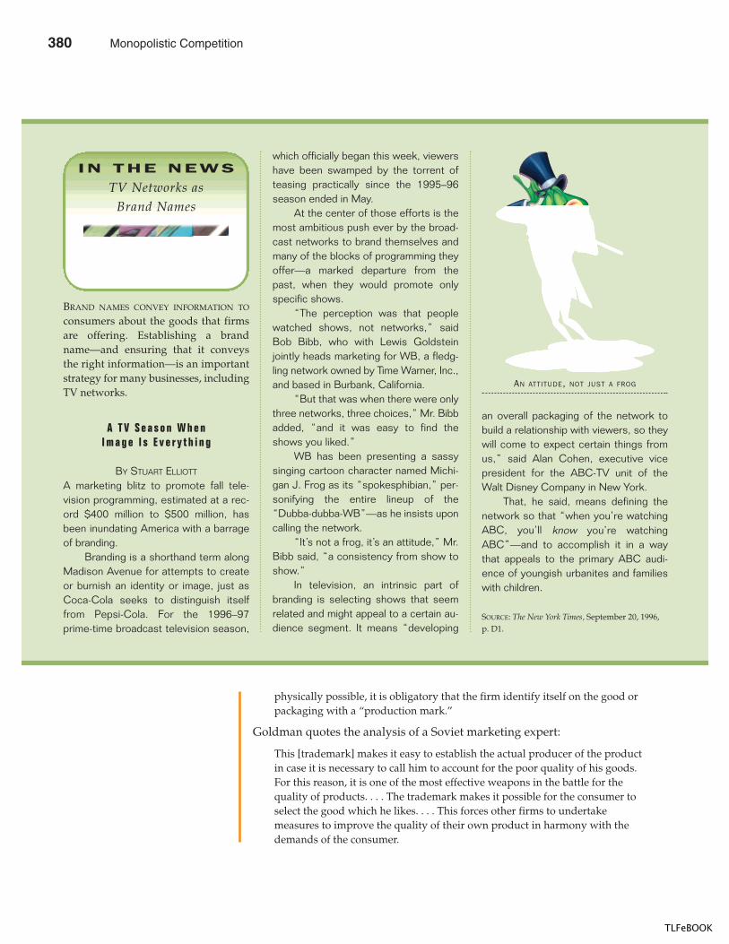
390 PART F IVE FIRM BEHAVIOR AND THE ORGANIZATION OF INDUSTRY
physically possible, it is obligatory that the firm identify itself on the good orpackaging with a “production mark.”
Goldman quotes the analysis of a Soviet marketing expert:
This [trademark] makes it easy to establish the actual producer of the productin case it is necessary to call him to account for the poor quality of his goods.For this reason, it is one of the most effective weapons in the battle for thequality of products. . . . The trademark makes it possible for the consumer toselect the good which he likes. . . . This forces other firms to undertakemeasures to improve the quality of their own product in harmony with thedemands of the consumer.
BRAND NAMES CONVEY INFORMATION TO
consumers about the goods that firmsare offering. Establishing a brandname—and ensuring that it conveysthe right information—is an importantstrategy for many businesses, includingTV networks.
A T V S e a s o n W h e nI m a g e I s E v e r y t h i n g
BY STUART ELLIOTT
A marketing blitz to promote fall tele-vision programming, estimated at a rec-ord $400 million to $500 million, hasbeen inundating America with a barrageof branding.
Branding is a shorthand term alongMadison Avenue for attempts to createor burnish an identity or image, just asCoca-Cola seeks to distinguish itselffrom Pepsi-Cola. For the 1996–97prime-time broadcast television season,
which officially began this week, viewershave been swamped by the torrent ofteasing practically since the 1995–96season ended in May.
At the center of those efforts is themost ambitious push ever by the broad-cast networks to brand themselves andmany of the blocks of programming theyoffer—a marked departure from thepast, when they would promote onlyspecific shows.
“The perception was that peoplewatched shows, not networks,” saidBob Bibb, who with Lewis Goldsteinjointly heads marketing for WB, a fledg-ling network owned by Time Warner, Inc.,and based in Burbank, California.
“But that was when there were onlythree networks, three choices,” Mr. Bibbadded, “and it was easy to find theshows you liked.”
WB has been presenting a sassysinging cartoon character named Michi-gan J. Frog as its “spokesphibian,” per-sonifying the entire lineup of the“Dubba-dubba-WB”—as he insists uponcalling the network.
“It’s not a frog, it’s an attitude,” Mr.Bibb said, “a consistency from show toshow.”
In television, an intrinsic part ofbranding is selecting shows that seemrelated and might appeal to a certain au-dience segment. It means “developing
an overall packaging of the network tobuild a relationship with viewers, so theywill come to expect certain things fromus,” said Alan Cohen, executive vicepresident for the ABC-TV unit of theWalt Disney Company in New York.
That, he said, means defining thenetwork so that “when you’re watchingABC, you’ll know you’re watchingABC”—and to accomplish it in a waythat appeals to the primary ABC audi-ence of youngish urbanites and familieswith children.
SOURCE: The New York Times, September 20, 1996,p. D1.
IN THE NEWS
TV Networks asBrand Names
AN ATTITUDE, NOT JUST A FROG
380 Monopolistic Competition
TLFeBOOK
CHAPTER 17 MONOPOLISTIC COMPETIT ION 391
Goldman notes that “these arguments are clear enough and sound as if theymight have been written by a bourgeois apologist.”
QUICK QUIZ: How might advertising make markets less competitive? How might it make markets more competitive? � Give the arguments for and against brand names.
CONCLUSION
Monopolistic competition is true to its name: It is a hybrid of monopoly and com-petition. Like a monopoly, each monopolistic competitor faces a downward-sloping demand curve and, as a result, charges a price above marginal cost. As ina competitive market, however, there are many firms, and entry and exit drive theprofit of each monopolistic competitor toward zero. Because monopolisticallycompetitive firms produce differentiated products, each firm advertises in order toattract customers to its own brand. To some extent, advertising manipulates con-sumers’ tastes, promotes irrational brand loyalty, and impedes competition. To alarger extent, advertising provides information, establishes brand names of reli-able quality, and fosters competition.
The theory of monopolistic competition seems to describe many markets inthe economy. It is somewhat disappointing, therefore, that the theory does notyield simple and compelling advice for public policy. From the standpoint of theeconomic theorist, the allocation of resources in monopolistically competitive mar-kets is not perfect. Yet, from the standpoint of a practical policymaker, there maybe little that can be done to improve it.
� A monopolistically competitive market is characterizedby three attributes: many firms, differentiated products,and free entry.
� The equilibrium in a monopolistically competitivemarket differs from that in a perfectly competitivemarket in two related ways. First, each firm has excesscapacity. That is, it operates on the downward-slopingportion of the average-total-cost curve. Second, eachfirm charges a price above marginal cost.
� Monopolistic competition does not have all thedesirable properties of perfect competition. There is thestandard deadweight loss of monopoly caused by the
markup of price over marginal cost. In addition, thenumber of firms (and thus the variety of products) canbe too large or too small. In practice, the ability ofpolicymakers to correct these inefficiencies is limited.
� The product differentiation inherent in monopolisticcompetition leads to the use of advertising and brandnames. Critics of advertising and brand names arguethat firms use them to take advantage of consumerirrationality and to reduce competition. Defenders ofadvertising and brand names argue that firms use themto inform consumers and to compete more vigorouslyon price and product quality.
Summar y
monopolistic competition, p. 378
Key Concepts
Monopolistic Competition 381
TLFeBOOK
392 PART F IVE FIRM BEHAVIOR AND THE ORGANIZATION OF INDUSTRY
1. Describe the three attributes of monopolisticcompetition. How is monopolistic competition likemonopoly? How is it like perfect competition?
2. Draw a diagram depicting a firm in a monopolisticallycompetitive market that is making profits. Now showwhat happens to this firm as new firms enter theindustry.
3. Draw a diagram of the long-run equilibrium in amonopolistically competitive market. How is pricerelated to average total cost? How is price related tomarginal cost?
4. Does a monopolistic competitor produce too much ortoo little output compared to the most efficient level?What practical considerations make it difficult forpolicymakers to solve this problem?
5. How might advertising reduce economic well-being?How might advertising increase economic well-being?
6. How might advertising with no apparent informationalcontent in fact convey information to consumers?
7. Explain two benefits that might arise from the existenceof brand names.
Quest ions fo r Rev iew
1. Classify the following markets as perfectly competitive,monopolistic, or monopolistically competitive, andexplain your answers.a. wooden #2 pencilsb. bottled waterc. copperd. local telephone servicee. peanut butterf. lipstick
2. What feature of the product being sold distinguishes amonopolistically competitive firm from a monopolisticfirm?
3. The chapter states that monopolistically competitivefirms could increase the quantity they produce andlower the average total cost of production. Why don’tthey do so?
4. Sparkle is one firm of many in the market fortoothpaste, which is in long-run equilibrium.
a. Draw a diagram showing Sparkle’s demand curve,marginal-revenue curve, average-total-cost curve,and marginal-cost curve. Label Sparkle’s profit-maximizing output and price.
b. What is Sparkle’s profit? Explain.c. On your diagram, show the consumer surplus
derived from the purchase of Sparkle toothpaste.Also show the deadweight loss relative to theefficient level of output.
d. If the government forced Sparkle to producethe efficient level of output, what would happento the firm? What would happen to Sparkle’scustomers?
5. Do monopolistically competitive markets typically havethe optimal number of products? Explain.
6. Complete the table below by filling in YES, NO, orMAYBE for each type of market structure.
Prob lems and App l icat ions
PERFECT MONOPOLISTIC
DO FIRMS: COMPETITION COMPETITION MONOPOLY
Make differentiated products?Have excess capacity?Advertise?Pick Q so that MR � MC?Pick Q so that P � MC?Earn economic profits in long-run equilibrium?Face a downward-sloping demand curve?Have MR less than price?Face the entry of other firms?Exit in the long run if profits are less than zero?
382 Monopolistic Competition
TLFeBOOK
CHAPTER 17 MONOPOLISTIC COMPETIT ION 393
7. The chapter says that monopolistically competitivefirms may send Christmas cards to their customers.What do they accomplish by this? Explain in words andwith a diagram.
8. If you were thinking of entering the ice-cream business,would you try to make ice cream that is just like one ofthe existing brands? Explain your decision using theideas of this chapter.
9. Describe three commercials that you have seen on TV.In what ways, if any, were each of these commercialssocially useful? In what ways were they sociallywasteful? Did the commercials affect the likelihood ofyour buying the product, and why?
10. For each of the following pairs of firms, explain whichfirm would be more likely to engage in advertising.a. a family-owned farm or a family-owned restaurantb. a manufacturer of forklifts or a manufacturer
of carsc. a company that invented a very reliable watch or a
company that invented a less reliable watch thatcosts the same amount to make
11. Twenty years ago the market for chicken was perfectlycompetitive. Then Frank Perdue began marketingchicken under his name.a. How do you suppose Perdue created a brand name
for chicken? What did he gain from doing so?b. What did society gain from having brand-name
chicken? What did society lose?
12. The makers of Tylenol pain reliever do a lot ofadvertising and have very loyal customers. In contrast,the makers of generic acetaminophen do no advertising,and their customers shop only for the lowest price.Assume that the marginal costs of Tylenol and genericacetaminophen are the same and constant.a. Draw a diagram showing Tylenol’s demand,
marginal-revenue, and marginal-cost curves. LabelTylenol’s price and markup over marginal cost.
b. Repeat part (a) for a producer of genericacetaminophen. How do the diagrams differ?Which company has the bigger markup? Explain.
c. Which company has the bigger incentive for carefulquality control? Why?
Monopolistic Competition 383
TLFeBOOK

TLFeBOOK
IN THIS CHAPTERYOU WILL . . .
Examine how achange in the
supp ly o f one factora l te rs the earn ingsof a l l the factors
Learn whyequ i l ib r ium wagesequal the va lue o f
the marg ina lproduct o f labor
Analyze the labordemand o f
compet i t i ve , p ro f i t -maximiz ing f i rms
Cons ider thehouseho ld dec is ions
that l ie beh indlabor supp ly
Cons ider how theother factors o f
product ion—landand cap i ta l—are
compensated
When you finish school, your income will be determined largely by what kind ofjob you take. If you become a computer programmer, you will earn more than ifyou become a gas station attendant. This fact is not surprising, but it is not obviouswhy it is true. No law requires that computer programmers be paid more than gasstation attendants. No ethical principle says that programmers are more deserv-ing. What then determines which job will pay you the higher wage?
Your income, of course, is a small piece of a larger economic picture. In 1999the total income of all U.S. residents was about $8 trillion. People earned this in-come in various ways. Workers earned about three-fourths of it in the form ofwages and fringe benefits. The rest went to landowners and to the owners of capi-tal—the economy’s stock of equipment and structures—in the form of rent, profit,and interest. What determines how much goes to workers? To landowners? To theowners of capital? Why do some workers earn higher wages than others, some
T H E M A R K E T S F O R T H E
F A C T O R S O F P R O D U C T I O N
397
385
18
TLFeBOOK
398 PART SIX THE ECONOMICS OF LABOR MARKETS
landowners higher rental income than others, and some capital owners greaterprofit than others? Why, in particular, do computer programmers earn more thangas station attendants?
The answers to these questions, like most in economics, hinge on supply anddemand. The supply and demand for labor, land, and capital determine the pricespaid to workers, landowners, and capital owners. To understand why some peo-ple have higher incomes than others, therefore, we need to look more deeply atthe markets for the services they provide. That is our job in this and the next twochapters.
This chapter provides the basic theory for the analysis of factor markets. Asyou may recall from Chapter 2, the factors of production are the inputs used toproduce goods and services. Labor, land, and capital are the three most importantfactors of production. When a computer firm produces a new software program, ituses programmers’ time (labor), the physical space on which its offices sit (land),and an office building and computer equipment (capital). Similarly, when a gasstation sells gas, it uses attendants’ time (labor), the physical space (land), and thegas tanks and pumps (capital).
Although in many ways factor markets resemble the goods markets we haveanalyzed in previous chapters, they are different in one important way: The de-mand for a factor of production is a derived demand. That is, a firm’s demand for afactor of production is derived from its decision to supply a good in another mar-ket. The demand for computer programmers is inextricably tied to the supply ofcomputer software, and the demand for gas station attendants is inextricably tiedto the supply of gasoline.
In this chapter we analyze factor demand by considering how a competitive,profit-maximizing firm decides how much of any factor to buy. We begin ouranalysis by examining the demand for labor. Labor is the most important factor ofproduction, for workers receive most of the total income earned in the U.S. econ-omy. Later in the chapter, we see that the lessons we learn about the labor marketapply directly to the markets for the other factors of production.
The basic theory of factor markets developed in this chapter takes a large steptoward explaining how the income of the U.S. economy is distributed amongworkers, landowners, and owners of capital. Chapter 19 will build on this analysisto examine in more detail why some workers earn more than others. Chapter 20will examine how much inequality results from this process and then considerwhat role the government should and does play in altering the distribution ofincome.
THE DEMAND FOR LABOR
Labor markets, like other markets in the economy, are governed by the forces ofsupply and demand. This is illustrated in Figure 18-1. In panel (a) the supply anddemand for apples determine the price of apples. In panel (b) the supply and de-mand for apple pickers determine the price, or wage, of apple pickers.
As we have already noted, labor markets are different from most other mar-kets because labor demand is a derived demand. Most labor services, rather than
factors o f p roduct ionthe inputs used to produce goods andservices
386 The Markets for the Factors of Production
TLFeBOOK
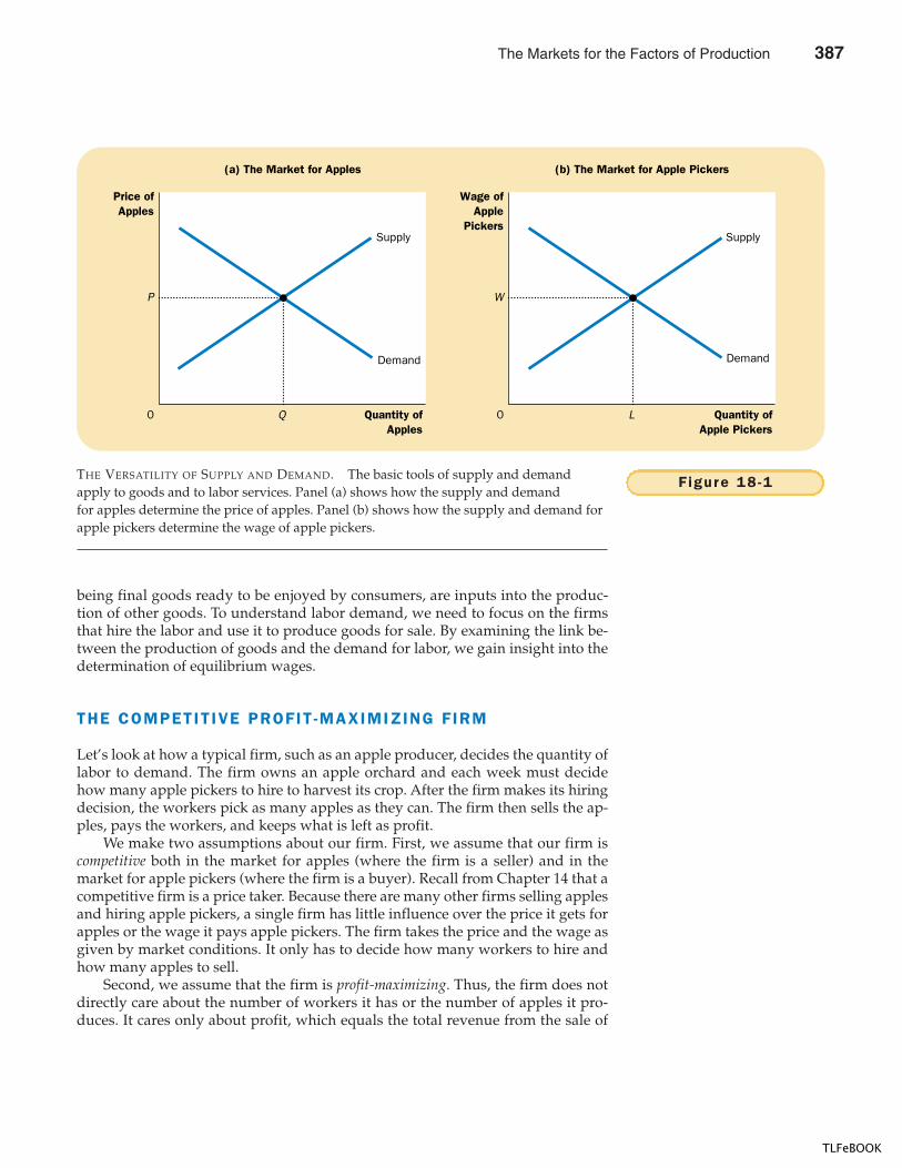
CHAPTER 18 THE MARKETS FOR THE FACTORS OF PRODUCTION 399
being final goods ready to be enjoyed by consumers, are inputs into the produc-tion of other goods. To understand labor demand, we need to focus on the firmsthat hire the labor and use it to produce goods for sale. By examining the link be-tween the production of goods and the demand for labor, we gain insight into thedetermination of equilibrium wages.
THE COMPETIT IVE PROFIT -MAXIMIZING F IRM
Let’s look at how a typical firm, such as an apple producer, decides the quantity oflabor to demand. The firm owns an apple orchard and each week must decidehow many apple pickers to hire to harvest its crop. After the firm makes its hiringdecision, the workers pick as many apples as they can. The firm then sells the ap-ples, pays the workers, and keeps what is left as profit.
We make two assumptions about our firm. First, we assume that our firm iscompetitive both in the market for apples (where the firm is a seller) and in themarket for apple pickers (where the firm is a buyer). Recall from Chapter 14 that acompetitive firm is a price taker. Because there are many other firms selling applesand hiring apple pickers, a single firm has little influence over the price it gets forapples or the wage it pays apple pickers. The firm takes the price and the wage asgiven by market conditions. It only has to decide how many workers to hire andhow many apples to sell.
Second, we assume that the firm is profit-maximizing. Thus, the firm does notdirectly care about the number of workers it has or the number of apples it pro-duces. It cares only about profit, which equals the total revenue from the sale of
Quantity ofApples
0
Price ofApples
P
Q
Demand
Supply
Demand
Supply
Quantity ofApple Pickers
0
Wage ofApple
Pickers
L
W
(a) The Market for Apples (b) The Market for Apple Pickers
F igure 18 -1THE VERSATILITY OF SUPPLY AND DEMAND. The basic tools of supply and demandapply to goods and to labor services. Panel (a) shows how the supply and demandfor apples determine the price of apples. Panel (b) shows how the supply and demand forapple pickers determine the wage of apple pickers.
The Markets for the Factors of Production 387
TLFeBOOK
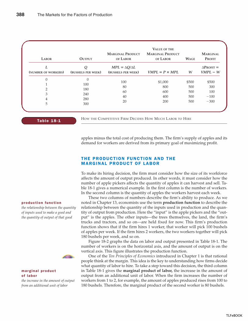
400 PART SIX THE ECONOMICS OF LABOR MARKETS
apples minus the total cost of producing them. The firm’s supply of apples and itsdemand for workers are derived from its primary goal of maximizing profit.
THE PRODUCTION FUNCTION AND THEMARGINAL PRODUCT OF LABOR
To make its hiring decision, the firm must consider how the size of its workforceaffects the amount of output produced. In other words, it must consider how thenumber of apple pickers affects the quantity of apples it can harvest and sell. Ta-ble 18-1 gives a numerical example. In the first column is the number of workers.In the second column is the quantity of apples the workers harvest each week.
These two columns of numbers describe the firm’s ability to produce. As wenoted in Chapter 13, economists use the term production function to describe therelationship between the quantity of the inputs used in production and the quan-tity of output from production. Here the “input” is the apple pickers and the “out-put” is the apples. The other inputs—the trees themselves, the land, the firm’strucks and tractors, and so on—are held fixed for now. This firm’s productionfunction shows that if the firm hires 1 worker, that worker will pick 100 bushelsof apples per week. If the firm hires 2 workers, the two workers together will pick180 bushels per week, and so on.
Figure 18-2 graphs the data on labor and output presented in Table 18-1. Thenumber of workers is on the horizontal axis, and the amount of output is on thevertical axis. This figure illustrates the production function.
One of the Ten Principles of Economics introduced in Chapter 1 is that rationalpeople think at the margin. This idea is the key to understanding how firms decidewhat quantity of labor to hire. To take a step toward this decision, the third columnin Table 18-1 gives the marginal product of labor, the increase in the amount ofoutput from an additional unit of labor. When the firm increases the number ofworkers from 1 to 2, for example, the amount of apples produced rises from 100 to180 bushels. Therefore, the marginal product of the second worker is 80 bushels.
Table 18 -1
VALUE OF THE
MARGINAL PRODUCT MARGINAL PRODUCT MARGINAL
LABOR OUTPUT OF LABOR OF LABOR WAGE PROFIT
L Q MPL � ∆Q/∆L ∆PROFIT �
(NUMBER OF WORKERS) (BUSHELS PER WEEK) (BUSHELS PER WEEK) VMPL � P � MPL W VMPL � W
0 0100 $1,000 $500 $500
1 10080 800 500 300
2 18060 600 500 100
3 24040 400 500 �100
4 28020 200 500 �300
5 300
HOW THE COMPETITIVE FIRM DECIDES HOW MUCH LABOR TO HIRE
product ion funct ionthe relationship between the quantityof inputs used to make a good andthe quantity of output of that good
marg ina l p roduct o f laborthe increase in the amount of outputfrom an additional unit of labor
388 The Markets for the Factors of Production
TLFeBOOK
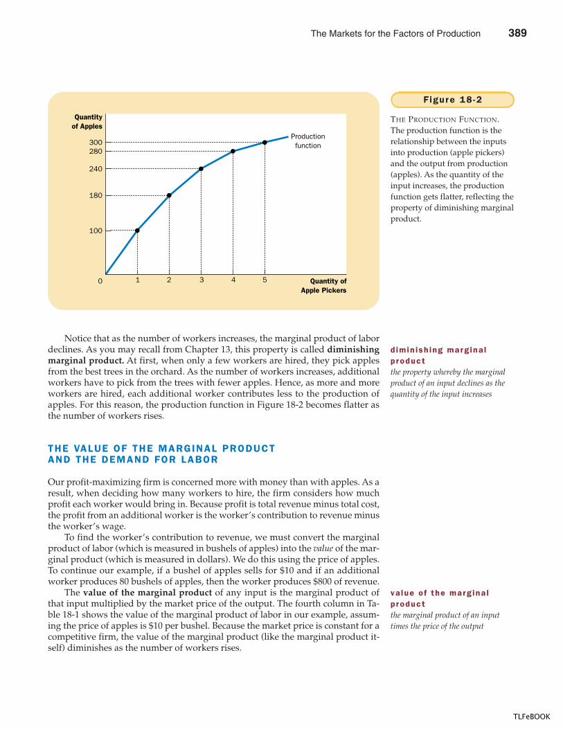
CHAPTER 18 THE MARKETS FOR THE FACTORS OF PRODUCTION 401
Notice that as the number of workers increases, the marginal product of labordeclines. As you may recall from Chapter 13, this property is called diminishingmarginal product. At first, when only a few workers are hired, they pick applesfrom the best trees in the orchard. As the number of workers increases, additionalworkers have to pick from the trees with fewer apples. Hence, as more and moreworkers are hired, each additional worker contributes less to the production ofapples. For this reason, the production function in Figure 18-2 becomes flatter asthe number of workers rises.
THE VALUE OF THE MARGINAL PRODUCTAND THE DEMAND FOR LABOR
Our profit-maximizing firm is concerned more with money than with apples. As aresult, when deciding how many workers to hire, the firm considers how muchprofit each worker would bring in. Because profit is total revenue minus total cost,the profit from an additional worker is the worker’s contribution to revenue minusthe worker’s wage.
To find the worker’s contribution to revenue, we must convert the marginalproduct of labor (which is measured in bushels of apples) into the value of the mar-ginal product (which is measured in dollars). We do this using the price of apples.To continue our example, if a bushel of apples sells for $10 and if an additionalworker produces 80 bushels of apples, then the worker produces $800 of revenue.
The value of the marginal product of any input is the marginal product ofthat input multiplied by the market price of the output. The fourth column in Ta-ble 18-1 shows the value of the marginal product of labor in our example, assum-ing the price of apples is $10 per bushel. Because the market price is constant for acompetitive firm, the value of the marginal product (like the marginal product it-self) diminishes as the number of workers rises.
d imin ish ing marg ina lproductthe property whereby the marginalproduct of an input declines as thequantity of the input increases
Quantity ofApple Pickers
0
Quantityof Apples
300280
240
180
100
Productionfunction
1 2 3 4 5
Figure 18 -2
THE PRODUCTION FUNCTION.The production function is therelationship between the inputsinto production (apple pickers)and the output from production(apples). As the quantity of theinput increases, the productionfunction gets flatter, reflecting theproperty of diminishing marginalproduct.
va lue o f the marg ina lproductthe marginal product of an inputtimes the price of the output
The Markets for the Factors of Production 389
TLFeBOOK
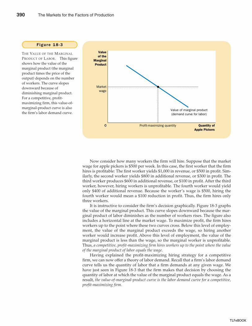
402 PART SIX THE ECONOMICS OF LABOR MARKETS
Now consider how many workers the firm will hire. Suppose that the marketwage for apple pickers is $500 per week. In this case, the first worker that the firmhires is profitable: The first worker yields $1,000 in revenue, or $500 in profit. Sim-ilarly, the second worker yields $800 in additional revenue, or $300 in profit. Thethird worker produces $600 in additional revenue, or $100 in profit. After the thirdworker, however, hiring workers is unprofitable. The fourth worker would yieldonly $400 of additional revenue. Because the worker’s wage is $500, hiring thefourth worker would mean a $100 reduction in profit. Thus, the firm hires onlythree workers.
It is instructive to consider the firm’s decision graphically. Figure 18-3 graphsthe value of the marginal product. This curve slopes downward because the mar-ginal product of labor diminishes as the number of workers rises. The figure alsoincludes a horizontal line at the market wage. To maximize profit, the firm hiresworkers up to the point where these two curves cross. Below this level of employ-ment, the value of the marginal product exceeds the wage, so hiring anotherworker would increase profit. Above this level of employment, the value of themarginal product is less than the wage, so the marginal worker is unprofitable.Thus, a competitive, profit-maximizing firm hires workers up to the point where the valueof the marginal product of labor equals the wage.
Having explained the profit-maximizing hiring strategy for a competitivefirm, we can now offer a theory of labor demand. Recall that a firm’s labor demandcurve tells us the quantity of labor that a firm demands at any given wage. Wehave just seen in Figure 18-3 that the firm makes that decision by choosing thequantity of labor at which the value of the marginal product equals the wage. As aresult, the value-of-marginal-product curve is the labor demand curve for a competitive,profit-maximizing firm.
0 Quantity ofApple Pickers
0
Value of the
MarginalProduct
Marketwage
Profit-maximizing quantity
Value of marginal product(demand curve for labor)
Figure 18 -3
THE VALUE OF THE MARGINAL
PRODUCT OF LABOR. This figureshows how the value of themarginal product (the marginalproduct times the price of theoutput) depends on the numberof workers. The curve slopesdownward because ofdiminishing marginal product.For a competitive, profit-maximizing firm, this value-of-marginal-product curve is alsothe firm’s labor demand curve.
390 The Markets for the Factors of Production
TLFeBOOK
CHAPTER 18 THE MARKETS FOR THE FACTORS OF PRODUCTION 403
WHAT CAUSES THE LABOR DEMAND CURVE TO SHIFT?
We now understand the labor demand curve: It is nothing more than a reflectionof the value of marginal product of labor. With this insight in mind, let’s considera few of the things that might cause the labor demand curve to shift.
The Output Pr ice The value of the marginal product is marginal producttimes the price of the firm’s output. Thus, when the output price changes, thevalue of the marginal product changes, and the labor demand curve shifts. An in-crease in the price of apples, for instance, raises the value of the marginal productof each worker that picks apples and, therefore, increases labor demand from thefirms that supply apples. Conversely, a decrease in the price of apples reduces thevalue of the marginal product and decreases labor demand.
Techno log ica l Change Between 1968 and 1998, the amount of outputa typical U.S. worker produced in an hour rose by 57 percent. Why? The most
In Chapter 14 we saw howa competitive, profit-maximizingfirm decides how much of itsoutput to sell: It chooses thequantity of output at which theprice of the good equals themarginal cost of production. Wehave just seen how such a firmdecides how much labor tohire: It chooses the quantity oflabor at which the wage equalsthe value of the marginal prod-uct. Because the production
function links the quantity of inputs to the quantity of output,you should not be surprised to learn that the firm’s decisionabout input demand is closely linked to its decision aboutoutput supply. In fact, these two decisions are two sides ofthe same coin.
To see this relationship more fully, let’s consider howthe marginal product of labor (MPL) and marginal cost (MC)are related. Suppose an additional worker costs $500 andhas a marginal product of 50 bushels of apples. In thiscase, producing 50 more bushels costs $500; the marginalcost of a bushel is $500/50, or $10. More generally, if Wis the wage, and an extra unit of labor produces MPL unitsof output, then the marginal cost of a unit of output isMC � W/MPL.
This analysis shows that diminishing marginal productis closely related to increasing marginal cost. When our ap-ple orchard grows crowded with workers, each additional
worker adds less to the production of apples (MPL falls).Similarly, when the apple firm is producing a large quantityof apples, the orchard is already crowded with workers, so itis more costly to produce an additional bushel of apples(MC rises).
Now consider our criterion for profit maximization. Wedetermined earlier that a profit-maximizing firm chooses thequantity of labor so that the value of the marginal product(P � MPL) equals the wage (W). We can write this mathe-matically as
P � MPL � W.
If we divide both sides of this equation by MPL, we obtain
P � W/MPL.
We just noted that W/MPL equals marginal cost MC. There-fore, we can substitute to obtain
P � MC.
This equation states that the price of the firm’s output isequal to the marginal cost of producing a unit of output.Thus, when a competitive firm hires labor up to the point atwhich the value of the marginal product equals the wage, italso produces up to the point at which the price equals mar-ginal cost. Our analysis of labor demand in this chapter isjust another way of looking at the production decision wefirst saw in Chapter 14.
FYIInput Demand
and OutputSupply: TwoSides of theSame Coin
The Markets for the Factors of Production 391
TLFeBOOK
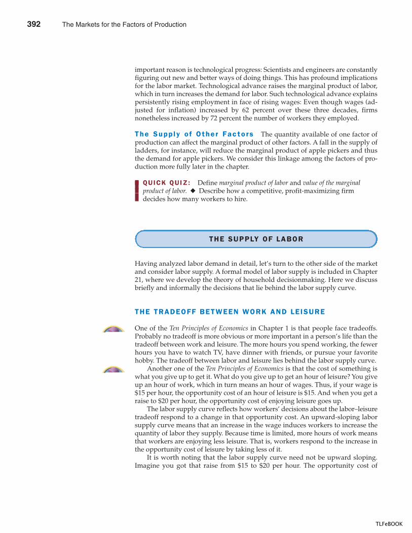
404 PART SIX THE ECONOMICS OF LABOR MARKETS
important reason is technological progress: Scientists and engineers are constantlyfiguring out new and better ways of doing things. This has profound implicationsfor the labor market. Technological advance raises the marginal product of labor,which in turn increases the demand for labor. Such technological advance explainspersistently rising employment in face of rising wages: Even though wages (ad-justed for inflation) increased by 62 percent over these three decades, firmsnonetheless increased by 72 percent the number of workers they employed.
The Supp ly o f Other Facto rs The quantity available of one factor ofproduction can affect the marginal product of other factors. A fall in the supply ofladders, for instance, will reduce the marginal product of apple pickers and thusthe demand for apple pickers. We consider this linkage among the factors of pro-duction more fully later in the chapter.
QUICK QUIZ: Define marginal product of labor and value of the marginal product of labor. � Describe how a competitive, profit-maximizing firm decides how many workers to hire.
THE SUPPLY OF LABOR
Having analyzed labor demand in detail, let’s turn to the other side of the marketand consider labor supply. A formal model of labor supply is included in Chapter21, where we develop the theory of household decisionmaking. Here we discussbriefly and informally the decisions that lie behind the labor supply curve.
THE TRADEOFF BETWEEN WORK AND LEISURE
One of the Ten Principles of Economics in Chapter 1 is that people face tradeoffs.Probably no tradeoff is more obvious or more important in a person’s life than thetradeoff between work and leisure. The more hours you spend working, the fewerhours you have to watch TV, have dinner with friends, or pursue your favoritehobby. The tradeoff between labor and leisure lies behind the labor supply curve.
Another one of the Ten Principles of Economics is that the cost of something iswhat you give up to get it. What do you give up to get an hour of leisure? You giveup an hour of work, which in turn means an hour of wages. Thus, if your wage is$15 per hour, the opportunity cost of an hour of leisure is $15. And when you get araise to $20 per hour, the opportunity cost of enjoying leisure goes up.
The labor supply curve reflects how workers’ decisions about the labor–leisuretradeoff respond to a change in that opportunity cost. An upward-sloping laborsupply curve means that an increase in the wage induces workers to increase thequantity of labor they supply. Because time is limited, more hours of work meansthat workers are enjoying less leisure. That is, workers respond to the increase inthe opportunity cost of leisure by taking less of it.
It is worth noting that the labor supply curve need not be upward sloping.Imagine you got that raise from $15 to $20 per hour. The opportunity cost of
392 The Markets for the Factors of Production
TLFeBOOK
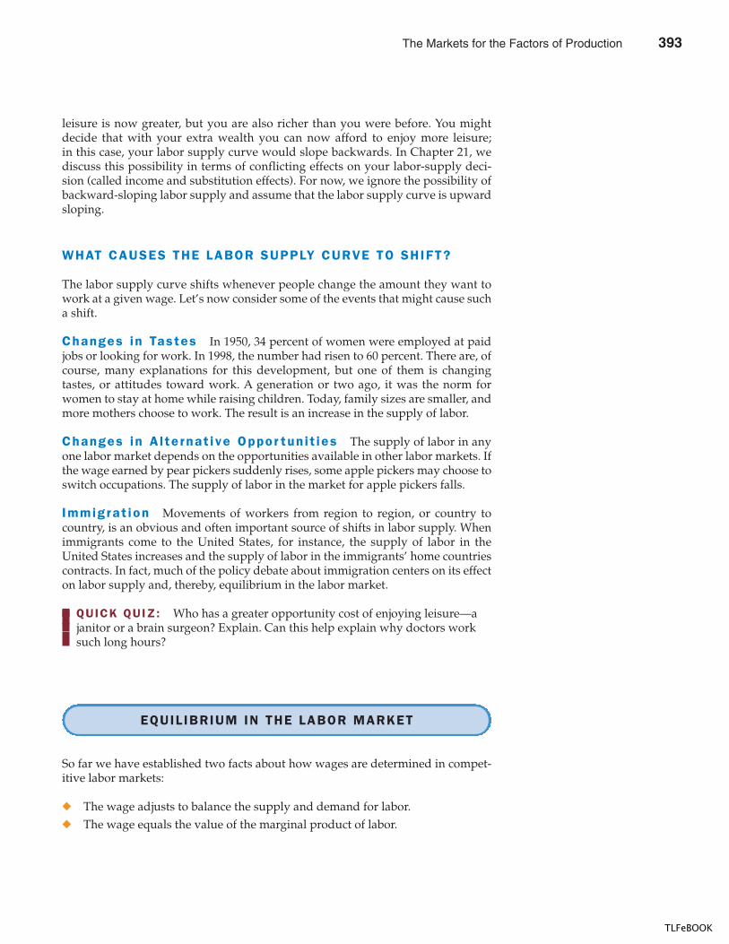
CHAPTER 18 THE MARKETS FOR THE FACTORS OF PRODUCTION 405
leisure is now greater, but you are also richer than you were before. You mightdecide that with your extra wealth you can now afford to enjoy more leisure;in this case, your labor supply curve would slope backwards. In Chapter 21, wediscuss this possibility in terms of conflicting effects on your labor-supply deci-sion (called income and substitution effects). For now, we ignore the possibility ofbackward-sloping labor supply and assume that the labor supply curve is upwardsloping.
WHAT CAUSES THE LABOR SUPPLY CURVE TO SHIFT?
The labor supply curve shifts whenever people change the amount they want towork at a given wage. Let’s now consider some of the events that might cause sucha shift.
Changes in Tastes In 1950, 34 percent of women were employed at paidjobs or looking for work. In 1998, the number had risen to 60 percent. There are, ofcourse, many explanations for this development, but one of them is changingtastes, or attitudes toward work. A generation or two ago, it was the norm forwomen to stay at home while raising children. Today, family sizes are smaller, andmore mothers choose to work. The result is an increase in the supply of labor.
Changes in A l te rnat ive Oppor tun i t ies The supply of labor in anyone labor market depends on the opportunities available in other labor markets. Ifthe wage earned by pear pickers suddenly rises, some apple pickers may choose toswitch occupations. The supply of labor in the market for apple pickers falls.
Immigrat ion Movements of workers from region to region, or country tocountry, is an obvious and often important source of shifts in labor supply. Whenimmigrants come to the United States, for instance, the supply of labor in theUnited States increases and the supply of labor in the immigrants’ home countriescontracts. In fact, much of the policy debate about immigration centers on its effecton labor supply and, thereby, equilibrium in the labor market.
QUICK QUIZ: Who has a greater opportunity cost of enjoying leisure—a janitor or a brain surgeon? Explain. Can this help explain why doctors work such long hours?
EQUIL IBRIUM IN THE LABOR MARKET
So far we have established two facts about how wages are determined in compet-itive labor markets:
� The wage adjusts to balance the supply and demand for labor.� The wage equals the value of the marginal product of labor.
The Markets for the Factors of Production 393
TLFeBOOK
406 PART SIX THE ECONOMICS OF LABOR MARKETS
At first, it might seem surprising that the wage can do both these things at once. Infact, there is no real puzzle here, but understanding why there is no puzzle is animportant step to understanding wage determination.
Figure 18-4 shows the labor market in equilibrium. The wage and the quantityof labor have adjusted to balance supply and demand. When the market is in thisequilibrium, each firm has bought as much labor as it finds profitable at the equi-librium wage. That is, each firm has followed the rule for profit maximization: Ithas hired workers until the value of the marginal product equals the wage. Hence,the wage must equal the value of marginal product of labor once it has broughtsupply and demand into equilibrium.
This brings us to an important lesson: Any event that changes the supply or de-mand for labor must change the equilibrium wage and the value of the marginal product bythe same amount, because these must always be equal. To see how this works, let’s con-sider some events that shift these curves.
SHIFTS IN LABOR SUPPLY
Suppose that immigration increases the number of workers willing to pick apples.As Figure 18-5 shows, the supply of labor shifts to the right from S1 to S2. At theinitial wage W1, the quantity of labor supplied now exceeds the quantity de-manded. This surplus of labor puts downward pressure on the wage of apple pick-ers, and the fall in the wage from W1 to W2 in turn makes it profitable for firms tohire more workers. As the number of workers employed in each apple orchardrises, the marginal product of a worker falls, and so does the value of the marginalproduct. In the new equilibrium, both the wage and the value of the marginalproduct of labor are lower than they were before the influx of new workers.
Wage(price of
labor)
Equilibriumwage, W
0 Quantity ofLabor
Equilibriumemployment, L
Supply
Demand
Figure 18 -4
EQUILIBRIUM IN A LABOR
MARKET. Like all prices, theprice of labor (the wage) dependson supply and demand. Becausethe demand curve reflects thevalue of the marginal product oflabor, in equilibrium workersreceive the value of theirmarginal contribution to theproduction of goods and services.
394 The Markets for the Factors of Production
TLFeBOOK
CHAPTER 18 THE MARKETS FOR THE FACTORS OF PRODUCTION 407
An episode from Israel illustrates how a shift in labor supply can alter theequilibrium in a labor market. During most of the 1980s, many thousands of Pale-stinians regularly commuted from their homes in the Israeli-occupied West Bankand Gaza Strip to jobs in Israel, primarily in the construction and agricultureindustries. In 1988, however, political unrest in these occupied areas induced theIsraeli government to take steps that, as a by-product, reduced this supply ofworkers. Curfews were imposed, work permits were checked more thoroughly,and a ban on overnight stays of Palestinians in Israel was enforced more rigor-ously. The economic impact of these steps was exactly as theory predicts: Thenumber of Palestinians with jobs in Israel fell by half, while those who continuedto work in Israel enjoyed wage increases of about 50 percent. With a reduced num-ber of Palestinian workers in Israel, the value of the marginal product of the re-maining workers was much higher.
SHIFTS IN LABOR DEMAND
Now suppose that an increase in the popularity of apples causes their price to rise.This price increase does not change the marginal product of labor for any givennumber of workers, but it does raise the value of the marginal product. With ahigher price of apples, hiring more apple pickers is now profitable. As Figure 18-6shows, when the demand for labor shifts to the right from D1 to D2, the equilib-rium wage rises from W1 to W2, and equilibrium employment rises from L1 to L2.Once again, the wage and the value of the marginal product of labor movetogether.
This analysis shows that prosperity for firms in an industry is often linkedto prosperity for workers in that industry. When the price of apples rises, apple
Wage(price of
labor)
W2
W1
0 Quantity ofLabor
L2L1
Supply, S1
Demand
2. . . . reducesthe wage . . .
3. . . . and raises employment.
1. An increase inlabor supply . . .
S2
Figure 18 -5
A SHIFT IN LABOR SUPPLY.When labor supply increasesfrom S1 to S2, perhaps because ofan immigration of new workers,the equilibrium wage falls fromW1 to W2. At this lower wage,firms hire more labor, soemployment rises from L1 to L2.The change in the wage reflects achange in the value of themarginal product of labor: Withmore workers, the added outputfrom an extra worker is smaller.
The Markets for the Factors of Production 395
TLFeBOOK
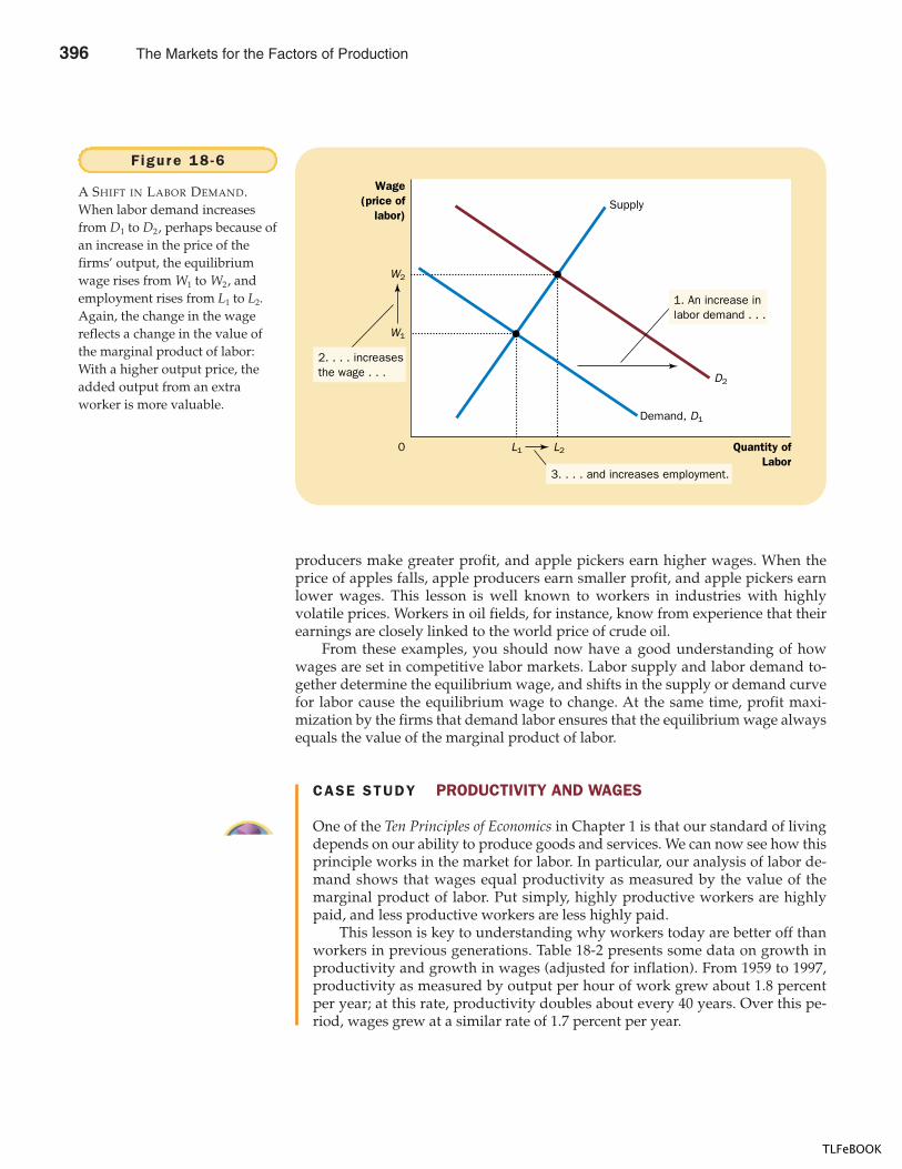
408 PART SIX THE ECONOMICS OF LABOR MARKETS
CASE STUDY PRODUCTIVITY AND WAGES
One of the Ten Principles of Economics in Chapter 1 is that our standard of livingdepends on our ability to produce goods and services. We can now see how thisprinciple works in the market for labor. In particular, our analysis of labor de-mand shows that wages equal productivity as measured by the value of themarginal product of labor. Put simply, highly productive workers are highlypaid, and less productive workers are less highly paid.
This lesson is key to understanding why workers today are better off thanworkers in previous generations. Table 18-2 presents some data on growth inproductivity and growth in wages (adjusted for inflation). From 1959 to 1997,productivity as measured by output per hour of work grew about 1.8 percentper year; at this rate, productivity doubles about every 40 years. Over this pe-riod, wages grew at a similar rate of 1.7 percent per year.
producers make greater profit, and apple pickers earn higher wages. When theprice of apples falls, apple producers earn smaller profit, and apple pickers earnlower wages. This lesson is well known to workers in industries with highlyvolatile prices. Workers in oil fields, for instance, know from experience that theirearnings are closely linked to the world price of crude oil.
From these examples, you should now have a good understanding of howwages are set in competitive labor markets. Labor supply and labor demand to-gether determine the equilibrium wage, and shifts in the supply or demand curvefor labor cause the equilibrium wage to change. At the same time, profit maxi-mization by the firms that demand labor ensures that the equilibrium wage alwaysequals the value of the marginal product of labor.
Wage(price of
labor)
W1
W2
0 Quantity ofLabor
L1 L2
Supply
Demand, D1
2. . . . increasesthe wage . . .
3. . . . and increases employment.
1. An increase inlabor demand . . .
D2
Figure 18 -6
A SHIFT IN LABOR DEMAND.When labor demand increasesfrom D1 to D2, perhaps because ofan increase in the price of thefirms’ output, the equilibriumwage rises from W1 to W2, andemployment rises from L1 to L2.Again, the change in the wagereflects a change in the value ofthe marginal product of labor:With a higher output price, theadded output from an extraworker is more valuable.
396 The Markets for the Factors of Production
TLFeBOOK
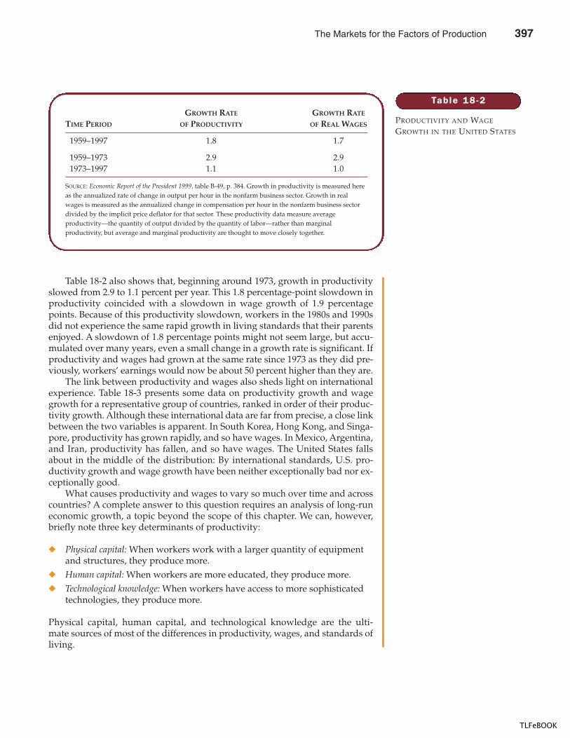
CHAPTER 18 THE MARKETS FOR THE FACTORS OF PRODUCTION 409
Table 18-2 also shows that, beginning around 1973, growth in productivityslowed from 2.9 to 1.1 percent per year. This 1.8 percentage-point slowdown inproductivity coincided with a slowdown in wage growth of 1.9 percentagepoints. Because of this productivity slowdown, workers in the 1980s and 1990sdid not experience the same rapid growth in living standards that their parentsenjoyed. A slowdown of 1.8 percentage points might not seem large, but accu-mulated over many years, even a small change in a growth rate is significant. Ifproductivity and wages had grown at the same rate since 1973 as they did pre-viously, workers’ earnings would now be about 50 percent higher than they are.
The link between productivity and wages also sheds light on internationalexperience. Table 18-3 presents some data on productivity growth and wagegrowth for a representative group of countries, ranked in order of their produc-tivity growth. Although these international data are far from precise, a close linkbetween the two variables is apparent. In South Korea, Hong Kong, and Singa-pore, productivity has grown rapidly, and so have wages. In Mexico, Argentina,and Iran, productivity has fallen, and so have wages. The United States fallsabout in the middle of the distribution: By international standards, U.S. pro-ductivity growth and wage growth have been neither exceptionally bad nor ex-ceptionally good.
What causes productivity and wages to vary so much over time and acrosscountries? A complete answer to this question requires an analysis of long-runeconomic growth, a topic beyond the scope of this chapter. We can, however,briefly note three key determinants of productivity:
� Physical capital: When workers work with a larger quantity of equipmentand structures, they produce more.
� Human capital: When workers are more educated, they produce more.� Technological knowledge: When workers have access to more sophisticated
technologies, they produce more.
Physical capital, human capital, and technological knowledge are the ulti-mate sources of most of the differences in productivity, wages, and standards ofliving.
Table 18 -2
PRODUCTIVITY AND WAGE
GROWTH IN THE UNITED STATES
GROWTH RATE GROWTH RATE
TIME PERIOD OF PRODUCTIVITY OF REAL WAGES
1959–1997 1.8 1.7
1959–1973 2.9 2.91973–1997 1.1 1.0
SOURCE: Economic Report of the President 1999, table B-49, p. 384. Growth in productivity is measured hereas the annualized rate of change in output per hour in the nonfarm business sector. Growth in realwages is measured as the annualized change in compensation per hour in the nonfarm business sectordivided by the implicit price deflator for that sector. These productivity data measure averageproductivity—the quantity of output divided by the quantity of labor—rather than marginalproductivity, but average and marginal productivity are thought to move closely together.
The Markets for the Factors of Production 397
TLFeBOOK
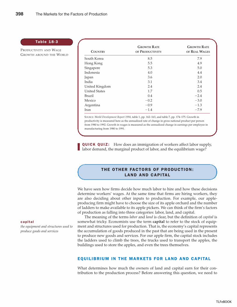
410 PART SIX THE ECONOMICS OF LABOR MARKETS
QUICK QUIZ: How does an immigration of workers affect labor supply, labor demand, the marginal product of labor, and the equilibrium wage?
THE OTHER FACTORS OF PRODUCTION:LAND AND CAPITAL
We have seen how firms decide how much labor to hire and how these decisionsdetermine workers’ wages. At the same time that firms are hiring workers, theyare also deciding about other inputs to production. For example, our apple-producing firm might have to choose the size of its apple orchard and the numberof ladders to make available to its apple pickers. We can think of the firm’s factorsof production as falling into three categories: labor, land, and capital.
The meaning of the terms labor and land is clear, but the definition of capital issomewhat tricky. Economists use the term capital to refer to the stock of equip-ment and structures used for production. That is, the economy’s capital representsthe accumulation of goods produced in the past that are being used in the presentto produce new goods and services. For our apple firm, the capital stock includesthe ladders used to climb the trees, the trucks used to transport the apples, thebuildings used to store the apples, and even the trees themselves.
EQUIL IBRIUM IN THE MARKETS FOR LAND AND CAPITAL
What determines how much the owners of land and capital earn for their con-tribution to the production process? Before answering this question, we need to
Table 18 -3
PRODUCTIVITY AND WAGE
GROWTH AROUND THE WORLD
GROWTH RATE GROWTH RATE
COUNTRY OF PRODUCTIVITY OF REAL WAGES
South Korea 8.5 7.9Hong Kong 5.5 4.9Singapore 5.3 5.0Indonesia 4.0 4.4Japan 3.6 2.0India 3.1 3.4United Kingdom 2.4 2.4United States 1.7 0.5Brazil 0.4 �2.4Mexico �0.2 �3.0Argentina �0.9 �1.3Iran �1.4 �7.9
SOURCE: World Development Report 1994, table 1, pp. 162–163, and table 7, pp. 174–175. Growth inproductivity is measured here as the annualized rate of change in gross national product per personfrom 1980 to 1992. Growth in wages is measured as the annualized change in earnings per employee inmanufacturing from 1980 to 1991.
capi ta lthe equipment and structures used toproduce goods and services
398 The Markets for the Factors of Production
TLFeBOOK
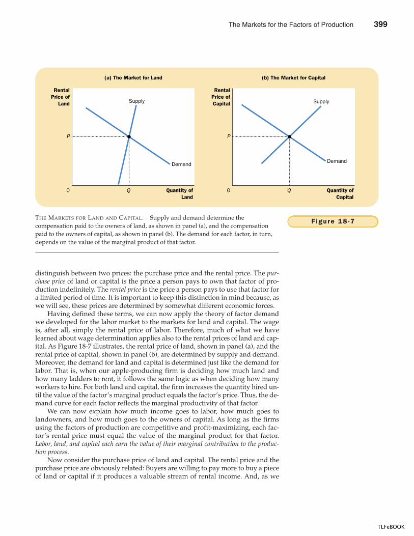
CHAPTER 18 THE MARKETS FOR THE FACTORS OF PRODUCTION 411
distinguish between two prices: the purchase price and the rental price. The pur-chase price of land or capital is the price a person pays to own that factor of pro-duction indefinitely. The rental price is the price a person pays to use that factor fora limited period of time. It is important to keep this distinction in mind because, aswe will see, these prices are determined by somewhat different economic forces.
Having defined these terms, we can now apply the theory of factor demandwe developed for the labor market to the markets for land and capital. The wageis, after all, simply the rental price of labor. Therefore, much of what we havelearned about wage determination applies also to the rental prices of land and cap-ital. As Figure 18-7 illustrates, the rental price of land, shown in panel (a), and therental price of capital, shown in panel (b), are determined by supply and demand.Moreover, the demand for land and capital is determined just like the demand forlabor. That is, when our apple-producing firm is deciding how much land andhow many ladders to rent, it follows the same logic as when deciding how manyworkers to hire. For both land and capital, the firm increases the quantity hired un-til the value of the factor’s marginal product equals the factor’s price. Thus, the de-mand curve for each factor reflects the marginal productivity of that factor.
We can now explain how much income goes to labor, how much goes tolandowners, and how much goes to the owners of capital. As long as the firmsusing the factors of production are competitive and profit-maximizing, each fac-tor’s rental price must equal the value of the marginal product for that factor.Labor, land, and capital each earn the value of their marginal contribution to the produc-tion process.
Now consider the purchase price of land and capital. The rental price and thepurchase price are obviously related: Buyers are willing to pay more to buy a pieceof land or capital if it produces a valuable stream of rental income. And, as we
Quantity ofLand
0
RentalPrice of
Land
P
Q
Demand
Supply
Demand
Supply
Quantity ofCapital
0
RentalPrice ofCapital
Q
P
(a) The Market for Land (b) The Market for Capital
F igure 18 -7THE MARKETS FOR LAND AND CAPITAL. Supply and demand determine thecompensation paid to the owners of land, as shown in panel (a), and the compensationpaid to the owners of capital, as shown in panel (b). The demand for each factor, in turn,depends on the value of the marginal product of that factor.
The Markets for the Factors of Production 399
TLFeBOOK
412 PART SIX THE ECONOMICS OF LABOR MARKETS
have just seen, the equilibrium rental income at any point in time equals the valueof that factor’s marginal product. Therefore, the equilibrium purchase price of apiece of land or capital depends on both the current value of the marginal productand the value of the marginal product expected to prevail in the future.
LINKAGES AMONG THE FACTORS OF PRODUCTION
We have seen that the price paid to any factor of production—labor, land, or capi-tal—equals the value of the marginal product of that factor. The marginal productof any factor, in turn, depends on the quantity of that factor that is available. Be-cause of diminishing returns, a factor in abundant supply has a low marginalproduct and thus a low price, and a factor in scarce supply has a high marginalproduct and a high price. As a result, when the supply of a factor falls, its equilib-rium factor price rises.
When the supply of any factor changes, however, the effects are not limited tothe market for that factor. In most situations, factors of production are used to-gether in a way that makes the productivity of each factor dependent on the quan-tities of the other factors available to be used in the production process. As a result,a change in the supply of any one factor alters the earnings of all the factors.
For example, suppose that a hurricane destroys many of the ladders thatworkers use to pick apples from the orchards. What happens to the earnings of thevarious factors of production? Most obviously, the supply of ladders falls and,
Labor income is an easy con-cept to understand: It is thepaycheck that workers get fromtheir employers. The incomeearned by capital, however, isless obvious.
In our analysis, we havebeen implicitly assuming thathouseholds own the economy’sstock of capital—ladders, drillpresses, warehouses, etc.—and rent it to the firms that useit. Capital income, in this case,
is the rent that households receive for the use of their capi-tal. This assumption simplified our analysis of how capitalowners are compensated, but it is not entirely realistic. Infact, firms usually own the capital they use and, therefore,they receive the earnings from this capital.
These earnings from capital, however, eventually getpaid to households. Some of the earnings are paid in theform of interest to those households who have lent moneyto firms. Bondholders and bank depositors are two exam-ples of recipients of interest. Thus, when you receive inter-
est on your bank account, that income is part of the econ-omy’s capital income.
In addition, some of the earnings from capital are paidto households in the form of dividends. Dividends are pay-ments by a firm to the firm’s stockholders. A stockholder isa person who has bought a share in the ownership of thefirm and, therefore, is entitled to share in the firm’s profits.
A firm does not have to pay out all of its earnings tohouseholds in the form of interest and dividends. Instead, itcan retain some earnings within the firm and use theseearnings to buy additional capital. Although these retainedearnings do not get paid to the firm’s stockholders, thestockholders benefit from them nonetheless. Because re-tained earnings increase the amount of capital the firmowns, they tend to increase future earnings and, thereby,the value of the firm’s stock.
These institutional details are interesting and impor-tant, but they do not alter our conclusion about the incomeearned by the owners of capital. Capital is paid according tothe value of its marginal product, regardless of whether thisincome gets transmitted to households in the form of inter-est or dividends or whether it is kept within firms as re-tained earnings.
FYI
What Is
Capital Income?
400 The Markets for the Factors of Production
TLFeBOOK
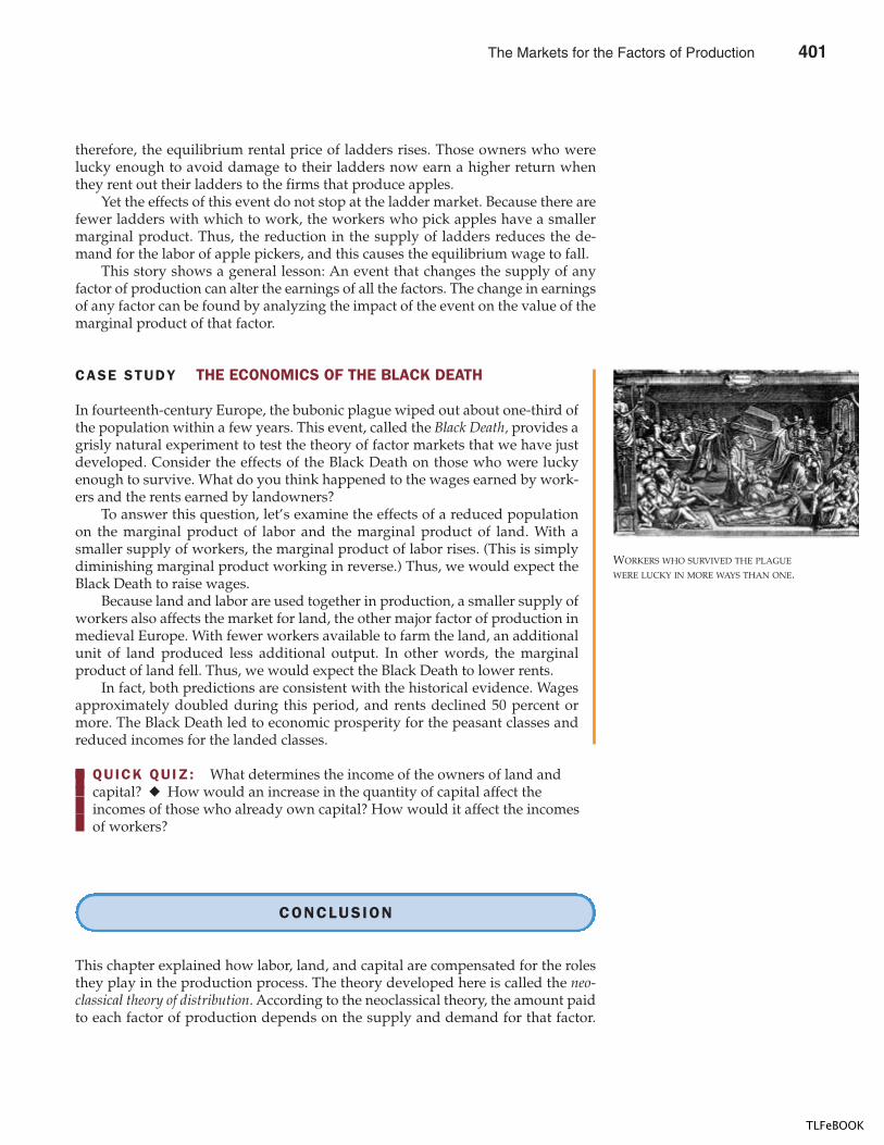
CHAPTER 18 THE MARKETS FOR THE FACTORS OF PRODUCTION 413
CASE STUDY THE ECONOMICS OF THE BLACK DEATH
In fourteenth-century Europe, the bubonic plague wiped out about one-third ofthe population within a few years. This event, called the Black Death, provides agrisly natural experiment to test the theory of factor markets that we have justdeveloped. Consider the effects of the Black Death on those who were luckyenough to survive. What do you think happened to the wages earned by work-ers and the rents earned by landowners?
To answer this question, let’s examine the effects of a reduced populationon the marginal product of labor and the marginal product of land. With asmaller supply of workers, the marginal product of labor rises. (This is simplydiminishing marginal product working in reverse.) Thus, we would expect theBlack Death to raise wages.
Because land and labor are used together in production, a smaller supply ofworkers also affects the market for land, the other major factor of production inmedieval Europe. With fewer workers available to farm the land, an additionalunit of land produced less additional output. In other words, the marginalproduct of land fell. Thus, we would expect the Black Death to lower rents.
In fact, both predictions are consistent with the historical evidence. Wagesapproximately doubled during this period, and rents declined 50 percent ormore. The Black Death led to economic prosperity for the peasant classes andreduced incomes for the landed classes.
therefore, the equilibrium rental price of ladders rises. Those owners who werelucky enough to avoid damage to their ladders now earn a higher return whenthey rent out their ladders to the firms that produce apples.
Yet the effects of this event do not stop at the ladder market. Because there arefewer ladders with which to work, the workers who pick apples have a smallermarginal product. Thus, the reduction in the supply of ladders reduces the de-mand for the labor of apple pickers, and this causes the equilibrium wage to fall.
This story shows a general lesson: An event that changes the supply of anyfactor of production can alter the earnings of all the factors. The change in earningsof any factor can be found by analyzing the impact of the event on the value of themarginal product of that factor.
WORKERS WHO SURVIVED THE PLAGUE
WERE LUCKY IN MORE WAYS THAN ONE.
QUICK QUIZ: What determines the income of the owners of land and capital? � How would an increase in the quantity of capital affect the incomes of those who already own capital? How would it affect the incomes of workers?
CONCLUSION
This chapter explained how labor, land, and capital are compensated for the rolesthey play in the production process. The theory developed here is called the neo-classical theory of distribution. According to the neoclassical theory, the amount paidto each factor of production depends on the supply and demand for that factor.
The Markets for the Factors of Production 401
TLFeBOOK
414 PART SIX THE ECONOMICS OF LABOR MARKETS
The demand, in turn, depends on that particular factor’s marginal productivity. Inequilibrium, each factor of production earns the value of its marginal contributionto the production of goods and services.
The neoclassical theory of distribution is widely accepted. Most economistsbegin with the neoclassical theory when trying to explain how the U.S. economy’s$8 trillion of income is distributed among the economy’s various members. In thefollowing two chapters, we consider the distribution of income in more detail. Asyou will see, the neoclassical theory provides the framework for this discussion.
Even at this point you can use the theory to answer the question that beganthis chapter: Why are computer programmers paid more than gas station atten-dants? It is because programmers can produce a good of greater market value thancan a gas station attendant. People are willing to pay dearly for a good computergame, but they are willing to pay little to have their gas pumped and their wind-shield washed. The wages of these workers reflect the market prices of the goodsthey produce. If people suddenly got tired of using computers and decided tospend more time driving, the prices of these goods would change, and so wouldthe equilibrium wages of these two groups of workers.
� The economy’s income is distributed in the markets forthe factors of production. The three most importantfactors of production are labor, land, and capital.
� The demand for factors, such as labor, is a deriveddemand that comes from firms that use the factors toproduce goods and services. Competitive, profit-maximizing firms hire each factor up to the point atwhich the value of the marginal product of the factorequals its price.
� The supply of labor arises from individuals’ tradeoffbetween work and leisure. An upward-sloping laborsupply curve means that people respond to an increasein the wage by enjoying less leisure and working morehours.
� The price paid to each factor adjusts to balance thesupply and demand for that factor. Because factordemand reflects the value of the marginal product ofthat factor, in equilibrium each factor is compensatedaccording to its marginal contribution to the productionof goods and services.
� Because factors of production are used together, themarginal product of any one factor depends on thequantities of all factors that are available. As a result, achange in the supply of one factor alters the equilibriumearnings of all the factors.
Summar y
factors of production, p. 398production function, p. 400
marginal product of labor, p. 400diminishing marginal product, p. 401
value of the marginal product, p. 401capital, p. 410
Key Concepts
1. Explain how a firm’s production function is relatedto its marginal product of labor, how a firm’smarginal product of labor is related to the value
of its marginal product, and how a firm’s valueof marginal product is related to its demand forlabor.
Quest ions fo r Rev iew
402 The Markets for the Factors of Production
TLFeBOOK
CHAPTER 18 THE MARKETS FOR THE FACTORS OF PRODUCTION 415
2. Give two examples of events that could shift thedemand for labor.
3. Give two examples of events that could shift the supplyof labor.
4. Explain how the wage can adjust to balance the supplyand demand for labor while simultaneously equalingthe value of the marginal product of labor.
5. If the population of the United States suddenly grewbecause of a large immigration, what would happen towages? What would happen to the rents earned by theowners of land and capital?
1. Suppose that the president proposes a new law aimed atreducing heath care costs: All Americans are to berequired to eat one apple daily.a. How would this apple-a-day law affect the demand
and equilibrium price of apples?b. How would the law affect the marginal product
and the value of the marginal product of applepickers?
c. How would the law affect the demand andequilibrium wage for apple pickers?
2. Henry Ford once said: “It is not the employer who payswages—he only handles the money. It is the productthat pays wages.” Explain.
3. Show the effect of each of the following events on themarket for labor in the computer manufacturingindustry.a. Congress buys personal computers for all American
college students.b. More college students major in engineering and
computer science.c. Computer firms build new manufacturing plants.
4. Your enterprising uncle opens a sandwich shop thatemploys 7 people. The employees are paid $6 per hour,and a sandwich sells for $3. If your uncle is maximizinghis profit, what is the value of the marginal product ofthe last worker he hired? What is that worker’smarginal product?
5. Imagine a firm that hires two types of workers—somewith computer skills and some without. If technologyadvances, so that computers become more useful to thefirm, what happens to the marginal product of the twotypes? What happens to equilibrium wages? Explain,using appropriate diagrams.
6. Suppose a freeze in Florida destroys part of the Floridaorange crop.a. Explain what happens to the price of oranges and
the marginal product of orange pickers as a result
of the freeze. Can you say what happens to thedemand for orange pickers? Why or why not?
b. Suppose the price of oranges doubles and themarginal product falls by 30 percent. What happensto the equilibrium wage of orange pickers?
c. Suppose the price of oranges rises by 30 percentand the marginal product falls by 50 percent.What happens to the equilibrium wage of orangepickers?
7. During the 1980s and 1990s the United Statesexperienced a significant inflow of capital from othercountries. For example, Toyota, BMW, and otherforeign car companies built auto plants in the UnitedStates.a. Using a diagram of the U.S. capital market, show
the effect of this inflow on the rental price of capitalin the United States and on the quantity of capitalin use.
b. Using a diagram of the U.S. labor market, show theeffect of the capital inflow on the average wagepaid to U.S. workers.
8. Suppose that labor is the only input used by a perfectlycompetitive firm that can hire workers for $50 per day.The firm’s production function is as follows:
DAYS OF LABOR UNITS OF OUTPUT
0 01 72 133 194 255 286 29
Each unit of output sells for $10. Plot the firm’s demandfor labor. How many days of labor should the firm hire?Show this point on your graph.
Prob lems and App l icat ions
The Markets for the Factors of Production 403
TLFeBOOK
416 PART SIX THE ECONOMICS OF LABOR MARKETS
9. (This question is challenging.) In recent years somepolicymakers have proposed requiring firms to giveworkers certain fringe benefits. For example, in 1993President Clinton proposed requiring firms to providehealth insurance to their workers. Let’s consider theeffects of such a policy on the labor market.a. Suppose that a law required firms to give each
worker $3 of fringe benefits for every hour that theworker is employed by the firm. How does this lawaffect the marginal profit that a firm earns fromeach worker? How does the law affect the demandcurve for labor? Draw your answer on a graph withthe cash wage on the vertical axis.
b. If there is no change in labor supply, how wouldthis law affect employment and wages?
c. Why might the labor supply curve shift in responseto this law? Would this shift in labor supply raise orlower the impact of the law on wages andemployment?
d. As Chapter 6 discussed, the wages of someworkers, particularly the unskilled and
inexperienced, are kept above the equilibrium levelby minimum-wage laws. What effect would afringe-benefit mandate have for these workers?
10. (This question is challenging.) This chapter has assumedthat labor is supplied by individual workers actingcompetitively. In some markets, however, the supply oflabor is determined by a union of workers.a. Explain why the situation faced by a labor union
may resemble the situation faced by a monopolyfirm.
b. The goal of a monopoly firm is to maximize profits.Is there an analogous goal for labor unions?
c. Now extend the analogy between monopoly firmsand unions. How do you suppose that the wage setby a union compares to the wage in a competitivemarket? How do you suppose employment differsin the two cases?
d. What other goals might unions have that makeunions different from monopoly firms?
404 The Markets for the Factors of Production
TLFeBOOK
IN THIS CHAPTERYOU WILL . . .
Cons ider why i t i sd i f f icu l t to measure
the impact o fd iscr iminat ion on
wages
See when marketforces can and
cannot prov ide anatura l r emedy fo r
d iscr iminat ion
Cons ider the debateover comparab le
wor th as a systemfor sett ing wages
Examine why insome occupat ions afew superstars earn
t remendousincomes
Examine how wagescompensate fo r
d i f fe rences in jobcharacter ist ics
Learn and comparethe human-cap i ta l
and s igna l ingtheor ies o feducat ion
Learn why wagesr ise above the leve l
that ba lancessupp ly and demand
In the United States today, the typical physician earns about $200,000 a year, thetypical police officer about $50,000, and the typical farmworker about $20,000.These examples illustrate the large differences in earnings that are so common inour economy. These differences explain why some people live in mansions, ride inlimousines, and vacation on the French Riviera, while other people live in smallapartments, ride the bus, and vacation in their own back yards.
Why do earnings vary so much from person to person? Chapter 18, which de-veloped the basic neoclassical theory of the labor market, offers an answer to thisquestion. There we saw that wages are governed by labor supply and labor de-mand. Labor demand, in turn, reflects the marginal productivity of labor. In equi-librium, each worker is paid the value of his or her marginal contribution to theeconomy’s production of goods and services.
E A R N I N G S A N D
D I S C R I M I N A T I O N
417
405
19
TLFeBOOK
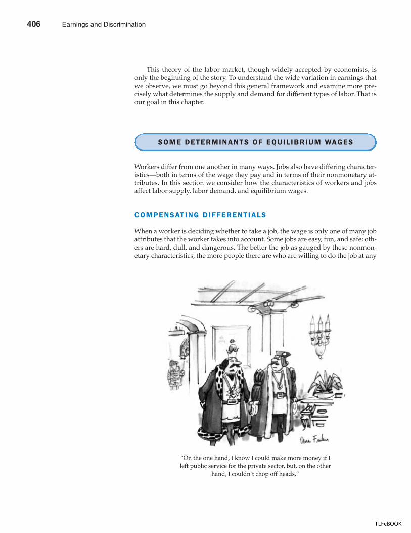
418 PART SIX THE ECONOMICS OF LABOR MARKETS
This theory of the labor market, though widely accepted by economists, isonly the beginning of the story. To understand the wide variation in earnings thatwe observe, we must go beyond this general framework and examine more pre-cisely what determines the supply and demand for different types of labor. That isour goal in this chapter.
SOME DETERMINANTS OF EQUIL IBRIUM WAGES
Workers differ from one another in many ways. Jobs also have differing character-istics—both in terms of the wage they pay and in terms of their nonmonetary at-tributes. In this section we consider how the characteristics of workers and jobsaffect labor supply, labor demand, and equilibrium wages.
COMPENSATING DIFFERENTIALS
When a worker is deciding whether to take a job, the wage is only one of many jobattributes that the worker takes into account. Some jobs are easy, fun, and safe; oth-ers are hard, dull, and dangerous. The better the job as gauged by these nonmon-etary characteristics, the more people there are who are willing to do the job at any
“On the one hand, I know I could make more money if I left public service for the private sector, but, on the other
hand, I couldn’t chop off heads.”
406 Earnings and Discrimination
TLFeBOOK
CHAPTER 19 EARNINGS AND DISCRIMINATION 419
given wage. In other words, the supply of labor for easy, fun, and safe jobs isgreater than the supply of labor for hard, dull, and dangerous jobs. As a result,“good” jobs will tend to have lower equilibrium wages than “bad” jobs.
For example, imagine you are looking for a summer job in the local beachcommunity. Two kinds of jobs are available. You can take a job as a beach-badgechecker, or you can take a job as a garbage collector. The beach-badge checkerstake leisurely strolls along the beach during the day and check to make sure thetourists have bought the required beach permits. The garbage collectors wake upbefore dawn to drive dirty, noisy trucks around town to pick up garbage. Whichjob would you want? Most people would prefer the beach job if the wages werethe same. To induce people to become garbage collectors, the town has to offerhigher wages to garbage collectors than to beach-badge checkers.
Economists use the term compensating differential to refer to a difference inwages that arises from nonmonetary characteristics of different jobs. Compensat-ing differentials are prevalent in the economy. Here are some examples:
� Coal miners are paid more than other workers with similar levels ofeducation. Their higher wage compensates them for the dirty and dangerousnature of coal mining, as well as the long-term health problems that coalminers experience.
� Workers who work the night shift at factories are paid more than similarworkers who work the day shift. The higher wage compensates them forhaving to work at night and sleep during the day, a lifestyle that most peoplefind undesirable.
� Professors are paid less than lawyers and doctors, who have similar amountsof education. Professors’ lower wages compensate them for the greatintellectual and personal satisfaction that their jobs offer. (Indeed, teachingeconomics is so much fun that it is surprising that economics professors getpaid anything at all!)
HUMAN CAPITAL
As we discussed in the previous chapter, the word capital usually refers to the econ-omy’s stock of equipment and structures. The capital stock includes the farmer’stractor, the manufacturer’s factory, and the teacher’s blackboard. The essence of cap-ital is that it is a factor of production that itself has been produced.
There is another type of capital that, while less tangible than physical capital,is just as important to the economy’s production. Human capital is the accumula-tion of investments in people. The most important type of human capital is educa-tion. Like all forms of capital, education represents an expenditure of resources atone point in time to raise productivity in the future. But, unlike an investment inother forms of capital, an investment in education is tied to a specific person, andthis linkage is what makes it human capital.
Not surprisingly, workers with more human capital on average earn morethan those with less human capital. College graduates in the United States, for ex-ample, earn about twice as much as those workers who end their education with ahigh school diploma. This large difference has been documented in many coun-tries around the world. It tends to be even larger in less developed countries,where educated workers are in scarce supply.
compensat ing d i f fe rent ia la difference in wages that arisesto offset the nonmonetarycharacteristics of different jobs
human cap i ta lthe accumulation of investments inpeople, such as education and on-the-job training
Earnings and Discrimination 407
TLFeBOOK
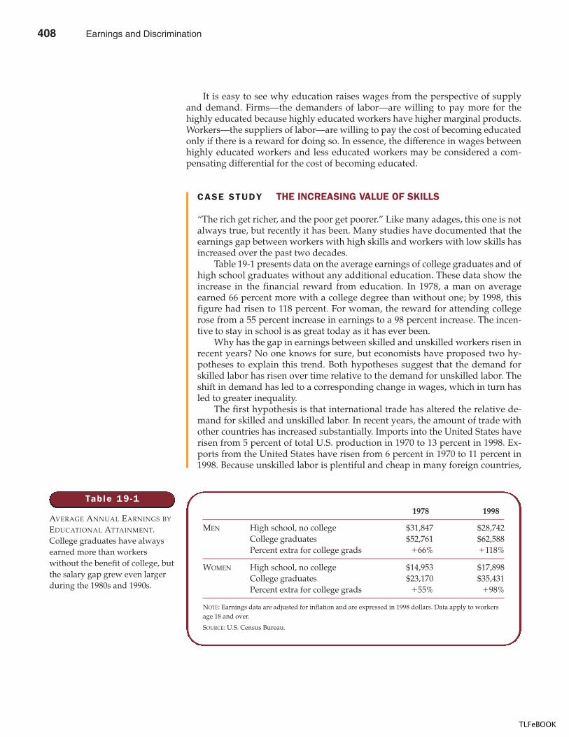
420 PART SIX THE ECONOMICS OF LABOR MARKETS
CASE STUDY THE INCREASING VALUE OF SKILLS
“The rich get richer, and the poor get poorer.” Like many adages, this one is notalways true, but recently it has been. Many studies have documented that theearnings gap between workers with high skills and workers with low skills hasincreased over the past two decades.
Table 19-1 presents data on the average earnings of college graduates and ofhigh school graduates without any additional education. These data show theincrease in the financial reward from education. In 1978, a man on averageearned 66 percent more with a college degree than without one; by 1998, thisfigure had risen to 118 percent. For woman, the reward for attending collegerose from a 55 percent increase in earnings to a 98 percent increase. The incen-tive to stay in school is as great today as it has ever been.
Why has the gap in earnings between skilled and unskilled workers risen inrecent years? No one knows for sure, but economists have proposed two hy-potheses to explain this trend. Both hypotheses suggest that the demand forskilled labor has risen over time relative to the demand for unskilled labor. Theshift in demand has led to a corresponding change in wages, which in turn hasled to greater inequality.
The first hypothesis is that international trade has altered the relative de-mand for skilled and unskilled labor. In recent years, the amount of trade withother countries has increased substantially. Imports into the United States haverisen from 5 percent of total U.S. production in 1970 to 13 percent in 1998. Ex-ports from the United States have risen from 6 percent in 1970 to 11 percent in1998. Because unskilled labor is plentiful and cheap in many foreign countries,
It is easy to see why education raises wages from the perspective of supplyand demand. Firms—the demanders of labor—are willing to pay more for thehighly educated because highly educated workers have higher marginal products.Workers—the suppliers of labor—are willing to pay the cost of becoming educatedonly if there is a reward for doing so. In essence, the difference in wages betweenhighly educated workers and less educated workers may be considered a com-pensating differential for the cost of becoming educated.
Table 19 -1
AVERAGE ANNUAL EARNINGS BY
EDUCATIONAL ATTAINMENT.College graduates have alwaysearned more than workerswithout the benefit of college, butthe salary gap grew even largerduring the 1980s and 1990s.
1978 1998
MEN High school, no college $31,847 $28,742College graduates $52,761 $62,588Percent extra for college grads �66% �118%
WOMEN High school, no college $14,953 $17,898College graduates $23,170 $35,431Percent extra for college grads �55% �98%
NOTE: Earnings data are adjusted for inflation and are expressed in 1998 dollars. Data apply to workersage 18 and over.
SOURCE: U.S. Census Bureau.
408 Earnings and Discrimination
TLFeBOOK
CHAPTER 19 EARNINGS AND DISCRIMINATION 421
the United States tends to import goods produced with unskilled labor and ex-port goods produced with skilled labor. Thus, when international trade ex-pands, the domestic demand for skilled labor rises, and the domestic demandfor unskilled labor falls.
The second hypothesis is that changes in technology have altered the rela-tive demand for skilled and unskilled labor. Consider, for instance, the intro-duction of computers. Computers raise the demand for skilled workers whocan use the new machines and reduce the demand for the unskilled workerswhose jobs are replaced by the computers. For example, many companies nowrely more on computer databases, and less on filing cabinets, to keep businessrecords. This change raises the demand for computer programmers and reducesthe demand for filing clerks. Thus, as more firms begin to use computers, thedemand for skilled labor rises, and the demand for unskilled labor falls.
Economists have found it difficult to gauge the validity of these two hy-potheses. It is possible, of course, that both are true: Increasing internationaltrade and technological change may share responsibility for the increasing in-equality we have observed in recent decades.
ABIL ITY, EFFORT, AND CHANCE
Why do major league baseball players get paid more than minor league players?Certainly, the higher wage is not a compensating differential. Playing in the majorleagues is not a less pleasant task than playing in the minor leagues; in fact, the op-posite is true. The major leagues do not require more years of schooling or moreexperience. To a large extent, players in the major leagues earn more just becausethey have greater natural ability.
Natural ability is important for workers in all occupations. Because of hered-ity and upbringing, people differ in their physical and mental attributes. Somepeople are strong, others weak. Some people are smart, others less so. Some peo-ple are outgoing, others awkward in social situations. These and many other per-sonal characteristics determine how productive workers are and, therefore, play arole in determining the wages they earn.
Closely related to ability is effort. Some people work hard; others are lazy. Weshould not be surprised to find that those who work hard are more productive andearn higher wages. To some extent, firms reward workers directly by paying peo-ple on the basis of what they produce. Salespeople, for instance, are often paid asa percentage of the sales they make. At other times, hard work is rewarded less di-rectly in the form of a higher annual salary or a bonus.
Chance also plays a role in determining wages. If a person attended a tradeschool to learn how to repair televisions with vacuum tubes and then found thisskill made obsolete by the invention of solid-state electronics, he or she would endup earning a low wage compared to others with similar years of training. The lowwage of this worker is due to chance—a phenomenon that economists recognizebut do not shed much light on.
How important are ability, effort, and chance in determining wages? It is hardto say, because ability, effort, and chance are hard to measure. But indirect evi-dence suggests that they are very important. When labor economists study wages,they relate a worker’s wage to those variables that can be measured—years ofschooling, years of experience, age, and job characteristics. Although all of these
Earnings and Discrimination 409
TLFeBOOK
422 PART SIX THE ECONOMICS OF LABOR MARKETS
CASE STUDY THE BENEFITS OF BEAUTY
People differ in many ways. One difference is in how attractive they are. The ac-tor Mel Gibson, for instance, is a handsome man. In part for this reason, hismovies attract large audiences. Not surprisingly, the large audiences mean alarge income for Mr. Gibson.
How prevalent are the economic benefits of beauty? Labor economists DanielHamermesh and Jeff Biddle tried to answer this question in a study published inthe December 1994 issue of the American Economic Review. Hamermesh and Bid-dle examined data from surveys of individuals in the United States and Canada.The interviewers who conducted the survey were asked to rate each respondent’sphysical appearance. Hamermesh and Biddle then examined how much thewages of the respondents depended on the standard determinants—education,experience, and so on—and how much they depended on physical appearance.
Hamermesh and Biddle found that beauty pays. People who are deemed tobe more attractive than average earn 5 percent more than people of averagelooks. People of average looks earn 5 to 10 percent more than people consideredless attractive than average. Similar results were found for men and women.
What explains these differences in wages? There are several ways to inter-pret the “beauty premium.”
One interpretation is that good looks are themselves a type of innate abilitydetermining productivity and wages. Some people are born with the attributesof a movie star; other people are not. Good looks are useful in any job in whichworkers present themselves to the public—such as acting, sales, and waiting ontables. In this case, an attractive worker is more valuable to the firm than an un-attractive worker. The firm’s willingness to pay more to attractive workers re-flects its customers’ preferences.
A second interpretation is that reported beauty is an indirect measure ofother types of ability. How attractive a person appears depends on more thanjust heredity. It also depends on dress, hairstyle, personal demeanor, and otherattributes that a person can control. Perhaps a person who successfully projectsan attractive image in a survey interview is more likely to be an intelligent per-son who succeeds at other tasks as well.
A third interpretation is that the beauty premium is a type of discrimina-tion, a topic to which we return later.
measured variables affect a worker’s wage as theory predicts, they account for lessthan half of the variation in wages in our economy. Because so much of the varia-tion in wages is left unexplained, omitted variables, including ability, effort, andchance, must play an important role.
GOOD LOOKS PAY.
AN ALTERNATIVE VIEW OF EDUCATION: S IGNALING
Earlier we discussed the human-capital view of education, according to whichschooling raises workers’ wages because it makes them more productive. Al-though this view is widely accepted, some economists have proposed an alterna-tive theory, which emphasizes that firms use educational attainment as a way ofsorting between high-ability and low-ability workers. According to this alternative
410 Earnings and Discrimination
TLFeBOOK
CHAPTER 19 EARNINGS AND DISCRIMINATION 423
CASE STUDY HUMAN CAPITAL, NATURAL ABILITY, ANDCOMPULSORY SCHOOL ATTENDANCE
Does attending school increase wages because it increases productivity, or doesit only appear to increase productivity because high-ability people are morelikely to stay in school? This question is important both for judging the varioustheories of education and for evaluating alternative education policies.
If economists could conduct controlled experiments like laboratory scien-tists, it would be easy to answer this question. We could choose some experi-mental subjects from the school-age population and then randomly divide theminto various groups. For each group we could require a different amount ofschool attendance. By comparing the difference in the educational attainmentand the difference in subsequent wages of the various groups, we could seewhether education does in fact increase productivity. Because the groups wouldbe chosen randomly, we could be sure that the difference in wages was not at-tributable to a difference in natural ability.
Although conducting such an experiment might seem difficult, the laws ofthe United States inadvertently provide a natural experiment that is quite simi-lar. All students in the United States are required by law to attend school, butthe laws vary from state to state. Some states allow students to drop out at age
view, when people earn a college degree, for instance, they do not become moreproductive, but they do signal their high ability to prospective employers. Becauseit is easier for high-ability people to earn a college degree than it is for low-abilitypeople, more high-ability people get college degrees. As a result, it is rational forfirms to interpret a college degree as a signal of ability.
The signaling theory of education is similar to the signaling theory of adver-tising discussed in Chapter 17. In the signaling theory of advertising, the adver-tisement itself contains no real information, but the firm signals the quality of itsproduct to consumers by its willingness to spend money on advertising. In thesignaling theory of education, schooling has no real productivity benefit, but theworker signals his innate productivity to employers by his willingness to spendyears at school. In both cases, an action is being taken not for its intrinsic benefitbut because the willingness to take that action conveys private information tosomeone observing it.
Thus, we now have two views of education: the human-capital theory and thesignaling theory. Both views can explain why more educated workers tend to earnmore than less educated workers. According to the human-capital view, educationmakes workers more productive; according to the signaling view, education is cor-related with natural ability. But the two views have radically different predictionsfor the effects of policies that aim to increase educational attainment. According tothe human-capital view, increasing educational levels for all workers would raiseall workers’ productivity and thereby their wages. According to the signalingview, education does not enhance productivity, so raising all workers’ educationallevels would not affect wages.
Most likely, truth lies somewhere between these two extremes. The benefits toeducation are probably a combination of the productivity-enhancing effects of hu-man capital and the productivity-revealing effects of signaling. The open questionis the relative size of these two effects.
Earnings and Discrimination 411
TLFeBOOK
424 PART SIX THE ECONOMICS OF LABOR MARKETS
16, while others require attendance until age 17 or 18. Moreover, the laws havechanged over time. Between 1970 and 1980, for instance, Wyoming reduced theschool-attendance age from 17 to 16, while Washington raised it from 16 to 18.This variation across states and over time provides data with which to study theeffects of compulsory school attendance.
Even within a state, school-attendance laws have different effects on differ-ent people. Students start attending school at different ages, depending on themonth of the year in which they were born. Yet all students can drop out assoon as they reach the minimum legal age; they are not required to finish outthe school year. As a result, those who start school at a relatively young age arerequired to spend more time in school than those who start school at a relativelyold age. This variation across students within a state also provides a way tostudy the effects of compulsory attendance.
In an article published in the November 1991 issue of the Quarterly Journal ofEconomics, labor economists Joshua Angrist and Alan Krueger used this naturalexperiment to study the relationship between schooling and wages. Because theduration of each student’s compulsory schooling depends on his or her state ofresidence and month of birth, and not on natural ability, it was possible to isolatethe productivity-enhancing effect of education from the ability-signaling effect.According to Angrist and Krueger’s research, those students who were requiredto finish more school did earn significantly higher subsequent wages than thosewith lower requirements. This finding indicates that education does raise aworker’s productivity, as the human-capital theory suggests.
Although establishing the benefits of compulsory schooling is useful, it doesnot by itself tell us whether these laws are desirable. That policy judgment re-quires a more complete analysis of the costs and benefits. At the very least, wewould need to compare the benefits of schooling to the opportunity cost—thewages that the student could have earned by dropping out. In addition, requir-ing a student to stay in school may have external effects on others in society. Onthe one hand, compulsory school attendance may reduce crime rates, for youngdropouts are at high risk of engaging in criminal activity. On the other hand, stu-dents who stay in school only because they are required to do so may interferewith the learning of other students who are more committed to their educations.
THE SUPERSTAR PHENOMENON
Although most actors earn very little and often have to take jobs as waiters tosupport themselves, actor Robin Williams earned $23 million in 1997. Similarly,although most people who play football do it for free as a hobby, Brett Favre earned$6.75 million as a pro quarterback. Robin Williams and Brett Favre are superstars intheir fields, and their great public appeal is reflected in astronomical incomes.
Why do Robin Williams and Brett Favre earn so much? It is not surprising thatthere are differences in incomes within occupations. Good carpenters earn morethan mediocre carpenters, and good plumbers earn more than mediocre plumbers.People vary in ability and effort, and these differences lead to differences in in-come. Yet the best carpenters and plumbers do not earn the many millions that arecommon among the best actors and athletes. What explains the difference?
To understand the tremendous incomes of Robin Williams and Brett Favre, wemust examine the special features of the markets in which they sell their services.Superstars arise in markets that have two characteristics:
412 Earnings and Discrimination
TLFeBOOK
CHAPTER 19 EARNINGS AND DISCRIMINATION 425
� Every customer in the market wants to enjoy the good supplied by the bestproducer.
� The good is produced with a technology that makes it possible for the bestproducer to supply every customer at low cost.
If Robin Williams is the funniest actor around, then everyone will want to see hisnext movie; seeing twice as many movies by an actor half as funny is not a goodsubstitute. Moreover, it is possible for everyone to enjoy the comedy of RobinWilliams. Because it is easy to make multiple copies of a film, Robin Williams canprovide his service to millions of people simultaneously. Similarly, because foot-ball games are broadcast on television, millions of fans can enjoy the extraordinaryathletic skills of Brett Favre.
We can now see why there are no superstar carpenters and plumbers. Otherthings equal, everyone prefers to employ the best carpenter, but a carpenter, unlikea movie actor, can provide his services to only a limited number of customers. Al-though the best carpenter will be able to command a somewhat higher wage thanthe average carpenter, the average carpenter will still be able to earn a good living.
ABOVE-EQUIL IBRIUM WAGES: MINIMUM-WAGE LAWS, UNIONS, AND EFFICIENCY WAGES
Most analyses of wage differences among workers are based on the equilibriummodel of the labor market—that is, wages are assumed to adjust to balance laborsupply and labor demand. But this assumption does not always apply. For someworkers, wages are set above the level that brings supply and demand into equi-librium. Let’s consider three reasons why this might be so.
One reason for above-equilibrium wages is minimum-wage laws, as we firstsaw in Chapter 6. Most workers in the economy are not affected by these laws be-cause their equilibrium wages are well above the legal minimum. But for someworkers, especially the least skilled and experienced, minimum-wage laws raisewages above the level they would earn in an unregulated labor market.
A second reason that wages might rise above their equilibrium level is themarket power of labor unions. A union is a worker association that bargains withemployers over wages and working conditions. Unions often raise wages abovethe level that would prevail without a union, perhaps because they can threaten towithhold labor from the firm by calling a strike. Studies suggest that union work-ers earn about 10 to 20 percent more than similar nonunion workers.
A third reason for above-equilibrium wages is suggested by the theory of effi-ciency wages. This theory holds that a firm can find it profitable to pay high wagesbecause doing so increases the productivity of its workers. In particular, highwages may reduce worker turnover, increase worker effort, and raise the qualityof workers who apply for jobs at the firm. If this theory is correct, then some firmsmay choose to pay their workers more than they would normally earn.
Above-equilibrium wages, whether caused by minimum-wage laws, unions,or efficiency wages, have similar effects on the labor market. In particular, pushinga wage above the equilibrium level raises the quantity of labor supplied and re-duces the quantity of labor demanded. The result is a surplus of labor, or unem-ployment. The study of unemployment and the public policies aimed to deal withit is usually considered a topic within macroeconomics, so it goes beyond thescope of this chapter. But it would be a mistake to ignore these issues completely
uniona worker association that bargainswith employers over wages andworking conditions
st r ikethe organized withdrawal of laborfrom a firm by a union
ef f ic iency wagesabove-equilibrium wages paid byfirms in order to increase workerproductivity
Earnings and Discrimination 413
TLFeBOOK
426 PART SIX THE ECONOMICS OF LABOR MARKETS
when analyzing earnings. Although most wage differences can be understoodwhile maintaining the assumption of equilibrium in the labor market, above-equilibrium wages play a role in some cases.
QUICK QUIZ: Define compensating differential and give an example.� Give two reasons why more educated workers earn more than less educated workers.
THE ECONOMICS OF DISCRIMINATION
Another source of differences in wages is discrimination. Discrimination occurswhen the marketplace offers different opportunities to similar individuals whodiffer only by race, ethnic group, sex, age, or other personal characteristics. Dis-crimination reflects some people’s prejudice against certain groups in society. Al-though discrimination is an emotionally charged topic that often generates heateddebate, economists try to study the topic objectively in order to separate mythfrom reality.
MEASURING LABOR-MARKET DISCRIMINATION
How much does discrimination in labor markets affect the earnings of differentgroups of workers? This question is important, but answering it is not easy.
It might seem natural to gauge the amount of discrimination in labor marketsby looking at the average wages of different groups. For instance, in recent yearsthe wage of the average black worker in the United States has been about 20 per-cent less than the wage of the average white worker. The wage of the average fe-male worker has been about 30 percent less than the wage of the average maleworker. These wage differentials are sometimes presented in political debate as ev-idence that many employers discriminate against blacks and women.
Yet there is an obvious problem with this approach. Even in a labor market freeof discrimination, different people have different wages. People differ in theamount of human capital they have and in the kinds of work they are able and will-ing to do. The wage differences we observe in the economy are, to a large extent, at-tributable to the determinants of equilibrium wages we discussed in the precedingsection. Simply observing differences in wages among broad groups—whites andblacks, men and women—says little about the prevalence of discrimination.
Consider, for example, the role of human capital. About 80 percent of whitemale workers have a high school diploma, and 25 percent have a college degree.By contrast, only 67 percent of black male workers have a high school diploma,and only 12 percent have a college degree. Thus, at least some of the difference be-tween the wages of whites and the wages of blacks can be traced to differences ineducational attainment. Similarly, among white workers, 25 percent of men have acollege degree, whereas only 19 percent of women have a college degree, indicat-ing that some of the difference between the wages of men and women is attribut-able to educational attainment.
discr iminat ionthe offering of different opportunitiesto similar individuals who differ onlyby race, ethnic group, sex, age, orother personal characteristics
414 Earnings and Discrimination
TLFeBOOK
CHAPTER 19 EARNINGS AND DISCRIMINATION 427
In fact, human capital is probably even more important in explaining wagedifferentials than the foregoing numbers suggest. For many years, public schoolsin predominantly black areas have been of lower quality—as measured by expen-diture, class size, and so on—than public schools in predominantly white areas.Similarly, for many years, schools directed girls away from science and mathcourses, even though these subjects may have had greater value in the market-place than some of the alternatives. If we could measure the quality as well as thequantity of education, the differences in human capital among these groups wouldseem even larger.
Human capital acquired in the form of job experience can also help explainwage differences. In particular, women tend to have less job experience on averagethan men. One reason is that female labor-force participation has increased over thepast several decades. Because of this historic change, the average female worker to-day is younger than the average male worker. In addition, women are more likelyto interrupt their careers to raise children. For both reasons, the experience of theaverage female worker is less than the experience of the average male worker.
Yet another source of wage differences is compensating differentials. Some an-alysts have suggested that women take more pleasant jobs on average than menand that this fact explains some of the earnings differential between men andwomen. For example, women are more likely to be secretaries, and men are morelikely to be truck drivers. The relative wages of secretaries and truck drivers de-pend in part on the working conditions of each job. Because these nonmonetary as-pects are hard to measure, it is difficult to gauge the practical importance ofcompensating differentials in explaining the wage differences that we observe.
In the end, the study of wage differences among groups does not establish anyclear conclusion about the prevalence of discrimination in U.S. labor markets.Most economists believe that some of the observed wage differentials are attribut-able to discrimination, but there is no consensus about how much. The only con-clusion about which economists are in consensus is a negative one: Because thedifferences in average wages among groups in part reflect differences in human capital andjob characteristics, they do not by themselves say anything about how much discriminationthere is in the labor market.
Of course, differences in human capital among groups of workers may them-selves reflect discrimination. The inferior schools historically available to blackstudents, for instance, may be traced to prejudice on the part of city councils andschool boards. But this kind of discrimination occurs long before the worker entersthe labor market. In this case, the disease is political, even if the symptom iseconomic.
DISCRIMINATION BY EMPLOYERS
Let’s now turn from measurement to the economic forces that lie behind discrimi-nation in labor markets. If one group in society receives a lower wage than anothergroup, even after controlling for human capital and job characteristics, who is toblame for this differential?
The answer is not obvious. It might seem natural to blame employers for dis-criminatory wage differences. After all, employers make the hiring decisions that de-termine labor demand and wages. If some groups of workers earn lower wages thanthey should, then it seems that employers are responsible. Yet many economists are
Earnings and Discrimination 415
TLFeBOOK
428 PART SIX THE ECONOMICS OF LABOR MARKETS
CASE STUDY SEGREGATED STREETCARS ANDTHE PROFIT MOTIVE
In the early twentieth century, streetcars in many southern cities were segre-gated by race. White passengers sat in the front of the streetcars, and black pas-sengers sat in the back. What do you suppose caused and maintained thisdiscriminatory practice? And how was this practice viewed by the firms thatran the streetcars?
In a 1986 article in the Journal of Economic History, economic historian Jen-nifer Roback looked at these questions. Roback found that the segregation ofraces on streetcars was the result of laws that required such segregation. Beforethese laws were passed, racial discrimination in seating was rare. It was farmore common to segregate smokers and nonsmokers.
Moreover, the firms that ran the streetcars often opposed the laws requiringracial segregation. Providing separate seating for different races raised thefirms’ costs and reduced their profit. One railroad company manager com-plained to the city council that, under the segregation laws, “the company hasto haul around a good deal of empty space.”
Here is how Roback describes the situation in one southern city:
The railroad company did not initiate the segregation policy and was not atall eager to abide by it. State legislation, public agitation, and a threat toarrest the president of the railroad were all required to induce them toseparate the races on their cars. . . . There is no indication that themanagement was motivated by belief in civil rights or racial equality. Theevidence indicates their primary motives were economic; separation was
skeptical of this easy answer. They believe that competitive, market economies pro-vide a natural antidote to employer discrimination. That antidote is called the profitmotive.
Imagine an economy in which workers are differentiated by their hair color.Blondes and brunettes have the same skills, experience, and work ethic. Yet, be-cause of discrimination, employers prefer not to hire workers with blonde hair.Thus, the demand for blondes is lower than it otherwise would be. As a result,blondes earn a lower wage than brunettes.
How long can this wage differential persist? In this economy, there is an easyway for a firm to beat out its competitors: It can hire blonde workers. By hiringblondes, a firm pays lower wages and thus has lower costs than firms that hirebrunettes. Over time, more and more “blonde” firms enter the market to take ad-vantage of this cost advantage. The existing “brunette” firms have higher costsand, therefore, begin to lose money when faced with the new competitors. Theselosses induce the brunette firms to go out of business. Eventually, the entry ofblonde firms and the exit of brunette firms cause the demand for blonde workersto rise and the demand for brunette workers to fall. This process continues untilthe wage differential disappears.
Put simply, business owners who care only about making money are at an ad-vantage when competing against those who also care about discriminating. As aresult, firms that do not discriminate tend to replace those that do. In this way,competitive markets have a natural remedy for employer discrimination.
416 Earnings and Discrimination
TLFeBOOK
CHAPTER 19 EARNINGS AND DISCRIMINATION 429
costly. . . . Officials of the company may or may not have disliked blacks,but they were not willing to forgo the profits necessary to indulge suchprejudice.
The story of southern streetcars illustrates a general lesson: Business owners areusually more interested in making profit than in discriminating against a par-ticular group. When firms engage in discriminatory practices, the ultimatesource of the discrimination often lies not with the firms themselves but else-where. In this particular case, the streetcar companies segregated whites andblacks because discriminatory laws, which the companies opposed, requiredthem to do so.
DISCRIMINATION BY CUSTOMERS AND GOVERNMENTS
Although the profit motive is a strong force acting to eliminate discriminatorywage differentials, there are limits to its corrective abilities. Here we consider twoof the most important limits: customer preferences and government policies.
To see how customer preferences for discrimination can affect wages, consideragain our imaginary economy with blondes and brunettes. Suppose that restau-rant owners discriminate against blondes when hiring waiters. As a result, blondewaiters earn lower wages than brunette waiters. In this case, a restaurant couldopen up with blonde waiters and charge lower prices. If customers only caredabout the quality and price of their meals, the discriminatory firms would be dri-ven out of business, and the wage differential would disappear.
On the other hand, it is possible that customers prefer being served by brunettewaiters. If this preference for discrimination is strong, the entry of blonde restau-rants need not succeed in eliminating the wage differential between brunettes andblondes. That is, if customers have discriminatory preferences, a competitive mar-ket is consistent with a discriminatory wage differential. An economy with suchdiscrimination would contain two types of restaurants. Blonde restaurants hireblondes, have lower costs, and charge lower prices. Brunette restaurants hirebrunettes, have higher costs, and charge higher prices. Customers who did not careabout the hair color of their waiters would be attracted to the lower prices at theblonde restaurants. Bigoted customers would go to the brunette restaurants. Theywould pay for their discriminatory preference in the form of higher prices.
Another way for discrimination to persist in competitive markets is for thegovernment to mandate discriminatory practices. If, for instance, the governmentpassed a law stating that blondes could wash dishes in restaurants but could notwork as waiters, then a wage differential could persist in a competitive market.The example of segregated streetcars in the foregoing case study is one example ofgovernment-mandated discrimination. More recently, before South Africa aban-doned its system of apartheid, blacks were prohibited from working in some jobs.Discriminatory governments pass such laws to suppress the normal equalizingforce of free and competitive markets.
To sum up: Competitive markets contain a natural remedy for employer discrimina-tion. The entry of firms that care only about profit tends to eliminate discriminatory wagedifferentials. These wage differentials persist in competitive markets only when customersare willing to pay to maintain the discriminatory practice or when the government man-dates it.
Earnings and Discrimination 417
TLFeBOOK

430 PART SIX THE ECONOMICS OF LABOR MARKETS
CASE STUDY DISCRIMINATION IN SPORTS
As we have seen, measuring discrimination is often difficult. To determinewhether one group of workers is discriminated against, a researcher must cor-rect for differences in the productivity between that group and other workers inthe economy. Yet, in most firms, it is difficult to measure a particular worker’scontribution to the production of goods and services.
One type of firm in which such corrections are easier is the sports team. Pro-fessional teams have many objective measures of productivity. In baseball, forinstance, we can measure a player’s batting average, the frequency of homeruns, the number of stolen bases, and so on.
Studies of sports teams suggest that racial discrimination is, in fact, commonand that much of the blame lies with customers. One study, published in the Jour-nal of Labor Economics in 1988, examined the salaries of basketball players. It foundthat black players earned 20 percent less than white players of comparable ability.The study also found that attendance at basketball games was larger for teams
WHY DOES THE AVERAGE FEMALE WORKER
earn less than the average maleworker? In the following article, econo-mist June O’Neill offers some answersto this question.
T h e S h r i n k i n g P a y G a p
BY JUNE ELLENOFF O’NEILL
“Fifty-nine cents,” the popular buttonsaid, a symbol of the stubborn fact thatthroughout the post–World War II period,women’s wages hovered at around 60percent of men’s, despite an increasingproportion of women working outsidethe home. This gender gap did not de-cline through the 1960s and the 1970s
despite the rise of the feminist move-ment, equal pay and employment legisla-tion, and affirmative action.
But starting in the Reagan years, thegender gap in wages began to declinedramatically. By some measures the ratioof women’s earnings to men’s rose tonearly 80 percent; and even this number,I believe, overstates the gender gap be-tween men and women with similar skillsand training. Why did this dramatic nar-rowing in relative wages happen?
The answer has less to do with poli-tics or protests than with the realities ofthe labor market. Although basic skillsare acquired in school, it is in the labormarket where specialized skills are de-veloped that bring higher wages. Duringthe three decades following World War IIwomen entered the labor market inrecord numbers. But many of the newentrants had been out of the labor forcefor considerable periods of time, raisingtheir children. These women diluted theskill level of the rapidly expanding groupof employed women. This was the mainreason why the gender gap in pay didnot narrow during the postwar years.
Today’s working women, particularlythose younger than forty, are much morenearly equal to men in work experiencethan were their mothers. Through delayedmarriage, low fertility, and an increasingtendency for mothers of young children towork, women have acquired many moreyears of continuous work experience thanwas true in the past. (Close to 60 percentof married women with children under agesix are now in the labor force; in 1960, theproportion was only 19 percent.)
And the work experience gained bythese younger women is likely to have aneven greater impact on their future earn-ings because their work experience hasbeen more correctly anticipated. Many in-vestment choices affecting careers aremade at younger ages: years of school-ing, subjects in school, other professionaltraining. In the past, women were muchless likely than men to invest in lengthytraining because they assumed theywould not be working enough years tojustify it.
In fact, the National LongitudinalSurveys found that even in the late1960s less than 30 percent of young
IN THE NEWS
Men, Women, and Wages
418 Earnings and Discrimination
TLFeBOOK
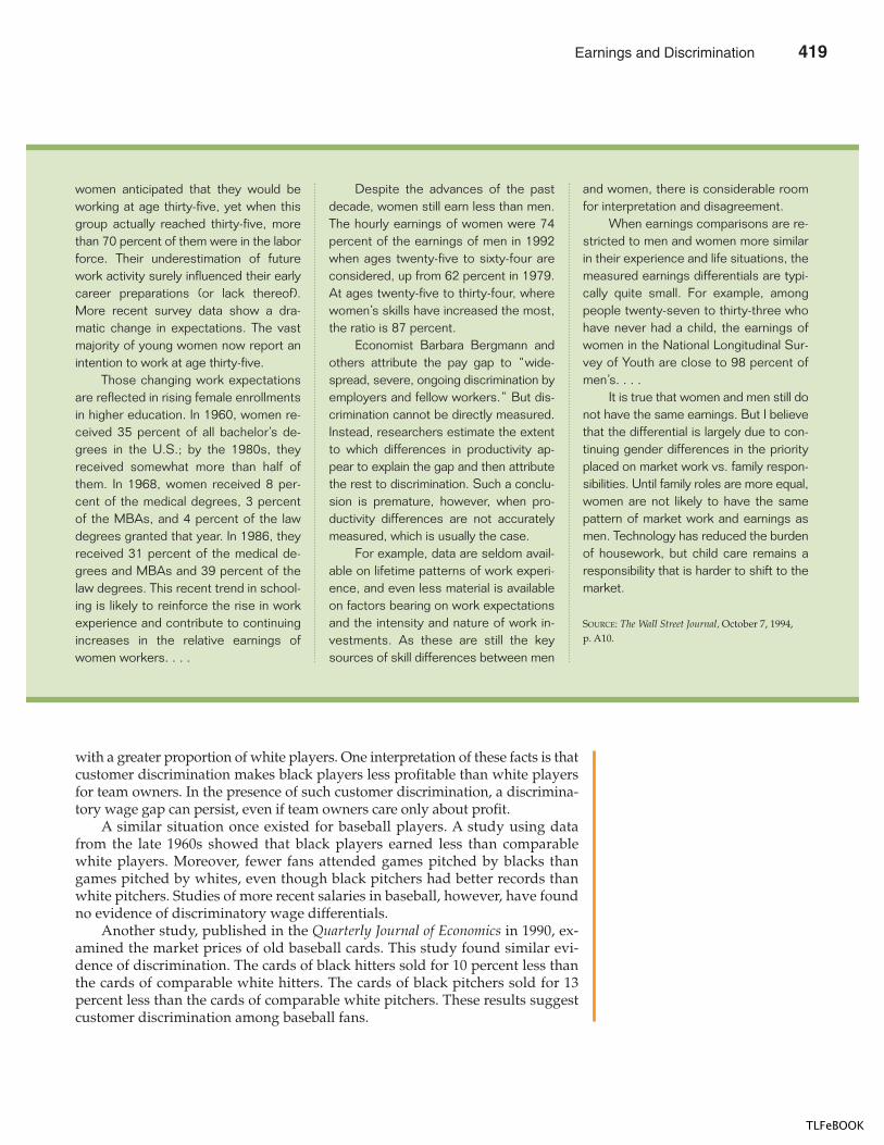
CHAPTER 19 EARNINGS AND DISCRIMINATION 431
with a greater proportion of white players. One interpretation of these facts is thatcustomer discrimination makes black players less profitable than white playersfor team owners. In the presence of such customer discrimination, a discrimina-tory wage gap can persist, even if team owners care only about profit.
A similar situation once existed for baseball players. A study using datafrom the late 1960s showed that black players earned less than comparablewhite players. Moreover, fewer fans attended games pitched by blacks thangames pitched by whites, even though black pitchers had better records thanwhite pitchers. Studies of more recent salaries in baseball, however, have foundno evidence of discriminatory wage differentials.
Another study, published in the Quarterly Journal of Economics in 1990, ex-amined the market prices of old baseball cards. This study found similar evi-dence of discrimination. The cards of black hitters sold for 10 percent less thanthe cards of comparable white hitters. The cards of black pitchers sold for 13percent less than the cards of comparable white pitchers. These results suggestcustomer discrimination among baseball fans.
women anticipated that they would beworking at age thirty-five, yet when thisgroup actually reached thirty-five, morethan 70 percent of them were in the laborforce. Their underestimation of futurework activity surely influenced their earlycareer preparations (or lack thereof).More recent survey data show a dra-matic change in expectations. The vastmajority of young women now report anintention to work at age thirty-five.
Those changing work expectationsare reflected in rising female enrollmentsin higher education. In 1960, women re-ceived 35 percent of all bachelor’s de-grees in the U.S.; by the 1980s, theyreceived somewhat more than half ofthem. In 1968, women received 8 per-cent of the medical degrees, 3 percentof the MBAs, and 4 percent of the lawdegrees granted that year. In 1986, theyreceived 31 percent of the medical de-grees and MBAs and 39 percent of thelaw degrees. This recent trend in school-ing is likely to reinforce the rise in workexperience and contribute to continuingincreases in the relative earnings ofwomen workers. . . .
Despite the advances of the pastdecade, women still earn less than men.The hourly earnings of women were 74percent of the earnings of men in 1992when ages twenty-five to sixty-four areconsidered, up from 62 percent in 1979.At ages twenty-five to thirty-four, wherewomen’s skills have increased the most,the ratio is 87 percent.
Economist Barbara Bergmann andothers attribute the pay gap to “wide-spread, severe, ongoing discrimination byemployers and fellow workers.” But dis-crimination cannot be directly measured.Instead, researchers estimate the extentto which differences in productivity ap-pear to explain the gap and then attributethe rest to discrimination. Such a conclu-sion is premature, however, when pro-ductivity differences are not accuratelymeasured, which is usually the case.
For example, data are seldom avail-able on lifetime patterns of work experi-ence, and even less material is availableon factors bearing on work expectationsand the intensity and nature of work in-vestments. As these are still the keysources of skill differences between men
and women, there is considerable roomfor interpretation and disagreement.
When earnings comparisons are re-stricted to men and women more similarin their experience and life situations, themeasured earnings differentials are typi-cally quite small. For example, amongpeople twenty-seven to thirty-three whohave never had a child, the earnings ofwomen in the National Longitudinal Sur-vey of Youth are close to 98 percent ofmen’s. . . .
It is true that women and men still donot have the same earnings. But I believethat the differential is largely due to con-tinuing gender differences in the priorityplaced on market work vs. family respon-sibilities. Until family roles are more equal,women are not likely to have the samepattern of market work and earnings asmen. Technology has reduced the burdenof housework, but child care remains aresponsibility that is harder to shift to themarket.
SOURCE: The Wall Street Journal, October 7, 1994,p. A10.
Earnings and Discrimination 419
TLFeBOOK
432 PART SIX THE ECONOMICS OF LABOR MARKETS
THE DEBATE OVER COMPARABLE WORTH
Should engineers get paid more than librarians? This question is at the heart of thedebate over comparable worth, a doctrine whereby jobs deemed comparable shouldbe paid the same wage.
Advocates of comparable worth point out that traditionally male occupationshave higher wages than traditionally female occupations. They believe that these oc-cupational differences are discriminatory against women. Even if women were paidthe same as men for the same type of work, the gender gap in wages would persistuntil comparable occupations were paid similar wages. Comparable-worth advo-cates want jobs rated according to a set of impartial criteria—education, experience,responsibility, working conditions, and so on. Under this system, comparably ratedjobs would pay the same wage. A librarian with a master’s degree, ten years of ex-perience, and a 40-hour workweek, for instance, would be paid the same as an engi-neer with a master’s degree, ten years of experience, and a 40-hour workweek.
Most economists are critical of comparable-worth proposals. They argue thata competitive market is the best mechanism for setting wages. It would be nearlyimpossible, they claim, to measure all of the factors that are relevant for determin-ing the right wage for any job. Moreover, the fact that traditionally female occupa-tions pay less than traditionally male occupations is not by itself evidence ofdiscrimination. Women have in the past spent more time than men raising chil-dren. Women are, therefore, more likely to choose occupations that offer flexiblehours and other working conditions compatible with child-rearing. To some ex-tent, the gender gap in wages is a compensating differential.
Economists also point out that comparable-worth proposals would have animportant unintended side effect. Comparable-worth advocates want the wages intraditionally female occupations to be raised by legal decree. Such a policy wouldhave many of the effects of a minimum wage, which we first discussed in Chapter6. In particular, when the wage is forced to rise above the equilibrium level, thequantity of labor supplied to these occupations would rise, and the quantity de-manded would fall. The result would be higher unemployment in traditionally fe-male occupations. In this way, a comparable-worth law could adversely affectsome members of groups that the policy is aimed at helping.
QUICK QUIZ: Why is it hard to establish whether a group of workers is being discriminated against? � Explain how profit-maximizing firms tend to eliminate discriminatory wage differentials. � How might a discriminatory wage differential persist?
CONCLUSION
In competitive markets, workers earn a wage equal to the value of their marginalcontribution to the production of goods and services. There are, however, manythings that affect the value of the marginal product. Firms pay more for workerswho are more talented, more diligent, more experienced, and more educated be-cause these workers are more productive. Firms pay less to those workers againstwhom customers discriminate because these workers contribute less to revenue.
comparab le wor tha doctrine according to which jobsdeemed comparable should be paidthe same wage
420 Earnings and Discrimination
TLFeBOOK
CHAPTER 19 EARNINGS AND DISCRIMINATION 433
The theory of the labor market we have developed in the last two chapters ex-plains why some workers earn higher wages than other workers. The theory doesnot say that the resulting distribution of income is equal, fair, or desirable in anyway. That is the topic we take up in Chapter 20.
OVER THE PAST SEVERAL YEARS, THE IDEA OF
comparable worth—sometimes calledpay equity—has made a comebackamong some political leaders.
L a b o r a n d W o m e n P u s h f o r E q u a lP a y f o r E q u i v a l e n t W o r k
BY MARY LEONARD
WASHINGTON—Nobody says men andwomen shouldn’t get equal pay for doingthe same job. But what’s brewing now isa big push nationally by the president,organized labor, and women’s rightsgroups to level the gender playing fieldon wages for different but equivalentwork.
In a strategy session today, SenatorTom Harkin, an Iowa Democrat who hasbeen the lonely champion for pay-equitylegislation since 1996, will meet with JohnPodesta, the president’s chief of staff,and other officials on ways the WhiteHouse can boost his bill this year. Yester-day, the AFL-CIO launched a nationwidecampaign to pass comparable-worth billsin 24 states, including Massachusetts.
What’s going on here? Trying to de-termine comparable salaries for jobs tra-ditionally held by men and women is anold idea, discredited by some economistsas unwieldy, if not downright dumb. Theywonder who can and will decide the eco-nomic value of a riveter versus a nurse,the comparable pay for a probation offi-cer and a librarian, the equivalent pay foran auto mechanic and a secretary.
Many see pay equity, even if it is dif-ficult to enforce, as the only remedy forwage discrimination, a problem that per-sists for women, even as they haveearned advanced degrees, climbed thecorporate ladder, and plopped their chil-dren in day care while pursuing full-timejobs in large numbers. . . .
“For too long, working women havebeen seething while politicians have re-mained silent,” said Karen Nussbaum,director of the AFL-CIO’s WorkingWomen’s department. “Pay equity canright a long-standing wrong.” . . .
Diana Furchtgott-Roth, a resident fel-low at the American Enterprise Institute,says there are plenty of reasons why menand women earn different wages—senior-ity, job risk, and market demand for cer-tain skills—that have nothing to do withdiscrimination and would not be erased by“cockeyed” pay-equity laws. She saidwhen you compare men and women withthe same qualifications doing the samejobs, women earn 95 percent of men’ssalaries.
“Comparable worth is certainly mak-ing a comeback,” Furchtgott-Roth said,“and I believe it’s because feminists whosupported Clinton through the Lewinskymess are demanding a political payoff. Idon’t see any Republican support forthese proposals.”
SOURCE: The Boston Globe, February 25, 1999, pp.A1, A22.
IN THE NEWS
The Recent Push forComparable Worth
� Workers earn different wages for many reasons. Tosome extent, wage differentials compensate workers forjob attributes. Other things equal, workers in hard,unpleasant jobs get paid more than workers in easy,pleasant jobs.
� Workers with more human capital get paid more thanworkers with less human capital. The return to
accumulating human capital is high and has increasedover the past decade.
� Although years of education, experience, and jobcharacteristics affect earnings as theory predicts,there is much variation in earnings that cannotbe explained by things that economists canmeasure. The unexplained variation in earnings is
Summar y
Earnings and Discrimination 421
TLFeBOOK
434 PART SIX THE ECONOMICS OF LABOR MARKETS
largely attributable to natural ability, effort, and chance.
� Some economists have suggested that more educatedworkers earn higher wages not because education raisesproductivity but because workers with high naturalability use education as a way to signal their high abilityto employers. If this signaling theory were correct, thenincreasing the educational attainment of all workerswould not raise the overall level of wages.
� Wages are sometimes pushed above the level that bringssupply and demand into balance. Three reason forabove-equilibrium wages are minimum-wage laws,unions, and efficiency wages.
� Some differences in earnings are attributable todiscrimination on the basis of race, sex, or other factors.
Measuring the amount of discrimination is difficult,however, because one must correct for differences inhuman capital and job characteristics.
� Competitive markets tend to limit the impact ofdiscrimination on wages. If the wages of a group ofworkers are lower than those of another group forreasons not related to marginal productivity, thennondiscriminatory firms will be more profitable thandiscriminatory firms. Profit-maximizing behavior,therefore, can act to reduce discriminatory wagedifferentials. Discrimination can persist in competitivemarkets if customers are willing to pay more todiscriminatory firms or if the government passes lawsrequiring firms to discriminate.
compensating differential, p. 419human capital, p. 419union, p. 425
strike, p. 425efficiency wages, p. 425discrimination, p. 426
comparable worth, p. 432
Key Concepts
1. Why do coal miners get paid more than other workerswith similar amounts of education?
2. In what sense is education a type of capital?
3. How might education raise a worker’s wage withoutraising the worker’s productivity?
4. What conditions lead to economic superstars? Would youexpect to see superstars in dentistry? In music? Explain.
5. Give three reasons why a worker’s wage might beabove the level that balances supply and demand.
6. What difficulties arise in deciding whether a groupof workers has a lower wage because of discrimination?
7. Do the forces of economic competition tend toexacerbate or ameliorate discrimination on the basis ofrace?
8. Give an example of how discrimination might persist ina competitive market.
Quest ions fo r Rev iew
1. College students sometimes work as summer interns forprivate firms or the government. Many of thesepositions pay little or nothing.a. What is the opportunity cost of taking such a job?b. Explain why students are willing to take these jobs.c. If you were to compare the earnings later in life of
workers who had worked as interns and those who
had taken summer jobs that paid more, what wouldyou expect to find?
2. As explained in Chapter 6, a minimum-wage lawdistorts the market for low-wage labor. To reduce thisdistortion, some economists advocate a two-tieredminimum-wage system, with a regular minimum wagefor adult workers and a lower, “sub-minimum” wage
Prob lems and App l icat ions
422 Earnings and Discrimination
TLFeBOOK
CHAPTER 19 EARNINGS AND DISCRIMINATION 435
for teenage workers. Give two reasons why a singleminimum wage might distort the labor market forteenage workers more than it would the market foradult workers.
3. A basic finding of labor economics is that workers whohave more experience in the labor force are paid morethan workers who have less experience (holdingconstant the amount of formal education). Why mightthis be so? Some studies have also found that experienceat the same job (called “job tenure”) has an extrapositive influence on wages. Explain.
4. At some colleges and universities, economics professorsreceive higher salaries than professors in some otherfields.a. Why might this be true?b. Some other colleges and universities have a policy
of paying equal salaries to professors in all fields.At some of these schools, economics professorshave lighter teaching loads than professors in someother fields. What role do the differences inteaching loads play?
5. Sara works for Steve, whom she hates because of hissnobbish attitude. Yet when she looks for other jobs, thebest she can do is find a job paying $10,000 less than hercurrent salary. Should she take the job? Analyze Sara’ssituation from an economic point of view.
6. Imagine that someone were to offer you a choice: Youcould spend four years studying at the world’s bestuniversity, but you would have to keep your attendancethere a secret. Or you could be awarded an officialdegree from the world’s best university, but youcouldn’t actually attend. Which choice do you thinkwould enhance your future earnings more? What doesyour answer say about the debate over signaling versushuman capital in the role of education?
7. When recording devices were first invented almost 100years ago, musicians could suddenly supply their musicto large audiences at low cost. How do you suppose thisevent affected the income of the best musicians? Howdo you suppose it affected the income of averagemusicians?
8. Alan runs an economic consulting firm. He hiresprimarily female economists because, he says, “they willwork for less than comparable men because women
have fewer job options.” Is Alan’s behavior admirable ordespicable? If more employers were like Alan, whatwould happen to the wage differential between menand women?
9. A case study in this chapter described how customerdiscrimination in sports seems to have an importanteffect on players’ earnings. Note that this is possiblebecause sports fans know the players’ characteristics,including their race. Why is this knowledge importantfor the existence of discrimination? Give some specificexamples of industries where customer discrimination isand is not likely to influence wages.
10. Suppose that all young women were channeled intocareers as secretaries, nurses, and teachers; at the sametime, young men were encouraged to consider thesethree careers and many others as well.a. Draw a diagram showing the combined labor
market for secretaries, nurses, and teachers. Draw adiagram showing the combined labor market for allother fields. In which market is the wage higher?Do men or women receive higher wages onaverage?
b. Now suppose that society changed and encouragedboth young women and young men to consider awide range of careers. Over time, what effect wouldthis change have on the wages in the two marketsyou illustrated in part (a)? What effect would thechange have on the average wages of men andwomen?
11. Economist June O’Neill argues that “until family rolesare more equal, women are not likely to have the samepattern of market work and earnings as men.” Whatdoes she mean by the “pattern” of market work? Howdo these characteristics of jobs and careers affectearnings?
12. This chapter considers the economics of discriminationby employers, customers, and governments. Nowconsider discrimination by workers. Suppose that somebrunette workers did not like working with blondeworkers. Do you think this worker discrimination couldexplain lower wages for blonde workers? If such a wagedifferential existed, what would a profit-maximizingentrepreneur do? If there were many suchentrepreneurs, what would happen over time?
Earnings and Discrimination 423
TLFeBOOK

TLFeBOOK
IN THIS CHAPTERYOU WILL . . .
See how po l i t ica lph i losophers v iewthe government ’s
ro le in r ed ist r ibut ing
income
Examine the degreeof economic
inequa l i ty in oursoc iety
Cons ider someprob lems that a r ise
when measur ingeconomic inequa l i ty
Cons ider the var ious po l ic iesa imed at he lp ing
poor fami l ies escape pover ty
“The only difference between the rich and other people,” Mary Colum once said toErnest Hemingway, “is that the rich have more money.” Maybe so. But this claimleaves many questions unanswered. The gap between rich and poor is a fascinat-ing and important topic of study—for the comfortable rich, for the struggling poor,and for the aspiring and worried middle class.
From the previous two chapters you should have some understanding aboutwhy different people have different incomes. A person’s earnings depend on thesupply and demand for that person’s labor, which in turn depend on natural abil-ity, human capital, compensating differentials, discrimination, and so on. Becauselabor earnings make up about three-fourths of the total income in the U.S. econ-omy, the factors that determine wages are also largely responsible for determininghow the economy’s total income is distributed among the various members of so-ciety. In other words, they determine who is rich and who is poor.
I N C O M E I N E Q U A L I T Y
A N D P O V E R T Y
437
425
20
TLFeBOOK
438 PART SIX THE ECONOMICS OF LABOR MARKETS
In this chapter we discuss the distribution of income. As we shall see, thistopic raises some fundamental questions about the role of economic policy. One ofthe Ten Principles of Economics in Chapter 1 is that governments can sometimes im-prove market outcomes. This possibility is particularly important when consider-ing the distribution of income. The invisible hand of the marketplace acts toallocate resources efficiently, but it does not necessarily ensure that resources areallocated fairly. As a result, many economists—though not all—believe that thegovernment should redistribute income to achieve greater equality. In doing so,however, the government runs into another of the Ten Principles of Economics: Peo-ple face tradeoffs. When the government enacts policies to make the distributionof income more equitable, it distorts incentives, alters behavior, and makes the al-location of resources less efficient.
Our discussion of the distribution of income proceeds in three steps. First, weassess how much inequality there is in our society. Second, we consider some dif-ferent views about what role the government should play in altering the distribu-tion of income. Third, we discuss various public policies aimed at helping society’spoorest members.
THE MEASUREMENT OF INEQUALITY
We begin our study of the distribution of income by addressing four questions ofmeasurement:
� How much inequality is there in our society?� How many people live in poverty?
“As far as I’m concerned, they can do what they want with the minimum wage, just as long as they keep their hands off the
maximum wage.”
426 Income Inequality and Poverty
TLFeBOOK
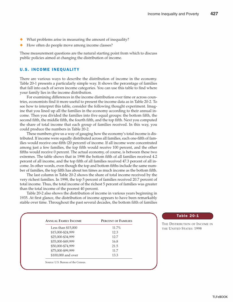
CHAPTER 20 INCOME INEQUALITY AND POVERTY 439
� What problems arise in measuring the amount of inequality?� How often do people move among income classes?
These measurement questions are the natural starting point from which to discusspublic policies aimed at changing the distribution of income.
U.S. INCOME INEQUALITY
There are various ways to describe the distribution of income in the economy.Table 20-1 presents a particularly simple way. It shows the percentage of familiesthat fall into each of seven income categories. You can use this table to find whereyour family lies in the income distribution.
For examining differences in the income distribution over time or across coun-tries, economists find it more useful to present the income data as in Table 20-2. Tosee how to interpret this table, consider the following thought experiment. Imag-ine that you lined up all the families in the economy according to their annual in-come. Then you divided the families into five equal groups: the bottom fifth, thesecond fifth, the middle fifth, the fourth fifth, and the top fifth. Next you computedthe share of total income that each group of families received. In this way, youcould produce the numbers in Table 20-2.
These numbers give us a way of gauging how the economy’s total income is dis-tributed. If income were equally distributed across all families, each one-fifth of fam-ilies would receive one-fifth (20 percent) of income. If all income were concentratedamong just a few families, the top fifth would receive 100 percent, and the otherfifths would receive 0 percent. The actual economy, of course, is between these twoextremes. The table shows that in 1998 the bottom fifth of all families received 4.2percent of all income, and the top fifth of all families received 47.3 percent of all in-come. In other words, even though the top and bottom fifths include the same num-ber of families, the top fifth has about ten times as much income as the bottom fifth.
The last column in Table 20-2 shows the share of total income received by thevery richest families. In 1998, the top 5 percent of families received 20.7 percent oftotal income. Thus, the total income of the richest 5 percent of families was greaterthan the total income of the poorest 40 percent.
Table 20-2 also shows the distribution of income in various years beginning in1935. At first glance, the distribution of income appears to have been remarkablystable over time. Throughout the past several decades, the bottom fifth of families
Table 20 -1
THE DISTRIBUTION OF INCOME IN
THE UNITED STATES: 1998
ANNUAL FAMILY INCOME PERCENT OF FAMILIES
Less than $15,000 11.7%$15,000-$24,999 12.3$25,000-$34,999 12.7$35,000-$49,999 16.8$50,000-$74,999 21.5$75,000-$99,999 11.7$100,000 and over 13.3
Source: U.S. Bureau of the Census.
Income Inequality and Poverty 427
TLFeBOOK
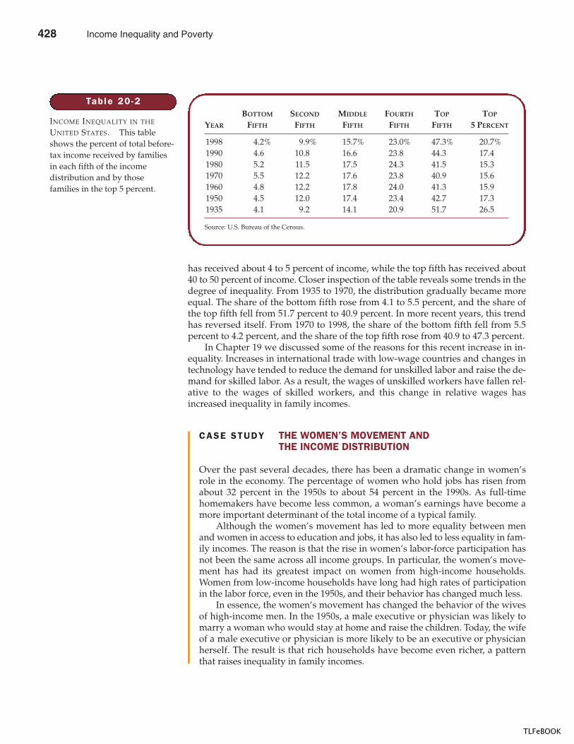
440 PART SIX THE ECONOMICS OF LABOR MARKETS
CASE STUDY THE WOMEN’S MOVEMENT ANDTHE INCOME DISTRIBUTION
Over the past several decades, there has been a dramatic change in women’srole in the economy. The percentage of women who hold jobs has risen fromabout 32 percent in the 1950s to about 54 percent in the 1990s. As full-timehomemakers have become less common, a woman’s earnings have become amore important determinant of the total income of a typical family.
Although the women’s movement has led to more equality between menand women in access to education and jobs, it has also led to less equality in fam-ily incomes. The reason is that the rise in women’s labor-force participation hasnot been the same across all income groups. In particular, the women’s move-ment has had its greatest impact on women from high-income households.Women from low-income households have long had high rates of participationin the labor force, even in the 1950s, and their behavior has changed much less.
In essence, the women’s movement has changed the behavior of the wivesof high-income men. In the 1950s, a male executive or physician was likely tomarry a woman who would stay at home and raise the children. Today, the wifeof a male executive or physician is more likely to be an executive or physicianherself. The result is that rich households have become even richer, a patternthat raises inequality in family incomes.
has received about 4 to 5 percent of income, while the top fifth has received about40 to 50 percent of income. Closer inspection of the table reveals some trends in thedegree of inequality. From 1935 to 1970, the distribution gradually became moreequal. The share of the bottom fifth rose from 4.1 to 5.5 percent, and the share ofthe top fifth fell from 51.7 percent to 40.9 percent. In more recent years, this trendhas reversed itself. From 1970 to 1998, the share of the bottom fifth fell from 5.5percent to 4.2 percent, and the share of the top fifth rose from 40.9 to 47.3 percent.
In Chapter 19 we discussed some of the reasons for this recent increase in in-equality. Increases in international trade with low-wage countries and changes intechnology have tended to reduce the demand for unskilled labor and raise the de-mand for skilled labor. As a result, the wages of unskilled workers have fallen rel-ative to the wages of skilled workers, and this change in relative wages hasincreased inequality in family incomes.
Table 20 -2
INCOME INEQUALITY IN THE
UNITED STATES. This tableshows the percent of total before-tax income received by familiesin each fifth of the incomedistribution and by thosefamilies in the top 5 percent.
BOTTOM SECOND MIDDLE FOURTH TOP TOP
YEAR FIFTH FIFTH FIFTH FIFTH FIFTH 5 PERCENT
1998 4.2% 9.9% 15.7% 23.0% 47.3% 20.7%1990 4.6 10.8 16.6 23.8 44.3 17.41980 5.2 11.5 17.5 24.3 41.5 15.31970 5.5 12.2 17.6 23.8 40.9 15.61960 4.8 12.2 17.8 24.0 41.3 15.91950 4.5 12.0 17.4 23.4 42.7 17.31935 4.1 9.2 14.1 20.9 51.7 26.5
Source: U.S. Bureau of the Census.
428 Income Inequality and Poverty
TLFeBOOK
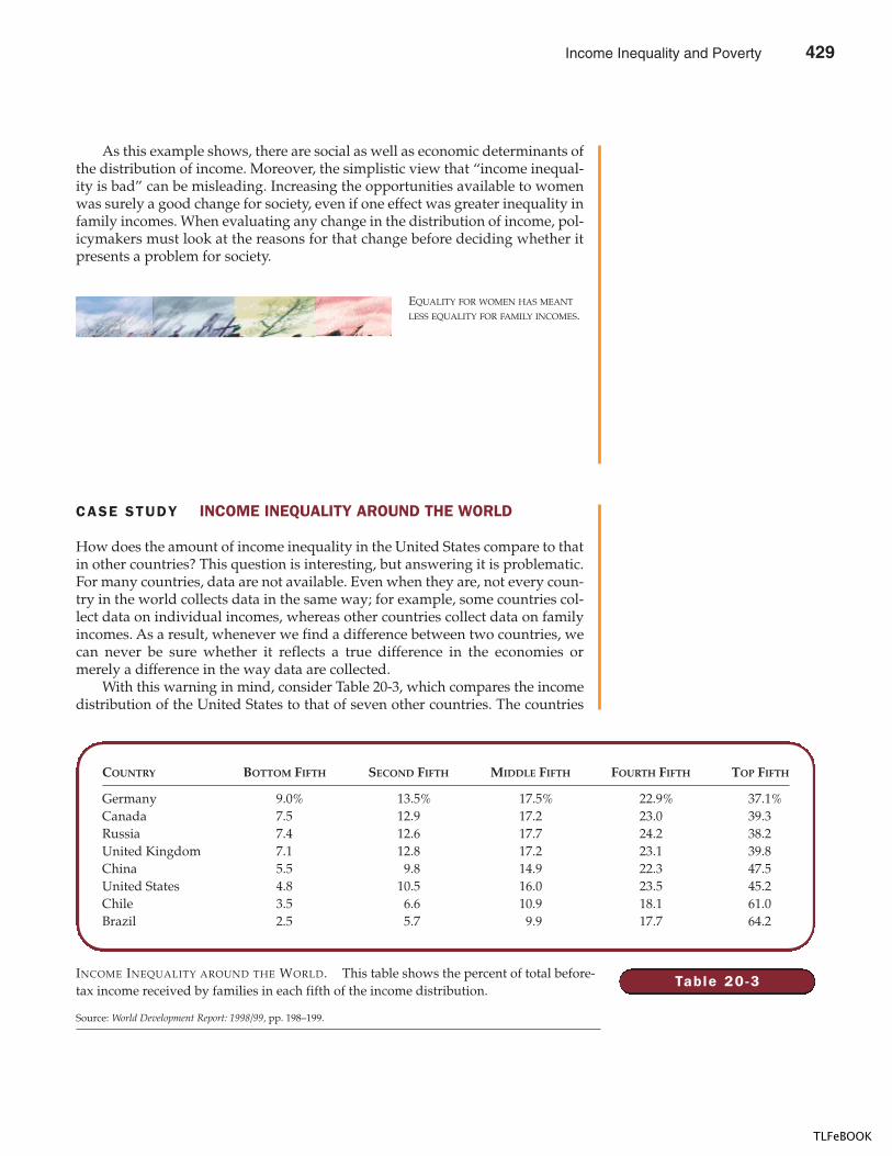
CHAPTER 20 INCOME INEQUALITY AND POVERTY 441
As this example shows, there are social as well as economic determinants ofthe distribution of income. Moreover, the simplistic view that “income inequal-ity is bad” can be misleading. Increasing the opportunities available to womenwas surely a good change for society, even if one effect was greater inequality infamily incomes. When evaluating any change in the distribution of income, pol-icymakers must look at the reasons for that change before deciding whether itpresents a problem for society.
CASE STUDY INCOME INEQUALITY AROUND THE WORLD
How does the amount of income inequality in the United States compare to thatin other countries? This question is interesting, but answering it is problematic.For many countries, data are not available. Even when they are, not every coun-try in the world collects data in the same way; for example, some countries col-lect data on individual incomes, whereas other countries collect data on familyincomes. As a result, whenever we find a difference between two countries, wecan never be sure whether it reflects a true difference in the economies ormerely a difference in the way data are collected.
With this warning in mind, consider Table 20-3, which compares the incomedistribution of the United States to that of seven other countries. The countries
EQUALITY FOR WOMEN HAS MEANT
LESS EQUALITY FOR FAMILY INCOMES.
Table 20 -3
COUNTRY BOTTOM FIFTH SECOND FIFTH MIDDLE FIFTH FOURTH FIFTH TOP FIFTH
Germany 9.0% 13.5% 17.5% 22.9% 37.1%Canada 7.5 12.9 17.2 23.0 39.3Russia 7.4 12.6 17.7 24.2 38.2United Kingdom 7.1 12.8 17.2 23.1 39.8China 5.5 9.8 14.9 22.3 47.5United States 4.8 10.5 16.0 23.5 45.2Chile 3.5 6.6 10.9 18.1 61.0Brazil 2.5 5.7 9.9 17.7 64.2
INCOME INEQUALITY AROUND THE WORLD. This table shows the percent of total before-tax income received by families in each fifth of the income distribution.
Source: World Development Report: 1998/99, pp. 198–199.
Income Inequality and Poverty 429
TLFeBOOK
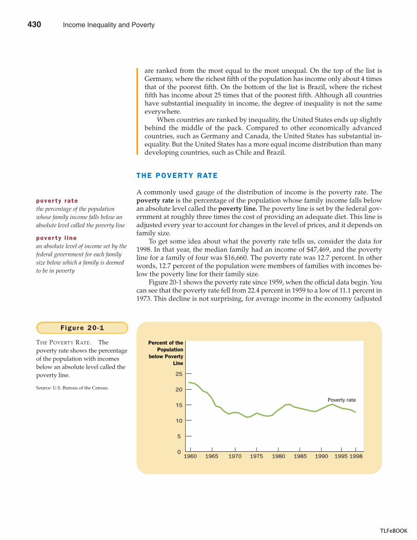
442 PART SIX THE ECONOMICS OF LABOR MARKETS
are ranked from the most equal to the most unequal. On the top of the list isGermany, where the richest fifth of the population has income only about 4 timesthat of the poorest fifth. On the bottom of the list is Brazil, where the richestfifth has income about 25 times that of the poorest fifth. Although all countrieshave substantial inequality in income, the degree of inequality is not the sameeverywhere.
When countries are ranked by inequality, the United States ends up slightlybehind the middle of the pack. Compared to other economically advancedcountries, such as Germany and Canada, the United States has substantial in-equality. But the United States has a more equal income distribution than manydeveloping countries, such as Chile and Brazil.
THE POVERTY RATE
A commonly used gauge of the distribution of income is the poverty rate. Thepoverty rate is the percentage of the population whose family income falls belowan absolute level called the poverty line. The poverty line is set by the federal gov-ernment at roughly three times the cost of providing an adequate diet. This line isadjusted every year to account for changes in the level of prices, and it depends onfamily size.
To get some idea about what the poverty rate tells us, consider the data for1998. In that year, the median family had an income of $47,469, and the povertyline for a family of four was $16,660. The poverty rate was 12.7 percent. In otherwords, 12.7 percent of the population were members of families with incomes be-low the poverty line for their family size.
Figure 20-1 shows the poverty rate since 1959, when the official data begin. Youcan see that the poverty rate fell from 22.4 percent in 1959 to a low of 11.1 percent in1973. This decline is not surprising, for average income in the economy (adjusted
pover ty l inean absolute level of income set by thefederal government for each familysize below which a family is deemedto be in poverty
Percent of thePopulation
below PovertyLine
1960 1965 1970 1975 1980 1985 1990 1995 19980
5
10
15
20
25
Poverty rate
Figure 20 -1
THE POVERTY RATE. Thepoverty rate shows the percentageof the population with incomesbelow an absolute level called thepoverty line.
Source: U.S. Bureau of the Census.
pover ty ratethe percentage of the populationwhose family income falls below anabsolute level called the poverty line
430 Income Inequality and Poverty
TLFeBOOK
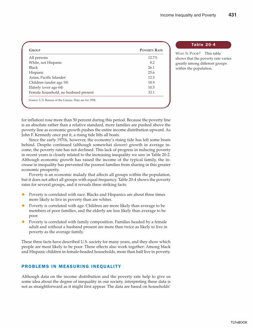
CHAPTER 20 INCOME INEQUALITY AND POVERTY 443
for inflation) rose more than 50 percent during this period. Because the poverty lineis an absolute rather than a relative standard, more families are pushed above thepoverty line as economic growth pushes the entire income distribution upward. AsJohn F. Kennedy once put it, a rising tide lifts all boats.
Since the early 1970s, however, the economy’s rising tide has left some boatsbehind. Despite continued (although somewhat slower) growth in average in-come, the poverty rate has not declined. This lack of progress in reducing povertyin recent years is closely related to the increasing inequality we saw in Table 20-2.Although economic growth has raised the income of the typical family, the in-crease in inequality has prevented the poorest families from sharing in this greatereconomic prosperity.
Poverty is an economic malady that affects all groups within the population,but it does not affect all groups with equal frequency. Table 20-4 shows the povertyrates for several groups, and it reveals three striking facts:
� Poverty is correlated with race. Blacks and Hispanics are about three timesmore likely to live in poverty than are whites.
� Poverty is correlated with age. Children are more likely than average to bemembers of poor families, and the elderly are less likely than average to bepoor.
� Poverty is correlated with family composition. Families headed by a femaleadult and without a husband present are more than twice as likely to live inpoverty as the average family.
These three facts have described U.S. society for many years, and they show whichpeople are most likely to be poor. These effects also work together: Among blackand Hispanic children in female-headed households, more than half live in poverty.
PROBLEMS IN MEASURING INEQUALITY
Although data on the income distribution and the poverty rate help to give ussome idea about the degree of inequality in our society, interpreting these data isnot as straightforward as it might first appear. The data are based on households’
Table 20 -4
WHO IS POOR? This tableshows that the poverty rate variesgreatly among different groupswithin the population.
GROUP POVERTY RATE
All persons 12.7%White, not Hispanic 8.2Black 26.1Hispanic 25.6Asian, Pacific Islander 12.5Children (under age 18) 18.9Elderly (over age 64) 10.5Female household, no husband present 33.1
Source: U.S. Bureau of the Census. Data are for 1998.
Income Inequality and Poverty 431
TLFeBOOK
444 PART SIX THE ECONOMICS OF LABOR MARKETS
annual incomes. What people care about, however, is not their incomes but theirability to maintain a good standard of living. For various reasons, data on the in-come distribution and the poverty rate give an incomplete picture of inequality inliving standards. We examine these reasons below.
In -K ind Trans fe rs Measurements of the distribution of income and thepoverty rate are based on families’ money income. Through various governmentprograms, however, the poor receive many nonmonetary items, including foodstamps, housing vouchers, and medical services. Transfers to the poor given in theform of goods and services rather than cash are called in-kind transfers. Standardmeasurements of the degree of inequality do not take account of these in-kindtransfers.
Because in-kind transfers are received mostly by the poorest members of soci-ety, the failure to include in-kind transfers as part of income greatly affects themeasured poverty rate. According to a study by the Census Bureau, if in-kindtransfers were included in income at their market value, the number of families inpoverty would be about 10 percent lower than the standard data indicate.
The important role of in-kind transfers makes evaluating changes in povertymore difficult. Over time, as public policies to help the poor evolve, the composi-tion of assistance between cash and in-kind transfers changes. Some of the fluctu-ations in the measured poverty rate, therefore, reflect the form of governmentassistance rather than the true extent of economic deprivation.
The Economic L i fe Cyc le Incomes vary predictably over people’s lives.A young worker, especially one in school, has a low income. Income rises as theworker gains maturity and experience, peaks at around age 50, and then fallssharply when the worker retires at around age 65. This regular pattern of incomevariation is called the life cycle.
Because people can borrow and save to smooth out life cycle changes in in-come, their standard of living in any year depends more on lifetime income thanon that year’s income. The young often borrow, perhaps to go to school or to buya house, and then repay these loans later when their incomes rise. People havetheir highest saving rates when they are middle-aged. Because people can save inanticipation of retirement, the large declines in incomes at retirement need not leadto similar declines in the standard of living.
This normal life cycle pattern causes inequality in the distribution of annualincome, but it does not represent true inequality in living standards. To gaugethe inequality of living standards in our society, the distribution of lifetime in-comes is more relevant than the distribution of annual incomes. Unfortunately,data on lifetime incomes are not readily available. When looking at any data oninequality, however, it is important to keep the life cycle in mind. Because a per-son’s lifetime income smooths out the highs and lows of the life cycle, lifetime in-comes are surely more equally distributed across the population than are annualincomes.
Trans i to r y versus Permanent Income Incomes vary over people’slives not only because of predictable life cycle variation but also because of ran-dom and transitory forces. One year a frost kills off the Florida orange crop, andFlorida orange growers see their incomes fall temporarily. At the same time, the
in -k ind t rans ferstransfers to the poor given in theform of goods and services ratherthan cash
l i fe cyc lethe regular pattern of incomevariation over a person’s life
432 Income Inequality and Poverty
TLFeBOOK
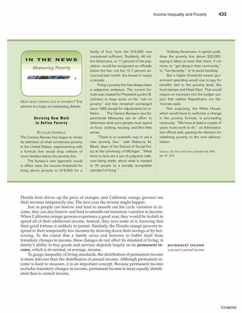
CHAPTER 20 INCOME INEQUALITY AND POVERTY 445
Florida frost drives up the price of oranges, and California orange growers seetheir incomes temporarily rise. The next year the reverse might happen.
Just as people can borrow and lend to smooth out life cycle variation in in-come, they can also borrow and lend to smooth out transitory variation in income.When California orange growers experience a good year, they would be foolish tospend all of their additional income. Instead, they save some of it, knowing thattheir good fortune is unlikely to persist. Similarly, the Florida orange growers re-spond to their temporarily low incomes by drawing down their savings or by bor-rowing. To the extent that a family saves and borrows to buffer itself fromtransitory changes in income, these changes do not affect its standard of living. Afamily’s ability to buy goods and services depends largely on its permanent in-come, which is its normal, or average, income.
To gauge inequality of living standards, the distribution of permanent incomeis more relevant than the distribution of annual income. Although permanent in-come is hard to measure, it is an important concept. Because permanent incomeexcludes transitory changes in income, permanent income is more equally distrib-uted than is current income.
permanent incomea person’s normal income
HOW MANY PEOPLE LIVE IN POVERTY? THE
answer is a topic of continuing debate.
D e v i s i n g N e w M a t ht o D e f i n e P o v e r t y
BY LOUIS UCHITELLE
The Census Bureau has begun to reviseits definition of what constitutes povertyin the United States, experimenting witha formula that would drop millions ofmore families below the poverty line.
The bureau’s new approach wouldin effect raise the income threshold forliving above poverty to $19,500 for a
family of four, from the $16,600 nowconsidered sufficient. Suddenly, 46 mil-lion Americans, or 17 percent of the pop-ulation, would be recognized as officiallybelow the line, not the 12.7 percent an-nounced last month, the lowest in nearlya decade. . . .
Fixing a poverty line has always beena subjective endeavor. The current for-mula was created for President Lyndon B.Johnson to keep score on his “war onpoverty” and has remained unchangedsince 1965 except for adjustments for in-flation. . . . The Census Bureau’s new Ex-perimental Measures are an effort todetermine what poor people must spendon food, clothing, housing, and life’s littleextras.
“There is no scientific way to set anew poverty line,” said Rebecca M.Blank, dean of the School of Social Pol-icy at the University of Michigan. “Whatthere is here are a set of judgment calls,now being made, about what is neededto lift people to a socially acceptablestandard of living.” . . .
Ordinary Americans, in opinion polls,draw the poverty line above $20,000,saying it takes at least that much, if notmore, to “get along in their community,”to “live decently,” or to avoid hardship.
But a higher threshold means gov-ernment spending would rise to pay forbenefits tied to the poverty level, likefood stamps and Head Start. That wouldrequire an incursion into the budget sur-plus that neither Republicans nor De-mocrats seek.
Not surprising, the White House,which would have to authorize a changein the poverty formula, is proceedingcautiously. “We have at least a couple ofyears more work to do,” an Administra-tion official said, passing the decision forredefining poverty to the next adminis-tration.
SOURCE: The New York Times, October 18, 1999,pp. A1, A14.
IN THE NEWS
Measuring Poverty
Income Inequality and Poverty 433
TLFeBOOK
446 PART SIX THE ECONOMICS OF LABOR MARKETS
ECONOMIC MOBIL ITY
People sometimes speak of “the rich” and “the poor” as if these groups consistedof the same families year after year. In fact, this is not at all the case. Economic mo-bility, the movement of people among income classes, is substantial in the U.S.economy. Movements up the income ladder can be due to good luck or hard work,and movements down the ladder can be due to bad luck or laziness. Some of thismobility reflects transitory variation in income, while some reflects more persis-tent changes in income.
Because economic mobility is so great, many of those below the poverty lineare there only temporarily. Poverty is a long-term problem for relatively few fam-ilies. In a typical ten-year period, about one in four families falls below the povertyline in at least one year. Yet fewer than 3 percent of families are poor for eight ormore years. Because it is likely that the temporarily poor and the persistently poorface different problems, policies that aim to combat poverty need to distinguishbetween these groups.
Another way to gauge economic mobility is the persistence of economic suc-cess from generation to generation. Economists who have studied this topic findsubstantial mobility. If a father earns 20 percent above his generation’s average in-come, his son will most likely earn 8 percent above his generation’s average in-come. There is almost no correlation between the income of a grandfather and theincome of a grandson. There is much truth to the old saying, “From shirtsleeves toshirtsleeves in three generations.”
One result of this great economic mobility is that the U.S. economy is filledwith self-made millionaires (as well as with heirs who squandered the fortunesthey inherited). According to estimates for 1996, about 2.7 million households inthe United States had net worth (assets minus debts) that exceeded $1 million.These households represented the richest 2.8 percent of the population. About fourout of five of these millionaires made their money on their own, such as by start-ing and building a business or by climbing the corporate ladder. Only one in fivemillionaires inherited their fortunes.
QUICK QUIZ: What does the poverty rate measure? � Describe three potential problems in interpreting the measured poverty rate.
THE POLIT ICAL PHILOSOPHYOF REDISTRIBUTING INCOME
We have just seen how the economy’s income is distributed and have consideredsome of the problems in interpreting measured inequality. This discussion was pos-itive in the sense that it merely described the world as it is. We now turn to the nor-mative question facing policymakers: What should the government do abouteconomic inequality?
This question is not just about economics. Economic analysis alone cannot tellus whether policymakers should try to make our society more egalitarian. Ourviews on this question are, to a large extent, a matter of political philosophy. Yet
434 Income Inequality and Poverty
TLFeBOOK
CHAPTER 20 INCOME INEQUALITY AND POVERTY 447
because the government’s role in redistributing income is central to so many de-bates over economic policy, here we digress from economic science to consider abit of political philosophy.
UTIL ITARIANISM
A prominent school of thought in political philosophy is utilitarianism. Thefounders of utilitarianism are the English philosophers Jeremy Bentham (1748–1832)and John Stuart Mill (1806–1873). To a large extent, the goal of utilitarians is to ap-ply the logic of individual decisionmaking to questions concerning morality andpublic policy.
The starting point of utilitarianism is the notion of utility—the level of happi-ness or satisfaction that a person receives from his or her circumstances. Utility isa measure of well-being and, according to utilitarians, is the ultimate objective ofall public and private actions. The proper goal of the government, they claim, is tomaximize the sum of utility of everyone in society.
The utilitarian case for redistributing income is based on the assumption of di-minishing marginal utility. It seems reasonable that an extra dollar of income to apoor person provides that person with more additional utility than does an extradollar to a rich person. In other words, as a person’s income rises, the extra well-being derived from an additional dollar of income falls. This plausible assumption,together with the utilitarian goal of maximizing total utility, implies that the gov-ernment should try to achieve a more equal distribution of income.
The argument is simple. Imagine that Peter and Paul are the same, except thatPeter earns $80,000 and Paul earns $20,000. In this case, taking a dollar from Peterto pay Paul will reduce Peter’s utility and raise Paul’s utility. But, because of di-minishing marginal utility, Peter’s utility falls by less than Paul’s utility rises.Thus, this redistribution of income raises total utility, which is the utilitarian’sobjective.
At first, this utilitarian argument might seem to imply that the governmentshould continue to redistribute income until everyone in society has exactly thesame income. Indeed, that would be the case if the total amount of income—$100,000 in our example—were fixed. But, in fact, it is not. Utilitarians reject com-plete equalization of incomes because they accept one of the Ten Principles ofEconomics presented in Chapter 1: People respond to incentives.
To take from Peter to pay Paul, the government must pursue policies that re-distribute income, such as the U.S. federal income tax and welfare system. Underthese policies, people with high incomes pay high taxes, and people with low in-comes receive income transfers. Yet, as we have seen in Chapters 8 and 12, taxesdistort incentives and cause deadweight losses. If the government takes away ad-ditional income a person might earn through higher income taxes or reducedtransfers, both Peter and Paul have less incentive to work hard. As they work less,society’s income falls, and so does total utility. The utilitarian government has tobalance the gains from greater equality against the losses from distorted incen-tives. To maximize total utility, therefore, the government stops short of makingsociety fully egalitarian.
A famous parable sheds light on the utilitarian’s logic. Imagine that Peter andPaul are thirsty travelers trapped at different places in the desert. Peter’s oasis hasmuch water; Paul’s has little. If the government could transfer water from one oasis
ut i l i ta r ian ismthe political philosophy according towhich the government should choosepolicies to maximize the total utilityof everyone in society
ut i l i tya measure of happiness orsatisfaction
Income Inequality and Poverty 435
TLFeBOOK
448 PART SIX THE ECONOMICS OF LABOR MARKETS
to the other without cost, it would maximize total utility from water by equalizingthe amount in the two places. But suppose that the government has only a leakybucket. As it tries to move water from one place to the other, some of the water islost in transit. In this case, a utilitarian government might still try to move some wa-ter from Peter to Paul, depending on how thirsty Paul is and how leaky the bucketis. But, with only a leaky bucket at its disposal, a utilitarian government will not tryto reach complete equality.
LIBERALISM
A second way of thinking about inequality might be called liberalism. Philoso-pher John Rawls develops this view in his book A Theory of Justice. This book wasfirst published in 1971, and it quickly became a classic in political philosophy.
Rawls begins with the premise that a society’s institutions, laws, and policiesshould be just. He then takes up the natural question: How can we, the membersof society, ever agree on what justice means? It might seem that every person’spoint of view is inevitably based on his or her particular circumstances—whetherhe or she is talented or less talented, diligent or lazy, educated or less educated,born to a wealthy family or a poor one. Could we ever objectively determine whata just society would be?
To answer this question, Rawls proposes the following thought experiment.Imagine that before any of us is born, we all get together for a meeting to designthe rules that govern society. At this point, we are all ignorant about the station inlife each of us will end up filling. In Rawls’s words, we are sitting in an “originalposition” behind a “veil of ignorance.” In this original position, Rawls argues, wecan choose a just set of rules for society because we must consider how those ruleswill affect every person. As Rawls puts it, “Since all are similarly situated and noone is able to design principles to favor his particular conditions, the principles ofjustice are the result of fair agreement or bargain.” Designing public policies andinstitutions in this way allows us to be objective about what policies are just.
Rawls then considers what public policy designed behind this veil of igno-rance would try to achieve. In particular, he considers what income distribution aperson would consider just if that person did not know whether he or she wouldend up at the top, bottom, or middle of the distribution. Rawls argues that a per-son in the original position would be especially concerned about the possibility ofbeing at the bottom of the income distribution. In designing public policies, there-fore, we should aim to raise the welfare of the worst-off person in society. That is,rather than maximizing the sum of everyone’s utility, as a utilitarian would do,Rawls would maximize the minimum utility. Rawls’s rule is called the maximincriterion.
Because the maximin criterion emphasizes the least fortunate person in soci-ety, it justifies public policies aimed at equalizing the distribution of income. Bytransferring income from the rich to the poor, society raises the well-being of theleast fortunate. The maximin criterion would not, however, lead to a completelyegalitarian society. If the government promised to equalize incomes completely,people would have no incentive to work hard, society’s total income would fallsubstantially, and the least fortunate person would be worse off. Thus, the max-imin criterion still allows disparities in income, because such disparities can im-prove incentives and thereby raise society’s ability to help the poor. Nonetheless,
l ibera l ismthe political philosophy according towhich the government should choosepolicies deemed to be just, asevaluated by an impartial observerbehind a “veil of ignorance”
maximin cr i te r ionthe claim that the government shouldaim to maximize the well-being ofthe worst-off person in society
436 Income Inequality and Poverty
TLFeBOOK
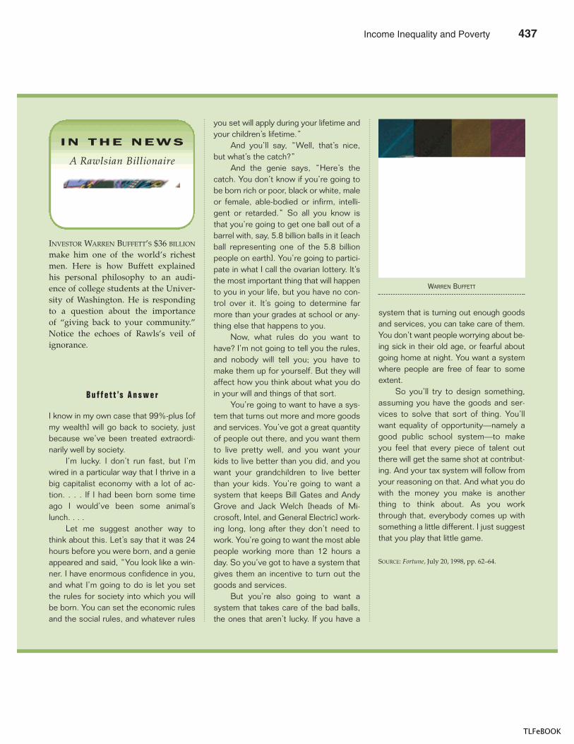
CHAPTER 20 INCOME INEQUALITY AND POVERTY 449
INVESTOR WARREN BUFFETT’S $36 BILLION
make him one of the world’s richestmen. Here is how Buffett explainedhis personal philosophy to an audi-ence of college students at the Univer-sity of Washington. He is respondingto a question about the importanceof “giving back to your community.”Notice the echoes of Rawls’s veil ofignorance.
B u f f e t t ’s A n s w e r
I know in my own case that 99%-plus [ofmy wealth] will go back to society, justbecause we’ve been treated extraordi-narily well by society.
I’m lucky. I don’t run fast, but I’mwired in a particular way that I thrive in abig capitalist economy with a lot of ac-tion. . . . If I had been born some timeago I would’ve been some animal’slunch. . . .
Let me suggest another way tothink about this. Let’s say that it was 24hours before you were born, and a genieappeared and said, “You look like a win-ner. I have enormous confidence in you,and what I’m going to do is let you setthe rules for society into which you willbe born. You can set the economic rulesand the social rules, and whatever rules
you set will apply during your lifetime andyour children’s lifetime.”
And you’ll say, “Well, that’s nice,but what’s the catch?”
And the genie says, “Here’s thecatch. You don’t know if you’re going tobe born rich or poor, black or white, maleor female, able-bodied or infirm, intelli-gent or retarded.” So all you know isthat you’re going to get one ball out of abarrel with, say, 5.8 billion balls in it [eachball representing one of the 5.8 billionpeople on earth]. You’re going to partici-pate in what I call the ovarian lottery. It’sthe most important thing that will happento you in your life, but you have no con-trol over it. It’s going to determine farmore than your grades at school or any-thing else that happens to you.
Now, what rules do you want tohave? I’m not going to tell you the rules,and nobody will tell you; you have tomake them up for yourself. But they willaffect how you think about what you doin your will and things of that sort.
You’re going to want to have a sys-tem that turns out more and more goodsand services. You’ve got a great quantityof people out there, and you want themto live pretty well, and you want yourkids to live better than you did, and youwant your grandchildren to live betterthan your kids. You’re going to want asystem that keeps Bill Gates and AndyGrove and Jack Welch [heads of Mi-crosoft, Intel, and General Electric] work-ing long, long after they don’t need towork. You’re going to want the most ablepeople working more than 12 hours aday. So you’ve got to have a system thatgives them an incentive to turn out thegoods and services.
But you’re also going to want asystem that takes care of the bad balls,the ones that aren’t lucky. If you have a
system that is turning out enough goodsand services, you can take care of them.You don’t want people worrying about be-ing sick in their old age, or fearful aboutgoing home at night. You want a systemwhere people are free of fear to someextent.
So you’ll try to design something,assuming you have the goods and ser-vices to solve that sort of thing. You’llwant equality of opportunity—namely agood public school system—to makeyou feel that every piece of talent outthere will get the same shot at contribut-ing. And your tax system will follow fromyour reasoning on that. And what you dowith the money you make is anotherthing to think about. As you workthrough that, everybody comes up withsomething a little different. I just suggestthat you play that little game.
SOURCE: Fortune, July 20, 1998, pp. 62–64.
IN THE NEWS
A Rawlsian Billionaire
WARREN BUFFETT
Income Inequality and Poverty 437
TLFeBOOK
450 PART SIX THE ECONOMICS OF LABOR MARKETS
because Rawls’s philosophy puts weight on only the least fortunate members ofsociety, it calls for more income redistribution than does utilitarianism.
Rawls’s views are controversial, but the thought experiment he proposes hasmuch appeal. In particular, this thought experiment allows us to consider the re-distribution of income as a form of social insurance. That is, from the perspective ofthe original position behind the veil of ignorance, income redistribution is like aninsurance policy. Homeowners buy fire insurance to protect themselves from therisk of their housing burning down. Similarly, when we as a society choose policiesthat tax the rich to supplement the incomes of the poor, we are all insuring our-selves against the possibility that we might have been a member of a poor family.Because people dislike risk, we should be happy to have been born into a societythat provides us this insurance.
It is not at all clear, however, that rational people behind the veil of ignorancewould truly be so averse to risk as to follow the maximin criterion. Indeed, be-cause a person in the original position might end up anywhere in the distributionof outcomes, he or she might treat all possible outcomes equally when designingpublic policies. In this case, the best policy behind the veil of ignorance would beto maximize the average utility of members of society, and the resulting notion ofjustice would be more utilitarian than Rawlsian.
LIBERTARIANISM
A third view of inequality is called libertarianism. The two views we have con-sidered so far—utilitarianism and liberalism—both view the total income of soci-ety as a shared resource that a social planner can freely redistribute to achievesome social goal. By contrast, libertarians argue that society itself earns no in-come—only individual members of society earn income. According to libertarians,the government should not take from some individuals and give to others in orderto achieve any particular distribution of income.
For instance, philosopher Robert Nozick writes the following in his famous1974 book Anarchy, State and Utopia:
We are not in the position of children who have been given portions of pie bysomeone who now makes last minute adjustments to rectify careless cutting.There is no central distribution, no person or group entitled to control all theresources, jointly deciding how they are to be doled out. What each person gets,he gets from others who give to him in exchange for something, or as a gift. In afree society, diverse persons control different resources, and new holdings ariseout of the voluntary exchanges and actions of persons.
Whereas utilitarians and liberals try to judge what amount of inequality is desir-able in a society, Nozick denies the validity of this very question.
The libertarian alternative to evaluating economic outcomes is to evaluate theprocess by which these outcomes arise. When the distribution of income is achievedunfairly—for instance, when one person steals from another—the government hasthe right and duty to remedy the problem. But, as long as the process determiningthe distribution of income is just, the resulting distribution is fair, no matter howunequal.
Nozick criticizes Rawls’s liberalism by drawing an analogy between the dis-tribution of income in society and the distribution of grades in a course. Supposeyou were asked to judge the fairness of the grades in the economics course you are
l iber tar ian ismthe political philosophy accordingto which the government shouldpunish crimes and enforce voluntaryagreements but not redistributeincome
438 Income Inequality and Poverty
TLFeBOOK
CHAPTER 20 INCOME INEQUALITY AND POVERTY 451
now taking. Would you imagine yourself behind a veil of ignorance and choose agrade distribution without knowing the talents and efforts of each student? Orwould you ensure that the process of assigning grades to students is fair withoutregard for whether the resulting distribution is equal or unequal? For the case ofgrades at least, the libertarian emphasis on process over outcomes is compelling.
Libertarians conclude that equality of opportunities is more important thanequality of incomes. They believe that the government should enforce individualrights to ensure that everyone has the same opportunity to use his or her talentsand achieve success. Once these rules of the game are established, the governmenthas no reason to alter the resulting distribution of income.
QUICK QUIZ: Pam earns more than Pauline. Someone proposes taxing Pam in order to supplement Pauline’s income. How would a utilitarian, a liberal, and a libertarian evaluate this proposal?
POLICIES TO REDUCE POVERTY
As we have just seen, political philosophers hold various views about what role thegovernment should take in altering the distribution of income. Political debateamong the larger population of voters reflects a similar disagreement. Despite thesecontinuing debates, however, most people believe that, at the very least, the gov-ernment should try to help those most in need. According to a popular metaphor,the government should provide a “safety net” to prevent any citizen from fallingtoo far.
Poverty is one of the most difficult problems that policymakers face. Poor fam-ilies are more likely than the overall population to experience homelessness, drugdependency, domestic violence, health problems, teenage pregnancy, illiteracy, un-employment, and low educational attainment. Members of poor families are bothmore likely to commit crimes and more likely to be victims of crimes. Although itis hard to separate the causes of poverty from the effects, there is no doubt thatpoverty is associated with various economic and social ills.
Suppose that you were a policymaker in the government, and your goal wasto reduce the number of people living in poverty. How would you achieve thisgoal? Here we consider some of the policy options that you might consider. Al-though each of these options does help some people escape poverty, none of themis perfect, and deciding which is best is not easy.
MINIMUM-WAGE LAWS
Laws setting a minimum wage that employers can pay workers are a perennialsource of debate. Advocates view the minimum wage as a way of helping theworking poor without any cost to the government. Critics view it as hurting thoseit is intended to help.
The minimum wage is easily understood using the tools of supply and demand,as we first saw in Chapter 6. For workers with low levels of skill and experience, a
Income Inequality and Poverty 439
TLFeBOOK
452 PART SIX THE ECONOMICS OF LABOR MARKETS
high minimum wage forces the wage above the level that balances supply and de-mand. It therefore raises the cost of labor to firms and reduces the quantity of laborthat those firms demand. The result is higher unemployment among those groups ofworkers affected by the minimum wage. Although those workers who remain em-ployed benefit from a higher wage, those who might have been employed at a lowerwage are worse off.
The magnitude of these effects depends crucially on the elasticity of demand.Advocates of a high minimum wage argue that the demand for unskilled labor isrelatively inelastic, so that a high minimum wage depresses employment onlyslightly. Critics of the minimum wage argue that labor demand is more elastic, es-pecially in the long run when firms can adjust employment and production morefully. They also note that many minimum-wage workers are teenagers frommiddle-class families, so that a high minimum wage is imperfectly targeted as apolicy for helping the poor.
WELFARE
One way to raise the living standards of the poor is for the government to supple-ment their incomes. The primary way in which the government does this isthrough the welfare system. Welfare is a broad term that encompasses variousgovernment programs. Temporary Assistance for Needy Families (formerly calledAid to Families with Dependent Children) is a program that assists families wherethere are children but no adult able to support the family. In a typical family re-ceiving such assistance, the father is absent, and the mother is at home raisingsmall children. Another welfare program is Supplemental Security Income (SSI),which provides assistance to the poor who are sick or disabled. Note that for bothof these welfare programs, a poor person cannot qualify for assistance simply byhaving a low income. He or she must also establish some additional “need,” suchas small children or a disability.
A common criticism of welfare programs is that they create incentives forpeople to become “needy.” For example, these programs may encourage familiesto break up, for many families qualify for financial assistance only if the fatheris absent. The programs may also encourage illegitimate births, for many poor,single women qualify for assistance only if they have children. Because poor,single mothers are such an important part of the poverty problem and becausewelfare programs seem to raise the number of poor, single mothers, critics of thewelfare system assert that these policies exacerbate the very problems they aresupposed to cure. As a result of these arguments, the welfare system was re-vised in a 1996 law that limited the amount of time recipients could stay onwelfare.
How severe are these potential problems with the welfare system? No oneknows for sure. Proponents of the welfare system point out that being a poor, sin-gle mother on welfare is a difficult existence at best, and they are skeptical thatmany people would be encouraged to pursue such a life if it were not thrust uponthem. Moreover, trends over time do not support the view that the decline of thetwo-parent family is largely a symptom of the welfare system, as the system’scritics sometimes claim. Since the early 1970s, welfare benefits (adjusted for infla-tion) have declined, yet the percentage of children living with only one parent hasrisen.
wel fa regovernment programs thatsupplement the incomes of the needy
440 Income Inequality and Poverty
TLFeBOOK
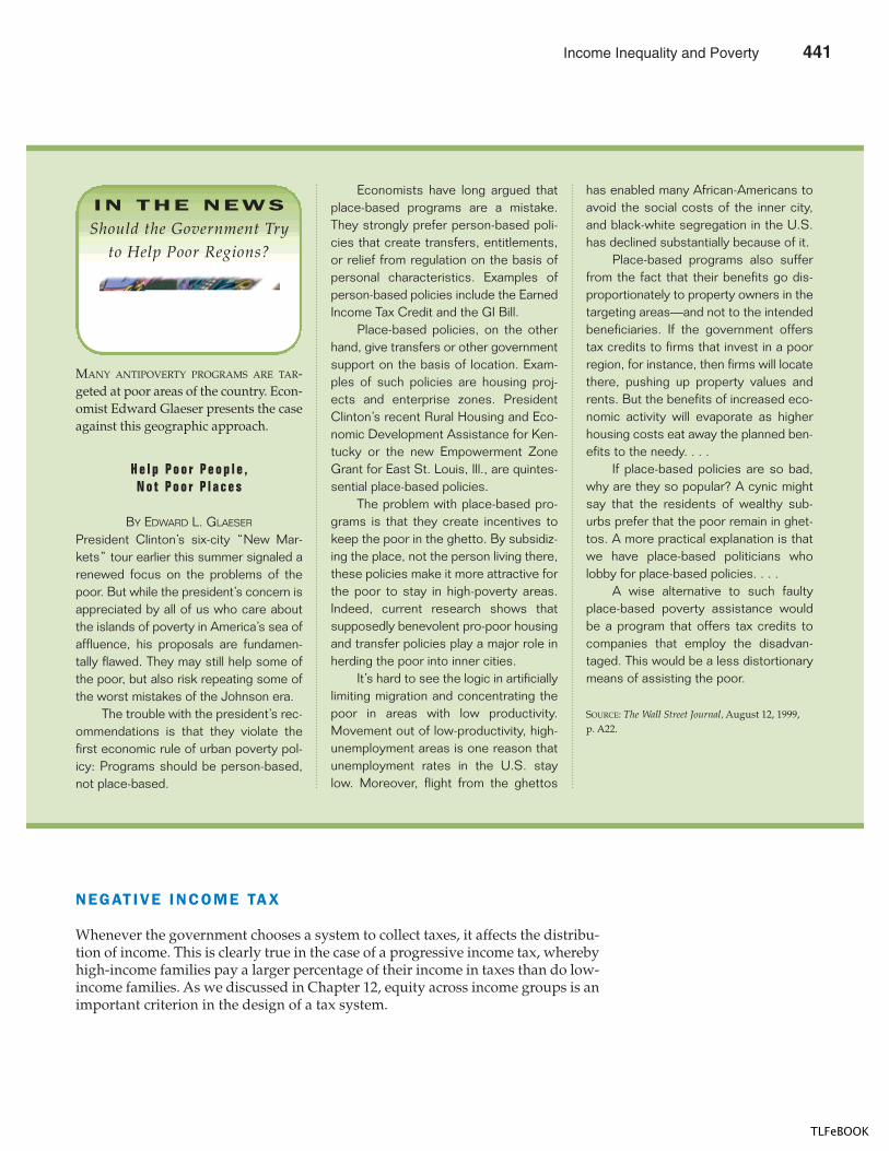
CHAPTER 20 INCOME INEQUALITY AND POVERTY 453
NEGATIVE INCOME TAX
Whenever the government chooses a system to collect taxes, it affects the distribu-tion of income. This is clearly true in the case of a progressive income tax, wherebyhigh-income families pay a larger percentage of their income in taxes than do low-income families. As we discussed in Chapter 12, equity across income groups is animportant criterion in the design of a tax system.
MANY ANTIPOVERTY PROGRAMS ARE TAR-geted at poor areas of the country. Econ-omist Edward Glaeser presents the caseagainst this geographic approach.
H e l p P o o r P e o p l e ,N o t P o o r P l a c e s
BY EDWARD L. GLAESER
President Clinton’s six-city “New Mar-kets” tour earlier this summer signaled arenewed focus on the problems of thepoor. But while the president’s concern isappreciated by all of us who care aboutthe islands of poverty in America’s sea ofaffluence, his proposals are fundamen-tally flawed. They may still help some ofthe poor, but also risk repeating some ofthe worst mistakes of the Johnson era.
The trouble with the president’s rec-ommendations is that they violate thefirst economic rule of urban poverty pol-icy: Programs should be person-based,not place-based.
Economists have long argued thatplace-based programs are a mistake.They strongly prefer person-based poli-cies that create transfers, entitlements,or relief from regulation on the basis ofpersonal characteristics. Examples ofperson-based policies include the EarnedIncome Tax Credit and the GI Bill.
Place-based policies, on the otherhand, give transfers or other governmentsupport on the basis of location. Exam-ples of such policies are housing proj-ects and enterprise zones. PresidentClinton’s recent Rural Housing and Eco-nomic Development Assistance for Ken-tucky or the new Empowerment ZoneGrant for East St. Louis, Ill., are quintes-sential place-based policies.
The problem with place-based pro-grams is that they create incentives tokeep the poor in the ghetto. By subsidiz-ing the place, not the person living there,these policies make it more attractive forthe poor to stay in high-poverty areas.Indeed, current research shows thatsupposedly benevolent pro-poor housingand transfer policies play a major role inherding the poor into inner cities.
It’s hard to see the logic in artificiallylimiting migration and concentrating thepoor in areas with low productivity.Movement out of low-productivity, high-unemployment areas is one reason thatunemployment rates in the U.S. staylow. Moreover, flight from the ghettos
has enabled many African-Americans toavoid the social costs of the inner city,and black-white segregation in the U.S.has declined substantially because of it.
Place-based programs also sufferfrom the fact that their benefits go dis-proportionately to property owners in thetargeting areas—and not to the intendedbeneficiaries. If the government offerstax credits to firms that invest in a poorregion, for instance, then firms will locatethere, pushing up property values andrents. But the benefits of increased eco-nomic activity will evaporate as higherhousing costs eat away the planned ben-efits to the needy. . . .
If place-based policies are so bad,why are they so popular? A cynic mightsay that the residents of wealthy sub-urbs prefer that the poor remain in ghet-tos. A more practical explanation is thatwe have place-based politicians wholobby for place-based policies. . . .
A wise alternative to such faultyplace-based poverty assistance wouldbe a program that offers tax credits tocompanies that employ the disadvan-taged. This would be a less distortionarymeans of assisting the poor.
SOURCE: The Wall Street Journal, August 12, 1999,p. A22.
IN THE NEWS
Should the Government Tryto Help Poor Regions?
Income Inequality and Poverty 441
TLFeBOOK
454 PART SIX THE ECONOMICS OF LABOR MARKETS
Many economists have advocated supplementing the income of the poor us-ing a negative income tax. According to this policy, every family would report itsincome to the government. High-income families would pay a tax based on theirincomes. Low-income families would receive a subsidy. In other words, theywould “pay” a “negative tax.”
For example, suppose the government used the following formula to computea family’s tax liability:
Taxes owed � (1/3 of income) � $10,000.
In this case, a family that earned $60,000 would pay $10,000 in taxes, and a familythat earned $90,000 would pay $20,000 in taxes. A family that earned $30,000would owe nothing. And a family that earned $15,000 would “owe” �$5,000. Inother words, the government would send this family a check for $5,000.
Under a negative income tax, poor families would receive financial assistancewithout having to demonstrate need. The only qualification required to receive as-sistance would be a low income. Depending on one’s point of view, this featurecan be either an advantage or a disadvantage. On the one hand, a negative incometax does not encourage illegitimate births and the breakup of families, as critics ofthe welfare system believe current policy does. On the other hand, a negative in-come tax would subsidize those who are simply lazy and, in some people’s eyes,undeserving of government support.
One actual tax provision that works much like a negative income tax is theEarned Income Tax Credit. This credit allows poor working families to receive in-come tax refunds greater than the taxes they paid during the year. Because theEarned Income Tax Credit applies only to the working poor, it does not discouragerecipients from working, as other antipoverty programs are claimed to do. For thesame reason, however, it also does not help alleviate poverty due to unemploy-ment, sickness, or other inability to work.
IN -KIND TRANSFERS
Another way to help the poor is to provide them directly with some of the goodsand services they need to raise their living standards. For example, charities pro-vide the needy with food, shelter, and toys at Christmas. The government givespoor families food stamps, which are government vouchers that can be used to buyfood at stores; the stores then redeem the vouchers for money. The governmentalso gives many poor people health care through a program called Medicaid.
Is it better to help the poor with these in-kind transfers or with direct cashpayments? There is no clear answer.
Advocates of in-kind transfers argue that such transfers ensure that the poorget what they need most. Among the poorest members of society, alcohol and drugaddiction is more common than it is in society as a whole. By providing the poorwith food and shelter, society can be more confident that it is not helping to sup-port such addictions. This is one reason why in-kind transfers are more politicallypopular than cash payments to the poor.
Advocates of cash payments argue that in-kind transfers are inefficient anddisrespectful. The government does not know what goods and services the poorneed most. Many of the poor are ordinary people down on their luck. Despite their
negat ive income taxa tax system that collects revenuefrom high-income households andgives transfers to low-incomehouseholds
442 Income Inequality and Poverty
TLFeBOOK
CHAPTER 20 INCOME INEQUALITY AND POVERTY 455
misfortune, they are in the best position to decide how to raise their own livingstandards. Rather than giving the poor in-kind transfers of goods and services thatthey may not want, it may be better to give them cash and allow them to buy whatthey think they need most.
ANTIPOVERTY PROGRAMS AND WORK INCENTIVES
Many policies aimed at helping the poor can have the unintended effect of dis-couraging the poor from escaping poverty on their own. To see why, consider thefollowing example. Suppose that a family needs an income of $15,000 to maintaina reasonable standard of living. And suppose that, out of concern for the poor, thegovernment promises to guarantee every family that income. Whatever a familyearns, the government makes up the difference between that income and $15,000.What effect would you expect this policy to have?
The incentive effects of this policy are obvious: Any person who would makeunder $15,000 by working has no incentive to find and keep a job. For every dollarthat the person would earn, the government would reduce the income supplementby a dollar. In effect, the government taxes 100 percent of additional earnings.An effective marginal tax rate of 100 percent is surely a policy with a large dead-weight loss.
The adverse effects of this high effective tax rate can persist over time. A per-son discouraged from working loses the on-the-job training that a job might offer.In addition, his or her children miss the lessons learned by observing a parent witha full-time job, and this may adversely affect their own ability to find and holda job.
Although the antipoverty program we have been discussing is hypothetical, itis not as unrealistic as it might first appear. Welfare, Medicaid, food stamps, andthe Earned Income Tax Credit are all programs aimed at helping the poor, and theyare all tied to family income. As a family’s income rises, the family becomes ineli-gible for these programs. When all these programs are taken together, it is com-mon for families to face effective marginal tax rates that are very high. Sometimesthe effective marginal tax rates even exceed 100 percent, so that poor families areworse off when they earn more. By trying to help the poor, the government dis-courages those families from working. According to critics of antipoverty pro-grams, these programs alter work attitudes and create a “culture of poverty.”
It might seem that there is an easy solution to this problem: Reduce benefits topoor families more gradually as their incomes rise. For example, if a poor familyloses 30 cents of benefits for every dollar it earns, then it faces an effective marginaltax rate of 30 percent. Although this effective tax reduces work effort to some ex-tent, it does not eliminate the incentive to work completely.
The problem with this solution is that it greatly increases the cost of programsto combat poverty. If benefits are phased out gradually as a poor family’s incomerises, then families just above the poverty level will also be eligible for substantialbenefits. The more gradual the phase-out, the more families are eligible, and thegreater the cost of the program. Thus, policymakers face a tradeoff between bur-dening the poor with high effective marginal tax rates and burdening taxpayerswith costly programs to reduce poverty.
There are various other ways to try to reduce the work disincentive of anti-poverty programs. One is to require any person collecting benefits to accept a
Income Inequality and Poverty 443
TLFeBOOK
456 PART SIX THE ECONOMICS OF LABOR MARKETS
government-provided job—a system sometimes called workfare. Another possi-bility is to provide benefits for only a limited period of time. This route was takenin a 1996 welfare reform bill. Advocates of time limits point to the falling povertyrate in the late 1990s as evidence supporting this approach. Critics argue that timelimits are cruel to the least fortunate members of society and that the fallingpoverty rate in the late 1990s is due more to a strong economy than to welfarereform.
QUICK QUIZ: List three policies aimed at helping the poor, and discuss the pros and cons of each.
CONCLUSION
People have long reflected on the distribution of income in society. Plato, the ancientGreek philosopher, concluded that in an ideal society the income of the richest
IN 1996 THE U.S. WELFARE SYSTEM UNDER-went a major reform, including the en-actment of time limits on benefits. In thefollowing opinion column, economistGary Becker evaluates the change inpolicy.
G u e s s W h a t ?W e l f a r e R e f o r m W o r k s
BY GARY S. BECKER
The welfare reform act of 1996 is one ofthe most revolutionary pieces of legisla-tion since the welfare state began half a
century ago. Contrary to the predictionsof many skeptics, this law has been re-markably successful—helped, to besure, by the strong economy of the pastseveral years.
The success of earlier reforms by afew states led to a bipartisan effort by aRepublican Congress and PresidentClinton to “end welfare as we know it”by forcing recipients in all states to lookfor work. The 1996 law limits families totwo years of welfare income during anyone spell and caps the total time on wel-fare over a mother’s lifetime at fiveyears.
The number of recipients rosesharply from the early 1960s, to a peakin 1993, when over 4 million Americanfamilies were on welfare. In that year, anincredible 1 million residents of NewYork City alone were receiving welfare,up from 250,000 in 1960.
Wisconsin, Massachusetts, NewJersey, and a few other states decided inthe late 1980s that this upward trend in
welfare was unacceptable and could bereversed. They introduced reforms thatdiscouraged women from having childrenwhile on welfare. More important, theydropped the assumption that mostwomen on welfare are not capable ofgetting and holding jobs, and put pres-sure on them to find employment to helpsupport their families.
These states managed to cut theirwelfare populations while at the sametime improving the economic situation ofsingle-parent families. Recently, a carefulevaluation of the Massachusetts reformsby economists M. Anne Hill and ThomasJ. Main of the City University of NewYork concluded that they not only greatlyreduced that state’s welfare caseloadbut also encouraged more young womento finish high school and sharpen theireconomic skills.
What worked in Massachusetts andother pioneering states was applica-ble throughout the nation, but the re-assessment of federal welfare policy
IN THE NEWS
Welfare Reform
444 Income Inequality and Poverty
TLFeBOOK
CHAPTER 20 INCOME INEQUALITY AND POVERTY 457
person would be no more than four times the income of the poorest person. Al-though the measurement of inequality is difficult, it is clear that our society hasmuch more inequality than Plato recommended.
One of the Ten Principles of Economics discussed in Chapter 1 is that govern-ments can sometimes improve market outcomes. There is little consensus, how-ever, about how this principle should be applied to the distribution of income.Philosophers and policymakers today do not agree on how much income inequal-ity is desirable, or even whether public policy should aim to alter the distributionof income. Much of public debate reflects this disagreement. Whenever taxes areraised, for instance, lawmakers argue over how much of the tax hike should fall onthe rich, the middle class, and the poor.
Another of the Ten Principles of Economics is that people face tradeoffs. Thisprinciple is important to keep in mind when thinking about economic inequality.Policies that penalize the successful and reward the unsuccessful reduce the in-centive to succeed. Thus, policymakers face a tradeoff between equality and effi-ciency. The more equally the pie is divided, the smaller the pie becomes. This is theone lesson concerning the distribution of income about which almost everyoneagrees.
was opposed by many intellectuals.Some members of President Clinton’steam quit after the 1996 federal law,over what they considered a betrayal ofthe welfare state. They argued that mostwomen forced off welfare would becomehomeless or destitute, since they sup-posedly are too mentally or physicallyhandicapped or lacking in requisite skillsto obtain and hold jobs.
However, this law has been highlysuccessful in reversing the large growthin the number of welfare recipients in theUnited States. Most mothers forced offwelfare found work and provide financialsupport for their children.
Certainly, the huge decline—by over40 percent—in the number of singlemothers on welfare from the 1993 peakis partly due to the booming economy ofthe past seven years. However, most ofthis decline took place in the two yearsafter the passage of the 1996 act. Thestudy of Massachusetts’ experiencecited earlier confirms the importance of
the new approach to welfare, since theauthors’ research attributes more thanone-third of the decline in that state’swelfare role since 1995 to the reformsand not simply to its buoyant economy.
The federal law recognizes that thenumber of families in need of assistancealways rises sharply during bad eco-nomic times. This is why each welfarespell is allowed to last up to two years,and mothers with dependent childrencan have multiple spells, up to a total offive years over their lifetimes. It furtheracknowledges that some women arehandicapped and unable to work. What itaims to discourage is the attraction ofwelfare to able-bodied women duringgood times when jobs are available.
The act also recognizes that manypoor working mothers will not earnenough to provide a decent standard ofliving for their families. Children of un-married working mothers continue to beeligible for Medicaid and food stamps,and they benefit from the earned-income
tax credit that is available only to poorerworking parents with children.
One of the most important, if hardestto document, gains from taking familiesoff welfare is their greater self-respectwhen they provide for themselves. Moth-ers on welfare convey the impression totheir children that it is normal to live offgovernment handouts. In such an environ-ment, it is difficult for children to place ahigh value on doing well at school andpreparing for work by seeking out trainingon jobs and in schools.
Welfare reform has been a resound-ing success in inducing unmarried moth-ers to find jobs. This revolutionaryapproach to welfare is based on the ap-preciation that the vast majority of fami-lies do much better when treated asresponsible adults and offered effectiveincentives to help themselves.
SOURCE: Business Week, May 24, 1999, p. 18.
Income Inequality and Poverty 445
TLFeBOOK
458 PART SIX THE ECONOMICS OF LABOR MARKETS
� Data on the distribution of income show wide disparityin our society. The richest fifth of families earns aboutten times as much income as the poorest fifth.
� Because in-kind transfers, the economic life cycle,transitory income, and economic mobility are soimportant for understanding variation in income, it isdifficult to gauge the degree of inequality in our societyusing data on the distribution of income in a single year.When these factors are taken into account, they tend tosuggest that economic well-being is more equallydistributed than is annual income.
� Political philosophers differ in their views about the roleof government in altering the distribution of income.Utilitarians (such as John Stuart Mill) would choose thedistribution of income to maximize the sum of utility ofeveryone in society. Liberals (such as John Rawls) would
determine the distribution of income as if we werebehind a “veil of ignorance” that prevented us fromknowing our own stations in life. Libertarians (such asRobert Nozick) would have the government enforceindividual rights to ensure a fair process but then not beconcerned about inequality in the resulting distributionof income.
� Various policies aim to help the poor—minimum-wagelaws, welfare, negative income taxes, and in-kindtransfers. Although each of these policies helps somefamilies escape poverty, they also have unintended sideeffects. Because financial assistance declines as incomerises, the poor often face effective marginal tax rates thatare very high. Such high effective tax rates discouragepoor families from escaping poverty on their own.
Summar y
poverty rate, p. 442poverty line, p. 442in-kind transfers, p. 444life cycle, p. 444
permanent income, p. 445utilitarianism, p. 447utility, p. 447liberalism, p. 448
maximin criterion, p. 448libertarianism, p. 450welfare, p. 452negative income tax, p. 454
Key Concepts
1. Does the richest fifth of the U.S. population earn two,four, or ten times the income of the poorest fifth?
2. How does the extent of income inequality in the UnitedStates compare to that of other nations around the world?
3. What groups in the population are most likely to live inpoverty?
4. When gauging the amount of inequality, why dotransitory and life cycle variations in income causedifficulties?
5. How would a utilitarian, a liberal, and a libertariandetermine how much income inequality is permissible?
6. What are the pros and cons of in-kind (rather than cash)transfers to the poor?
7. Describe how antipoverty programs can discourage thepoor from working. How might you reduce thisdisincentive? What are the disadvantages with yourproposed policy?
Quest ions fo r Rev iew
1. Table 20-2 shows that income inequality in the UnitedStates has increased during the past 20 years. Somefactors contributing to this increase were discussed inChapter 19. What are they?
2. Table 20-4 shows that the percentage of children infamilies with income below the poverty line is almosttwice the percentage of the elderly in such families.How might the allocation of government money across
Prob lems and App l icat ions
446 Income Inequality and Poverty
TLFeBOOK
CHAPTER 20 INCOME INEQUALITY AND POVERTY 459
different social programs have contributed to thisphenomenon? (Hint: See Chapter 12.)
3. Economists often view life cycle variation in income asone form of transitory variation in income aroundpeople’s lifetime, or permanent, income. In this sense,how does your current income compare to yourpermanent income? Do you think your current incomeaccurately reflects your standard of living?
4. The chapter discusses the importance of economicmobility.a. What policies might the government pursue to
increase economic mobility within a generation?b. What policies might the government pursue to
increase economic mobility across generations?c. Do you think we should reduce spending on
current welfare programs in order to increasespending on programs that enhance economicmobility? What are some of the advantages anddisadvantages of doing so?
5. Consider two communities. In one community, tenfamilies have incomes of $100 each and ten familieshave incomes of $20 each. In the other community, tenfamilies have incomes of $200 each and ten familieshave incomes of $22 each.a. In which community is the distribution of income
more unequal? In which community is the problemof poverty likely to be worse?
b. Which distribution of income would Rawls prefer?Explain.
c. Which distribution of income do you prefer?Explain.
6. The chapter uses the analogy of a “leaky bucket” toexplain one constraint on the redistribution of income.a. What elements of the U.S. system for redistributing
income create the leaks in the bucket? Be specific.b. Do you think that Republicans or Democrats
generally believe that the bucket used forredistributing income is more leaky? How does thatbelief affect their views about the amount of incomeredistribution that the government shouldundertake?
7. Suppose there are two possible income distributions in asociety of ten people. In the first distribution, nine peoplewould have incomes of $30,000 and one person wouldhave an income of $10,000. In the second distribution, allten people would have incomes of $25,000.a. If the society had the first income distribution, what
would be the utilitarian argument for redistributingincome?
b. Which income distribution would Rawls considermore equitable? Explain.
c. Which income distribution would Nozick considermore equitable? Explain.
8. The poverty rate would be substantially lower if themarket value of in-kind transfers were added to familyincome. The government spends more money onMedicaid than on any other in-kind transfer, withexpenditures per recipient family amounting to roughly$5,000 annually.a. If the government gave each recipient family a
check for this amount instead of enrolling them inthe Medicaid program, do you think that most ofthese families would spend that much to purchasehealth insurance? (Recall that the poverty line isbelow $15,000 for a family of four.) Why?
b. How does your answer to part (a) affect your viewabout whether we should determine the povertyrate by valuing in-kind transfers at the price thegovernment pays for them? Explain.
c. How does your answer to part (a) affect your viewabout whether we should provide assistance to thepoor in the form of cash transfers or in-kindtransfers? Explain.
9. Suppose that a family’s tax liability equaled its incomemultiplied by one-half, minus $10,000. Under thissystem, some families would pay taxes to thegovernment, and some families would receive moneyfrom the government through a “negative income tax.”a. Consider families with pre-tax incomes of $0,
$10,000, $20,000, $30,000, and $40,000. Make a tableshowing pre-tax income, taxes paid to thegovernment or money received from thegovernment, and after-tax income for each family.
b. What is the marginal tax rate in this system? (SeeChapter 12 if you need to review the definition ofmarginal tax rate.) What is the maximum amount ofincome at which a family receives money from thegovernment?
c. Now suppose that the tax schedule is changed, sothat a family’s tax liability equals its incomemultiplied by one-quarter, minus $10,000. What isthe marginal tax rate in this new system? What isthe maximum amount of income at which a familyreceives money from the government?
d. What is the main advantage of each of the taxschedules discussed here?
10. John and Jeremy are utilitarians. John believes that laborsupply is highly elastic, whereas Jeremy believes that
Income Inequality and Poverty 447
TLFeBOOK
460 PART SIX THE ECONOMICS OF LABOR MARKETS
labor supply is quite inelastic. How do you supposetheir views about income redistribution differ?
11. Do you agree or disagree with each of the followingstatements? What do your views imply for publicpolicies, such as taxes on inheritance?
a. “Every parent has the right to work hard and savein order to give his or her children a better life.”
b. “No child should be disadvantaged by the sloth orbad luck of his or her parents.”
448 Income Inequality and Poverty
TLFeBOOK
IN THIS CHAPTERYOU WILL . . .
Decompose theimpact o f a p r ice
change into anincome e f fect and asubst i tut ion e f fect
Apply the theor y o fconsumer cho ice to
four quest ions about househo ld
behav ior
Ana lyze how aconsumer ’s opt imal
cho ices aredetermined
See how a budgetconst ra int
r epresents thecho ices a consumer
can a f fo rd
Learn howind i f fe rence cur ves
can be used torepresent aconsumer ’spre ferences
See how a consumerresponds to
changes in incomeand changes
in pr ices
When you walk into a store, you are confronted with thousands of goods that youmight buy. Of course, because your financial resources are limited, you cannot buyeverything that you want. You therefore consider the prices of the various goodsbeing offered for sale and buy a bundle of goods that, given your resources, bestsuits your needs and desires.
In this chapter we develop the theory that describes how consumers make de-cisions about what to buy. So far throughout this book, we have summarized con-sumers’ decisions with the demand curve. As we discussed in Chapters 4 through7, the demand curve for a good reflects consumers’ willingness to pay for it. Whenthe price of a good rises, consumers are willing to pay for fewer units, so the quan-tity demanded falls. We now look more deeply at the decisions that lie behind thedemand curve. The theory of consumer choice presented in this chapter provides
T H E T H E O R Y O F
C O N S U M E R C H O I C E
463
449
21
TLFeBOOK
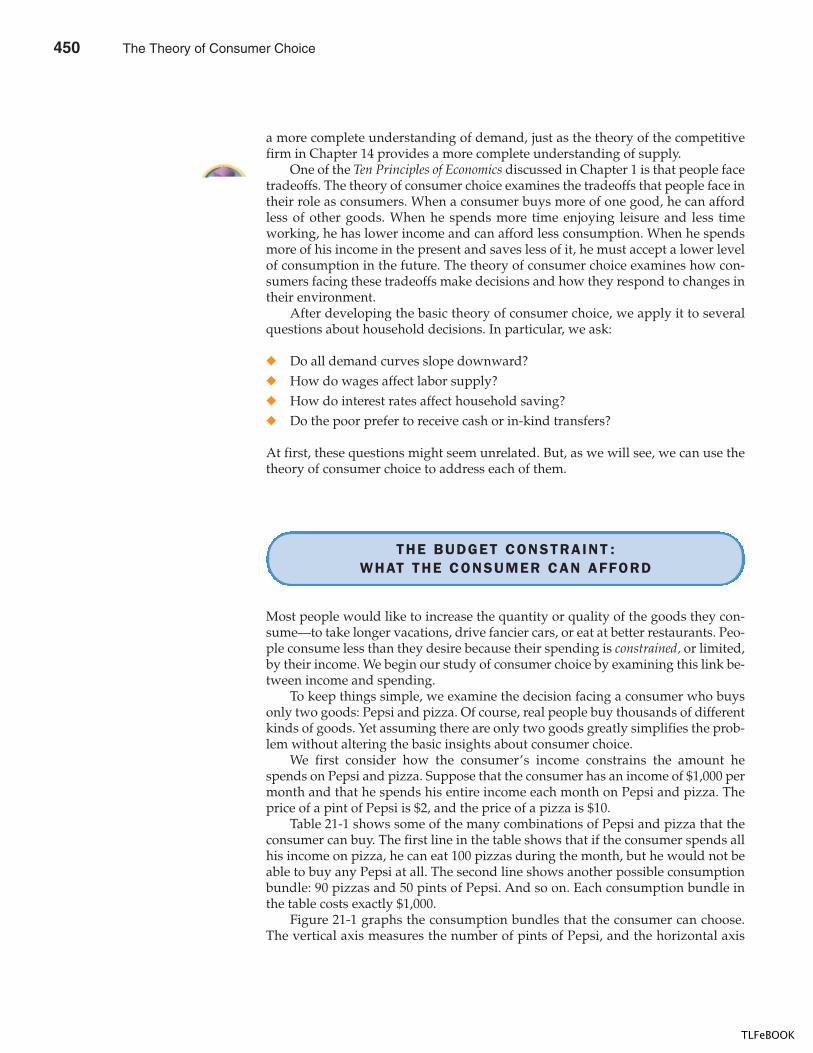
464 PART SEVEN ADVANCED TOPIC
a more complete understanding of demand, just as the theory of the competitivefirm in Chapter 14 provides a more complete understanding of supply.
One of the Ten Principles of Economics discussed in Chapter 1 is that people facetradeoffs. The theory of consumer choice examines the tradeoffs that people face intheir role as consumers. When a consumer buys more of one good, he can affordless of other goods. When he spends more time enjoying leisure and less timeworking, he has lower income and can afford less consumption. When he spendsmore of his income in the present and saves less of it, he must accept a lower levelof consumption in the future. The theory of consumer choice examines how con-sumers facing these tradeoffs make decisions and how they respond to changes intheir environment.
After developing the basic theory of consumer choice, we apply it to severalquestions about household decisions. In particular, we ask:
� Do all demand curves slope downward?� How do wages affect labor supply?� How do interest rates affect household saving?� Do the poor prefer to receive cash or in-kind transfers?
At first, these questions might seem unrelated. But, as we will see, we can use thetheory of consumer choice to address each of them.
THE BUDGET CONSTRAINT :WHAT THE CONSUMER CAN AFFORD
Most people would like to increase the quantity or quality of the goods they con-sume—to take longer vacations, drive fancier cars, or eat at better restaurants. Peo-ple consume less than they desire because their spending is constrained, or limited,by their income. We begin our study of consumer choice by examining this link be-tween income and spending.
To keep things simple, we examine the decision facing a consumer who buysonly two goods: Pepsi and pizza. Of course, real people buy thousands of differentkinds of goods. Yet assuming there are only two goods greatly simplifies the prob-lem without altering the basic insights about consumer choice.
We first consider how the consumer’s income constrains the amount hespends on Pepsi and pizza. Suppose that the consumer has an income of $1,000 permonth and that he spends his entire income each month on Pepsi and pizza. Theprice of a pint of Pepsi is $2, and the price of a pizza is $10.
Table 21-1 shows some of the many combinations of Pepsi and pizza that theconsumer can buy. The first line in the table shows that if the consumer spends allhis income on pizza, he can eat 100 pizzas during the month, but he would not beable to buy any Pepsi at all. The second line shows another possible consumptionbundle: 90 pizzas and 50 pints of Pepsi. And so on. Each consumption bundle inthe table costs exactly $1,000.
Figure 21-1 graphs the consumption bundles that the consumer can choose.The vertical axis measures the number of pints of Pepsi, and the horizontal axis
450 The Theory of Consumer Choice
TLFeBOOK
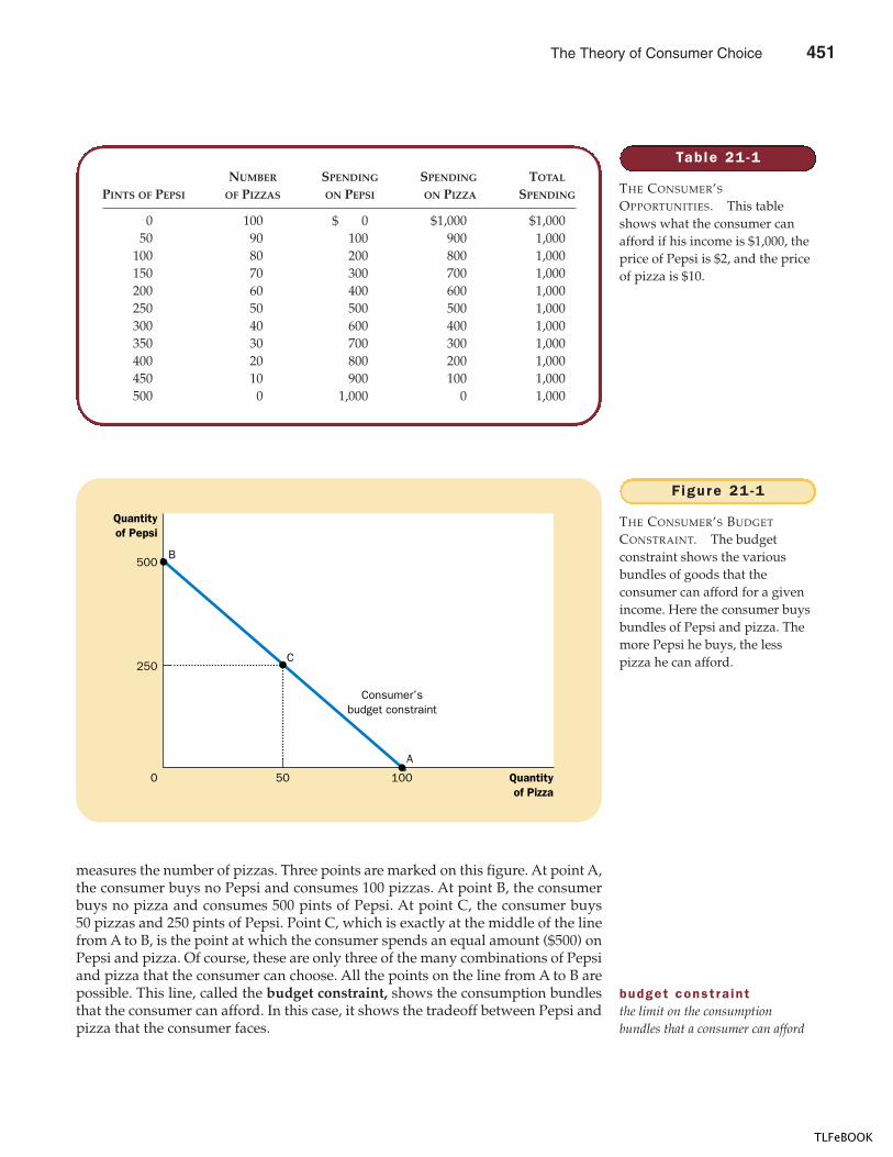
CHAPTER 21 THE THEORY OF CONSUMER CHOICE 465
measures the number of pizzas. Three points are marked on this figure. At point A,the consumer buys no Pepsi and consumes 100 pizzas. At point B, the consumerbuys no pizza and consumes 500 pints of Pepsi. At point C, the consumer buys50 pizzas and 250 pints of Pepsi. Point C, which is exactly at the middle of the linefrom A to B, is the point at which the consumer spends an equal amount ($500) onPepsi and pizza. Of course, these are only three of the many combinations of Pepsiand pizza that the consumer can choose. All the points on the line from A to B arepossible. This line, called the budget constraint, shows the consumption bundlesthat the consumer can afford. In this case, it shows the tradeoff between Pepsi andpizza that the consumer faces.
Table 21 -1
THE CONSUMER’S
OPPORTUNITIES. This tableshows what the consumer canafford if his income is $1,000, theprice of Pepsi is $2, and the priceof pizza is $10.
NUMBER SPENDING SPENDING TOTAL
PINTS OF PEPSI OF PIZZAS ON PEPSI ON PIZZA SPENDING
0 100 $ 0 $1,000 $1,00050 90 100 900 1,000
100 80 200 800 1,000150 70 300 700 1,000200 60 400 600 1,000250 50 500 500 1,000300 40 600 400 1,000350 30 700 300 1,000400 20 800 200 1,000450 10 900 100 1,000500 0 1,000 0 1,000
100 Quantityof Pizza
Quantityof Pepsi
0
250
50
500B
C
A
Consumer’sbudget constraint
Figure 21 -1
THE CONSUMER’S BUDGET
CONSTRAINT. The budgetconstraint shows the variousbundles of goods that theconsumer can afford for a givenincome. Here the consumer buysbundles of Pepsi and pizza. Themore Pepsi he buys, the lesspizza he can afford.
budget const ra intthe limit on the consumptionbundles that a consumer can afford
The Theory of Consumer Choice 451
TLFeBOOK
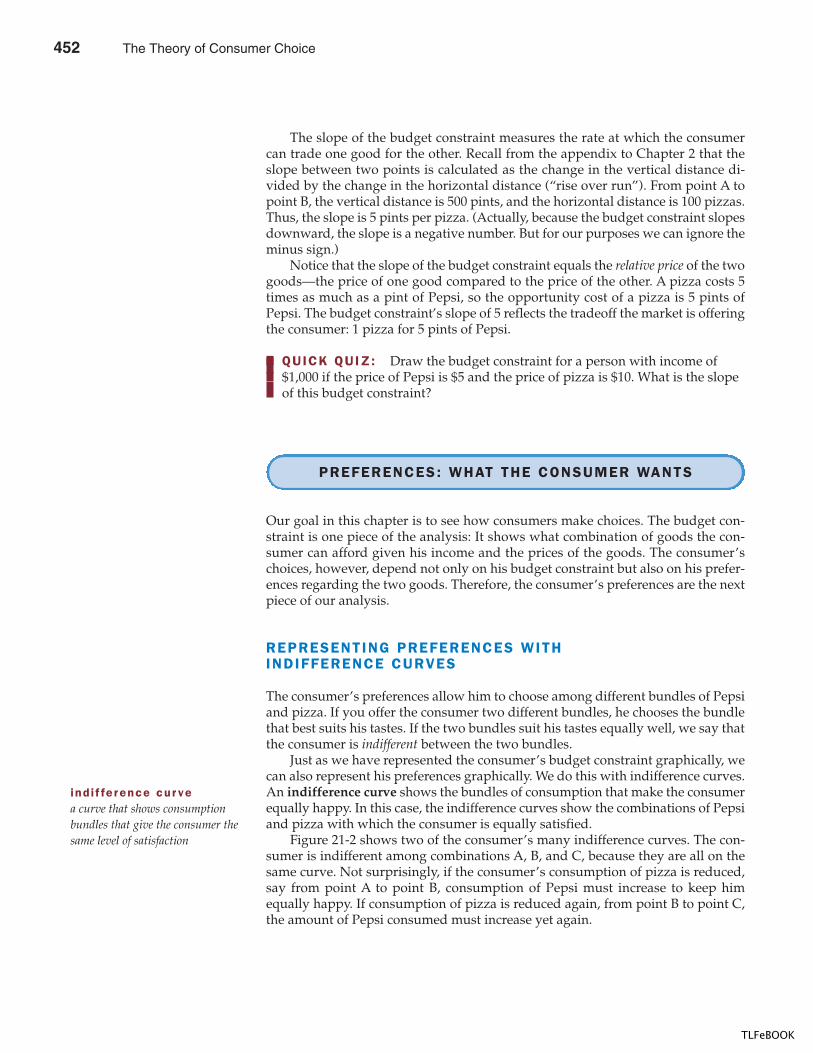
466 PART SEVEN ADVANCED TOPIC
The slope of the budget constraint measures the rate at which the consumercan trade one good for the other. Recall from the appendix to Chapter 2 that theslope between two points is calculated as the change in the vertical distance di-vided by the change in the horizontal distance (“rise over run”). From point A topoint B, the vertical distance is 500 pints, and the horizontal distance is 100 pizzas.Thus, the slope is 5 pints per pizza. (Actually, because the budget constraint slopesdownward, the slope is a negative number. But for our purposes we can ignore theminus sign.)
Notice that the slope of the budget constraint equals the relative price of the twogoods—the price of one good compared to the price of the other. A pizza costs 5times as much as a pint of Pepsi, so the opportunity cost of a pizza is 5 pints ofPepsi. The budget constraint’s slope of 5 reflects the tradeoff the market is offeringthe consumer: 1 pizza for 5 pints of Pepsi.
QUICK QUIZ: Draw the budget constraint for a person with income of $1,000 if the price of Pepsi is $5 and the price of pizza is $10. What is the slope of this budget constraint?
PREFERENCES: WHAT THE CONSUMER WANTS
Our goal in this chapter is to see how consumers make choices. The budget con-straint is one piece of the analysis: It shows what combination of goods the con-sumer can afford given his income and the prices of the goods. The consumer’schoices, however, depend not only on his budget constraint but also on his prefer-ences regarding the two goods. Therefore, the consumer’s preferences are the nextpiece of our analysis.
REPRESENTING PREFERENCES WITHINDIFFERENCE CURVES
The consumer’s preferences allow him to choose among different bundles of Pepsiand pizza. If you offer the consumer two different bundles, he chooses the bundlethat best suits his tastes. If the two bundles suit his tastes equally well, we say thatthe consumer is indifferent between the two bundles.
Just as we have represented the consumer’s budget constraint graphically, wecan also represent his preferences graphically. We do this with indifference curves.An indifference curve shows the bundles of consumption that make the consumerequally happy. In this case, the indifference curves show the combinations of Pepsiand pizza with which the consumer is equally satisfied.
Figure 21-2 shows two of the consumer’s many indifference curves. The con-sumer is indifferent among combinations A, B, and C, because they are all on thesame curve. Not surprisingly, if the consumer’s consumption of pizza is reduced,say from point A to point B, consumption of Pepsi must increase to keep himequally happy. If consumption of pizza is reduced again, from point B to point C,the amount of Pepsi consumed must increase yet again.
ind i f fe rence cur vea curve that shows consumptionbundles that give the consumer thesame level of satisfaction
452 The Theory of Consumer Choice
TLFeBOOK
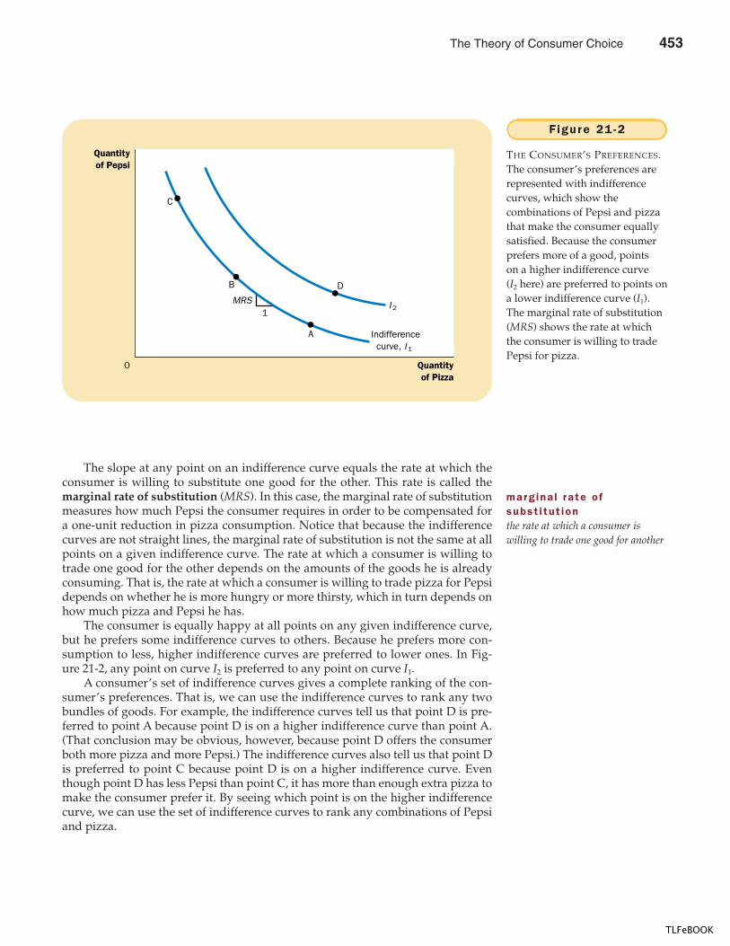
CHAPTER 21 THE THEORY OF CONSUMER CHOICE 467
The slope at any point on an indifference curve equals the rate at which theconsumer is willing to substitute one good for the other. This rate is called themarginal rate of substitution (MRS). In this case, the marginal rate of substitutionmeasures how much Pepsi the consumer requires in order to be compensated fora one-unit reduction in pizza consumption. Notice that because the indifferencecurves are not straight lines, the marginal rate of substitution is not the same at allpoints on a given indifference curve. The rate at which a consumer is willing totrade one good for the other depends on the amounts of the goods he is alreadyconsuming. That is, the rate at which a consumer is willing to trade pizza for Pepsidepends on whether he is more hungry or more thirsty, which in turn depends onhow much pizza and Pepsi he has.
The consumer is equally happy at all points on any given indifference curve,but he prefers some indifference curves to others. Because he prefers more con-sumption to less, higher indifference curves are preferred to lower ones. In Fig-ure 21-2, any point on curve I2 is preferred to any point on curve I1.
A consumer’s set of indifference curves gives a complete ranking of the con-sumer’s preferences. That is, we can use the indifference curves to rank any twobundles of goods. For example, the indifference curves tell us that point D is pre-ferred to point A because point D is on a higher indifference curve than point A.(That conclusion may be obvious, however, because point D offers the consumerboth more pizza and more Pepsi.) The indifference curves also tell us that point Dis preferred to point C because point D is on a higher indifference curve. Eventhough point D has less Pepsi than point C, it has more than enough extra pizza tomake the consumer prefer it. By seeing which point is on the higher indifferencecurve, we can use the set of indifference curves to rank any combinations of Pepsiand pizza.
Quantityof Pizza
Quantityof Pepsi
0
C
B
1
A
D
Indifferencecurve, I 1
I 2MRS
Figure 21 -2
THE CONSUMER’S PREFERENCES.The consumer’s preferences arerepresented with indifferencecurves, which show thecombinations of Pepsi and pizzathat make the consumer equallysatisfied. Because the consumerprefers more of a good, pointson a higher indifference curve(I2 here) are preferred to points ona lower indifference curve (I1).The marginal rate of substitution(MRS) shows the rate at whichthe consumer is willing to tradePepsi for pizza.
marg ina l rate o fsubst i tut ionthe rate at which a consumer iswilling to trade one good for another
The Theory of Consumer Choice 453
TLFeBOOK
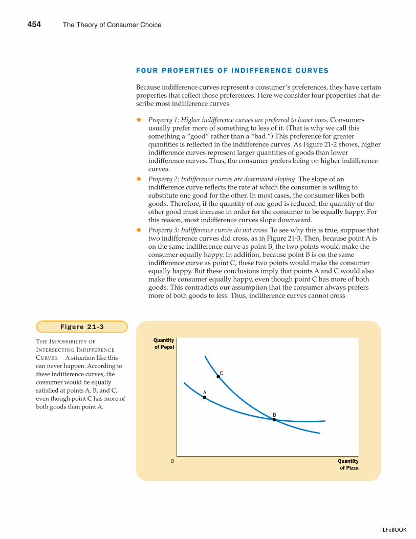
468 PART SEVEN ADVANCED TOPIC
FOUR PROPERTIES OF INDIFFERENCE CURVES
Because indifference curves represent a consumer’s preferences, they have certainproperties that reflect those preferences. Here we consider four properties that de-scribe most indifference curves:
� Property 1: Higher indifference curves are preferred to lower ones. Consumersusually prefer more of something to less of it. (That is why we call thissomething a “good” rather than a “bad.”) This preference for greaterquantities is reflected in the indifference curves. As Figure 21-2 shows, higherindifference curves represent larger quantities of goods than lowerindifference curves. Thus, the consumer prefers being on higher indifferencecurves.
� Property 2: Indifference curves are downward sloping. The slope of anindifference curve reflects the rate at which the consumer is willing tosubstitute one good for the other. In most cases, the consumer likes bothgoods. Therefore, if the quantity of one good is reduced, the quantity of theother good must increase in order for the consumer to be equally happy. Forthis reason, most indifference curves slope downward.
� Property 3: Indifference curves do not cross. To see why this is true, suppose thattwo indifference curves did cross, as in Figure 21-3. Then, because point A ison the same indifference curve as point B, the two points would make theconsumer equally happy. In addition, because point B is on the sameindifference curve as point C, these two points would make the consumerequally happy. But these conclusions imply that points A and C would alsomake the consumer equally happy, even though point C has more of bothgoods. This contradicts our assumption that the consumer always prefersmore of both goods to less. Thus, indifference curves cannot cross.
Quantityof Pizza
Quantityof Pepsi
0
C
A
B
Figure 21 -3
THE IMPOSSIBILITY OF
INTERSECTING INDIFFERENCE
CURVES. A situation like thiscan never happen. According tothese indifference curves, theconsumer would be equallysatisfied at points A, B, and C,even though point C has more ofboth goods than point A.
454 The Theory of Consumer Choice
TLFeBOOK
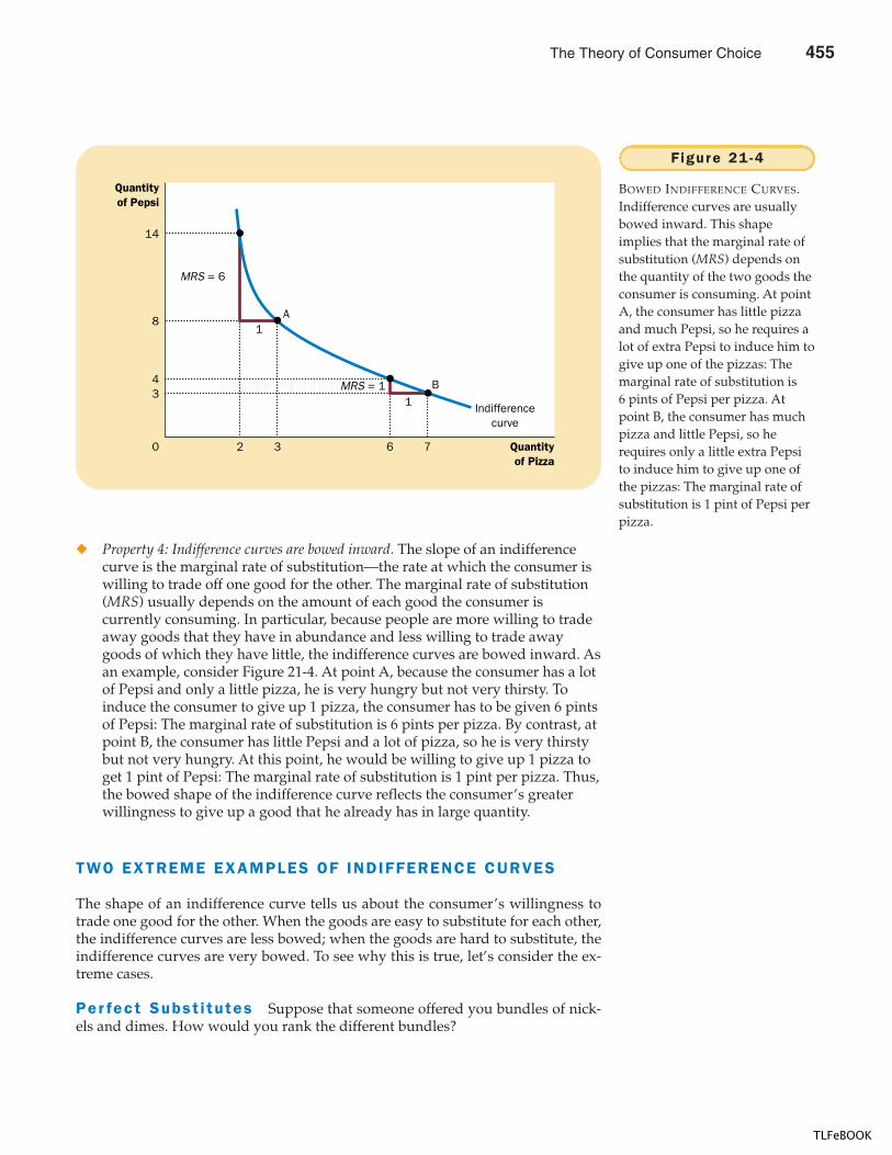
CHAPTER 21 THE THEORY OF CONSUMER CHOICE 469
� Property 4: Indifference curves are bowed inward. The slope of an indifferencecurve is the marginal rate of substitution—the rate at which the consumer iswilling to trade off one good for the other. The marginal rate of substitution(MRS) usually depends on the amount of each good the consumer iscurrently consuming. In particular, because people are more willing to tradeaway goods that they have in abundance and less willing to trade awaygoods of which they have little, the indifference curves are bowed inward. Asan example, consider Figure 21-4. At point A, because the consumer has a lotof Pepsi and only a little pizza, he is very hungry but not very thirsty. Toinduce the consumer to give up 1 pizza, the consumer has to be given 6 pintsof Pepsi: The marginal rate of substitution is 6 pints per pizza. By contrast, atpoint B, the consumer has little Pepsi and a lot of pizza, so he is very thirstybut not very hungry. At this point, he would be willing to give up 1 pizza toget 1 pint of Pepsi: The marginal rate of substitution is 1 pint per pizza. Thus,the bowed shape of the indifference curve reflects the consumer’s greaterwillingness to give up a good that he already has in large quantity.
TWO EXTREME EXAMPLES OF INDIFFERENCE CURVES
The shape of an indifference curve tells us about the consumer’s willingness totrade one good for the other. When the goods are easy to substitute for each other,the indifference curves are less bowed; when the goods are hard to substitute, theindifference curves are very bowed. To see why this is true, let’s consider the ex-treme cases.
Per fect Subst i tutes Suppose that someone offered you bundles of nick-els and dimes. How would you rank the different bundles?
Quantityof Pizza
Quantityof Pepsi
14
8
43
0 2 3 6 7
Indifferencecurve
1
1
A
B
MRS = 6
MRS = 1
Figure 21 -4
BOWED INDIFFERENCE CURVES.Indifference curves are usuallybowed inward. This shapeimplies that the marginal rate ofsubstitution (MRS) depends onthe quantity of the two goods theconsumer is consuming. At pointA, the consumer has little pizzaand much Pepsi, so he requires alot of extra Pepsi to induce him togive up one of the pizzas: Themarginal rate of substitution is6 pints of Pepsi per pizza. Atpoint B, the consumer has muchpizza and little Pepsi, so herequires only a little extra Pepsito induce him to give up one ofthe pizzas: The marginal rate ofsubstitution is 1 pint of Pepsi perpizza.
The Theory of Consumer Choice 455
TLFeBOOK
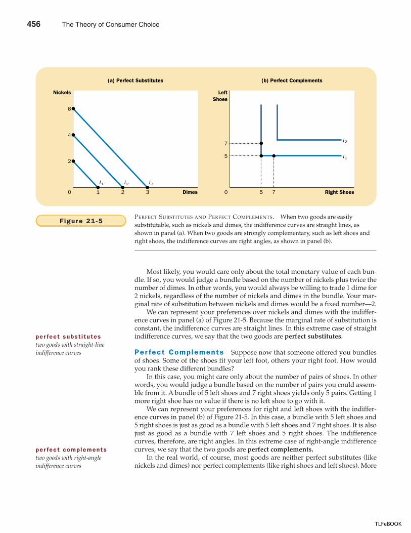
470 PART SEVEN ADVANCED TOPIC
Most likely, you would care only about the total monetary value of each bun-dle. If so, you would judge a bundle based on the number of nickels plus twice thenumber of dimes. In other words, you would always be willing to trade 1 dime for2 nickels, regardless of the number of nickels and dimes in the bundle. Your mar-ginal rate of substitution between nickels and dimes would be a fixed number—2.
We can represent your preferences over nickels and dimes with the indiffer-ence curves in panel (a) of Figure 21-5. Because the marginal rate of substitution isconstant, the indifference curves are straight lines. In this extreme case of straightindifference curves, we say that the two goods are perfect substitutes.
Per fect Complements Suppose now that someone offered you bundlesof shoes. Some of the shoes fit your left foot, others your right foot. How wouldyou rank these different bundles?
In this case, you might care only about the number of pairs of shoes. In otherwords, you would judge a bundle based on the number of pairs you could assem-ble from it. A bundle of 5 left shoes and 7 right shoes yields only 5 pairs. Getting 1more right shoe has no value if there is no left shoe to go with it.
We can represent your preferences for right and left shoes with the indiffer-ence curves in panel (b) of Figure 21-5. In this case, a bundle with 5 left shoes and5 right shoes is just as good as a bundle with 5 left shoes and 7 right shoes. It is alsojust as good as a bundle with 7 left shoes and 5 right shoes. The indifferencecurves, therefore, are right angles. In this extreme case of right-angle indifferencecurves, we say that the two goods are perfect complements.
In the real world, of course, most goods are neither perfect substitutes (likenickels and dimes) nor perfect complements (like right shoes and left shoes). More
Dimes1 2 3 750
Nickels
6
4
2
(a) Perfect Substitutes
Right Shoes0
LeftShoes
7
5
(b) Perfect Complements
I 1 I 2 I 3
I 1
I 2
Figure 21 -5PERFECT SUBSTITUTES AND PERFECT COMPLEMENTS. When two goods are easilysubstitutable, such as nickels and dimes, the indifference curves are straight lines, asshown in panel (a). When two goods are strongly complementary, such as left shoes andright shoes, the indifference curves are right angles, as shown in panel (b).
per fect subst i tutestwo goods with straight-lineindifference curves
per fect complementstwo goods with right-angleindifference curves
456 The Theory of Consumer Choice
TLFeBOOK
CHAPTER 21 THE THEORY OF CONSUMER CHOICE 471
typically, the indifference curves are bowed inward, but not so bowed as to be-come right angles.
QUICK QUIZ: Draw some indifference curves for Pepsi and pizza. Explain the four properties of these indifference curves.
OPTIMIZATION: WHAT THE CONSUMER CHOOSES
The goal of this chapter is to understand how a consumer makes choices. We havethe two pieces necessary for this analysis: the consumer’s budget constraint andthe consumer’s preferences. Now we put these two pieces together and considerthe consumer’s decision about what to buy.
THE CONSUMER’S OPTIMAL CHOICES
Consider once again our Pepsi and pizza example. The consumer would like toend up with the best possible combination of Pepsi and pizza—that is, the combi-nation on the highest possible indifference curve. But the consumer must also endup on or below his budget constraint, which measures the total resources availableto him.
Figure 21-6 shows the consumer’s budget constraint and three of his many in-difference curves. The highest indifference curve that the consumer can reach (I2 inthe figure) is the one that just barely touches the budget constraint. The point atwhich this indifference curve and the budget constraint touch is called the opti-mum. The consumer would prefer point A, but he cannot afford that point because
We have used indifferencecurves to represent the con-sumer’s preferences. Anothercommon way to represent pref-erences is with the concept ofutility. Utility is an abstract mea-sure of the satisfaction or happi-ness that a consumer receivesfrom a bundle of goods. Econo-mists say that a consumerprefers one bundle of goods toanother if the first providesmore utility than the second.
Indifference curves and utility are closely related. Be-cause the consumer prefers points on higher indifference
curves, bundles of goods on higher indifference curves pro-vide higher utility. Because the consumer is equally happywith all points on the same indifference curve, all thesebundles provide the same utility. Indeed, you can think of anindifference curve as an “equal-utility” curve. The slope ofthe indifference curve (the marginal rate of substitution) re-flects the marginal utility generated by one good comparedto the marginal utility generated by the other good.
When economists discuss the theory of consumerchoice, they might express the theory using different words.One economist might say that the goal of the consumer is tomaximize utility. Another might say that the goal of the con-sumer is to end up on the highest possible indifferencecurve. In essence, these are two ways of saying the samething.
FYIUtility: AnAlternative
Way toRepresent aConsumer’sPreferences
The Theory of Consumer Choice 457
TLFeBOOK
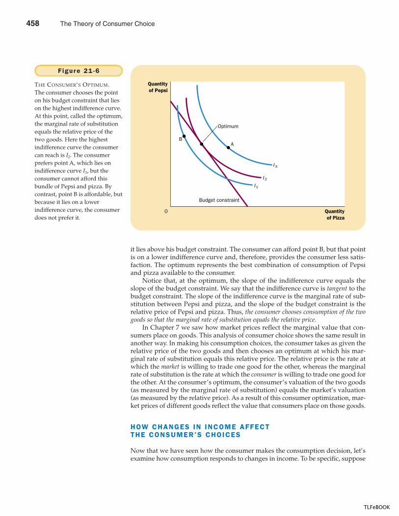
472 PART SEVEN ADVANCED TOPIC
it lies above his budget constraint. The consumer can afford point B, but that pointis on a lower indifference curve and, therefore, provides the consumer less satis-faction. The optimum represents the best combination of consumption of Pepsiand pizza available to the consumer.
Notice that, at the optimum, the slope of the indifference curve equals theslope of the budget constraint. We say that the indifference curve is tangent to thebudget constraint. The slope of the indifference curve is the marginal rate of sub-stitution between Pepsi and pizza, and the slope of the budget constraint is therelative price of Pepsi and pizza. Thus, the consumer chooses consumption of the twogoods so that the marginal rate of substitution equals the relative price.
In Chapter 7 we saw how market prices reflect the marginal value that con-sumers place on goods. This analysis of consumer choice shows the same result inanother way. In making his consumption choices, the consumer takes as given therelative price of the two goods and then chooses an optimum at which his mar-ginal rate of substitution equals this relative price. The relative price is the rate atwhich the market is willing to trade one good for the other, whereas the marginalrate of substitution is the rate at which the consumer is willing to trade one good forthe other. At the consumer’s optimum, the consumer’s valuation of the two goods(as measured by the marginal rate of substitution) equals the market’s valuation(as measured by the relative price). As a result of this consumer optimization, mar-ket prices of different goods reflect the value that consumers place on those goods.
HOW CHANGES IN INCOME AFFECTTHE CONSUMER’S CHOICES
Now that we have seen how the consumer makes the consumption decision, let’sexamine how consumption responds to changes in income. To be specific, suppose
Quantityof Pizza
Quantityof Pepsi
0
Optimum
AB
Budget constraint
I 1
I 2
I 3
Figure 21 -6
THE CONSUMER’S OPTIMUM.The consumer chooses the pointon his budget constraint that lieson the highest indifference curve.At this point, called the optimum,the marginal rate of substitutionequals the relative price of thetwo goods. Here the highestindifference curve the consumercan reach is I2. The consumerprefers point A, which lies onindifference curve I3, but theconsumer cannot afford thisbundle of Pepsi and pizza. Bycontrast, point B is affordable, butbecause it lies on a lowerindifference curve, the consumerdoes not prefer it.
458 The Theory of Consumer Choice
TLFeBOOK
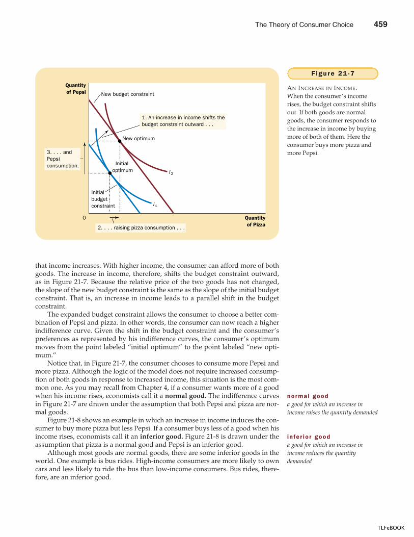
CHAPTER 21 THE THEORY OF CONSUMER CHOICE 473
that income increases. With higher income, the consumer can afford more of bothgoods. The increase in income, therefore, shifts the budget constraint outward,as in Figure 21-7. Because the relative price of the two goods has not changed,the slope of the new budget constraint is the same as the slope of the initial budgetconstraint. That is, an increase in income leads to a parallel shift in the budgetconstraint.
The expanded budget constraint allows the consumer to choose a better com-bination of Pepsi and pizza. In other words, the consumer can now reach a higherindifference curve. Given the shift in the budget constraint and the consumer’spreferences as represented by his indifference curves, the consumer’s optimummoves from the point labeled “initial optimum” to the point labeled “new opti-mum.”
Notice that, in Figure 21-7, the consumer chooses to consume more Pepsi andmore pizza. Although the logic of the model does not require increased consump-tion of both goods in response to increased income, this situation is the most com-mon one. As you may recall from Chapter 4, if a consumer wants more of a goodwhen his income rises, economists call it a normal good. The indifference curvesin Figure 21-7 are drawn under the assumption that both Pepsi and pizza are nor-mal goods.
Figure 21-8 shows an example in which an increase in income induces the con-sumer to buy more pizza but less Pepsi. If a consumer buys less of a good when hisincome rises, economists call it an inferior good. Figure 21-8 is drawn under theassumption that pizza is a normal good and Pepsi is an inferior good.
Although most goods are normal goods, there are some inferior goods in theworld. One example is bus rides. High-income consumers are more likely to owncars and less likely to ride the bus than low-income consumers. Bus rides, there-fore, are an inferior good.
Quantityof Pizza
Quantityof Pepsi
0
New optimum
New budget constraint
I 1
I 2
2. . . . raising pizza consumption . . .
3. . . . andPepsiconsumption.
Initialbudgetconstraint
Initialoptimum
1. An increase in income shifts thebudget constraint outward . . .
Figure 21 -7
AN INCREASE IN INCOME.When the consumer’s incomerises, the budget constraint shiftsout. If both goods are normalgoods, the consumer responds tothe increase in income by buyingmore of both of them. Here theconsumer buys more pizza andmore Pepsi.
normal gooda good for which an increase inincome raises the quantity demanded
in fe r io r gooda good for which an increase inincome reduces the quantitydemanded
The Theory of Consumer Choice 459
TLFeBOOK
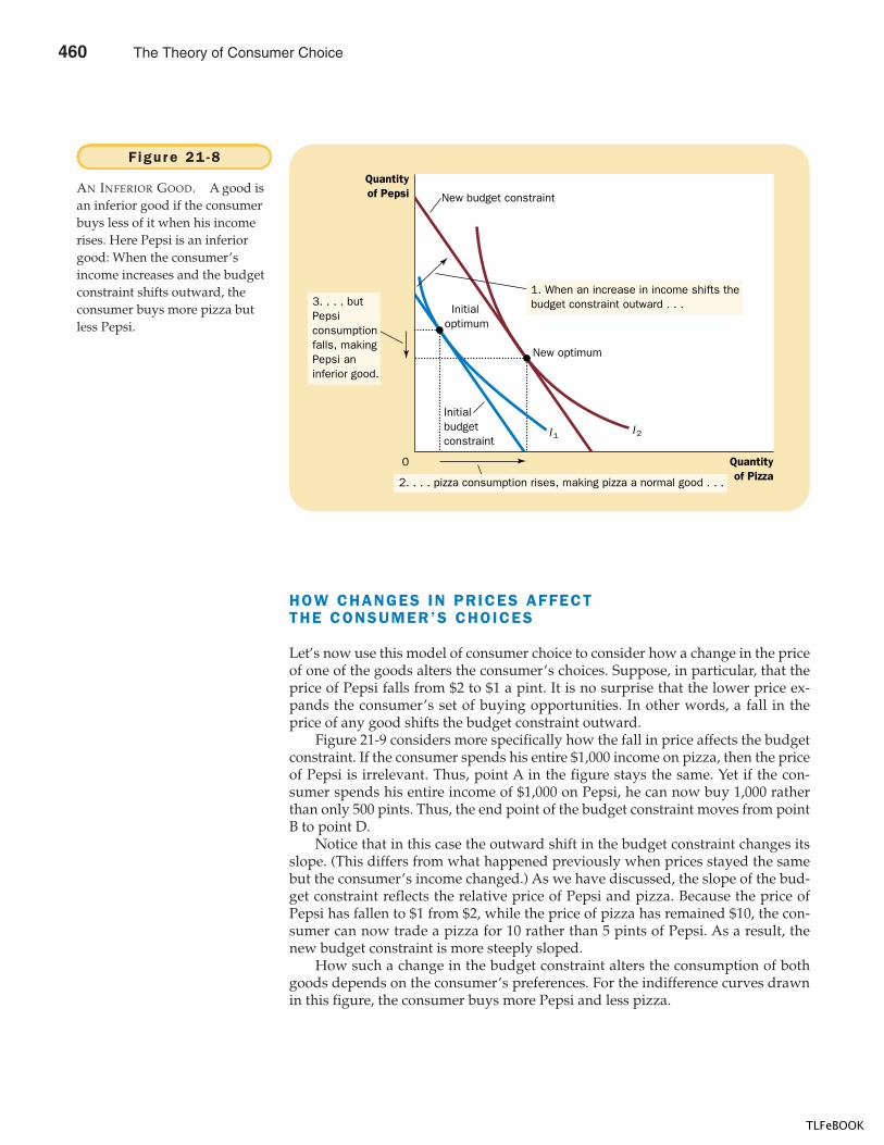
474 PART SEVEN ADVANCED TOPIC
HOW CHANGES IN PRICES AFFECTTHE CONSUMER’S CHOICES
Let’s now use this model of consumer choice to consider how a change in the priceof one of the goods alters the consumer’s choices. Suppose, in particular, that theprice of Pepsi falls from $2 to $1 a pint. It is no surprise that the lower price ex-pands the consumer’s set of buying opportunities. In other words, a fall in theprice of any good shifts the budget constraint outward.
Figure 21-9 considers more specifically how the fall in price affects the budgetconstraint. If the consumer spends his entire $1,000 income on pizza, then the priceof Pepsi is irrelevant. Thus, point A in the figure stays the same. Yet if the con-sumer spends his entire income of $1,000 on Pepsi, he can now buy 1,000 ratherthan only 500 pints. Thus, the end point of the budget constraint moves from pointB to point D.
Notice that in this case the outward shift in the budget constraint changes itsslope. (This differs from what happened previously when prices stayed the samebut the consumer’s income changed.) As we have discussed, the slope of the bud-get constraint reflects the relative price of Pepsi and pizza. Because the price ofPepsi has fallen to $1 from $2, while the price of pizza has remained $10, the con-sumer can now trade a pizza for 10 rather than 5 pints of Pepsi. As a result, thenew budget constraint is more steeply sloped.
How such a change in the budget constraint alters the consumption of bothgoods depends on the consumer’s preferences. For the indifference curves drawnin this figure, the consumer buys more Pepsi and less pizza.
Quantityof Pizza
Quantityof Pepsi
0
Initialoptimum
New optimum
Initialbudgetconstraint
New budget constraint
I 1 I 2
1. When an increase in income shifts thebudget constraint outward . . .3. . . . but
Pepsiconsumptionfalls, makingPepsi aninferior good.
2. . . . pizza consumption rises, making pizza a normal good . . .
Figure 21 -8
AN INFERIOR GOOD. A good isan inferior good if the consumerbuys less of it when his incomerises. Here Pepsi is an inferiorgood: When the consumer’sincome increases and the budgetconstraint shifts outward, theconsumer buys more pizza butless Pepsi.
460 The Theory of Consumer Choice
TLFeBOOK
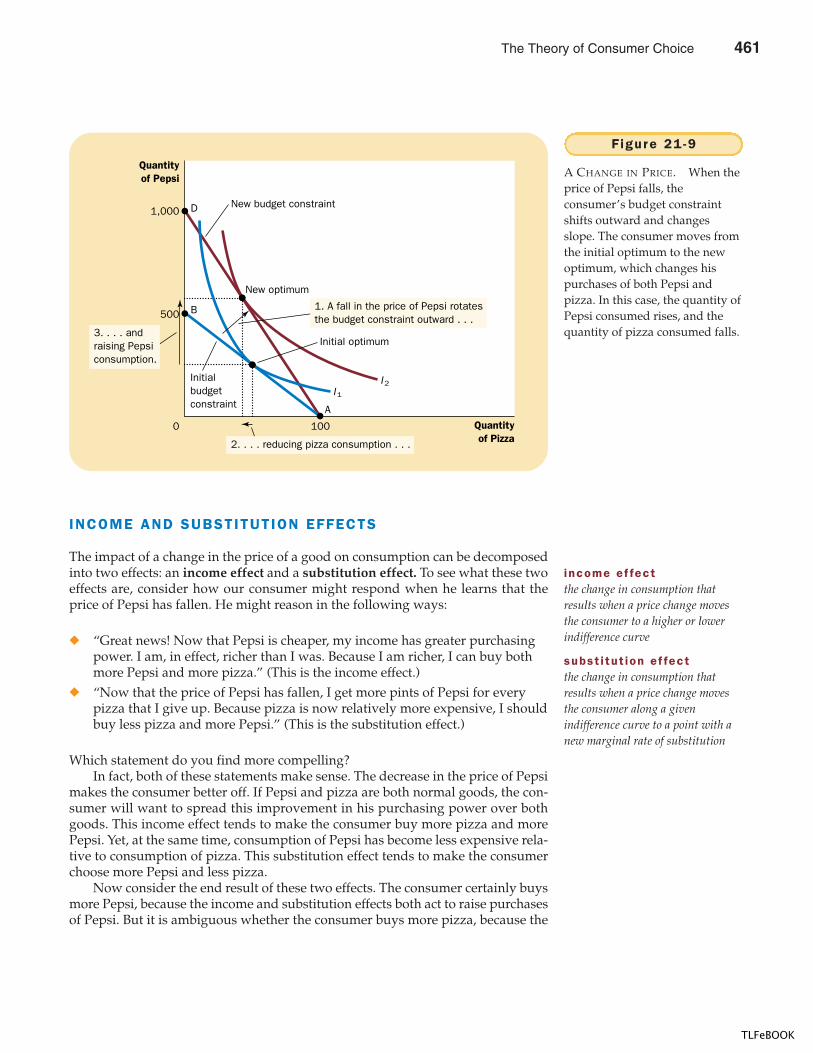
CHAPTER 21 THE THEORY OF CONSUMER CHOICE 475
INCOME AND SUBSTITUTION EFFECTS
The impact of a change in the price of a good on consumption can be decomposedinto two effects: an income effect and a substitution effect. To see what these twoeffects are, consider how our consumer might respond when he learns that theprice of Pepsi has fallen. He might reason in the following ways:
� “Great news! Now that Pepsi is cheaper, my income has greater purchasingpower. I am, in effect, richer than I was. Because I am richer, I can buy bothmore Pepsi and more pizza.” (This is the income effect.)
� “Now that the price of Pepsi has fallen, I get more pints of Pepsi for everypizza that I give up. Because pizza is now relatively more expensive, I shouldbuy less pizza and more Pepsi.” (This is the substitution effect.)
Which statement do you find more compelling?In fact, both of these statements make sense. The decrease in the price of Pepsi
makes the consumer better off. If Pepsi and pizza are both normal goods, the con-sumer will want to spread this improvement in his purchasing power over bothgoods. This income effect tends to make the consumer buy more pizza and morePepsi. Yet, at the same time, consumption of Pepsi has become less expensive rela-tive to consumption of pizza. This substitution effect tends to make the consumerchoose more Pepsi and less pizza.
Now consider the end result of these two effects. The consumer certainly buysmore Pepsi, because the income and substitution effects both act to raise purchasesof Pepsi. But it is ambiguous whether the consumer buys more pizza, because the
Quantityof Pizza
100
Quantityof Pepsi
1,000
500
0
B
D
A
New optimum
I1
I2
Initial optimum
New budget constraint
Initialbudgetconstraint
1. A fall in the price of Pepsi rotates the budget constraint outward . . .
3. . . . andraising Pepsiconsumption.
2. . . . reducing pizza consumption . . .
Figure 21 -9
A CHANGE IN PRICE. When theprice of Pepsi falls, theconsumer’s budget constraintshifts outward and changesslope. The consumer moves fromthe initial optimum to the newoptimum, which changes hispurchases of both Pepsi andpizza. In this case, the quantity ofPepsi consumed rises, and thequantity of pizza consumed falls.
income e f fectthe change in consumption thatresults when a price change movesthe consumer to a higher or lowerindifference curve
subst i tut ion e f fectthe change in consumption thatresults when a price change movesthe consumer along a givenindifference curve to a point with anew marginal rate of substitution
The Theory of Consumer Choice 461
TLFeBOOK
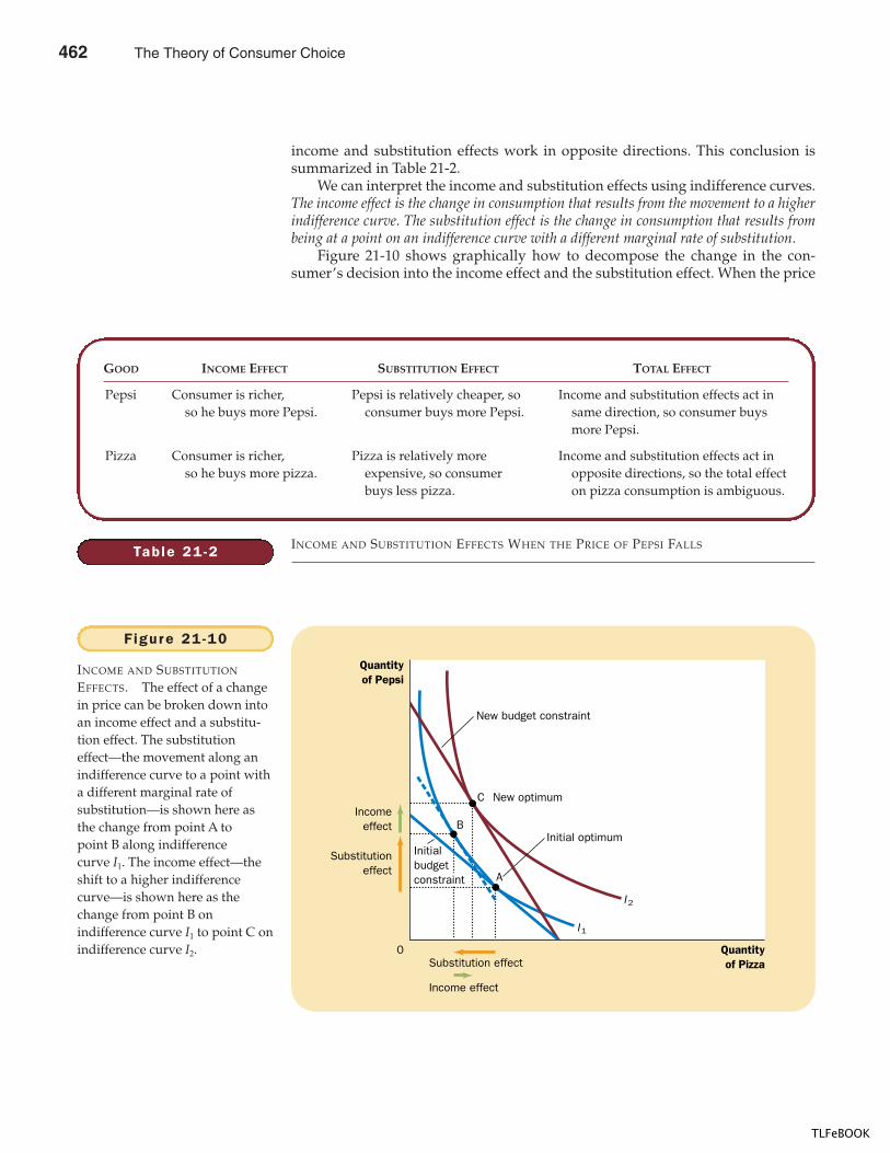
476 PART SEVEN ADVANCED TOPIC
income and substitution effects work in opposite directions. This conclusion issummarized in Table 21-2.
We can interpret the income and substitution effects using indifference curves.The income effect is the change in consumption that results from the movement to a higherindifference curve. The substitution effect is the change in consumption that results frombeing at a point on an indifference curve with a different marginal rate of substitution.
Figure 21-10 shows graphically how to decompose the change in the con-sumer’s decision into the income effect and the substitution effect. When the price
Table 21 -2
GOOD INCOME EFFECT SUBSTITUTION EFFECT TOTAL EFFECT
Pepsi Consumer is richer, Pepsi is relatively cheaper, so Income and substitution effects act in so he buys more Pepsi. consumer buys more Pepsi. same direction, so consumer buys
more Pepsi.
Pizza Consumer is richer, Pizza is relatively more Income and substitution effects act in so he buys more pizza. expensive, so consumer opposite directions, so the total effect
buys less pizza. on pizza consumption is ambiguous.
INCOME AND SUBSTITUTION EFFECTS WHEN THE PRICE OF PEPSI FALLS
Quantityof Pizza
Quantityof Pepsi
0
Incomeeffect
Substitutioneffect
B
A
C New optimum
I1
I2
Initial optimum
New budget constraint
Initialbudgetconstraint
Substitution effect
Income effect
Figure 21 -10
INCOME AND SUBSTITUTION
EFFECTS. The effect of a changein price can be broken down intoan income effect and a substitu-tion effect. The substitutioneffect—the movement along anindifference curve to a point witha different marginal rate ofsubstitution—is shown here asthe change from point A topoint B along indifferencecurve I1. The income effect—theshift to a higher indifferencecurve—is shown here as thechange from point B onindifference curve I1 to point C onindifference curve I2.
462 The Theory of Consumer Choice
TLFeBOOK
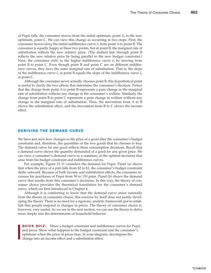
CHAPTER 21 THE THEORY OF CONSUMER CHOICE 477
of Pepsi falls, the consumer moves from the initial optimum, point A, to the newoptimum, point C. We can view this change as occurring in two steps. First, theconsumer moves along the initial indifference curve I1 from point A to point B. Theconsumer is equally happy at these two points, but at point B, the marginal rate ofsubstitution reflects the new relative price. (The dashed line through point Breflects the new relative price by being parallel to the new budget constraint.)Next, the consumer shifts to the higher indifference curve I2 by moving frompoint B to point C. Even though point B and point C are on different indiffer-ence curves, they have the same marginal rate of substitution. That is, the slopeof the indifference curve I1 at point B equals the slope of the indifference curve I2
at point C.Although the consumer never actually chooses point B, this hypothetical point
is useful to clarify the two effects that determine the consumer’s decision. Noticethat the change from point A to point B represents a pure change in the marginalrate of substitution without any change in the consumer’s welfare. Similarly, thechange from point B to point C represents a pure change in welfare without anychange in the marginal rate of substitution. Thus, the movement from A to Bshows the substitution effect, and the movement from B to C shows the incomeeffect.
DERIVING THE DEMAND CURVE
We have just seen how changes in the price of a good alter the consumer’s budgetconstraint and, therefore, the quantities of the two goods that he chooses to buy.The demand curve for any good reflects these consumption decisions. Recall thata demand curve shows the quantity demanded of a good for any given price. Wecan view a consumer’s demand curve as a summary of the optimal decisions thatarise from his budget constraint and indifference curves.
For example, Figure 21-11 considers the demand for Pepsi. Panel (a) showsthat when the price of a pint falls from $2 to $1, the consumer’s budget constraintshifts outward. Because of both income and substitution effects, the consumer in-creases his purchases of Pepsi from 50 to 150 pints. Panel (b) shows the demandcurve that results from this consumer’s decisions. In this way, the theory of con-sumer choice provides the theoretical foundation for the consumer’s demandcurve, which we first introduced in Chapter 4.
Although it is comforting to know that the demand curve arises naturallyfrom the theory of consumer choice, this exercise by itself does not justify devel-oping the theory. There is no need for a rigorous, analytic framework just to estab-lish that people respond to changes in prices. The theory of consumer choice is,however, very useful. As we see in the next section, we can use the theory to delvemore deeply into the determinants of household behavior.
QUICK QUIZ: Draw a budget constraint and indifference curves for Pepsi and pizza. Show what happens to the budget constraint and the consumer’s optimum when the price of pizza rises. In your diagram, decompose the change into an income effect and a substitution effect.
The Theory of Consumer Choice 463
TLFeBOOK
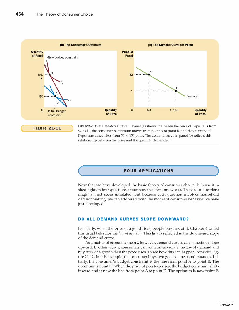
478 PART SEVEN ADVANCED TOPIC
FOUR APPLICATIONS
Now that we have developed the basic theory of consumer choice, let’s use it toshed light on four questions about how the economy works. These four questionsmight at first seem unrelated. But because each question involves householddecisionmaking, we can address it with the model of consumer behavior we havejust developed.
DO ALL DEMAND CURVES SLOPE DOWNWARD?
Normally, when the price of a good rises, people buy less of it. Chapter 4 calledthis usual behavior the law of demand. This law is reflected in the downward slopeof the demand curve.
As a matter of economic theory, however, demand curves can sometimes slopeupward. In other words, consumers can sometimes violate the law of demand andbuy more of a good when the price rises. To see how this can happen, consider Fig-ure 21-12. In this example, the consumer buys two goods—meat and potatoes. Ini-tially, the consumer’s budget constraint is the line from point A to point B. Theoptimum is point C. When the price of potatoes rises, the budget constraint shiftsinward and is now the line from point A to point D. The optimum is now point E.
Quantityof Pizza
50 1500
50 Demand
(a) The Consumer’s Optimum
Quantityof Pepsi
0
Price ofPepsi
$2
1
(b) The Demand Curve for Pepsi
Quantityof Pepsi
150B A
B
A
I1
I 2
New budget constraint
Initial budget constraint
Figure 21 -11 DERIVING THE DEMAND CURVE. Panel (a) shows that when the price of Pepsi falls from$2 to $1, the consumer’s optimum moves from point A to point B, and the quantity ofPepsi consumed rises from 50 to 150 pints. The demand curve in panel (b) reflects thisrelationship between the price and the quantity demanded.
464 The Theory of Consumer Choice
TLFeBOOK
CHAPTER 21 THE THEORY OF CONSUMER CHOICE 479
Notice that a rise in the price of potatoes has led the consumer to buy a largerquantity of potatoes.
Why is the consumer responding in a seemingly perverse way? The reason isthat potatoes here are a strongly inferior good. When the price of potatoes rises,the consumer is poorer. The income effect makes the consumer want to buy lessmeat and more potatoes. At the same time, because the potatoes have becomemore expensive relative to meat, the substitution effect makes the consumer wantto buy more meat and less potatoes. In this particular case, however, the income ef-fect is so strong that it exceeds the substitution effect. In the end, the consumer re-sponds to the higher price of potatoes by buying less meat and more potatoes.
Economists use the term Giffen good to describe a good that violates the lawof demand. (The term is named for economist Robert Giffen, who first noted thispossibility.) In this example, potatoes are a Giffen good. Giffen goods are inferiorgoods for which the income effect dominates the substitution effect. Therefore,they have demand curves that slope upward.
Economists disagree about whether any Giffen good has ever been discovered.Some historians suggest that potatoes were in fact a Giffen good during the Irishpotato famine of the nineteenth century. Potatoes were such a large part of peo-ple’s diet that when the price of potatoes rose, it had a large income effect. Peopleresponded to their reduced living standard by cutting back on the luxury of meatand buying more of the staple food of potatoes. Thus, it is argued that a higherprice of potatoes actually raised the quantity of potatoes demanded.
Whether or not this historical account is true, it is safe to say that Giffen goodsare very rare. The theory of consumer choice does allow demand curves to slopeupward. Yet such occurrences are so unusual that the law of demand is as reliablea law as any in economics.
Quantityof Meat
A
Quantity ofPotatoes
0
E
C
I2I 1
Initial budget constraint
New budgetconstraint
D
B
2. . . . which increasespotatoconsumptionif potatoesare a Giffengood.
Optimum with lowprice of potatoes
Optimum with highprice of potatoes
1. An increase in the price ofpotatoes rotates the budgetconstraint inward . . .
Figure 21 -12
A GIFFEN GOOD. In thisexample, when the price ofpotatoes rises, the consumer’soptimum shifts from point Cto point E. In this case, theconsumer responds to a higherprice of potatoes by buying lessmeat and more potatoes.
Gi f fen gooda good for which an increase in theprice raises the quantity demanded
The Theory of Consumer Choice 465
TLFeBOOK
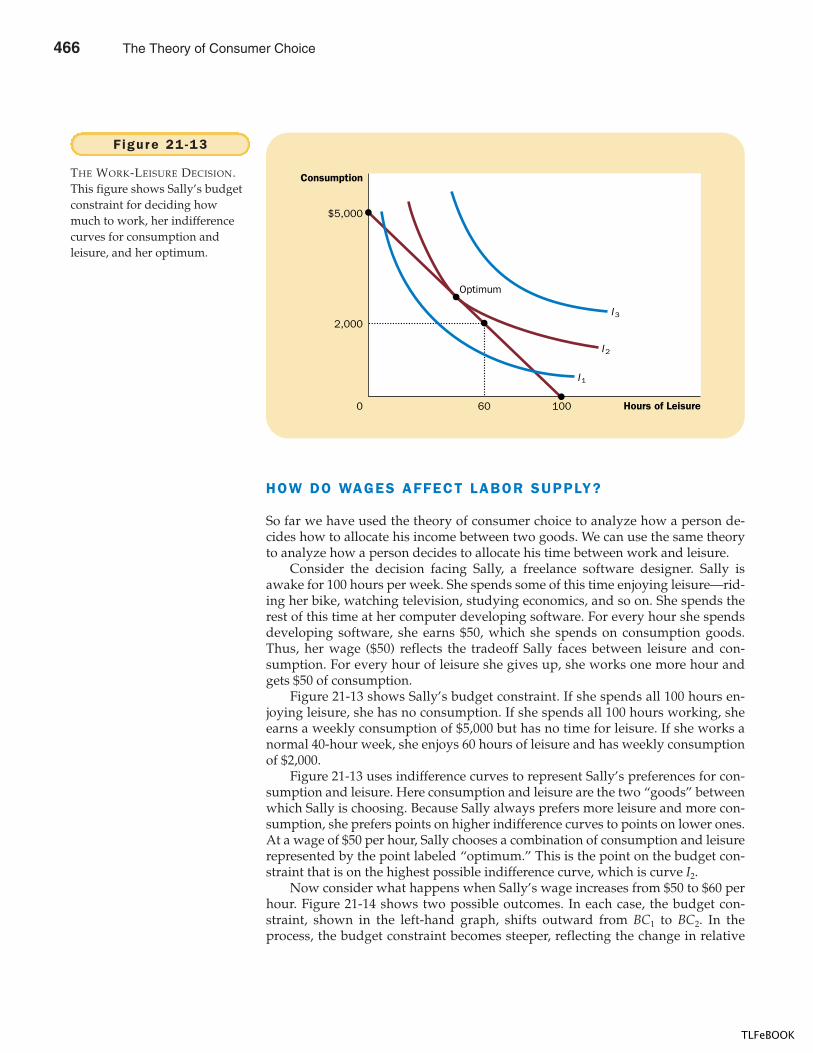
480 PART SEVEN ADVANCED TOPIC
HOW DO WAGES AFFECT LABOR SUPPLY?
So far we have used the theory of consumer choice to analyze how a person de-cides how to allocate his income between two goods. We can use the same theoryto analyze how a person decides to allocate his time between work and leisure.
Consider the decision facing Sally, a freelance software designer. Sally isawake for 100 hours per week. She spends some of this time enjoying leisure—rid-ing her bike, watching television, studying economics, and so on. She spends therest of this time at her computer developing software. For every hour she spendsdeveloping software, she earns $50, which she spends on consumption goods.Thus, her wage ($50) reflects the tradeoff Sally faces between leisure and con-sumption. For every hour of leisure she gives up, she works one more hour andgets $50 of consumption.
Figure 21-13 shows Sally’s budget constraint. If she spends all 100 hours en-joying leisure, she has no consumption. If she spends all 100 hours working, sheearns a weekly consumption of $5,000 but has no time for leisure. If she works anormal 40-hour week, she enjoys 60 hours of leisure and has weekly consumptionof $2,000.
Figure 21-13 uses indifference curves to represent Sally’s preferences for con-sumption and leisure. Here consumption and leisure are the two “goods” betweenwhich Sally is choosing. Because Sally always prefers more leisure and more con-sumption, she prefers points on higher indifference curves to points on lower ones.At a wage of $50 per hour, Sally chooses a combination of consumption and leisurerepresented by the point labeled “optimum.” This is the point on the budget con-straint that is on the highest possible indifference curve, which is curve I2.
Now consider what happens when Sally’s wage increases from $50 to $60 perhour. Figure 21-14 shows two possible outcomes. In each case, the budget con-straint, shown in the left-hand graph, shifts outward from BC1 to BC2. In theprocess, the budget constraint becomes steeper, reflecting the change in relative
Hours of Leisure0
2,000
$5,000
60
Consumption
100
Optimum
I3
I2
I 1
Figure 21 -13
THE WORK-LEISURE DECISION.This figure shows Sally’s budgetconstraint for deciding howmuch to work, her indifferencecurves for consumption andleisure, and her optimum.
466 The Theory of Consumer Choice
TLFeBOOK
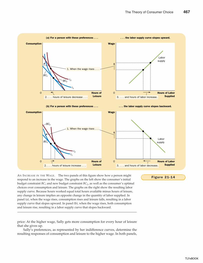
CHAPTER 21 THE THEORY OF CONSUMER CHOICE 481
price: At the higher wage, Sally gets more consumption for every hour of leisurethat she gives up.
Sally’s preferences, as represented by her indifference curves, determine theresulting responses of consumption and leisure to the higher wage. In both panels,
Hours ofLeisure
0
Consumption
(a) For a person with these preferences . . .
Hours of LaborSupplied
0
Wage
. . . the labor supply curve slopes upward.
Hours ofLeisure
0
Consumption
(b) For a person with these preferences . . .
Hours of LaborSupplied
0
Wage
. . . the labor supply curve slopes backward.
I 1
I 2BC2
BC1
I1
I 2
BC2
BC1
1. When the wage rises . . .
2. . . . hours of leisure increase . . . 3. . . . and hours of labor decrease.
2. . . . hours of leisure decrease . . . 3. . . . and hours of labor increase.
1. When the wage rises . . .
Labor supply
Labor supply
Figure 21 -14AN INCREASE IN THE WAGE. The two panels of this figure show how a person mightrespond to an increase in the wage. The graphs on the left show the consumer’s initialbudget constraint BC1 and new budget constraint BC2, as well as the consumer’s optimalchoices over consumption and leisure. The graphs on the right show the resulting laborsupply curve. Because hours worked equal total hours available minus hours of leisure,any change in leisure implies an opposite change in the quantity of labor supplied. Inpanel (a), when the wage rises, consumption rises and leisure falls, resulting in a laborsupply curve that slopes upward. In panel (b), when the wage rises, both consumptionand leisure rise, resulting in a labor supply curve that slopes backward.
The Theory of Consumer Choice 467
TLFeBOOK
482 PART SEVEN ADVANCED TOPIC
CASE STUDY INCOME EFFECTS ON LABOR SUPPLY:HISTORICAL TRENDS, LOTTERY WINNERS,AND THE CARNEGIE CONJECTURE
The idea of a backward-sloping labor supply curve might at first seem like a meretheoretical curiosity, but in fact it is not. Evidence indicates that the labor supplycurve, considered over long periods of time, does in fact slope backward. A hun-dred years ago many people worked six days a week. Today five-day workweeksare the norm. At the same time that the length of the workweek has been falling,the wage of the typical worker (adjusted for inflation) has been rising.
Here is how economists explain this historical pattern: Over time, advancesin technology raise workers’ productivity and, thereby, the demand for labor.The increase in labor demand raises equilibrium wages. As wages rise, so doesthe reward for working. Yet rather than responding to this increased incentiveby working more, most workers choose to take part of their greater prosperityin the form of more leisure. In other words, the income effect of higher wagesdominates the substitution effect.
Further evidence that the income effect on labor supply is strong comesfrom a very different kind of data: winners of lotteries. Winners of large prizes
consumption rises. Yet the response of leisure to the change in the wage is differ-ent in the two cases. In panel (a), Sally responds to the higher wage by enjoyingless leisure. In panel (b), Sally responds by enjoying more leisure.
Sally’s decision between leisure and consumption determines her supply oflabor, for the more leisure she enjoys the less time she has left to work. In eachpanel, the right-hand graph in Figure 21-14 shows the labor supply curve impliedby Sally’s decision. In panel (a), a higher wage induces Sally to enjoy less leisureand work more, so the labor supply curve slopes upward. In panel (b), a higherwage induces Sally to enjoy more leisure and work less, so the labor supply curveslopes “backward.”
At first, the backward-sloping labor supply curve is puzzling. Why would aperson respond to a higher wage by working less? The answer comes from con-sidering the income and substitution effects of a higher wage.
Consider first the substitution effect. When Sally’s wage rises, leisure becomesmore costly relative to consumption, and this encourages Sally to substitute con-sumption for leisure. In other words, the substitution effect induces Sally to workharder in response to higher wages, which tends to make the labor supply curveslope upward.
Now consider the income effect. When Sally’s wage rises, she moves to ahigher indifference curve. She is now better off than she was. As long as con-sumption and leisure are both normal goods, she tends to want to use this increasein well-being to enjoy both higher consumption and greater leisure. In otherwords, the income effect induces her to work less, which tends to make the laborsupply curve slope backward.
In the end, economic theory does not give a clear prediction about whether anincrease in the wage induces Sally to work more or less. If the substitution effect isgreater than the income effect for Sally, she works more. If the income effect isgreater than the substitution effect, she works less. The labor supply curve, there-fore, could be either upward or backward sloping.
“NO MORE 9-TO-5 FOR ME.”
468 The Theory of Consumer Choice
TLFeBOOK
CHAPTER 21 THE THEORY OF CONSUMER CHOICE 483
in the lottery see large increases in their incomes and, as a result, large outwardshifts in their budget constraints. Because the winners’ wages have notchanged, however, the slopes of their budget constraints remain the same. Thereis, therefore, no substitution effect. By examining the behavior of lottery win-ners, we can isolate the income effect on labor supply.
The results from studies of lottery winners are striking. Of those winnerswho win more than $50,000, almost 25 percent quit working within a year, andanother 9 percent reduce the number of hours they work. Of those winners whowin more than $1 million, almost 40 percent stop working. The income effect onlabor supply of winning such a large prize is substantial.
Similar results were found in a study, published in the May 1993 issue of theQuarterly Journal of Economics, of how receiving a bequest affects a person’s la-bor supply. The study found that a single person who inherits more than$150,000 is four times as likely to stop working as a single person who inheritsless than $25,000. This finding would not have surprised the nineteenth-centuryindustrialist Andrew Carnegie. Carnegie warned that “the parent who leaveshis son enormous wealth generally deadens the talents and energies of the son,and tempts him to lead a less useful and less worthy life than he otherwisewould.” That is, Carnegie viewed the income effect on labor supply to be sub-stantial and, from his paternalistic perspective, regrettable. During his life andat his death, Carnegie gave much of his vast fortune to charity.
HOW DO INTEREST RATES AFFECT HOUSEHOLD SAVING?
An important decision that every person faces is how much income to consume to-day and how much to save for the future. We can use the theory of consumerchoice to analyze how people make this decision and how the amount they savedepends on the interest rate their savings will earn.
Consider the decision facing Sam, a worker planning ahead for retirement. Tokeep things simple, let’s divide Sam’s life into two periods. In the first period, Samis young and working. In the second period, he is old and retired. When young,Sam earns a total of $100,000. He divides this income between current consump-tion and saving. When he is old, Sam will consume what he has saved, includingthe interest that his savings have earned.
Suppose that the interest rate is 10 percent. Then for every dollar that Samsaves when young, he can consume $1.10 when old. We can view “consumptionwhen young” and “consumption when old” as the two goods that Sam mustchoose between. The interest rate determines the relative price of these two goods.
Figure 21-15 shows Sam’s budget constraint. If he saves nothing, he consumes$100,000 when young and nothing when old. If he saves everything, he consumesnothing when young and $110,000 when old. The budget constraint shows theseand all the intermediate possibilities.
Figure 21-15 uses indifference curves to represent Sam’s preferences for con-sumption in the two periods. Because Sam prefers more consumption in both pe-riods, he prefers points on higher indifference curves to points on lower ones.Given his preferences, Sam chooses the optimal combination of consumption inboth periods of life, which is the point on the budget constraint that is on the high-est possible indifference curve. At this optimum, Sam consumes $50,000 whenyoung and $55,000 when old.
The Theory of Consumer Choice 469
TLFeBOOK
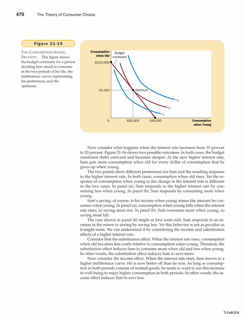
484 PART SEVEN ADVANCED TOPIC
Now consider what happens when the interest rate increases from 10 percentto 20 percent. Figure 21-16 shows two possible outcomes. In both cases, the budgetconstraint shifts outward and becomes steeper. At the new higher interest rate,Sam gets more consumption when old for every dollar of consumption that hegives up when young.
The two panels show different preferences for Sam and the resulting responseto the higher interest rate. In both cases, consumption when old rises. Yet the re-sponse of consumption when young to the change in the interest rate is differentin the two cases. In panel (a), Sam responds to the higher interest rate by con-suming less when young. In panel (b), Sam responds by consuming more whenyoung.
Sam’s saving, of course, is his income when young minus the amount he con-sumes when young. In panel (a), consumption when young falls when the interestrate rises, so saving must rise. In panel (b), Sam consumes more when young, sosaving must fall.
The case shown in panel (b) might at first seem odd: Sam responds to an in-crease in the return to saving by saving less. Yet this behavior is not as peculiar asit might seem. We can understand it by considering the income and substitutioneffects of a higher interest rate.
Consider first the substitution effect. When the interest rate rises, consumptionwhen old becomes less costly relative to consumption when young. Therefore, thesubstitution effect induces Sam to consume more when old and less when young.In other words, the substitution effect induces Sam to save more.
Now consider the income effect. When the interest rate rises, Sam moves to ahigher indifference curve. He is now better off than he was. As long as consump-tion in both periods consists of normal goods, he tends to want to use this increasein well-being to enjoy higher consumption in both periods. In other words, the in-come effect induces him to save less.
Consumptionwhen Young
0
55,000
$110,000
$50,000
Consumptionwhen Old
100,000
Optimum
I3
I2
I 1
Budgetconstraint
Figure 21 -15
THE CONSUMPTION-SAVING
DECISION. This figure showsthe budget constraint for a persondeciding how much to consumein the two periods of his life, theindifference curves representinghis preferences, and theoptimum.
470 The Theory of Consumer Choice
TLFeBOOK
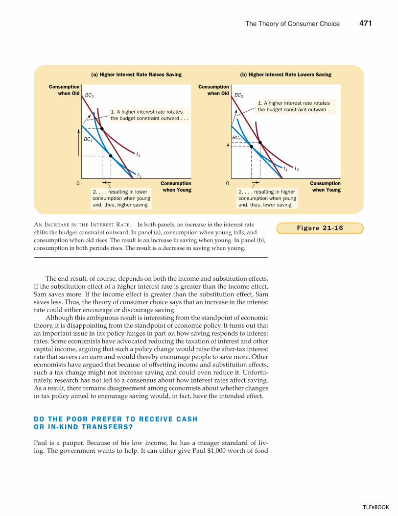
CHAPTER 21 THE THEORY OF CONSUMER CHOICE 485
The end result, of course, depends on both the income and substitution effects.If the substitution effect of a higher interest rate is greater than the income effect,Sam saves more. If the income effect is greater than the substitution effect, Samsaves less. Thus, the theory of consumer choice says that an increase in the interestrate could either encourage or discourage saving.
Although this ambiguous result is interesting from the standpoint of economictheory, it is disappointing from the standpoint of economic policy. It turns out thatan important issue in tax policy hinges in part on how saving responds to interestrates. Some economists have advocated reducing the taxation of interest and othercapital income, arguing that such a policy change would raise the after-tax interestrate that savers can earn and would thereby encourage people to save more. Othereconomists have argued that because of offsetting income and substitution effects,such a tax change might not increase saving and could even reduce it. Unfortu-nately, research has not led to a consensus about how interest rates affect saving.As a result, there remains disagreement among economists about whether changesin tax policy aimed to encourage saving would, in fact, have the intended effect.
DO THE POOR PREFER TO RECEIVE CASHOR IN-KIND TRANSFERS?
Paul is a pauper. Because of his low income, he has a meager standard of liv-ing. The government wants to help. It can either give Paul $1,000 worth of food
0
(a) Higher Interest Rate Raises Saving (b) Higher Interest Rate Lowers Saving
Consumptionwhen Old
I 1
I 2
BC1
BC2
0
I1 I 2
BC1
BC2
Consumptionwhen Old
Consumptionwhen Young
1. A higher interest rate rotatesthe budget constraint outward . . .
1. A higher interest rate rotatesthe budget constraint outward . . .
2. . . . resulting in lowerconsumption when young and, thus, higher saving.
2. . . . resulting in higherconsumption when youngand, thus, lower saving.
Consumptionwhen Young
F igure 21 -16AN INCREASE IN THE INTEREST RATE. In both panels, an increase in the interest rateshifts the budget constraint outward. In panel (a), consumption when young falls, andconsumption when old rises. The result is an increase in saving when young. In panel (b),consumption in both periods rises. The result is a decrease in saving when young.
The Theory of Consumer Choice 471
TLFeBOOK
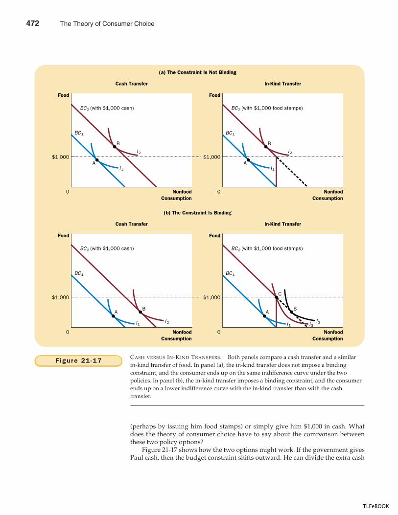
486 PART SEVEN ADVANCED TOPIC
(perhaps by issuing him food stamps) or simply give him $1,000 in cash. Whatdoes the theory of consumer choice have to say about the comparison betweenthese two policy options?
Figure 21-17 shows how the two options might work. If the government givesPaul cash, then the budget constraint shifts outward. He can divide the extra cash
Cash Transfer In-Kind Transfer
NonfoodConsumption
0
$1,000
Cash Transfer
(a) The Constraint Is Not Binding
(b) The Constraint Is Binding
0
$1,000
In-Kind Transfer
Food
AB
I2I1
BC1
BC2 (with $1,000 cash)
AB
C
I2I1
BC1
BC2 (with $1,000 food stamps)
Food
NonfoodConsumption
NonfoodConsumption
0
$1,000
0
$1,000
Food
A
B
I2
I1
BC1
BC2 (with $1,000 cash)
A
B
I2
I1
BC1
BC2 (with $1,000 food stamps)
Food
NonfoodConsumption
I3
Figure 21 -17 CASH VERSUS IN-KIND TRANSFERS. Both panels compare a cash transfer and a similarin-kind transfer of food. In panel (a), the in-kind transfer does not impose a bindingconstraint, and the consumer ends up on the same indifference curve under the twopolicies. In panel (b), the in-kind transfer imposes a binding constraint, and the consumerends up on a lower indifference curve with the in-kind transfer than with the cashtransfer.
472 The Theory of Consumer Choice
TLFeBOOK
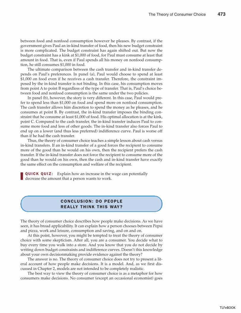
CHAPTER 21 THE THEORY OF CONSUMER CHOICE 487
between food and nonfood consumption however he pleases. By contrast, if thegovernment gives Paul an in-kind transfer of food, then his new budget constraintis more complicated. The budget constraint has again shifted out. But now thebudget constraint has a kink at $1,000 of food, for Paul must consume at least thatamount in food. That is, even if Paul spends all his money on nonfood consump-tion, he still consumes $1,000 in food.
The ultimate comparison between the cash transfer and in-kind transfer de-pends on Paul’s preferences. In panel (a), Paul would choose to spend at least$1,000 on food even if he receives a cash transfer. Therefore, the constraint im-posed by the in-kind transfer is not binding. In this case, his consumption movesfrom point A to point B regardless of the type of transfer. That is, Paul’s choice be-tween food and nonfood consumption is the same under the two policies.
In panel (b), however, the story is very different. In this case, Paul would pre-fer to spend less than $1,000 on food and spend more on nonfood consumption.The cash transfer allows him discretion to spend the money as he pleases, and heconsumes at point B. By contrast, the in-kind transfer imposes the binding con-straint that he consume at least $1,000 of food. His optimal allocation is at the kink,point C. Compared to the cash transfer, the in-kind transfer induces Paul to con-sume more food and less of other goods. The in-kind transfer also forces Paul toend up on a lower (and thus less preferred) indifference curve. Paul is worse offthan if he had the cash transfer.
Thus, the theory of consumer choice teaches a simple lesson about cash versusin-kind transfers. If an in-kind transfer of a good forces the recipient to consumemore of the good than he would on his own, then the recipient prefers the cashtransfer. If the in-kind transfer does not force the recipient to consume more of thegood than he would on his own, then the cash and in-kind transfer have exactlythe same effect on the consumption and welfare of the recipient.
QUICK QUIZ: Explain how an increase in the wage can potentially decrease the amount that a person wants to work.
CONCLUSION: DO PEOPLEREALLY THINK THIS WAY?
The theory of consumer choice describes how people make decisions. As we haveseen, it has broad applicability. It can explain how a person chooses between Pepsiand pizza, work and leisure, consumption and saving, and on and on.
At this point, however, you might be tempted to treat the theory of consumerchoice with some skepticism. After all, you are a consumer. You decide what tobuy every time you walk into a store. And you know that you do not decide bywriting down budget constraints and indifference curves. Doesn’t this knowledgeabout your own decisionmaking provide evidence against the theory?
The answer is no. The theory of consumer choice does not try to present a lit-eral account of how people make decisions. It is a model. And, as we first dis-cussed in Chapter 2, models are not intended to be completely realistic.
The best way to view the theory of consumer choice is as a metaphor for howconsumers make decisions. No consumer (except an occasional economist) goes
The Theory of Consumer Choice 473
TLFeBOOK
488 PART SEVEN ADVANCED TOPIC
through the explicit optimization envisioned in the theory. Yet consumers areaware that their choices are constrained by their financial resources. And, giventhose constraints, they do the best they can to achieve the highest level of satisfac-tion. The theory of consumer choice tries to describe this implicit, psychologicalprocess in a way that permits explicit, economic analysis.
The proof of the pudding is in the eating. And the test of a theory is in its ap-plications. In the last section of this chapter we applied the theory of consumerchoice to four practical issues about the economy. If you take more advancedcourses in economics, you will see that this theory provides the framework formuch additional analysis.
� A consumer’s budget constraint shows the possiblecombinations of different goods he can buy given hisincome and the prices of the goods. The slope of thebudget constraint equals the relative price of the goods.
� The consumer’s indifference curves represent hispreferences. An indifference curve shows the variousbundles of goods that make the consumer equallyhappy. Points on higher indifference curves arepreferred to points on lower indifference curves. Theslope of an indifference curve at any point is theconsumer’s marginal rate of substitution—the rate atwhich the consumer is willing to trade one good for theother.
� The consumer optimizes by choosing the point on hisbudget constraint that lies on the highest indifferencecurve. At this point, the slope of the indifference curve(the marginal rate of substitution between the goods)equals the slope of the budget constraint (the relativeprice of the goods).
� When the price of a good falls, the impact on theconsumer’s choices can be broken down into an incomeeffect and a substitution effect. The income effect is thechange in consumption that arises because a lower pricemakes the consumer better off. The substitution effect isthe change in consumption that arises because a pricechange encourages greater consumption of the goodthat has become relatively cheaper. The income effect isreflected in the movement from a lower to a higherindifference curve, whereas the substitution effect isreflected by a movement along an indifference curve toa point with a different slope.
� The theory of consumer choice can be applied in manysituations. It can explain why demand curves canpotentially slope upward, why higher wages couldeither increase or decrease the quantity of laborsupplied, why higher interest rates could either increaseor decrease saving, and why the poor prefer cash toin-kind transfers.
Summar y
budget constraint, p. 465indifference curve, p. 466marginal rate of substitution, p. 467perfect substitutes, p. 470
perfect complements, p. 470normal good, p. 473inferior good, p. 473income effect, p. 475
substitution effect, p. 475Giffen good, p. 479
Key Concepts
1. A consumer has income of $3,000. Wine costs $3 a glass,and cheese costs $6 a pound. Draw the consumer’s
budget constraint. What is the slope of this budgetconstraint?
Quest ions fo r Rev iew
474 The Theory of Consumer Choice
TLFeBOOK
CHAPTER 21 THE THEORY OF CONSUMER CHOICE 489
2. Draw a consumer’s indifference curves for wine andcheese. Describe and explain four properties of theseindifference curves.
3. Pick a point on an indifference curve for wine andcheese and show the marginal rate of substitution. Whatdoes the marginal rate of substitution tell us?
4. Show a consumer’s budget constraint and indifferencecurves for wine and cheese. Show the optimalconsumption choice. If the price of wine is $3 a glassand the price of cheese is $6 a pound, what is themarginal rate of substitution at this optimum?
5. A person who consumes wine and cheese gets a raise, sohis income increases from $3,000 to $4,000. Show whathappens if both wine and cheese are normal goods.Now show what happens if cheese is an inferior good.
6. The price of cheese rises from $6 to $10 a pound, whilethe price of wine remains $3 a glass. For a consumerwith a constant income of $3,000, show what happens toconsumption of wine and cheese. Decompose thechange into income and substitution effects.
7. Can an increase in the price of cheese possibly induce aconsumer to buy more cheese? Explain.
8. Suppose a person who buys only wine and cheese isgiven $1,000 in food stamps to supplement his $1,000income. The food stamps cannot be used to buy wine.Might the consumer be better off with $2,000 in income?Explain in words and with a diagram.
1. Jennifer divides her income between coffee andcroissants (both of which are normal goods). An earlyfrost in Brazil causes a large increase in the price ofcoffee in the United States.a. Show the effect of the frost on Jennifer’s budget
constraint.b. Show the effect of the frost on Jennifer’s optimal
consumption bundle assuming that the substitutioneffect outweighs the income effect for croissants.
c. Show the effect of the frost on Jennifer’s optimalconsumption bundle assuming that the incomeeffect outweighs the substitution effect forcroissants.
2. Compare the following two pairs of goods:� Coke and Pepsi� Skis and ski bindings
In which case do you expect the indifference curves tobe fairly straight, and in which case do you expect theindifference curves to be very bowed? In which case willthe consumer respond more to a change in the relativeprice of the two goods?
3. Mario consumes only cheese and crackers.a. Could cheese and crackers both be inferior goods
for Mario? Explain.b. Suppose that cheese is a normal good for Mario
whereas crackers are an inferior good. If the price ofcheese falls, what happens to Mario’s consumptionof crackers? What happens to his consumption ofcheese? Explain.
4. Jim buys only milk and cookies.a. In 2001, Jim earns $100, milk costs $2 per quart, and
cookies cost $4 per dozen. Draw Jim’s budgetconstraint.
b. Now suppose that all prices increase by 10 percentin 2002 and that Jim’s salary increases by 10 percentas well. Draw Jim’s new budget constraint. Howwould Jim’s optimal combination of milk andcookies in 2002 compare to his optimal combinationin 2001?
5. Consider your decision about how many hours to work.a. Draw your budget constraint assuming that you
pay no taxes on your income. On the samediagram, draw another budget constraint assumingthat you pay a 15 percent tax.
b. Show how the tax might lead to more hours ofwork, fewer hours, or the same number of hours.Explain.
6. Sarah is awake for 100 hours per week. Using onediagram, show Sarah’s budget constraints if she earns$6 per hour, $8 per hour, and $10 per hour. Now drawindifference curves such that Sarah’s labor supply curveis upward sloping when the wage is between $6 and $8per hour, and backward sloping when the wage isbetween $8 and $10 per hour.
7. Draw the indifference curve for someone deciding howmuch to work. Suppose the wage increases. Is it possiblethat the person’s consumption would fall? Is this
Prob lems and App l icat ions
The Theory of Consumer Choice 475
TLFeBOOK
490 PART SEVEN ADVANCED TOPIC
plausible? Discuss. (Hint: Think about income andsubstitution effects.)
8. Suppose you take a job that pays $30,000 and set someof this income aside in a savings account that pays anannual interest rate of 5 percent. Use a diagram with abudget constraint and indifference curves to show howyour consumption changes in each of the followingsituations. To keep things simple, assume that you payno taxes on your income.a. Your salary increases to $40,000.b. The interest rate on your bank account rises to
8 percent.
9. As discussed in the text, we can divide an individual’slife into two hypothetical periods: “young” and “old.”Suppose that the individual earns income only whenyoung and saves some of that income to consume whenold. If the interest rate on savings falls, can you tell whathappens to consumption when young? Can you tellwhat happens to consumption when old? Explain.
10. Suppose that your state gives each town $5 million inaid per year. The way in which the money is spent iscurrently unrestricted, but the governor has proposedthat towns be required to spend the entire $5 million oneducation. You can illustrate the effect of this proposalon your town’s spending on education using a budgetconstraint and indifference-curve diagram. The twogoods are education and noneducation spending.a. Draw your town’s budget constraint under the
existing policy, assuming that your town’s onlysource of revenue besides the state aid is a propertytax that yields $10 million. On the same diagram,draw the budget constraint under the governor’sproposal.
b. Would your town spend more on education underthe governor’s proposal than under the existingpolicy? Explain.
c. Now compare two towns—Youngsville andOldsville—with the same revenue and the samestate aid. Youngsville has a large school-agepopulation, and Oldsville has a large elderlypopulation. In which town is the governor’sproposal most likely to increase educationspending? Explain.
11. (This problem is challenging.) The welfare systemprovides income to some needy families. Typically, themaximum payment goes to families that earn noincome; then, as families begin to earn income, thewelfare payment declines gradually and eventually
disappears. Let’s consider the possible effects of thisprogram on a family’s labor supply.a. Draw a budget constraint for a family assuming
that the welfare system did not exist. On the samediagram, draw a budget constraint that reflects theexistence of the welfare system.
b. Adding indifference curves to your diagram, showhow the welfare system could reduce the number ofhours worked by the family. Explain, with referenceto both the income and substitution effects.
c. Using your diagram from part (b), show the effectof the welfare system on the well-being of thefamily.
12. (This problem is challenging.) Suppose that anindividual owed no taxes on the first $10,000 she earnedand 15 percent of any income she earned over $10,000.(This is a simplified version of the actual U.S. incometax.) Now suppose that Congress is considering twoways to reduce the tax burden: a reduction in the taxrate and an increase in the amount on which no tax isowed.a. What effect would a reduction in the tax rate have
on the individual’s labor supply if she earned$30,000 to start? Explain in words using the incomeand substitution effects. You do not need to use adiagram.
b. What effect would an increase in the amount onwhich no tax is owed have on the individual’s laborsupply? Again, explain in words using the incomeand substitution effects.
13. (This problem is challenging.) Consider a persondeciding how much to consume and how much to savefor retirement. This person has particular preferences:Her lifetime utility depends on the lowest level ofconsumption during the two periods of her life. That is,
Utility � Minimum {consumption when young,consumption when old}.
a. Draw this person’s indifference curves. (Hint:Recall that indifference curves show thecombinations of consumption in the two periodsthat yield the same level of utility.)
b. Draw the budget constraint and the optimum.c. When the interest rate increases, does this person
save more or less? Explain your answer usingincome and substitution effects.
476 The Theory of Consumer Choice
TLFeBOOK
ability-to-pay principle—the idea thattaxes should be levied on a personaccording to how well that personcan shoulder the burden
absolute advantage—the comparisonamong producers of a good accord-ing to their productivity
accounting profit—total revenue mi-nus total explicit cost
average fixed cost—fixed costs divided by the quantity of output
average revenue—total revenue divided by the quantity sold
average tax rate—total taxes paid divided by total income
average total cost—total cost dividedby the quantity of output
average variable cost—variable costsdivided by the quantity of output
benefits principle—the idea that peo-ple should pay taxes based on thebenefits they receive from govern-ment services
budget constraint—the limit on theconsumption bundles that a con-sumer can afford
budget deficit—a shortfall of tax rev-enue from government spending
budget surplus—an excess of govern-ment receipts over governmentspending
capital—the equipment and structuresused to produce goods and services
cartel—a group of firms acting in unison
ceteris paribus—a Latin phrase, trans-lated as “other things being equal,”used as a reminder that all variablesother than the ones being studiedare assumed to be constant
circular-flow diagram—a visual modelof the economy that shows how dol-lars flow through markets amonghouseholds and firms
Coase theorem—the proposition that ifprivate parties can bargain withoutcost over the allocation of resources,they can solve the problem of exter-nalities on their own
collusion—an agreement among firmsin a market about quantities to pro-duce or prices to charge
common resources—goods that are rival but not excludable
comparable worth—a doctrine accord-ing to which jobs deemed compara-ble should be paid the same wage
comparative advantage—the compari-son among producers of a good ac-cording to their opportunity cost
compensating differential—a differ-ence in wages that arises to offsetthe nonmonetary characteristics ofdifferent jobs
competitive market—a market withmany buyers and sellers tradingidentical products so that eachbuyer and seller is a price taker
complements—two goods for whichan increase in the price of one leadsto a decrease in the demand for theother
constant returns to scale—the prop-erty whereby long-run average totalcost stays the same as the quantityof output changes
consumer surplus—a buyer’s willing-ness to pay minus the amount thebuyer actually pays
cost—the value of everything a sellermust give up to produce a good
cost-benefit analysis—a study thatcompares the costs and benefits to society of providing a publicgood
cross-price elasticity of demand—ameasure of how much the quantitydemanded of one good responds toa change in the price of anothergood, computed as the percentagechange in quantity demanded of thefirst good divided by the percentagechange in the price
deadweight loss—the fall in total surplus that results from a marketdistortion, such as a tax
demand curve—a graph of the rela-tionship between the price of a goodand the quantity demanded
demand schedule—a table that showsthe relationship between the priceof a good and the quantity demanded
diminishing marginal product—theproperty whereby the marginalproduct of an input declines as thequantity of the input increases
discrimination—the offering of differ-ent opportunities to similar individ-uals who differ only by race, ethnicgroup, sex, age, or other personalcharacteristics
diseconomies of scale—the propertywhereby long-run average total cost rises as the quantity of outputincreases
dominant strategy—a strategy that isbest for a player in a game regard-less of the strategies chosen by theother players
economic profit—total revenue minustotal cost, including both explicitand implicit costs
economics—the study of how societymanages its scarce resources
economies of scale—the propertywhereby long-run average total cost falls as the quantity of outputincreases
efficiency—the property of society getting the most it can from itsscarce resources
efficiency wages—above-equilibriumwages paid by firms in order to in-crease worker productivity
efficient scale—the quantity of outputthat minimizes average total cost
elasticity—a measure of the respon-siveness of quantity demanded or quantity supplied to one of itsdeterminants
equilibrium—a situation in whichsupply and demand have beenbrought into balance
equilibrium price—the price that bal-ances supply and demand
equilibrium quantity—the quantitysupplied and the quantity de-manded when the price has ad-justed to balance supply anddemand
equity—the property of distributingeconomic prosperity fairly amongthe members of society
excludability—the property of a goodwhereby a person can be preventedfrom using it
explicit costs—input costs that re-quire an outlay of money by thefirm
exports—goods and services that areproduced domestically and soldabroad
externality—the impact of one per-son’s actions on the well-being of abystander
factors of production—the inputs usedto produce goods and services
fixed costs—costs that do not varywith the quantity of output produced
free rider—a person who receives thebenefit of a good but avoids payingfor it
GLOSSARY
491
477
TLFeBOOK
game theory—the study of how peoplebehave in strategic situations
Giffen good—a good for which an increase in the price raises the quantity demanded
horizontal equity—the idea that tax-payers with similar abilities to paytaxes should pay the same amount
human capital—the accumulation ofinvestments in people, such as edu-cation and on-the-job training
implicit costs—input costs that do notrequire an outlay of money by thefirm
import quota—a limit on the quantityof a good that can be producedabroad and sold domestically
imports—goods and services that are produced abroad and sold domestically
in-kind transfers—transfers to thepoor given in the form of goods andservices rather than cash
income effect—the change in con-sumption that results when a pricechange moves the consumer to ahigher or lower indifference curve
income elasticity of demand—a mea-sure of how much the quantity de-manded of a good responds to achange in consumers’ income, com-puted as the percentage change inquantity demanded divided by thepercentage change in income
indifference curve—a curve thatshows consumption bundles thatgive the consumer the same level ofsatisfaction
inferior good—a good for which, otherthings equal, an increase in incomeleads to a decrease in demand
inflation—an increase in the overalllevel of prices in the economy
internalizing an externality—alteringincentives so that people take ac-count of the external effects of theiractions
law of demand—the claim that, otherthings equal, the quantity de-manded of a good falls when theprice of the good rises
law of supply—the claim that, otherthings equal, the quantity suppliedof a good rises when the price of thegood rises
law of supply and demand—the claimthat the price of any good adjusts to
bring the supply and demand forthat good into balance
liberalism—the political philosophyaccording to which the governmentshould choose policies deemed to be just, as evaluated by an impar-tial observer behind a “veil of ignorance”
libertarianism—the political philoso-phy according to which the govern-ment should punish crimes andenforce voluntary agreements butnot redistribute income
life cycle—the regular pattern of income variation over a person’s life
lump-sum tax—a tax that is the sameamount for every person
macroeconomics—the study of econ-omy-wide phenomena, includinginflation, unemployment, and eco-nomic growth
marginal changes—small incrementaladjustments to a plan of action
marginal cost—the increase in totalcost that arises from an extra unit ofproduction
marginal product—the increase in out-put that arises from an additionalunit of input
marginal product of labor—the in-crease in the amount of output froman additional unit of labor
marginal rate of substitution—the rateat which a consumer is willing totrade one good for another
marginal revenue—the change in totalrevenue from an additional unitsold
marginal tax rate—the extra taxes paid on an additional dollar of income
market—a group of buyers and sellersof a particular good or service
market economy—an economy that allocates resources through the decentralized decisions of manyfirms and households as they in-teract in markets for goods andservices
market failure—a situation in which amarket left on its own fails to allo-cate resources efficiently
market power—the ability of a singleeconomic actor (or small group ofactors) to have a substantial influ-ence on market prices
maximin criterion—the claim that the government should aim to
maximize the well-being of theworst-off person in society
microeconomics—the study of howhouseholds and firms make deci-sions and how they interact in markets
monopolistic competition—a marketstructure in which many firms sellproducts that are similar but notidentical
monopoly—a firm that is the soleseller of a product without closesubstitutes
Nash equilibrium—a situation inwhich economic actors interactingwith one another each choose theirbest strategy given the strategiesthat all the other actors have chosen
natural monopoly—a monopoly thatarises because a single firm can sup-ply a good or service to an entiremarket at a smaller cost than couldtwo or more firms
negative income tax—a tax systemthat collects revenue from high-income households and gives trans-fers to low-income households
normal good—a good for which, otherthings equal, an increase in incomeleads to an increase in demand
normative statements—claims that at-tempt to prescribe how the worldshould be
oligopoly—a market structure inwhich only a few sellers offer simi-lar or identical products
opportunity cost—whatever must begiven up to obtain some item
perfect complements—two goodswith right-angle indifference curves
perfect substitutes—two goods withstraight-line indifference curves
permanent income—a person’s nor-mal income
Phillips curve—a curve that shows theshort-run tradeoff between inflationand unemployment
Pigovian tax—a tax enacted to correctthe effects of a negative externality
positive statements—claims that at-tempt to describe the world as it is
poverty line—an absolute level of in-come set by the federal governmentfor each family size below which afamily is deemed to be in poverty
poverty rate—the percentage of thepopulation whose family income
492 GLOSSARY
478 Glossary
TLFeBOOK
falls below an absolute level calledthe poverty line
price ceiling—a legal maximum on theprice at which a good can be sold
price discrimination—the businesspractice of selling the same good at different prices to different customers
price elasticity of demand—a mea-sure of how much the quantity demanded of a good responds to a change in the price of that good,computed as the percentage changein quantity demanded divided bythe percentage change in price
price elasticity of supply—a measureof how much the quantity suppliedof a good responds to a change inthe price of that good, computed asthe percentage change in quantitysupplied divided by the percentagechange in price
price floor—a legal minimum on theprice at which a good can be sold
prisoners’ dilemma—a particular“game” between two captured pris-oners that illustrates why coopera-tion is difficult to maintain evenwhen it is mutually beneficial
private goods—goods that are both excludable and rival
producer surplus—the amount a selleris paid for a good minus the seller’scost
production function—the relationshipbetween quantity of inputs used tomake a good and the quantity ofoutput of that good
production possibilities frontier—a graph that shows the combina-tions of output that the economycan possibly produce given theavailable factors of production and the available productiontechnology
productivity—the amount of goodsand services produced from eachhour of a worker’s time
profit—total revenue minus total cost progressive tax—a tax for which
high-income taxpayers pay a largerfraction of their income than dolow-income taxpayers
proportional tax—a tax for whichhigh-income and low-income tax-payers pay the same fraction of income
public goods—goods that are neitherexcludable nor rival
quantity demanded—the amount of agood that buyers are willing andable to purchase
quantity supplied—the amount of agood that sellers are willing andable to sell
regressive tax—a tax for which high-income taxpayers pay a smallerfraction of their income than dolow-income taxpayers
rivalry—the property of a goodwhereby one person’s use dimin-ishes other people’s use
scarcity—the limited nature of soci-ety’s resources
shortage—a situation in which quan-tity demanded is greater than quantity supplied
strike—the organized withdrawal oflabor from a firm by a union
substitutes—two goods for which anincrease in the price of one leads toan increase in the demand for theother
substitution effect—the change in consumption that results when aprice change moves the consumeralong a given indifference curve to a point with a new marginal rate ofsubstitution
sunk cost—a cost that has already beencommitted and cannot be recovered
supply curve—a graph of the relation-ship between the price of a goodand the quantity supplied
supply schedule—a table that showsthe relationship between the price of a good and the quantitysupplied
surplus—a situation in which quantitysupplied is greater than quantitydemanded
tariff—a tax on goods producedabroad and sold domestically
tax incidence—the study of who bearsthe burden of taxation
total cost—the market value of the inputs a firm uses in production
total revenue (for a firm)—the amounta firm receives for the sale of its output
total revenue (in a market)—theamount paid by buyers and re-ceived by sellers of a good, com-puted as the price of the good timesthe quantity sold
Tragedy of the Commons—a parablethat illustrates why common resources get used more than isdesirable from the standpoint ofsociety as a whole
transaction costs—the costs that par-ties incur in the process of agreeingand following through on a bargain
union—a worker association that bar-gains with employers over wagesand working conditions
utilitarianism—the political philoso-phy according to which the govern-ment should choose policies tomaximize the total utility of every-one in society
utility—a measure of happiness or satisfaction
value of the marginal product—themarginal product of an input timesthe price of the output
variable costs—costs that do vary withthe quantity of output produced
vertical equity—the idea that tax-payers with a greater ability to pay taxes should pay largeramounts
welfare—government programs thatsupplement the incomes of theneedy
welfare economics—the study of howthe allocation of resources affectseconomic well-being
willingness to pay—the maximumamount that a buyer will pay for a good
world price—the price of a good thatprevails in the world market for that good
GLOSSARY 493
Glossary 479
TLFeBOOK

TLFeBOOK
Related Documents