PDF (10.93 MB)

A&A 577, A56 (2015)DOI: 10.1051/0004-6361/201425492c© ESO 2015

Astronomy&

Astrophysics

Efficient correction for both direction-dependentand baseline-dependent effects in interferometric imaging:

An A-stacking framework

A. Young1, S. J. Wijnholds2, T. D. Carozzi3, R. Maaskant4, M. V. Ivashina4, and D. B. Davidson1

1 Department of Electrical and Electronic Engineering, Stellenbosch University, 7599 Stellenbosch, South Africae-mail: [email protected]

2 Netherlands Institute for Radio Astronomy (ASTRON), 7990AA Dwingeloo, The Netherlands3 Department of Earth and Space Sciences, Chalmers University of Technology, 412 58 Gothenburg, Sweden4 Department of Signals and Systems, Chalmers University of Technology, 412 58 Gothenburg, Sweden

Received 10 December 2014 / Accepted 23 February 2015

ABSTRACT

A general framework is presented for modeling direction-dependent effects that are also baseline-dependent, as part of the calibrationand imaging process. Within this framework such effects are represented as a parametric linear model in which basis functionsaccount for direction dependence, whereas expansion coefficients account for the baseline dependence. This separation enables theuse of a multiple fast Fourier transform-based implementation of the forward calculation (sky to visibility) in a manner similarto the W-stacking solution for non-coplanar baselines, and offers a potential improvement in computational efficiency in scenarioswhere the gridding operation in a convolution-based approach to direction-dependent effects may be too costly. Two novel imagingapproaches that are possible within this framework are also presented.

Key words. methods: analytical – methods: numerical – techniques: image processing

1. Introduction

Without properly correcting for various direction-dependent(DD) effects, such as the antenna radiation patterns, ionosphericphase delay, and non-coplanar baselines, the imaging perfor-mance of existing and future interferometer arrays may be lim-ited (Smirnov 2011). One aspect of this problem concerns thedetermination of the various DD effects at the time of an ob-servation, and in this context the characteristic basis functionpattern (CBFP) method has been developed to provide an effi-cient parametrized model (i.e. high accuracy for very few param-eters) with which unknown antenna radiation patterns may besolved (Maaskant et al. 2012). However, even when DD effectsare known exactly, accurately correcting for them in a computa-tionally efficient manner during the imaging process is difficultsince these effects often vary over time as well as among the an-tenna elements in the array. The latter variation results in sucheffects also being baseline-dependent (BD), and in turn causesa breakdown of the Fourier transform relationship between thevisibility data measured by an interferometer array and the skybrightness distribution (Offringa et al. 2014). This has a signif-icant impact on the computational cost of estimating the sky(imaging), which is often performed iteratively (Bhatnagar et al.2008; Tasse et al. 2013), and relies on the efficiency of the fastFourier transform (FFT) to transform between the image and vis-ibility planes.

One class of solutions to this problem accounts for DD ef-fects, which enter as multiplicative distortions to the intensitydistribution on the sky, in the visibility domain through utiliza-tion of the convolution theorem. Since the visibility sampling

provided by a typical array is not regularly spaced on a rectangu-lar grid, as is required by the use of the FFT, additional griddingand degridding steps in the form of a convolution are usually em-ployed to relate visibilities on the FFT grid to those at the arraysampling positions (Briggs et al. 1999). Exploiting this already-required convolution step to include DD effects is at the heart ofthese solutions, which include the W-projection (Cornwell et al.2008) algorithm, which corrects for the non-coplanar baselineseffect, and the A-projection (Bhatnagar et al. 2008) algorithmwhich corrects for more general DD effects.

Accurate implementation of these approaches, however, re-quires a visibility domain convolution kernel of which thesupport is dependent on the spatial frequency content of theDD effect accounted for, and may result in the computationalcost of convolution significantly overshadowing that of theFFT. For non-coplanar baselines an alternative method, calledW-stacking (Humphreys & Cornwell 2011; Offringa et al. 2014)has been developed to exploit the relatively cheap cost of theFFT by trading a slow convolution operation followed by a sin-gle FFT for a faster convolution and repeated FFTs. This methodis based on grouping visibilities having similar w-terms togetherand then performing separate FFTs for each of these visibilitygroups.

In this paper a novel framework is presented that allows asimilar approach to account for more general BD-DD effects.Owing to the similarity to W-stacking, and the extension fromnon-coplanar baselines to more general DD effects, our ap-proach is called A-stacking. Within this framework the prevail-ing BD-DD effects are represented as a linear model in whichthe basis functions are DD but baseline-independent, while

Article published by EDP Sciences A56, page 1 of 11

A&A 577, A56 (2015)

the expansion coefficients are BD but direction-independent.Mathematically this separation of direction-dependence andbaseline-dependence is convenient, as it results in the forwardcalculation (sky to visibility) assuming the form of a combina-tion of separate Fourier transforms, and thus allows fast com-putation via repeated FFTs. Furthermore, the accuracy of thecalculation is determined by the number of terms in the model,thus allowing a simple trade-off between computational cost andaccuracy. In the next section the response of an interferome-ter array is reviewed, followed by Sect. 3 where the A-stackingformulation is presented. In Sect. 4 two alternative imaging ap-proaches that are possible within this framework are developed,and Sect. 5 describes a procedure by which an appropriate lin-ear model may be derived for prior characterized BD-DD effectsvia the singular value decomposition (SVD). Finally, in Sect. 6some simulation results are presented to assess the performanceof A-stacking based BD-DD models.

Although the framework presented here is generally appli-cable to any BD-DD effects, results will show that the methodis most efficient when these effects are accurately described bylow-order (relatively few terms) models. This typically applies tothe BD-DD gain associated with the primary beams in an arraycomprising similar antennas, and the scope of this paper is lim-ited to this particular effect. Furthermore, it is assumed through-out that the BD-DD antenna gains are known a priori; modelingand solving for unknown gains is the subject of ongoing workand will not be discussed herein.

2. Interferometer array response

The full-polarization response on one baseline of a narrow-bandphase-tracking interferometer array is given by (see Hamakeret al. 1996; Thompson et al. 2004; Tasse et al. 2013)

Vk =

∫Ωsky

(J1 ⊗ J2

)Ie−j2πuk ·` d`, (1)

where 1 and 2 denote the antennas that comprise the interfer-ometer formed on the kth baseline, ⊗ is the Kronecker product,and x indicates the complex conjugate of x. J1 is the 2×2 Jones-matrix which represents all instrumental effects introduced in thereceived signal1 along channel 1. For a non-isotropic antenna theJones-matrix term is DD and evaluating the Kronecker productin (1) yields a 4×4 direction-dependent matrix Ak. The 4×1 vec-tor I represents the sky coherency in the polarization coordinatesof the antennas.

The vector uk is the baseline between the antenna pair (1, 2)expressed in the wavelength normalized Cartesian coordinates(u, v, w) with w pointing towards the center of the field of view(FoV) being tracked, and ` is a vector representing a directionon the sky relative to the FoV center. Using direction cosines land m relative to u and v, respectively, to express the directionon the sky yields

uk · ` = ukl + vkm + wk

(√1 − l2 − m2 − 1

)(2a)

d` =dl dm

√1 − l2 − m2

· (2b)

For the sake of simplifying notation, the denominator in (2b)is subsumed into the sky coherency. Furthermore, the w-termmay be subsumed into the BD-DD gain Ak as a scalar factor

1 Additive noise is omitted here.

and is omitted in the following. We consider for now only a sin-gle cross-correlation product, and assume the antennas have zerocross-polarization2. The measurement in (1) can be seen as sam-pling at the point (uk, vk) the visibility functionVk(u, v) which isrelated to an apparent sky

Ik(l,m) = Ak(l,m)I(l,m) (3)

through

Vk(u, v) =

∫ ∞

−∞

Ak(l,m)I(l,m)e−j2π(ul+vm) dl dm, (4)

where the support of Ik spans only the visible region of thesky Ωsky. Here the term Ak(l,m) is used to indicate the en-try in the first row and first column in Ak and its direction-dependence is explicitly stated. The subscript k inVk(u, v) indi-cates the baseline-dependence of the sampled visibility function:for a fixed point in the uv-plane,Vk(u, v) may vary depending onwhich antenna pair is used to sample the visibility at that point.

Equation (4) forms the basis of synthesis imaging: by mea-suring visibilities on a large number of unique baselines, the in-version of this relationship becomes more tractable. To this end,we consider the discrete form of (4). We let an Np × Np pixelimage of the sky be represented by the N2

p ×1 vector σ. Then thevisibility measured on the kth baseline may be written as

Vk(uk, vk) = φTk (bk σ) =

(φT

k bTk

)σ = φT

k diag (bk)σ, (5)

where is the Hadamard or element-wise product, diag(x)forms a diagonal matrix by placing the elements in the vector xon the diagonal, bk is the N2

p × 1 vector discretization of Ak(l,m)over the image plane, and φk is the N2

p × 1 vector in which theelement associated with the nth image pixel is

φ(n)k = e−j2π(uk ln+vkmn). (6)

Grouping all visibilities measured on K unique baselines into asingle K × 1 vector yields

v =(Φ B

)σ, (7)

where

B =[b1 b2 · · · bK

]T(8a)

Φ =[φ1 φ2 · · · φK

]T. (8b)

Even though the relation between the measured visibilities andthe discretized sky in (7) is relatively simple, for long observa-tions with large arrays the scale of this linear system precludesits direct inversion, and even its direct evaluation as part of aniterative solution may prove too costly (Tasse et al. 2013). Anapproach that is typically employed to circumvent this problemmakes use of the Fourier transform relationship in (4) to en-able more efficient calculations via the FFT (Briggs et al. 1999;Jackson et al. 1991). In order to illustrate this approach, we con-sider the visibility function V0(u, v) that would be measured bya hypothetical interferometer array for which Ak(l,m) = 1,

V0(u, v) =

∫Ωsky

I(l,m)e−j2π(ul+vm) dl dm. (9)

2 The scalar formulation is presented without loss of generality, and theimpact of the full-polarization form of (1) is considered subsequently.

A56, page 2 of 11

A. Young et al.: An A-stacking framework

u

v

Φ

ΦH

l

m

(a)

u

v

TD

TG

u

v

Φ

ΦH

l

m

(b)

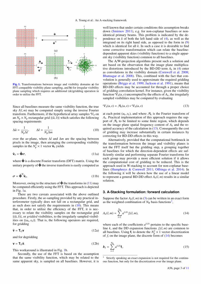
Fig. 1. Transformations between image and visibility domains a) forFFT compatible visibility plane sampling, and b) for irregular visibilityplane sampling which requires an additional (de)gridding operation inorder to utilize the FFT.

Since all baselines measure the same visibility function, the truesky I(l,m) may be computed simply using the inverse Fouriertransform. Furthermore, if the hypothetical array samplesV0 onan Np × Np rectangular grid (u, v) which satisfies the followingspacing requirements

∆u =1

Np∆l, ∆v =

1Np∆m

(10)

over the uv-plane, where ∆l and ∆m are the spacing betweenpixels in the image, then arranging the corresponding visibilitysamples in the N2

p × 1 vector v0 yields

v0 = Φσ, (11a)

where Φ is a discrete Fourier transform (DFT) matrix. Using theunitary property of Φ the inverse transform is easily computed as

σ = ΦH

v0. (11b)

Moreover, owing to the structure of Φ the transforms in (11) maybe computed efficiently using the FFT. This approach is depictedin Fig. 1a.

There are two caveats associated with the above outlinedprocedure. Firstly, the uv-sampling provided by any practical in-terferometer typically does not fall on a rectangular grid, andas such does not satisfy the requirements in (10). This meansthat, in order to utilize the efficiency of the FFT, it is nec-essary to relate the visibility samples on the rectangular grid(u, v), or gridded visibilities, to the irregularly sampled visibil-ities on (uk, vk). That is, the following operators are required,for gridding

v = TGv (12a)

and for degridding

v = TDv. (12b)

This workaround is illustrated in Fig. 1b.Secondly, the use of the FFT is based on the assumption

that the same visibility function, which may be related to thesame apparent sky, is sampled on all baselines. However, it is

well known that under certain conditions this assumption breaksdown (Smirnov 2011), e.g. for non-coplanar baselines or non-identical primary beams. This problem is indicated by the de-pendence on k of both the left hand side of (4), as well as theintegrand on its right hand side, as opposed to the form in (9)which is identical for all k. In such a case it is desirable to findsome corrective transformation which can relate the baseline-dependent apparent skies (visibility functions) to a single appar-ent sky (visibility function) common to all baselines.

The A/W-projection algorithms present such a solution andare based on the observation that the image plane multiplica-tive distortions introduced by the BD-DD term Ak in (4) enteras convolutions in the visibility domain (Cornwell et al. 2008;Bhatnagar et al. 2008). This, combined with the fact that con-volution is generally used to approximate the required griddingoperations (Briggs et al. 1999; Jackson et al. 1991), means thatBD-DD effects may be accounted for through a proper choiceof gridding convolution kernel. For instance, given the visibilityfunctionV0(u, v) uncorrupted by the effects of Ak, the irregularlysampled visibilities may be computed by evaluating

Vk(u, v) = Ak(u, v) ∗ V0(u, v) (13)

at each point (uk, vk), and where Ak is the Fourier transform ofAk. Practical implementation of this approach requires the sup-port of Ak to be limited to some finite region, which dependson the image plane spatial frequency content of Ak and the re-quired accuracy of the calculation in (13). Consequently the costof gridding may increase substantially in certain instances bycorrecting for BD-DD effects in this way.

Alternatively, provided that the computational bottleneck inthe transformation between the image and visibility planes isnot the FFT itself but the gridding step, a grouping togetherof baselines for which the direction-dependent effects are suf-ficiently similar and performing separate Fourier transforms foreach group may provide a more efficient solution if it allowsthe computational cost of gridding to be reduced. This is theapproach used in W-stacking to account for non-coplanar base-lines (Humphreys & Cornwell 2011; Offringa et al. 2014). Inthe following it will be shown how the use of a linear modelto represent a general BD-DD effect Ak(l,m) results in a similarsolution.

3. A-Stacking formulation: forward calculation

Suppose the factor Ak(l,m) in (3) can be written in an exact formas the weighted combination of NB basis functions3,

Ak(l,m) =

NB∑i=1

a(i,k) fi(l,m), (14)

where each of the coefficients a(i,k) pertains to the specific base-line k, and the DD expansion functions fi(l,m) are common toall baselines. Using fi to denote the N2

p × 1 vector discretizationof fi on the image plane, the discrete form of (14) becomes

bk =

NB∑i=1

a(i,k)fi. (15)

3 Strictly speaking an exact expansion is not required for the continu-ous function, but only for the discretization over the image plane.

A56, page 3 of 11

A&A 577, A56 (2015)

Substituting this expression into (5) gives

Vk(uk, vk) = φTk

NB∑

i=1

a(i,k)fi

σ =

NB∑i=1

a(i,k)φTk (fi σ)

=

NB∑i=1

a(i,k)φTk diag (fi)σ. (16)

Using ai =[a(i,1) a(i,2) · · · a(i,K)

]Tthe result for all baselines

can be written as

v =

NB∑i=1

ai [Φ (fi σ)

]=

NB∑i=1

diag (ai)Φ diag (fi)σ, (17)

which is the desired form relating the visibilities to the dis-cretized sky.

Equation (17) states that the visibilities pertaining to a modelsky may be calculated as follows, while fully accounting for theBD-DD effects contained in Ak:

1. Apply a per basis function image domain correction in theform of an element-wise multiplication to calculate a corre-sponding apparent sky,

σi = diag (fi)σ. (18a)

2. Fourier transform each apparent sky using the FFT, followedby a degridding step, to compute per basis function sets ofvisibilities,

vi = Φσi (18b)vi = TDvi. (18c)

3. Apply a visibility domain correction in the form of anelement-wise multiplication to each visibility set, and sumthe resulting visibility sets,

v =

NB∑i=1

diag (ai) vi. (18d)

Extension of the above results to include the full-polarizationresponse in the forward calculation is straightforward, and sim-ply uses a separate model similar to (14) for each of the sixteenelements in Ak.

3.1. Computational complexity

In order to identify conditions under which A-stacking maypresent an efficient alternative to a convolution based approachfor the forward calculation, the computational complexity of thealgorithm is compared here to that of A-projection. The algo-rithms are illustrated in Fig. 2.

Assuming a gridding convolution kernel of size Ng × Ng

is required to meet dynamic range requirements (Duijndam &Schonewille 1999), the overall cost incurred by (18) can beshown to scale as

O (CA-stack) = NB(N2p + N2

p log Np) + NBKN2g , (19)

where the first term on the right-hand side accounts for the perbasis function image plane correction and FFT, and second term

accounts for the gridding and visibility plane correction. In com-parison the overall cost of an A-projection implementation, as-suming a convolution kernel of size NgA×NgA is required to accu-rately account for the associated DD effects, scales as (Jongeriuset al. 2014; Offringa et al. 2014)

O(CA-proj

)= N2

p log Np + KN2gA. (20)

If the overall cost in both cases is dominated by the griddingstep, that is

KN2gA,KN2

g N2p log Np, (21)

then A-stacking presents a more efficient alternative toA-projection on condition that

NB <

(NgA

Ng

)2

· (22)

The total storage required to perform the A-stacking forward cal-culation in Fig. 2a completely in memory scales as

O (MA-stack) = NBN2p + N2

g + NBK, (23)

where the first term accounts for the per basis function imagedomain correction, the second accounts for the storage of thesingle gridding convolution kernel, and the last term accountsfor the per basis function visibility domain corrections. In com-parison, the total storage required to perform the A-projectionforward calculation in Fig. 2b completely in memory scales as

O(MA-proj

)= N2

p + KN2gA + K. (24)

Here storage of only a single image and visibility map arerequired, however a (potentially) different convolution ker-nel needs to be stored per baseline. The storage required orA-stacking is less than that for A-projection if

NB <KN2

gA + N2p − N2

g

N2p + K

≈

KN2

p + K

N2gA, (25)

where the approximation assumes that gridding dominates thecomputational cost as in (21) (which implies that KN2

gA N2p ),

and that N2g KN2

gA.Since NgA depends on the spatial frequency content of the

primary beam patterns on the sky, and NB depends on the inter-element variation among the primary beams, a clear distinctionbetween cases where one algorithm should outperform the other(in the asymptotic limit) in terms of computing time and mem-ory requirements is possible in principle. We also note that thecost of a convolution-based approach scales quadratically withan increase in NgA , whereas that of the stacking approach in (18)scales linearly with an increase in NB. This means that even witha moderately sized NgA a relatively large number of basis func-tions NB may still render the proposed method more efficient.

Finally, since the efficiency of A-stacking depends on reduc-ing the required size of the visibility plane convolution kernel,it may be necessary to avoid a convolution based approach tocorrect for non-coplanar baselines. As stated earlier, the w-termis easily included in the BD-DD modeling approach presentedhere, however, this may increase the number NB of terms in (14)required to yield an accurate model. Alternatively, A-stackingmay be combined with W-stacking (Offringa et al. 2014), whichdoes not affect the cost of gridding, but does result in the numberof image plane corrections and FFTs increasing by a factor Nw

(number of w-layers). This means that the cost of repeated FFTsmay become more expensive than gridding for fewer Nw thanwhen combing W-stacking with A-projection in the so-called hy-brid w-stacking (see Tasse et al. 2013).

A56, page 4 of 11

A. Young et al.: An A-stacking framework

σ

σ 1

σ 2

σ NB

...

×f1

×f2

×fNB

v1

v2

vNB

...

Φ

Φ

Φ

∗∗

∗

Ng ×Ng

...

=

=

=

v1

v2

vNB

...

×a1

×a2

×aNB

=v

fghijklmnopqrst

Step 1

abcdefabcdefghijklmnopqrstuvwxyzstuvwxyz

Step 2

defghijklmnopqrstuvwx

Step 3

(a) A-stacking

σ vΦ

∗∗

∗

ghij

klm

nop

qrst

...

NgA ×NgA

=

=

=

...

ghij

klm

nop

qrst

=

v

(b) A-projection

Fig. 2. a) Forward calculation in the A-stacking framework, subdivided into the algorithmic steps described by (18). b) Forward calculation usingA-projection. The A-projection convolution kernel size is NgA × NgA , as determined by the spatial frequency content of the direction-dependenteffects on the sky, and can result in a relatively expensive gridding cost. A-stacking aims to reduce this cost by decreasing the size of the griddingconvolution kernel to Ng × Ng, as determined by the required image dynamic range; the penalty is that multiple FFTs and gridding operations arerequired.

4. Imaging with A-stacking: backward calculation

Imaging is concerned with the inversion of (7). As was alreadystated, the scale of this system of equations precludes the useof a direct method, so that a different approach to imaging isrequired. In this section two approaches possible within theA-stacking framework are derived.

4.1. Adaptation to the CLEAN algorithm

In theory, the Fourier relationship in (4) allows the apparentsky Ik to be determined from the visibility functionVk via the in-verse Fourier transform. Given the discretization inherent to thelimited sampling provided by any practical interferometer arrayand the image representation of the sky, the result of the practicalequivalent of this is

σd =1KΦHv =

1KΦH (Φ B

)σ, (26)

which is the so-called dirty image4. Apart from the effects as-sociated with B, the limited sampling of the array also adds adistortion in the form of a convolution with the Fourier trans-form of the visibility plane sampling function, or point spreadfunction (PSF) (Jackson et al. 1991). Not only does this limitthe resolution of the obtained image to the scale of the PSF mainlobe, but sidelobes in the PSF can also produce artifacts that mayproduce false sources, hide existing ones, or distort other sourcesin the image. Removing this corruption requires some deconvo-lution procedure. However, owing to the imperfect sampling of

4 In practice this is usually calculated via gridding and applying theFFT, i.e. σd = 1

K Φv. For the purposes of the present derivation calcula-tion of the dirty image via the direct Fourier transform is used.

the array in general the solution is not unique, so that a non-linear deconvolution procedure is usually required (Cornwellet al. 1999). The algorithm perhaps most widely used for thispurpose is CLEAN and its derivatives (Högbom 1974; Clark1980; Schwab 1984). In general this algorithm is based on iden-tifying a peak in the dirty image as the location of a point-likesource, and then removing the effect of that source by subtract-ing an appropriately scaled and shifted PSF.

In order to demonstrate how this algorithm may be adaptedwithin the A-stacking framework, we consider the dirty imageproduced by applying ΦH to the visibilities in (17)

σd =1KΦHv =

1KΦH

NB∑i=1

diag (ai)Φ diag (fi)σ

=1K

NB∑i=1

ΦH diag (ai)Φ diag (fi)σ. (27)

Replacing the true sky image vector σ with an image es corre-sponding to a single point source of unit intensity at the location(ls,ms) and an otherwise empty sky, yields the PSF

ps =

NB∑i=1

fi(ls,ms)[

1KΦH diag (ai)Φes

]

=

NB∑i=1

fi(ls,ms)qi(s). (28)

Herein qi(s) is the PSF, centered at (ls,ms), and associated withapplying the weights ai to the visibilities. Although each qi rep-resents a shift-invariant PSF, that represented by ps is not shift-invariant, because of the direction-dependent weighting fi(ls,ms)

A56, page 5 of 11

A&A 577, A56 (2015)

applied to each qi. Assuming a sky composed of a number Ns ofpoint sources allows the following representation

σ =

Ns∑s=1

σ(s)es (29)

which, when substituted into (27) and using (28) gives the de-sired result,

σd =

NB∑i=1

Ns∑s=1

σ(s) fi(ls,ms)qi(s) =

Ns∑s=1

σ(s)ps. (30)

This expression presents an interesting decomposition of thedirty image: it is the superposition of a number of sub-images,each of which is a different apparent sky σi convolved with anassociated PSF qi. More importantly, this interpretation can beused to adapt the PSF subtraction in the CLEAN algorithm toaccount more accurately for the BD-DD effects.

We let the NB different PSFsqi

NBi=1 be pre-computed as part

of initializing the CLEAN algorithm, and we let σr be the resid-ual dirty image at the start of a PSF subtraction iteration. Witha point source identified at location s in σr the PSF subtractionnow proceeds as follows:

1. Weigh each PSF qi(s) by the value of its corresponding DDbasis function towards the direction of the source fi(ls,ms),and accumulate the result for all NB basis functions to yieldthe total PSF ps as in (28).

2. Scale ps according to the intensity of the identified sourceand the loop gain parameter γ,

ps ← γσ(s)r ps. (31a)

3. Update the residual image by subtracting the PSF,

σr ← σr − ps. (31b)

Combining the above procedure with the forward calculationin (18) provides an accurate method by which BD-DD effectsmay be accounted for in the imaging process.

4.2. Diagonal correction

Using the BD-DD effect model in (14) also produces a usefulimaging approach for the case where deconvolution is not neces-sary, either because the image dynamic range is not high enoughor because the spatial selectivity is very good, so that artifactsproduced by the PSF sidelobe structure do not have a dominanteffect on the image quality.

Suppose an overdetermined system in (7), that is, K > N2p .

The well-known linear least squares (LLS) solution to such asystem is

σ =(Φ B

)† v =[(Φ B

)H (Φ B

)]−1 (Φ B

)H v, (32)

where † denotes the Moore-Penrose pseudoinverse. Using themodel in (15) and the result in (17), the LSS solution becomes

σ = M−1σd, (33)

where the deconvolution matrix M−1 and the dirty image vector5

σd have been introduced,

M =

NB∑j=1

diag(a j

)Φ diag

(f j

)H NB∑

i=1

diag (ai)Φ diag (fi)

=

NB∑i=1

NB∑j=1

diag(f j)HΦH diag(a j)H diag (ai)Φ diag (fi) (34a)

σd =

NB∑i=1

diag (ai)Φ diag (fi)

H

v. (34b)

Because of the computational costs involved for typically en-countered image sizes, direct evaluation of (33) may not be prac-ticable. However, given the condition that deconvolution is un-necessary, the inversion of M becomes tractable in that it may beapproximated as being diagonal6. This results from the fact thatthe off-diagonal entries in this matrix represent the flux leakagebetween different pixels in the image, the very effect deconvolu-tion aims to correct.

We let Mdiag be the matrix formed by setting all off-diagonalentries in M equal to zero. In order to determine the structure ofthis matrix, we consider the qth diagonal element in[ΦH diag(a j)H diag (ai)Φ

](q,q)=

K∑k=1

Φ(k,q)a( j,k)a(i,k)Φ(k,q)

= aHj ai, (35)

where the relation Φ(k,q)Φ(k,q) = 1 has been used. Since the resultis independent of q, we can write

Mdiag =

NB∑i=1

NB∑j=1

diag(f j)H[aH

j aiI]

diag (fi)

=

NB∑i=1

NB∑j=1

aHj ai diag

(f j fi

), (36)

since aHj ai is scalar, and where I is an appropriately sized iden-

tity matrix.This naturally leads to the following imaging procedure:

1. Compute the dirty image σd,i for each basis function by ap-plying the weights ai to the visibilities, Fourier transformingto the image plane (via gridding and using the FFT), and thenweighting the image values by fi,

σd,i = diag(fi)H[Φ

HTG

(diag(ai)Hv

)]. (37a)

This is simply a practical implementation of each termin (34b).

2. Accumulate the result for the NB basis functions to yield thedirty image,

σd =

NB∑i=1

σd,i. (37b)

5 This is not the same dirty image as in (26).6 In fact, the diagonal approximation may also be used to speed updeconvolution via an optimization procedure such as the Levenberg-Marquardt algorithm (Marquardt 1963). Such an approximation reducesthe Jacobian (and hence the approximate Hessian) of the deconvolutionproblem σ = M−1σd to a diagonal matrix, which reduces the order ofcomplexity of the algorithm from O(N6

p ) to O(N4p ).

A56, page 6 of 11

A. Young et al.: An A-stacking framework

3. Compute the diagonal version of the deconvolution matrixMdiag using (36).

4. Compute the final result,

σdiag = M−1diagσd. (37c)

5. Basis function construction

Although the above results are generally applicable for any exactexpansion of Ak which has the form of (14), it is obviously desir-able to obtain such an expansion which requires the least numberof terms, since the cost of the above derived algorithms generallyscale with NB. In this section an approach aimed at producingsuch a model from a prior characterized Ak is presented.

For imaging purposes it is sufficient to obtain a model forthe discretization of Ak on the image grid, that is bk as in (15).From (8a) it is clear that finding a set of expansion func-tions fi

NBi=1 with which each bk may be expressed as in (15) is

equivalent to finding a basis for the row space of B. One such ba-sis may be obtained by computing the truncated Singular ValueDecomposition (SVD),

BT = UΣWH. (38)

Selecting the columns in the N2p×NB matrix U (left-singular vec-

tors) as the basis functions fi in (15), it can be shown that eachexpansion coefficient a(i,k) is the entry on the ith row and kthcolumn in the matrix7

a = UHBT = ΣWH. (39)

This produces an exact expansion with NB ≤ min(N2

p ,K)

num-ber of terms, where the inequality may result from a lineardependence among the DD gains associated with each of thebaselines8.

Since the computational burden resulting from the use ofthe linear model in (15) scales linearly with the number ofbasis functions, it may be desirable to rather use nB < NBnumber of terms, thus trading computational cost for accuracy.Furthermore, since the accuracy of transformations between theimage and visibility planes is also affected by other factors (e.g.noise, gridding/degridding), the required accuracy may need tobe only such that it does not limit the overall accuracy. Withthese considerations in mind, the aim is to produce a modelwhich yields the highest precision for a given number of terms.For this reason, the model provided through the use of the SVDis especially useful in the case where nB < NB. Specifically,the sum of the squared distances between each of the rows in Band the vector space spanned by nB left-singular vectors is min-imized by choosing those left-singular vectors corresponding tothe nB largest singular values on the diagonal of Σ (Jolliffe 1986).

It should be noted that the computational cost incurred byevaluating (38) and (39) does not need to enter into the over-all cost of the algorithms presented in the previous sections,since the result need only be determined once and can be stored

7 The rows in a are mutually orthogonal owing to the unitary propertyof W, so that aH

j ai = 0 for i , j. This result may be used to reduce thecomplexity of evaluating (36) from O(N2

B) to O(NB).8 For instance, this may apply to earth rotation synthesis where mul-tiple visibility measurements are obtained between the same antennapair, resulting in identical rows in B. Even when the primary beams arevarying in time, e.g. rotating primary beams on the sky for alt-az mountreflector antennas, a linear dependence will still be present if such varia-tion is negligible over time scales much larger than the integration time.

for repeated use over the course of one or more observations9.Nevertheless, one way to alleviate the cost of constructing theBD-DD model is to sample Ak over a sparser grid prior to com-puting the basis functions. The motivation for this approach isthat the resolution obtainable with the entire array may be muchhigher than that required to accurately represent the radiationpattern of a single antenna element in such an array. We let b′k besuch a discretization of Ak over an Nq × Nq grid (l′,m′) in theimage plane, where Np = αNq with α > 1, and

Np∆l = Nq∆l′, Np∆m = Nq∆m′. (40)

Using this discretization of the BD-DD effects the matrix B′

is constructed, and the SVD is computed to yield NB ≤

min(N2

q ,K)

left-singular vectors f′iNBi=1. The model basis func-

tions are now obtained by first interpolating each singular vectorto extend its support onto the Np × Np grid,

TI : (l′,m′) → (l,m) , gi = TI(f′i), (41)

and then orthonormalizing the resulting set of vectors to yieldfi

NBi=1. Each model coefficient a(i,k) is then computed by project-

ing the ith basis function onto the kth column of BT.

6. Results

In this section simulation results are presented in order to as-sess the performance of the A-stacking approach. First the im-pact of various factors on the accuracy of the forward calculationis considered, followed by a demonstration of the performanceof the CLEAN algorithm when combined with the A-stackingapproach.

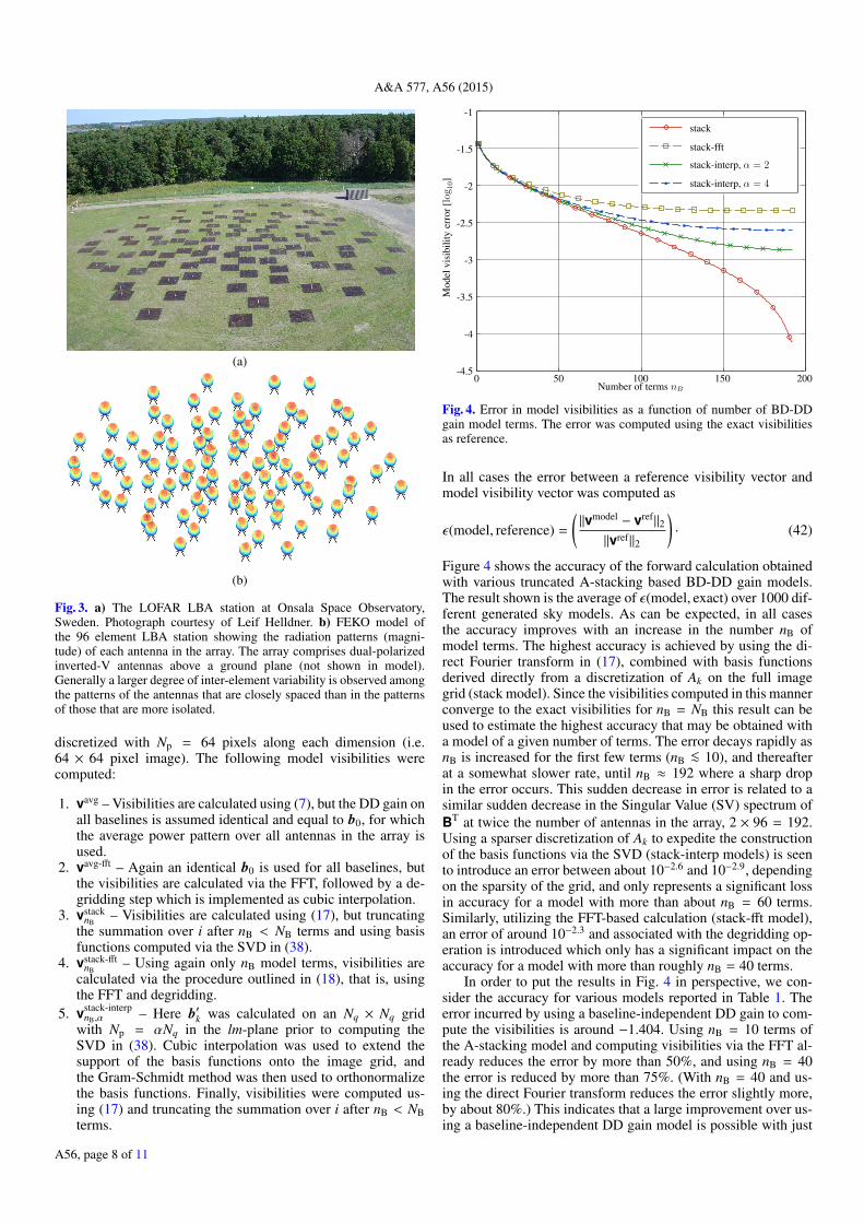
Simulations pertain to a snapshot observation in a narrowfrequency band around 50 MHz, using one polarization of theLOFAR Low Band Antenna (LBA) station at Onsala, Sweden asan interferometer array. A full-wave numerical model was ana-lyzed in FEKO10 to determine the radiation patterns of all theelements in the array (Young et al. 2014); see Fig. 3. Becauseof the effects of mutual coupling, which was fully accountedfor in the numerical model, the primary beams exhibited a vari-ation over the elements in the array so that a single primarybeam approximation would not suffice. The phase reference foreach pattern was located at the corresponding antenna position inthe array, as used to determine the baseline uv-coordinates. Skymodels were generated by randomly placing ten point sourcesof varying intensity on an image grid, so that the source statis-tics were in agreement with that reported in Bregman (2012)for frequencies below 1.4 GHz. The sky models were then usedas input to various observation simulations. For each simula-tion the reference (exact) visibilities vexact were calculated viadirect evaluation of (7), which were then used as input for fur-ther analysis.

6.1. Accuracy of the forward calculation

Model visibilities were calculated from the input sky using var-ious approaches, and then compared to the exact visibilities.The sky model extended over the region |l|, |m| ≤ 0.5 and was

9 The caveat here is that, where the BD-DD effects are unknown andalso need solution, the solvable model may need to be in an appropriateform to allow precomputing (38) and (39). This is not within the scopeof the present contribution and is the focus of ongoing work.10 https://www.feko.info/

A56, page 7 of 11

A&A 577, A56 (2015)

(a)

(b)

Fig. 3. a) The LOFAR LBA station at Onsala Space Observatory,Sweden. Photograph courtesy of Leif Helldner. b) FEKO model ofthe 96 element LBA station showing the radiation patterns (magni-tude) of each antenna in the array. The array comprises dual-polarizedinverted-V antennas above a ground plane (not shown in model).Generally a larger degree of inter-element variability is observed amongthe patterns of the antennas that are closely spaced than in the patternsof those that are more isolated.

discretized with Np = 64 pixels along each dimension (i.e.64 × 64 pixel image). The following model visibilities werecomputed:

1. vavg – Visibilities are calculated using (7), but the DD gain onall baselines is assumed identical and equal to b0, for whichthe average power pattern over all antennas in the array isused.

2. vavg-fft – Again an identical b0 is used for all baselines, butthe visibilities are calculated via the FFT, followed by a de-gridding step which is implemented as cubic interpolation.

3. vstacknB

– Visibilities are calculated using (17), but truncatingthe summation over i after nB < NB terms and using basisfunctions computed via the SVD in (38).

4. vstack-fftnB

– Using again only nB model terms, visibilities arecalculated via the procedure outlined in (18), that is, usingthe FFT and degridding.

5. vstack-interpnB,α – Here b′k was calculated on an Nq × Nq grid

with Np = αNq in the lm-plane prior to computing theSVD in (38). Cubic interpolation was used to extend thesupport of the basis functions onto the image grid, andthe Gram-Schmidt method was then used to orthonormalizethe basis functions. Finally, visibilities were computed us-ing (17) and truncating the summation over i after nB < NBterms.

0 50 100 150 200-4.5

-4

-3.5

-3

-2.5

-2

-1.5

-1

Number of terms nB

Modelvisibilityerror[log10]

stack

stack-fft

stack-interp, α = 2

stack-interp, α = 4

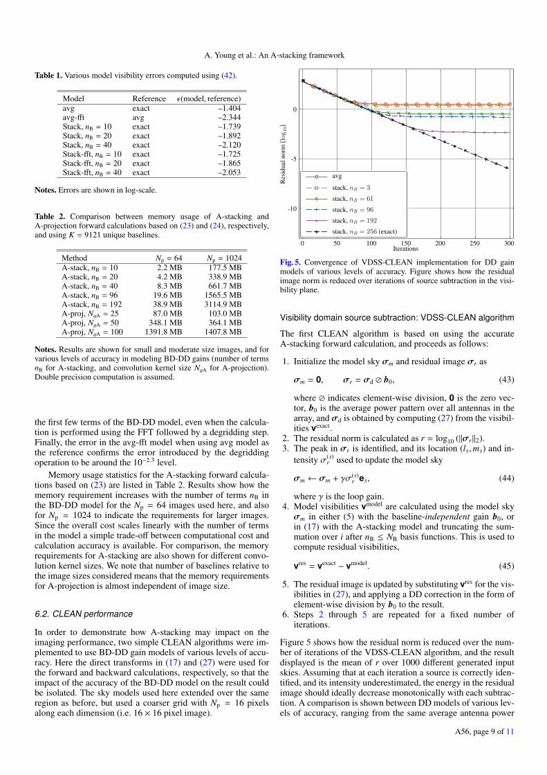
Fig. 4. Error in model visibilities as a function of number of BD-DDgain model terms. The error was computed using the exact visibilitiesas reference.

In all cases the error between a reference visibility vector andmodel visibility vector was computed as

ε(model, reference) =

(‖vmodel − vref‖2

‖vref‖2

)· (42)

Figure 4 shows the accuracy of the forward calculation obtainedwith various truncated A-stacking based BD-DD gain models.The result shown is the average of ε(model, exact) over 1000 dif-ferent generated sky models. As can be expected, in all casesthe accuracy improves with an increase in the number nB ofmodel terms. The highest accuracy is achieved by using the di-rect Fourier transform in (17), combined with basis functionsderived directly from a discretization of Ak on the full imagegrid (stack model). Since the visibilities computed in this mannerconverge to the exact visibilities for nB = NB this result can beused to estimate the highest accuracy that may be obtained witha model of a given number of terms. The error decays rapidly asnB is increased for the first few terms (nB <∼ 10), and thereafterat a somewhat slower rate, until nB ≈ 192 where a sharp dropin the error occurs. This sudden decrease in error is related to asimilar sudden decrease in the Singular Value (SV) spectrum ofBT at twice the number of antennas in the array, 2 × 96 = 192.Using a sparser discretization of Ak to expedite the constructionof the basis functions via the SVD (stack-interp models) is seento introduce an error between about 10−2.6 and 10−2.9, dependingon the sparsity of the grid, and only represents a significant lossin accuracy for a model with more than about nB = 60 terms.Similarly, utilizing the FFT-based calculation (stack-fft model),an error of around 10−2.3 and associated with the degridding op-eration is introduced which only has a significant impact on theaccuracy for a model with more than roughly nB = 40 terms.

In order to put the results in Fig. 4 in perspective, we con-sider the accuracy for various models reported in Table 1. Theerror incurred by using a baseline-independent DD gain to com-pute the visibilities is around −1.404. Using nB = 10 terms ofthe A-stacking model and computing visibilities via the FFT al-ready reduces the error by more than 50%, and using nB = 40the error is reduced by more than 75%. (With nB = 40 and us-ing the direct Fourier transform reduces the error slightly more,by about 80%.) This indicates that a large improvement over us-ing a baseline-independent DD gain model is possible with just

A56, page 8 of 11

A. Young et al.: An A-stacking framework

Table 1. Various model visibility errors computed using (42).

Model Reference ε(model, reference)avg exact –1.404avg-fft avg –2.344Stack, nB = 10 exact –1.739Stack, nB = 20 exact –1.892Stack, nB = 40 exact –2.120Stack-fft, nB = 10 exact –1.725Stack-fft, nB = 20 exact –1.865Stack-fft, nB = 40 exact –2.053

Notes. Errors are shown in log-scale.

Table 2. Comparison between memory usage of A-stacking andA-projection forward calculations based on (23) and (24), respectively,and using K = 9121 unique baselines.

Method Np = 64 Np = 1024A-stack, nB = 10 2.2 MB 177.5 MBA-stack, nB = 20 4.2 MB 338.9 MBA-stack, nB = 40 8.3 MB 661.7 MBA-stack, nB = 96 19.6 MB 1565.5 MBA-stack, nB = 192 38.9 MB 3114.9 MBA-proj, NgA = 25 87.0 MB 103.0 MBA-proj, NgA = 50 348.1 MB 364.1 MBA-proj, NgA = 100 1391.8 MB 1407.8 MB

Notes. Results are shown for small and moderate size images, and forvarious levels of accuracy in modeling BD-DD gains (number of termsnB for A-stacking, and convolution kernel size NgA for A-projection).Double precision computation is assumed.

the first few terms of the BD-DD model, even when the calcula-tion is performed using the FFT followed by a degridding step.Finally, the error in the avg-fft model when using avg model asthe reference confirms the error introduced by the degriddingoperation to be around the 10−2.3 level.

Memory usage statistics for the A-stacking forward calcula-tions based on (23) are listed in Table 2. Results show how thememory requirement increases with the number of terms nB inthe BD-DD model for the Np = 64 images used here, and alsofor Np = 1024 to indicate the requirements for larger images.Since the overall cost scales linearly with the number of termsin the model a simple trade-off between computational cost andcalculation accuracy is available. For comparison, the memoryrequirements for A-stacking are also shown for different convo-lution kernel sizes. We note that number of baselines relative tothe image sizes considered means that the memory requirementsfor A-projection is almost independent of image size.

6.2. CLEAN performance

In order to demonstrate how A-stacking may impact on theimaging performance, two simple CLEAN algorithms were im-plemented to use BD-DD gain models of various levels of accu-racy. Here the direct transforms in (17) and (27) were used forthe forward and backward calculations, respectively, so that theimpact of the accuracy of the BD-DD model on the result couldbe isolated. The sky models used here extended over the sameregion as before, but used a coarser grid with Np = 16 pixelsalong each dimension (i.e. 16 × 16 pixel image).

0 50 100 150 200 250 300

-10

-5

0

Iterations

Residualnorm

[log10]

avg

stack, nB = 3

stack, nB = 61

stack, nB = 96

stack, nB = 192

stack, nB = 256 (exact)

Fig. 5. Convergence of VDSS-CLEAN implementation for DD gainmodels of various levels of accuracy. Figure shows how the residualimage norm is reduced over iterations of source subtraction in the visi-bility plane.

Visibility domain source subtraction: VDSS-CLEAN algorithm

The first CLEAN algorithm is based on using the accurateA-stacking forward calculation, and proceeds as follows:

1. Initialize the model sky σm and residual image σr as

σm = 0, σr = σd b0, (43)

where indicates element-wise division, 0 is the zero vec-tor, b0 is the average power pattern over all antennas in thearray, and σd is obtained by computing (27) from the visibil-ities vexact.

2. The residual norm is calculated as r = log10 (‖σr‖2).3. The peak in σr is identified, and its location (ls,ms) and in-

tensity σ(s)r used to update the model sky

σm ← σm + γσ(s)r es, (44)

where γ is the loop gain.4. Model visibilities vmodel are calculated using the model skyσm in either (5) with the baseline-independent gain b0, orin (17) with the A-stacking model and truncating the sum-mation over i after nB ≤ NB basis functions. This is used tocompute residual visibilities,

vres = vexact − vmodel. (45)

5. The residual image is updated by substituting vres for the vis-ibilities in (27), and applying a DD correction in the form ofelement-wise division by b0 to the result.

6. Steps 2 through 5 are repeated for a fixed number ofiterations.

Figure 5 shows how the residual norm is reduced over the num-ber of iterations of the VDSS-CLEAN algorithm, and the resultdisplayed is the mean of r over 1000 different generated inputskies. Assuming that at each iteration a source is correctly iden-tified, and its intensity underestimated, the energy in the residualimage should ideally decrease monotonically with each subtrac-tion. A comparison is shown between DD models of various lev-els of accuracy, ranging from the same average antenna power

A56, page 9 of 11

A&A 577, A56 (2015)

Table 3. Mean residual norms (log-scale) after 300 iterations of eachCLEAN algorithm for various BD-DD models.

Model VDSS-CLEAN IDSS-CLEANavg 0.445 0.721stack, nB = 3 0.298 0.569stack, nB = 61 –0.516 –0.129stack, nB = 96 –0.825 –0.422stack, nB = 192 –2.387 –1.915stack, nB = 256 –6.076 –4.610

Table 4. Image dynamic range after 300 iterations of each CLEAN al-gorithm for various BD-DD models.

Model VDSS-CLEAN IDSS-CLEANavg 32.8 dB 24.0 dBstack, nB = 3 34.3 dB 25.5 dBstack, nB = 61 42.4 dB 32.5 dBstack, nB = 96 45.5 dB 35.5 dBstack, nB = 192 61.1 dB 50.4 dBstack, nB = 256 98.0 dB 77.3 dB

pattern over all baselines (avg) to the exact A-stacking model(stack, nB = NB = 256). The intermediate models correspondto keeping only those terms corresponding to Singular Values(SVs) in (38) that are above 1.0% (nB = 3) and 0.1% (nB = 61)relative to the maximum; nB = 96 uses as many terms in themodel as antennas in the array, and nB = 192 uses twice as manyterms. The latter model is of interest since the SV spectrum ex-hibits a sharp drop after the 192th SV. In general the algorithmis seen to converge at ever lower values of the residual normas the model accuracy is increased. The results for each modelafter the final iteration are summarized in Table 3. Comparedto the result for using the average DD gain, using A-stackingwith just 3 terms the residual is reduced by about 29%, and with61 terms by 89%.

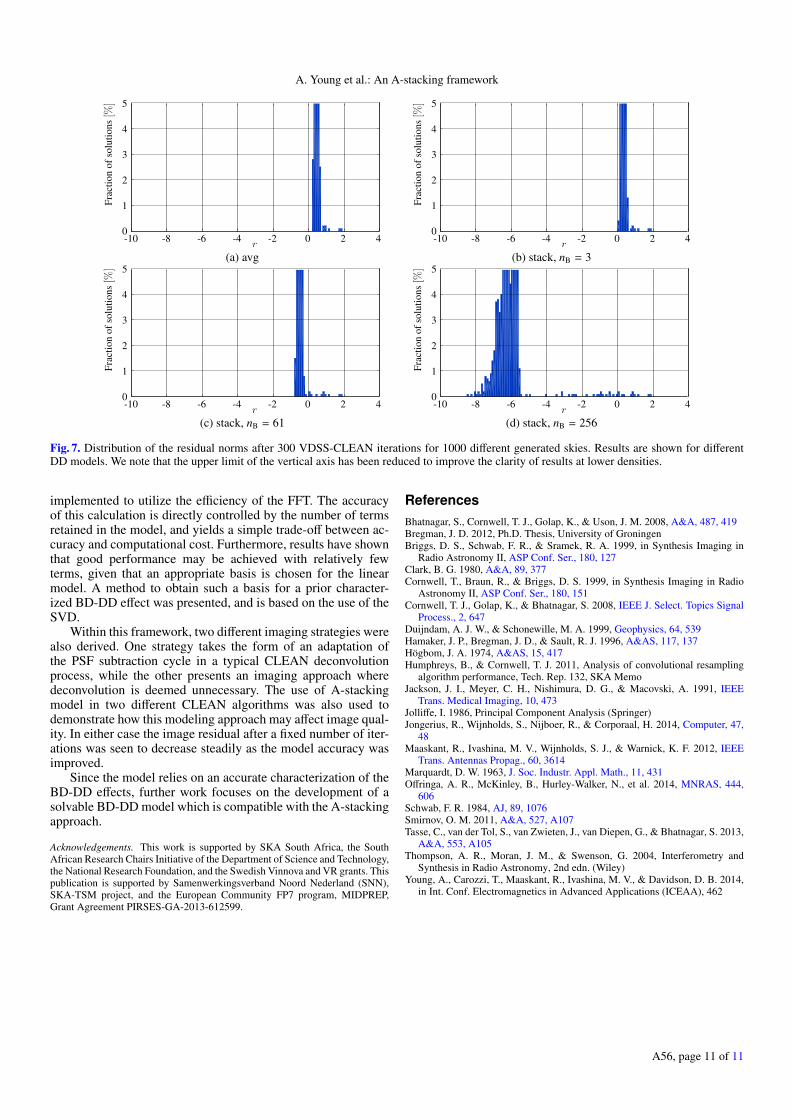
The distributions of residual norms after 300 iterations andfor all 1000 simulations are shown in Fig. 7 for four differentDD models. In 95% of the simulations the average beam modelyielded r < 0.55, and the A-stack model with nB = 3 andnB = 61 yielded r < 0.45, and r < −0.35, respectively. Usingthe exact model resulted in r < −5.65 for the same percentageof simulations. For a small fraction of the simulations the algo-rithm converged to a relatively large residual irrespective of theDD gain model used.

Image domain source subtraction: IDSS-CLEAN algorithm

The second CLEAN implementation is based on the proce-dure outlined in (31) from Sect. 4.1. Using the measured vis-ibilities vexact the dirty image is computed using (27), and theresidual image σr is initialized to this dirty image without anyDD correction as was done for the VDSS-CLEAN algorithm.The algorithm then proceeds by repeatedly performing PSFsubtraction via (31) to update σr for a fixed number of itera-tions, and computing the residual norm r = log10(‖σr‖) at eachiteration.

Figure 6 shows how the residual norm is reduced over thenumber of iterations for the IDSS-CLEAN algorithm. The resultshown is the mean of r over 1000 different generated sky modelsand a comparison is shown for various DD gain models. Initiallythe residual decreases at a steady rate for all DD gain mod-els; beyond a certain number of iterations this decrease slowsdown significantly, and the residual level at which this occurs

0 200 400 600

-10

-5

0

Iterations

Residualnorm

[log10]

avg

stack, nB = 3

stack, nB = 61

stack, nB = 96

stack, nB = 192

stack, nB = 256 (exact)

Fig. 6. Convergence of IDSS-CLEAN implementation for DD gainmodels of various levels of accuracy. Figure shows how the residualimage norm is reduced over iterations of source subtraction in the im-age plane.

depends once again on the accuracy of the DD gain model. Forcomparison, the results after 300 iterations of IDSS-CLEAN forthe different gain models are also shown in Table 3. Apart fromsomewhat higher residuals after the same number of iterationsas compared to that in VDSS-CLEAN, the decrease in the resid-ual with the increase in the number of terms in the gain modelis similar for both algorithms. To help put these results into per-spective, the dynamic range of the images obtained after 300 it-erations of either CLEAN algorithm was calculated and listed inTable 4.

Assuming that a distinct source (in a distinct location) isidentified in each iteration of the IDSS-CLEAN algorithm, adifferently weighted combination of the PSFs associated witheach of the DD basis functions may be required at each itera-tion. This combination step requires up to NBN2

p complex mul-tiplications and is the computational bottleneck for this imagedomain deconvolution approach. As can be expected the cost ofa single iteration of this algorithm is much cheaper than that forthe VDSS-CLEAN algorithm, which includes an image domaincorrection that also scales as NBN2

p , as well as the costs associ-ated with transforming between the image and visibility planes.This holds even when utilizing the efficiency of an FFT-basedimplementation, see (19).

7. Conclusion

A novel framework for modeling baseline-dependent direction-dependent effects was presented. The approach is based onthe expansion of BD-DD effects in the form of a weightedsum of basis functions, where the basis functions are direction-dependent, and the coefficients account for the baseline-dependence. Related to the W-stacking method which ac-counts for non-coplanar baselines, the present approach, calledA-stacking, offers an alternative method to the convolutionbased algorithm A-projection. As such it offers a potentialimprovement in computational efficiency in scenarios whereA-projection results in a significant increase in the gridding cost.

Using the proposed modeling technique the calculationfrom sky to visibilities is achieved by combining the resultfrom a number of separate Fourier transforms, which may be

A56, page 10 of 11

A. Young et al.: An A-stacking framework

-10 -8 -6 -4 -2 0 2 40

1

2

3

4

5

r

Fractionofsolutions[%

]

-10 -8 -6 -4 -2 0 2 40

1

2

3

4

5

r

Fractionofsolutions[%

]

(a) avg (b) stack, nB = 3

-10 -8 -6 -4 -2 0 2 40

1

2

3

4

5

r

Fractionofsolutions[%

]

-10 -8 -6 -4 -2 0 2 40

1

2

3

4

5

r

Fractionofsolutions[%

](c) stack, nB = 61 (d) stack, nB = 256

Fig. 7. Distribution of the residual norms after 300 VDSS-CLEAN iterations for 1000 different generated skies. Results are shown for differentDD models. We note that the upper limit of the vertical axis has been reduced to improve the clarity of results at lower densities.

implemented to utilize the efficiency of the FFT. The accuracyof this calculation is directly controlled by the number of termsretained in the model, and yields a simple trade-off between ac-curacy and computational cost. Furthermore, results have shownthat good performance may be achieved with relatively fewterms, given that an appropriate basis is chosen for the linearmodel. A method to obtain such a basis for a prior character-ized BD-DD effect was presented, and is based on the use of theSVD.

Within this framework, two different imaging strategies werealso derived. One strategy takes the form of an adaptation ofthe PSF subtraction cycle in a typical CLEAN deconvolutionprocess, while the other presents an imaging approach wheredeconvolution is deemed unnecessary. The use of A-stackingmodel in two different CLEAN algorithms was also used todemonstrate how this modeling approach may affect image qual-ity. In either case the image residual after a fixed number of iter-ations was seen to decrease steadily as the model accuracy wasimproved.

Since the model relies on an accurate characterization of theBD-DD effects, further work focuses on the development of asolvable BD-DD model which is compatible with the A-stackingapproach.

Acknowledgements. This work is supported by SKA South Africa, the SouthAfrican Research Chairs Initiative of the Department of Science and Technology,the National Research Foundation, and the Swedish Vinnova and VR grants. Thispublication is supported by Samenwerkingsverband Noord Nederland (SNN),SKA-TSM project, and the European Community FP7 program, MIDPREP,Grant Agreement PIRSES-GA-2013-612599.

ReferencesBhatnagar, S., Cornwell, T. J., Golap, K., & Uson, J. M. 2008, A&A, 487, 419Bregman, J. D. 2012, Ph.D. Thesis, University of GroningenBriggs, D. S., Schwab, F. R., & Sramek, R. A. 1999, in Synthesis Imaging in

Radio Astronomy II, ASP Conf. Ser., 180, 127Clark, B. G. 1980, A&A, 89, 377Cornwell, T., Braun, R., & Briggs, D. S. 1999, in Synthesis Imaging in Radio

Astronomy II, ASP Conf. Ser., 180, 151Cornwell, T. J., Golap, K., & Bhatnagar, S. 2008, IEEE J. Select. Topics Signal

Process., 2, 647Duijndam, A. J. W., & Schonewille, M. A. 1999, Geophysics, 64, 539Hamaker, J. P., Bregman, J. D., & Sault, R. J. 1996, A&AS, 117, 137Högbom, J. A. 1974, A&AS, 15, 417Humphreys, B., & Cornwell, T. J. 2011, Analysis of convolutional resampling

algorithm performance, Tech. Rep. 132, SKA MemoJackson, J. I., Meyer, C. H., Nishimura, D. G., & Macovski, A. 1991, IEEE

Trans. Medical Imaging, 10, 473Jolliffe, I. 1986, Principal Component Analysis (Springer)Jongerius, R., Wijnholds, S., Nijboer, R., & Corporaal, H. 2014, Computer, 47,

48Maaskant, R., Ivashina, M. V., Wijnholds, S. J., & Warnick, K. F. 2012, IEEE

Trans. Antennas Propag., 60, 3614Marquardt, D. W. 1963, J. Soc. Industr. Appl. Math., 11, 431Offringa, A. R., McKinley, B., Hurley-Walker, N., et al. 2014, MNRAS, 444,

606Schwab, F. R. 1984, AJ, 89, 1076Smirnov, O. M. 2011, A&A, 527, A107Tasse, C., van der Tol, S., van Zwieten, J., van Diepen, G., & Bhatnagar, S. 2013,

A&A, 553, A105Thompson, A. R., Moran, J. M., & Swenson, G. 2004, Interferometry and

Synthesis in Radio Astronomy, 2nd edn. (Wiley)Young, A., Carozzi, T., Maaskant, R., Ivashina, M. V., & Davidson, D. B. 2014,

in Int. Conf. Electromagnetics in Advanced Applications (ICEAA), 462

A56, page 11 of 11