PCSWMM Evaluation - wrrc.umass.edu Depression Storage ... transpiration, or the evaporation of water from the vascular system of plants into the ... interception loses - typically

PCSWMM Evaluation Project # 08-08/319

Final Technical Report

Prepared by Dr. Paula Rees Jerry Schoen

Submitted by The Water Resources Research Center University of Massachusetts, Amherst MA 01003

July 31, 2009 Produced under contract with the Massachusetts Department of Environmental Protection.

II

This project has been financed with Federal Funds from the Environmental Protection Agency (EPA) to the Massachusetts Department of Environmental Protection (the Department) under an s. 319 competitive grant. The contents do not necessarily reflect the views and policies of EPA or of the Department, nor does the mention of trade names or commercial products constitute endorsement or recommendation for use. Acknowledgements The authors wish to express their thanks to Thomas Maguire of the Massachusetts Department of Environmental Protection for his consultation during the project and his review of document drafts.

III

Abstract The Massachusetts Department of Environmental Protection requires stormwater best management practices (BMPs) to be sized using a Water Quality Volume (WQV), either the first ½- or 1-inch of runoff. However, in engineering practice, some BMPs are best sized using a flow rate, and not WQV. Four methods were reviewed to convert the regulatory WQV used for sizing BMPs to a flow rate. The methods reviewed were a PC version of EPA’s Stormwater Management model, Ahlfeld et al 2004, Bryant undated, and Claytor et al 1996. It was found that the specific field studies used to corroborate the PCSWMM method do not contradict the results; however it was also found that those field studies were not robust enough to confirm the results with reasonable certainty. It was also found that none of the methods accounted for routing, flow path, and the effect of precipitation falling as snow, all of which play a role in transforming a runoff volume to a flow rate. Of the four methods reviewed, the Claytor at al 1996 method is the most complete in attempting to explicitly define the Water Quality Volume based on precipitation and site characterization as well as to transform the resulting depth to a flow rate. However, the first step of the Claytor method has not been completed specifically for Massachusetts. The Bryant and Claytor methods utilize the full record of available precipitation data in order to define an event-based design criteria upon which sizing is then based. The Ahlfeld method evaluates only periods of precipitation which meet the pre-defined WQV. In contrast to these methods, PCSWMM estimates runoff, sediment wash-off, and sediment removal rates for the entire length of the precipitation record. In this sense, PCSWMM is considered a continuous simulation model, while Ahlfeld, Bryant, and Claytor are event based models, albeit Bryant and Claytor utilize some elements of a continuous simulation. PCSWMM is the only method of those studied that attempts to explicitly model contaminant transport (e.g., sediment load reduction) in addition to hydrology. PCSWMM results are significantly influenced by influent particle size distribution as well as the temporal resolution of rainfall data. Removal efficiencies increase and recommended unit size decreases as coarser PSDs are assumed. Flow rates are generally higher when hourly versus 15-minute precipitation is utilized for design. Longer-term continuous data sets and models are necessary to fully evaluate the benefits and limitations of water quality treatment design based on peak flow rate or a single event volume versus longer-term load reduction.

IV

Table of Contents

Introduction ................................................................................................................... 1 1. Evaluation of PCSMM Parameters and Assumptions ............................................... 2

1.1. PCSWMM Default Parameter Assumption .......................................................... 2 1.1.A Evaporation Rate ............................................................................................ 2 1.1.B Depression Storage ......................................................................................... 5 1.1.C. Manning’s Equation and Surface Width ....................................................... 7 1.1.D. Treatment of Infiltration Processes ............................................................. 11 1.1.E. PCSWMM Default Parameter Discussion .................................................. 12

1.2. Sediment build-up/wash-off method ............................................................... 17 1.2.A. Background ................................................................................................. 17 1.2.B. PCSWMM Treatment of Build-up and Wash-off ........................................ 17 1.2.C. PCSWMM Sediment Buildup/Washoff Discussion .................................. 19

1.3. Temporal Resolution of Rainfall Data ............................................................... 22 1.4. Winter Runoff and Accumulation of Pollutants ................................................. 24 1.5. PCSWMM Assumptions - Summary & Recommendations .............................. 25

2. PCSWMM Field Studies Review ............................................................................. 29 2.1. Individual Field Performance Studies ............................................................... 30 2.2. Influent Particle Size Discussion. ...................................................................... 38 2.3. Influence of rainfall and flows on system performance, field studies vs. PCSWMM. ................................................................................................................ 38 2.3. Field Studies Review - Conclusions ................................................................... 40

3. Alternative Method Evaluation ................................................................................ 42 3.1. Ahlfeld Method ................................................................................................... 42 3.3. Claytor Method .................................................................................................. 47 3.4 Alternative Methods Overall Discussion and Summary ..................................... 49

4. Comparison Sizing Exercise .................................................................................... 51 4.1. Proprietary BMP: Stormceptor STC .................................................................. 51

4.1.A. PCSWMM vs. STEP Fact Sheet. ................................................................. 51 4.1.B. Conversion of Water Quality Volume to a Flow Rate: PCSWMM, Ahlfeld, Bryant, Claytor. ...................................................................................................... 54

4.2. Relation of Results to Sizing of and Extended Detention Basin. ..................... 62 5. Conclusions .............................................................................................................. 65 6.0 References .............................................................................................................. 67

1

Introduction The Massachusetts Department of Environmental Protection (Mass DEP) has contracted with the University of Massachusetts’ Water Resources Research Center (WRRC) to conduct an evaluation of a PC version of EPA’s Stormwater Management Model (PCSWMM, Version 1.0, Build 5.0.144) to determine whether it accurately converts the Water Quality Volume MassDEP requires for sizing of stormwater treatment practices to an equivalent flow rate. In this project, WRRC also evaluated the adequacy of three additional methods identified as the Ahlfeld, Bryant, and Claytor methods to convert the 1-inch and ½ inch Water Quality Volume required by the Massachusetts Stormwater Standards to an equivalent flow rate. The models were evaluated using default parameters and assumptions to provide information and a recommendation to MassDEP on the relative accuracy of the model to conform to the MassDEP’s required Water Quality Volume based standard. Third party studies that were used to calibrate the PCSWMM Model were also evaluated as to their robustness. Project results are intended to help inform MassDEP about the appropriate use of, and reliance upon, PCSWMM model results. To conduct this project, WRRC staff used PCSWMM for Stormceptor software obtained from representatives of Imbrium Systems Incorporated. PCSWM M for Stormceptor (hereafter referred to as PCSWMM) is available in a public version and a TM version, typically available only to Stormceptor1 Representatives. In order to test the full capability of PCSWMM, WRRC staff used the TM version. Imbrium representatives provided assistance throughout the project, primarily through answering WRRC staff questions in meetings, phone and email conversations. The Ahlfeld, Bryant and Claytor methods are described in the following documents: Ahlfeld, D.P. and Minihane, M., 2004, Storm Flow from First-Flush Precipitation in Stormwater Design, Journal of Irrigation and Drainage Engineering, Volume 130, Issue 4, pp. 269-276 Bryant, G., undated, Massachusetts Rainfall Intensity Analysis, not published Claytor, R.A., and Schueler, T.R., 1996, Design of Stormwater Filter Systems. Chapter 2.8, Center for Watershed Protection, Silver Spring, MD, http://www.cwp.org/Resource_Library/Center_Docs/SW/design_swfiltering.pdf

1 Stormceptor is a subsidiary of Imbrium Systems, Incorporated.

2

1. Evaluation of PCSMM Parameters and Assumptions WRRC staff were asked to evaluate the reasonableness of the default parameters and assumptions used in PCSWMM to represent Massachusetts conditions (such as an evaporation rate of 0.1 inches/day, impervious depression storage for impervious and pervious areas, Manning’s equation, maximum and minimum infiltration rates, decay and regeneration rates and surface width); potential of the sediment build-up/wash-off method to relate to the flow rate in the model; and any other underlying assumptions that UMass observes in the model that could affect its adequacy.

WRRC Staff prepared a Quality Assurance Project Plan (QAPP) to provide framework for the analysis conducted in this project. The QAPP was reviewed and approved by US EPA Region I. The procedures described in the QAPP were followed in the preparation and writing of all this report. 1.1. PCSWMM Default Parameter Assumption 1.1.A Evaporation Rate Background The term evapotranspiration is used to describe the net effects of all processes through which liquid or solid water at or near the earth’s surface becomes atmospheric water vapor. Evapotranspiration rates are influenced by the availability of water and energy; various estimation methods have been developed based on factors influencing these conditions. The pan-evaporation approach provides a measurement of free-water evaporation through a simplified water-balance equation for a standard cylindrical pan of liquid water open to the atmosphere, typically over the course of a day. The National Weather Service collects pan-evaporation data at roughly 400 locations across the U.S. and publishes these data through its Climatological Data series. Because the heat-storage capacity of an evaporation pan differs significantly from a lake (also a free-water surface), pan coefficients have been developed to convert pan-evaporation data to an estimate of free-water evaporation. Such coefficients likely estimate true lake evaporation within 10 to 15% (Dingman, 1994, p. 275). Pan evaporation data and associated free-water surface evaporation, provide a useful basis for understanding regional climatology. Year-to-year variations tend to be small. Free-water surface evaporation estimates, however, do not account for transpiration, or the evaporation of water from the vascular system of plants into the atmosphere. Transpiration involves essentially the same physical processes as evaporation, but plants regulate the availability of water on the leaf surface due to several factors including light, temperature, humidity, and soil-moisture. In addition, interception loses - typically 10 to 40% of gross precipitation depending on vegetation (Dingman, 1994) - impact soil-moisture as well as evapotranspiration rates (water preferentially evaporates from the leaf surface rather than stomatal cavities). Potential evapotranspiration is the rate at which evapotranspiration would occur from a large area completely and uniformly covered in growing vegetation with unlimited access to soil water and no advection or heat-storage effects. Characteristics of the vegetative surface have a strong influence on evapotranspiration. The literature typically reports values for reference crops (typically alfalfa) as well as adjustment factors for various types of vegetation. Pan

3

evaporation rate, adjusted to represent free-water evaporation, are typically representative of potential evapotranspiration for short vegetation. Actual evaporation is typically lower than potential evapotranspiration, due mainly to availability of water. Lysimeter data give the best determination of actual evapotranspiration. However, many empirical equations have been developed to estimate actual evaporation. In New England, the Northeast Regional Climate Center uses a modified version of the British Meteorological Office Rainfall and Evaporation Calculation System (MORECS) to provide operational estimates of evaporation under several vegetation types. MORECS is based on a variation of the Penman-Monteith Equation and uses solar radiation, air temperature, vapor pressure, and wind speed to estimate both potential and actual evapotranspiration. Evaporation Rates in Massachusetts Evaporation rates have been summarized in NOAA Technical Reports NWS 33 by Farnsworth et al. (1982a) (annual and seasonal pan and free-water surface evaporation plus pan coefficient in graphical format) and 34 by Farnsworth et al. (1982b) (annual, seasonal and monthly pan-evaporation data tables) based on data collected from 1956 to 1970. More recently, the University Corporation for Atmospheric Research (UCAR) has made available the NWS National Climatic Data Center (NCDC) daily pan-evaporation data from 1948 through 1978. These data are freely available through the Computational and Information Systems Laboratory (CISL) at the National Center for Atmospheric Research (NCAR) in Boulder, Colorado. While the UCAR dataset provides information for more than 100 locations across the Commonwealth of Massachusetts, it requires significant processing to generate summary information. Technical Report NWS 33 indicates that free-water (shallow lake) surface evaporation rates in Massachusetts are on the order of 20 inches from May through October across the state. Annual evaporation ranges from 20 to 27 inches, with larger annual values observed in western Massachusetts. The pan coefficient for Massachusetts is 78%. Monthly free-water evaporation rates may be derived from monthly pan-evaporation data provided in Technical Report NWS 34. Pan evaporation data are available for Rochester, Massachusetts from April through October over the period 1952 to 1979. The seasonal pan-evaporation average for this station was 25.66 inches with a coefficient of variation of 7%. Meteorological data were available to estimate monthly pan-evaporation from three additional sites in Massachusetts over the period 1956 – 1970. These data are of interest because they provide estimates of winter month evaporation. Monthly free-water surface evaporation has been estimated from these data and is presented in Figure 1.1 and Table 1.1. To summarize these data, annual free-water surface evaporation ranges from 20 to 39 inches/year across the state. Higher evaporation rates occur in warmer months (19 to 27 inches from May through October) compared to colder months (9 to 12 inches from November through April). Monthly free-water surface evaporation rates range from 1 to 6 inches/month. These values translate into probable daily free-water surface evaporation rates ranging from 0.03 inches/day to 0.2 inches/day for Massachusetts depending on month, season and location.

Figure 1.1. Monthly variability of free-water surface evaporation rates for four sites in Massachusetts.

4

Table 1.1: Seasonal and annual free-water surface evaporation rates for four sites in Massachusetts.

* Value for April through October

PCSWMM Treatment of Evaporation In PCSWMM, the default Evaporation Rate of 0.1 inches/day represents the maximum potential evaporation rate over the course of a day, every day of the year. Actual potential evaporation rates range from 0.03 to 0.2 inches/day, depending on month, season, and location. Higher rates in the summer months are associated with warmer temperatures and increased solar radiation. Both annual and seasonal potential evaporation rates decrease from east to west across the Commonwealth. The default rate of 0.1 inches/day is equivalent to approximately 3.0 inches/month. Based on Figure 1.1 above, this rate seems reasonable for central Massachusetts from April through September, erring on the conservative side by underestimating evaporation rates in June and July. However, evaporation during late fall and winter months is likely overestimated. In addition, an annual rate of 36.5 inches (the default on an annual basis) tends to underestimate potential evaporation along the coast and overestimate potential evaporation in the western portions of the state. While the default PCSWMM evaporation rate value is in general reasonable, it may be beneficial to allow users to provide more detailed, site-specific information when available. The amount of actual evaporation from a site over the simulation period is limited by the amount of water available (e.g., precipitation) in depression storage, determined each time

5

step by a mass-balance equation. Evaporation rate is subtracted from the water available in depression storage for both impervious and pervious surfaces during dry-weather periods and is assumed negligible during wet-weather. During dry-weather, evaporation is the only loss mechanism from the depression storage of impervious services. For pervious surfaces, available depression storage is regenerated by both infiltration and evaporation. In this manner, actual evaporation from the site will be less than both the potential evaporation rate of 36.5 inches/year (based on the default rate of 0.1 inches/day) and the annual precipitation, which is the upper bound of available water for evaporation. Factors other than water availability may affect actual and potential evaporation, including vegetation. PCSWMM does not directly account for transpiration from vegetated surfaces or its influence on soil moisture and thus infiltration rates. All water is assumed to infiltrate or runoff, unless captured in depression storage and thus available for evaporation. As noted previously, free-water evaporation rates are typically representative of potential evapotranspiration for short vegetation. Most vegetation on pervious portions of sites considered for Stormceptor treatment will be grassed; free-water evaporation rates derived from pan data will thus reasonably represent such surfaces as long as they are aligned with regional values. Further, vegetation type is unlikely to have a significant influence on PCSWMM results due to the nature of typical Stormceptor sites, which are highly impervious. The ability of PCSWMM to simulate actual evapotranspiration from such surfaces is likely more influenced by the available depression storage than evaporation rate. The impact of potentially under- or over-predicting evaporation from a site on sizing is unclear. In general, the relative influence of evaporation rate on sizing is likely small, but this should be investigated in more detail through sensitivity studies.

1.1.B Depression Storage Background Depression storage consists of small depressions on the surface of the watershed created by local topography and land cover. Depression storage is typically depleted during the initial stages of storm events and is often treated as part of the initial abstraction of rainfall, the portion not available for runoff. A variety of methods can be used to estimate initial abstraction and thus a higher-end value for depression storage. Most commonly a constant volume (depth) is assumed. For small urban watersheds, Viessman (1968) found a value of 0.1 inches to be reasonable. For rural and forested watersheds, larger initial abstractions are expected, particularly due to interception of precipitation by the vegetative canopy. A value of 0.3 inches for forest litter has been suggested (ASCE, 1992). Table 1.2 summarizes typical values of depression storage for moderate slopes from Chin (2006). Values tend to be larger for flatter surfaces.

6

Table 1.2: Typical values of depression storage from Chin (2006)

Surface Type Depression Storage (in) Reference

Pavement Steep 0.02 Pecher (1969), Viessman et al. (1977)

Flat 0.06, 0.14 Pecher (1969), Viessman et al. (1977) Impervious areas 0.05 - 0.10 Tholin and Kiefer (1960) Lawns 0.1 - 0.2 Hicks (1944) Pasture 0.2 ASCE (1992) Flat roofs 0.1 - 0.3 Butler and Davies (2000) Forest litter 0.3 ASCE (1992)

Other methods, such as the Soil Conservation Service Method (SCS), assume that the initial abstraction is a fixed fraction of the maximum retention, varying with soil and land use as captured by the curve number (CN) for the SCS method. Table 1.3 summarized estimates of depression storage, assumed here to be equivalent to the initial abstraction of the SCS method (a conservative assumption), calculated by the SCS method for several land-use types and hydrologic soil groups. The drainage properties of the soils are highest for Group A (deep sand or loess, aggregated silts) with minimum infiltration rates greater than 7.6 mm/h and lowest for Group D (heavy plastic clays) with minimum infiltration rates less than 1.3 mm/h, Table 1.4. In general, depression storage is typically assumed to not be an important component of watershed storage during runoff events, particularly in temperate climates (Dingman, 1994). In arid and semi-arid regions, depression storage can be more influential due to the higher incidence of sheet flow due to lower infiltration rates, resulting in an increased potential for runoff to accumulate in low-lying areas. This is also true for areas that are largely impervious. While depression storage tends to decrease runoff, this reduction is typically small in comparison to total runoff.

Table 1.3: Depression storage (overestimated here as initial abstraction) depths estimates (inches) for several land-use types based on the SCS method [calculated by MassWRRC based on standard CN numbers for the land-use/soil group classifications (McCuen, 1998) and the SCS formula Ia = 0.2S, where S = 1000/CN – 10].

7

Table 1.4: Characteristics of SCS method hydrologic soil groups, from McCuen (1998).

Group Description

Minimum infiltration rate

(in/h) A Deep sand; deep loess; aggregated silts 0.30 – 0.45 B Shallow loess; sandy loam 0.15 – 0.30 C Clay loams, shallow sandy loam, soils low in

organic content or high in clay 0.05 – 0.15

D Soils that swell significantly when wet, heavy plastic clays

< 0.05

PCSWMM Treatment of Depression Storage PCSWMM assigns a default depression storage value of 0.02 inches for impervious areas. This value is conservative based on the range of literature values (0.02 to 0.14 inches), Table 1.2. The default depression storage value is 0.19 inches for pervious areas and falls on the high end of literature values for lawns, Table 1.2. The default PCSWMM values may also be compared against initial abstraction values for the SCS method, Table 1.3. To facilitate this comparison, a blended value for PCSWMM is calculated based on the percent impervious area (SCS method land-use types) and PCSWMM default values for pervious and impervious areas. The resulting blended values are also conservative in comparison to the range of values in Table 1.3 across soil types:

Commercial & business areas, 85% impervious –

PCSWMM = 0.05, SCS = 0.11 to 0.25 Industrial districts, 72% impervious –

PCSWMM = 0.07, SCS = 0.15 to 0.47 Dense residential areas, 65% impervious –

PCSWMM = 0.08, SCS = 0.17 to 0.6

Based on comparison to literature values, default PCSWMM values maximize the potential for runoff to occur at a site, resulting in a conservative estimate for Stormceptor unit sizing. Since depression storage values for both impervious and pervious areas may be adjusted, it is reasonable to request that users provide a maximum size alternative, where depression storage is set to zero (thus also eliminating evaporation). In most cases this should have little impact on overall sizing.

1.1.C. Manning’s Equation and Surface Width Background Manning’s equation (Manning, 1889; Manning, 1895), Equation 1, is the most widely used equation for estimating flow volume and velocity in open channels:

V =C f

nR2 / 3S f

1/ 2 (1)

8

where V is cross-section average flow velocity (ft/s or m/s), Cf is a unit conversion factor (1.49 for U.S. customary units, 1.0 for SI), n is the Manning’s roughness coefficient, and R is hydraulic radius of the flow (ft or m), equivalent to channel cross-sectional area divided by its wetted perimeter. Manning’s equation was empirically derived from observations of flows in laboratory channels. While it was derived for uniform flow (e.g., that in which velocity is constant in space and time throughout the control volume), it has also been successfully applied for analysis of gradually and spatially varied flows, where the channel and friction slope are not equivalent. Manning’s equation may be expressed in terms of discharge by multiplying both sides of Equation 1 by the cross-sectional area of the channel. Velocity and discharge estimates based on Manning’s equation are fairly sensitive to the assumed value of n. Studies have shown that numerous factors affect n in addition to surface roughness, including channel curvature and channel cross-sectional shape (see, for example, Chow, 1959). Manning’s equations was derived empirically for open channel flows. While Manning’s equation has been adapted for overland flow applications, it’s validity for these applications has not been rigorously evaluated. Overland flow is generally assumed to consist of two sequential flow regimes, sheet flow and shallow flow. In sheet flow, flow consists of a continuous shallow sheet of water extending over a wide enough area such that the hydraulic radius approaches the depth of flow. After short distances (<100 ft, NRCS, 2002), sheet flow typically becomes concentrated in isolated rills and is termed shallow concentrated flow. It is typically reasonable to apply Manning’s equation to calculate overland flow volume by replacing the friction slope, Sf, by the land surface slope, So , as long as the flow is turbulent. However, at least a portion of surface runoff will be in the laminar and transition regimes (Chin, 2006) which limits the validity of Manning’s equation. To address this limitation, other equations such as the Darcy-Weisbach equation are sometimes used. Despite its limitations and the noted lack of a rigorous evaluation, Manning’s equation is often applied to calculate overland flow and is the method used by the NRCS (NRCS, 1986; NRCS, 2002). However, Manning’s n coefficients for open channel flow are not valid because the resistance imparted by flow elements is much greater for overland flow because the roughness elements directly influence a higher percentage of the total flow depth. For this reason, special overland flow Manning’s n values have been developed, Table 1.5. In addition, due to difficulties associated with determining flow width and hydraulic radius for overland flows, Manning’s equation for overland flow is often expressed as shown in Equation 2:

V = kSo1/ 2 (2)

where k is the intercept coefficient, equivalent to

R2 / 3

n. In deriving values for k, it is often

assumed that n and R equal 0.05 and 4.72 inches, respectively, for unpaved surfaces and 0.025 and 2.36 inches, respectively, for paved surfaces (Chin, 2006). Intercept coefficient values have also been tabulated to represent “bulk” values for the entire overland flow (e.g., sheet and shallow flow). Typical values for the intercept coefficient are shown in Table 1.6. The validity of the flow depths assumed in the development of both the overland flow Manning’s n values (Table 1.5) and the intercept coefficients (Table 1.6) is not clear.

9

Table 1.5: Manning’s n for Overland Flow (adapted from Chin, 2006) Surface type Manning’s n Range

Smooth concrete 0.011 0.01 – 0.014 Asphalt 0.012 0.010 – 0.018 Graveled surface 0.012 0.010 – 0.018 Smooth earth 0.018 0.015 – 0.021 Bare clay-loam (eroded) 0.02 0.012 – 0.033 Bare smooth soil 0.10 --- Sparse vegetation 0.15 --- Short grass 0.15 0.10 – 0.25 Light turf 0.20 --- Dense grass 0.24 0.15 – 0.35 Lawns 0.25 0.20 - .30 Dense turf 0.35 0.30 – 0.35 Bermuda grass 0.41 0.30 – 0.50 Bluegrass sod 0.45 0.39 – 0.63

Table 1.6: Intercept coefficients for overland flow (adapted from Chin, 2006) Land cover/flow regime k (ft/s)

Short grass pasture (overland flow) 6.99 Nearly bare and untilled (overland flow) 10.01 Grassed waterway (shallow concentrated flow) 15.00 Unpaved (shallow concentrated flow) 16.11 Paved area (shallow concentrated flow) 20.31

PCSWMM Treatment of Manning’s Equation According to Lee et al. (undated), PCSWMM divides the total drainage area of a site into three sub-catchment areas: 1) impervious area with depression storage; 2) impervious area without depression storage; and 3) pervious area with depression storage. Overland flows for each sub-catchment are then calculated by combining the continuity equation (Equation 3) and Manning’s equation adapted for overland flow (see Lee et al.), Equation 4:

QAidtddA

dtdV

−== ' 2 (3)

Q = wC f

n(d − dp )5 / 3 So

1/ 2 (4)

where V is the volume of water on the subcatchment (ft3 or m3), A is the surface area of the sub-catchment (ft2 or m2), i’ is the rainfall excess (ft/s or m/s), Q is the volumetric flow rate

2 This equation contained an error in the source document; the equation here is correct.

10

(cfs or cms), w is the width of flow (ft or m), d is the depth of water on the surface (ft or m), dp is the depression storage (ft or m) and the remaining variables are as defined previously. Equation 4 is a special case of Equation 2 written in terms of discharge rather than velocity (both sides multiplied by cross-sectional area), where the width of flow is sufficiently large that the hydraulic radius approaches the flow depth. As noted above, despite potential limitations, Manning’s equation is often applied to calculate overland flow and is likely a reasonable estimate as long as appropriate values of Manning’s n and flow width are used. In PCSWMM, the two equations are combined to express depth as a function of time and then solved for depth utilizing the Newton-Raphson method. In this manner, the depth of water on the surface may increase or decrease depending on the relative rates of rain into and flow from the area. Manning’s n may be user defined in PCSWMM but is set at a default value of 0.015 for impervious areas (representative of concrete according to the manual) and 0.25 for pervious areas (representative of grass according to the manual). These values correspond to literature Manning’s n values appropriate for overland flow just outside the high range of literature values for smooth concrete (impervious) and on par with lawns (pervious) (see Table 1.5). PCSWMM default values cannot be compared directly against the intercept coefficients for overland flow, developed for use in the overland flow version of Manning’s equation, Equation 2. However, they can be compared against the “typical” Manning’s coefficients utilized in the derivation (see earlier discussion). The default impervious value of 0.015 is lower than the roughness value of 0.025 for impervious areas typically used in deriving the intercept coefficient. However, the default pervious value of 0.25 is higher than those values typically used in deriving intercept coefficients. Slightly lower PCSWMM default values for impervious areas may be warranted, particularly for sites paved with asphalt or smooth concrete with very shallow flow (less than ~ 2.25 inches). In addition, while a value of 0.25 for pervious areas is likely reasonable for well-maintained lawn areas, it may underestimate flow volumes at sites where pervious surfaces are poorly maintained. The addition of a table of appropriate values for various surface types in the PCSWMM manual may be warranted to ensure users apply Manning’s n values appropriate for overland flow and the surfaces associated with their particular site.

PCSWMM Treatment of Surface Width The width of overland flow, w, in Equation 4 refers to the width of flow and not just the width of the sub-catchment area. However, identifying appropriate values for this parameter can be problematic. The width of flow in PCSWMM may be entered manually or estimated from the total drainage area of the site, Equation 5:

w = 2 A0.5 (5)

where w is the overland flow width (feet or meters) and A is area of the site. Equation 5 assumes that the site is generally rectangular in shape, with flow occurring uniformly and flowing perpendicular to the longest side, which is twice as long as the shorter side of the rectangular area. This general layout is likely consistent with the design of many parking areas. However, considerable site-to-site variability likely occurs and additional user guidance may be warranted in the PCSWMM manual, particularly in the form of diagrams depicting the appropriate surface width for example site layouts. It is particularly important that the user understand that the width should reflect that of overland flow for the site, and NOT

11

the width of any “channels” that flow is directed to in order to route it to the storm sewer and treatment systems. Mathematically, as the overland flow width increases, the rate of runoff from the site increases. Smaller widths will generally result in lower runoff rates. However, this effect may be offset by increases in the depth of water on the surface. The depth of water will increase if the rate of input (e.g., rainfall) is greater than the rate of runoff from the site, and flow from the site will likely occur over a longer period of time. Runoff volume should be relatively un-sensitive to surface width on an event-by-event basis. However, some decrease in volume may occur, particularly on the recession limb, due to increased infiltration. This is discussed more at the end of this section. In addition, a sensitivity study is warranted to tease out the individual impacts of the relative influencing factors.

It should be noted that the PCSWMM treatment of routing between pervious and impervious areas is simplified. As there is no routing for the model, the net results appear to be a lumped response from the pervious and impervious areas. Pervious and impervious area configurations relative to each other, as well as the level of interconnectivity, have no impact on model results; the differences these properties may have on actual runoff in the field cannot be explicitly be accounted for by PCSWMM.

1.1.D. Treatment of Infiltration Processes Background Horton’s equation (Horton, 1939, 1940) is a widely used empirical equation describing the decline in potential infiltration rate as a function of time as a wetting front moves vertically through the soil column, Equation 6:

f p = fc + ( f0 − fc )e−kt (6)

where f0 is the initial (maximum) infiltration rate, fc is the minimum infiltration rate, and k is a decay constant. Infiltration occurs at the potential rate as long as ponding occurs on the surface (e.g., rainfall rate is greater than potential infiltration rate). During periods when rainfall rate is less than the potential infiltration rate, all water will infiltrate (e.g., infiltration rate will equal the rainfall rate). During periods of no rain, the infiltration capacity of the soil will recover. Horton’s method assumes this recovery follows an exponential function that may be similarly approximated, Equation 7:

f = fr + ( f0 − fr )(1− e−kr t ' ) (7) where t’ is the time measured from the end of rainfall, kr is the recovery or regeneration coefficient and fr is the infiltration rate at time rainfall ends (the start of the recovery period). Accepted values for maximum (fo) and minimum (fc) infiltration as well as decay (k) have been reported in the literature for a range of soil types. Values for several soil types are provided in Table 1.7. Literature values for the recovery coefficient are less readily available; it is typically simply noted that this rate is typically much smaller than the decay rate of infiltration. Other methods are available which explicitly account for the impacts of soil moisture on infiltration rate and which have parameter values more readily defined by soil

12

properties (see, for example, Green Ampt or Van Genuchten), however these methods tend to be computationally more intensive. While utilization of Horton’s equation for infiltration should in general be acceptable, there are inherent limitations due to its underlying assumptions. Horton’s method is based on the assumption that if rainfall supply exceeds the infiltration capacity, infiltration rate will decrease in an exponential manner to a minimum rate that will continue even when the soil is saturated. It does not explicitly account for the storage capacity of the soil; the infiltration capacity is expressed as a function of time rather than of soil water content. While infiltration capacity is minimized as saturation occurs, the lack of a direct linkage to soil moisture content and the absence of a net flux of water to underlying groundwater limit the ability of the method to simulate true physical processes. As a result, saturated overland flow occurrence is not captured accurately. In addition, other real world conditions can result in less infiltration occurring than predicted by Horton’s method. Examples include surface crusting due to small soil particles mobilized by prior events and disruption of capillaries due to urbanization or dry conditions. Standard parameter values and assumptions regarding infiltration processes may not be fully applicable in urban and sub-urban areas where soils have been highly disturbed. Infiltration in urban soils may be limited due to a variety of soil disturbances including compaction and filling of macropores with fine particles (Gregory et al., 2006). Often there is no capillarity established in these soils. Because of these disturbances, urban soils may behave more like impervious areas than their native soil textures would suggest. PCSWMM Default Rates PCSWMM sets default rates for the maximum (2.44 in/hr) and minimum (0.4 in/hr) infiltration rates according to default values used in the US EPA SWMM model. If maximum and minimum infiltration rates are set artificially high, lower estimations of runoff rate and volume from a site will be predicted, and vice versa. The default maximum infiltration rate of 2.44 in/hr is set conservatively, being roughly equivalent to literature values for clays or paved areas. The default minimum infiltration rate of 0.4 in/hr is higher than that reported for many soil types, Table 1.7, although it is generally reasonable. The default value for the decay rate of infiltration is 0.03 min-1. This is a commonly accepted value, although some studies (see Maidment, 1992) have suggested that the rate of infiltration decreases much more rapidly. The default infiltration regeneration rate is set at 0.6 min-1. Literature values for this parameter are lacking, however most sources note regeneration occurs much more slowly than the decay rate of infiltration. The default value for this parameter appears artificially high. Infiltration processes should have negligible impact on sizing results for sites comprised primarily of impervious surfaces. However, Horton’s equation is sensitive to parameters, and the provision of additional guidance on parameter selection would be prudent. In addition, Horton’s method considers infiltration entirely as a function of time, regardless of soil moisture and available storage. In some cases, infiltration potential will decrease at a slower rate (e.g., because of periods of rainfall at rates less than the potential infiltration rate).

1.1.E. PCSWMM Default Parameter Discussion

13

Of principal concern is whether the methods utilized by PCSWMM for setting Stormceptor unit sizing are sufficient. PCSWMM synthesizes the full hydrograph for each rainfall event over the period of record for which data are available by combining the continuity and Manning’s equations in a manner analogous to nonlinear reservoir routing. The equations utilized for infiltration and overland flow are identical to those used in version 4.3 of the EPA SWMM model. The PCSWMM default parameters are also analogous. In order to relate instantaneous flow rate to annual runoff volume, PCSWMM develops a cumulative frequency curve for average annual runoff volume based on thirty instantaneous flow rate bins. In this manner, individual site characteristics are effectively combined with local climatic conditions, accounting for event-to-event as well as annual variations in hydrology. Perhaps the largest underlying assumption of the PCSWMM hydraulic formulation is that flow across the site occurs exclusively as overland flow. Some peak discharge attenuation and reduction of volume likely occur due to this formulation (due to both the overland flow assumption and the nonlinear reservoir routing), but these potential impacts are difficult to quantify. Secondly, infiltration may be overestimated due to the overland flow assumption. This assumption results in infiltration occurring over the full pervious area rather than just in more concentrated areas of “channelized” flow. The impact of this formulation is likely greater on the recession limb of the hydrograph and will increase with the percentage of pervious surface. Of relevance, therefore, is a general discussion of PCSWMM’s relative merit in comparison to typical methods utilized to size other stormwater collection systems, such as parking lot drain spacing and sizing, as well as detention basin volume design. Such traditional methods include the rational method and SCS method, which are briefly discussed in this section. More recently developed methods for stormwater treatment sizing and equivalent flow rate calculation, such as the Ahlfeld, Bryant, and Claytor methods, will be discussed in a subsequent section of this report. The application of distributed models would entail another layer of complexity that does not seem appropriate.

14

Table 1.7: Typical values of Horton infiltration parameters (values taken as reported in Chin,

2006, and Maidment, 1992)

Soil type fo (in/h) fc (in/h) k (min-1) Values reported in Chin (2006)

Coarse-textured soils† 9.84 0.98 0.03 Medium-textured soils† 7.87 0.47 0.03 Fine-textured soils† 4.92 0.24 0.03 Clays/paved areas† 2.95 0.12 0.03 Sand* -- 8.27 -- Loamy sand* -- 2.40 -- Sandy loam* -- 1.02 -- Loam* -- 0.51 -- Silt loam* -- 0.28 -- Sandy clay* -- 0.16 -- Clay loam* -- 0.08 -- Silty clay loam* -- 0.04 -- Sandy clay* -- 0.04 -- Silty clay* -- 0.04 -- Clay* -- 0.02 -- Dothan loamy sand‡ 3.46 2.64 0.02 Fuquay pebbling loamy sand‡ 6.22 2.40 0.08 Tooup sand‡ 22.99 1.81 0.55 Carnegie sandy loam‡ 14.76 1.77 0.33 Leefield loamy sand‡ 11.34 1.73 0.13 Alphalpha loamy sand‡ 19.02 1.42 0.64

Values reported in Maidment (1992) Standard agriculture (bare)+ 11.02 0.24 to 8.66 1.6 Standard agriculture (turfed)+ 35.43 0.79 to

11.42 0.8

Peat+ 12.8 0.08 to 1.14 1.8 Fine sandy clay (bare)+ 8.27 0.08 to 0.98 2.0 Fine sandy clay (turfed)+ 26.38 0.39 to 1.18 1.4

† Butler and Davies (2000).; *Schueler (1987); ‡Rawls et al. (1976) – note that the Rawls values reported in Chin (2006) are slightly different from those derived by Rawls (1982) for siltloam through clay. The Rawls (1982) values are more typically reported, such as by Schueler (1987) ;+Skaggs and Khaleel (1980).

Perhaps the most widely utilized method for estimating peak discharge from small sites is the Rational Method, Equation 6:

Q = CiA (6)

15

where Q is discharge in cfs; C is a runoff coefficient which varies with land-use, soil type, and recurrence interval; i is the rainfall rate in in/hr; and A is the drainage area in acres. The Rational Method has typically been used for design problems such as the sizing of inlets and culverts in small urban areas. For such designs, the time of concentration of the drainage area is used as the input duration for obtaining rainfall rate, i, from an intensity-duration-frequency curve appropriate for the area. The time of concentration is calculated for the principal flow path by dividing the path length by velocity, where the flow path is divided into appropriate sub-lengths and values of velocity (and thus travel time) for each path sub-length are calculated based on appropriate empirical equations for the type of flow (e.g. overland flow, sheet flow, channelized flow), often based on variations of Manning’s equation. Numerous empirical methods have also been developed to estimate the time of concentration (see, for example, McCuen 1998). When necessary, the Rational Method estimate of peak discharge is converted to a volume by assuming a triangular shaped hydrograph with base twice the time of concentration. The Rational Method results in an estimate of the maximum discharge (or runoff) for a site in relation to long-term rainfall intensity-frequency-duration statistics. It does not provide information about the annual runoff volume or the underlying discharge distribution curve. It has been noted that while the Rational and SCS methods estimate peak discharge rates for large storms (e.g., > 2”) and larger drainage areas (>10 to 25 acres) well, both appear to significantly underestimate the runoff from small storm events (Pitt, 1994; Claytor and Schueler, 1996). For the SCS method, this underestimation appears to be related to the assumption that CN is constant across a large range of rainfall events (Pitt, 1994). These authors note several small storm hydrologic features not accurately represented by the standard SCS method: Smaller rainfall events produce more runoff than predicted by standard SCS CN

procedures, Observed CNs for pervious surfaces are larger than published values, The type of impervious surface can have a large impact on infiltration, sometimes

resulting in more infiltration from impervious surfaces than expected (e.g., due to pavement cracks, routing to pervious surfaces, etc.)

Flow path, and the associated potential disconnection of impervious surfaces, can significantly reduce the volume of runoff.

As noted earlier, PCSWMM does not account for potential disconnection of impervious surfaces. In addition, enhanced infiltration over impervious surfaces due to infiltration is not explicitly accounted for, although it could be partially accounted for through changes to depression storage. Another widely used method for estimation of both runoff volume and peak discharge is the SCS method, Equations 7 through 9:

Q =(P − 0.2S)2

P + 0.8S (7)

S =1000CN

−10 (8)

16

qp = qum AmQ (9) where Q is the runoff depth (inches) for a given rainfall depth, P (inches), and potential maximum retention, S. Maximum retention is a function of land-use and hydrologic soil group. For the SCS method, rainfall is the 24-hour rainfall depth, typically for the 2-year return interval event. The runoff depth, Q, may be converted to a peak discharge, qp in cfs, through a unit peak discharge value, qum (ft2/sec/mi2/in) and the drainage area in square miles. Values of unit peak discharge may be looked up graphically depending on region of the country (type of rainfall distribution) and the time of concentration and initial abstraction specific to the design drainage area. Analogous to the Rational Method, the SCS method does not provide information about the annual runoff volume or the underlying discharge distribution curve. While both the Rational and SCS methods are widely used for sizing stormwater collection systems, neither can be directly related to annual runoff volume and the underlying flow rates that contribute to the majority of this volume (e.g., 85 or 90%). In addition, neither method is suitable for continuous simulation. Regardless, both depend in some part on estimates of the time of concentration for the design watershed and have been used to successfully size stormwater systems for several decades. It is thus appropriate to relate time of concentration calculations for the two methods against the PCSWMM velocity/discharge formulation. In the Rational Method, time of concentration is utilized to identify the rainfall rate used as the basis of design. In the SCS method, time of concentration is utilized to identify the appropriate unit peak discharge. For both methods, Manning’s equation is the most widely used basis for calculating time of concentration, although empirical equations have been formulated. PCSWMM’s adoption of the Manning’s equation as the basis for calculating flow velocity across a design watershed is thus not surprising and seems reasonable overall. More recent models often use the kinematic wave approximation for overland flow, however wave celerity is typically treated as a calibration parameter. When Manning’s equation is applied to calculate the time of concentration for both the Rational and SCS methods, the time for a particle of water to reach the design point from the furthest point in the watershed is determined. This path is typically comprised of several flow types, such as sheet flow, overland flow, and channelized flow. As noted above, perhaps the largest underlying assumption of the PCSWMM formulation is that flow across the site occurs primarily as overland flow. While this is likely not a bad assumption, some channelization occurs on most sites, such as along curbs and gutters and within the storm sewer system directing flow to a Stormceptor unit. Such channelized flow moves more quickly, potentially leading to larger discharge rates (less resistance, faster flow, less change for infiltration and thus larger discharge). In PCSWMM, the travel time is essentially cut short; all runoff from the site is immediately available for treatment (recall that some numerical attenuation occurs and that surface width ultimately impacts the temporal distribution of runoff). In most cases, there is likely little impact on peak discharge once these relative impacts are considered. A distributed model would treat overland flow in much the same way, but would require identification of flow paths and types at every point in the design area.

17

It was also noted that infiltration could be overestimated due to the overland flow assumption. This assumption allows infiltration to occur over the full pervious portion of the design site. In reality, water probably moves in rills or concentrated flow paths, resulting in less infiltration. The impact of the PCSWMM formulation impact on infiltration is likely greater on the recession limb of the hydrograph and will increase with the percentage of pervious surface. It will have more of an impact on volume than the peak discharge for each event. However, few (if any) models are capable of capturing such details; these impacts are assumed to be relatively minor.

1.2. Sediment build-up/wash-off method 1.2.A. Background Estimation of the rate of pollutant build-up and wash-off from urban watersheds is treated differently than in rural watersheds, which often estimate annual sediment yields based on the Revised Universal Soil Loss Equation (RUSLE) and similar approaches. In urban watersheds, either physically based alternatives that determine combine watershed hydrographs and sediment transport rate equations or empirically derived regression models are preferred to estimate sediment yield. Relatively few physically based formulations exist for overland flow (numerous exist for channelized sediment transport processes) – Obropta and Kardos (2007) provide a good summary of available techniques and models. It is most commonly assumed that pollutants such as sediment build-up on an urban watershed between rainstorms, however considerable debate surrounds the rate of accumulation, the proper functional form to describe the build up, and appropriate values for the maximum accumulation. Studies suggest that build-up rate as well as the maximum build-up vary from location to location. Most available studies suggest that accumulation occurs rapidly during the first two or three days after a significant rainstorm and subsequently at a slower rate. Many studies have suggested that build-up and wash-off processes are more complex than conventional models allow (Obropta and Kardos, 2007; Chen and Adams, 2006; Kanso et al., 2003; Vaze and Chiew, 2003; Charbeneau and Barrett, 1998; Robien et al., 1997; Barbe et al., 1996). The PCSWMM treatment of sediment build-up and wash-off is first described below. The relative merits of the formulation are then discussed based on available literature.

1.2.B. PCSWMM Treatment of Build-up and Wash-off Solids build-up and wash-off in PCSWMM are both approximated using an exponential distribution. Solids build-up is assumed to occur most rapidly during the first few days after a significant rainstorm, with the subsequent rate of accumulation decreasing. PCSWMM utilizes the Sartor and Boyd (1972) equation to simulate this process, Equation 10:

Pt = Pi + (PA − Pi)(1− e−K1t ) (10)

where Pt is the solids accumulation up to day t (kg), P is the maximum solids build-up (kg/ha), A is the drainage area in hectares, Pi is the initial solids load on the surface remaining from the previous storm (kg), K1 is an exponential build-up factor (days-1), and t is the number of antecedent dry days. Once the maximum build-up, P, is reached it is assumed

18

that further accumulation does not occur due to, for example, wind re-suspension. Wash-off is estimated using Equation 11:

Pt '' = Pie

−K2V (11) where Pt

’ is the solids remaining on the surface at day t’ of runoff, Pi is the initial solid load (kg) available at the start of the wet period (from Equation 10), K2 is the exponential decay factor (mm-1), and V is the volume of accumulated runoff from the surface (mm) for that time step (see Equation 13 below). To account for the additional power required to mobilize larger particles, the volume of runoff utilized in Equation 11 is decreased for larger particles (≥ 400 µm) by the use of an availability factor, Equation 12:

A = a + brc (12) where A is the availability factor, r is the runoff rate in mm/h, and a, b, and c are constants which vary by study and investigator. The availability factor is calculated each time step and utilized to adjust the runoff volume input into equation 11 to infer wash-off, Equation 13:

V = Vi + AVt (13) where V is the accumulated runoff used in Equation 11, Vi is the accumulated runoff the prior timestep (mm), Vt is the accumulated runoff volume for the current timestep (mm), and A is the availability factor (0 to 1). For fine particles (e.g., < 400 µm) the availability is set to 1, and the entire runoff volume is assumed to be effective during wash-off. The values utilized by PCSWMM for the build-up and wash-off parameters in equations 10 – 13 are listed in Table 1.8 and described in Bryant et al. (no date). The maximum solids build-up was set at 2.4 kg/ha to provide a long-term solids loading rate comparable to event mean concentration (EMC) methods. The target EMC for PCSWMM was set at 124 mg/l. The value of the exponential build-up factor was set at 0.4 d-1 based on literature summarized in the SWMM 4.3 user’s manual and, according to Bryant et al., translates into 90% of the solids build-up occurring after 5.66 days. The exponential decay factor for wash-off was set at 0.2 mm-1 was based on literature suggesting a range of values from 0.03 to 0.55 mm-1. Parameters for availability, Equation 12, were set based on research by Novotny and Chesters (1981). Runoff rate was used rather than rainfall intensity as it was felt to better approximate net wash-off. Table 1.8: Default PCSWMM parameters for sediment build-up and wash-off calculations

Parameter Default Value P, maximum solids build-up 2.4 kg/ha K1, exponential build-up factor 0.4 d-1 K2, exponential decay factor for wash-off 0.2 mm-1 a 0.057 b 0.04 c 1.1 Fine particle limit 400 µ

19

1.2.C. PCSWMM Sediment Buildup/Washoff Discussion Build-up The exponential build-up equation used in PCSWMM, Equation 10, is common in the literature, although linear (also common), power-law, and other functions of accumulation over time have been proposed. Climatic and site-specific factors can result in significant variation in both the rate and maximum accumulation of sediment. In addition, initial watershed loads (those at the start of an event) do not appear to be highly correlated with any single variable, including antecedent dry days (Charbeneau and Barrett, 1998). Thus the accuracy of any form of a build-up equation based primarily on the number of antecedent dry days is suspect. It may be more accurate to treat the initial solids load prior to wash-off as a stochastic parameter generated from an estimated probability distribution, such as the log-normal distribution (Charbeneau and Barrett, 1998). However, Charbeneau and Barrett (1998) also found that the most important feature in determining TSS load is runoff while Vaze and Chiew (2003) note several studies that show the accumulated load on the catchment surface is often not the limiting factor for pollutant wash off. These finding suggests that, at least for screening purposes, constant Event Mean Concentration (EMC) values (and thus maximum solids build-up values) representative of average conditions across the watershed (or preferably land-use specific average values) can be used to estimate storm loads over the long-term. Build-up models such as those utilized in PCSWMM are likely adequate for prediction of long-term loads, but they are imperfect at best and event-to-event errors are likely significant (Charbeneau and Barrett, 1998). Because the literature offers few alternatives for modeling initial surface loads that are not data intensive, use of the exponential build-up equation seems justifiable, particularly if parameters can be estimated for local conditions. Potential errors in the build-up formulation methodologies may be reduced when parameters are estimated from site-specific data. Charbeneau and Barrett (1998) suggest several methods for estimating these parameters. The maximum solids build-up, P, can be set as a multiple (e.g., 1.1 or 1.3) of the largest measured load for any storm. As suggested above, available EMC values for nearby urban areas may provide some insight into the proper value for this parameter, particularly for areas where detailed event data are not available. Site appropriate build-up rate values are more difficult to set. The build-up rate can be estimated as the best-fit line of the semi-logarithmic graph of ln[(Po – P2)/(Po-P1)] versus number of dry days for each event where data are available, where P1 and P2 are the loads at the start and end of an event, respectively (Charbeneau and Barrett, 1998). Charbeneau and Barrett (1998) calculated maximum build-up values and the rate of build-up for several single land-use watersheds in Texas, presented below in Table 1.9. Table 1.10 notes additional values found in the literature for both build-up and wash-off processes.

20

Table 1.9: TSS build-up parameters for single-land-use watersheds near Austin, Texas, from Charbeneau and Barrett (1998).

Watershed Land Use (% Impervious) P (kg/ha)

K1 (d-1) K2 x VT

Bear Creek Undeveloped (3%) 1.5 0.120 2.87 Brodie Oaks Plaza Commercial (95%) 38 0.037 1.47 Highwood Apartments Multi-family residential (50%) 54 0.031 2.65 Hart Lane Med-density residential (39%) 32 0.098 2.26 Jollyville Rd Roadway (76%) 139 0.054 1.03 Rollingwood Low-density residential (21%) 8.2 0.016 2.72 MoPac Freeway Roadway (100%) 88 0.110 2.19 Barton Ck Square Mall Commercial (86%) 52 0.050 2.64

Table 1.10: Literature values for build-up and wash-off equation parameters P (kg/ha) K1 (h-1) K2 (mm-1) Novotny (2003) 0.03 to 0.55, 0.19

common Alley (1981) 0.18 Grottker (1987) 0.08 Chen and Adams (2006)* Type 1 – TSS

300 0.0105 0.0173

Chen and Adams (2006) Type 2 – TSS

250 0.0135 0.0183

*Alternative rainfall-runoff and calibration procedure utilized in the different estimates, resulting EMC’s 158 and 217 mg/l for Type 1 and Type 2, respectively. In addition, utilized a deterministic-stochastic approach.

Wash-off The basic form for the wash-off equation utilized by PCSWMM, Equation 11, is based on the work of Sartor and Boyd (1972) and Sartor et al. (1974). This formulation, along with the modifications represented by Equations 12 and 13, has been incorporated into most of the existing widely used urban runoff models, although typically expressed as the amount removed rather than the amount remaining. In addition, the decay factor is sometimes multiplied by the product of rainfall rate and duration, rather than runoff volume. Novotny (2003) notes that the value of the urban wash-off coefficient, K2, was originally set almost arbitrarily by Sartor et al. at 0.19 for rain intensities in mm/h. This value has been recommended by most subsequent urban runoff models utilizing this concept and is essentially independent of particle size in the range from 10 µm to 1 mm (Novotny, 2003). Authors of STORM (Hydrologic Engineering Center, 1975) modified the wash-off equation by assuming that portions of the solids are not available for transport. They proposed an availability factor (exact form and parameter values used in Equation 12) with a maximum value of 1.0. However, STORM authors applied this factor directly to the material removed (in kg), as expressed in Equation 14:

Premoved = APi[1− e−K2rt ] (14)

21

where the volume of runoff, V, utilized in equation 12 has been replaced by the product of rainfall rate, r (mm/h), and time, t (hrs). It is unclear why this same formulation was not adopted in PCSWMM (e.g., why the volume in Equation 12 was modified instead utilizing the availability factor of Equation 13). It is also currently not clear how the particle size distribution shift, to account for the decreased availability of larger particles, is applied. No literature values for the availability equation are readily apparent in the literature. More theoretical approaches for modeling sediment pickup and transport from impervious surfaces have been developed. Huber (1985) noted that while these methods are attractive and worth studying, in practice there is typically insufficient data to support their increased parameter evaluation requirements. He concluded that semi-empirical models work as well or better. Others have expressed similar thoughts (Vaze and Chiew, 2003; Obropta and Kardos, 2007; Chen and Adams, 2006; Charbeneau and Barrett, 1998). In general, urban runoff modeling is crude and requires calibration, regardless of level of complexity (Novotny, 2003; Huber, 1985). Charbeneau and Barrett (1998) found TSS followed a simple exponential wash-off pattern. The rate of exponential wash-off, decay constant K2, varied from watershed to watershed as well as from one storm event to the next. However, K2 was significantly correlated with total storm runoff, with a best-fit line specified by K2=1.87/VT, where VT is the total storm runoff for the event. Their estimates for the wash-off coefficient are included in Table 1.9 and ranged from 0.1 to 0.3 for a 10 mm storm. Other studies have similarly suggested a range of K2 values, Table 1.10.

Appropriateness of Parameter Values PCSWMM parameters for the build-up and wash-off equations may be compared against literature values. The exponential build-up rate of PCSWMM (K1=0.4 d-1) is high compared to literature values, Tables 1.9 and 1.10, and is thus conservative. It is harder to compare the exponential decay factor for runoff, K2, because in the literature this value is often related to runoff volume. The PCSWMM value of 0.2 mm-1 is analogous with that utilized by many studies as noted by Novotny (2003). It is, however, on the high end of other literature values listed in Table 1.10. If one considers a 1-inch (25.4 mm) rain event, it is also higher than the land-use specific values reported by Charbeneau and Barrett (2003), Table 1.9. PCSWMM likely overestimates the rate at which particles are washed from the surface. A similar evaluation was not possible for the availability equation due to lack of readily available literature values; however, the values utilized are those suggested by the developers of STORM and based on research by Novotny and Chesters (1981). Applicability of the default value of 2.4 kg/ha (associated with an EMC of 124 mg/L) can be judged by comparing against the literature values previously noted in Tables 1.9 and 1.10 as well as the findings of major investigations into urban runoff quality such as the nationwide Urban Runoff Program (NURP) undertaken by the U.S. EPA (1983) and the Urban Stormwater-Quality Investigations of the U.S. Geological Survey. As noted above, Charbeneau and Barrett (1998) suggest that this can be set as a multiple (e.g., 1.1 or 1.3) of the largest measured load for any storm. Data for several regional sites are summarized in Table 1.11. The default PCSWMM maximum build-up value is set at the high end of the mean values reported in Table 1.11. The maximum build-up in Equation 10 is on an event

22

basis, and thus this value cannot be directly compared to much of the export coefficient data for TSS in the literature, typically expressed on a yearly basis. While higher event loads have been reported (note ranges and 90% Confidence Interval data listed in Table 1.11, potentially suggesting a higher value for the maximum build-up ), the default value seems reasonable, particularly at the planning level, when considering the wide range of site types and literature values. It is difficult to justify adjusting this value for several reasons. Although site-specific data would be most appropriate, such data will only rarely be available. A more region specific and/or land-use specific value could alternatively be drawn from the literature, but these too are difficult to come by, and, for the studies which exist, it may not be possible to convert to the appropriate units. In addition, it is not clear whether sediment loads are limited by availability or by transport potential in the PCSWMM formulation, thus further investigation is warranted to determine if model results are even sensitive to the value set for maximum build-up. Lastly, the literature suggests that the underlying theory for the build-up equation is questionable.

1.3. Temporal Resolution of Rainfall Data The temporal resolution of rainfall data has a direct influence on the upper bound of the instantaneous discharge rate for a site. Fine temporal resolution data (e.g., 5- or 15-minute) is preferred as for most small basins the time of concentration will be on the order of 15-minutes or less. Peak discharge rates will similarly tend to occur at this time scale. In addition, the highest intensity rainfall typically occurs over relatively short time periods; rainfall rates decrease as they are averaged over longer temporal scales (see, for instance, regional intensity-frequency-duration or IDF curves). Although the PCSWMM formulation allows for depth on the surface to accumulate if the rainfall input rate is greater than the runoff rate, it is important that short-term, high-intensity periods of rainfall be accounted for in the modeling process. These short-term rates are critical for estimating the associated wash-off potential of the runoff. In addition, rainfall rates averaged over a longer time scale (e.g., same volume of rain but a lower rainfall rate), may result in lower runoff estimates (due to an increased opportunity for infiltration) and lower solids removal (due to less energy for transport) from the site. The PCSWMM manual suggests that the user utilize 15-minute data for design whenever possible. Due to the sensitivity of model results (runoff rate, runoff volume, and sediment transport) to rainfall intensity, PCSWMM artificially collapses 60-minute data to 15-minute data when finer temporal resolution data is not available. This treatment ensures that potential runoff power and volume are maximized. However, by concentrating the rain in the first 15-minutes of each hour, zero rainfall occurs over the last three-quarters of every hour. While not ideal, this should result in more conservative treatment options based on flow than if a lower rainfall rate is applied for the entire hour. Higher runoff will also result in higher sediment load transport potential, but the amount actually transported will depend on availability. It is not clear how the time shift impacts build-up, wash-off, and the particle size distribution entering the Stormceptor unit.

23

Table 1.11: Data on EMC values for TSS for regional study sites from the EPA and USGS urban runoff studies

Study Event Mean Concentration TSS Values Adams and Papa (2000)

Mean – 133 mg/L; Range – 10 – 482 mg/L; St.Dev. 116 mg/L; CV – 0.87 mg/L

Driver et al. (1985)

Rochester, NY, low-density residential area, 0.26 sq miles – mean 118 mg/L, median 98 mg/L

Rochester, NY, mixed commercial and low-density residential area, 0.26 square miles – mean 117 mg/L, median 82 mg/L

Rochester NY, high-density residential area, 0.6 sq miles – mean 256 mg/L, median 242 mg/L

Huber et al. (1982)

Across all EPA NURP sites All land uses - median 100 mg/L; 90th Percentile – 300 mg/L

Residential – mean 101 mg/L Mixed LU – mean 67 mg/L Commercial – mean 69 mg/L Open/Non-urban – mean 70 mg/L Mixed LU MA1 – Lake Quinsigamond Rt. 9 Site: median 154 mg/L, mean 351 mg/L, 90% CI 60 – 395

mg/L Convent Site: median 30 mg/L, mean 54 mg/L, 90% CI 14 – 68

mg/L Residential LU MA1 – Lake Quinsigamond Locust Site: median 128 mg/L, mean 257 mg/L, 90% CI 48 – 339

mg/L Jordan Site: median 39 mg/L, mean 78 mg/L, 90% CI 19 – 81 mg/L Residential LU MA2 – Upper Mystic Hemlock Site: median 29 mg/L, mean 78 mg/L, 90% CI 8 – 111

mg/L Industrial LU MA2 – Upper Mystic Addison Site: median 37 mg/L, mean 48 mg/L, 90% CI 19 – 73

mg/L New York Commercial Site: median 141 mg/L, mean 76 mg/L,

90% CI 79 – 159 mg/L NH Parking Lot: median 36 mg/L, 74 mg/L, 90% CI 27 – 54 mg/L For sizing units on very small sites with time of concentration values on the order of 10- to 15-minutes, finer temporal resolution data is critical for traditional methods to accurately capture short-term runoff rates and transport potential. This is due in part to the reliance of traditional methods on a single rainfall criterion for design, albeit culled from historical data. For example, the Rational Method bases peak discharge on the rainfall intensity for a user-defined frequency and duration equal to the time of concentration, typically on the order of 5 to 10 minutes for small sites. It is important to note that often the 5-minute information,

24

drawn from a regional IDF curve, is actually inferred from daily data due to a lack of actual data. Huff and Angel (1992) suggest a multiplicative factor of 0.14 to convert 1-day rainfall accumulations to estimates of precipitation for 5-minute periods and a factor of 0.31 to convert to 15-minutes (note that the 1-day rainfall accumulation should first be multiplied by a factor of 1.13 to convert to the maximum 24-hour precipitation). The 50-year return period 1-day precipitation accumulation for most of Massachusetts is 5.5 inches, equivalent to a maximum 24-hour accumulation of 6.2 inches (rate of 0.26 in/h) (Wilks and Cember, 1995). This translates into a 5-minute accumulation of 0.87 inches (rate of 10.4 in/h) and a 15-minute accumulation of 1.9 inches (rate of 7.6 in/h). This is a factor of 1.37 difference in rainfall rate [it should be noted that McKay and Wilks (1995) found that the empirical conversion factors given by Huff and Angel (1992) tend to overestimate extreme 1- to 6-hour precipitation amounts for the northeastern U.S. – they did not extend their study to finer temporal resolutions, but they are likely similarly overestimated]. For traditional methods this difference is significant – it is their only “chance” to account for higher runoff potential. It is not clear that finer-scale (that less than 15-minute) precipitation data are critical for models such as PCSWMM that utilize a continuous simulation approach, thus capturing a wide-range of basin rainfall-runoff response. Capturing short-term rainfall rates can be very important for understanding basin response, particularly due to the strong nonlinear response of infiltration and runoff production to rain rate. It is important to note, however, that influence of fine-scale temporal variability of rainfall rates on flood response is more critical for basins with some infiltration potential (e.g. not highly impervious) and for extreme events (which are typically not the focus of stormwater design). Spatial variability of rainfall and longer-term accumulation are often a more dominant driver of flood response, particularly for more frequent return interval events. For continuous simulation models, utilization of data that are representative of local climate is likely more important than capturing fine-scale temporal (e.g., less than 15 minute) variation of rainfall. 1.4. Winter Runoff and Accumulation of Pollutants Build-up and wash-off models are based on the concept of delivery (e.g., atmospheric deposition or tire wear) followed by translocation and removal of pollutants from streets and curbs by wind and traffic. During winter periods, snow accumulation and the associated management and removal practices significantly change the rate of accumulation. In addition, atmospheric deposition tends to increase, although erosion from adjacent areas decreases. Particles incorporated in snow banks will not wash-off until the snow packs melt. The quantity of accumulated pollutants at the end of the snow period tends to be very high, particularly from the first significant melt through the first significant rain event (Novotny, 2003). A study from Milwaukee suggests that this period may comprise 20 to 33% of the annual load (see Novotny, 2003). PCSWMM does not account for the impacts of winter weather, such as periods of increased loading due to snow-pack melt or removal of snow from the site. However, if precipitation data includes winter data (e.g., rainfall equivalent of snow), runoff and associated wash-off associated with winter events is simulated (albeit without the true timing and discharge/loading rates). True snow-pack melt typically occurs slowly during warm period, resulting in lower discharge rates over longer time periods than simulated by treating the snowfall as rain. In most instances PCSWMM will overestimate the transport potential of

25

snowfall. In addition, increased sediment availability due to sanding/salting is not accounted for by the model, nor is removal of this material during street sweeping in the spring. PCSWMM likely overestimates transport potential during winter months and underestimates the availability of coarser sediment during late winter/early spring. The added level of information necessary to account for these processes explicitly is likely not feasible for most applications. 1.5. PCSWMM Assumptions - Summary & Recommendations This review of the PCSWMM model has found the following: While the default PCSWMM evaporation rate value is in general reasonable, it may

be beneficial to allow users to provide more detailed, site-specific and seasonal information when available.

The amount of actual evaporation from a site over the simulation period is limited by the amount of water available (e.g., precipitation) in depression storage, determined each time step by a mass-balance equation.

Free-water evaporation rates available in the literature, derived from pan data and aligned with regional values, should reasonably represent actual evapotranspiration from sites where pervious areas consist mainly of grassed surfaces (conservative assumption).

Slightly lower PCSWMM default Manning’s n values for impervious areas may be warranted, particularly for sites paved with asphalt or smooth concrete with very shallow flow (less than ~ 2.25 inches).

While a Manning’s n value of 0.25 for pervious areas is likely reasonable for well-maintained lawn areas, it may underestimate flow volumes at urban sites where pervious surfaces are poorly maintained.

The addition of a table of appropriate values for various surface types in the PCSWMM manual may be warranted to ensure users apply Manning’s n values appropriate for overland flow and the surfaces associated with their particular site.

The net impact of surface width and the assumption of overland flow on discharge rate and runoff volume is difficult to assess mathematically; some decrease in volume may occur for larger widths, while some decrease in instantaneous discharge may occur for smaller widths.

While utilization of Horton’s equation for infiltration should in general be acceptable, the provision of additional guidance on parameter selection would be prudent.

The default maximum infiltration rate of 2.44 in/hr is set conservatively, being roughly equivalent to literature values for clays or paved areas, but the default minimum infiltration rate of 0.4 in/hr is higher than that reported for many soil types.

The default value for the decay rate of infiltration is 0.03 min-1. This is a commonly accepted value, although some studies have suggested that the rate of infiltration decreases much more rapidly.

The default infiltration regeneration rate is set at 0.6 min-1 and appears artificially high.

Alternative infiltration formulations explicitly account for the impacts of soil moisture and soil properties on infiltration, however these methods tend to be computationally more intensive and are probably not warranted.

26

Build-up models such as those utilized in PCSWMM are likely adequate for prediction of long-term loads, but they are imperfect at best and event-to-event errors are likely significant.

At least for screening purposes, it seems reasonable to utilize a constant maximum solids build-up value and rate representative of average conditions across the watershed to estimate storm loads over the long-term.

While more theoretical approaches for modeling sediment wash-off have been developed, in practice there is typically insufficient data to support their increased parameter evaluation requirements and semi-empirical models such as that utilized by PCSWMM work as well or better.

PCSWMM default parameters for build-up and wash-off seem reasonable based on literature values, typically erring on the conservative side.

While higher event loads have been reported, potentially suggesting the need for a higher value for the maximum build-up, the default value seems reasonable, particularly at the planning level, when considering the wide range of site types and literature values.

There are some outstanding questions with regards to how the availability factor is applied. For example, it is currently not clear how the particle size distribution shift, to account for the decreased availability of larger particles, is applied.

PCSWMM likely overestimates transport potential during winter months and underestimates the availability of coarser sediment during late winter/early spring.

For continuous simulation models, utilization of rainfall data that are more representative of local climate is likely more important than capturing fine-scale temporal (e.g., less than 15 minute) variation of rainfall.

15-minute precipitation data should be utilized whenever possible. While the application of hourly data should result in more conservative treatment options based on flow, it is not clear how the time shift impacts build-up, wash-off, and the particle size distribution entering the Stormceptor unit.

To more fully understand the impacts of evaporation rate, surface width, depression storage, Manning’s n, and infiltration rate parameters on Stormceptor unit sizing, a small series of sensitivity studies should be conducted.

1.6. Sensitivity Study To more fully evaluate the impacts of evaporation rate, surface width, depression storage, Manning’s n, and infiltration rate parameters on Stormceptor unit sizing, a small series of sensitivity studies were run. Parameters were altered one at a time from default values and set at alternative values, Table 1.12. Results were generated for a 5-acre, 70% impervious site with no winter infiltration occurring in December or January. The precipitation data for Hyannis was utilized. These site characteristics were chosen in order to provide sufficient potential sensitivity for the range of parameters.

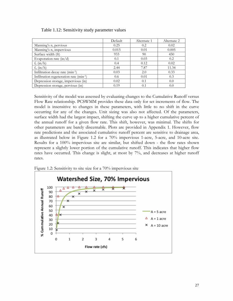
27

Table 1.12: Sensitivity study parameter values Default Alternate 1 Alternate 2 Manning’s n, pervious 0.25 0.2 0.02 Manning’s n, impervious 0.015 0.01 0.005 Surface width (ft) 933 90 450 Evaporation rate (in/d) 0.1 0.03 0.2 fc (in/h) 0.4 0.12 0.02 fo (in/h) 2.44 7.87 11.34 Infiltration decay rate (min-1) 0.03 2.0 0.33 Infiltration regeneration rate (min-1) 0.6 0.01 0.3 Depression storage, impervious (in) 0.02 0.1 0.0 Depression storage, pervious (in) 0.19 0.1 0.0 Sensitivity of the model was assessed by evaluating changes to the Cumulative Runoff versus Flow Rate relationship. PCSWMM provides these data only for set increments of flow. The model is insensitive to changes in these parameters, with little to no shift in the curve occurring for any of the changes. Unit sizing was also not affected. Of the parameters, surface width had the largest impact, shifting the curve up to a higher cumulative percent of the annual runoff for a given flow rate. This shift, however, was minimal. The shifts for other parameters are barely discernable. Plots are provided in Appendix 1. However, flow rate predictions and the associated cumulative runoff percent are sensitive to drainage area, as illustrated below in Figure 1.2 for a 70% impervious 1-acre, 5-acre, and 10-acre site. Results for a 100% impervious site are similar, but shifted down - the flow rates shown represent a slightly lower portion of the cumulative runoff. This indicates that higher flow rates have occurred. This change is slight, at most by 7%, and decreases at higher runoff rates. Figure 1.2: Sensitivity to site size for a 70% impervious site

28

Figure 1.3: Sensitivity to site size for a 100% impervious site

29

2. PCSWMM Field Studies Review WRRC was asked to evaluate the robustness of six studies used to calibrate the PCSWMM model, using the MASTEP “quality of performance data screening tool” and to the extent applicable, the EPA ETV Verification Protocol for Urban Runoff Models. The six field studies were submitted by Imbrium Systems to Massachusetts DEP in an April 28, 2008 correspondence between Daniel Nason of Imbrium and Thomas Maguire of DEP.

WRRC staff reviewed the EPA ETV Verification Protocol for Urban Runoff Models. This protocol addresses numerous features of a computer model that are not relevant to evaluation of calibration field studies. For example, requirements or recommendations are specified for such issues as user technical support, processing speed, existence of adequate documentation of version upgrades, or the presence of a user forum on product or developer’s web site. The protocol does not directly address water quality testing. It does discuss the ability of the model to accurately read precipitation records and to model hydrologic functions (e.g. evapotranspiration, channel conveyance, and pond storage and routing). Regarding precipitation records, the PCSWMM model analyzes data from long term historical rainfall data obtained from the National Climate Data Center (NCDC) of the National Oceanic and Atmospheric Administration. The ability of the model to read these data sets does not factor into an evaluation of the corroborating field studies, which (when they collected rainfall data at all) measured rainfall over typically short periods of time from local rain gauges. For these reasons, WRRC relied solely on the MASTEP quality of performance screening tool to evaluate the relevant field studies.

The MASTEP data screening tool http://www.mastep.net/database/docs.cfm#review compares field studies with required elements of a field study as established by the TARP Tier II protocol, http://www.mastep.net/documents/TARP%20Tier2protocol.doc. TARP Tier II was developed in 2001 by the member states of the Technology |Acceptance Reciprocity Partnership. The TARP Tier II protocol establishes a number of criteria to be followed in the design, conduct and reporting of performance studies of stormwater management BMPs. These criteria include, but are not limited to: number of storms, total amount of rainfall, and % of average annual local rainfall monitored; documentation of a quality assurance project plan and quality control data; documentation of test site and sampling methods; appropriate range of influent TSS concentration and particle sizes; range of flows tested; appropriate analysis methods, etc. To complete this task, the MASTEP screening tool was applied to six field studies offered by Imbrium Systems Inc., as corroboration of the PCSWMM model. WRRC staff confirmed in conversations with Imbrium that the studies were not used to calibrate PCSWMM- rather they were offered as validation of the model. Imbrium provided summary reports of the PCSWMM simulations of each of these field installations. WRRC staff examined the user-defined inputs for each of these studies, particularly sediment size distribution and presence of upstream storage. The intent of this examination was to ascertain, if possible, how closely documented conditions at each site were approximated by the PCSWMM model runs. A brief narrative summary of WRRC findings for each study is given below. This information is also provided in tabular form in the accompanying Excel table “PCSWMM Field Evaluation”(worksheet “field studies comparison”). These evaluations, revised to match the MASTEP report formats, will appear on the MASTEP web site.

30

2.1. Individual Field Performance Studies Study 1. Stormceptor Monitoring Study Como Park St. Paul Minnesota. Rinker Materials. 2002. This 2002 paper reports on a test of eight storm events from August 1998 to September 1999. Monitored storms produced a range of flow rates up to and exceeding the operating rate of the Stormceptor, and influent TSS ranging from 13 – 318 mg/l, with a flow-weighted average of 78 mg/l. The 2002 study reported that “the overall load reduction for the monitoring period was 76%”. This includes results from all eight monitored storms. This differs from the results listed in the April 28, 2008 communication from Imbrium Systems to MA DEP, which claims an 80.8% removal efficiency (sum of loads method (SOL)) for six storms, or 66.9% by event mean concentration method (EMC). The 2008 communication states that “Two [of the 8] events were removed due influent vs. effluent concentration values.” Although not specified, this is apparently a reference to the report’s mention of two storms (9/19/98 and 9/23/98) that produced low influent TSS and negative removal values (26 and 31 mg/l and -19.2% and -24.2% respectively). The exclusion of these two storms appears to be an arbitrary decision, not supported by any documentation offered by Imbrium Systems. Interestingly, the 76% load reduction cited in the original report matches the 76% efficiency simulated by PCSWMM. However, if all 8 storms are included, the Event Mean Concentration method produces 44.7% TSS removal. Note also that 3 of the events that were included had influents of 13, 23 and 48 mg/l; all had positive removal efficiencies up to 75%. It is worth noting that one of the excluded events (9/19/98) had some apparent anomalies in the flow/rain graph. High flow peaks (up to 1.6 cfs) appear prior to any significant recorded rainfall. This suggests antecedent rain that was not documented, or inaccurate flow readings. It is also possible that the graph was inadvertently reversed in the report, producing the mirror image of the intended representation. Viewed this way, the rainfall/flow relationship appears more reasonable. The 8/27/98 graph mistakenly repeats the readings from the August 7 event. Neither of these are excluded storms. This is the only study (of the six offered by Imbrium for comparison with PCSWMM) that positively documented peak flows up to and exceeding the unit’s operating rate. Two events recorded peaks of > 250% and 500% of the capacity. This is useful in evaluating the BMP and PCSWMM model performance over a full range of operating conditions. 4.6” of rainfall were monitored during the study, 14% of annual precipitation in the study area. Sampling and analysis methods were not documented. MASTEP gave this study a rating of 3: the study has some scientific merit. Significant caveats exist regarding use of the study information. In contrast to several of the PCSWMM corroboration studies offered by Imbrium, this one had no major installation or sampling problems. Nor did it test inappropriately limited flow ranges, sediments mixes, or TSS concentrations (although the latter was a little on the low side). However, this study’s lack of QC documentation and the modest number of storms evaluated (6 or 8, depending on whether storms are excluded) do not provide a robust test of the PCSWMM model. This study is one of several (five of the six studies) in which influent PSD was not reported; instead, sediments retained in the Stormceptor were analyzed for particle size and used to

31

approximate PSD for the PCSWMM model run. This approach has questionable merit, because sediments retained in flow-through units typically have a higher PSD than does influent water. If captured sediments are used to as a guide to selecting input sediments (either user-defined or by selecting from the “standard” mixes provided by the model), it would seem more logical to generate a mix with finer PSD than those found in the unit. The six mixes provided in the PCSWMM software are:

• USEPA NURP (clay, silt, sand); • NJDEP (clay, silt, sand), • Fine (organics, silt and sand); • OK-110 (sand); • F-95 (sand), and • Coarse (sand).

In this particular case none of the PCSWMM default mixes closely approximated the captured sediments - and hence the custom mix used by Imbrium in the documentation provided in a 4/28/08 correspondence with MA DEP. Of the three closest, The EPA NURP mix had more fines, the NJDEP and Fine defaults had fewer. See accompanying Excel file for PSDs of these mixes. The PCSWMM manual does not include instructions on selecting an appropriate sediment mix, other than to state “Select the particle size distribution specific to your project or local regulations”, and “Please contact your local Stormceptor Representative for assistance to use an alternative PSD not present if required for your design.” To test the sensitivity of input PSD for the PCSWMM, we ran the model for this study, using all input variables that were used in Imbrium’s 4/28/08 run except PSD. We ran it three times, using the default Fine mix, the NJDEP, and the EPA NURP mix. With the Fine and NJDEP mixes, the model runs produced a smaller recommended Stormceptor model size than that generated by Imbrium’s run. The EPA NURP mix model run produced a larger recommended model. See Como Pk PCSWMM model run reports in appendix for details. Table 2.1. Input PSD mixes, recommended STC sizes for Como Park study Model run Sediment

composition1 STC 7200 removal %

STC 4800 removal %

STC 900 removal %

Imbrium 4/28/08

User input. Approx. 5% clay, 62% silt, 33% sand

86% 82%* 72%

NJDEP default mix

5% clay , 40% silt , 55% sand

90% 88% 80%*

Fine default mix

Some organics. 0% clay, 40% silt, 60% sand

93% 91% 84%*

EPA NURP default mix

35% clay, 56% silt, 9% sand

82%* 78% 66%

1. For this table, clay is defined as < 2microns, silt as 2-50 microns, sand as > 50 to 60 microns (imprecision reflects different sizes reported in different mixes selected for the PCSWMM defaults). * = PCSWMM-recommended unit size to meet 80% TSS removal goal.

32

For the following reasons, this study has some limited value as a corroboration of the PCSWMM model: Strong points:

• The study tested a full range of flows up to and exceeding the capacity of the system. • Appropriate range of influent TSS concentration. • As reported, the study experienced no significant problems in design, sampling,

sample analysis, or data management. • Study results generally agreed with PCSWMM TSS removal estimates. (This is true of

most of the studies). Intermediate:

• Although not considered good compared to TARP sampling protocol, the study and initial report covered 8 storm events, higher than most of the other studies.

Weak points:

• Lack of quality control data. • Discrepancy between study and subsequent Imbrium-MA DEP communications

regarding number of storm events to use in calculating TSS removal efficiency. • Small amount of rainfall covered in the study. • Questionable use of sediments retained in the Stormceptor as input PSD for the

PCSWMM simulation. Study 2. Performance Assessment of Two Types of Oil and Grip Separator for Stormwater Management in Parking Lot Applications – Markham and Toronto, Ontario. Stormwater Assessment Monitoring and Performance Program. 2004. In this field study two STC 4800s were installed in parallel in the parking lot of a Home Depot store in Etobicoke, Ontario. 6.3 acres of pavement drain into the units. Parking lot runoff was distributed to the Stormceptors through an asymmetric Y-splitter: a portion of the runoff going to each unit. Because of difficulties in locating influent sampling equipment, flow was measured only at the effluent pollutant sampling location for each STC 4800, and influent TSS and other pollutants were samples downstream of the Y-splitter, upstream of the unit that was assumed to be receiving the majority of the flow. This arrangement did not allow for quantification of the relative flows through each STC 4800; report authors made an assumption that influent TSS concentrations were equal in both units. It was not possible to test this assumption. This adversely affected performance evaluation in at least two important ways. 1) Combined influent TSS concentrations reported may be incorrect, which in turn casts uncertainty on % removal efficiencies calculated by comparing influent vs. effluent concentration. 2) The operating rate of each of the 2 parallel units is unknown. It may well be that one unit was operating at a higher rate than would be normal for a storm of a particular size, while the other unit is operating at a lower than normal rate. Ability to correlate system performance with operating rate is thus lost.

33

Figure 2.1: Ontario installation monitoring set-up. (From study report)

Other factors that make this an atypical study: The unit was undersized for the drainage area. Upstream detention existed in the form of temporary storage built into the storm sewer system. The amount of storage was not quantified. This causes unknown alterations in the typical relationship between rainfall depth and intensity, runoff, and system operating rate. In addition, upstream detention is likely to provide some pre-treatment and affect particle size reaching the Stormceptor units. Study results show a mean influent particle size of 6.5 microns, well below what is typical of stormwater runoff. Collectively, these conditions are likely to adversely affect removal efficiency. Results obtained are thus likely a conservative estimate of performance of the Stormceptor. However, the inability to quantify these departures from the norm or their impacts on system performance significantly compromises the utility of this study to predict system performance in other applications. Similarly, its use in validating the PCSWMM sizing model is called into question. Rainfall data was captured in only 10 of the 16 storms monitored. Based on total volume of flow measured for each storm, it is likely that 1 to 3 storm events did not meet the minimum TARP criterion of 0.1” rain per event. Rainfall collection stations were changed part way through the study, from a site 3km away to a site 5km away. The study reports that the “volumetric runoff coefficient averaged 0.98. There were substantial variations in the runoff coefficient among individual events, suggesting possible discrepancies between the rainfall gauging stations, located 3 to 5 km away, and actual rainfall at the site. The relatively weak

34

correlation between runoff volumes and rainfall depths (R2 = 0.54) lends additional support to this hypothesis.” Flow rates of approximately 4% - 30% of operating rate were reported- however, this is based on hourly peaks. It appears from the report that at least 4 storms produced flows that briefly exceeded the operating rate. We consider this study to have produced flow ranges sufficient to test the model. However, the problems discussed above relating to the split flows render the entire data set suspect. The particle size distribution used for the PCSWMM model run approximated what was collected in the field study. Note that these are particularly fine, due no doubt to the upstream detention. The model did not incorporate any upstream storage into its inputs, although there is the opportunity to do so in the PCSWMM software. Additional study notes: The Stormceptor study is part of a study that included literature review of other stormwater BMPs ,and that compared Stormceptor performance with a non-proprietary 3-chamber Oil and Gas Separation (OGS) unit, similarly configured with 2 parallel units, installed in another Home Depot parking lot in a different suburb of Toronto. The Stormceptor study yielded average TSS influent concentration of 156 mg/l, range 30 – 634 mg/l. Approximately 6” of rainfall was monitored over the course of the study, or approximately 20% of annual precipitation occurring in the area. In addition to TSS, oil and grease, hydrocarbons and metals were sampled. Other than the problems reported above, the study appears to have been conducted according to sound methodology; however, specific analysis methods were not provided, no quality control data was included in the report, and there was no mention of a quality assurance project plan. This study received a MASTEP rating of 3: This study has some scientific merit. Significant caveats exist regarding use of the study information. For the following reasons, this study is not considered a robust corroboration of the PCSWMM model:

• the uncertain validity of TSS removal efficiencies caused by the poor design of influent/effluent and flow modeling,

• questionable flow data, resulting from flow meter placement and from suspect accuracy of rain gauges, as reported in the study report;

• unknown amount of upstream detention storage, not accounted for in the PCSWWM model run.

• abnormally fine influent sediments (due to upstream storage), creating an atypical case study.

Study 3. The Effects of Backwater on Stormceptor Treatment Systems Denver Colorado Area. Applied Hydrology Associates. 2003. This study evaluated 16 storm events. One was not monitored for TSS (equipment malfunction). Eight storm events were considered adversely affected by backwater conditions created by the downstream detention basin. Two events were rejected because of

35

inconsistent sample volumes influent vs. effluent. Three were rejected by the conducting agency because influent TSS concentrations (36, 74 and 32 mg/l respectively) were below the study’s target of 100 mg/l. This criterion is consistent with TARP requirements (as amended by NJDEP) specifying mean influent TSS of 100-300 mg/l. This leaves two events that were used to evaluate the PCSWMM. Note however that these events had rainfall 0.04” and 0.02” respectively, below the TARP criterion of 0.1”. Using only these two storms, TSS removal (EMC method) was 78.7%, which compares well with the 81% removal simulated by PCSWMM. If both criteria were enforced (100-300 mg/l mean influent and 0.1” minimum rainfall), the study would have produced no qualifying events. Two of the three storms that were not affected by backwater conditions, but which the testing agency rejected because of low influent TSS, did meet the TARP rainfall criterion (with 0.19” and 0.27” respectively). Neither of these produced flow more than approximately 25% of the operating rate of 1.77CFS for the STC 4800. These two averaged 33% TSS removal (EMC method). Thus if we reject the testing agency’s 100 mg/l influent TSS criterion and replace it with the TARP 0.1” rainfall minimum, the observed 33% TSS removal efficiency does not match well with the PCSWMM simulation of 81% removal. If all 5 storms that were not affected by backwater or sampling error were accepted (waiving both the 0.1” rainfall and 100 mg/l TSS criteria), the resulting TSS removal efficiency is 49%. Evaluating removal efficiency of these storms by Sum Of Loads method is not possible from this report, which did not document total volume of rejected storms. The total amount of rainfall monitored in the study, including backwater-affected events, was < 3”. Although study methods were well documented and apparently carried out well, and good QC data was reported, problems with the backwater left insufficient data to allow a useful evaluation of the system’s performance. This study received a MASTEP rating of 3: This study has some scientific merit. Significant caveats exist regarding use of the study information. MASTEP considers the study’s comparison of modeled performance efficiency (via PCSWMM) vs. actual performance to be invalid for these reasons:

• Two storms that were used to compare with PCSWMM were too small to qualify, using TARP criterion of minimum 0.1” storm depth.

• Two storms that were excluded by study agency but which did produce > 0.1” rain produced very different results from PCSWMM (33% vs. 80%)

• The study’s SOP called for measuring only TSS 100mgl/ or higher. This seems to have biased results in favor of higher removal efficiencies.

• The overriding concern is an insufficient number of data points and an inadequate range of conditions (flow, TSS level, documented particle size (no PSD analysis done) to produce a valid comparison.

Study 4. Urban Runoff Pollution Mitigation Study. The Phoenix Group. Edmonton Alberta. 1996. This field study of a Stormceptor 2400 monitored 4 events. TSS, COD, and metals were monitored. Little or no information is provided on total rainfall monitored, flow rates into unit, sampling/analysis methods, or quality control. Influent TSS concentrations ranged

36

from 159-1058mg/l, average 405. No information was given on influent particle size. The unit was significantly undersized for the drainage area of 9.9 acres, one factor contributing to a relatively low TSS removal efficiency of 51.5% (EMC method). Although there were no obvious errors in methods or study approach found, the report offers insufficient information and the study monitored too few events to provide a robust evaluation of the system's performance. This study received a MASTEP rating of 3: The study has some scientific merit. Significant caveats exist regarding use of the study information. This study was a follow-up to one conducted the previous year, using the same Stormceptor unit that was configured slightly differently. At the end of the earlier study, sediment samples captured in the unit were analyzed for grain size. The particle size distribution found in the unit was mimicked when the PCSWMM simulation was run. We question this approach; it likely produces a bias toward larger particle sizes, as discussed in the Como Park MN study section. The study did test a appropriately wide range of TSS concentration. Based on watershed to STC unit size ratio, it provided a test of system performance under extreme conditions. Methods followed appear to be sound. The small number of storms monitored, lack of rainfall or flow data, and lack of detail on methods and quality control limit the value of this study as a corroboration of the PCSWMM model.

Study 5. SeaTac Stormceptor Performance Monitoring Report. Associated Earth Sciences, Inc. Kirkland Washington. 2001. This field study evaluated a Stormceptor STC 900 that drained a 1 acre impervious convenience store parking lot and driveway. 4 storms totaling 1.45” of rain were monitored, or 3.9% of annual average rainfall in the area. Peak flows into the Stormceptor ranged from approximately 0.01 CFS to 0.04 CFS, or approximately 1.6% to 6.4% of the unit’s 0.63CFS operating rate. A detention chamber (no specifics given on size, configuration) and flow splitter immediately upgradient of the Stormceptor diverted flow during the first 3 storms, resulting in lower than expected discharge to the Stormceptor. The PCSWMM model allows user-defined site configuration inputs that would account for upstream detention. However when the PCSWMM simulation provided by Imbrium for this site was run, this option was not used. This would likely produce changes in influent flows, PSD and TSS concentration that the model would not account for. The study noted discrepancies between inflow and outflow discharge measurements: “The apparent sensor discrepancies may have been caused by debris clogging the inflow sensor”. The report provides few details on site characteristics and sampling methods. Analysis was conducted at a certified lab. Detailed laboratory data was provided, including quality control data. The small number of storms, minimal precipitation and low flows monitored, the lack of detail on methods, and the problems encountered with flow measurements limit the ability

37

of this study to produce a meaningful evaluation of the Stormceptor’s performance. This study received a MASTEP rating of 3: The study has some scientific merit. Significant caveats exist regarding use of the study information. Particle size analysis was done after monitoring had been concluded, by collecting sediment samples from the inlet and outlet of the upstream detention chamber and from the Stormceptor forebay . The report provides PSD results, but it is unclear which of the sediment samples are represented in the PSD report (i.e. inlet, outlet, or chamber floor?). The PCSWMM modeling exercise used particle size distributions that mimic those in the report, variously labeled “SeaTac outflow” or “Stormceptor outflow”. This confusion inhibits our ability to evaluate the validity of the PSD inputs to the model. The report states that “accurate discharge events were difficult to obtain during several of the storm events”. This calls into question the data used for Sum Of Loads comparison with PSCWMM. For these several reasons: few storms and small amount of precipitation monitored, low flow ranges tested, possible errors in flow measurements, failure to account for upstream detention, and confusion over PSD reported render this study of limited value in evaluating the PSCWMM. Study 6. Field Evaluation of a Stormceptor Model STC 1200 Westwood, MA. Stormceptor Group of Companies. 2004. This field study of a Stormceptor STC 1200 monitored 5 storms, only 4 of which were used for performance evaluation. (Storm #4 produced TSS influent and effluent below detection limit). TSS, TPH and metals were monitored. Scant information was provided on site layout, test setup. Limited information is provided on methods. Study approach and methodology appeared to be sound. Only 1.5" total rainfall was monitored during the study (3% of annual precipitation in Westwood MA); flows tested were very low compared to the operating rate of system (peak flows < 3% of design). The study reports that an unusual amount of coarse material was collected by this unit: “approximately 50% of the material being classified as fine gravel.” 27% of the material was finer than 60 microns. No analysis of influent sediment size distribution was reported. This study does not provide sufficient information to allow a robust evaluation of the Stormceptor's performance over a range of conditions. This study received a MASTEP rating of 3: The study has some scientific merit. Significant caveats exist regarding use of the study information. As with several other of the studies used to corroborate PCSWMM, the sediment mix input to the model mimicked sediments found in the chamber, rather than PSD measured from influent water samples. We question this approach; it likely produces a bias toward larger particle sizes, as discussed in the Como Park MN study section. The small number of storms, low flows, limited documentation of methods, the atypical sediment size and questionable method of inputting sediment sizes to the PCSWMM model all render this study suspect as a corroboration of the model.

38

2.2. Influent Particle Size Discussion. To further examine the influence of particle size distribution on PCSWMM simulation outcomes, we ran several simulations for each of the six installations, using a variety of PSDs as the input parameter for each, with all other parameters remaining constant for each installation. PSCWMM output summary files for each of these simulations are available as separate files. The accompanying Excel file (worksheet “PSD trials”) summarizes the results. Similar to what is displayed in Table 2.1 above, the summary results illustrate that for a given site and Stormceptor unit size, predicted removal rates can vary by 15% to 20% or more, depending on input sediment mix. Using an 80% removal target, the recommended STC model can vary by as much as three or four unit sizes. For instance, PCSWMM recommended an STC 450i for the SeaTac installation (with predicted 90% removal) with the user-defined input sediment mix (provided by Imbrium in this case); using the EPA NURP mix instead, the recommended unit would be an STC 4800 (with 83% removal), three unit sizes larger. From these results, it is apparent that influent sediment size significantly influences Stormceptor sizing with PCSWMM. Given this significance, if any future attempts are made to corroborate or calibrate PCSWMM results with those from field installations, it will be important to resolve the question raised earlier in this memo regarding use of captured sediments as the input mix. It would seem more appropriate to use a finer mix than what is found in a unit. The PCSWMM manual provides little instruction on selecting particle size mix for the simulation input: “Step 5 allows the user to choose the desired particle size distribution (PSD) to define total suspended solids (TSS). The user can select from five (5) pre-set distributions. In addition, a grain size plot illustrating the five (5) particle size distributions is available by clicking the Graph PSDs button. The Fine particle distribution is the default distribution. Please contact your local Stormceptor® Representative for assistance to use an alternative PSD not present if required for your design.” (PCSWMM manual, ,P 16) We recommend that this documentation be expanded to provide more detailed guidance to PCSWMM users on how to select input sediment mixes. 2.3. Influence of rainfall and flows on system performance, field studies vs. PCSWMM. At the request of DEP, WRRC investigated the question of how PSCWMM output compares with the field studies at different flow rates. It is possible to view PCSWMM single-day hydrographs based on a given rainfall input. This can be done in the TM version by opening the “view hydrograph” menu item in the “Step 9 – Design Summary” page and zooming in to the dates of interest. The same can be done for rainfall data via the “view rainfall” selection. However, PSCWMM pre-set inputs are limited to pre-loaded data sets obtained from the U.S. Department of Commerce, National Oceanic Atmospheric Administration (NOAA), EarthInfo, Inc, Environment Canada, or certain various local municipalities. PCSWMM does allow users to input different rainfall data sets, but the

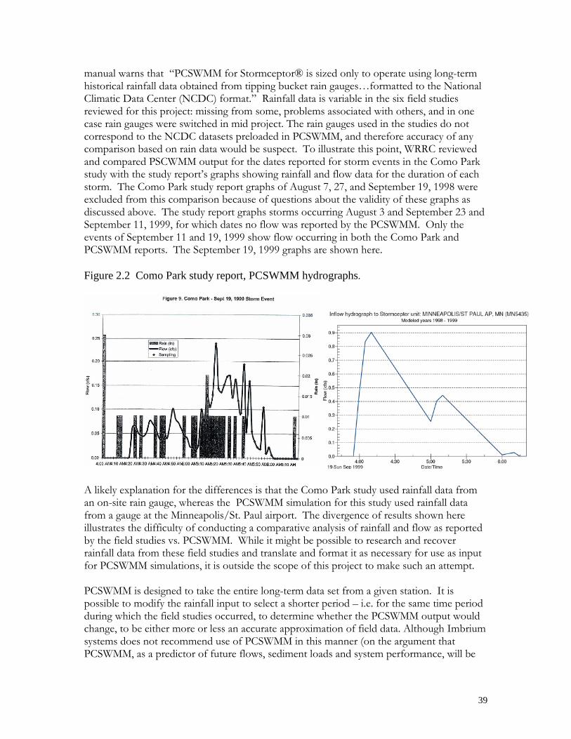
39

manual warns that “PCSWMM for Stormceptor® is sized only to operate using long-term historical rainfall data obtained from tipping bucket rain gauges…formatted to the National Climatic Data Center (NCDC) format.” Rainfall data is variable in the six field studies reviewed for this project: missing from some, problems associated with others, and in one case rain gauges were switched in mid project. The rain gauges used in the studies do not correspond to the NCDC datasets preloaded in PCSWMM, and therefore accuracy of any comparison based on rain data would be suspect. To illustrate this point, WRRC reviewed and compared PSCWMM output for the dates reported for storm events in the Como Park study with the study report’s graphs showing rainfall and flow data for the duration of each storm. The Como Park study report graphs of August 7, 27, and September 19, 1998 were excluded from this comparison because of questions about the validity of these graphs as discussed above. The study report graphs storms occurring August 3 and September 23 and September 11, 1999, for which dates no flow was reported by the PCSWMM. Only the events of September 11 and 19, 1999 show flow occurring in both the Como Park and PCSWMM reports. The September 19, 1999 graphs are shown here. Figure 2.2 Como Park study report, PCSWMM hydrographs. A likely explanation for the differences is that the Como Park study used rainfall data from an on-site rain gauge, whereas the PCSWMM simulation for this study used rainfall data from a gauge at the Minneapolis/St. Paul airport. The divergence of results shown here illustrates the difficulty of conducting a comparative analysis of rainfall and flow as reported by the field studies vs. PCSWMM. While it might be possible to research and recover rainfall data from these field studies and translate and format it as necessary for use as input for PCSWMM simulations, it is outside the scope of this project to make such an attempt. PCSWMM is designed to take the entire long-term data set from a given station. It is possible to modify the rainfall input to select a shorter period – i.e. for the same time period during which the field studies occurred, to determine whether the PCSWMM output would change, to be either more or less an accurate approximation of field data. Although Imbrium systems does not recommend use of PCSWMM in this manner (on the argument that PCSWMM, as a predictor of future flows, sediment loads and system performance, will be

40

most accurate with the most complete data set possible), MASTEP staff did run simulations for the Edmonton, Toronto and Como Park data sets, using all parameters identical to the PCSWMM run (including user-input sediment distribution) provided by Imbrium in the April 28, 2008, except rainfall record period. For this, the two years containing the respective study periods were chosen, rather than the full rainfall records of seven years (Edmonton), 18 years (Toronto) and 58 years (Como Park) respectively. 15. PSCWMM does not allow user-input rainfall record years of finer resolution than one year. The Toronto and Edmonton runs produced identical results to the full-period PCSWMM simulation provided by Imbrium. The Como Park short term simulation differed from the full-duration simulation by modest amounts (0% to 3%) for different STC unit sizes, as seen in the table below. Table 2.2. Input PSD mixes, removal efficiencies (recommended STC unit size in bold)

Como Park - STC 1800 PCSWWM Results by STC model

1948-2005 rainfall data

1998-99 rainfall

STC 450i 63% 65% STC 900 72% 74% STC 1200 72% 74% STC 1800 73% 75% STC 2400 77% 79% STC 3600 79% 80% STC 4800 82% 84% STC 6000 83% 84% STC 7200 86% 87% STC 11000 89% 90% STC 13000 90% 90% STC 16000 91% 92%

2.3. Field Studies Review - Conclusions All of the studies had one or more significant problems sufficient to earn a MASTEP rating of 3. Although none of the field studies significantly contradicted the TSS removal efficiencies predicted by the model, nor did any single study provide a strong validation of the PSCWMM model. All suffered from some combination of low flows, small number of storms, small amount of rainfall monitored, inadequate documentation of methods or quality control, and errors in installation and/or sampling methods. One might argue that collectively, the studies offer a sufficient body of evidence (e.g. number of storm events, rainfall totals, varying flow rates etc.) to validate the model, but it is the opinion of WRRC staff that this argument has flaws. The studies did not follow, nor document, a uniform set of standard operating procedures that would justify aggregating results from the several studies. Even if consistency of methods were assumed, the documented problems (e.g. frequent backwater conditions in one study, unreliable flow measurements in another, missing rainfall data in a third) significantly reduce the number of data points suitable for comparison with PSCWMMM outputs. The six studies provided do not constitute a

41

rigorous test of PCSWMM’s ability to predict TSS removal efficiency, nor of the adequacy of the PSCWMM to convert Water Quality Volume to a flow rate. Individually, the two studies that provide the strongest validation of the PCSWMM are, in descending order, the Como Park, Minnesota study and the Edmonton, Alberta study. The study reports referred to in this memo are:

o Urban Runoff Pollution Mitigation Study. The Phoenix Group. Edmonton Alberta. 1996.

o Performance Assessment of Two Types of Oil and Grip Separator for Stormwater Management in Parking Lot Applications – Markham and Toronto, Ontario. Stormwater Assessment Monitoring and Performance Program. 2004.

o SeaTac Stormceptor Performance Monitoring Report. Associated Earth Sciences, Inc. Kirkland Washington. 2001.

o Stormceptor Monitoring Study Como Park St. Paul Minnesota. Rinker Materials. 2002.

o Field Evaluation of a Stormceptor Model STC 1200 Westwood, MA. Stormceptor Group of Companies. 2004.

o The Effects of Backwater on Stormceptor Treatment Systems Denver Colorado Area. Applied Hydrology Associates. 2003.

42

3. Alternative Method Evaluation WRRC was asked to evaluate the adequacy of the Ahlfeld, Bryant, and Claytor methods using the same criteria applied to the PCSWMM in section 1 above. It should be noted that these alternative methods do not account for snowfall. Within the analyses, precipitation falling during the winter is treated analogously to that in other seasons. Runoff volume is typically considered to be the most important hydrologic variable for water quality protection while runoff peak rate is more important for drainage system design and flood prevention. As a result, most states base sizing guidelines on the volume of runoff to be filtered on an event basis, assuming that this sizing will result in the treatment of a minimum percentage of the annual runoff volume (e.g., 90% of the average annual runoff). While methods for determining the appropriate runoff volume for treatment vary, local rainfall volume and rate data are important deterministic factors. Most methods convert rainfall to runoff through either an empirical or physically based equation and assess the appropriate treatment volume based on a frequency distribution. Some BMP sizing and performance evaluation methodologies, however, are based on runoff rate rather than volume, requiring conversion of the runoff volume to be treated to a peak rate of discharge the system must be designed to treat. This document examines the procedures utilized by three methods to identify the Water Quality Volume (WQV) to be treated and convert this volume to a peak rate for treatment. 3.1. Ahlfeld Method Background

The initial underlying premise of the Ahlfeld method was that for small, highly impervious sites there is a 1:1 translation of rainfall to runoff (Winkler et al, 2001). This premise was later altered through use of the rational method to convert rainfall intensity associated with the first-flush volume of a storm to peak flow (Ahlfeld, 2004). The focus of the method is the development of intensity-frequency relationships for the first-flush average and maximum rainfall intensities. It should be noted that these curves differ from traditional intensity-duration-frequency curves developed based on the complete rainfall record. Ahlfeld analyzed 15-minute precipitation data from 20 Massachusetts stations on an event basis with storm events defined using both a 1-day and a 3-day interstorm period. Regional characteristics were assessed based on the number of storms observed during the period of record at each station. Several stations were discarded from the analysis based on period of record or heterogeneity in comparison to the other stations. In the end, two distinct homogeneous regional groups were identified for further analysis, coastal and mainland east of the Berkshire Mountain range. Originally (Winkler et al., 2001) the mainland group contained 11 stations and the Cape Cod or Coastal group contained 3 stations. Later these groups were reduced to five and two stations, respectively, based on more rigorous evaluation (Ahlfeld et al, 2004). The resulting storm event data for each region were lumped to develop intensity-frequency curves for two rainfall depth accumulations, 0.5 and 1.0 inches. Three intensity-frequency relationships were developed for each region based only on rainfall intensities during the first flush portion of the storm:

43

1. Average intensity until 0.5” of precipitation is reached, 1-day interstorm period (Winkler et al., 2001 only),

2. Maximum intensity occurring before 0.5” of precipitation is reached, 1-day interstorm period,

3. Maximum intensity occurring before 0.5” of precipitation is reached, 3-day interstorm period (Ahlfeld et al., 2004 only),

4. Average intensity until 1.0” of precipitation is reached, 1-day interstorm period (Winkler et al., 2001 only),

5. Maximum intensity occurring before 1.0” of precipitation is reached, 1-day interstorm period,

6. Maximum intensity occurring before 1.0” of precipitation is reached, 3-day interstorm period (Ahlfeld et al., 2004 only),

Events where the specific rainfall depth was not achieved were omitted from the analysis. Events which exceeded the rainfall depth were included, but only intensities prior to the 0.5 or 1.0 inch accumulation were evaluated. Cumulative frequency distributions were generated for each classification by grouping the resulting intensities in bin intervals. For the average intensity results, interval widths of 0.4 in/hr were used. For the maximum intensity results, interval widths of both 0.4 and 0.2 in/hr were used, however the analysis procedures associated with the 0.2 in/hr interval width are more rigorous. The methods utilized to convert the resulting histograms to a frequency in the Winkler et al. (2001) method are not fully described, but were likely based on a simple plotting position technique (e.g., divide number of occurrences in bin by total number and utilize these probabilities to generate the cumulative frequency). Results are summarized graphically as cumulative frequency of occurrence versus intensity. The Ahlfeld et al. (2004) paper formally determines the probability density function and utilizes this distribution to determine the maximum rainfall intensity associated with the two WQVs, regions, and interstorm periods. Maximum intensity results are tabulated for four return periods (0.25, 0.5, 1, and 2 years), calculated for specifically for the partial duration series. Discussion The Ahlfeld method focuses on rainfall rates occurring prior to attainment of the runoff volume and utilizes these values to assess frequency of occurrence or return period. A single value for each event is utilized, either the maximum or average rainfall rate in the period leading up to attainment of the WQV. The method is thus based on a subset of the 15-minute precipitation rate data; this partial duration series is defined based on precipitation accumulation. All seasons are included in the analysis and precipitation is assumed to be in the form of rain (rather than snowfall). It is important to note that the development of the partial duration series results in significant reduction in the amount of the data used for analysis. For example, the period of record for Hyannis extends from January 1984 to May 1997. While the actual number is significantly less due to no-rain and missing data time periods, the 14+-year time period potentially includes over a half-million rainfall rate values. The number of storms for this station based on a 1-day interstorm period is 849 and for a 3-day interstorm period only 539. This data set is further reduced to include only those that meet the WQV criteria of 0.5 or 1.0-inch. The Ahlfeld methods are based on the data set consisting of a single rainfall rate value for each event. Thus the number of data points utilized in the analysis is reduced by approximately 3 orders of magnitude.

44

Based on the result of the analysis, the user can then select a rainfall rate that meets a predefined criterion and utilize this to infer the peak rate of treatment based on the Rational Method. The method differs from the traditional application of the Rational Method, which selects rainfall intensity from a standard intensity-duration-frequency curve based on time of concentration (and the full period of record of data). No information on time of concentration is required for the Ahlfeld method. In addition, no guidance is given in terms of identifying appropriate runoff coefficients. It is unclear what impact this has on the ultimate accuracy of the runoff rate prediction. While not as rigorous in methodology, the frequency diagrams presented in Winkler et al. (2001) can be used for selecting a rainfall intensity to be translated to a peak runoff rate for treatment. The return period, utilized to present results in Ahlfeld et al. (2004), for a partial duration series cannot be directly used to infer exceedence probability, as it rather reflects the average interval between events. However, this value is attainable from the underlying distribution with parameters as published in the paper. Because a unique distribution is derived for each combination (e.g., 3-day inter storm period and 0.5-inch WQV), a given rain rate will have a different cumulative density function value based on the storm assumptions used to define the data set. In addition, a set storm precipitation accumulation is used to define the partial duration series for both methods. However the data actually utilized for analysis is the maximum intensity in the period leading up to attainment of that depth. There is thus a disconnect between the actual frequency of occurrence associated with a given rainfall rate and that defined by the method. In addition, the two-step process does not fully meet the traditional definition of a partial duration series. While this was done purposely, its impact should be considered. As noted above, the rainfall intensity data set utilized in the frequency analysis is reduced from over 100,000 data points per station (which are then combined by region) to around 200 (1” storms) or 600 (0.5” storms) per station. The meaning of the resulting frequencies becomes nebulous. It is unclear what frequency level is most appropriate for design. Storm events for the method are defined based on attainment of either 0.5 or 1.0 inches of rainfall. However, for most watersheds, the precipitation amount that translates into a runoff volume of 0.5 or 1.0 inch will actually be greater due to losses and attenuation. The Ahlfeld method does not try to identify the precipitation depth that results in 0.5 or 1.0 inches of runoff. To account for losses, the precipitation depths utilized in the evaluation should be larger, however this shift will be dependent on location and antecedent conditions.

Summary The method incorporates an extensive and thorough review of the raw precipitation

data used as the basis of the method development. The original method assumed a 1:1 translation of rainfall rate to runoff rate, noting

this was a conservative assumption. In the 2004 paper, use of the rational method is suggested to translate the peak. This is likely a conservative assumption, although it does not account for the potential for concentrated flows to result in higher runoff rates.

45

The method uses an alternative definition of rainfall intensity to define peak runoff rate via the Rational Method. It is unclear what impact this has on the ultimate accuracy of the runoff rate prediction.

The methodology results in a significantly truncated data record which is utilized as the basis of analysis. The impact on the flow estimation is unclear, but the frequency at which high rainfall rates occur is likely underestimated as a result.

There is a disconnect between the actual frequency of occurrence associated with a given rainfall rate and that defined by the method. The meaning of the resulting frequencies becomes nebulous. It is unclear what frequency level is most appropriate for design.

The method does not try to identify the precipitation depth that results in 0.5 or 1.0 inches of runoff but assumes a 1:1 translation. To account for losses, the precipitation depths utilized in the evaluation should be larger, however this shift will be dependent on location and antecedent conditions. The assumption that rainfall depth is equivalent to runoff depth is likely not conservative.

The underlying rainfall data utilized in the analysis appear appropriate for the regions specified. While it is reasonable to lump the data by region to provide a larger data set for analysis, the underlying spatial variability is of interest. More information on the rainfall rates of individual stations is of interest.

While not as rigorous in methodology, the frequency diagrams presented in Winkler et al. (2001) are useful for selecting a rainfall intensity to be translated to a peak runoff rate for treatment.

The Winkler (2001) results for average rainfall intensity prior to attainment of the WQV result in lower estimates of flow rate than likely occur and is not recommended.

3.2. Bryant Method Background As for the Ahlfeld method, the underlying premise of the Bryant method is that for small, highly impervious sites there is a 1:1 translation of rainfall to runoff. Based on this premise, annual rainfall depth cumulative frequency distributions as a function of rain rate may be utilized to directly translate a percentage of the average annual rainfall volume (ergo runoff volume) to be treated into a rainfall rate (ergo runoff rate) that a treatment devise must effectively treat. The results are independent of drainage area, infiltration and evaporation rates, depression storage, and runoff equation parameters. It should be noted that while Bryant includes a sensitivity study on the effect of initial abstraction (a portion of depression storage), ultimately no accounting for initial abstraction or other elements of depression storage is applied. The Bryant method will tend to maximize runoff volumes and rates; the potential for over-estimation will increase as percent imperviousness decreases and site area, depression storage, and other losses increase. Rather than converting the Water Quality Volume of 1-inch or ½ inch to a flow rate, the Bryant method assesses the cumulative annual runoff volume as a function of rainfall rate; the appropriate flow rate for treatment is associated with the desired percentage of the annual runoff to be treated, as described above. Direct evaluation of cumulative runoff is accomplished through a continuous simulation of runoff over the period of record at the

46

temporal resolution of the available rainfall data. For every year in the period of record, an annual cumulative distribution curve for rainfall (ergo runoff) total depth is calculated based on the observed rainfall intensities. The full available 15-minute precipitation record is utilized in the analysis; no storm inter-period or accumulation depth is defined. Only the stations deemed acceptable by Ahlfeld (2004) are included. As previously noted, rainfall intensity is assumed to be directly correlated with runoff flow rate. The cumulative frequency curves for individual years are used to develop an average annual curve for a given station. Bryant developed average annual cumulative distribution curves for 11 Massachusetts mainland NCDC stations. The resulting average curves for each station were then utilized to develop the single curve for the Massachusetts mainland and associated confidence intervals. Discussion Across the Massachusetts mainland, Bryant’s results suggest that there is a wide range of rainfall (runoff) rates associated with a given percentage of annual rainfall (runoff) depth. For example, 80% of the runoff occurs at rates ranging from 0.4 to 0.7 in/h while 95% of the runoff occurs at rates ranging from 1.25 to 2.4 in/h. The data from the various stations are utilized to present a mean and upper and lower confidence limits. Because of the spatial variability, it may be more appropriate in design to utilize the cumulative frequency curve nearest the site where a sufficient rainfall record is available, developing confidence intervals specific for the specific rain gauge location from the annual variability contained within the period of record. The accuracy of the method is highly dictated by the underlying rainfall data. The Bryant Method utilizes the same mainland Massachusetts’s rainfall data as the Winkler/Ahlfeld method, discussed above. These data have a minimum 15-minute resolution of 0.1 inches, which translates into a minimum rainfall intensity of 0.4 in/hr. The analysis is thus dependent on the reasonableness of the assumption that the critical minimum rainfall rates for treatment are greater than this value. The accuracy of the method is most dependent on the assumption that rainfall volume and rate are directly (1:1) correlated with runoff volume and rate. The validity of this assumption is greater for small areas that are 100% impervious. However, even for small sites that are 100% impervious, some losses are expected due to depression storage, flash evaporation, infiltration through cracks and seams, interception of rainfall by over-hanging vegetation, and sorption. In addition, some runoff rate attenuation may occur or, conversely, the shape of the area may concentrate flow in such a way that the runoff peak is amplified. The Bryant method does not account for any losses, attenuation, or flow path impacts. The Bryant method will typically maximize runoff volumes and rates; the potential for over-estimation will increase as percent imperviousness decreases and site area and potential losses increase. In some ways, however, the method avoids the subjectivity associated with the requirement to treat the 1-inch or ½ inch Water Quality Volume. Rather than assuming a priori what typical event runoff volume is associated with a given percent of the annual runoff, this value is directly calculated based on historical rainfall volume and rate data. A direct calculation such as this is desirable if the accuracy of the underlying runoff rate and volume estimates is acceptable.

Summary

47

The accuracy of the method is highly dependent on the assumption that rainfall volume and rate are directly (1:1) correlated with runoff volume and rate. o The Bryant method will tend to maximize runoff volumes and rates; the potential for

over-estimation will increase as percent imperviousness decreases and site area increases.

o Rather than assuming a priori what typical event runoff volume is associated with a given percent of the annual runoff, this value is directly calculated based on runoff volume and rate estimates. A direct calculation such as this is preferential if the accuracy of the underlying runoff rates and volumes is acceptable.

The accuracy of the Bryant method is highly dictated by the underlying rainfall data. o These data have a minimum 15-minute resolution of 0.1 inches, which translates into

a minimum rainfall intensity of 0.4 in/hr. The analysis is thus dependent on the reasonableness of the assumption that the critical minimum rainfall rates for treatment are greater than this value.

o Because of station-to-station variability, it may be more appropriate in design to utilize the Bryant cumulative frequency curve for the location nearest the design site, developing confidence intervals specific for the specific rain gauge location from the annual variability contained within the period of record.

o The underlying rainfall data appear appropriate for the region specified. 3.3. Claytor Method Background The Claytor method utilizes the rainfall frequency spectrum (RFS) to determine the appropriate rainfall volume to be treated. In contrast to the frequency distribution calculated for the Bryant method, the Claytor method RFS relates event rainfall volume (inches) to the recurrence interval (years). In order to develop a RFS curve, first rainfall data for the period of record at a representative station is converted to event rainfall depth. The recurrence interval (inverse of the exceedence probability) associated with various depth classes is then determined. Accumulations less than 0.1 inches are omitted from the frequency analysis. This curve and the underlying data are then utilized to determine the rainfall volume and return interval associated with various percentages of observed storm events (e.g., 90% of all storms have a rainfall volume of <1.25 inches and an associated return interval of 3 months). Claytor applied the RFS in the Washington D.C. area based on 50 years of hourly rainfall data, with individual events separated by at least 3 hours of no-rain. The cumulative rainfall volume for water treatment is thus converted to an event storm rainfall volume to be treated based on the RFS curve. For the D.C. and Chesapeake Bay area, Claytor suggests that a one-inch rainfall criterion is appropriate. The WQV is estimated from the precipitation depth to be treated based on a modified SCS TR-55 method. The modification is designed to avoid under-prediction of runoff volumes (noted in the literature) by the SCS method during smaller but more common events occurring in small drainage areas, particularly those where urbanization has decreased the infiltration capacity of pervious surfaces. Two alternative conversion methods are suggested, the Short Cut Method and the Small Storm Hydrology Method. Both methods use a runoff coefficient (analogous to the C value for the rational method and the CN value for the SCS method) in the calculation but increase the value of this coefficient relative to other

48

methods, thus resulting in a higher fraction of the precipitation resulting in runoff. The Short Cut Method utilizes equations 1 and 2 below:

WQV = PtRv (1)

Rv = 0.05 + 0.009I (2) where WQV is the Water Quality Volume to be treated in inches, Pt is the rainfall depth to be treated as determined by prior analysis, Rv is the volumetric runoff coefficient, and I is the site percent imperviousness. The WQV can be converted to a volume by multiplying by the watershed area and applying the appropriate unit conversions. In contrast, for the Small Storm Hydrology Method, equation (1) is again utilized, but the runoff coefficient Rv is determined from tabulated values that vary by Pt as well as site characteristics, including rough land-use characteristics, soils, and the level of connectivity between pervious and impervious areas. The Rv values were adapted from work by Pitt (1994). The resulting WQVs for both methods are designed to better capture small storm hydrology response as observed by the author and others. For treatments that require sizing based on a flow rate, the Claytor method converts the resulting WQV to a peak discharge based on the SCS TR-55 Graphical Peak Discharge Method, Equation 3.

qp = quAQWQV (3) where qp is the peak discharge in cfs, qu is the unit peak discharge in cfs/mi2/inch (tabulated graphically as a function of the ratio of initial abstraction to rainfall versus the time of concentration), A is the drainage area in square miles, and QWQV is the water quality volume in inches. The only deviation from the standard method is that the CN value used to determine the Initial Abstraction, Ia, is back calculated from the WQV, Equation 4, derived from the SCS methods for estimating runoff depth and retention storage:

CN =1000

10 + 5Pt +10QWQV −10(QWQV2 +1.25QWQV Pt )

0.5 (4)

Discussion The utilization of a RFS to determine the appropriate rainfall volume to be treated (Pt) based on a percentage goal is reasonable. However, rainfall characteristics will vary regionally, thus the 1.0” rainfall event criterion for sizing storm water devices may not correspond with the treatment of 90% of the annual average rainfall events in Massachusetts. Regional data should be evaluated in an analogous manner to assess the appropriate rainfall volume to be treated for the Massachusetts mainland and coastal areas, as well as to determine if further spatial variations need to be taken into account. The Claytor methodology for conversion of the Pt to a WQV appears reasonable. The method is analogous in varying degrees to both the Rational and SCS method. In the Rational Method, a runoff coefficient (or percentage of rainfall resulting in runoff) is applied to rainfall rate rather than volume. In the SCS method, the CN is used to assess the amount

49

of retention and initial abstraction available in the watershed and this is related to runoff volume through a conceptual relationship. The Claytor method is thus more aligned with the Rational Method (runoff volume is a simple percentage of the rainfall). The Claytor method estimates the appropriate runoff coefficient either through Equation 2 or via a weighted value calculated from method specific tabulated coefficients. Both methods were developed to better simulate observed responses of small watersheds to the size of events most relevant to water quality treatment. These adjustments seem reasonable and well founded. The SCS TR-55 Graphical Peak Discharge method, utilized by Claytor for conversion of the WQV to a runoff rate (qp), is a widely accepted methodology. The accuracy of the method will depend in part on the accuracy of the time of concentration estimate for the basin. The smallest time of concentration for which unit peak discharge data is available is 6 minutes. The unit peak discharge rate selected is likely more sensitive to rainfall type (Type I, II, or III) than time of concentration. The Type III distribution should be utilized for Massachusetts. The method is also sensitive to the ratio of the initial abstraction to precipitation. In order to account for the greater sensitivity of small watersheds to smaller events, noted above, the initial abstraction is back calculated from the Claytor method estimate of WQV. It should be noted, however, that the SCS method typically utilizes the 24-hour rainfall depth for a given recurrence interval which is typically 2-years or more. The Claytor method substitutes in the rainfall depth to be treated, which may or may not correspond to a 24-hour rainfall. It is unclear what impact the focus on more frequent events (< 2 year return interval) and different durations may have on accuracy of the SCS TR-55 Graphical Peak Discharge Method. In general, 2-years was utilized in the SCS method development as this return period typically is associated with bank flow conditions.

Summary The utilization of a RFS to determine the appropriate rainfall volume to be treated

(Pt) based on a percentage goal is reasonable. However, regional data should be evaluated in an analogous manner to assess the appropriate rainfall volume to be treated for the Massachusetts mainland and coastal areas, as well as to determine if further spatial variations need to be taken into account.

The Claytor methodology for conversion of the Pt to a WQV appears reasonable. In particular, the adjustments to the runoff coefficient to better simulate observed responses of small watersheds to the size of events most relevant to water quality treatment are reasonable and well founded.

The SCS TR-55 Graphical Peak Discharge method, utilized by Claytor for conversion of the WQV to a runoff rate (qp), is a widely accepted methodology.

It is unclear what impact the utilization for more frequent events (< 2 year return interval) and different durations (< 24 hours) may have on accuracy of the SCS TR-55 Graphical Peak Discharge Method.

The accuracy of the conversion from a WQV to a peak runoff rate will depend in part on the accuracy of the time of concentration estimate for the basin.

3.4 Alternative Methods Overall Discussion and Summary Three methods for converting a WQV to a peak runoff rate were reviewed in order to evaluate their adequacy. These methods have few underlying parameters, thus the review

50

mainly focused on reasonableness of the underlying assumptions and appropriateness to represent Massachusetts conditions. This section provides an overview of the relative strengths and weaknesses of the three methods. Of the three methods, the Claytor method provides the most thorough evaluation of basin runoff response to rainfall inputs. In particular, Claytor provides a methodology for assessing the storm event precipitation depth that results in treatment of 90% of the annual average rainfall. This storm depth is then translated to a runoff volume and rate in a manner designed to replicate field studies specific to small storms and small sites. While the underlying data to support this methodology is not provided for a thorough assessment, the underlying assumptions and reasoning are sound. To convert WQV to runoff rate, the method utilizes the SCS TR-55 Graphical Peak Discharge method. This method is typically applied for rainfall accumulations over 24 hours and with return periods greater than 2 years. The impact of the application for shorter time periods (for instance, in cases where the WQV accumulates in time periods less than a day) on accuracy of the peak discharge rate is unclear. It is possible that the SCS TR-55 unit peak discharges underestimate peaks for smaller events and smaller areas in an analogous fashion to that described for underestimation of runoff volume. The Claytor analysis of WQV is not specific to Massachusetts, however, which is the major limitation of the method. The Ahlfeld and Bryant methodologies are very similar, but distinct in two important aspects. The Bryant method utilizes the full rainfall intensity record in its frequency estimation. Rather than determining a WQV that will result in treatment of a specified volume of the annual precipitation, the method directly relates cumulative precipitation to rainfall rate. It makes no distinction on an event basis. In contrast, the Ahlfeld method truncates this data set to one rainfall intensity per event, and only those events which achieve the WQV for treatment (assumed to be equivalent to the precipitation depth) are included in the analysis. The reduction in the rainfall time series utilized by the Ahlfeld method raises some concerns, as does the definition of storm depth utilized. In contrast, the Bryant method assumes a 1:1 correlation between rainfall and runoff rate. The Bryant method will likely overestimate runoff rate while the Ahlfeld method ignores losses in its utilization of the WQV as a storm depth but subsequently accounts for losses in translation of a precipitation rate to a runoff rate. This is an undesirable inconsistency. It is of interest to compare results of the two methods, particularly if the resulting Bryant rainfall rate is converted to a runoff rate through the Rational Method, as done in the Ahlfeld method. Neither method adheres fully with the traditional application of the Rational Method. A major strength of the Ahlfeld method is the rigorous evaluation of the raw precipitation data utilized in the analysis. On small highly impervious watersheds, runoff rate tends to be correlated with fine scale rainfall rates, although some amplification, attenuation or translation may occur. Based on this assumption, the Bryant method should provide a conservative estimate of the peak runoff rate associated with a specific percentage of the annual rainfall volume. This does not necessarily translate into the most conservative estimate of the three methods. The flow estimates predicted by the three methods are compared in section 4.1.B below.

51

4. Comparison Sizing Exercise 4.1. Proprietary BMP: Stormceptor STC WRRC was asked to use the methods reviewed in this project (e.g. PCSWMM, Ahlfeld, Bryant, Claytor) to evaluate the sizing of one or more proprietary device(s) that have previously been evaluated by the Massachusetts STEP (STrategic Envirotechnology Partnership) program, to determine how the results relate to sizing using the Water Quality Volume and Fact Sheets published by the STEP program for TSS removal per impervious area. The Stormceptor STC was used for this exercise. For this task, WRRC staff considered the STEP Fact Sheet #4: Stormwater Technology: Stormceptor (revised February 2003) and the more detailed STEP Technology Assessment Report: Stormceptor (1997). These were both written by Dr. Eric Winkler of the Center for Energy Efficiency and Renewable Energy, University of Massachusetts. 4.1.A. PCSWMM vs. STEP Fact Sheet. The STEP Fact Sheet summarizes its findings on sizing in Table 1 of that document, which lists maximum impervious areas for 8 different Stormceptor units, sized to achieve 77% and 52% TSS removal, respectively. This table is characterized as having been adapted from the “Stormceptor sizing for TSS removal in the STEP Technology Assessment”. The Technology Assessment contains a similar table, A2: Maximum Impervious Drainage Area Guidelines. Table A2 lists maximum recommended acreages for 4 management categories, or treatment goals: Sensitive Area (target 80% removal, Standard Area (70% target), Degraded Area (60%) and Treatment Train (50% target). These terms and sizing guidelines apparently stem from a 1997 Stormceptor Technical Manual, no longer in print. The STEP Fact Sheet stipulates that “the terms ‘critical area sizing’ (to achieve 77 percent TSS removal) and ‘treatment train sizing’ (for 52% removal) are no longer used by the manufacturer, but unit sizing is still applicable”. Tables 1 (STEP Fact Sheet) and A2 (STEP Technology Assessment) are identical in their recommended acreages for the different Stormceptor models, except that newer Fact Sheet has replaced the 80% and 50% removal targets with 77% and 52% respectively. This was apparently done on the basis of two studies cited in the Fact Sheet, one which achieved 52% removal, the other 77%. Both of these studies are included in the current MASTEP review of PCSWMM. As discussed in the review, both studies have significant problems. These problems limit their appropriateness as validation of Stormceptor sizing guidelines. One of the studies (Edmonton) reported 52% removal for a significantly undersized unit (STC 2400) that treated a 9.8 acre catchment. This differs markedly from 3.35 acre guidelines for achieving 52% removal with an STC 2400 as listed in the STEP Fact Sheet (Table 1). Other problems with the Edmonton study include lack of information on influent particle size, on rainfall monitored or on flow rates into the unit. The other study (Westwood MA, of an STC 1200) had unusually high influent PSD, very low influent flows (< 3% of design and only 1.36” total rainfall for the study. This study’s 82% removal on a 0.74 acre site compares more favorably with the Fact Sheet’s 0.9 acre guidelines for that removal rate. In both studies, only four storm events were used in the evaluation. Because of these problems, and because the studies evaluated Stormceptors under markedly different conditions, the use of these in combination to corroborate Stormceptor sizing guidelines is suspect.

52

To compare PCSWMM output with the STEP fact sheet for Stormceptor, WRRC staff ran two simulations for a 1 acre, 100% impervious site, using Hyannis MA rainfall data and NJDEP PSD as the input sediment mix for one simulation, and for the second, a user-defined PSD identical to that run in the Imbrium’s 7/5/07 Westwood simulation. (WRRC staff had previously determined, by running numerous trial simulations, that PCSWMM is not particularly sensitive to variations in rainfall, at least not for the different Massachusetts rainfall stations with similar timesteps. Hyannis is one of three Massachusetts stations in the PCSWMM dataset with 15 minute resolution). One feature of PCSWMM is the opportunity to create a design table (PCSWMM Step 8) that outputs predicted removal rates for a range of drainage basin sizes. There are two options for this: a brief and a detailed design table. The detailed table reports removal percentages for sites from 0.1 acre to 9.0 acres. The brief report produces a simpler table, showing only the user-specified % removal target and the associated maximum drainage area. It does not have the 9.0 acre limit that the detailed table has. The tables are specific to the rainfall station, sediment mix, and other parameters used in the PCSWMM simulation. They apparently replace the generic sizing guidelines found in earlier Stormceptor Technical manuals. We expect that PCSWMM runs using other Massachusetts stations will produce similar sizing guidelines to those produced here, but the tables do appear to be sensitive to variations in sediment size.. The Hyannis simulation design tables are enclosed with this report (Appendices 2-5). Relevant portions are copied to the comparative Table 4.1 below. As can be seen in Table 4.1, sizing guidelines produced by PCSWMM differ from those in the STEP Fact Sheet. The difference is much greater for the 50% (52% Fact Sheet) TSS removal targets; the Fact Sheet recommended sizes are much lower than PCSWMM’s for all models and for both PCSWMM input PSDs. At 80% (77% Fact Sheet), the difference is less, and less consistent. For the smallest models, the Fact Sheet recommended acreages are smaller than those for both PCSWMM input PSDs, but as model size increased, the Fact Sheet Recommendations soon overtake PCSWMM’s NJDEP PSDS and begin to roughly approximate PCSWMM’s user-defined PSDs. The table also shows that in most scenarios, particle size has a significant influence on sizing guidelines generated by PCSWMM. As one would expect, the finer particles reduce the size of the drainage area that can be effectively treated by a particular Stormceptor model, or conversely require larger units to achieve a similar level of treatment. Note also that for a standard 1 acre site, removal rates predicted by PCSWMM for the NJDEP and (larger) user-defined sediment mixes differ by between 4% and 9% for different models. The difference lessens as model size increases. These results appear to support Imbrium’s contention, as stated in the April 28, 2008 communication to Mass DEP, that PSD is an important element in system design. The Fact Sheet does not discuss the influence of particle size on system sizing. Based on the limited documentation available on the methods used for creating either the Fact Sheet guidelines or the PCSWMM design tables, we cannot make a definitive statement as to why the sizing guidelines differ so much between the two. As discussed in previous sections, WRRC found no significant problems with the assumptions and parameters used in PCSWMM.

53

Table 4.1: Sizing Guidelines, PCSWMM vs. Step Fact Sheet #4 (Stormceptor). To compare a unit drainage area, columns have been added to this table showing PCSWMM predicted removal rates for each STC model for a 1 acre site.

Comparative sizing, PCSWMM vs. STEP Fact Sheet #4 - for Stormceptor STC

STC model

STEP STC Fact sheet: 77%

PCSWMM Design Table: 80% target NJDEP PSD

PCSWMM Design Table: 80% target. User PSD

STEP STC Fact sheet: 52%

PCSWMM Design Table: 50% target NJDEP PSD

PCSWMM Design Table: 50% target. User PSD

PCSWMM Design table: removal % @ 1 acre. NJDEP PSD

PCSWMM Design table: removal % @ 1 acre. User PSD

Hyannis MA rainfall

Hyannis MA rainfall

Hyannis MA rainfall

Hyannis MA rainfall

Hyannis MA rainfall

Hyannis MA rainfall

Acres Acres Acres acres acres Acres 1 acre % removal

1 acre % removal

STC 900 0.45 0.7 1.8 0.9 7.5 9.8 76% 84% STC 1200 0.7 0.8 1.8 1.45 7.75 13.5 76% 85% STC 1800 1.25 0.8 1.9 2.55 7.75 14 77% 85% STC 2400 1.65 1.1 3 3.35 12 19 81% 88% STC 3600 2.6 1.2 3.2 5.3 12.5 20 82% 88% STC 4800 3.6 1.8 4.5 7.25 19 20 85% 90% STC 6000 4.6 1.9 4.75 9.25 20 20 86% 91% STC 7200 5.55 2.4 6.5 11.25 20 20 88% 92%

Figure 4.1. Graphical representation of comparative sizing guidelines.

Stormceptor STC Sizing GuidelinesPCSWMM vs. STEP Fact Sheet #4

0

3

6

9

12

15

18

21

STC900

STC1200

STC1800

STC2400

STC3600

STC4800

STC6000

STC7200

STC model

Max

imum

Dra

inag

e Ar

ea (A

cres

)

STEP 77 %

PC 80% NJDEP PSD

PC 80% User PSD

STEP 52%

PC 50% NJDEP PSD

PC 50% User PSD

54

Because the Ahlfeld, Bryant and Claytor methods are confined to translating a Water Quality Volume to a flow rate, and do not address TSS removal, none of these are comparable to the sizing guidelines in STEP Stormceptor fact sheet, which discusses sizing from the perspective of drainage area and % TSS removal rather than by flow rate. 4.1.B. Conversion of Water Quality Volume to a Flow Rate: PCSWMM, Ahlfeld, Bryant, Claytor. The Ahlfeld, Bryant, and Claytor methods were further evaluated by comparing flow rate estimates for a 1-acre, 100% impervious site based on both the 1-inch and 1/2-inch WQV. Results are summarized in Table 4.2 for the 1-inch WQV and Table 4.3 for the ½-inch WQV. The Winkler and Ahlfeld (2001) method was also included. It should be recalled that the Bryant method of flow rate estimation is not explicitly tied to a WQV but rather is based on a percentage of the annual precipitation depth (assumed equivalent to the annual runoff depth); the same values are thus presented for the 1-inch and ½-inch WQV. The Claytor method is also based on a precipitation depth, which is then translated into an equivalent WQV and rate; while results are not available for the ½-inch WQV, they are presented for the 1.0-inch and two higher runoff depths. Results for the Ahlfeld (2004) method are presented for the range of return periods and inter-event periods reported in their analysis. The methods result in a wide-range of flow rate predictions depending on the assumptions made regarding confidence level and return interval. Results for the 1-inch WQV may be summarized as follows: The methods result in a wide-range of flow rate predictions depending on the

assumptions made regarding confidence and return interval. There are minimal differences between 1-day and 3-day inter-event flow rate

estimates derived by the Ahlfeld (2004) method, however these differences increase with return period.

In general, the Bryant method predicts higher flow rates for mainland areas than the Ahlfeld (2004) method. This is likely due to its utilization of the full precipitation rate record rather than a subset of the record. In particular: - The Bryant 90%, Lower Confidence Interval (CI) prediction of 0.75 cfs is

analogous to the Ahlfeld (2004) prediction of 0.73 cfs for a 0.25-year return period. The Bryant 90%, mean prediction of 0.84 cfs falls somewhere between the Ahlfeld (2004) predictions for 0.25 and 0.5 year return periods.

- The Bryant 95%, Lower CI prediction of 0.93 cfs is analogous to the Ahlfeld (2004) prediction of 0.92 cfs for a 0.5 year return period.

- The Bryant 90%, Upper CI prediction of 1.46 cfs, 95%, mean prediction of 1.68 cfs, and 95% Upper CI prediction of 1.90 cfs are all greater than the Ahlfeld (2004) 2-year return period flow rate predictions.

Coastal flow rate predictions are on the order of 10% higher than mainland predictions.

Flow rates predicted by the Claytor method result in values most similar to those predicted for coastal areas by the Ahlfeld (2004) method. - The Claytor 1-inch WQV flow rate prediction is analogous to that of the 0.5-year

return period coastal prediction for the Ahlfeld (2004) method.

55

- The Claytor 1.2-inch WQV flow rate prediction is analogous to that of the 1-year return period coastal prediction for the Ahlfeld (2004) method.

- The Claytor 1.6-inch WQV flow rate prediction is analogous to or greater than (depending on Claytor method used) the 2-year return period, 3-day inter-event, coastal zone prediction of the Ahlfeld (2004) method.

Only the Ahlfeld (2004) and Winkler and Ahlfeld (2001) methods address the ½-inch storm event. The flow rates predicted for the ½-inch storm by Ahlfeld (2004) are about 10% less than the 1-inch storm for the mainland (all return periods) and about 15% less for coastal areas (all return periods except for the 2-year which around 25% less). The Winkler and Ahlfeld (2001) rates are 20 to 50% less, depending on location and non-exceedence probability. PCSWMM does not directly translate a WQV to a runoff rate, nor does it provide time series data in tabular form for flow into the unit. Instead, PCSWMM provides three pieces of information that are useful and form the basis of a comparison between the methods. PCSWMM output includes time series plots of rainfall and the inflow hydrograph that can be inspected visually at a range of resolutions. Secondly, PCSWMM tabulates cumulative runoff volume by runoff rate for pre-set increments of flow rate. Values for intermediate flow rates or cumulative runoff rates may be linearly interpolated. Lastly, PCSWMM provides a rainfall event analysis that summarizes the number of events resulting in a range of rainfall depths and determines the total percentage of events and percentage of the annual precipitation volume associated with each depth. It is difficult to compare the design flow rate estimated by the Ahlfeld, Bryant and Claytor methods against PCSWMM model output because of the underlying differences in the method constructs. While the PCSWMM cumulative rainfall and cumulative runoff tables can be combined to infer a runoff rate associated with a rainfall depth, this does not provide a true comparison against the other methods because it ignores the influence of event timing. Flow rates inferred by this backwards accounting are unrealistically low as they are averaged over the event duration. We have chosen to compare results based on the cumulative runoff distribution. Utilization of the cumulative runoff distribution as a way to compare flow rate estimates between PCWMM and the alternative methods is depicted in Figure 4.2. For a given method, the predicted runoff rate (point A) is utilized to determine the associated cumulative runoff (point B on Left Hand Side). This value is then utilized in the PCSWMM plot (point B on Right Hand Side) to determine the equivalent flow rate (point C). Values A and C are those presented in Tables 4.2 and 4.3 for the alternative and PCSWMM methods, respectively. In the Bryant method, the cumulative distribution is based on 15-minute precipitation data, assumed equivalent to runoff (volume and rate). The Ahlfeld method develops a cumulative distribution function to describe the maximum 15-minute rainfall rate associated with the first 1-inch of rainfall events (e.g., it is not based on the full 15-minute rainfall record) and flow rate is assumed to be equivalent to rainfall intensity (with appropriate unit conversion) for a 100% impervious site. The PCSWMM cumulative distribution is based on the calculated 15-minute flow rates (into the unit) modeled based on the input precipitation data (15-minute or 60-minute). In PCSWMM, flow rates have the potential to exceed rain-rate. This can be confirmed by examining the rainfall and runoff

56

time series plots available as part of the model output. These nuances of the cumulative distributions should be considered when evaluating the results.

Figure 4.2: Utilization of the cumulative runoff distributions as a way to compare flow rate estimates between PCSWMM and the alternative methods. Note that in reality the PCSWMM distribution is typically steeper and shifted to the left. Derivation of an equivalent PCSWMM flow rate differed slightly between alternative methods. Bryant evaluates the flow rate associated with 90% of the total runoff volume, assumed equivalent to the total precipitation volume. This rate is compared against the runoff rate associated with 90% of the annual runoff volume as determined by PCSWMM. For the Ahlfeld (2004) method, the cumulative frequencies associated with the predicted flow rates of interest (assumed equivalent to the distribution for the design rainfall depth) were determined and utilized to identify the equivalent PCSWMM runoff rate. This same method was applied for the Winkler and Ahlfeld (2001) method, but the cumulative frequency for each reported rate was determined based on the distribution curve derived in the 2004 paper. This was assumed to provide more accurate results than visual inspection of the available graphs. Flow rates between the Claytor (which does not evaluate the cumulative frequency for the flow rate estimate) and PCSWMM methods could not be compared. To evaluate the relative level of protection provided, the PCSWMM cumulative runoff percent associated with the Claytor flow estimate was determined (e.g., go into the PCSWMM plot at the value flow rate “C” predicted by Claytor and report the associated cumulative runoff, value “B”). PCSWMM results are based on default parameters and for a 1-acre, 100% impervious site. Infiltration was prohibited in December and January. The NJDEP particle size distribution (PSD) was selected as a broad-ranging fine particle size distribution. It should be noted that the PCSWMM results are tied to precipitation data for a specified location. Results in this analysis are presented based on two coastal locations (Hyannis – 15 minute data, Boston – 60 minute data) and one mainland location (Knightville Dam1 – 15 minute data). The PCSWMM predicted runoff to rainfall ratios for Hyannis, Knightville, and Boston are 0.945,

Runoff Rate (cfs)

% A

nnua

l Run

off

Alternative Method

A

B

C Runoff Rate (cfs)

% A

nnua

l Run

off

PCSWMM

B

1 Note that Knightville was excluded in Winkler et al. (2001) as the precipitation was found to be different from the population of storms used to represent the Massachusetts Mainland.

57

0.944, and 0.932, respectively. The inferred PCSWMM rates are provided in Tables 4.2 and 4.3. For an equivalent annual runoff cumulative frequency, PCSWMM typically predicts a lower flow rate than the other methods for the 1-inch WQV (however recall that Bryant is not really associated with a WQV). These differences tend to decrease for higher cumulative probabilities and return periods. This is not unexpected for two reasons: (a) 15-minute flow rates predicted by PCSWMM can exceed 15-minute rainfall rates and (b) as a result, the PCSWMM cumulative distribution curve is shifted to the left (lower cumulative frequencies for a given rate) and tends to be steeper than that for the other methods. As a result, for a given cumulative percent of the annual runoff, the rate predicted by PCSWMM will typically be lower than predicted by the other methods. This of course will depend in part on the relative steepness of the PCSWMM cumulative distribution. PCSWMM rates based on 60-minute rainfall data, however, tend to be high and are likely erroneous. More detailed comments for the 1-inch WQV results are as follows: For an equivalent annual runoff cumulative frequency, PCSWMM typically predicts a

lower flow rate than the Ahlfeld (2004) and Bryant methods. - The differences between the analogous PCSWMM flow rate and Ahlfeld (2004)

predictions decrease for higher cumulative probabilities and return periods for both the mainland and coastal zones. The analogous PCSWMM flow rate is approximately 40%, 55%, 75% and 90% of the Ahlfeld (2004) rates.

- PCSWMM produces a single cumulative runoff frequency plot for a given station, while Bryant utilizes several stations to develop confidence intervals. Thus only one analogous PCSWMM value is available for comparison against the three confidence interval values (lower, mean and upper) for a given percent of the total precipitation volume. This value is 45% of the Lower CI for 90% of the total precipitation and 60% of the Lower CI for 95% of the total precipitation.

In Coastal areas when the 60-minute Boston precipitation record is utilized by PCSWMM, higher flow predictions for an equivalent annual runoff cumulative frequency are predicted.

The Claytor method for a 1-inch WQV (85% of all storms) results in a flow rate prediction of 1.0 cfs by the Short Cut Method (1.02 cfs by the Pitt Method). Based on the PCSWMM annual runoff cumulative frequency, these flow rates would accommodate 98.16%, 92.4% and 98.20% (98.87%, 94.87%, 98.79%) of the predicted flow rates based on the Hyannis, Boston, and Knightville historical precipitation records, respectively.

PCSWMM runoff rates calculated based on 60-minute precipitation data are high and likely are erroneous.

PCSWMM values for a given cumulative runoff are typically greater compared to the Winkler and Ahlfeld (2001) method. This comparison is questionable, however, as it is inferred through the Ahlfeld (2004) cumulative frequency distribution equations.

A distinct (relative to that above for the 1-inch) comparison of results between PCSWMM and other methods for the ½-inch WQV is only possible for the Ahlfeld (2004) and Winkler and Ahlfeld (2001) methods. PCSWMM values are less than the 0.25 and 0.5-year return interval Ahlfeld (2004) estimates (by approximately 70 and 88% respectively) and greater

58

than the 1.0 and 2.0-year return interval estimates for the ½-inch event. This change is due more to a shift in the PCSWMM equivalence to higher values rather than an increase in the Ahlfeld estimates; the PCSWMM equivalent flow rates for comparison against the Ahlfeld (2004) values are higher for the ½-inch WQV than for the 1-inch WQV. This effect is a product of the cumulative frequency distribution function derived for the ½-inch and 1-inch storms. For each return-interval, the Ahlfeld (2004) F value (the cumulative density function value) associated with the ½-inch storm is greater than that for the 1-inch storm. Because these values are utilized to pull an equivalent rate from the same PCSWMM cumulative frequency distribution, higher flow rates result for the ½-inch WQV, the one with the higher associated F-values. PCSWMM estimates are typically greater than the Winkler and Ahlfeld (2001) estimates, with the exception for the 90% probability of non-exceedence results. Of ultimate interest is the impact of flow rate prediction variability on unit sizing. Table 4.4 lists the design flow capacity for Stormceptor Models as well as the % sediment removal predicted for the three locations included in this analysis, Hyannis, Knightville, and Boston. PCSWMM suggests selection of the 2400 model for both Hyannis and Knightville, and selection of the 900 model for Boston. Note that the basis for the PCSWMM sizing is percent sediment removal for a given site based on 15-minute washoff predicted for a given PSD and the associated settling characteristics. PCSWMM does not base their sizing decisions on flow rate, although flow rate is an important factor impacting sediment delivery and removal and is accounted for accordingly. The smaller unit size selected for Boston is unexpected, as flow rates predicted for Boston are actually higher. This is likely related to the 45-minute no-rain period associated with every hour when a 60-minute station is used. Table 4.4 was utilized to select a unit to accommodate the flows predicted by the alternative methods. This information is also included in Table 4.2. Highlighted values in the “unit sizing by flow” column indicate instances when utilization of PCSWMM would result in selection of a smaller unit size. Boston results are excluded from the discussion below. The PCSWMM sizing based on TSS percent removal, rather than on flow rate, resulted in the same unit sizing as would have been chosen based on the alternative methods 40% of the time for the 1-inch WQV and 64% of the time for the ½-inch WQV (Bryant and Claytor excluded from later). The instances where PCSWMM would undersize in comparison to the alternative methods are associated with higher percentages of the annual precipitation (Bryant), longer return-intervals (Ahlfeld), and larger WQVs (Claytor), specifically : PCSWMM and Bryant sizing results are the same for the 90%, Lower CI and Mean

predictions as well as the 95%, Lower CI prediction. PCSWMM and Ahlfeld (2004) sizing results for the 1-inch event are the same for

flows rates with a 0.5-year or less return period. For mainland areas, this is true almost up to the 1-year return period (e.g., the 2400 model is minimally undersized for the 1-year return period flow rate). The PCSWMM sizing would not accommodate the peak flows predicted for larger return intervals.

PCSWMM and Ahlfeld (2004) sizing results for the ½-inch event are the same except for the 2-year return period flow rate for both mainland and coastal areas; the 3-day inter-event 1-year return period for the mainland is also undersized by PCSWMM.

59

PCSWMM and the Claytor 1-inch WQV flow rate prediction result in the same unit sizing. However, the PCSWMM sizing would not accommodate the peak flows predicted for the Claytor larger WQVs.

In most instances when PCSWMM would undersize compared to the alternative methods, PCSWMM estimates that the larger unit would remove an additional 4 to 5% of the TSS load, based on the NJDEP PSD. It is important to note that PCSWMM sizing based on 60-minute rainfall data is questionable. It appears that the 45-minute no-rain periods facilitate significant TSS removal despite higher flow rates resulting from compaction of 60-minutes worth of data into a 15-minute time period. It is recommended that 60-minute data not be used for sizing by PCSWMM. A discussion of the cumulative frequencies associated with the rate estimates from the various methods is warranted. Bryant utilizes the 90 and 95% percentiles. For the Ahlfeld (2004) mainland, the .25-year event is has an F-value of approximately 0.9, indicating that 90% of the flow rates are less than the given value (note that 0.5-year ~ 0.95, 1-year ~ 0.975, 2-year ~ 0.98). The rates predicted by Claytor are not exceeded (e.g., observed values are less) more than 98% of the time (inferred from PCSWMM). A requirement that unit sizing be set such that 80% of the TSS load and that the unit design capacity flow rate be sized to accommodate the rate equivalent to 98% of the annual cumulative runoff would result in an equivalent sizing between methods in all but the most extreme cases. As noted above, the basis for the PCSWMM sizing is percent sediment removal for a given site based on 15-minute washoff predicted for a given PSD and the associated settling characteristics. PCSWMM does not base sizing decisions on flow rate, although flow rate is an important factor impacting sediment delivery and removal. Flow rate influences are accounted for by assigning a removal rate for all flows, including small ones. PCSWMM arrives at an estimate of annual removal efficiency based on the cumulative removal (load based) from individual events. Lower removal efficiencies for infrequent large events are balanced by higher removal efficiencies for smaller storms. The smallest unit that achieves the required TSS removal is selected as the best design, and the flow capacity of that unit is reported. The other methods do not evaluate TSS removal efficiencies nor look at the full range of flows. This is a significant additional reason why the maximum flow rate associated with the suggested PCSWMM unit may be less than the design flow rate suggested by other methods: the units are achieving some of the target objective (TSS removal) at lower flows. The alternative methods are only concerned with the highest flows that are produced by a given storm depth. The alternative methods are based solely on hydrologic analysis on an event basis (PCSWMM utilizes a continuous basis, supported as preferable by much of the hydrologic community literature over the last decade) and do not take TSS removal into account. It is also important to recall the a direct comparison between flow rate estimates by the alternative methods and PCSWMM was not feasible; Tables 4.2 and 4.3 represent backward calculated assessments of “equivalence”.

60

Table 4.2 Comparison of flow rate estimates based on the 1-inch WQV for 4 methods METHOD FLOW

RATE (cfs)

PCSWMM EQIVALENT (cfs) UNIT SIZING

BY FLOW

Massachusetts Mainland Bryant Hyannis Boston Knightville 90% Total Precip Volume, Lower CI 0.75 NA NA 0.34 2400 90% Total Precip Volume, Mean 0.84 NA NA " 2400 90% Total Precip Volume, Upper CI 1.46 NA NA " 4800 95% Total Precip Volume, Lower CI 0.93 NA NA 0.56 2400 95% Total Precip Volume, Mean 1.68 NA NA " 4800 95% Total Precip Volume, Upper CI 1.90 NA NA " 7200

Ahlfeld (2004) 0.25 year Return Period, 1-day inter-event 0.73 NA NA 0.29 2400 0.25 year Return Period, 3-day inter-event 0.71 NA NA 0.30 2400 0.50 year Return Period, 1-day inter-event 0.92 NA NA 0.51 2400 0.50 year Return Period, 3-day inter-event 0.92 NA NA 0.50 2400 1.00 year Return Period, 1-day inter-event 1.10 NA NA 0.82 4800 1.00 year Return Period, 3-day inter-event 1.13 NA NA 0.82 4800 2.00 year Return Period, 1-day inter-event 1.28 NA NA 1.19 4800 2.00 year Return Period, 3-day inter-event 1.35 NA NA 1.23 4800

Winkler and Ahlfeld (2001) 90% Probability of Non-exceedence, Max Intensity 1.13 NA NA 1.16 4800 95% Probability of Non-exceedence, Max Intensity 1.68 NA NA 2.26 4800 99% Probability of Non-exceedence, Max Intensity 3.07 NA NA 2.88 11000

Massachusetts Coastal

Ahlfeld (2004) 0.25 year Return Period, 1-day inter-event 0.81 0.36 0.85 NA 2400 0.25 year Return Period, 3-day inter-event 0.84 0.36 0.85 NA 2400 0.50 year Return Period, 1-day inter-event 1.00 0.56 1.25 NA 2400 0.50 year Return Period, 3-day inter-event 1.08 0.56 1.25 NA 4800 1.00 year Return Period, 1-day inter-event 1.20 0.86 1.78 NA 4800 1.00 year Return Period, 3-day inter-event 1.33 0.86 1.78 NA 4800 2.00 year Return Period, 1-day inter-event 1.39 1.21 2.46 NA 4800 2.00 year Return Period, 3-day inter-event 1.57 1.21 2.46 NA 4800

Winkler and Ahlfeld (2001) 90% Probability of Non-exceedence, Max Intensity 1.04 0.83 1.71 NA 2400 95% Probability of Non-exceedence, Max Intensity 1.41 1.55 3.03 NA 4800 99% Probability of Non-exceedence, Max Intensity 2.29 5.09 5.97 NA 7200

Other EQUIVALENT F VALUES

Claytor (Washington D.C. rain based precip to WQV conversion) Hyannis Boston Knightville 85% all storms (<=1.05" precip; 1.0" WQV), Short Cut Method

1.00 98.16 92.40 98.20 2400

90% all storms (<=1.25" precip; 1.19" WQV), Short Cut Method

1.19 98.75 94.40 99.20 4800

95% all storms (<=1.65" precip; 1.57" WQV), Short Cut Method

1.57 99.33 96.73 99.29 4800

85% all storms (<=1.05 inch precip), Pitt Method 1.02 98.22 92.65 98.25 2400 90% all storms (<=1.25 inch precip), Pitt Method 1.23 98.87 94.87 98.79 4800 95% all storms (<=1.65 inch precip), Pitt Method 1.63 99.39 97.02 99.37 4800

61

Table4.3: Comparison of flow rate estimates based on the 1/2-inch WQV

METHOD FLOW RATE (cfs)

PCSWMM EQIVALENT (cfs) UNIT SIZING

BY FLOW

Massachusetts Mainland Bryant Hyannis Boston Knightville Results omitted - no distinction between 0.5 and 1.0-inch WQV

Ahlfeld (2004) 0.25 year Return Period, 1-day inter-event 0.67 NA NA 0.44 2400 0.25 year Return Period, 3-day inter-event 0.61 NA NA 0.43 2400 0.50 year Return Period, 1-day inter-event 0.83 NA NA 0.72 2400 0.50 year Return Period, 3-day inter-event 0.80 NA NA 0.73 2400 1.00 year Return Period, 1-day inter-event 1.00 NA NA 1.12 2400 1.00 year Return Period, 3-day inter-event 0.98 NA NA 1.12 2400 2.00 year Return Period, 1-day inter-event 1.16 NA NA 1.50 4800 2.00 year Return Period, 3-day inter-event 1.16 NA NA 1.50 4800

Winkler and Ahlfeld (2001) 90% Probability of Non-exceedence, Max Intensity 0.72 NA NA 0.51 2400 95% Probability of Non-exceedence, Max Intensity 1.15 NA NA 1.50 4800 99% Probability of Non-exceedence, Max Intensity 2.25 NA NA 2.86 7200

Massachusetts Coastal

Ahlfeld (2004) 0.25 year Return Period, 1-day inter-event 0.71 0.52 1.16 NA 2400 0.25 year Return Period, 3-day inter-event 0.70 0.52 1.16 NA 2400 0.50 year Return Period, 1-day inter-event 0.87 0.77 1.61 NA 2400 0.50 year Return Period, 3-day inter-event 0.90 0.79 1.60 NA 2400 1.00 year Return Period, 1-day inter-event 1.05 1.11 2.21 NA 2400 1.00 year Return Period, 3-day inter-event 1.11 1.11 2.21 NA 4800 2.00 year Return Period, 1-day inter-event 1.13 1.46 2.86 NA 4800 2.00 year Return Period, 3-day inter-event 1.31 1.46 2.86 NA 4800

Winkler and Ahlfeld (2001) 90% Probability of Non-exceedence, Max Intensity 0.70 0.51 1.13 NA 2400 95% Probability of Non-exceedence, Max Intensity 0.98 0.95 1.97 NA 2400 99% Probability of Non-exceedence, Max Intensity 1.85 4.27 5.09 NA 4800

Other

EQUIVALENT F VALUES Claytor (Washington D.C. rain based precip to WQV conversion) Hyannis Boston Knightville Results omitted - no comparable results for 0.5-inch WQV

62

Table 4.4: Stormceptor unit sizing information and percent sediment removal for three locations % Sediment Removal by Location Model Design Capacity CFS Hyannis Knightville Boston STC 450i 0.28 67 -- 71 STC 900 0.63 76 -- 80 STC 1200 0.63 76 77 80 STC 1800 0.63 77 77 80 STC 2400 1.06 81 81 84 STC 3600 1.06 82 82 84 STC 4800 1.77 85 86 87 STC 6000 1.77 86 86 88 STC 7200 2.47 88 89 90 STC 11000 3.53 91 92 92 STC 13000 3.53 -- -- -- STC 16000 4.94 -- -- -- 4.2. Relation of Results to Sizing of and Extended Detention Basin. WRRC was also asked to use the same methods to evaluate the sizing of at least one traditional stormwater treatment practice, such as an Extended Detention Basin, to determine how the results compare to sizing using the Water Quality Volume. WRRC selected the Extended Detention Basin for this exercise. Extended Detention Basins are designed to have two effective stages. The lower stage is designed to be inundated frequently and to remove pollutants from urban storm runoff and the upper stage is designed to remain dry except during larger storms, when it provides flood protection. Of primary interest for the purpose of this report is the bottom stage, typically sized to detain a Water Quality Volume for a period of time considered sufficient to achieve a targeted level of pollutant removal. However, the WQV to be detained, the duration over which the volume is released, and the maximum allowable outflow rates all depend on local and state policies. A hydrograph routing approach is typically the best way to size an extended detention basin and the associated water quality outlet. Most policies, however, consider only the volume of water to be treated for pollutant removal. This is problematic because there is no widely accepted procedure for converting a WQV to a flow rate let alone to a full inflow hydrograph. Water quality outlets are thus typically sized by approximating the true hydraulics.

The sizing of an Extended Detention Basin is an iterative process. First the WQV to be detained is determined. Next the preliminary dimensions of the basin are set to accommodate this volume, typically based on site limitations as well as guidelines for effective pollutant removal. These guidelines include length to width ratio and side slope recommendations. Thus the footprint of the basin is often set a-priori based on site limitations; the basin depth and outlet structure must then be designed to ensure acceptable depths are maintained (e.g., it does not overflow) and that the maximum outflow rate is not exceeded. Typically a preliminary outflow structure is designed based on a suggested average outflow rate and half of the available storage depth above the outfall invert. Flow rate and depth are thus related, an iterative solution may be required to meet both outflow and volume requirements. Inflow hydrographs are then routed through the detention basin to

63

fully evaluate storage and peak discharge attenuation. To complete all of these steps, the following information is necessary:

1. Design WQV, average outflow rate, and maximum outflow rate, 2. Preliminary dimensions of the storage pond based on site limitations and guidance

documents, 3. A storage-stage relationship for the resulting design, 4. Outlet design specifications and limitations, 5. A stage-discharge relationship for the resulting design, 6. A full inflow hydrograph

Of interest to MassDEP is a comparison of how the sizing of an Extended Detention Basin will vary based on the method utilized to convert the 1-inch and ½-inch WQVs to a flow rate. Of particular interest are the four methods previously studied in this report - Ahlfeld, Bryant, Claytor, and PCSWMM – in terms of their conversion of the 1-inch and ½-inch WQV to a flow rate for a 1-acre, 100% impervious site. The Ahlfeld, Bryant, and Claytor methods each provide only a peak discharge estimate – no information on the duration or associated shape of the runoff hydrograph is provided. While PCSWMM calculates the full inflow hydrograph, these data are not available as output. Thus routing of the inflow hydrograph through the detention basin is problematic for all four methods. At best a triangular input hydrograph can be assumed based on the peak inflow discharge estimate, with the base time calculated such that the resulting volume is equivalent to the WQV. Table 4.5 presents a range of maximum inflow rates and associated hydrograph durations drawn from Tables 4.2 and 4.3.

Table 4.5: Range of maximum inflow rates and associated hydrograph durations to be considered in extended drainage basin design, based on 1-acre drainage area.

WQV (in) Q (cfs) Duration (min) 0.5 0.67 90.2 Ahlfeld 0.25-yr mainland 0.87 69.4 Ahlfeld 0.5-year coastal 1.16 52.1 Ahlfeld 2.0-year mainland 1.0 0.84 143.9 Bryant, 90% mean 1.00 120.8 Claytor, 1.0” WQV 1.68 71.9 Bryant, 95% mean

These values are useful in satisfying information need # 6 above. In Massachusetts, dry detention basins are typically not recommended if the contributing watershed area is less than ten acres. Four acres of drainage area are recommended for each acre-foot of storage in the basin. Massachusetts guidelines set the minimum detention time for the WQV at 24-hours. Further, it is recommended that the average discharge rate from the detention basin be set at a rate equivalent to the design WQV divided by 24 hours (Qave = WQV/24 hours) and the maximum outflow rate be set at two times this value (Qmax = 2*Qavg). If these requirements are applied to a 1-acre, 100% impervious site, the design requirements listed in Table 4.6 result. Note that the storage volume in this table has been increased by 20% to account for losses due to sedimentation. Table 4.6: Design volume and outflow requirements

WQV (inches) Required Storage (ft3) Qave (cfs) Qmax (cfs) 1.0 4,350 0.050 0.101 0.5 2,175 0.025 0.050

These values relate to information needs #1 and #4 above.

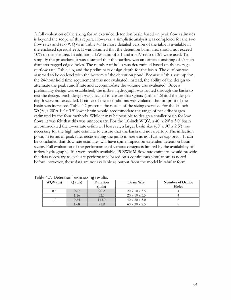
64

A full evaluation of the sizing for an extended detention basin based on peak flow estimates is beyond the scope of this report. However, a simplistic analysis was completed for the two flow rates and two WQVs in Table 4.7 (a more detailed version of the table is available in the enclosed spreadsheet). It was assumed that the detention basin area should not exceed 10% of the site area. In addition a L:W ratio of 2:1 and a H:V ratio of 3:1 were used. To simplify the procedure, it was assumed that the outflow was an orifice consisting of ½-inch diameter ragged edged holes. The number of holes was determined based on the average outflow rate, Table 4.6, and the preliminary design depth for the basin. The outflow was assumed to be on level with the bottom of the detention pond. Because of this assumption, the 24-hour hold time requirement was not evaluated; instead, the ability of the design to attenuate the peak runoff rate and accommodate the volume was evaluated. Once a preliminary design was established, the inflow hydrograph was routed through the basin to test the design. Each design was checked to ensure that Qmax (Table 4.6) and the design depth were not exceeded. If either of these conditions was violated, the footprint of the basin was increased. Table 4.7 presents the results of the sizing exercise. For the ½-inch WQV, a 20’ x 10’ x 3.5’ lower basin would accommodate the range of peak discharges estimated by the four methods. While it may be possible to design a smaller basin for low flows, it was felt that this was unnecessary. For the 1.0-inch WQV, a 40’ x 20’ x 3.0’ basin accommodated the lower rate estimate. However, a larger basin size (60’ x 30’ x 2.5’) was necessary for the high rate estimate to ensure that the basin did not overtop. The inflection point, in terms of peak rate, necessitating the jump in size was not further explored. It can be concluded that flow rate estimates will have some impact on extended detention basin sizing. Full evaluation of the performance of various designs is limited by the availability of inflow hydrographs. If it were readily available, PCSWMM flow rate estimates would provide the data necessary to evaluate performance based on a continuous simulation; as noted before, however, these data are not available as output from the model in tabular form.

Table 4.7: Detention basin sizing results.

WQV (in) Q (cfs) Duration (min)

Basin Size Number of Orifice Holes

0.5 0.67 90.2 20 x 10 x 3.5 4 1.16 52.1 20 x 10 x 3.5 4

1.0 0.84 143.9 40 x 20 x 3.0 6 1.68 71.9 60 x 30 x 2.5 8

65

5. Conclusions The Massachusetts Department of Environmental Protection (Mass DEP) contracted with the University of Massachusetts’ Water Resources Research Center (WRRC) to conduct an evaluation of a PC version of EPA’s Stormwater Management Model (PCSWMM, Version 1.0, Build 5.0.144) to determine whether it accurately converts the Water Quality Volume MassDEP requires for sizing of stormwater treatment practices to an equivalent flow rate. In this project, WRRC also evaluated the adequacy of three additional methods identified as the Ahlfeld, Bryant, and Claytor methods to convert the 1-inch and ½ inch Water Quality Volume required by the Massachusetts Stormwater Standards to an equivalent flow rate. The models were evaluated using default parameters and assumptions to provide information and a recommendation to MassDEP on the relative accuracy of the model to conform to the MassDEP’s required Water Quality Volume based standard. Third party studies that were used to calibrate the PCSWMM Model were also evaluated as to their robustness. Project results are intended to help inform MassDEP about the appropriate use of, and reliance upon, PCSWMM model results. Key findings of the evaluation include: The theoretical basis of the PCSWMM model appears sound based on a review of its

technical construct. It is worth noting that its formulation is analogous to version 4.3 of the EPA SWMM model.

PCSWMM is sensitive to the resolution of the precipitation data utilized for design. It is recommended that only 15-minute data be utilized.

The default PCSWMM parameters are generally reasonable, although alternative values for the following may be preferable: lower Manning’s n values for impervious areas, lower Manning’s n values for pervious areas, lower minimum infiltration rate, and a lower infiltration regeneration rate. However, a sensitivity study found that model results are insensitive to any of these parameters in terms of both volume and rate. Runoff is typically 93 to 95% of the rainfall depth.

PCSWMM flow rate estimates are most sensitive to site size. While the field studies used to corroborate PCSWMM do not contradict the model

results, nor are they generally robust enough to confirm its results. Of the studies, the Como Park, Minnesota study and to a lesser extent the Edmonton, Alberta study provide some degree of validation.

The Ahlfeld, Bryant, and Claytor methods evaluated for conversion of a WQV to a flow rate are based solely on hydrology. These methods result in a large range of flow rate estimates for a given WQV.

The effect of routing and flow-path are not accounted for by any of the models, including PCSWMM.

The effect of precipitation falling as snow rather than rain is not accounted for by any of the models, including PCSWMM.

The Claytor method is the most complete in attempting to define the WQV based on precipitation and site characteristics, as well as transforming the resulting depth to a flow rate. However, the first step of this analysis has not been completed specifically for Massachusetts.

The frequency level most appropriate for design is not evident from either the Bryant or Ahlfeld methods.

66

Current PCSWMM output cannot be used to infer a flow rate for a given WQV. For an equivalent annual runoff cumulative frequency, PCSWMM typically predicts a

lower flow rate than the other methods for the 1-inch WQV (as defined by the alternative methods). These differences tend to decrease for higher cumulative probabilities and return periods. It is important to recall, however, that this cannot be considered a 1:1 comparison.

PCSWMM is distinct among the studied methods in basing unit sizing on TSS loading and removal (which are both driven by the site hydrology).

PCSWMM suggested sizing is equivalent to that which would be selected based on the alternative flow methods 40% of the time for the 1-inch WQV and 64% of the time for the ½-inch WQV. The instances where PCSWMM would undersize in comparison to the alternative methods are associated with higher percentages of the annual precipitation (Bryant), longer return-intervals (Ahlfeld), and larger WQVs (Claytor). A requirement that unit sizing be set such that 80% of the TSS load and that the unit design capacity flow rate be sized to accommodate the rate equivalent to 98% of the annual cumulative runoff would result in an equivalent sizing between methods in all but the most extreme cases.

PCSWMM results are significantly influenced by influent particle size distribution as well as the temporal resolution of rainfall data. Removal efficiencies increase and recommended unit size decreases as coarser PSDs are assumed.

Flow rate estimates will have some impact on extended detention basin sizing, but this will be highly site dependent.

The basis for PCSWMM sizing, and that of similar flow through devices, is the percent sediment removal achieved for a given site based on 15-minute washoff predicted for a given PSD and the associated settling characteristics. PCSWMM does not base sizing decisions on flow rate, although flow rate is an important factor impacting sediment delivery and removal. A key feature of these flow through devices is that they achieve much of their sediment removal at low flows. Traditional methods of stormwater sizing are based on flood prevention with an emphasis on storage volume and peak attenuation. However, for water quality purposes, a large percentage of the annual load is delivered by small, more frequent events as well as the first flush of large events. There is thus a divergence in the basis of design for water quality and flood protection. The comparison of PCSWMM against three alternative sizing methods presented in this report exemplifies the underlying differences of these approaches. Water quality treatment designs based on a WQV assume that it is necessary to capture a high level of the annual flow in order to achieve the desired water quality load reduction. Continuous water quality and flow models such as PCSWMM attempt to directly simulate water quality load reduction. Unfortunately, it is difficult to confirm which design methodology (flow based or load reduction based) is most conservative without robust field studies. Longer-term continuous data sets and models are necessary to fully evaluate the benefits and limitations of water quality treatment design based on peak flow rate or a single event volume versus longer-term load reduction.

67

6.0 References

Adams, B.J. and F. Papa. 2000. Urban Stormwater Management Planning with Analytical

Probabilistic Models, New York: John Wiley & Sons, Inc. Ahlfeld, D.P. and M. Minihane. 2004. Storm flow from first-flush precipitation in stormwater design. Journal of Irrigation and Drainage Engineering, 130:4, pp. 269 – 276. American Society of Civil Engineers. 1992. Design and Construction of Urban Stormwater

Management Systems. New York, New York: American Society of Civil Engineers. Applied Hydrology Associates. 2003. The Effects of Backwater on Stormceptor Treatment Systems Denver Colorado Area.

Associated Earth Sciences, Inc. 2001. SeaTac Stormceptor Performance Monitoring Report. Kirkland Washington. Barbe, D.E., J.F. Cruise, and X. Mo. 1996. Modeling the buildup and washoff of pollutants

on urban watersheds. Water Resources Bulletin, 32(3), 511-519. Bryant, G.. Massachusetts Rainfall Intensity Analysis. Unpublished, undated manuscript submitted to MassDEP. Butler D. and J.W. Davies. 2000. Urban Drainage. London: E & FN Spon. Charbeneau, R.J. and M.E. Barrett. 1998. Evaluation of methods for estimating stormwater

pollutant loads. Water Environment Research, Vol. 70, No. 7, 1295. Chen, J. and B.J. Adams. 2006. Analytical urban storm water quality models based on

pollutant buildup and washoff processes. Journal of Environmental Engineering, Vol. 132, No. 10, 1314.

Chin, D.A.. 2006. Water Resources Engineering, 2nd edition. Upper Saddle River, New Jersey:

Prentice Hall. Chow, V.T. 1959. Open-Channel Hydraulics. McGraw-Hill: New York, New York. Claytor, R.A. and T.R. Schueler. 1996. Design of Stormwater Filtering Systems. Silver Spring, MD:

Center for Watershed Protection. Computational Hydraulics International & Imbrium System, Incorporated, 2007. PCSWMM

for Stormceptor Instruction Manual. Dingman, S.L. 2002. Physical Hydrology, 2nd Edition. Upper Saddle River, New Jersey: Prentice

Hall.

68

Donigian, A.S. and W.C. Huber. 1991. Modeling of Nonpoint Source Water Quality in Urban and Non-urban Areas. EPA/600/3-91/039. Washington, DC: US Environmental Protection Agency.

Driver, N.E., M.H. Mustard, R.B. Rhinesmith, and R.F. Middelburg. 1985. U.S. Geological

Survey Urban-Stormwater Data Base for 22 Metropolitan Areas throughout the United States. Open-File Report 85-357. US Geological Survey: Denver, CO:.

Farnsworth, R.K, E.S. Thompson, and E.L. Peck. 1982. Evaporation Atlas for the Contiguous 48

United States. NOAA Technical Report NWS 33. Office of Hydrology, National Weather Service: Washington, D.C., 26 pp. + Appendices.

Farnsworth, R.K. and E.S. Thompson. 1982. Mean Monthly, Seasonal, and Annual Pan

Evaporation for the United States. NOAA Technical Report NWS 34. Office of Hydrology, National Weather Service: Washington, D.C., 82 pp. + Appendices.

Geiger, W.F. and H.R. Dorsch. 1980. Quantity-Quality Simulation (QQS): A Detailed

Continuous Planning Model for Urban Runoff Control, Volume 1. Model Description, Testing, and Applications. EPA/600/2-80-011. Cincinnati, OH: US Environmental Protection Agency.

Gregory, J.H., M.D. Dukes, P.H. Jones and G.I. Miller. 2006. Effect of urban soil

compaction on infiltration rate. Journal of Soil and Water Conservation, 61(3), 117 – 124. Hicks, W.I. 1944. A method of computing urban runoff. Transactions of the American Society of

Civil Engineers, 109:1217. Horton, R.E. 1939. Analysis of runoff plat experiments with varying infiltration capacity.

Transactions of the American Geophysical Union, 20. Horton, R.E.. 1940. An approach toward a physical interpretation of infiltration-capacity.

Soil Science Society of America Journal, 5, 399 – 417. Huber, W.C., J.P. Heaney, D.A. Aggidis, R.E. Dickinson, K.J. Smolenyak, and R.W. Wallace.

1982. Urban rainfall-runoff-quality data base. EPA/600/S2-81/238. Cincinnati, OH: US Environmental Protection Agency.

Huber, W.C. 1985. Deterministic modeling of urban runoff quality, in H.C. Torno, J.

Marsalek, and M. Desbordes eds., Urban Runoff Pollution, Series G: Ecological Sciences, vol. 10. Springer-Verlag: New York, pp. 167-242.

Huff, F.A., and J.R. Angel. 1992. Rainfall Frequency Atlas of the Midwest. Illinois State Water

Survey, Champaign, IL, Bulletin 71, 141 pp. Hydrologic Engineering Center. 1977. Storage, Treatment, Overflow Runoff Model STORM.

Generalized computer Program 723-58-L7520. Hydrologic Engineering Center, U.S. Corps of Engineers, Davis, California.

69

Imbrium Systems, Incorporated, 2008. Correspondence between Daniel Nason, Imbrium, and Thomas Maguire, MA DEP. April 28, 2008. Subject: PCSWMM for Stormceptor Submission. Kahler, D.M. and W. Brutsaert. 2006. Complementary relationship between daily

evaporation in the environment and pan evaporation. Water Resources Research, Vol. 42, W05413.

Kanso, A., M.C. Gromaire, E. Gaume, B. Tassin, and G. Chebbo. 2003. Bayesian approach

for the calibration of models: application to a urban stormwater pollution model. Water Science and Technology, 47(4), 77-84.

Lee, B., F. Tonto, and P. Tov. Undated. Analysis of long term rainfall to develop stormwater quality

flow rate design criteria. Stormceptor Group of Companies: Toronto, Ontario. Maidment, D.R. (editor). 1992. Handbook of Hydrology. New York: McGraw Hill Inc. Manning, R.. 1889. On the flow of water in open channels and pipes. Transactions of the

Institute of Civil Engineers of Ireland, 20, 161-195. Manning, R.. 1895. On the flow of water in open channels and pipes. Transactions of the

Institute of Civil Engineers of Ireland, Supplement to 1889 paper, 24, 179-207. McCuen, R.H. 1998. Hydrologic Analysis and Design. Prentice Hall. Upper Saddle River,

New Jersey. McKay, M. and D.S. Wilks. 1995. Atlas of Short-duration Precipitation Extremes for the Northeastern

United States and Southeastern Canada. Northeast Regional Climate Center Publication No. RR 95-1. Cornell University: Ithaca, New York.

Massachusetts STrategic Envirotechnology Partnership. 2003. Fact Sheet #4: Stormwater Technology: Stormceptor. University of Massachusetts, Amherst MA. Mustard, M.H., Driver, N.E., Chyr, J. and Hansen, B. (1987) U.S. Geological Survey Urban

Stormwater Data Base of Constituent Storm Loads; Characteristics of Rainfall, Runoff, and Antecedent Conditions; and Basin Characteristics. Water-Resources Investigations Report 87-4036. USGS, Books and Open-File Reports Section, Federal Center, Box 25425, Denver, CO. 80225.

Novotny, V. 2003. Water Quality: Diffuse Pollution and Watershed Management, 2d ed.,

New York: John Wiley & Sons, Inc. Novotny, V. and G. Chesters. 1981. Handbook of Nonpoint Pollution Sources and Management.

Van Nostrand Reinhold Company: New York, New York. NSF International and U.S. EPA. 2000. ETV Verification Protocol for Urban Runoff Models – Draft 2.0, October 2000. http://www.epa.gov/etv/pubs/04_vp_runoff.pdf

70

Obropta, C.C. and J.S. Kardos. 2007. Review of urban stormwater quality models: deterministic, stochastic, and hybrid approaches. Journal of the American Water Resources Association, Vol. 43, No. 6, 1508.

Pecher, R. 1969. The runoff coefficient and its dependence on rain duration. Berichte aus dem

Institut fur Wasserwirtschaft und Gesundheitsingenieurwesen, No. 2. TU Munich. The Phoenix Group. 1996. Urban Runoff Pollution Mitigation Study. Edmonton Alberta. Pitt, R. 1994. Small storm hydrology. University of Alabama - Birmingham. Unpublished

manuscript. Presented at design of stormwater quality management practices. Madison, WI May 17-19, 1994.

Rawls, W.J., P. Yates, and L. Asmussen. 1976. Calibration of selected infiltration equations for the

Georgia Coastal Plain, Technical Report ARS-S-113. Washington, D.C.: U.S. Department of Agriculture, Agricultural Research Service.

Rawls, W.J. 1982. Estimation of soil water properties. Transactions of the American Society of

Agricultural Engineers, 25(5), 1316 – 1320 & 1328. Rinker Materials. 2002. Stormceptor Monitoring Study Como Park St. Paul Minnesota. Robien, A, T. Striebel, and R. Herrmann. 1997. Modeling of dissolved and particle-bound

pollutants in urban street runoff. Water Science and Technology, 36(8-9), 77-82. Sartor, J.D. and G.B. Boyd. 1972. Water Pollution Aspects of Street Surface Contaminants. EPA-

R2-72-081, U.S. Environmental Protection Agency: Washington, D.C. Sartor, J.D., G.B. Boyd, and F.J. Agardy. 1974. Water pollution aspects of street surface

contaminants. Journal – Water Pollution Control Federation, 46(3), 458-467. Schueler, T.R. 1987. Controlling Urban Runoff: A Practical Manual for Planning and Designing Urban

BMPs. Washington D.C.: Metropolitan Washington Council of Governments. Skaggs, R.W. and R. Khaleel. 1982. “Infiltration”, in C.T. Haan, ed., Hydrologic Modeling of

Small Watersheds, Monograph 5, American Society of Agricultural Engineers, St. Joseph, Mich., pp. 4-166, 1982.

Stormceptor Group of Companies. 2004. Field Evaluation of a Stormceptor Model STC 1200 Westwood, MA. Stormwater Assessment Monitoring and Performance Program. 2004.Performance Assessment of Two Types of Oil and Grip Separator for Stormwater Management in Parking Lot Applications – Markham and Toronto, Ontario. Technology Acceptance Reciprocity Partnership. 2003. TARP Tier II protocol,

http://www.mastep.net/documents/TARP%20Tier2protocol.doc.

71

Tholin, A.L. and C.J. Keifer. 1960. The hydrology of urban runoff. Transactions of the American Society of Civil Engineers, 125:1308.

Tsihrintzis, V.A. and R. Hamid. 1998. Runoff quality prediction from small urban

catchments using SWMM. Hydrological Processes, Vol. 12, 311-239. U.S. EPA. 1983. Results of the Nationwide Urban Runoff Program, Volume I – Final Report. NTIS

PB84-185552. U.S. Environmental Protection Agency: Washington, D.C. U.S. Natural Resources Conservation Service (formerly the Soil Conservation Service). 1986.

Urban Hydrology for Small Watersheds, Technical Release 55. United States Department of Agriculture: Washington, D.C.

U.S. Natural Resources Conservation Service. 2002. WinTR-55 User Manual. United States

Department of Agriculture: Washington, D.C. Vaze, J. and F.H.S. Chiew. 2003. Comparative evaluation of urban storm water quality

models. Water Resource Research, Vol. 39, No. 10, 1280. Viessman, W., Jr. 1968. Runoff estimation for very small drainage areas. Water Resources

Research, 4(1), 87-93. Viessman, W., J. Knapp, and G. L. Lewis. 1977. Introduction to Hydrology, 2d ed., New York:

Harper & Row. Water Resources Research Center. 2009. MASTEP data screening tool

http://www.mastep.net/database/docs.cfm#review University of Massachusetts, Amherst MA.

Wilks, D.S. and R. P. Cember. 1993. Atlas of Precipitation Extremes for the Northeastern United

States and Southeastern Canada. Northeast Regional Climate Center Publication No. RR 93-5. Cornell University: Ithaca, New York.

Water Resources Research Center. 2009. PCSWMM Evaluation Quality Assurance Project

Plan. University of Massachusetts, Amherst MA. Winkler, E.S. 1998. Technology Assessment, Stormceptor. University of Massachusetts,

Amherst MA. Winkler, E., D. Ahlfeld, G. Askar, and M. Minihane. 2001. Final Report: Development of a

Rational Basis for Designing Recharging Stormwater Control Structures and Flow and Volume Design Criteria. Center for Energy Efficiency and Renewable Energy, University of Massachusetts Amherst.

72

Appendices Alternate Methods 1. PCSWMM Sensi.xls Comparative Sizing – PCSWMM vs. STEP 2. Hyannis Base Design Table NJDEP 80.doc 3. Hyannis Base Design Table User 80.doc 4. Hyannis Sizing Summary Brief NJDEP 50.doc 5. Hyannis Sizing Summary Brief User 50.doc 6. PCSWMM_STEP_Compare.xls Field Evaluations 7. Como Pk PCSWMM NJDEP PSD.doc 8. Como Pk PCSWMM EPA NURP PSD.doc 9. Como Pk PCSWMM Fine Default PSD.doc 10. PCSWMM Field Evaluations.xls Extended Detention Basin Sizing 11. EDDB Design.xls