PCF extended with real numbers - School of …mhe/papers/realpcf.pdf · 2001-03-07 · PCF extended with real numbers Mart´ın H¨otzel Escard´o ... Of course, the PCF interpreter

PCF extended with real numbers

Martın Hotzel Escardo

Department of Computing, Imperial College, 180 Queen’s Gate,London SW7 2BZ, United Kingdom, E-mail: [email protected]

Abstract

We extend the programming language PCF with a type for (total and partial)real numbers. By a partial real number we mean an element of a cpo of intervals,whose subspace of maximal elements (single-point intervals) is homeomorphic tothe Euclidean real line. We show that partial real numbers can be considered as“continuous words”. Concatenation of continuous words corresponds to refinementof partial information. The usual basic operations cons, head and tail used to ex-plicitly or recursively define functions on words generalize to partial real numbers.We use this fact to give an operational semantics to the above referred extensionof PCF. We prove that the operational semantics is sound and complete with re-spect to the denotational semantics. A program of real number type evaluates toa head-normal form iff its value is different from ⊥; if its value is different from ⊥then it successively evaluates to head-normal forms giving better and better partialresults converging to its value.

Keywords: Exact real number computation. Domain Theory and Interval Analysis.Denotational and operational semantics.

1 Introduction

There are several practical and theoretical approaches to exact real numbercomputation (see eg. [7–9,18,21,24,26,30,31,37,39,40,42]). However, the authoris not aware of any attempt to give denotational and operational semanticsto an implementable programming language with a data type for exact realnumbers. Most approaches to exact real number computation are based onrepresentation of real numbers in other data types, such as streams of digitsor rational numbers. P. di Gianantonio [9] discusses an extension of PCF withstreams and shows how to represent real numbers in this extension (see below).

In this paper we extend the programming language PCF [28] with a typefor real numbers. This type is interpreted as the cpo of intervals introducedindependently by R.M. Moore in the 60’s [25] and by D.S. Scott in the

To appear in Theoretical Computer Science, July 1996

early 70’s [32]. In fact, such an extension was one of the problems left openby G.D Plotkin [28]. It is straight-forward to give a denotational semantics tosuch an extension, but it is not immediate how to give an operational seman-tics to it. P. di Gianantonio also presents an extension of PCF with a groundtype interpreted as an algebraic cpo of real numbers, but he does not give anoperational semantics to it.

An important feature of our approach to exact real number computation isthat the programmer does not have access to representations within the pro-gramming language and can think of real numbers as abstract entities in theusual mathematical sense. Of course, the PCF interpreter has access only toconcrete representations. The correct interaction between the abstract leveland the concrete level is usually referred to as the Adequacy Property (of theoperational semantics with respect to the denotational semantics). At the de-notational level, a PCF program is just a mathematical expression denotinga number or a function. The task of the programmer is to find a mathemat-ical expression denoting the entity that he or she has in mind. This entityis usually given by unrestricted mathematical means. In this case the pro-grammer has to find an equivalent PCF expression. The Adequacy Propertyensures that the entity denoted by the program will actually be computed bythe PCF interpreter, and this is why the programmer is not concerned withrepresentations.

We refer to the elements of the cpo of intervals as “partial real numbers”. Thedomain of partial numbers is a non-algebraic continuous cpo. Its subspace ofmaximal elements (single-point intervals) is homeomorphic to the Euclideanreal line, so that real numbers are special cases of partial real numbers. Noticethat no algebraic cpo can have this property.

We show that partial real numbers can be considered as “continuous words”,in the sense that they can be given the structure of a monoid, in such away that it has a submonoid isomorphic to the monoid of words over anyfinite alphabet. Moreover, as it is the case for words, the prefix preorder ofthe monoid of continuous words coincides with its information order. Thiscoincidence is the basis for the successful interaction between the operationaland denotational semantics of PCF extended with real numbers.

Concatenation of continuous words have intuitive geometrical and compu-tational interpretations. Geometrically, a concatenation of continuous wordscorresponds to a rescaling of an interval followed by a translation (an affinetransformation). Computationally, a concatenation of continuous words corre-sponds to refinement of partial information; in a concatenation xy the partialreal number y refines the information given by x, by selecting a subintervalof x.

2

The notion of length of words generalizes to partial real numbers. The lengthof a partial real number is an extended non-negative real number, being in-finity iff the partial number is maximal, and zero iff the partial number isbottom. Roughly speaking, the length of a partial number x considered as apartial realization of an unknown real number y gives the number of digits ofan expansion of y that x is able to give correctly. The concatenation operation“adds lengths”, in the sense that the length function is a monoid homomor-phism from the monoid of partial real numbers to the additive monoid ofnon-negative extended real numbers.

The usual basic operations cons, head and tail used to explicitly or recursivelydefine functions on words generalize to partial real numbers. Geometrically,the operation cons is an affine transformation (in analytic terms, a linear map)on the unit interval, tail reverses the effect of cons, and head decides in whichhalf of the real line its argument lies, telling us nothing in ambiguous cases.

Concatenation of partial numbers can be infinitely iterated. This fact gives anotion of meaningful infinite computation. The concatenation of finite initialsegments of infinite computations gives more and more information about thefinal result, in such a way that every piece of information about the (ideal)result is eventually produced in a finite amount of steps. In practice, the termsof a computation can be taken as the partial numbers with distinct rationalend-points.

The interpretation of partial real numbers as continuous words is related toa well-known approach to real number computation. Usual binary expansionsare not appropriate representations for real number computation; for instance,multiplication by three is not computable if we read the expansions from left toright [42]. But binary expansions of numbers in the signed unit interval [−1, 1]allowing a digit −1 turn out to be effective [8,9,17,40–42]. In the domain ofpartial numbers contained in the signed unit interval, infinite concatenations ofthe partial numbers [−1, 0], [− 1

2, 1

2] and [0, 1] correspond to binary expansions

of numbers in the signed unit interval using the digits −1, 0 and 1 respectively.

We use the fact that partial real numbers can be considered as continuouswords to obtain an operational semantics for the extension of PCF referredabove. We prove that the operational semantics enjoys the following AdequacyProperty: a program of real number type evaluates to a head-normal form iffits value is different from ⊥; if its value is different from ⊥ then it succes-sively evaluates to head-normal forms giving better and better partial resultsconverging to its value.

To be accurate, the interpretation of partial numbers as continuous wordsholds only for the domain of partial real numbers contained in the unit interval(or any other compact interval). The domain of partial number contained in

3

the unit interval is referred to as the lazy unit interval, and the domain of allpartial real numbers is referred to as the lazy real line. The above results areextended from the lazy unit interval to the lazy real line via an action of thelazy unit interval on the lazy real line.

Organization

In Section 2 we briefly introduce the domain-theoretic and topological aspectsof partial real numbers which are relevant to this paper. In Section 3 we developthe idea that “partial real numbers are continuous words”. In Section 4 weextend PCF with partial real numbers. Finally, in Section 5 we present someconcluding remarks and directions for further work.

2 The domain of partial real numbers

2.1 Domains

Our main references to Domain Theory are [3] and [16]. The widely circulatednotes [29] are an excellent introduction, but they do not cover (non-algebraic)continuous cpos. The book [19] contains all the domain-theoretic materialneeded to understand PCF (without real numbers) as well as a detailed ac-count to PCF. In this paper a (continuous Scott) domain is defined to be abounded complete ω-continuous cpo; notice that a Scott domain is usuallydefined to be a bounded complete ω-algebraic cpo. In Section 3 we make useof elementary domain theory only, and therefore the reader can think of adomain just as a bounded complete cpo. But in Section 4 we make essentialuse of continuity, implicitly in the use of function spaces and explicitly in theproof of the Adequacy Theorem 34.

When we refer to a dcpo as a topological space we mean its set of elementsunder its Scott topology [3,16,35].

2.2 The lazy real line

We denote by R the set of non-empty compact subintervals of the real lineordered by x v y iff x ⊇ y; see Moore [25] and Scott [32]. If we add abottom element to the continuous dcpo R, which can be concretely taken asthe interval (−∞, +∞), then R becomes a domain, referred to as the lazy realline.

4

For the topological connections between Domain Theory and Interval Anal-ysis [25] see [15]. In particular, it is shown that the Scott open sets are theMoore open upper sets. Since Moore restricts himself to monotone functions,the results presented in [25] go through if we replace the Moore topology bythe Scott topology. See also [4] for more connections between Domain Theoryand Interval Analysis.

Following the points of view of both Moore and Scott, we do not considerthe elements of R as intervals. We instead consider them as generalized realnumbers, in a similar way that complex numbers are considered as generalizedreal numbers, and we call them partial real numbers. The maximal partial realnumbers (that is, the singleton intervals) are identified with the real numbers.This identification makes sense from a topological view, because the subspaceof maximal elements of R is homeomorphic to the Euclidean real line. Non-maximal partial real numbers can be considered as partial realizations of realnumbers. For example, [3.14, 3.15] can be considered as a partial realizationof π (and of several other numbers). Hence the designation partial real number.

A subset of the lazy real line has a join iff it has an upper bound; when thejoin exists, it is the intersection of the subset. Every subset of the lazy real linehas a meet, namely the least interval (most defined partial number) containingthe union of the set.

We denote the left and right end-points of a partial number x by x and xrespectively, so that x = [x, x].

Two partial numbers x and y have an upper bound iff they overlap. In thiscase their join is the overlapping part; that is, x t y = [max(x, y), min(x, y)].Dually, we have that their meet is given by x u y = [min(x, y), max(x, y)].

The way-below relation on the lazy real line is given by x ¿ y iff x = ⊥, orx < y and y < x. Therefore, a basis for the lazy real line is given by the setcontaining ⊥ and the non-maximal partial numbers with rational (respectivelydyadic) end-points. Recall that a dyadic number is a rational of the form m/2n.

2.3 Order of magnitude on the lazy real line

We define a strict order < on partial numbers (not to be confused with thestrict version @ of the information order or with the way-below order ¿) byx < y iff x < y. This relation is clearly irreflexive, transitive, and asymmetric,in the sense that x < y together with x > y is impossible.

We say that two elements x and y of a domain are consistent, written x ' y, ifthey have a common upper bound. The consistency relation is always reflexive

5

and symmetric, but not transitive, and it is preserved by monotone maps.

The following proposition is immediate:

Proposition 1 For all partial real numbers x and y, exactly one of the rela-tions x < y, x ' y and x > y holds.

We define a relation ≤ on partial numbers (not to be confused with the in-formation order v) by x ≤ y iff x ≤ y. This relation does not enjoy any ofthe properties that an order relation should satisfy, and therefore the notationcan be misleading. We introduce it only for notational convenience.

2.4 The lazy unit interval

The set I of all partial numbers contained in the unit interval [0, 1] is a domain,referred to as the lazy unit interval. The bottom element of I is the partialnumber [0, 1]. Its way-below order is given by x ¿ y iff x = 0 or x < y, andy < x or y = 1.

The lazy unit interval can be presented in a geometrically more convenientform as follows. The unit square [0, 1]× [0, 1] under the componentwise orderinduced by the usual order ≤ on [0, 1] is a continuous lattice, whose Lawsontopology coincides with the Euclidean topology on the unit square; see [16] fora proof of these facts. If we consider the points below (equivalently, on the leftof) the diagonal which goes from (0, 1) to (1, 0), that is, the points (x, y) withx + y ≤ 1, we get a triangle, which we refer to as the unit triangle. The unittriangle is easily seen to be a domain. Its maximal elements are the points(x, y) with x + y = 1, that is, the points on the diagonal.

It turns out that the unit triangle is isomorphic to the lazy unit interval. Theisomorphisms can be taken as (x, y) 7→ [1 − y, x] and [x, y] 7→ (y, 1 − x). Wecan think of the unit triangle as a coordinate system for the lazy unit interval.

We have a similar fact for the lazy real line; a coordinate system for R is givenby the half-plane consisting of the points (x, y) with x + y ≤ 0. A coordinatesystem for R⊥ is obtained by adding a point (−∞,−∞) to the half-plane.

3 Partial real numbers considered as continuous words

Subsections 3.1–3.7 are restricted to the lazy unit interval and Subsection 3.8extends the results of these sections to the lazy real line.

6

3.1 The prefix preorder of a monoid

Recall that a monoid is a set together with a binary associative operation and aneutral element for this operation. It is customary to refer to this operation asmultiplication, but in this paper it is convenient to refer to it as concatenation.

By a word over an alphabet Σ we mean either a finite word in Σ∗ or an infiniteword in Σω. We denote the set of all words by Σ∞. Usual concatenation ofwords, with the convention that xy = x if x is infinite, makes Σ∞ into amonoid with neutral element the empty word ε.

In any monoid (M, ·, e) we can define a preorder, called its prefix preorder,by x ≤ z iff xy = z for some y. In this case x is called a prefix of z and yis called a suffix. This relation is reflexive because e is right neutral, and itis transitive because the concatenation operation is associative. It has e asits least element because e is left neutral. Monoid homomorphisms preservethe least element and the prefix preorder, by the very definition of monoidhomomorphism. An element x is maximal iff it is left dominant, in the sensethat xy = x for every y. The meet of a set, when it exists, is the greatestcommon prefix of the elements of the set.

The prefix preorder of the monoid Σ∞ makes the set Σ∞ into a Scott do-main [35]. In particular, the prefix preorder is a partial order; that is, it isantisymmetric. An element of Σ∞ is maximal iff it is an infinite word, and itis finite in the domain-theoretic sense iff it is a finite word. The concatenationoperation seen as a function Σ∞ × Σ∞ → Σ∞ is not continuous, because itis not even monotone. But it is continuous on its second argument. This canbe expressed by saying that left translations x 7→ ax are continuous for allwords a.

3.2 Left translations of a monoid

We denote a left translation x 7→ ax of a monoid (M, ·, e) by consa. Lefttranslations are monotone and consa(M) = ↑↑a, where ↑↑a = x ∈ M |a ≤ x.An element a is left cancelable iff the translation consa is injective.

If x is left cancelable and x ≤ z, we denote the unique y such that xy = zby z/x, so that x(z/x) = z. The basic properties of this (partially defined)quotient operation are:

x/e = x

x/x = e

7

(y/x)(z/y) = z/x

(xy)/z = (x/z)y

when the quotients are defined.

Let a be a left cancelable element of a monoid M . Then the co-restrictionof consa to its image is a bijection between the sets M and ↑↑a, with inversex 7→ x/a. Therefore M is a preordered set isomorphic to the set ↑↑a under theinherited order, because consa is monotone.

The left cancelable elements of Σ∞ are the finite words. It follows that ↑↑ais a domain isomorphic to Σ∞ for every finite word a. The subsection belowshows that the lazy unit interval has the same property for every non-maximalpartial number a, for a suitable concatenation operation on partial numbers.

3.3 Concatenation of partial real numbers

Define a binary operation (x, y) 7→ xy on I by

xy = [(x− x)y + x, (x− x)y + x]

That is, given x, y ∈ I, rescale and translate the unit interval so that it be-comes x, and define xy to be the interval which results from applying the samerescaling and translation to y. Then it is immediate that xy is a subintervalof x. The rescaling factor is the diameter of x, namely x − x, and the trans-lation constant is the left end-point of x. If x is maximal, then its diameteris zero, so that xy = x. In order to simplify notation, we let κx stand for thediameter of x and µx stand for the left end-point of x. This is the notationof [23] for affine transformations. Notice that x = [µx, µx + κx]. Then we canwrite

xy = κxy + µx

Theorem 2 (I, ·,⊥) is a monoid with the following properties:

(i) Its prefix preorder coincides with the information order of the domain I.(ii) Its left cancelable elements are the non-maximal ones.(iii) Its left translations preserve all meets and all existing joins.

Proof. Let x, y, z ∈ I. Then

xy = κxy + µx = κx[µy, µy + κy] + µx = [κxµy + µx, κx(µy + κy) + µx]

8

Hence µxy = κxµy + µx and κxy = κxκy. Therefore

(xy)z = κxyz + µxy = κxκyz + κxµy + µx = κx(κyz + µy) + µx = x(yz)

Now, clearly x⊥ = x, because by definition⊥ = [0, 1] is rescaled and translatedso that it becomes x. Also, ⊥x = x because by definition ⊥ = [0, 1] is rescaledand translated so that it becomes itself; hence ⊥x is the application of theidentity to x. Therefore (I, ·,⊥) is a monoid.

(i) By construction, x v xy. If x v z and x is maximal, then xy = x = z forevery y. The proof of item (ii) shows that if x v z and x is non-maximal thenthere is a (unique) y such that xy = z.

(ii) A rescaling is reversible iff the rescaling factor is non-zero, a translation isalways reversible, and an element has diameter zero iff it is maximal.

(iii) The linear maps p 7→ κxp + µx are either increasing order isomorphismsbetween the real line and itself (if κx > 0) or else constant maps (if κx = 0). 2

The above proof shows that the concatenation operation on partial numbers“multiplies diameters”, in the sense that κxy = κxκy. Therefore κxy ≤ κx andκxy ≤ κy, the equalities holding iff x = ⊥ or y = ⊥.

Concatenation of partial numbers has the following geometrical and compu-tational interpretations. In a concatenation xy, the interval y refines the in-formation given by x by selecting a subinterval of x. For example, the partialnumbers [0, 1], [0, 1

2], [ 1

2, 1], and [1

3, 2

3] respectively select the whole interval, the

first half, the second half, and the middle third part. Thus, concatenation ofpartial numbers allows for incremental computation on partial real numbers,also known as lazy evaluation (cf. Proposition 4). Hence the denomination lazyunit interval.

There is yet another geometrical interpretation of concatenation, induced bythe isomorphism between the lazy unit interval and the unit triangle. The up-per set of any non-maximal element x of the unit triangle is clearly a triangle,isomorphic to the unit triangle via a rescaling of the unit triangle followed bya translation. Thus, any element y can be interpreted either as an absoluteaddress of a point in the unit triangle or else as a relative address of a point inthe smaller triangle generated by x, namely the point xy, obtained by applyingthe same rescaling and translation to y.

We finish this subsection with the following lemma:

Lemma 3 The bases of the lazy unit interval consisting of respectively all non-maximal partial numbers and all non-maximal partial numbers with rational

9

end-points are submonoids of (I, ·,⊥) closed under existing quotients, in thesense that if b and c are basis elements with b v c then c/b is a basis elementtoo.

Proof. Existing quotients are given by

y/x = (y − µx)/κx =def [(y − µx)/κx, (y − µx)/κx)]

Therefore, if x and y have distinct (rational) end-points, so does y/x. 2

The basis consisting of all non-maximal partial numbers with dyadic end-points is a submonoid, but it is not closed under existing quotients.

3.4 Infinitely iterated concatenations

Let M be a monoid with a partial prefix order and joins of non-decreasingω-chains, and let 〈xn〉n≥1 be a sequence of elements of M . Then we have that

x1 ≤ x1x2 ≤ · · · ≤ x1x2 · · · xn ≤ · · ·

The infinitely iterated concatenation of 〈xn〉n≥1 is defined to be the join ofthese partial concatenations, informally denoted by x1x2 · · · xn · · ·. It is alsoconvenient to use the informal notation y1 t y2 t · · · t yn t · · · for the join ofa chain y1 ≤ y2 ≤ · · · ≤ yn ≤ · · ·.

An interval expansion of a partial real number x is a sequence of intervals〈xn〉n≥1 such that x = x1x2 · · ·xn · · ·. For example, interval expansions formedfrom the intervals

[0,

1

10

],

[1

10,

2

10

], . . . ,

[8

10,

9

10

],

[9

10, 1

]

are essentially decimal expansions.

If we think of an infinitely iterated concatenation as a computation, the fol-lowing proposition shows that we can compute in an incremental fashion ifleft translations are continuous:

Proposition 4 (Infinite associativity) Let M be a monoid with infinitelyiterated concatenations. Then M satisfies the ω-associativity law

10

x1(x2 · · · xn · · ·) = x1x2 · · ·xn · · ·

iff left translations preserve joins of non-decreasing ω-chains.

Proof. (⇒) Assume that the ω-associativity law holds, let 〈yn〉n≥1 be a non-decreasing ω-chain of elements of M , and let 〈xn〉n≥1 be a sequence of elementsof M such that ynxn = yn+1. Then the join of the chain is the same as theinfinitely iterated concatenation of the sequence 〈xn〉n≥1 with y1 added as anew first element, because y1x1x2 · · · xn = yn, as an inductive argument shows.Therefore

a(y1 t y2 t · · · t yn t · · ·) = a(y1x1x2 · · · xn · · ·)= ay1x1x2 · · · xn · · ·= a t ay1 t ay1x1 t · · · t ay1x1 · · · xn t · · ·= a t ay1 t ay2 t · · · t ayn t · · ·= ay1 t ay2 t · · · t ayn t · · ·

(⇐) Assume that left translations preserve joins of non-decreasing ω-chains.Then we have that

x1(x2 · · · xn · · ·) = x1(x2 t x2x3 t · · · t x2x3 · · ·xn t · · ·)= x1x2 t x1x2x3 t · · · t x1x2x3 · · · xn t · · ·= x1 t x1x2 t x1x2x3 t · · · t x1x2x3 · · · xn t · · ·= x1x2 · · ·xn · · · 2

We denote the infinitely iterated concatenation xx · · · x · · · of a constant se-quence with range x by xω. An immediate consequence of the above proposi-tion is that xω is the least fixed point of consx for any monoid with infiniteconcatenations.

Now let y1 ≤ y2 ≤ · · · ≤ yn ≤ · · · be a chain of left cancelable elements. Thenthe sequence y1, y2/y1, y3/y2, . . . , yn+1/yn, . . . has the elements of the chainas partial concatenations. Therefore the join of the chain is the same as theinfinite concatenation of the induced sequence.

Proposition 5 Consider the bases of I consisting of respectively all non-maximal partial numbers and all non-maximal partial numbers with rationalend-points. Then there is a bijection between ω-chains of basis elements andsequences of basis elements, taking any chain to a sequence whose infinitelyinterated concatenation is the join of the chain. 2

11

Therefore we can replace ω-chains of basis elements by (arbitrary) sequencesof basis elements and work with infinitely iterated concatenations instead ofjoins.

For monoids with infinitely interated concatenations, it is natural to ask ho-momorphisms to preserve them.

Proposition 6 A monoid homomorphism preserves infinitely iterated con-catenations iff it preserves joins of increasing ω-chains

Proof. Let h : L → M be a monoid homomorphism between monoids Land M .

(⇒) Let 〈yn〉n≥1 be an non-decreasing ω-chain of elements of L having a joinand let 〈xn〉n≥1 be a sequence of elements of L such that ynxn = yn+1. Thenwe have that

h(y1 t · · · t yn t · · ·)= h(y1x1 · · · xn · · ·)= h(y1)h(x1) · · ·h(xn) · · ·= h(y1) t h(y1)h(x1) t · · · t h(y1)h(x1) · · ·h(xn) t · · ·= h(y1) t · · · t h(yn) t · · ·

because h(yn)h(xn) = h(yn+1).

(⇐) Let 〈xi〉i≥1 be a sequence of elements of L having an infinitely iteratedconcatenation. Then we have that

h (x1x2 · · · xn · · ·) = h (x1 t x1x2 t · · · t x1x2 · · · xn t · · ·)= h(x1) t h(x1x2) t · · · t h(x1x2 · · · xn) t · · ·= h(x1) t h(x1)h(x2) t · · · t h(x1)h(x2) · · ·h(xn) t · · ·= h(x1)h(x2) · · ·h(xn) · · · 2

3.5 Continuous words

Concatenation of partial numbers in the lazy unit interval generalizes concate-nation of words over any finite alphabet, in the following sense:

Proposition 7 For every finite n-letter alphabet Σ, the monoid Σ∞ is iso-morphic to a submonoid of I. Moreover, the induced embedding of Σ∞ into Iis a continuous monoid homomorphism.

12

Proof. Without essential loss of generality, we prove the claim for the two-letter case Σ = 0, 2. Let C be the submonoid of I finitely generated by thepartial numbers [0, 1/3] and [2/3, 1]. Then C clearly contains the partial num-bers corresponding to the intervals successively produced in the constructionof the Cantor set. Hence the joins of strictly increasing ω-chains of elementsof C are the elements of the Cantor set. But these joins are the infinitelyiterated concatenations of the generators. The set C of finite and infinite con-catenations of the generators is also a submonoid of I, which can be consideredas the monoid of partial Cantor numbers. It is easy to see that 0, 2∞ is iso-morphic to C. We know that 0, 2∗ is the free monoid over 0, 2. Hence thereis a unique monoid homomorphism h : 0, 2∗ → C such that h(0) = [0, 1/3]and h(2) = [2/3, 1]. But h has a unique continuous extension to 0, 2∞, be-cause monoid homomorphisms are monotone and 0, 2∗ consists of the finiteelements (in the domain-theoretic sense) of 0, 2∞. The resulting extensionis a monoid homomorphism. Since it takes an infinite word x to the elementof the Cantor set whose ternary expansion is x, it follows that h is a bijection,and therefore a monoid isomorphism. 2

Therefore, the elements of the lazy unit interval can be considered as “continu-ous words”. For any word x ∈ Σ∞ let length(x) ∈ [0,∞] denote the length of xdefined in the usual way. For any continuous word x ∈ I and any real numberb > 1 we define lengthb(x) ∈ [0,∞] to be − logb(κx). Thus, lengthb(x) = ∞iff x is maximal, and lengthb(x) = 0 iff x is bottom.

If a continuous word x is a partial realization of an unknown real number y,then lengthb(x) is the number of correct digits of an expansion to base b of ythat x allows us to know. For example, if we consider x = [0.143, 0.145] as apartial realization of an unknown real number y then length10(x) is roughly 2.7,meaning that x allows us to know two decimal digits of y.

Proposition 8 Consider [0,∞] as a monoid under addition and as a domainunder its prefix preorder (which coincides with its natural order).

(i) For every real number b > 1, lengthb : I → [0,∞] is a continuous monoidhomomorphism.

(ii) Let h be the embedding of the monoid of words over a finite n-letteralphabet into I defined in Proposition 7. Then length = lengthn+1 h.

Proof. Routine verification. The first part follows from the fact that the con-catenation operation multiplies diameters and that logarithms take multipli-cation to addition. 2

Corollary 9 The infinitely iterated concatenation of a sequence of continuouswords is maximal iff the sum of the lengths of the continuous words is ∞.

13

Proof. The length function is a continuous monoid homomorphism and apartial number has infinite length iff it is maximal. 2

The following proposition allows us to prove some properties of real numberprograms. We say that a map f : I → I is guarded if there is a real numberδ > 0 such that length(f(x)) ≥ length(x) + δ, called a guarding constantfor f . Clearly, left translations consa with a 6= ⊥ are guarded, with guardingconstant length(a).

Proposition 10 Any continuous guarded map f : I → I has a maximalpartial number as its unique fixed point.

Proof. Since length(fn(⊥)) ≥ nδ for every n and length is a continuoushomomorphism, length (

⊔n fn(⊥)) ≥ supn nδ = ∞. This means that the least

fixed point of f is maximal. Therefore it is the unique fixed point of f . 2

3.6 Heads and tails of continuous words

We begin by considering the head and tail maps on words over the alphabetΣ = 0, 1.

Let σ range over Σ, and define maps tail : Σ∞ → Σ∞ and head : Σ∞ → Σ⊥

tail(ε) = ε

tail(σx) = x

head(ε) =⊥head(σx) = σ

These maps are continuous, and we have that

tail(consσ(x)) = x

head(consσ(x)) = σ

Recall that a pair of continuous maps s : D → E and r : E → D betweendcpos D and E with the property that

r s = id

14

is called a section-retraction pair [3]. In this case s preserves all existing meetsand joins, and s r is an idempotent.

By definition, tail is a retraction and consσ is a section. Recall also that if inaddition the induced idempotent has

s rv id

then the pair of maps s and r are said to be an embedding-projection pair. Thepair of maps tail and consσ are not an embedding-projection pair, because forexample

cons0(tail(ε)) = 0 6v ε = id(ε)

Now define a continuous equality map (x, y) 7→ (x =⊥ y) : Σ⊥×Σ⊥ → tt, ff⊥by

(x =⊥ y) =

tt if x, y ∈ Σ and x = y

⊥ if ⊥ ∈ x, yff if x, y ∈ Σ and x 6= y

and a continuous conditional map

(p, x, y) 7→ (if p then x else y) : tt, ff⊥ × Σ∞ × Σ∞ → Σ∞

by

if p then x else y =

x if p = tt

ε if p = ⊥y if p = ff

Then we have that

x = if head(x) =⊥ 0 then cons0(tail(x)) else cons1(tail(x)) (1)

Manipulations of this equation lead to usual explicit and recursive definitionsof several functions. For example, it follows from (1) that the identity functionsatisfies the equation

15

id(x) = if head(x) =⊥ 0 then cons0(id(tail(x))) else cons1(id(tail(x)))

In fact, the identity function is the unique continuous map which satisfies thefunctional equation

f(x) = if head(x) =⊥ 0 then cons0(f(tail(x))) else cons1(f(tail(x)))

The function that switches the roles of the letters 0 and 1 can be given by thethe recursive definition

g(x) = if head(x) =⊥ 0 then cons1(g(tail(x))) else cons0(g(tail(x)))

In this subsection we look for a generalization of this theme for partial num-bers. The first problem to be overcome is that continuous words have non-integral lengths and in particular non-zero lengths < 1. Moreover, a continu-ous word of length > 1 has infinitely many prefixes of length 1. Since the headmap on words extracts a prefix of length 1, it is not immediately clear whatthe head map on continuous words should be for words of length < 1.

Under the embedding of Σ∞ into I defined in Proposition 7, if we put

l = [0, 1/3] and r = [2/3, 1]

then Equation (1) becomes

x = if x <⊥ 12

then consl(x/l) else consr(x/r) (1′)

where the conditional map is defined in the same way for partial numbersand the continuous comparison map (x, y) 7→ (x <⊥ y) : I × I → tt, ff⊥ isdefined by

(x <⊥ y) =

tt if x < y

⊥ if x ' y

ff if x > y

Remark 11 If we had x <⊥ x = ff then this map would not be continu-ous. 2

Then we need a continuous map taila : I → I, for any left cancelable partialnumber a, with the property that

taila(x) = x/a for every x with x v a,

16

that is, with the property that taila is a left-inverse of consa. A naıve attemptto obtain such a map would be to put taila(x) = ⊥ if x 6v a. But then tailawould not be continuous.

Lemma 12 Let a ∈ I be a non-maximal element, let taila : I → I be anycontinuous left inverse of consa, and let fa be the induced idempotent. Thenfor every x ∈ I,

(i) a v fa(x)(ii) fa(x) = x iff a v x(iii) taila(x) = fa(x)/a

Proof. (1) a v consa(taila(x)) = fa(x).

(2) (⇒) Immediate consequence of (1) above. (⇐) If a v x then x = a(x/a)and fa(x) = consa(taila(a(x/a))) = consa(x/a) = x.

(3) taila(x) = consa(taila(x))/a = fa(x)/a. 2

Thus, in order to obtain a continuous left inverse of consa we first look for acontinuous map fa enjoying properties (1) and (2) above. Assume that x ' a.Then fa(x) v fa(x t a) = x t a, because x v x t a. Since a v x t a, by (1)and (2) it is natural to let fa(x) be x t a. Then fa(x) can be thought as thetruncation of x to a, because x t a is the greatest subinterval of x containedin a.

Lemma 13 Let a be an element of I. If joina : I → I is a monotone mapsuch that

joina(x) = x t a for all x ' a.

then joina(x) = a for all x < a and joina(x) = a for all x > a.

Proof. Here we write a to mean [a, a], of course. Assume that x < a. Thismeans that x < a. Then [x, a] v x. Hence a = joina([x, a]) v joina(x). There-fore a = joina(x), because a is maximal. The other case is similar. 2

Lemma 14 For all non-maximal a ∈ I define maps joina, taila : I → I by

17

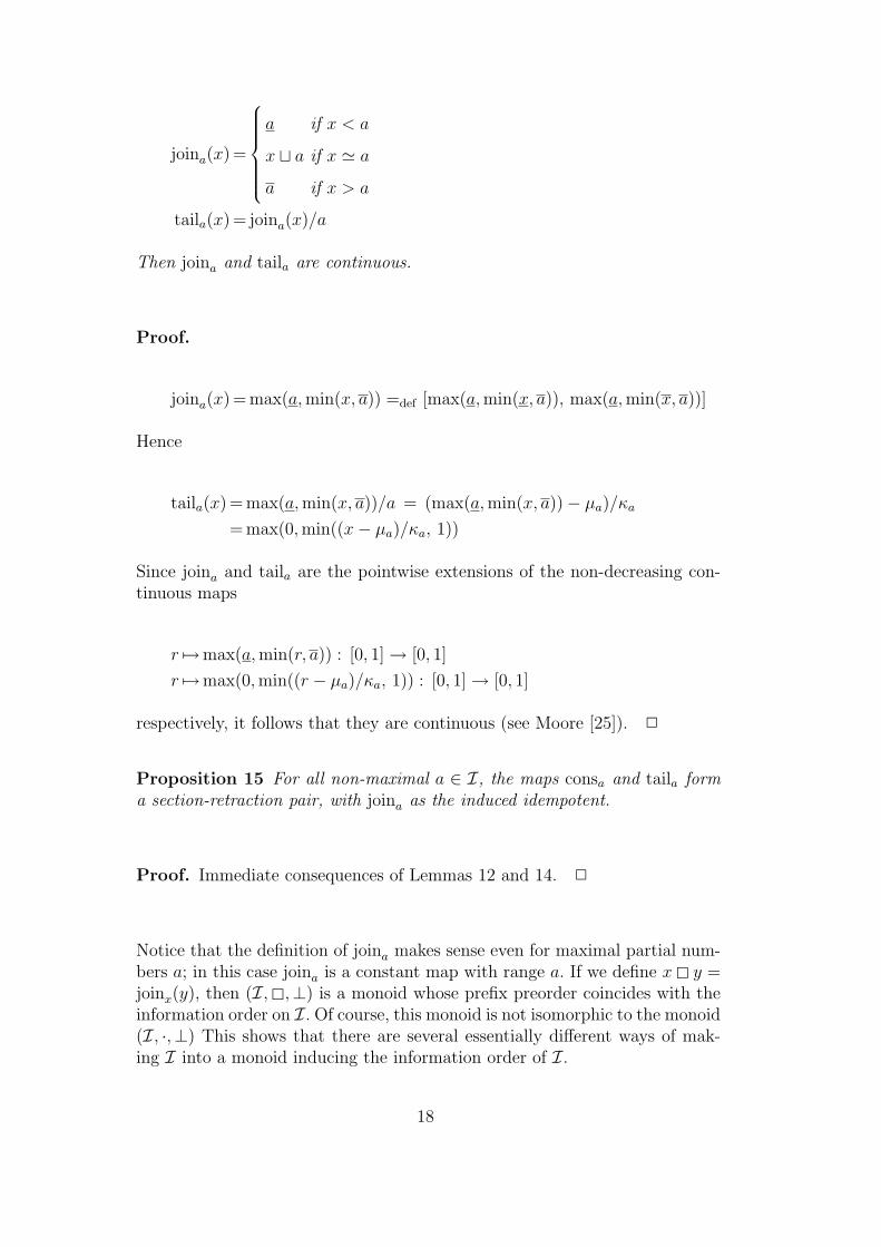
joina(x) =

a if x < a

x t a if x ' a

a if x > a

taila(x) = joina(x)/a

Then joina and taila are continuous.

Proof.

joina(x) = max(a, min(x, a)) =def [max(a, min(x, a)), max(a, min(x, a))]

Hence

taila(x) = max(a, min(x, a))/a = (max(a, min(x, a))− µa)/κa

= max(0, min((x− µa)/κa, 1))

Since joina and taila are the pointwise extensions of the non-decreasing con-tinuous maps

r 7→max(a, min(r, a)) : [0, 1] → [0, 1]

r 7→max(0, min((r − µa)/κa, 1)) : [0, 1] → [0, 1]

respectively, it follows that they are continuous (see Moore [25]). 2

Proposition 15 For all non-maximal a ∈ I, the maps consa and taila forma section-retraction pair, with joina as the induced idempotent.

Proof. Immediate consequences of Lemmas 12 and 14. 2

Notice that the definition of joina makes sense even for maximal partial num-bers a; in this case joina is a constant map with range a. If we define x y =joinx(y), then (I,,⊥) is a monoid whose prefix preorder coincides with theinformation order on I. Of course, this monoid is not isomorphic to the monoid(I, ·,⊥) This shows that there are several essentially different ways of mak-ing I into a monoid inducing the information order of I.

18

The second problem to be overcome is that Equation (1′) is true only for arestricted set of partial numbers x. This problem is partially solved by replac-ing l and r by

L = [0, 12] and R = [ 1

2, 1]

respectively. By replacing the (sequential) conditional by the parallel one,namely (p, x, y) 7→ (pif p then x else y) : tt, ff⊥ × I × I → I defined by

pif p then x else y =

x if p = tt

x u y if p = ⊥y if p = ff

(cf. [28] and Subsection 4.5), the problem is completely solved. Recall that themeet x u y is the greatest common prefix of the continuous words x and y.

Finally, for each r ∈ [0, 1] define headr : I → tt, ff⊥ by

headr(x) = (x <⊥ r)

Theorem 16 For any partial number x ∈ I,

x = pif head 12(x) then consL(tailL(x)) else consR(tailR(x)) (1′′)

Proof. By virtue of Proposition 15, it suffices to check the crucial case x ' 12.

Equation (1′′) is true in this case because

joinL(x) = [x, 12] joinR(x) = [ 1

2, x]

and therefore joinL(x) u joinR(x) = x. 2

Of course, there is nothing special about the number 12and the partial numbers

[0, 12] and [ 1

2, 1]; the above theorem works for any binary partition of the unit

interval, and can be extended to any finite n-ary partition with n ≥ 2.

The idea behind the above theorem is strongly related to the ideas presentedin [14]; see Examples 18, 19, and 25. See also Smyth’s constructions of theunit interval as inverse limits of finite topological structures [36].

Example 17 (Path composition) The parallel conditional can be used toovercome the fact that x <⊥ x is ⊥ instead of ff.

19

Let E be any domain, and let f, g : I → E be continuous maps. Then f and gare (generalized) paths in the domain E. (The restrictions of f and g to thesingleton intervals are paths in the usual sense [20].) If f(1) = g(0) the pathsare said to be composable. Now define a continuous map h : I → E by

h(x) = pif x <⊥ 12

then f(2x) else g(2x− 1)

If the paths are composable, then h is a (generalized) composite path. Let uscheck the crucial case x = 1

2:

h( 12) = pif 1

2<⊥ 1

2then f(2 1

2) else g(2 1

2− 1) = pif ⊥ then f(1) else g(0)

= f(1) u g(0) = f(1) = g(0)

Notice that the sequential conditional would produce ⊥ instead of f(1) u g(0),and therefore h would be undefined at 1

2.

If f and g are not composable, then h is a generalized composite path with ajump at 1

2, namely f(1)ug(0). For instance, if E = I and f and g are constant

maps with range 0 and 1, then h can be thought as a switch which turns on attime 1

2. In this case, the switch is in the transition state [0, 1] = 0u1 at time 1

2.

Notice that even in this case h is Scott continuous, because it is a compositionof continuous maps. 2

The following recursive definitions generalize the recursive definition for realnumbers presented in [14] to partial real numbers.

Example 18 (Complement) We now derive a recursive definition of theextension of the complement map r 7→ 1− r on [0, 1] to I given by

1− x = [1− x, 1− x]

Of course, for maximal partial numbers, this indeed coincides with the originalmap, up to the identification of real numbers and maximal partial numbers.

We begin with the following observation:

(i) If x ⊆ L then 1− x ⊆ R.(ii) If x ⊆ R then 1− x ⊆ L.

This leads one to write down the following set of incomplete equations:

1− consL(x) = 1− consR(· · ·)1− consR(x) = 1− consL(· · ·)

20

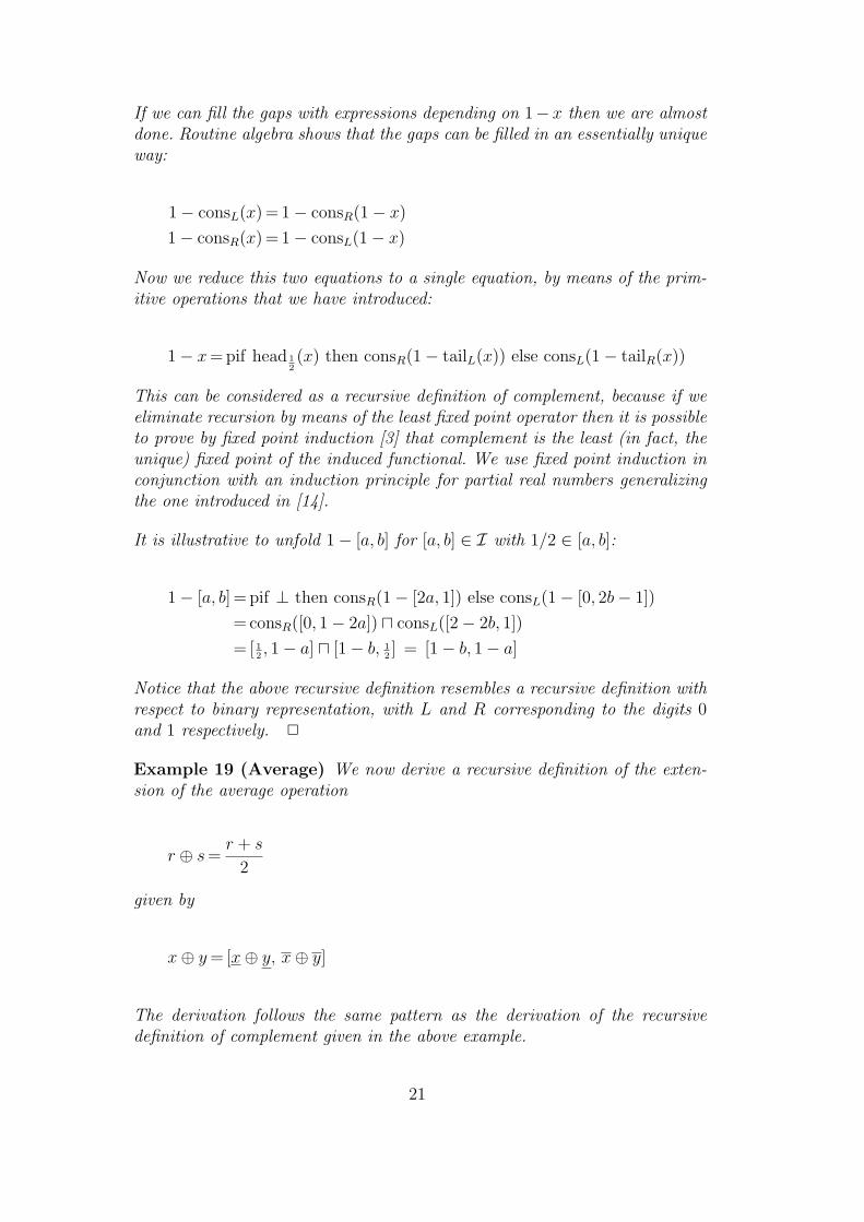
If we can fill the gaps with expressions depending on 1− x then we are almostdone. Routine algebra shows that the gaps can be filled in an essentially uniqueway:

1− consL(x) = 1− consR(1− x)

1− consR(x) = 1− consL(1− x)

Now we reduce this two equations to a single equation, by means of the prim-itive operations that we have introduced:

1− x = pif head 12(x) then consR(1− tailL(x)) else consL(1− tailR(x))

This can be considered as a recursive definition of complement, because if weeliminate recursion by means of the least fixed point operator then it is possibleto prove by fixed point induction [3] that complement is the least (in fact, theunique) fixed point of the induced functional. We use fixed point induction inconjunction with an induction principle for partial real numbers generalizingthe one introduced in [14].

It is illustrative to unfold 1− [a, b] for [a, b] ∈ I with 1/2 ∈ [a, b]:

1− [a, b] = pif ⊥ then consR(1− [2a, 1]) else consL(1− [0, 2b− 1])

= consR([0, 1− 2a]) u consL([2− 2b, 1])

= [ 12, 1− a] u [1− b, 1

2] = [1− b, 1− a]

Notice that the above recursive definition resembles a recursive definition withrespect to binary representation, with L and R corresponding to the digits 0and 1 respectively. 2

Example 19 (Average) We now derive a recursive definition of the exten-sion of the average operation

r ⊕ s =r + s

2

given by

x⊕ y = [x⊕ y, x⊕ y]

The derivation follows the same pattern as the derivation of the recursivedefinition of complement given in the above example.

21

Initial observation:

(i) If x, y ⊆ L then x + y ⊆ L.(ii) If x ⊆ L and y ⊆ R then x + y ⊆ C.(iii) If x, y ⊆ R then x + y ⊆ R.

where C = [1/4, 3/4].

Incomplete equations:

consL(x)⊕ consL(y) = consL(· · ·)consL(x)⊕ consR(y) = consC(· · ·)consR(x)⊕ consL(y) = consC(· · ·)consR(x)⊕ consR(y) = consR(· · ·)

Gaps filled:

consL(x)⊕ consL(y) = consL(x⊕ y)

consL(x)⊕ consR(y) = consC(x⊕ y)

consR(x)⊕ consL(y) = consC(x⊕ y)

consR(x)⊕ consR(y) = consR(x⊕ y)

Reduction to a single equation:

x⊕ y = pif head 12(x) then pif head 1

2(y) then consL(tailL(x)⊕ tailL(y))

else consC(tailL(x)⊕ tailR(y))else pif head 1

2(y) then consC(tailR(x)⊕ tailL(y))

else consR(tailR(x)⊕ tailR(y)),

In practice it may be convenient to use the more familiar notations

x < 12, x/2, x/2 + 1/4, x/2 + 1

2, min(2x, 1), and max(0, 2x− 1)

instead of

head 12(x), consL(x), consC(x), consR(x), tailL(x), and tailR(x)

respectively, and even write 2x and 2x− 1 for the last two cases by an abuseof notation. With this notation the above recursive definition becomes

x⊕ y = pif x < 12

then pif y < 12

then (2x⊕ 2y)/2else (2x⊕ (2y − 1))/2 + 1/4

else pif y < 12

then ((2x− 1)⊕ 2y)/2 + 1/4

22

else ((2x− 1)⊕ (2y − 1))/2 + 12

2

Example 20 (Multiplication) We now derive a recursive definition of mul-tiplication, which is extended in the same way as average. During this examplejuxtaposition means multiplication instead of concatenation. Again, the deriva-tion follows the same pattern.

Initial observation:

(i) If x, y ⊆ L then xy ⊆ [0, 1/4].(ii) If x ⊆ L and y ⊆ R then xy ⊆ [0, 1/2].(iii) If x, y ⊆ R then xy ⊆ [1/4, 1].

Incomplete equations:

consL(x)× consL(y) = cons[0, 1/4](· · ·)consL(x)× consR(y) = cons[0, 1/2](· · ·)consR(x)× consL(y) = cons[0, 1/2](· · ·)consR(x)× consR(y) = cons[1/4, 1](· · ·)

Gaps filled with expressions depending on x, y and xy:

consL(x)× consL(y) = cons[0, 1/4](xy)

consL(x)× consR(y) = cons[0, 1/2]

(x + xy

2

)

consR(x)× consL(y) = cons[0, 1/2]

(xy + y

2

)

consR(x)× consR(y) = cons[1/4, 1]

(x + xy + y

3

)

Now we have to find a recursive definition of ternary average. In this casethere are eight cases to consider, but since the operation is permutative (per-mutativity is the generalization of commutativity to n-ary operations), thereare really only four cases to consider. We omit the routine derivation and thereduction to a single equation. 2

3.7 Computation rules for continuous words

The following lemma shows how to reduce expressions e denoting non-bottompartial numbers to expressions of the form consa(e

′) with a 6= ⊥. Such anexpression is called a head-normal form. The idea is that if an expression ehas a head-normal form consa(e

′) then we know that its value is contained in a.

23

Thus, a head-normal form is a partially evaluated expression. A better partialevaluation of e is obtained by partially evaluating e′, obtaining a head-normalform consb(e

′′), and applying rule (i) below to consa(consb(e′′)) in order to

obtain the more informative head-normal form consab(e′′) of e, and so on.

Lemma 21 For all non-maximal a, b ∈ I and all x ∈ I,

(i) consa(consb(x)) = consab(x)(ii) taila(consb(x)) = Lω if b ≤ a(iii) taila(consb(x)) = Rω if b ≥ a(iv) taila(consb(x)) = consb/a(x) if a v b(v) taila(consb(x)) = cons(atb)/a(tail(atb)/b(x)) if a ' b(vi) headr(consa(x)) = tt if a < r(vii) headr(consa(x)) = ff if a > r(viii) pif tt then x else y = x(ix) pif ff then x else y = y(x) pif p then consa(x) else consb(y) =

consaub(pif p then consa/(aub)(x)else consb/(aub)(y))

Proof. (i) This is the associativity law expressed in terms of left translations.(ii) If b ≤ a then taila(bx) = 0 = [0, 1

2]ω. (iii) Similar.

(iv) Equivalent to the fact that (bx)/a = (b/a)x.

(v) For all c ' x, consb(joinc(x)) = consb(c t x) = consb(c) t consb(x) =joinbc(consb(x)), because left-translations preserve existing joins. Hence

taila(consb(x)) = joina(consb(x))/a = joinatb(consb(x))/a

= joinb((atb)/b)(consb(x))/a = consb(join(atb)/b(x))/a

= consb(cons(atb)/b(tail(atb)/b(x)))/a

= consatb(tail(atb)/b(x))/a = cons(atb)/a(tail(atb)/b(x))

The second step follows from the fact that joina(y) = joinatb(y) if a ' b andb v y. The last step follows from the fact that (cy)/a = (c/a)y.

(vi–ix) Immediate. (x) It suffices to show that

consa(x) u consb(y) = consaub(consa/(aub)(x) u consb/(aub)(y))

Since left translations preserve meets and a = c(a/c) for all c, the result followsby taking c = a u b. 2

24

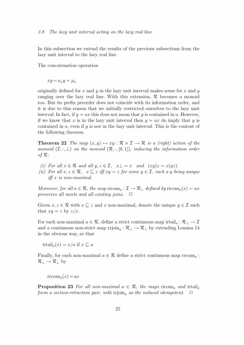
3.8 The lazy unit interval acting on the lazy real line

In this subsection we extend the results of the previous subsections from thelazy unit interval to the lazy real line.

The concatenation operation

xy = κxy + µx

originally defined for x and y in the lazy unit interval makes sense for x and yranging over the lazy real line. With this extension, R becomes a monoidtoo. But its prefix preorder does not coincide with its information order, andit is due to this reason that we initially restricted ourselves to the lazy unitinterval. In fact, if y = ax this does not mean that y is contained in a. However,if we know that x is in the lazy unit interval then y = ax do imply that y iscontained in a, even if y is not in the lazy unit interval. This is the content ofthe following theorem.

Theorem 22 The map (x, y) 7→ xy : R × I → R is a (right) action of themonoid (I, ·,⊥) on the monoid (R, ·, [0, 1]), inducing the information orderof R:

(i) For all x ∈ R and all y, z ∈ I, x⊥ = x and (xy)z = x(yz).(ii) For all x, z ∈ R, x v z iff xy = z for some y ∈ I, such a y being unique

iff x is non-maximal.

Moreover, for all a ∈ R, the map riconsa : I → R⊥ defined by riconsa(x) = axpreserves all meets and all existing joins. 2

Given x, z ∈ R with x v z and x non-maximal, denote the unique y ∈ I suchthat xy = z by z/x.

For each non-maximal a ∈ R, define a strict continuous map irtaila : R⊥ → Iand a continuous non-strict map rrjoina : R⊥ → R⊥ by extending Lemma 14in the obvious way, so that

irtaila(x) = x/a if x v a

Finally, for each non-maximal a ∈ R define a strict continuous map rrconsa :R⊥ →R⊥ by

rrconsa(x) = ax

Proposition 23 For all non-maximal a ∈ R, the maps riconsa and irtailaform a section-retraction pair, with rrjoina as the induced idempotent. 2

25

Thus, I is a retract of R⊥, in many ways. In particular,

(i) ricons[0,1] : I → R⊥ is the inclusion,(ii) irtail[0,1] : R⊥ → I is a “truncated projection”, and(iii) rrjoin[0,1] : R⊥ →R⊥ is the co-extension of the truncated projection.

Example 24 (Addition) We obtain a recursive definition of addition in R⊥by reducing addition to the average operation on I defined in Example 19. Firstnotice that

x + y = pif x < 0 ∨ y < 0 then 2(

x+12

+ y+12

)− 2

else pif x > 1 ∨ y > 1 then 2(

x2

+ y2

)

else 2(

x+y2

)

where ∨ is “parallel or” [28]. Hence

x + y = pif x < 0 ∨ y < 0 then 2(

x+12

+ y+12

)− 2

else pif x > 1 ∨ y > 1 then 2(

x2

+ y2

)

else 2 out(in(x)⊕ in(y))

where in = irtail[0,1] : R⊥ → I and out = ricons[0,1] : I → R⊥.

The operation out is of fundamental importance in this recursive definition; itis this operation that makes the above recursive definition “get off the ground”.More formally, this is a non-strict operation, and some non-strict operationis needed if the fixed point operator (used to solve the above equation) is toproduce a non-bottom solution. If we want to avoid using intermediate mapson the unit interval in recursive definitions of maps on the real line, we can usethe non-strict operation rrjoin to get off the ground. See example below. 2

Multiplication on R⊥ can be obtained in a similar way from multiplicationon I.

Example 25 (Logarithm) The following recursive definition of the loga-rithm function logb, with b > 1, is based on [14]. We first reduce the cal-culation of logb(x) for x arbitrary to a calculation of logb(x) for x ⊆ [1, b],so that logb(x) ⊆ [0, 1], and then recursively consider the cases x =

√x′ and

x =√

bx′′. Notice that such x′ and x′′ are again contained in [1, b], and thatboth cases hold iff x =

√b iff x2 = b. Also, the reduction process diverges if x

contains non-positive numbers.

logb(x) = pif x > b then logb(x/b) + 1else pif x < 1 then logb(bx)− 1

else rrjoin[0,1]

(pif x2 < b then logb(x

2)2

else logb(x2/b)+12

)

26

Recall that rrjoin[0,1](x) = max(0, min(x, 1)). The application of the map rrjointherefore seems redundant, because the tests preceding the recursive call of thelogarithm function in the argument of rrjoin would ensure that the result iscontained in [0, 1]. But the logarithm function is what the recursive definition isdefining and therefore it has to ensure that this is indeed the case. As explainedin Example 24, such a map is needed to “get off the ground”. 2

The head-normal forms for R⊥ are taken as the expressions of the formriconsa(e).

Lemma 26 For all non-maximal a ∈ R and b ∈ I, and all x ∈ I,

(i) (a) rrconsa(rrconsb(x)) = rrconsab(x)(b) rrconsa(riconsb(x)) = riconsab(x)(c) riconsa(consb(x)) = riconsab(x)

(ii) irtaila(riconsb(x)) = Lω if b ≤ a(iii) irtaila(riconsb(x)) = Rω if b ≥ a(iv) irtaila(riconsb(x)) = consb/a(x) if a v b(v) irtaila(riconsb(x)) = cons(atb)/a(tail(atb)/b(x)) if a ' b(vi) rheadr(riconsa(x)) = tt if a < r(vii) rheadr(riconsa(x)) = ff if a > r(viii) pif tt then x else y = x(ix) pif ff then x else y = y(x) pif p then riconsa(x) else riconsb(y) =

riconsaub(pif p then riconsa/(aub)(x)else riconsb/(aub)(y)

where the parallel conditional, the comparison map, and the head map for R⊥are defined in the same way as for I. Notice that the above lemma is Lemma 21with “r” and “i” inserted in appropriate places.

4 PCF extended with real numbers

We introduce two successive extensions of PCF, first with a type for the lazyunit interval (Subsection 4.2) and then with a further type for the lazy realline (Subsection 4.3). We also discuss the issues of canonical evaluation and ofdeterministic evaluation of PCF programs containing parallel features (Sub-sections 4.4 and 4.5 respectively).

For the reader’s convenience we introduce the basic notions of PCF needed inthis paper (Subsection 4.1). See [19] for an excellent textbook account to PCF.

27

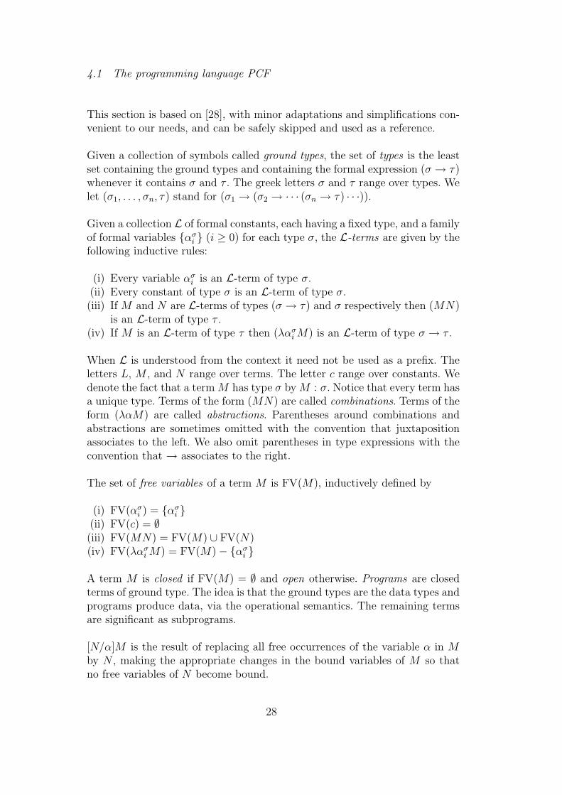
4.1 The programming language PCF

This section is based on [28], with minor adaptations and simplifications con-venient to our needs, and can be safely skipped and used as a reference.

Given a collection of symbols called ground types, the set of types is the leastset containing the ground types and containing the formal expression (σ → τ)whenever it contains σ and τ . The greek letters σ and τ range over types. Welet (σ1, . . . , σn, τ) stand for (σ1 → (σ2 → · · · (σn → τ) · · ·)).

Given a collection L of formal constants, each having a fixed type, and a familyof formal variables ασ

i (i ≥ 0) for each type σ, the L-terms are given by thefollowing inductive rules:

(i) Every variable ασi is an L-term of type σ.

(ii) Every constant of type σ is an L-term of type σ.(iii) If M and N are L-terms of types (σ → τ) and σ respectively then (MN)

is an L-term of type τ .(iv) If M is an L-term of type τ then (λασ

i M) is an L-term of type σ → τ .

When L is understood from the context it need not be used as a prefix. Theletters L, M , and N range over terms. The letter c range over constants. Wedenote the fact that a term M has type σ by M : σ. Notice that every term hasa unique type. Terms of the form (MN) are called combinations. Terms of theform (λαM) are called abstractions. Parentheses around combinations andabstractions are sometimes omitted with the convention that juxtapositionassociates to the left. We also omit parentheses in type expressions with theconvention that → associates to the right.

The set of free variables of a term M is FV(M), inductively defined by

(i) FV(ασi ) = ασ

i (ii) FV(c) = ∅(iii) FV(MN) = FV(M) ∪ FV(N)(iv) FV(λασ

i M) = FV(M)− ασi

A term M is closed if FV(M) = ∅ and open otherwise. Programs are closedterms of ground type. The idea is that the ground types are the data types andprograms produce data, via the operational semantics. The remaining termsare significant as subprograms.

[N/α]M is the result of replacing all free occurrences of the variable α in Mby N , making the appropriate changes in the bound variables of M so thatno free variables of N become bound.

28

4.1.1 The languages LDA, LPA and LPA+∃

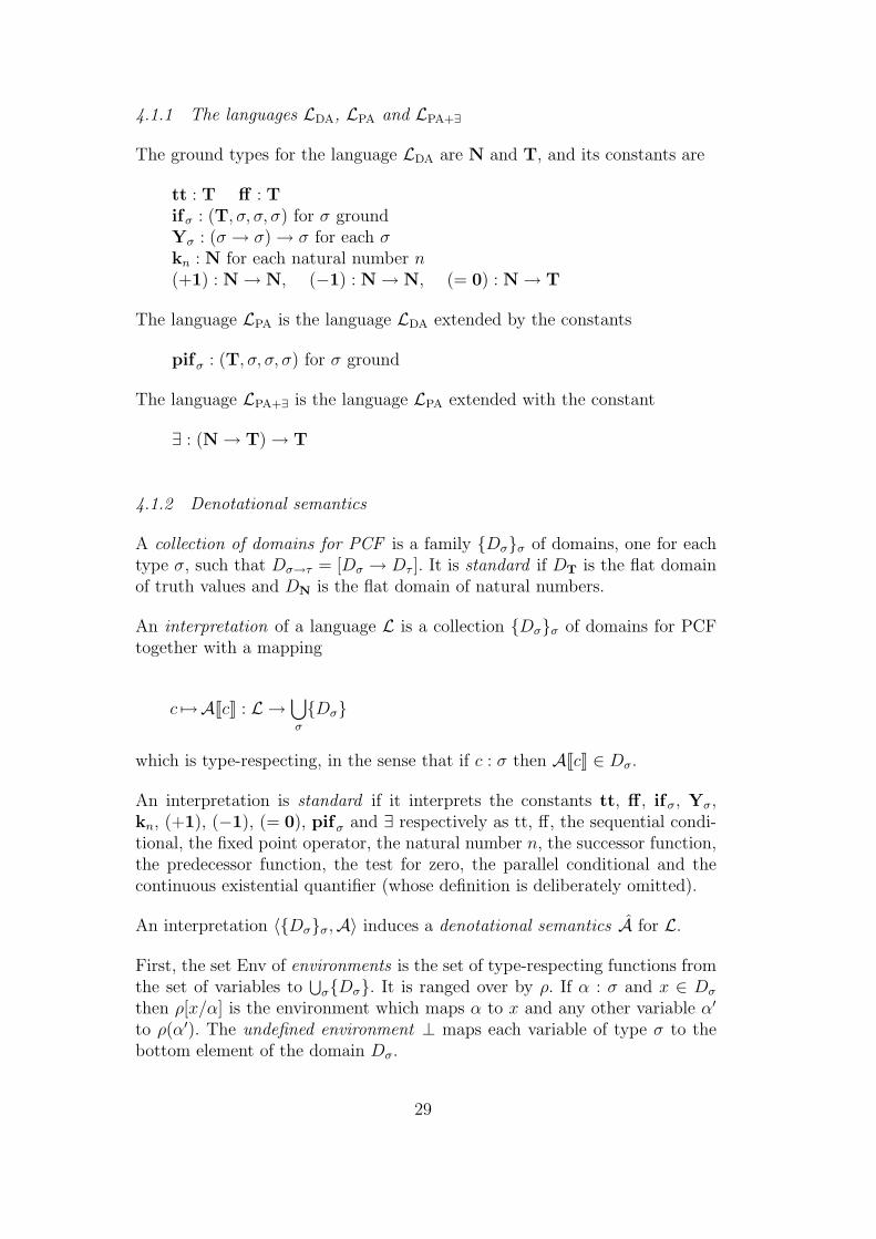
The ground types for the language LDA are N and T, and its constants are

tt : T ff : Tifσ : (T, σ, σ, σ) for σ groundYσ : (σ → σ) → σ for each σkn : N for each natural number n(+1) : N → N, (−1) : N → N, (= 0) : N → T

The language LPA is the language LDA extended by the constants

pifσ : (T, σ, σ, σ) for σ ground

The language LPA+∃ is the language LPA extended with the constant

∃ : (N → T) → T

4.1.2 Denotational semantics

A collection of domains for PCF is a family Dσσ of domains, one for eachtype σ, such that Dσ→τ = [Dσ → Dτ ]. It is standard if DT is the flat domainof truth values and DN is the flat domain of natural numbers.

An interpretation of a language L is a collection Dσσ of domains for PCFtogether with a mapping

c 7→AJcK : L → ⋃σ

Dσ

which is type-respecting, in the sense that if c : σ then AJcK ∈ Dσ.

An interpretation is standard if it interprets the constants tt, ff , ifσ, Yσ,kn, (+1), (−1), (= 0), pifσ and ∃ respectively as tt, ff, the sequential condi-tional, the fixed point operator, the natural number n, the successor function,the predecessor function, the test for zero, the parallel conditional and thecontinuous existential quantifier (whose definition is deliberately omitted).

An interpretation 〈Dσσ,A〉 induces a denotational semantics A for L.

First, the set Env of environments is the set of type-respecting functions fromthe set of variables to

⋃σDσ. It is ranged over by ρ. If α : σ and x ∈ Dσ

then ρ[x/α] is the environment which maps α to x and any other variable α′

to ρ(α′). The undefined environment ⊥ maps each variable of type σ to thebottom element of the domain Dσ.

29

The denotational semantics

M 7→(ρ 7→ AJMK(ρ)

): Terms → (Env → ⋃

σ

Dσ)

is inductively defined by:

(i) AJαK(ρ) = ρ(α)(ii) AJcK(ρ) = AJcK(iii) AJMNK(ρ) = AJMK(ρ)

(AJNK(ρ)

)

(iv) AJλαMK(ρ)(x) = AJMK(ρ[x/α]) (with x ∈ Dσ if α : σ)

Informally,

(i) A variable denotes what the environment assigns to it.(ii) A constant denotes what the interpretation assigns to it.(iii) If a term M denotes the function f : D → E and a term N denotes the

value x ∈ D then the combination MN denotes the value f(x) ∈ E.(iv) If a term M denotes the value yx ∈ E in an environment which assigns

the value x ∈ D to the variable α, then the abstraction λαM denotes thefunction f : D → E defined by f(x) = yx.

If M is closed then its denotation does not depend on the environment, in thesense that AJMK(ρ) = AJMK(ρ′) for all ρ and ρ′.

In order to simplify notation, we let JMK stand for the denotation AJMK(⊥)of a closed term M with respect to an implicit semantics A. Also, for anyterm M , we let JMK(ρ) stand for AJMK(ρ).

4.1.3 Operational semantics

The operational semantics of LDA is given by an immediate reduction relation,defined by the following rules:

(i) (λαM)N → [N/α]M(ii) YM → M(YM)(iii) (+1)kn → kn+1, (−1)kn+1 → kn

(iv) (= 0)k0 → tt, (= 0)kn+1 → ff(v) if ttMN → M , if ffMN → N

(vi) M → M ′MN → M ′N , N → N ′

MN → MN ′ if M is if , (+1), (−1) or (= 0)

We omit the reduction rules of the languages LPA and LPA+∃. The reductionrelation preserves types, in the sense that if M → M ′ and M has type σ, sodoes M ′.

30

Evaluation is given by a partial function Eval from programs to constants,defined by

Eval(M) = c iff M →∗ c

It is well-defined because if M →∗ c and M →∗ c′ then c = c′.

The following theorem is often referred to as the Adequacy Property of PCF.It asserts that the operational and denotational semantics coincide.

Theorem 27 (Plotkin [28], Theorem 3.1) For any LDA program M andconstant c,

Eval(M) = c iff JMK = JcK.

Proof. Lemma 29 below. 2

The following definitions are introduced to formulate and prove Lemma 29.

The predicates Compσ are defined by induction on types by:

(i) If M : σ is a program then M has property Compσ iff JMK = JcK impliesEval(M) = c.

(ii) If M : σ → τ is a closed term it has property Compσ→τ iff wheneverN : σ is a closed term with property Compσ then MN is a term withproperty Compτ .

(iii) If M : σ is an open term with free variables α1 : σ1, . . . , αn : σn then ithas property Compσ iff [N1/α1] · · · [N2/αn]M has property Compσ when-ever N1, . . . , Nn are closed terms having properties Compσ1

, . . ., Compσn

respectively.

A term of type σ is computable if it has property Compσ.

If M : σ → τ and N : σ are closed computable terms, so is MN and also aterm M : (σ1, . . . , σn, τ) is computable iff MN1 . . . Nn is computable wheneverthe terms N1 : σ1, . . . , Nn : σn are closed computable terms and M is a closedinstantiation of M by computable terms.

In the following definitions α has to be chosen as some variable of appropriatetype in each instance. Define terms Ωσ by Ωσ = Yσ(λαα) for σ ground andΩσ→τ = λαΩτ , and define terms Y(n)

σ by Y(0)σ = Ωσ and Y(n+1)

σ = λα(Y(n)σ α).

Then JYσK =⊔

nJYnσK for any standard interpretation.

31

Now define the syntactic information order 4 as the least relation betweenterms such that

(i) Ωσ 4 M : σ and Y(n)σ 4 Yσ,

(ii) M 4 M , and(iii) if M 4 M ′ : σ → τ and N 4 N ′ : σ then λαN 4 λαN ′ and also

MN 4 M ′N ′.

Lemma 28 (Plotkin [28], Lemma 3.2) If M 4 N and M → M ′ theneither M ′ 4 N or else for some N ′, N → N ′ and M ′ 4 N ′.

Proof. By structural induction on M and cases according to why the imme-diate reduction M → M ′ takes place. 2

We include the proof of the following lemma since we are going to extend itto PCF with real numbers:

Lemma 29 (Plotkin [28], Lemma 3.3) Every LDA-term is computable.

Proof. By structural induction on the formation rules of terms:

(1) Every variable is computable since any closed instantiation of it by acomputable term is computable.

(2) Every constant other than the Yσ’s is computable. This is clear for con-stants of ground type. Out of +1, −1, = 0, and if we only consider −1 as anexample. It is enough to show (−1)M computable when M is a closed com-putable term of type N. Suppose J(−1)MK = JcK. Then c = km for some mand so JMK = m + 1. Therefore as M is computable, M →∗ km+1 and so(−1)M →∗ km = c.

(3) If M : σ → τ and N : σ are computable, so is the combination MN . IfMN is closed so are M and N and its computability follows from clause ii ofthe definition of computability. If it is open, any closed instantiation L of it bycomputable terms has the form MN where M and N are closed instantiationsof M and N respectively and therefore themselves computable which in turnimplies the computability of L and hence of MN .

(4) If M : τ is computable, so is the abstraction λαM . It is enough to showthat the ground term LN1 · · ·Nn is computable when N1, · · · , Nn are closedcomputable terms and L is a closed instantiation of λαM by computableterms. Here L must have the form λαM where M is an instantiation of allfree variables of M , except α, by closed computable terms. If JLN1 · · ·NnK =

32

JcK, then we have J[N1/α]MN2 · · ·NnK = JLN1 · · ·NnK = JcK. But [N1/α]Mis computable and so too therefore is MN2 · · ·Nn. Therefore LN1 · · ·Nn →[N1/α]MN2 · · ·Nn →∗ c, as required.

(5) Each Yσ is computable. It is enough to prove YσN1 · · ·Nk is computablewhen N1, · · · , Nk are closed computable terms and YσN1 · · ·Nk is ground.Suppose JYN1 · · ·NkK = JcK. Since JYσK =

⊔nJYn

σK, JY(n)N1 · · ·NkK = JcKfor some n. Since JΩσK = ⊥ for σ ground, Ωσ is computable for σ ground.From this and (1), (3), and (4) proved above it follows that every Ωσ andY(n)

σ is computable. Therefore Y(n)N1 · · ·Nk →∗ c and so by Lemma 28,YN1 · · ·Nk →∗ c, concluding the proof. 2

This lemma extends to the languages LPA and LPA+∃. It suffices to show thatpif and ∃ are computable, with respect to appropriate reduction rules.

4.2 The programming language PCFI

We let L range over the languages LDA, LPA and LPA+∃, and LI denote theextension of L with a new ground type I and the following new constants:

(i) consa : I → I(ii) taila : I → I(iii) headr : I → T(iv) pif I : (T, I, I, I)

for each non-bottom a ∈ I with distinct rational end-points and each rationalr ∈ (0, 1). We refer to the ground type I as the real number type, and toprograms of real number type as real programs.

4.2.1 Denotational semantics

We let DI = I and we extend the standard interpretation A of L to LI by

(i) AJconsaK = consa

(ii) AJtailaK = taila(iii) AJheadrK = headr

(iv) AJpif IKpxy = pif p then x else y

33

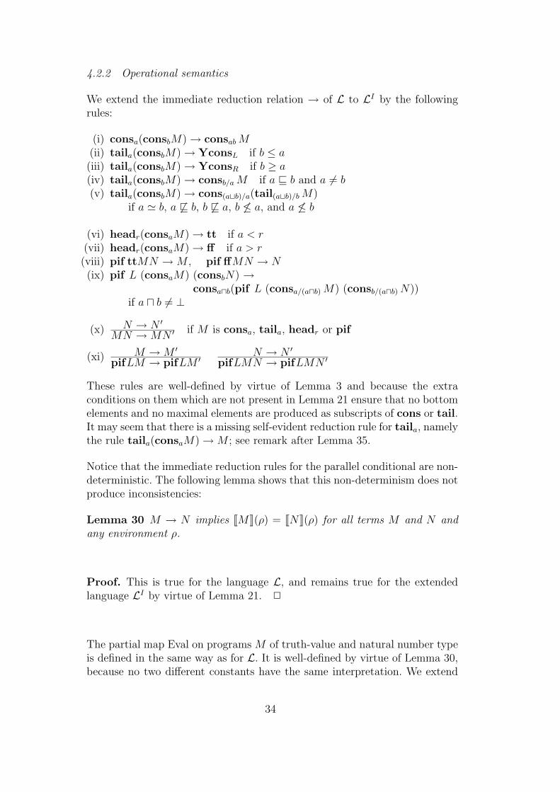
4.2.2 Operational semantics

We extend the immediate reduction relation → of L to LI by the followingrules:

(i) consa(consbM) → consab M(ii) taila(consbM) → YconsL if b ≤ a(iii) taila(consbM) → YconsR if b ≥ a(iv) taila(consbM) → consb/a M if a v b and a 6= b(v) taila(consbM) → cons(atb)/a(tail(atb)/b M)

if a ' b, a 6v b, b 6v a, b 6≤ a, and a 6≤ b

(vi) headr(consaM) → tt if a < r(vii) headr(consaM) → ff if a > r(viii) pif ttMN → M , pif ffMN → N(ix) pif L (consaM) (consbN) →

consaub(pif L (consa/(aub) M) (consb/(aub) N))if a u b 6= ⊥

(x) N → N ′MN → MN ′ if M is consa, taila, headr or pif

(xi) M → M ′pifLM → pifLM ′ N → N ′

pifLMN → pifLMN ′

These rules are well-defined by virtue of Lemma 3 and because the extraconditions on them which are not present in Lemma 21 ensure that no bottomelements and no maximal elements are produced as subscripts of cons or tail.It may seem that there is a missing self-evident reduction rule for taila, namelythe rule taila(consaM) → M ; see remark after Lemma 35.

Notice that the immediate reduction rules for the parallel conditional are non-deterministic. The following lemma shows that this non-determinism does notproduce inconsistencies:

Lemma 30 M → N implies JMK(ρ) = JNK(ρ) for all terms M and N andany environment ρ.

Proof. This is true for the language L, and remains true for the extendedlanguage LI by virtue of Lemma 21. 2

The partial map Eval on programs M of truth-value and natural number typeis defined in the same way as for L. It is well-defined by virtue of Lemma 30,because no two different constants have the same interpretation. We extend

34

Eval to a multi-valued map on real programs M by

Eval(M) = a ∈ I|M →∗ consaM′ for some M ′;

that is, a ∈ Eval(M) iff M has a head-normal form consaM′.

4.2.3 Soundness of the operational semantics

Lemma 31 For all real programs M , a ∈ Eval(M) implies a v JMK.

Proof. By Lemma 30, if M →∗ consaM′ then JMK = JconsaM

′K = aJM ′K.Therefore a v JMK, because the information order on partial numbers coin-cides with the prefix preorder. 2

Theorem 32 (Soundness) For any real program M ,

⊔Eval(M) v JMK

Proof. The join exists because JMK is an upper bound of the set Eval(M).Therefore the result follows from Lemma 31. 2

4.2.4 Completeness of the operational semantics

By virtue of Lemma 31, for any real program M we have that Eval(M) is emptyif JMK = ⊥. The following theorem states a stronger form of the converse:

Theorem 33 (Completeness) For any real program M ,

⊔Eval(M) w JMK

Proof. Lemma 35 below. 2

The soundness and completeness properties in the senses of Theorems 32and 33 can be referred together as the Adequacy Property.

Theorem 34 PCF extended with real numbers enjoys the Adequacy Property.

The recursive definitions given in Examples 18, 19, 20, 24, and 25 give riseto PCF programs in the obvious way. It would be a formidable task to syn-tactically prove the correctness of the resulting programs by appealing to theoperational semantics given by the reduction rules. However, a mathematical

35

proof of the correctness of a recursive definition allows us to conclude that theinduced programs indeed produce correct results, via an application of theAdequacy Theorem. In fact, this is the point of denotational semantics.

We extend the inductive definition of the predicates Compσ by the followingclause:

A real program M has property CompI if for every non-bottom partialnumber x ¿ JMK (as close to JMK as we please) there is some a ∈ Eval(M)with x v a.

If we read the relation x ¿ y as “x is a piece of information about y” thenthe above definition says that a real program is computable if every piece ofinformation about its value can be produced in a finite number of reductionsteps.

The domain-theoretic justificative for continuity of computable functions isthat it is a finiteness condition [29,32,34,35]; a function f is continuous if afinite amount of information about f(x) depends only on a finite amount ofinformation about x. The continuity of a domain, which amounts to its way-below relation being well-behaved, gives us a general and abstract frameworkfor consistently talking about “pieces of information”. Then it should come asno surprise that Lemma 35 makes essential use of the way-below relation andof the continuity of the primitive functions.

The following lemma, which extends Lemma 29, establishes the CompletenessTheorem:

Lemma 35 Every term is computable.

Proof. It suffices to extend the inductive proof of Lemma 29. We have to:

(i) slightly modify the proof for the case of abstractions, because it mentionsconstants and we have added new constants;

(ii) extend the proof of computability of the terms Yσ to the new types; and(iii) show that the new constants are computable.

(i) If M is computable so is λαM :

It is enough to show that the ground term LN1 · · ·Nn is computable whenN1, · · · , Nn are closed computable terms and L is a closed instantiation of λαMby computable terms. Here L must have the form λαM where M is an in-stantiation of all free variables of M , except α, by closed computable terms.Since [N1/α]M is computable, so is [N1/α]MN2 · · ·Nn. Since LN1 · · ·Nn →[N1/α]MN2 · · ·Nn and the reduction relation preserves meaning, in order to

36

evaluate LN1 · · ·Nn it suffices to evaluate [N1/α]MN2 · · ·Nn.

(ii) Yσ is computable for all new types:

In order to prove that Yσ is computable for all new types it suffices to showthat the term Y(σ1,...,σk,I)N1 · · ·Nk is computable whenever N1 : σ1, . . . , Nk : σk

are closed computable terms.

It follows from (i) above that the terms Y(n)σ are computable for all new types,

because the proof of computability of Y(n)σ for old types depends only on the

fact that variables are computable and that the combination and abstractionformation rules preserve computability.

The syntactic information order 4 on L extends to LI , and Lemma 28 is easilyseen to remain true by a routine extension of its inductive proof.

Let x ¿ JYN1 · · ·NkK be a non-bottom partial number. By a basic propertyof the way-below relation of any continuous dcpo, there is some n such thatx ¿ JY(n)N1 · · ·NkK, because JYK =

⊔nJY(n)K. Since Y(n) is computable,

there is a c ∈ Eval(Y(n)N1 · · ·Nk) with x v c. Since there is a term M withY(n)N1 · · ·Nk →∗ conscM and Y(n) 4 Y, it follows from Lemma 28 thatYN1 · · ·Nk →∗ conscM for some M and therefore c ∈ Eval(YN1 · · ·Nk).

(iii) The new constants are computable:

In order to prove that one of the new constants c is computable it suffices toshow that if M1, . . . , Mn are closed computable terms such that cM1 . . .Mn

has real number type, then cM1 . . .Mn is computable.

(iii)(a) consa is computable:

Let M be a computable real program and let x ¿ JconsaMK = aJMK bea non-bottom partial number. We have to produce c ∈ Eval(consaM) withx v c. Let b ¿ JMK with x ¿ ab. If b = ⊥ then we can take c = a.Otherwise let b′ ∈ Eval(M) with b v b′. Then we can take c = ab′, becauseconsaM →∗ consa(consb′M

′) → consab′M′ for some M ′.

(iii)(b) taila is computable:

Let M be a computable real program and let y ¿ JtailaMK = taila(JMK) be anon-bottom partial number. We have to produce c ∈ Eval(tailaM) with y v c.Since taila is continuous, there is some x ¿ JMK such that y ¿ taila(x). Letb ∈ Eval(M) with x v b. It follows that b 6v a, because y 6= ⊥ and if b v athen y ¿ taila(x) v taila(b) v taila(a) = ⊥. Then exactly one of the followingfour cases holds:

(t1) b ≤ a

37

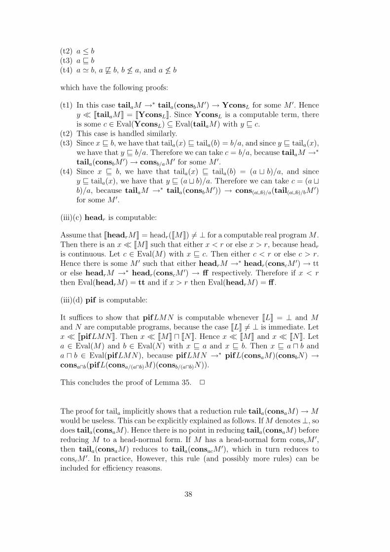
(t2) a ≤ b(t3) a v b(t4) a ' b, a 6v b, b 6≤ a, and a 6≤ b

which have the following proofs:

(t1) In this case tailaM →∗ taila(consbM′) → YconsL for some M ′. Hence

y ¿ JtailaMK = JYconsLK. Since YconsL is a computable term, thereis some c ∈ Eval(YconsL) ⊆ Eval(tailaM) with y v c.

(t2) This case is handled similarly.(t3) Since x v b, we have that taila(x) v taila(b) = b/a, and since y v taila(x),

we have that y v b/a. Therefore we can take c = b/a, because tailaM →∗

taila(consbM′) → consb/aM

′ for some M ′.(t4) Since x v b, we have that taila(x) v taila(b) = (a t b)/a, and since

y v taila(x), we have that y v (a t b)/a. Therefore we can take c = (a tb)/a, because tailaM →∗ taila(consbM

′)) → cons(atb)/a(tail(atb)/bM′)

for some M ′.

(iii)(c) headr is computable:

Assume that JheadrMK = headr(JMK) 6= ⊥ for a computable real program M .Then there is an x ¿ JMK such that either x < r or else x > r, because headr

is continuous. Let c ∈ Eval(M) with x v c. Then either c < r or else c > r.Hence there is some M ′ such that either headrM →∗ headr(conscM

′) → ttor else headrM →∗ headr(conscM

′) → ff respectively. Therefore if x < rthen Eval(headrM) = tt and if x > r then Eval(headrM) = ff .

(iii)(d) pif is computable:

It suffices to show that pifLMN is computable whenever JLK = ⊥ and Mand N are computable programs, because the case JLK 6= ⊥ is immediate. Letx ¿ JpifLMNK. Then x ¿ JMK u JNK. Hence x ¿ JMK and x ¿ JNK. Leta ∈ Eval(M) and b ∈ Eval(N) with x v a and x v b. Then x v a u b anda u b ∈ Eval(pifLMN), because pifLMN →∗ pifL(consaM)(consbN) →consaub(pifL(consa/(aub)M)(consb/(aub)N)).

This concludes the proof of Lemma 35. 2

The proof for taila implicitly shows that a reduction rule taila(consaM) → Mwould be useless. This can be explicitly explained as follows. If M denotes⊥, sodoes taila(consaM). Hence there is no point in reducing taila(consaM) beforereducing M to a head-normal form. If M has a head-normal form conscM

′,then taila(consaM) reduces to taila(consacM

′), which in turn reduces toconscM

′. In practice, However, this rule (and possibly more rules) can beincluded for efficiency reasons.

38

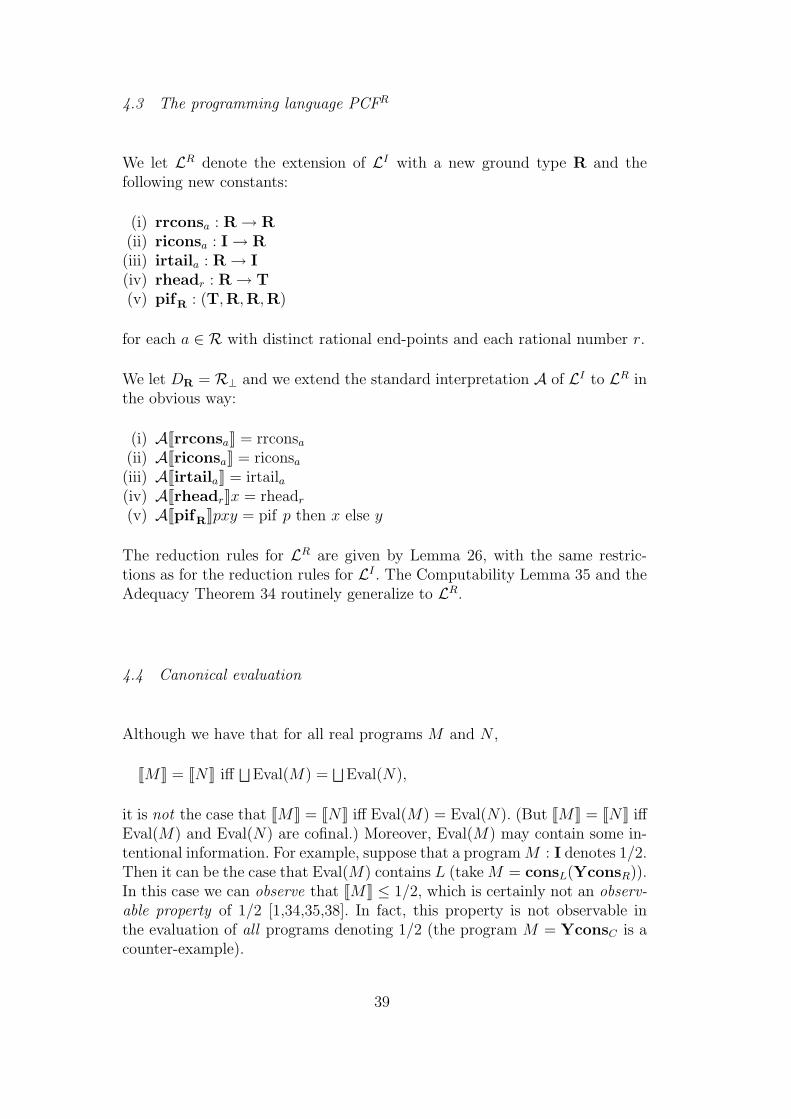
4.3 The programming language PCFR

We let LR denote the extension of LI with a new ground type R and thefollowing new constants:

(i) rrconsa : R → R(ii) riconsa : I → R(iii) irtaila : R → I(iv) rheadr : R → T(v) pifR : (T,R,R,R)

for each a ∈ R with distinct rational end-points and each rational number r.

We let DR = R⊥ and we extend the standard interpretation A of LI to LR inthe obvious way:

(i) AJrrconsaK = rrconsa

(ii) AJriconsaK = riconsa

(iii) AJirtailaK = irtaila(iv) AJrheadrKx = rheadr

(v) AJpifRKpxy = pif p then x else y

The reduction rules for LR are given by Lemma 26, with the same restric-tions as for the reduction rules for LI . The Computability Lemma 35 and theAdequacy Theorem 34 routinely generalize to LR.

4.4 Canonical evaluation

Although we have that for all real programs M and N ,

JMK = JNK iff⊔

Eval(M) =⊔

Eval(N),

it is not the case that JMK = JNK iff Eval(M) = Eval(N). (But JMK = JNK iffEval(M) and Eval(N) are cofinal.) Moreover, Eval(M) may contain some in-tentional information. For example, suppose that a program M : I denotes 1/2.Then it can be the case that Eval(M) contains L (take M = consL(YconsR)).In this case we can observe that JMK ≤ 1/2, which is certainly not an observ-able property of 1/2 [1,34,35,38]. In fact, this property is not observable inthe evaluation of all programs denoting 1/2 (the program M = YconsC is acounter-example).

39

Both problems can be solved by hiding the intensional information containedin Eval(M) as follows. Add an immediate reduction rule

consaM → consb(consa/bM) if b v a and b 6= a,

and define a strong head-normal form to be a real program of the formconsa(consbM) with 0 < b < 1. It follows that a real program M has astrong head-normal form consa(consbM

′) iff a ¿ JMK, because a ¿ x iffthere is some b such that 0 < b < 1 and ab v x. Now, for all real programs M ,define

Eval′(M) = a ∈ I|M has a strong head-normal form consa(consbM′).

With this definition it is immediate that⊔

Eval′(M) =⊔

Eval(M) and

JMK = JNK iff Eval′(M) = Eval′(N),

because

Eval′(M) = a ∈ I|a ¿ JMK and a has distinct rational end-points.

It is also possible to show that, for any standard enumeration of the rationalnumbers, the set Eval′(M) is recursively enumerable. Recall that an enumera-tion r0, r1, . . . , rn, . . . of the rational numbers is standard if there are recursivemaps s, p, q : N→ N such that

rn = (−1)s(n) p(n)

q(n),

and recall that the basic operations and predicates on rational numbers arerecursive with respect to any standard enumeration. In order to prove thatEval′(M) is recursively enumerable it is necessary to assign Godel numbersto terms and show that the reflexive and transitive closure of the immediatereduction relation is recursively enumerable with respect to the Godel num-bering.

In practice we do not need this modification, because the intensional infor-mation present in Eval(M) is not accessible within the language. In fact, it iseven desirable to shorten the set Eval(M); see the subsection below.

4.5 Deterministic evaluation

By imposing a strategy on the application of the reduction rules, it is possibleto eliminate the non-determinism and turn Eval(M) into a finite or infinite

40

sequence with the partial number JMK as its iterated concatenation, for anyreal program M . We omit the details; but see below. For efficiency reasons, anypractical functional programming language for exact real number computationbased on the above ideas should have its evaluation implemented in this way.

The papers [8] and [22] give practical and theoretical explanations for the needof non-deterministic or parallel features in real number computation when wedo not allow intensional operations. Notice that Bishop and Bridges [6] needan intensional operation in order to do constructive analysis, even for definingthe basic operations on real numbers.

The above strategy eliminates the non-determinism of evaluation at the costof simulating the parallel evaluation of the condition and the branches of theparallel conditional, until either the condition becomes true or false, or elseboth branches become a head-normal form. Perhaps it is possible to makeuse of abstract interpretation [2] in order to eliminate some instances of theparallelism.

5 Concluding remarks and further work

A useful extension of PCF with real numbers should be fully abstract and haveall computable elements and functions definable. We are currently investigat-ing the definability credentials of our extension. Our notion of computabilityis taken from [33]. We already know that the computable real numbers, thebasic arithmetic operations, some trigonometric functions, and the logarith-mic functions are definable. We conjecture that LR

PA+∃ has all computableelements and functions definable (and therefore it is fully abstract).

Such an extension would be useful to mechanize the ideas presented in [10–12]. In an ongoing joint work with A. Edalat [13], we have shown that it isrelatively easy to extend the language presented in this paper with a primitivefor Riemann integration, by using the methods presented in [11]. We are alsoinvestigating methods for handling the more general theory of integrationpresented in loc. cit. within the language introduced in this paper.

Although such an approach to exact real number computation may seem toproduce inefficient programs, it nevertheless provides a theoretical tool toprove computability without resorting to awkward indexings or representa-tions. Recall that we do not need to know the operational semantics of thelanguage in order to program in it, although it may be desirable to know itin order to obtain efficient programs. Once we know how to solve a prob-lem theoretically, we can proceed to translate the solution to a real-life pro-gramming imperative language. Moreover, we do think that it is possible to

41

extend real-life functional programming languages such as Haskell, Miranda,ML [5,27] with a relatively efficient treatment of real numbers based on con-tinuous words, so that the theoretical solution can be readily used in practice.In such an approach it is desirable to include the basic arithmetic operationsand other usual functions occurring in analysis as primitive.

In an even more practical approach, we can restrict ourselves to the partial realnumbers with floating-point end-points. But we cannot hope Theorem 33 tohold, due to the presence of round-off errors (equivalently, due to the fact thatthere are finitely many floating-point numbers). Nevertheless, any producedresult is guaranteed to be a correct partial realization of the ideal result. Weemphasize that the best produced result can be worse than the best machinerepresentable partial realization, this time due to round-off errors alone. More-over, two distinct programs with the same value can concretely evaluate todistinct partial realizations of their ideal value, again due to round-off errors. Infact, the (correct) restriction of the concatenation operation to floating-pointpartial numbers does not satisfy the associativity property; it only satisfiesthe subassociativity law (xy)z v x(yz), in such a way that the fundamen-tal computation rule consa(consb(x)) → consab(x) introduces information loss.Such an implementation of PCF extended with real numbers is close to theideas presented in [25]. Notice that Interval Analysis as introduced in loc. cit.remains an active area of research.

Since Automata Theory is based on monoids of words, it seems plausible thatthe monoid of continuous words could also be used to generalize automata toreal numbers in a natural way.

Acknowledgement

This work has been carried out under the supervision of Mike Smyth. I havebenefited from endless discussions with him and Abbas Edalat. Several usefulcomments by Abbas Edalat on the draft versions of this paper have allowed meto improve the presentation. The author has been supported by the Brazilianagency CNPq.

42

References

[1] S. Abramsky. Domain Theory and the Logic of Observable Properties. PhDthesis, University of London, Queen’s College, 1987.

[2] S. Abramsky. Abtract interpretation, logical relations and Kan extensions.Journal of Logic and Computation, 1(1):5–40, 1990.

[3] S. Abramsky and A. Jung. Domain theory. In S. Abramsky, D.M. Gabbay, andT.S.E Maibaum, editors, Handbook of Logic in Computer Science, volume 3,pages 1–168. Clarendon Press, Oxford, 1994.

[4] B.M. Acioly. A Computational Foundation of Interval Mathematics. PhDthesis, Universidade Federal do Rio Grande do Sul, Instituto de Informatica,Porto Alegre, Brazil, 1991. (In Portuguese).

[5] R. Bird and P. Wadler. Introduction to Functional Programming. Prentice-Hall,New York, 1988.

[6] E. Bishop and D. Bridges. Constructive Analysis. Springer-Verlag, Berlin, 1985.

[7] L. Blum, M. Shub, and S. Smale. On a theory of computation and complexityover the real numbers. Bull. Amer. Math. Soc., 21:1–46, 1989.

[8] H.J. Boehm, R. Cartwright, M. Riggle, and M.J. O’Donnel. Exact realarithmetic: A case study in higher order programming. In ACM Symposiumon Lisp and Functional Programming, 1986.

[9] P. di Gianantonio. A Functional Approach to Computability on Real Numbers.PhD thesis, Universita Degli Studi di Pisa, Dipartamento di Informatica, 1993.

[10] A. Edalat. Power domains and iterated function systems. Technical ReportDoc 94/13, Department of Computing, Imperial College, 1994. Submitted toInformation and Computation.

[11] A. Edalat. Domain theory and integration. Theoretical Computer Science,151:163–193, 1995.

[12] A. Edalat. Dynamical systems, measures and fractals via domain theory.Information and Computation, 120(1):32–48, July 1995.

[13] A. Edalat and M.H. Escardo. Real PCF extended with integration.Unpublished draft presented in the Computational Measure and IntegrationTheory Workshop, Imperial College, London (available by anonymous ftp [email protected]:papers/Escardo/drafts), October 1995.

[14] M.H. Escardo. Induction and recursion on the real line. In C. Hankin, I. Mackie,and R. Nagarajan, editors, Theory and Formal Methods 1994: Proceedings ofthe Second Imperial College Department of Computing Workshop on Theoryand Formal Methods, pages 259–282, Møller Centre, Cambridge, UK, 11–14September 1994. IC Press. 1995.

43

[15] M.H. Escardo and D.M. Claudio. Scott domain theory as a foundation forinterval analysis. Technical Report 218, UFRGS/II, Porto Alegre, Brazil, 1993.

[16] G. Gierz, K.H. Hofmann, K. Keimel, J.D. Lawson, M. Mislove, and D.S. Scott.A Compendium of Continuous Lattices. Springer-Verlag, New York, 1980.

[17] K. Grue. Unrestricted lazy numerical algorithms. Unpublished manuscript.

[18] A. Grzegorczyk. On the definition of computable real continuous functions.Fund. Math., 44:61–77, 1957.

[19] C. A. Gunter. Semantics of Programming Languages – Structures andTechniques. The MIT Press, London, 1992.

[20] J.G. Hocking and G.S. Young. Topology. Dover Publications, 1988.

[21] S.C. Kleene and R.E Vesley. The Foundations of Intuitionistic Mathematics:Especially in Relation to Recursive Functions. North-Holland, Amsterdam,1965.

[22] H. Luckhardt. A fundamental effect in computations on real numbers.Theoretical Computer Science, 5:321–324, 1977.

[23] S. MacLane and G. Birkhoff. Algebra. Macmillan, New York, 1st edition, 1967.

[24] P. Martin-Lof. Notes on Constructive Mathematics. Almqvist & Wiksell,Stockholm, 1970.

[25] R.E. Moore. Interval Analysis. Prentice-Hall, Englewood Cliffs, 1966.

[26] J. Myhill. Criteria of constructivity of real numbers. J. Symbolic Logic, 18:7–10,1953.

[27] L.C. Paulson. ML for the working programmer. Cambridge University Press,Cambridge, 1991.

[28] G. Plotkin. LCF considered as a programming language. Theoretical ComputerScience, 5(1):223–255, 1977.

[29] G. Plotkin. Domains. Post-graduate Lectures in advanced domain theory,University of Edinburgh, Department of Computer Science, 1980.

[30] M.B. Pour-el and I. Richards. Computability and non-computability in classicalanalysis. Trans. Am. Math. Soc., pages 539–560, 1983.

[31] H.G. Rice. Recursive real numbers. Proc. Amer. Math. Soc., pages 784–791,1954.

[32] D. S. Scott. Lattice theory, data types and semantics. In Formal semantics ofprogramming languages, pages 66–106, Englewood Cliffs, 1972. Prentice-Hall.

[33] M.B. Smyth. Effectively given domains. Theoretical Computer Science,5(1):256–274, 1977.

44

[34] M.B. Smyth. Power domains and predicate transformers: a topological view.In J. Diaz, editor, Automata, Languages and Programming, pages 662–675.Springer-Verlag, 1983. LNCS 154.

[35] M.B. Smyth. Topology. In S. Abramsky, D. M. Gabbay, and T.S.E. Maibaum,editors, Handbook of Logic in Computer Science, volume 1, pages 641–761.Clarendon Press, Oxford, 1992.

[36] M.B. Smyth. Semi-metrics, closure spaces, and digital topology. TheoreticalComputer Science, 151:257–276, 1995.

[37] A. Turing. On computable numbers, with an application to theEntscheindungproblem. The London Mathematical Society, 42:230–265, 1936.

[38] S. Vickers. Topology via Logic. Cambridge University Press, Cambridge, 1989.

[39] J. Vuillemin. Exact real arithmetic with continued fractions. In Proc. ACMConference on Lisp and Functional Programming, pages 14–27, 1988.

[40] Klaus Weihrauch. Computability. Springer-Verlag, Berlin, 1987.

[41] Klaus Weihrauch. A simple introduction to computable analysis. TechnicalReport 171 – 7/1995, FernUniversitat, 1995.

[42] E. Wiedmer. Computing with infinite objects. Theoretical Computer Science,10:133–155, 1980.

45

Contents

1 Introduction 1

2 The domain of partial real numbers 4

2.1 Domains 4

2.2 The lazy real line 4

2.3 Order of magnitude on the lazy real line 5

2.4 The lazy unit interval 6

3 Partial real numbers considered as continuous words 6

3.1 The prefix preorder of a monoid 7

3.2 Left translations of a monoid 7

3.3 Concatenation of partial real numbers 8

3.4 Infinitely iterated concatenations 10

3.5 Continuous words 12

3.6 Heads and tails of continuous words 14

3.7 Computation rules for continuous words 23

3.8 The lazy unit interval acting on the lazy real line 25

4 PCF extended with real numbers 27

4.1 The programming language PCF 28

4.2 The programming language PCFI 33

4.3 The programming language PCFR 39

4.4 Canonical evaluation 39

4.5 Deterministic evaluation 40

5 Concluding remarks and further work 41

Acknowledgement 42

46

References 43

47