3 44% 0428220 lt ORNL/TM-13572 PCB DATA INTERPRETATION CONTROL AND COMMUNICATIONS STANDARD LABORATORY MODULE: Martin A. Hunt Oak Ridge National Laboratory Prepared by Oak Ridge National Laboratory, Oak Ridge, Tennessee 37831-6285, managed by Lockheed Martin Energy Research Corp. for the US. Department of Energy under contract DE- AC05-96QN2464.

Welcome message from author
This document is posted to help you gain knowledge. Please leave a comment to let me know what you think about it! Share it to your friends and learn new things together.
Transcript

3 44% 0428220 lt ORNL/TM-13572
PCB DATA INTERPRETATION
CONTROL AND COMMUNICATIONS STANDARD LABORATORY MODULE:
Martin A. Hunt Oak Ridge National Laboratory
Prepared by Oak Ridge National Laboratory, Oak Ridge, Tennessee 37831-6285, managed by Lockheed Martin Energy Research Corp. for the U S . Department of Energy under contract DE- AC05-96QN2464.

This report has been reproduced directly from the best available copy.
Available to DOE and DOE contractors from the Office of Scientific and Techni- cal Information. P.O. Box 62. Oak Ridge, TN 37831; prices available from (615) 576-840 1, FTS 626-840 1.
Availak to the public from the National Technical Information Service, U.S. Depaflment of Commerce, 5285 Port Royal Rd., Springfield. VA 22161.
This report was prepared as an account of work sponsored by an agency of the United States Government. Neither the United States Government nor any agency thereof, nor any of their employees. makes any warranty, express or implied. or assumes any legal liability or responsibility for the accuracy. com pleteness. or usefulness of any information, apparatus. product. or process dis- closed. or represents that its use would not infringe privately owned rights. Reference herein to any specific commercial product, process. or service by trade name, trademark, manufacturer, or otherwise, does not necessarily consti- tute or imply its endorsement, recommendation, or favoring by the United States Government or any agency thereof. The views and opinions of authors expressed herein do not necessarily state or reflect those of the United States Government or any agency thereof.

PCB DATA INTERPRETATION STANDARD LABORATORY MODULE: CONTROL AND COMMUNICATIONS
Martin A. Hunt Oak Ridge National Laboratory
January, 1998
Prepared by OAK RIDGE NATIONAL LABORATORYy Oak Ridge, Tennessee 37831- 6285, managed by LOCKHEED MARTIN ENERGY RESEARCH COW. for the U.S. DEPARTMENT OF ENERGY under contract DE-AC05-960R22464.
3 44% 0428220 I

Table of Contents
1 . INTRODUCTION ............................................................................................................................... 2
2 . FUNCTIONAL DESCRIPTION ....................................................................................................... 2
2.1 TSC-DIM INTERFACE ....................................................................................................................... 2 2.2 DIM-MATLAB INTERFACE ............................................................................................................. 3 2.3 DATA MANAGEMENT ........................................................................................................................ 4 2.4 RESULTS FUSION ............................................................................................................................... 5
USAGE GUIDE ................................................................................................................................... 6
Dm CONTROL AND COMMUNICATION COMMANDS SET .................................................................... 7
RESULTS FUSION ............................................................................................................................. 9
4.1 FUSION METHODS .............................................................................................................................. 9
3 . 3.1
4 .
4.2 Fuzzy LOGIC .................................................................................................................................. 10 4.3 COMBINATION MODES ..................................................................................................................... 15
SOFTWARE STRUCTURE ............................................................................................................ 15
5.1 DIM SLMPROGRAM ...................................................................................................................... 15 5.2 MATLAB ENG PROGRAM .............................................................................................................. 16 5.3 MATLAB FUNCTIONS .................................................................................................................... 17
5 . -
-
6 . CODE MODULES ............................................................................................................................ 17
7 . BIBLIOGRAPHY ............................................................................................................................. 18
APPENDIX A: DATA FIELDS FOR DIM SAMPLE PROCESSING ................................................. 20
APPENDIX B: DIM . TSC PROCESSING SCRIPTS ........................................................................... 22
APPENDIX C: ASCLI RESULTS FILE .................................................................................................. 26
APPENDIX D: ‘V’CODE LISTINGS .................................................................................................... 27
APPENDIX E: MAKEFILE ..................................................................................................................... 84
APPENDIX F: MATLAB FUNCTION LISTINGS ................................................................................ 90
1


I. Introduction The data interpretation module (DIM) is one of the standard laboratory modules (SLM) used in the automation of PCB sample ana lys i~~~ '~ . This module consists of software, which takes as input the raw chromatogram produced by the analytical instrument (gas chromatography system) and produces an estimate of the concentration of specific analytes under investigation. All of the steps in this process are initiated and controlled by the task sequence controller (TSC) via an electronic communications link. The DIM consists of several distinct pieces including the UNIX executable control and communication (CC) program, the UNIX executable MATLAB interface program, and the MATLAB programs which perform the analytical computations.
This document will focus on the components of the DIM related primarily to the interface with the TSC, the control and sequencing of the MATLAB analysis functions, and the algorithms for the combination of results obtained from multiple analytical methods. The document will be organized into a hct ional description section followed by an instructional usage guide. Technical aspects of the results hsion, s o h a r e structure, and code modules will be covered in the following sections. The appendix will include an example of the ASCII results file, and code listings.
2. Functional description The primary function of the CC component of the DIM is to translate commands issued from the TSC into the appropriate MATLAB function calls and combine the results from various analytical methods. A modular approach can be taken to meet the required hctionality with the primary modules being the TSC-DIM communications interface, DIM-MATLAB interface, data management, and results fusion. Each of these functional modules will be described in the following sections. The schematic in Figure 1 shows a diagram of the functional modules of the DIM CC.
2.1 TSC-DIM interface The TSC is the master controller of the standard analysis method (SAM) and each SLM must respond to commands issued as part of the SAM processing script. During the analysis of a sample the TSC will instruct the appropriate SLMs to perform their respective functions. The last step in this process is the analysis of the raw chromatogram generated by the analytical instrument module (AIM) to extract chemical knowledge about the sample. The hct ional requirements of the interface between the TSC and the DIM are listed below.
2

I Chromatograms 1 I , , , - - -
Figure 1. Top level schematic of the DLM CC functional blocks.
1. Establish communication with the TSC. When the DIM CC program starts, the first task is to establish a communications channel and identify itself by exchanging the relevant information about the DIM to the TSC. The SLM interface tool kit will be used as the underlying code to configure and maintain the socket-based connection between the TSC and DIM.
2. Respond to all TSC requests. All commands issued by the TSC must be acknowledged by the DIM, then progress and completion messages must be sent back to the TSC as the requested task is executed. Two levels of commands will be issued by the TSC: laboratory unit operations (LUO) and intra-LUO (ILUO) operations. The LUO commands are queued in a first in, first out (FIFO) buffer and do not interrupt an ongoing command execution while the ILUO commands require an immediate response.
3. Define a common access file system. The DIM needs to be able to copy the raw chromatogram file generated by the AIM to a batch-processing directory. The TSC will supply a filename to the DIM and the DIM will copy the file to the currently defined batch processing directory based on the Analytical Instruments Association (AIA) network common data format (NetCDF) sample type.
2.2 DIM-MATLAB interface The majority of the analytical computations used to convert the raw chromatogram signal to useful chemical knowledge of the sample contents are performed in the MATLAB software environment. This environment is typically accessed via a command line or graphical interface in which the user types commands or makes appropriate user interface selections to execute the desired functions. In the automated processing scenario these commands must be generated by a controlling interface to the MATLAB processing engine. The primary functional requirements of this interface are to establish a message passing queue between the DIM CC and the MATLAB interface program, open a
3

MATLAB processing engine, generate the appropriate MATLAB function calls and arguments, and parse the return arguments from the MATLAB functions. Each of these tasks will be described in greater detail below.
1.
2.
3.
4.
Communications between DIM CC and MATLAEI interface. MATLAB provides a mechanism to start a processing engine from a user written executable program. The MATLAB engine function enables text strings to be constructed and passed to the engine in a manner similar to the way the user would type commands at the MATLAB prompt. Because of the ILUO response requirements, the DIM CC must not be blocked by the call to the MATLAB engine. Therefore a standalone executable program with a non-blocking communication link is required to interface between the DIM CC and the MATLAB processing engine.
The communications link between the DIM CC and the MATLAB interface can be a simple message queue. A message queue is a first in, first out (FIFO) queue that has a user defined message structure. A library of support calls exist which enable the opening, formatting, sending, and receiving of messages between two independent executable code modules.
Open a MATLAB processing engine. In order to execute the processing algorithms implemented in MATLAB code a MATLAB engine must be opened. A separate program is used to interface with the MATLAB engine using a set of library functions provided by MATLAB. These functions start the MATLAB process and provide a handle for other functions,to use in subsequent processing. This program is in a continuous loop, which waits until a message is available on the queue, passes the command string to the MATLAB engine, waits for completion, composes a result message, and sends the message back to the c c .
Generation of MATLAB function calls. The interface between the DIM CC and the MATLAB interface must compose a text string containing the necessary function name and required arguments. Based on the command received from the TSC an appropriate MATLAB function will be selected and the arguments extracted from data provided by the TSC. This information will be formatted and put into a message structure to be sent to the MATLAB engine interface program.
Parsing return arguments. At the completion of MATLAB functions the return arguments are placed in the MATLAB environment memory and must be retrieved into the interface’s memory space. The return variables are then parsed and formatted into a message to be sent to the DIM CC program. After this message has been sent the input message queue is check and the next MATLAB function request is processed.
2.3 Data management The DIM CC is required to manage both the batch processing specific information and the per sample information during on-line processing. Upon start-up the CC will initialize an internal database of parameters with default values (this state can also be reach by an initialization command). The TSC is responsible for communicating information regarding the current batch processing information prior to any processing of samples. This information will be retained across all samples until a new batch is defined. The TSC will also send sample specific information prior to issuing the processing commands. Finally, sample specific information is generated during the
4

quality and analysis processing. The details of the data management function are listed below.
1. Establish and maintain DIM CC database. A defined data structure with the required fields, as defined in the appendix section A, “Data fields for DIM sample processing,” is generated in memory during the startup of the DIM CC. The TSC will issue commands, which contain information that is stored in the data structure and subsequently used during sample processing. Results from the sample processing will also be stored in the data structure. Checks will be made on the required fields prior to executing MATLAB functions and fields, which change on a sample basis, will be cleared upon completion of each sample’s processing.
2. Generation of ASCII results file. At the completion of each sample’s processing the sample data structure is appended to an ASCII file located at the top level of the batch-processing directory. This file contains a single line for each sample processed and each field described in appendix A is separated with a blank space. An example of this results file is listed in Appendix C.
2.4 Results Fusion The final functional component of the DIM CC is combining the results from several different anaIytical analysis methods such as principal component regression (PCR)4, multiple linear regression (MLR), and artificial neural networks (ANN)”. Results fiom each method report a concentration and confidence interval for each analyte and an overall “importance” measure on how well the reported concentrations account for the original measured signal. This module utilizes both the reported concentrations and the importance measure to combine the results into a single result as shown in the block diagram of Fig. 2. A fuzzy logic based fusion strategy is used to perform the actual combination. The functional tasks of this component include calling the available individual analytical methods and generating the fuzzy logic based weighting factors, generating a single result for each analyte, and writing the results into the sample data structure. A detailed technical description of the results firsion function is given in Section 4.
5

Figure 2 Block diagram representing the functional operation of the results fusion module. Inputs to the module are analyte concentrations and confidence intervals, and an importance measure. Outputs are a single combined set of analyte concentrations and confidence intervals.
3. Usage Guide The DIM CC is straightforward to start and there is minimal user interaction once the program is running. To use the DIM CC, the main executable module, dim-slm, must be started at the UNIX command prompt with the appropriate arguments. Once the main module starts, the program automatically starts the module which communicates with the MATLAB engine. The steps listed below describe the individual operations for proper startup of the DIM CC. Once the DIM CC is running and a connection is made with the TSC, it will respond to issued commands. A short summary of the valid commands will be listed below and several example TSC scripts are given in appendix section B, “Example DIM - TSC processing scripts.” Steps to start DIM CC:
1. Set the current working directory to the “general” section of the DIM software distribution, e.g. “cd /caddim/general”.
Set the “DISPLAY” UNIW X Windows environment variable to the machine that you desire the graphic displays to be viewed on, e.g. “setenv DISPLAY klatt.rpsd.orn1.gov:O.O”.
Start the DIM CC application using one of the two following argument lists.
2.
3.
6

“dim-slm slmid service broadcastport” or “dim-slm slmid sewice host port”
where slmid is the numeric identification of this particular SLM, e.g. 0; service is the type of connection desired (either TSC or HCI); broadcastport is the numeric value used to locate a service in the broadcast mode (this must match the number used by the service); host is the fully qualified host name of the machine the service is running on; and port is the numeric value of a specific port on the specified host.
4. To exit the program type “Quit” in the window the dim-slm program was started in. This action will severe all communications links and terminate both the dim-slm and MATLAB interface programs.
After step three the dim-slm program will try to establish a communication link with the requested service and start the program which interfaces with the MATLAB engine. The user will see a connection-established message in the window where the dim - slm program was started. In addition the MATLAB startup graphic will display on the screen of the host specified in the DISPLAY environment variable. If the display host denies permission to display graphics, MATLAB will run without any graphics display (potential source of this problem is not issuing the xhost command on the display server). The MATLAB engine may fail to start if the MATLAB executable files are not found in the users search path (PATH environment variable).
Once the DIM CC has started and a communication link is established, the program is ready to accept commands from the TSC and perform the requested action. The set of valid DIM CC commands is listed in the following section.
3.1 The commands are listed in bold. Capitalization is not significant. Commands with multiple arguments have the argument options listed in the order they appear in the command string.
DIM control and communication commands set
1. Identify - The DIM will respond with the IDENTITY response.
2. Initialize - The DIM will acknowledge and initialize all variables and methods.
3. Start ACT=Add-std - The DIM will execute the code necessary to add a new standard
4. Start ACT=Validate - The DIM will execute the algorithms necessary to validate the raw
5. Start ACT=Analyze - The DIM will execute the algorithms and analytical methods to
6. Set PAR=<parameter> VAL=<value>
sample to the batch directory hierarchy.
GC signal generated by the AIM.
determine the concentration and respective confidence interval of the sample.
a. Comb i. i i . iii. iv.
Max - Maximum from all methods Min - Minimum from all methods Avg - Average results from all methods Fusion - Fusion using importance parameters
7

V.
vi. vii. viii. ix. X. xi.
PCRR - No combination, Principal Component Regression method on the raw
PCRP - No combination, PCR method on the peak areas MLRR - No combination, MLR method on the raw chromatogram MLRP - No combination, MLR method on the peak areas LRP - No combination, linear regression on peak areas NNP - No combination, Artificial neural network on peak areas SLER - No combination, Simultaneous Linear equations on the raw chromatogram
chromatogram
b. Batch-path 1. character string of the pathname to the batch directory, no spaces
c. AIA-samp-type 1. standard ii. unknown iii. control iv. blank
d. AIA-samp-id 1. character string of the sample id, no spaces
e. Da taf i le-na me i. character string of the full path name of the raw chromatogram and peak
area file
f. A l A-sam p I e-a m t i. character string of the sample amount in mg.
7. Read PAR=eparameter> - The following list of DIM parameters can be read by the TSC: a. Combination-mode b. Batch-path c. Peak-file d . AI A-sa m p le-ty pe e. AIA-sample-id f. Datafile-name g. AIA-sample-amt
Inter Laboratory Unit Operations (ILUO)
I. Abort 2. Status
3. Reply
The DIM will abort current operation and return to the initialized state.
The DIM will report its current status.
The DIM receives information requested by the Query response.
8

4. Bypass TXT=<cmd strings - The DIM will execute the command string in the MATLAB environment.
4. Results Fusion In many applications involving redundant measurements of a single physical phenomenon the aggregation of the measurements into a more accurate and precise analysis is desired. This type of operation is generally referred to as information or sensor fusion and is especially useful where potential conflicts exist between the measurements or a priori information is known about the reliability of information under certain condition^'^^. In this application several methods analyze the measured chromatogram time series and each generates an estimate of the analyte concentrations in the unknown sample. Each method has its strengths and weaknesses and the goal of combining the multiple results is to utilize confidence measures reported by each method to control the aggregation. In general the two primary advantages of fusion that are relevant to this application are redundancy of information and complementary information.
A significant contribution of the DIM function is the intelligent combination of the analytical results fiom several analysis methods using fusion. The DIM CC performs this combination using several techniques including minimum, maximum, average, and fuzzy logic. The primary goal of the fuzzy logic based combination is the incorporation of both heuristic rules describing which methods perform best under certain analyte conditions and the reported importance measure from each method. The following two sections will present several basic fusion methods and a detail description of the fuzzy logic approach to fusion.
4.1 Fusion methods The most basic approach to analytical results integration is the use of a statistical moment such as the mean or weighted mean to combine the reported analytes concentration and variances. This approach is not optimal in a statistical sense but has computational simplicity and few constraints or required prior knowledge of the information being combinedI2. The mean operator can be replaced with other nonlinear operators such as min, m a , and, median. A Kalman filter extends this general concept to incorporate the estimated statistical characteristics of the measurements and then generate an optimal filter for the fusion of the low-level sensor readings.
Another class of fusion operators based on probabilistic models includes Bayesian reasoning and evidence thee$. With the Bayesian approaches the prior and estimated conditional probability distributions of the measurements are used to reduce uncertainty using the formal statistical combination theorems of Bayes. This approach requires either a large amount of data to generate the probability distributions or a means of reliably estimating the distributions. In this application of results fusion there are not any discrete classes or events to assign probabilities, but rather a linguistic description of conditions
9

and combination rules. Dempster-Shafer (DS) evidence theory has also been applied to fusing uncertain information using mass functions to represent sensor information and Dempster's rule of combination to combine the information sources3. A potential disadvantage of DS is the theory assumes the information sources to be independent which is probably not true for the fusion of different analytical methods applied to the same raw data.
A final approach considered for the fusion of results is fuzzy logic or set theory. Zadeh first proposed fuzzy set theory as a means to represent inexact, incomplete, and uncertain information in a mathematical frame~ork'~. Fuzzy set theory generalizes the binary valuation of set membership to the real interval [0, 11 and in doing so enables set membership to be represented in degrees. This set theory also includes the traditional union and intersection operators, defined for fuzzy sets, which are used in combining information in this framework. In general this approach has been successful in applications that contain imprecise information and the desire to encapsulate expert knowledge in rule a based systemI4. The fuzzy logic approach will be pursued as one possible solution to the task of combining the results from several analytical methods.
4.2 Fuuy logic Fuzzy logic based results fusion has many advantages in this application including the ability to qualitatively assign set definitions and encapsulate expert knowledge in the rule base. In the following sections the basic definitions of fuzzy logic are given and the specific implementation of results fusion using the underlying framework of fuzzy logic is presented.
4.2.1 Definitions Membership functions A typical way to denote a fuzzy set A in the universe of discourse X is with a set of ordered pairs
1
where p A (x) is the grade of membership or membership function of x in A which maps X to the membership space M. If M contains only two elements, 0 and 1, A is nonfuzzy and pA(x) is identical to the characteristic function of a nonfuzzy set. As stated in the introduction inexactness can be represented by a fuzzy set. In general three types of inexactness are significant: (1) generality, a concept applies to a variety of situations; (2) ambiguity, a concept describes more than one distinguishable subconcept; (3) and vagueness, a concept does not have precise boundaries. These types of inexactness are represented by fuzzy subsets in the following way: (1) generality, the universe of discourse X is not just one point; (2) ambiguity, the membership function pA(x) has
10

One way to define a membership fbnction is with a continuous standard fbnction such as a Gaussian, sigmoid, or polynomial. An example of such a membership hnction is given by
- ( I C Y
PA (x; 0, c) = e 2u2 , 2
where c is the center of the membership Eunction and where the degree of membership is one and o controls the rate of decreasing membership as Ix - cl increases. The graph in Fig. 3 shows several membership hnctions based on piecewise linear and hnctions of the form given in Eq. 2.
In this application the outputs from the analytical methods form the bases of two universes of discourse which will be labeled C and I for concentration and importance respectively. The f izzy sets within the universe C include present and absent and the sets in the universe I include low, medium, and high. Membership in each of these sets is determined in a hzzification procedure, which maps a crisp input value, x, to a fiu;zy membership ralue, pA (x) in each set contained in the given universe.
1
0.8 .- Q
en 0.6 ti
0.4 z
0.2
0
z
II
0 0.5 1 0 0.5 1
Input Input
Figure 3 Example of a piecewise linear and Gaussian based membership function with varying parameters. a.) Piecewise linear function with center at 0.5; b.) Two Gaussians with e = 3.0 and s = 1.0 for the left Gaussian, c = 4.0 and s = 3.0 for the right, and full membership between the two centers.
11

Logical operations A fbndamental set of operations in any set theory is the union, intersection, and negation of sets and their parallel logic operations or, and, and not. In hzzy set theory these operations are typically defined based on nonlinear operations on the membership values of each set. The theoretical derivations of the operators for intersection and union have been justified by Bellman and Giertz and by Fung and Fu6.
Three basic operations of set theory: union, intersection, and complement can be defined for kzzy sets. Let A and B be hzzy sets of X. The union of hzzy sets A and B is denoted by A U B and is defined by
3
where v is the symbol for maximum. The intersection of A and B is denoted by AnB and is defined by
4
where A is the symbol for minimum. The complement of A is denoted by defined by
and is
These equations reduce to a single point minimum, maximum, and complement for discrete members of the huy sets.
4.2.2 Combination Rules With these basic definitions the next step in the process of combining results is defining a set of combination rules. These rules state the conditions under which the operators described in the previous section are applied to input values. A typical rule is of the logic form "antecedent then consequent'' where the antecedent usually contains the operators listed above and the consequent is membership in another fuzzy set. An example of such a rule is "if concentration is A and importance is B then output weight is C, where concentration, importance, and weight are universes (inputloutput variables) and A, B, and C are hzzy sets. The complete hzzy combination system consists of the defined set of membership hnctions and operations, a set of combination rules and an aggregation method for the results of all the rules. The next section will outline how these components combine to accomplish the multiple analytical results integration.
12
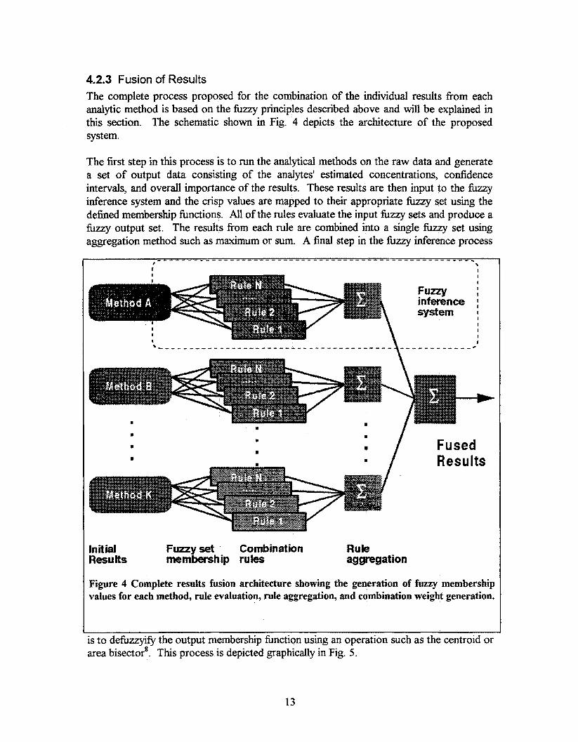
4.2.3 Fusion of Results The complete process proposed for the combination of the individual results from each analytic method is based on the hzzy principles described above and will be explained in this section. The schematic shown in Fig. 4 depicts the architecture of the proposed system.
The first step in this process is to run the analytical methods on the raw data and generate a set of output data consisting of the analytes' estimated concentrations, confidence intervals, and overall importance of the results. These results are then input to the fuzzy inference system and the crisp values are mapped to their appropriate fuuy set using the defined membership fbnctions. All of the rules evaluate the input fuzzy sets and produce a fi~zzy output set. The results from each rule are combined into a single fuzzy set using aggregation method such as maximum or sum. A final step in the kzzy inference process
I _ _ _ _ _ _ _ _ _ - - _ _ _ _ _ _ _ - - - - - - - - - - - - - - - - - - - - - - - - - - - - - - - - - -.
> I I
I I I
I Funy inference ; system I
I I
I I 1 I
8
a
a 8
m
8 / Fused Results
Initial Funy set Combination Rule Results membership rules aggregation
Figure 4 Complete resuits fusion architecture showing the generation of fuzzy membership values for each method, rule evaluation, rule aggregation, and combination weight generation.
is to defuzzyi@ the output membership hnction using an operation such as the centroid or area bisector'. This process is depicted graphically in Fig. 5.
13
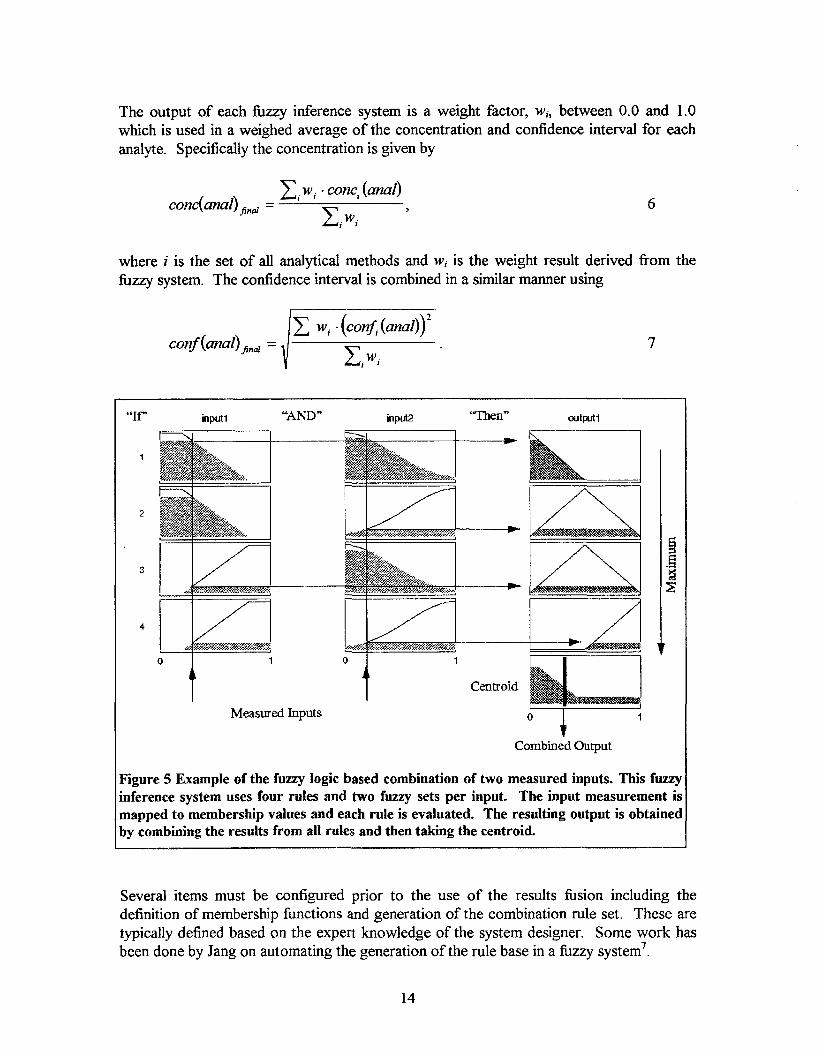
The output of each hzzy inference system is a weight factor, Wi, between 0.0 and 1.0 which is used in a weighed average of the concentration and confidence interval for each analyte. Specifically the concentration is given by
6
where z is the set of all analytical methods and Wi is the weight result derived from the hzzy system. The confidence interval is combined in a similar manner using
7
"If" input1 "AND" input2 'Then" output1
1
2
3
4
Combined Output
?igure 5 Example of the fuzzy logic based combination of two measured inputs. This fuzzy nference system uses four rules and two fuzzy sets per input. The input measurement i s napped to membership values and each rule is evaluated. The resulting output is obtained )y combining the results from all rules and then taking the centroid.
Several items must be configured prior to the use of the results h i o n including the definition of membership fimctions and generation of the combination rule set. These are typically defined based on the expert knowledge of the system designer. Some work has been done by Jang on automating the generation of the rule base in a hzzy system'.
14

4.3 Combination modes The DIM control and communication (CC) program implements four results combination modes in addition to the ability to select a single analytical method. The combination modes include unweighted mean, minimum, maximum, and fuzzy weighted mean. Each of these combination modes considers the concentration results from each available analytical method. The CC program generates a table of results as each analytical method is run with each row the results from a specific method and columns the concentration and confidence of each analyte and the overall importance measure for that method. This table is then used as the input to the combination module.
The unweighted average combination method generates a resulting analyte concentration by taking the arithmetic mean of each concentration column. Since the confidence interval is a measure similar to the standard deviation, the resulting confidence interval is the root mean square (RMS) of the individual measures. The unweighted average is given by Eq. 6 with wj equal to unity for all i and the confidence interval given by Eq. 7 with w, equal to unity.
The minimum and maximum combination modes generate the respective minimum or maximum concentration of all the computed concentrations for a given analyte. The confidence interval is obtained from the corresponding concentration (not the minimum or maximum contidence).
5. Software Structure As described in Section 2 the primary software modules in the DIM are the TSC-DIM communications interface, DIM-MATLAB interface, and analytical computatiorddata management. Each of these modules consists of either C/C* code or MATLAB code. The structure of the DIM sohare will be described in the following sections for each major fbnctional module. Each section will describe the components, which make up the overall hnctional module and the layout of the actual code.
5.1 DIM-SLM program The executable program dim-drn is the primary program of the DIM and it contains several source files. The main program file is “dim-slm.c” and the additional support files are “dim util.~,” dim-cmds.~,” and a header file “dim-s1m.h.” This program uses the generic 6M communications toolkit libraIy and thus consists of a main program, which calls the library function “Tkexecutive.” The remaining code consists of fbnctions that execute under specified TSC commands such as initialize, start, read, etc. One important attribute located in the main section of the code is the forking (or creation) of a child process which starts the program “matlab-eng.” Upon execution of the main program, the program splits and the child process starts the program which interfaces with the MATLAB processing engine and the parent process sets up communication with the “matlab-eng” program and then enters the toolkit executive.
The individual hnctions that are registered with the toolkit are dminit, dimstart, drmset, dimred, idle, bypass, intraLU0, and error. Most of the action is initiated via one of the
15
first four functions and most of the time is spent in the idle fbnction waiting for new commands or for commands to complete. A global variable, slmstate, is used to enable specific action to be taken within any of the above listed toolkit support hnctions. The variable can be set to the current action of the DIM when a command is started and cleared when the command completes. A typical execution of a TSC command would proceed in the following sequence:
(1) the appropriate action fbnction would be called (e.g. dimstart), (2) within the fbnction a message is generated and sent to the “matlab-eng”
program (if MATLAB processing is required to complete the action), (3) the fbnction sets the slmstate variable to indicate the processing state, (4) the idle function is entered and the message queue is checked to determine if
( 5 ) if a message is on the queue, the slmstate is set to “IDLE and the complete the MATLAB processing has completed,
message is returned to the TSC.
5.2 MATLAB-ENG program The executable program matlub-eng is a C program that interfaces between the dim-slm program and the MATLAB computational engine. This program links these two components in a non-blocking manner so that asynchronous communication can occur between the dim-slm program and the TSC. An additional layer of s o h a r e was required because the standard library hnction, which executes MATLAB code, blocks the calling program until the MATLAB code completes.
The matlab eng program utilizes message passing to receive commands and transmit results fiomko the dim-slm program. A MATLAB command string is generated by the dim - slm program and packaged into the body of a message and placed onto the queue. The matlab erzg program continually polls the receive message queue and parses commands when a message is received. A call to the MATLAB engine starts the desired processing. Once the dim slm program has sent the message it is free to listen for commands from the TSC and return messages from the muflub-eng program. When the MATLAB engine returns, the result is formatted into a message and sent to the dim - slm program.
The mutlubeng program thus runs in a continuous loop of waiting for a message to arrive, passing the message on to MATLAB, waiting for completion, sending the results out in a message. The messaging facility provides the capability for multiple messages to be stored in the queue and processed in a first in first out (FIFO) order.
5.3 MATLAB functions The analytical computation and some data management are performed by functions written in MATLAB. This computing environment enables robust and efficient algorithm development for analytical chromatogram processing. As described in the proceeding sections, the MATLAB hnction calls are formulated by the control and communication
16
program and passed to the MATLAB environment via the MATLAB interface program. The primary functions include chromatogram preprocessing, QA assessment, analytical methods, and results fusion. MATLAE3 functions are similar to other procedural languages with a calling format of “[outputl, output2, ... output n] =finction name (inputl, input2, . . . input n). Each of the finctions includes a description of the processing performed in the header area of the actual code.
6. Code modules The actual code listing for the “C” programs is included in Appendix D. A listing of the Makefile for the C programs is listed in Appendix E. The MATLAB fbnctions are listed in Appendix F.
17

7. Bibliography
[ 11 M. A. Abidi and R. C. Gonzalez, eds. Data Fusion In Robotics and Machine Intelligence, Academic Press, San Diego, CA, 1992.
[2] R. Bellman and M. Gertz. "On the analytical formalism of the theory of fuzzy sets," Information Sciences, 5: 149 - 156, 1973.
[3] 1. Bloch. "Information combination operators for data fusion: A comparative review with classification," IEEE Trans. on Sys., Man and Cybernetics - Part A: SYS. and H u I ~ ~ ~ s , 26(1): 52 - 67, 1996.
[4] J. W. Elling, L. N. Klatt, and W. P. U&. "Automated Data Interpretation in an Automated Environmental Laboratory," Laboratory Robotics and Automation, 6(2): 73 - 78, April 1994.
[ 5 ] T. H. Erkkila, R. M. Hollen, and T. J. Beugelsdijk. "The Standard Laboratory Module: An Integrated Approach to Standardization in the Analytical Laboratory," Laboratory Robotics and Automation, 6(2): 57 - 64, April 1994.
[6] Fung, L. W. and K. S. Fu. "The K* optimal policy algorithm for decision-making in fuzzy environments." Identification and System Parameter Estimation (P. Eykhoff, Ed.). North Holland, pp. 1025-1059, 1974.
[7] J.-S. R. Jang. "ANFIS Adaptive-Network-based Fuzzy Inference System," IEEE Trans. on Systems, Man, and Cybernetics, 23(3):665 - 685, 1993.
[8] A. Kandel. Fuzzy mathematical techniques with applications, Addison-Wesley, Reading, MA, 1986.
[9] L. F. Pau. "Sensor data fusion," Journal of Intelligent and Robotic Systems, 1 : 103 - 116,1988.
[lo] F. A. Settle, Jr., R. Hollen, and L. W. Yarbrough. "The Contaminant Analysis Automation Project:" American Laboratory, April 1995.
[ 1 11 M. A. Williams. "Application of artificial neural networks in the quantitative analysis of gas chromatograms". M.S. Thesis, University of Tennessee, Knoxville, TN, May 1996.
[12] R. R. Yager. "A general approach to the fusion of imprecise information," Intl. J. of Intelligent Systems, 12(1): 1 - 29, 1997.
18

[13] L. A. Zadeh. ” Fuzzy Sets and Applications: Selected Papers by L. A. Zadeh. John Wiley & Sons, New York, 1987.
[14] H. J. Zimmermann. Fuzzy Set Theory and Its Applications, 2nd ed. Kluwer Academic, Boston, 199 1.
19

Appendix A: Data fields for DIM sample processing
Field Number Contents ' 1.
1.
2.
3.
4.
5.
6 .
7.
8.
9.
10
11
Sample ID that is entered by the chemist with the HCI and transferred to the DIM by the TSC.
Sample type that is entered by the chemist with the HCI and transferred to the DIM by the TSC. Legal sample types are: standard, unknown, control, and blank.
Sample amount that is entered by the chemist with the HCI and transferred to the DIM by the TSC. The units on the sample amount are milligrams.
Filename of the AIA (netCDF) formatted data file for the sample. This filename will be passed to the DIM by the TSC with the extension ".CDF" or ".cdf". The DIM control sofhvare will create a second name using the original prefix with ".d" replacing the ".CDF" or ".cdf" extension. This resulting name will point to the subdirectory containing all the detailed information about the data processing applied to the sample.
The prefix of the filename of the calibration set information file. The DIM control software will obtain this filename during execution of the DIM. This field is included because of the probability of reanalyzing the sample(s) using a different calibration set information file.
Result of the signal on-scale QA evaluation. A value of 1 will denote the evaluation passed; a value of - 1 will denote the evaluation failed.
Result of the retention time QA evaluation. A value of 1 will denote the evaluation passed; a value of - 1 will denote the evaluation failed.
Result of the daily calibration standard QA check. A value of 1 will denote the evaluation passed, a value of -1 will denote the evaluation failed, and a value of 0 will denote this QA evaluation is not applicable to this sample.
The type of combination mode used in the result combination fuzzy logic system. The method of result combination will be fusion based upon the "importance" parameters.
The known amount of the surrogate standard in the sample in units of milligram. (The current contents of this field will be N.I., which means this functionality has not been implemented .)
The calculated recovery of the surrogate standard in the sample, expressed as a percent. (The current contents of this field will be N.I., which means this functionality has not been implemented.)
Name of analyte( 1).
12. Amount of analyte(1) in the sample with units of ppm.
13. Confidence interval on the amount of analyte( 1) with units of ppm.
14. Name of analyte(2).
15. Amount of analyte(2) in the sample with units of ppm.
16. Confidence interval on the amount of analyte(2) with units of ppm.
17. Name of analyte(3).
20

18. Amount of analyte(3) in the sample with units of ppm.
19. Confidence interval on the amount of malyte(3) with units of ppm.
21

Appendix B: DIM - TSC processing scripts
1. Introduction The following scripts are examples of possible sample processing sequences to be performed by the DIM SLM. Examples will be given for a standard sample flow, for a change in batch, and for several error conditions. Please refer to the "PCB DIM Command syntax" document for details on the actual commands.
2. Initialization sequence This operation would need to be performed once after the DIM SLM task is started. It may be run at any other time to bring the DIM SLM to a known default state.
TSC Command DIM Command INITIALIZE 000 ACK TO=20
SET PAR=COMB VAL=FUSION
SET PAR=BATCH-PATH VAL=/caa/data/oml2
100 COMPLETE RTN=O TXT="Initilization Complete" 000 ACK TO=5 100 COMPLETE RTN-0 TXT="set comb complete" 000 ACK TO=5 1 00 COMPLETE RTN=O TXT="set batchgath complete''
3. Batch processing of samples These operations would be performed during the routine operation of processing samples with the S A M system
TSC Command SET PAR=AIA-SAMP-TYPE VAL=UNKNOWN
SET PAR=AIA-SAMP--ID VAL=CO 184678
SET PAR=AIA-SAMP-AMT VAL="50.5 rng"
SET PAR=DATAFILE.-NAME VAL=ltmp/datalfile 1
START ACT=VALIDATE
START ACT=ANALYZE
SET PAR=AIA-SAMP-TYPE VAL=UNKNOWN
SET PAR=AIA-SAMP-ID VAL=CO 184679
SET PAR=AIA-SAMP-AMT VAL46.5
SET PAR-DATAFILE-NAME VAL=/tmp/datdfile2
DIM Command 000 ACK TO=5 100 COMPLETE RTN=O TXT="set aia-samp-type complete" 000 ACK TO=5 100 COMPLETE RTN=O TXT="set aia-samp-id complete" 000 ACK TO=5 100 COMPLETE RTN=O TXT="set aia-samp-amt complete" 000 ACK T0=5 100 COMPLETE RTN=O TXT="set datafile-name complete" 000 ACK TO=30 200 PROGRESS TO=30 200 PROGRESS TO=30 100 COMPLETE RTN=O TXT="validation complete" 000 ACK TO=60 200 PROGRESS T0=60 200 PROGRESS TO=60 100 COMPLETE RTN=O TXT="analyze complete" 000 ACK TO=5 100 COMPLETE RTN=O TXT="set aia-samp-type complete" 000 ACK TO=5 100 COMPLETE RTN-0 TXT="set aia-samp-id complete" 000 ACK TO=5 100 COMPLETE RTN=O TXT="set aia-samp-amt complete"
000 ACK TO=5 100 COMPLETE RTN=O TXT="set datafilename complete"
22

START ACT=VALIDATE
START ACT=ANALYZE
000 ACK TO=30 200 PROGRESS T0=30 200 PROGRESS TO=30 100 COMPLETE RTN=O TXT="validation complete" 000 ACK T0=60 200 PROGRESS TO=60 200 PROGRESS TO=4O 100 COMPLETE RTN=O TXT="analyze complete"
..... 4. New Batch processing of samples These operations would be performed immediately after the change from one batch to another.
TSC Command SET PAR=BATCH-PATH VAL=/caaldatalornl2
SET PAR=AIA-INJ-VOL VALz0.4
SET PAR=AIA_SAW-TYF'E VAL=UNKNOWN
SET PAR=AM-SAMP_ID VAL=CO 184679
SET PAR=AIA-SAMP-AMT VAb25.9
SET PAR=DATAFILE-NAME VAL=/tmp/data/file3
START ACT=VALLDATE
START ACT=ANALYZE
DIM Command 000 ACK TO=5 100 COMPLETE RTN=O TXT="set batchgath complete" 000 ACK TO=5 100 COMPLETE RTN=O TXT="set aia-inj-vol complete" 000 ACK T0=5 100 COMPLETE RTN=O TXT="set aia-samp-type complete" 000 ACK TO=5 100 COMPLETE RTN=O TXT="set aia-samp-id complete" 000 ACK TO=5 100 COMPLETE RTN=O TXT="set aia-samp-amt complete" 000 ACK TO=5 100 COMPLETE R T N 4 TXT="set datafile-name complete"
000 ACK TO=30 200 PROGRESS TO=30 200 PROGRESS TO=30 100 COMPLETE RTN=O TXT="validation complete" 000 ACK T0=60 200 PROGRESS TO=60 200 PROGRESS TO=60 100 COMPLETE RTN=O TXT="analyze complete"
23

5. Addition of standard to batch directory These operations would be performed whenever a new standard is added to the calibration set.
TSC Command SET PAR=BATCH-PATH VAL=/caa/data/oml2
SET PAR=AIA-INJ-VOL VAL=O.4
SET PAR=AIA-SAMP-TYPE VAL=STANDARD
SET PAR=AIA-SAMP-ID VAL=CO 184679
SET PAR=AIA-SAMPAMT VAL=0.004
SET PAR-D ATAFILE-NAME VAL=/tmp/data/file4
START ACT=ADD-STD
SET PAR=AIA-SAMP-TYPE VAL=STANDARD
SET PAR=AM-SAMP-ID VAL=CO 184662
SET PAR=AIA-SAMPAMT VAL=0.004
SET PAR=DATAFILE-NAME VAL=/tmp/data/fileS
START ACT=ADD-STD
....
.....
DIM Command 000 ACK TO=5 100 COMPLETE RTN=O TXT=“set batchgath complete” 000 ACK TO=5 100 COMPLETE RTN=O TXT=“set aia-inj vol complete” 000 ACK TO=5 100 COMPLETE RTN=O TXT=“set aia-samp-type complete” 000 ACK TO=5 100 COMPLETE RTN=O TXT=“set aia-samp-id complete” 000 ACK TO=5 100 COMPLETE RTN=O TXT=“set aia-samp-amt complete” 000 ACK TO=5 100 COMPLETE RTN=O TXT=“set datafile name complete” 000 ACK TO=30 200 PROGRESS TO=30 200 PROGRESS TO=30 100 COMPLETE RTN=O TXT=“Add Standard complete” 000 ACK TO=5 100 COMPLETE RTN=O TXT=“set aia-samp-type complete” 000 ACK TO=5 100 COMPLETE RTN=O TXT=“set aia-samp -id complete” 000 ACK TO=5 100 COMPLETE RTN=O TXT=“set aiasamp-amt complete” 000 ACK TO=5 100 COMPLETE RTN=O TXT=“set datafile name complete” 000 ACK TO=30 200 PROGRESS TO=30 200 PROGRESS TO=30 100 COMPLETE RTN=O TXT=“Add Standard complete”
(at the end of this cycle - 15 standards, the operator would be required to enter the DIM GUI and build the models for each method)
24
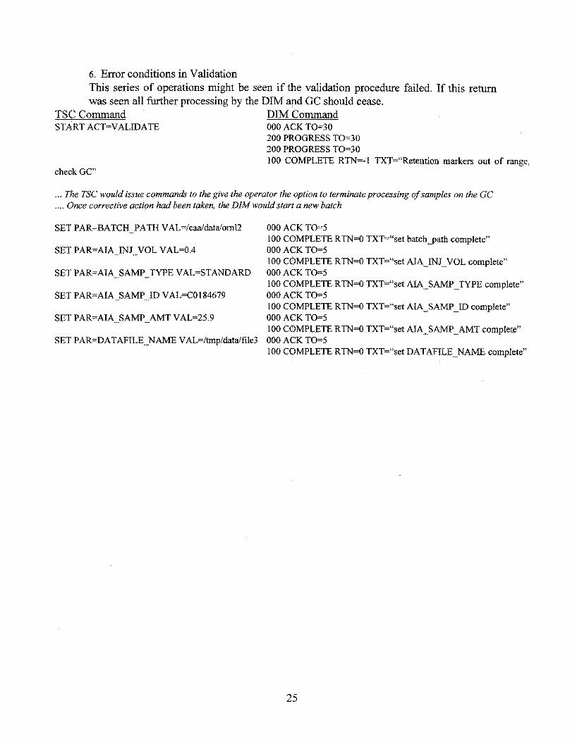
6 . Error conditions in Validation This series of operations might be seen if the validation procedure failed. If this return was seen all further processing by the DIM and GC should cease.
TSC Command DIM Command START ACT=VALIDATE 000 ACK T0=30
200 PROGRESS TO=30 200 PROGRESS TO=30 100 COMPLETE RTN=-1 TXT="Retention markers out of range,
check GC"
... The TSC would issue commands to the give the operator the option to terminate processing of samples on the GC
..._ Once corrective action had been taken, the DIM would start a new batch
SET PAR=BATCH-PATH VAL=/caddatdornl2 000 ACK T0=5 100 COMPLETE RTN=O TXT="set batchgath complete"
SET PAR=AIA_INJ-VOL VAL=O.4 000 ACK T0=5 100 COMPLETE RTN=O TXT="set AIA-INJ-VOL complete"
SET PAR=AIA-SAMP-TYPE VAL=STANDARD 000 ACK T0=5 100 COMPLETE RTN=O TXT="set AIA-SM-TYPE complete"
SET PAR=AIA-SAMP-ID V A L 4 0 184679 000 ACK T0=5 100 COMPLETE RTN=O TXT="set AIA-SAM€-ID complete"
SET PAR=AIA-SAMP-AMT VAL=25.9 000 ACK T0=5 100 COMPLETE RTN=O TXT="set AIA-SAMP-AMT complete"
SET PAR=DATAFILE-NAME VAL=/tmp/data/file3 000 ACK T0=5 100 COMPLETE RTN=O TXT="set DATAFILE-NAME complete"
25

Appendix C: ASCII results file
062502 unknown 1.000e+03 /mt/CAA/output/062502.cdf 425460 1 1 0 3 1.600e- 01 1.048e02 1242 4.024e-01 2.987e-02 1254 1.434e-01 4.658e-02 1260 9.573e-03 3.520e-02 062503 unknown 1.000e+03 /mnt/CAA/output/062503.~df 425460 1 1 0 3 1.600e- 01 1.067e+02 1242 1.207e-02 2.018e-02 1254 3.865e-01 3.728e-02 1260 9.015e-03 3.543e-02 062504 unknown 1.000e+03 /mnt/CAA/output/062504.~df 425460 1 1 0 3 1.600e- 01 1.018e+02 1242 -4.555e-03 1.329e-02 1254 1.455e-02 2.392e-02 1260 3.559e-01 3.295e-02 06272 1 unknown 1.000e+03 /mnt/CAA/output/O62721 .cdf 425460 1 1 0 3 7.200e- 02 1.153e+02 1242 -1.207e-02 9.304e-03 1254 2.215e-02 1.744e-02 1260 4.300e-02 9.933e-03 072309 unknown 1.000et-03 /mnt/CAA/output/O72309.~df 425460 1 1 0 3 1.600e- 01 1.748e+01 1242 4.723e-02 3.456e-02 1254 7.652e-02 4.867e-02 1260 -1.027e-02 3.222e-02 072503 unknown 1.000et-03 /mnt/CAA/output/072503.~df 425460 1 1 0 3 1.600e- 01 4.180e+01 1242 1.357e-01 3.481e-02 1254 2.172e-01 4.748e-02 1260 8.249e-02 3.649e-02 072505 unknown 1.000e+03 /mnt/CAA/output/072505.cdf 425460 1 1 0 3 1.600e- 01 3.692e+01 1242 1.003e-01 3.366e-02 1254 1.887e-01 4.079e-02 1260 3.572e-02 3.965e-02 072506 unknown 1.000e+03 /mnt/CAA/output/072506.~df 425460 1 1 0 3 1.600e- 01 3.433et-01 1242 1.224e-01 3.399e-02 1254 2.188e-01 4.165e-02 1260 4.633e-02 6.267e-02 072507 unknown 1.000e+03 /mnt/CAA/output/072507.cdf 425460 1 1 0 3 1.600e- 01 1.443e+01 1242 7.141e-02 3.735~~-02 1254 1.149e-01 4.460e-02 1260 3.049e-02 6.064e-02 072508 unknown 1.000e+03 /mnt/CAA/output/072508.~df 425460 1 1 0 3 1.600e- 01 1.452e+01 1242 3.91Se-02 3.331e-02 1254 8.874e-02 4.209e-02 1260 1.708e-02 2.856e-02
26

Appendix D: "C"Code listings aia2oke.c
/* int aiaqoke(char *filename, char *type-Val, float amt-Val) Inputs:
filename - a string of the pathname to the netCDF AIA file in
type-Val - an ASCII string value indicating the sample type.
amt-val- a floating point value representing the amount of sample
which to poke the type and amount volume data.
This will be poked into the GLOBAL attribute "sample-type"
in mg outputs:
Error code representing the status of the function call, negative value indicates failure, zero success
Compile with ANSI C compiler.
Modifications by MAH 6/4/96 - changed sample-amount to float argument (was char) added int error code return with associated checks
Modifications by MAH 8/1/96 - changed to aiaqoke, removed injection volumn
"/ #define NO-SY STEM-XDR-INCLUDES #define NO-GETPID #define USE-XDRNCSTDIO
#include <stdio.h> #include <string.h> #include <stdlib.h> #include "array.c" #include I'attr.c" #include "cdf.c" #include "dim.c" #include "error.c" #include "fi1e.c" #include "g1obdef.c" #include "iarray.c" #include 'lputget.c" #include "putgetg.c" #include "sharray.c" #include "string.c" #include "var.c"
/* Needed for strtod() and malloc() */
#include <sys/types.h>
27

#include <types.h> #include <xdr.h> #include "xdr . c #include "xdrstdio.c" ##include "xdrfloat.c"
int aiaqoke(const char *cdfname, char *type-Val, float amt-Val)
{ int cdfid; int len; int ecode; double *amount; /* Declare pointer to amount value */
/* Declare file ID */ /* Declare length variable */
/* return error code */
cdfid=ncopen(cdhame,NC-WTE); /* Open netCDF file and assign ID#*/ if(cdfid = -1) { /* Open error */
fprintf(stderr, "Could not execute ncopen (aiagoke) on file: %s.\n"); return(- 1);
I ecode = ncredef(cdfid); if(ecode == -1) {
fprintf(stderr, "Could not execute ncredef (aiaqoke).\n"); return(ecode);
/* Open in define mode */ /* Check return code */
1
ecode = ncattput(cdfid,NC-GLOBAL,"sample-type",NC - CHAR,\ strlen(type-Val)+ 1 ,type-Val);
if(ecode = -1) { fprintf(stderr, "Could not execute ncattput, samp-type (aiagoke).\n"); return( ecode);
/* Check return code */
1
len= 1 ; amount = malloc(sizeof(doub1e)); if(amount == (double *) NULL) {
/* Number of double values*/ /* Allocate space for double */
fprintf(stderr, "Could not malloc memory (aiaqoke).hn"); return(- 1);
1 if( amt-Val != 0.0) {
*amount = (doub1e)amt-Val; fprintf(stderr,"Double sample amount vaiue:%l 1 g\n",*amount); ecode = ncattput(cdfid,NC_GLOBAL,"sample_ainount",NC_DOUBLE,len,amount); if(ecode = - 1) {
fprintf(stderr, "Could not execute ncattput, smp-amt (aiagoke).\n"); return(ecode);
/* Check return code */
1 1
28

ecode = ncendef(cdfid); if(ecode == - I) {
fprintf(stderr, "Could not execute ncended (aia_poke).\n"); return(ecode) ;
/* End define mode */ /* Check return code */
1
ncclose(cdfid); /* Close netCDF file*/
free(amount);
return(0);
1 dim-cmds.c #include "dim-s1m.h"
int init-cmd( Dim-stateP stateP) {
char *cptr; char complete[BUFSIZ+l]; char errmsg@UFSIZ+l]; char ack[4O]; int i j ;
#ifdef DEBUG
#endif +rintf(stderr, "Initialize Command\n");
/* code to initialize state of DIM follows */ init-state( stateP); print-state( stateP);
return( 0); 1
int read-cmd( char *buf, int server, Dim-stateP stateP)
{
char *cptr, *valcptr; char complete[BUFSIZ+l]; char emsg[BUFSIZ+l]; char ack[40];
#ifdef DEBUG
29

fprintf(stderr, "Read Command\n"); #endif
if( (cptr = strtok( buf, I' ") ) != NULL ) { I* first thing to do is acknowledge command *I
sprintf(ack, "000 ACK TO=10 KEY=%s\O",buf); CMsendMessage( server, ack);
I* code to read state of DIM follows *I if((cptr=strtok(NULL," ")) != (char *)NULL) { I* gets parameter to set*/
fprintf(stderr,"Read parameter: %s\n",cptr); if(read-state(stateP, cptr, enmsg) != 0) {
sprintf(enmsg, "Error in Read"); sprintf(complete, 'I 100 COMPLETE RTN=%d KEY=%s TXT=%s", - 1, buf, errmsg); CMsendMessage( server, complete);
1 else { I* sprintf(errmsg, "Read sucessful"); */
sprintf(complete, 100 COMPLETE RTN=%d KEY=%s TXT=%s", 0, buf, errmsg); CMsendMessage( server, complete);
I } else {
sprintf(emnsg, "No Read parameter"); sprintf(complete, "1 00 COMPLETE RTN=%d KEY=%s TXT=%s", - 1, buf, e m s g ) ; CMsendMessage( server, complete);
) else { I* invalid command */ sprintf(ermsg, "Invalid command '%os", buf); sprintf(complete, 'I 100 COMPLETE RTN=%d KEY=%s TXT=%s", - 1, buf, errmsg); CMsendMessage( server, complete);
1 3
int start-val-cmd( char *buf, int server)
1
char *cptr; char complete[BUFSIZ+l]; char emsg[BUFSIZ+l]; char ack[40];
#ifdef DEBUG
#endif fprintf(stderr, "Start Validate Commandh");
if( (cptr = strtok( buf, I' ") ) != NULL ) { /* first thing to do is acknowledge command */
30

sprintf(ack, "000 ACK TO=30 KEY=%s\O",buf); CMsendMessage( server, ack);
1" code to validate chromatograms follows */
sprintf(complete, I' 100 COMPLETE RTN=%d KEY=%s TXT=%s", 0, buf, emnsg); CMsendMessage( server, complete);
} else { I* invalid command *I sprintf(errmsg, "Invalid command %s", buf); sprintf(complete, I' 100 COMPLETE RTN=%d KEY=%s TXT=%s", - 1 , buf, e m s g ) ; CMsendMessage( server, complete);
I 1
int start_ana-cmd( char *buf, int server) {
char "cptr; char complete[BUFSIZ+l]; char emsg[BUFSIZ+I]; char ack[40];
#ifdef DEBUG
#endif fprintf(stderr, "Start Analyze Commandh");
if( (cptr = strtok( buf, I' ") ) != NULL ) { /" first thing to do is acknowledge command *I
sprintf(ack, "000 ACK T0=3 0 KEY=%s\O",buf); CMsendMessage( server, ack);
/* code to validate chromatograms follows */
1 else { /* invalid command *I sprintf(emnsg, "Invalid command %s", buf); sprintf(complete, "1 00 COMPLETE RTN=%d KEY=%s TXT=%s", -1 , buf, e m s g ) ; CMsendMessage( server, complete);
1 1
31

int abort-cmd( char *buf, int server, Dim-stateP stateP)
{
char *cptr; char complete[BUFSIZ+l]; char errmsg[BUFSIZ+l]; char ack[40];
#ifdef DEBUG
#endif fprintf( stderr, "Abort Commandh");
if( (cptr = strtok( buf, 'I) ) != NULL ) { /* first thing to do is acknowledge command */
sprintf(ack, "000 ACK TO=10 KEY=%s\O",buf); CMsendMessage( server, ack);
fprintf( stderr, "Aborting operation and re-initializingh"); init-state( stateP); print-state( stateP); sprintf(errmsg, "Abort complete"); sprintf(complete, I' 100 COMPLETE RTN=%d KEY=%s TXT=%s", 0, buf, errmsg); CMsendMessage( server, complete);
sprintf(errmsg, "Invalid command '%OS", buf); sprintf(complete, "1 00 COMPLETE RTN=%d JSEY=%s TXT=%s", - 1, buf, errmsg); CMsendMessage( server, complete);
/* code to initialize state of DIM follows */
1 else { /* invalid command */
1 1
int status-cmd( char *buf, int server, Dim-stateP stateP)
{
char kptr; char complete[BUFSIZ+l]; char errmsg[BUFSIZ+ 1 1; char ack[40];
#ifdef DEBUG
#endif @rintf(stderr, "Status Commandh");
if( (cptr = strtok( buf, ") ) != NULL ) { /* first thing to do is acknowledge command */
sprintf(ack, "00 1 IACK RTN=O KEY=%s\O",buf); CMsendMessage( server, ack);
32

/* code to initialize state of DIM follows */ print-state( statep); sprintf(emnsg, "Status complete"); sprintf(complete, 'I 100 COMPLETE RTN=%d KEY=%s TXT=%s", 0, buf, errmsg);
/* CMsendMessage( server, complete); */ 1 else { /* invalid command */
sprintf(errmsg, "Invalid command %s", buf); sprintf(complete, 'I 100 COMPLETE RTN=%d KEY=%s TXT=%s", - 1, buf, enmsg);
/* CMsendMessage( server, complete); */ 1
1
dim-s1m.c
#include <stdio.h> #include <string.h> #include <ctype.h> #include <time.h> #include <sys/types.h> #include <sys/ipc.h> #include <sys/msg.h> #include <sys/shm.h> #include <signal.h> #define CMLXB #include " tkapi . h " #include "d im-s Im . h "
int getstdin( char "buffer ); int processkeys( char *buffer);
/* command call back prototypes "/
int diminit( int chan ); int dimstart( int chan ); int dimset( int chan ); int dimread( int chan ); int comStatus( int type, char *message );
struct TKcmd slmCmds[] = { { "initialize", diminit } 2
{ "start", dimstart >, { %et", dimset ), { "read", dimread } , { NULL, NULL ) f ;
int slmstate=IDLE; time-t slmstop;
33

time-t nextprog; int extime; iiit exlevel; Dim-state state; Dim-stateP stateP;
int tmsqid; /* returned send message queue id */ int rmsqid; /* returned receive message queue id */ int shmid; /* returned shared memory id */
Engine *ep; char *mat-output;
/* initalize variables */
char "datatosend = "This is suppose to be data";
int diminit( int chan ) {
int i; int ret; char errtxt[LBUFF-SIZE+l];
TKAck( 5 , -1);
ret = init-state(stateP);
if (ret = 0) {
1 ret = print-state(stateP);
slmstate = IDLE;
if(ret < 0) { /* error condition */ dim-err_code(ret, errtxt); TKComplete( 0, errtxt, -1 );
strcpy(errtxt,"Initialization successful"); TKComplete( 0, entxt, - 1 );
1 else {
1
return TK-CONTINUE; 1
int dimstart( int chan ) {
34

int ret;
char errtxt[LBUFF-SIZE+I]; char cmdstring[LBUFF-SIZE+ 11;
' char *action;
TKAck( 120, - 1);
ret = 0;
if(!TKGetString("act",&action)) { /* error return */ return TK-CONTINUE;
1
I* check for entries in the required fields of the state table *I
if((ret = check-state(stateP)) < 0) { I* error condition */ dim-err-code(ret, entut); f'printf( stderr, "%s.\n",errtxt); ret = -1; TKComplete( ret, entut, -1 ); return TK-CONTINUE;
1
I* perform action *I fprintf(stderr,"Action code:%s.\n",action); if(strcasecmp(action, "add_std")==O) {
slmstate = ADDSTD; fprintf(stderr,"Start add standard\n"); sprintf(errtxt, "Successful %s 'I , action); slmstate = IDLE;
} else if (strcasecmp(action, "validate")=O) { slmstate = VALIDATE; fprintf(stderr,"Start validate h"); if((ret = validate(stateP)) 0) { I* error condition *I
strcat(errtxt, decipher-err-codes(ret, 1)); strcat(errtxt, decipher_err-~odes(ret,2)); fprintf( stderr, "%s.\n",errtxt);
sprintf(errtxt, "Successful %s 'I, action);
} else if (strcasecmp(action, "analyze")==O) {
} else {
1
slmstate = ANALYZE; fprintf(stderr,"Start analyze \n"); if((ret = analyze(stateP)) < 0) { I* error condition */
strcat(errbit, decipher-err-codes(ret, 1)); strcat(errtxt, decipher_err_codes(ret,2)); fprintf(stderr,"%s.\n",errtxt);
35

} else {
I sprintf(errtxt, "Successful %s 'I, action);
fprintf(stderr,"Bad action code \n"); dim-err-code(BAD-ARG, errtxt); ret = -1;
sprintf(errtxt, "Successful %s ", action);
} else {
1
if (slmstate == IDLE) { TKComplete( ret, errtxt, - I );
1
return TK-CONTINUE; 1
int dimset( int chan ) {
char *par, *Val; char errtxt[LBUFF-SIZE+ 11; int rtn-code;
T u c k ( 30, - 1);
if( !TKGetString("par",&par)) { /* error return */ fprintf(stderr,"Error in Set,Parameter code:empty.\n"); return TK-CONTINUE;
1 if( !TKGetString("val",&val)) { /* error return */
fprintf(stderr,"Error in Set,Parameter code:%s, value:empty.\n",par); return TK-_CONTINUE;
1 rtn-code = set-state(stateP, par, Val); if(rtn-code < 0) {
fprintf(stderr,"Error in Set, Parameter code:%s, value:%s.b",par,vaI); sprintf(errtxt,"Error in Set,Parameter code:%s, value:%s.",par,val); rtn-code = - 1 ;
fprintf(stderr,"Warning in Set,Parameter code:%s, value:%s.\n",par,val); print-state( stateP); sprintf(errtxt, "Set %s = %s complete with warning! ",par,val); rtn-code = 1;
fprintf(stderr,"Set %s = %s\n", par, Val); print-state( stateP); sprintf(errtxt, "Set %s = %s complete",par,val); rtn-code = 0;
} else if (rtn-code >O) { /* warning */
} else {
36

1
if (slmstate == IDLE) { TKComplete( rtn_code, errtxt, - 1 );
1 return TK-CONT'INUE;
1
int dimread( int chan ) {
char *par; char errtxt[LBUFF-SSZE+l]; int rtn-code;
T u c k ( 5, -1);
if(!TKGetString("par",&par)) { /* error return */ fprinff(stderr,"Error in Read, Parameter code:empty .\n"); return TK-CONTINUE;
1 if(read-state(stateP, par, errtxt) != 0) {
@rintf(stderr,"Error in Read, Parameter code:%s.'m",par); sprintf(errtxt,"Error in Read,Parameter code:%s",par); rtn-code = - 1 ;
rtn-code = 0; 1 else {
1
TKComplete( rtn-code, errtxt, - 1 ); return TK-CONTINUE;
1
int idle( long runtime )
char buffer[BUFSIZ+l 1; Rtn-msgbuf rmsgbuf; /* message send structure */ Rtn-msg-bufP rmsgp;
FILE * res-fid; float recovery; char res-fname[LBUFF-SIZE] ; char errtxt[LBUFF-SIZE+ I];
long msgtyp;
rmsgp = &rmsgbuf;
37

if( getstdin( buffer ) == 1) switch( processkeys( buffer ) )
case SEm-COMMAND: t
TKsendMessage( buffer ); break;
TKsendData( (void *)datatosend, strlen(datat0send) + 1 ); break;
case SEND-DATA:
case QUIT-COMMAND: return TK-STOP;
case SEND-QUERY: break;
TKQuety("What do I do now?", "eat work", - 1 ); break;
1
switch( slmstate ) {
case ADDSTD: break;
case VALIDATE: /* receive message from matlab engine process */
msgtyp = 0; if(msgrcv(rmsqid, rmsgp, MSG-SIZE, msgtyp, IPC-NOWAIT)>=O) {
printf("\nresponse from peer receivedh"); slmstate = IDLE;
/* set appropriate flags */ if (rmsgp->code = 0) {
fprintf(stderr, "Matlab call successfulh"); if (strcasecmp(stateP->samp-type, ''control'') == 0) {
} else { stateP->qa-cal-flag = 1 ;
sscanf(rmsgp->result,"%g",&recovery); state€'->sunrecover = recovery; stateP->qa-sur-flag = 1 ;
1 TKComplete( rmsgp->code, "Validate complete", - 1 );
strcat(errtxt, decipher-err-codes(rsgp->code, 1 )); strcat(errtxt, decipher-err-codes(rmsgp->code,2)); fprintf( stderr, "%s .\n",errtxt); fprintf(stderr, "Matlab call error\n"); if (strcasecmp(stateP->samp-type, "control") == 0) {
} else {
} else {
stateP->qa-cal-flag = - 1 ;
sscanf(rmsgp->result,"%g",&recovery); state€'->surr-recover = recovery; stateP->qa-sur-flag = - 1 ;
38

1 TKComplete( rmsgp->code, e m t , - 1 );
1 /* write results to ASCII results file */
strcpy(res-fname,stateP->batch_path); strcat(res-fname,"/"); strcat(res-fname, RESULTS-FILE); fprintf(stderr,"results file: %shn",res-fname); if((res-fid = fopen(res-fname, "a+")) = (FILE *)NULL) {
fprintf( stderr,"Could not open %s to append results\n",res - fname); fprintf( stderr,"Exiting ! !\n");
return TK-STOP; I fseek(res-fid, OL, SEEK-END); fprintf(res-fid,"%s ",stateP->samp-id); fprintf(res-fid,"%s I',stateP->samp-type); fprintf(res-fid,"%- 10.3 e ",stateP->samp-amt); fprintf(res-fid,"%s ",stateP->datafile); fprintf(res-fid,"%s ",stateP->calib-set); fprintf(res-fid,"%- 3i ",stateP->qa-scale-flag); fprintf(res-fid,"%- 3i ",stateP->qa-&-flag); fprintfiires-fid,"%- 3i ",stateP->qa-cal-flag); fprintf(res-fid,"%- 3i ",stateP->comb-mode); fprintf(res-fid,"%- 10.3e ",stateP->sun- - amt); fprintf(res-fid,"%- 10.3e ",stateP->sm-recover); fprintf(res-fid, Yri");
/* insert newline for all but type unknown or if qc check failed*/ /*
if (strcasecmp( stateP->samp-type, "unknown") ! = 0 I I (rmsgp->code = 0)) { fprintf(res-fid, '%I");
I
fclose( res-fid); */
1 break;
case ANALYZE: msgtyp = 0; if(msgrcv(rmsqid, rmsgp, MSG-SIZE, msgtyp, IPC-NOWAIT)>=O) {
printf("\nresponse from peer received\n"); slmstate = IDLE; if (rmsgp->code = 0) {
TKComplete( rmsgp>code, rmsgp->result, - 1 ); fprintf(stderr, "Matlab call successful\n");
fprintf(stderr, "Matlab call error\n"); strcat(errtxt, decipher-err-codes(rmsgp->code, 1)); strcat(entxt, decipher~err~codes(rsgp->code,2)); fprintf( stderr,"%s.\n",errtxt);
1 else {
39

TKComplete( rmsgp->code, errtxt, -1); ) strcpy( res_fname,stateP->batchjath); strcat(res-fname,tl/l'); strcat(res-fname, RESULTS-FILE); fprintf(stderr,"results file: %s\n",res-fname); if((res fid = fopen(res-fname, "a+")) = (FILE *)NULL) {
fprinif(stderr,"Could not open %s to append results\n",res-fname); fprintf(stderr,"Exiting ! !\n");
return TK-STOP;
fseek(res-fid, OL, SEEK-END); fseek(res-fid, - lL, SEEK-CUR); /*remove newline from validate*/ fprintf(res-fid, "%s\n",rmsgp->result); fclose(res-fid);
1 /* reset state */
sprintf( stateP->samp-type, DEF-S AMP-TYPE); sprintf(stateP->samp-id, DEF-SAMP-ID); sprintf(stateP->datafile, DEF-DATAFILE); stateP->surr-recover = DEF-SUR-RECOVER; stateP->samp amt = DEF-SAMP-AMT; stateP->qa-scile-flag = DEF-QA-SCALE; stateP->qa-rt-flag = DEF - - QA RT; stateP->qa-cal-flag = DEF-QA-CAL; stateP->qa-sur-flag = DEF-QA-SUR;
break; case SET-BATCH:
msgtyp = 0; if(msgrcv(rmsqid, rmsgp, MSG-SIZE, msgtyp, IPC-NOWAIT)>=O) {
printf("hresponse from peer received\n"); slmstate = IDLE; if (rmsgp->code == 0) {
fprintf(stderr, "Matlab call successfulh"); TKComplete( rmsgp->code, "Set Batch Path complete", - 1 );
fprintf(stderr, "Matlab call errorb"); strcat(errtxt, decipher-err_codes(rmsgp->code, 1)); strcat(errtxt, decipher-err_codes(rmsgp->code,2)); fprintf( stden^,"%s.h",e~t); TKComplete( rmsgp->code, errtxt, -1 );
) else {
1 1
break; case IDLE:
msgtyp = 0;
40

if(msgrcv(rmsqid, rmsgp, MSG-SIZE, msgtyp, IPC-NOWAIT)>=O) { printf("\nresponse from peer received\n"); if (rmsgp->code = 0) {
} else { fprintf(stderr, "Matlab call successfulh");
fprintf(stderr, "Matlab call errorh");
1 1
break;
return TK-CONTINUE; 1
1
int bypass( char *channel, char *cmdstring ) {
char errtxt [LBUFF-S IZE+ 1 3 ; int rtn_code=O; Cmd-msg-buf tmsgbuf; I* message send structure *I Cmd-msg-buff tmsgp; int msgsz, msgflg; long m s m ;
struct msqid-ds tmsgds; struct msqid-ds *tmsgdsp; struct msqid-ds rmsgds; struct msqid-ds *rmsgdsp; struct shmid-ds shmds; struct shmid-ds *shmdsp;
tmsgp = &tmsgbuf; tmsgdsp = &tmsgds; rmsgdsp = krmsgds; shmdsp = &shmds;
tmsgp->mtype = 1; msgflg = 0;
printf("bypass- %s %s\n", channel, cmdstring );
stmcpy(tmsgp->command, cmdstring, LBUFF-SIZE-2);
msgsz = strlen(cmdstring) -t 1;
I* *I I* send message to queue I* *I m-code = msgsnd(tmsqid, tmsgp, msgsz, msgflg); if (rtn-code = -1) {
*I
41

perror("msgop: msgsnd failed"); sprintf(entxt, "Message send failed, in Bypass");
1
sprintf(errtxt, "Message sent to process running MATLAB engine");
msgctl(tmsqid, IPC-STAT, tmsgdsp); msgctl(rmsqid, IPC-STAT, rmsgdsp); shmctl(shmid, IPC-STAT, shmdsp);
fprintf( stderr,"number of messages on transmit que:%d\n",tmsgdsp->msg-qnum); fprintf(stderr,'humber of messages on receive que:%d\n",rmsgdsp->msg qnum); fprintf(stderr,'lnumber of shared memory attachments:%d\n",shmdsp->scm - nattch);
slmstate = IDLE;
TKJAck(rh.l-code, errtxt );
return TK-CONTINUE; 1
int intraLUO( int cmd, int channel ) {
char responsetxt[ 1281; char *response;
printf("intraLU0 - %d %d\n", cmd, channel); switch( cmd ){
case ABORT-CMD: TKsend( 1, "%dRTN", 0 , "KEY ,"ABORT","TXT", "Aborting DIM processing", 0 ); slmstate = IDLE;
break;
if( TKGetString( "txt", &response ) )
TKIAck( 0, NULL ); break;
case STATUS-CMD: if( slmstate == IDLE ) {
TIUAck( 0, "IDLE" );
case REPLY-CMD:
printf("Response = %s\n", response );
print-state( stateP); } else {
sprintf( responsetxt, "%s", TKgetLastCommandO ); TKIAck( 0, responsetxt );
1
break;
42

1 return TK-CONTINUE;
1
int error( int error ) 1
1 return TK-ABORT;
int cornStatus(int type, char *message) {
switch(type) { case SERVER-CONNECTED:
printf("S1ERVER CONNECTED "); break;
printf( "CONNECTION DISCONNECTED 'I); break;
printf("BR0ADCAST MESSAGE "); break;
case CONNECTION-DISCONNECTED:
case BROADCAST-MES SAGE:
I printf(message); printf( "\r\n"); return TK-CONTINUE;
}
main( argc, argv ) int argc; char *argv[];
char *myname; char *portnum; int theserver = - 1 ; int len, ret; struct TKcmd *cmdtab = slmCmds; char matlab-strt[LBUFF-SIZE]; int mat-out-size = MATLM-OUTPW-SIZE;
I* pointer to name of program */ I* pointer to remote user name */
keY-t tkey; I* unique key for send message queue */ keY-t rkey; I* unique key far receive message queue */ int cldgid; /* child pid */
myname = argv[O];
43

I* Check that there is one command line argument *I
if( (argc < 4 ) ( argc > 5 ) ) { fprintf( stderr, "Usage: %s slmid service broadcastport \n", myname ); fprintf( stderr, "OR\n"); fprintf( stderr, "Usage: %s slmid service host port\n", myname ); exit( 1);
I
I* set the urnask mode */ umask(07); I* no other permission, user and group as requested *I
switch ((cldqid=fork())) { case -1: I* error *I
perror( "main: fork"); exit( 1);
execl("matlab-engl', "matlab-eng", (char *) NULL); perror( "main:execl"); exit( 1);
break;
case 0: 1" child *I
case 1: I* parent *I
I
I* set up message queues and shared memory *I
/* *I
I* *I tkey = ftok("/usr", 'A'); rkey = ftok( "/usr", 'B');
I* generate keys based on file and code *I
if(rkey == -1 tkey = -1) { fprintf( stderr,"ftok failure in ?'OS, exiting\n",argv[O]); exit( 1);
1
I* *I /* create the message channel I* *I
*I
if ((tmsqid = msgget(tkey, (IPC-CREAT I 0666))) = - 1) { perror("msgget: msgget failed"); exit( 1);
1
44

if ((rmsqid = msgget(rkey, (IPC-CREAT I 0666))) = -1) { perror("msgget: msgget failed"); exit( 1);
1
I* *I
I* *I if ((shmid = shmget(tkey, 600000, (IPC-CREAT I 0666))) == -
1) perror("shmget: shmget failed"); exit( 1);
/* create shared memory segment *I
1
stateP = &state;
TKSetSLMinfo( "dim", argv[ 13, "ORNL", 1, "Ver. 1 .O" );
if( argc == 4 ) TKSetConBroadcast( argvC21, atoi( argv[3] ) );
else TKSetConDirect( argv[2], argv[3], atoi( argv[4] ) );
init-state( stateP);
ret = TKexecutive( &slmCmds[O], idle, bypass, intraLU0, error, comStatus, 0 );
I* remove message queues and shared memory */ msgctl(tmsqid, IPC-RMID, (struct msqid-ds *) NULL); msgctl(msqid, I P C - M D , (struct msqid-ds *) NULL); shmctl(shmid, IPC-RMID, (struct shmid-ds *) NULL);
I* kill child process *I if(kill(cld_pid, SIGKILL))
perror("kil1: kill child failed");
switch (ret ){ case TK-ABORT:
printf( "Error in TKExec - %s\n", TKgetLastErrorO); printf(" Abortingb"); exit( 1); break;
case TK-STOP:
45

printf( "Stopping\n");
break; exit( 0);
1
dim s1m.h #ifndef -DIM-SLM- #define DIM-SLM-
#include <stdlib.h> #include <stdio.h> #include <string.h> #include <un i st d . h> #include <signal.h> /*#include "cmapi.h"*/ #include "engine.h"
#define LBUFF-SIZE 490 #define MSG-SIZE 500 #define RESULTS-FILE "results.txtr'
typedef struct dim-state { int comb-mode; /* results combination mode *I char batchqath[LBUFF-SIZE]; /* complete pathname to base level of batch */ char samp-type[LBUFF-SIZE]; char samp-id[LBUFF-SIZE]; char datafile[LBUFF-SIZE]; /*full base pathname of raw chromatogram */
float inj-vol; float samp-amt; float surr-amt; float surr-recover; char calib - set[LBUFF-SIZE]; /* prefix of the filename of the cal set */ char sum-set[LBUFF-SIZE]; /* prefix of the filename of the surrogate set*/ int qa-scale-flag; /* results of qa off-scale signal check*/ int qa-rt-flag; /* results of qa retention time check */ int qa-sur-flag; I* results of surrogate recovery check *! int qa-cal-flag; /* results of qa calibration check */
/* sample type AIA header */ /* sample id AIA header */
/* and ASCII peak area file */ /* injection volume in uL*/
/* sample amount in mg */ /* surrogate amount in ng */
/* surrogate recovery in percent "1
] Dim-state;
typedef struct dim-state *Dim - stateP;
typedef struct cmd-msg-buf { long mtype; char command[LBUFF - SIZE];
/* message type */ /*MATLAB command string */
46

1 Cmd-msg-buf;
typedef struct cmd-msg-buf *Cmd-msg-bufP;
typedef struct rtn-msg-buf { long mtype; /* message type */ int code; /* variable code from matlab environemnt */ char result[LBUFF-SIZE]; /*MATLAB command string */
] Rtn-msg-buf;
typedef struct rtn-msg-buf *Rtn_msg-bufP;
int getstdin( char *buffer ); int processkeyin( char *buffer); int processcmds( char *buf ); int init-state(Dim-stateP statep); int set-state(Dim-stateP stateP, char "paramcptr, char "valcptr); int read-state(Dim-stateP stateP, char *paramcptr, char *valcptr); int print-state(Dim-stateP stateP); void iluo-action(); int aiaqoke(const char *cdfname, char *type-Val, float amt-Val); void dim-err-code(int err-no, char "buffer); int check-state(Dim-stateP stateP); int validate(Dim-stateP stateP); char *decipher-err-codes(int, int); extern void exit();
extern char *malloc(); extern char *shmat();
extern void perror0;
#define MATLAB-OUTPUT-SIZE 20000
enum { NO-COMMANJl= 0, SEND-COMMAND, SEND-DATA, SEND-QUERY, QUIT-COMMAND ) ;
enum { IDLE = 0, ADDSTD, VALIDATE, ANALYZE, SET-BATCH) ;
47

enum { IDENTIFY = 0, INITIALIZE, START-VAL, START-ANA, SET, READ, ABORT, STATUS, REPLY, BYPASS, INVALID
1;
enum { COMB-MIN = 0, COMB-MAX, COMB-AVG, COMB-FUS, PCRR, PCRP, MLRR, MLRP, LRp, NNp, SLER
1;
enum { INIT-ERR = -200, BAD ARG,
B ATCH-DIR-UNSET, SAMPLE-ID-UNSET, DATAFILE-UNSET, S AMPLE-AMT-UNSET, SURROGATE-AMT-UNSET, SURROGATE_NAME-UNSET
M ATLAB-ENGINE-OPEN,
1;
#define DEF-COMB-MODE COMB-MAX #define DEFBATCH-PATH "\O" #define DEF-SAMP-TY PE "unknown" #define DEF SAMP-ID "\O" #define DEFIDATAFILE "\O" #define DEF-INJ-VOL 0.2 #define DEF-SAMP-AMT -0.1
48

#define DEF-SUR-AMT -0.1 #define DEF-SUR-RECOVER 0.0 #define DEF-CALIB-SET "\O" #define DEF-SUR-SET "\O" #define DEF-QA-SCALE - 1 #define DEF-QA-RT - 1 #define DEF-QA-CAL 0 #define DEF-QA-SUR - 1
#endif
dim-u til. c #include "dim-s1m.h" #include <sys/ipc.h>
/* parse commands typed into the stdin of the dim-slm program *I int processkeys( char "buf ) {
int len; char *cptr, *tptr, *remain;
if( strlen( buf ) = 1 ) { switch( buf[O] ) {
case W: case I?:
break; 1 return( NO-COMMAND );
I
if( strcmp( "Quith", buf ) == 0 ) return( QUIT-COMMAND );
if( strcmp( "Send\n", buf ) = 0 ) return( SEND-DATA );
if( strcmp( "Query\n", buf ) = 0 ) return( SEND-QUERY );
return( SEND-COMMAND);
I
int processcmds( char *buf)
49
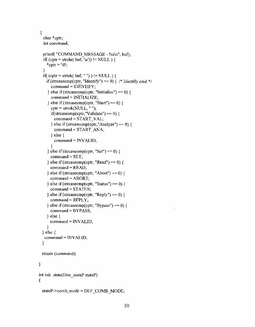
char *cptr; int command;
printf( "COMMAND-MESSAGE - %s\n", buf); if( (cptr = strchr( buf, 'h')) != NULL ) {
*cptr = '\Of; 3 if( (cptr = strtok( buf, 'I ") ) != NULL ) {
if (strcasecmp(cptr, "Identify") == 0) { /* Identify cmd */ command = IDENTIFY;
} else if (strcasecmp(cptr, "Initialize") = 0) { command = INITIALIZE;
1 else if (strcasecmp(cptr, "Start") = 0) { cptr = strtok(NULL, "); if(strcasecmp(cptr,"Validate") == 0) {
} else if (strcasecmp(cptr,"Analyze") = 0) {
3 else {
1
command = START-VAL;
command = START-ANA;
command = INVALID;
} else if (strcasecmp(cptr, "Set") --- 0) {
} else if (strcasecmp(cptr, "Read") = 0) {
} else if (strcasecmp(cptr, "Abort") == 0) {
} else if (strcasecmp(cptr, "Status") == 0) {
} else if (strcasecmp(cptr, "Reply") = 0) {
} else if (strcasecmp(cptr, "Bypass") == 0) {
3 else {
3 } else {
1
command = SET;
command = READ;
command = ABORT;
command = STATUS;
command = REPLY;
command = BYPASS;
command = INVALID;
command = INVALID;
return (command);
int init-state(Dim-stateP stateP) {
stateP->comb-mode = DEF-COMB-MODE;
50

sprintf( stateP->batchgath, DEFBATCH-PATH); sprintf( stateP->samp-type, DEF-SAW-TYPE); sprintf( stateP->samp-id, DEF-SAW-ID); spring( stateP->datafile, DEF-DATAFILE); stateP->inj-voi = DEF-INJ-VOL; stateP->sap amt = DEF-SAW-AMT;
sprintf(stateP->calib-set, DEF-CALIB-SET); sprintfii stateP->surr-set, DEF-CALIB-SET); stateP->qa-scale-flag = DEF-QA-SCALE; stateP->qa-d-flag = DEF-QA-RT; stateP->qa-sur-flag = DEF-QA-SUR; stateP->qa-cal-flag = DEF-QA-CAI.,; return( 0);
stateP->sum-kover = DEF-SUR-RECOVER;
}
int print-state(Dim-stateP stateP) {
switch(stateP->comb-mode) { case COMB-MIN: fprintf(stderr,"Results combination mode: Minimum, \n"); break;
fprintf(stderr,"Results combination mode: Maximum. \n"); break;
fprintf(stderr,"Resuits combination mode: Average. b"); break;
fprintf(stderr,"Results combination mode: Fusion. \n"); break;
fprintf(stderr,l'Results combination mode: PCR Raw. \n"); break;
fprintf(stderr,"Results combination mode: PCR Peak. h"); break;
fprintf(stderr,"Results combination mode: MLR Raw. \n"); break;
fprintf(stderr,"Results combination mode: MLR Peak. \n"); break;
case LRP: fprintf(stderr,"Results combination mode: LR Peak. \n"); break;
fprintf(stderr,"Results combination mode: Neural Network Peak. h");
case COMB-MAX:
case COMB-AVG:
case COMB-FUS:
case PCRR:
case PCRP:
case MLRR:
case MLRP:
case NNP:
51

break;
fprintf(stderr,"Results combination mode: SLE Raw. \n"); break;
default: fprintf(stderr,YJnknown combination mode - error! \n"); return(- 1);
case SLER:
1 fprintf(stderr,"Batch directory path name: %s \n",stateP->batchqath); fprintf(stderr,"Sample type: %s \n",stateP->samp-type); fprintf( stderr,"Sample ID: %s \n",stateP->samp-id); fprintf(stderr,"Datafile name: %s \n",stateP->datafile); fprintf( stderr,"Injection volume: %f uL.\n", stateP->inj-vol); fprintf( stderr,"Sample amount: %f mg.\n", stateP-%amp - amt); fprintf(stderr,"Surrogate amount: %f ng.\n", stateP->surr-amt); fprintf(stderr,"Surrogate recovery: %f percent.\n", stateP->surr-recover); fprintf(stderr,"Calibration set prefix: %s\n",stateP->calib-set); fprintf(stderr,"Surrogate set prefix: %s\n",stateP->sumpset); fprintf(stderr,"QA off-scale flag: %d\n", stateP->qa-scale-flag); fprintf(stderr,"QA retention time flag: %d\n", stateP->qa-rt-flag); fprintf(stderr,"QA surrogate check flag: %d\n", stateP->qa-sur-flag); fprintf(stderr,"QA calibration check flag: %d\n", stateP->qa-cal-flag); return( 0);
1
int set-state(Dim-stateP stateP, char *paramcptr, char 'valcptr)
int flag=O; int ret, rtn-code; float vol; float amt; static char file-name[LBUFF-SIZE]; char *tcptr; char cmdstring[LBUFF-SIZE]; FILE * fp;
Cmd-msg-buf tmsgbuf; /* message send structure */ Cmd-msg-bufP tmsgp; int msgsz, msgflg; long msgtyp;
extern int slmstate; extern int tmsqid;
tmsgp = &tmsgbuf;
tmsgp->mtype = 1 ; msgflg = 0;
52
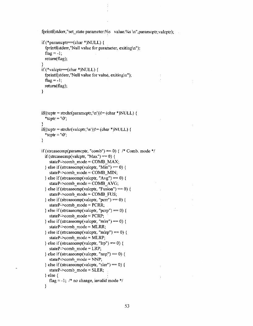
fprintf(stderr,"set-state parameter:%s value:%s \n",paramcptr,valcptr);
if (*paramcptr====(char *)NULL) { fprintf(stderr,"Null value for parameter, exitingh"); flag = -1; return(flag);
1 if (*valcph==(char *)NULL) {
fprintf(stderr,"Null value for value, exiting\n"); flag = -1; return(flag);
1
if((tcptr = strchr(paramcptr,lh'))!= (char *)NULL) { *tcptr = ?\Of;
1
1
if((tcptr = strchr(valcptr,'\n'))!= (char *)NULL) { *tcptr = I\@;
if (strcasecmp(paramcptr, "comb") = 0) { /* Comb. mode */ if (strcasecmp(valcptr, "Max") 0) {
stateP->comb-mode = COMB-MAX; 1 else if (strcasecmp(valcptr, "Min") = 0) {
stateP->comb-mode = COMB-MIN; 1 else if (strcasecmp(valcptr, "Avg") = 0) {
stateP->comb-mode = COMB-AVG, 1 else if (strcasecmp(valcptr, "Fusion") == 0) {
stateP->comb-mode = COMB-FUS; } else if (strcasecmp(valcptr, "pcrr") == 0) {
stateP->comb-mode = PCRR; 1 else if (strcasecmp(valcptr, "pcrp") = 0) {
stateP->comb-mode = PCRP; 1 else if (strcasecmp(valcptr, "mlrr") == 0) {
stateP->comb-mode = MLRR, 1 else if (strcasecmp(valcptr, "mlrp") = 0) {
stateP->comb-mode = MLRP; ] else if (strcasecmp(valcptr, "lrp") == 0) {
stateP->comb-mode = LRP; 1 else if (strcasecmp(valcptr, "nnp") == 0) {
stateP->comb-mode = NNP; ] else if (strcasecmp(valcptr, "sler") = 0) {
stateP->comb-mode = SLER; ) else {
flag = - 1; /* no change, invalid mode */ 1
53

slmstate = IDLE; ) else if(strcasecmp(paramcptr, "batchjath") == 0) {
sprintf( stateP->batchgath, valcptr); if(strcmp(stateP->batchgath, "\O")!=O) { /* batch path has been set */
/* code to run matlab function follows */
sprintf(cmdstring,"code = dim-set-batch('%s')",stateP->batchgath); fprintf(stderr,"Matlab command string:%sh",cmdstring); strncpy(tmsgp->command, cmdstring, LBUFF-SIZE-2);
msgsz = strlen(cmdstring) -t- 1;
/* */
/* */ /* send message to queue *I
rtn-code = msgsnd(tmsqid, tmsgp, msgsz, msgflg); if (rtn-code = -1) {
perror("msgop: msgsnd failed"); 1
} else { flag = -1; fprintf(stderr,"In set batch path: null path argumenth");
1
slmstate = SET-BATCH;
if ((strcasecmpfvalcptr, "standard") == 0) 11 (strcasecmp(valcptr, "unknown") = 0) 1 1 (strcasecmp(valcptr, "control") = 0) 1 1 (strcasecmp(valcptr, "blank") == 0)) { sprintf(stateP->samp--type, valcptr);
flag = -1;
1 else if(strcasecmp(paramcptr, " AIA-samp-type") = 0) {
} else {
1
slmstate = IDLE;
sprintf(stateP->samp-id, valcptr); } else if(strcasecmp(paramcptr, "AIA-sarnp-id") == 0) {
slmstate = IDLE; } else if(strcasecmp(paramcptr, "datafile-name") = 0) {
/* check to see if batchgath and samp-id are set */ if (strcmp(stateP->batchjath, DEFBATCH-PATH) &&
strcmp(stateP->samp-id, DEF-SAMP ID) && !(stateP->samp-amt == DEF-SAMP-~MT)) {
54

sprintf(stateP->datafile, valcptr);
if((fp=fopen(valcptr, "rtl))== (FILE *)NULL) { /* check to see file exists*/
flag = -1; fprintf(stderr,"could not open %s for reading.\n",valcptr);
fclose(fp); } else {
I* create directory */ I* check to see if directory/file exists */
spring( file_name,"%s/0/oss/%s .d", stateP->batchgath, stateP->samp-type, stateP-%amp - id);
if((fp=fopen(file-name, Y))!= (FILE *)NULL) { fprintf(stderr,"%s already exists, no copy, using existing file\n",file-name); fclose(fp); flag= 1; ret = 0;
sprintf(cmdstring,"mkdir %s/%ss/%s.d",
ret = system(cmdstring);
} else {
stateP->batchgath, stateP->samp-type, stateP->samp - id);
1
if(ret != 0) { flag = -1;
1 else { if(flag != 1 ) { sprintf(cmdstring,"chmod 2770 %s/%ss/%s.d",
if(system(cmdstring) != 0) {
} else { /* chmod successful, copy the file */
/* mkdir successful, copy the file */
stateP->batch_path, stateP->samp-type, stareP->samp - id);
flag = -1;
/* copy the file */ sprintf(file_name,"%s/%ss/%s.d/%s.cdf',
stateP->batchgath, stateP->samp-type, stateP->samp-id, stateP->samp-id);
sprintf(cmdstring,"cp %s %st1,valcptr, file-name);
if(system(cmdstring) != 0) {
} else { flag = -1;
/* copy successful, poke ALA values *I amt = state€'->samp-amt; if(aiagoke(fi1e-name, stateP->samp-type, amt) == 0) {
1 else { fprintf(stderr,"poke AIA header values\n");
flag = -1; fprintf(stderr,"could not poke AIA header values in % s h "
55

,file-name); 1
1 1
1 flag = 0; /* work around for warning causing an Error state in TSC*/
1 1
} else { flag = -1; fprintf(stderr,"Batch path, sample ID, or sample amt not set.\n");
1
slmstate = IDLE;
if(sscanf(valcptr,"%f', &vol) > 0) {
} else {
} else if(strcasecmp(paramcptr, " AIA-inj-vol") -- 0) {
stateP->inj - vol = vol;
fprintf(stderr,"Could not convert %s to injection volumn\n",valcptr); flag = - 1 ; I* not proper format for numeric conversion */
1 slmstate = IDLE;
} else if(strcasecmp(paramcptr, "AIA-samp-amt") = 0) { if((ret=sscanf(valcptr,"%f %s", &amt, crndstring)) > 0) {
/* check for units *I if(ret = 2) { I* units present *I
stateP->samp-amt = amt;
amt = amt * 1000.0; stateP->samp-amt = amt;
amt = amt * 1000000.0; stateP->samp-arnt = amt;
fprintf(stderr,"Could not convert %s to MKS units.\n",cmdstring); flag = -1; I* undefined units */
if(strcasecmp(cmdstring,"mg") = 0) {
}else if (strcasecmp(cmdstring,"g") = 0) {
)else if (strcasecmp(cmdstrinp,"kg") = 0) {
)else {
1
stateP->samp-amt = amt * 1000.0; } else { /* assume units in g */
1 } else {
fprintf(stderr,"Could not convert '%OS to sample amount.\n",valcptr); flag = - 1; I* not proper format for numeric conversion *I
1 slmstate = IDLE;
if((ret=sscanf(valcptr,"%f ?'OS", &amt, cmdstring)) > 0) { } else if(strcasecmp(paramcptr, "sum-arnt") == 0) {
I* check for units *I
56
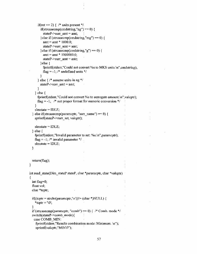
if(ret == 2) { /* units present */
stateP->sum-amt = amt;
amt = amt * 1000.0; stateP->surr_amt = amt;
amt = amt * 1000000.0; stateP->sun-amt = amt;
fprintf(stderr,"Could not convert %s to MKS units.\n",cmdstring); flag = - 1 ; /* undefined units */
if(strcasecmp(cmdstring,"ng") == 0) {
)else if (strcasecmp(cmdstring,"mg") = 0) {
)else if (strcasecmp(cmdstring7"g") == 0) {
}else {
1 else { /* assume units in ng */ stateP->surr-amt = amt;
1 ] else {
fprintf(stderr,"Could not convert %s to surrogate amount.\n",valcptr); flag = - 1 ; /* not proper format for numeric conversion */
1 slmstate = IDLE;
sprintf(stateP->sum-set, valcptr); } else if(strcasecmp(paramcptr, "sum-name") = 0) {
slmstate = IDLE;
fprintf(stderr,"Invalid parameter to set: %s.\n",paramcptr); flag = -1; /* invalid parameter */ slmstate = IDLE;
} else {
I
return( flag); 1
int read-state(Dim-stateP stateP, char *paramcptr, char *valcptr)
int flag=O; float vol; char *tcptr;
if((tcptr = strchr(paramcptr,?n'))!= (char *)NULL) {
1 if (strcasecmp(paramcptr, "comb") == 0) { /* Comb. mode */ switch( stateP->comb-mode) {
"tcptr = '\Of;
caseCOMB-MIN: fprintf(stderr,"Results combination mode: Minimum. h"); spr intf(va1c ptr, "MINlO " ) ;
57

break;
fprintf(stderr,''Results combination mode: Maximum. \n"); sprintf(valcptr,"MAX\O"); break;
fprintf(stderr,"Results combination mode: Average. \n"); sprintf(valcptr," AVG\O"); break;
fprintf(stderr,"Results combination mode: Fusion. h"); sprintf(valcptr,"FUSIONO"); break;
default: fprintf(stderr,"Unknown combination mode I error! \n"); return(-1);
case COMB-MAX:
case COMB-AVG:
case COMB-FUS:
1 ] else if(strcasecmp(paramcptr, "Batchgath") = 0) {
fprintf( stderr,"Batchgath:%s\n",stateP->batch_path); sprintf(valcptr,"%s\O",stateP->batchgath);
} else if(strcasecmp(paramcptr, " AIA-samp-type") = 0) { fprintf(stderr,"AIA-sample-type:%s\n",stateP->samp ._ type); sprintf(valcptr, "%s\O",stateP->samp-type) ;
fprintf( stderr,"AIA-sample-id:%s\n",stateP->samp-id); sprintf(valcptr, "%s\O",stateP->samp-id);
} else if(strcasecmp(paramcptr, "datafile-name") == 0) { fprintf( stderr,"Datafile-name: %s\n",stateP->datafi le); sprintf(valcptr,"%s\O",stateP-dataf file);
} else if(strcasecmp(paramcptr, " AIA-in.-vol") = 0) { fprintf( stderr,"AIA-inj-vol:%f\n",stateP->inj-vol); sprintf(valcptr,"%fO",stateP->inj-vol);
fprintf(stderr,"AIA-samp-amt:%f\n",stateP-%amp - amt); sprintf(valcptr,"%fO'17stateP->sarnp-amt);
fprintf(stderr,"Surrogate amount:%f ng\n",stateP->sum - amt); sprintf(valcptr,l'%fO'',stateP->surr - amt);
fprintf(stderr,"Surogate recovery:%f percent\n",stateP->surr-recover); sprintf(valcptr,"%fO'17stateP->surr-amt);
fprintf(stderr,"Calibration file prefix:%s\n",stateP->calib-set); sprintf(valcptr,"%s\O",stateP-Xalib-set);
fprintf(stderr,"Surrogate name:%s\n",stateP->surr-set); sprintf(valcptr,"%s\O ",stateP->surr-set);
flag = - 1; /* invalid parameter */
} else if(strcasecmp(paramcptr, " AIA-samp-id") == 0) {
} else if(strcasecrnp(paramcptr, "AIA-samp-amt") == 0) {
] else if(strcasecmp(paramcptr, "surr-amt") == 0) {
} else if(strcasecmp(paramcptr, ''sun-recover") == 0) {
} else if(strcasecmp(paramcptr, "calqrefix") = 0) {
} else if(strcasecmp(paramcptr, "sum-name") -- 0) {
} else {
58

1 return(flag);
1
void dim-en-code(int err-no, char *buffer) {
switch(en-no) { case INIT-ERR:
break; case BAD-ARG:
break; case MATLAB-ENGINE-OPEN:
break; case BATCH-DIR-UNSET:
break; case SAMPLE-ID-UNSET:
break; case DATAFILE-UNSET:
break; default:
strcpy( buffer, "Initialization failed");
strcpy(buffer,"Bad Argument for command");
strcpy( buffer,"Couid not open MATLAB engine");
strcpy(buffer,"Pathname to batch processing directory not set");
strcpy(buffer,"Sample ID not set");
strcpy(buffer,"Filename of raw AIA file not set");
if (en-no < 0) { sprintf(buffer,"%s %s",decipher-en-codes(err-no, 1 ),
de~ipher-err-codes(err-no~2)); } else {
1 strcpy(buffer,"No error text");
break;
1 1
/* check to see if necessary parameters have been set */
int check-stateCDim-stateP stateP) {
int flag;
flag = 0;
if (! strcmp(stateP->batchjath, DEFBATCH-PATH)) {
1 else if (!strcmp( stater)->samp-id, DEF-SAMP-ID)) { flag = BATCH-DJR-UNSET;
flag = SAMPLE-ID-UNSET;
59

} else if (! strcmp( stateP->datafile, DEF-DATAFILE)) {
} else if (stateP->samp-amt == DEF-SAMP-AMT) {
} else if (stateP->surr-amt == DEF-SUR-AMT) {
} else if (stateP->surr-set = DEF-SUR-SET) {
flag = DATAFILE-UNSET;
flag = SAMPLE-AMT-UNSET;
flag = SURROGATE-AMT-UNSET
flag = SURROGATENAME-INSET; 1
return( flag); 1
/* validate gc *I
int validate(Dim-stateP stateP)
{
char cmdstring[LBUFF-SIZE+ 11; int rtn, rtn-code; float recovery; Rtn-msg-buf rmsgbuf; /* message send structure *I Rtn-msg-bufP rmsgp;
Cmd-msg-buf tmsgbuc I* message send structure *I Cmd-msg-bufP tmsgp; int msgsz, msgflg; extern int tmsqid, rmsqid; extern int slmstate;
long msgtyp;
tmsgp = &tmsgbuf; rmsgp = &rmsgbuf;
tmsgp->mtype = 1 ; msgflg = 0;
I* get calibration file prefix *I sprintf(cmdstring,"[result, code] = calgrefix;"); fprintf( stderr,"%s\n", cmdstring);
msgsz = strlen(cmdstring) + 1; if (msgsz > LBUFF-SIZE) msgsz = LBUFF-SIZE; strncpy(tmsgp->command, cmdstring, msgsz);
I* *I
I" *I 1" send message to queue *I
rtn-code = msgsnd(tmsqid, tmsgp, msgsz, msgflg); if (rtn-code == - 1) {
60

perror("msgop: msgsnd failed"); slmstate = IDLE; return( rtn-code);
1
I* wait for return message *I rnsgtyp = 0; if(msgrcv(rmsqid, rmsgp, MSG-SIZE, msgtyp, O)>=O) {
printf("\nresponse from peer received\n"); rtn = rmsgp->code; if (rtn == 0) {
fprintf( stderr, "Matlab call successful\n"); strncpy(stateP->calib-set, rmsgp>result, LBUFF - SIZE-2);
slmstate = IDLE; fprintf( stderr, "Matlab call error\n"); return(rtn);
} else {
1 1
I* preprocess the raw file "1 sprintf(cmdstring,"code = preprocessgc('%s/%ss/%s.d/%s.cdf, - l)",
fprintf(stderr,"%s\n", cmdstring); stateP->batchgath,stateP->samp-type,stateP->samp - id,stateP->amp - id);
msgsz = strlen(cmdstring) + 1; if (msgsz > LBUFF-SIZE) msgsz = LBUFF-SIZE; stmcpy(tmsgp->command, cmdstring, msgsz);
I* *I I* send message to queue /* *I
rtn-code = msgsnd(tmsqid, tmsgp, msgsz, msgflg); if (rtn - code == -1 ) {
perror("msgop: msgsnd failed"); slmstate = IDLE; return(rtn_code);
1
I* send progress message *I TKProgress( 90, "Preprocessing chromatogram.", -1);
I* wait for return message *I msgtyp = 0; if(msgrcv(rmsqid, rmsgp, MSG-SIZE, msgtyp, O)>=O) {
printf("\nresponse from peer received\n"); rtn = rmsgp->code; if (rtn == 0) {
61

fprintf( stderr, "Matlab call successful\n");
slmstate = IDLE; fprintf(stderr, "Matlab call error\n"); ret um(rtn) ;
} else {
1 I
/* qa check for off scale signal */
qa-off - scale('%s/%ss','%s/software_code/mat~a~,'~~s/st~dards','~~s/%ss/%s.d/~~s.cdf , I)", - sprintf(cmdstring,"[code, minqts, maxgts] -
stateP->batchgath,stateP->samp-type, stateP->batchgath,stateP->batchgath, stateP->batchgath,stateP->samp-type,state,P->samp - id,stateP->samp - id);
fprintf(stderr,"%s\n", cmdstring); msgsz = strlen(cmdstring) + 1 ;
stmcpy(tmsgp->command, cmdstring, msgsz); if(msgsz > LBUFF-SIZE) msgsz = LBUFF-SIZE;
/* */ /* send message to queue /* */
*/
rtn-code = msgsnd(tmsqid, tmsgp, msgsz, msgflg); if (rtn-code == -1) {
perror("msgop: msgsnd failed"); slmstate = IDLE; retum(rtn-code);
l
/* send progress message */ TKProgress( 60, "QA check for off scale signal.", - 1);
/* wait for retum message */ msgtyp = 0; if(msgrcv(rmsqid, rmsgp, MSG-SIZE, msgtyp, O)>=O) {
printf("\nresponse from peer received\n"); rtn = nnsgp->code; if (rtn = 0) {
fprintf(stderr, "Matlab call successfulh''); stateP->qa-scale-flag = 1 ;
slmstate = IDLE; fprintf(stderr, "Matlab call errorh"); stateP->qa-scale-flag = - 1; return( rtn);
} else {
1 1
/* qa check for retention time markers */
62

- sprintfii cmdstring," [code, distance] - qa-retention - m a r k ( ' % s l % s s ' , ' % s / s o f h v a r e _ c o d e l m a t l a b ' , , 1>",
stateP->batchqath,stateP-%amp type, stateP->batchgath,st ateP->batch>ath, stateP->batchgath,stateP->samp-~e,statp-id,stateP->samp - id);
fprintf(stderr,"%s\nI', cmdstring); msgsz = strlen(cmdstring) + 1; if (msgsz > LBUFF-SIZE) msgsz = LBUFF-SIZE; strncpy(tmsgp->command, cmdstring, msgsz);
I" */ /* send message to queue I* *I
*/
rtn_code = msgsnd(tmsqid, tmsgp, msgsz, msgflg); if (rtn-code = - 1) {
perror("msgop: msgsnd failed"); slmstate = IDLE; return( rtn-code);
1
1" send progress message "I TKProgress( 30, "QA check for retention time markers.", -1);
/* wait for return message */ msgtyp = 0; if(msgrcv(rmsqid, rmsgp, MSG-SIZE, msgtyp, O)>=O) {
printf("\nresponse from peer receivedh"); rtn = rmsgp->code; if (rtn = 0) {
fprintf(stderr, "Retention time qa check passed\n"); stateP->qa-rt-flag = 1 ;
slmstate = IDLE; fprintf(stderr, "Retention time qa check failed\n"); stateP->qa-rt-flag = - 1 ; return( rtn);
} else {
I 1
/* determine surrogate recovery */ sprintf(cmdstring,"[code, result, obs, recovery] = dim-test-surrogate('%s', %g,
'%s/%ss/O/Ds.d/%s.cdf , - l)", stateP->surr-set, stateP->surr-amt, stateP->batchjath,stateP->smp-type, stateP->samp-id, stateP->samp-id);
/* sprintf(cmdstring,"[result, code] = runSUR('tcmx','%s/%ss/%s.d/%s.cdf , - 1 )",
stateP->batch~ath,stateP->samp_type,stateP->samp_id,stateP->samp I id); */
fprintf( stderr,"%s\n",. cmdstring);
63

msgsz = strlen(cmdstring) -I- 1; if (msgsz > LBUFF-SIZE) msgsz = LBUFF-SIZE; strncpy(tmsgp->command,' cmdstring, msgsz);
/* */
/* *I /* send message to queue */
rtii-code = msgsnd(tmsqid, tmsgp, msgsz, msgflg); if (m-code == -1) {
perror("msgop: msgsnd failed"); slmstate = IDLE; return(rtn-code);
1
/* check to see if sample type is control */ if(strcasecmp(stateP->samp-type,"control") = 0) {
TKProgress( 15, "QA check for control sample type.", - 1); /* wait for return message */
msgtyp = 0; if(msgrcv(msqid, rmsgp, MSG-SIZE, msgtyp, O)>=O) {
printf("\nresponse from peer received\n"); sscan f(rmsgp->result,"%g",&recovery); stateP->surr-recover = recovery; rtn = rmsgp->code; if (rtn == 0) {
fprintf( stderr, "Matlab call successful\n"); stateP->qa-sur-flag = 1 ;
slmstate = IDLE; fprintf(stderr, "Matlab call errorh"); stateP->qa-sur-flag = - 1 ; return(rtn);
} else {
1 1
/* analyze the sample */ sprintf(cmdstring,"[result, code] = dim-analyze('%s','%s', %d)",
stateP-%amp-type,stateP->samp-id, stateP->comb-mode); fprintf( stderr,"%s\n", cmdstring); strncpy(tmsgp->command, cmdstring, LBUFF-SIZE-2); msgsz = strlen(cmdstring) + 1;
/* */ /* send message to queue /* */
*/
rtn = msgsnd(tmsqid, tmsgp, msgsz, rnsgflg); if (rtn == -1) {
perror("msgop: msgsnd failed"); slmstate = IDLE; return(rtn-code);
}
64

I* wait for return message *I msgtyp = 0; if(msgrcv(rmsqid, rmsgp, MSG-SIZE, msgtyp, O)>=O) {
printf("\nresponse from peer received\n"); rtn = rmsgp->code; if (rtn I== 0 ) {
1 else { fprintf(stderr, "Matlab call successfulh");
slmstate = IDLE; fprintf(stderr, "Matlab call error\n"); return(rtn);
1 1
TKProgress( 30, "QA check for calibration standard.", - 1);
sprintf(cmdstring,"[code, known-conc, percent-em] = qa-cal-check(result,
stateP->batchgath,stateP->sarnp-type, stateP->batchqath,stateP->batchqath, stateP->batchgath,stateP->samp_type,stateP->samp-id,s~teP->s~p - id); fprintf(stdem,"%s\nr', cmdstring); strncpy(tmsgp->command, cmdstring, LBUFF - SIZE-2); msgsz = strlen(cmdstring) + 1 ;
I* perform calibration QA check *I
'%s/%ss','%s/sofhvare - code/matlab','%s/standards','%s/%ss/%s.d/%s.cdf , 1 )",
I* *I I* send message to queue */ I* *I
rtn = msgsnd(tmsqid, tmsgp, msgsz, msgflg); if (rtn = -1) {
perror("msgop: msgsnd failed"); slmstate = IDLE; return( rtn-code);
1 f else {
I* send progress message *I TKProgress( 15, "QA check for surrogate recovery.", - 1);
stateP->qa-cal-flag = 0; I
return(rtn); I
1" analyze gc *I
int analyze(Dim-stateP statel?) {
65

char cmdstring[LBUFF-SIZE+ 13; extern Engine *ep; extern char *mat-output; Matrix *matrix-out; double *code; int rtn;
Cmd-msg-buf tmsgbuf; /* message send structure *I Cmd-msg-bufP tmsgp; int msgsz, msgflg; extern int tmsqid, rmsqid; extern int slmstate;
long nWYp;
tmsgp = &tmsgbuf; tmsgp->mtype = 1; msgflg = 0;
if( strcasecmp(stateP->samp-type, "unknown") == 0) { I* analyze the sample */
sprintf(cmdstring,"[result, code] = dim-analyze('%s','%s', %d)", stateP-%amp-type,stateP->samp-id, stateP->comb-mode);
fprintf( stderr,"%s\n", cmdstring); stmcpy(tmsgp->command, cmdstring, LBUFF-SIZE-2); msgsz = strlen(crndstring) + 1;
I* send progress message */ TKProgress( 90, "Analyzing chromatogram.", - 1);
/* *I
/* */ /* send message to queue */
rtn = msgsnd(tmsqid, tmsgp, msgsz, msgflg); if (rtn == -1) {
1 perror("msgop: msgsnd failed");
} else { /* not an "unknown" sample type */
slmstate = IDLE; fprintf(stderr, "Can't analze %s sampe type\n", stateP->samp-type); rtn = -850;
return( rtn); 1
66

err-c0de.C
11 ERRC0DES.C I* Written by: B. B Spencer I* Version: OS-20-96 "1 11 Provides description of error codes for GC DIM. #include <stdio.h> #include <stdlib.h> #include <string.h>
*I
/*----- This function deciphers the error codes. -----*I extern "C" char *decipheren--codes(int numerr,int iopt) /* Written by: B. B Spencer I* Version: 08-20-96 "I 11 numerr is the error code to be deciphered 11 iopt takes on only 3 values: I/ 11 11
typedef struct errcodes { char *funcname; int errnum; char *verbose;
*I
1 means get the function name where the error occured 2 means describe the error 9 means list all the error codes and their definitions
{
) Errcodes;
ErrCodes described[] = {
{ "response-raw.m", - 10, %Opening of file response-raw.parm failed, Possibleh" "\tcauses are: file was not created or the parmsubdirh" "\tvariable does not contain a subdirectory pointing to\n" "\tthe file."),
{"response-raw.m", -1 1 , %The specified raw data file could not be opened."),
{ "select-data.mIl, -20, "\tNo raw data exists when a request to select data was\n" "\tissued."),
( "select-data.m", -2 1, "\tOpening of file select - data.parrn failed. Possible\n" "\tcauses are: file was not created or the parmsubdir\n" "\tvariable does not contain a subdirectory pointing toh" "\&e file."),
{ "select-data.m", -22, "\tThe contents of select-data-parm are inconsistent, theh"
67
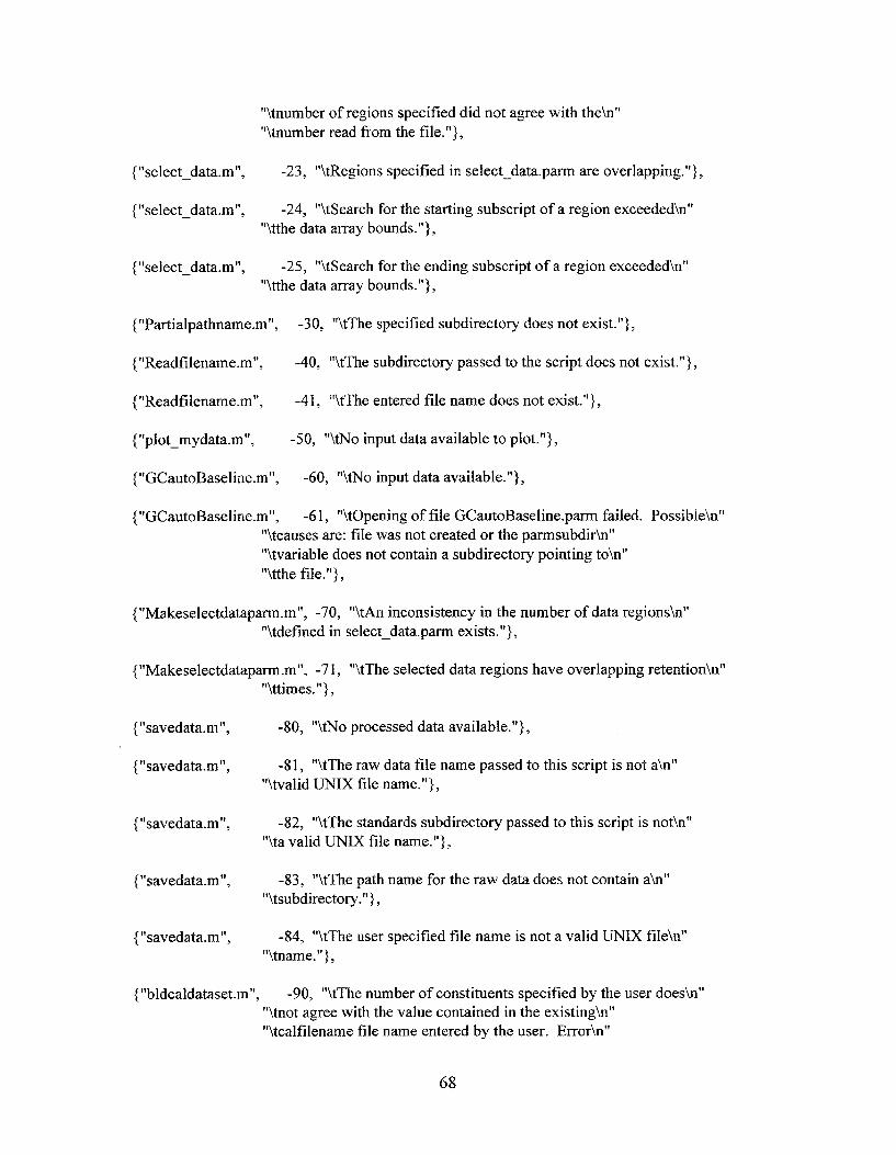
"\tnumber of regions specified did not agree with the\n" "\tnumber read from the file."},
{ "select-data.mIl,
{ "select-data.m",
-23, '?Regions specified in select-data.parm are overlapping."} ,
-24, "\tSearch for the starting subscript of a region exceeded\n" "\tthe data array bounds."} ,
{ "select-data.m", -25, "\tSearch for the ending subscript of a region exceeded\n" "\tthe data array bounds."},
{ "Partialpathname.m",
{ "Readfilename.m",
{"Keadfilename.m",
{ 'lplot-mydata.m",
{ "GCautoBaseline.m",
{ "GCautoBaseline.m",
-30, "\tThe specified subdirectory does not exist."} ,
-40, "\tThe subdirectory passed to the script does not exist."} ,
-4 1, "\tThe entered file name does not exist."},
-50, "\tNo input data available to plot."},
-60, "\tNo input data available."),
-6 1, "\tOpening of file GCautoBaseline.parm failed. Possible\n" "\tcauses are: file was not created or the parmsubdirb" "\tvariable does not contain a subdirectory pointing to\n" "\tthe file."},
{ "Makeselectdatapann.m", -70, 'VAn inconsistency in the number of data regions\n" "\tdefined in select-data.parm exists.") ,
{ "Makeselectdataparm .m", -7 1 , "\tThe selected data regions have overlapping retention\n" "\ttimes.") ,
{ "savedata.m",
{ "savedata.m",
{ 'lsavedata.m",
{ "savedata.m",
{ "savedata.m",
-80, "\tNo processed data available."} ,
-8 1 , "\tThe raw data file name passed to this script is not a\n" "\tvalid UNIX file name."},
-82, "\tThe standards subdirectory passed to this script is not\n" "\ta valid UNIX file name."},
-83, "\tThe path name for the raw data does not contain a b " "\tsubdirectory." } ,
-84, "\tThe user specified file name is not a valid UNIX file\n" "\tname."} ,
{ "bldcaldataset.m", -90, "\tThe number of constituents specified by the user doesb" "\tnot agree with the value contained in the existingh" "\tcalfilename file name entered by the user. Errorh"
68

"\tis probably the result of an attempt to add data toh" "\tcalfilename from a raw data file not appropriate\n" "\Ifor the existing calibration data information or by a\n" "\tchange in the regions specified in select-data.parm fileh" "\tthat changed the total number of data points selectedh" "\tby select-data.m.") ,
{ "bldcaldataset.m", -91, "\tThe number of points determined for the current data\n"
("timeshifLm",
( "timeshift.m",
{"timeshift.m",
{ "timeshift.m",
"\tarray does not agree with the value specified in the\n" "\texisting calfilename file entered by the user.") ,
- 100, "\tNo input data avaifable when a request to align the\n" "\tinput data was made."} ,
- 10 1 , "\tOpening of file retentionmarkers.dat failed. Possibleh" "\tcauses are: file was not created or the datasubdir\n" "\tvariable does not contain a subdirectory pointing to\n" "\tthe file.") ,
- 102, '%Data inconsistency in file retentionmarkers.dat was\n" "\tdetected. The number of markers specified in the fileh" "\tdoes not agree with the actual number contained in\n" "\tthe file."),
- 103, "\tThe search for the first retention time marker failed\n" "\tafter the data was aligned to the mean value of theh" "\tfirst retention time marker in the calibration data set."),
{ "response-set.m", - 1 10, '%The file defined by calfilename could not be\n" "\tlocated. " } ,
{ "response-set.m", - 1 1 1, "\tThe parameter file response-set.parm could not be\n" '%located. Either the file was not created or theh" "\tvariable parmsubdir does not point to the correct\n" "\tsubdirectory."),
{ "response-set.m", - 1 12, "\tAn inconsistency between the defined data processingh" "\toptions and those specified in file calfilename\n" %was detected. This will cause a fatal error if theh" "\tnumber of data processing options are different."},
{ "response-set.m", - 1 13, "\tA \"A1' character was not found as the first characterh" "\tin the file name for the data file being read. This\n" "\terror probably results from problems reported by\n" "\tError Code -1 12."),
{"response-set.mIl,
{ "response-set.m",
-1 14, "\tThe specified data file could not be located."),
-1 15, %An inconsistency between the number of points in the\n"
69

"\tdata file specified in file calfilename and actually\n" "\tread has been detected."},
{ "response-set.mIl, - 1 16, "\tThe UNIX command \"basename\" from withinb" "\tresponse-set.m failed while attempting to obtain the\n" "\tfile name for a standard."},
{ "pcamodelbld.m", - 120, "\tInvalid preprocessing option. Notify authors whenh" "\tthis error occurs."},
{ "pcamodelbld.m", - 12 1, "\tGreater than 10% of the response matrix has zero\n" "\tvariance. Suggest using an alternated data processing\n" "\toption."},
{ "pcamodelbld.m", -122, "\tA constituent in the data set is invariant. CanYt model\n" "\tthis data."},
{ "pcamodelbld.m",
{ " pcamodelbld.m",
- 123, "\tThe regression equations are numerically unstable."},
-124, "\tThe task of building a new PCR calibration modelh"
{ "integrate.m",
{ "integrate.m",
{ "integrate.m",
{ "integrate.m",
{ "decimation.m",
{ "decimation.m",
{ "decimation.ni",
{ "psdscript.m",
{ "ana1bypcr.m 'I,
{ " analbypcr . m 'I,
"\twas not executed; the user elected to retain anh" "\texisting calibration model file based upon the enteredb" "\tcalibration information data file."},
- 130, "\tNo input data available."} ,
- 13 1, "\tCan not locate the parameter file integratiomparm in\n" "\tthe specified parameter subdirectory."},
-132, "\tSearch for the start of the integration region exceededh" "\tthe data array bounds."},
- 133, "\tWorking index exceeded the data array bounds. \n" "\tSuggest the number of integration intervals be\n" "\tdecreased."},
-140, "\tNo input data available."},
-141, "\tCan not locate the parameter file decimation.parm in\n" "\tthe specified parameter subdirectory."),
- 142, "\tDecimation order is outside the allowed range."},
- 150, "\tNo input data available to process."},
- 160, "\tCalibration information file could not be opened."},
- 16 1, "\tCalibration model file could not be opened."},
70

{ "analbypcr.m",
{ "analbypcr.m",
{ "analbypcr.m",
{ "ana1bypcr.m ",
{ "analbypcr.m",
{ "analbypcr.m",
{ "analbypcr.m",
- 162, "\tCalibration model file does not contain a PCR model."} ,
- 163, "\tNumber of constituents in the calibration informationh" "\tfile and the calibration model file do not agree."),
- 164, "\tDisagreement between the number of points for the\n" "\tprocessed data listed in the calibration infonnation\n" "\tfile and the calibration model file."),
- 165, "\tSample data array size is not consistent with the array\n" "\tsizes used in the calibration model."},
- 166, "\tCalibration information file name CANNOT end withh" "\tthe suffix \lv.fhct\ll.l'),
- 1 67, "\tThe concentration normalized peak-area file could not\n" "\tbe located."),
- 168, "\tThe PCR model filename could not be extracted from theh" "\tcomplete pathname of the PCR model file."),
{ "BaseSetData.m",
{ "BaseSetData.m",
{ "BaseSetData.m",
{ "polybasefit.m",
{ "polybasefit.m",
- 170, "\tNo input data available."},
-1 71, "\tParameter file, BaseSetData.parm, can not be located."),
-172, "\tSearch for a data region exceeded array bounds."),
- 180, "\tNo input data available to process."},
- 18 1 , "\tParameter file polybasefit-m could not be located inh" "\tthe currently defined parameter subdirectory."},
{ "polybasefit.m", - 182, %The parameter file po1ybasefit.m could not be openedh" "\tfor saving of the new parameter values."),
("gen-filegarm.m", - 190, %Model pathname is not a fully qualified pathname,h" "\ti.e., the pathname does not start with the \"A"\n" "\tcharacter . " ) ,
(lqgen-fileqarm.m", -191, %Data pathname is not a fully qualified pathname, i.e.,h" "\tthe pathname does not start with the \''A'' character."},
{"gen-fileqarm.m", - 192, "\tModel pathname is in the system root directory. This\n" "\tlocation is not allowed."),
{"gen-filegarm.m", -193, "\tData pathname is in the system root directory. Thish" "\tlocation is not allowed."),
{ "gen-fileqarm.m", - 194, "\tModel pathname contains only a file name."),
71

("gen-filegarm.m", -19.5, "\tData pathname contains only a file name."} ,
{ "gen-file_parm.m", -196, "\tThe pathname does not agree with the defined\n" "\tsubdirectory structure."},
{ "locretentmark.m", -200, "\tNo input data available when the request to locate\n" "\tretention time markers was made.") ,
{ "locretentmark.m", -20 1 , "\tSearch for the start of the region where the retentionh" "\ttime marker should be located exceeded the array\n" "\tbounds."},
{ "locretentmark.m", -202, "\tSearch for the end of the region where the retentionh" "\ttime marker should be located exceeded the array\n" "\tbounds."},
{ "locretentmark.m", -203, "\tAn inconsistency between the number of markers\n" "\tspecified in file retentionmarkexdat and the cumently\n" "\tspecified number of markers was detected,"},
{ "locretentmark.m", -204, "\tNo raw data available."},
{ "student.m", -2 10, "\tZero degrees of freedom was passed to the function;\n" "\tthis yields an undefined t value."},
{ "student.m", -2 1 I , "\tProbability level greater than 0.999 is not allowed;\n" "\terrors in the calculation o f t become significant ath" "\tsmall degrees of freedom." j ,
{ "studentm", -212, "\tProbability level of zero was passed to the function."},
{ "openGC.m", -220, "\tSpecified data file could not be opened." j ,
{ %aveAIA .m It7 -230, "\tFilename or data arrays passed to the function arch" "\tnull arrays."},
( "saveAIA.m", -23 1, "\tThe root filename passed to the function is a not\n" "\tdefined."),
{ "fourierbaseline.m", -240, %No data was passed to the function." j ,
{ "fourierbaseline.m", -24 1, "\tParameter file \"fourierbaseline.parm\" could not be\n" Il\topened.''),
{ "fourierbaseline.ml', -242, %The file \"fourierbaseline.parm\" could not be opened\n" "\tto write the new parameters."},
{"preprocessgc.m", -250, "\tThe UNIX command to obtain the directory name o h "
72

"\tthe data failed."},
{"preprocessgc.m",
{ "preprocessgc.m",
-25 I, "\tThe directory for the sample does not exist."),
-252, *%The file containing the data preprocessing options\n" "\tcould not be opened."),
{ "preprocessgc.m", -253, "\tThe file to save the preprocessing options could not\n" "\tbe opened."),
{ knalbysle.ml',
{ "analbysle.m",
{ "analbysle.m",
{ llanalbysle.m",
{ "analbysle.m",
{ "analb ys le, m " ,
{"fixname,m",
{ "fixname.m",
("fixname.m",
{ "runsleF .m ' I ,
-260, "\tThe UNIX command to obtain the directory name o h r ' "\tthe data failed."),
-261, "\tThe UNIX \"Is\" command failed or a calibration data\n" "\tset file does not exist."},
-262, "\tThe specified calibration data set file could not beh" "\topened.") ,
-263, '%More standard files specified than are contained inh" "\tthe calibration data set file.") ,
-264, "\tThe condition number of the matrix for theh" "\tcalibmtion model is infinite; the unknown can not beh" "\tanalyzed using the specified standards." ) ,
-265, "\tThe subdirectory for the specified sample does not\n" "\texist.l'},
-270, "\tThe input filename does not contain the suffix \"CDF\"\n" ''\tor \"cdf\"."),
-27 1, "\tThe input filename contains the \"CDF\" suffix, whichb" "\twas converted to \"cdf\" but the file with the new suffix\n" "\tdoes not exist."),
-272, "\tThe input filename contains the \"cdf\" suffix, which\n" "\twas converted to \"CDF\" but the file with the new\n" "\tsuffix does not exist."),
-280, "\tNo standard files were specified.") ,
{ "savepcrpeaks.m", -290, "\tPeak set data is not available."),
("savepcrpeaks.m", -29 1, "\tFile to save the peak retention times could not be\n" "\topened."} ,
{"set-dimgath.m", -300, "\tAn error occurred while the MATLAB path was being \n" "\tdetennined."),
73

{ "set-dimqath.m",
{ "set-dimqath.m",
-30 1 , "\tDetermination of sample batch pathname failed."} ,
-302, "\tAn error occurred while adding ../software-code/nn\n" "\tto the MATLAB path."},
{ "set-dimgath.m", -303, "\t4n error occurred while adding ../software-codelmatlabh" "\tto the MATLAB path."},
{ "set-dimgath.m", -304, "\tAn error occurred while adding ../software-code/general\n" "\tto the MATLAE3 path."},
{ "mlrmodelbld.m",
{ "mlrmodelbld.m",
-3 10, "\tNo * .peakset files were identified."},
-3 1 1, "\tUNIX command to obtain the file basename from the fullh" "\tpathname failed."} ,
{ "mlrmodelbld.m",
{ "rnlrmodelbld.m",
-3 12, "\tUser did not select a *.peakset file."},
-3 13, "\tUser attempted to build a new calibration model but did\n" "\tnot allow the overwriting of an existing model file."},
{ "rnlrmodelbld.m",
{ "mlrmodelbld.rn",
{ "mlrmodelbld.rn",
{ "rnlrmodelbld.m",
-3 14, "\tOpening the file to save the calibration model failed\n"} ,
-3 15, "\tThe peak time parameter could not be opened\n"),
-3 1 6 , "\tThe user did not select any peaks for the MLR modelh"} ,
-3 17, '%The condition number of the coefficient matrix for t h e h "
{ "analbymlr.m",
{ "analbymlr.m",
{ "analbymlr.mtl,
{ I' analb ym lr I m 'I ,
{ " analbym lr .m ",
{ "analbymlr.m",
{ "analbymlr.m",
"\tnormal equations suggests any MLR models using theh" "\tspecified calibration data set will yield unstable results."},
-320, ''\tNo * .peakset file was identified.\n"} ,
-32 1, "\tUNIX \"basename\" command failed.\n"},
-322, "\tUNIX \"dirname\" command failed.\n" } ,
-323, "\tThe specified directory does not exist.\n"} ,
-324, "\tThe specified MLR calibration file could not be opened.\n"},
-325, "\tThe specified calibration file is not an MLR model.\n"},
-326, "\tThe group file could not be opened.\n"),
{ "qa-retentmark.m", -330, "\tIncorrect number of parameters passed to the\n" "\tfunction."} ,
74


0RNLi"M.-13572
INTERAL DISTRIBUTION
1 .-3. M. A. Hunt 4. J. M. Jansen 5. M. L. Jernigan 6.-10. L. N. Klatt 1 1 . D. W. McDonald 12. D. H. Thompson 13. K. W. Tobin 14. J. R. Younkin 15.-16. Central Research Library 17.-18. Laboratory Records 19. Laboratory Records-Record Copy 20. ORNL Patent Section 2 1 . Y- 12 Technical Library-Document Reference Center
EXTERNAL DISTRIBUTION
22. M. Clark, INEL Site Manager, Idaho National Engineering Laboratory, PO Box 1625 MS- 2220, Idaho Falls, ID 83415.
23. R. M. Hollen, CAA Program Coordinator, Los Alamos National Laboratory, PO Box 1663, MS-J580, Los Alamos, NM 87545.
24-33. K. Humphrey, Program Administrator, Los Alamos National Laboratory, PO Box 1663, MS-J580, Los Alamos, NM 87545.
34. J. Noble-Dial, ORO-DOE, 55 Jefferson, Rm219F, MS-91, Oak Ridge, TN 3783 1.
139

'if ac42 is absent and ac54 is present and ac60 is absent and import is medium then
'if ac42 is absent and ac54 is present and ac60 is absent and import is low then
'if a042 is absent and ac54 is absent and ac60 is present and import is high then
'if a d 2 is absent and ac54 is absent and ac60 is present and import is medium then
'if ac42 is absent and ac54 is absent and ac60 is present and import is low then
'if ac42 is absent and ac54 is absent and ac60 is absent and import is high then sle -- r weight
'if ac42 is absent and ac54 is absent and ac60 is absent and import is medium then
'if ac42 is absent and ac54 is absent and ac60 is absent and import is low then sle -- r weight
de-r-weight is zero I;
sle-r-weight is zero ';
sle-r-weight is half ';
sle-r-weight is zero ';
sle-r-weight is zero ';
is one ';
sle-r-weight is half ';
is zero 'I;
sle-r-fis = parsrule(sle-r-fis, ruleTxt);
writefis( sle-r-fis,'sle-r');
startupm P = path; pathp, '/caa/dim/general'); P = path; path(P, '/caa/dim/gc-dev'); P = path; path(P, '/caa/dim/CANNS');
138

%Importance sle-r-fis = addvar( sle-r-fis,'input','import',[- 1 11);
sle r fis = addmf(sle-r-fis, 'input',4,'low','gauss2mf J0.34 -1.1 0.1 0.01); sler-fis = addmf(sle-r-fis, 'input',4,'medium','gauss2mf ,E02 0.4 0.2 0.51); s le r f i s = addmf(sle-r-fis, 'input',4,'high','gauss2mf J0.1 0.9 0.34 1.11);
%Output variables
sle-r-fis = addvar(sle~rffis,'output','sle~r~weight',[-0.4 1.41);
sle r fis = addmf(sle-r-fis, 'output', 1 ,'zero','trimf ,[-0.35 0 .35]); s le r f r s = addmf(sle-r-fis, 'output',l,'half ,'trimf J0.15 0.5 O . S S ] ) ; sle - - r fis = addmf(s1e-r-fis, '0~tp~t',l,'one','trimf',[0.65 1 .O 1.351);
ruleTxt=['if ac42 is present and ac54 is present and ac60 is present and import is high then sle-r-weight is one I;
'if ac42 is present and ac54 is present and ac60 is present and import is medium then sle-r-weight is half;
'if ac42 is present and ac54 is present and ac60 is present and import is low then sle-r-weight is zero ';
'if ac42 is present and ac54 is present and ac60 is absent and import is high then sle-r-weight is one I;
'if ac42 is present and ac54 is present and ac60 is absent and import is medium then sle-r-weight is half ';
'if ac42 is present and ac54 is present and ac60 is absent and import is low then sle-r-weight is zero ';
'if ac42 is absent and ac54 is present and ac60 is present and import is high then sle-r-weight is one I;
'if ac42 is absent and ac54 is present and ac60 is present and import is medium then sle-r-weight is half ';
'if ac42 is absent and ac54 is present and ac60 is present and import is low then sle-r-weight is zero ';
'if ac42 is present and ac54 i s absent and ac60 is present and import is high then sle-r-weight is one ';
'if ac42 is present and ac54 is absent and ac60 is present and import is medium then sle-r-weight is half ';
'if ac42 is present and ac54 is absent and ac60 is present and import is low then sle-r-weight is zero I;
'if ac42 is present and ac54 is absent and ac60 is absent and import is high then sle-r-weight is half ';
'if ac42 is present and ac54 is absent and ac60 is absent and import is medium then sle-r-weight is zero ';
'if ac42 is present and ac54 is absent and ac60 is absent and import is low then sle-r-weight is zero ';
'if ac42 is absent and ac54 is present and ac60 is absent and import is high then sle-r-weight is half ';
137

comb = find(num-results(max-index, 1 :noconst));
result = [I; for i = 1 :length(comb)
result = [result, ' ', anal-names(comb(i),:), ' I,... sprintf('%- 10.3e', num-results(max-index,comb(i))),. .. ' ',sprintf('%- 10.3e',- I)];
end; result = [result, I , 'Importance = I7 sprintf(' %7.3f , ...
num-results(max_indegnoconst+ 1 ))] ;
result = fliplr(deblank(fliplr(debiank(result)))); result = [result, setstr(0)l;
return;
sle-r-fuzzy.m % Generate a Fuzzy inference system % For SLE method based on raw chromatogram signal
% define the threshold for absence vs. presence for Aroclor concentration absgres-thresh = 0.05;
%define the thresholds for importance - low, medium, high imp-low-med = 0.15; imp-med-high = 0.70;
% generate a Fuzzy inference system sle-r-fits = newfisfsle-r','mamdani');
% add input variables %Aroclor 1242 sle-r-fis = addvar(sle_r_fis,'input','ac42',[0 21);
sle r fis = addmf(s1e r-fis, 'input',l ,'absent','gauss2mf,[0.02378 0 0.03 0.021); sle-r-fis -- = addrnf(s1e-r _ - fis, 'input', 1 ,'present','gauss2mf J0.03 0.1 0.6795 2.21);
%Aroclor 1254 sle-r-fis = addvar(sle-r-fis,'input','ac54',[0 21);
sle-r-fis = addmf(sle-r-fis, 'input',2,'absent','gauss2mf ,[0.02378 0 0.03 0.021); d e -- r fis = addmf(sle-r-fis, 'input',2,'present','gauss2mf ,[0.03 0.1 0.6795 2.21);
YnAroclor 1260 de-r-fis = addvar( de-r-fis,' input','ac60' ,[ 0 21);
sle r fis = addmf(sle-r-fis, 'input',3,'absent','gaussZmf ,[0.02378 0 0.03 0.021); sle-r-fis -- = addrnf(sle-r-fis, 'input1,3,'present','gauss2rnf J0.03 0.1 0.6795 2.23);
136

[tmp, ma-index] = max(mix~results(:,noconstt1)); for i = 1 :noconst
distance = abs(mix-results(max-index,i)- ...
[tnip, min-index] = rnin(distance); best-index( i) = analyte-indices(min-index,i);
conc - mat(analyte-indices(find(analyte_indices(:,i)),i),i));
end
[len, tmp] = size(mix-results);
comb = find(mixtures(max-index,:)); if length(comb) == 2
std 1 = [dim_batch_dir,'/standards/',,ocpath(best-index(comb( l)),:)]; std2 = [dim_batch~dir,'/standards/',gcpath(best~index(comb(2)),:)]; [result, code] = runsleF(unkfile, mode, stdl, std2); if code < 0
fprintf(2,'Error in call "runsleF" generated in sle-analyzeh'); return;
end [name, conc, confid, import, code]=parse-result-string(resu1t); if code < 0
fprintfi(2,'Error in call "parse-result" generated in sle - analyzeh'); return;
end mix - resuIts(len+l, comb) = conc'; mix-results(len+l, noconstfl) = import;
elseif length(comb) == 3 stdl = [dim_batch_dir,'/standardsr,gcpath(best_index(comb( I)),:)]; std2 = [dim_batch-dir,'/standards/',gcpath(best-index(comb(2)),:)]; std3 = [dim_batch_dir,'/standards/',gcpath(best_index(comb(3)),:)]; [result, code] = runsleF(unkfile, mode, stdl, std2, std3); if code < 0
fj~rintf(2,'Error in call "runsleF" generated in sle - analyze\n'); return;
end [name, conc, confid, import, code]=parse-result-string(resu1t); if code < 0
fprintf(2,'Error in call "parse-result" generated in sle-analyze\n'); return;
end mix - results(leni1, comb) = conc'; mix - results(len+l, noconsttl) = import;
end
%find best overall result based on the maximum importance
num-results = [num-results; mix-results]; [tmp, max-index] = max(num-results(:,noconst+l ));
135

%assign index of standard
end best-index(i) = analyte-indices(min-index&
%iterate through the possible mixture combinations
mixtures = mix-matrix(noconst); [len, tmp] = size(mixtures); mix-results = zeros(len, noconst+l);
for i = 1 :len comb = find(mixtures(i,:)); if length(comb) = 2
std 1 = [dim_batch_dir,'/standards/',gcpath(best-index(comb( 1 )),:)I; std2 = [dim~batch~dir,'/~d~ds/',gcpath(best~index(comb(2)), :)I; [result, code] = runsleF(unkfile, mode, stdl, std2); if code < 0
fprintf(2,'Error in call "runsleF" generated in sle-analyze\n'); return;
end [name, conc, confid, import, code]=parse-result-string(resu1t); if code < 0
fprintfl(2,'Error in call "parse-result" generated in sle-analyze\n'); return;
end mix-results(i, comb) = conc'; mix-results(i, noconst+l) = import;
elseif length(comb) 3 stdl = [dim-batch_dir,'/standards/',gcpath(bes~-index(comb( I)),:)]; std2 = [dim-batch-dir,'/standardsl",gcpath( best_index(comb(2)),:)j; std3 = [dim~batch~dir7'/stad~ds/',gcpath(best~index(comb(3)),:)]; [result, code] = runsleF(unkfile, mode, stdl, std2, std3); if code < 0
@rintf(2,'Error in call "runsleF" generated in sle-analyzeh'); return;
end [name, conc, confid, import, code]=parse~result~string(result); if code < 0
fprintf(2,'Error in call "parse-result" generated in sle-analyze\n'); return;
end mix-results(i, comb) = conc'; mix-results(i, noconst+l) = import;
end end
% Tweak the concentration
134
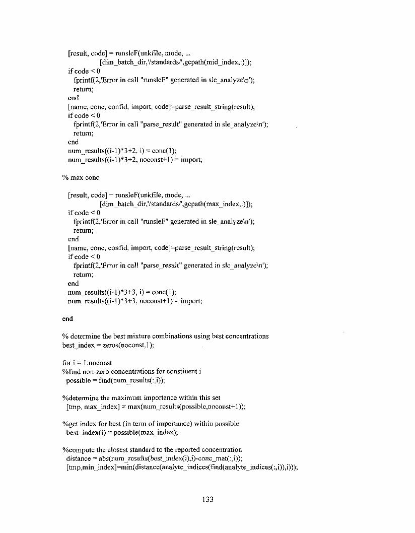
[result, code] = runsleF(unkfile, mode, ...
if code < 0 fprintf(2,'Error in call "runsleF" generated in sle-analyze\n'); return;
[dim-batch_dir,'/standards/',gcpath(mid_index,:)]);
end [name, conc, confid, import, code]=parse-result-string(resu1t); if code < 0
fprintf(2,'Error in call "parse-result" generated in sle - analyze\n'); return;
end num-results((i-l)*3+2, i) = conc( 1); num-results((i- 1)*3+2, noconst+l) = import;
% max conc
[result, code] = runsleF(unkfile, mode, ... [ dim-batch-dir,'/standards/',gcpath(max_index, :)I);
if code < 0 fprintf(2,'Error in call r'runsleF'I generated in sle-analyzeh'); return;
end [name, conc, confid, import, code]=parse-result-string(resu1t); if code < 0
fprintf(2,'Error in call "parse-result" generated in sle-analyzeh'); return;
end num-results((i-l)*3+3, i) = conc( 1); num - results((i-l)*3+3, noconst+l) = import;
end
% determine the best mixture combinations using best concentrations best - index = zeros(noconst, 1);
for i = 1:noconst %find non-zero concentrations for constiuent i
possible = find(num-results(:,i));
%determine the maximum importance within this set [tmp, max - index] = max(num-results(possible,noconst+ 1));
%get index for best (in term of importance) within possible best-index( i) = possible(max_index);
%compute the closest standard to the reported concentration distance = abs(num-results(best-index(i),i)-conc-mat($)); [tmp,min~index]=min(distance(analyte~indices(find(analyte~indices( :,i)),i)));
133

conc-mat( 1 ,:) = fscanf(batfile,'%P ,[ 1 ,noconst]); gcunits = fscanf(batfile,'%s', 1); if nostand > 1
for i=Z:nostand; tmpfile = fscanf(batfile,'%s', 1); gcpath = str2mat(gcpath,tmpfile); conc-rnat(i,:) = fscanf(batfile,'%f,[ 1 ,noconstJ); gcunits = fscanf(batfile,'%s',l );
end end
fclose( batfile); YO determine the best single analyte concentration levels
% determine the concentration range on the standards
analyte-indices = zeros(nostand, noconst); for i = 1:noconst
tmp-vec = find(conc-mat(:,i)); analyte-indices( 1 : length(tmp-vec),i) = tmp-vec;
end
num-results = zeros(3 *noconst, noconst+l);
for i = 1:noconst [tmp, min-index] = min(conc-mat(find(conc-mat(:,i)),i)); min-index = analyte-indices(min I index$); [tmp, max-index] = max(conc-mat(find(conc-mat(: ,i)),i)); max-index = analyte-indices(max-index& mid-index = round((min-index + max-index)/2.0);
% min conc
[result, code] = runsleF(unkfile, mode, _..
if code < 0 fprintf(2,'Error in call "runsleF" generated in sle-analyzeW); return;
[dim - batch-dir,'/standards/',gcpath(min-index,: j]);
end [name, conc, confid, import, code]=parse-result-string(resultj; if code < 0
fprintf(2,'Error in call "parse-result" generated in sle-analyzeh'); return;
end num-results((i- 1 j*3+l, i) = conc( 1); num-results((i- 1)*3+1, noconst4-1) = import;
% middle conc
132

fprintf(2,'Incorrect number of arguments, need unknown file and plot mode.\n'); return;
end;
% Read in *.calset file to determine the standards available. %First find the file in the standards directory calset-file = Is( [dim-batch-dir, '/standards/* .calset']); calset-file = fliplr(deblank(fliplr(deblank(calset-file)))); if length(ca1set-file) -= 0
if abs(calset_file(length(calset-file))) == 10 % new line
end
code = -270; fprintf(2,'Did not find any "*.calset" files in %s.\n', ...
return;
calset-file = calset-file( 1 : length(ca1set-file)- 1 );
% error - could not find any *.calset files else
[dim-batch - dir, '/standards/']);
end;
batfile = fopen(ca1set-file, Y); if batfile = - 1 % check for valid file
code = -900; fprintf(2, 'File not found:%sW,calset-file); return;
end;
noconst = fscanf(batfile, '%g\n', 1); nostand-str = fgetl(batfi1e); nostand = sscanf(nostand-str, '%g', 1);
if noconst < min-const I noconst > max-const I nostand < (noconst * min - stand) code = -272; fprintf(2,'Check the contents of %s, improper number of analytes or standards .W,...
return; calset-file);
end;
for k = 1 :noconst; dummyname = fscanf(batfile, '%SI, 1); anal-names = str2mat(anal_narnes, dummyname);
end; anal-names = anal-names(2:noconst+l,:);
conc-mat = zeros(nostand, noconst);
% read in the standard files and the corresponding concentrations % read in first file tmptile = fscanf(batfile,'%s', 1); gcpath = str2mat(tmpfile);
131

% Instrumentation and Controls Division % Oak Ridge National Laboratory % % Oak Ridge, TN 37831-6011 % Initially created: 7/9/96 YO Last Modified: 7/12/96 MAH YO % Function call: % % [result, code]= sle-analyze(unkfile, mode); % YO This function returns the following variables: % result YO % % YO % YO "1242 6.75e4-02 6.23e+1 1254 -2.33e-02 1.23e-01" % code The integer execution code; zero indicates normal execution. % % The function requires the following input parameters: % unkfile The partial or full pathname of the unknown data file. % The full pathname must start fiom the root file system. % If a partial pathname is passed this must be the *.d segment;
P.O. Box 2008, MS 601 1
A string variable containg the results. The format of
anal yte-name anal yte-conc conc-confid information within the string is:
For multiple analytes this format is repeated for each analyte. For example, assume two analytes are included in the PCR calibration model, the returned string contains:
% % mode A graphics mode flag: YO % % %
the actual filename *.CDF.blr is generated from *.d.
- 1 indicates plot and return immediately, 0 indicates do not plot, and 1 indicates plot and pause for 10 seconds.
min-const = 1; % Minimum nuber of constituents (analytes) mm-const = 4; % Maximum nuber of constituents (analytes) min - stand = 2; % Minimum number of standards per analyte
code = 0; result = [I; perm = [O 1 4 1 I];
% get batch directory [dim-batch-dir, code] = dim-getenv('DIMl3ATCH-DIR'); if code -= 0 % error condition
end return;
if nargin rr= 2 code = -266;
130

'if ac42 is present and ac54 is absent and ac60 is present and import is high then
'if ac42 is present and ac54 is absent and ac60 is present and import is medium then
'if ac42 is present and ac54 is absent and ac60 is present and import is low then
'if ac42 is present and ac54 is absent and ac60 is absent and import is high then
'if ac42 is present and ac54 is absent and ac60 is absent and import is medium then
'if ac42 is present and ac54 is absent and ac60 is absent and import is low then
'if ac42 is absent and ac54 is present and ac60 is absent and import is high then
'if ac42 is absent and ac54 is present and ac60 is absent and import is medium then
'if ac42 is absent and ac54 is present and ac60 is absent and import is low then
'if ac42 is absent and ac54 is absent and ac60 is present and import is high then
'if ac42 is absent and ac54 is absent and ac60 is present and import is medium then
'if ac42 is absent and ac54 is absent and ac60 is present and import is low then
'if ac42 is absent and ac54 is absent and ac60 is absent and import is high then
'if ac42 is absent and ac54 is absent and ac60 is absent and import is medium then
'if ac42 is absent and ac54 is absent and ac60 is absent and import is low then pcr-r - weight
pcr-r-weight is one ';
pcr-r-weight is half ';
pcr-r-weight is zero ';
pcr-r-weight is half ';
pcr-r-weight is zero ';
pcr-r-weight i s zero ';
pcr-r-weight is half ';
pcr-r-weight is zero ';
pcr-r-weight i s zero ';
pcr-r-weight is half I;
pcr-r-weight is zero ';
pcr-r-weight is zero ';
pcr-r-weight is one ';
pcr-r-weight is half ';
is zero 'I;
pcr-r-fis = parsrule(pcr-r-fis, ruleTxt);
writefis(pcrr-fis,'pcr-r');
sle-ana1yze.m function [result, code]= sle-analyze(unkfile, mode);
% FILENAME sle-ana1yze.m Y O
% MATLAB function which determines the optimum combination of individual % standard file to pass to the "runsleF" function based on the importance % parameter. This function will use the *.calset file contained in the % standards subdirectory of the current batch directory (as defined by the % DIMBATCH-DIR). YO YO Written by: Martin Hunt
129

pcr -- r fis = addmf(pcr -- r fis, 'input',l,'present','gauss2mf J0.03 0.1 0.6795 2.21);
%Arocfor 1254 pcr-r-fis = addvar(pcr-r-fis,'input','ac54', [0 21);
pcr -- r fis = addmf(pcr-r-fis, 'input',2,'absent','gauss2mf J0.02378 0 0.03 0.021); pcr-r-fis = addmf(pcr-r-fis, 'input',2,'present','gauss2mf J0.03 0.1 0.6795 2.21);
%Aroclor 1260 pcr-r-fis = addvar(pcr~r~fis7'input','ac60',[0 21);
pcr -- r fis = addmf(pcr-r-fis, 'input',3 ,'absent','gauss2mf J0.023 78 0 0.03 0.021); pcr-r - fis = addmf(pcr-r-fis, 'input',3,'present','gauss2mf ,[0.03 0.1 0.6795 2.21);
%Importance pcr -- r fis = addvar(pcr-r-fis,'input','import',E- 1 11);
pcr-r-fis = addmf(pcr -- r fis, 'input',4,'low','gauss2mf ,[0.34 -1.1 0.1 0.01); pcr-r fis = addmf(pcr r-fis, 'input',4,'mediurn','gauss2mf',[0.2 0.4 0.2 OS]); pcr-rIfis = addmf(pcr_r_fis, 'input',4,'high','gauss2mf ,[O. 1 0.9 0.34 1.11);
%Output variables
pcr-r-fis = addvar(pcr-r-fis,'output','pcr-r-weight', [-0 -4 1 .4]);
pcr-r-fis = addmf(pcr-r-fis, 'output', 1 ,'zero','trimf,[-0.3 5 0 .3 51); pcr-r-fis = addmf(pcr-r-fis, 'output', 1,'half ,'trimf',[O. 15 0.5 0.851); pcr -- r fis = addmqpcr-r-fis, 'output', l,'one','trimf',[O.65 1 .O 1.35 1);
ruleTxt=rif ac42 is present and ac54 is present and ac60 is present and import is high then pcr-r-weight is one ';
'if ac42 is present and ac54 is present and ac60 is present and import is medium then pcr-r-weight is half;
'if ac42 is present and ac54 is present and ac60 is present and import is low then pcr-r-weight is zero ';
'if ac42 is present and ac54 is present and ac60 is absent and import is high then pcr-r-weight is one ';
'if ac42 is present and ac54 is present and ac60 is absent and import is medium then pcr-r-weight is half ';
'if ac42 is present and ac54 is present and ac60 is absent and import is low then pcr-r-weight is zero ';
'if ac42 is absent and ac54 is present and ac60 is present and import is high then pcr-r-weight is one I;
'if ac42 is absent and ac54 i s present and ac60 is present and import is medium then pcr-r-weight is half ';
'if ac42 is absent and ac54 is present and ac60 is present and import is low then pcr-r-weight is zero ';
128

'if ac42 is present and ac54 is absent and ac60 is absent and import is high then
'if ac42 is present and ac54 is absent and ac60 is absent and import is medium then
'if ac42 is present and ac54 is absent and ac60 is absent and import is low then
'if ac42 is absent and ac54 is present and ac60 is absent and import is high then
'if ac42 is absent and ac54 i s present and ac60 is absent and import is medium then
'if ac42 is absent and ac54 is present and ac60 is absent and import is low then
'if ac42 is absent and ac54 is absent and ac60 is present and import is high then
'if ac42 is absent and ac54 is absent and ac60 is present and import is medium then
'if ac42 is absent and ac54 is absent and ac60 is present and import is low then
'if ac42 is absent and ac54 is absent and ac60 is absent and import is high then
'if ac42 is absent and ac54 is absent and ac60 is absent and import is medium then
'if ac42 is absent and ac54 is absent and ac60 is absent and import is low then pcrj-weight
pcrj-weight is half ';
pcrj-weight is zero I ;
pcrg-weight is zero ';
pcrg-weight is half I;
pcrg-weight is zero ';
pcrg-weight is zero ';
pcrg-weight is half ';
pcrj-weight is zero ';
pcrg-weight is zero I;
pcrj-weight is one ';
pcrg-weight is half ';
is zero 'I;
pcrg-fis = parsrule(pcrq-fis, ruleTxt);
pcr - r-fu2zy.m % Generate a Fuzzy inference system % For PCR method based on raw chromatogram signal
% define the threshold for absence vs. presence for Aroclor concentration absgres-thresh = 0.05;
%define the threshoIds for importance - low, medium, high imp-low-med = 0.15; imp-med-high = 0.70;
% generate a Fuzzy inference system pcr-r-fis = newfis('pcr-r','mamdani');
% add input variables YoAroclor 1242 pcr -- r fis = addvar(pcr-r-fis,'input','ac42',[0 21);
per -- r fis = addmf(pcr-r-fis, 'input', l,'absent','gauss2mf' ,[0.02378 0 0.03 0.021);
127

pcrj-fis = addrnftpcrj-fis, 'input',2,'presentf,'gauss2mf ,[0.03 0.1 0.6795 2.21);
%Aroclor 1260 pcrj-fis = addvar(pcrq~fis,'inp~t','ac60'~ [0 21);
pcrq-fis = addmf(pcr2 fis, 'input',3,'absent','gauss2mf ,[0.02378 0 0.03 0.021); pcrj-fis = addmf(pcrjIfis, 'input',3,'presentf,'gauss2mf J0.03 0.1 0.6795 2.21);
%Importance pcrj-fis = addvar(pcr2-fis,'input','import', [- 1 1 I);
pcrg-fis = addmf(pcrj-fis, 'input',4,'low','gauss2mf ,[0.34 -1.1 0.1 0.01); pcrj-fis = addmqpcrj-fis, 'inp~t',4,'medium','gauss2mf ,[0.2 0.4 0.2 O S ] ) ; pcrj-fis = addmqpcrj-fis, 'input',4,'high','gauss2mf ,EO. I 0.9 0.34 1.1 I);
%Output variables
pcrq-fis = addvar(pcrq~fis,'output','pcrj~weight', [ -0.4 1.41);
pcrj-fis = addmf(pcrj-fis, 'output', 1 ,'zero','trimf,[-0.35 0 .35]); pcrj-fis = addmf(pcrj-fis, 'output', 1,'half ,'trimf ,[O. 15 0.5 0.851); pcrg-fis = addmf(pcrj-fis, 'output', l,'one','trimf',[0.65 1 .O 1.351);
ruleTxt==['if ac42 is present and ac54 is present and ac60 is present and import is high then pcrj-weight is one I;
'if ac42 is present and ac54 is present and ac60 is present and import is medium then pcrj-weight i s half;
'if ac42 is present and ac54 is present and ac60 is present and import is low then pcrg-weight is zero ';
'if ac42 is present and ac54 is present and ac60 is absent and import is high then pcrj-weight is one ';
'if ac42 is present and ac54 is present and ac60 is absent and import is medium then pcrj-weight is half ';
'if ac42 is present and ac54 is present and ac60 is absent and import is low then pcrj-weight is zero ';
'if ac42 is absent and ac54 is present and ac60 is present and import is high then pcrj-weight is one ';
'if ac42 is absent and ac54 is present and ac60 is present and import is medium then pcrj-weight is half ';
'if ac42 is absent and ac54 is present and ac60 is present and import is low then pcrg-weight is zero
'if ac42 i s present and ac54 is absent and ac60 is present and import is high then pcrj-weight is one ';
'if ac42 is present and ac54 is absent and ac60 is present and import is medium then pcrg-weight is half ';
'if ac42 is present and ac54 is absent and ac60 is present and import is low then pcrj-weight is zero ';
126

sscanf(str-result( space-indices( I ):len),'%f ?2); if isempty(errmsg) 1
fprjntf(2, 'Error in sscanf %s\n',enmsg); code = -952; return;
end conc = [conc value( l)]; confid = [confid value(2)I; nextindex = space indices( 1)fnext; space-indices = fiidstr(str-resuIt(nextindex:import - start),' I);
space-indices = space-indices + nextindex - 1 ; numana = numana + 1 ;
end
%now get importance
import = sscanf(str-resuIt(import-start:len),'Importance = %f);
name = name(2:numana+l,:); conc = conc'; confid = confid';
return;
pcrj-fuzzy.m % Generate a Fuzzy inference system % For PCR method based on peak area input
% define the threshold for absence vs. presence for Aroclor concentration absgres-thresh = 0.05;
%define the thresholds for importance - low, medium, high imp-low-med = 0.15; imp-med-high = 0.70;
Yo generate a Fuzzy inference system pcry-fis = newfis('pcr_p','mamdani');
% add input variables %Aroclor 1242 pcrq-fis = addvar(pcr_p~fiis,'input','ac42',[0 21);
p c r j - fis = addmf(pcrq fis, 'input', 1 ,'absent','gauss2mf ,[0.02378 0 0.03 0.021); pcrj-fis = addmf(pcrjIfis, 'input', 17'present','gauss2mf ,[0.03 0.1 0.6795 2.21);
%Aroclor 1254 pcrj-fis = addvar(pcrq-fis,'input','ac54',[0 21);
pcrg-fis = addmf(pcr_p_fis, 'input',2,'absent','gaussZmf J0.023 78 0 0.03 0.021);
125

% name A vector of the analyte names. YO % conc A vector of corresponding concentrations % % confid A vector of corresponding confidence intervals % % import A scalar of the importance parameter % % code The integer execution code; zero indicates normal execution. % % The function requires the following input parameters: % str-result A string variable containg the results. The format of % % analyte-name analyte-conc conc-confid importance % % YO item in the string) % % %
information within the string is:
For multiple analytes this format is repeated for each analyte. (with the exception of the importance, which is always the last
For example, assume two analytes are included in the PCR calibration model, the returned string contains:
"1242 6.75e+02 6.23et-l 1254 -2.33e-02 1.23e-01"
code = 0;
lea = length(srr-result); % determine where the spaces are space-indices = findstr(str-result,' ');
% determine where Importance is
import-start = findstr(str-result,'Importance = ');
if isernpty(import-start) u= 0 Yo invalid format for result string code = -95 1; return;
end
nextindex = 1 ; numana = 0; while nextindex < import-start, % read in analyte names
[value, count, errmsg, next] = ...
if isempty(errmsg) -= 1 sscanf( str-result(nextindex:space-indices( 1 )),'%st);
fprintf(2, 'Error in sscanf%s\n',emsg); code = -952; return;
end name = str2mat(name,value); [value, count, errmsg, next] = _..
124
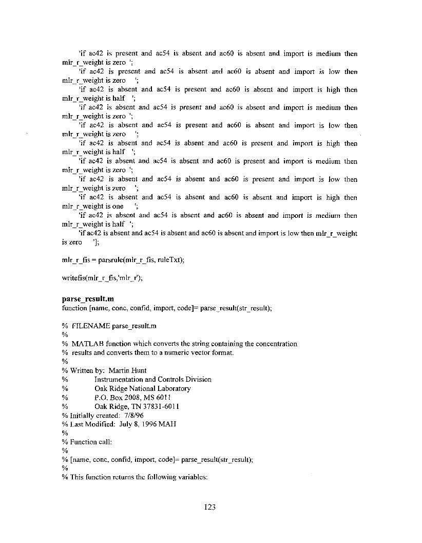
'if ac42 is present and ac54 is absent and ac60 is absent and import is medium then
'if ac42 is present and ac54 is absent and ac60 is absent and import is low then
'if ac42 is absent and ac54 is present and ac60 is absent and import is high then
'if ac42 is absent and ac54 is present and ac60 is absent and import is medium then
'if ac42 is absent and ac54 is present and ac60 is absent and import is low then
'if ac42 is absent and ac54 is absent and ac60 is present and import is high then
'if ac42 is absent and ac54 is absent and ac60 is present and import is medium then
'if ac42 is absent and ac54 is absent and ac60 is present and import is low then
'if ac42 is absent and ac54 is absent and ac60 is absent and import is high then
'if ac42 is absent and ac54 is absent and ac60 is absent and import is medium then
'if ac42 is absent and ac54 is absent and ac60 is absent and import is low then mlr-r-weight
mlr - r-weight is zero I;
mlr-r-weight i s zero ';
mlr-r-weight is half ';
mlr - r-weight is zero I;
mlr -- r weight is zero
mlr _ _ r weight is half I;
mlr-r-weight is zero ';
mlr-r-weight is zero ';
mlr - r-weight is one ';
mlr-r-weight is half ';
is zero '3;
';
mlr-r-fis = parsrule(mlr-r-fis, ruleTxt);
writefis(m lr-r-fis,'mlr-r');
parse-resu1t.m function [name, conc, confid, import, code]= parse-result(str-result);
% FILENAME parse-resu1t.m % % MATLAB function which converts the string containing the concentration % results and converts them to a numeric vector format. % % Written by: Martin Hunt % Instrumentation and Controls Division % Oak Ridge National Laboratory % P.O. Box 2008, MS 601 1 % Oak Ridge, TN 3783 1-601 1 'YO Initially created: 7/8/96 'YO Last Modified: July 8, 1996 MAH % YO Function call: % % [name, conc, confid, import, code]= parse-result(str-result); % % This function returns the following variables:
123

%Aroclor 1260 mlr-r-fis = addvar(mlr~r~fis,'input','ac60',[0 21);
mlr r fis = addmf(m1r r-fis, 'input',3,'absent','gauss2rnf ,[0.02378 0 0.03 0.021); mlr-r-fis -- = addmf(mlrIr-fis, 'inputf,3,'present','gauss2rnf ,[0.03 0.1 0.6795 2.21);
%Importance mlr-r-fis = addvar(m1r-r-fis,'input','import',[- 1 11);
mlr r fis = addmf(mlr-r-fis, 'input',4,'low','gauss2mf,[O.34 -1.1 0.1 0.01); rnlr-r-fis = addmf(m1r r fis, 'input',4,'1pedium','gauss2mf ,[0.2 0.4 0.2 0.51); mlr-r-fis -- = addmf(mlr_rfis, 'input',4,'high','gauss2mf,[O. 1 0.9 0.34 1.11);
%Output variables
m lr-r-fis = addvar( m lr-r-fi s, 'output','m Ir-r-weight' , [ - 0.4 1.41);
mlr-r-fis = addmf(mlr-r-fis, 'output',l ,'zero','trimf,[-0.35 0 -3 51); mlr-r-fis = addmflmlr-r-fis, 'output', 1 ,'half','trimf ,[O. 15 0.5 0.851); mlr - - r fis = addmf(m1r-r-fis, 'output',l ,'one','trimf ,[0.65 1 .O 1.351);
ruleTxt==['if ac42 is present and ac54 is present and ac60 is present and import is high then rnlr-r-weight is one ';
'if ac42 is present and ac54 is present and ac60 is present and import is medium then mlr-r-weight is half;
'if ac42 is present and ac54 is present and ac60 is present and import is low then mlr -- r weight is zero ';
'if ac42 is present and ac54 is present and ac60 is absent and import is high then mlr-r-weight is one ';
'if ac42 is present and ac54 is present and ac60 is absent and import is medium then mlr-r-weight is half I;
'if ac42 is present and ac54 is present and ac60 is absent and import i s low then mlr-r-weight is zero ';
'if ac42 is absent and ac54 is present and ac60 i s present and import is high then mlr-r-weight is one ';
'if ac42 is absent and ac54 is present and ac60 is present and import is medium then mlr-r-weight is half ';
'if ac42 is absent and ac54 is present and ac60 is present and import is low then mlr-r-weight is zero ';
'if ac42 is present and ac54 is absent and ac60 is present and import is high then mlr-r-weight is one ';
'if ac42 is present and ac54 is absent and ac60 is present and import is medium then mlr-r-weight is half ';
'if ac42 is present and ac54 is absent and ac60 is present and import is low then mlr-r-weight is zero ';
'if ac42 is present and ac54 is absent and ac60 is absent and import is high then mlr c r-weight is half ';
122

m l r q fis = addmf(m1rq-fis, 'input',2,'mediurn','gauss2mf J0.2 0.4 0.2 0.51); mlrjLfis = addmf(mlrg-fis, 'input',2,'high','gauss2mf ,[O. 1 0.9 0.34 1.11);
%Output variables
m l r g - fis = addvar(mlrg~fis,'output','mIr~p-weight',[-0.4 1.41);
m l r q fis = addmf(m1rq-fis, 'output', l,'zero','trimf ,[-0.35 0 .35]); r n l r g f i s = addmf(m1rj-fis, 'output',l,'half,'trimf,[O.15 0.5 0.851); mlrgf i s - = addmf(m1rj-fis, 'output',l,'one','trimf ,[0.65 1 .O 1.351);
ruleTxt=['if anal is present and import is high then m l r g - weight is one '; 'if anal is present and import is medium then m l r g - weight is half; 'if anal is present and import is low then mlrg-weight is zero '; 'if anal is absent and import is high then mlrg-weight is one '; 'if anal is absent and import is medium then mlrj-weight is half '; 'if anal is absent and import is low then mlrg-weight is zero 'I;
mlrq-fis = parsrule(m1rg-fis, ruleTxt);
writefis(mlrq_fis,'mIrp');
mlr-r-fuzzy.m % Generate a Fuzzy inference system % For MLR method based on raw chromatogram signal
% define the threshold for absence vs. presence for Aroclor concentration absgres-thresh = 0.05;
%define the thresholds for importance - low, medium, high imp - low-med = 0.15; imp-med-high = 0.70;
% generate a Fuzzy inference system mlr-r-fis = newfis('m1r-r','mamdani');
% add input variables %Aroclor 1242 mlr-r-fis = addvar(mlr-r-fis,'input','ac42',[0 21);
mlr r fis = addmf(m1r-r-fis, 'input',l ,'absent1,'gauss2mf ,[0.02378 0 0.03 0.021); mlr-r-fis -- = addmf(m1r-r-fis, 'input', 1 ,'present','gauss2mf,[0.03 0.1 0.6795 2.21);
%Aroclor 1254 m lr-r-fi s = addvar( m 1 r-r-fi s,' input' ,lac 5 4' , [ 0 21);
mlr r fis = addmf(mlr-r-fis, 'input',2,'absent','gauss2mf ,[0.023 78 0 0.03 0.021); rnlr-r-fis - - = addmf(m1r -- r fis, 'input',2,'present','gauss2mf J0.03 0.1 0.6795 2.21);
121

% % code The integer execution code; zero indicates normal execution. % , % The function requires the following input parameters: % noconst An integer specifying the number of constituents
code = 0;
if noconst = 1 matrix = [J;
elseif noconst 2 matrix = [l I];
elseif noconst == 3 matrix = [l 1 0; 1 0 1; 0 1 1; 1 1 I];
elseif noconst = 4 matrix=[l 100 ;1010 ;1001 ; ...
0 1 1 0; 0 1 0 1; ... 0 0 1 1; ... 1 1 10; 1 0 1 1; ... 0 1 1 1 ; l 1 1 11;
end return;
mlr_p-fuzzy.m YO Generate a Fuzzy inference system % For MLR method based on peak area input
'YO define the threshold for absence vs. presence for Aroclor concentration absgres-thresh = 0.05;
%define the thresholds for importance: - low, medium, high imp-low-med = 0.15; imp-med-high = 0.70;
Yo generate a Fuzzy inference system mlrj-fis = newfis('mlrp','mamdani');
% add input variables %Analyte mlrj-fis = addvar( mlrj-fi s ,' input' ,'anal', 10 21);
m l r q - fis = addmf(mlr_p_fis, 'input',l,'absent','gauss2mf ,[0.02378 0 0.03 0.021); mlrg-fis = addmf(mlrg_fis, 'input', l,'present','gausBmf J0.03 0.1 0.6795 2.21);
%Importance mlrj-fis = addvar(m1rg-fis,'input','import',[- 1 11);
m l r g - fis = addmf(mlrpfis, 'input',2,'low','gauss2mf J0.34 - 1.1 0.1 O.O]);
120
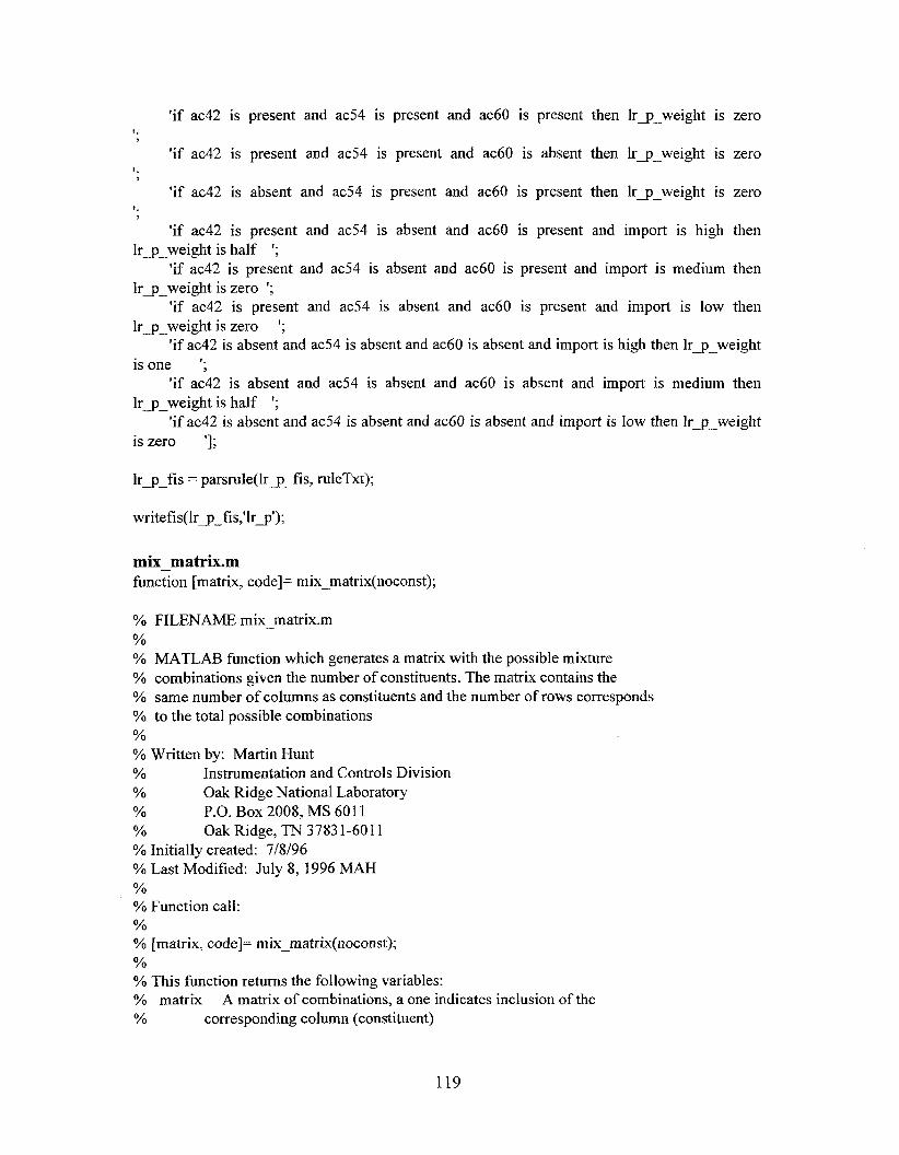
'if ac42 is present and ac54 is present and ac60 is present then lrg-weight is zero
'if ac42 is present and ac54 is present and ac60 is absent then lrg-weight is zero
'if ac42 is absent and ac54 is present and ac60 is present then lrg-weight is zero
'if ac42 is present and ac54 is absent and ac60 is present and import is high then
'if ac42 is present and ac54 is absent and ac60 is present and import is medium then
'if ac42 is present and ac54 is absent and ac60 is present and import is low then
'if ac42 is absent and ac54 is absent and ac60 is absent and import is high then lrq_weight
'if ac42 is absent and ac54 is absent and ac60 is absent and import is medium then
'if ac42 is absent and ac54 is absent and ac60 is absent and import is low then Irj-weight
I . Y
I. 7
I. 7
lrj-weight is half I;
l r q - weight is zero I;
l r g - weight is zero
is one I;
lr-p-weight is half I ;
is zero 'I;
I;
lrg-fis = parsrule( lrj-fis, ruleTxt);
writefis( lrg-fis,'lrj');
mix - matrix.m function [matrix, code]= mix-matrix(noconst);
% FILENAME mix-matrix.m YO YO MATLAB function which generates a matrix with the possible mixture YO combinations given the number of constituents. The matrix contains the YO same number of columns as constituents and the number of rows corresponds % to the total possible combinations % % Written by: Martin Hunt YO Instrumentation and Controls Division YO Oak Ridge National Laboratory YO YO YO Initially created: 7/8/96 % Last Modified: July 8, 1996 MAH YO % Function call: YO % [matrix, code]= mix-rnatrix(noconst); YO YO This function returns the following variables: YO matrix YO corresponding column (constituent)
P.O. Box 2008, MS 601 1 Oak Ridge, TN 37831-601 1
A matrix of combinations, a one indicates inclusion of the
119
l r j I fis = addmf(lrg_fis, 'input', 1 ,'present','gauss2mf ,[0.03 0.1 0.6795 2.23);
%Aroclor 1254 lrq-fis = addvar(1rg - fis,'input','ac54',[0 21);
l r g fis = addmf(1rg-fis, 'input',2,'absent','gauss2mf ,[0.02378 0 0.03 0.021); I r j I f i s = addmf(1rj-fis, 'input',2,'present','gauss2mf ,[0.03 0.1 0.6795 2.21);
%Aroclor 1260 Irj-fis = addvar(lrj~fis,'input,'ac607[0 21);
Irj-fis = addmf(lrg_fis, 'input',3,'absent','gauss2mP ,[0.02378 0 0.03 0.021); l r j I fis = addmf(lrj-fis, 'input',3,'present','gauss2mf,[0.03 0.1 0.6795 2.21);
%Importance l r j - f is = addvar(1rg-fis,'input','import',[- 1 11);
l r j - f is = addmf(1rj-fis, 'input',4,'low','gauss2mf ,[0.34 - 1.1 0.1 0.01); Irq fis = addmf(1rj-fis, 'input',4,'medium','gauss2mf7[0.2 0.4 0.2 0.53); 1rj;fis = addmf(1rj-fis, 'input',4,'high','gauss2mf ,[O. 1 0.9 0.34 1.11);
%Output variables
Irg-fis = addvar(lrj~fis,'output','lr~~weight',[-0.4 1.41);
Irj-fis = addmf(lrj-fis, 'output', 1 ,'zero','trimf ,[-0.35 0 .35]); l r g fis = addmf(1rg-fis, 'output',l,'half,'trimf,[O.15 0.5 0.851); I r g _ f i s = addmf(1rj-fis, 'output', l,'one','trimf',[0.65 1 .O 1.351);
ruleTxt=('if ac42 is present and ac54 is absent and ac60 is absent and import is high then lrg-weight is one ';
'if ac42 is present and ac54 is absent and ac60 is absent and import is medium then Irg-weight is half I;
'if ac42 is present and ac54 is absent and ac60 is absent and import is low then lrg-weight is zero ';
'if ac42 is absent and ac54 is present and ac60 is absent and import is high then lrj-weight is one ';
'if ac42 is absent and ac54 is present and ac60 is absent and import is medium then lrj-weight is half ';
'if ac42 is absent and ac54 is present and ac60 is absent and import is low then lrg-weight is zero ';
'if ac42 is absent and ac54 is absent and a d 0 is present and import is high then lrg-weight is one I;
'if ac42 is absent and ac54 is absent and ac60 is present and import is medium then lrj-weight is half ';
'if ac42 is absent and ac54 is absent and ac60 is present and import is low then Irg-weight is zero ';
118

[dim~batch~dir,'/sofare~code/matlab'l,. . . [dim-batch-dir,'/standards'],. . . source, 1);
end % do not run qa calibration check
return;
fis-range.m function [fis-input,code]= fis-range( input, fis)
code = 0; fis-input = input; num-inputs = getfis(fis, 'numinputs');
if length(input) == num-inputs for i = 1 :num-inputs
input-range = getfk(fis,'input',i,'range'); if input(i) < input-range( 1) fis-input(i) = inputrange( 1);
elseif input(i) > input-range(2) fis-input(i) = input-range(?);
end end
else
end return
code = -1;
Irj-fuzzy.m % Generate a Fuzzy inference system % Linear regression using peak area as input
% define the threshold for absence vs. presence for Aroclor concentration absgres-thresh = 0.05;
%define the thresholds for importance - low, medium, high imp-low - med = 0.15; imp-med-high = 0.70;
% generate a Fuzzy inference system lrj-fis = newfis('lrq','mamdani');
% add input variables %Aroclor 1242 Irj-fis = addvar(lrg_fis,'input','ac42',[0 21);
l r q - fis = addmf(1rq - fis, 'inpuf',l,'absent','gauss2mf J0.02378 0 0.03 0.021);
117

dim-batch-dir = dimsetenv('D1MBATCH - DIR');
% preprocess sample
samp-dir = [dim~batch~dir,'/',sample~type,",sample~id,t.d']; source=[ samp_dir,'/',sample_id,'.cd~] code = preprocessgc(source, - 1);
if code < 0 return;
end;
YO perform off scale check
[code, mingts, maxqts] = qa-off-scale([dim-batch-dir,'/',sample_type,'~~], ... [dim-batch-dir,'/sofode/matlab'j, ... [dim-batch-dir,'/standards'],. . . source, 1);
if code < 0 return;
end
% perform rt marker check
[code, distance] = qa-retention-mark( [dim-batch-dir,'/',sample-type,'s'],. ." [dim~batch~dir,'/sofare~code/matlab'], .. . [dim-batch-dir,'/standards'],. .. source, 1);
if code < 0 return;
end
%determine sample type
if strcmp(samp1e-type,'control') YO must run qa calibration check
%analyze sample [result, code] = dim-analyze(samp1e-type, sample-id, comb-mode);
if code < 0 return;
end
%check calibration
[code, known-conc, percent-err] = qa-cal-check(result, ._. [dirn-batch-dir,'/',sample_type,'s'],.. .
116

end
result = sprintf('%g',recovery);
set(O,'Diary','off); return;
dimva1idate.m function code = dim-validate(sample_type, sample-id, comb-mode);
% FILENAME dim-va1idate.m % % MATLAB function which calls the necessary qdvalidation functions. Will % return on first failure. % % Written by: Martin Hunt % Instrumentation and Controls Division % Oak Ridge National Laboratory % % YO Initially created: 9/18/96 % Last Modified: % % Function call: % % code = dim-validate(sample-type, sample-id, comb - mode); % % This function returns the following variables: % code The integer execution code; zero indicates normal execution. % % The function requires the following input parameters: % sample-type A string containing one of the valid AIA sample types % % sample. % % sample-id YO % % return from "dim_getenv('DIMBATCH-DIR). % YO comb-mode % YO
P.O. Box 2008, MS 601 1 Oak Ridge, TN 3783 1-601 1
.
(standard, unknown, control, blank) corresponding to the
A text string specifying the id of the sample to be analyzed. The file should be located in the kmple-type" subdirectory of the current batch processing directory (as defined by the
The type of combination of the results from the various methods (might be just a single method). Numeric value based on enumerated list defined in "general/dim-s1m.h"
YO initialize variables
code = 0;
115

code = -33 1; fprintf( 1, '%s%d\n', 'Error code = I, code ); return;
ltolerance = fscanf(parmfileid, '%g\n', 1); utolerance = fscanf(parmfileid, '%g\n', 1); fclose(parmfi1eid);
else;
end;
YO determine the recovery
samp-dir = sample;
[results, code] = runSUR(name, samp-dir, plot);
YO setup diary YO dir-index = max(findstr(sample,'/')) - 1 ; diaryfile = sample( 1 :dir-index); diaryfile = [diaryfile, 'P, 'surrogate-result.diary']; set(O,'DiaryFile',diaryfile); set(O,'Diary','on');
if code -= 0 fprintf(1, '%s%dW, 'Error code = I, code); set(O,'Dia.ry',toff);retum ;
end
YO parse result string
[analyte-names, conc, conf, importance, code] = ... parse-result-string(resu1ts);
if code u= 0 fprintf( 1, '%s%d\n', 'Error code = I, code); set(O,'Diary','off );return ;
end
fprintf( 1 ,'Recovery limits are %f and %f percent\n',ltolerance,utolerance); recovery = (conc( 1) / amt) * 100; fprintf( 1 ,'Specified amount of %s is %g ng\n',name,amt); fprintf( 1 ,'Actual recovery of %s is %g percentW,name,recovery); obs = conc( 1);
if (recovery > ltolerance) & (recovery
else
utolerance) code = 0;
code = -1;
114

% This function returns the following variables: % code The integer error code, 0 indicates surrogate recovery % % 'YO
% obs The measured concentration of the surrogate in ng. % % recovery The percent recovery of the surrogate. % % This script requires the following input variables: % name YO 'YO amt YO % sample % to be analyzed. % Yo plot A graphics mode flag: % % % %
is within acceptable tollerances, negative value indicates a failure (recovery low or high).
The name of the surrogate in the form of a string
The true amount of the surrogate in the sample in ng
A text string specifying the full pathname to the sample
<O indicates plot and return immediately, =O indicates do not plot, and >O indicates plot and pause the specified seconds.
code = -1;
recovery = 0; result = [I;
obs = -1;
% % Check the number of input arguments. % if nargin -= 4;
fprintf(1, '%sW, 'Wrong number of arguments passed to the function.'); fprintf( 1, '%s%d\n', 'Error code = ', code); return;
code = -330;
end;
YO % Read the recovery limits from the parameter file. % The error limit is defined in terms of the percentage of the % surrogate recovered YO
parmsubdir = [dim_getenv('DIMBATCH_DlR), '/software-code/matlab']; datasubdir = [dim-getenv('DIMBATCH_DlR), '/unknowns']; parmfile = [parmsubdir, I/,, 'surrogate.parm']; parmfileid = fopen(parmfile, 'r'); if(parmfi1eid = -1);
fprintf( 1 , '%s%s%s\n', 'File: ', parmfile, ' could not be opened for reading.');
113

fprintf( 1, '%s%s%s\n', 'Transfer of files to ', dimenv, ' is complete.'); % % Set the group membership on all the files in the new batch subdirectory. %
[unixstatus, unixresult] = unix( rchgrp -R ', caagroup, ' ' , dimenv]); i€(unixstatus -= 0);
fprintf(1 , '%s\n', 'UNIX "chgrp" command failed.'); code = -576; return;
end; f@-intfi( 1, '%s%s%s%sW, 'A11 files in ', dimenv, ...
' have been assigned to group: ', caagroup); % % Move to the ../software-codehnathlab subdirectory and set the matlab path to % include the new directories. %
eval( ['cd ', dimenv, software-code, '/matlab']);
end;
code = set-dimjath; if code < 0
fprintf( I , 'Error in set-dimgath:%d\n'); return;
end, end; return;
dim-test-surrogatem fimction [code, result, obs, recovery] = dim-test-sun-ogate(name, amt, sample, plot) YO FILENAME dim-test-surroate .m % % MATLAB function which calls the necessary function to determine the kvel % of surrogate recovery (runSUR.m). The function returns a padfail code base % on the tolerances specified in the file "surrogate.pann" % % Written by: Martin A. Hunt YO Instrumentation & Controls Divison % Oak Ridge National Laboratory YO P.O. Box 2008 % YO % YO % Function call: % % [code, obs, recovery] = dim-test-surrogate(name, amt, sample, plot) %
Oak Ridge, TN 3783 1-601 1 Initially created: May 1, 1997 Last modified: May 5, 1997
112

[unixstatus, unixresult] = unix( ['chmod 660 ',dimenv,
if(unixstatus -= 0); so ftware-code,'/nn/* '1) ;
fprintf( 1 , '%sW, 'UNIX "chmod" comm-and failed while
code = -572; return;
changing permissions on the ./nn files.');
end; end;
% % Now copy the general files. %
[unixstatus, output] = unix(['ls ', generalcode]); if(unixstatus rr= 0);
fprintf( 1 , '%s\n', 'UNIX "1s" command failed while obtain a listing of the
code = -573; return;
source GENERAL code and parameter files.');
end; if(isempty(0utput) = 1);
fprintf( 1 , '%s%s%s\n', 'Subdirectory ', generalcode, ' is empty!'); fprintf(1, '%sW, 'No files will be copied.');
fprintf( 1, '%s%s%s%s\n', ... else;
'Source "general" code is being copied to the I,... dimenv, software-code, '/general subdirectory.');
nofiles = length(findstr(abs( lo), output)); for k = 1:nofiles;
nullindex = findstr(abs( lo), output); filename = output( 1 :nullindex( 1) - 1); output = output(nullindex( 1) + 1 :length(output)); [unixstatus, unixresult] = unix( ['cp ', generalcode, ...
I/,, filename, ' I,... dimenv, software-code, '/general?, filename]);
fprintf( 1, '%sW, 'UNIX "cp" command failed.'); code = -574; return;
if(unixstatus -= 0);
end; end; [unixstatus, unixresult] = unix( ['chmod 660 ', dimenv,
software-code,'/general/*']); if(unixstatus -= 0);
changing permissions on the general files.'); fprintf( 1, '%sW, 'UNIX "chmod" command failed while
code = -575; return;
end; end;
111

fprintf( 1, '%sW, 'UNIX "cp" command failed.'); code = -568; return;
end; end; [unixstatus, unixresult] = unix(['chmod 660 ',dimenvy '/per/*']); if(unixstatus -.= 0);
fprintf(1, '%sW, 'UNIX 'lchrnod" command failed while changing
code = -569; return;
permission on parameter files.');
end; [unixstatus, unixresult] = unix(['chmod 660 ',dimenv, '/mlr/*']); if(unixstatus 4 0);
fprintf( 1 , '%s\n', 'UNIX "chmod" command failed while changing
code = -569; return;
permission on parameter files.');
end; YO YO Now copy the neural network code and any parameter files. %
[unixstatus, output] = unix([tls ', nncode]); if(unixstatus 0);
fprintf( I , 'YosW, 'UNTX "ls" command failed while obtain a listing of the
code = -570; return;
source NEURAL NETWORK code and parameter files.');
end; if(isempty(output) = 1);
fprintf(1, '%s%s%sW, 'Subdirectory ', nncode, ' is empty!'); fprintf(1, '%s\n', 'No files will be copied.');
fprintf(1, '%s%s%s%s\n', 'Source NN code is being copied to the ', ...
nofiles = length(findstr(abs(lO), output)); for k = I :nofrles;
else;
dimenv, software-de, '/nn subdirectory.');
nullindex = findstr(abs( lo), output); filename = output( 1 :nullindex( 1) - 1); output = output(nullindex( 1) + 1 :length(output)); [unixstatus, unixresult] = unix(['cp ', nncode, ...
' P , filename, ' I , . . .
dimenv, sohare-code, '/nn/', filename]); if(unixstatus u= 0);
fprintf( 1, '%sW, 'UNIX "cp" command failed.'); code = -57 1; return;
end; end;
110
% yields this result independent of the permissions on the source files. %
'/matlab/*']); [unixstatus, unixresult] = unix(['chmod 550 ', dimenv, software-code,
if(unixstatus -= 0); fprintf( 1 , '%s\n', 'UNIX "chmod" failed while setting
code = -567; return;
read and execute file permissions in ../matlab subdirectory.');
end; [unixstatus, unixresult] = unix(['chmod 440 ', dimenv, software-code,
'/matlab/* .m']); if(unixstatus -= 0);
fprintf( 1 , '%s\n', 'UNIX "chmodl' failed while setting read only file permissions in ../matlab subdirectory.');
code = -567; return;
end; [unixstatus, unixresult] = mix( ['chmod 660 ', dimenv, software-code,
'/matlab/* .parm']); if(unixstatus -= 0);
fprintf( 1, '%s\n', 'UNIX "chmod" failed while setting
code = -567; return;
read and write file permissions in ../matlab subdirectory.');
end;
end; % % Put copies of two parameter files into the ../pcr and Jmlr subdirectories. % The copies in ../matlab will be the default files. %
parmfile( 1,:) = 'decimation.parm '; parmfile(2,:) = 'integration.parm'; fprintf(1, '%s\n', 'Coping the relevant parameter files into ../pcr and Jmlr.'); for k = 1 :min(size(parmfile));
filename = deblank(parmfile(k,:)); [unixstatus, unixresult] = unix(['cp I, matlabcode, ...
I/', filename, ... ', dimenv, '/per/', filename]);
fprintf( 1 , '%s\n', 'UNIX "cp" command failed.'); code = -568; return;
if(unixstatus rr= 0);
end; [unixstatus, unixresult] = unix(['cp ', matlabcode, ...
I/', filename, ... ' ', dimenv, '/mlr/', filename]);
if(unixstatus -= 0);
109
code = -563; return;
end; [unixstatus, unixresuk] = mix( ['chmod -R 2770 ',dimenv, software - code]); if(unixstatus -= 0);
fprintf( 1, '%s\n', 'UNIX "chmod" command failed while creating the
code = -564; retum;
new batch subdirectory.');
end; fprintf(1, '%s%s%s\n', 'Creation of the directory structure for ', dimenv, ' is
complete.'); % % Copy the relevant code from the source to the destination directories. % Copy the MATLAB code and parameter files. 'YO
[unixstatus, output] = unix(['ls ', matlabcode]); if(unixstatus u= 0);
fprintf( 1, 'Yosh', 'UNIX "1s" command failed while obtaining a listing of
code = -565; return;
the source MATLAB code and parameter files.');
end; if(isempty(output) == 1);
fprintf( 1, '%s%s%sW, 'Subdirectory I, matlabcode, ' is empty!'); fprintf(1, '%s\n', 'No files will be copied.');
fprintf( 1, '%s%s%s%s\n', ... else;
'Source MATLAB code is being copied to the 1 9 . . .
dimenv, software-code, '/mattab subdirectory.'); nofiles = length(findstr(abs( 1 0), output)); for k = 1:nofiles;
nullindex = findstr(abs( lo), output); filename = output( 1 :nullindex( 1) - 1); output = output(nullindex( 1) + 1 :length(output)); [unixstatus, unixresult] = unix(rcp ', matlabcode, ...
I/,, filename, ' I,... dimenv, software_code, '/matlab/', filename]);
fprintf( 1, '%s\n', 'UNIX "cp" command failed.'); code = -566; return;
if(unixstatus u= 0);
end; end;
YO % Set the file permissions to protect the code in the batch subdirectory. 'YO Only the user and members of the group will have permissions. 'YO MATL,AB M-files have read permission, binary files have read and execute permissions, 'YO and parameter files have read write permissions. The permissions coding
[unixstatus, unixresulst] = unix( ['mkdir I, dimenv, '/mlr']); if(unixstatus -= 0);
fprintf( 1, '%sW, 'UNIX "mkdir" command failed while creating the
code = -557; return;
"mlr" subdirectory.');
end; [unixstatus, unixresult] = unix( ['mkdir I , dimenv, '/nn']); if(unixstatus -= 0);
fprintf( 1, '%s\n', 'UNIX "mkdir" command failed while creating the "nn"
code = -558; return;
subdirectory.');
end; [unixstatus, unixresult] = unix( ['chmod 2770 ',dimenv,'/*']); if(unixstatus -= 0);
fprintf( 1, '%s\n', 'UNIX l'chmod'' command failed while creating the
code = -559; return;
new batch subdirectory.');
end; % % Create the software subdirectories. %
[unixstatus, unixresult] = unix(['mkdir ', dimenv, software-code]); if(unixstatus -= 0);
fprintf( 1, '%ski, 'UNIX "mkdir" command failed while creating the
code = -560; return;
"software-code" subdirectory.');
end; [unixstatus, unixresult] = unix( ['mkdir I , dimenv, software-code, '/matlab']); if(unixstatus -= 0);
fprintf( 1, '%s\n', 'UNIX "mkdir" command failed while creating the
code = -561; return;
"matlab" software subdirectory.');
end; [unixstatus, unixresult] = unix( ['mkdir I, dimenv, software-code, '/nn']); if(unixstatus -= 0);
fprintf( 1 , '%sW, 'UNIX "mkdir" command failed while creating the
code = -562; return;
"neural network" software subdirectory.');
end; [unixstatus, unixresult] = unix( ['mkdir ', dimenv, softwarecode, '/general']); if(unixstatus 0);
fprintf( 1, '%s\n', 'UNIX "mkdir" command failed while creating the "general" software subdirectory.');
107
mystring, is undefined.'); return;
[unixstatus, unixresult] = unix(['chmod 2770 ',dimenv]); if(unixstatus -= 0);
else;
fprintf( 1, '%s\n', 'UNIX "chmod" command failed while creating
code = -551; return;
the new batch subdirectory.');
end; end;
YO YO Create the data subdirectories for the new batch. YO
[unixstatus, unixresult] = unix(['mkdir I, dimenv, '/standards']); if(unixstatus -= 0);
fprintf( 1 , '%s\n', 'UNIX "mkdir" command failed while creating the
code = -552; return;
"standards'' subdirectory.');
end; [unixstatus, unixresult] = unix(fmkdir ', dimenv, '/unknowns']); if(unixstatus 4 0);
fprintf( 1, '%s\n', 'UNIX "mkdir" command failed while creating the
code = -5 53 ; return;
"unknowns" subdirectory.');
end; [unixstatus, unixresult] = unix(['mkdir ', dimenv, '/controls']); if(unixstatus -= 0);
fprintf( 1, '%s\n', 'UNIX "mkdir" command failed while creating the
code = -554; return;
"controls" subdirectory.');
end; [unixstatus, unixresult] = unix(rmkdir ', dimenv, '/blanks']); if(unixstatus a 0);
fprintf( 1, '%s\n', 'UNIX "mkdir" command failed while creating the
code = -555; return;
"blanks" subdirectory.');
end; [unixstatus, unixresult] = unix(['mkdir ', dimenv, '/per']); if(unixstatus -= 0);
fprintf( 1, '%s\n', 'UNIX "mkdir" command failed while creating the
code = -556; return;
"pcr" subdirectory.');
end;
106

fprintf( 1, '%s%s\n', 'The current SAMPLE BATCH DIRECTORY is: I, dimenv); % % Create batch directory environment variable %
dim-setenv('D1MBATCH-DIR, dimenv); [dirstatus, code] = direxist(dimenv); if(code rr= 0);
fprintf( 1 ,'Error in the "direxist" functionh'); return;
end; if(dirstatus == 2);
fprintf( 1 , '%s%s%s\n', 'A directory structure for ', dimenv, ' exists'); fprintf( 1, '%s%s\n', 'The GC DIM will run using code from ', dimenv);
[dirstatus, code] = direxist( [dimenv software-code '/matlab']); if(code -= 0);
fprintf( 1 ,'Error in the "direxist" function\n'); return;
if(dirstatus u= 2); end
fprintf( 1 ,'subdirectory %s%s/matlab does not exist\n', __.
code = -980; return;
dimenv, software-code);
end;
eval(['cd ', dimenv, software-code, '/matlab']); else;
YO % Create the new batch subdirectory. %
fprintf( 1, '%s\n', 'The directory structure for the new batch is being established.');
if(unixstatus -= 0); [unixstatus, unixresult] = unix(['mkdir ', dimenv]);
fprintf( 1, '%sW, 'UNIX "mkdir" command failed while creating the new
mystring = fliplr(dimenv); while(mystring( 1) -= I/');
batch subdirectory.');
mystring = mystring(2:length(mystring)); if(length(mystring) == 0);
fprintf(1, 'Yos%s%sW, ... 'The partial pathname for the batch
subdirectory ', ... dimenv, ' is not defined properly.');
code = -550; return;
end; end; mystring = fliplr(mystring(2: length(mystring))); fprintf(1, '%s%s%s\n', 'A probable cause: Partial pathname ', ...
105

for i = 1:noconst result = [result, ' ', anal-names(i,:), ' ' ,...
sprintf('%- 10.3e', conc(i)), ' ', sprintf('%-l0.3e', confid(i))]; end;
set(0, 'DiaryFile', diaryfle); set(0, 'Diary', 'on'); fprintf(1 ,'Final result:%s\n',result);
set(0, 'Diary', 'off); return;
dim-set-batchm function [code] = dim-set-batch(dimenv) % MATLAB function to setup the batch directories YO This file should be stored in the general control and communication dir. % % Written by: Leon N. Klatt % Robotics & Process Systems Division % Oak Ridge National Laboratory YO P.O. Box 2008 YO % % YO Modified by: Martin Hunt % YO % Modified by: L. N. KIatt November 4, 1996 to make it agree with startup-m % % First define the installation specific paths for the original % source code being used with the batch of samples for the GC DIM. % The following group of lines will require defrnition for each % installation of the GC DIM. % matlabcode = '/caa/dim/gc-dev'; nncode = '/caa/dim/CANNS'; generalcode = '/caa/dim/general'; software-code = '/software-code'; caagroup = 'caa'; % % Start the set up process. % if(dimenv = [I);
Oak Ridge, TN 3783 1-6306 Initially created: February 28, 1995 Last Modified: April 3, 1996
Remove user interaction, create batch directory file Last Modified: July 3 I , 1996
fprintf( 1, '%s\n', 'The variable containing the batch directory is not defined!'); return;
else

elseif comb-mode == 10 % SLE raw fprintfii 1 ,'Combination mode: SLE Raw\n');
% call method
[result, code] = sle-analyze(ful1gath-sample, plotting); if code < 0
return; end;
%parse result
[name, conc, confid, import, code]= parse-result-string(resu1t); if code < 0
return; end;
%check to see which analyte reported
result = [I; for i = 1:noconst
for j = 1 :length(conc) if strcmp(ana1-names(i,:), name6,:))
result = [result, ' ', anal-names(i,:), ' ' ,... sprintf('%- 10.3e', concfi), confidfi))];
else result = [result, ' ', anal-names(i,:), ' ' ,...
sprintf('%- 10.3e', 0.0, - 1 .O)]; end;
end; end; result = [result, ' ', 'Importance = ', sprintf(' %7.3f, ...
result = fliplr(deblank(fliplr(deblank(result)))); result = [result, setstr(0)J;
import)];
%parse complete result
[name, conc, confid, import, code]= parse-result-string(resu1t); if code < 0
return; end;
end; YO % write final result string % result = [I;
103

elseif comb-mode = 5 % PCR peak
% determine the *.peaksetfact file to use fprintf( 1,'Combination mode: PCR PeakW);
modelfile = [calsetgrefix, '.peakset.fact'];
[result, code] = dimpcrcal(modelfile, fullgath-sample, plotting); if code < 0
return; end;
[name, conc, confid, import, code]= parse-result-string(resu1t); if code < 0
return; end;
elseif comb-mode = 6 YO MLR raw
elseif comb-mode = 7 % MLR peak
for i = 1:noconst [result, code] = runMLR(ana1-names&:), fulljath-sample, plotting); [name, tmp-conc, tmp-confid, import, code]= parse-result-string(result); conc( i)--tmp-conc; confid(i)=tmp-confid;
end conc = conc'; confid = confid';
elseif comb-mode == 8 % Linear regression peak
elseif comb-mode = 9 'YO Neural network fprintf( 1 ,'Combination mode: ANN PeakW); network = [dim-batch-dir, '/nn/l,calsetjrefix,'.net'];
[result, code] = ann-analysis(full_path-sample,network,calsetgrefix);
if code < 0 return;
end;
[name, conc, confid, import, code]= parse-result-string(resu1t); if code < 0
return; end;
102

elseif comb-mode == 3 % fusion f$rintf( 1 ,'Combination mode: Fusion\n');
for i = 1 :length(index) if comb-matrix(index(i),3) < 0,
comb-matrix(index(i),3) = 0; elseif comb-matrix(index(i),3) > 1,
comb-matrix(index(i),3) = 1; end;
end;
for i = 1:noconst
index = find(-isnan(comb-matrix( :,((i- 1)*2)+4))); %normalize weights to sum to one
sum-weight = sum(comb~matrix(index,3)); weight-vect = comb-matrix(index,3) / sum-weight;
conc(i) = sum(comb-matrix(index,((i- 1)*2)+4) .* weight-vect);
conf - index = find(comb-matrix(index,((i- 1)*2)+5) -= - 1); sum-weight = sum(comb-matrix( index(conf-index),3)); weight-vect = comb~matrix(index(conf~index),3) / sum-weight; confid(i) = sqrt(sum((comb-matrix(index(c0nf-index),((i- 1)*2)+5) .*2)...
% don't include methods with no confidence interval
. * weight-vect)); end;
end;
fprintf( 1 ,'Summary of combination parameters:\n'); comb-matrix
elseif comb-mode == 4 % PCR raw
% determine the *.calset.fact file to use fprintf( 1 ,'Combination mode: PCR Raw\n');
modelfile = [calsetgrefix, '.calset.fact'];
[result, code] = dimpcrcal(modelfile, fullqath-sample, plotting);
[name, conc, confid, import, code]= parse-result-string(resu1t); if code < 0
return; end;
101

else
end
for i = 1 :noconst
comb~matrix(row~index,3) = 1 .O;
comb-matrix(mw-index,((i- 1)*2)+4) = conc(i); comb-matrix(row-index,((i- 1)*2)+5) = confid(i);
end; YO % end SLE
set(0, 'DiaryFile', diaryfile); set(0, 'Diary', 'on');
YO combine results %
index = find(comb-matrix(:,l));
if comb-mode = 0 % minimum Eprintf( 1 ,'Combination mode: Minimumh');
for i = 1:noconst valid-index = find(-isnan(comb-matrix(index,((i- 1)*2)+4))); [conc(i), pick-index] = rnin(comb-matrix(va1id-index,((i- 1)*2)+4)); confid( i) = comb-matrix(va1id-index(pick-index),((i- 1)*2)+5);
end;
elseif comb-mode = 1 % maximum fprintf( 1 ,'Combination mode: Maximumin');
for i = 1:noconst valid - index = find(-isnan(comb-matrix( index,((i- 1)*2)+4))); [conc(i), pick-index] = max(comb-matrix(va1id-index,((i- 1)*2)+4)); confid( i) = comb-matrix(va1id-index(p ick-index),(( i- 1 ) *2)+ 5) ;
end;
elseif comb-mode = 2 % average fprintfi 1 ,'Combination mode: Averagein');
for i = 1:noconst valid index = find(-isnan(comb-matrix(index,((i- 1)*2)+4))); concci> = mean(comb-matrix(valid-index,((i-l)*2)+4));
conf-index = find(comb-matrix(valid-index,((i-1)*2)+5) -= -1); confid(i) = ...
% don't include methods with no confidence interval
sqrt(mean(comb-matrix(valid-index(conf-index),((i- 1)*2)+5).*2)); end;
1 00

if code < 0 return;
end;
%parse result
[name, conc, confid, import, code]= parse-result-string(resu1t); if code < 0
return; end;
%check to see which analyte reported
result = [I; for i = 1:noconst
match-flag = 0; for j = 1 :length(conc)
if strcmp(ana1-names( i, :), name6 , :)) result = [result, ' ', anal-names(i,:), ,...
sprintf('%-10.3e', concfi)), ', ... sprintf('%- 10.3e', confid(i))];
match-flag = 1 ; end;
end; if match-flag == 0
result = [result, ', anal-names(i,:), ' ' ,... sprintf('%-10.3e7, 0.0, -l.O)];
end; end;
result = [result, ' I , 'Importance = I, sprintf(' %7.3f , ...
result = fliplr(deblank(fliplr(deblank(resu1t)))); result = [result, setstr(0)l;
import)] ;
% now parse result with all analytes
[name, conc, confid, import, code]= parse-result-string(resu1t);
if code < 0 return;
end;
comb-matrix(row-index, 1) = 10; comb-matrix(row-index,2) = import; if comb-mode = 3
%method is SLER %importance is column 2
fis = readfis('s1e-r'); input = fis-range([conc' import], fis); comb-matrix(row-index,3) = evalfis(input, fis);
99

else
end comb-matrix(row-index+i- 1 ,((i- 1)*2)+4) = conc; comb-matrix(row-index+i- 1 ,((i- 1)*2)+5) = confid;
comb - matrix(row-index-ki- 1,3) = 1 .O;
end
% end MLR Peak
row-index = row-index +3;
% Neural network network = [dim-batch-dir, '/nn/',calsetgrefix,'.net'] ;
[result, code] = ann-analysis(fulIgath-sample,network,calsetgrefix);
if code 0 return;
end;
[name, conc, confid, import, code]= parse-result-string(resu1t); if code < 0
return; end;
comb-matrix(row-index, 1) = 9; comb~matrix(row~index,2) = import; if comb-mode == 3
%method is NNP %importance is column 2
f i s = readfis('ann2'); input = fis-range([conc' import], fis); comb~matrix(row~index,3) = evalfis(input, fis);
comb-matrix(row-index,3) = 1 ,O; else
end
for i = 1:noconst comb-matrix(row-index,((i- 1)*2)+4) = conc(i); comb-matrix(row-index,((i- 1)*2)+5) = confid(i);
end; %end ANN
row-index = row-index + 1 ;
%SLE Raw
[result, code] = sle-analyze(ful1gath-sample, plotting);
98

for i = 1:noconst comb-matrix(row-index,(( i- 1)*2)+4) = conc(i); comb - matrix(row-index,((i-1)*2)+5) = confid(i);
end; % % end PCRR
row-index = row-index +I ;
%PCR Peak modelfile = [calsetjrefix, '.peakset.fact']; [result, code] = dimpcrcal(modelfile, fullgath-sample, plotting); [name, conc, confid, import, code]= parse-resuIt-string(resu1t); if code < 0
return; end;
comb-matrix(row-index,l) = 5; comb~matrix(row~index,2) = import; if comb-mode == 3
%method is PCRP %importance is column 2
fis = readfis('pcrq'); input = fis-range([conc' import], fis); comb-matrix(row-index,3) = evalfis( input, fis);
comb~matrix(ro~v~index,3) = 1.0; else
end
for i = 1:noconst comb - matrix( row-index, (( i- 1) *2)+4) = conc( i); comb - matrix(row-index,((i- 1)*2)+5) = confid(i);
end;
% end PCRP
row - index = row-index +l;
%MLR Peak if comb-mode = 3
end fis = readfis('m1rq');
for i = 1 :noconst [result, code] = runMLR(ana1-names(i,:), fullqath-sample, plotting); [name, conc, confid, import, code]= parse-result-string(resu1t); comb-matrix(row-index+i- 1 , 1) = 7; %method is MLR Peak comb - matrix(row-index-ti- 1,2) = import; if comb-mode = 3
input = fis-range([conc' import], fis); comb-matrix(row-index+i- 1,3) = evalfis( input, fis);
97

fprintf( 1,'Check the contents of %s, improper number of analytes or standards .\n',..~
return; calset-file);
end;
% read analyte name strings
for k = 1 :noconst; dummyname = fscanf(batfile, '%SI, 1); anal-names = str2mat(anal-names, dummyname);
end;
anal-names = anal-names(2:noconst+l,:);
fclose(batfi1e);
fprintf( 1 ,'Analysis for the following analytes:\n'); for k = 1 :noconst;
end; fprintf( 1 ,'#%d: %sW,k, anal-names(k,:));
% determine combination mode
if comb-mode >= 0 & comb-mode <= 3 % call all avaiable methods comb-matrix = zeros(6+noconst, 3+2*noconst); %create matrix for results comb-matrix( :,2:3+2*noconst) = ones(6+noconst,2+2 *noconst)*NaN;
row-index = 1 ;
modelfile = [calsetqrefix, '.calset.fact']; [result, code] = dimpcrcal(modelfile, fullqath-sample, plotting); if code < 0
return; end; [name, conc, confid, import, code]= parse-result-string(resu1t); if code < 0
return; end;
%PCR Raw
comb-matrix(row-index, 1) = 4; comb~matrix(row~index,2) = import; if comb-mode = 3
%method is PCRR %importance is column 2
fis = readfistpcr-r'); input = fis-range([conc' import], fis); comb~matrix(row~index,3) = evalfis(input, fis);
comb-matrix(row-index,3) = 1 .O; else
end
96

calset-file = fliplr(deblank(flipIr(deblank(ca1set-file)))); if length(ca1set-file) rr= 0
if abs(ca1set-file(length(ca1set-file))) == 10 % new line
end
code = -470; fprintf(1,'Did not find any "*.calset" files in %s .hi',...
return;
calset-file = calset-file( 1 :length(calset-file)- 1);
% error - could not find any *.calset files else
[dim-batch-dir, '/standards/']);
end;
% extract the prefix of the *.calset file
slash-index = findstr(ca1set-file,'/'); ext-index = findstr(ca1set-file,'.calset');
if isempty(s1ash-index) I isempty(ext-index) I... slash-index(length( slash-index))+l > (ext-index- 1) code = -472; fprintf( 1 ,'Could not isolate the prefix of the *.calset file:%s\n', ...
return; calset-file);
end;
calsetgrefix = calset-file(s1ash-index(length(s1ash-index))+ 1 :(ext - index- 1));
fprintf( 1 ,'Using %s as the calibration set prefix\n', calsetgrefix);
% determine the analyte names
batfile = fopen(ca1set-file, 'r'); if batfile == - 1 % check for valid file
code = -900; fprintf( 1, 'File not found:%s\n',calset-file); return;
end;
% determine the number of standards
noconst = fscanf(batfile, '%gin', 1); nostand-str = fgetl(batfi1e); nostand = sscanf(nostand-str, '%g', 1);
% check the number of standards
if noconst < min-const I noconst > max-const I nostand < (noconst * min-stand) code = -272;
95

% % return from "dim-getenv('D1MBATCH-DIR). % % comb-mode The type of combination of the results from the various methods % %
the current batch processing directory (as defined by the
(might be just a single method). Numeric value based on enumerated list defined in "general/dim-s1m.h"
YO initialize variables
code = 0; result = [I; plotting = 0; %plotting flag as passed to methods min-const = 1; %minimum number of analytes max-const = 3; %maximum number of analytes min-stand = 2; %minimum number of standards
dim-batch-dir = dim_getenv('DIMBATCH-DIR'); if isempty(dim-batch-dir)
code = -473; fprintf( 1 'Batch directory environment variable not set\n'); return;
end
% % check for existence of sample % sample-dir = [sample-id,'.#]; test = Is( [dim-batch-dir, '/',sample-type,'s/',sple - dir]); if isempty(test)
code = -474; fprintf( 1, 'Could not find unknown sample file:%s\n', ...
return; [dim-batch-dir, 'P,sample_type,'sP,sample - dir]);
end;
fullqath-sample = [dim-batch-dir, '~,sample_type,'s~,sample_dir,'P,. .. sample-id,'.cdf. blr'];
%setup diary file diaryfile = [dim-batch-dir,'/',sample-type,'s/',sample-dir,'/', 'dim--analyze.diary']; set(0, 'DiaryFile', diaryfile); set(0, 'Diary', 'on'); datetimestr = time-date(c1ock); fprintf( 1, '%s%sW, 'Sample analyzed on: ', datetimestr);
% Read in *.calset file to determine the prefix. %First find the file in the standards directory
calset-file = Is( [dim-batch-dir, '/standards/* .calset']);
94

calsetgrefix = calset-file( slash-index(length( slash-index))+ 1 :(ext-index- 1));
result = calsetqrefix;
return;
dim - ana1yze.m function [result, code]= dim-analyze( sample-type, sample-id, comb - mode);
% FILENAME dim-ana1yze.m % % MATLAB function which is called by the DIM control code (via the MATLAB % engine) to compute the concentration of desired analytes in the unknown % sample. The function will make the necessary calls to the individual % methods based on the input arguments. % % Written by: Martin Hunt % Instrumentation and Controls Division YO Oak Ridge National Laboratory YO % % Initially created: 7/5/96 % Last Modified: 8/7/96 MAH % % Function call: % % [result, code]= dim-analyze(samp1e-type, sample-id, comb - mode); % % This function returns the following variables: % result % information within the string is: % analyte-name analyteconc conc-confid YO For multiple analytes this format is repeated for each analyte. % For example, assume two analytes are included in the PCR YO calibration model, the returned string contains: YO "1242 6.75e+02 6.23e+1 1254 -2.33e-02 1.23e-01" % % code The integer execution code; zero indicates normal execution. YO % The function requires the following input parameters: % sample-type A string containing one of the valid AIA sample types YO % sample. YO % sample-id YO
P.O. Box 2008, MS 601 1 Oak Ridge, TN 37831-601 1
A string variable containg the results. The format of
(standard, unknown, control, blank) corresponding to the
A text string specifying the id of the sample to be analyzed. The file should be located in the 'tsample-type'l subdirectory of
93

'if ac42 is absent and ac54 is absent and ac60 is absent and import is medium then
'if a d 2 is absent and ac54 is absent and ac60 is absent and import is low then ann>-weight is half ';
anng-weight is zero '3;
anng-fis = parsrule(anng-fis, ruleTxt);
writefis(annq_fis,'annq');
ca1grefix.m function [result, code] = calsrefix();
dim - batch-dir = dim-getenv('DIMBATCH-DIR');
code = 0;
% Read in *.calset file to determine the prefuc. %First find the file in the standards directory
calset-file = Is( [dim-batch-dir, '/standards/* .calset']); calset-file = fliplr(deblank(fliplr(deblank(ca1set-file)))); if length(ca1set-file) -= 0
if abs(calset_fle(length(calset-file))) = 10 % new line
end
code = -470; fprintf(1,'Did not find any "*.calset'' files in %s.\n', ...
return;
calset-file = calset-file( 1 :length(calset-file)-l);
% error - could not find any *.calset files else
[dim-batch-dir, '/standards/']);
end;
% extract the prefix of the * .calset file
slash-index = findstr(ca1set-file,'/'); ext - index = findstr(calset_file,'.calset');
if isempty(s1ashindex) I isempty(ext-index) I... slash - index(length(s1ash-index))+l > (ext - index- 1) code = -472; fprintf( 1,'Could not isolate the prefix of the *.calset file:%s\n', ...
return; calset-file);
end;
92

annq-fis = addmf(ann2-fis, 'output', 1 ,'zero','trimf',[-0.35 0 .35]); a n n q fis = addmf(annq-fis, 'output', 1 ,'half ,'trimf ,[O. 15 0.5 0.851); annq-fis I = addmf(anng-fis, 'output', 1 ,'one','trimf',[0.65 1 .O 1.351);
ruleTxt==['if ac42 is present and ac54 is present and ac60 is present and import is high then a n n q - weight is one I;
'if ac42 is present and ac54 is present and ac60 is present and import is medium then a n n 2 - weight is half;
'if ac42 is present and ac54 is present and ac60 is present and import is low then annq-weight is zero ';
'if ac42 is present and ac54 is present and ac60 is absent and import is high then annq-weight is one ';
'if ac42 is present and ac54 is present and ac60 is absent and import is medium then a n n q - weight is half ';
'if ac42 is present and ac54 is present and ac60 is absent and import is low then anng-weight is zero ';
'if ac42 is absent and ac54 is present and ac60 is present and import is high then annq-weight is one I;
'if ac42 is absent and ac54 is present and ac60 is present and import is medium then annj-weight is half I;
'if ac42 is absent and ac54 is present and ac60 is present and import is low then annq-weight is zero ';
'if ac42 is present and ac54 is absent and ac60 is present and import is high then annq-weight is one ';
'if ac42 is present and ac54 is absent and ac60 is present and import is medium then a n n g - weight is half ';
'if ac42 is present and ac54 is absent and ac60 is present and import is low then a n n g - weight is zero ';
'if ac42 is present and ac54 is absent and ac60 is absent and import is high then annq-weight is half ';
'if ac42 is present and ac54 is absent and ac60 is absent and import is medium then anng-weight is zero ';
'if ac42 is present and ac54 is absent and ac60 is absent and import is low then annq-weight is zero ';
'if ac42 is absent and ac54 is present and ac60 is absent and import is high then a n n q - weight is half I;
'if ac42 is absent and ac54 is present and ac60 is absent and import is medium then annq-weight is zero ';
'if ac42 is absent and ac54 is present and ac60 is absent and import is low then annq-weight is zero I;
'if ac42 is absent and acS4 is absent and ac60 is present and import is high then a n n g - weight is half ';
'if ac42 is absent and ac54 is absent and ac60 is present and import is medium then annq-weight is zero ';
'if ac42 is absent and ac54 is absent and acGO is present and import is low then annq-weight is zero ';
'if ac42 is absent and ac54 is absent and ac60 is absent and import is high then annq-weight is one ';
91

Appendix 6: MATLAB function listings
ann9-fuzzy.m % Generate a Fuzzy inference system % For ANN method based on peak area input
% define the threshold for absence vs- presence for Aroclor concentration absjres-thresh = 0.05;
%define the thresholds for importance - low, medium, high imp-low-med = 0.15; imp - med-high = 0.70;
% generate a Fuzzy inference system annj-fis = newfis((amj','mamdani');
% add input variables %Aroclor 1242 annj-fis = addvar(annq_fis,'input','ac42',[0 23);
a n n g fis = addmf(ann2-fis, 'input',l,'absent','gauss2mf ,[0.02378 0 0.03 0.021); amg-fis - = addmf(anng-fis, 'input', 1 ,'present','gauss2mf ,[0.03 0.1 0.6795 2.21);
%Aroclor 1254 annj-fis = addvar(ann_p_fis,'input','ac54',[0 2));
a n n j fis = addmf(amj-fis, 'input',2,'absent','gauss2mf ,[0.023 78 0 0.03 0.021); anng-fis - = addmf(amj-fis, 'input',2,'present','gauss2mf ,[0.03 0.1 0.6795 2.21);
%Aroclor 1260 annj-f is = addvar(ann_p_fis,'input','ac60',[0 21);
a m j fis = addmf(annj-fis, 'input',3,'absent','gauss2mf',[O.O2378 0 0.03 0.021); annj-fis - = addmf(annq_fis, 'input',3,'present','gauss2mf' ,[0.03 0.1 0.6795 2.21);
%Importance a n n 2 - fis = addvar(ann9-fis,'input','import',[- 1 11);
a n n g fis = addmf(annj-fis, 'input',4,'low','gauss2mf' ,[0.34 -1.1 0.1 0.01); annj-fis = addmf(annj-fis, 'input',4,'medium','gauss2mf,[0.2 0.4 0.2 OS]); m g - f i s - = addmf(mg-fiis, 'input',4,'high','gauss2mf ,[O. 1 0.9 0.34 1.11);
%Output variables
anng_fis = addvar(ann_p_fis,'output','annj - weight',[-0 .4 1.4 3);
90

# rm -f *.o *.v *.V *.a
# This prints out source files that have been changed
notebook: $(SRCS) $(HDRS) $(RPCX) $(TOOLKIT)/mknotebook $? touch notebook
# This should be almost everywhere that I care about that include files are # to be found.
CTAG-INCLUDES= \ $(VW - HOME)/h/* $(VW-HOME)/h/*/* \ *.h \ $(INCL: SCCS-HOME%=$(USR-HOME)%)/* .h \ $(INCL: SCCS-HOME%=$(SCCS-HOME)%)/* .h
CTAGS= /uYgcc/bin/ctags -T -S -a -d
# This is real handy if you are using VI tags: $(SRCS.c) $(SRCS.C)
nn -f tags $(CTAGS) $(SRCS.C) $(SRCS.c) $(CTAG-INCLUDES) $(RPCX:.x=.h) mv tags raw-tags sort raw-tags>tags nn -f raw-tags
# It is a good idea to have Makefile checked out before doing this! depend:
$(TOOLKIT)/makedepend $(CPPFLAGS) $(USRCS) $(TOOLKIT)/makedepend -0.v -st’# VXWORKS DEPENDS:” $(VCPPFLAGS)
$(VSRC S)
89
# Build the unix executable file # Indicate your libraries and their locations here $(TARGET): $(UOBJS)
$(ULINK.C) $(ULIBS) $(UOBJS) $(MOTIF-LIBS) -0 $@
servertest: $(UOBJS) servertest.0 $(ULINK.C) servertest-o $(ULIBS) $(UOBJS) $(MOTIF-LIBS) -0 $@
dim-slm: $(UOBJS) $(ULINK.C) $(UOBJS) $(ULIBS) -0 Is@
msg-que: msg-que-1 matlab-eng
msg-que-1 : msg-que-1 .c $(ULINK.C) msg-que-1 .c $(TJLIBS) -0 $@
matlab-eng: matlab-eng.c $(ULINK.C) matlab-eng.c $(ULIBS) -0 $@
# This is the centerline load target # This rule should be very similar to the $(TARGET) rule above # From the codecenter/objectcenter type “make centerline” centerline: $(UOBJS)
# load $(CFLAGS) $(CPPFLAGS) $(UOBJS) $(MOTIF-LIBS)
ULIBOB JS= $(ULIBSRCS .C: .C=.o) $( ULIB SRCS .c : .c=.o) \ $(CLIBSRCS.C:.C=.o) $(CLIBSRCS.c:.c=.o) \ $( WCX. 0)
# Unix library construction add this to the all: rule if you want it lib$(TARGET) .a: $(ULIBOB JS)
@echo Adding to library $@ : $? $(AR) $(AFWLAGS) $@ $? ranlib $@
. . . . . . . . . . . . . . . . . . . . . . . . . . . . . . . . . . . . . . . . . . . . . . . . . . . . . . . . . . . . . . . . . . . . . . . . . . . . . . . . . # Common goodies . . . . . . . . . . . . . . . . . . . . . . . . . . . . . . . . . . . . . . . . . . . . . . . . . . . . . . . . . . . . . . . . . . . . . . . . . . . . . . . . .
SRCS=$(USRCS.C) $(USRCS.c) $(VSRCS.C) $(VSRCS.c) $(CSRCS.C) $(CSRCS.c) \ $(ULIBSRCS.C) $(ULIBSRCS.c) $(VLIBSRCS .C) $(VLIBSRCS .c) \ $(CLIBSRC S .C) $(CLIB SRCS .c)
# This removes all files that are not source files clean: # ITII -f $(RPCX:.x=.h) $(RPCX.c)
rm -f $(TARGETS) $(UOBJS) $(VOBJS) $(ULIBOBJS) $(VLIBOBJS)
88

VCFLAGS += -g
# vxworks Library construction
VLIBOBJS= $(VLIBSRCS.C: .C=.v) $(VLIBSRCS.c:.c=.v) \ $(CLIBSRCS.C:.C=.v) $(CLIBSRCS.c:.c=.v) \ $(RPCX.v)
lib$(TARGET)-v.a: $(VLIBOBJS) @echo Adding to library $@ : $? $(AR68) $(ARFLAGS) $@ $? ranlib $@
# Use the following for linking vxWorks files. # VLINK.C is for c++ with global objects and VLINK.c is for all else. # TARGET is defined as the name of this dir # Use VLINK.c if there are no global C++ objects or if this file will # be linked again.
$(TARGET).V: $(VOBJS)
# cp $@ /uO/$(USER) $(VLINK.c) -0 $@ $(VOBJS)
. . . . . . . . . . . . . . . . . . . . . . . . . . . . . . . . . . . . . . . . . . . . . . . . . . . . . . . . . . . . . . . . . . . . . . . . . . . . . . \ If* Unix Support rules * . . . . . . . . . . . . . . . . . . . . . . . . . . . . . . . . . . . . . . . . . . . . . . . . . . . . . . . . . . . . . . . . . . . . . . . . . . . . . . /
CPPFLAGS += -I. -1.. -Ilcaa/tsc/cm/include -I/opt/matlab/extern/include
CFLAGS += -g -DDEBUG CFLAGS += -I/opt/netcdf/libsrc -I/opt/netcdf/xdr CFLAGS += -L/caa/tsc/cm/lib/sparcSol2 -L/opt/matlab/extern/lib/sol2
# UNIX objects UOBJS=$(USRCS.C:.C=.o) $(USRCS.c:.c=.o) \
$(CSRCS.C:.C=.o) $(CSRCS.c:.c=.o) \
/caa/tsc/cm/utils/src/getstdin.o $(RPCX.o) \
USRCS= $(USRCS.C) $(USRCS.c) $(CSRCS.C) $(CSRCS.c) \ $(ULIBSRCS.C) $(ULIBSRCS.c) $(CLIBSRCS.C) $(CLIBSRCS.c) \
87

all: $(TARGETS)
# Fill in LIBS with a list of linked in library files # ../libxxx/libusr.a - This rule will find and make the lib when needed LIBS = $(LIBS) : FORCE-LIBS
FORCE-LIB S: cd $(@D) ; $(MAE) $(@F)
. . . . . . . . . . . . . . . . . . . . . . . . . . . . . . . . . . . . . . . . . . . . . . . . . . . . . . . . . . . . . . . . . . . . . . . . . . . . . # Rpc support #**************************%******************~***************~************~/
# This makes sure that rpcgen headers get rebuilt - add any other targets # that make might not be able to infer. .INIT: $(RPCX:.x=.h) $(HDRS)
# Next lines needed because of rpcgen.new # Enable this if you want to run the new rpcgen RJ?CGEN=$(TOOLKIT)/rpcgen.new -C -N -b # No main in server RPC-SVC= -m
# rpc targets RPCX.c= $(RPCX:.x=-xdr.c) $cRpCX:.x=-svc.c) $(RPCX. .x=-clnt.c) RPcx.v= $(RPCX.c:.c=.v) RPcx.o= $(RPCX.c: .c=.o)
# This allows make to complete the inferences for making rpc files $(RPCX: .x=.h) $(RPCX: .x=-xdr.c) $(RPCX:.x=-SVC.~) $(RPCX: .x=-c1nt.c): $(RPCX)
. . . . . . . . . . . . . . . . . . . . . . . . . . . . . . . . . . . . . . . . . . . . . . . . . . . . . . . . . . . . . . . . . . . . . . . . . . . . . . . .
\ #* VxWorks Support rules * . . . . . . . . . . . . . . . . . . . . . . . . . . . . . . . . . . . . . . . . . . . . . . . . . . . . . . . . . . . . . . . . . . . . . . . . . . . . . . I
#VXWorks objects
VOBJS=$(VSRCS.C:.C=.v) $(VSRCS.c:.c=.v) \
VSRCS= $(VSRCS.C) $(VSRCS.c) $(CSRCS.C) $(CSRCS.c) \ $(CSRCS.C:.C=.v) $(CSRCS.c:.c=.v)
$(VLIBSRCS.C) $(VLIBSRCS.c) $(CLIBSRCS.C) $(CLIBSRCS.c)
VCPPFLAGS += -g -I. -I.. $(INCL:SCCS HOME%Z-I$(USR-HOME)%) \ $(INCL: SCCS-HOME%=-I$(SCCS-HOME)%)
# Add this to VCPPFLAGS to fix some weird stuff # -D-GWC-TYPEOF-FEATUR.€?-BROK.EN-USE_DEFA
86

# Any special header files - HDRS= #TARGET=dim-slm # Files should appear only once in these lists # Common to both unix and vw CSRCS .C= C SRC S .c=
CLIBSRCS .C= CLIBSRCS .c=
# Unix only sources USRCS.C=err-c0de.C USRC S.c=dim-slm .c \
aiag0ke.c \ dim-uti1.c
ULIB SRC S .C= ULIBSRCS.c=dim-uti1.c UL,IBS=-lmat -1m -1nsl-lsocket -1cmc
# Vx only sources VSRCS.C= VSRCS.c= VLIB SRC S. C= VLIBSRCS .c=
# RPCGEN input files RPcx=
# Point this at the root of your project SCCS tree SCC S_HOME=/u2/proj ects # Point this at the corresponding place in your local tree USR-HOME=. ./..
# Where to search for include files, a list of directories relative to # SCCS-HOME except that SCCS-HOME/ is the top of each directory name # i .e. SCC S-HOME/myproj/include SCC S-HOME/m ylib/h rNCL=
#TARGET:sh= basename ' pwd'
# Build the unix target and the vxworks target # Select your real target from below: # Key: # unix lib unix exe vx lib vx load and exe TARGETS= lib$(TARGET).a $(TARGET) lib$(TARGET)-v.a $(TARGET).V
# This is what gets built
85

Appendix E: Makefile # %Q% . . . . . . . . . . . . . . . . . . . . . . . . . . . . . . . . . . . . . . . . . . . . . . . . . . . . . . . . . . . . . . . . . . . . . . . . . # Oak Ridge National Laboratory # # # # FILE: Makefile # PROJECT: RES/RCS System # AUTHOR: David H. Thompson # VERSION: %I% # Modified: YoGYo YOU% # # Description: # # # HISTORY: # # Date By Comment j# ______ _ _ _ _ _ _ _ _ _ _ _____” ___---_______----_-__------------------- # 1 .O 1 1/09/95 DHT Initial file creation. . . . . . . . . . . . . . . . . . . . . . . . . . . . . . . . . . . . . . . . . . . . . . . . . . . . . . . . . . . . . . . . . . . . . . . . . # SCCS id = %W%
Robotics and Process Systems Division U. S. Government internal use only
# Instructions: # USRCS are unix sources # VSRCS are vxworks sources # CSRCS are common to both os # HDRS are all header files
#includes for vxworks projects #include $(MAKE_TOOLS)/w-rpc.mk include $(MAKE~TOOLS)/cc-gcc-2.7.O.mk
# The following line enables the ansi c compiler for .c files #CC=clcc
# Choose which X that you want - openwin is really X11R4 - xl1 is openwin #include $(MAKE_TOoLS)/xll .mk #include $(MAKE_TOOLS)/xll r5 .rnk
# --- Fill in below:
84

rtrn = msgsnd(tmsqid, tmsgp, msgsz, msgflg); if (rtrn == -1) {
perror("msgop: msgsnd failed"); break;
1
if(rtm < 0) { /* error condition exit */
) else {
1
fprintf(stderr,"%s exiting because of system call or MATLAB engine error\n", argv[O]);
fprintf(stderr,"%s exiting because of operator command\n",argv[O]);
/* free memory for MATLAB output buffer */ free(mat-output);
/* free memory for message queues */ free(rmsgp); free(tmsgp);
/*close MATLAB engine */ engC lose(ep);
83

ret-typ = 2; tmsgp->mtype = ret-typ;
fprintf(stderr, "MATLAB engine success\n"); ret-typ = 1; tmsgp->mtype = ret-typ; data = shmat(shmid, (char *)0 /* let system determine */, 0); if(data == (char *)-1) {
)else {
perror("shmat: shmat failed"); break;
1 fprintf( stderr,"%s",mat-output); memccpy(data, mat-output, '\O1, mat-out-size); if(engGetFull(ep, "code", &m, &n, &Dreal, &Dimg)==O) {
return-code = (int) Dreal[O]; fprintf( stderr,"Return code ftom MATLAB :%din",return-code); tmsgp->code = return-code;
return-code = 1 ; fbrintf(stderr,"Retrn code not set in MATLAB, default:%d\n",retum-code); tmsgp->code = - I ;
} else {
)
if(engGetFull(ep, "result", &m, &n, &Dreal, &Dimg)==O) '{
i=O; fprintf(stderr,"In %s, converting MATLAB double to character\n",argv[O]); if(Drea1 != (double *)NULL) { fprintf(stderr,"In %s, size of \"result\" %d x %d %fb", argv[O],m, n, Dreal[O]); while((tmp-char=(char)Dreal[i])!='\O' && i<(MSG-SIZE- 1) && i<m*n) {
fprintf( stderr,"%c", tmp-char); tmsgp->result[ist] = tmp-char;
1 tmsgp->result[i] = 70';
fprintf(stderr,"%s: text sent:%s\n",argv[O], tmsgp->result); } else {
/* msgsz = i-kl; */
fprintf(stderr,"%s: variable \"result\" is ernptyh~",argv[O]);
1 } else {
1 strcpy(tmsgp->result, "Could not open variable resulth");
rtrn = shmdt(data); if (rtm = -1) {
perror("shmop: shmdt failed"); break;
1
82
I* *I /* access shared memory segment /* *I
if ((shmid = shmget(rkey, 20000,O)) == -1) { perror( "shmget: shmget failed"); exit( 1);
1
I* *I I* start MATLAB engine */ I* *I
sprintf(mat1ab-strt, "\O"); if (!(ep = engopen( matlab-strt ))) { fprintf( stderr, "\nCan't start MATLAB engine\n"); exit( 1);
1
mat-output = (char *) malloc(mat out-size); if(mat-output == (char *) NULL)?
fprintf(stderr, "Could not allocate output buffer for MATLAB engine.\n"); fprintf(stderr, "NO output from MATLAB engine will be disp1ayed.h"); mat-out-size = 0;
1
/* enable the output from MATALB engine to be captured and displayed to */ I* screen *!
engOutputBuffer(ep, mat-output, mat-out-size);
while (1) {
rtrn = msgrcv(rmsqid, rmsgp, msgsz, msgtyp, msgflg); if (rtrn == -1) {
perror("msgop: msgrcv failed"); break;
1
if (strcmp(rmsgp->command, "exit") == 0) break;
fprintf(stderr, "%s\~i",rmsgp->cornmand);
I* send command to MATLAB */
if(engEvalString(ep, rmsgp->command)!=O) { fprintf(stderr, "MATLAB engine errorb");
81

sleep(4); fprintf(stdout, "In matlab-eng\n");
/* */
/* *I /* generate keys based on file and code *I
rkey = ftok("/usr", 'A'); tkey = ftok( "/usr", 'B');
if(rkey = -1 11 tkey == -1) { fprintf(stderr,Ytok failure in YOS, exiting\n",argv[O]); exit( 1);
1
/* */
/* *I /* allocate memory for message structure *I
msgp = (Cmd-msg-bufP) malloc((unsigned) sizeof(Cmd-msg buf)); if (rmsgp =NULL) {
-
(void) fprintf (stderr, "msgop: %s %d byte messages\n",
exit( 1); "could not allocate message buffer for", MSG SIZE); -
I msgp = (Rtn-msg-bufP) malloc((unsigned) sizeof(Rtn-msg-buf)); if (tmsgp == NULL) {
(void) fprintf (stderr, "msgop: %s %d byte messagesh",
exit( 1); kould not allocate message buffer for", MSG-SIZE);
1
I* *I I* set flags and types */ I* *I
tmsgp->mtype = 1; msgtyp = OL; msgflg = 0; msgsz = MSG-SIZE;
/* *I I* access the message channel I* *I
if((rmsqid = msgget(rkey, 0 ) ) s - 1 ) { perror("msgget: msgget failed"); exit( 1);
1 if((tmsqid = msgget(tkey, 0666))= -1)
{ perror("msgget: msgget failed"); exit( 1);
*/
80

listem: while ( (ptr->errnum != -9998) ) { printf("%d %s\n",ptr->errnum, ptr->funcname); printf("%s\n\n",ptr->verbose); ptr++; 1 ptr-ret=(ptr->funcname); return (pk-ret);
1 // end of decipher-error-codes
matlab-eng.c /* */ /* process to execute MATLAB functions */ I* */ #include <stdio.h> #include <sys/types.h> #include <sys/i pc .h> #include <sys/msg . h> #include "dim-slm .h"
int main(int argc, char *argv[]) {
keY-t keY-t int tmsqid; /* returned send message queue id */ int rmsqid; /* returned receive message queue id */ int shmid; /* returned shared memory id */ Rtn-msg-bufp tmsgp; /* message send structure */
int msgsz, msgflg; 10% msgtyp, ret-wp; int i, j; int rtm, return-code; FILE *fd; char *data; I* pointer to shared memory area */
tkey; /* unique key for send message queue */ rkey; /* unique key for receive message queue *I
Cmd-msg-bufP rmsgp; /* receive structure *I
char *textp, tmp-char;
Engine *ep; char *mat-output; char matlab-strt[LBUFF-SIZE]; int mat-out-size = MATLAB-OUTPUT-SIZE; double *code, "Dreal, *Dimg; int m, n;
/* wait until other process has opened IPC stuff */
79

{ "analsurr.m", -47 1 , VThe W X \"basename\" command failed.\n"} ,
{ "analsurr.m", -472, "\tThe UNIX \"dimme\" command failed.\n") ,
{ "analsurr.m", -473, "\tThe sample directory does not exist.\n"},
{ "analsurr.m", -474, *%The surrogate calibration model file could not\n" "\t be opened."},
{ "analsurr.m", -475, "\tThe identified model file is not a SUR\n" "\tcalibraion model file."},
("runSLJFLrn", -480, "\tThe surrogate model filename passed to the functionh" "\tstarts at the roqt directory; this is not allowed."),
{ "runSUR.m", -48 1, "\tThe specified surrogate model filename does not exist.\n"},
{ "bIdpcrpeaktime.m", -520, ?The UNIX command \"ls\" failed, probably means no\n" "\t*.peakset files were found."},
{"bldpcrpeaktime.m", -521, "\tThei user did not select a *.peakset file.\n"},
{ "bldmlrpeaktime.m", -530, %Tho UNIX command \"Is\" failed, probably means no\n" "\t*.peakset files were found."},
{"bldmlrpeaktime.m", -53 1, "\tThe user did not select a *.peakset file.\n"),
{ "decipher-error-codes", -9998, "\tValue of \'5opt\'' is not valid."} ,
{"decipher - error-codes", -9999, '?The error code given is not valid or is undefined."} };
/* Additional error codes may be added to the above structure *I /* provided that codes -9998 and -9999, and their associates, */ /* are the last two entries. *I
struct errcodes *ptr = &described[O]; char *ptr-ret;
if(iopt =& 9) goto listem; if (iopt != 1 && iopt !=2) (numerr = -9998 ;> while( (ptr->errnum != numerr) ) {
ptr++; if (ptr->enmum == -9999) break; 1
if(iopt = 1) (ptr_ret=(ptr->fUncnam~); 1 if(iopt = 2) {ptr_ret=(ptr->verbose);~ 1 return (pe-ret);
78

{ "readPEAKset.m", -4 13, "\tAn unsupported model type was specified."},
{ "readPEAKset.m", -4 14, "\tThe UNIX function to obtain the basename of the\n" "\tfiie failed."),
{ "readPEAKset .m", -4 15, "\tA * .peakset file was not identified."},
{ 'IreadPEAKset.rn", -416, "\tThe peak time parameter file for the specified NN\n" "\tcalibration model does not exist."},
{ "readPEAKset.m", -417, "\tThe retention time marker parameter file could not\n" "\topened."} ,
{ "readPEAKset.m", -418, "\tThe peak time parameter file for the NN calibration\n" "\tniodel could not be opened."),
{ "readPEAKset.m", -4 19, "\tThe peak time parameter file for the specificed\n" "\tsurrogate calibration model does not exist."),
{ "peaknorm.m", -420, "\Could not open file to store the peak-area normalized\n" "\tdata."} ,
{ "dim-setenv.m", -430, "\tAn illegal environment variable was passed to theh" "\tfunction."} ,
{ "dim_getenv.m", -440, "\tAn illegal environment variable was passed to theh" "\tfunction.'l},
{ "choosepeaks.m", -450, "\tThe retention time parameter file could not beh" 'l\topened."},
{ "choosepeaks.m", -45 1 , "\tThe specified * .peakset file could not be opened."},
{ "surrmodbld.mT', -460, "\tNo surrogate calibration data files are present.\n"} ,
{ "surrmodbld.m", -46 1, "\tThe UNIX \"basename\" command failed.\n"},
{ 'tsurrmodbld.m", -462, "\tA surrogate calibration data file was not selected.\n"} ,
{ "sunmodbld.m", -463, "\tThe task of building a new surrogate calibraion\n" "\tmodel was not completed."} ,
{ "sunmodbld.m", -464, "\tThe peak time file for the selected surrogate couldh" "\tnot be located."},
{ "analsurr.m", -470, "\tA * .peakset.fact calibration model file for the\n" "\tsurrogate could not be located."},
77

{"qa--cal-check.m", -365, "\tThe, analyte name in the result string does not agreeh" "\twith the name in the \"sample-name\" attribute of theh" "\tdata file header.") ,
{"qa-cal-check.m", -366, %Duplicate analyte names were found in the resulth" "\tstring." } ,
{ "qa-cal-check.m", -367, "\tThe calibration check failed."},
{ I'parse-result-string.m", -370, ?The result array is undefined."),
("parse_Tesult_stTing.m", -37 1, %The result array is not a string array."),
{ "readGCPeak.m", -380, "\tError from \"mexcdr\" while attempting to ascertain the\n" "\tnumber of peaks in the AIA formatted data file."},
{ I'readGCPeak.m'', -38 1 , "\tError from \"rnexcdA" while attempting to read theh" "\tretention times."),
{ "readGCPeak.m", -382, "\Error from Y'rnexcdfi" while attempting to read the\n" "\tpeak areas.")
{ "readGCPeak.m", -3 83, "\tError from \"mexcdf\" while attempting to read the\n" %peak heights."},
{ "readGCPeak.m", -3 84, "\tError from \?nexcdfi" while attempting to read the\n" "\tpeak widths."),
{ "readPeakdata.m", -390, "\tThe peak time parameter file for the specified PCR\n" "\tcalibration model does not exist."),
{ "readPeakdata.m", -39 1, ?%The peak time parameter file for the specified MLRh" "\tcalibrtation model does not exist."),
{ "readPeakdata.m", -392, %An unsupported model type was specified.") ,
{ "readPeakdata.m", -393, "\tThe UNIX function to obtain the directory name\n" "\tfrom a filename failed.") ,
{ "readAIAPEAK.m", -400, "\tOpening of the specified retention time parameter file\n" "\tfailed."},
{ "readPEAKset.m", -4 10, '%The specified calibration file could not be located."} ,
{ "readPEAKset.m", -41 1, "\tThe peak time parameter file for the specified PCRh" "\tcalibration model does not exist.") ,
{ "readPEAKset.m", -4 12, VThe peak time parameter file for the specified MLRh" "\tcalibration model does not exist.") ,
76
{ "qa-retent-mark.m", -33 1, %Parameter file could not be opened for reading."},
{ "qa-retent-mark.m", -332, VParameter file could not be opened for writing.") ,
{ "qa-retent-mark.m'l, -333, "\tUNIX command to obtain the directory name for the\n" "\tdata file failed."} ,
{ "qa-retent-rnark.m", -334, "\tFile \"retentionmarkers.dat\" could not be opened for\n" "\treading."),
{ 'lqa-retent-mark.m", -335, "\tData inconsistency in file \'Iretentionmarkers.dat\".") ,
{ 'lqa-retent-mark.m", -336, "\tSample data file could not be located in the currently\n" "\tdefined data subdirectory."),
{"qa-retentmark.m", -337, YtRetention time marker(s) failed the QA evaluation."},
{"qa-off-scale.m", -340, "\tIncorrect number of parameters passed to the\n" "\tfunction."} ,
{"qa-off-scale.m", -341, "\tSample data file could not be located in the currentlyh" "\tdefined data subdirectory."} ,
{ "qa-off-scale.m", -342, "\tUNIX command to obtain the directory name for the\n" "\tdata file failed."},
{"qa-off-scale.m", -343, "\tFound ordinate values that are either at the detector\n" "\tminimum or detector maximum, hence, the data is\n" "\tconsidered off-scale."} ,
{ "gc-isolategeak.m", -350, %No data available."},
{ "gc-isolategeak.m", -35 1, %No retention time specified for the peak location."},
{"gc-isolategeak.m", -352, %The argument count is incorrect."),
{ "qa-cal-check.m", -360, "\tSample data file could not be located in the cukently\n" "\tdefined data subdirectory."},
{ "qacal-check.m", -36 1, "\tUNIX command to obtain the directory name for theh" "\tdata file failed.") ,
{ 'lqa-cal-check.m", -362, '?The reading of attritubes from the data file failed."),
{ "qa-cal-check.m", -363, %The sample-amount variable is not defined."),
{"qa-cal-check.m", -364, '?The sample - amount is a string variable; it must be a\n" "\tfloating point variable."),
75
Related Documents