pbrt : a Tutorial - Universidade do Minhogec.di.uminho.pt/DISCIP/MInf/IFR0910/pbrtTutorials.pdf · pbrt : a Tutorial Luís Paulo Santos Departamento de Informática Universidade do

pbrt : a Tutorial

Luís Paulo Santos

Departamento de Informática

Universidade do Minho

Janeiro, 2008

Abstract

This document is a hands-on tutorial for using pbrt (PHYSICALLY BASED RAY TRACER) and

developing plug-ins for it. Some basic examples are used to illustrate how to achieve this.

This tutorial is neither an in-depth manual of pbrt nor a discussion of the concepts behind

plug-ins or pluggable components. The reader is referred to the pbrt book (Pharr &

Humphreys, 2004) for further details.

Installation

Before trying these tutorials you should install pbrt on your machine.

Access http://www.pbrt.org and follow the instructions.

Note that pbrt saves images as an EXR file. In order to be able to successfully compile pbrt you

need to install OpenEXR beforehand. Please access http://www.openexr.com and install the

latest stable version of IlmBase and OpenEXR. In order to view the images you might need the

OpenEXR viewers –you might alsouse some freeware viewer that supports EXR, such as

InfanView for Windows (http://www.irfanview.com/).

Introduction

pbrt is a ray tracing system with very solid theoretical foundations. It is thus used to illustrate

ray tracing and global illumination algorithms throughout this course.

The key characteristic of pbrt architecture is that it is organized as a ray tracing core and a set

of components. The core coordinates interactions among components, while the components

are responsible for all remaining tasks, such as shooting rays, space traversal, objects

intersections, integration, image generation, etc. These components are separate object files,

loaded by the core at run time – they are referred to as plug-ins. pbrt can thus be easily

extended by writing new plug-ins for the various functional blocks. The core imposes a strict

API and enforces a strict interface protocol, thus helping ensuring a clean component design.

The pbrt executable consists of the core code that drives the system’s main flow of control, but

contains no code related to specific elements, such as objects, light sources or cameras. These

are provided as separate components, loaded by the core at run time according to the scene

being rendered. There are 13 different types of components, or plug-ins, briefly described by

the following table. By writing new plug-ins the renderer can be extended in a straight forward

manner.

Type Description

Shape

Primitive

Camera

Sampler

Filter

Film

ToneMap

Material

Texture

VolumeRegion

Light

SurfaceIntegrator

VolumeIntegrator Table 1 - pbrt plug-in types

Tutorial 1 – Rendering and visualization

To follow this small, first tutorial you will need access to pbrt, exrdisplay and exrtotiff. Make

sure these are installed in your system. You also need the the cornell box scene and a few High

Dynamic Range (HDR) images in .exr format.

Rendering

The scene description is given in a .pbrt file. This includes geometry, materials’ properties, light

positions and radiant power, etc.

Open a shell, change to the scenes directory and render the cornell box by writing:

> pbrt cornell.pbrt

You can now visualize the image by writing:

> exrdisplay cornell.exr

pbrt is a physically based renderer, thus it generates High Dynamic Range images. In practice

the pixels’ values stored on the output file have floating point values that can range from 0 to

any maximum number. To visualize the image using exrdisplay you may need to adjust

exposure, which you can do using the top slider on the view window.

The quality of the rendered image depends on many parameters and on the particular choice

of algorithms used. The noise you see on the image depends, among others, on the number of

samples, i.e. rays, taken per pixel. Increase this number to 16 by changing the “pixelsamples”

parameter on the Sampler component as follows:

Sampler "bestcandidate" "integer pixelsamples" [16]

Render and visualize the new image. You might notice that noise was reduced but,

unfortunately, rendering time increased a lot.

If you look carefully to the resulting image you will notice that some things are wrong. For

instance, the ceiling is not illuminated by the lamp and the mirror does not project a reflection

of the light into the floor. Global illumination is all about selecting and simulating the most

relevant paths followed by light. The algorithm used to select these light paths is referred to as

the “surface integrator”. The integrator used on the previous runs only selects direct

illumination paths (from the light source to the objects) and specular paths (from specular

surfaces, such as mirrors and glass, to the observer). Other integrators will select additional

light paths, but may take longer to execute.

Edit the cornell.pbrt file such that it uses the “path” surface integrator and only shoots 4

primary rays per pixel:

Sampler "bestcandidate" "integer pixelsamples" [4] SurfaceIntegrator "path"

Render the image again and visualize it. The first thing you will notice is that the image is full of

noise. In fact, path tracing stochastically selects which light paths to trace, does the final result

will have variance which human observers perceive as noise. Variance, or noise, can be

reduced by increasing the number of samples taken. Unfortunately, rendering time increases

linearly with the number of samples but variance reduces with the square of the number of

paths. In practice, you’ll have to take 4 times more samples to have variance. Do so by

changing the Sampler parameter:


Even though noise is still too disturbing you might notice that the ceiling is being lighten by the

light source and the mirror is projecting a reflection of the light source onto the floor (this is

referred to as a caustic).

To get a “good” image many samples per pixel are required. Path tracing will simulate all light

transport phenomena but takes too much time. The irradiance cache is a faster method to

simulate diffuse interreflections – this is why the ceiling is illuminated: light from the light

source is reflected from the walls to the ceiling and then to the view point. Change the surface

integrator by writing:

Sampler "bestcandidate" "integer pixelsamples" [4] SurfaceIntegrator "irradiancecache"

Visualization and Tone Mapping

The EXR image is not appropriate for visualization on current displays. The range of luminance

values present on these images has no formal maximum value, while displays usually can only

display luminances ranging from 0.1 to 100 candelas/m2.

These high dynamic range images are either visualized using special programs, such as

exrtotiff, where you can set the exposure, or they have to be converted to Low Dynamic Range

Images. Doing so is the role of tone mapping algorithms.

Tone mapping algorithms strive to maintain local contrast rather than apparent brightness,

and usually do so by resorting to models of the Human Visual System. These algorithms can be

either global or local. Global algorithms calculate a single mapping factor that is then applied

to all pixels, whereas local algorithms calculate a different mapping factor for each pixel based

on information about each pixel neighborhood.

pbrt distribution includes 4 different tone mapping components:

• contrast – tries to maximize contrast using the notion of Just Noticeable Differences. Is

a global operator. Receives as parameter the display adaptation level:

“displayadaptationY”, with a default value of 50;

• maxwhite – global operator that sets the maximum luminance on the image to the

display maximum luminance and than scales all pixels by the same factor;

• highcontrast – local operator that maximizes contrast on a given neighborhood;

• nonlinear – local algorithm that uses an empirical operator based on a S-shaped curve.

Accepts the world adaptation level as a parameter (maxY), with a default value of 0.0

Try these operators by using exrtotiff and displaying both the original HDR image (exrdisplay)

and the resulting LDR tiff image.

Examples:

> exrtotiff –tonemap contrast –param “displayadaptationY” 5.0 StillLife.exr StillLife.tif

> exrtotiff –tonemap maxwhite StillLife.exr StillLife.tif

> exrtotiff –tonemap highcontrast StillLife.exr StillLife.tif

> exrtotiff –tonemap nonlinear –param “maxY” 1.0 StillLife.exr StillLife.tif

Tutorial 2 – Materials and BSDFs

Materials in pbrt describe a surface BSDF. If the BSDF varies over the surface, then Textures

are used to determine the material properties at particular points.

Materials are components, which are loaded at run time. It is thus possible to write a new

material, in C++, and have pbrt load it on demand. It is the scene description file that indicates

which materials will be used and associated with which objects.

pbrt includes a number of plug-ins for materials, whose description can be found on Chapter

10 and Appendix C of (Pharr & Humphreys, 2004).

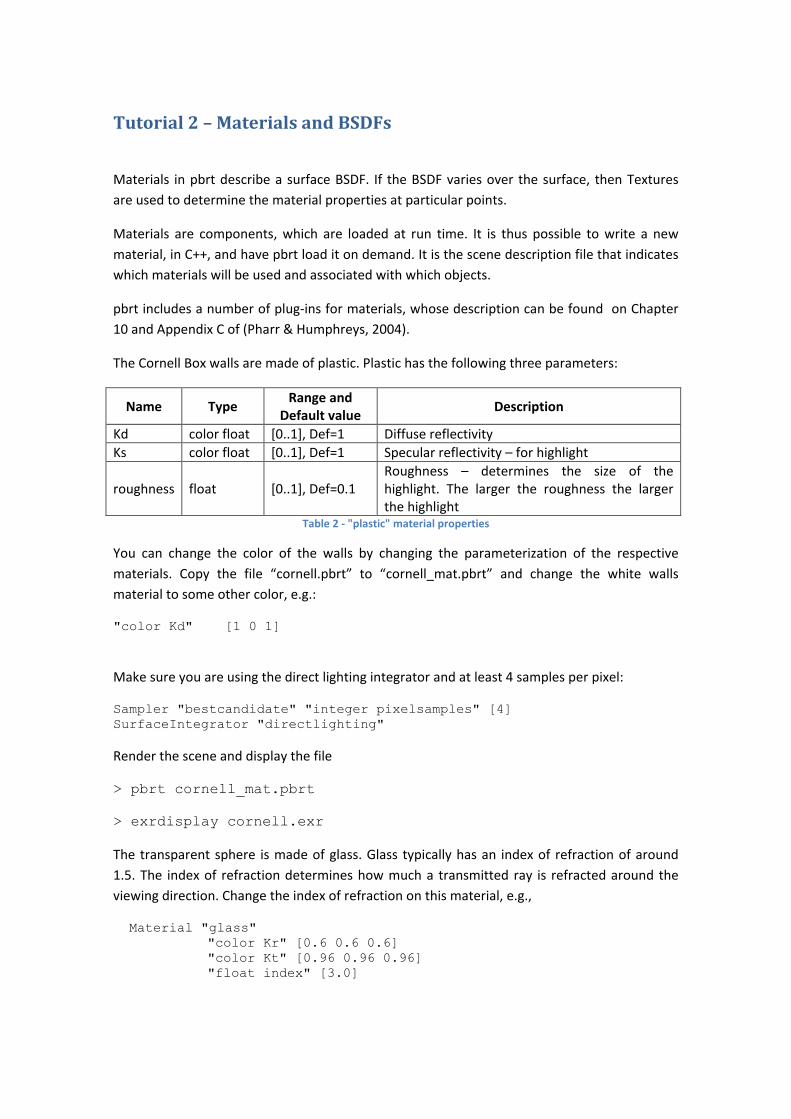
The Cornell Box walls are made of plastic. Plastic has the following three parameters:

Name Type Range and

Default value Description

Kd color float [0..1], Def=1 Diffuse reflectivity

Ks color float [0..1], Def=1 Specular reflectivity – for highlight

roughness float [0..1], Def=0.1

Roughness – determines the size of the

highlight. The larger the roughness the larger

the highlight Table 2 - "plastic" material properties

You can change the color of the walls by changing the parameterization of the respective

materials. Copy the file “cornell.pbrt” to “cornell_mat.pbrt” and change the white walls

material to some other color, e.g.:

"color Kd" [1 0 1]

Make sure you are using the direct lighting integrator and at least 4 samples per pixel:

Sampler "bestcandidate" "integer pixelsamples" [4] SurfaceIntegrator "directlighting"

Render the scene and display the file

> pbrt cornell_mat.pbrt

> exrdisplay cornell.exr

The transparent sphere is made of glass. Glass typically has an index of refraction of around

1.5. The index of refraction determines how much a transmitted ray is refracted around the

viewing direction. Change the index of refraction on this material, e.g.,

Material "glass" "color Kr" [0.6 0.6 0.6] "color Kt" [0.96 0.96 0.96] "float index" [3.0]

You can also change the color of the glass by changing the remaining parameters:

# glass material Material "glass" "color Kr" [0.6 0.6 0.6] "color Kt" [0 0.96 0] "float index" [3]

Textures

Textures are used to spatially vary the BRDF parameters. In pbrt you have to either create the

texture (if it is procedural) or load it (if it is an image map) and then associate the texture with

a material parameter.

Textures might either be maps of floats or “color” data type. The latter is a vector with as

many floats as the “Spectrum” data type; by default this is 3 elements: R, G and B. pbrt can

generate procedural textures; these are plug-ins, thus the set of procedural textures can be

increased by writing new components. The set of provided textures is described in page 931

of (Pharr & Humphreys, 2004).

Add the following line to cornell_mat.pbrt to create a checkerboard procedural texture,

named checks:

Texture "checks" "color" "checkerboard" "float uscale" [4] "float vscale" [4] "color tex1" [0 0 1] "color tex2" [0 1 1]

You can now associate this texture with parameters of any given material. For example,

change the white wall diffuse reflection coefficient:

Material "plastic" "texture Kd" "checks" "color Ks" [0.1 0.1 0.1] "float roughness" 0.15

Textures can also be loaded from a file in EXR format. The following line loads a float texture

from file textures/sponza/sp_luk.exr and names it sponza-bump:

Texture "sponza-bump" "float" "imagemap" "string filename" ["textures/sponza/sp_luk.exr"]

You can now modulate any one-dimensional parameter. It can also be used as a bump map, to

perturb a surface shading normal. The following command bump maps the white wall:

Material "plastic" "texture Kd" "checks" "color Ks" [0.1 0.1 0.1] "float roughness" 0.15 "texture bumpmap" "sponza-bump"

Play around with textures to modulate any material you want.

Tutorial 3

Introduction

During this tutorial you will write a pbrt Surface Integrator for Whitted

read carefully Appendix A to understand how to write plug

presented there. These surface integrators (flat, depth, DirectNoShadows) are distributed with

this tutorial.

We will build on the DirectNoSha

complexity to it.

Remember that this integrator does not shoot shadow rays. It uses the following expression to

shade each point:

DirectShadows integrator

The DirectShadows integrator evaluates the reflected radiance at the intersection point due to

direct lighting (

shoots shadow rays and thus object

given by

where

source s

In pbrt the

shoot this shadow feeler. This method is

the scene

unoccluded. Add this call to the DirectNoShadows, selecting carefully where to call this

method.

results obtained with 1 and 64 primary rays per pixel, with rendering times of 2 and 126.8

seconds, respectively.

Tutorial 3 –

Introduction




this tutorial.


complexity to it.


shade each point:



direct lighting (directly


given by � � ∑for all light sources i

where V(p,Li) stands for visibility between the intersection point

source surface. This function is evaluated by casting a ray and returns either 1 or 0.

In pbrt the LighT::Sample_L()


the scene as a parameter and returns a Boolean: true if the light source is visible, false if it is


method. REMEMBER



Whitted ray tracing surface integrator






shade each point:

� � �for all light sources i



directly from the light sources), but taking into consideration occlusions, i.e., it


for all light sources i

stands for visibility between the intersection point

urface. This function is evaluated by casting a ray and returns either 1 or 0.

LighT::Sample_L()


as a parameter and returns a Boolean: true if the light source is visible, false if it is


EMEMBER: shooting rays is the most expensive task in a ray tracer.







We will build on the DirectNoShadows Surface Integrator and will incrementally add


� ��ray directionfor all light sources i



from the light sources), but taking into consideration occlusions, i.e., it

shoots shadow rays and thus objects cast shadows onto each others. The returned radiance is

��ray directionfor all light sources i



LighT::Sample_L() method returns a visibility tester that can be used to




: shooting rays is the most expensive task in a ray tracer.






dows Surface Integrator and will incrementally add


�ray direction



s cast shadows onto each others. The returned radiance is

ray direction, ��



method returns a visibility tester that can be used to

shoot this shadow feeler. This method is VisibilityTester::Unoccluded()







read carefully Appendix A to understand how to write plug-ins and examine the examples




ray direction, �� cos




� � �� cos ��




VisibilityTester::Unoccluded()






During this tutorial you will write a pbrt Surface Integrator for Whitted style ray tracing. Please

ins and examine the examples




cos �� , !��"




�� , !��" � #�$,

stands for visibility between the intersection point p and a point at the i



VisibilityTester::Unoccluded()





style ray tracing. Please





"




, ��"

and a point at the ith



VisibilityTester::Unoccluded(). It takes



: shooting rays is the most expensive task in a ray tracer. Below are the


style ray tracing. Please








th light


. It takes



Below are the


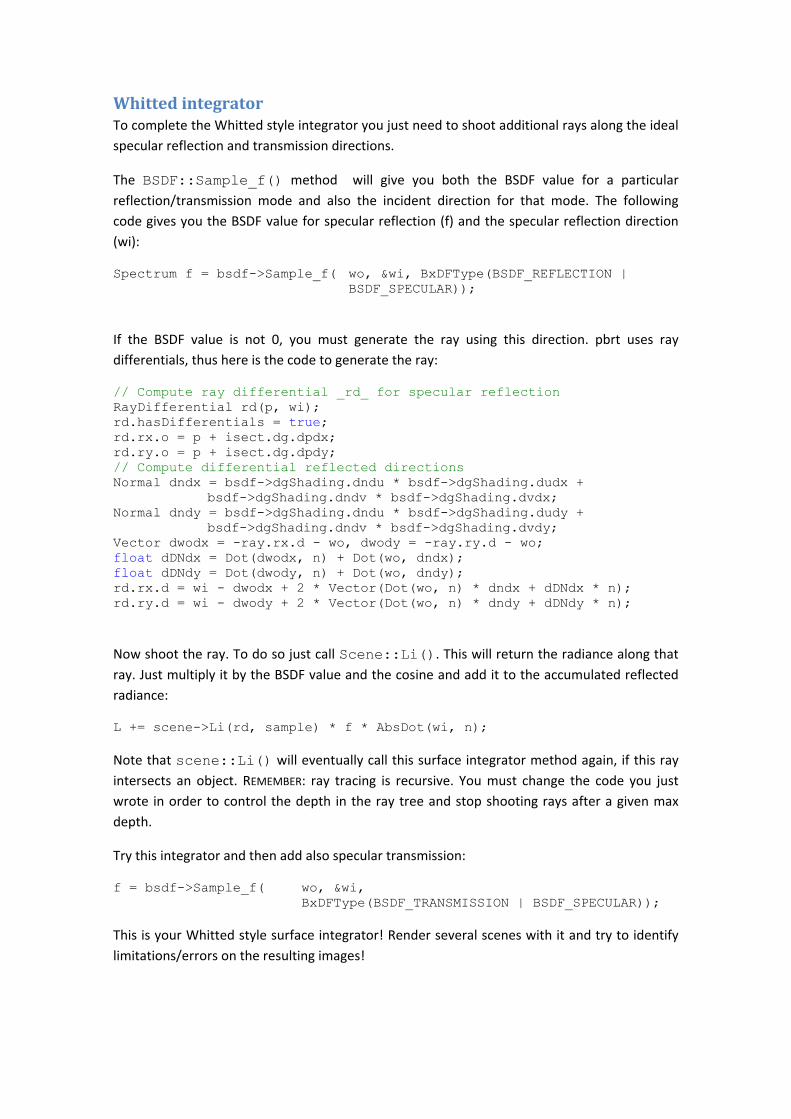
Whitted integrator

To complete the Whitted style integrator you just need to shoot additional rays along the ideal

specular reflection and transmission directions.

The BSDF::Sample_f() method will give you both the BSDF value for a particular

reflection/transmission mode and also the incident direction for that mode. The following

code gives you the BSDF value for specular reflection (f) and the specular reflection direction

(wi):

Spectrum f = bsdf->Sample_f( wo, &wi, BxDFType(BSDF_REFLECTION | BSDF_SPECULAR));

If the BSDF value is not 0, you must generate the ray using this direction. pbrt uses ray

differentials, thus here is the code to generate the ray:

// Compute ray differential _rd_ for specular reflection RayDifferential rd(p, wi); rd.hasDifferentials = true; rd.rx.o = p + isect.dg.dpdx; rd.ry.o = p + isect.dg.dpdy; // Compute differential reflected directions Normal dndx = bsdf->dgShading.dndu * bsdf->dgShading.dudx + bsdf->dgShading.dndv * bsdf->dgShading.dvdx; Normal dndy = bsdf->dgShading.dndu * bsdf->dgShading.dudy + bsdf->dgShading.dndv * bsdf->dgShading.dvdy; Vector dwodx = -ray.rx.d - wo, dwody = -ray.ry.d - wo; float dDNdx = Dot(dwodx, n) + Dot(wo, dndx); float dDNdy = Dot(dwody, n) + Dot(wo, dndy); rd.rx.d = wi - dwodx + 2 * Vector(Dot(wo, n) * dndx + dDNdx * n); rd.ry.d = wi - dwody + 2 * Vector(Dot(wo, n) * dndy + dDNdy * n);

Now shoot the ray. To do so just call Scene::Li(). This will return the radiance along that

ray. Just multiply it by the BSDF value and the cosine and add it to the accumulated reflected

radiance:

L += scene->Li(rd, sample) * f * AbsDot(wi, n);

Note that scene::Li() will eventually call this surface integrator method again, if this ray

intersects an object. REMEMBER: ray tracing is recursive. You must change the code you just

wrote in order to control the depth in the ray tree and stop shooting rays after a given max

depth.

Try this integrator and then add also specular transmission:

f = bsdf->Sample_f( wo, &wi, BxDFType(BSDF_TRANSMISSION | BSDF_SPECULAR));

This is your Whitted style surface integrator! Render several scenes with it and try to identify

limitations/errors on the resulting images!

NOTE:

This Whitted style integrator presents some noise in shadows. A completely deterministic

integrator should not present noise.

Noise appears because the method Lights::Sample_L() randomly selects the sample point over

the light source surface area. Does shadow rays are being shot towards different points on the

light sources and this is perceived as noise. There is another form of this method which allows

deterministic sampling of the light sources. Change the following line

Spectrum Li = scene->lights[i]->Sample_L(p, &wi, &visibility);

to

Spectrum Li = scene->lights[i]->Sample_L(p, 0.5, 0.5, &wi, &pdf,

&visibility);

Declare a float variable named pdf and also change

L += f * Li * AbsDot(wi, n);

to

L += f * Li / pdf * AbsDot(wi, n);

Now your Whitted style integrator is fully deterministic and the resulting image will present

aliasing (e.g., jagged edges in the shadows boundaries) rather than noise.

Tutorial 4 – Sampling the image plane and light sources

The efficiency (execution time) and amount of noise (variance) associated with a given

rendering algorithm depend on the sampling distribution and density used.

Throughout this tutorial you will try different sampling distributions and densities for both the

image plane and area light sources in order to get an insight on how these relate to execution

time and noise.

Open the cornell box file and make sure you are using Mitchell filter, the stratified sampler

with jittering on and the direct lighting surface integrator:

PixelFilter "mitchell" "float xwidth" [2] "float ywidth" [2]

SurfaceIntegrator "directlighting"

Sampler "stratified" "bool jitter" ["true"] "integer xsamples" [1] "integer

ysamples" [1]

The area of Mitchell filter is 4 and we are requesting one sample per pixel (spp) using a

stratified jittered distribution.

When you specify and area light you can also specify how many shadow rays should be shot to

sample that light source (although it is the surface integrator responsibility to respect this or

not – direct lighting does). The parameter nsamples indicates precisely this, i.e, samples per

light source (spl).

AreaLightSource "area"

"color L" [25 25 25]

"integer nsamples" [1]

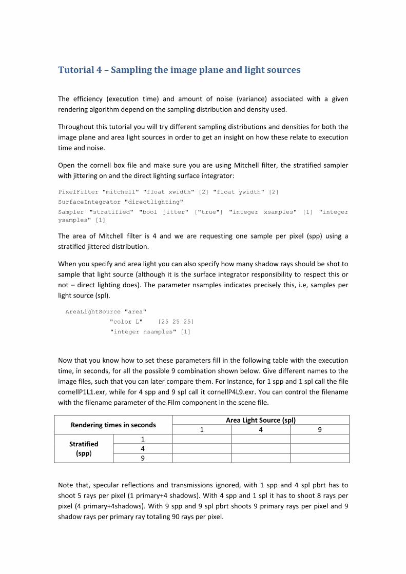
Now that you know how to set these parameters fill in the following table with the execution

time, in seconds, for all the possible 9 combination shown below. Give different names to the

image files, such that you can later compare them. For instance, for 1 spp and 1 spl call the file

cornellP1L1.exr, while for 4 spp and 9 spl call it cornellP4L9.exr. You can control the filename

with the filename parameter of the Film component in the scene file.

Rendering times in seconds Area Light Source (spl)

1 4 9

Stratified

(spp)

1

4

9

Note that, specular reflections and transmissions ignored, with 1 spp and 4 spl pbrt has to

shoot 5 rays per pixel (1 primary+4 shadows). With 4 spp and 1 spl it has to shoot 8 rays per

pixel (4 primary+4shadows). With 9 spp and 9 spl pbrt shoots 9 primary rays per pixel and 9

shadow rays per primary ray totaling 90 rays per pixel.

Comparing the subjective quality of the final images and the respective rendering times try to

answer these questions:

1. Which gives the best result: 1 spp x 9 spl or 9 spp x 1 spl? Why? Remember to compare

both the quality of the direct lighting (shadows) and the noise in the objects’ edges.

2. If you had to weight subjective image quality and objective execution time which

combination of spp x spl would you use? Why?

Recently sampling distributions based on quasi-random numbers sequences, rather than

pseudo-random sequences, have been used to sample multi dimensions of the rendring

problem. pbrt includes one such sampler: low discrepancy. Render an image with 4 spp and 1

spl using this sampler and compare both execution time and subjective quality with those

obtained with stratified jittering, by filling the table below (NOTE: the difference in subjective

quality might be more apparent if you use 16 spp and 1 spl – it takes a bit longer, though).

Indicate to pbrt core that it must use low discrepancy by selecting the appropriate sampler:

Sampler "lowdiscrepancy" "integer pixelsamples" [4]

Stratified Low discrepancy

Execution time (secs)

Subjective Quality

Which would you recommend?

Tutorial 5 – Monte Carlo Rendering

Download the code for the path tutorial integrator, add it as a new project to the pbrt Solution

and build the new integrator.

Study the code carefully. Notice that it first evaluates the ray intersection with the scene:

scene->Intersect(ray, &isect)

then evaluates direct lighting followed by indirect lighting.

Direct lighting is evaluated by sampling all light sources. A random position is selected on the

surface of each light source:

Spectrum Li = scene->lights[i]->Sample_L(p, &wi, &visibility);

and then this light contribution is added to the reflected radiance, if the light source is visible

from the shading point:

if (!f.Black() && visibility.Unoccluded(scene)) Lr += f * Li * AbsDot(wi, n);

Indirect lighting is then evaluated if the maximum length of the random walk has not been

reached (depth of the recursive algorithm). A random direction over the sphere is requested:

Spectrum f = bsdf->Sample_f(wo, &wi, BSDF_ALL, &flags);

The ray differential is built and a new ray is shot along this direction and added to the reflected

radiance:

depth++; Lr += scene->Li(rd, sample) * f * AbsDot(wi, n); depth--;

Change the cornell box scene description file to use this surface integrator and request a

single sample per pixel:


SurfaceIntegrator "path_tutorial"

Render the image, visualize it and write down the rendering time and number of shadow rays

traced. What are the causes of noise (variance) seen on this image?

Direct Lighting

This integrator is sampling all light sources for each intersection with the scene geometry (note

that the Cornell box has various light sources, since the lamp in the ceiling is described by

multiple triangle meshes, each representing a different light source).

In a scene with many light sources, evaluating them all for each point being shaded might not

be desirable, since this requires many shadow rays. What the integrator does is to add the

contributions of all the light sources to compute the total direct lighting. Each light source can

be seen as a different function, ��%", and we want to compute the expected value of the sum

of all these functions: &[∑ ��(")*�+, ], . being the number of light sources.

Monte Carlo integration allows us to avoid sampling all light sources. If we randomly select

one of them, with uniform probability $��" � ,)*

, then we can evaluate this single light source,

divide its contribution by the probability of selecting it (or multiply by the number of light

sources) and still get a correct result in average.

Change your code to do exactly this. Select the light source using:

int NumLights = scene->lights.size(); int l = Floor2Int(RandomFloat()* NumLights); l = min(l, NumLights-1);

and then do not forget to multiply its contribution by NumLights:

Lr += f * Li * AbsDot(wi, n) * ((float)NumLights);

Render the image, visualize it and compare it with the one from the previous section.

Comment the variance in the image, rendering time and number of shadow rays traced.

Additional Material

The previous exercise asked you to select a single light source with uniform probability,

$��" � ,)*

. This distribution does not use any information about the light sources total power

or position. Alternatively, a probability distribution might be built using information about

these quantities, does doing direct light importance sampling.

You can:

1. Build a probability distribution based on the light sources radiant power, with each

light source probability being $��" � !/012�34"∑ !/012�35"6*

578.

The power of each light source is given by pbrt:

Spectrum power = light->Power(scene);

2. A better distribution might be based on the solid angle subtended by each light source

when seen from p. This distribution, however, has to be build for each point p.

Remember that the solid angle is given by 9 � :; <=> ?;2@ .

Indirect Lighting

This path tracer always stops its random walk after a fixed number of intersections (parameter

maxdepth). This results in a biased estimation of the integral.

An unbiased alternative is to use Russian Roulette. An absorption (or termination) probability,

q, is given as a parameter. Before shooting a new secondary ray a random number in the

interval [0..1[ is taken. If this number is larger than q, then the secondary ray is shot; if it is less

it is not shot. The contribution of those rays that are shot must be weighted by a factor

1 �1 − C"⁄ to account for the rays that were not spawned.

Change this integrator such that it accepts a new float parameter, absorption. If this

parameter, whose default value should be 0, is different from 0, then Russian Roulette is used

instead of deterministic termination.

Render the cornell box for different values of q and compare both noise, rendering time and

number of triangle ray intersections.

To have a good idea about the rendering capabilities and computing power demands of path

tracing run a few images with different numbers of samples per pixel:


With path tracing the random walk at each intersection point continues along a single

direction. Alternatively, Monte Carlo ray tracing selects N directions at each intersection point.

The contribution of each of them is integrated using the Monte Carlo estimator:

��EF�$ → 92" ≈ 1 �1 − C" � �2�$, 92 , 9�"��EF�$ ← 9�" cos J�

$�9�")

�+,

Change your integrator such that it accepts a new integer parameter, split, which indicates

the split number at each intersection, i.e., the number of secondary rays to shoot at each

intersection. Its default value must be 1, corresponding to the path tracing case.

Render an image of the Cornell Box with split=2. Comment on noise and execution time.

Tutorial 6 – Irradiance Cache

The irradiance cache (IC) surface integrator distributed with pbrt does direct lighting using a

Monte Carlo integrator for all the light sources, follows specular transmission and reflection

paths by spawning a ray for each of these components and then evaluates indirect diffuse

lighting by using the irradiance cache. Cosine weighted importance sampling is used to sample

the hemisphere, although not stratified as suggested on Greg Ward’s original paper.

The integrator accepts the following main parameters:

Parameter Description Default

maxerror Maximum error estimate for

accepting a sample for interpolation

0.2

nsamples Number of directions (rays) used to

evaluate irradiance

4096

These parameters strongly influence both image quality and rendering time. In general,

smaller acceptable error results in more irradiance samples and, thus, larger execution time.

Increasing the number of directions to evaluate irradiance results in a better estimate of

irradiance, but also increases execution time. Remember, however, that this being a biased

method, increasing the number of samples does not guarantee a convergence to the correct

result.

Using the Cornell Box, fill the table below for the proposed different combinations of these

parameters. For each of them register execution time, number of irradiance estimates

(samples) computed and your own subjective ordering of image quality.

You can set the parameters by writing:

SurfaceIntegrator "irradiancecache" "integer nsamples" [512] "float maxerror" [0.2]

Make sure that only a single sample per pixel is taken:


maxerror

0.5 0.2 0.1

nsamples

512

2048

Sample Placement Visualization

Visualizing where, on 3D space, IC samples are placed helps in creating insight about how the

algorithm works with respect to the scene being rendered and what its requirements are.

Change the IC integrator such that whenever an IC sample has to be extensively calculated, the

corresponding pixel is set to a particular color (e.g black=(0.,0.,0.)).

SUGGESTION: locate the code sequence where IC values are evaluated and, if a sample is

evaluated, change the returned radiance value to the selected color. Make sure that the

sample is still evaluated and added to the cache, otherwise other pixels values will also be

affected.

Render the Cornell Box with the modified integrator and answer the following questions:

Q1.: Characterize the regions where samples tend to concentrate. What about those where

they tend to be more sparse?

Q2.: If you render the same scene with different values of the “nsamples” parameter, can you

notice any difference on the samples placement pattern? Why?

Q3.: If you render the same scene with different values of the “maxerror” parameter, can you

notice any difference on the samples placement pattern? Why?

Pre-process: cache warm-up

The Irradiance Cache algorithm suffers from a rendering order problem that results on many

visible artifacts on the final image.

The image is rendered in scanline order, one pixel at a time, starting from one corner,

processing that line and continuing to the next. Since the cache is initially empty, IC samples

end up being calculated in scanline order too; consequently, there are many extrapolations (a

single sample being used to estimate irradiance at another location) and there is never

information about irradiance on regions of the image that haven’t been processed yet. Many

of the artifacts you can see on the final image result from this problem.

A possible solution would be to do a first pass over the image plane, at a lower resolution

(sampling rate), and evaluate IC samples whenever required. These samples would be stored

on the cache and used on the second pass, done at full resolution. This pass would use samples

distributed all over the visible 3D volume, thus avoiding the extrapolations resulting from

scanline order IC calculation. Note that even if actual pixel values calculated on the first pass

are discarded and recomputed on the second pass, this will not, eventually, represent a

significant penalty since IC evaluation takes most of the rendering time.

Use the PreProcess() method to do this first pass at a lower resolution.

SUGGESTION: add a new parameter determining how many pixels (primary rays) should be

evaluated on this first pass. Its default value should be zero, resulting on a single pass

rendering.

Compare image quality, rendering time and number of IC samples evaluated between the two

pass approach and the single pass approach.

Tutorial 7 – Interactive Global Illumination

The interactive global illumination integrator performs a preprocess step, where particles

carrying radiant flux are propagated from the light sources into the scene. Whenever the path

of these light particles intersects geometry with a diffuse material a virtual point light source

(VPL) is created.

In rendering time all these VPLs are sampled with a shadow ray, contributing to the point

illumination if visible. Indirect diffuse lighting is thus included on the integral. The number of

light paths traced from the light sources is determined by the nlights integer parameter;

the number of VPLs is usually larger, since each light path can originate more than one VPL.

If the same set of VPLs is used for all pixels, then neighboring pixels are highly intercorrelated.

Different sets of VPLs, each with nlights light paths can be created. The set to use for each

pixel is determined stochastically, thus resulting in a noisier image, which is visually more

acceptable. The number of sets to generate is given by the nsets integer parameter.

Note that this approach does not increase rendering time, since the number of VPLs to sample

per pixel is the same as before. Preprocessing time will increase, since more VPLs have to be

generated. However, the number of VPLs is usually low, thus preprocessing time is a very small

fraction of total execution time.

An even better approach is to sample each pixel with several primary rays, thus reducing

aliasing, and use a different set of VPLs per primary ray. Each set can have a number of light

paths equal to the number of light paths we want to use per pixel divided by the number of

sets.

Using the Indirect Cornell Box scene, render it with a sample per pixel, 64 light samples and a

single set of VPLs:


SurfaceIntegrator "igi" "integer nlights" [64] "integer nsets" [1]

Now render it again but using 4 sets instead. Different pixels will use different sets of VPLs,

thus decreasing intercorrelation:



Compare the quality of both images and respective rendering time.

Render the image again, but using 4 samples per pixel. The number of VPLs samples per pixel

can be kept constant by reducing the number of VPLs per set (64/4=16):



Compare this image quality and rendering time with the previous one and justify why

rendering time has increased.

The igi surface integrator distributed with pbrt evaluates direct lighting in the usual way,

i.e., by sampling the light sources directly. A variation would be to consider the starting point

of each light path as a VPL too – note that these VPLs would be on the light source surface.

Instead of explicitly evaluating direct lighting, this would be evaluated by sampling these

additional VPLs.

Change the igi surface integrator to include this modification.

The PreProcess() method has to be changed to add the VPLs on the light sources surfaces

to each VPL set. The Li() method has to be changed, such that it no longer samples the light

sources directly – this will be done by evaluating the new VPLs.

Compare both image quality and rendering time.

Additional Material

The igi integrator randomly selects light sources from the whole set of light sources present

in the model (even if some importance sampling based on the lights relative radiant powers is

used).

In highly occluded environments most light sources do not contribute for the illumination of

visible objects. Consider for example a building with many rooms and many light sources per

room. If the observer is inside a room the vast majority of light sources on other rooms do not

contribute to this room illumination. Shooting VPLs from these other light sources and

sampling them in rendering time is thus a waste of computational power. Furthermore, since

the number of light paths is often less than the total number of light sources and since the

light sources where these light paths start are selected randomly, it may happen that no light

path start on the observer’s room and, thus, no VPLs are inside this room.

This problem can be alleviated if the light sources which are important for the current view

point are previously identified. If this can be done on a preprocessing stage, then all light

sources that do not contribute for the current view point can be given an importance equal to

zero, and won’t be selected as the starting point for the VPL propagation paths.

Note: for the method to be unbiased, it must be guaranteed that any light source that

contributes to the current view point is given an importance different from 0.

In [Wald, Benthin, Slusallek; “Interactive Global Illumination in Complex and Highly Occluded

Environments”; EG Symposium on Rendering, 2003] it is suggested that a low resolution pass

over the image plane is done using path tracing. By counting the number of hits each light

source gets from shadow rays, their relative importance can be computed. Note however that

this not guarantees that all important light sources are accounted for. To avoid bias a residual

importance can be assigned to all light sources, although this might result in starting light

paths from unimportant ones.

Change the PreProcess() method to implement this method and use it to render the

Indirect Cornell Box scene. Compare both image quality and rendering time with the original

igi integrator for the same parameterization.

Appendix A – Foundations for writing Surface Integrators plug-ins

Generic structure

Locating and identifying the plug-ins

pbrt looks for plug-ins at run time in the directories specified either by the environment

variable PBRT_SEARCHPATH or in the scene description file by the statement SearchPath.

Multiple directories might be specified by separating them by colons or semi-colons according

to the particular operating system syntax.

Which particular plug-ins to use for each scene, together with their parameters, is specified in

the description file, on the overall rendering options region. There is a default plug-in for each

type as well as their respective default values. The following scene description excerpt is an

example of how to specify the camera and pixel filter plug-ins and respective parameters. For

further details please see Appendix C of (Pharr & Humphreys, 2004).

Camera "perspective" "float fov" [30] PixelFilter "mitchell" "float xwidth" [2] "float ywidth" [2]

Table 3 - plug-ins specification in scene description

Methods

The C file defining a plug-in must contain the plug-in class and a method for its creation.This

method is entitled Create<Plug-In Type>() and receives as a parameter a ParamSet,

which will contain the plug-in parameters’ values as given on the scene description file. If the

parameters haven’t been specified on the description file, then this method will set their

default values. It then creates the object by allocating it. This method is called by the pbrt core,

upon loading the plug-ins.

The table below presents two examples of the creator method for a tone map operator and a

surface integrator.

Non Linear Tone Map Operator

extern "C" DLLEXPORT ToneMap *CreateToneMap(const ParamSet &ps) { float maxy = ps.FindOneFloat("maxY", 0.f); return new NonLinearOp(maxy); }

This operator has a single float parameter whose default value is 0.0

Surface Integrator

extern "C" DLLEXPORT SurfaceIntegrator *CreateSurfaceIntegrator(const ParamSet &params) { int maxDepth = params.FindOneInt("maxdepth", 5); return new ConstantIntegrator(maxDepth); }

This integrator has a single integer parameter whose default value is 5 Table 4 - Creation methods for plug-ins

The plug-in class must make available the object constructor and the particular plug-in

methods. Which methods each plug-in must implement depends on the plug-in class. A

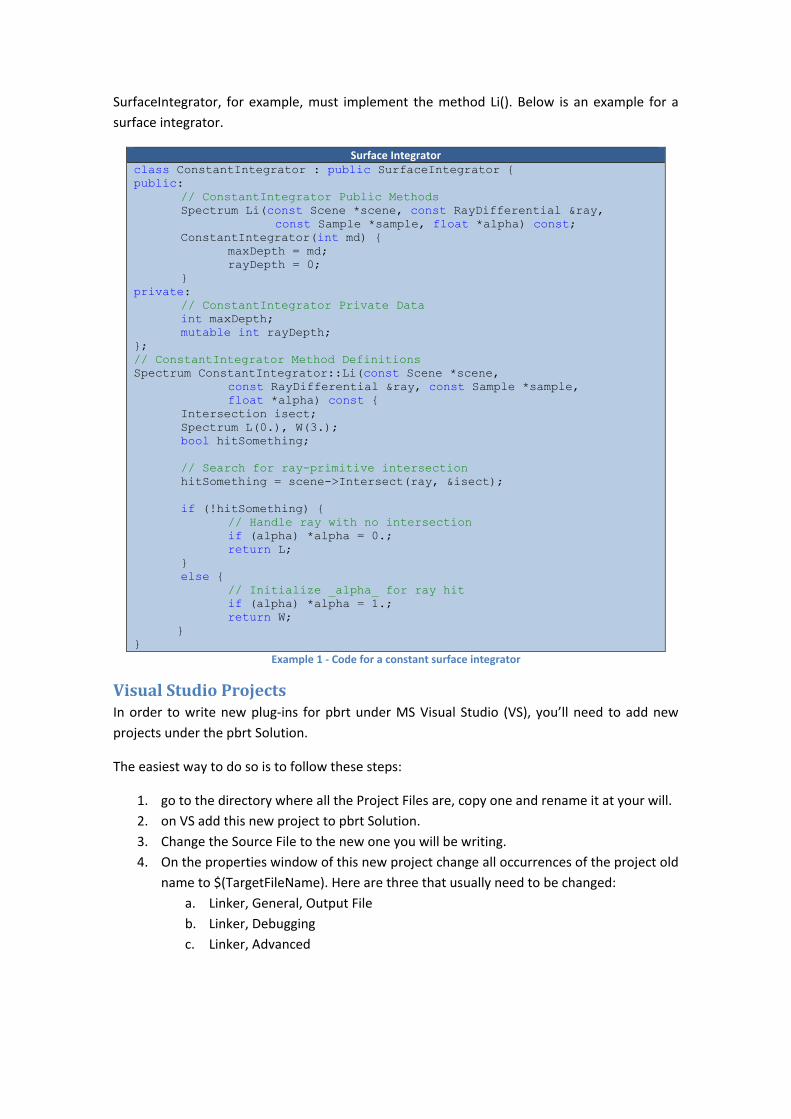
SurfaceIntegrator, for example, must implement the method Li(). Below is an example for a

surface integrator.

Surface Integrator

class ConstantIntegrator : public SurfaceIntegrator { public: // ConstantIntegrator Public Methods Spectrum Li(const Scene *scene, const RayDifferential &ray, const Sample *sample, float *alpha) const; ConstantIntegrator(int md) { maxDepth = md; rayDepth = 0; } private: // ConstantIntegrator Private Data int maxDepth; mutable int rayDepth; }; // ConstantIntegrator Method Definitions Spectrum ConstantIntegrator::Li(const Scene *scene, const RayDifferential &ray, const Sample *sample, float *alpha) const { Intersection isect; Spectrum L(0.), W(3.); bool hitSomething; // Search for ray-primitive intersection hitSomething = scene->Intersect(ray, &isect); if (!hitSomething) { // Handle ray with no intersection if (alpha) *alpha = 0.; return L; } else { // Initialize _alpha_ for ray hit if (alpha) *alpha = 1.; return W; } }

Example 1 - Code for a constant surface integrator

Visual Studio Projects

In order to write new plug-ins for pbrt under MS Visual Studio (VS), you’ll need to add new

projects under the pbrt Solution.

The easiest way to do so is to follow these steps:

1. go to the directory where all the Project Files are, copy one and rename it at your will.

2. on VS add this new project to pbrt Solution.

3. Change the Source File to the new one you will be writing.

4. On the properties window of this new project change all occurrences of the project old

name to $(TargetFileName). Here are three that usually need to be changed:

a. Linker, General, Output File

b. Linker, Debugging

c. Linker, Advanced

Surface Integrator Plug-Ins

Surface integrators compute radiance scattered from a surface along an outgoing direction.

They are responsible for evaluating the integral equation that describes the equilibrium

distribution of radiance in an environment – the rendering equation. The surface integral will

determine which light paths are traced through the environment.

The key method that every surface integrator must provide is Integrator::Li(). This method

receives as parameters the scene, a ray differential, a sample and a float, alpha, which is a

reference parameter used to return the value of alpha (0 for transparent .. 1 completely

opaque). It returns the spectral radiance along the given ray.

Spectrum Integrator::Li (const Scene *scene, const RayDifferential &ray, const Sample

*sample, float *alpha) const;

Table 5 - Integrator ::Li() signature method

Some methods and attributes from other classes are essential to write a surface integrator.

Below is a brief description of some of these.

// Search for ray-primitive intersection bool Scene::Intersect(const Ray &ray, Intersection *isect) const;

This method searches for an intersection between the given ray and the scene. It

returns a Boolean indicating whether some object is intersected. The Intersection

parameter will hold information regarding the intersection object and point.

• BSDF *isect.GetBSDF(Ray) – pointer to the BSDF at the intersection point

• Point isect.GetBSDF(Ray)->dgShading.p – intersection point

• Normal isect.GetBSDF(Ray)->dgShading.nn – normal at p

• Spectrum isect.GetBSDF(Ray)->f(wo, wi) – Value for the BSDF at the

intersection point for the incident (wi) and outgoing (wo) directions pair

• Spectrum isect.Le (-ray.d) – auto emitted radiance along ray direction

• float ray.maxt – intersection distance // Light sources

• int Scene::lights.size() – number of light sources

• Spectrum Light->Le(ray) – radiance emitted along the ray direction by

infinitely far away light sources that surround the entire scene

• Spectrum Light::Sample_L(const Point &p, Vector *wi, VisibilityTester *vis) const = 0;

This is the key method to evaluate radiance emitted by a particular light source

towards a particular point p. The caller passes the world space position of a point in

the scene and the light returns the radiance arriving at that point assuming there

are no object occluding them. The Light initializes the incident direction towards

the light source wi and the VisibilityTester which holds information about

the shadow ray that can be used to test whether the light is occluded. For area

lights a point on the light surface is stochastically selected. // Visibility Tester for light sources

• bool VisibilityTester:: Unoccluded (scene) – traces the shadow ray and

returns true if the light source is unoccluded Table 6 - Useful methods to write a surface integrator

Example: Depth integrator

The Depth integrator returns the depth of the intersection point p (distance to primary ray

origin):

This distance is given by

#include#include#include// Depth Declarationsclasspublic private };// Depth Method DefinitionsSpectrum Depth::Li( } externParamSet &params){ }



origin): � � KLMNOPQRThis distance is given by

#include "pbrt.h"#include "transport.h"#include "scene.h"// Depth Declarationsclass Depth : public:

// DepthSpectrum Li( Depth(}

private: // Depth Private Data

}; // Depth Method DefinitionsSpectrum Depth::Li(

Intersection isect;Spectrum L(0.);bool

// Search for rayhitSomething = scene

if (!hitSomething) { } else }

extern "C" DLLEXPORT SurfaceIntegrator *CreateSurfaceIntegrator(ParamSet &params)

return



KLMNOPQR �SOTThis distance is given by ray.maxt

"pbrt.h" "transport.h""scene.h"

// Depth Declarations Depth : public SurfaceIntegrator {

// Depth Public MethodsSpectrum Li(const

constDepth(void) {

// Depth Private Data

// Depth Method DefinitionsSpectrum Depth::Li(const

const RayDifferential &ray, float *alpha)

Intersection isect;Spectrum L(0.);

hitSomething;


(!hitSomething) {// Handle ray if (alpha) *alpha = 0.;return L;

{ // Initialize _alpha_ for ray hitif (alpha) *alpha = 1.;L = (ray.maxt, ray.maxt, ray.maxt);return L;

DLLEXPORT SurfaceIntegrator *CreateSurfaceIntegrator(ParamSet &params)

return new Depth();

Figure



SOT. VSLWLP, $"ray.maxt. The integrator returns 0 if no intersection is found.

Depth Surface Integrator

"transport.h"

SurfaceIntegrator {

Public Methods const Scene *scene, const Sample *sample,

// Depth Private Data

// Depth Method Definitions const Scene *scene,RayDifferential &ray, *alpha) const

Intersection isect; Spectrum L(0.);

hitSomething;

// Search for ray-primitive intersectionhitSomething = scene->Intersect(ray, &isect);

(!hitSomething) { // Handle ray with no intersection

(alpha) *alpha = 0.;L;

// Initialize _alpha_ for ray hit(alpha) *alpha = 1.;

L = (ray.maxt, ray.maxt, ray.maxt);L;

DLLEXPORT SurfaceIntegrator *CreateSurfaceIntegrator(

Depth();

Example 2 - Depth Surface Integrator code

Figure 1 - cornell box with depth integrator


"

. The integrator returns 0 if no intersection is found.


SurfaceIntegrator {

Scene *scene, constSample *sample,

Scene *scene, RayDifferential &ray, const

const {

primitive intersection>Intersect(ray, &isect);

with no intersection(alpha) *alpha = 0.;


L = (ray.maxt, ray.maxt, ray.maxt);


Depth Surface Integrator code

cornell box with depth integrator




const RayDifferential &ray,Sample *sample, float *alpha)

const Sample *sample,

primitive intersection >Intersect(ray, &isect);

with no intersection

// Initialize _alpha_ for ray hit

L = (ray.maxt, ray.maxt, ray.maxt);



cornell box with depth integrator (T=0.5 secs)



RayDifferential &ray,*alpha) const;

Sample *sample,

>Intersect(ray, &isect);



(T=0.5 secs)



RayDifferential &ray, ;

Sample *sample,

DLLEXPORT SurfaceIntegrator *CreateSurfaceIntegrator(const


Example:

The Flat integrator returns the

normal of the intersected surface at the intersection point p:

This does not depend on the light sources. For perfect diffuse surfaces the returned radiance

will be different from zero for all possible ray directions; for perfect specular surfaces the

returned radiance will only be different from zero if the ray direction is coincident with the

normal.

Spectrum Flat::Li( point }

Example: Flat integrator




be different from zero for all possible ray directions; for perfect specular surfaces the


normal.

Spectrum Flat::Li( Intersection isect;Spectrum L(0.), W(3.);bool


if (!hitSomething) { } else

point }

Flat integrator






Spectrum Flat::Li(constconst RayDifferential &ray, float *alpha)

Intersection isect;Spectrum L(0.), W(3.);

hitSomething;


(!hitSomething) {// Handle ray with no intersectionif (alpha) *alpha = 0.;return L;

{ // Initialize _alpha_ for ray hitif (alpha) *alpha = 1.;// Compute emitted and reflected light at ray intersection

// Evaluate BSDF at hit pointBSDF *bsdf = isect.GetBSDF(ray);// Initialize common variables for Whitted integratorconst Point &p = bsdfconst Normal &n = bsdfVector wo = Vector wi; // Compute emitted light if ray hit an area light sourceL += isect.Le(wo);wi = Vector (// get bsdf for this pair of directionsSpectrum f = bsdfL += f; return L;

Figure

The Flat integrator returns the BSDF for the pair of directions given by the primary ray and the





Flat Surface Integrator

const Scene *scene,RayDifferential &ray, *alpha) const

Intersection isect; Spectrum L(0.), W(3.);

hitSomething;

// Search for ray-primitive intersectionhitSomething = scene->Intersect(ray, &isect);

(!hitSomething) { // Handle ray with no intersection

(alpha) *alpha = 0.;L;


// Compute emitted and reflected light at ray intersection

// Evaluate BSDF at hit point*bsdf = isect.GetBSDF(ray);

// Initialize common variables for Whitted integratorPoint &p = bsdfNormal &n = bsdf

Vector wo = -ray.d; i; // incident direction

// Compute emitted light if ray hit an area light sourceL += isect.Le(wo); wi = Vector (-n); // get bsdf for this pair of directionsSpectrum f = bsdf->f(wo, wi);

L;

Example 3 - Flat Surface Integrator code

Figure 2 - cornell box with flat integrator (T=0.8 secs)

BSDF for the pair of directions given by the primary ray and the






Scene *scene, RayDifferential &ray, const

const {

primitive intersection>Intersect(ray, &isect);

// Handle ray with no intersection(alpha) *alpha = 0.;



// Evaluate BSDF at hit point*bsdf = isect.GetBSDF(ray);

// Initialize common variables for Whitted integratorPoint &p = bsdf->dgShading.p; Normal &n = bsdf->dgShading.nn;

ray.d; // outgoing direction // incident direction

// Compute emitted light if ray hit an area light source

// get bsdf for this pair of directions>f(wo, wi);

Flat Surface Integrator code

cornell box with flat integrator (T=0.8 secs)


normal of the intersected surface at the intersection point p: � �





const Sample *sample,

primitive intersection >Intersect(ray, &isect);

// Handle ray with no intersection

// Initialize _alpha_ for ray hit


// Evaluate BSDF at hit point *bsdf = isect.GetBSDF(ray);

// Initialize common variables for Whitted integrator>dgShading.p; // intersection point>dgShading.nn; // normal at p// outgoing direction

// incident direction // Compute emitted light if ray hit an area light source

// get bsdf for this pair of directions>f(wo, wi);

Flat Surface Integrator code



� ��−ray.direction




Sample *sample,

>Intersect(ray, &isect);


// Initialize common variables for Whitted integrator// intersection point// normal at p

// outgoing direction


// get bsdf for this pair of directions



direction, ��!"




Sample *sample,


// Initialize common variables for Whitted integrator // intersection point // normal at p







Example: DirectNoShadows integrator

The DirectNoShadows integrator evaluates the reflected radiance at the intersection point due

to direct lighting (directly from the light sources) without taking into consideration occlusions,

i.e., it does not shoot shadow rays. The returned radiance is given by

� � � ��ray direction, �� cos ��for all light sources i

, !��"

DirectNoShadows Surface Integrator

Spectrum directNoShadows::Li(const Scene *scene, const RayDifferential &ray, const Sample *sample, float *alpha) const { Intersection isect; Spectrum L(0.); bool hitSomething; // Search for ray-primitive intersection hitSomething = scene->Intersect(ray, &isect); if (!hitSomething) { // Handle ray with no intersection if (alpha) *alpha = 0.; // account for infinitely far away light sources for (u_int i = 0; i < scene->lights.size(); ++i) L += scene->lights[i]->Le(ray); if (alpha && !L.Black()) *alpha = 1.; return L; } else { // Initialize _alpha_ for ray hit if (alpha) *alpha = 1.; // Compute emitted and reflected light at ray intersection point // Evaluate BSDF at hit point BSDF *bsdf = isect.GetBSDF(ray); // Get the intersection point and the surface normal there const Point &p = bsdf->dgShading.p; // intersection point const Normal &n = bsdf->dgShading.nn; // normal at p Vector wo = -ray.d; // outgoing direction // Compute emitted light if ray hit an area light source L += isect.Le(wo); Vector wi; // incident direction // Add contribution of each light source for (u_int i = 0; i < scene->lights.size(); ++i) { VisibilityTester visibility; // Light::Sample_L() will return the incident radiance alog wi due to this particular light source // it does not check for visibility, but returns a VisibilityTester object that can later be used to do so Spectrum Li = scene->lights[i]->Sample_L(p, &wi, &visibility); if (Li.Black()) continue; // get bsdf for this pair of directions Spectrum f = bsdf->f(wo, wi); // if bsdf != 0 if (!f.Black()) // bsdf * Li * cos(wi, n) L += f * Li * AbsDot(wi, n); } return L; } }

Example 4 - DirectNoShadows surface integrator code

This surface integrator calls Light::Sample_L() to get the incident radiance at the

intersection point, p, coming directly from the light source. This method stochastically selects

a point in the surface of area light sources and returns both the direction from

and a visibility tester method that might be used to test if the light source is visible from

The image resulting from applying this integrator is full of noise. This occurs because the point

on the light sources surfaces is selected stochastically and will thus vary from intersection

point

methods.

There are several different ways to either reduce or eliminate variance. One approach is to

always select the same point on the area light source, thus the sampling b

deterministic and variance goes away. However, determinism has several problems, such as

aliasing, and is not a good solution. Another alternative is to shoot several primary rays per

pixel and then integrate their contribution. However, variance is

square root of the number of samples. This means that in order to halve variance, four times

more samples, i.e., primary rays, have to be evaluated. Unfortunately, rendering time is linear

with the number of primary rays

6.5, 25.7 and 104 seconds rendering time, respectively.



Figure



point to intersection

methods.












Figure 3 - cornell box with direct



intersection point. This noise is the visible effect of the variance inherent to stochastic












cornell box with direct



This noise is the visible effect of the variance inherent to stochastic








with the number of primary rays – see the images below with 4, 16 and 64 rays per pixel and




cornell box with direct no shadows integrator (1 rpp, T=1.2 secs)











the images below with 4, 16 and 64 rays per pixel and




no shadows integrator (1 rpp, T=1.2 secs)























pixel and then integrate their contribution. However, variance is inversely proportional to the




a point in the surface of area light sources and returns both the direction from p to this point

and a visibility tester method that might be used to test if the light source is visible from p






always select the same point on the area light source, thus the sampling becomes



inversely proportional to the




to this point

p.





ecomes



inversely proportional to the




Bibliographic References

Pharr, M., & Humphreys, G. (2004). Physically Based Rendering: from Theory to

Implementation. Morgan Kaufmann.

pbrt : a Tutorial - Universidade do Minhogec.di.uminho.pt/DISCIP/MInf/IFR0910/pbrtTutorials.pdf · pbrt : a Tutorial Luís Paulo Santos Departamento de Informática Universidade do

Documents