Pattern formation controlled by time-delayed feedback in bistable media

arX

iv:1

004.

2580

v2 [

nlin

.PS]

18

Sep

2010

jcp

Pattern formation controlled by time-delayed feedback in bistable

media

Ya-feng He1,2,∗ Bao-quan Ai1,3, and Bambi Hu1,4

1Centre for Nonlinear Studies, The Beijing-Hong Kong-Singapore

Joint Centre for Nonlinear and Complex Systems (Hong Kong),

Hong Kong Baptist University, Kowloon Tong, Hong Kong, China

2College of Physics Science and Technology,

Hebei University, Baoding 071002, China

3Laboratory of Quantum Information Technology, ICMP and SPTE,

South China Normal University, Guangzhou 510006, China

4Department of Physics, University of Houston, Houston, TX 77204-5005, USA.

(Dated: September 21, 2010)

Abstract

Effects of time-delayed feedback on pattern formation are studied both numerically and theo-

retically in a bistable reaction-diffusion model. The time-delayed feedback applied to the activator

and/or the inhibitor alters the behavior of the Nonequilibrium Ising-Bloch (NIB) bifurcation. If

the intensities of the feedbacks applied to the two species are identical, only the velocities of Bloch

fronts are changed. If the intensities are different, both the critical point of the NIB bifurcation

and the threshold of stability of front to transverse perturbations are changed. The effect of time-

delayed feedback on the activator opposes the effect of time-delayed feedback on the inhibitor.

When the time-delayed feedback is applied individually to one of the species, positive and nega-

tive feedbacks make the bifurcation point shift to different directions. The time-delayed feedback

provides a flexible way to control the NIB bifurcation and the pattern formation.

1

I. INTRODUCTION

Pattern formation has been of great interest in a variety of chemical, physical, and biolog-

ical contexts.1–5 A chemical front (interface) which connects two different states of system,

such as the excited and recovery states in excitable media, or the two stable states in

bistable media, plays an essential role on the pattern formation. Many literatures focus on

the dynamics of the front.6–15 Of particular interest is the front controlled by Nonequilib-

rium Ising-Bloch (NIB) bifurcation in the bistable media. The NIB bifurcation describes

a pitchfork bifurcation at which a stationary Ising front becomes unstable and a couple of

counterpropagating Bloch fronts appear. In bistable Ferrocyanide-Iodate-Sulfite reactions,

spirals, oscillating spots, and labyrinthine patterns have been observed.15–18 The spirals occur

in the Bloch region beyond the Nonequilibrium Ising-Bloch bifurcation. As a sparse spiral,

it results from an axisymmetry breaking of a shrinking ring. The oscillating spots appear

near but before the NIB bifurcation. The labyrinthine pattern originates from transverse

instability of a chemical front in Ising region. Similar patterns were also observed by Szalai

and De Kepper.17 These patterns observed in bistable Ferrocyanide-Iodate-Sulfite reactions

can be explained successfully in terms of a NIB bifurcation in a generic FitzHugh-Nagumo

model.8,19,20

Controlling the pattern formation is an important issue for the study of self-organization

phenomena far away from thermodynamic equilibrium. Recently, time-delayed feedback,

firstly presented by Ott et al to control the chaotic behavior of a deterministic system,21 has

been used to control the pattern formation successfully. It can control the tip trajectories

of spirals in a light-sensitive Belousov-Zhabotinsky reaction.22 A global feedback can either

stabilize the rigid rotation of a spiral or completely destroy spiral and suppress self-sustained

activity in a confined domain of excitable medium.23 The spontaneous suppression of spiral

turbulence based on feedback has been studied experimentally in a light-sensitive Belousov-

Zhabotinsky reaction and numerically in a modified FitzHugh-Nagumo model.24 With the

global feedback one can manipulate the competition between patterns with different sym-

metries (hexagons and rolls).25 In a delayed optical system, resonant Hopf triads lead to

drifting rhombic and hexagonal patterns.26 Near the codimension-two bifurcation points,

the time delay can result in a transition between Turing and Hopf instabilities.27,28

Most of the studies of the effects of time-delayed feedback on the pattern formation focus

2

on the dynamics of patterns in excitable and oscillatory media.22–24,27–33 How about the

effects of time-delayed feedback on controlling pattern formation in bistable media? In this

work, we study the role of time-delayed feedback played on controlling the NIB bifurcation

in a bistable FitzHugh-Nagumo model. We focus on the investigation of the NIB bifurcation

and the transverse instability of front when applying time delay. The underlying mechanism

of successful control is analyzed.

II. BISTABLE MODEL

The bistable media are described by a FitzHugh-Nagumo model:

ut = u− u3 − v +∇2u+ F, (1)

vt = ε(u− a1v − a0) + δ∇2v +G, (2)

where the time delay is applied with the forms:

F = gu(u(t− τ)− u(t)), (3)

G = gv(v(t− τ)− v(t)), (4)

here, the variables u and v represent the concentrations of the activator and inhibitor,

respectively, and δ denotes the ratio of their diffusion coefficients. τ indicates the delayed

time. gu and gv are the feedback intensities of variable u and v, respectively. The small

value ε characterizes the time scales of the two variables, where v remains approximately

constant vf on the length scale over which u varies. The system described by Eqs.(1) and

(2) can be either of excitable, Turing-Hopf, or bistable type. In this paper the parameter a1

is chosen such that the system is bistable. The two stationary and uniform stable states are

indicated by an up state (u+,v+) and a down state (u−,v−), respectively. The parameter a0

represents the symmetry of the system. In the following, we only consider the case that the

system is symmetric, i.e. a0=0, (u+,v+)=-(u−,v−). A front connects the two stable states

smoothly. It can be either traveling (Bloch front) or stationary (Ising) which is determined

by the control parameters.

Because pattern formations in bistable media are sensitive to the initial and boundary

conditions, we adopt fixed initial conditions during the numerical simulations. In the one-

dimensional case (200 grids, using Euler method), we focus on the traveling wave with an

3

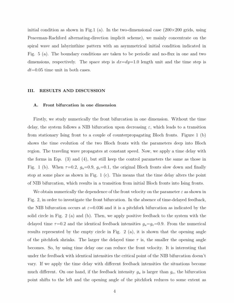
initial condition as shown in Fig.1 (a). In the two-dimensional case (200×200 grids, using

Peaceman-Rachford alternating-direction implicit scheme), we mainly concentrate on the

spiral wave and labyrinthine pattern with an asymmetrical initial condition indicated in

Fig. 5 (a). The boundary conditions are taken to be periodic and no-flux in one and two

dimensions, respectively. The space step is dx=dy=1.0 length unit and the time step is

dt=0.05 time unit in both cases.

III. RESULTS AND DISCUSSION

A. Front bifurcation in one dimension

Firstly, we study numerically the front bifurcation in one dimension. Without the time

delay, the system follows a NIB bifurcation upon decreasing ε, which leads to a transition

from stationary Ising front to a couple of counterpropagating Bloch fronts. Figure 1 (b)

shows the time evolution of the two Bloch fronts with the parameters deep into Bloch

region. The traveling wave propagates at constant speed. Now, we apply a time delay with

the forms in Eqs. (3) and (4), but still keep the control parameters the same as those in

Fig. 1 (b). When τ=0.2, gu=0.9, gv=0.1, the original Bloch fronts slow down and finally

stop at some place as shown in Fig. 1 (c). This means that the time delay alters the point

of NIB bifurcation, which results in a transition from initial Bloch fronts into Ising fronts.

We obtain numerically the dependence of the front velocity on the parameter ε as shown in

Fig. 2, in order to investigate the front bifurcation. In the absence of time-delayed feedback,

the NIB bifurcation occurs at ε=0.036 and it is a pitchfork bifurcation as indicated by the

solid circle in Fig. 2 (a) and (b). Then, we apply positive feedback to the system with the

delayed time τ=0.2 and the identical feedback intensities gu=gv=0.9. From the numerical

results represented by the empty circle in Fig. 2 (a), it is shown that the opening angle

of the pitchfork shrinks. The larger the delayed time τ is, the smaller the opening angle

becomes. So, by using time delay one can reduce the front velocity. It is interesting that

under the feedback with identical intensities the critical point of the NIB bifurcation doesn’t

vary. If we apply the time delay with different feedback intensities the situations become

much different. On one hand, if the feedback intensity gu is larger than gv, the bifurcation

point shifts to the left and the opening angle of the pitchfork reduces to some extent as

4

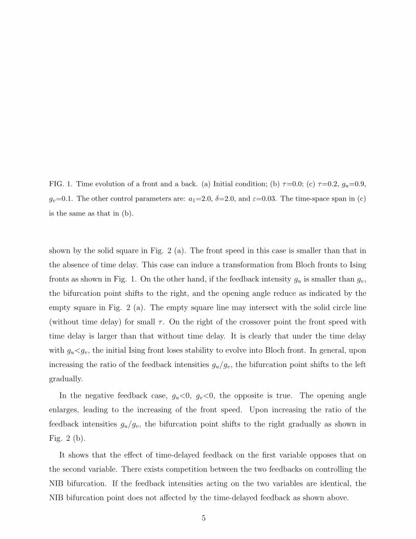
FIG. 1. Time evolution of a front and a back. (a) Initial condition; (b) τ=0.0; (c) τ=0.2, gu=0.9,

gv=0.1. The other control parameters are: a1=2.0, δ=2.0, and ε=0.03. The time-space span in (c)

is the same as that in (b).

shown by the solid square in Fig. 2 (a). The front speed in this case is smaller than that in

the absence of time delay. This case can induce a transformation from Bloch fronts to Ising

fronts as shown in Fig. 1. On the other hand, if the feedback intensity gu is smaller than gv,

the bifurcation point shifts to the right, and the opening angle reduce as indicated by the

empty square in Fig. 2 (a). The empty square line may intersect with the solid circle line

(without time delay) for small τ . On the right of the crossover point the front speed with

time delay is larger than that without time delay. It is clearly that under the time delay

with gu<gv, the initial Ising front loses stability to evolve into Bloch front. In general, upon

increasing the ratio of the feedback intensities gu/gv, the bifurcation point shifts to the left

gradually.

In the negative feedback case, gu<0, gv<0, the opposite is true. The opening angle

enlarges, leading to the increasing of the front speed. Upon increasing the ratio of the

feedback intensities gu/gv, the bifurcation point shifts to the right gradually as shown in

Fig. 2 (b).

It shows that the effect of time-delayed feedback on the first variable opposes that on

the second variable. There exists competition between the two feedbacks on controlling the

NIB bifurcation. If the feedback intensities acting on the two variables are identical, the

NIB bifurcation point does not affected by the time-delayed feedback as shown above.

5

0.00 0.02 0.04 0.06-0.90

-0.45

0.00

0.45

0.90

0.00 0.02 0.04 0.06-1.0

-0.5

0.0

0.5

1.0

c

(a)

(b)

c

FIG. 2. Dependence of the front velocity on the parameter ε. (a) Positive feedback, solid circle:

τ=0.0; empty circle: τ=0.2, gu=0.9, gv=0.9; solid square: τ=0.2, gu=0.9, gv=0.1; empty square :

τ=0.2, gu=0.1, gv=0.9. (b) Negative feedback, solid circle: τ=0.0; empty circle: τ=0.2, gu=−0.9,

gv=−0.9; solid square: τ=0.2, gu=−0.9, gv=−0.1; empty square : τ=0.2, gu=−0.1, gv=−0.9. The

other parameters are: δ=2.0, and a1=2.0.

If the feedback is applied individually, such that gu=0, or gv=0, we can still realize the

shift of the critical point of NIB bifurcation. Increasing the feedback gu (gv=0), for instance

from negative to positive values, the bifurcation point shifts from right to left gradually.

On the contrary, if increasing the feedback gv (gu=0) from negative to positive values, the

bifurcation point shifts from left to right. It shows that the effect of the time delay with

positive feedback on the variables opposes the effect of time delay with negative feedback

on the variables. Therefore, by using time delay with appropriate forms one can control the

front bifurcation efficiently.

In the absence of the time-delayed feedback the front bifurcation in one dimension is

determined by the relation between the front velocity and the parameter ε,9,20

6

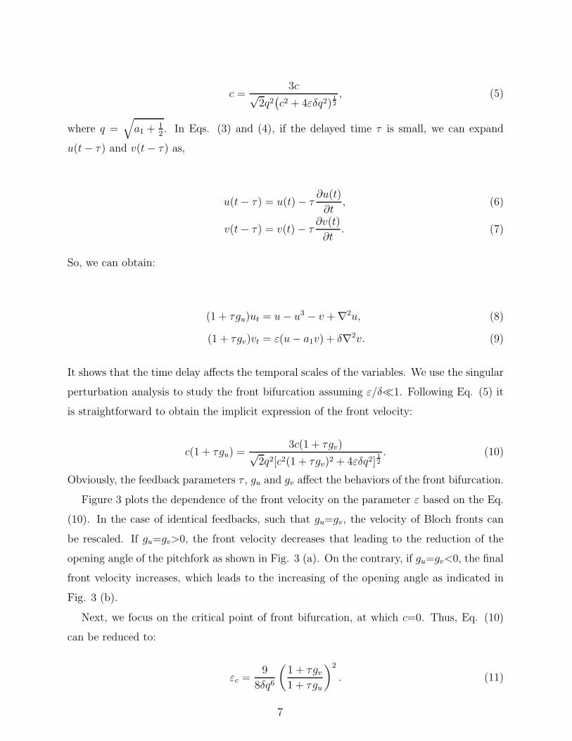
c =3c√

2q2(

c2 + 4εδq2)1

2

, (5)

where q =√

a1 +1

2. In Eqs. (3) and (4), if the delayed time τ is small, we can expand

u(t− τ) and v(t− τ) as,

u(t− τ) = u(t)− τ∂u(t)

∂t, (6)

v(t− τ) = v(t)− τ∂v(t)

∂t. (7)

So, we can obtain:

(1 + τgu)ut = u− u3 − v +∇2u, (8)

(1 + τgv)vt = ε(u− a1v) + δ∇2v. (9)

It shows that the time delay affects the temporal scales of the variables. We use the singular

perturbation analysis to study the front bifurcation assuming ε/δ≪1. Following Eq. (5) it

is straightforward to obtain the implicit expression of the front velocity:

c(1 + τgu) =3c(1 + τgv)√

2q2[c2(1 + τgv)2 + 4εδq2]1

2

. (10)

Obviously, the feedback parameters τ , gu and gv affect the behaviors of the front bifurcation.

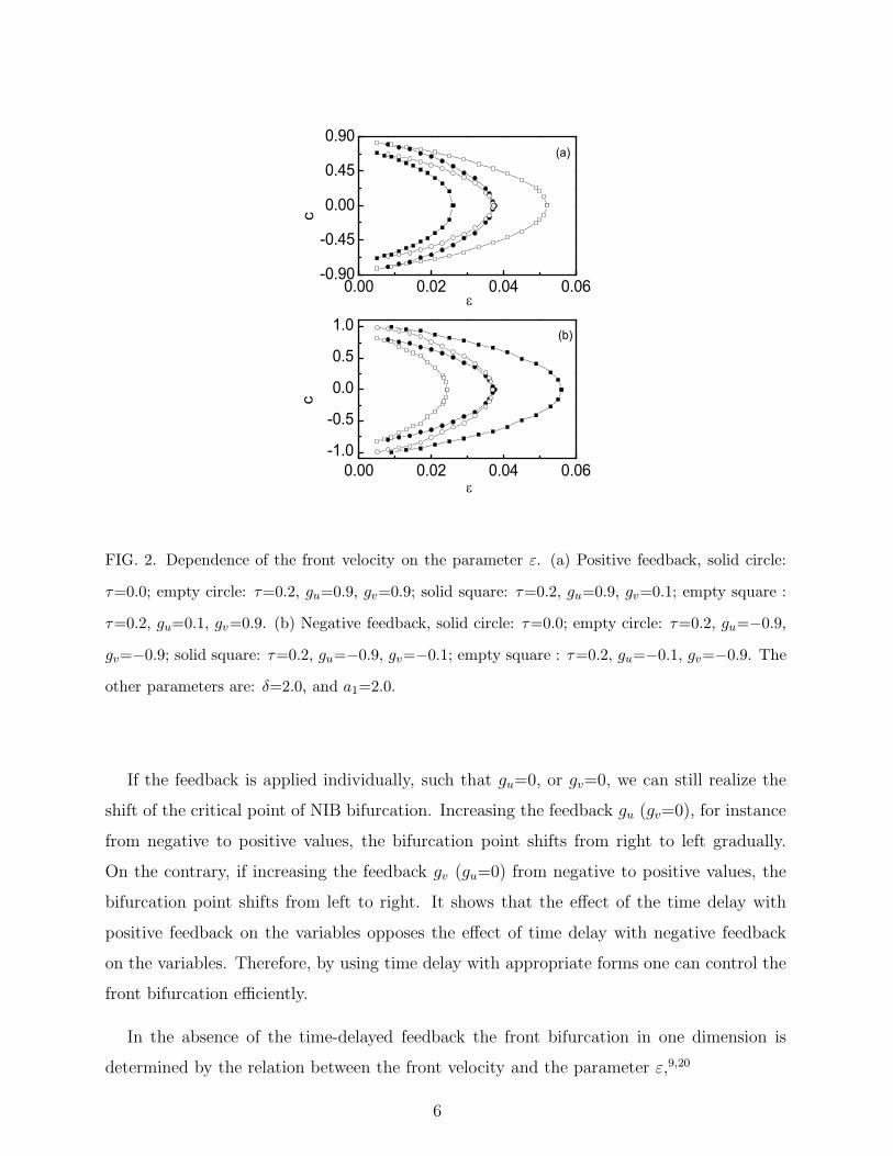
Figure 3 plots the dependence of the front velocity on the parameter ε based on the Eq.

(10). In the case of identical feedbacks, such that gu=gv, the velocity of Bloch fronts can

be rescaled. If gu=gv>0, the front velocity decreases that leading to the reduction of the

opening angle of the pitchfork as shown in Fig. 3 (a). On the contrary, if gu=gv<0, the final

front velocity increases, which leads to the increasing of the opening angle as indicated in

Fig. 3 (b).

Next, we focus on the critical point of front bifurcation, at which c=0. Thus, Eq. (10)

can be reduced to:

εc =9

8δq6

(

1 + τgv1 + τgu

)2

. (11)

7

0.00 0.02 0.04 0.06-0.90

-0.45

0.00

0.45

0.90

0.00 0.02 0.04 0.06-1.0

-0.5

0.0

0.5

1.0

(a)

c

c0

(b)c

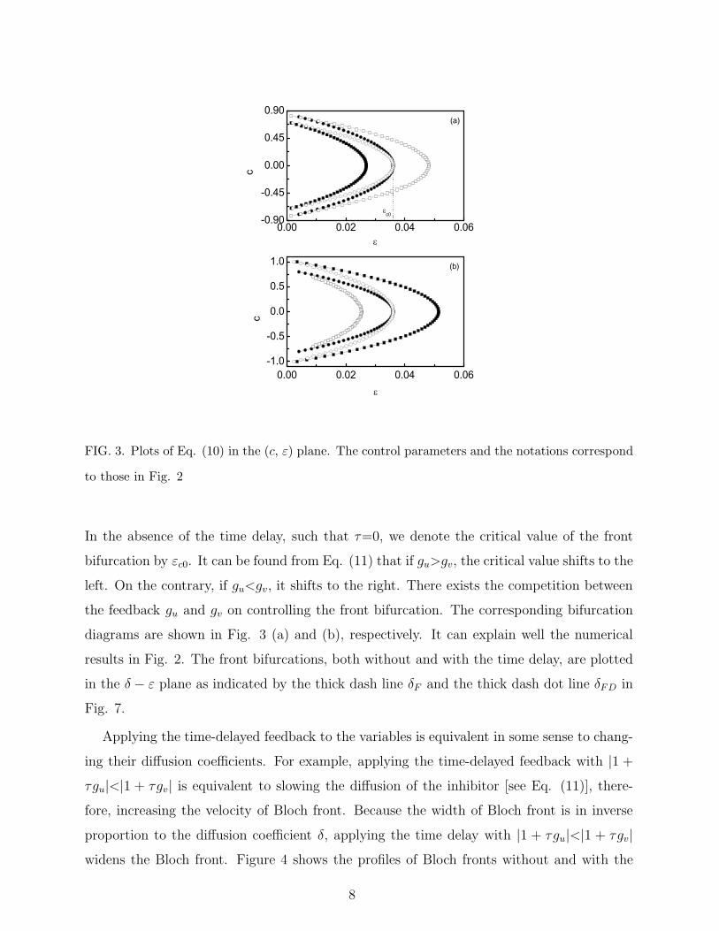
FIG. 3. Plots of Eq. (10) in the (c, ε) plane. The control parameters and the notations correspond

to those in Fig. 2

In the absence of the time delay, such that τ=0, we denote the critical value of the front

bifurcation by εc0. It can be found from Eq. (11) that if gu>gv, the critical value shifts to the

left. On the contrary, if gu<gv, it shifts to the right. There exists the competition between

the feedback gu and gv on controlling the front bifurcation. The corresponding bifurcation

diagrams are shown in Fig. 3 (a) and (b), respectively. It can explain well the numerical

results in Fig. 2. The front bifurcations, both without and with the time delay, are plotted

in the δ − ε plane as indicated by the thick dash line δF and the thick dash dot line δFD in

Fig. 7.

Applying the time-delayed feedback to the variables is equivalent in some sense to chang-

ing their diffusion coefficients. For example, applying the time-delayed feedback with |1 +τgu|<|1 + τgv| is equivalent to slowing the diffusion of the inhibitor [see Eq. (11)], there-

fore, increasing the velocity of Bloch front. Because the width of Bloch front is in inverse

proportion to the diffusion coefficient δ, applying the time delay with |1 + τgu|<|1 + τgv|widens the Bloch front. Figure 4 shows the profiles of Bloch fronts without and with the

8

-1

0

1

0 50 100 150 200-1

0

1

1

=0.0

vu

L1

(b)

(a)

u,v

2

=0.2

uv

L2 u,v

x

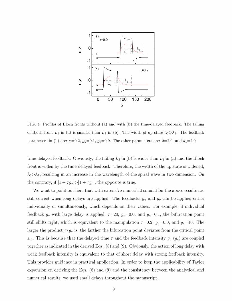
FIG. 4. Profiles of Bloch fronts without (a) and with (b) the time-delayed feedback. The tailing

of Bloch front L1 in (a) is smaller than L2 in (b). The width of up state λ2>λ1. The feedback

parameters in (b) are: τ=0.2, gu=0.1, gv=0.9. The other parameters are: δ=2.0, and a1=2.0.

time-delayed feedback. Obviously, the tailing L2 in (b) is wider than L1 in (a) and the Bloch

front is widen by the time-delayed feedback. Therefore, the width of the up state is widened,

λ2>λ1, resulting in an increase in the wavelength of the spiral wave in two dimension. On

the contrary, if |1 + τgu|>|1 + τgv|, the opposite is true.

We want to point out here that with extensive numerical simulation the above results are

still correct when long delays are applied. The feedbacks gu and gv can be applied either

individually or simultaneously, which depends on their values. For example, if individual

feedback gv with large delay is applied, τ=20, gu=0.0, and gv=0.1, the bifurcation point

still shifts right, which is equivalent to the manipulation τ=0.2, gu=0.0, and gv=10. The

larger the product τ∗gv is, the farther the bifurcation point deviates from the critical point

εc0. This is because that the delayed time τ and the feedback intensity gu (gv) are coupled

together as indicated in the derived Eqs. (8) and (9). Obviously, the action of long delay with

weak feedback intensity is equivalent to that of short delay with strong feedback intensity.

This provides guidance in practical application. In order to keep the applicability of Taylor

expansion on deriving the Eqs. (8) and (9) and the consistency between the analytical and

numerical results, we used small delays throughout the manuscript.

9

B. Transverse instability of front in two dimensions

In one dimensional case we concentrate on the front bifurcation by analyzing the relation

between the velocity of front and the parameter ε. A planar front could become curve in two

dimensions. It is necessary to consider further the stability of a planar front to transverse

perturbation, i.e. the transverse instability of planar front. In this section, we firstly obtain

patterns deep into the Bloch and Ising regions, and near the NIB bifurcation point without

time delay. Then we study the effects of time delay on the transverse instability of front.

Our emphasis is on controlling the transverse instability of front by applying appropriate

time delay.

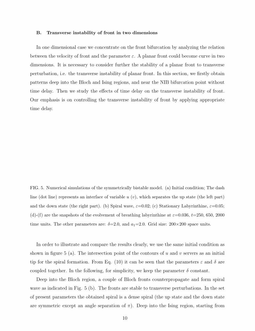
FIG. 5. Numerical simulations of the symmetrically bistable model. (a) Initial condition; The dash

line (dot line) represents an interface of variable u (v), which separates the up state (the left part)

and the down state (the right part). (b) Spiral wave, ε=0.02; (c) Stationary Labyrinthine, ε=0.05;

(d)-(f) are the snapshots of the evolvement of breathing labyrinthine at ε=0.036, t=250, 650, 2000

time units. The other parameters are: δ=2.0, and a1=2.0. Grid size: 200×200 space units.

In order to illustrate and compare the results clearly, we use the same initial condition as

shown in figure 5 (a). The intersection point of the contours of u and v servers as an initial

tip for the spiral formation. From Eq. (10) it can be seen that the parameters ε and δ are

coupled together. In the following, for simplicity, we keep the parameter δ constant.

Deep into the Bloch region, a couple of Bloch fronts counterpropagate and form spiral

wave as indicated in Fig. 5 (b). The fronts are stable to transverse perturbations. In the set

of present parameters the obtained spiral is a dense spiral (the up state and the down state

are symmetric except an angle separation of π). Deep into the Ising region, starting from

10

the initial condition [Fig. 5 (a)], the part near the domain center firstly evolves into a spiral

head. Then, the part behind the spiral head undergoes transverse instability and the fronts

interplay with each other, which resulting in a stationary labyrinthine pattern finally [Fig.

5 (c)]. In the stationary labyrinthine pattern the up states keep interconnection and own

identical widths. This process is similar with the observation in Refs. 15, 20. Near the NIB

bifurcation, the situation becomes more complex, where we observe a breathing labyrinthine

pattern. Fig. 5 (d)-(f) show three snapshots of the evolvement of breathing labyrinthine

at t=250, 650, 2000 time units. In this case, the up states can breakdown and reconnect.

Together with repulsive interaction between fronts, the widths of the up states increase and

decrease periodically, leading to the formation of a breathing labyrinthine pattern. The

most difference between the breathing labyrinthine and the stationary labyrinthine is that

in breathing labyrinthine case the up state does not interconnect entirely and its width

changes periodically. The present dynamics is similar with that of oscillatory spots.18

-1 0 1

-1

0

1

SL

BL

S

g v

gu

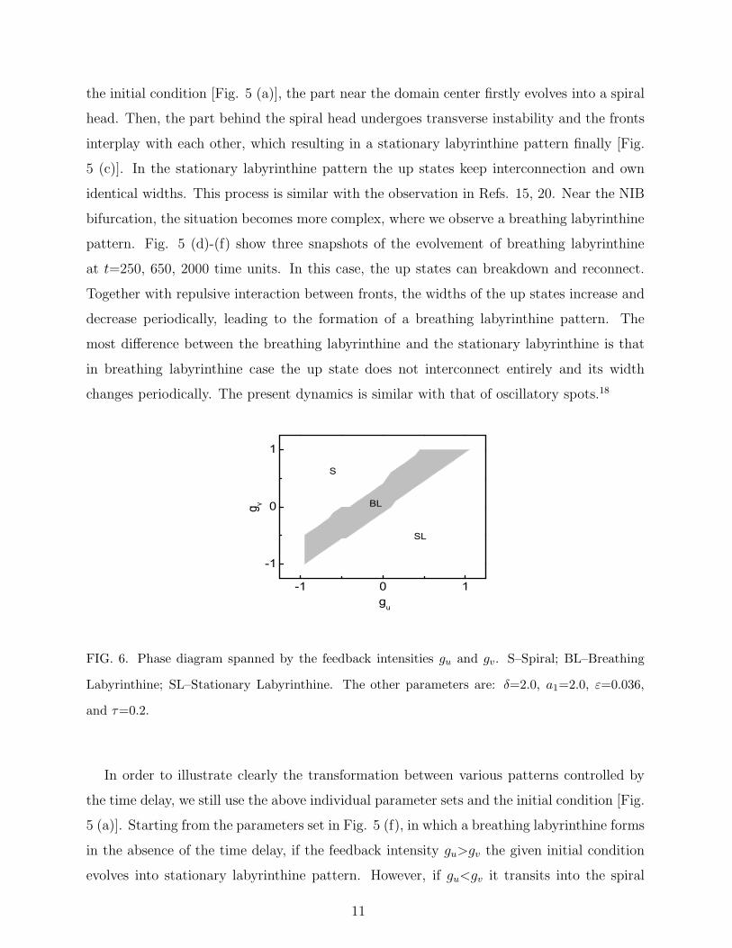
FIG. 6. Phase diagram spanned by the feedback intensities gu and gv. S–Spiral; BL–Breathing

Labyrinthine; SL–Stationary Labyrinthine. The other parameters are: δ=2.0, a1=2.0, ε=0.036,

and τ=0.2.

In order to illustrate clearly the transformation between various patterns controlled by

the time delay, we still use the above individual parameter sets and the initial condition [Fig.

5 (a)]. Starting from the parameters set in Fig. 5 (f), in which a breathing labyrinthine forms

in the absence of the time delay, if the feedback intensity gu>gv the given initial condition

evolves into stationary labyrinthine pattern. However, if gu<gv it transits into the spiral

11

pattern. So, the time delay can alter the critical value of transverse instability of planar

front (see the analysis below, Fig. 7). When applying the time delay to the system with

the parameters in Fig. 5 (b) and the same initial condition [Fig. 5 (a)], upon increasing

the ratio of gu/gv, it will develop into breathing labyrinthine and stationary labyrinthine

patterns successively. Similarly, if decreasing the ratio of gu/gv with the parameters as in

Fig. 5 (c), breathing labyrinthine and spiral patterns form in sequence. Figure 6 shows

a phase diagram spanned by the feedback intensities gu and gv, in which the gray region

represents the breathing labyrinthine pattern. It should be mentioned that the boundary

between spiral patterns and breathing labyrinthine patterns is not sharp because near this

boundary the arm of the spiral far away the tip could reflect upon touching the domain

boundary which leading to the breakdown of the arm. Here, we plot the boundary at which

perfect spirals could form. The wavelength of spiral can be adjusted by varying the feedback

parameters, as we have depicted above in the one dimensional case. The spiral period is

around 160 time units. So, the time delay is still applicable for controlling spiral patterns.

Therefore, by varying the ratio gu/gv one can realize the control of transverse instability of

planar front.

-0.1 0.0 0.1

-0.4

-0.2

0.0

0.2

0.4

c

32

10

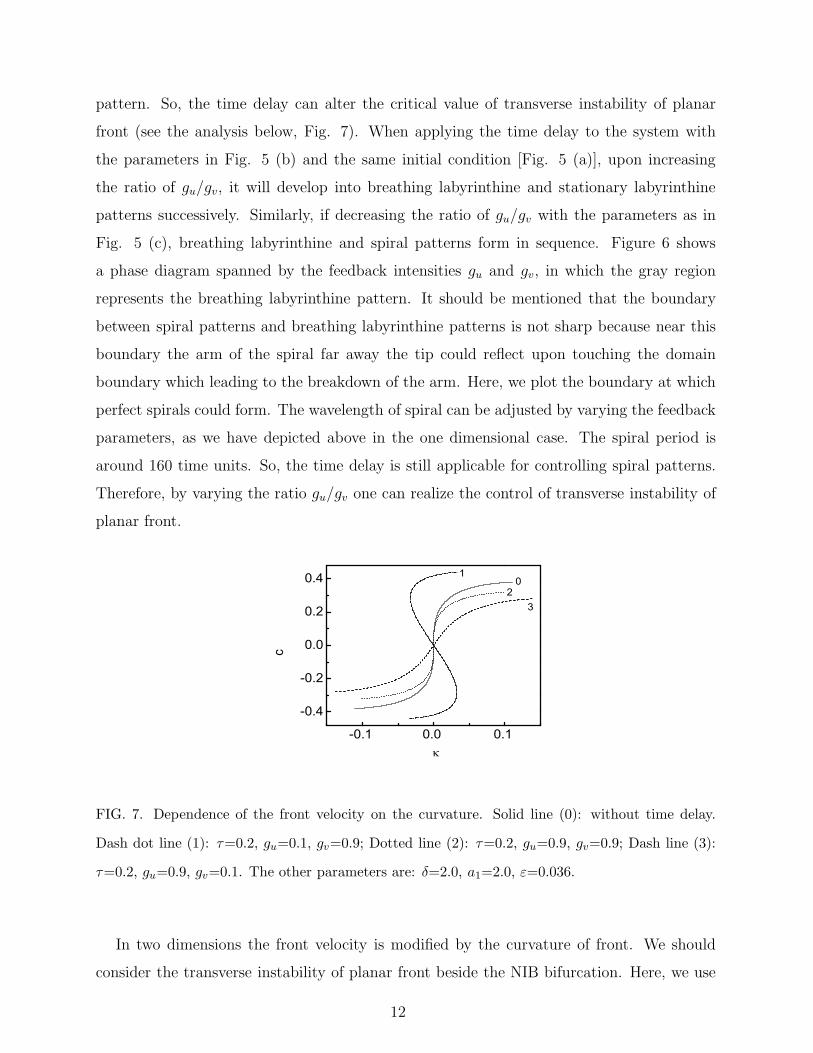
FIG. 7. Dependence of the front velocity on the curvature. Solid line (0): without time delay.

Dash dot line (1): τ=0.2, gu=0.1, gv=0.9; Dotted line (2): τ=0.2, gu=0.9, gv=0.9; Dash line (3):

τ=0.2, gu=0.9, gv=0.1. The other parameters are: δ=2.0, a1=2.0, ε=0.036.

In two dimensions the front velocity is modified by the curvature of front. We should

consider the transverse instability of planar front beside the NIB bifurcation. Here, we use

12

the algorithm in Ref. 20 to analyze the transverse instability of both Ising and Bloch fronts.

Under the modification by curvature, Eq. (10) can be written as:

cr(1 + τgu) + κ =3(cr(1 + τgv) + δκ)√

2q2[(cr(1 + τgv) + δκ)2 + 4εδq2]1

2

, (12)

here, cr is the normal velocity, and κ presents the curvature. Figure 7 shows a velocity-

curvature relation without and with the time delay. The solid line (0) represents the breath-

ing labyrinthine pattern at NIB bifurcation without time delay [Fig. 5 (f)]. At the center

of the plot, the slope of the curve indicates critical stability. If applying time delay with

identical intensities, such that gu=gv, the velocity changes, but the slope of the curve at the

center still keeps constant [dotted line (2)]. The stability of front to perturbation hardly

varies. So, one can still observe breathing labyrinthine pattern. When the feedback in-

tensities gu>gv, the above slope is positive [dash line (3)]. A front becomes unstable to

perturbation, and it finally evolves into stationary labyrinthine pattern. On the contrary, if

gu<gv, the mentioned slope becomes negative [dash dot line (1)], and a front keeps stable

upon suffering perturbation. We can obtain spiral pattern as shown above.

We now analyze further the stabilities of both Bloch and Ising fronts to perturbation when

applying the time delay. If the curvature is small, the normal velocity cr can be replaced by

cr=c0−dκ, in which c0 indicates the velocity of planar front. Here, the reduced parameter

d is not anymore a simple diffusion coefficient of activator as in excitable system.20 Its sign

determines the stability of a front to transverse perturbations. Inserting cr into Eq. (12)

and taking Taylor expansion, we can obtain the implicit expression about d:

1− d(1 + τgu) =3(

δ − d(1 + τgv))√2q2[c20(1 + τgv)2 + 4εδq2]1/2

− 3c20(1 + τgv)2(

δ − d(1 + τgv))√2q2[c20(1 + τgv)2 + 4εδq2]3/2

. (13)

It shows that the reduced parameter d is related with the control parameters δ, ε, a1, and

the feedback parameters in the model. If d is negative, the front becomes unstable upon

suffering transverse perturbations resulting in the labyrinthine pattern as shown in Fig. 5

(c). If d is positive, the front keeps stable to transverse perturbations leading to the spiral

wave as shown in Fig. 5 (b).

For the Ising front c0=0, so, we have:

1− d(1 + τgu) =3(

δ − d(1 + τgv))

2√2εδq3

. (14)

13

0.1

1

10

0.01 0.10.1

1

10

BD

B

FD

F

I

(a)

BD

B

FD

F

I

(b)

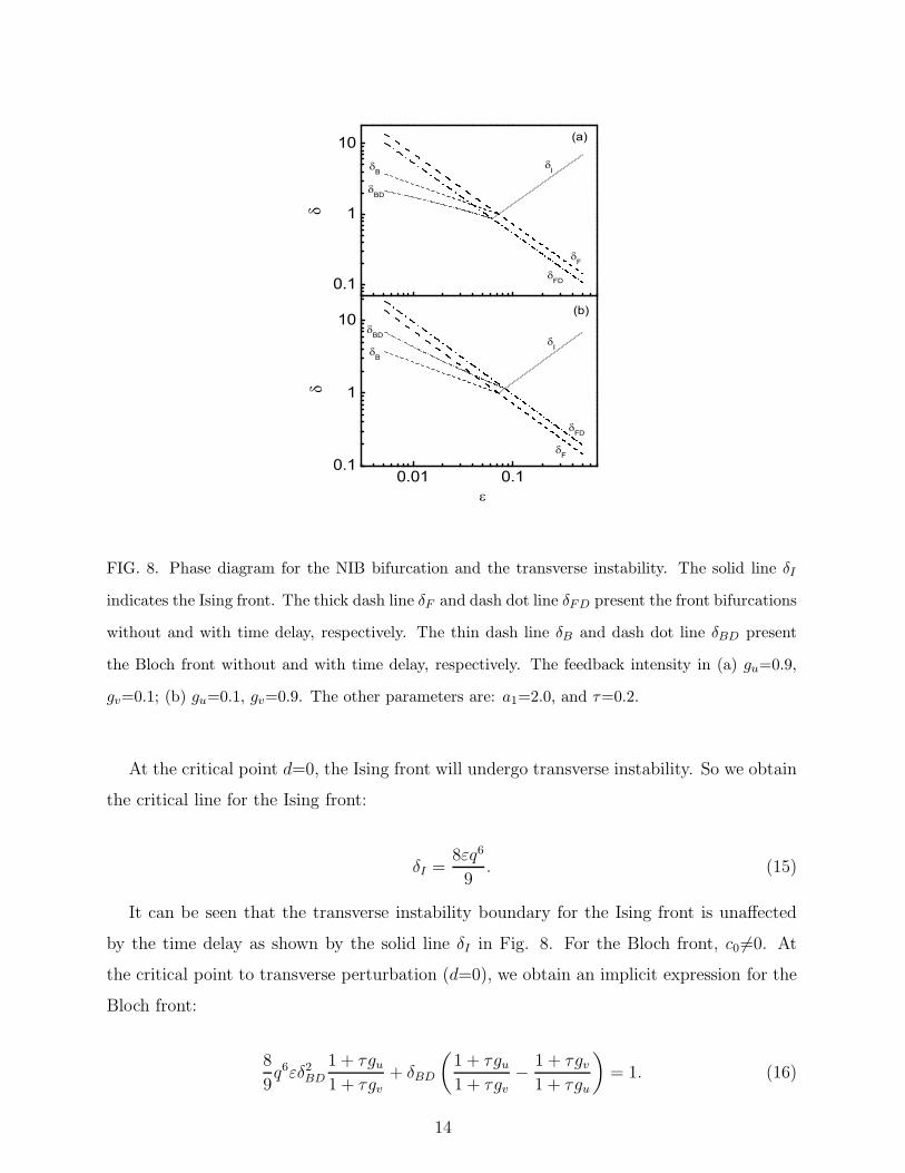
FIG. 8. Phase diagram for the NIB bifurcation and the transverse instability. The solid line δI

indicates the Ising front. The thick dash line δF and dash dot line δFD present the front bifurcations

without and with time delay, respectively. The thin dash line δB and dash dot line δBD present

the Bloch front without and with time delay, respectively. The feedback intensity in (a) gu=0.9,

gv=0.1; (b) gu=0.1, gv=0.9. The other parameters are: a1=2.0, and τ=0.2.

At the critical point d=0, the Ising front will undergo transverse instability. So we obtain

the critical line for the Ising front:

δI =8εq6

9. (15)

It can be seen that the transverse instability boundary for the Ising front is unaffected

by the time delay as shown by the solid line δI in Fig. 8. For the Bloch front, c0 6=0. At

the critical point to transverse perturbation (d=0), we obtain an implicit expression for the

Bloch front:

8

9q6εδ2BD

1 + τgu1 + τgv

+ δBD

(

1 + τgu1 + τgv

− 1 + τgv1 + τgu

)

= 1. (16)

14

The positive solution of δBD defines a boundary of the transverse instability of Bloch

front as shown by the thin dash dot lines in Fig. 8. From Eq. (16) it is found that the

competition between gu and gv alters the boundary. If gu>gv (gu<gv), the boundary moves

down (up) as shown in Fig. 8 (a) [Fig. 8 (b)]. When gu=gv the boundary stays constant as

the case without the time delay, which means that the time delay do not affect the critical

stability of Bloch front to transverse perturbations if the feedback intensity gu equals to gv.

IV. CONCLUSION AND REMARKS

In this work, we have studied the effects of the time-delayed feedback on the NIB bifurca-

tion in a bistable medium. The results have shown that the time-delayed feedback applied

to the activator and/or the inhibitor changes the critical point of NIB bifurcation. The

time delay alters the temporal scales of the reactions, therefore the velocity of Bloch front.

Large delay with weak feedback intensity is equivalent to small delay with strong feedback

intensity. The effect of time-delayed feedback on the activator opposes that on the inhibitor.

So there exists competition between the two feedbacks on controlling the NIB bifurcation.

Upon increasing the ratio gu/gv, the critical point of NIB bifurcation shifts left which could

result in a transition from Bloch front to Ising front, and vice versa. When time-delayed

feedback is applied individually to one of the species, positive and negative feedback make

the bifurcation point shift to different directions. In the two-dimensional case, the time de-

lay can change the stability of front to transverse perturbations. If gu<gv, it could stabilize

the front upon suffering transverse perturbation, and vice versa. In some sense applying the

time-delayed feedback to species is equivalent to changing their diffusion coefficients. Thus,

the wavelength of patterns can be controlled by properly using feedback parameters.

Although this FitzHugh-Nagumo model is a generic model, it has described successfully

the dynamics of pattern formation in bistable Ferrocyanide-Iodate-Sulfite reactions, such as

the bistable spirals, oscillating spots, and labyrinthine patterns15–18. These phenomena have

been attributed to the NIB front bifurcation. In this paper, we focus on the generalized

controlling scheme to the NIB bifurcation by applying time-delayed feedback to one or two

of the variables. The results have shown the flexibility of this strategy on controlling the

NIB bifurcation, therefore the transformation of patterns.

Many real chemical experiments, such as the ferroin-, Ru(bpy)3-, and cerium-catalyzed

15

Belousov-Zhabotinsky systems, are sensitive to visible and/or ultraviolet light.15,18,22,24,34–39

People have realized controlling of pattern formation by the time-delayed feedback in light-

sensitive chemical reactions. For example, by projecting the delayed image uniformly from

the feedback loop to the gel in the Petri dish, Kheowan and Zykov realized the controlling

of spiral waves in a thin layer of the light-sensitive Belousov-Zhabotinsky reaction.37,38 The

radius of the attractor for meandering spiral waves can be effectively manipulated by varying

the delayed time in the feedback loop. Karl Vanag et al observed oscillatory cluster pat-

terns in a light-sensitive Ru(bpy)3-catalyzed Belousov-Zhabotinsky reaction.39 The catalyst

Ru(bpy)3 is light-sensitive. Thus, a proper illumination of the active chemical substrate

can be used for spatial control of the inhibiting process (Br−). Our results have also con-

firmed that applying the time-delayed feedback only to the inhibitor is enough to control

the pattern formation. In a light-sensitive ferrocyanide-iodate-sulphite reaction, Lee et al

observed the pattern transformation via NIB bifurcation by changing the flow rate or the

input ferrocyanide concentration.15,18 Our results have shown that applying the time-delayed

feedback for controlling the NIB bifurcation, from the experimental viewpoint, is equivalent

to changing the residence time or the input ferrocyanide concentration. We hope that our

results can be verified in one of the light-sensitive reactions with patterned (not uniform)

illumination after feedback loop. The feedback loop should mainly include: 1) CCD camera,

2) video recorder, 3) computer which implements the algorithm of eqs. (3) and (4) and out-

puts the results (patterned images with appropriate intensity) to a projector, 4) projector

which projects the patterned images inputted from the computer to the chemical substrate.

ACKNOWLEDGMENTS

This work is supported in part by Hong Kong Baptist University and the Hong Kong

Research Grants Council. Y. F. He also acknowledges the National Natural Science Founda-

tion of China with Grant No. 10975043, 10947166, 10775037, and the Research Foundation

of Education Bureau of Hebei Province, China (Grant No. 2009108).

∗ Email:[email protected]

1 C. C. Cross and P. C. Hohenberg, Rev. Mod. Phys. 65, 851 (1993).

16

2 A. J. Koch and H. Meinhardt, Rev. Mod. Phys. 66, 1481 (1994).

3 J. Horvath, I. Szalai, and P. De Kepper, Science 324, 772 (2009).

4 Y. F. He, B. Q. Ai, and B. B. Hu, J. Chem. Phys. 132, 184516(2010).

5 I. R. Epstein, J. A. Pojman, and O. Steinbock, Chaos 16, 037101 (2006).

6 A. Kothe. V. S. Zykov, and H. Engel, Phys. Rev. Lett. 103, 154102 (2009).

7 V. S. Zykov, physica D 238, 931 (2009).

8 A. Hagberg and E. Meron, Phys. Rev. Lett. 78, 1166 (1997).

9 A. Hagberg and E. Meron, Chaos, 4, 477 (1994).

10 B. Marts, K. Martinez, and A. L. Lin, Phys. Rev. E 70, 056223 (2004).

11 R. E. Goldstein, D. J. Muraki, and D. M. Petrich, Phys. Rev. E 53, 3933 (1996).

12 M. Bar, A. Hagberg, E. Meron, and U. Thiele, Phys. Rev. E 62, 366 (2000).

13 G. Haas, M. Bar, I. G. Kevrekidis, P. B. Rasmussen, H. H. Rotermund, and G. Ertl, Phys. Rev.

Lett. 75, 3560 (1995).

14 M. Bar, S. Nettesheim, H. H. Rotermund, M. Eiswirth, and G. Ertl, Phys. Rev. Lett. 74, 1246

(1995).

15 K. J. Lee, W. D. McCormick, Q. Ouyang, and H. L. Swinney, Science 261, 192 (1993).

16 G. Li, Q. Ouyang, and H. L. Swinney, J. Chem. Phys. 105, 10830 (1996).

17 I. Szalai and P. De Kepper, J. Phys. Chem. A 112, 783 (2008).

18 K. J. Lee, W. D. McCormick, J. E. Pearson, and H. L. Swinney, Nature 369, 215 (1994).

19 A. Hagberg and E. Meron, Physica D 123, 460 (1998).

20 A. Hagberg and E. Meron, Phys. Rev. Lett. 72, 2494 (1994).

21 E. Ott, C. Grebogi, and J. A. Yorke, Phys. Rev. Lett. 64, 1196 (1990).

22 O. U. Kheowan, V. S. Zykov, and S. C. Muller, Phys. Chem. Chem. Phys. 4, 1334 (2002).

23 V. S. Zykov, A. S. Mikhailov, and S. C. Muller, Phys. Rev. Lett. 78, 3398 (1997).

24 W. Q. Guo, C. Qiao, Z. M. Zhang, Q. Ouyang, and H. L. Wang, Phys. Rev. E 81, 056214

(2010).

25 L. G. Stanton and A. A. Golovin, Phys. Rev. E 76, 036210 (2007).

26 Yu. A. Logvin and N. A. Loiko, Phys. Rev. E 56, 3803 (1997).

27 S. Sen, P. Ghosh, S. S. Riaz, and D. S. Ray, Phys. Rev. E 80, 046212 (2009).

28 Q. S. Li and H. X. Hu, J. Chem. Phys. 127, 154510 (2007).

29 F. M. Schneider, E. Scholl, and M. A. Dahlem, Chaos 19, 015110 (2009).

17

30 M. Gassel, E. Glatt, and F. Kaiser, Phys. Rev. E 77, 066220 (2008).

31 A. G. Balanov, V. Beato, N. B. Janson, H. Engel, and E. Scholl, Phys, Rev. E 74, 016214

(2006).

32 Q. S. Li and Lin Ji, Phys. Rev. E 69, 046205 (2004).

33 M. Kim, M. Bertram, M. Pollmann, A. von Oertzen, A. S. Mikhailov, H. H. Rotermund, and

G. Ertl, Science 292, 1357 (2001).

34 R. Tth, V. Gaspar, A. Belmonte, M. C. O’Connell, A. Taylor, and D. K. Scott, Phys. Chem.

Chem. Phys. 2, 413 (2000).

35 V. K. Vanag, Y. Mori, and I. Hanazaki, J. Phys. Chem. 98, 8392 (1994).

36 M. Hildebrand, H. Skødt, and K. Showalter, Phys. Rev. Lett. 87, 088303 (2001).

37 O. U. Kheowan, V. Gaspar, V. S. Zykov, and S. C. Muller, Phys. Chem. Chem. Phys. 3, 4747

(2001).

38 V. S. Zykov, G. Bordiougov, H. Brandtstadter, I. Gerdes, and H. Engel, Phys. Rev. Lett. 92,

018304 (2004).

39 V. K. Vanag, L. F. Yang, M. Dolnik, A. M. Zhabotinsky, and I. R. Epstein, Nature 406, 389

(2000).

18