Pathogen Persistence in the Environment and Insect-Baculovirus Interactions: Disease-Density Thresholds, Epidemic Burnout, and Insect Outbreaks

Pathogen Persistence in the Environment and Insect-Baculovirus Interactions: Disease-DensityThresholds, Epidemic Burnout, and Insect Outbreaks.Author(s): Emma Fuller, Bret D. Elderd, Greg DwyerReviewed work(s):Source: The American Naturalist, Vol. 179, No. 3 (March 2012), pp. E70-E96Published by: The University of Chicago Press for The American Society of NaturalistsStable URL: http://www.jstor.org/stable/10.1086/664488 .Accessed: 10/02/2012 09:32

Your use of the JSTOR archive indicates your acceptance of the Terms & Conditions of Use, available at .http://www.jstor.org/page/info/about/policies/terms.jsp

JSTOR is a not-for-profit service that helps scholars, researchers, and students discover, use, and build upon a wide range ofcontent in a trusted digital archive. We use information technology and tools to increase productivity and facilitate new formsof scholarship. For more information about JSTOR, please contact [email protected].

The University of Chicago Press and The American Society of Naturalists are collaborating with JSTOR todigitize, preserve and extend access to The American Naturalist.

http://www.jstor.org

vol. 179, no. 3 the american naturalist march 2012

E-Article

Pathogen Persistence in the Environment and Insect-Baculovirus Interactions: Disease-Density Thresholds,

Epidemic Burnout, and Insect Outbreaks

Emma Fuller,1,* Bret D. Elderd,2 and Greg Dwyer1,†

1. Department of Ecology and Evolution, University of Chicago, Chicago, Illinois 60637; 2. Department of Biological Sciences,Louisiana State University, Baton Rouge, Louisiana 70803

Submitted July 26, 2011; Accepted October 31, 2011; Electronically published January 26, 2012

Dryad data: http://dx.doi.org/10.5061/dryad.7r1v08r8.

abstract: Classical epidemic theory focuses on directly transmittedpathogens, but many pathogens are instead transmitted when hostsencounter infectious particles. Theory has shown that for such dis-eases pathogen persistence time in the environment can stronglyaffect disease dynamics, but estimates of persistence time, and con-sequently tests of the theory, are extremely rare. We consider theconsequences of persistence time for the dynamics of the gypsy mothbaculovirus, a pathogen transmitted when larvae consume foliagecontaminated with particles released from infectious cadavers. Usingfield-transmission experiments, we are able to estimate persistencetime under natural conditions, and inserting our estimates into astandard epidemic model suggests that epidemics are often termi-nated by a combination of pupation and burnout rather than byburnout alone, as predicted by theory. Extending our models to allowfor multiple generations, and including environmental transmissionover the winter, suggests that the virus may survive over the longterm even in the absence of complex persistence mechanisms, suchas environmental reservoirs or covert infections. Our work suggeststhat estimates of persistence times can lead to a deeper understandingof environmentally transmitted pathogens and illustrates the use-fulness of experiments that are closely tied to mathematical models.

Keywords: host-pathogen, Lymantria dispar, nucleopolyhedrovirus,threshold theorem, insect outbreaks, environmental transmission,complex dynamics.

Introduction

In classical epidemic models, transmission results fromcontact between healthy and infectious hosts (Kermackand McKendrick 1927), but for many animal pathogens,transmission instead occurs when hosts contact infectious

* Present address: The Nature Conservancy, 1917 First Avenue, Seattle, Wash-

ington 98101.†

Corresponding author; e-mail: [email protected].

Am. Nat. 2012. Vol. 179, pp. E70–E96. � 2012 by The University of Chicago.

0003-0147/2012/17903-53215$15.00. All rights reserved.

DOI: 10.1086/664488

particles in the environment (Ebert et al. 1996; Hall et al.2005; Mathiason et al. 2009). For such diseases, theory hasshown that pathogen persistence time in the environmentis an important determinant of whether an epidemic willoccur (Breban et al. 2009), but applications of the theoryrequire estimates of persistence times. Estimating persis-tence times from observations of disease spread in natureis difficult, because losses due to pathogen breakdown maybe outweighed by gains due to pathogen particles pro-duced from new infections (Woods and Elkinton 1987),making it hard to distinguish persistence from infectious-ness. Meanwhile, field experiments that can disentanglepersistence and infectiousness are often impossible (Dob-son and Meagher 1996). Persistence-time estimates aretherefore rare, and so applications of the theory are cor-respondingly rare.

For baculovirus diseases of insects in contrast, field ex-periments are entirely feasible (D’Amico and Elkinton1995; Goulson et al. 1995; Hails et al. 2002; Georgievskaet al. 2010). In many insects, baculoviruses are transmittedwhen larvae consume foliage contaminated with the in-fectious cadavers of other larvae, and infection generallyleads to death (Cory and Myers 2003). This simple biologymakes it possible to experimentally quantify transmissionin the field (Dwyer 1991; Zhou et al. 2005; Elderd et al.2008), and extending this type of experiment to also mea-sure baculovirus persistence time is straightforward. Wetherefore used a field-transmission experiment to estimatethe persistence time of a baculovirus of the gypsy moth,Lymantria dispar, and we used our estimate in mathe-matical models to show how persistence time affects bac-ulovirus epidemics and gypsy moth outbreaks.

Experiments that show evidence of baculovirus decayhave a 45-year history (Jaques 1967), yet to our knowledgebaculovirus persistence time under natural conditions inthe field has never been estimated. Previous experiments

Pathogen Persistence in the Environment E71

generally did not consider estimation, instead simply test-ing whether a treatment alters the effect of exposure timeon the infection rate (Jaques 1967, 1968, 1972; Broome etal. 1974; Elnagar and Abul-Nasr 1980; Biever and Hostetter1985; Roland and Kaupp 1995; Webb et al. 1999, 2001;Raymond et al. 2005). Apparently as a result, most ex-periments were not designed in a way that permits separateestimation of persistence time and infectiousness, as weexplain in the appendix. Also, previous experiments havegenerally followed biological control programs in usingpurified virus (Hunter-Fujita et al. 1998), which may leadto artificially reduced persistence times. In our experi-ments, we mimicked natural transmission by using infec-tious cadavers, and comparing our estimate of persistencetime to estimates based on data for purified virus (Webbet al. 1999, 2001) shows that purified gypsy moth virusbreaks down roughly twice as fast as infectious cadavers.

Our estimate of virus persistence time is important be-cause it helps us to understand both virus epidemics andinsect outbreaks. To show this, we first inserted our es-timate into an epidemic model, modified to allow pupationto terminate transmission, and we compared the predic-tions of this model to two predictions of epidemic theory(Keeling and Rohani 2007). The first prediction is thatthere will be a minimum host population at which anepidemic will occur, the disease density (or host density)threshold. The second prediction is that epidemics willend because of a lack of infected hosts rather than becauseof a lack of susceptible hosts, so-called epidemic burnout.If persistence time is sufficiently high, however, the diseasethreshold may be so low that whether an epidemic occurswill be determined by the initial density of the pathogeninstead of by the threshold. Alternatively, if persistencetime is sufficiently low, epidemics will end because of hostpupation rather than burnout. Our models show that thepersistence time of the gypsy moth virus is short enoughthat the disease-density threshold is a useful statistic, butit is also short enough that pupation is often as importantas burnout in ending epidemics.

These effects can modulate outbreaks because gypsymoth population dynamics are partly driven by virus ep-idemics (Dwyer et al. 2004; Bjornstad et al. 2010). Ex-tending our single-epidemic model to allow for multiplehost generations shows that shorter persistence times pro-duce less severe outbreaks. Moreover, our estimate of per-sistence time leads to long-term virus survival in the mod-els, even though the models include only simplemechanisms of overwinter survival, notably external con-tamination of egg masses. This is important because effortsto explain long-term baculovirus persistence often em-phasize more complex survival mechanisms, such as soilreservoirs (Thompson et al. 1981; Hochberg 1989; Fuxaand Richter 2007) and covert infections (Myers et al. 2000;

Burden et al. 2003). Our model instead suggests that res-ervoirs and covert infections may not be necessary to ex-plain baculovirus persistence, either in the gypsy moth orin other insects (Moreau and Lucarotti 2007).

Material and Methods

Baculovirus Ecology and Epidemic Models

Like many outbreaking insects (Hunter 1991), gypsymoths have only one generation per year, with five instars(larval stages) in males and six in females. In southwesternMichigan, where we carried out our experiments, larvaehatch in late April or early May. Pupation occurs in mid-July, and the insect overwinters in the egg (Elkinton andLiebhold 1990).

In the spring, some hatchlings (or neonates) becomeinfected, later releasing infectious occlusion bodies thatbegin the epidemic (Woods and Elkinton 1987). Unin-fected larvae that consume a large enough dose of thevirus die 7–21 days after infection and release occlusionbodies onto the foliage for consumption by other larvae(Cory and Myers 2003). The most important round oftransmission thus occurs when virus produced by infectedneonates infects larvae in the third and fourth instars(Woods and Elkinton 1987). In our experiments, we there-fore measured transmission from infected neonates to un-infected fourth instars.

Although models of directly transmitted diseases assumethat transmission occurs only through contact betweeninfected and uninfected hosts, we can nevertheless use suchmodels for baculoviruses by using the infectious-host classin the models to represent infectious cadavers. The modelthat we use is therefore a modification of the well-knownsusceptible-exposed-infected-removed model (Keeling andRohani 2007), extended to allow for host heterogeneity ininfection risk, an important factor in the transmission ofthe gypsy moth virus (Dwyer et al. 1997). This model isa variant of models previously used by the second andthird authors, extended to allow for variance in the dis-tribution of the time between infection and death, a var-iance that we previously assumed was very low (Dwyerand Elkinton 1993; Elderd et al. 2008). Because it allowsfor nonzero variance in this distribution, the model thatwe use here is slightly more realistic, and it has the ad-vantage of being more stable when numerically integratedon a computer:

E72 The American Naturalist

2C

dS S(t)¯p � nSP , (1)( )dt S(0)

2C

dE S(t)1 ¯p nSP � mdE , (2)1( )dt S(0)

dEi p mdE � mdE (i p 2, … , m), (3)i�1 idt

dPp mdE � mP. (4)mdt

Here S is the density of uninfected or susceptible hosts,and P is the density of infectious cadavers. Gypsy mothlarvae vary in the dose of virus needed to cause infection(Dwyer et al. 1997), as well as in feeding behavior (Parkeret al. 2010), leading to variability in overall infection risk(Dwyer et al. 2005; Elderd et al. 2008). We therefore as-sume that transmission rates follow a probability distri-bution with mean and coefficient of variation C. Ton

describe the probability distribution that models the timebetween infection and death, we follow standard practicein dividing the exposed class into m classes, such thatEi

the average speed of kill is and the rate at which in-1/ddividuals move from one class to the next is (Keelingmd

and Rohani 2007). The total time in the exposed classesis then equal to the sum of m exponential distributions,each with mean . This sum follows a gamma dis-1/(md)tribution with mean and variance , so that the21/d 1/(md )variance declines as m increases. We can therefore controlthe variance on the distribution of speeds of kill by varyingm. We assume days, with , based on1/d p 12 m p 20observations of speeds of kill of infected larvae (G. Dwyer,unpublished data). This model requires integer values ofm, but in our case changing m by 1 instead of, say, by 0.5,has only a tiny effect on the epidemic. Also, because hatch-ling larvae are much smaller than later instars, we allowfor a simple form of stage structure by assuming thatinfected hatchlings produce smaller cadavers than laterinstars.

Once larvae reach the final exposed class m, they dieand become infectious cadavers P. Cadavers break downat rate m, so estimating m was the goal of our experiments.The average persistence time of the virus is , so that1/mlarge values of m produce short persistence times. Decaylikely occurs because the virus is destroyed or inactivatedby the ultraviolet rays in sunlight (Ignoffo et al. 1977),but the virus may also be washed off foliage by rain(D’Amico and Elkinton 1995). Versions of this model havesurvived extensive testing with both experimental and ob-servational data for the gypsy moth virus (Dwyer and Elk-inton 1993; Dwyer et al. 1997, 2005; Elderd et al. 2008).

We therefore use it to understand the implications of ourparameter estimates.

Field Experiments

Field observations of baculovirus populations cannot eas-ily be used to estimate decay rates, because losses of virusdue to decay are often offset by inputs of virus due tonew virus-caused deaths (Woods and Elkinton 1987). Pre-vious field studies have therefore simply observed thatvirus is present at two points in time, usually one im-mediately following an epidemic and one a year or morelater, with the conclusion that virus particles can some-times survive for a year or more (Tanada and Omi 1974;Entwistle and Adams 1977; Young et al. 1977; Podgwaiteet al. 1979; Olofsson 1988).

An experimental approach might therefore be more ef-fective, but most experiments that vary exposure time haveused only a single virus density (Broome et al. 1974; El-nagar and Abul-Nasr 1980; Biever and Hostetter 1985;Raymond et al. 2005). As we show in the appendix, thesesingle-density experiments generally preclude estimationof decay rates using standard models. In standard models,infection rates are a nonlinear function of both exposuretime and virus density, and the effects of the two cannotbe distinguished unless they are varied independently (Sunet al. (2004) avoid this problem by instead back-calculatingvirus densities using dose-response data collected in anadditional experiment, but their approach may underes-timate parameter uncertainty; appendix). The few exper-iments that varied virus density and exposure time in-dependently did not attempt to estimate the decay rate(Jaques 1967, 1972; Webb et al. 1999, 2001), possibly be-cause of the difficulties of using the nonlinear fitting rou-tines that are required for estimating parameters from frac-tional data. Also, experiments with baculoviruses havehistorically used purified virus, because the point of manyexperiments is to test insecticidal sprays, which usuallyincorporate only purified virus and because some authorshave perhaps assumed that infectious cadavers would pro-duce data that are so noisy as to be uninterpretable. Animportant feature of natural transmission, however, is thatinfectious cadavers include insect body parts that mayblock UV (Capinera et al. 1976), and so experiments usingpurified virus may produce artificially inflated estimatesof the decay rate. The use of infectious cadavers is thereforeincreasingly common, but for all the infectious-cadaverexperiments of which we are aware, it is unclear whetherthe initially infected larvae were all dead when decay began,so virus inputs and virus losses probably occurred at thesame time (Goulson et al. 1995; Hails et al. 2002; Zhouet al. 2005; Georgievska et al. 2010; the one exception,Roland and Kaupp 1995, only compared decay inside a

Pathogen Persistence in the Environment E73

forest to decay on the edge of the forest and so includedneither exposure-time treatments nor density treatments;it therefore also cannot be used to estimate decay time).Data from such experiments have the same problem asdata from observations of epidemics, namely that decayis confounded with transmission, and apparently as a resultin some cases it was impossible to detect the effects ofexposure time (Goulson et al. 1995; Hails et al. 2002).

Our experiments were designed to circumvent these dif-ficulties. First, to avoid an inflated estimate of naturaldecay, we used infectious cadavers. We then used six toeight replicates of each treatment, depending on the ex-periment, which was enough that the uncertainty in ourdata was reasonably low, in turn permitting detection ofvirus decay. Meanwhile, two previous purified-virus ex-periments produced usable decay data for the gypsy mothbaculovirus (Webb et al. 1999, 2001), and reanalysis ofthose data confirmed that purified virus does indeed havea significantly shorter persistence time than infectious ca-davers. Using infectious cadavers also allowed us to moreaccurately estimate the transmission rate , which wen

needed to estimate the density threshold. Because is es-n

sentially infection risk, it is affected by feeding behavior(Dwyer et al. 2005), including the ability of gypsy mothlarvae to detect and avoid infectious cadavers (Capineraet al. 1976; Parker et al. 2010). Unbiased estimation of n

therefore required that we allow larvae to feed on virus-contaminated foliage under natural conditions, and soagain it was important to use infectious cadavers.

Second, to avoid the obscuring effects of additions ofvirus while decay is occurring, we only allowed decay tobegin after all of the initially infected larvae were dead. Todo this, we placed the infected larvae on the foliage, andwe enclosed larvae and foliage in mesh bags. The bagswere necessary to prevent larvae from dispersing to otherbranches, but as we will show, they also effectively pre-vented decay. Once we were sure that the infected larvaewere dead, we allowed for decay by removing the bags.After the virus had decayed for the requisite time, we addedhealthy larvae to the foliage, using new bags, which pre-vented further decay during transmission. To prevent lateradditions of virus due to the deaths of secondarily infectedlarvae, we allowed the uninfected larvae to feed for only1 week, a period short enough that no secondarily infectedlarvae died during the experiment. At the end of the week,we removed the initially uninfected larvae to the lab, ter-minating transmission, and we recorded the number oflarvae dying of the virus. Our experiments therefore al-lowed for only one round of transmission (note that incontrast, our epidemic model, eqq. [1]–[4], allows formultiple rounds of infection, but this difference does notrestrict our analyses in any way). We then used the fractioninfected to estimate the transmission parameters and Cn

and the viral decay rate m by fitting the model equations(1)–(4) to the data.

To ensure that the initially uninfected larvae were indeeduninfected, we reared them in the lab on artificial dietusing surface-disinfected eggs. Surface disinfection for 90minutes in 10% formalin is effective in preventing infec-tion (Doane 1969; Elderd et al. 2008). Because small dif-ferences in developmental stage within an instar can altersusceptibility (Grove and Hoover 2007), we synchronizedlarvae by collecting them shortly before eclosion to thefourth instar, holding them for 24–48 hours at 4�C untilwe had enough larvae to carry out an experiment and thenallowing all larvae to molt to the fourth instar at roomtemperature. The effect was that all of our uninfected lar-vae molted to the fourth instar within roughly 24 hoursof each other.

To produce infected larvae, we placed neonates in cupswith diet contaminated with a high virus dose (Dwyer etal. 2005). By using a plaque-purified virus clone, we en-sured that variability in the virus would play little role(Elderd et al. 2008). We then held these infected larvae at28�C for 5 days before placing them on foliage in the field.Because infected neonates do not molt to the second instar(Park et al. 1996), it was possible to identify and discardthe small number of larvae that did not become infected.Because our emphasis was on estimating the decay raterather than heterogeneity in infection risk, we reducedheterogeneity by using larvae from a U.S. Department ofAgriculture colony that has been reared in the laboratoryfor decades (Dwyer et al. 1997).

The infected larvae were placed on leaves of naturallyoccurring red oaks (Quercus rubra), a “most-favored’’ hostplant of the gypsy moth (Barbosa and Krischik 1987).Experimental trees were located in the Lux Arbor Reserveof the Kellogg Biological Station, in Delton, Michigan(42�28′N, 85�28′W). This site had negligible levels of gypsymoths or virus during the years of our study (Elderd etal. 2008). Each larva-laden branch was enclosed withinbags made of spun-bonded polyester or Reemay, whichhas only modest effects on humidity and temperature (Lip-man et al. 1992). We used virus densities of 25 and 50cadavers per branch, a range that is sufficient to producemeasurable infection rates (Dwyer et al. 2005), and thatfalls within the range of densities observed in nature(Woods and Elkinton 1987). We also included a controltreatment containing no infected larvae, to test whetherinfections could be due to naturally occurring virus. In-fection rates on the control branches were close to zero.

Five days after deployment the infected larvae were alldead, so we removed the bags from the branches, exposingthe virus-contaminated foliage to the environment. Be-cause, as we will show, decay inside the bags is negligible,no decay occurred until the bags were removed from the

E74 The American Naturalist

foliage, so all virus had already been added to the foliagewhen decay began. We used exposure times of 0, 1, 3, and7 days in 2007, each replicated six times. However, the2007 data suggested that our estimates would be moreaccurate if we used more replicates and eliminated thelongest exposure-time treatment, so in 2008 we used treat-ments of 0, 1 and 3 days, each replicated eight times. Afterexposing the cadavers, we enclosed the branches withinnew bags to prevent transmission through contact withthe mesh, and we released 20 uninfected fourthth instarsonto each branch. We allowed the uninfected larvae tofeed for 7 days, after which we placed them in individualdiet cups for 3 weeks to determine whether they wereinfected. Infected larvae are usually recognizable becausethey liquefy, but in cases of uncertainty we examined larvaeunder a light microscope, where the occlusion bodies wereclearly visible at #400 (Miller 1997).

In 2007, many initially uninfected larvae were lost topredation by other insects, notably stink bugs (Heterop-tera: Pentatomidae), and in any case the experimental de-sign was still rough. In 2008 we used a more powerfuldesign and stink bug predation was low, and so our es-timate of the decay rate from 2008 is thus more reliable.As we will show, however, virus decay was detectable inboth years, and so we include both data sets. Also, in 2007the experiment was carried out in July, while in 2008 theexperiment was carried out in June, but previous workhas made clear that the timing of this type of experimentwithin the summer has no effect on the results (Dwyer etal. 2005).

Statistical Tests

To estimate the decay rate m and the transmission param-eters and C, we simplified the single-epidemic model ton

match the conditions of our experiments. After the un-infected larvae were placed on the branches, no more viruswas added, and as we will show the virus does not decaywhile the foliage is in a bag, so we can set the rate ofchange of infectious cadavers inside the bags .dP/dt p 0We allowed virus transmission for 7 days ( ), and sot p 7we integrate equation (1) for the host population from 0to . Equation (1) can then be solved to give the fractiontof susceptible hosts S remaining after transmission hasended (appendix). Because our main interest was in de-tecting virus decay, our statistical analyses were designedto determine whether allowing for improved them 1 0model’s fit to the data. We therefore considered two ver-sions of the model, one with and one with .m 1 0 m p 0If we assume , we havem 1 0

ˆS(t) 22 �mT �1/Cˆ¯p (1 � nC P(0)e t) . (5)S(0)

If we assume , we havem p 0

ˆS(t) 22 �1/Cˆ¯p (1 � nC P(0)t) . (6)S(0)

Here and are the densities of uninfected hosts atˆS(0) S(t)the beginning and the end of the transmission period,respectively. The initial density of infectious cadavers isthen , and T is the length of time that virus-contam-P(0)inated leaves were exposed to the environment beforetransmission began. Following equation (4) for the infec-tious-cadaver population, we thus assume that, in the ab-sence of new virus deaths, the virus population decaysexponentially when exposed to the environment.

Monte Carlo simulations have shown that estimates ofheterogeneity C using this type of experiment have smallerconfidence intervals if the experiment includes a largernumber of virus densities (G. Dwyer, unpublished data).Because our emphasis was on estimating the decay rate m,however, we sacrificed a larger number of virus densitiesin favor of a larger number of exposure-time treatments.Similarly, values of C tend to be higher for feral larvaethan for laboratory larvae (Dwyer et al. 1997, 2005), butbecause of our emphasis on estimating the decay rate, weused laboratory larvae to reduce overall variability and soto increase statistical power. Consequently, as we will show,models that assume fit our data better than modelsC r 0that assume . If we allow , then the model forC 1 0 C r 0

ism 1 0

ˆS(t)�mTˆp exp (�nP(0)e t), (7)

S(0)

whereas for , the model ism p 0

ˆS(t) ˆp exp (�nP(0)t). (8)S(0)

In fact, 11 previous experiments by the second and thirdauthors and colleagues have demonstrated that, for thegypsy moth, heterogeneity , even for laboratory lar-C 1 0vae (Dwyer et al. 1997, 2005; Elderd et al. 2008). Accord-ingly, even though in the interests of statistical rigor weemphasize the fit of models for which , we alsoC p 0report results for the case for which . Fortunately,C 1 0our estimates of the decay rate m in the two cases are verysimilar.

In our statistical models we assume that no virus decayoccurs within the mesh bags. To test this, in 2007 weincluded a treatment in which all infected larvae were dead7 days before the experiment began, but for which theinfectious cadavers were never exposed to the environ-

Pathogen Persistence in the Environment E75

ment. We thus allowed for a week of virus decay, but onlywithin a bag (although we again put new bags on beforeadding uninfected larvae, as in the other treatments). Aswith the other treatments, this additional treatment wasreplicated six times. For the 2007 data, we therefore in-cluded a model with a separate rate for decay inside thebag (see appendix for the models).

To estimate m, , and C in equations (5)–(8), we fit eachn

equation to the data using maximum likelihood, using thenonlinear-fitting routines optim and optimize in the R pro-gramming language (R Development Core Team 2009).We used a binomial likelihood function, as is appropriatefor mortality data (McCullagh and Nelder 1989), but toallow for the possibility of overdispersion, we calculateda variance-inflation factor (Burnham and Anderson 2002).The variance-inflation factor is the goodness-of-fit x2 sta-tistic of the global model, in this case equation (5), dividedby the degrees of freedom (McCullagh and Nelder 1989).For the 2007 data the variance-inflation factor was 2.23,while for the 2008 data it was 1.89. These values are smallenough (!4) to suggest that there was no systematic lackof fit, but large enough that we used them to adjust ourAICc values, by dividing each AICc value by the varianceinflation factor (Burnham and Anderson 2002). This sta-tistic is known as the quasi-likelihood AIC, or QAICc, butfor brevity we refer to it as an AICc score. By choosingthe best model using the AICc, we tested whether the mod-els that assume provide a better explanation for them 1 0data than the models that assume . The lower them p 0AICc score, the better the model (Burnham and Anderson2002).

We calculated 95% confidence intervals on the decayrate m using bootstrapping (Efron and Tibshirani 1994),to determine whether the confidence intervals overlapped0. To do this we randomly selected replicates with replace-ment from within a given year’s data until we had as manyreplicates as used in that year, and then we recalculatedthe parameter values. This procedure was repeated 1,000times, and the resulting distribution provided 95% con-fidence intervals for each parameter.

We also estimated the decay rate of purified gypsy mothvirus by reanalyzing data from Webb et al. (1999, 2001).In these experiments, purified virus was sprayed on foliageof “mostly’’ pin oak, Quercus palustris (other tree specieswere not named), in combination with water and bondsticker (we did not consider treatments in which any othercompounds were added to the spray, such as BlankophorBBH, because of our interest in natural transmission), anduninfected larvae were added to the foliage at 0 and 1week after virus application in 1999 and at 0, 1, and 2weeks in 2001. Because of these small differences, com-parisons between our estimate and the estimate for theWebb et al. data are not definitive, but they provide an

interesting comparison. We analyzed the data using es-sentially the same methods that we used for our own data(some small differences are described in the appendix). Inthe Webb et al. (2001) article, the data were analyzed insuch a way that some treatment-specific standard errorswere not reported, and so in making inferences we focuson the Webb et al. (1999) data.

Long-Term Dynamics

In our experiments, we measured the survival time of thevirus on foliage. Because the gypsy moth feeds on decid-uous trees, survival on foliage is unlikely to be an effectiveoverwinter persistence mechanism. Nevertheless, as we willshow, survival on foliage also affects long-term dynamics,because its effects on epidemics lead to effects on the sizeof the host population. To show this, we extended oursingle-epidemic model to allow for long-term dynamics.Allowing for long-term dynamics required that we esti-mate pathogen persistence over the winter. Possible over-winter persistence mechanisms include soil reservoirs, cov-ert infections, survival in the larval environment, andcontamination of egg masses.

In empirical investigations of baculovirus persistence insoil reservoirs, transmission has been measured only inthe lab. The typical approach is to add material from thefield, such as soil or duff from the forest floor, to distilledwater (Podgwaite et al. 1979; Thompson et al. 1981) andthen to feed the resulting solution to larvae in the lab. Theoccurrence of infections then indicates that the virus ispresent, but for such virus to cause infections in nature,it would have to be translocated to the foliage so that larvaecan eat it (Thompson et al. 1981; Fuxa and Richter 2007).Because one of the motivating principles of our work isthat persistence time is best studied through its effects ontransmission in the field, we do not consider persistencemechanisms for which there is no evidence of field trans-mission. We therefore do not attempt to estimate survivalrates from existing data on soil reservoirs.

Similar difficulties hold for another survival mechanism,covert infections, in which a host harbors a virus but showsno signs of infection (Il’inykh and Ul’yanova 2005). If suchlatent virus is activated, the host may die of the infection,leading to horizontal transmission that may spark an ep-idemic. Existing data consist of observations of virus out-breaks in laboratory populations held under sterile con-ditions (Burden et al. 2006), and detection, usingpolymerase chain reaction, of viral DNA in individuals inthe field (Burden et al. 2003; Kouassi et al. 2009; Vilaplanaet al. 2010). The latter data often reveal high latent infec-tion rates, and so covert infections would seem to havethe potential to play an important role in baculovirus dy-

E76 The American Naturalist

namics. The rate at which covert infections convert toovert infections in nature, however, is unknown.

Moreover, for the gypsy moth in particular, evidencefor covert infections is weak. Surface disinfection of eggmasses in the third author’s lab reduced contamination inlab larvae to two apparently unexposed individuals out ofroughly 105 insects over 8 years. Data cited as evidence infavor of covert infections in contrast are derived eitherfrom nondisinfected egg masses (Myers et al. 2000) orfrom stressing larvae from disinfected eggs in the labo-ratory, on the theory that stressors may activate latent virus(Ilyinykh et al. 2004). In the latter study, the stressor shownto elevate infection rates in gypsy moths was copper sul-fate, whereas natural stressors such as cold temperatures,high densities, or hatching delays had no effect (Ilyinykhet al. 2004). Moreover, infection rates in controls werenever zero, and so copper sulfate may simply lower resis-tance. The rate at which covert infections produce overtinfections therefore appears to be very low in gypsy moths.More immediately, existing data do not meet our criterionof showing effects on transmission in the field.

Evidence for overwintering through survival on bark,or through egg-mass contamination, is in contrast quitestrong. First, Woods et al. (1989) showed that virus onbark can lead to infection when larvae walk over contam-inated bark and then transfer the virus to the foliage. Sur-vival on bark thus meets our criterion of providing evi-dence of transmission in the field. We therefore usePodgwaite et al.’s (1979) rough estimate that survival onbark is less than 1% year�1. As we will show, this parameterhas a small enough effect on the dynamics that the dif-ference in effects between a minimum of 0% survival anda maximum of 1% is slight.

Evidence for the importance of external contaminationof egg masses is even stronger (Doane 1970). Part of theevidence is again that surface sterilization of field-collectedegg masses reduces infection rates from high values tovalues near 0 (Doane 1969; Elderd et al. 2008). Moreover,Murray and Elkinton (1989) provide direct experimentalevidence that egg mass contamination occurs as a resultof eggs being laid on contaminated bark. They transferredegg masses between field populations that had had virusepidemics of different intensities in the previous season toshow that the fraction hatching infected was significantlyhigher when eggs were laid at a high-virus site. In contrast,there was no effect of the site that eggs were moved toafter laying. More generally, infection rates among larvaehatching from naturally occurring eggs laid at the high-virus site averaged 55%, suggesting that egg-mass contam-ination can lead to high rates of overwinter survival. Wetherefore use Murray and Elkinton’s data to estimate therate of overwinter transmission due to egg-mass contam-ination (appendix).

In our long-term model, we thus allow for virus over-wintering due to either egg-mass contamination or sur-vival in the environment, and we leave out covert infec-tions and soil reservoirs. Our models are therefore perhapsless general than some models in the literature (Boots etal. 2003; Bonsall et al. 2005; Sorrell et al. 2009), in thatwe do not consider every possible overwintering mecha-nism. A focus on mechanisms supported by field data,however, has the advantage of producing a more parsi-monious model. To the extent that our models show long-term virus persistence, we can argue more strongly thatsome persistence mechanisms may not be necessary forexplaining baculovirus persistence in nature.

Our long-term model is

abNn�nN p le N [1 � i(N , Z )] 1 � , (9)n�1 n n n 2 2( )b � Nn

Z p f N i(N , Z ) � gZ . (10)n�1 n n n n

Here and are the densities of insects and infectiousN Zn n

cadavers, respectively, before the epidemic in generationn, and is the fraction of larvae that become in-i(N , Z )n n

fected. The symbol l is the net reproductive rate, whileis a normally distributed random variable with mean�n

0, representing the environmental stochasticity that oftenaffects insect populations. The symbol f is the overwintersurvival rate of virus produced in the previous generation,and g is the overwinter survival of virus from previousgenerations. Our expectation is that f represents egg-masscontamination and that g represents survival on bark, butin fact the model is more general than these interpreta-tions. Although we do not expect that virus that is morethan 1 year old will have a different survival rate, as wewill show, it is conceptually useful to model these ratesseparately. Also, for many outbreaking insects, generalistpredators and parasitoids can play a crucial role in keepinginter-outbreak populations low (Dwyer et al. 2004), andso we allow for a Type III predation term. Because wetrack the fraction surviving, the term 21 � (abN )/(b �n

then describes the fraction of hosts that survive pre-2N )n

dation, with a, the maximum predation rate, and b, thesaturation constant on the functional response of the pred-ator. To allow for a range of possibilities, we considermodels with and without the predator, setting the pre-dation rate to eliminate predation.a { 0

Previous work using versions of this model relied onthe burnout approximation (below), to describe the frac-tion infected (Dwyer et al. 2004; Bjornstad et al. 2010).Under the burnout approximation, the decay rate m andthe transmission rate affect only the scale of host pop-n

ulation density, meaning that they do not affect the periodor amplitude of outbreaks or whether outbreaks occur

Pathogen Persistence in the Environment E77

(Dwyer et al. 2004). Here we instead allow pupation toterminate epidemics, so that we use equations (1)–(4) withthe epidemic length set to 56 days, roughly the length ofthe larval period in gypsy moths. For this model, rescalingeliminates average transmission but not the decay pa-n

rameter m (appendix), and as we show in “Results” changesin the decay rate can therefore affect the amplitude ofoutbreaks.

To understand the relative importance of egg-mass con-tamination and survival in the environment, it is worthexamining the rescaled equation for the pathogen popu-lation:

ˆ ˆ ˆˆ ˆZ p fhN i(N , Z ) � gZ . (11)n�1 n n n n

Here the host and pathogen densities have been rescaledaccording to and . We can then seeˆˆ ¯ ¯N { nN Z { nhZn n n n

that the virus-survival parameter f and the hatchling sus-ceptibility parameter h affect the dynamics only as a prod-uct, and so we define to be the overwinter impactf { fhof the pathogen. To understand the importance of thedifference between f and g, we note first that

is the contribution to the virus populationˆˆ ˆfN i(N , Z )n n n

of infectious cadavers from the epidemic in the previousgeneration, whereas is the contribution from gener-ˆgZn

ations before that. The parameter f thus describes onlythe impact of cadavers from the previous generation,which we again interpret as egg-mass contamination,whereas g describes only the impact of cadavers from ear-lier generations, which we interpret as survival in the en-vironment. Because it is likely that h is at least 100, it ispossible that (shortly we will show that f is at leastf 1 13), whereas by definition g is less than 1. The effect ofsmall increases in f, the survival of cadavers from the pre-vious generation, is thus greatly amplified by the effectsof h, the relative susceptibility of hatchlings. We thereforeexpect that the survival of cadavers from the previousgeneration will have a much stronger effect on outbreaksthan will the survival of cadavers from earlier generations.

Results

Experiments

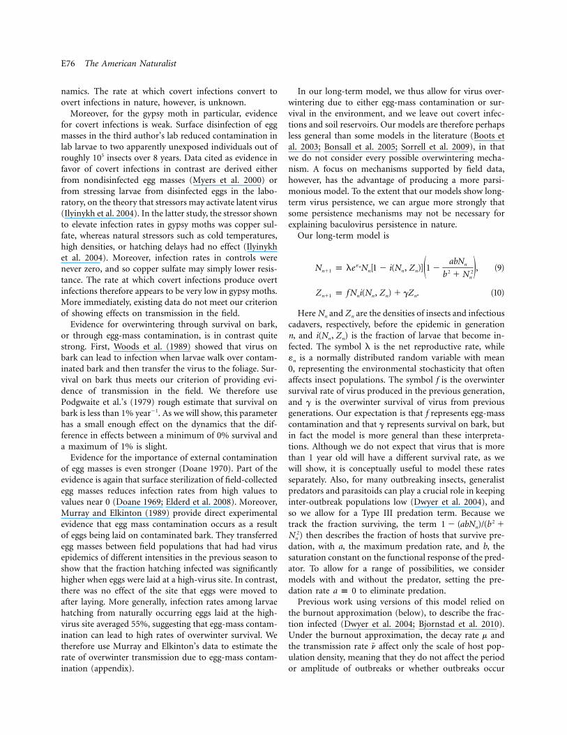
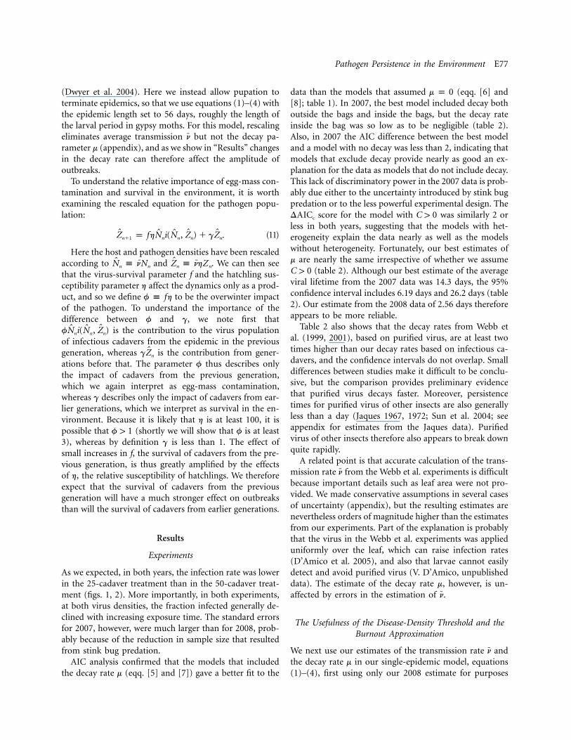
As we expected, in both years, the infection rate was lowerin the 25-cadaver treatment than in the 50-cadaver treat-ment (figs. 1, 2). More importantly, in both experiments,at both virus densities, the fraction infected generally de-clined with increasing exposure time. The standard errorsfor 2007, however, were much larger than for 2008, prob-ably because of the reduction in sample size that resultedfrom stink bug predation.

AIC analysis confirmed that the models that includedthe decay rate m (eqq. [5] and [7]) gave a better fit to the

data than the models that assumed (eqq. [6] andm p 0[8]; table 1). In 2007, the best model included decay bothoutside the bags and inside the bags, but the decay rateinside the bag was so low as to be negligible (table 2).Also, in 2007 the AIC difference between the best modeland a model with no decay was less than 2, indicating thatmodels that exclude decay provide nearly as good an ex-planation for the data as models that do not include decay.This lack of discriminatory power in the 2007 data is prob-ably due either to the uncertainty introduced by stink bugpredation or to the less powerful experimental design. The

score for the model with was similarly 2 orDAIC C 1 0c

less in both years, suggesting that the models with het-erogeneity explain the data nearly as well as the modelswithout heterogeneity. Fortunately, our best estimates ofm are nearly the same irrespective of whether we assume

(table 2). Although our best estimate of the averageC 1 0viral lifetime from the 2007 data was 14.3 days, the 95%confidence interval includes 6.19 days and 26.2 days (table2). Our estimate from the 2008 data of 2.56 days thereforeappears to be more reliable.

Table 2 also shows that the decay rates from Webb etal. (1999, 2001), based on purified virus, are at least twotimes higher than our decay rates based on infectious ca-davers, and the confidence intervals do not overlap. Smalldifferences between studies make it difficult to be conclu-sive, but the comparison provides preliminary evidencethat purified virus decays faster. Moreover, persistencetimes for purified virus of other insects are also generallyless than a day (Jaques 1967, 1972; Sun et al. 2004; seeappendix for estimates from the Jaques data). Purifiedvirus of other insects therefore also appears to break downquite rapidly.

A related point is that accurate calculation of the trans-mission rate from the Webb et al. experiments is difficultn

because important details such as leaf area were not pro-vided. We made conservative assumptions in several casesof uncertainty (appendix), but the resulting estimates arenevertheless orders of magnitude higher than the estimatesfrom our experiments. Part of the explanation is probablythat the virus in the Webb et al. experiments was applieduniformly over the leaf, which can raise infection rates(D’Amico et al. 2005), and also that larvae cannot easilydetect and avoid purified virus (V. D’Amico, unpublisheddata). The estimate of the decay rate m, however, is un-affected by errors in the estimation of .n

The Usefulness of the Disease-Density Threshold and theBurnout Approximation

We next use our estimates of the transmission rate andn

the decay rate m in our single-epidemic model, equations(1)–(4), first using only our 2008 estimate for purposes

E78 The American Naturalist

Figure 1: Comparison of best-fit model prediction to data from 2007. Data (points) show the mean fraction infected, with one standarderror of the mean. Curves show the best-fit model predictions, such that the thin line is for , equation (7), and the thick line is form 1 0

, equation (8). A, Results for 25 cadavers per branch; B, results for 50 cadavers per branch. To illustrate the fit of the models, wem p 0use different vertical axis scales for the two panels.

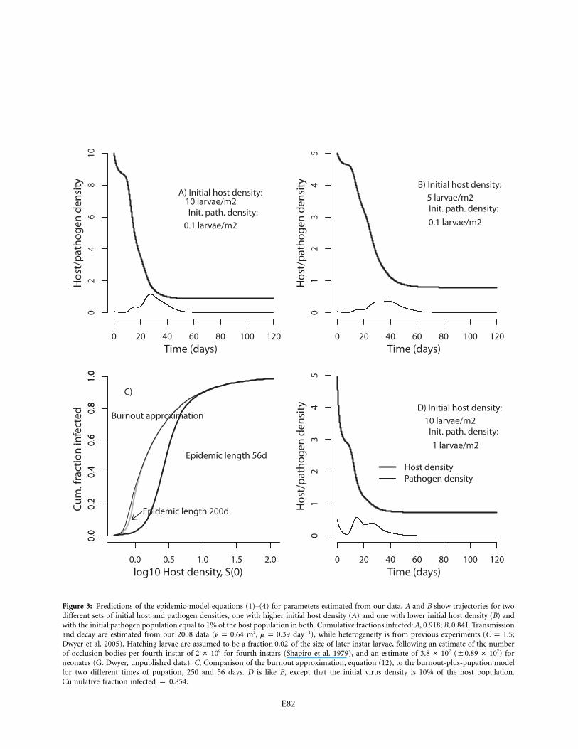
of exposition but shortly considering a range of values. Asfigure 3A, 3B shows, the pathogen begins at a low density,but ultimately it reaches a high enough density to causethe density of uninfected hosts S to drop rapidly (thecomplex fluctuations in the pathogen population reflectthe time delay between infection and death, which intro-duces a kind of stage structure into the infected population(not shown)). Eventually depletion of the susceptible pop-ulation causes viral decay to outweigh transmission, sothat the density of cadavers drops toward zero, leavingbehind a reduced but nonzero host population.

In figure 3A, 3B, the initial host densities are typical ofthe low end of densities at which baculovirus epidemicshave been observed (Woods and Elkinton 1987). Thesepopulations are nevertheless far enough above the disease-density threshold that overall mortality is quite high. It ispossible to prove, however, that the host population in themodel will never reach 0, even if the population starts yetfarther above the threshold and time goes to infinity(Thieme 2003). In the absence of pupation, epidemics inthe model are thus terminated when the infected popu-

lation reaches 0, rather than because there are no moreuninfected hosts, which is the phenomenon known as ep-idemic burnout (Keeling and Rohani 2007).

The fraction of hosts i that remain uninfected afterburnout can be calculated from the implicit equation(Dwyer et al. 2000; Thieme 2003):

2�1/C

¯Cn1 � i p 1 � (S(0)i � P(0)) . (12)[ ]m

Mathematically, this result requires that we allow t r

, but as the trajectories in 3A, 3B indicate, in most cases�the epidemic is over for . In figure 3B, for example,t K �the epidemic is effectively over by days. For gypsyt p 80moths and other outbreaking insects, however, larval pe-riods are typically much less than 80 days (Moreau andLucarotti 2007). It therefore seemed likely that the burnoutapproximation would provide only a rough description ofepidemic severity in these insects.

To show the effect of epidemic length on the accuracyof the burnout approximation, in figure 3C we plot the

Pathogen Persistence in the Environment E79

Figure 2: Comparison of best-fit model prediction to data from 2008. Points and lines are as in figure 1, and again the vertical axis scalesare different for the two panels. A, Results for 25 cadavers per branch; B, results for 50 cadavers per branch.

cumulative fraction infected i versus host density. Figure3C also shows the corresponding predictions of equations(1)–(4), assuming that the epidemic is terminated by pu-pation either at 250 or at 56 days, with the latter valueappropriate for the gypsy moth. The burnout approxi-mation is quite close to the 250-day case, but it is quitefar from the 56-day case. It therefore appears that bothpupation and burnout will limit epidemics, at least at lowvirus densities.

Figure 3C also roughly illustrates the effect of the diseasethreshold, the lowest host density at which a negligibleinitial pathogen density, , produces new infectionsP(0) r 0(Thieme 2003). For equations (1)–(4), the threshold is

, which from our 2008 data is 0.61 larvae m�2. In figure¯m/n3C, a modest number of infections occur below thisthreshold because we have assumed an initial pathogenpopulation equal to 1% of the host population, a valuethat is not that close to 0.

Allowing for both the 2007 and 2008 data, our estimatesof the threshold range from 0.17 to 0.61 larvae m�2 (table2), whereas the lowest density at which an epidemic hasbeen observed in nature is roughly 3 larvae m�2 (Dwyerand Elkinton 1993). Observational studies, however, are

likely to overestimate the population threshold, becausestochastic effects near the threshold will reduce infectionrates (Lloyd-Smith et al. 2005) and because it is difficultto find enough insects to estimate the fraction infected atlow densities (Woods and Elkinton 1987). Moreover, ingypsy moths, host and virus densities are positively cor-related. Indeed, at the lowest density at which an epidemichas been observed in nature, the cumulative infection ratewas higher than 0.2 even though the initial infection ratewas low, suggesting that such populations are well abovethe threshold (Woods et al. 1991). We therefore suspectthat our best threshold estimate of 0.61 larvae m�2 is rea-sonably accurate.

In figure 3C, we assumed an initial infection rate of 1%so as not to completely obscure the density threshold, butepidemics in gypsy moth populations typically begin withinitial infection rates of 10% or more (Woods et al. 1991).This is important because increasing the initial infectionrate causes the epidemic to burn out more rapidly (fig.3D), reducing the inaccuracy of the burnoutapproximation.

In considering a range of decay rates, we therefore in-stead assume that the initial pathogen population is equal

E80 The American Naturalist

Table 1: Corrected Akaike Information Criterion (AICc) values for the models withand without decay rates

Year,decay? Heterogeneity? In-bag decay?

No. parameters(K) QAICc D QAICc

2007:No No No 1 89.57 .31Yes No No 2 90.07 .81No Yes No 2 91.58 2.32Yes Yes No 3 92.00 .73Yes No Yes 3 89.26 0Yes Yes Yes 4 91.27 2.01

2008:No No ... 1 108.11 43.85Yes No ... 2 64.26 0No Yes ... 2 107.68 43.42Yes Yes ... 3 66.30 2.04

Note: Values for the best model in each year are in boldface. QAICc p quasi-likelihood AIC.

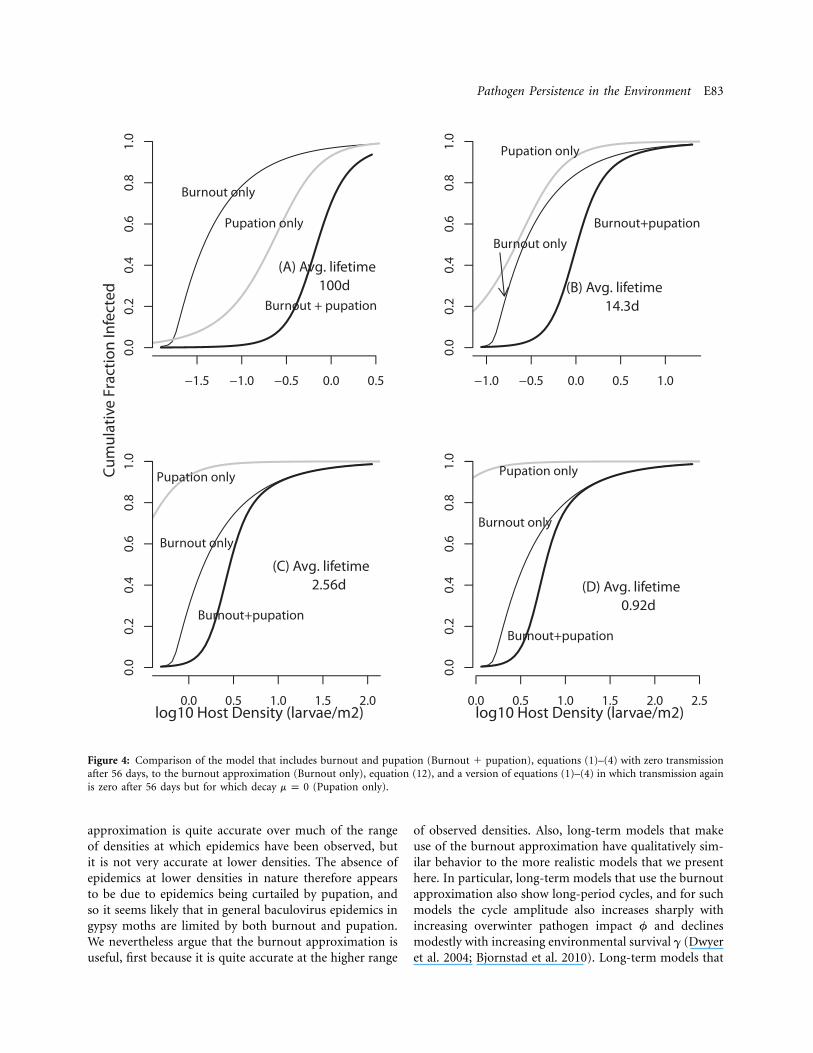
to 10% of the initial host population. In figure 4, we thencompare our model predictions to the prediction of theburnout approximation and to the predictions of a modelin which decay is 0 and transmission is terminated onlyby pupation. In the figure, we use our point estimates ofpersistence from both 2007 (14.3 days) and 2008 (2.56days), as well as an estimate from the Webb et al. (1999)data, and a high value of 100 days to allow for a case ofnear-zero decay. Because the threshold density changeswith the persistence time, for each persistence time we usea range of host densities that is scaled to the threshold,ranging from 0.8 time the threshold to 200 times thethreshold (the panel for 100 days goes to 300# so thatwe can see the full range of infection rates). Woods andElkinton (1987) observed gypsy moth epidemics at hostdensities ranging from 3 to 150 larvae m�2 (0.48–2.2 onthe log10 scale of the graphs), and so only the graph basedon our 2008 estimate (2.56 days, fig. 4C) is centered onthe correct range. For longer persistence times, as for our2007 data (fig. 4B) or for the comparison plot with per-sistence time of 100 days (fig. 4A), the infection rate istoo high at the lower range, while for the shorter persis-tence time of the Webb et al. data (fig. 4D), it is too lowat the higher range. Our estimate of the disease-densitythreshold thus again appears to be reasonably accurate,suggesting that the disease-density threshold is a usefulsummary statistic for understanding epidemics in gypsymoth populations.

To assess the usefulness of the burnout approximation,we consider how it compares to the predictions of therealistic model, which includes both pupation and burn-out. For a persistence time of 100 days, viral decay is lowenough that the realistic model is closest to the pupation-only model, for which , and very far from the burn-m { 0out approximation (fig. 4A). For any shorter persistence

time, as in the estimates based on our data or the Webbet al. (1999) data, the pupation-only model predicts higherinfection rates than the burnout-plus-pupation model orthe burnout approximation. For our best estimate of per-sistence, from the 2008 data, the realistic model closelyapproaches the burnout approximation for densities aboveabout 10 larvae m�2, but it is well below the burnoutapproximation for lower densities (fig. 4C). The burnoutapproximation is therefore reasonably accurate for morethan half the realistic range, but it is quite different fromthe realistic model at lower densities, suggesting that bothpupation and burnout play a role. In particular, pupationis probably part of the reason why epidemics have onlybeen detected at densities considerably higher than thethreshold. The lack of observations of epidemics at lowerdensities may therefore be additional evidence that pu-pation limits epidemics.

Long-Term Dynamics

Figure 5 shows trajectories for the long-term model, in-cluding the host-pathogen-only model that excludes thegeneralist predator and the host-pathogen-predator model.Both models show cycles that qualitatively match cyclesin nature, which typically show a period of 5–10 years andan amplitude of 3–5 orders of magnitude (Elkinton andLiebhold 1990; Johnson et al. 2005). In the host-pathogen-predator model, the generalist predator interacts with sto-chasticity to create variability in outbreak timing and in-tensity (Dwyer et al. 2004).

To see the effects of persistence on outbreak severity,we consider a wider range of persistence times, using theamplitude of fluctuations as a measure of outbreak se-verity. For realistic values of long-term survival g, modestchanges have only slight effects, so we ran the model for

Pathogen Persistence in the Environment E81

Table 2: Best-fit model parameter values for our experiments and for the experiments of Webb et al. (1999, 2001)

Field seasonTransmission n

(m2 day�1)Decay m

(day�1)In-bag decay

(day�1)Heterogeneity

C

Averagepersistence

(days)

Populationthreshold

(insects m�2)

2007 .24 (.17, .32) .04 (10�8, .093) ... ... 25 (10.7, 107) .17 (10�7, .35)2007 .28 (.18, .55) .054 (10�7, .13) ... .56 (10�4, 1.67) 18.5 (7.67, 106) .19 (10�7, .33)2007 .26 (.19, .40) .07 (.03, .11) 10�7 (10�10, .08) ... 14.3 (6.19, 26.6) .27 (.11, .39)2007 .30 (.20, .67) .07 (.04, .16) 10�8 (10�9, .08) .65 (10�4, 1.67) 14.3 (6.19, 26.6) .24 (.11, .36)2008 .64 (.54, .79) .39 (.24, .51) ... ... 2.59 (1.94, 3.95) .61 (.41, .81)2008 .73 (.54, 1.30) .41 (.25, .64) ... .43 (3e-4, .93) 2.43 (1.59, 3.82) .61 (.41, .81)Webb et al. 1999 1,470 (186, 105) 1.09 (.822, 1.67) ... 2.41 (1.95, 3.05) .91 (.60, .91) NAWebb et al. 2001 55.9 (36.3, 110) .92 (.83, 8.47) ... 1.01 (.118, 1.21) 1.47 (1.23, 1.65) NA

Note: Note that the transmission parameters for the Webb et al. data depend on a long list of assumptions and thus are not very reliable (see appendix).

For the Webb et al. data, therefore, we do not include an estimate of the threshold. The upper confidence bound on the decay rate for the Webb et al. (2001)

data is also probably unreliable (appendix). NA p not applicable.

wide ranges of m and f while considering only ,g p 0.01an upper limit based on Podgwaite et al.’s (1979) data,and . We then iterated the models for 200 genera-g p 0tions, long enough to eliminate transients, and we cal-culated the amplitude of fluctuations of host density forthe last 100 generations. We defined the amplitude to bethe difference between the host population density at alocal maximum and the density at the minimum beforethe next maximum, with all densities calculated on a log10

scale. For the host-pathogen-predator model, initial con-ditions can have strong effects, and so for that model weaveraged across initial conditions by drawing initial valuesof host and pathogen densities from uniform distributionsthat spanned the range of values encompassed by the at-tractor of each model. We then calculated the average am-plitude across 10 realizations. Using data from Murray andElkinton (1989), we calculated a point estimate and 95%confidence interval on overwinter survival f, and we usedthe confidence interval to bound f (median 7.14, 95%confidence interval 3.53–23.42; see appendix). To boundwithin-season decay m, we used both our 2007 and 2008estimates and the estimate from the Webb et al. (2001)data.

Figure 6 then shows that increasing values of overwinterimpact f dramatically increase amplitudes for both mod-els, as expected, while within-season persistence time

has more complicated effects. For the host-pathogen-1/monly model, increasing persistence time leads to larger am-plitudes, but the effect is much stronger as survival timeincreases beyond 15 days (about 1.2 on the log10 scale ofour plot). Indeed, for sufficiently high survival times, theamplitude of fluctuations is so large that the cycles areunbounded. The effect of within-season survival is thuscounterintuitive, because the model shows that more rapidbreakdown of virus on foliage makes cycle amplitudessmaller. Smaller-amplitude cycles in turn dampen out-breaks, reducing the chance that the virus will become

extinct and reducing the need for high values of long-termsurvival g. For the host-pathogen-predator model, the ef-fect of persistence is similar except that the cycles are neverunbounded. Also, for very long persistence times, the cy-cles are captured by the low-density equilibrium imposedby the generalist predator, leading to smaller-amplitudefluctuations.

Cycles in our models occur when the pathogen has astrong impact on the host for at least 1 year after the hostpopulation has fallen below its peak. Increasing overwinterimpact f therefore leads to larger-amplitude fluctuationsbecause increasing f increases the severity of the epidemicin the year following the peak (Dwyer et al. 2000). Re-ducing the decay rate m also increases the severity of theepidemic in the year following the peak, because as figure4 shows, reducing m leads to more severe epidemics at lowhost densities. The effect of the decay rate m on epidemicsis thus translated into strong effects on long-termdynamics.

In both models, survival of virus from the previousgeneration, as estimated by the parameter f, appears tobe sufficient to prevent the extinction of the virus even iflonger-term survival . In the more realistic host-g p 0pathogen-predator model in particular, the virus persistsfor the entire range of values of overwinter impact f andwithin-season survival m. We therefore argue that covertinfections and soil reservoirs may not be necessary to ex-plain pathogen-driven outbreaks in the gypsy moth, andperhaps in other outbreaking insects as well. This is notto say that covert infections and soil reservoirs never playa role in the dynamics of baculoviruses but instead thatwe may not need to invoke them to explain viruspersistence.

Discussion

Our best estimate of the persistence time of the gypsy mothbaculovirus is less than 3 days. For this value, the burnout

E82

0 20 40 60 80 100 120

02

46

810

Hos

t/pa

thog

en d

ensi

ty

Time (days)

A) Initial host density:10 larvae/m2Init. path. density:

0.1 larvae/m2

0 20 40 60 80 100 120

01

23

45

Hos

t/pa

thog

en d

ensi

ty

Time (days)

B) Initial host density:5 larvae/m2Init. path. density:

0.1 larvae/m2

0.0

0.2

0.4

0.6

0.8

1.0

0.0

0.2

0.4

0.6

0.8

1.0

0.0 0.5 1.0 1.5 2.0

Cum

. fra

ctio

n in

fect

ed

log10 Host density, S(0)

Epidemic length 56d

Epidemic length 200d

Burnout approximation

C)

0 20 40 60 80 100 120

01

23

45

Hos

t/pa

thog

en d

ensi

ty

Time (days)

Host densityPathogen density

D) Initial host density:10 larvae/m2

Init. path. density:

1 larvae/m2

Figure 3: Predictions of the epidemic-model equations (1)–(4) for parameters estimated from our data. A and B show trajectories for twodifferent sets of initial host and pathogen densities, one with higher initial host density (A) and one with lower initial host density (B) andwith the initial pathogen population equal to 1% of the host population in both. Cumulative fractions infected: A, 0.918; B, 0.841. Transmissionand decay are estimated from our 2008 data ( m2, day�1), while heterogeneity is from previous experiments ( ;n p 0.64 m p 0.39 C p 1.5Dwyer et al. 2005). Hatching larvae are assumed to be a fraction of the size of later instar larvae, following an estimate of the number0.02of occlusion bodies per fourth instar of for fourth instars (Shapiro et al. 1979), and an estimate of ( ) for9 7 72 # 10 3.8 # 10 �0.89 # 10neonates (G. Dwyer, unpublished data). C, Comparison of the burnout approximation, equation (12), to the burnout-plus-pupation modelfor two different times of pupation, 250 and 56 days. D is like B, except that the initial virus density is 10% of the host population.Cumulative fraction infected p 0.854.

Pathogen Persistence in the Environment E83

Figure 4: Comparison of the model that includes burnout and pupation (Burnout � pupation), equations (1)–(4) with zero transmissionafter 56 days, to the burnout approximation (Burnout only), equation (12), and a version of equations (1)–(4) in which transmission againis zero after 56 days but for which decay (Pupation only).m p 0

approximation is quite accurate over much of the rangeof densities at which epidemics have been observed, butit is not very accurate at lower densities. The absence ofepidemics at lower densities in nature therefore appearsto be due to epidemics being curtailed by pupation, andso it seems likely that in general baculovirus epidemics ingypsy moths are limited by both burnout and pupation.We nevertheless argue that the burnout approximation isuseful, first because it is quite accurate at the higher range

of observed densities. Also, long-term models that makeuse of the burnout approximation have qualitatively sim-ilar behavior to the more realistic models that we presenthere. In particular, long-term models that use the burnoutapproximation also show long-period cycles, and for suchmodels the cycle amplitude also increases sharply withincreasing overwinter pathogen impact f and declinesmodestly with increasing environmental survival g (Dwyeret al. 2004; Bjornstad et al. 2010). Long-term models that

E84 The American Naturalist

Host−Pathogen−Only Model

Time (generations)

log1

0 H

ost D

ensi

ty

log1

0 Pa

thog

en D

ensi

ty

0 10 20 30 40 50

−2

−1

01

2

−2

−1

01

2

Host−Pathogen−Predator Model

Time (generations)

Log1

0 H

ost D

ensi

ty

Log1

0 Pa

thog

en D

ensi

ty0 10 20 30 40 50

−2

−1

01

23

−2

−1

01

23

HostPathogen

Figure 5: Trajectories of the long-term model, equations (9), (10). Here the estimate of the decay rate is , from our 2008 data,m p 0.39and the overwinter impact parameter , well within the 95% confidence interval for this parameter. Also, we assume that the epidemicf p 15lasts 2 mo (56 days) after the infected neonates have died. For the host-pathogen-only model, we set predation . For the host-a p 0pathogen-only model, the remaining parameters are taken from Dwyer et al. (2000): reproductive rate , and heterogeneityl p 5.5 C p

. For the host-pathogen-predator model, the remaining parameters are taken from Dwyer et al. (2004): , ,0.86 l p 74.6 a p 0.967 C p, and larvae m2.0.97 b p 0.14

make use of the burnout approximation are therefore qual-itatively useful, especially because they can be understoodmore easily (Dwyer et al. 2000).

The prediction of the host-density threshold is also quiteuseful. We expect that epidemics in nature will occur at hostdensities higher than our best estimate of 0.61 larvae m�2,

and indeed epidemics are typically observed at densitiesabove 3 larvae m�2 (Woods and Elkinton 1987; Woods etal. 1991). An interesting feature of this prediction, however,is that it suggests that insecticidal sprays may be used tobegin epizootics in gypsy moth populations at densities thatare well below outbreak densities (Elkinton and Liebhold

Pathogen Persistence in the Environment E85

0.0 0.5 1.0 1.5

510

1520

Ove

r−w

inte

r im

pact

ϕH

ost−

path

ogen

−on

ly m

odel

Webb’99 2008 2007

Envt’l persistence γ = 0.00

0.0 0.5 1.0 1.5

510

1520

Webb’99 2008 2007

Envt’l persistence γ = 0.01

0.0 0.5 1.0 1.5

510

1520

Foliage persistence 1/µ ,days (log10)

Ove

r−w

inte

r im

pact

ϕH

ost−

path

ogen

−pr

edat

or m

odel

Webb’99 2008 2007

0.0 0.5 1.0 1.5

510

1520

Foliage persistence 1/µ ,days (log10)

Webb’99 2008 2007

Figure 6: Effects of virus persistence parameters on outbreak severity. Other parameters are as in figure 5. Shading indicates amplitudesof fluctuations, such that the darkest represents an amplitude of zero and the lightest represents an amplitude of 7 orders of magnitude.The upper two plots are for the host-pathogen-only model, and the lower two plots are for the host-pathogen-predator model. For thetwo panels on the left, the environmental survival parameter , while for the two on the right, . The error bars on the pointsg p 0 g p 0.01represent the 95% confidence interval on f in the vertical direction, calculated from Murray and Elkinton (1989), and on persistence time

in the horizontal direction, with data sources for m as labeled. For the host-pathogen-only model, periods greater than 6 generally lead1/mto unstable oscillations, in which the virus becomes extinct, but for the host-pathogen-predator model the virus always persists.

1990). More generally, our experimental procedure may beuseful in the further development of the virus as a man-agement tool (Reardon et al. 1996). One of the obstaclesto the development and use of viral sprays is the large-scalefield trials necessary to evaluate transmission efficacy of

different candidate strains (Reardon et al. 1996; Thorpe etal. 1999). Small-scale transmission experiments might re-duce the cost of these evaluations by providing a preliminaryscreening of virus strains. It is important to emphasize,however, that using ground-up cadavers instead of purified

E86 The American Naturalist

virus is unlikely to be a viable strategy in biological control,because of regulations about the content of sprays (Hunter-Fujita et al. 1998).

Because the virus in our long-term models survives in-definitely even if we allow only for persistence of virusfrom the previous generation, we argue that covert infec-tions and soil reservoirs may not be needed to explainbaculovirus dynamics. As we have described, however, evi-dence for covert infections in the lab is stronger for atleast a few other insects (Burden et al. 2003, 2006; Kouassiet al. 2009; Vilaplana et al. 2010) than it is for the gypsymoth (Myers et al. 2000; Ilyinykh et al. 2004), and so thisconclusion may not be general. An additional caveat isthat our models assume that spatial structure plays littlerole. For gypsy moths in North America, this may not bea bad assumption, because regional weather patterns syn-chronize populations over large spatial areas (Peltonen etal. 2002), and allowing for regional weather leads to re-alistic levels of synchrony in spatial versions of our models(Abbott and Dwyer 2008). Nevertheless, in 2001–2003, thethird author observed a postoutbreak gypsy moth popu-lation that persisted at a high density over a small area,within which virus transmission continued for three larvalseasons after the regional population had crashed (G.Dwyer, unpublished data). A deeper understanding oflong-term persistence may therefore require field studiesof the importance of spatial structure in populations atvery low densities.

Nothing about our single-epidemic model is specific tothe gypsy moth–baculovirus interaction, to the extent thatsimilar models are used to describe epidemics of humandiseases (Keeling and Rohani 2007). More concretely, workin the third author’s lab (G. Dwyer et al., unpublisheddata) has shown that the epidemic model provides anexcellent fit to data on baculovirus epidemics in the Doug-las-fir tussock moth (Shepherd et al. 1984; Otvos et al.1987), the western tent caterpillar (Beisner and Myers1999), and the balsam-fir sawfly (Moreau et al. 2005). Ittherefore seems likely that baculovirus epidemics in otheroutbreaking insects are also limited by pupation. The long-term models are similarly not specific to the gypsy moth,in that most outbreaking insects have discrete generationsand transmission in larvae only (Hunter 1991; Dwyer etal. 2004), as assumed by the models. We therefore arguethat egg-mass contamination and environmental survivalare likely to be sufficient to explain virus persistence inother insects as well.

A general conclusion of our work is thus that, whendata are collected in the laboratory or under other artificialconditions, the resulting conclusions may not apply totransmission in nature (Dwyer et al. 2005). The signifi-cantly higher decay rate of purified virus (table 2) em-phasizes this point. A corollary is that estimation of model

parameters from field data can provide useful insights intohost-pathogen dynamics, suggesting that a focus on par-ticular host-pathogen systems can complement the moregeneral models that are typical of most studies in theo-retical ecology. Indeed, tests of theory necessarily requiresystem-specific experiments, and we therefore believe thatour work usefully illustrates the tension between generalityand specificity in population biology.

Interest in the effects of environmental persistence onhost-pathogen dynamics has been driven by efforts to un-derstand human diseases such as cholera (Pascual et al.2002; King et al. 2008) and pandemic influenza (Brebanet al. 2009). Recent work has similarly shown that theenvironmental persistence of Metschnikowia pathogens ofDaphnia plays an important role in the dynamics ofMetschnikowia-Daphnia interactions (Hall et al. 2005,2010; Duffy and Sivars-Becker 2007; Duffy et al. 2010).Studies of the environmental persistence of baculovirusesin contrast have a long history (Jaques 1967; Doane 1969),but a lack of estimates of persistence times has hinderedour understanding of how baculovirus persistence affectsbaculovirus dynamics. We therefore hope to have shownthat quantifying persistence times can lead to a deeperunderstanding of disease spread.

Acknowledgments

E.F. was supported by a Research Experiences for Under-graduates fellowship, through the National Science Foun-dation (NSF). B.D.E. and G.D. were supported by NSFgrants to G.D. A. Hunter provided useful comments onthe manuscript, as did two anonymous reviewers. This iscontribution 1599 of the Kellogg Biological Station.

APPENDIX

Statistical and Mathematical Details

First we derive the equations used in our statistical anal-yses. Second, we explain how we analyzed data on virusdecay from previous experiments. Third, we explain howwe scaled transmission rates. Fourth, we present the re-scaling of the long-term host-pathogen model, equations(9), (10).

Statistical Analyses of Transmission Experiments, andViral Decay Inside Bags

In our experiments, the virus is allowed to decay for Tdays before transmission starts. Decay then ceases and

Pathogen Persistence in the Environment E87

there is no further change in the pathogen population. Ifis the density at the end of the decay period, we canP(0)

rewrite equation (1) for the host population as2C

dS S(t)�mT¯p �nSP(0)e . (A1)( )dt S(0)

This equation can be integrated to give the model equationthat we use in our statistical analyses:

ˆS(t) 22 �mT �1/Cˆ¯p (1 � nC P(0)e t) . (A2)S(0)

For the case of no heterogeneity in infection risk, we setin equation (A1):C p 0

dS�mTp �nSP(0)e . (A3)

dt

We again integrate to find

ˆS(t)�mTˆp exp (�nP(0)e t). (A4)

S(0)

So far we have assumed that there is no viral decay insidethe mesh bags. To fit a model with decay inside the bags,we define to be the decay rate inside the bag and tom m1 2

be the decay rate outside the bag. Because there is no ad-dition of virus, equation (4) for the infectious-cadaver pop-ulation becomes

dPp �m P, (A5)1dt

which has solution . We then insert this�m t1P(t) p P(0)esolution into the host equation (1):

2C

dS S(t)�m t �m T1 2¯p �nSP(0)e e , (A6)( )dt S(0)

Integrating and rearranging in terms of the fraction un-infected gives

2�1/Cˆ�m t1ˆS(t) 1 � e

2 �m T2¯p 1 � nC P(0) e . (A7)( )S(0) m1

Estimating the Virus Decay Rate from PreviousExperiments and Estimating an Egg-Mass

Contamination Rate

We first explain why estimating decay rates from experi-ments with only one virus dose is not statistically feasibleusing standard models. For analyzing dose-response ex-periments with baculoviruses, the standard approach is touse logistic regression, which means using a generalizedlinear model with link logit, also known as a logit model,

with the log-transformed dose as the independent variable(Morgan 1992). To allow for virus decay, we therefore usea logit model, except that we multiply the dose by anexponential decay term:

1p p . (A8)i, j �mtj1 � exp [�b � b log (D e )]0 1 10 i

Here is the probability of infection at dose at timep Di, j i

after the application of the virus, and are parameterst b bj 0 1

describing the increase in the infection rate with increasingdose, and m is again the decay rate of the virus. In usingthe phrase “standard model,” we therefore mean that webegan with a model that is usually used to analyze labo-ratory dose-response transmission experiments, and thenwe extended it to allow for virus decay.

It turns out, however, that we cannot estimate in-b1

dependently of m in this model because of a problemknown in statistics as “nonidentifiability.” To show this,we first solve for the logit-transform of the data:

pi, j �mtjlog p �b � b log (D e ). (A9)0 1 10 i( )1 � pi, j

We then rearrange the right-hand side to give

pi, jlog p �b � b log D � b mt . (A10)0 1 10 i 1 j( )1 � pi, j

If there is only one dose, then the dose is a constant,, and we can define new parameters ˆD { D b { b �i 0 0

and . We can therefore rewrite theˆb log D b { b m1 10 1 1

model to only include two parameters, and . In short,ˆ ˆb b0 1

if there is only one dose, it is not possible to separatelyestimate and m, even if the exposure time is variedb t1 j

experimentally. Note that Sun et al. (2004) avoided thisproblem by estimating and from laboratory dose-b b0 1

response data, and then back-calculating from the fractioninfected in their data to estimate viral population densitiesin the field. It appears to be the case, however, that theyused only the point estimates of and in their cal-b b0 1

culations of viral population densities. If so, the standarderrors on their estimates of viral half-lives (Sun et al. 2004,p. 190, their table 1) are probably underestimates.

The underlying problem is the log-transformed doseterm. Although log transformation allows a better fit tobaculovirus dose-response data, to our knowledge there isno mechanistic explanation for why this is so. This isrelevant because although a different model might nothave this problem, without a deeper understanding of themechanisms underlying the infection process within aninsect, we are in no position to propose a new and bettermodel. The models for our field-transmission experimentsdo not have this problem, but they assume that larvae are

E88 The American Naturalist

allowed to feed at will on foliage in the field, whereas inthe experiments in question, larvae were fed contaminatedfoliage in the laboratory, and larvae that did not consumethe entire dose were discarded. We therefore do not at-tempt to find a better model with which to analyze thistype of data.

We instead restrict ourselves to experiments that usedmultiple doses and multiple exposure times. To our knowl-edge, the available data then include only the experimentsof Jaques (1968, 1972) on the nucleopolyhedrovirus of thecabbage looper Trichoplusia ni, feeding on cabbage, andexperiments by Webb et al. (1999, 2001) on the nucleo-polyhedrovirus of the gypsy moth, feeding on oaks (Quer-cus species). As we mentioned, in all these experimentsthe virus was added to the foliage in the form of a sprayof purified virus. Analyses of the data, whether verbal inthe earlier Jaques’ studies, or statistical in the Webb et al.studies, then focus on the effects of dosage (Jaques 1968)or on the effects of adding different compounds to thevirus spray, such as yeast (Jaques 1972), the optical bright-ener blankophor BBH (Webb et al. 1999), or a virus ofanother insect (Webb et al. 2001). Because we are inter-ested in comparisons to natural decay, in reanalyzing thesedata, we use only data based on either virus in water(Jaques data) or virus in water plus 2% bond sticker (Webbet al. data).

In the Jaques studies, the data are simple fractions ofthe number of larvae exposed to the virus, and so weassumed a binomial likelihood function (McCullagh andNelder 1989). We then fit the parameters , , and m tob b0 1

the data using maximum likelihood, using the nonlinearsearch routine optim in the R programming language tofind the best parameters (R Development Core Team2009). The best-fit versions of the model are shown foreach data set in figure A1. As the figure shows, in generalthe model does a reasonable job of reproducing the data,but calculation of a variance-inflation factor indicates thatthere is a systematic lack of fit (variance inflation 14) inthree of four cases. Visual inspection of the fit of the modelto the data, however, does not reveal any obvious or sys-tematic discrepancies, and so in the absence of furtherknowledge, tweaking the model to improve the fit seemsill advised. We therefore simply report the best-fit param-eter values and the variance-inflation factors (table A1).Note that the persistence times are lower than our esti-mates for the gypsy moth virus, but it is impossible to saywhether this is due to differences in the host-virus systemor to the use of purified virus.

For the Webb et al. data, larvae were allowed to feedon virus-contaminated foliage in the field, as in our ex-periments. We therefore again used the field-transmissionequation (7) to analyze the data. In this case, however, thedata consist of the mean and the standard error of the

fraction infected, calculated over replicates, with each rep-licate equal to a branch (1999, eight replicates; 2001, 10replicates). For the 2001 data in particular, the data areanalyzed in such a way that treatment-specific standarderrors are only reported for the highest of the three virusdensities. Trying a range of standard errors for the lowerdensities suggested that the upper confidence bound onthe decay rate is very sensitive to these standard errors,even though the lower confidence bound is not, so ingeneral we focus on the 1999 data.

Because we do not have the original data, we calculateda likelihood score for each parameter set by integratingover the variance in the data, as represented by the re-ported standard errors. The idea behind this approach isthat we treat the variance in the data as a nuisance pa-rameter, which we eliminate using integration (Berger etal. 1999). Conceptually, the integral can be written as

L(v) p L(v, x)f(x)dx, (A11)�where L is the likelihood, v is a vector of model parameters,x is the data, and is the probability density functionf(x)of the data. In practice, we cannot directly solve this in-tegral, but we can approximate it numerically by drawingsamples from the probability density function of the dataand calculating the average likelihood across samples. Fora large enough sample, this average likelihood will closelyapproximate the integral (Ross 2002).

To explain how we carried out this procedure, we definer to be the number of replicates in each treatment in theexperiment. We then first drew r values of the fractioninfected for each treatment from a normal distributionwith the same mean and standard deviation as the datafor that treatment, and we calculated the mean and thestandard error for this sample. In general, the standarderrors were small enough that we almost never drew neg-ative values, except for a few cases which we set to 10�10,but increasing this latter number to 10�3 had negligibleeffects. Using a lognormal distribution in contrast led tovery large confidence bounds. A complete sample thenconsisted of a set of treatment-specific means and standarderrors. We then drew 25 new samples using these calculatedmeans and standard errors, and we fit the model to the25 samples. Repeating this process 500 times gave us adistribution of values for each parameter, from which wecalculated a median and 95% confidence interval for eachparameter. As with the Jaques (1967, 1972) data, we cal-culated variance inflation factors to assess the goodness offit of the model (Burnham and Anderson 2002). Doingso meant multiplying the number of insects per sample(10 in all cases) times the fraction infected for each boot-strapped sample. The variance inflation factor was less than

Pathogen Persistence in the Environment E89

1 for every sample for the 1999 data, and figure A2 con-firms that the model provides a reasonable fit to each dataset. For the 1999 data, we also fit a model with hetero-geneity , but its AIC score was 60 units larger, soC p 0we report only the results for the model with .C 1 0

To estimate the overwintering parameter f, we basicallyperformed the same procedure, using the data of Murrayand Elkinton (1989). These data give the fraction of larvaehatching infected from eggs laid at sites with differentinfectious-cadaver densities. Because the data include es-timates of the virus densities, it is possible to estimate therate of increase of the fraction infected with virus density.We can then use the data to estimate the overwinteringimpact parameter f, which replaces in equation (A3).�mTneNote that f thus includes both hatchling susceptibility andvirus survival over the winter. A crucial point is that, foreach bootstrapped sample, we drew values both for thefraction of larvae infected, the dependent variable, and forthe density of virus, the independent variable. Figure A3shows the data and the best-fit version of the model. Thehigh uncertainty in the virus density, as indicated by thelarge horizontal error bars on the higher density, probablymakes the largest contribution to the large confidence in-terval on f. Reassuringly, however, again the variance-inflation factor was less than 1 for all samples. Also, amodel with no host heterogeneity, such that , ex-C p 0plained the data much more poorly than did the modelthat assumed , with a difference in AIC scores forC 1 0the two models of 35.

Scaling Transmission Rates. To accurately calculate the dis-ease-density threshold, we must properly scale the trans-mission parameter . To begin with, this means allowingn

for the average area of a leaf, which we take to bem2 based on an earlier study with the same�35.54 # 10

methodology using trees in the same patch of forest(Dwyer et al. 2005). In addition, in the single-epidemicmodel equations (1)–(4), cadaver density is defined interms of fourth-instar cadavers. Because we used neonatecadavers in our experiments, we converted the hatchlingcadaver density into the equivalent fourth-instar cadaverdensity by multiplying the cadaver density by , the0.002ratio of the number of occlusion bodies in first (G. Dwyer,unpublished data; also see the legend for fig. 3 in the maintext) versus fourth-instar cadavers (Shapiro et al. 1979).

Carrying out the equivalent scaling for the Webb et al.(1999, 2001) data is more difficult, because important de-tails are not listed in the original articles. In particular, wedo not know the leaf area in a bag, nor do we know theamount of virus solution sprayed on the leaves. Becausethe experiments are described as being motivated by ex-periments of D’Amico and Elkinton (1995) that were sim-ilar in methodology to our experiments, we assumed the

same leaf area per bag. Because the leaves were sprayeduntil the solution was running off the leaves, we assumedthat the amount of virus solution sprayed was 500 mL.The roughness of these guesses, however, suggests that ourestimates of transmission from the Webb et al. data aren

unreliable.

Rescaling the Multi-Generation Model. Here we rescale themulti-generation model. For convenience, we show themodel again. First, the epidemic model is

2C

dS S(t)¯p � nSP , (A12)( )dt S(0)

2C

dE S(t)1 ¯p nSP � mdE , (A13)1( )dt S(0)

dEi p mdE � mdE (i p 2, … , m), (A14)i�1 idt

dPp mdE � mP. (A15)mdt

The long-term model is

abNnN p lN (1 � i(N , Z )) 1 � , (A16)n�1 n n n 2 2( )b � Nn

Z p f N i(N , Z ) � gZ . (A17)n�1 n n n n

To connect the two models, we set the initial densities ofhosts and cadavers to be

S(0) p N , (A18)n

P(0) p hZ , (A19)n

where h allows for the higher susceptibility of hatchinglarvae, which die and produce infectious cadavers that startthe epidemic (Dwyer et al. 2000). We next define the frac-tion infected in the epidemic as

S(T)i(N , Z ) p 1 � . (A20)n n Nn

Here is the density of uninfected hosts at the end ofS(T)the epidemic, so that T is the duration of the epidemic.

To rescale these equations, we multiply almost all thestate variables by the transmission rate , except that wen

multiply the infectious-cadaver population by :¯Z hnn

ˆ ˆ ˆ¯ ¯ ¯S { nS(t), E { nE (t), P { nP(t), (A21)i i

ˆˆ ¯ ¯N { nN , Z { nhZ (A22)n n n n

ˆ ¯f { fh, b { bn. (A23)

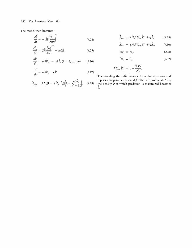
E90 The American Naturalist

The model then becomes2C

ˆ ˆdS S(t)ˆ ˆp � SP , (A24)( )ˆdt S(0)2C

ˆˆdE S(t)1 ˆ ˆ ˆp SP � mdE , (A25)1( )ˆdt S(0)

ˆdEi ˆ ˆp mdE � mdE (i p 2, … , m), (A26)i�1 idt

ˆdP ˆ ˆp mdE � mP. (A27)mdt

ˆ ˆabNnˆˆ ˆ ˆN p lN (1 � i(N , Z )) 1 � , (A28)n�1 n n n 2 2ˆ( )ˆb � Nn

ˆ ˆ ˆˆ ˆZ p fN i(N , Z ) � gZ . (A29)n�1 n n n n

ˆ ˆ ˆˆ ˆZ p fN i(N , Z ) � gZ . (A30)n�1 n n n n

ˆ ˆS(0) p N , (A31)n

ˆP(0) p Z , (A32)n

S(T)ˆˆi(N , Z ) p 1 � .n n Nn

The rescaling thus eliminates from the equations andn

replaces the parameters h and f with their product f. Also,the density b at which predation is maximized becomes

.b

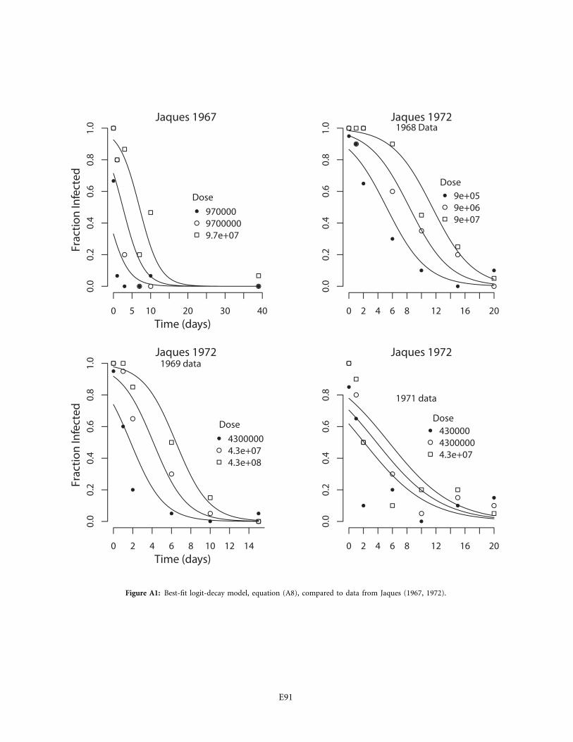
E91

Figure A1: Best-fit logit-decay model, equation (A8), compared to data from Jaques (1967, 1972).

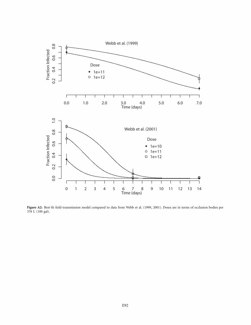
E92

0.0 1.0 2.0 3.0 4.0 5.0 6.0 7.0Time (days)

0.2

0.4

0.6

0.8

Frac

tion

Infe

cted

Webb et al. (1999)

Dose

1e+111e+12

0 1 2 3 4 5 6 7 8 9 10 11 12 13 14Time (days)

0.0

0.2

0.4

0.6

0.8

1.0

Frac

tion

Infe

cted

Webb et al. (2001)

Dose

1e+101e+111e+12

Figure A2: Best-fit field-transmission model compared to data from Webb et al. (1999, 2001). Doses are in terms of occlusion bodies per378 L (100 gal).

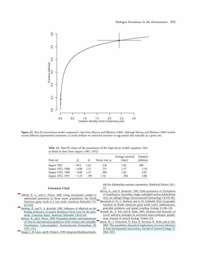
Pathogen Persistence in the Environment E93

Cadaver density (/m2) in previous year

Frac

tion

infe

cted

0.0 0.5 1.0 1.5 2.0 2.5 3.0

0.0

0.1

0.2

0.3

0.4

0.5

0.6

Figure A3: Best-fit transmission model compared to data from Murray and Elkinton (1989). Although Murray and Elkinton (1989) includeseveral different experimental treatments, to avoid artifacts we restricted ourselves to egg masses laid naturally at a given site.

Table A1: Best-fit values of the parameters of the logit-decay model, equation (A8),as fitted to data from Jaques (1967, 1972)

Data set b0 b1 Decay rate m

Average survival(days)

Varianceinflation

Jaques 1967 �10.4 1.62 .516 1.94 488Jaques 1972, 1968 �4.88 1.13 .731 1.37 3.10Jaques 1972, 1969 �8.04 1.37 .984 1.02 8.87Jaques 1972, 1971 �1.73 .391 1.34 .746 5.08

Literature Cited

Abbott, K. C., and G. Dwyer. 2008. Using mechanistic models tounderstand synchrony in forest insect populations: the NorthAmerican gypsy moth as a case study. American Naturalist 172:613–624.

Barbosa, P., and V. A. Krischik. 1987. Influence of alkaloids on thefeeding preference of eastern deciduous forest trees by the gypsymoth, Lymantria dispar. American Naturalist 130:53–69.

Beisner, B., and J. Myers. 1999. Population density and transmissionof virus in experimental populations of the western tent caterpillar(Lepidoptera: Lasiocampidae). Environmental Entomology 28:1107–1113.

Berger, J., B. Liseo, and R. Wolpert. 1999. Integrated likelihood meth-

ods for eliminating nuisance parameters. Statistical Science 14:1–22.

Biever, K., and D. Hostetter. 1985. Field persistence of Trichoplusiani (Lepidoptera, Noctuidae) single-embedded nuclear polyhedrosisvirus on cabbage foliage. Environmental Entomology 14:579–581.

Bjornstad, O. N., C. Robinet, and A. M. Liebhold. 2010. Geographicvariation in North American gypsy moth cycles: subharmonics,generalist predators, and spatial coupling. Ecology 91:106–118.

Bonsall, M., S. Sait, and R. Hails. 2005. Invasion and dynamics ofcovert infection strategies in structured insect-pathogen popula-tions. Journal of Animal Ecology 74:464–474.

Boots, M., J. Greenman, D. Ross, R. Norman, R. Hails, and S. Sait.2003. The population dynamical implications of covert infectionsin host-microparasite interactions. Journal of Animal Ecology 72:1064–1072.

E94 The American Naturalist

Breban, R., J. M. Drake, D. E. Stallknecht, and P. Rohani. 2009. Therole of environmental transmission in recurrent avian influenzaepidemics. PLoS Computational Biology 5:e1000346. doi:10.1371/journal.pcbi.1000346.

Broome, J. R., P. P. Sikorowski, and W. W. Neel. 1974. Effect ofsunlight on activity of nuclear polyhedrosis virus from Malacosomadisstria. Journal of Economic Entomology 67:135–136.

Burden, J., C. Nixon, A. Hodgkinson, R. Possee, S. Sait, L. King, andR. Hails. 2003. Covert infections as a mechanism for long-termpersistence of baculoviruses. Ecology Letters 6:524–531.

Burden, J., R. Possee, S. Sait, L. King, and R. Hails. 2006. Phenotypicand genotypic characterisation of persistent baculovirus infectionsin populations of the cabbage moth (Mamestra brassicae) withinthe British Isles. Archives of Virology 151:635–649.

Burnham, K. P., and D. R. Anderson. 2002. Model selection andmultimodel inference: a practical information-theoretic approach.2nd ed. Springer New York.

Capinera, J. L., S. P. Kirouac, and P. Barbosa. 1976. Phagodeterrencyof cadaver components to gypsy moth larvae, Lymantria dispar.Journal of Invertebrate Pathology 28:277–279.

Cory, J. S., and J. H. Myers. 2003. The ecology and evolution ofinsect baculoviruses. Annual Review of Ecological and Evolution-ary Systems 34:239–272.

D’Amico, V., and J. S. Elkinton. 1995. Rainfall effects on transmissionof gypsy moth (Lepidoptera, Lymantriidae) nuclear polyhedrosisvirus. Environmental Entomology 24:1144–1149.

D’Amico, V., J. Elkinton, J. Podgwaite, J. Buonaccorsi, and G. Dwyer.2005. Pathogen clumping: an explanation for non-linear trans-mission of an insect virus. Ecological Entomology 30:383–390.

Doane, C. 1969. Trans-ovum transmission of a nuclear-polyhedrosisvirus in gypsy moth and inducement of virus susceptibility. Journalof Invertebrate Pathology 14:199–210.

———. 1970. Primary pathogens and their role in development ofan epizootic in gypsy moth. Journal of Invertebrate Pathology 15:21–33.

Dobson, A., and M. Meagher. 1996. The population dynamics ofbrucellosis in the Yellowstone National Park. Ecology 77:1026–1036.

Duffy, M. A., and L. Sivars-Becker. 2007. Rapid evolution and eco-logical host-parasite dynamics. Ecology Letters 10:44–53.

Duffy, M. A., C. E. Caceres, S. R. Hall, A. J. Tessier, and A. R. Ives.2010. Temporal, spatial, and between-host comparisons of patternsof parasitism in lake zooplankton. Ecology 91:3322–3331.

Dwyer, G. 1991. The effects of density, stage and spatial heterogeneityon the transmission of an insect virus. Ecology 72:559–574.

Dwyer, G., and J. S. Elkinton. 1993. Using simple models to predictvirus epizootics in gypsy moth populations. Journal of AnimalEcology 62:1–11.

Dwyer, G., J. S. Elkinton, and J. P. Buonaccorsi. 1997. Host hetero-geneity in susceptibility and disease dynamics: tests of a mathe-matical model. American Naturalist 150:685–707.

Dwyer, G., J. Dushoff, J. S. Elkinton, and S. A. Levin. 2000. Pathogen-driven outbreaks in forest defoliators revisted: building modelsfrom experimental data. American Naturalist 156:105–120.

Dwyer, G., J. Dushoff, and S. Yee. 2004. The combined effects ofpathogens and predators on insect outbreaks. Nature 430:341–345.

Dwyer, G., J. Firestone, and T. E. Stevens. 2005. Should models ofdisease dynamics in herbivorous insects include the effects of va-ratiability in host-plant foliage quality? American Naturalist 165:16–31.

Ebert, D., O. Rainey, T. M. Embley, and D. Scholz. 1996. Develop-ment, life cycle, ultrastructure and phylogenetic position of Pas-teuria ramosa Metchnikoff 1888: rediscovery of an obligate en-doparasite of Daphnia magna Straus. Philosophical Transactionsof the Royal Society B: Biological Sciences 351:1689–1701.

Efron, B., and R. J. Tibshirani. 1994. An introduction to the boot-strap. Chapman & Hall/CRC, New York.

Elderd, B. D., J. Dushoff, and G. Dwyer. 2008. Host-pathogen in-teractions, insect outbreaks, and natural selection for disease re-sistance. American Naturalist 172:829–842.

Elkinton, J. S., and A. M. Liebhold. 1990. Population dynamics ofgypsy moth in North America. Annual Review of Entomology 35:571–596.

Elnagar, S., and S. Abul-Nasr. 1980. Effect of direct sunlight on thevirulence of NPV (nuclear polyhedrosis-virus) of the cotton leaf-worm, Spodoptera littoralis (boisd). Journal of Applied Entomology90:75–80.

Entwistle, P. F., and P. H. W. Adams. 1977. Prolonged retention ofinfectivity in nuclear polyhedrosis virus of Gilpinia hercyniae (Hy-menoptera, Diprionidae) on foliage of spruce species. Journal ofInvertebrate Pathology 29:392–394.

Fuxa, J. R., and A. R. Richter. 2007. Effect of nucleopolyhedrovirusconcentration in soil on viral transport to cotton (Gossypium hir-sutum L.) plants. Biocontrol 52:821–843.

Georgievska, L., R. S. M. De Vries, P. Gao, X. Sun, J. S. Cory, J. M.Vlak, and W. Van Der Werf. 2010. Transmission of wild-type andrecombinant HaSNPV among larvae of Helicoverpa armigera (Lep-idoptera: Noctuidae) on cotton. Environmental Entomology 39:459–467.

Goulson, D., R. Hails, T. Williams, M. Hirst, S. Vasconcelos, B. Green,T. Carty, and J. Cory. 1995. Transmission dynamics of a virus ina stage-structured insect population. Ecology 76:392–401.

Grove, M. J., and K. Hoover. 2007. Intrastadial developmental re-sistance of third instar gypsy moths (Lymantria dispar L.) to L.dispar nucleopolyhedrovirus. Biological Control 40:355–361.

Hails, R., P. Hernandez-Crespo, S. Sait, C. Donnelly, B. Green, andJ. Cory. 2002. Transmission patterns of natural and recombinantbaculoviruses. Ecology 83:906–916.

Hall, S. R., M. A. Duffy, A. J. Tessier, and C. E. Caceres. 2005. Spatialheterogeneity of daphniid parasitism within lakes. Oecologia (Ber-lin) 143:635–644.

Hall, S. R., C. R. Becker, M. A. Duffy, and C. E. Caceres. 2010.Variation in resource acquisition and use among host clones createskey epidemiological trade-offs. American Naturalist 176:557–565.

Hochberg, M. E. 1989. The potential role of pathogens in biologicalcontrol. Nature 337:262–265.

Hunter, A. 1991. Traits that distinguish outbreaking and nonout-breaking macrolepidoptera feeding on northern hardwood trees.Oikos 60:275–282.

Hunter-Fujita, F., P. Entwistle, H. Evans, and N. Crook. 1998. Insectviruses and pest management. Wiley, Chichester.

Ignoffo, C. M., D. L. Hostetter, P. P. Sikorowski, G. Sutter, and W.M. Brooks. 1977. Inactivation of representative species of ento-mopathogenic viruses, a bacterium, fungus, and protozoan by anUV light-source. Environmental Entomology 6:411–415.

Il’inykh, A., and E. Ul’yanova. 2005. Latency of baculoviruses. BiologyBulletin 32:496–502.

Ilyinykh, A., M. Shternshis, and S. Kuzminov. 2004. Exploration intoa mechanism of transgenerational transmission of nucleopolyhe-

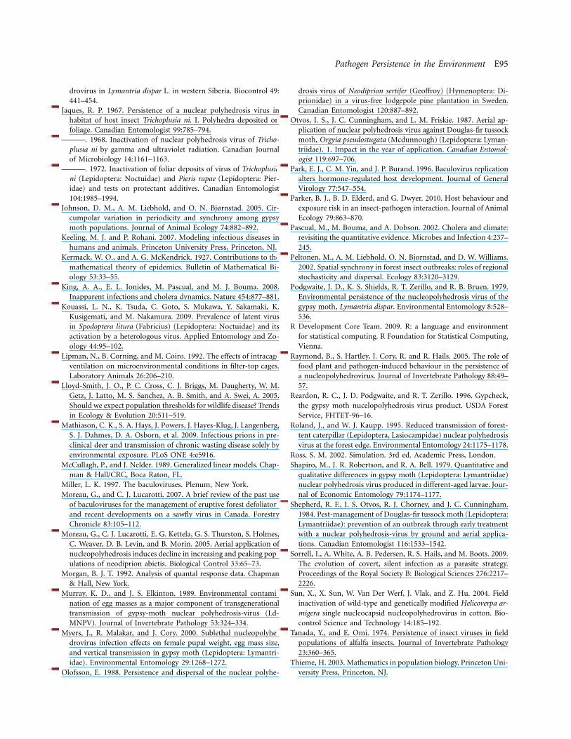
Pathogen Persistence in the Environment E95

drovirus in Lymantria dispar L. in western Siberia. Biocontrol 49:441–454.

Jaques, R. P. 1967. Persistence of a nuclear polyhedrosis virus inhabitat of host insect Trichoplusia ni. I. Polyhedra deposited onfoliage. Canadian Entomologist 99:785–794.

———. 1968. Inactivation of nuclear polyhedrosis virus of Tricho-plusia ni by gamma and ultraviolet radiation. Canadian Journalof Microbiology 14:1161–1163.

———. 1972. Inactivation of foliar deposits of virus of Trichoplusiani (Lepidoptera: Noctuidae) and Pieris rapae (Lepidoptera: Pier-idae) and tests on protectant additives. Canadian Entomologist104:1985–1994.

Johnson, D. M., A. M. Liebhold, and O. N. Bjørnstad. 2005. Cir-cumpolar variation in periodicity and synchrony among gypsymoth populations. Journal of Animal Ecology 74:882–892.

Keeling, M. J. and P. Rohani. 2007. Modeling infectious diseases inhumans and animals. Princeton University Press, Princeton, NJ.

Kermack, W. O., and A. G. McKendrick. 1927. Contributions to themathematical theory of epidemics. Bulletin of Mathematical Bi-ology 53:33–55.

King, A. A., E. L. Ionides, M. Pascual, and M. J. Bouma. 2008.Inapparent infections and cholera dynamics. Nature 454:877–881.

Kouassi, L. N., K. Tsuda, C. Goto, S. Mukawa, Y. Sakamaki, K.Kusigemati, and M. Nakamura. 2009. Prevalence of latent virusin Spodoptera litura (Fabricius) (Lepidoptera: Noctuidae) and itsactivation by a heterologous virus. Applied Entomology and Zo-ology 44:95–102.

Lipman, N., B. Corning, and M. Coiro. 1992. The effects of intracageventilation on microenvironmental conditions in filter-top cages.Laboratory Animals 26:206–210.

Lloyd-Smith, J. O., P. C. Cross, C. J. Briggs, M. Daugherty, W. M.Getz, J. Latto, M. S. Sanchez, A. B. Smith, and A. Swei, A. 2005.Should we expect population thresholds for wildlife disease? Trendsin Ecology & Evolution 20:511–519.

Mathiason, C. K., S. A. Hays, J. Powers, J. Hayes-Klug, J. Langenberg,S. J. Dahmes, D. A. Osborn, et al. 2009. Infectious prions in pre-clinical deer and transmission of chronic wasting disease solely byenvironmental exposure. PLoS ONE 4:e5916.

McCullagh, P., and J. Nelder. 1989. Generalized linear models. Chap-man & Hall/CRC, Boca Raton, FL.

Miller, L. K. 1997. The baculoviruses. Plenum, New York.Moreau, G., and C. J. Lucarotti. 2007. A brief review of the past use

of baculoviruses for the management of eruptive forest defoliatorsand recent developments on a sawfly virus in Canada. ForestryChronicle 83:105–112.

Moreau, G., C. J. Lucarotti, E. G. Kettela, G. S. Thurston, S. Holmes,C. Weaver, D. B. Levin, and B. Morin. 2005. Aerial application ofnucleopolyhedrosis induces decline in increasing and peaking pop-ulations of neodiprion abietis. Biological Control 33:65–73.

Morgan, B. J. T. 1992. Analysis of quantal response data. Chapman& Hall, New York.

Murray, K. D., and J. S. Elkinton. 1989. Environmental contami-nation of egg masses as a major component of transgenerationaltransmission of gypsy-moth nuclear polyhedrosis-virus (Ld-MNPV). Journal of Invertebrate Pathology 53:324–334.

Myers, J., R. Malakar, and J. Cory. 2000. Sublethal nucleopolyhe-drovirus infection effects on female pupal weight, egg mass size,and vertical transmission in gypsy moth (Lepidoptera: Lymantri-idae). Environmental Entomology 29:1268–1272.

Olofsson, E. 1988. Persistence and dispersal of the nuclear polyhe-

drosis virus of Neodiprion sertifer (Geoffroy) (Hymenoptera: Di-prionidae) in a virus-free lodgepole pine plantation in Sweden.Canadian Entomologist 120:887–892.

Otvos, I. S., J. C. Cunningham, and L. M. Friskie. 1987. Aerial ap-plication of nuclear polyhedrosis virus against Douglas-fir tussockmoth, Orgyia pseudostugata (Mcdunnough) (Lepidoptera: Lyman-triidae). 1. Impact in the year of application. Canadian Entomol-ogist 119:697–706.

Park, E. J., C. M. Yin, and J. P. Burand. 1996. Baculovirus replicationalters hormone-regulated host development. Journal of GeneralVirology 77:547–554.

Parker, B. J., B. D. Elderd, and G. Dwyer. 2010. Host behaviour andexposure risk in an insect-pathogen interaction. Journal of AnimalEcology 79:863–870.

Pascual, M., M. Bouma, and A. Dobson. 2002. Cholera and climate:revisiting the quantitative evidence. Microbes and Infection 4:237–245.

Peltonen, M., A. M. Liebhold, O. N. Bjornstad, and D. W. Williams.2002. Spatial synchrony in forest insect outbreaks: roles of regionalstochasticity and dispersal. Ecology 83:3120–3129.

Podgwaite, J. D., K. S. Shields, R. T. Zerillo, and R. B. Bruen. 1979.Environmental persistence of the nucleopolyhedrosis virus of thegypsy moth, Lymantria dispar. Environmental Entomology 8:528–536.

R Development Core Team. 2009. R: a language and environmentfor statistical computing. R Foundation for Statistical Computing,Vienna.

Raymond, B., S. Hartley, J. Cory, R. and R. Hails. 2005. The role offood plant and pathogen-induced behaviour in the persistence ofa nucleopolyhedrovirus. Journal of Invertebrate Pathology 88:49–57.

Reardon, R. C., J. D. Podgwaite, and R. T. Zerillo. 1996. Gypcheck,the gypsy moth nucelopolyhedrosis virus product. USDA ForestService, FHTET-96–16.

Roland, J., and W. J. Kaupp. 1995. Reduced transmission of forest-tent caterpillar (Lepidoptera, Lasiocampidae) nuclear polyhedrosisvirus at the forest edge. Environmental Entomology 24:1175–1178.

Ross, S. M. 2002. Simulation. 3rd ed. Academic Press, London.Shapiro, M., J. R. Robertson, and R. A. Bell. 1979. Quantitative and

qualitative differences in gypsy moth (Lepidoptera: Lymantriidae)nuclear polyhedrosis virus produced in different-aged larvae. Jour-nal of Economic Entomology 79:1174–1177.

Shepherd, R. F., I. S. Otvos, R. J. Chorney, and J. C. Cunningham.1984. Pest-management of Douglas-fir tussock moth (Lepidoptera:Lymantriidae): prevention of an outbreak through early treatmentwith a nuclear polyhedrosis-virus by ground and aerial applica-tions. Canadian Entomologist 116:1533–1542.

Sorrell, I., A. White, A. B. Pedersen, R. S. Hails, and M. Boots. 2009.The evolution of covert, silent infection as a parasite strategy.Proceedings of the Royal Society B: Biological Sciences 276:2217–2226.

Sun, X., X. Sun, W. Van Der Werf, J. Vlak, and Z. Hu. 2004. Fieldinactivation of wild-type and genetically modified Helicoverpa ar-migera single nucleocapsid nucleopolyhedrovirus in cotton. Bio-control Science and Technology 14:185–192.

Tanada, Y., and E. Omi. 1974. Persistence of insect viruses in fieldpopulations of alfalfa insects. Journal of Invertebrate Pathology23:360–365.

Thieme, H. 2003. Mathematics in population biology. Princeton Uni-versity Press, Princeton, NJ.

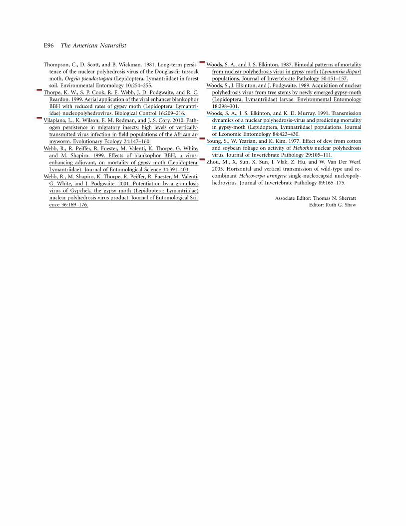
E96 The American Naturalist

Thompson, C., D. Scott, and B. Wickman. 1981. Long-term persis-tence of the nuclear polyhedrosis virus of the Douglas-fir tussockmoth, Orgyia pseudostugata (Lepidoptera, Lymantriidae) in forestsoil. Environmental Entomology 10:254–255.

Thorpe, K. W., S. P. Cook, R. E. Webb, J. D. Podgwaite, and R. C.Reardon. 1999. Aerial application of the viral enhancer blankophorBBH with reduced rates of gypsy moth (Lepidoptera: Lymantri-idae) nucleopolyhedrovirus. Biological Control 16:209–216.

Vilaplana, L., K. Wilson, E. M. Redman, and J. S. Cory. 2010. Path-ogen persistence in migratory insects: high levels of vertically-transmitted virus infection in field populations of the African ar-myworm. Evolutionary Ecology 24:147–160.

Webb, R., R. Peiffer, R. Fuester, M. Valenti, K. Thorpe, G. White,and M. Shapiro. 1999. Effects of blankophor BBH, a virus-enhancing adjuvant, on mortality of gypsy moth (Lepidoptera:Lymantriidae). Journal of Entomological Science 34:391–403.

Webb, R., M. Shapiro, K. Thorpe, R. Peiffer, R. Fuester, M. Valenti,G. White, and J. Podgwaite. 2001. Potentiation by a granulosisvirus of Gypchek, the gypsy moth (Lepidoptera: Lymantriidae)nuclear polyhedrosis virus product. Journal of Entomological Sci-ence 36:169–176.

Woods, S. A., and J. S. Elkinton. 1987. Bimodal patterns of mortalityfrom nuclear polyhedrosis virus in gypsy moth (Lymantria dispar)populations. Journal of Invertebrate Pathology 50:151–157.

Woods, S., J. Elkinton, and J. Podgwaite. 1989. Acquisition of nuclearpolyhedrosis virus from tree stems by newly emerged gypsy-moth(Lepidoptera, Lymantriidae) larvae. Environmental Entomology18:298–301.

Woods, S. A., J. S. Elkinton, and K. D. Murray. 1991. Transmissiondynamics of a nuclear polyhedrosis-virus and predicting mortalityin gypsy-moth (Lepidoptera, Lymnatriidae) populations. Journalof Economic Entomology 84:423–430.

Young, S., W. Yearian, and K. Kim. 1977. Effect of dew from cottonand soybean foliage on activity of Heliothis nuclear polyhedrosisvirus. Journal of Invertebrate Pathology 29:105–111.

Zhou, M., X. Sun, X. Sun, J. Vlak, Z. Hu, and W. Van Der Werf.2005. Horizontal and vertical transmission of wild-type and re-combinant Helicoverpa armigera single-nucleocapsid nucleopoly-hedrovirus. Journal of Invertebrate Pathology 89:165–175.

Associate Editor: Thomas N. SherrattEditor: Ruth G. Shaw