Noname manuscript No. (will be inserted by the editor) Path Representation in Circuit Netlists Using Linear-Sized ZDDs with Optimal Variable Ordering Stelios N. Neophytou and Maria K. Michael Received: 25 Jun 2018 / Accepted: date Abstract The efficient representation and manipula- tion of a large number of paths in a Directed Acyclic Graph (DAG) requires the usage of special data struc- tures that may become of exponential size with respect to the size of the graph. Several methodologies targeting Electronic Design Automation problems such as tim- ing analysis, physical design, verification and testing involve path representation and necessary manipula- tion. Previous works proposed an encoding using Zero- suppressed Binary Decision Diagrams (ZDDs), which has been shown experimentally to cope well when rep- resenting structural or logical paths in VLSI circuits. However, it is well known that the ordering of the vari- ables in a ZDD highly affects its size and, therefore, the efficiency of the methodologies utilizing these data structures. In this work, we show that using a reverse topological order for the ZDD variables bounds the number of nodes in the ZDD representing structural paths to the number of edges in the DAG considered, hence, making the ZDD size linear to the DAG’s size. This result, supported here both theoretically and ex- perimentally, is very important as it can render method- ologies with questionable scalability applicable to larger industrial designs. We demonstrate the applicability of S. N. Neophytou Engineering Dept., University of Nicosia, P.O.Box 24005, CY-1700, Nicosia, Cyprus tel.: +357 22 842518 E-mail: [email protected] Maria K. Michael Electrical and Computer Engineering Dept., and KIOS Research and Innovation Center of Excellence University of Cyprus, Nicosia, Cyprus. tel.: +357 22 892277 E-mail: [email protected] the proposed variable ordering in one such methodol- ogy which utilizes ZDDs to grade the Path Delay Fault coverage of a given test set. Keywords Paths Representation · Binary Decision Diagrams · Path Delay Fault Simulation and Test · Timing Analysis · Timing Verification. 1 Introduction Theoretic approaches that use graphs, mathematical structures representing relationships using vertices and edges [18], have been used to solve problems in a plethora of scientific disciplines. From linguistics to biology and from sociology to software development all kind of prob- lems have been mapped into graphs and solved using graph theoretic algorithms. Problems such as pattern matching for DNA sequences [47], speech recognition [27], data mining [21], identifying dependencies in pro- gramming language compilers [45], finding the optimal route in a communication [9] or transportation [19] net- work, logic synthesis of electronic circuits [12], among others, require path representation and manipulation. A special case of such graphs, with important sig- nificance, is the Directed Acyclic Graph (DAGs) whose edges are unidirectional and no loops are allowed within the structure. While DAGs are restricted graphs, many algorithms have been developed based on them, (or on some variation), finding many applications in science and engineering. A number of problems using DAGs deal with the identification, representation, traversal and/or enumeration of the graph paths. In the gen- eral case, the number of paths in a DAG can be ex- ponential to the number of vertices in the graph As a result, both the data structure used and the algorithms developed should be chosen carefully in order to keep

Welcome message from author
This document is posted to help you gain knowledge. Please leave a comment to let me know what you think about it! Share it to your friends and learn new things together.
Transcript
Noname manuscript No.(will be inserted by the editor)
Path Representation in Circuit Netlists Using Linear-SizedZDDs with Optimal Variable Ordering
Stelios N. Neophytou and Maria K. Michael
Received: 25 Jun 2018 / Accepted: date
Abstract The efficient representation and manipula-
tion of a large number of paths in a Directed Acyclic
Graph (DAG) requires the usage of special data struc-
tures that may become of exponential size with respect
to the size of the graph. Several methodologies targeting
Electronic Design Automation problems such as tim-
ing analysis, physical design, verification and testing
involve path representation and necessary manipula-
tion. Previous works proposed an encoding using Zero-
suppressed Binary Decision Diagrams (ZDDs), which
has been shown experimentally to cope well when rep-
resenting structural or logical paths in VLSI circuits.
However, it is well known that the ordering of the vari-
ables in a ZDD highly affects its size and, therefore,
the efficiency of the methodologies utilizing these data
structures. In this work, we show that using a reversetopological order for the ZDD variables bounds the
number of nodes in the ZDD representing structural
paths to the number of edges in the DAG considered,
hence, making the ZDD size linear to the DAG’s size.
This result, supported here both theoretically and ex-
perimentally, is very important as it can render method-
ologies with questionable scalability applicable to larger
industrial designs. We demonstrate the applicability of
S. N. NeophytouEngineering Dept.,University of Nicosia,P.O.Box 24005, CY-1700, Nicosia, Cyprustel.: +357 22 842518E-mail: [email protected]
Maria K. MichaelElectrical and Computer Engineering Dept., andKIOS Research and Innovation Center of ExcellenceUniversity of Cyprus,Nicosia, Cyprus.tel.: +357 22 892277E-mail: [email protected]
the proposed variable ordering in one such methodol-
ogy which utilizes ZDDs to grade the Path Delay Fault
coverage of a given test set.
Keywords Paths Representation · Binary Decision
Diagrams · Path Delay Fault Simulation and Test ·Timing Analysis · Timing Verification.
1 Introduction
Theoretic approaches that use graphs, mathematical
structures representing relationships using vertices and
edges [18], have been used to solve problems in a plethora
of scientific disciplines. From linguistics to biology and
from sociology to software development all kind of prob-
lems have been mapped into graphs and solved usinggraph theoretic algorithms. Problems such as pattern
matching for DNA sequences [47], speech recognition
[27], data mining [21], identifying dependencies in pro-
gramming language compilers [45], finding the optimal
route in a communication [9] or transportation [19] net-
work, logic synthesis of electronic circuits [12], among
others, require path representation and manipulation.
A special case of such graphs, with important sig-
nificance, is the Directed Acyclic Graph (DAGs) whose
edges are unidirectional and no loops are allowed within
the structure. While DAGs are restricted graphs, many
algorithms have been developed based on them, (or on
some variation), finding many applications in science
and engineering. A number of problems using DAGs
deal with the identification, representation, traversal
and/or enumeration of the graph paths. In the gen-
eral case, the number of paths in a DAG can be ex-
ponential to the number of vertices in the graph As a
result, both the data structure used and the algorithms
developed should be chosen carefully in order to keep
2 Stelios N. Neophytou and Maria K. Michael
the computational effort manageable (i.e., not requiring
prohibitively large memory space). In essence, the po-
tentially large number of paths in, even medium sized
DAGs, does not permit the usage of any kind of path-
enumerative steps in these algorithms.
In traditional VLSI design, DAGs have been exten-
sively used for representing circuit netlists and phys-
ical design layouts In the area of Electronic Design
Automation (EDA) the usage of DAGs has been ex-
tended to include logic synthesis, module dependencies
identification, timing analysis, design verification, post-
manufacturing testing, among others [46]. Many of the
proposed methodologies targeting these problems in-
volve the graph’s paths and corresponding operations
on them such as path matching [1,29], identifying paths
with specific size [3,38], identifying path overlap [33],
union and intersection on path sets [7], etc.
A number of previous works considering applica-
tions in EDA [8,25,30,32,36,40,44] have shown that
paths can be represented compactly using Zero-Suppressed
Ordered Binary Decision Diagrams (ZDDs) [31], a vari-
ant of Binary Decision Diagrams [6]. This representa-
tion is very important since the performance of the ba-
sic operations on a ZDD is linear to its size. Hence, the
majority of the problems mentioned here can be effi-
ciently solved, considering the ZDD-based representa-
tion of the paths rather than the traditional DAG rep-
resenting the circuit’s netlist. However, these works do
not address explicitly, nor adequately, the issue of the
ZDD size which depends on the order of its variables.
The importance of using ZDDs for efficient representa-
tion of paths in a graph is discussed in [23] where the
author proposed a solution where the ZDD representing
the paths in a DAG has the same “shape” as the DAG
itself. In the same work, an algorithm for efficient path
representation for general graphs is proposed (as the
solution to exercise 225, later named SIMPATH) but
with no theoretical result bounding the ZDD size. The
work in [22] implements SIMPATH and provides exper-
imental data which demonstrate non-linear size for the
obtained ZDD. More importantly, the algorithm cannot
be trivially extended to directed graphs, which is what
it is considered in this work.
In this work we prove that the space requirement
(i.e., number of ZDD nodes) of a ZDD representing all
paths in a DAG is linear to the number of DAG ver-
tices, when a reverse topological order on the ZDD’s
variables is considered. In this context, the netlist of
a fully-scanned or combinational circuit is used as the
input corresponding to the DAG. For the path represen-
tation the non-enumerative mapping proposed in [36] is
employed. A theoretical analysis examines the effect of
the topological variable ordering on the ZDD size. Our
analysis concludes that the reverse topological order
produces ZDDs with size equal to the number of the cir-
cuit’s lines, for the mapping considered. The theoretical
findings are also experimentally validated by building
all paths for benchmark circuits (including several path-
intensive ones) under four different orderings in order to
demonstrate the impact of the proposed variable order-
ing. Preliminary evidence of the proposed variable order
as well as preliminary experimental results have been
presented in [34]. In this work we provide a complete
theoretical analysis of the problem examined. Moreover,
we present new experimental results that demonstrate
that the proposed static ordering method is superior
to a dynamic approach. Finally, one of the numerous
possible applications of the presented theoretical result,
that of Path Delay Fault (PDF) test grading, is used
to demonstrate the impact of the proposed variable or-
dering on the method of [36] and its later extension in
[25].
The rest of the paper is organized as follows. Section
2 describes previous work for path and PDF represen-
tation as well as the path mapping considered in this
work. Section 3 gives the path construction algorithm
and shows that the representation requires linear, to the
input DAG size, space when considering reverse topo-
logical variable order. Section 4 presents and discusses
the obtained experimental results and corresponding
findings. Section 5 demonstrates how PDF grading ben-
efits from using the proposed ordering while Section 6
concludes the paper.
2 Preliminaries and Related Work
2.1 ZDD-based Path Representation
Zero–Suppressed Ordered Binary Decision Diagrams
(ZDDs) are graphical representations of Boolean func-
tions where a node corresponds to a boolean variable
and an outgoing node edge corresponds to a 0 or 1
decision for the variable. They are ordered/levelized di-
agrams, and their shape and size depends on the or-
dering of the variables which dictates which variable
corresponds to each level in the diagram. They obey
specific decomposition and reduction rules which make
them compact and unique, given a specific variable or-
der. ZDDs in particular are ideal for representing sparse
binary combinational sets, since they are based on the
underlying decomposition rule that 0 values in a com-
bination can be often suppressed which means that no
corresponding node is necessary. For an in-depth dis-
cussion on these well known diagrams, the reader is
referred to [6,31].
Path Representation in Circuit Netlists Using Linear-Sized ZDDs with Optimal Variable Ordering 3
(a)
(b)
v1
v2
v4
v5
v6
v7
v9
v10
v12 v14
v16
v17
1
2
3
4
5
6
7
8
9
10
11
12
14
15
16
17
13
v11
v13
v15
v8
v3
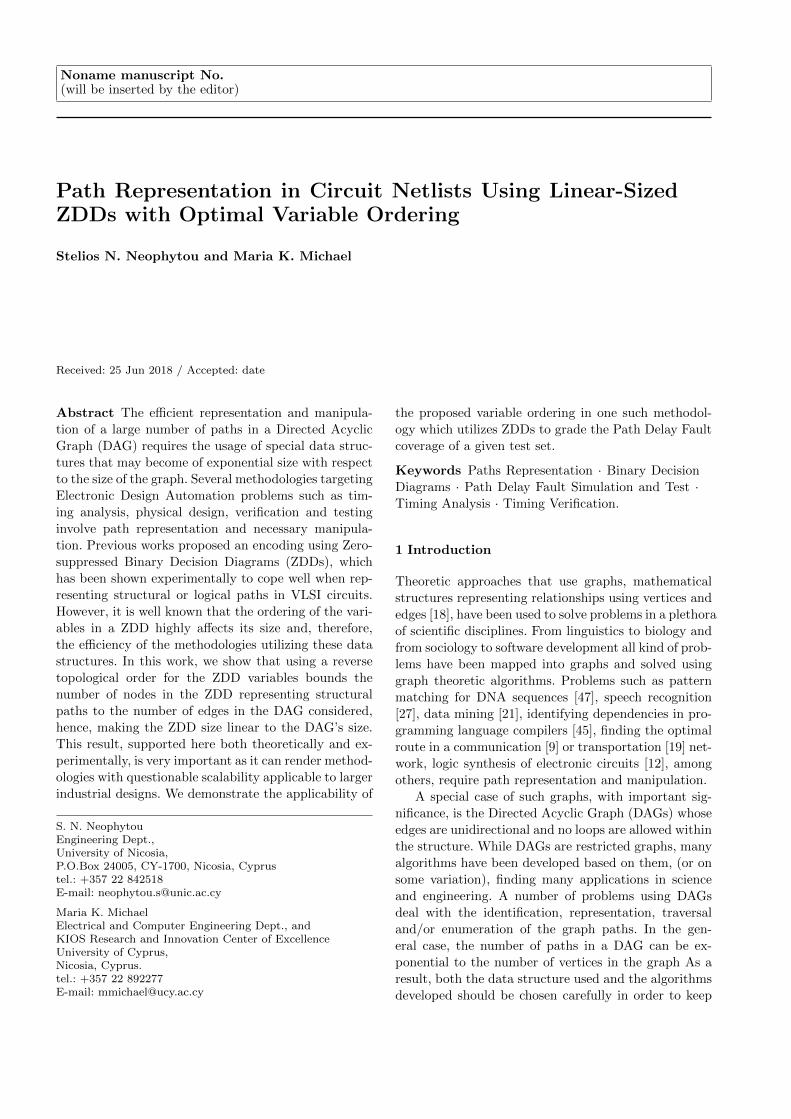
Fig. 1 Circuit C17 from ISCAS’85 benchmark suite: (a)netlist representation and (b) the corresponding DAG (wherea vertex vi corresponds to netlist line i).
In [36] a circuit structural path is encoded in a ZDD
as a binary combination. A structural path is a com-
plete I/O path, comprised of consecutive circuit inter-
connection lines. The encoding considers one ZDD vari-
able per circuit line. For each variable, one or more
nodes may exist at the same level in the ZDD. Each
node has two children (corresponding to the two possi-
ble decisions) reached by a 0-edge or a 1-edge. Follow-
ing a path in the ZDD an outgoing 1-edge from a node
means that the variable corresponding to the node ex-
ists (=1) in the combination. A 0-edge means that the
corresponding variable does not exist (=0) in the com-
bination. A path in the ZDD ending at the 1-terminal
node represents a variable combination (also known as
ZDD minterm).
As an example, consider the circuit in Fig. 1(a) with
its corresponding DAG in Fig. 1(b) and possible corre-
sponding ZDDs in Fig. 2. A vertex vi in the DAG in
Fig. 1(b) corresponds to the circuit line i in Fig. 1. Fig. 2
shows two possible ZDDs for the DAG in Fig. 1(b), each
using a different variable ordering. Both ZDDs have ex-
actly 17 levels (one per DAG vertex). The ordering of
the variables is shown on the left of each ZDD. A reverse
topological order is used in Fig. 2(a) and a BFS-based
order is used in Fig. 2(b). Dashed lines correspond to 0-
edges and solid lines to 1-edges. The square nodes cor-
respond to the root (top), 1-terminal, and 0-terminal
nodes. A path starting at the root node and ending at
the 1-terminal is a representation of a structural path
in the circuit. For example, consider the shaded path of
Fig. 2(a) which corresponds to the path 4-9-10-12-14-
16 marked by dashed lines in Fig. 1(a). The outgoing
0-edges from the ZDD nodes for variables v17 and v7in the shaded path indicate that lines 17 and 7 are
off-path. The remaining off-path lines are implied as
a suppressed node in a ZDD implies that the corre-
sponding variable assumes the 0 value. Observe that,
for the same path in a ZDD with different variable or-
der (such as that in Fig. 2(b)) different variables may
be suppressed or explicitly represented with outgoing 0-
edges. In this particular example, variables v1, v2 and
v3 are explicitly set to 0. A more detailed discussion on
the impact of variable ordering in ZDDs is presented in
Subsection 2.2.
The algorithm used to built the ZDD for all paths is
presented in Section 3, and it utilizes standard ZDD op-
erations to performed basic combinational set theoretic
operations, such as Union, Intersection, etc. Table 1
lists the basic ZDD operations and functions used in
this work as well as other relevant operations that can
be used in applications of the proposed method. With
Zi we denote a ZDD and with r a ZDD variable.
For example, if ZDD Union is applied between two
ZDDs Z1 and Z2, each representing a set of paths, a
new set of paths is created which includes all the paths
in either Z1, Z2, without any path duplication. Union
is performed in a non-enumerative manner with respect
to the paths. The same holds for many other set oper-
ations (including all listed in Table 1). This property
makes ZDDs very attractive as several operations can
be efficiently performed in time linear to the ZDD size.
The work of [25] proposed a more compact path
representation compared to the one in [36]. Specifically,
[25] shows that all paths can be represented using one
ZDD variable per primary input and one ZDD variable
per circuit branch line (referred to as primary lines).
This approach is suitable for the PDF test grading
problem and it constructs ZDDs with smaller size that
those in [36]. However, since the entire paths are not
kept in the structure, its applicability to other prob-
lems such that of [33] is not guaranteed. In Section 4
we consider both mappings (i.e, [36] and [25]) for rep-
Table 1 The basic ZDD operations.
ZDD Operation Description
searches for a set that consists of all combinationsZDD Getnode(r,Z1,Z2) in Z1 not containing variable r and all combinations
in Z2 containing variable r; creates the set if not exist
ZDD Change(Z,r) augments combinations of Z with element r
ZDD Union(Z1,Z2) returns the union of all combinations in Z1 and Z2
ZDD Difference(Z1,Z2) removes all combinations of Z2 from Z1
ZDD Intersect(Z1,Z2) returns the intersection of all combinations in Z1 and Z2
ZDD Count(Z) returns the number of combinations in Z
4 Stelios N. Neophytou and Maria K. Michael
(a) (b)
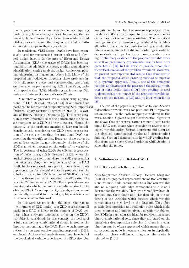
Fig. 2 The representation of the paths of C17 considering: (a) reverse topological order (b) BFS-based order.
resenting all structural paths and for PDF grading. In
order to underline the generality of the proposed ap-
proach the remaining of this paper considers standard
DAGs and, therefore, the complete path encoding of
[36] is used.
2.2 The Variable Ordering Challenge
A known problem that limits the usage of Reduced Or-
dered Binary Decision Diagrams (BDDs) is their sensi-
tivity on the variable ordering which can highly affect
their size. ZDDs are not an exception to this. Fig. 2 il-
lustrates the representation of all paths in the DAG of
Fig. 1(b), using two different variable orders. Fig. 2(a)
uses a variable ordering following a reverse topologi-
cal order of the DAG’s vertices while Fig. 2(b) uses a
Breadth First Search (BFS) order of the vertices (note
that the labels of the vertices of the DAG follow a topo-
logical order). Although the two diagrams hold exactly
the same paths, the representation in Fig. 2(a) is ob-
viously more compact and, thus, more efficient. The
reason for the increase of the ZDD size in Fig. 2(b)
is attributed to the duplication of nodes for some vari-
ables, created in order to preserve the correctness of the
representation. For example, there are three nodes for
variables v12 and v16 and two nodes per variable v7 and
v10. Nevertheless, note that there is a one-to-one cor-
respondence between the ZDDs’ paths and the DAG’s
paths. The shaded paths in Fig. 2(a) and Fig. 2(b) both
represent the dashed path in the DAG in Fig. 1(b).
To ensure an efficient variable ordering for the con-
struction of BDDs (and their variants), previous work
has followed two different directions. Static approaches
order the variable set prior to the construction of the
BDD whereas dynamic approaches allow for ordering
changes (re-ordering) during the construction of the
BDD when specific conditions are met (e.g. size increase
above a threshold).
Static ordering is in the general case less time and
resource consuming and has been preferred for this in
a number of previous works, [4,16] among many oth-
ers. Due to their small computational effort static tech-
niques are widely used and thoroughly explored. The
work of [10] summarizes and compares some of the most
effective static approaches.
On the other hand, dynamic approaches (also known
as dynamic reordering) may lead to more efficient rep-
resentations, where their application is not computa-
tionally prohibitive as their complexity is known to be
NP-complete [5]. The numerous heuristics that follow
the dynamic approach have been shown to work well
for specific problems although they still remain resource
demanding for large input instances [11,35,37,39]. An-
other reordering approach, mainly motivated by prob-
lems encountered in logic synthesis, tries to optimize the
BDD size after its construction (see [13,15,20] among
others). While many reordering approaches have been
Path Representation in Circuit Netlists Using Linear-Sized ZDDs with Optimal Variable Ordering 5
previously proposed with considerable reduction in the
size of the obtained BDD, they cannot control the size
of the BDD during construction and may result in irre-
versible size increase. The comprehensive work of [14]
summarizes these ordering approaches providing appro-
priate comparisons.
The BDD ordering techniques have been used in
the vast majority of the works for ZDDs. The works
in [21] and [24] attempt to incorporate concepts from
BDD variable ordering to ZDDs, both specific to the
problem they examine. None of these two methods pro-
vide an upper bound of the size of the obtained ZDD.
Specifically, [21] proposes a good variable order for fre-
quent itemsets used in data mining with very good im-
provements over the previously used approaches, yet its
applicability is limited to the problem considered. The
approach of [24] is also specific to the examined prob-
lem of path delay fault coverage calculation for digital
circuits. As this work also uses the PDF coverage prob-
lem to demonstrate the effectiveness of the proposed
theory, we have included appropriate discussion and ex-
perimentation in Section 4.
3 Path Representation using Linear Sized
ZDDs
This section firstly describes the basic steps of the ZDD-
based representation of the paths of a given DAG (Sub-
section 3.1). Then it presents reasoning proving that,
when using the proposed variable order, the ZDD size
is linear to the size of the initial DAG (Subsection 3.2).
The proposed ordering for the variables of the ZDD to
be constructed is taken based on the reverse topological
order of the DAG’s vertices. For the reverse topological
order each vertex in the DAG has higher order than any
of its predecessor vertices. The standard (not reverse)
topological order can be used with the same final mem-
ory requirements (but not the same peak memory re-
quirements). We propose the reverse topological order
for two reasons: (a) the ZDD is constructed faster, and
(b) the number of intermediate nodes is constant and
smaller than the standard topological order.
3.1 All-path ZDD Construction
The proposed algorithm performs a topological traver-
sal of the DAG and creates a ZDD per DAG vertex. The
ZDD at a vertex represents all the path segments up to
the vertex, starting from all vertices with no incoming
edges (0 in-degree). The final ZDD is then obtained by
unifying all ZDDs of the ending vertices (0 out-degree)
into a single ZDD.
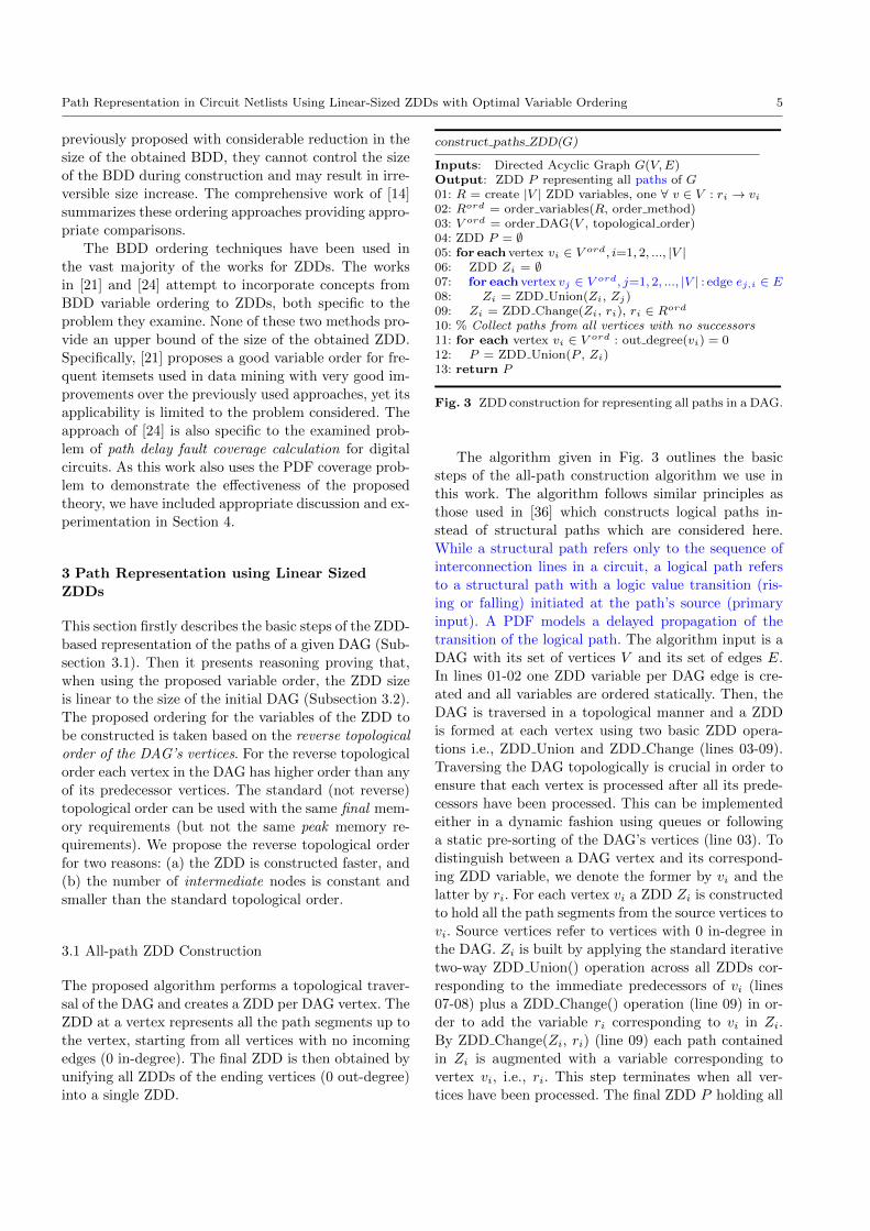
construct paths ZDD(G)
Inputs: Directed Acyclic Graph G(V,E)Output: ZDD P representing all paths of G01: R = create |V | ZDD variables, one ∀ v ∈ V : ri → vi02: Rord = order variables(R, order method)03: V ord = order DAG(V , topological order)04: ZDD P = ∅05: for each vertex vi ∈ V ord, i=1, 2, ..., |V |06: ZDD Zi = ∅07: for each vertex vj ∈ V ord, j=1, 2, ..., |V | : edge ej,i ∈ E08: Zi = ZDD Union(Zi, Zj)09: Zi = ZDD Change(Zi, ri), ri ∈ Rord
10: % Collect paths from all vertices with no successors11: for each vertex vi ∈ V ord : out degree(vi) = 012: P = ZDD Union(P , Zi)13: return P
Fig. 3 ZDD construction for representing all paths in a DAG.
The algorithm given in Fig. 3 outlines the basic
steps of the all-path construction algorithm we use in
this work. The algorithm follows similar principles as
those used in [36] which constructs logical paths in-
stead of structural paths which are considered here.
While a structural path refers only to the sequence of
interconnection lines in a circuit, a logical path refers
to a structural path with a logic value transition (ris-
ing or falling) initiated at the path’s source (primary
input). A PDF models a delayed propagation of the
transition of the logical path. The algorithm input is a
DAG with its set of vertices V and its set of edges E.
In lines 01-02 one ZDD variable per DAG edge is cre-
ated and all variables are ordered statically. Then, the
DAG is traversed in a topological manner and a ZDD
is formed at each vertex using two basic ZDD opera-
tions i.e., ZDD Union and ZDD Change (lines 03-09).
Traversing the DAG topologically is crucial in order to
ensure that each vertex is processed after all its prede-
cessors have been processed. This can be implemented
either in a dynamic fashion using queues or following
a static pre-sorting of the DAG’s vertices (line 03). To
distinguish between a DAG vertex and its correspond-
ing ZDD variable, we denote the former by vi and the
latter by ri. For each vertex vi a ZDD Zi is constructed
to hold all the path segments from the source vertices to
vi. Source vertices refer to vertices with 0 in-degree in
the DAG. Zi is built by applying the standard iterative
two-way ZDD Union() operation across all ZDDs cor-
responding to the immediate predecessors of vi (lines
07-08) plus a ZDD Change() operation (line 09) in or-
der to add the variable ri corresponding to vi in Zi.
By ZDD Change(Zi, ri) (line 09) each path contained
in Zi is augmented with a variable corresponding to
vertex vi, i.e., ri. This step terminates when all ver-
tices have been processed. The final ZDD P holding all
6 Stelios N. Neophytou and Maria K. Michael
paths in the DAG is constructed by taking the union of
all Zi corresponding to sink vertices (lines 11-12), i.e.,
vertices with 0 out-degree.
When the underlying DAG represents a combina-
tional circuit netlist, the size of the all-paths ZDD can
be optimized by reducing the number of ZDD variables;
vertices corresponding to branch lines in the circuit
can be excluded from the encoding without any impact
on the correctness of the representation. Furthermore,
when using ZDDs for the PDF fault grading problem,
the algorithm in Fig. 3 can be easily modified to con-
sider the mapping of [25] which uses ZDD variables
only for primary input and branch lines. Our analy-
sis in the next subsection on the number of necessary
ZDD nodes is given based on the generated encoding of
the paths using distinct ZDD variables for each vertex
in the DAG, and it holds for both the aforementioned
variable optimization encodings.
3.2 Optimality of the Proposed Variable Ordering for
Linear-sized All-Path ZDDs.
In the rest of this section we show that the algorithm in
Fig. 3 produces a ZDD of linear size with respect to the
size of the DAG whose paths are to be represented. To
show this, we provide analytical evidence that the ba-
sic ZDD operations used in the process of Fig. 3 do not
increase the ZDD size (in terms of nodes) beyond the
DAG size plus one, when its variable ordering follows a
reverse topological order on the DAG vertices. The op-
timality of the proposed ordering is then proven based
on the observation that each DAG vertex is processed
only once.
Before discussing the proof, we present the outline
of the two basic ZDD operations considered here, in
Fig. 4 together with the ZDD Getnode() operation nec-
essary for the realization of the other two. At this point
it is necessary to clarify the difference between a ZDD
variable and a ZDD node. A node is a vertex with two
possible children (one reached via the 0-edge and one
via the 1-edge). A node corresponds to a ZDD variable
which represents a problem’s attribute, in our case a
DAG’s vertex. While there is a one-to-one relationship
between a ZDD variable and a DAG vertex, there is a
many-to-one relationship between a ZDD node and a
ZDD variable. In other words, there may be more than
one nodes corresponding to the same variable (siblings)
since each sibling’s children may be different. For the
operations in Fig. 4, P.top refers to the top node of
ZDD P ; P0 and P1 point to the subdiagrams with root
at the 0-edge and 1-edge children nodes of P , respec-
tively. Comparisons are done considering the variable
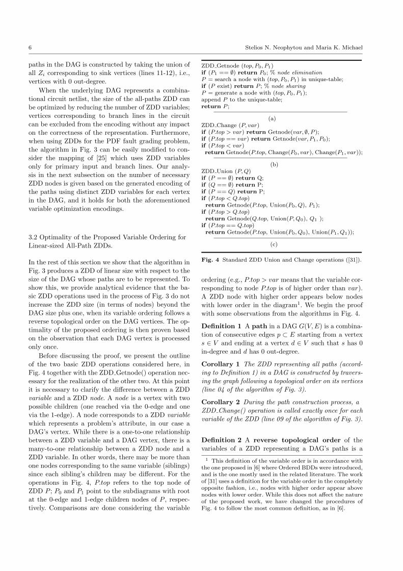
ZDD Getnode (top, P0, P1)if (P1 == ∅) return P0; % node eliminationP = search a node with (top, P0, P1) in unique-table;if (P exist) return P ; % node sharingP = generate a node with (top, P0, P1);append P to the unique-table;return P ;
(a)ZDD Change (P, var)if (P.top > var) return Getnode(var, ∅, P );if (P.top == var) return Getnode(var, P1, P0);if (P.top < var)return Getnode(P.top, Change(P0, var), Change(P1, var));
(b)ZDD Union (P,Q)if (P == ∅) return Q;if (Q == ∅) return P;if (P == Q) return P;if (P.top < Q.top)
return Getnode(P.top, Union(P0, Q), P1);if (P.top > Q.top)
return Getnode(Q.top, Union(P,Q0), Q1 );if (P.top == Q.top)
return Getnode(P.top, Union(P0, Q0), Union(P1, Q1));
(c)
Fig. 4 Standard ZDD Union and Change operations ([31]).
ordering (e.g., P.top > var means that the variable cor-
responding to node P.top is of higher order than var).
A ZDD node with higher order appears below nodes
with lower order in the diagram1. We begin the proof
with some observations from the algorithms in Fig. 4.
Definition 1 A path in a DAG G(V,E) is a combina-
tion of consecutive edges p ⊂ E starting from a vertex
s ∈ V and ending at a vertex d ∈ V such that s has 0
in-degree and d has 0 out-degree.
Corollary 1 The ZDD representing all paths (accord-
ing to Definition 1) in a DAG is constructed by travers-
ing the graph following a topological order on its vertices
(line 04 of the algorithm of Fig. 3).
Corollary 2 During the path construction process, a
ZDD Change() operation is called exactly once for each
variable of the ZDD (line 09 of the algorithm of Fig. 3).
Definition 2 A reverse topological order of the
variables of a ZDD representing a DAG’s paths is a
1 This definition of the variable order is in accordance withthe one proposed in [6] where Ordered BDDs were introduced,and is the one mostly used in the related literature. The workof [31] uses a definition for the variable order in the completelyopposite fashion, i.e., nodes with higher order appear abovenodes with lower order. While this does not affect the natureof the proposed work, we have changed the procedures ofFig. 4 to follow the most common definition, as in [6].
Path Representation in Circuit Netlists Using Linear-Sized ZDDs with Optimal Variable Ordering 7
numbering of the ZDD variables obtained by following
a topological visiting of the DAG’s vertices where each
variable is numbered in a decreasing order as the ver-
tices are visited.
Considering the DAG in Fig. 1(b), a topological visit
traverses the DAG in the (possible) order v1, v2, v3, v4,
v5, v6, v7, v8, v9, v10, v11, v12, v13, v14, v15, v16, v17 and the
corresponding reverse topological order of the variables
is defined as r17, r16, r15, r14, r13, r12, r11, r10, r9, r8, r7,
r6, r5, r4, r3, r2, r1 following the convention used in the
algorithm in Fig. 3.
The ZDD Getnode() operation (described in Fig. 4(a))
accepts as inputs a variable top and two sub-graphs
P0 and P1. It returns a node P corresponding to top
and with P0 and P1 connected to its 0-edge and 1-edge,
respectively. All nodes are kept to a structure called
unique table where no node (corresponding to the same
variable with the same children) exists twice. Analyzing
the ZDD Getnode() operation we identify two possibili-
ties: (i) such a ZDD node exists, no new node is created
and P is identical to that node, and (ii) such ZDD node
does not exist and P is created and added to the unique
table.
Corollary 3 A single call of ZDD Getnode(top, P0, P1)
function can create at most one new node for variable
top. A new node is constructed if and only if there ex-
ists no node in the unique table corresponding to top
having its 0-edge and 1-edge pointing to P0 and P1, re-
spectively.
Lemma 1 The ZDD Change(Zi, ri) operation at line
09 of process in Fig. 3 adds exactly one new node to
ZDD Zi which corresponds to variable ri when the ZDD
variables are ordered in a reverse topological order.
Proof Let Zi = P and ri = var based on the descrip-
tion of Fig. 4(b). ZDD Change(P, var) augments all
paths of ZDD P with variable var. This implies that, if
necessary, more than one nodes may be created to en-
sure the ZDD’s canonical attribute. However, a call of
ZDD Change() occurs only once (Corollary 2) and only
when all DAG vertices with lower topological order have
been visited (Corollary 1). From Definition 2, all vari-
ables in P have higher topological order than var. This
case falls under the first condition of the ZDD Change()
operation that calls a ZDD Getnode() operation once to
create or return a node corresponding to var. No such
node exists in the unique table because ZDD Getnode()
is called for the first time for var and, thus, from Corol-
lary 3, it follows that exactly one node is created. From
the latter and since a single ZDD Getnode() is called
for each ZDD Change() which in turn is called once
per ZDD variable, the lemma follows.
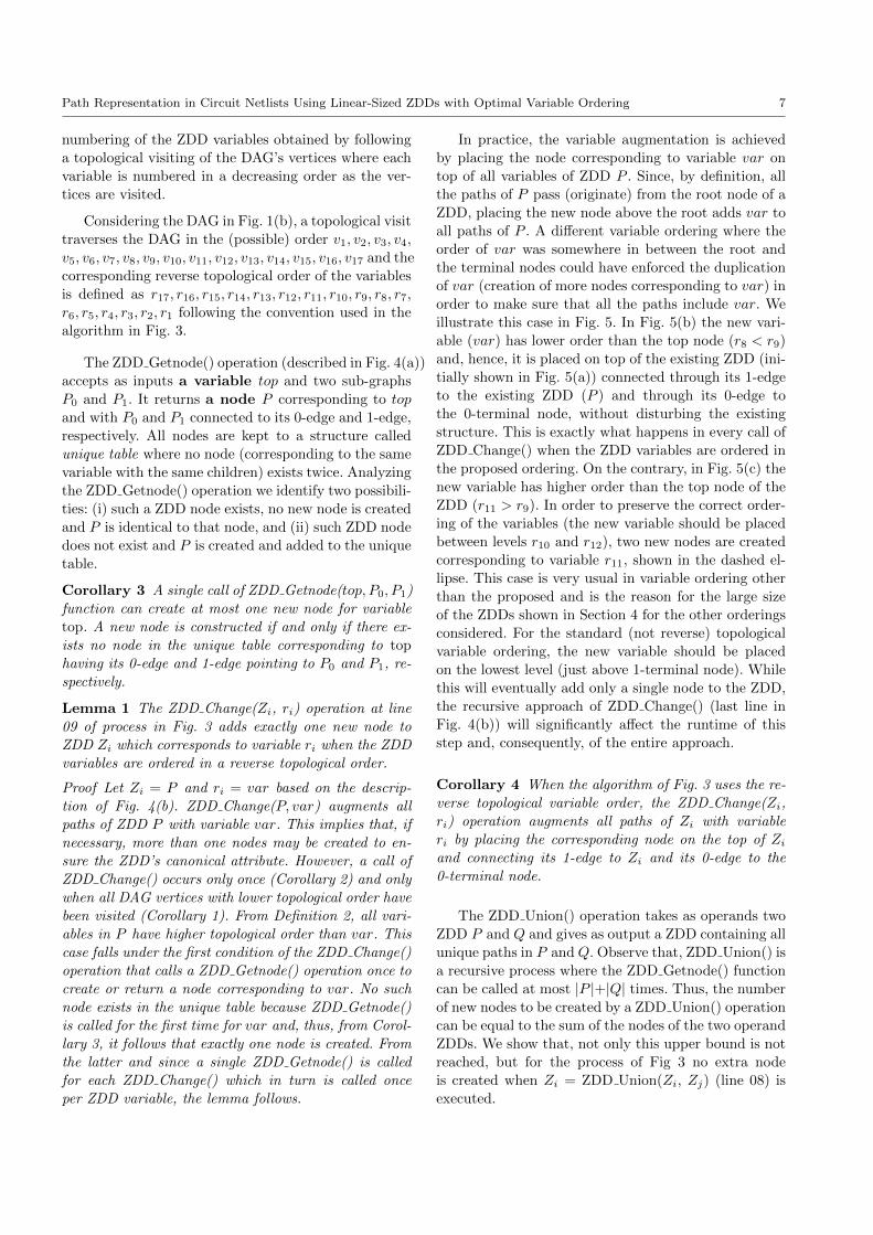
In practice, the variable augmentation is achieved
by placing the node corresponding to variable var on
top of all variables of ZDD P . Since, by definition, all
the paths of P pass (originate) from the root node of a
ZDD, placing the new node above the root adds var to
all paths of P . A different variable ordering where the
order of var was somewhere in between the root and
the terminal nodes could have enforced the duplication
of var (creation of more nodes corresponding to var) in
order to make sure that all the paths include var. We
illustrate this case in Fig. 5. In Fig. 5(b) the new vari-
able (var) has lower order than the top node (r8 < r9)
and, hence, it is placed on top of the existing ZDD (ini-
tially shown in Fig. 5(a)) connected through its 1-edge
to the existing ZDD (P ) and through its 0-edge to
the 0-terminal node, without disturbing the existing
structure. This is exactly what happens in every call of
ZDD Change() when the ZDD variables are ordered in
the proposed ordering. On the contrary, in Fig. 5(c) the
new variable has higher order than the top node of the
ZDD (r11 > r9). In order to preserve the correct order-
ing of the variables (the new variable should be placed
between levels r10 and r12), two new nodes are created
corresponding to variable r11, shown in the dashed el-
lipse. This case is very usual in variable ordering other
than the proposed and is the reason for the large size
of the ZDDs shown in Section 4 for the other orderings
considered. For the standard (not reverse) topological
variable ordering, the new variable should be placed
on the lowest level (just above 1-terminal node). While
this will eventually add only a single node to the ZDD,
the recursive approach of ZDD Change() (last line in
Fig. 4(b)) will significantly affect the runtime of this
step and, consequently, of the entire approach.
Corollary 4 When the algorithm of Fig. 3 uses the re-
verse topological variable order, the ZDD Change(Zi,
ri) operation augments all paths of Zi with variable
ri by placing the corresponding node on the top of Zi
and connecting its 1-edge to Zi and its 0-edge to the
0-terminal node.
The ZDD Union() operation takes as operands two
ZDD P and Q and gives as output a ZDD containing all
unique paths in P and Q. Observe that, ZDD Union() is
a recursive process where the ZDD Getnode() function
can be called at most |P |+|Q| times. Thus, the number
of new nodes to be created by a ZDD Union() operation
can be equal to the sum of the nodes of the two operand
ZDDs. We show that, not only this upper bound is not
reached, but for the process of Fig 3 no extra node
is created when Zi = ZDD Union(Zi, Zj) (line 08) is
executed.
8 Stelios N. Neophytou and Maria K. Michael
Fig. 5 An example of the ZDD Change() step. Variables corresponding to each node is shown on the left of each diagram.(a) Diagram before the ZDD Change() application. (b) The new variable has lower order than the root of the ZDD. (c) Thenew variable has higher order than the root of the ZDD.
Lemma 2 The Zi = ZDD Union(Zi, Zj) operation in
line 08 of the process in Fig. 3 does not create any new
ZDD nodes when its variables are ordered in a reverse
topological order.
Proof Let Zi = P and Zj = Q based on the description
of Fig. 4(c). Without loss of generality, let the outcome
of the ZDD Union() be assigned to a ZDD other than
Zi, let that be F . Analyzing the process in Fig. 4(c) we
identify 6 different cases based on the relationship be-
tween P and Q each of which corresponds to a line in
the corresponding pseudocode. The lemma holds for the
first three cases, i.e., P or Q equal to zero and P = Q in
a straightforward manner as it returns existing ZDDs
(either P or Q) which ensures no new node is created.
The last case (P.top == Q.top) implies at least two
nodes corresponding to the same variable. Since from
Lemma 1 the ZDD Change() operation creates exactly
one node each time it is called and because it is called
only once for each DAG vertex (Corollary 2), we will
consider this case only if the remaining two cases can
create multiple nodes per variable. The two remaining
cases (P.top < Q.top and P.top > Q.top) are symmetri-
cal and, thus, without loss of generality we consider only
the first. Both P and Q have been created by a prior call
of the ZDD Change() operation and, hence, from Corol-
lary 4 P0 and Q0 point to the 0-terminal node. Thus,
the call of ZDD Getnode() returns F with root node
F.top corresponding to the same variable as P.top, P1
connected to its 1-edge and Q connected to its 0-edge.
The latter occurs because the inline ZDD Union() op-
eration returns Q since P0 = 0 (case P == 0). F has
exactly the same number of nodes as that in both P and
Q, with its new node F.top replacing P.top and corre-
sponding exactly to the same variable. According to the
path construction process (Fig. 3) a ZDD Union() op-
eration takes place at the incoming edges of a DAG’s
vertex. By definition, P.top can only correspond to the
incoming edges of one vertex (that corresponding to F ).
Hence, P.top will never be used again in the remaining
steps of the process and can be immediately deleted from
the unique table. Therefore, the size of the unique table
is not changed because of the ZDD Union() call, and
the lemma follows.
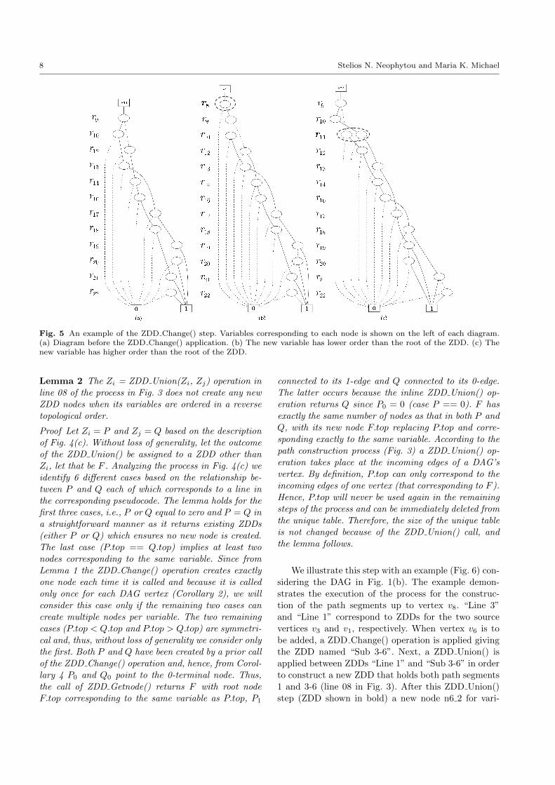
We illustrate this step with an example (Fig. 6) con-
sidering the DAG in Fig. 1(b). The example demon-
strates the execution of the process for the construc-
tion of the path segments up to vertex v8. “Line 3”
and “Line 1” correspond to ZDDs for the two source
vertices v3 and v1, respectively. When vertex v6 is to
be added, a ZDD Change() operation is applied giving
the ZDD named “Sub 3-6”. Next, a ZDD Union() is
applied between ZDDs “Line 1” and “Sub 3-6” in order
to construct a new ZDD that holds both path segments
1 and 3-6 (line 08 in Fig. 3). After this ZDD Union()
step (ZDD shown in bold) a new node n6 2 for vari-
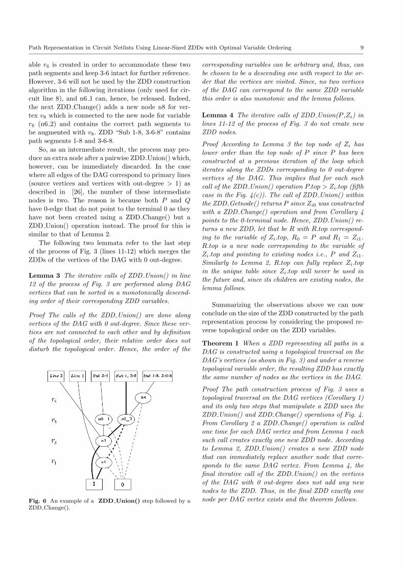
Path Representation in Circuit Netlists Using Linear-Sized ZDDs with Optimal Variable Ordering 9
able r6 is created in order to accommodate these two
path segments and keep 3-6 intact for further reference.
However, 3-6 will not be used by the ZDD construction
algorithm in the following iterations (only used for cir-
cuit line 8), and n6 1 can, hence, be released. Indeed,
the next ZDD Change() adds a new node n8 for ver-
tex v8 which is connected to the new node for variable
r6 (n6 2) and contains the correct path segments to
be augmented with v8. ZDD “Sub 1-8, 3-6-8” contains
path segments 1-8 and 3-6-8.
So, as an intermediate result, the process may pro-
duce an extra node after a pairwise ZDD Union() which,
however, can be immediately discarded. In the case
where all edges of the DAG correspond to primary lines
(source vertices and vertices with out-degree > 1) as
described in [26], the number of these intermediate
nodes is two. The reason is because both P and Q
have 0-edge that do not point to the terminal 0 as they
have not been created using a ZDD Change() but a
ZDD Union() operation instead. The proof for this is
similar to that of Lemma 2.
The following two lemmata refer to the last step
of the process of Fig. 3 (lines 11-12) which merges the
ZDDs of the vertices of the DAG with 0 out-degree.
Lemma 3 The iterative calls of ZDD Union() in line
12 of the process of Fig. 3 are performed along DAG
vertices that can be sorted in a monotonically descend-
ing order of their corresponding ZDD variables.
Proof The calls of the ZDD Union() are done along
vertices of the DAG with 0 out-degree. Since these ver-
tices are not connected to each other and by definition
of the topological order, their relative order does not
disturb the topological order. Hence, the order of the
Fig. 6 An example of a ZDD Union() step followed by aZDD Change().
corresponding variables can be arbitrary and, thus, can
be chosen to be a descending one with respect to the or-
der that the vertices are visited. Since, no two vertices
of the DAG can correspond to the same ZDD variable
this order is also monotonic and the lemma follows.
Lemma 4 The iterative calls of ZDD Union(P ,Zi) in
lines 11-12 of the process of Fig. 3 do not create new
ZDD nodes.
Proof According to Lemma 3 the top node of Zi has
lower order than the top node of P since P has been
constructed at a previous iteration of the loop which
iterates along the ZDDs corresponding to 0 out-degree
vertices of the DAG. This implies that for each such
call of the ZDD Union() operation P.top > Zi.top (fifth
case in the Fig. 4(c)). The call of ZDD Union() within
the ZDD Getnode() returns P since Zi0 was constructed
with a ZDD Change() operation and from Corollary 4
points to the 0-terminal node. Hence, ZDD Union() re-
turns a new ZDD, let that be R with R.top correspond-
ing to the variable of Zi.top, R0 = P and R1 = Zi1.
R.top is a new node corresponding to the variable of
Zi.top and pointing to existing nodes i.e., P and Zi1.
Similarly to Lemma 2, R.top can fully replace Zi.top
in the unique table since Zi.top will never be used in
the future and, since its children are existing nodes, the
lemma follows.
Summarizing the observations above we can now
conclude on the size of the ZDD constructed by the path
representation process by considering the proposed re-
verse topological order on the ZDD variables.
Theorem 1 When a ZDD representing all paths in a
DAG is constructed using a topological traversal on the
DAG’s vertices (as shown in Fig. 3) and under a reverse
topological variable order, the resulting ZDD has exactly
the same number of nodes as the vertices in the DAG.
Proof The path construction process of Fig. 3 uses a
topological traversal on the DAG vertices (Corollary 1)
and its only two steps that manipulate a ZDD uses the
ZDD Union() and ZDD Change() operations of Fig. 4.
From Corollary 2 a ZDD Change() operation is called
one time for each DAG vertex and from Lemma 1 each
such call creates exactly one new ZDD node. According
to Lemma 2, ZDD Union() creates a new ZDD node
that can immediately replace another node that corre-
sponds to the same DAG vertex. From Lemma 4, the
final iterative call of the ZDD Union() on the vertices
of the DAG with 0 out-degree does not add any new
nodes to the ZDD. Thus, in the final ZDD exactly one
node per DAG vertex exists and the theorem follows.
10 Stelios N. Neophytou and Maria K. Michael
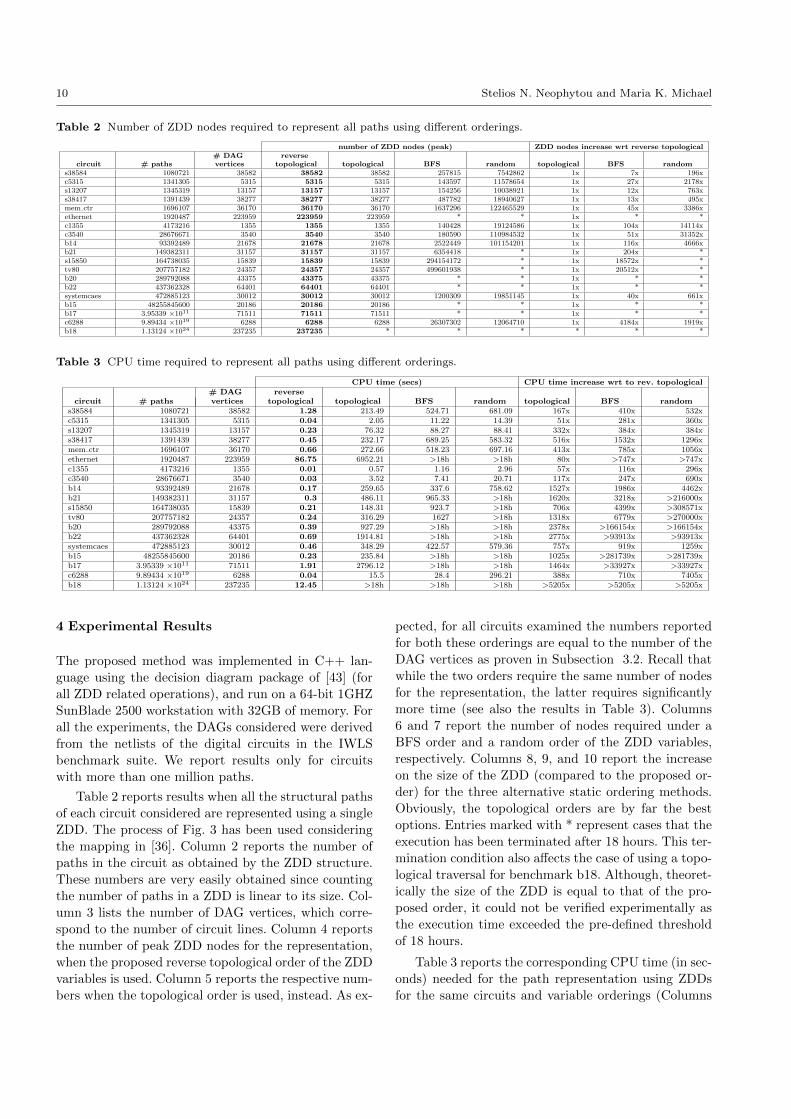
Table 2 Number of ZDD nodes required to represent all paths using different orderings.
number of ZDD nodes (peak) ZDD nodes increase wrt reverse topological# DAG reverse
circuit # paths vertices topological topological BFS random topological BFS randoms38584 1080721 38582 38582 38582 257815 7542862 1x 7x 196xc5315 1341305 5315 5315 5315 143597 11578654 1x 27x 2178xs13207 1345319 13157 13157 13157 154256 10038921 1x 12x 763xs38417 1391439 38277 38277 38277 487782 18940627 1x 13x 495xmem ctr 1696107 36170 36170 36170 1637296 122465529 1x 45x 3386xethernet 1920487 223959 223959 223959 * * 1x * *c1355 4173216 1355 1355 1355 140428 19124586 1x 104x 14114xc3540 28676671 3540 3540 3540 180590 110984532 1x 51x 31352xb14 93392489 21678 21678 21678 2522449 101154201 1x 116x 4666xb21 149382311 31157 31157 31157 6354418 * 1x 204x *s15850 164738035 15839 15839 15839 294154172 * 1x 18572x *tv80 207757182 24357 24357 24357 499601938 * 1x 20512x *b20 289792088 43375 43375 43375 * * 1x * *b22 437362328 64401 64401 64401 * * 1x * *systemcaes 472885123 30012 30012 30012 1200309 19851145 1x 40x 661xb15 48255845600 20186 20186 20186 * * 1x * *b17 3.95339 ×10¹¹ 71511 71511 71511 * * 1x * *c6288 9.89434 ×10¹⁹ 6288 6288 6288 26307302 12064710 1x 4184x 1919xb18 1.13124 ×1024 237235 237235 * * * * * *
Table 3 CPU time required to represent all paths using different orderings.
CPU time (secs) CPU time increase wrt to rev. topological# DAG reverse
circuit # paths vertices topological topological BFS random topological BFS randoms38584 1080721 38582 1.28 213.49 524.71 681.09 167x 410x 532xc5315 1341305 5315 0.04 2.05 11.22 14.39 51x 281x 360xs13207 1345319 13157 0.23 76.32 88.27 88.41 332x 384x 384xs38417 1391439 38277 0.45 232.17 689.25 583.32 516x 1532x 1296xmem ctr 1696107 36170 0.66 272.66 518.23 697.16 413x 785x 1056xethernet 1920487 223959 86.75 6952.21 >18h >18h 80x >747x >747xc1355 4173216 1355 0.01 0.57 1.16 2.96 57x 116x 296xc3540 28676671 3540 0.03 3.52 7.41 20.71 117x 247x 690xb14 93392489 21678 0.17 259.65 337.6 758.62 1527x 1986x 4462xb21 149382311 31157 0.3 486.11 965.33 >18h 1620x 3218x >216000xs15850 164738035 15839 0.21 148.31 923.7 >18h 706x 4399x >308571xtv80 207757182 24357 0.24 316.29 1627 >18h 1318x 6779x >270000xb20 289792088 43375 0.39 927.29 >18h >18h 2378x >166154x >166154xb22 437362328 64401 0.69 1914.81 >18h >18h 2775x >93913x >93913xsystemcaes 472885123 30012 0.46 348.29 422.57 579.36 757x 919x 1259xb15 48255845600 20186 0.23 235.84 >18h >18h 1025x >281739x >281739xb17 3.95339 ×10¹¹ 71511 1.91 2796.12 >18h >18h 1464x >33927x >33927xc6288 9.89434 ×10¹⁹ 6288 0.04 15.5 28.4 296.21 388x 710x 7405xb18 1.13124 ×1024 237235 12.45 >18h >18h >18h >5205x >5205x >5205x
4 Experimental Results
The proposed method was implemented in C++ lan-
guage using the decision diagram package of [43] (for
all ZDD related operations), and run on a 64-bit 1GHZ
SunBlade 2500 workstation with 32GB of memory. For
all the experiments, the DAGs considered were derived
from the netlists of the digital circuits in the IWLS
benchmark suite. We report results only for circuits
with more than one million paths.
Table 2 reports results when all the structural paths
of each circuit considered are represented using a single
ZDD. The process of Fig. 3 has been used considering
the mapping in [36]. Column 2 reports the number of
paths in the circuit as obtained by the ZDD structure.
These numbers are very easily obtained since counting
the number of paths in a ZDD is linear to its size. Col-
umn 3 lists the number of DAG vertices, which corre-
spond to the number of circuit lines. Column 4 reports
the number of peak ZDD nodes for the representation,
when the proposed reverse topological order of the ZDD
variables is used. Column 5 reports the respective num-
bers when the topological order is used, instead. As ex-
pected, for all circuits examined the numbers reported
for both these orderings are equal to the number of the
DAG vertices as proven in Subsection 3.2. Recall thatwhile the two orders require the same number of nodes
for the representation, the latter requires significantly
more time (see also the results in Table 3). Columns
6 and 7 report the number of nodes required under a
BFS order and a random order of the ZDD variables,
respectively. Columns 8, 9, and 10 report the increase
on the size of the ZDD (compared to the proposed or-
der) for the three alternative static ordering methods.
Obviously, the topological orders are by far the best
options. Entries marked with * represent cases that the
execution has been terminated after 18 hours. This ter-
mination condition also affects the case of using a topo-
logical traversal for benchmark b18. Although, theoret-
ically the size of the ZDD is equal to that of the pro-
posed order, it could not be verified experimentally as
the execution time exceeded the pre-defined threshold
of 18 hours.
Table 3 reports the corresponding CPU time (in sec-
onds) needed for the path representation using ZDDs
for the same circuits and variable orderings (Columns
Path Representation in Circuit Netlists Using Linear-Sized ZDDs with Optimal Variable Ordering 11
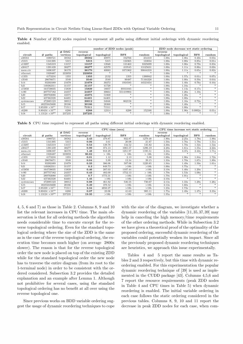
Table 4 Number of ZDD nodes required to represent all paths using different initial orderings with dynamic reorderingenabled.
number of ZDD nodes (peak) ZDD node decrease wrt static ordering# DAG reverse reverse
circuit # paths vertices topological topological BFS random topological topological BFS randoms38584 1080721 38582 38582 40975 102766 254318 1.00x 1.06x 0.40x 0.03xc5315 1341305 5315 5315 5315 122365 133034 1.00x 1.00x 0.85x 0.01xs13207 1345319 13157 13157 13948 121463 8325699 1.00x 1.06x 0.79x 0.83xs38417 1391439 38277 38277 42570 419545 13125631 1.00x 1.11x 0.86x 0.69xmem ctr 1696107 36170 36170 40083 1071962 99844318 1.00x 1.11x 0.65x 0.82xethernet 1920487 223959 223959 * * * 1.00x * * *c1355 4173216 1355 1355 2132 1355 1390942 1.00x 1.57x 0.01x 0.07xc3540 28676671 3540 3540 3540 90487 71164328 1.00x 1.00x 0.50x 0.64xb14 93392489 21678 21678 30272 1924585 44521654 1.00x 1.40x 0.76x 0.44xb21 149382311 31157 31157 41720 * * 1.00x 1.34x * *s15850 164738035 15839 15839 18057 49161045 * 1.00x 1.14x 0.17x *tv80 207757182 24357 24357 30664 551419904 * 1.00x 1.26x 1.10x *b20 289792088 43375 43375 51869 * * 1.00x 1.20x * *b22 437362328 64401 64401 64401 * * 1.00x 1.00x * *systemcaes 472885123 30012 30012 34846 862158 * 1.00x 1.16x 0.72x *b15 48255845600 20186 20186 28360 * * 1.00x 1.40x * *b17 3.95339 ×10¹¹ 71511 71511 71511 * * 1.00x 1.00x * *c6288 9.89434 ×10¹⁹ 6288 6288 12314 6288 152166 1.00x 1.96x 0.0002x 0.01xb18 1.13124 ×1024 237235 237235 * * * 1.00x * * *
Table 5 CPU time required to represent all paths using different initial orderings with dynamic reordering enabled.
CPU time (secs) CPU time increase wrt static ordering# DAG reverse reverse
circuit # paths vertices topological topological BFS random topological topological BFS randoms38584 1080721 38582 2.43 479.87 932.87 1279.48 1.90x 2.25x 1.78x 1.88xc5315 1341305 5315 0.06 3.61 20.08 21.67 1.50x 1.76x 1.79x 1.51xs13207 1345319 13157 0.53 129.78 134.52 135.82 2.30x 1.70x 1.52x 1.54xs38417 1391439 38277 0.99 374.13 1065.57 1296.19 2.20x 1.61x 1.55x 2.22xmem ctr 1696107 36170 1.48 918.29 1251.97 1195.51 2.24x 3.37x 2.42x 1.71xethernet 1920487 223959 90.82 > 18h > 18h > 18h 1.05x * * *c1355 4173216 1355 0.01 1.12 2.13 5.08 1.00x 1.96x 1.84x 1.72xc3540 28676671 3540 0.04 5.99 12.34 39.15 1.33x 1.70x 1.67x 1.89xb14 93392489 21678 0.33 386.06 507.06 1220.85 1.94x 1.49x 1.50x 1.61xb21 149382311 31157 0.3 849.73 >18h >18h 1.00x 1.75x * *s15850 164738035 15839 0.46 207.03 1107.44 >18h 2.19x 1.40x 1.20x *tv80 207757182 24357 0.43 483.09 1752.13 > 18h 1.79x 1.53x 1.08x *b20 289792088 43375 0.7 1773.31 >18h >18h 1.79x 1.91x * *b22 437362328 64401 1.45 >18h >18h >18h 2.10x * * *systemcaes 472885123 30012 0.98 461.82 546.55 730.67 2.13x 1.33x 1.29x 1.26xb15 48255845600 20186 0.49 378.52 >18h >18h 2.13x 1.60x * *b17 3.95339 ×10¹¹ 71511 2.34 4850.27 >18h >18h 1.23x 1.73x * *c6288 9.89434 ×10¹⁹ 6288 0.07 23.06 41.63 985.11 1.75x 1.49x 1.47x 3.33xb18 1.13124 ×1024 237235 19.35 >18h >18h >18h 1.55x * * *
4, 5, 6 and 7) as those in Table 2. Columns 8, 9 and 10list the relevant increases in CPU time. The main ob-
servation is that for all ordering methods the algorithm
needs considerable time to execute except for the re-
verse topological ordering. Even for the standard topo-
logical ordering where the size of the ZDD is the same
as in the case of the reverse topological ordering, the ex-
ecution time becomes much higher (on average 2800x
slower). The reason is that for the reverse topological
order the new node is placed on top of the existing ZDD
while for the standard topological order the new node
has to traverse the entire diagram (from its root to the
1-terminal node) in order to be consistent with the or-
dered considered. Subsection 3.2 provides the detailed
explanation and an example after Lemma 1. Although
not prohibitive for several cases, using the standard
topological ordering has no benefit at all over using the
reverse topological one.
Since previous works on BDD variable ordering sug-
gest the usage of dynamic reordering techniques to cope
with the size of the diagram, we investigate whether a
dynamic reordering of the variables [11,35,37,39] may
help in canceling the high memory/time requirements
of the other ordering methods. While in Subsection 3.2
we have given a theoretical proof of the optimality of the
proposed ordering, successful dynamic reordering of the
variables could potentially weaken its impact. Since all
the previously proposed dynamic reordering techniques
are heuristics, we approach this issue experimentally.
Tables 4 and 5 report the same results as Ta-
bles 2 and 3 respectively, but this time with dynamic re-
ordering enabled. For this experimentation the popular
dynamic reordering technique of [39] is used as imple-
mented in the CUDD package [43]. Columns 4,5,6 and
7 report the resource requirements (peak ZDD nodes
in Table 4 and CPU times in Table 5) when dynamic
reordering is enabled. The initial variable ordering in
each case follows the static ordering considered in the
previous tables. Columns 8, 9, 10 and 11 report the
decrease in peak ZDD nodes for each case, when com-
12 Stelios N. Neophytou and Maria K. Michael
pared to the required peak nodes of the static ordering
approaches (columns 4-7 of Table 2). For example, con-
sider circuit s38584. When dynamic reordering is en-
abled the node count for the BFS ordering is reduced
to 0.4x of the nodes required when a purely static order-
ing approach is used. This is calculated by comparing
the 257815 nodes required when BFS ordering is ap-
plied without dynamic reordering enabled (Column 6
of Table 2) with the 102766 nodes required when dy-
namic reordering was enabled (Column 6 of Table 4).
Of course this is done in the expense of CPU time which
is increased by 78% (Column 9 of Table 5) with respect
to the BFS ordering without the dynamic reordering.
Entries with * denote that the comparison is not possi-
ble as the execution takes excessive CPU time, meeting
the termination condition of 18 hours.
The obvious finding from this investigation is that
dynamic reordering increases the execution times con-
siderably. In all reported cases the execution time is
higher than the time required for the corresponding
static variable ordering approaches. For the BFS and
Random orderings the node counts are decreased, for
some cases significantly, with dynamic reordering. This
shows effective exploitation of the extra CPU time, al-
though in all cases the obtained node counts are much
higher that those obtained using the proposed opti-
mal static reverse topological order. For example, for
s38584, the node count using the random variable or-
dering is 33 times smaller when dynamic reordering is
enabled. Nevertheless, this gives a peak node count of
254318 which is 6.6 times larger than the node count
when the reverse topological order is used without dy-
namic reordering. Dynamic reordering manages to match
the optimal order only for circuits c1355 and c6288,
when an initial BFS order is used. Note that dynamic
reordering increases the CPU time even in the case
of the optimal ordering which is attributed to the ex-
tra condition checks performed by dynamic reordering
(even when no reordering is actually performed). Fi-
nally, dynamic reordering negatively affects the stan-
dard topological ordering for both metrics. While the
CPU time needed is increased as in all cases, the node
count does not decrease, on the contrary, in many cases
it increases considerably.
5 Application to Path Delay Fault Grading
Previous work on path representation in digital circuits
has been developed in relation to the Path Delay Fault
(PDF) model [42], where a fault is a logical circuit
path modeled as a delayed transition across a struc-
tural path. Several related problems have been inves-
tigated, for the PDF model including PDF simulation
(or grading) [2,17,24,28,36,41].
Path enumerative methods are inherently problem-
atic for this problem due to the large number of paths
in a circuit, while the early non-enumerative methods
give only a pessimistic estimation of the fault coverage
[2]. The first work that proposed an exact methodology
for PDF fault coverage calculation used a special data
structure called path-status graph [17]. This data struc-
ture can become of exponential size with respect to the
size of the circuit considered. [36] also proposed an exact
algorithm using ZDDs. While the latter method can, in
the worst case, result in an exponentially large struc-
ture, in practice ZDDs have been shown to cope well
when representing paths. A preliminary experimental
study investigating the size of ZDDs when representing
paths under different ZDD variable orderings was per-
formed in [24]. Yet, none of the existing works addresses
the complexity and optimality of the variable ordering.
In this section we consider the PDF grading prob-
lem i.e., the exact calculation of the fault coverage of a
test set with respect to the PDF model, when ZDDs are
used under the proposed optimal variable ordering. For
every structural path 2 PDFs are modeled, one with
a rising and one with a falling transition in the path’s
input. A valid test for a PDF is a pair of input vectors
(t1, t2) that excites the associated transition at the first
node of the PDF (primary input or scan chain element)
and allows its propagation to an observable point (ei-
ther primary output or scan chain element). Tests may
consider different sensitization conditions for the cir-
cuit lines affecting the propagation, namely the lines
that are side inputs to the gates and are not on the
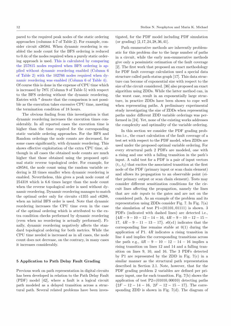
considered path. As an example of the problem and its
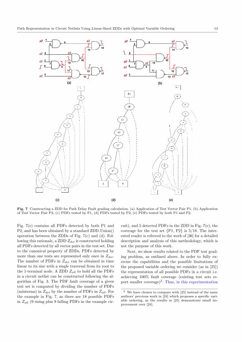
representation using ZDDs consider Fig. 7. In Fig. 7(a)
the simulation of test P1=(01101, 01111) is shown. 3
PDFs (indicated with dashed lines) are detected i.e.,
{4R − 9− 10− 12− 14− 16, 4R − 9− 10− 12− 15−17, 4R − 9 − 11 − 13 − 17}. s0(s1) indicates that the
corresponding line remains stable at 0(1) during the
application of P1. 4R indicates a rising transition in
line 4 and implies the corresponding transitions across
the path e.g., 4R − 9 − 10 − 12 − 14 − 16 implies a
rising transition on lines 12 and 14 and a falling tran-
sition on lines 9, 10, and 16. The 3 PDFs detected
by P1 are represented by the ZDD in Fig. 7(c) in a
similar manner as the structural path representation
described in Section 2.1. Note, however, that for the
PDF grading problem 2 variables are defined per pri-
mary input, one for each transition. Fig. 7(b) shows the
application of test P2=(01010, 00010) detecting paths
{2F − 12 − 14 − 16, 2F − 12 − 15 − 17}. The corre-
sponding ZDD is shown in Fig. 7(d). The diagram of
Path Representation in Circuit Netlists Using Linear-Sized ZDDs with Optimal Variable Ordering 13
s0
s1 s1
s1
(a)
(c) (d) (e)
15
(b)
s1
s1
s1
s1
s0
s0
s1 s0
s1
s1
Fig. 7 Constructing a ZDD for Path Delay Fault grading calculation. (a) Application of Test Vector Pair P1, (b) Applicationof Test Vector Pair P2, (c) PDFs tested by P1, (d) PDFs tested by P2, (e) PDFs tested by both P1 and P2.
Fig. 7(e) contains all PDFs detected by both P1 and
P2, and has been obtained by a standard ZDD Union()
operation between the ZDDs of Fig. 7(c) and (d). Fol-
lowing this rationale, a ZDD Zdet is constructed holding
all PDFs detected by all vector pairs in the test set. Due
to the canonical property of ZDDs, PDFs detected by
more than one tests are represented only once in Zdet.
The number of PDFs in Zdet can be obtained in time
linear to its size with a single traversal from its root to
the 1-terminal node. A ZDD Zall to hold all the PDFs
in a circuit netlist can be constructed following the al-
gorithm of Fig. 3. The PDF fault coverage of a given
test set is computed by dividing the number of PDFs
(minterms) in Zdet by the number of PDFs in Zall. For
the example in Fig. 7, as there are 18 possible PDFs
in Zall (9 rising plus 9 falling PDFs in the example cir-
cuit), and 5 detected PDFs in the ZDD in Fig. 7(e), the
coverage for the test set {P1, P2} is 5/18. The inter-
ested reader is referred to the work of [36] for a detailed
description and analysis of this methodology, which is
not the purpose of this work.
Next, we show results related to the PDF test grad-
ing problem, as outlined above. In order to fully ex-
ercise the capabilities and the possible limitations of
the proposed variable ordering we consider (as in [25])
the representation of all possible PDFs in a circuit i.e.
achieving 100% fault coverage (existing test sets re-
port smaller coverage)2. Thus, in this experimentation
2 We have chosen to compare with [25] instead of the sameauthors’ previous work in [24] which proposes a specific vari-able ordering, as the results in [25] demonstrate small im-provement over [24].
14 Stelios N. Neophytou and Maria K. Michael
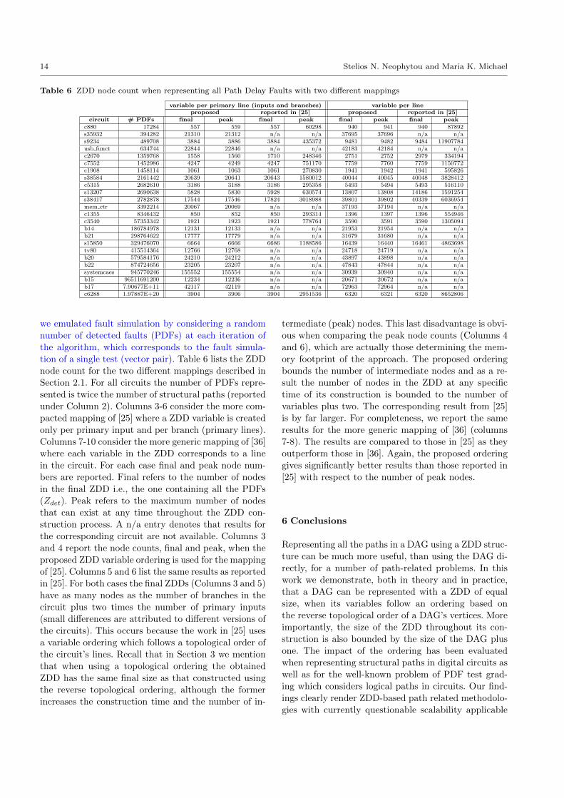
Table 6 ZDD node count when representing all Path Delay Faults with two different mappings
variable per primary line (inputs and branches) variable per lineproposed reported in [25] proposed reported in [25]
circuit # PDFs final peak final peak final peak final peakc880 17284 557 559 557 60298 940 941 940 87892s35932 394282 21310 21312 n/a n/a 37695 37696 n/a n/as9234 489708 3884 3886 3884 435372 9481 9482 9484 11907784usb funct 634744 22844 22846 n/a n/a 42183 42184 n/a n/ac2670 1359768 1558 1560 1710 248346 2751 2752 2979 334194c7552 1452986 4247 4249 4247 751170 7759 7760 7759 1150772c1908 1458114 1061 1063 1061 270830 1941 1942 1941 595826s38584 2161442 20639 20641 20643 1580012 40044 40045 40048 3828412c5315 2682610 3186 3188 3186 295358 5493 5494 5493 516110s13207 2690638 5828 5830 5928 630574 13807 13808 14186 1591254s38417 2782878 17544 17546 17824 3018988 39801 39802 40339 6036954mem ctr 3392214 20067 20069 n/a n/a 37193 37194 n/a n/ac1355 8346432 850 852 850 293314 1396 1397 1396 554946c3540 57353342 1921 1923 1921 778764 3590 3591 3590 1305094b14 186784978 12131 12133 n/a n/a 21953 21954 n/a n/ab21 298764622 17777 17779 n/a n/a 31679 31680 n/a n/as15850 329476070 6664 6666 6686 1188586 16439 16440 16461 4863698tv80 415514364 12766 12768 n/a n/a 24718 24719 n/a n/ab20 579584176 24210 24212 n/a n/a 43897 43898 n/a n/ab22 874724656 23205 23207 n/a n/a 47843 47844 n/a n/asystemcaes 945770246 155552 155554 n/a n/a 30939 30940 n/a n/ab15 96511691200 12234 12236 n/a n/a 20671 20672 n/a n/ab17 7.90677E+11 42117 42119 n/a n/a 72963 72964 n/a n/ac6288 1.97887E+20 3904 3906 3904 2951536 6320 6321 6320 8652806
we emulated fault simulation by considering a random
number of detected faults (PDFs) at each iteration of
the algorithm, which corresponds to the fault simula-
tion of a single test (vector pair). Table 6 lists the ZDD
node count for the two different mappings described in
Section 2.1. For all circuits the number of PDFs repre-
sented is twice the number of structural paths (reported
under Column 2). Columns 3-6 consider the more com-
pacted mapping of [25] where a ZDD variable is created
only per primary input and per branch (primary lines).
Columns 7-10 consider the more generic mapping of [36]
where each variable in the ZDD corresponds to a line
in the circuit. For each case final and peak node num-
bers are reported. Final refers to the number of nodes
in the final ZDD i.e., the one containing all the PDFs
(Zdet). Peak refers to the maximum number of nodes
that can exist at any time throughout the ZDD con-
struction process. A n/a entry denotes that results for
the corresponding circuit are not available. Columns 3
and 4 report the node counts, final and peak, when the
proposed ZDD variable ordering is used for the mapping
of [25]. Columns 5 and 6 list the same results as reported
in [25]. For both cases the final ZDDs (Columns 3 and 5)
have as many nodes as the number of branches in the
circuit plus two times the number of primary inputs
(small differences are attributed to different versions of
the circuits). This occurs because the work in [25] uses
a variable ordering which follows a topological order of
the circuit’s lines. Recall that in Section 3 we mention
that when using a topological ordering the obtained
ZDD has the same final size as that constructed using
the reverse topological ordering, although the former
increases the construction time and the number of in-
termediate (peak) nodes. This last disadvantage is obvi-
ous when comparing the peak node counts (Columns 4
and 6), which are actually those determining the mem-
ory footprint of the approach. The proposed ordering
bounds the number of intermediate nodes and as a re-
sult the number of nodes in the ZDD at any specific
time of its construction is bounded to the number of
variables plus two. The corresponding result from [25]
is by far larger. For completeness, we report the same
results for the more generic mapping of [36] (columns
7-8). The results are compared to those in [25] as they
outperform those in [36]. Again, the proposed ordering
gives significantly better results than those reported in
[25] with respect to the number of peak nodes.
6 Conclusions
Representing all the paths in a DAG using a ZDD struc-
ture can be much more useful, than using the DAG di-
rectly, for a number of path-related problems. In this
work we demonstrate, both in theory and in practice,
that a DAG can be represented with a ZDD of equal
size, when its variables follow an ordering based on
the reverse topological order of a DAG’s vertices. More
importantly, the size of the ZDD throughout its con-
struction is also bounded by the size of the DAG plus
one. The impact of the ordering has been evaluated
when representing structural paths in digital circuits as
well as for the well-known problem of PDF test grad-
ing which considers logical paths in circuits. Our find-
ings clearly render ZDD-based path related methodolo-
gies with currently questionable scalability applicable
Path Representation in Circuit Netlists Using Linear-Sized ZDDs with Optimal Variable Ordering 15
to large industrial designs, among a plethora of other
applications.
References
1. Ababei, C., Selvakkumaran, N., Bazargan, K., Karypis,G.: Multi-objective circuit partitioning for cutsize andpath-based delay minimization. In: Proc. of InternationalConference on CAD, pp. 181–185 (2002)
2. Abdulrazzaq, N.M., Gupta, S.K.: Path-delay fault simu-lation for circuits with large numbers of paths for verylarge test sets. In: Proc. of VLSI Test Symposium, pp.186–193 (2003)
3. Abramovici, M., Menon, P., Miller, D.T.: Critical pathtracing: An alternative to fault simulation. IEEE Design& Test of Computers 1(1), 83–93 (1984)
4. Aloul, F.A., Markov, I.L., Sakallah, K.A.: Mince: A staticglobal variable-ordering heuristic for SAT search andBDD manipulation. J. UCS 10(12), 1562–1596 (2004)
5. Bollig, B., Wegener, I.: Improving the variable orderingof OBDDs is NP-complete. IEEE Trans. on Computers,45(9), 993–1002 (1996)
6. Bryant, R.: Graph-Based Algorithms for Boolean Func-tion Manipulation. IEEE Trans. on Computers C-35(8),677–691 (1986)
7. Cheng, K.T., Chen, H.C.: Classification and identifica-tion of nonrobust untestable path delay faults. IEEETrans. on CAD of Integrated Circuits and Systems 15(8),845–853 (1996)
8. Christou, K., Michael, M.K., Tragoudas, S.: On the useof ZBDDs for implicit and compact critical PDF test gen-eration. J of Electronic Testing 24(1-3), 203–222 (2008)
9. Cruz, R., Santhanam, A.: Optimal routing, link schedul-ing and power control in multihop wireless networks. In:Proc. of IEEE INFOCOM, vol. 1, pp. 702–711 (2003)
10. Drechsler, R.: Evaluation of static variable orderingheuristics for MDD construction. In: Proc. of Inter. Sym-posium on Multiple-Valued Logic, pp. 254–260 (2002)
11. Drechsler, R., Gunther, W., Somenzi, F.: Using lowerbounds during dynamic BDD minimization. IEEE Trans.on CAD of Integrated Circuits and Systems, 20(1), 51–57(2001)
12. Drechsler, R., Shi, J., Fey, G.: Synthesis of fully testablecircuits from BDDs. IEEE Trans. on CAD of IntegratedCircuits and Systems 23(3), 440–443 (2004)
13. Ebendt, R., Drechsler, R.: Approximate BDD minimiza-tion by weighted A. In: Proc. of International Symposiumon Circuits and Systems, pp. 2974–2977 (2009)
14. Ebendt, R., Fey, G., Drechsler, R.: Advanced BDD opti-mization. Springer Science & Business Media (2005)
15. Friedman, S.J., Supowit, K.J.: Finding the optimal vari-able ordering for binary decision diagrams. In: Proc. ofInternational Conference on CAD, pp. 348–356 (1987)
16. Fujita, M., Fujisawa, H., Matsunaga, Y.: Variable order-ing algorithms for ordered binary decision diagrams andtheir evaluation. IEEE Trans on CAD of Integrated Cir-cuits and Systems 12(1), 6–12 (1993)
17. Gharaybeh, M.A., Bushnell, M.L., Agrawal, V.D.: Thepath-status graph with application to delay fault simu-lation. IEEE Trans. on CAD of Integrated Circuits andSystems 17(4), 324–332 (1998)
18. Gibbons, A.: Algorithmic Graph Theory. CambridgeUniv. Press (1985)
19. Goczy lla, K., Cielatkowski, J.: Optimal routing in atransportation network. European J. of Operational Re-search 87(2), 214–222 (1995)
20. Ishiura, N., Sawada, H., Yajima, S.: Minimazation of bi-nary decision diagrams based on exchanges of variables.In: Proc. of International Conference on CAD, vol. 91,pp. 472–475 (1991)
21. Iwasaki, H., Minato, S.i., Zeugmann, T.: A method ofvariable ordering for zero-suppressed binary decision di-agrams in data mining applications. In: Proc. of Interna-tional Workshop on Databases for Next Generation Re-searchers, pp. 85–90. IEEE (2007)
22. Iwashita, H., Kawahara, J., Minato, S.i.: ZDD-basedcomputation of the number of paths in a graph. HokkaidoUniversity, Division of Computer Science, TCS TechnicalReports, vol. TCS-TR-A-10-60 (2012)
23. Knuth, D.E.: The Art of Computer Programming, Vol-ume 4, Fascicles 0-4, 1st edn. Addison-Wesley Profes-sional (2009)
24. Kocan, F., Gunes, M., Thornton, M.A.: Static variableordering in ZBDDs for path delay fault coverage calcu-lation. In: Proc. of Midwest Symposium on Circuits andSystems, vol. 1, pp. 497–500 (2004)
25. Kocan, F., Gunes, M.H.: On the ZBDD-based nonenu-merative path delay fault coverage calculation. IEEETrans. on CAD of Integrated Circuits and Systems 24(7),1137–1143 (2005)
26. Kocan, F., Li, L., Saab, D.G.: Exact path delay faultcoverage calculation of partitioned circuits. IEEE Trans.on Computers 58(6), 858–864 (2009)
27. Kurai, R., Minato, S.i., Zeugmann, T.: N-gram analysisbased on zero-suppressed BDDs. In: Proc. of New Fron-tiers in Artificial Intelligence, pp. 289–300 (2007)
28. Lenox, J., Tragoudas, S.: Adapting an implicit path delaygrading method for parallel architectures. IEEE Trans.on CAD of Integrated Circuits and Systems 33(12),1965–1976 (2014)
29. Li, W.N., Reddy, S.M., Sahni, S.K.: On path selection incombinational logic circuits. Trans. on CAD of IntegratedCircuits and Systems 8(1), 56–63 (1989)
30. Michael, M.K., Tragoudas, S.: Function-based compacttest pattern generation for path delay faults. IEEE Trans.on Very Large Scale Integration Systems 13(8), 996–1001(2005)
31. Minato, S.I.: Zero-suppressed BDDs for set manipulationin combinatorial problems. In: Proc. of Conference onDesign Automation, pp. 272–277 (1993)
32. Mironov, D., Ubar, R., Raik, J.: Logic simulation andfault collapsing with shared structurally synthesizedBDDs. In: Proc. of European Test Symposium, pp. 1–2(2014)
33. Neophytou, S., Christou, K., Michael, M.K.: A non-enumerative technique for measuring path correlation indigital circuits. J of Electronic Testing 28(6), 843–856(2012)
34. Neophytou, S.N., Michael, M.K.: Optimal variable or-dering in zbdd-based path representations for directedacyclic graphs. In: Proc. of International Conference onComputer Design, pp. 489–492 (2014)
35. Nevo, Z., Farkash, M.: Distributed dynamic BDD re-ordering. In: Proc. of Design Automation Conference,pp. 223–228 (2006)
36. Padmanaban, S., Michael, M.K., Tragoudas, S.: Exactpath delay fault coverage with fundamental ZBDD oper-ations. IEEE Trans. on CAD of Integrated Circuits andSystems 22(3), 305–316 (2003)
37. Panda, S., Somenzi, F.: Who are the variables in yourneighbourhood. In: Proc. of International Conference onCAD, pp. 74–77 (1995)
16 Stelios N. Neophytou and Maria K. Michael
38. Qiu, W., Walker, D.: An efficient algorithm for finding thek longest testable paths through each gate in a combina-tional circuit. In: Proc. of International Test Conference,pp. 592–592 (2003)
39. Rudell, R.: Dynamic variable ordering for ordered binarydecision diagrams. In: Proc. of International Conferenceon CAD, pp. 42–47 (1993)
40. Shah, T., Matrosova, A., Fujita, M., Singh, V.: Multiplestuck-at fault testability analysis of ROBDD based com-binational circuit design. J of Electronic Testing 34(1),53–65 (2018)
41. Shah, T., Singh, V., Matrosova, A.: ROBDD based pathdelay fault testable combinational circuit synthesis. In:Proc. of East-West Design & Test Symposium, pp. 1–4(2016)
42. Smith, G.L.: Model for delay faults based upon paths.In: Proc. of International Test Conference, pp. 342–351(1985)
43. Somenzi, F.: CUDD: CU Decision Diagram Package.Dept. of ECE, The University of Colorando. (1999)
44. Ubar, R., Jurimagi, L., Raik, J., Viies, V.: Modeling andsimulation of circuits with shared structurally synthe-sized BDDs. J. Microprocessors and Microsystems 48,56–61 (2017)
45. Wall, D.W.: Limits of instruction-level parallelism. In:Proc. of International Conference on Architectural Sup-port for Programming Languages and Operating Sys-tems, pp. 176–188 (1991)
46. Wang, L.T., Chang, Y.W., Cheng, K.T.T.: Electronic De-sign Automation: synthesis, verification, and test. Mor-gan Kaufmann (2009)
47. Yoon, S., De Micheli, G.: An application of zero-suppressed binary decision diagrams to clustering anal-ysis of DNA microarray data. In: Proc. of InternationalConference of the IEEE Engineering in Medicine and Bi-ology Society, vol. 2, pp. 2925–2928 (2004)
Related Documents