5 Path Integrals in Quantum Mechanics and Quantum Field Theory In the past chapter we gave a summary of the Hilbert space picture of Quantum Mechanics and of Quantum Field Theory for the case of a free relativistic scalar fields. Here we will present the Path Integral picture of Quantum Mechanics and a free relativistic scalar field. The Path Integral picture is important for two reasons. First, it offers an alternative, complementary, picture of Quantum Mechanics in which the role of the classical limit is apparent. Secondly, it gives a direct route to the study regimes where perturbation theory is either inadequate or fails com- pletely. A standard approach to these problems is the WKB approximation (of Wentzel, Kramers and Brillouin). As it happens, it is extremely difficult (if not impossible) the generalize the WKB approximation to a Quantum Field Theory. Instead, the non-perturbative treatment of the Feynman path integral, which is equivalent to WKB, is generalizable to non-perturbative problems in Quantum Field Theory. In this chapter we will use path in- tegrals only for bosonic systems, such as scalar and abelian gauge fields. In subsequent chapters we will also give a full treatment of the path inte- gral, including its applications to fermionic fields, abelian and non-abelian gauge fields, classical statistical mechanics, and non-relativistic many body systems. 5.1 Path Integrals and Quantum Mechanics Consider a simple quantum mechanical system whose dynamics can be de- scribed by a (generalized) time-dependent coordinate operator ˆ q(t), i.e., the position operator in the Heisenberg representation. We will denote by |q,t⟩ an eigenstate of ˆ q(t) with eigenvalue q, ˆ q(t)|q,t⟩ = q|q,t⟩ (5.1)

Welcome message from author
This document is posted to help you gain knowledge. Please leave a comment to let me know what you think about it! Share it to your friends and learn new things together.
Transcript
5
Path Integrals in Quantum Mechanics andQuantum Field Theory
In the past chapter we gave a summary of the Hilbert space picture ofQuantum Mechanics and of Quantum Field Theory for the case of a freerelativistic scalar fields. Here we will present the Path Integral picture ofQuantum Mechanics and a free relativistic scalar field.
The Path Integral picture is important for two reasons. First, it offersan alternative, complementary, picture of Quantum Mechanics in which therole of the classical limit is apparent. Secondly, it gives a direct route to thestudy regimes where perturbation theory is either inadequate or fails com-pletely. A standard approach to these problems is the WKB approximation(of Wentzel, Kramers and Brillouin). As it happens, it is extremely difficult(if not impossible) the generalize the WKB approximation to a QuantumField Theory. Instead, the non-perturbative treatment of the Feynman pathintegral, which is equivalent to WKB, is generalizable to non-perturbativeproblems in Quantum Field Theory. In this chapter we will use path in-tegrals only for bosonic systems, such as scalar and abelian gauge fields.In subsequent chapters we will also give a full treatment of the path inte-gral, including its applications to fermionic fields, abelian and non-abeliangauge fields, classical statistical mechanics, and non-relativistic many bodysystems.
5.1 Path Integrals and Quantum Mechanics
Consider a simple quantum mechanical system whose dynamics can be de-scribed by a (generalized) time-dependent coordinate operator q(t), i.e., theposition operator in the Heisenberg representation. We will denote by |q, t⟩an eigenstate of q(t) with eigenvalue q,
q(t)|q, t⟩ = q|q, t⟩ (5.1)
5.1 Path Integrals and Quantum Mechanics 129
We want to compute the amplitude
F (qf , tf |qi, ti) = ⟨qf , tf |qi, ti⟩ (5.2)
which is known as the Wightman function. This function tells us the ampli-tude to find the system at coordinate qf at the final time tf knowing thatit was at coordinate qi at the initial time ti.
Let qS be the Schrodinger operator, related to the Heisenberg operatorq(t) by the action of the time evolution operator:
q(t) = eiHt/!qS e−iHt/! (5.3)
and whose eigenstates are |q⟩,
qS|q⟩ = q|q⟩ (5.4)
The states |q⟩ and |q, t⟩ are related via the action of the time evolutionoperator
|q⟩ = e−iHt/!|q, t⟩ (5.5)
Therefore the amplitude F (qf , tf |qi, ti) is a matrix element of the evolutionoperator
F (qf , tf |qi, ti) = ⟨qf |eiH(ti−tf )/!|qi⟩ (5.6)
The amplitude F (qf , tf |qi, ti) has a simple physical interpretation. Let us set,for simplicity, |qi, ti⟩ = |0, 0⟩ and |qf , tf ⟩ = |q, t⟩. Then, from the definitionof this matrix element, we find out that it obeys
limt→0
F (q, t|0, 0) = ⟨q|0⟩ = δ(q) (5.7)
Furthermore, after some algebra we also find that
i!∂F
∂t= i!
∂
∂t⟨q, t|0, 0⟩
= i!∂
∂t⟨q|e−iHt/!|0⟩
= ⟨q|He−iHt/!|0⟩
=
∫dq′⟨q|H|q′⟩⟨q′|e−iHt/!|0⟩
(5.8)
where we have used that, since {|q⟩} is a complete set of states, the identityoperator I has the expansion, called the resolution of the identity,
I =
∫dq′|q′⟩⟨q′| (5.9)
130 Path Integrals in Quantum Mechanics and Quantum Field Theory
Here we have assumed that the states are orthonormal, i.e.,
⟨q|q′⟩ = δ(q − q′) (5.10)
Hence,
i!∂
∂tF (q, t|0, 0) =
∫dq′⟨q|H |q′⟩F (q′, t|0, 0) ≡ HqF (q, t|0, 0) (5.11)
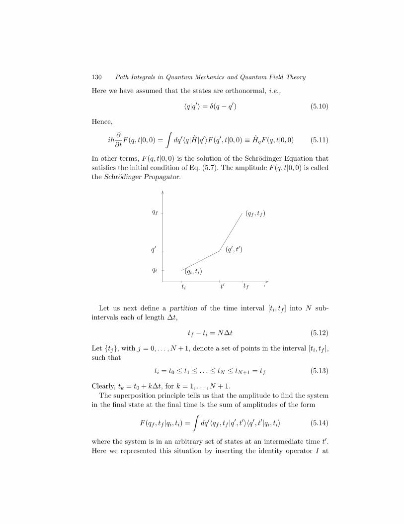
In other terms, F (q, t|0, 0) is the solution of the Schrodinger Equation thatsatisfies the initial condition of Eq. (5.7). The amplitude F (q, t|0, 0) is calledthe Schrodinger Propagator.
t
qf
qi
q′
ti t′ tf
(q′, t′)
(qi, ti)
(qf , tf )
Let us next define a partition of the time interval [ti, tf ] into N sub-intervals each of length ∆t,
tf − ti = N∆t (5.12)
Let {tj}, with j = 0, . . . , N +1, denote a set of points in the interval [ti, tf ],such that
ti = t0 ≤ t1 ≤ . . . ≤ tN ≤ tN+1 = tf (5.13)
Clearly, tk = t0 + k∆t, for k = 1, . . . , N + 1.The superposition principle tells us that the amplitude to find the system
in the final state at the final time is the sum of amplitudes of the form
F (qf , tf |qi, ti) =∫
dq′⟨qf , tf |q′, t′⟩⟨q′, t′|qi, ti⟩ (5.14)
where the system is in an arbitrary set of states at an intermediate time t′.Here we represented this situation by inserting the identity operator I at

5.1 Path Integrals and Quantum Mechanics 131
the intermediate time t′ in the form of the resolution of the identity of Eq.(5.14). By repeating this process many times we find
F (qf , tf |qi, ti) =∫
dq1 . . . dqN ⟨qf , tf |qN , tN ⟩⟨qN , tN |qN−1, tN−1⟩ × . . .
× . . . ⟨qj, tj |qj−1, tj−1⟩ . . . ⟨q1, t1|qi, ti⟩ (5.15)
Each factor ⟨qj , tj |qj−1, tj−1⟩ in Eq.(5.15) has the form
⟨qj , tj |qj−1, tj−1⟩ = ⟨qj|e−iH(tj−tj−1)/!|qj−1⟩ ≡ ⟨qj |e−iH∆t/!|qj−1⟩ (5.16)
In the limit N →∞, with |tf − ti| fixed and finite, the interval ∆t becomesinfinitesimally small and ∆t → 0. Hence, as N → ∞ we can approximatethe expression for ⟨qj, tj |qj−1, tj−1⟩ in Eq.(5.16) as follows
⟨qj, tj |qj−1, tj−1⟩ = ⟨qj|e−iH∆t/!|qj−1⟩
= ⟨qj|{I − i
∆t
!H +O((∆t)2)
}|qj−1⟩
= δ(qj − qj−1)− i∆t
!⟨qj|H |qj−1⟩+O((∆t)2)
(5.17)
which becomes asymptotically exact as N →∞.
ttiti ∆t
q(t)
qf
qi q(ti) = qi
q(tf ) = qf
Figure 5.1 A history q(t) of the system.
We can also introduce at each intermediate time tj a complete set ofmomentum eigenstates {|p⟩} and their resolution of the identity
I =
∫ ∞
−∞dp |p⟩⟨p| (5.18)
132 Path Integrals in Quantum Mechanics and Quantum Field Theory
Recall that the overlap between the states |q⟩ and |p⟩ is
⟨q|p⟩ = 1√2π!
eipq/! (5.19)
For a typical Hamiltonian of the form
H =p2
2m+ V (q) (5.20)
its matrix elements are
⟨qj|H|qj−1⟩ =∫ ∞
−∞
dpj2π!
eipj(qj−qj−1)/!
[p2j2m
+ V (qj)
](5.21)
Within the same level of approximation we can also write
⟨qj , tj|qj−1, tj−1⟩ ≈∫
dpj2π!
exp
[i
(pj!(qj − qj−1)−∆t H
(pj,
qj + qj−1
2
))]
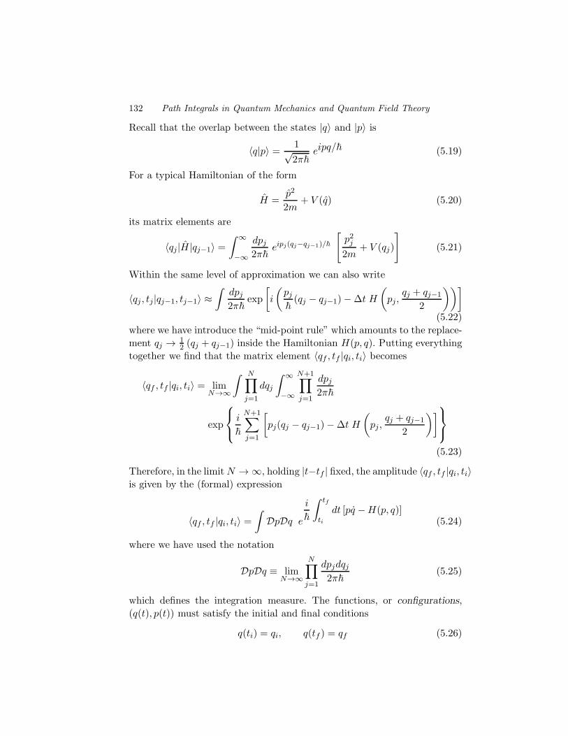
(5.22)where we have introduce the “mid-point rule” which amounts to the replace-ment qj → 1
2 (qj + qj−1) inside the Hamiltonian H(p, q). Putting everythingtogether we find that the matrix element ⟨qf , tf |qi, ti⟩ becomes
⟨qf , tf |qi, ti⟩ = limN→∞
∫ N∏
j=1
dqj
∫ ∞
−∞
N+1∏
j=1
dpj2π!
exp
⎧⎨
⎩i
!
N+1∑
j=1
[pj(qj − qj−1)−∆t H
(pj,
qj + qj−1
2
)]⎫⎬
⎭
(5.23)
Therefore, in the limitN →∞, holding |t−tf | fixed, the amplitude ⟨qf , tf |qi, ti⟩is given by the (formal) expression
⟨qf , tf |qi, ti⟩ =∫
DpDq e
i
!
∫ tf
ti
dt [pq −H(p, q)](5.24)
where we have used the notation
DpDq ≡ limN→∞
N∏
j=1
dpjdqj2π!
(5.25)
which defines the integration measure. The functions, or configurations,(q(t), p(t)) must satisfy the initial and final conditions
q(ti) = qi, q(tf ) = qf (5.26)
5.1 Path Integrals and Quantum Mechanics 133
Thus the matrix element ⟨qf , tf |qi, ti⟩ can be expressed as a sum over histo-ries in phase space. The weight of each history is the exponential factor ofEq. (5.24). Notice that the quantity in brackets it is just the Lagrangian
L = pq −H(p, q) (5.27)
Thus the matrix element is just
⟨qf , tf |q, t⟩ =∫
DpDq ei!S(q,p) (5.28)
where S(q, p) is the action of each history (q(t), p(t)). Also notice that thesum (or integral) runs over independent functions q(t) and p(t) which are notrequired to satisfy any constraint (apart from the initial and final conditions)and, in particular they are not the solution of the equations of motion.Expressions of these type are known as path-integrals. They are also calledfunctional integrals, since the integration measure is a sum over a space offunctions, instead of a field of numbers as in a conventional integral.
Using a Gaussian integral of the form (which involves an analytic contin-uation)
∫ ∞
−∞
dp
2π!ei(pq − p2
2m)∆t
! =
√m
2πi!∆tei∆t
2!q2
(5.29)
we can integrate out explicitly the momenta in the path-integral and find aformula that involves only the histories of the coordinate alone. (Notice thatthere are no initial and final conditions on the momenta since the initial andfinal states have well defined positions.) The result is
⟨qf , tf |qi, ti⟩ =∫
Dq e
i
!
∫ tf
ti
dt L(q, q)(5.30)
which is known as the Feynman Path Integral. Here L(q, q) is
L(q, q) =1
2mq2 − V (q) (5.31)
and the sum over histories q(t) is restricted by the boundary conditionsq(ti) = qi and q(tf ) = qf .
Notice now that the Feynman path-integral tells us that in the correspon-dence limit ! → 0, the only history (or possibly histories) that contributesignificantly to the path integral must be those that leave the action Sstationary since, otherwise, the contributions of the rapidly oscillating ex-ponential would add up to zero. In other words, in the classical limit thereis only one history qc(t) that contributes. For this history, qc(t), the action

134 Path Integrals in Quantum Mechanics and Quantum Field Theory
q
q(ti)
q(tf )
tti tf
Figure 5.2 Two histories with the same initial and final states.
S is stationary, δS = 0, and qc(t) is the solution of the Classical Equationof Motion
∂L
∂q− d
dt
∂L
∂q(5.32)
In other terms, in the correspondence limit ! → 0, the evaluation of theFeynman path integral reduces to the requirement that the Least ActionPrinciple should hold. We are in the classical limit.
5.2 Evaluating Path Integrals in Quantum Mechanics
Let us first discuss the following problem. We wish to know how to computethe amplitude ⟨qf , tf |qi, ti⟩ for a dynamical system whose Lagrangian hasthe standard form of Eq. (5.31). For simplicity we will begin with a linearharmonic oscillator.
The Hamiltonian for a linear harmonic oscillator is
H =p2
2m+
mω2
2q2 (5.33)
and the associated Lagrangian is
L =m
2q2 − mω2
2q2 (5.34)
Let qc(t) be the classical trajectory. It is the solution of the classical equa-tions of motion
d2qcdt2
+ ω2qc = 0 (5.35)
Let us denote by q(t) an arbitrary history of the system and by ξ(t) its

5.2 Evaluating Path Integrals in Quantum Mechanics 135
deviation from the classical solution qc(t). Since all the histories, includingthe classical trajectory qc(t), obey the same initial and final conditions
q(ti) = qi q(tf ) = qf (5.36)
it follows that ξ(t) obeys instead vanishing initial and final conditions:
ξ(ti) = ξ(tf ) = 0 (5.37)
After some trivial algebra it is easy to show that the action S for an arbitraryhistory q(t) becomes
S(q, q) = S(qc, qc)+S(ξ, ξ)+
∫ tf
ti
dtd
dt
[mξ
dqcdt
]+
∫ tf
ti
dt mξ
(d2qcdt2
+ ω2qc
)
(5.38)The third term vanishes due to the boundary conditions obeyed by thefluctuations ξ(t), Eq. (5.37). The last term also vanishes since qc is a solutionof the classical equation of motion Eq. (5.35). These two features hold forall systems, even if they are not harmonic. However, the Lagrangian (andhence the action) for ξ, the second term in Eq. (10.4), in general is not thesame as the action for the classical trajectory (the first term). Only for theharmonic oscillator S(ξ, ξ) has the same form as S(qc, qc).
Hence, for a harmonic oscillator we get
⟨qf , tf |qi, ti⟩ = ei!S(qc,qc)
∫
ξ(ti)=ξ(tf )=0Dξ e
i!
! tfti
dtL(ξ,ξ) (5.39)
Notice that the information on the initial and final states enters only throughthe factor associated with the classical trajectory. For the linear harmonicoscillator, the quantum mechanical contribution is independent of the initialand final states. Thus, we need to do two things: 1) we need an explicit solu-tion qc(t) of the equation of motion, for which we will compute S(qc, qc), and2) we need to compute the quantum mechanical correction, the last factorin Eq. (5.39), which measures the strength of the quantum fluctuations.
For a general dynamical system, whose Lagrangian has the form of Eq.(5.31), the action of Eq. (10.4) takes the form
S(q, q) = S(qc, qc) + Seff(ξ, ξ; qc)
+
∫ tf
ti
dtd
dt
[mξ
dqcdt
]+
∫ tf
ti
dt
(
md2qcdt2
+∂V
∂q
∣∣∣∣qc
)
ξ(t)
(5.40)
where the Seff is the effective action for the fluctuations ξ(t) whose effective
136 Path Integrals in Quantum Mechanics and Quantum Field Theory
Lagrangian Leff(ξ, ξ; qc) is
Leff(ξ, ξ) =1
2mξ2 − 1
2
∂2V
∂q2
∣∣∣∣qc
ξ2 −O(ξ3) (5.41)
Once again, the boundary conditions ξ(ti) = ξ(tf ) = 0 and the fact theqc(t) is a solution of the equation of motion together imply that the last twoterms of Eq. (5.40) vanish identically.
Thus, to the extent that we are allowed to neglect the O(ξ3) (and higher)corrections, the effective Lagrangian Leff can be approximated by a La-grangian which is quadratic in the fluctuation ξ. In general, the effectiveLagrangian will depend on the actual classical trajectory, since V
′′(qc) in
general is not a constant, but a function of time determined by qc(t). How-ever, if one is interested in the quantum fluctuations about a minimum ofthe potential V (q), then qc(t) is constant (and equal to the minimum). Wewill discuss below this case in detail.
Before we embark in an actual computation it is worthwhile to ask whenit should be a good approximation to neglect the terms O(ξ3) (and higher).Since we are expanding about the classical path qc, we expect that thisapproximation should be correct as we formally take the limit !→ 0. In thepath integral the effective action always appears in the combination Seff/!.Hence, for an effective action which is quadratic in ξ, we can eliminate thedependence on ! by the rescaling
ξ =√!ξ (5.42)
This rescaling leaves the classical contribution S(qc)/! unaffected. However,terms with higher powers in ξ, say O(ξn), scale like !n/2. Thus the action(divided by !) has an expansion of the form
S
!=
1
!S(0)(qc) + S(2)(ξ; qc) +
∞∑
n=3
!n/2S(n)(ξ; qc) (5.43)
Thus, in the limit !→ 0, we can expand the weight of the path integral inpowers of !. The matrix element we are calculating then takes the form
⟨qf , tf |qi, ti⟩ = eiS(0)(qc)/! Z(2)(qc) (1 +O(!)) (5.44)
The quantity Z(2)(qc) is the result of keeping only the quadratic approxi-mation. The higher order terms are a power series expansion in ! and areanalytic functions of !. Here I have used the fact that by symmetry theodd powers in ξ in general do not contribute, although there are some caseswhere they do.
5.2 Evaluating Path Integrals in Quantum Mechanics 137
Let us now calculate the effect of the quantum fluctuations to quadraticorder. This is the WKB approximation. Let us denote this factor by Z,
Z(2)(qc) =
∫
ξ(ti)=ξ(tf )=0Dξ ei
! tfti
dt L(2)eff (ξ, ˙ξ;qc) (5.45)
It is elementary to show that, due to the boundary conditions, the actionSeff(ξ, ξ) becomes
Seff(ξ,˙ξ) =
1
2
∫ tf
ti
dt ξ(t)
[−m d2
dt2− V
′′(qc(t))
]ξ(t) (5.46)
The differential operator
A = −m d2
dt2− V
′′(qc(t)) (5.47)
has the form of a Schrodinger operator for a particle on a “coordinate” t ina potential −V ′′
(qc(t)).Let ψn(t) be a complete set of eigenfunctions of A satisfying the boundary
conditions ψ(ti) = ψ(tf ) = 0. Completeness and othonormality implies thatthe eigenfunctions {ψn(t)} satisfy
∑
n
ψ∗n(t)ψn(t
′) = δ(t− t′)
∫ tf
ti
dt ψ∗n(t)ψm(t) = δn,m
(5.48)
An arbitrary function ξ(t) which satisfies the vanishing boundary conditionsof Eq.(5.37) can be expanded as a linear combination of the basis eigenfunc-tions {ψn(t)},
ξ(t) =∑
n
cnψn(t) (5.49)
Clearly, we have ξ(ti) = ξ(tf ) = 0 as we should.For the special case of qi = qf = q0, where q0 is a minimum of the
potential V (q), V ′′(q0) = ωeff > 0 is a constant, and the eigenvectors of theSchrodinger operator are just plane waves. (For a linear harmonic oscillatorωeff = ω.) Thus, in this case the eigenvectors are
ψn(t) = bn sin(kn(t− ti)) (5.50)
where
kn =πn
tf − tin = 1, 2, 3, . . . (5.51)

138 Path Integrals in Quantum Mechanics and Quantum Field Theory
and bn = 1/√
tf − ti. The eigenvalues of A are
An = k2n − ω2eff =
π2
(tf − ti)2n2 − ω2
eff (5.52)
By using the expansion of Eq. (5.49), we find that the action S(2) takes theform
S(2) =1
2
∫ tf
ti
dt ξ(t) A ξ(t) =1
2
∑
n
Anc2n (5.53)
where we have used the completeness and orthonormality of the basis func-tions {ψn(t)}.
The expansion of Eq.(5.49) is a canonical transformation ξ(t)→ cn. Moreto the point, the expansion is actually a parametrization of the possiblehistories in terms of a set of orthonormal functions, and it can be used todefine the integration measure to be
Dξ = N∏
n
dcn√2π
(5.54)
with unit Jacobian. Here N is an irrelevant normalization constant that willbe defined below.
Finally, the (formal) Gaussian integral, which is defined by a suitableanalytic continuation, is
∫ ∞
−∞
dcn√2π
e(i/2)Anc2n = [−iAn]−1/2 (5.55)
can be used to write the amplitude as
Z(2) = N∏
n
A−1/2n ≡ N (DetA)−1/2 (5.56)
where we have used the definition that the determinant of an operator isequal to the product of its eigenvalues. Therefore, up to a normalizationconstant, we obtained the result
Z(2) = (DetA)−1/2 (5.57)
We have thus reduced the problem of the computation of the leading (Gaus-sian) fluctuations to the path-integral to the computation of a determinantof the fluctuation operator, a differential operator defined by the choice ofclassical trajectory. Below you will see how this is done.
It is useful to consider the related problem obtained by an analytic con-tinuation to imaginary time, t→ −iτ . We saw before that there is a relation

5.2 Evaluating Path Integrals in Quantum Mechanics 139
between this problem and Statistical Physics. We will now work out oneexample that will be very instructive.
Formally, upon the analytic continuation t→ −iτ we get
⟨qf |ei
!H(tf − ti)|qi⟩ → ⟨qf |e
−1
!H(τf − τi)|qi⟩ (5.58)
Let us choose
τi = 0 τf = β! (5.59)
where β = 1/T , and T is the temperature (in units of kB = 1). Hence, wefind that
⟨qf ,−iβ/!|qi, 0⟩ = ⟨qf |e−βH |qi⟩ (5.60)
The operator ρ
ρ = e−βH (5.61)
is the Density Matrix in the Canonical Ensemble of Statistical Mechanicsfor a system with Hamiltonian H in thermal equilibrium at temperature T .
It is customary to define the Partition Function Z,
Z = tre−βH ≡∫
dq ⟨q|e−βH |q⟩ (5.62)
where I inserted a complete set of eigenstates of q. Using the results thatwere derived above, we see that the partition function Z can be written asa (Euclidean) Feynman path integral in imaginary time, of the form
Z =
∫Dq[τ ] exp
{−1
!
∫ β!
0dτ
[1
2m
(∂q
∂τ
)2
+ V (q)
]}
≡∫
Dq[τ ] exp
{−∫ β
0dτ
[m
2!2
(∂q
∂τ
)2
+ V (q)
]}(5.63)
where, in the last equality we have rescaled τ → τ/!. Eq. (5.63) is knownas the Feynman-Kac Formula.
Since the Partition Function is a trace over states, we must use boundaryconditions such that the initial and final states are the same state, and tosum over all such states. In other terms, we must have periodic boundaryconditions in imaginary time (PBC’s),i.e.,
q(τ) = q(τ + β) (5.64)
Therefore a quantum mechanical system at finite temperature T can be

140 Path Integrals in Quantum Mechanics and Quantum Field Theory
described in terms of an equivalent system in classical statistical mechanicswith Hamiltonian (or energy)
H =m
2!2
(∂q
∂τ
)2
+ V (q) (5.65)
on a segment of length 1/T and obeying PBC’s. This effectively means thatthe segment is actually a ring of length β = 1/T .
Alternatively, upon inserting a complete set of eigenstates of the Hamilto-nian, it is easy to see that an arbitrary matrix element of the density matrixhas the form
⟨q′|e−βH |q⟩ =∞∑
n=0
⟨q′|n⟩⟨n|q⟩e−βEn
=∞∑
n=0
e−βEnψ∗n(q
′)ψn(q) −−−−→β →∞
e−βE0ψ∗0(q
′)ψ0(q)
(5.66)
where {En} are the eigenvalues of the Hamiltonian, E0 is the ground stateenergy and ψ0(q) is the ground state wave function.
Therefore, we can calculate both the ground state energy E0 and theground state wave function from the density matrix and consequently fromthe (imaginary time) path integral. For example, from the identity
E0 = − limβ→∞
1
βln tre−βH (5.67)
we see that the ground state energy is given by
E0 = − limβ→∞
1
βln
∫
q(0)=q(β)Dq exp
{−∫ β
0dτ
[m
2!2
(∂q
∂τ
)2
+ V (q)
]}
(5.68)Mathematically, the imaginary time path integral is a better behaved objectthan its real time counterpart, since it is a sum of positive quantities, thestatistical weights. In contrast, the Feynman path integral (in real time)is a sum of phases and as such it is an ill-defined object. It is actuallyconditionally convergent and to make sense of it convergence factors (orregulators) will have to be introduced. The effect of these convergence factorsis actually an analytic continuation to imaginary time. We will encounter thesame problem in the calculation of propagators. Thus, the imaginary timepath integral, often referred to as the Euclidean path integral (as opposed toMinkowski), can be used to describe both a quantum system and a statisticalmechanics system.
5.2 Evaluating Path Integrals in Quantum Mechanics 141
Finally, we notice that at low temperatures T → 0, the Euclidean PathIntegral can be approximated using methods similar to the ones we discussedfor the (real time) Feynman Path Integral. The main difference is that wemust sum over trajectories which are periodic in imaginary time with periodβ = 1/T . In practice this sum can only be done exactly for simple systemssuch as the harmonic oscillator, and for more general systems one has toresort to some form of perturbation theory. Here we will consider a physicalsystem described by a dynamical variable q and a potential energy V (q)which has a minimum at q0 = 0. For simplicity we will take V (0) = 0and we will denote by mω2 = V
′′(0) (in other words, an effective harmonic
oscillator). The partition function is given by the Euclidean path integral
Z =
∫Dq[τ ] exp
{−1
2
∫ β
0ξ(τ)AEξ(τ)dτ
](5.69)
where AE is the imaginary time, or Euclidean, version of the operator A,and it is given by
AE = −m
!2
d2
dτ2+ V
′′(qc(τ)) (5.70)
The functions this operator acts on obey periodic boundary conditions withperiod β. Notice the important change in the sign of the term of the poten-tial. Hence, once again we will need to compute a functional determinant,although the operator now acts on functions obeying periodic boundary con-ditions. In a later chapter we will see that in the case of fermionic theories,the boundary conditions become antiperiodic.
5.2.1 Computation of the Functional Determinant
We will now do the computation of the determinant in Z(2). We will dothe calculation in imaginary time and then we will carry out the analyticcontinuation to real time. We want to compute
D = Det
[−m
!2
d2
dτ2+ V
′′(qc(τ))
](5.71)
subject to the requirement that the space of functions that the operatoracts on obeys specific boundary conditions in (imaginary) time. We will beinterested in two cases: (a) Vanishing Boundary Conditions (VBC’s), whichare useful to study quantum mechanics at T = 0, and (b) Periodic Bound-ary Conditions (PBC’s) with period β = 1/T . The approach is somewhatdifferent in the two situations.
142 Path Integrals in Quantum Mechanics and Quantum Field Theory
Vanishing Boundary Conditions
This method is explained in detail in Sidney Coleman’s book, Aspects of
Symmetry. I will follow his approach closely.We define the (real) variable x = !
mτ . The range of x is the interval [0, L],with L = !β/
√m. Let us consider the following eigenvalue problem for the
Schrodinger operator −∂2 +W (x), i.e.,(−∂2 +W (x)
)ψ(x) = λψ(x) (5.72)
subject to the boundary conditions ψ(0) = ψ(L) = 0. Formally, the deter-minant is given by
D =∏
n
λn (5.73)
where {λn} is the spectrum of eigenvalues of the operator −∂2 +W (x) fora space of functions satisfying a given boundary condition.
Let us define an auxiliary function ψλ(x), with λ a real number not neces-sarily in the spectrum of the operator, such that the following requirementsare met:
1 ψλ(x) is a solution of Eq. (8.143), and2 ψλ obeys the initial conditions, ψλ(0) = 0 and ∂xψλ(0) = 1.
It is easy to see that −∂2 + W (x) has an eigenvalue at λn if and onlyif ψλn(L) = 0. (Because of this property this procedure is known as theShooting Method.) Hence, the determinant D of Eq. (5.73) is equal to theproduct of the zeros of ψλ(x) at x = L.
Consider now two potentials W (1) and W (2), and the associated functions,ψ(1)λ (x) and ψ(2)
λ (x). Let us show that
Det[−∂2 +W (1)(x)− λ
]
Det[−∂2 +W (2)(x)− λ
] =ψ(1)λ (L)
ψ(2)λ (L)
(5.74)
The l. h. s. of Eq. (5.74) is a meromorphic function of λ in the complexplane, which has simple zeros at the eigenvalues of −∂2+W (1)(x) and simplepoles at the eigenvalues of −∂2 + W (2)(x). Also, the l. h. s. of Eq. (5.74)approaches 1 as |λ|→∞, except along the positive real axis which is wherethe spectrum of eigenvalues of both operators is. Here we have assumed thatthe eigenvalues of the operators are non-degenerate, which is the generalcase. Similarly, the r. h. s. of Eq. (5.74) is also a meromorphic function of λ,which has exactly the same zeros and the same poles as the l. h. s. . It alsogoes to 1 as |λ| → ∞ (again, except along the positive real axis), since thewave-functions ψλ are asymptotically plane waves in this limit . Therefore,

5.2 Evaluating Path Integrals in Quantum Mechanics 143
the function formed by taking the ratio r. h. s. / l. h. s. is an analytic functionon the entire complex plane and it approaches 1 as |λ|→∞. Then, generaltheorems of the Theory of Functions of a Complex Variable tell us that thisfunction is equal to 1 everywhere.
From these considerations we conclude that the following ratio is inde-pendent of W (x),
Det(−∂2 +W (x)− λ
)
ψλ(L)(5.75)
We now define a constant N such that
Det(−∂2 +W (x)
)
ψ0(L)= π!N 2 (5.76)
Then, we can write
N[Det
(−∂2 +W
)]−1/2= [π!ψ0(L)]
−1/2 (5.77)
Thus we reduced the computation of the determinant (including the normal-ization constant) to finding the function ψ0(L). For the case of the linearharmonic oscillator, this function is the solution of
[− ∂2
∂x2+mω2
]ψ0(x) = 0 (5.78)
with the initial conditions, ψ0(0) = 0 and ψ′0(0) = 1. The solution is
ψ0(x) =1√mω
sinh(√mωx) (5.79)
Hence,
Z = N[Det
(− ∂2
∂x2+mω2
)]−1/2
= [π!ψ0(L)]−1/2 (5.80)
and we find
Z =
[π!√mω
sinh(βω)
]−1/2
(5.81)
where we have used L == !β/√m. From this result we find that the ground
state energy is
E0 = limβ→∞
−1β
lnZ =!ω
2(5.82)
as it should be.Finally, by means of an analytic continuation back to real time, we can

144 Path Integrals in Quantum Mechanics and Quantum Field Theory
use these results to find, for instance, the amplitude to return to the originafter some time T . Thus, for tf − ti = T and qf = qi = 0, we get
⟨0, T |0, 0⟩ =[
iπ!√mω
sin(ωT )
]−1/2
(5.83)
Periodic Boundary Conditions
Periodic boundary conditions imply that the histories satisfy q(τ) = q(τ+β).Hence, these functions can be expanded in a Fourier series of the form
q(τ) =∞∑
n=−∞
eiωnτqn (5.84)
where ωn = 2πn/β. Since q(τ) is real, we have the constraint q−n = q∗n. Forsuch configurations (or histories) the action becomes
S =
∫ β
0dτ
[m
2!2
(∂q
∂τ
)2
+1
2V
′′(0)q2
]
=β
2V
′′(0)q20 + β
∑
n≥1
[m!2ω2n + V
′′(0)]|qn|2 (5.85)
The integration measure now is
Dq[τ ] = N dq0√2π
∏
n≥1
dReqn dImqn2π
(5.86)
where N is a normalization constant that will be discussed below. Afterdoing the Gaussian integrals, the partition function becomes,
Z = N 1√βV ′′(0)
∏
n≥1
1βm!2ω2n + βV ′′(0)
= N[
∞∏
n=−∞
1βm!2ω2n + βV ′′(0)
]1/2
(5.87)Formally, the infinite products that enter in this equation are divergent. Thenormalization constant N eliminates this divergence. This is an example ofwhat is called a regularization. The regularized partition function is
Z =
√m
!2β
1√βV ′′(0)
∏
n≥1
[
1 +!2V
′′(0)
mω2n
]−1
(5.88)
Using the identity∏
n≥1
(1 +
a2
n2π2
)=
sinh a
a(5.89)
5.3 Path Integrals for a Scalar Field Theory 145
we find
Z =1
2 sinh
⎛
⎝β!2
(V
′′(0)
m
)1/2⎞
⎠
(5.90)
which is the standard partition function for a linear harmonic oscillator, seeL. D. Landau and E. M. Lifshitz, Statistical Physics.
5.3 Path Integrals for a Scalar Field Theory
We will now develop the path-integral quantization picture for a scalar fieldtheory. Our starting point will be the canonically quantized scalar field. Aswe saw before in canonical quantization the scalar field φ(x) is an operatorthat acts on a Hilbert space of states. We will use the field representation,which is the analog of the conventional coordinate representation in Quan-tum Mechanics. Thus, the basis states are labelled by the field configurationat some fixed time x0, i.e., a set of states of the form { |{φ(x, x0)}⟩ }. Thefield operator φ(x, x0) acts trivially on these states,
φ(x, x0)|{φ(x, x0)}⟩ = φ(x, x0)|{φ(x, x0)}⟩ (5.91)
The set of states { |{φ(x, x0)}⟩ } is both complete and orthonormal. Com-pleteness here means that these states span the entire Hilbert space. Con-sequently the identity operator I in the full Hilbert space can be expandedin a complete basis in the usual manner, which for this basis it means
I =
∫Dφ(x, x0) |{φ(x, x0)}⟩⟨{φ(x, x0)}| (5.92)
Notice that since the completeness condition involves a sum over all thestates in the basis and since this basis is the set of field configurations ata given time x0, we will need to give a definition for integration measurewhich represents the sums over the field configurations. In this case there isa trivial definition,
Dφ(x, x0) =∏
x
dφ(x, x0) (5.93)
Likewise, othonormality of the basis states is the condition
⟨φ(x, x0)|φ′(x, x0)⟩ =∏
x
δ(φ(x, x0)− φ′(x, x0)
)(5.94)
Thus, we have a working definition of the Hilbert space for a real scalarfield. Naturally, there are many other definitions of this Hilbert space andthey are all equally good.

146 Path Integrals in Quantum Mechanics and Quantum Field Theory
We saw in the previous section that in canonical quantization the classicalcanonical momentum Π(x, x0), defined as
Π(x, x0) =δL
δ∂0φ(x, x0)= ∂0φ(x, x0) (5.95)
becomes an operator that acts on the same Hilbert space as the field itself φdoes. The field φ and the canonical momentum π satisfy equal time canonical
commutation relations[φ(x, x0), Π(y, x0)
]= i!δ3(x− y) (5.96)
Here we will use the Lagrangian density for a real scalar field
L =1
2(∂µφ)
2 − V (φ) (5.97)
It is a simple matter to generalize what follows below to more general cases,such as complex fields and/or several components. Let us also recall thatthe Hamiltonian for a scalar field is given by
H =
∫d3x
[Π2
2+
1
2
(▽φ
)2+ V (φ)
]
(5.98)
For reasons that will become clear soon, it is convenient to add an extraterm to the Lagrangian density of the scalar field, Eq. (5.97), of the form
Lsource = J(x) φ(x) (5.99)
The field J(x) is called an external source and represents the effects of exter-nal sources on the scalar field. The field J(x) is the analog of external forcesacting on a system of classical particles. Here we will always assume that thesources J(x) vanish both at spacial infinity (at all times) and everywhere inboth the remote past and in the remote future,
lim|x|→∞
J(x, x0) = 0 limx0→±∞
J(x, x0) = 0 (5.100)
The total Lagrangian density is
L(φ, J) = L+ Lsource (5.101)
Notice that since the source J(x) is generally a function of space and time,the Hamiltonian that follows from this Lagrangian is formally time-dependent.
We will derive the path integral for this quantum field theory by followingthe same procedure we used for the case of a finite quantum mechanicalsystem. Hence we begin by considering the amplitude
J⟨{φ(x, x0)}|{φ′(y, y0)}⟩J (5.102)

5.3 Path Integrals for a Scalar Field Theory 147
In other words, we want the amplitude in the background of the sourcesJ(x). We will be interested in situations in which x0 is in the remote futureand y0 is in the remote past. It turns out that this amplitude is intimatelyrelated to the computation of ground state (or vacuum) expectation valuesof time ordered products of field operators in the Heisenberg representation
G(N)(x1, . . . , xN ) ≡ ⟨0|T [φ(x1) . . . φ(xN )]|0⟩ (5.103)
which are the N -point functions (or correlators). In particular the 2-pointfunction
G(2)(x1 − x2) ≡ −i⟨0|T [φ(x1)φ(x2)]|0⟩ (5.104)
is known as the Feynman Propagator for this theory. We will see later on thatall quantities of physical interest can be obtained from a suitable correlationfunction of the type of Eq. (5.103).
In Eq. (5.103) we have use the notation T [φ(x1) . . . φ(xN )] for the time-
ordered product of Heisenberg field operators. For any pair Heisenberg ofoperators A(x) and B(y), (which commute for space-like separations) thetime ordered product is defined to be
T [A(x)B(y)] = θ(x0 − y0)A(x)B(y) + θ(y0 − x0)B(y)A(x) (5.105)
where θ(x) is the step (or Heaviside) function
θ(x) =
{1 if x ≥ 0,
0 otherwise(5.106)
This definition is generalized by induction to to the product of any num-ber of operators. Notice that inside a time-ordered product the Heisenbergoperators behave as numbers.
Let us now recall the structure of the derivation that we gave of the pathintegral in Quantum Mechanics. We will paraphrase that derivation for thisfield theory. We considered an amplitude equivalent to Eq. (5.102), andrealized that this amplitude is actually a matrix element of the evolutionoperator,
J⟨{φ(x, x0)}|{φ′(y, y0)}⟩J = ⟨{φ(x)}|T e− i
!
∫ x0
y0
dx′0 H(x′0)|{φ′(y)}⟩
(5.107)where T stands for the time ordering symbol (not temperature!), and H(x′0)
148 Path Integrals in Quantum Mechanics and Quantum Field Theory
is the time-dependent Hamiltonian whose Hamiltonian density is
H(x0) =1
2Π2(x, x0) +
1
2
(▽φ(x, x0)
)2+ V (φ(x, x0))− J(x, x0)φ(x, x0)
(5.108)We then partitioned the time interval in a large number of steps of width
∆t and inserted a complete set of eigenstates of the field operator φ, sinceit plays the role of the coordinate. As it turned out, we also had to insertcomplete sets of eigenstates of the canonical momentum operator, whichhere means the operator Π(x). The result is the phase-space path integral
J⟨{φ(x, x0)}|{φ′(y, y0)}⟩J =
∫
b. c.DφDΠ e
i
!
∫d4x
[φΠ−H(φ,Π) + Jφ
]
(5.109)where b.c. indicates the boundary conditions required by the requirementthat the initial and final states be |{φ(x, x0)}⟩ and |{φ′(y, y0)}⟩ respectively.
Exactly as in the case of the path integral for a particle, this theoryhas a Hamiltonian quadratic in the momenta Π(x). Hence, we can furtherintegrate out the field Π(x), and obtain the Feynman path integral for thescalar field theory in the form of a sum over histories of field configurations:
J⟨{φ(x, x0)}|{φ′(y, y0)}⟩J = N∫
b. c.Dφ e
i
!S(φ, ∂µφ, J)
(5.110)
where N is an (unimportant) normalization constant, and S(φ, ∂µφ, J) isthe action for a real scalar field φ(x) coupled to a source J(x),
S(φ, ∂µφ, J) =
∫d4x
[1
2(∂µφ)
2 − V (φ) + Jφ
](5.111)
5.4 Path Integrals and Propagators
In Quantum Field Theory we will be interested in calculating vacuum (i.e.ground state) expectation values of field operators at various space-timelocations. Thus, instead of the amplitude J⟨{φ(x, x0)}|{φ′(y, y0)}⟩J we maybe interested in a transition between an initial state, at y0 → −∞ which isthe vacuum state |0⟩, i.e., the ground state of the scalar field in the absenceof the source J(x), and a final state at x0 → ∞ which is also the vacuumstate of the theory in the absence of sources. We will denote this matrixelement by
Z[J ] = J⟨0|0⟩J (5.112)
This matrix element is called the Vacuum Persistence Amplitude.

5.4 Path Integrals and Propagators 149
Let us see now how the vacuum persistence amplitude is related to theFeynman path integral for a scalar field of Eq. (5.110). In order to do thatwe will assume that the source J(x) is “on” between times t < t′ and thatwe watch the system on a much longer time interval T < t < t′ < T ′. Forthis interval, we can now use the Superposition Principle to insert completesets of states at intermediate times t and t′, and write the amplitude in theform
J⟨{Φ′(x, T ′)}|{Φ(x, T )}⟩J = (5.113)∫
Dφ(x, t) Dφ′(x, t′)⟨{Φ′(x, T ′)}|{φ′(x, t′)}⟩
×J⟨{φ′(x, t′)}|{φ(x, t)}⟩J ⟨{φ(x, t)}|{Φ(x, T )}⟩
The matrix elements ⟨{Φ′(x, T ′)}|{φ′(x, t′)}⟩ and ⟨{φ(x, t)}|{Φ(x, T )}⟩ aregiven by
⟨{φ(x, t)}|{Φ(x, T )}⟩ =∑
m
Ψm[{φ(x)}]Ψ∗m[{Φ(x)}] e−iEn(t− T )/!
⟨{Φ′(x, T ′)}|{φ′(x, t′)}⟩ =∑
n
Ψn[{Φ′(x)}]Ψ∗n[{φ′(x)}] e−iEn(T
′ − t′)/!
(5.114)
where we have introduced complete sets of eigenstates |{Ψn}⟩ of the Hamil-tonian of the scalar field (without sources) and the corresponding wave func-tions, {Ψn[Φ(x)]}.
We now analytically continue T along the positive imaginary time axis,and T ′ along the negative imaginary time axis, as shown in figure 5.3. Aftercarrying out the analytic continuation, we find that the following identitieshold,
limT→+i∞
e−iE0T/!⟨{φ(x, t)}|{Φ(x, T )}⟩ = Ψ0[{φ}] Ψ∗0[{Φ}] e−iE0t/!
limT ′→−i∞
eiE0T′/!⟨{Φ′(x, T ′)}|{φ(x, t′)}⟩ = Ψ0[{Φ′}] Ψ∗
0[{φ′}] eiE0t′/!
(5.115)
This result is known as the Gell-Mann-Low Theorem.In this limit all other terms drop out provided the vacuum state |0⟩ is
non-degenerate. This also can be done by lifting a possible degeneracy byan infinitesimally weak external perturbation which is switched off after theinfinite time limit is taken. We will encounter similar issues in our discussionof spontaneous symmetry breaking in later chapters.

150 Path Integrals in Quantum Mechanics and Quantum Field Theory
Re t
Im t
t
T
t′
T ′
Figure 5.3 Analytic continuation.
Hence, in the same limit, we also find the following relation
limT→+i∞
limT ′→−i∞
⟨{Φ′(x, T ′)}|Φ(x, T )}⟩exp [−iE0(T ′ − T )/!] Ψ∗
0[{Φ}] Ψ0[{Φ′}]
=
∫DΦDΦ′ Ψ∗
0[{φ′(x, t′)}] Ψ0[{φ(x, t)}] J⟨{φ′(x, t′)}|{φ(x, t)}⟩J
≡J⟨0|0⟩J (5.116)
Eq.(5.116) gives us a direct relation between the Feynman Path Integral andthe vacuum persistence amplitude of the form
Z[J ] = J⟨0|0⟩J = N limT→+i∞
limT ′→−i∞
∫Dφ e
i
!
∫ T ′
Td4x [L(φ, ∂µφ) + Jφ]
(5.117)In other words, in this asymptotically long time limit, the amplitude ofEq. (5.102) becomes identical to the vacuum persistence amplitude J⟨0|0⟩J ,regardless of the choice of the initial and final states.
Hence we find a direct relation between the vacuum persistence functionZ[J ] and the Feynman Path Integral, given by Eq. (5.117). Notice that inthis limit we can ignore the “hard” boundary condition and work insteadwith free boundary conditions. Or equivalently, physical properties becomeindependent of the initial and final conditions placed. For these reasons,
5.5 Path Integrals in Euclidean space-time and Statistical Physics 151
from now on we will write the simpler expression
Z[J ] = J⟨0|0⟩J = N∫
Dφ e
i
!
∫d4x [L(φ, ∂µφ) + Jφ]
(5.118)
This is a very useful relation. We will see now that Z[J ] is the generatingfunction(al) of all the vacuum expectation values of time ordered productsof fields, i.e. the correlators of the theory.
In particular, let us compute the expression
1
Z[0]
δ2Z[J ]
δJ(x)δJ(x′)
∣∣∣∣J=0
=1
⟨0|0⟩δ2J⟨0|0⟩JδJ(x)δJ(x′)
∣∣∣∣J=0
=
(i
!
)2
⟨0|T [φ(x)φ(x′)]|0⟩
(5.119)Thus, the 2-point function, i.e. the Feynman propagator or propagator of thescalar field φ(x), −i⟨0|T [φ(x)φ(x′)]|0⟩, becomes
⟨0|T [φ(x)φ(x′)]|0⟩ = −i 1
⟨0|0⟩
∫Dφ φ(x) φ(x′) exp
(i
!S[φ, ∂µφ]
)(5.120)
Similarly, the N -point function ⟨0|T [φ(x1) . . . φ(xN )]|0⟩ becomes
⟨0|T [φ(x1) . . . φ(xN )]|0⟩ = (−i!)N 1
⟨0|0⟩δNJ⟨0|0⟩J
δJ(x1) . . . δJ(xN )
∣∣∣∣J=0
=1
⟨0|0⟩
∫Dφ φ(x1) . . . φ(xN ) exp
(i
!S[φ, ∂µφ]
)
(5.121)
where
Z[0] = ⟨0|0⟩ =∫
Dφ exp
(i
!S[φ, ∂µφ]
)(5.122)
Therefore, we find that the Path Integral always yields vacuum expectationvalues of time-ordered products of operators. The quantity Z[J ] can thusbe viewed as the generating functional of the correlation functions of thistheory. These are actually general results that hold for the path integrals ofall theories.
5.5 Path Integrals in Euclidean space-time and Statistical
Physics
In the last section we saw how to relate the computation of transition am-plitudes to path integrals in Minkowski space-time with specific boundaryconditions dictated by the nature of the initial and final states. In particularwe derived explicit expressions for the case of fixed boundary conditions.

152 Path Integrals in Quantum Mechanics and Quantum Field Theory
However we could have chosen other boundary conditions. For instance,for the amplitude to begin in any state at the initial time and to go backto the same state at the final time, but summing over all states. This is thesame as to ask for the trace
Z ′[J ] =
∫DΦJ⟨{Φ(x, t′)}|{Φ(x, t)}⟩J
≡Tr T e− i
!
∫d4x (H − Jφ)
≡∫
PBCDφ e
i
!
∫d4x (L+ Jφ)
(5.123)
where PBC stands for periodic boundary conditions on some generally finitetime interval t′ − t, and T is the time-ordering symbol.
Let us now carry the analytic continuation to imaginary time t→ −iτ , i.e.a Wick Rotation. Upon a Wick rotation the theory has Euclidean invariance,i.e., rotations and translations in D = d+ 1-dimensional space. Imaginarytime plays the same role as the other d spacial dimensions. Hereafter we willdenote imaginary time by xD, and all vectors will have indices µ that runfrom 1 to D.
We will consider two cases: infinite imaginary time interval, and finiteimaginary time interval.
space
imagin
ary
tim
e
β0
Figure 5.4 Periodic boundary conditions wraps space-time into a cylinder.
5.5 Path Integrals in Euclidean space-time and Statistical Physics 153
5.5.1 Infinite Imaginary Time Interval
In this case the path integral becomes
Z ′[J ] =
∫Dφ e
−∫
dDx (LE − Jφ)(5.124)
where D is the total number of space-time dimensions. For the sake of defi-niteness here we are discussing the case D = 4, but the results are obviouslyvalid more generally. Here LE is the Euclidean Lagrangian
LE =1
2(∂0φ)
2 +1
2(▽φ)2 + V (φ) (5.125)
The path integral of Eq. (5.124) has two interpretations.One is simply the infinite time limit (in imaginary time) and therefore it
must be identical to the vacuum persistence amplitude J⟨0|0⟩J . The onlydifference is that from here we get all the N -point functions in Euclideanspace-time (i.e., imaginary time). Therefore, the relativistic interval is
x20 − x2 → −τ2 − x2 < 0 (5.126)
which is always space-like. Hence, with this procedure we will get the correla-tion functions for space-like separations of its arguments. To get to time-likeseparations we will need to do an analytic continuation. This we will dolater on. The second interpretation is that the path integral of Eq. (5.124)is the partition function of a system in Classical Statistical Mechanics in Ddimensions with energy density (divided by T ) equal to LE − Jφ. This willturn out to be a very useful connection (both ways!).
5.5.2 Finite Imaginary Time Interval
In this case we have
0 ≤ x0 = τ ≤ β = 1/T (5.127)
where T will be interpreted as the temperature. Indeed, in this case the pathintegral is
Z ′[0] = Tr e−βH (5.128)
and we are effectively looking at a problem of the same Quantum FieldTheory but at finite temperature T = 1/β. The path integral is once againthe partition function but of a system in Quantum Statistical Physics! The

154 Path Integrals in Quantum Mechanics and Quantum Field Theory
partition function thus is (after setting ! = 1)
Z ′[J ] =
∫Dφ e
−
∫ β
0dτ (LE − Jφ)
(5.129)
where the field φ(x, τ) obeys periodic boundary conditions in imaginarytime,
φ(x, τ) = φ(x, τ + β) (5.130)
This boundary condition will hold for all bosonic theories. We will see lateron that theories with fermions obey instead anti-periodic boundary condi-tions in imaginary time.
Hence, Quantum Field Theory at finite temperature T is just QuantumField Theory on an Euclidean space-time which is periodic (and finite) in onedirection, imaginary time. In other words, we have wrapped (or compactified)Euclidean space-time into a cylinder with perimeter (circumference) β =1/T (in units of ! = kB = 1).
The correlation functions in imaginary time (which we will call the Eu-clidean correlation functions) are given by
1
Z ′[J ]
δNZ ′[J ]
δJ(x1) . . . J(xN )
∣∣∣∣J=0
= ⟨φ(x1) . . . φ(xN )⟩ (5.131)
which are just the correlation functions in the equivalent problem in Statis-tical Mechanics. Upon analytic continuation the Euclidean correlation func-tions ⟨φ(x1) . . . φ(xN )⟩ and the N -point functions of the QFT are relatedby
⟨φ(x1) . . . φ(xN )⟩ ↔ (i!)N ⟨0|Tφ(x1) . . . φ(xN )|0⟩ (5.132)
For the case of a quantum field theory at finite temperature T , the pathintegral yields the correlation functions of the Heisenberg field operatorsin imaginary time. These correlation functions are often called the thermalcorrelation functions (or propagators). They are functions of the spatial po-sitions of the fields, x1, . . . ,xN and of their imaginary time coordinates,xD1, . . . , xDN (here xD ≡ τ). To obtain the correlation functions as a func-tion of the real time coordinates x01, . . . , x0N at finite temperature T it isnecessary to do an analytic continuation. We will discuss how this is donelater on.
5.6 Path Integrals for the Free Scalar Field 155
5.6 Path Integrals for the Free Scalar Field
We will consider now the case of a free scalar field. We will carry our discus-sion in Euclidean space-time (i.e., in imaginary time), and we will do therelevant analytic continuation back to real time at the end of the calculation.
The Euclidean Lagrangian LE for a free field φ coupled to a source J is
LE =1
2(▽µφ)
2 +1
2m2φ2 − Jφ (5.133)
where we are using the notation
(▽µφ)2 = ▽µφ▽µ φ (5.134)
Here the index is µ = 1, . . . ,D for an Euclidean space-time of D = d + 1dimensions. For the most part (but not always) we will be interested in thecase of d = 3 and Euclidean space has four dimensions. Notice the waythe Euclidean space-time indices are placed in Eq. (5.134). This is not amisprint!
We will compute the Euclidean Path Integral (or Partition Function)ZE[J ] exactly. The Euclidean Path Integral for a free field has the form
ZE [J ] = N∫
Dφ e−
∫dDx
[1
2(▽µφ)
2 +1
2m2φ2 − Jφ
]
(5.135)
In Classical Statistical Mechanics this theory is known as the GaussianModel.
In what follows I will assume that the boundary conditions of the fieldφ (and the source J) at infinity are either vanishing or periodic, and thatthe source J also either vanishes at spatial infinity or is periodic. Withthese assumptions all terms which are total derivatives drop out identically.Therefore, upon an integration by parts and after dropping boundary terms,the Euclidean Lagrangian becomes
LE =1
2φ[−▽2 +m2
]φ− Jφ (5.136)
This path integral can be calculated exactly because the action is a quadraticform of the field φ. It has terms which are quadratic (or, rather bilinear) inφ and a term linear in φ, the source term. By means of the following shiftof the field φ
φ(x) = φ(x) + ξ(x) (5.137)
156 Path Integrals in Quantum Mechanics and Quantum Field Theory
the Lagrangian becomes
LE =1
2φ[−▽2 +m2
]φ− Jφ
=1
2φ[−▽2 +m2
]φ− J φ+
1
2ξ[−▽2 +m2
]ξ + ξ
[−▽2 +m2
]φ− Jξ
(5.138)
Hence, we can decouple the source J(x) by requiring that the shift φ be suchthat the terms linear in ξ cancel each other exactly. This requirement leadsto the condition that the classical field φ be the solution of the followinginhomogeneous partial differential equation
[−▽2 +m2
]φ = J(x) (5.139)
Equivalently, we can write the classical field φ is terms of of the source J(x)through the action of the inverse of the operator −▽2 +m2,
φ =1
−▽2 +m2J (5.140)
The solution of Eq. (5.139) is
φ(x) =
∫dDx′ GE
0 (x− x′) J(x′) (5.141)
where
GE0 (x− x′) = ⟨x| 1
−▽2 +m2|x′⟩ (5.142)
is the correlation function of the linear partial differential operator − ▽2
+m2. Thus, GE0 (x− x′) is the solution of
[−▽2
x +m2]GE
0 (x− x′) = δD(x− x′) (5.143)
In terms of GE0 (x− x′), the terms of the shifted action become,
∫dDx
(12φ(x)
[−▽2 +m2
]φ(x)− J φ(x)
)
=− 1
2
∫dDxφ(x)J(x)
=− 1
2
∫dDx dDx′ J(x) GE
0 (x− x′) J(x′)
(5.144)
Therefore the path integral ZE [J ], defined in Eq. (5.135), is given by
ZE [J ] = ZE [0] e
1
2
∫dDx dDx′ J(x) GE
0 (x− x′) J(x′)(5.145)

5.6 Path Integrals for the Free Scalar Field 157
where ZE[0] is
ZE[0] =
∫Dξ e
−1
2
∫dDx ξ(x)
[−▽2 +m2
]ξ(x)
(5.146)
Eq. (5.145) shows that, after the decoupling, ZE[J ] is a product of twofactors: (a) a factor that is function of a bilinear form in the source J , and(b) a path integral, ZE[0], that is independent of the sources.
5.6.1 Calculation of ZE[0]
The path integral ZE [0] is analogous to the fluctuation factor that we foundin the path integral for a harmonic oscillator in elementary quantum me-chanics. There we saw that the analogous factor could be written as a deter-minant of a differential operator, the kernel of the bilinear form that enteredin the action. The same result holds here as well. The only difference is thatthe kernel is now the partial differential operator A = − ▽2 +m2 whereasin Quantum Mechanics is an ordinary differential operator. Here too, theoperator A has a set of eigenstates {Ψn(x)} which, once the boundary con-ditions in space-time are specified, are both complete and orthonormal, andthe associated spectrum of eigenvalues An is
[−▽2 +m2
]Ψn(x) =AnΨn(x)∫
dDx Ψn(x) Ψm(x) =δn,m∑
n
Ψn(x) Ψn(x′) =δ(x− x′) (5.147)
Hence, once again we can expand the field φ(x) in the complete set of states{Ψn(x)}
φ(x) =∑
n
cn Ψn(x) (5.148)
Hence, the field configurations are thus parametrized by the coefficients {cn}.The action now becomes,
S =
∫dDx LE(φ, ∂φ) =
1
2
∑
n
Anc2n (5.149)
Thus, up to a normalization factor, we find that ZE [0] is given by
ZE [0] =∏
n
A−1/2n ≡
(Det
[−▽2 +m2
])−1/2(5.150)

158 Path Integrals in Quantum Mechanics and Quantum Field Theory
Once again, we have reduced the calculation of ZE[0] to the computation ofthe determinant of a differential operator, Det
[−▽2 +m2
].
In chapter 8 we will discuss efficient methods to compute such determi-nants. For the moment it will be sufficient to notice that there is a simple,but formal, way to compute this determinant. First, we notice that if we areinterested in the behavior of of an infinite system at T = 0, the eigenstatesof the operator −▽2 +m2 are simply suitably normalized plane waves. LetL be the linear size of the system (L → ∞). Then the eigenfunctions arelabeled by a D-dimensional momentum pµ (with µ = 0, 1, . . . , d)
Ψp(x) =1
(2πL)D/2ei pµ xµ (5.151)
with eigenvalues,
Ap = p2 +m2 (5.152)
Hence the logarithm of determinant is
lnDet[−▽2 +m2
]= Tr ln
[−▽2 +m2
]
=∑
p
ln(p2 +m2)
= V
∫dDp
(2π)Dln(p2 +m2)
(5.153)
where V = LD is the volume of Euclidean space-time. Hence,
lnZE[0] = −V
2
∫dDp
(2π)Dln(p2 +m2) (5.154)
This expression is has two singularities:
Infrared divergence : It diverges as V → ∞. This infrared (IR) singularityactually is not a problem since lnZE [0] should be an extensive quantitywhich must scale with the volume of space-time. In other words, this is howit should behave.
Ultraviolet divergence : The integral diverges at large momenta unless thereis an upper bound (or cutoff) for the allowed momenta. This is an ultraviolet
(UV) singularity. It has the same origin of the UV divergence of the ground

5.6 Path Integrals for the Free Scalar Field 159
state energy. In fact ZE[0] is closely related to the ground state (vacuum)energy since
ZE [0] = limβ→∞
∑
n
e−βEn ∼ e−βE0 + . . . (5.155)
Thus,
E0 = − limβ→∞
1
βlnZE [0] =
1
2Ld∫
dDp
(2π)Dln(p2 +m2) (5.156)
where Ld is the volume of space, i. e. V = Ldβ. Notice that Eq. (5.156) is UVdivergent. Below in this chapter we will discuss how to compute expressionsof the form of Eq. (5.156).
5.6.2 Propagators and Correlators
A number of interesting results are found immediately by direct inspectionof Eq. (5.145). We can easily see that, once we set J = 0, the correlation
function G(0)E (x− x′)
G(0)E (x− x′) = ⟨x| 1
−▽2 +m2|x′⟩ (5.157)
is equal to the 2-point correlation function for this theory (at J = 0), i.e.,
⟨φ(x)φ(x′)⟩ = 1
ZE[0]
δ2ZE [J ]
δJ(x)δJ(x′)
∣∣∣∣J=0
= G(0)E (x− x′) (5.158)
Likewise we find that, for a free field theory, the N -point correlation function⟨φ(x1) . . . φ(xN )⟩ is equal to
⟨φ(x1) . . . φ(xN )⟩ = 1
ZE [0]
δNZE[J ]
δJ(x1) . . . δJ(xN )
∣∣∣J=0
=⟨φ(x1)φ(x2)⟩ . . . ⟨φ(xN−1)φ(xN )⟩+ permutations
(5.159)
Therefore for a free field, up to permutations of the coordinates x1, . . . , xN ,the N -point functions factorize into products of 2-point functions. Hence, Nmust be an positive even integer. This result, Eq. (12.16), which we derivedin the context of a theory for a free scalar field, is actually much moregeneral. It is known as Wick’s Theorem. It applies to all free theories i.e.,theories whose Lagrangians are bilinear in the fields, it is independent ofthe statistics and on whether there is relativistic invariance or not. The onlycaveat is that, as we will see later on, for the case of fermionic theories thereis a sign associated with each term of this sum.
160 Path Integrals in Quantum Mechanics and Quantum Field Theory
Finally, it is easy to see that, for N = 2k, the total number of terms inthe sum is
(2k − 1)(2k − 3) . . . ... =(2k)!
2kk!(5.160)
Each factor of a 2-point function ⟨φ(x1)φ(x2)⟩, i.e. a free propagator, and itis also called a contraction. It also common to use the notation
⟨φ(x1)φ(x2)⟩ = φ(x1)φ(x2) (5.161)
to denote a contraction or propagator.
5.6.3 Calculation of the Propagator
We will now calculate the 2-point function, or propagator, G(0)E (x − x′) for
infinite Euclidean space. This is the case of interest in QFT at T = 0. Lateron we will do the calculation of the propagator at finite temperature.
Eq. (5.143) tells us that G(0)E (x−x′) is the Green function of the operator
− ▽2 +m2. We will use Fourier transform methods and write G(0)E (x − x′)
in the form
G(0)E (x− x′) =
∫dDp
(2π)DGE
0 (p) ei pµ(xµ − x′µ) (5.162)
which is a solution of Eq. (5.143) if
G(0)E (p) =
1
p2 +m2(5.163)
Therefore the correlation function in real (Euclidean!) space is the integral
G(0)E (x− x′) =
∫dDp
(2π)Dei pµ(xµ − x′µ)
p2 +m2(5.164)
We will often encounter integrals of this type and for that reason we will dothis one in some detail. We begin by using the identity
1
A=
1
2
∫ ∞
0dα e
−A
2α
(5.165)
where A > 0 is a positive real number. The variable α is called a Feynman-Schwinger parameter.
We now choose A = p2 +m2, and substitute this expression back in Eq.(5.164), which takes the form
G(0)E (x− x′) =
1
2
∫ ∞
0dα
∫dDp
(2π)De−α2(p2 +m2) + ipµ(xµ − x′µ)
(5.166)
5.6 Path Integrals for the Free Scalar Field 161
The momentum integrand is now a Gaussian, and the integral can be calcu-lated by a shift of the integration variables pµ, i.e., by completing squares
α
2(p2 +m2)− ipµ(xµ − x′µ) =
1
2
(√αpµ − i
xµ − x′µ√α
)2
− 1
2
(xµ − x′µ√
α
)2
(5.167)and by using the Gaussian integral
∫dDp
(2π)De−1
2
(√αpµ − i
xµ − x′µ√α
)2
= (2πα)−D/2 (5.168)
After all of this is done, we find the formula
G(0)E (x− x′) =
1
2(2π)D/2
∫ ∞
0dα α−D/2 e
− |x− x′|2
2α− 1
2m2α
(5.169)
Let us now define a rescaling of the variable α,
α = λt (5.170)
by which
|x− x′|2
2α+
1
2m2α =
|x− x′|2
2λt+
1
2m2λt (5.171)
We choose
λ =|x− x′|
m(5.172)
With this choice, the exponent becomes
|x− x′|2
2α+
1
2m2α =
m|x− x′|2
(t+
1
t
)(5.173)
After this final change of variables, we find that the correlation function is
G(0)E (x− x′) =
1
(2π)D/2
(m
|x− x′|
)D
2− 1
KD2 −1(m|x− x′|) (5.174)
where Kν(z) is the Bessel function (of imaginary argument, see e.g. Grad-shteyn and Ryzhik) which has the integral representation
Kν(z) =1
2
∫ ∞
0dt tν − 1 e
−z
2
(t+
1
t
)
(5.175)
with ν = D2 − 1, and z = m|x− x′|.
162 Path Integrals in Quantum Mechanics and Quantum Field Theory
power lawdecay decay
exponential
adistanceξ = 1/m
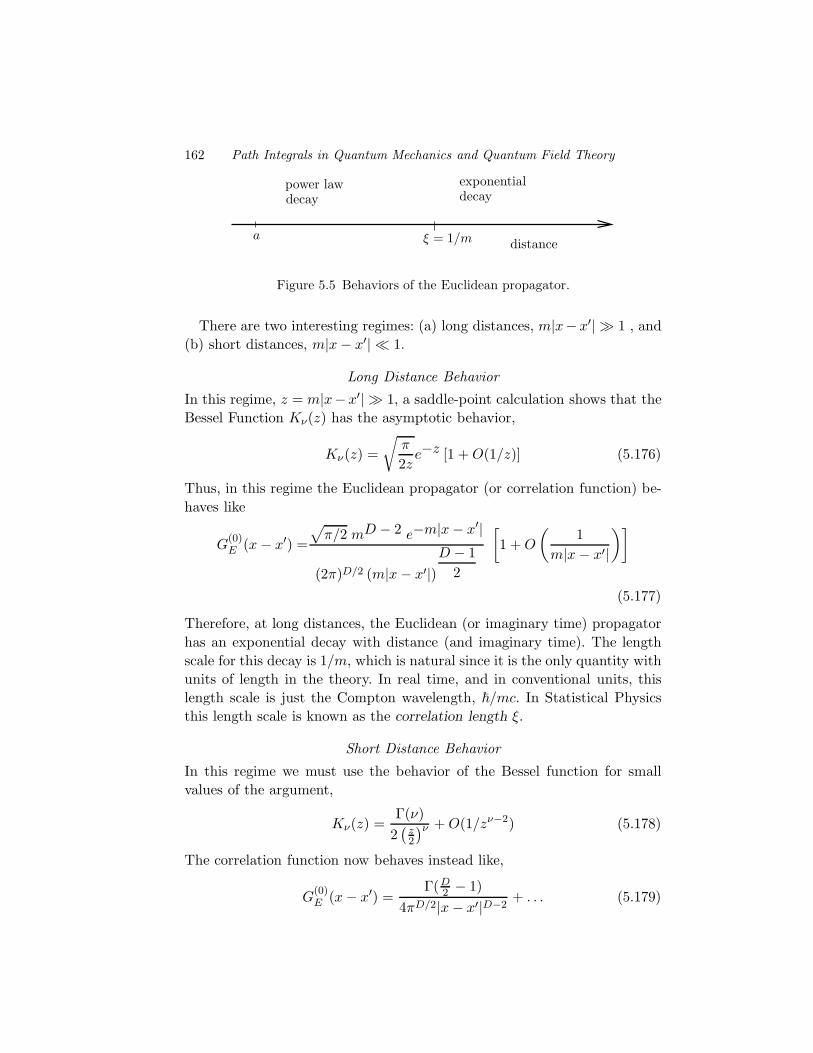
Figure 5.5 Behaviors of the Euclidean propagator.
There are two interesting regimes: (a) long distances, m|x−x′|≫ 1 , and(b) short distances, m|x− x′|≪ 1.
Long Distance Behavior
In this regime, z = m|x−x′|≫ 1, a saddle-point calculation shows that theBessel Function Kν(z) has the asymptotic behavior,
Kν(z) =
√π
2ze−z [1 +O(1/z)] (5.176)
Thus, in this regime the Euclidean propagator (or correlation function) be-haves like
G(0)E (x− x′) =
√π/2 mD − 2 e−m|x− x′|
(2π)D/2 (m|x− x′|)D − 1
2
[1 +O
(1
m|x− x′|
)]
(5.177)
Therefore, at long distances, the Euclidean (or imaginary time) propagatorhas an exponential decay with distance (and imaginary time). The lengthscale for this decay is 1/m, which is natural since it is the only quantity withunits of length in the theory. In real time, and in conventional units, thislength scale is just the Compton wavelength, !/mc. In Statistical Physicsthis length scale is known as the correlation length ξ.
Short Distance Behavior
In this regime we must use the behavior of the Bessel function for smallvalues of the argument,
Kν(z) =Γ(ν)
2(z2
)ν +O(1/zν−2) (5.178)
The correlation function now behaves instead like,
G(0)E (x− x′) =
Γ(D2 − 1)
4πD/2|x− x′|D−2+ . . . (5.179)
5.6 Path Integrals for the Free Scalar Field 163
where . . . are terms that vanish as m|x − x′| → 0. Notice that the leadingterm is independent of the mass m. This is the behavior of the massless
theory.
5.6.4 Behavior of the propagator in Minkowski space
We must now address the issue of the behavior of the propagator in real
time. This means that now we must do the analytic continuation back toreal time x0.
Let us recall that in going from Minkowski to Euclidean space we contin-ued x0 → −ix4. There is also factor of i difference in the definition of thepropagator. Thus, the propagator in Minkowski space-time G(0)(x − x′) isthe expression that results from
G(0)(x− x′) = iG(0)E (x− x′)
∣∣x4→ix0
(5.180)
We can also obtain this result from the path integral formulation inMinkowski space-time. Indeed, the generating functional for a free real mas-sive scalar field Z[J ] in D = d+ 1 dimensional Minkowski space-time is
Z[J ] =
∫Dφe
i
∫dDx
[1
2(∂φ)2 − m2
2φ2 + Jφ
]
(5.181)
Hence, the expectation value to the time-ordered product of two field is
⟨0|Tφ(x)φ(y)|0⟩ = − 1
Z[J ]
δZ[J ]
δJ(x)δJ(y)
∣∣∣J=0
(5.182)
On the other hand, for a free field the generating function is given by (upto a normalization constant N )
Z[J ] = N[Det
(∂2 +m2
)]−1/2e
i
2
∫dDx
∫dDyJ(x)G(0)(x− y)J(y)
(5.183)where G0(x − y) is the Green function of the Klein-Gordon operator andsatisfies
(∂2 +m2
)G(0)(x− y) = δD(x− y) (5.184)
Hence, we obtain the expected result
⟨0|Tφ(x)φ(y)|0⟩ = −iG(0)(x− y) (5.185)
Let us compute the propagator inD = 4Minkowski space-time by analytic
164 Path Integrals in Quantum Mechanics and Quantum Field Theory
continuation from the D = 4 Euclidean propagator. The relativistic intervals is given by
s2 = (x0 − x′0)2 − (x− x
′)2 (5.186)
The Euclidean interval (length) |x − x′|, and the relativistic interval s arerelated by
|x− x′| =√
(x− x′)2 →√−s2 (5.187)
Therefore, in D = 4 space-time dimensions, the Minkowski space propagatoris
G(0)(x− x′) =i
4π2m√−s2
K1(m√−s2) (5.188)
we will need the asymptotic behavior of the Bessel function K1(z),
K1(z) =
√π
2ze−z
[1 +
3
8z+ . . .
], for z ≫ 1
K1(z) =1
z+
z
2
(ln z + C − 1
2
)+ . . . , for z ≪ 1 (5.189)
where C = 0.577215 . . . is the Euler constant. Let us examine the behavior of
space-like separations
time-like separations
Decay Decay
Decay
Oscillatory Behavior
Oscillatory Behavior
Power Law
Exponential Exponential
light cone
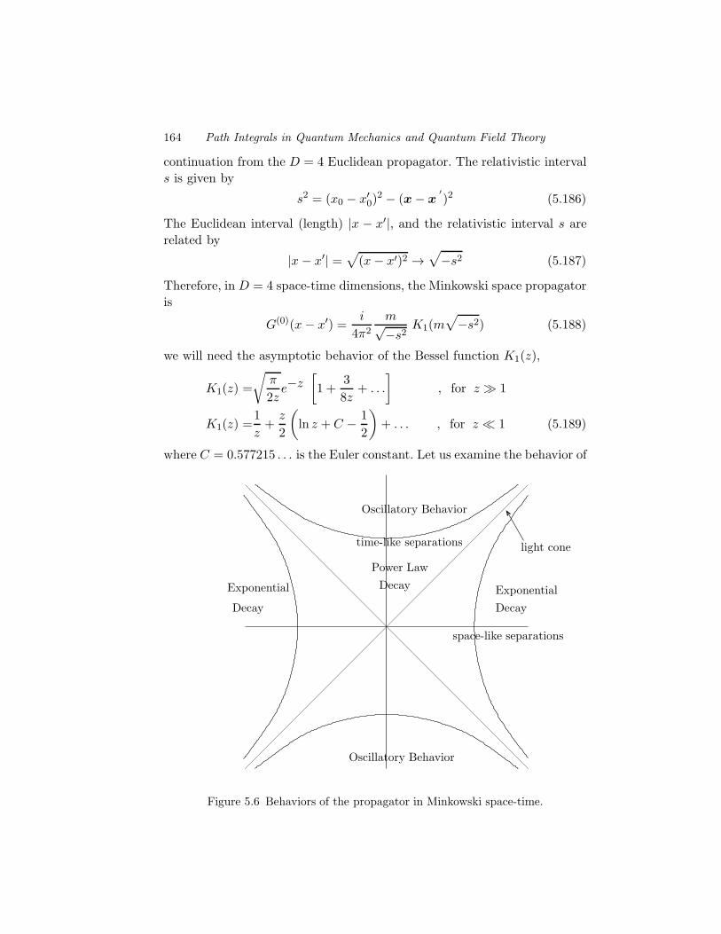
Figure 5.6 Behaviors of the propagator in Minkowski space-time.
5.6 Path Integrals for the Free Scalar Field 165
Eq. (5.188) in the regimes: (a) space-like, s2 < 0, and (b) time-like, s2 > 0,intervals.
Space-like intervals: (x− x′)2 = s2 < 0
This is the space-like domain. By inspecting Eq. (5.188) we see that forspace-like separations, the factor
√−s2 is a positive real number. Conse-
quently the argument of the Bessel function is real (and positive), and thepropagator is pure imaginary. In particular we see that, for s2 < 0 theMinkowski propagator is essentially the Euclidean correlation function,
G(0)(x− x′) = iG(0)E (x− x′) , for s2 < 0 (5.190)
Hence, for s2 < 0 we have the asymptotic behaviors,
G(0)(x− x′) =i
√π/2
4π2m2
(m√−s2
)3/2 e−m
√−s2 , for m
√−s2 ≫ 1
G(0)(x− x′) =i
4π2(−s2) , for m√−s2 ≪ 1
(5.191)
Time-like intervals: (x− x′)2 = s2 > 0
This is the time-like domain. The analytic continuation yields
G(0)(x− x′) =m
4π2√s2
K1(im√s2) (5.192)
For pure imaginary arguments, the Bessel function K1(iz) is the analytic
continuation of the Hankel function,K1(iz) = −π2H
(1)1 (−z) . This function is
oscillatory for large values of its argument. Indeed, we now get the behaviors
G(0)(x− x′) =
√π/2
4π2m2
(m√s2)3/2 e
im√s2 , for m
√s2 ≫ 1
G(0)(x− x′) =1
4π2s2, for m
√s2 ≪ 1 (5.193)
Notice that, up to a factor of i, the short distance behavior is the samefor both time-like and space like separations. The main difference is thatat large time-like separations we get an oscillatory behavior instead of anexponential decay. The length scale of the oscillations is, once again, set bythe only scale in the theory, the Compton wavelength.
166 Path Integrals in Quantum Mechanics and Quantum Field Theory
5.7 Exponential decays and mass gaps
The exponential decay at long space-like separations (and the oscillatorybehavior at long time-like separations) is not a peculiarity of the free fieldtheory. It is a general consequence of the existence of a mass gap in thespectrum. We can see that by considering the 2-point function of a generic
theory, for simplicity in imaginary time. The 2-point function is
G(2)(x− x ′, τ − τ ′) = ⟨0|T φ(x, τ)φ(x ′, τ ′)|0⟩ (5.194)
where T is the imaginary time-ordering operator.The Heisenberg representation of the operator φ in imaginary time is
(! = 1)
φ(x, τ) = eHτ φ(x, 0) e−Hτ (5.195)
Hence, we can write the 2-point function as
G(2)(x− x ′,τ − τ ′) =
= θ(τ − τ ′)⟨0|eHτ φ(x, 0) e−H(τ − τ ′) φ(x ′, 0) e−Hτ′|0⟩
+ θ(τ ′ − τ)⟨0|eHτ′φ(x ′, 0) e−H(τ ′ − τ) φ(x, 0) e−Hτ |0⟩
= θ(τ − τ ′) eE0(τ − τ ′) ⟨0|φ(x, 0) e−H(τ − τ ′) φ(x ′, 0)|0⟩
+ θ(τ ′ − τ) eE0(τ′ − τ) ⟨0|φ(x ′, 0) e−H(τ ′ − τ) φ(x, 0)|0⟩
(5.196)
We now insert a complete set of eigenstates {|n⟩} of the Hamiltonian H,with eigenvalues {En}. The 2-point function now reads,
G(2)(x− x ′,τ − τ ′) =
= θ(τ − τ ′)∑
n
⟨0|φ(x, 0)|n⟩ ⟨n|φ(x ′, 0)|0⟩ e−(En −E0)(τ − τ ′)
+ θ(τ ′ − τ)∑
n
⟨0|φ(x ′, 0)|n⟩ ⟨n|φ(x, 0)|0⟩ e−(En −E0)(τ′ − τ)
(5.197)
Since
φ(x, 0) = eiP · xφ(0, 0)e−iP · x (5.198)
and that
P |0⟩ = 0, P |n⟩ = Pn, (5.199)
5.8 Scalar fields at finite temperature 167
where Pn is the linear momentum of state |n⟩, we can write
⟨0|φ(x, 0)|n⟩ ⟨n|φ(x ′, 0)|0⟩ = |⟨0|φ(0, 0)|n⟩|2 e−iPn · (x− x ′) (5.200)
using the above expressions we can write the expressions in Eq. (5.197) inthe form
G(2)(x− x ′, τ − τ ′)
=∑
n
|⟨0|φ(0, 0)|n⟩|2[θ(τ − τ ′)e−iPn · (x− x ′)e−(En − E0)(τ − τ ′)
+ θ(τ ′ − τ)e−iPn · (x ′ − x)e−(En −E0)(τ′ − τ)
]
(5.201)
Thus, at equal positions, x = x ′, we obtain the simpler expression in theimaginary time interval τ − τ ′
G(2)(0, τ − τ ′) =∑
n
|⟨0|φ(x, 0)|n⟩|2 × e−(En − E0)|τ − τ ′| (5.202)
In the limit of large imaginary time separation, |τ−τ ′|→∞, there is alwaysa largest non-vanishing term in the sums. This is the term for the state |n0⟩that mixes with the vacuum state |0⟩ through the field operator φ, and withthe lowest excitation energy or mass gap En0 −E0. Hence, for |τ − τ ′|→∞,the 2-point function decays exponentially like,
G(2)(0, τ − τ ′) ≃ |⟨0|φ(x, 0)|n0⟩|2 × e−(En0 − E0)|τ − τ ′| (5.203)
a result that we already derived for a free field in Eq.(5.177). Therefore, ifthe spectrum has a gap, the correlation functions (or propagators) decayexponentially in imaginary time. In real time we get an oscillatory behavior.This is a very general result.
Finally, notice that Lorentz invariance in Minkowski space-time (real time)implies rotational (Euclidean) invariance in imaginary time. Hence, exponen-tial decay in imaginary times, at equal positions, must imply (in general)exponential decay in real space at equal imaginary times. Thus, in a Lorentzinvariant system the propagator at space-like separations is always equal tothe propagator in imaginary time.
5.8 Scalar fields at finite temperature
We will now discuss briefly the behavior of free scalar fields in thermalequilibrium at finite temperature T . We will give a more detailed discussion

168 Path Integrals in Quantum Mechanics and Quantum Field Theory
in Chapter 10 where we will discuss more extensively the relation betweenobservables and propagators.
We saw in Section 5.5 that the field theory is now defined on an Euclideancylindrical space-time which is finite and periodic along the imaginary timedirection with circumference β = 1/T where T . Hence the imaginary timedimension has been compactified.
5.8.1 The free energy
Let us begin by computing the free energy. We will work in D = d + 1Euclidean space-time dimensions. The partition function Z(T ) is computedby the result of Eq.(5.150) except that the differential operator now is
A = −∂2τ −▽2 +m2 (5.204)
with the caveat that the Laplacian now acts only on the spacial coordinates,x, and that the imaginary time is periodic. The mode expansion now is
φ(x, τ) =∞∑
n=−∞
∫ddp
(2π)dφ(ωn,p)e
iωnτ+ip·x (5.205)
where ωn = 2πTn are the Matsubara frequencies and n ∈ Z.The Euclidean action now is
S =
∫ β
0dτ
∫ddx
[1
2(∂τφ)
2 +1
2(▽φ)2 + 1
2m2φ2
]
=β
2
∫ddp
(2π)d(p2 +m2)|φ0(p)|2
+ β
∫ddp
(2π)d
∑
n≥1
(ω2n + p2 +m2
)|φ(ωn,p)|2 (5.206)
where we denoted by φ0(p) = φ(0,p) the zero-frequency mode.Since the free energy is given by F (T ) = −T lnZ(T ), we need to compute
(up to the usual divergent normalization constant)
F (T ) =T
2lnDet
[− ∂2τ −▽2 +m2
](5.207)
We can now expand the determinant in the eigenvalues of A and obtain theformally divergent expression
F (T ) =1
2V T
∫ddp
(2π)d
∞∑
n=−∞
ln(β[ω2n + p2 +m2
])(5.208)
5.8 Scalar fields at finite temperature 169
where V is the volume. This expression is formally divergent in both themomentum integrals and in the frequency sum and needs to be regularized.We already encountered this problem in our discussion of path integrals inQuantum Mechanics. As in that case we will recall that we have a formallydivergent normalization constant, N , which we have not made explicit hereand that can be defined as to cancel the divergence of the frequency sum(as we did in Eq.(5.88)).
The regularized frequency sum can now be done
F (T ) = V T
∫ddp
(2π)dln[ (β(p2 +m2
)1/2) ∞∏
n=1
(1 +
p2 +m2
ω2n
)](5.209)
Using the identity of Eq.(5.89) the free energy F (T ) becomes
F (T ) = V T
∫ddp
(2π)dln
[2 sinh
(√p2 +m2
2T
)](5.210)
which can be written in the form
F (T ) = V ε0 + V T
∫ddp
(2π)dln
⎛
⎜⎝1− e−
√p2 +m2
T
⎞
⎟⎠ (5.211)
where
ε0 =1
2
∫ddp
(2π)d
√p2 +m2 (5.212)
is the (ultraviolet divergent) vacuum (ground state) energy density. Noticethat the ultraviolet divergence is absent in the finite temperature contribu-tion.
5.8.2 The thermal propagator
The thermal propagator is the tome-ordered propagator in imaginary time.Itis equivalent to the Euclidean correlation function on the cylindrical geom-etry. We will denote the thermal propagator by
G(0)T (x, τ) = ⟨φ(x, τ)φ(0′, 0)⟩T (5.213)
It has the Fourier expansion
⟨φ(x, τ)φ(0′, 0)⟩T =1
β
∞∑
n=−∞
∫ddp
(2π)deiωnτ+ip·x
ω2n + p2 +m2
(5.214)
where, once again, ωn = 2πTn are the Matsubara frequencies.
170 Path Integrals in Quantum Mechanics and Quantum Field Theory
We will now obtain two useful expressions for the thermal propagator.The expression follows from doing the momentum integrals first. In fact, byobserving that the Matsubara frequencies act as mass terms of a field in onedimension lower, which allows us to identify the integrals in Eq.(5.214) withthe Euclidean propagators of an infinite number of fields, each labeled byan integer n, in d Euclidean dimensions with mass squared equal to
m2n = m2 + ω2
n (5.215)
We can now use the result of Eq.(5.174) for the Euclidean correlator (now ind Euclidean dimensions) and write the thermal propagator as the followingseries
G(0)T (x, τ) =
1
β
∞∑
n=−∞
eiωnτ
(2π)d/2
(mn
|x− x′|
)d
2− 1
K d2−1(mn|x|) (5.216)
wheremn is given in Eq.(5.215). Since the thermal propagator is expressed asan infinite series of massive propagators, each with increasing masses, it im-plies that at distances large compared with the length scale λT = (2πT )−1,known as the thermal wavelength, all the terms of the series become negli-gible compared with the term with vanishing Matsubara frequency. In thislimit, the thermal propagator reduces to the correlator of the classical theoryin d (spatial) Euclidean dimensions,
G(0)T (x, τ) ≃ ⟨φ(x)φ(0)⟩, for |x|≫ λT (5.217)
In other terms, at distances large compared with the circumference β ofthe the cylindrical Euclidean space-time, the theory becomes asymptoticallyequivalent to the Euclidean theory in one space-time dimension less.
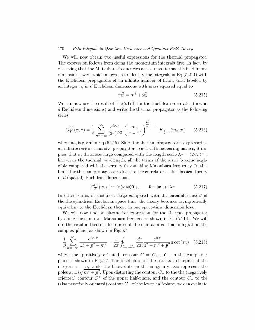
We will now find an alternative expression for the thermal propagatorby doing the sum over Matsubara frequencies shown in Eq.(5.214). We willuse the residue theorem to represent the sum as a contour integral on thecomplex plane, as shown in Fig.5.7
1
β
∞∑
n=−∞
eiωnτ
ω2n + p2 +m2
=1
2π
∮
C+∪C−
dz
2πi
eizτ
z2 +m2 + p2π cot(πz) (5.218)
where the (positively oriented) contour C = C+ ∪ C− in the complex zplane is shown in Fig.5.7. The black dots on the real axis of represent theintegers z = n, while the black dots on the imaginary axis represent thepoles at ±i
√m2 + p2. Upon distorting the contour C+ to the the (negatively
oriented) contour C+ of the upper half-plane, and the contour C− to the(also negatively oriented) contour C− of the lower half-plane, we can evaluate
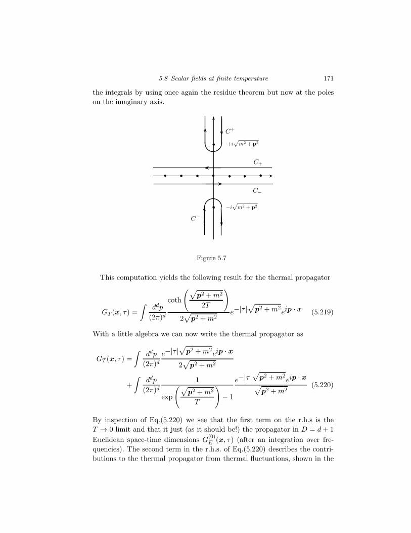
5.8 Scalar fields at finite temperature 171
the integrals by using once again the residue theorem but now at the poleson the imaginary axis.
C+
C−
+i
!
m2 + p2
−i
!
m2 + p2
C+
C−
Figure 5.7
This computation yields the following result for the thermal propagator
GT (x, τ) =
∫ddp
(2π)d
coth
(√p2 +m2
2T
)
2√
p2 +m2e−|τ |
√p2 +m2
eip · x (5.219)
With a little algebra we can now write the thermal propagator as
GT (x, τ) =
∫ddp
(2π)de−|τ |
√p2 +m2
eip · x
2√
p2 +m2
+
∫ddp
(2π)d1
exp
(√p2 +m2
T
)− 1
e−|τ |√
p2 +m2eip · x
√p2 +m2
(5.220)
By inspection of Eq.(5.220) we see that the first term on the r.h.s is theT → 0 limit and that it just (as it should be!) the propagator in D = d+ 1
Euclidean space-time dimensions G(0)E (x, τ) (after an integration over fre-
quencies). The second term in the r.h.s. of Eq.(5.220) describes the contri-butions to the thermal propagator from thermal fluctuations, shown in the

172 Path Integrals in Quantum Mechanics and Quantum Field Theory
form of the Bose occupation numbers (the ‘Bose factor’)
n(p, T ) =1
exp
(√p2 +m2
T
)− 1
(5.221)
Finally, we can find the time-ordered propagator (in real time x0) at finitetemperature T , that we will denote by G(0)(x, x0;T ), by means of the ana-lytic continuation τ → ix0 of the of the thermal propagator of Eq.(5.220).We find,
G(0)(x, x0;T ) = G(0)M (x)
+
∫ddp
(2π)d1
exp
(√p2 +m2
T
)
− 1
e−i|x0|√
p2 +m2eip · x
√p2 +m2
(5.222)
where G(0)M (x) is the (Lorentz-invariant) Minkowski space-time propagator
in D dimensions, given in Section 5.6.4. Notice that the finite temperaturecontribution is not Lorentz invariant.
Related Documents