Passivity Enforcement for Descriptor Systems Via Matrix Pencil Perturbation

532 IEEE TRANSACTIONS ON COMPUTER-AIDED DESIGN OF INTEGRATED CIRCUITS AND SYSTEMS, VOL. 31, NO. 4, APRIL 2012

Passivity Enforcement for Descriptor Systems ViaMatrix Pencil Perturbation

Yuanzhe Wang, Zheng Zhang, Cheng-Kok Koh, Senior Member, IEEE, Guoyong Shi, Senior Member, IEEE,Grantham K. H. Pang, Senior Member, IEEE, and Ngai Wong, Member, IEEE

Abstract—Passivity is an important property of circuits andsystems to guarantee stable global simulation. Nonetheless, non-passive models may result from passive underlying structures dueto numerical or measurement error/inaccuracy. A postprocessingpassivity enforcement algorithm is therefore desirable to perturbthe model to be passive under a controlled error. However, previ-ous literature only reports such passivity enforcement algorithmsfor pole-residue models and regular systems (RSs). In this paper,passivity enforcement algorithms for descriptor systems (DSs, asuperset of RSs) with possibly singular direct term (specifically,D+DT or I−DDT ) are proposed. The proposed algorithms coverall kinds of state-space models (RSs or DSs, with direct termsbeing singular or nonsingular, in the immittance or scatteringrepresentation) and thus have a much wider application scopethan existing algorithms. The passivity enforcement is reduced totwo standard optimization problems that can be solved efficiently.The objective functions in both optimization problems are theerror functions, hence perturbed models with adequate accuracycan be obtained. Numerical examples then verify the efficiencyand robustness of the proposed algorithms.

Index Terms—Descriptor system, immittance representation,passivity enforcement, regular system, scattering representation,symmetric systems.

I. Introduction

PASSIVITY is a crucial property of circuits and systems[1]–[19]; a circuit or system is regarded as passive

(strictly passive) if it does not generate energy (always con-sumes energy). Passivity is an input-output property of asystem and is independent of the internal structure. A lineartime-invariant (LTI) system is passive if and only if its transferfunction is positive real (for immittance representation, i.e., ad-mittance/impedance representation) or bounded real (for scat-

Manuscript received March 7, 2011; revised August 22, 2011; acceptedOctober 18, 2011. Date of current version March 21, 2012. This work wassupported in part by the Hong Kong Research Grants Council, under theGeneral Research Fund 718509E. This paper was recommended by AssociateEditor J. R. Phillips.

Y. Wang is with the Department of Electrical and Computer Engi-neering, Carnegie Mellon University, Pittsburgh, PA 15213 USA (e-mail:[email protected]).

Z. Zhang, G. K. H. Pang, and N. Wong are with the Department ofElectrical and Electronic Engineering, University of Hong Kong, Pokfu-lam 999077, Hong Kong (e-mail: [email protected]; [email protected];[email protected]).

C.-K. Koh is with the School of Electrical and Computer Engi-neering, Purdue University, West Lafayette, IN 47907 USA (e-mail:[email protected]).

G. Shi is with the School of Microelectronics, Shanghai Jiaotong University,Shanghai 201101, China (e-mail: [email protected]).

Color versions of one or more of the figures in this paper are availableonline at http://ieeexplore.ieee.org.

Digital Object Identifier 10.1109/TCAD.2011.2174638

tering representation). A system generated by interconnectingdifferent passive systems is still passive. In contrary, stable butnonpassive systems, when interfaced to other stable systems,may generate an unstable global system [1]. Therefore, toguarantee stable global simulation, we always want to generatepassive models for passive structures such as interconnects,power/ground networks, and others [20]–[22].

In spite of the importance of preserving passivity, non-passive models may be generated from passive underlyingstructures due to numerical/measurement errors. In the contextof data-fitting macromodeling, nonpassivity of macromodelsmay occur due to inappropriate sampling, data noise, fittingerror, etc. [23]–[26]. For example, the macromodels gener-ated using Loewner matrix-based interpolation algorithm arenot guaranteed passive [25]. In the context of model orderreduction, nonpassive reduced-order models may be producedeven though the original full-order models are passive. Thewidely used PRIMA algorithm [27] can only preserve pas-sivity for definite original models, which constitute only asmall subclass of passive models. The positive-real balancedtruncation algorithm is not efficient for very large originalmodels as it has an O(n3

ori) complexity [28]. Note that nori isthe order of the original model (instead of the reduced model),which is usually large. In the context of electromagneticmodeling, nonpassivity may be introduced by discretization,modeling inaccuracy or numerical errors. For instance, thepartial element equivalent circuit (PEEC) models of passiveinterconnect structures may be nonpassive [29], [30]. In allthese instances, the nonpassivity is generally mild, as a soundmodeling algorithm should be precise to certain degrees andcapture the main characteristics of the underlying system.

As a result, postprocessing passivity enforcement algorithmis often desired. Many existing passivity enforcement algo-rithms are developed for pole-residue models, which arisenaturally from vector fitting, by perturbing the residues (orpoles) [13], [31]. Some other algorithms enforce passivity forstate-space models based on Hamiltonian matrix perturbation[7], [8]. However, their application scope is restricted to reg-ular systems (RSs) with nonsingular direct term (specifically,D+DT for immittance representation or I−DDT for scatteringrepresentation). In practice, the direct term can be singular oreven zero in many cases. For instance, the modified nodal anal-ysis models of RCL circuits and the macromodels generated byLoewner matrix-based interpolation are DSs with zero directterms [25], [26], [32]. An extended Hamiltonian matrix pencil

0278-0070/$31.00 c© 2012 IEEE

WANG et al.: PASSIVITY ENFORCEMENT FOR DESCRIPTOR SYSTEMS 533

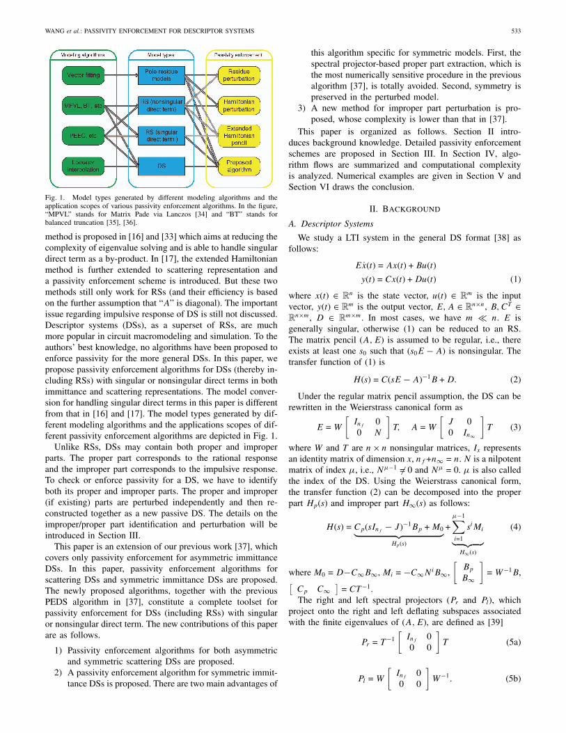
Fig. 1. Model types generated by different modeling algorithms and theapplication scopes of various passivity enforcement algorithms. In the figure,“MPVL” stands for Matrix Pade via Lanczos [34] and “BT” stands forbalanced truncation [35], [36].

method is proposed in [16] and [33] which aims at reducing thecomplexity of eigenvalue solving and is able to handle singulardirect term as a by-product. In [17], the extended Hamiltonianmethod is further extended to scattering representation anda passivity enforcement scheme is introduced. But these twomethods still only work for RSs (and their efficiency is basedon the further assumption that “A” is diagonal). The importantissue regarding impulsive response of DS is still not discussed.Descriptor systems (DSs), as a superset of RSs, are muchmore popular in circuit macromodeling and simulation. To theauthors’ best knowledge, no algorithms have been proposed toenforce passivity for the more general DSs. In this paper, wepropose passivity enforcement algorithms for DSs (thereby in-cluding RSs) with singular or nonsingular direct terms in bothimmittance and scattering representations. The model conver-sion for handling singular direct terms in this paper is differentfrom that in [16] and [17]. The model types generated by dif-ferent modeling algorithms and the applications scopes of dif-ferent passivity enforcement algorithms are depicted in Fig. 1.

Unlike RSs, DSs may contain both proper and improperparts. The proper part corresponds to the rational responseand the improper part corresponds to the impulsive response.To check or enforce passivity for a DS, we have to identifyboth its proper and improper parts. The proper and improper(if existing) parts are perturbed independently and then re-constructed together as a new passive DS. The details on theimproper/proper part identification and perturbation will beintroduced in Section III.

This paper is an extension of our previous work [37], whichcovers only passivity enforcement for asymmetric immittanceDSs. In this paper, passivity enforcement algorithms forscattering DSs and symmetric immittance DSs are proposed.The newly proposed algorithms, together with the previousPEDS algorithm in [37], constitute a complete toolset forpassivity enforcement for DSs (including RSs) with singularor nonsingular direct term. The new contributions of this paperare as follows.

1) Passivity enforcement algorithms for both asymmetricand symmetric scattering DSs are proposed.

2) A passivity enforcement algorithm for symmetric immit-tance DSs is proposed. There are two main advantages of

this algorithm specific for symmetric models. First, thespectral projector-based proper part extraction, which isthe most numerically sensitive procedure in the previousalgorithm [37], is totally avoided. Second, symmetry ispreserved in the perturbed model.

3) A new method for improper part perturbation is pro-posed, whose complexity is lower than that in [37].

This paper is organized as follows. Section II intro-duces background knowledge. Detailed passivity enforcementschemes are proposed in Section III. In Section IV, algo-rithm flows are summarized and computational complexityis analyzed. Numerical examples are given in Section V andSection VI draws the conclusion.

II. Background

A. Descriptor Systems

We study a LTI system in the general DS format [38] asfollows:

Ex(t) = Ax(t) + Bu(t)

y(t) = Cx(t) + Du(t) (1)

where x(t) ∈ Rn is the state vector, u(t) ∈ Rm is the inputvector, y(t) ∈ Rm is the output vector, E, A ∈ Rn×n, B, CT ∈R

n×m, D ∈ Rm×m. In most cases, we have m � n. E isgenerally singular, otherwise (1) can be reduced to an RS.The matrix pencil (A, E) is assumed to be regular, i.e., thereexists at least one s0 such that (s0E − A) is nonsingular. Thetransfer function of (1) is

H(s) = C(sE − A)−1B + D. (2)

Under the regular matrix pencil assumption, the DS can berewritten in the Weierstrass canonical form as

E = W

[Inf

00 N

]T, A = W

[J 00 In∞

]T (3)

where W and T are n × n nonsingular matrices, Ix representsan identity matrix of dimension x, nf +n∞ = n. N is a nilpotentmatrix of index μ, i.e., Nμ−1 �= 0 and Nμ = 0. μ is also calledthe index of the DS. Using the Weierstrass canonical form,the transfer function (2) can be decomposed into the properpart Hp(s) and improper part H∞(s) as follows:

H(s) = Cp(sInf− J)−1Bp + M0︸︷︷︸

Hp(s)

+μ−1∑i=1

siMi︸︷︷︸H∞(s)

(4)

where M0 = D−C∞B∞, Mi = −C∞NiB∞,

[Bp

B∞

]= W−1B,[

Cp C∞]

= CT −1.The right and left spectral projectors (Pr and Pl), which

project onto the right and left deflating subspaces associatedwith the finite eigenvalues of (A, E), are defined as [39]

Pr = T −1

[Inf

00 0

]T (5a)

Pl = W

[Inf

00 0

]W−1. (5b)


It can be readily verified that the transfer function of theprojected DS, namely, (EPr, A, B, C, D) or (PlE, A, B, C, D),is identical to the proper part of the transfer function of theoriginal DS.

B. Symmetric Systems

In this paper, we use ◦ to represent complex conjugate, ◦T

to represent transpose and ◦∗ to represent (complex) conjugatetranspose. The DS in (1) is symmetric if its transfer function(2) satisfies

H(s) = HT (s) (6)

for all s ∈ C that is not a pole of (1). If the transfer functionis written in the decomposed form as (4), the symmetry canbe equivalently defined as

Mi = MTi and CpJjBp = (CpJjBp)T (7)

for all integers i, j ≥ 0. If the proper part (J, Bp, Cp, M0) isboth symmetric and minimal, (J, Bp, Cp) and (JT , CT

p , BTp ) are

similar, i.e., there exists a symmetric and nonsingular matrixT = T T ∈ Rn×n such that [40]

JT = T −1JT, CTp = T −1Bp and BT

p = CpT. (8)

Specifically, if (1) is an single-input-single-output (SISO)system, it is automatically symmetric. A large group of linearnetworks, which are commonly used in package and intercon-nect modelings, have symmetric immittance or scattering ma-trices due to reciprocity. Many algorithms (including balancedtruncation algorithms, passivity characterization algorithms,and others) specifically for symmetric systems have beenproposed in literature [40]–[48]. Passivity enforcement forsymmetric RSs has been handled in [19].

C. Perturbation of Generalized Eigenvalues

For a matrix pencil (M, N) (M, N ∈ Rn×n), if there exist ascalar λ ∈ C and two vectors x, y ∈ Cn that satisfy

Mx = λNx; y∗M = λy∗N (9)

then λ is called the generalized eigenvalue of (M, N) and x, y

are called the right and left eigenvectors associated with λ.The generalized eigenvalue λ can be written as a tuple 〈α, β〉with λ = α/β. If β = 0, λ is an infinite eigenvalue. If the matrixpencil is perturbed by a small matrix pencil (�M, �N), thetuple changes from 〈α, β〉 = 〈y∗Mx, y∗Nx〉 to

⟨α′, β′⟩ = 〈α, β〉 +

⟨y∗�Mx, y∗�Nx

⟩+ O(ε2). (10)

Here ε = ‖[�M �N]‖2, x, y are normalized eigenvectorsassociated with the generalized eigenvalue 〈α, β〉.

D. Hamiltonian and Symplectic Matrices

A real 2n × 2n matrix X is called a Hamiltonian matrix ifit satisfies

J−10 XJ0 = −XT (11)

where J0 =

[0 In

−In 0

]satisfies JT

0 = J−10 = −J0. On the

contrary, X ∈ R2n×2n is called a symplectic matrix if

J−10 XJ0 = XT . (12)

If J is Hamiltonian and K is symplectic, the generalizedeigenvalues λs of (J ,K) distribute symmetrically on the com-plex plane with reference to (w.r.t.) both real and imaginaryaxes. Besides, some matrix X has the following property:

K0XK0 = XT (13)

where K0 =

[0 I

I 0

]= KT

0 = K−10 . This property is named

K0 − property in this paper.

E. Passivity Conditions of a DS

In circuit simulation, an LTI circuit or network can betreated as a black box and fully described by its characteristicparameters. Among the various parameters, admittance param-eter (Y), impedance parameter (Z), and scattering parameter(S) are most commonly used. For a state-space model in theimmittance (Y or Z) representation, it is passive if and only ifits transfer function is positive real. For a state-space modelin the scattering (S) representation, it is passive if and only ifits transfer function is bounded real.

The positive realness of a transfer function H(s) is equiva-lent to:

1) H(s) has no poles with positive real parts;2) G(jω) = 1

2 (H(jω) + H∗(jω)) ≥ 0 for any jω that is nota pole of H(s), ω ∈ R;

3) if jω or ∞ is a pole of H(s), then it is a simple poleand the relevant residue matrix is positive semidefinite.

We use σmax(X) to represent the maximum singular valueof the matrix X. The bounded realness of a transfer functionH(s) is equivalent to:

1) H(s) has no poles with positive real parts;2) sup

ω∈R{σmax(H(jω))} ≤ 1.

For a transfer function written in its decomposed form as(4), it is positive real if and only if:

1) the proper part Hp(s) is positive real;2) the improper part satisfies M1 ≥ 0 and Mi = 0 for i ≥ 2.

It is bounded real if and only if:

1) the proper part Hp(s) is bounded real;2) the improper part is zero, i.e., Mi = 0 for i ≥ 1.

Denote Mν−1 as the highest order moment that is not zero(i.e., Mν−1 �= 0 and Mν = 0). If the DS is in its minimalrealization (i.e., the DS is both controllable and observable),ν = μ. Otherwise, ν ≤ μ [6].

F. GHM Theorems

In this section, we introduced four generalized Hamiltonianmethod (GHM) theorems that relate the positive realness orbounded realness of a DS transfer function to the purelyimaginary or negative real generalized eigenvalues of a ma-trix pencil. These theorems serve as guidelines to pinpoint


passivity violation bands. They also provide information forpassivity enforcement afterward.

Theorem 1: GHM [6]: For a stable, impulse-free DS in theimmittance representation, if 0 is not an eigenvalue of D+DT

2 ,then 0 is an eigenvalue of G(jω) = 1

2 (H(jω) + H∗(jω)) if andonly if jω is a generalized eigenvalue of the matrix pencil(J ,K), where

J =

[A + BQ−1C BQ−1BT

−CT Q−1C −AT − CT Q−1BT

]K =

[E

ET

], Q = −(D + DT ). (14)

Theorem 2: HGHM [47]: For a stable symmetric DS inthe immittance representation with ν = 1 or 2, if 0 is notan eigenvalue of D, then 0 is an eigenvalue of G(jω) =12 (H(jω) + H∗(jω)) if and only if −ω2 is a generalizedeigenvalue of (J ,K), where

J = A − BD−1C, K = EA−1E. (15)

Theorem 3: S-GHM [48]: For a stable impulse-free DS inthe scattering representation, if 1 /∈ σ(D), then 1 ∈ σ(H(jω))if and only if jω is a generalized eigenvalue of (J ,K), with

J =

[A − BDT S−1C −BR−1BT

CT S−1C −AT + CT DR−1BT

]K =

[E

ET

](16)

where S = DDT − I, R = DT D − I, σ(D) represents the setof singular values of D.

Theorem 4: S-HGHM [48]: For a stable symmetric andimpulse-free DS in the scattering representation, if 1 /∈ σ(D),then 1 ∈ σ(H(jω)) if and only if ω2 is a generalized eigenvalueof (J ,K), with

J = A − BDS−1C − BR−1C

K = E(−BR−1C + BDS−1C − A)−1E (17)

where S = DDT − I, R = DT D − I, σ(D) represents the setof singular values of D.

III. Passivity Enforcement Schemes

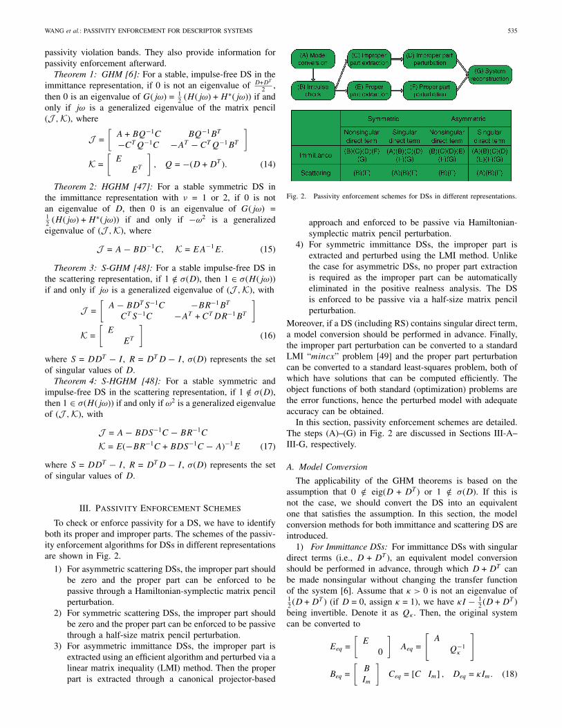
To check or enforce passivity for a DS, we have to identifyboth its proper and improper parts. The schemes of the passiv-ity enforcement algorithms for DSs in different representationsare shown in Fig. 2.

1) For asymmetric scattering DSs, the improper part shouldbe zero and the proper part can be enforced to bepassive through a Hamiltonian-symplectic matrix pencilperturbation.

2) For symmetric scattering DSs, the improper part shouldbe zero and the proper part can be enforced to be passivethrough a half-size matrix pencil perturbation.

3) For asymmetric immittance DSs, the improper part isextracted using an efficient algorithm and perturbed via alinear matrix inequality (LMI) method. Then the properpart is extracted through a canonical projector-based

Fig. 2. Passivity enforcement schemes for DSs in different representations.

approach and enforced to be passive via Hamiltonian-symplectic matrix pencil perturbation.

4) For symmetric immittance DSs, the improper part isextracted and perturbed using the LMI method. Unlikethe case for asymmetric DSs, no proper part extractionis required as the improper part can be automaticallyeliminated in the positive realness analysis. The DSis enforced to be passive via a half-size matrix pencilperturbation.

Moreover, if a DS (including RS) contains singular direct term,a model conversion should be performed in advance. Finally,the improper part perturbation can be converted to a standardLMI “mincx” problem [49] and the proper part perturbationcan be converted to a standard least-squares problem, both ofwhich have solutions that can be computed efficiently. Theobject functions of both standard (optimization) problems arethe error functions, hence the perturbed model with adequateaccuracy can be obtained.

In this section, passivity enforcement schemes are detailed.The steps (A)–(G) in Fig. 2 are discussed in Sections III-A–III-G, respectively.

A. Model Conversion

The applicability of the GHM theorems is based on theassumption that 0 /∈ eig(D + DT ) or 1 /∈ σ(D). If this isnot the case, we should convert the DS into an equivalentone that satisfies the assumption. In this section, the modelconversion methods for both immittance and scattering DS areintroduced.

1) For Immittance DSs: For immittance DSs with singulardirect terms (i.e., D + DT ), an equivalent model conversionshould be performed in advance, through which D + DT canbe made nonsingular without changing the transfer functionof the system [6]. Assume that κ > 0 is not an eigenvalue of12 (D + DT ) (if D = 0, assign κ = 1), we have κI − 1

2 (D + DT )being invertible. Denote it as Qκ. Then, the original systemcan be converted to

Eeq =

[E

0

]Aeq =

[A

Q−1κ

]

Beq =

[B

Im

]Ceq = [C Im] , Deq = κIm. (18)


It can be verified that the model conversion does not changethe transfer function. Besides, it can be proven that an originalRS is converted to an impulse-free DS and an original DS isconverted to a DS with the same index.

2) For Scattering DSs: For scattering DSs with singulardirect terms (i.e., I − DDT ), an equivalent model conversionshould be performed in advance, through which I −DDT canbe made nonsingular without changing the transfer functionof the system [48]. Let 0 < κ < 1, we have

Eeq =

[E

0

]Aeq =

[A

Im

]Beq =

[B

κIm − D

]Ceq = [C Im] , Deq = κIm. (19)

The transfer function of the equivalent model (18) is iden-tical to that of the original model [48]. I −DeqD

Teq = (1−κ2)I

is guaranteed to be nonsingular. If the original model is an RSor an impulse-free DS, the converted model is an impulse-freeDS.

B. Impulse Check

According to Section II-E, the passivity conditions for im-mittance and scattering DSs both involve the existence checkof the improper part (impulsive response). Directly computingthe Weierstrass canonical form (3) of a DS is known tobe prohibitively expensive and ill-conditioned. Therefore, weintroduce a new method to calculate ν. Consider the transferfunction in (4), we calculate the limit (note that the limit � isan m by m matrix and s−1 is a scalar multiplied to the matrixH(s)) as follows:

� = lims→∞ s−1H(s). (20)

1) For immittance DSs:a) if � = 0, ν = 1, the DS is impulse-free;b) if � = ∞, ν > 2, the DS is definitely nonpassive;c) if � = constant �= 0, ν = 2, improper part extrac-

tion and possible proper part extraction should beperformed.

2) For scattering DSs:a) if � = 0, ν = 1, the DS is impulse-free;b) if � = constant �= 0 or � = ∞, ν ≥ 2, the DS is

definitely nonpassive.In practice, � can be calculated by substituting two large

positive number s1, s2 � 0 with s1 = γs2 (3 < γ < 10) . If‖H(s1)‖2‖H(s2)‖2

<< γ , � = 0; if ‖H(s1)‖2‖H(s2)‖2

= γ , � = constant; otherwise,� = ∞. As the DSs discussed are stable, all the poles aredistributed on the left half of complex plane. Thus sE − A isalways invertible when s > 0. The numerical stability and highefficiency of this method has also been verified by real-worldexamples of orders from hundreds to tens of thousands.

C. Improper Part Extraction

If � = constant �= 0 for immittance DSs, improper partshould be extracted and perturbed to be positive semidefinite toguarantee passivity. Improper part extraction can be performedby limit calculation as follows:

M1 = lims→∞ s−1H(s). (21)

Alternatively, the improper part can be calculated usingcanonical projector methods. Right and left spectral projectors(Pr and Pl) can be calculated in three steps [50]–[52]. Thenthe improper is extracted as the transfer function of a new DS(E∞, A, B, C, D) minus H(0), that is

sM1 = C (sE∞ − A)−1 B + D − H(0) (22)

where E∞ = E(I − Pr) or E∞ = (I − Pl)E.In practice, we can substitute an arbitrary positive number

s1 into (21) as follows:

M1 =1

s1

(C (s1E∞ − A)−1 B + D − H(0)

). (23)

It should be noted that improper part extraction only appliesto passivity enforcement of immittance DSs, as shown inFig. 2.

D. Improper Part Perturbation

The improper part, if exists, has been extracted as sM1.To enforce passivity, we should perturb M1 to be positivesemidefinite. The following optimization problem should besolved:

minM1

‖M1 − M1‖∞ subject to M1 ≥ 0. (24)

The optimization problem (24) can be solved using MAT-LAB LMI toolbox by converting it to a standard “mincx”problem [53] as follows:

mine∈R

es.t.

⎧⎪⎪⎨⎪⎪⎩

M1 > 0,

−tij ≤ mij − mij ≤ tij, (1 ≤ i ≤ m, i ≤ j ≤ m)i−1∑j=1

tji + tii +m∑

j=i+1tij ≤ e. (1 ≤ i ≤ m)

(25)where mij (i ≤ j, mji = mij) represents the (i, j)th element ofM1, mij (i ≤ j, mji = mij) represents the (i, j)th element of M1.

Lemma 1: The solution of the optimization problem (25) isidentical to that of (24).

Proof: See Appendix A.Note that the size of M1 is m (i.e., the number of ports,

which is usually small). Hence the computational complexityof solving (25) is low, even lower than the method in [37].sM1 is the perturbed improper part, which, together with theperturbed proper part, can be reconstructed as a new DS (seeSection III-G).

E. Proper Part Extraction

For immittance DSs, if � = constant �= 0 according toimpulse check, proper part should be extracted. However, theproper part extraction can be avoided if the immittance DS issymmetric, as shown in Fig. 2. Therefore, this step only appliesto passivity enforcement of asymmetric immittance DSs.

1) For Symmetric Immittance DSs: For a symmetric im-mittance DS, because M1 = MT

1 [see (7)], we have

H(jω) + H∗(jω) = Hp(jω) + jωM1 + HTp (−jω) − jωMT

1

= Hp(jω) + HTp (−jω). (26)


Hence the improper part sM1 will be automatically canceled inthe subsequent positive realness analysis. Therefore, no properpart extraction is required.

2) For Asymmetric Immittance DSs: For asymmetric DSs,the proper part can be extracted as the transfer function of anew DS (Ep = EPr, A, B, C, D) or (Ep = PlE, A, B, C, D),that is

Hp(s) = C(sEp − A)−1B + D. (27)

The projection matrices Pl and Pr can be computed usingthe canonical projector-based method. The canonical projector-based method is relatively robust and does not require thecomputation of W and T [see (5a) and (5b)]. The readersare referred to [51] and [52] for the details of the canonicalprojector-based method.

F. Proper Part Perturbation

The proper part mentioned in this section is the projectedDS (Ep, A, B, C, D) for asymmetric immittance DS or theoriginal DS (E, A, B, C, D) for scattering DS and symmetricimmittance DS. We do not distinguish between E and Ep

in this section with the implication that E means Ep forasymmetric immittance DSs. For DSs in different represen-tations, we should perturb different matrix pencil to enforcepassivity. However, the error control scheme is the same.In the remainder of this subsection, we will first propose aerror control scheme. Then, we will propose the matrix pencilperturbations for scattering DSs, symmetric immittance DSsand asymmetric immittance DSs, respectively. Symmetry ispreserved in the process of matrix pencil perturbation forsymmetric immittance DSs, which follows that (26) alwaysholds. Thus, proper part extraction is not required. The meth-ods introduced in this section are direct generalizations of theprocedure in [7].

1) Error Control: According to Theorems 1–3, we canenforce passivity by perturbing the matrix pencil (J ,K). Thematrix pencils (J ,K), as defined in (14)–(16), are constructedby state-space matrices E, A, B, C, D. Hence at least oneof the state-space matrices has to be perturbed. Here wechoose to perturb the matrix C for the following reasons.First, E and A should remain unchanged to guarantee thatthe perturbed system remains stable and to preserve thekey dynamic properties of the system (pole distribution).Second, the perturbation of D will introduce inaccuracy inthe whole frequency band. Thus we keep D unperturbed.The only choice is to perturb B and/or C, which is con-venient as the transfer function is a linear function of C

and B. Only C is perturbed in the following discussion forsimplicity.

We derive a criterion to control the error introduced byperturbing C. Assuming the impulse response (inverse Laplacetransform of transfer function) of the DS (E, A, B, C, D)is h(t), the error of the perturbed model can be measuredby

� =∫ ∞

0‖dh(t)‖2

Fdt =∫ ∞

0trace

(dh(t)dhT (t)

)dt. (28)

As dh(t) = dCF(t)B with F(t) = T −1

[eJt 00 0

]W−1, we

have

� = trace(dCGpcdCT

). (29)

Here,

Gpc =∫ ∞

0F(t)BBTFT (t)dt (30)

is called the proper controllability Gramian, which can besolved from the projected generalized Lyapunov equations [39]as follows:

EGpcAT + AGpcE

T = −PlBBT PTl ,

Gpc = PrGpc. (31)

Assume that Gpc = LT L (Cholesky factorization), a coordi-nate transformation is performed as follows:

dCt = dCLT . (32)

Thus,

� = trace(dCtdCT

t

)= ‖dCt‖2

F = ‖vec(dCt)‖22. (33)

Here, vec(X) is a vector constructed by stacking all thecolumns of X.

2) For Asymmetric Scattering DSs: We begin with aneat method (as Proposition 1) to pinpoint the frequencybands where passivity violations occur. Compared with theHamiltonian method for RSs [7], the proposed method doesnot require the relatively expensive calculation of slopes. Forhandling multiple purely imaginary eigenvalues, we refer thereaders to [7] for details.

Proposition 1: Assume that the set = {jωi} (i =1, 2, . . . , k) contains all purely imaginary eigenvalues of(J ,K) with positive imaginary parts, sorted in ascendingorder, which divide the frequency band [0, +∞) into k + 1segments. Calculate σ(H(jω)) at the center frequency of eachsegment (for the (k +1)th segment the frequency is selected as32jωk). If σmax(H(jω)) ≤ 1 for the segment defined by jωi andjωi+1, then the system is passive in this frequency segment,otherwise it is nonpassive.

The above proposition involves identification of the purelyimaginary eigenvalues. In practice, the purely imaginary eigen-values have small real parts introduced by rounding errors. In[7], a bound is selected a priori and eigenvalues with real partsunder this bound are interpreted as “purely imaginary.” But indifferent problems the numerical errors may be very different,which renders it very difficult to choose this bound. A morerobust criterion is proposed here.

Lemma 2: All the generalized eigenvalues of (J ,K)distribute symmetrically w.r.t. both real and imaginaryaxes.

Proof: See Appendix B.Hence, all the complex but not purely imaginary eigenvalues

have mirrors w.r.t. imaginary axis. They appear in the form of±σ ± jω (four in a group). The purely imaginary eigenvaluesdo not have such mirrors w.r.t. the imaginary axis and they


appear in the form of σ ± jω (two in a group). The imple-mentation of imaginary generalized eigenvalues identificationis detailed as follows.

a) Select a loose bound ξ.b) Find all the λi’s with Re(λi) < ξ. These λi’s form a set

1.c) For each λi ∈ 1, check whether there exists a λj (j �= i)

such that |λj − (−λi)| < 2Re(λi). If no such λj exists,λi is determined as imaginary.

Now we move on to discuss matrix pencil perturbation. IfC is perturbed by a small matrix dC, the symplectic matrix Kremains the same while the Hamiltonian matrix J is perturbedby dJ , with

dJ =

[ −BDT S−1dC 0dCT S−1C + CT S−1dC dCT DR−1BT

]dK = 0

(34)where S = DDT −I, R = DT D−I are both symmetric. Similarto J , dJ is readily checked to be Hamiltonian.

As a result, the generalized eigenvalues of (J ,K) changefrom λ to λ′ [see (10)] as follows:

λ′ =α′

β=

α + �α

β= λ +

y∗dJ x

y∗Kx. (35)

Lemma 3: For a purely imaginary generalized eigenvalueof (J ,K), the right and left eigenvectors x, y associated withit satisfy y = J0x.

Proof: See Appendix C.Consequently, (35) can be rewritten as

λ′ − λ =x∗J0dJ x

x∗J0Kx. (36)

As J−10 dJ J0 = −dJ T , J−1

0 KJ0 = KT , we have J0dJ =dJ T JT

0 and J0K = −KT JT0 , i.e., J0dJ is real symmetric and

J0K is real and skew symmetric. It follows that x∗J0dJ x isreal and x∗J0Kx is purely imaginary. As a result, λ′ remainspurely imaginary if λ is purely imaginary.

Let the ith purely imaginary eigenvalue of (J ,K) be jωi

and it is supposed to be moved to jωi. Suppose that σ(H(jω))between jωi and jωi+1 (ωi < ωi+1) exceeds 1, ωi can be chosenas

ωi = ωi + ε(ωi+1 − ωi). (37)

Here, 0 < ε < 0.5. As the selection of ωi is partially heuristic,the perturbed DS should be treated as a new input and gothrough the passivity check procedure again. If nonpassive,iterative perturbations should be performed. In practice, theiteration number is usually no more than 5 if the passivityviolation is mild (which ought to be the case when theunderlying system is intrinsically passive).

Split xi into two vectors of the same size xi =

[xi,1

xi,2

]and

denote zi = S−1(Cxi,1 + DBT xi,2). Using Kronecker productproperty, (36) can be transformed as

Re((

xTi,1L

−1) ⊗ z∗

i

) × vec(dCt) = (ωi − ωi)Im(x∗

i,2Exi,1).

(38)

Here dCt = dCLT is substituted into (38) to facilitate theerror control, as the perturbation error � is the square of theFrobenius norm of dCt . In (38), the perturbation matrix Ct isisolated. Denote

mi = Re((

xTi,1L

−1) ⊗ z∗

i

)(39a)

ni = (ωi − ωi)Im(x∗

i,2Exi,1). (39b)

If there exist k generalized eigenvalues to be moved, (38)can be incorporated k times as a matrix format as

min ‖vec(dCt)‖2, subject to M × vec(dCt) = N (40)

where M =

⎡⎢⎣ m1

...mk

⎤⎥⎦ ∈ Rk×mn, N =

⎡⎢⎣ n1

...nk

⎤⎥⎦ ∈ Rk×1.

This is a standard least-squares problem which can be solvedefficiently. The constraint is an underdetermined equation asthe number of unknowns mn far exceeds the number ofequations k, i.e., k � mn. Two possible ways of solvingthis problem are the pseudoinverse method and the orthogonalmatrix triangularization (QR)-factorization method. For thepseudoinverse method, the solution is MT (MMT )−1N. Forthe QR-factorization method, the solution is MQMR

−T N withMQMR = MT being a QR-factorization of MT . The perturbedpassive proper part is (E, A, B, C, D) with C = C + dCtL

−T .3) For Symmetric Scattering DSs: For symmetric scatter-

ing DSs, symmetry should be preserved in the perturbationprocedures. A symmetric scattering DS (E, A, B, C, D) canbe rewritten as (Es, As, Bs, Cs, Ds), where

Es =

[E

ET

], As =

[A

AT

], Bs =

[B

CT

]Cs =

[1

2C

1

2BT

], Ds =

1

2

(D + DT

). (41)

Note that (41) is not a definition of “symmetry” but anequivalent model conversion. The definition of symmetry isgiven in Section II-B. The transfer function of the DS in (41)reads

Hs(s) =1

2

(C(sE − A)−1B+D+BT (sET −AT )−1CT + DT

)= C(sE − A)−1B + D = H(s). (42)

Besides, the DS (Es, As, Bs, Cs, Ds) remains symmetric nomatter how we perturb the matrix C. Subsequently, the matrixpencil in (17) reads

J =

[A − BXC −BXBT

−CT XC AT − CT XBT

]

K =

[E

ET

] [BYC − A BYBT

CT YC CT YBT − AT

]−1

[E

ET

](43)

whereX = (D + DT − 2I)−1

Y = (D + DT + 2I)−1. (44)

It is readily verified that both J and K have K0-property.


An error bound of the perturbed DS (52) is introducedas follows. Assume that if we perturb matrix C by dC, theperturbation of the impulse response of the original DS isdh(t) and that of the symmetric DS (52) is dhs(t), we have

‖dhs(t)‖F = ‖1

2dh(t) +

1

2dhT (t)‖F

≤ 1

2‖dh(t)‖F +

1

2‖dhT (t)‖F = ‖dh(t)‖F .

Thus ‖dh(t)‖F can be used as an upper bound of ‖dhs(t)‖F .As a result, similar procedures as in Section III-F1 canbe performed to obtain the coordinate transform matrix L,which can be used to control the error of perturbation in thesymmetric case as will be discussed below.

If C is perturbed by a small matrix dC, We have

dJ = −[

BXdC

dCT XC + CT XdC dCT XBT

]dK =

[E

ET

] [K11 K12

K21 K22

]·[

BYdC

dCT YC + CT YdC dCT YBT

][

K11 K12

K21 K22

] [E

ET

](45)

where[K11 K12

K21 K22

]=

[BYC − A BYBT

CT YC CT YBT − AT

]−1

with the property that K11 = KT22 and K12 = KT

12 andK21 = KT

21. dJ and dK are also readily checked to haveK0 − property.

According to (10), we have

λ′ =α′

β′ =α + �α

β + �β= ω2 +

�αβ − α�β

β2

= λ +(y∗dJ x)(y∗Kx) − (y∗J x)(y∗dKx)

(y∗Kx)2. (46)

Lemma 4: For a real eigenvalue λ, the eigenvectors x, y

associated with it satisfy y = K0x.Proof: See Appendix D.

Thus (46) becomes

λ′ = λ+(x∗K0dJ x)(x∗K0Kx) − (x∗K0J x)(x∗K0dKx)

(x∗K0Kx)2. (47)

As K0dJ , K0dK, K0J , and K0K are all symmetric, thenumerator and denominator of (47) are both real. Therefore,if the original eigenvalue λ is real, the perturbed eigenvalueλ′ is still real. Let

k1 =1

x∗K0Kx, k2 =

x∗K0J x

(x∗K0Kx)2(48)

which are both real numbers. Equation (47) can be rewrittenas

ω2i = ω2

i + k1x∗i K0dJ xi − k2x

∗i K0dKxi. (49)

Splitting xi into two vectors of the same dimensions xi1 andxi2, followed by similar calculation as in Section III-F2, wehave an optimization problem similar to (40), with

mi = 2Re(k1(xT

i1L−1) ⊗ z∗

i1

+k2(xTi1E

T K22L−1 + xT

i2EK12L−1) ⊗ (z∗

i2 + z∗i3)

)zi1 = X(Cxi1 + BT xi2), zi2 = Y (BT K21 + CK11)Exi1

zi3 = Y (BT K22 + CK12)ET xi2, ni = ω2i − ω2

i . (50)

With the solution dCt , we have C = C + dCtL−T and the

perturbed DS being

Es =

[E

ET

], As =

[A

AT

], Bs =

[B

CT

]

Cs =

[1

2C

1

2BT

], Ds =

1

2

(D + DT

). (51)

4) For Asymmetric Immittance DSs: For asymmetric im-mittance DSs, proper part perturbation requires solving asimilar least-square problem as (40) with the same defini-tion of mi and ni as in (39a). The only difference is thatzi = (D + DT )−1(Cxi,1 + BT xi,2) in this case. The perturbedpassive proper part is (E, A, B, C, D) with C = C + dCtL

−T .5) For Symmetric Immittance DSs: The deduction in

this subsection is very similar to that in Section III-F3.For symmetric immittance DSs, symmetry should be pre-served in the perturbation procedures to totally avoid thenumerically sensitive proper part extraction. A symmetricimmittance DS (E, A, B, C, D) can be similarly rewritten as(Es, As, Bs, Cs, Ds), where

Es =

[E

ET

], As =

[A

AT

], Bs =

[B

CT

]Cs =

[1

2C

1

2BT

], Ds =

1

2

(D + DT

). (52)

To compute the perturbed DS, we have to solve an opti-mization problem similar to (40), with

mi = Re((xT

i1L−1) ⊗ z∗

i

)(53a)

ni = (ω2i − ω2

i )Re(x∗2EA−1Ex1) (53b)

zi = Q−10 (Cxi1 + BT xi2). (53c)

With the solution dCt , we have C = C + dCtL−T and the

perturbed DS being

Esp =

[E

ET

], Asp =

[A

AT

], Bsp =

[B

CT

]

Csp =

[1

2C

1

2BT

], Ds =

1

2

(D + DT

). (54)

This perturbed DS can pass the passivity check in Theo-rem 2, but may contain nonpassive improper part. To ensurethe passivity of the improper part, a system recovery shouldbe performed as discussed in Section III-G.

G. System Reconstruction

System reconstruction only applies to immittance DSs whenimproper part exists. The perturbed improper and proper partsare reconstructed as a new DS for further use.


1) For Asymmetric Immittance DS: For an asymmetricimmittance DS, the reconstructed DS reads

E′ =

⎡⎣ Ep

0 Im

0 0

⎤⎦ A′ =

⎡⎣ Ap

Im

Im

⎤⎦

B′ =

⎡⎣ B

0LT

⎤⎦ C′ =

[C − L 0

]D′ = D (55)

where M1 = LT L is the Cholesky factorization of M1. One caneasily check that the transfer function of this DS is identical tothe sum of the proper and improper parts. Besides, A′ remainsnonsingular if A is nonsingular and E′ is index-2 if E is index-

2 (note that the matrix block

[0 Im

0 0

]is index-2).

2) For Symmetric Immittance DS: For a symmetric immit-tance DS, the reconstructed DS reads

E′ =

⎡⎣ Esp

0 Im

0 0

⎤⎦ A′ =

⎡⎣ Asp

Im

Im

⎤⎦

B′ =

⎡⎣ Bsp

0M1 − M

(p)1

⎤⎦ C′ =

[Csp − Im 0

], D′ = Dsp. (56)

Here, M(p)1 is the improper part obtained by performing the

improper part extraction again on the perturbed symmetric DS(54). One can easily check that the transfer function of this DSequals to the sum of the perturbed passive proper and improperparts. Consequently, the transfer function is still symmetric.

IV. Algorithm Flow and Complexity Analysis

A. For Asymmetric Scattering DS

1) Step A (model conversion): This step is merely areformulation of the matrices and its computation isnegligible.

2) Step B (impulse check): This step involves matrix-vectoroperation and has low computational complexity. SparseLU-decomposition can be utilized if the DS is sparse.

3) Step F (proper part perturbation):

a) Calculation of coordinate transform matrix L:This procedure requires solving the projected gen-eralized Lyapunov equations (31) and its Choleskydecomposition. The computational complexity isO(n3).

b) Iterative matrix pencil perturbation: This pro-cedure dominates the computation time of thealgorithm. In each iteration, a generalized eigen-value problem and a least-squares optimizationproblem should be solved. The complexity of thegeneralized eigenvalue problem is O((2n)3), withn being the order of the model. The least-squaresoptimization problem requires O(nmk2), with m

being the number of ports and k being the numberof eigenvalues to be perturbed. In most cases wehave m � n and k � n. The iteration numberusually does not exceed 5.

Fig. 3. (First example.) We perturb the original model to be passive.(a) Eigenvalue plot of G(jω). (b) Generalized eigenvalue distribution of thematrix pencil (J ,K).

In summary, the complexity of the algorithm is O(n3 × iter)and is dominated by the iterative matrix pencil perturbationprocedure.

B. For Symmetric Scattering DS

1) Steps A–B: Same as the analysis in Section IV-A.2) Step F (proper part perturbation):

a) Calculation of coordinate transform matrix L:This procedure requires solving the same pro-jected generalized Lyapunov equations as in theasymmetric scattering DS case. The computationalcomplexity is O(n3).

b) Iterative matrix pencil perturbation: The dimen-sion of the half-size matrix pencil is also 2n dueto the model conversion in (41). Hence, the com-plexity is the same as the analysis in Section IV-A.

In summary, the complexity of the algorithm is O(n3×iter).

C. For Symmetric Immittance DS

1) Steps A–B: Same as the analysis in Section IV-A.2) Step C (improper part extraction): Improper part extrac-

tion can be done in the process of impulse check. Thusno additional calculation is needed for this step.

3) Step D (improper part perturbation): This step involvessolving an LMI “mincx” problem, with one dimension-m constraint and m(m + 3)/2 dimension-1 constraints.m is the number of ports which is usually small. Thecomputational complexity of this procedure is low.

4) Step F: Same as the analysis in Section IV-A.


Fig. 4. (First example.) We perturb the original model to be “more” non-passive. (a) Eigenvalue plot of G(jω). (b) Generalized eigenvalue distributionof the matrix pencil (J ,K).

5) Step G (system reconstruction): This step is merely areformulation of the matrices and its computation isnegligible.


D. For Asymmetric Immittance DS

1) Steps A–D: Same as the analysis in Section IV-C.2) Step E (proper part extraction): This step involves

canonical projector computation. The complexity isO(n3).

3) Steps F–G: Same as the analysis in Section IV-C.


E. Summary of Complexity Analysis

The algorithm flows for asymmetric and symmetric scat-tering DSs both involve three steps: model conversion(Step A), impulse check (Step B), and proper part perturbation(Step F). The algorithm flow for symmetric immittance DSsinvolves three more steps: improper part extraction (Step C),improper part extraction (Step D), and system reconstruction(Step G). The algorithm flow for asymmetric immittance DSsrequires one more step than that for symmetric immittanceDSs: proper part extraction (Step E).

Among Steps A–G, the proper part perturbation (Step F)has the largest complexity. As the algorithm flows for all thefour types of DSs involve Step F, the overall complexities forall the four algorithm flows are O(n3 × iter).

Fig. 5. (Second example.) Singular value patterns of H(jω) of the(a) original nonpassive model and the (b) perturbed passive model.

V. Numerical Examples

A. PEEC Reduced-Order Model

The model used in this example is a PEEC reduced-ordermodel [54]. The original model is an SISO DS of order 480,with D = 0. A reduced-order model (with the order being35) is obtained using PRIMA. The model is in the immittancerepresentation and is nonpassive at the frequency band froms1 = 1.15j (rad/s) to s2 = 1.39j (rad/s). To enforce passivity,we perturb s1 to higher frequency and s2 to lower frequency,with the displacement being 0.28 ∗ |s2 − s1|. The eigenvalueplots of G(jω) of the original and perturbed models are shownin Fig. 3(a), from which we conclude that the perturbed modelis passive. The original, first-order approximated and realperturbed s1, s2 are shown in Fig. 3(b). It can be seen thatalthough the first-order approximations of s1, s2 remain onthe imaginary axis, the real perturbed s1, s2 are moved offthe imaginary axis. On the other hand, if we perturb s1, s2

wrongly with the same amount but in the other directions,the perturbed s1, s2 remain on the imaginary axis and theperturbed model is nonpassive (in fact “more” nonpassive),as shown in Fig. 4. We use this wrong perturbation result toillustrate how the purely imaginary eigenvalues move on thecomplex plane. In practice, we should of course choose theright perturbation direction according to the criterion proposedin Section III-F.


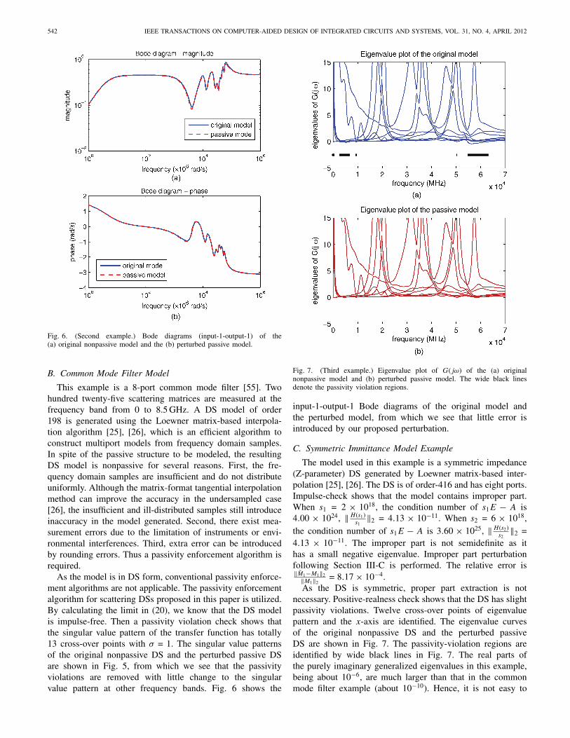
Fig. 6. (Second example.) Bode diagrams (input-1-output-1) of the(a) original nonpassive model and the (b) perturbed passive model.

B. Common Mode Filter Model

This example is a 8-port common mode filter [55]. Twohundred twenty-five scattering matrices are measured at thefrequency band from 0 to 8.5 GHz. A DS model of order198 is generated using the Loewner matrix-based interpola-tion algorithm [25], [26], which is an efficient algorithm toconstruct multiport models from frequency domain samples.In spite of the passive structure to be modeled, the resultingDS model is nonpassive for several reasons. First, the fre-quency domain samples are insufficient and do not distributeuniformly. Although the matrix-format tangential interpolationmethod can improve the accuracy in the undersampled case[26], the insufficient and ill-distributed samples still introduceinaccuracy in the model generated. Second, there exist mea-surement errors due to the limitation of instruments or envi-ronmental interferences. Third, extra error can be introducedby rounding errors. Thus a passivity enforcement algorithm isrequired.

As the model is in DS form, conventional passivity enforce-ment algorithms are not applicable. The passivity enforcementalgorithm for scattering DSs proposed in this paper is utilized.By calculating the limit in (20), we know that the DS modelis impulse-free. Then a passivity violation check shows thatthe singular value pattern of the transfer function has totally13 cross-over points with σ = 1. The singular value patternsof the original nonpassive DS and the perturbed passive DSare shown in Fig. 5, from which we see that the passivityviolations are removed with little change to the singularvalue pattern at other frequency bands. Fig. 6 shows the

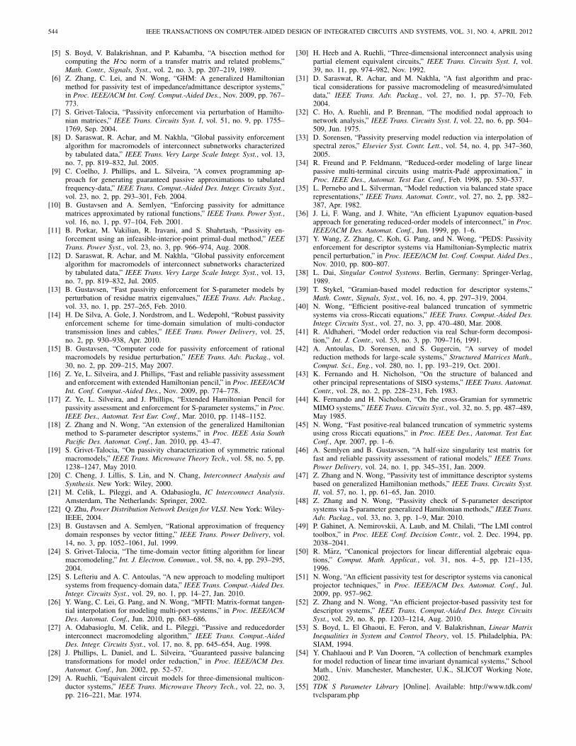
Fig. 7. (Third example.) Eigenvalue plot of G(jω) of the (a) originalnonpassive model and (b) perturbed passive model. The wide black linesdenote the passivity violation regions.

input-1-output-1 Bode diagrams of the original model andthe perturbed model, from which we see that little error isintroduced by our proposed perturbation.

C. Symmetric Immittance Model Example

The model used in this example is a symmetric impedance(Z-parameter) DS generated by Loewner matrix-based inter-polation [25], [26]. The DS is of order-416 and has eight ports.Impulse-check shows that the model contains improper part.When s1 = 2 × 1018, the condition number of s1E − A is4.00 × 1024, ‖H(s1)

s1‖2 = 4.13 × 10−11. When s2 = 6 × 1018,

the condition number of s1E − A is 3.60 × 1025, ‖H(s2)s2

‖2 =4.13 × 10−11. The improper part is not semidefinite as ithas a small negative eigenvalue. Improper part perturbationfollowing Section III-C is performed. The relative error is‖M1−M1‖2

‖M1‖2= 8.17 × 10−4.

As the DS is symmetric, proper part extraction is notnecessary. Positive-realness check shows that the DS has slightpassivity violations. Twelve cross-over points of eigenvaluepattern and the x-axis are identified. The eigenvalue curvesof the original nonpassive DS and the perturbed passiveDS are shown in Fig. 7. The passivity-violation regions areidentified by wide black lines in Fig. 7. The real parts ofthe purely imaginary generalized eigenvalues in this example,being about 10−6, are much larger than that in the commonmode filter example (about 10−10). Hence, it is not easy to


Fig. 8. (Third example.) Bode diagrams (input-1-output-1) of the (a) originalnonpassive model and (b) perturbed passive model.

set a bound a priori to determine which eigenvalue should beidentified as “purely imaginary.” Therefore, the more reliablecriterion in Section III-F2 can be used.

Bode diagrams of the original model and the passive model(input-1-output-1) are shown in Fig. 8, from which we con-clude that the error introduced by perturbation is small. Itcan be seen from the Bode diagram that the improper partis dominant at the high frequency region.

Alternatively, we also employ the algorithm in [37] bytreating the DS as asymmetric. Proper part extraction isthereby performed. We use the following metric to mea-sure the overall error introduced by different perturba-tions:

Err =1

k

∑s=s1,...,sk

‖H(s) − H(s)‖2

‖H(s)‖2(57)

where H(s) is the transfer function of the original model andH(s) is that of the perturbed model, s1, . . . , sk are frequenciesof the samples we use to generate the model. It turns out thatErr = 7.16 × 10−3 if we employ the algorithm for symmetricimmittance DS and Err = 2.02×10−2 if proper part extractionis performed. On the other hand, the CPU time is 4.6 × 10−3

sec which is larger than that if the algorithm for symmetricimmittance DSs is employed (3.8 × 10−3 s). We conclude thatavoidance of proper part extraction is favorable for betterperturbation accuracy.

VI. Conclusion

This paper has generalized the results in [37] and is thefirst work reported in the literature to enforce passivity forDSs. Following a possible system decomposition, the improperpart perturbation was converted into a standard LMI “mincx”problem and the proper part perturbation into a standard least-squares problem, both of which can be solved efficiently undercontrolled perturbation errors. Numerical examples have veri-fied the efficiency and accuracy of the proposed algorithms.

appendix A

Proof of Lemma 1

It is straightforward to prove that e ≥ max1≤i≤m

m∑j=1

|mij − mij|,which indicates that e ≥ ‖M1 − M1‖∞.

appendix B

Proof of Lemma 2

It is obvious that if J ,K are real, the eigenvalues are inconjugate pairs. On the other hand, if λ is a generalized eigen-value of (J ,K), J x = λKx, xTJ T = λxTKT , −xT J−1

0 J J0 =λxT J−1

0 KJ0. Assume y∗ = xT J−10 , we have y∗J = −λy∗K,

which means −λ is also an eigenvalue of (J ,K). So every λ

implies coexistence of the tuple (λ, λ, −λ, −λ).

appendix C

Proof of Lemma 3

x is the right eigenvector of (J ,K) indicates J x = λKx.Performing conjugate transpose on both sides, and noting thatλ is imaginary and J , K are real, we have x∗J T = −λx∗KT .Because J is Hamiltonian and K is symplectic, we havex∗(−J−1

0 J J0) = −λx∗(J−10 KJ0). Hence x∗J−1

0 J = λx∗J−10 K.

According to the definition of left eigenvector, x∗J−10 is

equivalent to y∗, i.e., y = J0x.

appendix D

Proof of Lemma 4

Perform conjugate transpose on both sides of J x = λKx,we have x∗J T = λx∗KT (note that λ is real). As J and K bothhave K0 −property, x∗K0JK0 = λx∗K0KK0, i.e., (x∗K0)J =λ(x∗K0)K. According to the definition of left eigenvector (9),we have y∗ = x∗K0, i.e., y = K0x.

References

[1] E. Kuh and R. Rohrer, Theory of Linear Active Networks. San Francisco,CA: Holden-Day, 1967.

[2] R. Freund and F. Jarre, “An extension of the positive real lemma todescriptor systems,” Optimiz. Methods Softw., vol. 19, no. 1, pp. 69–87,2004.

[3] L. Zhang, J. Lam, and S. Xu, “On positive realness of descriptorsystems,” IEEE Trans. Circuits Syst. I, vol. 49, no. 3, pp. 401–407,Mar. 2002.

[4] Y. Liu and N. Wong, “Fast sweeping methods for checking passivityof descriptor systems,” in Proc. IEEE Asia Pacific Conf. Circuits Syst.,Nov.–Dec. 2008, pp. 1794–1797.


[5] S. Boyd, V. Balakrishnan, and P. Kabamba, “A bisection method forcomputing the H∞ norm of a transfer matrix and related problems,”Math. Contr., Signals, Syst., vol. 2, no. 3, pp. 207–219, 1989.

[6] Z. Zhang, C. Lei, and N. Wong, “GHM: A generalized Hamiltonianmethod for passivity test of impedance/admittance descriptor systems,”in Proc. IEEE/ACM Int. Conf. Comput.-Aided Des., Nov. 2009, pp. 767–773.

[7] S. Grivet-Talocia, “Passivity enforcement via perturbation of Hamilto-nian matrices,” IEEE Trans. Circuits Syst. I, vol. 51, no. 9, pp. 1755–1769, Sep. 2004.

[8] D. Saraswat, R. Achar, and M. Nakhla, “Global passivity enforcementalgorithm for macromodels of interconnect subnetworks characterizedby tabulated data,” IEEE Trans. Very Large Scale Integr. Syst., vol. 13,no. 7, pp. 819–832, Jul. 2005.

[9] C. Coelho, J. Phillips, and L. Silveira, “A convex programming ap-proach for generating guaranteed passive approximations to tabulatedfrequency-data,” IEEE Trans. Comput.-Aided Des. Integr. Circuits Syst.,vol. 23, no. 2, pp. 293–301, Feb. 2004.

[10] B. Gustavsen and A. Semlyen, “Enforcing passivity for admittancematrices approximated by rational functions,” IEEE Trans. Power Syst.,vol. 16, no. 1, pp. 97–104, Feb. 2001.

[11] B. Porkar, M. Vakilian, R. Iravani, and S. Shahrtash, “Passivity en-forcement using an infeasible-interior-point primal-dual method,” IEEETrans. Power Syst., vol. 23, no. 3, pp. 966–974, Aug. 2008.

[12] D. Saraswat, R. Achar, and M. Nakhla, “Global passivity enforcementalgorithm for macromodels of interconnect subnetworks characterizedby tabulated data,” IEEE Trans. Very Large Scale Integr. Syst., vol. 13,no. 7, pp. 819–832, Jul. 2005.

[13] B. Gustavsen, “Fast passivity enforcement for S-parameter models byperturbation of residue matrix eigenvalues,” IEEE Trans. Adv. Packag.,vol. 33, no. 1, pp. 257–265, Feb. 2010.

[14] H. De Silva, A. Gole, J. Nordstrom, and L. Wedepohl, “Robust passivityenforcement scheme for time-domain simulation of multi-conductortransmission lines and cables,” IEEE Trans. Power Delivery, vol. 25,no. 2, pp. 930–938, Apr. 2010.

[15] B. Gustavsen, “Computer code for passivity enforcement of rationalmacromodels by residue perturbation,” IEEE Trans. Adv. Packag., vol.30, no. 2, pp. 209–215, May 2007.

[16] Z. Ye, L. Silveira, and J. Phillips, “Fast and reliable passivity assessmentand enforcement with extended Hamiltonian pencil,” in Proc. IEEE/ACMInt. Conf. Comput.-Aided Des., Nov. 2009, pp. 774–778.

[17] Z. Ye, L. Silveira, and J. Phillips, “Extended Hamiltonian Pencil forpassivity assessment and enforcement for S-parameter systems,” in Proc.IEEE Des., Automat. Test Eur. Conf., Mar. 2010, pp. 1148–1152.

[18] Z. Zhang and N. Wong, “An extension of the generalized Hamiltonianmethod to S-parameter descriptor systems,” in Proc. IEEE Asia SouthPacific Des. Automat. Conf., Jan. 2010, pp. 43–47.

[19] S. Grivet-Talocia, “On passivity characterization of symmetric rationalmacromodels,” IEEE Trans. Microwave Theory Tech., vol. 58, no. 5, pp.1238–1247, May 2010.

[20] C. Cheng, J. Lillis, S. Lin, and N. Chang, Interconnect Analysis andSynthesis. New York: Wiley, 2000.

[21] M. Celik, L. Pileggi, and A. Odabasioglu, IC Interconnect Analysis.Amsterdam, The Netherlands: Springer, 2002.

[22] Q. Zhu, Power Distribution Network Design for VLSI. New York: Wiley-IEEE, 2004.

[23] B. Gustavsen and A. Semlyen, “Rational approximation of frequencydomain responses by vector fitting,” IEEE Trans. Power Delivery, vol.14, no. 3, pp. 1052–1061, Jul. 1999.

[24] S. Grivet-Talocia, “The time-domain vector fitting algorithm for linearmacromodeling,” Int. J. Electron. Commun., vol. 58, no. 4, pp. 293–295,2004.

[25] S. Lefteriu and A. C. Antoulas, “A new approach to modeling multiportsystems from frequency-domain data,” IEEE Trans. Comput.-Aided Des.Integr. Circuits Syst., vol. 29, no. 1, pp. 14–27, Jan. 2010.

[26] Y. Wang, C. Lei, G. Pang, and N. Wong, “MFTI: Matrix-format tangen-tial interpolation for modeling multi-port systems,” in Proc. IEEE/ACMDes. Automat. Conf., Jun. 2010, pp. 683–686.

[27] A. Odabasioglu, M. Celik, and L. Pileggi, “Passive and reducedorderinterconnect macromodeling algorithm,” IEEE Trans. Comput.-AidedDes. Integr. Circuits Syst., vol. 17, no. 8, pp. 645–654, Aug. 1998.

[28] J. Phillips, L. Daniel, and L. Silveira, “Guaranteed passive balancingtransformations for model order reduction,” in Proc. IEEE/ACM Des.Automat. Conf., Jun. 2002, pp. 52–57.

[29] A. Ruehli, “Equivalent circuit models for three-dimensional multicon-ductor systems,” IEEE Trans. Microwave Theory Tech., vol. 22, no. 3,pp. 216–221, Mar. 1974.

[30] H. Heeb and A. Ruehli, “Three-dimensional interconnect analysis usingpartial element equivalent circuits,” IEEE Trans. Circuits Syst. I, vol.39, no. 11, pp. 974–982, Nov. 1992.

[31] D. Saraswat, R. Achar, and M. Nakhla, “A fast algorithm and prac-tical considerations for passive macromodeling of measured/simulateddata,” IEEE Trans. Adv. Packag., vol. 27, no. 1, pp. 57–70, Feb.2004.

[32] C. Ho, A. Ruehli, and P. Brennan, “The modified nodal approach tonetwork analysis,” IEEE Trans. Circuits Syst. I, vol. 22, no. 6, pp. 504–509, Jun. 1975.

[33] D. Sorensen, “Passivity preserving model reduction via interpolation ofspectral zeros,” Elsevier Syst. Contr. Lett., vol. 54, no. 4, pp. 347–360,2005.

[34] R. Freund and P. Feldmann, “Reduced-order modeling of large linearpassive multi-terminal circuits using matrix-Pade approximation,” inProc. IEEE Des., Automat. Test Eur. Conf., Feb. 1998, pp. 530–537.

[35] L. Pernebo and L. Silverman, “Model reduction via balanced state spacerepresentations,” IEEE Trans. Automat. Contr., vol. 27, no. 2, pp. 382–387, Apr. 1982.

[36] J. Li, F. Wang, and J. White, “An efficient Lyapunov equation-basedapproach for generating reduced-order models of interconnect,” in Proc.IEEE/ACM Des. Automat. Conf., Jun. 1999, pp. 1–6.

[37] Y. Wang, Z. Zhang, C. Koh, G. Pang, and N. Wong, “PEDS: Passivityenforcement for descriptor systems via Hamiltonian-Symplectic matrixpencil perturbation,” in Proc. IEEE/ACM Int. Conf. Comput. Aided Des.,Nov. 2010, pp. 800–807.

[38] L. Dai, Singular Control Systems. Berlin, Germany: Springer-Verlag,1989.

[39] T. Stykel, “Gramian-based model reduction for descriptor systems,”Math. Contr., Signals, Syst., vol. 16, no. 4, pp. 297–319, 2004.

[40] N. Wong, “Efficient positive-real balanced truncation of symmetricsystems via cross-Riccati equations,” IEEE Trans. Comput.-Aided Des.Integr. Circuits Syst., vol. 27, no. 3, pp. 470–480, Mar. 2008.

[41] R. Aldhaheri, “Model order reduction via real Schur-form decomposi-tion,” Int. J. Contr., vol. 53, no. 3, pp. 709–716, 1991.

[42] A. Antoulas, D. Sorensen, and S. Gugercin, “A survey of modelreduction methods for large-scale systems,” Structured Matrices Math.,Comput. Sci., Eng., vol. 280, no. 1, pp. 193–219, Oct. 2001.

[43] K. Fernando and H. Nicholson, “On the structure of balanced andother principal representations of SISO systems,” IEEE Trans. Automat.Contr., vol. 28, no. 2, pp. 228–231, Feb. 1983.

[44] K. Fernando and H. Nicholson, “On the cross-Gramian for symmetricMIMO systems,” IEEE Trans. Circuits Syst., vol. 32, no. 5, pp. 487–489,May 1985.

[45] N. Wong, “Fast positive-real balanced truncation of symmetric systemsusing cross Riccati equations,” in Proc. IEEE Des., Automat. Test Eur.Conf., Apr. 2007, pp. 1–6.

[46] A. Semlyen and B. Gustavsen, “A half-size singularity test matrix forfast and reliable passivity assessment of rational models,” IEEE Trans.Power Delivery, vol. 24, no. 1, pp. 345–351, Jan. 2009.

[47] Z. Zhang and N. Wong, “Passivity test of immittance descriptor systemsbased on generalized Hamiltonian methods,” IEEE Trans. Circuits Syst.II, vol. 57, no. 1, pp. 61–65, Jan. 2010.

[48] Z. Zhang and N. Wong, “Passivity check of S-parameter descriptorsystems via S-parameter generalized Hamiltonian methods,” IEEE Trans.Adv. Packag., vol. 33, no. 3, pp. 1–9, Mar. 2010.

[49] P. Gahinet, A. Nemirovskii, A. Laub, and M. Chilali, “The LMI controltoolbox,” in Proc. IEEE Conf. Decision Contr., vol. 2. Dec. 1994, pp.2038–2041.

[50] R. Marz, “Canonical projectors for linear differential algebraic equa-tions,” Comput. Math. Applicat., vol. 31, nos. 4–5, pp. 121–135,1996.

[51] N. Wong, “An efficient passivity test for descriptor systems via canonicalprojector techniques,” in Proc. IEEE/ACM Des. Automat. Conf., Jul.2009, pp. 957–962.

[52] Z. Zhang and N. Wong, “An efficient projector-based passivity test fordescriptor systems,” IEEE Trans. Comput.-Aided Des. Integr. CircuitsSyst., vol. 29, no. 8, pp. 1203–1214, Aug. 2010.

[53] S. Boyd, L. El Ghaoui, E. Feron, and V. Balakrishnan, Linear MatrixInequalities in System and Control Theory, vol. 15. Philadelphia, PA:SIAM, 1994.

[54] Y. Chahlaoui and P. Van Dooren, “A collection of benchmark examplesfor model reduction of linear time invariant dynamical systems,” SchoolMath., Univ. Manchester, Manchester, U.K., SLICOT Working Note,2002.

[55] TDK S Parameter Library [Online]. Available: http://www.tdk.com/tvclsparam.php


Yuanzhe Wang received the B.E. degree fromTianjin University, Tianjin, China, in 2009, and theM.Phil. degree from the University of Hong Kong,Pokfulam, Hong Kong, in 2011, both in electricalengineering. He is currently pursuing the Ph.D.degree in electrical and computer engineering fromCarnegie Mellon University, Pittsburgh, PA.

His current research interests include computer-aided design of very large-scale integrated cir-cuits, with emphasis on compressed sensing,power/ground network analysis, model order reduc-

tion, and analog/radio frequency circuit simulation.

Zheng Zhang received the B.E. degree from theHuazhong University of Science and Technology,Wuhan, China, in 2008, and the M.Phil. degreefrom the University of Hong Kong, Pokfulam, HongKong, in 2010. Since 2010, he has been a Ph.D.Student with the Department of Electrical Engineer-ing and Computer Science, Massachusetts Instituteof Technology (MIT), Cambridge.

He was a Visiting Scholar with the University ofCalifornia at San Diego, San Diego, in 2009. In2011, he was with Coventor, Inc., Cambridge, MA,

as a Research Intern, where he developed some simulation algorithms forthe microelectromechanical/integrated circuit (MEMS/IC) codesign softwareMEMS+. His current research interests include numerical simulation andoptimization methods for MEMS systems and analog/radio frequency ICdesign, as well as linear and nonlinear parameterized model order reductiontechniques for circuit modeling and simulation.

Mr. Zhang received the Mathworks Fellowship from MIT in 2010, and the LiKa Shing Prize (Best M.Phil./Ph.D. Dissertation Award) from the Universityof Hong Kong in 2011.

Cheng-Kok Koh (S’92–M’98–SM’06) received theB.S. (with first-class honors) and M.S. degrees incomputer science from the National University ofSingapore, Kent Ridge, Singapore, in 1992 and1996, respectively, and the Ph.D. degree in computerscience from the University of California at LosAngeles (UCLA), Los Angeles, in 1998.

He is currently an Associate Professor of electricaland computer engineering with the School of Elec-trical and Computer Engineering, Purdue University,West Lafayette, IN. His current research interests

include physical design of very large-scale integrated circuits and modelingand analysis of large-scale systems.

Dr. Koh was the recipient of the Lim Soo Peng Book Prize for BestComputer Science Student from the National University of Singapore in 1990,the Tan Kah Kee Foundation Postgraduate Scholarship in 1993 and 1994, theGeneral Telephone and Electronics Fellowship and the Chorafas FoundationPrize from the UCLA, in 1995 and 1996, respectively, the Association forComputing Machinery (ACM) Special Interest Group on Design Automation(SIGDA) Meritorious Service Award in 1998, the Chicago Alumni Awardfrom Purdue University in 1999, the National Science Foundation CAREERAward in 2000, the ACM/SIGDA Distinguished Service Award in 2002, andthe Semiconductor Research Corporation Inventor Recognition Award in 2005.

Guoyong Shi (S’98–M’02–SM’11) received thePh.D. degree in electrical engineering from Wash-ington State University, Pullman, in 2002.

He is currently a Professor with the School ofMicroelectronics, Shanghai Jiao Tong University,Shanghai, China. Before joining the university in2005, we was a Post-Doctoral Research Scientistwith the Department of Electrical Engineering, Uni-versity of Washington, Seattle. He is the authoror co-author of about 60 technical articles in theareas of systems, control, and integrated circuits.

His current research interests include design automation tools for analog andmixed-signal integrated circuits and systems.

Dr. Shi was a co-recipient of the Donald O. Pederson Best Paper Awardfrom the IEEE Circuits and Systems Society in 2007.

Grantham K. H. Pang (S’84–M’86–SM’01) re-ceived the Ph.D. degree from the University ofCambridge, Cambridge, U.K., in 1986.

He was with the Department of Electrical andComputer Engineering, University of Waterloo, Wa-terloo, ON, Canada, from 1986 to 1996, and joinedthe Department of Electrical and Electronic Engi-neering, University of Hong Kong, Pokfulam, HongKong, in 1996. His current research interests includevisual surveillance, machine vision for surface defectdetection, optical communications, control system

design, intelligent control, and intelligent transportation systems.

Ngai Wong (S’98–M’02) received the B.E. (withfirst class honors) and Ph.D. degrees in electrical andelectronic engineering from the University of HongKong, Pokfulam, Hong Kong, in 1999 and 2003,respectively.

He was an Intern with Motorola, Inc., Kowloon,Hong Kong, from 1997 to 1998, specializing in prod-uct testing. He was a Visiting Scholar with PurdueUniversity, West Lafayette, IN, in 2003. Currently,he is an Associate Professor with the University ofHong Kong. His current research interests include

very large-scale integrated (VLSI) linear/nonlinear modeling and simulation,model order reduction, digital filter design, sigma-delta modulators, andnumerical algorithms in communication and VLSI applications.

Passivity Enforcement for Descriptor Systems Via Matrix Pencil Perturbation

Documents