Partner Choice, Investment in Children, and the Marital ...bs2237/PartnerChoice.pdf · Partner Choice, Investment in Children, and the Marital College Premium Pierre-Andr e Chiappori

Partner Choice, Investment in Children,

and the Marital College Premium∗

Pierre-Andre Chiappori † Bernard Salanie ‡

Yoram Weiss §

June 4, 2016

Abstract

We construct a model of household decision-making in which agentsconsume a private and a public good, interpreted as children’s welfare.Children’s utility depend on their human capital, which is produced fromparental time and human capital. We first show that as returns to hu-man capital increase, couples at the top of the income distribution shouldspend more time on children. This in turn should reinforce assortativematching, in a sense we precisely define. We then embed the model intoa Transferable Utility matching framework with random preferences ala Choo and Siow (2006) which we estimate on US marriage data forindividuals born between 1943 and 1972. We find that the preferencefor assortative matching by education has significantly increased for thewhite population, particularly for highly educated individuals; but notfor blacks. Moreover, in line with theoretical predictions, we find that the“marital college-plus premium” has increased for women but not for men.

∗We thank Gary Becker, Steve Levitt, Marcelo Moreira, Kevin Murphy and seminar au-diences in Amsterdam, Buffalo, Chicago, Delaware, CEMFI Madrid, LSE, Milan (Bocconi),Paris, Penn State, Rand Santa Monica, San Diego, Toronto and Vanderbilt for comments, aswell as an editor and referees. We are also grateful to George-Levi Gayle, Limor Golan andAndres Hincapie for helping us generate Figure 13. Financial support from the NSF (GrantSES-1124277) is gratefully acknowledged. So Yoon Ahn provided excellent research assistance.†Columbia University.‡Columbia University, corresponding author. Email: [email protected].§Tel Aviv University.

1

1 Introduction

Recent decades have been a period of significant demographic changes in the USand in other rich countries. The number of single-adult families has drasticallygrown, particularly at the bottom of the income distribution; moreover, severalauthors have argued that the degree of assortative matching among marriedcouples has increased significantly1. Even more important are the evolutions ineducation and human capital, particularly in terms of composition by gender.During the first half of the twentieth century, college attendance increased forboth genders, and slightly faster for men. According to Claudia Goldin andLarry Katz (2008), male and female college attendance rates were about 10%for the generation born in 1900, and reached respectively 55% and 50% formen and women born in 1950. This common trend, however, broke down forthe cohorts born in the 1950s and later. This confronts economists with aninteresting puzzle. Individuals born in these later decades experienced a rate ofreturn on higher education in the labor market (the “college premium”) that wassubstantially higher than their predecessors; therefore one would have expectedtheir college attendance rate to keep increasing, possibly at a faster pace. Thisprediction is satisfied for women: 70% of the generation born in 1975 attendedcollege. On the contrary, the male college attendance rate increased at a muchslower rate, if at all. The phenomenon is especially striking for post-graduateeducation (the so-called “college-plus” levels: MAs, MBAs, law and medicinedegrees, PhD), for which the labor-market premium has risen even more. Thefraction of women aged 30 to 40 with a post college degree rose from below 4%in 1980 to above 11% in 2005, while the male proportion hardly changed overthe same period. As a result, in recent cohorts women have been more educatedthan men, and by an increasing margin.

The main argument of the present paper is that these various demographicphenomena are the by-products of a general trend: the increasing importanceof investment in education, particularly at the top of the human capital dis-tribution. As a result, the structure of household production has drasticallychanged; and so have motivations for marriage. To illustrate it, we construct asimple, collective household model in which spouses consume two commodities,a private consumption good and a public good which we interpret as children’s(future) utility. This public good is produced by parental time and humancapital, using a Cobb-Douglas technology as in Daniela Del Boca, ChristopherFlinn and Matthew Wiswall (2014). In addition, an exogenous amount of timemust be devoted to basic chores (cleaning, cooking, etc.), activities for whichspousal times are perfect substitutes. We show that the combination of techni-cal progress in domestic technology (what Jeremy Greenwood et al., 2005, called

1This view is supported by a recent sociological literature concluding that homogamyhas increased in the US and several other countries (see for instance Schwartz and Mare,2005). Burtless (1999) argues that this evolution complements the increase in the labormarket college premium in explaining increased interhousehold income inequality. This visionhas recently been emphasized by Greenwood et al (2014), who find that “if people matched in2005 according to the 1960 standardized mating pattern there would be a significant reductionin income inequality; i.e., the Gini drops from 0.43 to 0.35.” (p. 352).

2

“engines of liberation”) and a larger return on investment in children’s humancapital (in terms of the children’s future income and ultimately well-being) hascontrasted implications for time use: while less and less time should be spenton basic chores, time spent with children should increase, especially for highincome/high education couples.

Following Becker’s seminal contributions (see Gary Becker 1973, 1974, 1991),we next embed this household model into a frictionless matching framework withTransferable Utility (TU). From a theoretical perspective, this builds on and ex-tends a recent contribution by Pierre-Andre Chiappori, Murat Iyigun and YoramWeiss (2009, from now on CIW). Their paper argued that the strikingly gender-asymmetric changes in the demand for higher education could be explained byrecognizing that the returns to education comprise not only the standard labormarket college premium, but also the effect of education on marital outcomes.Human capital affects not only future wages, but also the probability of gettingmarried, the characteristics of the future spouse, and the size and distributionof the surplus generated within marriage. CIW advanced the hypothesis that,unlike the labor market premium which is largely gender-neutral, this “maritalcollege (and college-plus) premium” may have evolved in a highly asymmetricway between genders. We provide a microfoundation to this argument by show-ing that as parents’ education is an important input in the production processof children human capital, matching should be assortative on human capital.If economic returns to investments in children’s human capital improve, partic-ularly at the top of the human capital distribution, then we should observe acorresponding increase in assortative matching, in a sense that we define pre-cisely. Moreover, and in line with CIW, we show that such changes generate apositive feedback loop, as that the new equilibrium returns further increase theincentives of (future) parents to invest in their own education. The intuition isthat in addition to the standard labor market returns, the increase in assorta-tive matching makes a higher stock of human capital even more valuable on themarriage market. Lastly, as the importance of investment in children’s humancapital grows and as technological innovations reduce the time needed for otherdomestic productions, the distribution of human capital changes within couples.The traditional pattern in which the man was typically more educated than thewife becomes less and less sustainable as the matching equilibrium generatesan increased “marital higher education premium” for women. This is reflectedin the asymmetric responses observed in the data. On this our analysis is inline with a recent contribution by Shelly Lundberg and Robert Pollak (2013),who emphasize a shift in the primary source of the gains to marriage, from theproduction of household services and commodities to investment in children2.

While such an argument is theoretically sound, establishing its empiricalrelevance is a challenging task. For one thing, the mere notion of “increased

2A different, although related, phenomenon analyzed by Mathias Doepke and MichelleTertilt (2009) and Doepke, Tertilt and Alessandra Voena (2011) regards the political economyof womens rights. In their model, an increase in the return to human capital induces mento vote for womens rights, which is turn promotes growth in human capital. While thismechanism is not explicit considered in our framework, it is compatible with it.

3

assortative matching” is not easy to empirically define, let alone measure. Thatthe percentage of couples in which both spouses have a college or “college-plus”degree has significantly increased over the period is undisputed. However, thisevolution at least partly reflects the shifts in the number of educated women;such a mechanical effect must be distinguished from possible changes in thepreference for homogamy. A precise definition of “changes in the degree ofassortative matching” has to disentangle these two effects, which is not an easytask. In addition, while the returns to schooling in the labor market can berecovered from observed wage data, neither the size of the surplus, nor thesubsequent returns to schooling within marriage are directly observed; they canonly be estimated indirectly from the marriage patterns of individuals withdifferent levels of schooling.

A second contribution of our paper is to provide an empirical estimation ofthese various effects. We build upon a seminal contribution by Eugene Chooand Aloysius Siow (2006, from now on CS)3. CS model the joint marital surplusas the sum of a systematic, deterministic component that only depends onobservable traits (in our case education levels) and a stochastic part reflectingunobserved heterogeneity. They assume that this stochastic part into a wife-and a husband-specific parts, each of which only depends on the education ofthe potential spouse. Combined with a well-chosen distributional assumption,this separability allowed them to translate the matching equilibrium conditionsinto a simple, discrete choice structure It is well known that the values of theutilities obtained by participants in equilibrium can be computed as multipliersin the maximization of aggregate surplus over all possible matchings. We showthat in the CS framework, the stochastic distribution of these dual variablescan be fully characterized. In particular, one can identify the distribution ofexpected utility for any possible choice of a spouse with a given education,as well as for the optimal choice; one can therefore compute the increase inexpected utility resulting from a higher stock of human capital—a notion thatis directly related to the concept of marital college premium. We also propose aprecise definition of “preference for homogamy”: in our framework, it is simplythe supermodularity of the surplus that drives the matching process.

More importantly, we extend the CS approach to a “multi-market” frame-work4. This allows us both to relax the restrictive assumptions imposed by theinitial CS contribution, to estimate changes over time, and to test overidentify-ing restrictions implied by the model. To do this, we assign successive cohortsto different marriage markets. The changing proportions of men and women atall education levels introduce exogenous variation that drives our identification.In particular, our model is compatible with education-specific distributions of

3CS studied the response of the US marriage market to the legalization of abortion. SeeMaristella Botticini and Siow (2008) and Siow (2009) for other applications. Alfred Galichonand Salanie (2015) generalized the Choo and Siow framework to arbitrary separable stochasticdistributions; they also provide a theoretical and econometric analysis of multicriterial match-ing under the same separability assumption. Isaac Mourifie and Siow (2014) extend the Chooand Siow model in another direction, by allowing for peer effects in the joint surplus.

4See Fox (2010a, 2016) and Fox and David Hsu and Chenyu Yang (2015) for differentapproaches to pooling data from many markets.

4

unobserved heterogeneity, thus allowing for selection into education being cor-related with preferences for marriage—a natural consequence of CIW5. It canalso incorporate class-specific temporal drifts in the systematic component ofthe surplus. These features allow us to study the evolution of matching pat-terns, and in particular changes in assortative matching, in a flexible contextwhere both gains from marriage and the intra-household allocation of thesegains change over time for each education class. The variation across cohortsmakes it possible to disentangle changes variations in the surplus generatedby assortative matching from the mechanical effects of the observed changesin distributions of male and female education. We model this by allowing thesupermodular part of the surplus to evolve according to a linear, education-dependent time trend. These features, together with the emphasis we put onthe micro foundations of our model (and their testable implications regardinghousehold behavior), distinguish our work from a recent paper by Siow (2015)which finds that supermodularity has not increased in the US between 1970 and2000. The model used by Siow is exactly identified in each year. This allowshim to observe the evolution of supermodularity (and in principle to test thatthe resulting estimates are statistically different across years). But for lack ofa more constrained framework such as ours, it does not allow to elucidate thenature of the changes.

In contrast, our model is overidentified in a multi-market context. In partic-ular, we can identify trends over time and test their significance. Consideringfirst the white population, empirical results corroborate our model at two levels.First, time use data indicate that while time spent on basic chores significantlydecreased for women over the period (while it slightly increased for men, apattern predicted by theory), time spent on and with children massively in-creased for both spouses. This result is all the more striking that female wageshave increased over the period, raising their corresponding opportunity cost;but it is fully compatible with our explanation based on the large increase inthe return on investment in children’s education. Regarding the second set oftheoretical predictions, we find strong evidence that the surplus generated byassortativeness6 has increased, particularly at the top of the education distribu-tion. Thirdly, we find the evolution of marital returns to education to be highlygender-specific: while it did not change much for men, it increased significantlyfor women.

The marriage patterns of the black population, however, present us with in-triguing differences. It is well documented that after World War II, the marriagepatterns of whites and blacks started to diverge: the marriage rates of blacks fellfaster for both genders. Starting with Wilson and Neckerman (1986), a growingliterature has attributed these trends to the shortage of “marriageable” black

5CIW implies a positive correlation between marital preferences and demand for education:individuals who are more eager to marry an educated spouse (especially) have an additionalincentive to invest in their own education. Our framework, however, is agnostic on thispoint: any correlation between marital preferences and demand for education is possible inour context.

6What we call later the “supermodular core” of the surplus.

5

men. We bring into this discussion differences across groups in preferences forassortative marriage by education, and the resulting differences in the maritalcollege premium. We find no evidence of changes in the surplus generated by as-sortativeness among blacks: the supermodularity of the surplus function hardlychanged over time. Moreover, the “marital college premium” evolved in prettymuch the same way for men and women. These patterns are consistent withanother finding of the recent empirical literature—namely, that black couplesspend much less time with their children than whites 7. Many other differences,of course, probably also come into play. There is definitely a need for furtherresearch on this topic.

Section 2 presents some stylized facts. Then we introduce our theoreticalframework in Section 3, and section 4 describes the basic principles underlyingits empirical implementation. Section 5 explains how we conduct estimationand testing. Our empirical findings are presented in Section 6.

2 The Data

2.1 Constructing the data

We begin by describing our data and some stylized facts about the evolution ofmatching by education over the last decades in the US. We use the AmericanCommunity Survey, a representative extract of the Census, which we down-loaded from IPUMS (see Steven Ruggles et al 2015.) Since 2008 the survey hascollected information on current marriage status, number of marriages, and yearof current marriage. Our analysis uses the 21,583,529 households in the 2008 to2014 waves. From this population, we extract all white and black adults (aged18 or more) who are out of school. We use the “detailed education variable” ofthe ACS to define five subcategories:

1. High School Dropouts (HSD)

2. High School Graduates (HSG)

3. Some College (SC) — including two-year (associate) degrees

4. Four-year College Graduates (CG)

5. Graduate degrees (“college-plus” , or CG+.)

However, the black population in our sample is smaller and less educated;therefore in our econometric analysis we will merge categories 4 and 5 into asingle, “college and college-plus” category.

When empirically studying matching patterns, one has to address severalpractical issues. The first one is what constitutes “marriage”. We treat as mar-ried households who define themselves as such; we do not attempt to include

7See for instance Georges-Levi Gayle et al (2015).

6

cohabitation with marriage. Cohabitation has grown over time, but it was rarerfor the cohorts we consider (up to women born 1971). The National Survey ofFamily Growth (NSFG) gives more information on marital/cohabitation histo-ries; we looked more closely at individuals aged 40 or more in the 2011–13 wavesof the survey. 20% of these women and one quarter of these men had never mar-ried. Among them, 26% of white women and 16% of white men were currentlycohabiting; the corresponding numbers are 5% and 18% among blacks. Highereducation individuals were less likely to cohabit; but this difference affects sucha small proportion of the population (to fix ideas, 20% of 20% is 4%) that itis very unlikely to have a significant impact on our findings. The distinctionbetween marriage and cohabitation could in principle be analyzed within ourframework; we would here follow Lundberg and Pollaks (2013) view that mar-riage entails an additional degree of commitment that is particularly helpful forlong-term investments such as children education. Unfortunately, our data doesnot allow us to investigate this choice margin8.

Then we need to decide which matches to consider: the current match ofa couple, or earlier unions in which the current partners entered? Also, do wedefine a single as someone who never married, or as someone who is currentlynot married? It is notoriously hard to model divorce and remarriage in anempirically credible manner9. Since this is not the object of this paper, wechose instead to only keep first unions, and never-married singles. Given thissample selection, in each cohort we miss those individuals who died before thesurvey; and we discard those who are single in the survey year but were marriedbefore, as well as those who married during the year in which they were surveyed.

We also discard “institutional households”; these correspond to correctionalinstitutions, but also military and mental care facilities. We also do not knowwhether a given individual we observe in a normal household in 2010, say, wasincarcerated when (s)he was younger. Since over the period incarceration ratesmore than doubled, this is a serious concern for some subpopulations—at anypoint in time in the 1990s, a quarter of young black men without a high schooldiploma were incarcerated10. This is still probably better than the alternative,which would include institutionalized singles in the population available formarriage.

Another standard problem is truncation: young men and women who aresingle in the survey year may marry in future years. In our figures (and laterin our estimates) we circumvent this difficulty by stopping at the male cohortborn in 1968 (1963 for blacks); this choice is motivated by the fact that thefirst union occurs before age 40 (45 for blacks11) for most men and women. To

8If one agrees with Lundberg and Pollak’s view, then classifying cohabiting couples assingles (as we do) is probably an acceptable solution. Their argument indeed suggests thatthe decision not to marry is indicative—at least for the cohorts under consideration—of alesser willingness to invest in children education, a key driver of marriage.

9Information on marital dissolution by education of the partners is available in the PSID,SIPP and NSFG but these samples are much smaller than the IPUMS sample that we use toanalyze marriages.

10See Derek Neal and Armin Rick 2014.11The data show that blacks continue to marry later than whites.

7

examine marriage patterns, we also drop the small number of couples where onepartner married before age 16 or after age 40 (45 for blacks)12.

Our final sample consists of

• 1,502,157 white couples

• 78,759 black couples

• 542,677 white singles

• 136,052 black singles.

The sample of singles is slightly skewed towards males (52.8% vs 47.2%). Thisconceals a large difference between races: males are only 39.5% of black singles,but they constitute 56.1% of white singles.

Finally, we need to define the notion of a “cohort” . From a theoreticalperspective, each cohort should represent a “market” (or a matching game),involving specific populations; and our goal is to observe changes in matchingpatterns resulting from variations in the distribution of education by genderacross cohorts. As always, reality is more complex, because the various “co-horts” tend to mix. For instance, if we define a cohort by the year of birth, thenthe spouse of a man born in 1957 is most likely to be born in 1958: the modalage difference is one year in our data. Yet such a man may well marry a womanborn in 1956 or in 1960. Defining broader cohorts (e.g., men born between 1955and 1960) does not solve the mixing problem, and has the additional drawbackof reducing the number of cohorts—which is problemetic since, as we shall see,the testability of our approach relies on the restrictions we assume regarding theevolution of economic fundamentals across cohorts. In what follow, we considertwo possible solutions. One is to exclusively concentrate on couples in whichthe difference takes some fixed value (the modal value of one year in our case.)Then we consider men born between 1940 and 1967 and women born between1941 and 1968, a total of 28 cohorts. Alternatively, one may explicitly modelthe age difference as a choice parameter, the difference between husband’s andwife’s age as a choice parameter, which can take six values; in this case thecohorts become 1940-1967 for men and 1940-1971 for women. Our benchmarkmodel follows the first approach, whereas the second strategy is discussed in thesection devoted to extensions. In practice, and reassuringly, the two approachesgive similar results.

2.2 Patterns in the data

2.2.1 White couples

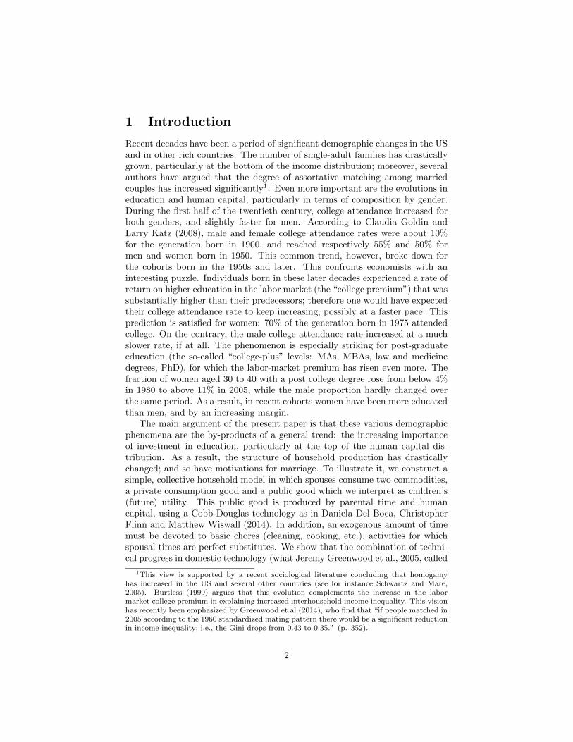
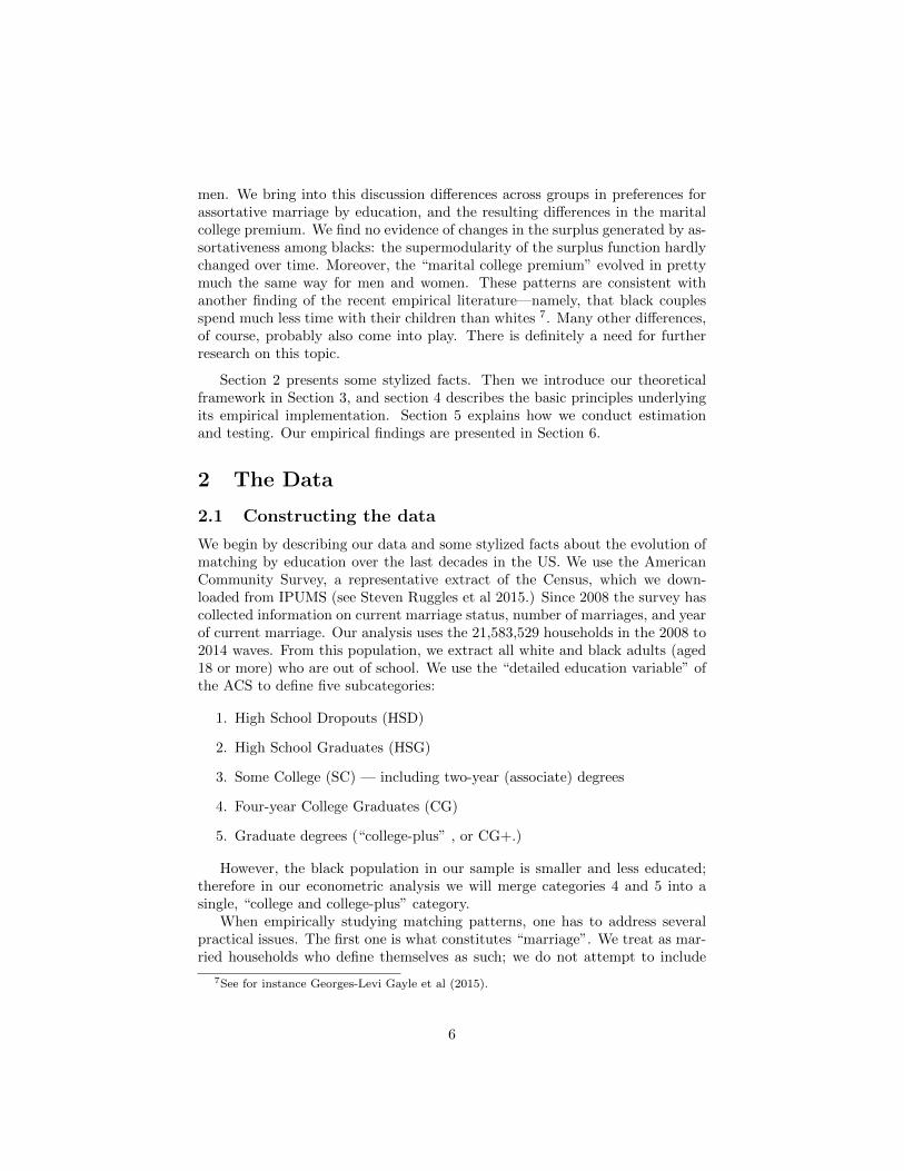
The trends in education levels of white men and women are shown in figures 1and 2. In cohorts born after 1955, women are more likely than men to attend col-lege; for those born after 1965, they are also more likely to achieve a college-plusdegree. Not coincidentally, the proportion of marriages in which the husband

12Recall that these are first unions.

8

1940 1945 1950 1955 1960 1965 1970

0.0

0.1

0.2

0.3

0.4

0.5

0.6

Year of birth

Pro

port

ion

HSD −−− MenHSD −−− WomenHSG −−− MenHSG −−− WomenSC −−− MenSC −−− WomenCG −−− MenCG −−− WomenCG+ −−− MenCG+ −−− Women

Figure 1: Educations of white men and women

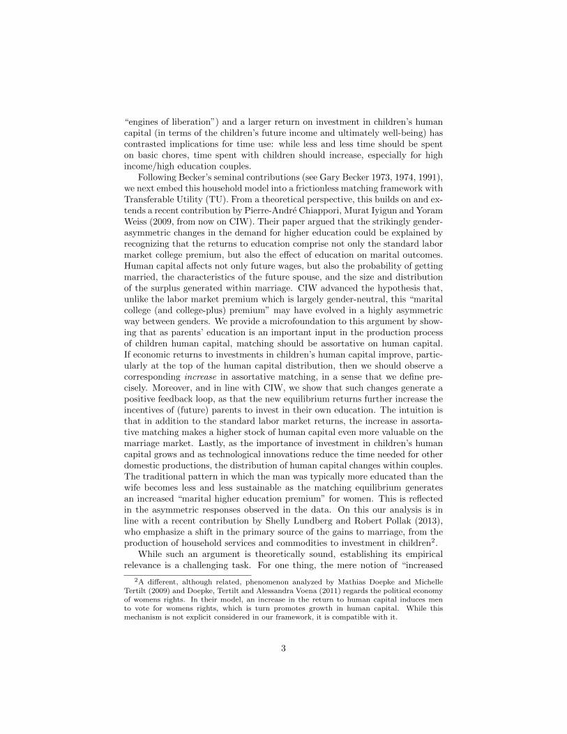
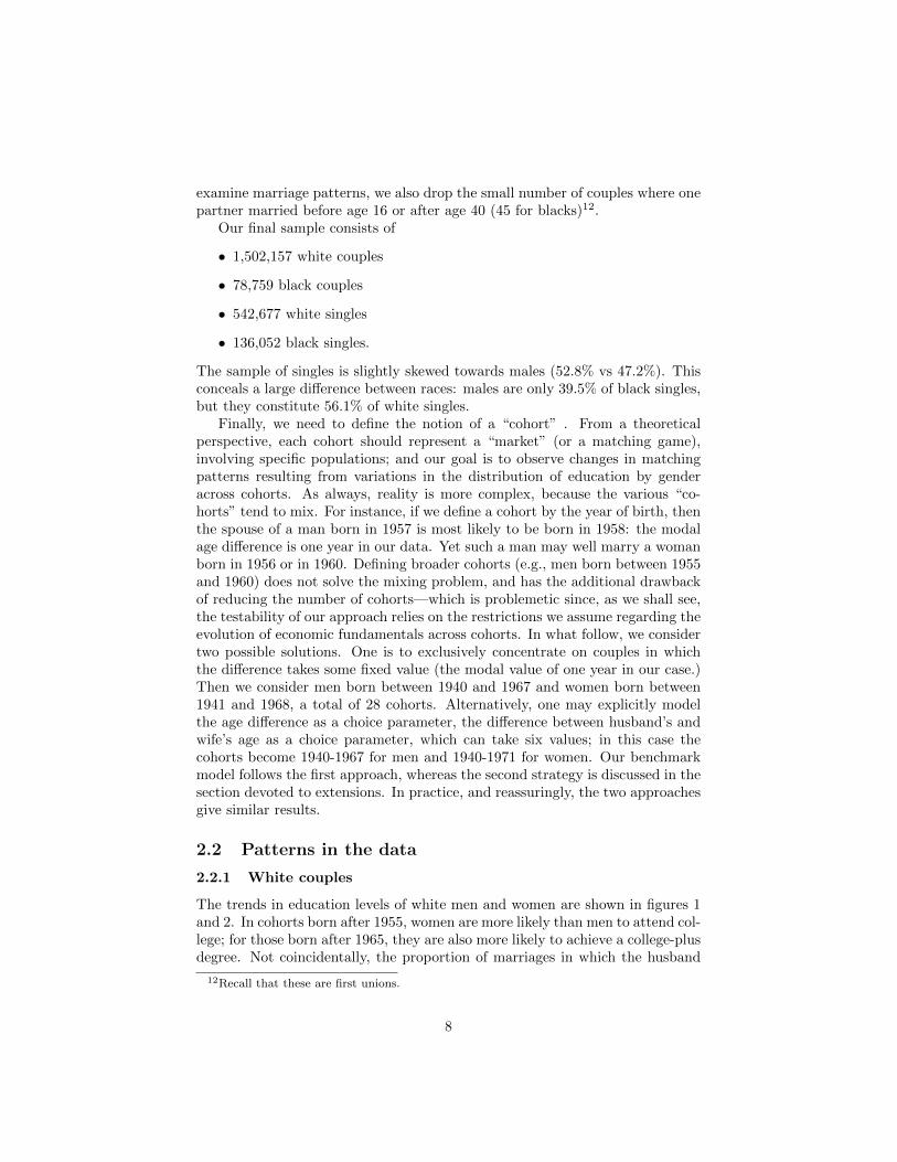
is more educated than the wife has fallen quite dramatically. Indeed, Figure 2shows that the percentage of couples in which spouses have the same educationis remarkably stable (slightly below 50%) over more than three decades. How-ever, there are now more couples in which the wife is more educated than theopposite.

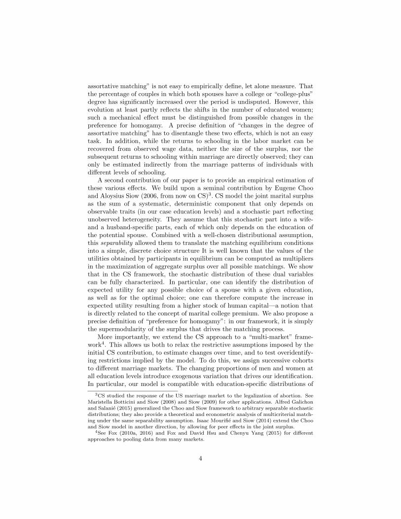
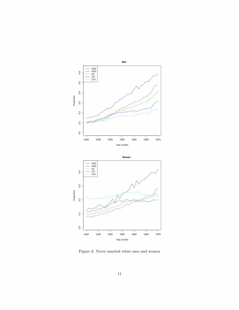
Figure 3 illustrates the decline in marriage among whites by plotting thepercentage of individuals who never married by cohort and education. Theyshow that, for both genders, a higher education has tempered the decline inmarriage; high-school dropouts, on the other hand, have faced a very steepdecline in marriage rates. However, female patterns are very specific. For theolder cohorts of our sample, a college-plus degree had a strong, negative effecton the probability of getting married for women, but not for men. This genderdifference has largely disappeared in recent cohorts: college-plus women nowmarry as much as college graduates, and much more than high-school educatedwomen.

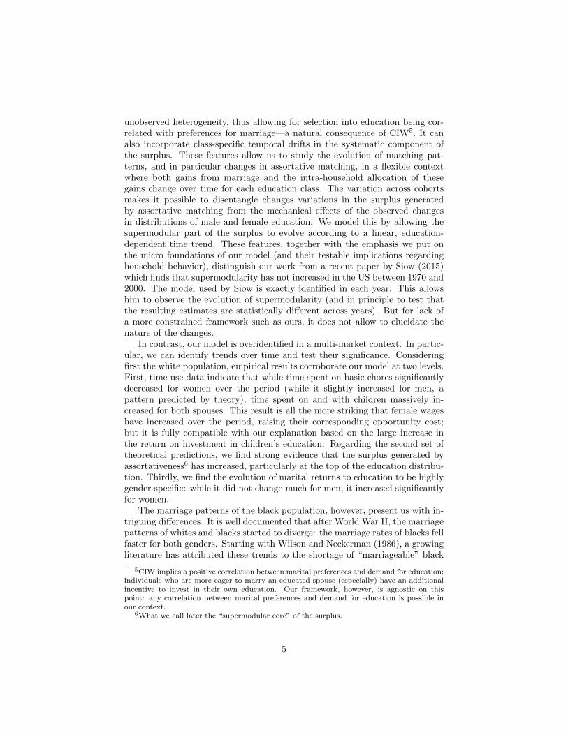
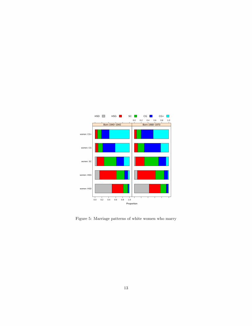
Figures 4 and 5 describe marital patterns by education. They show thatcollege-educated men are now much less likely to “marry down” (about 25%,against 50% for men born in the early 40s). The pattern for women is opposite;for instance, the proportion of college-educated women who marry up (with acollege-plus husband) has dropped from 40% to 20% over the period.

9

1940 1945 1950 1955 1960 1965 1970

0.0

0.1

0.2

0.3

0.4

0.5

0.6

0.7

Year of birth of husband

Pro

port

ion

Husband more educatedSame educationHusband less educated

Figure 2: Comparing partners in white couples

10

1940 1945 1950 1955 1960 1965 1970

0.0

0.1

0.2

0.3

0.4

0.5

0.6

Year of birth

Pro

port

ion

HSDHSGSCCGCG+

Men

1940 1945 1950 1955 1960 1965 1970

0.0

0.1

0.2

0.3

0.4

Year of birth

Pro

port

ion

HSDHSGSCCGCG+

WomenText

Figure 3: Never married white men and women

11

Proportion

men: HSD

men: HSG

men: SC

men: CG

men: CG+

0.0 0.2 0.4 0.6 0.8 1.0

Born 1940−1942

0.0 0.2 0.4 0.6 0.8 1.0

Born 1968−1970

HSD HSG SC CG CG+

Figure 4: Marriage patterns of white men who marry

12

Proportion

women: HSD

women: HSG

women: SC

women: CG

women: CG+

0.0 0.2 0.4 0.6 0.8 1.0

Born 1940−1942

0.0 0.2 0.4 0.6 0.8 1.0

Born 1968−1970

HSD HSG SC CG CG+

Figure 5: Marriage patterns of white women who marry

13

2.2.2 Black couples

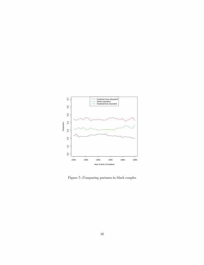
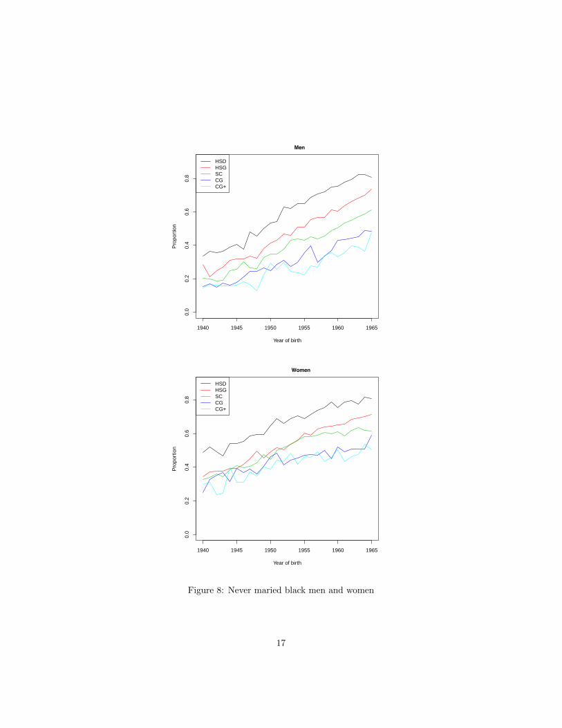
The education and marriage patterns of blacks show some striking differencesfrom whites. Black women have always been at least as likely as men to get acollege or a college-plus degree; and in contrast with the white population, theproportions of a cohort with at least a college degree evolve in a very similarway for men and for women (figure 6.) Figure 7 shows that in striking con-trast to white couples, in black couples it has always been more likely that thewoman was more educated; and this difference has increased in recent years. inSecondly, marriage rates have declined much faster for blacks than for whites(see figure 8.) For the cohorts born in the mid 60s, the fraction of never mar-ried at age 45 is above 40% for all education classes, and exceeds 80% for highschool drop-outs. Thirdly, for the older cohorts, one does not observe the samedifference between genders as for whites. While the percentage of couples withequal education are similar for blacks and whites (a stable proportion around45%), in unequally educated couples the wife is always more likely to be themore educated person among blacks. Finally, the proportion of college educatedindividuals who never marry was much larger for men than women in the oldercohorts; recent percentages are quite similar. In other words, the spectaculardifferences across genders that characterize the white population cannot be seenin the African-American sample13.

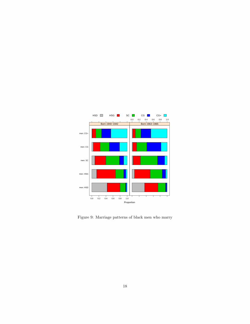
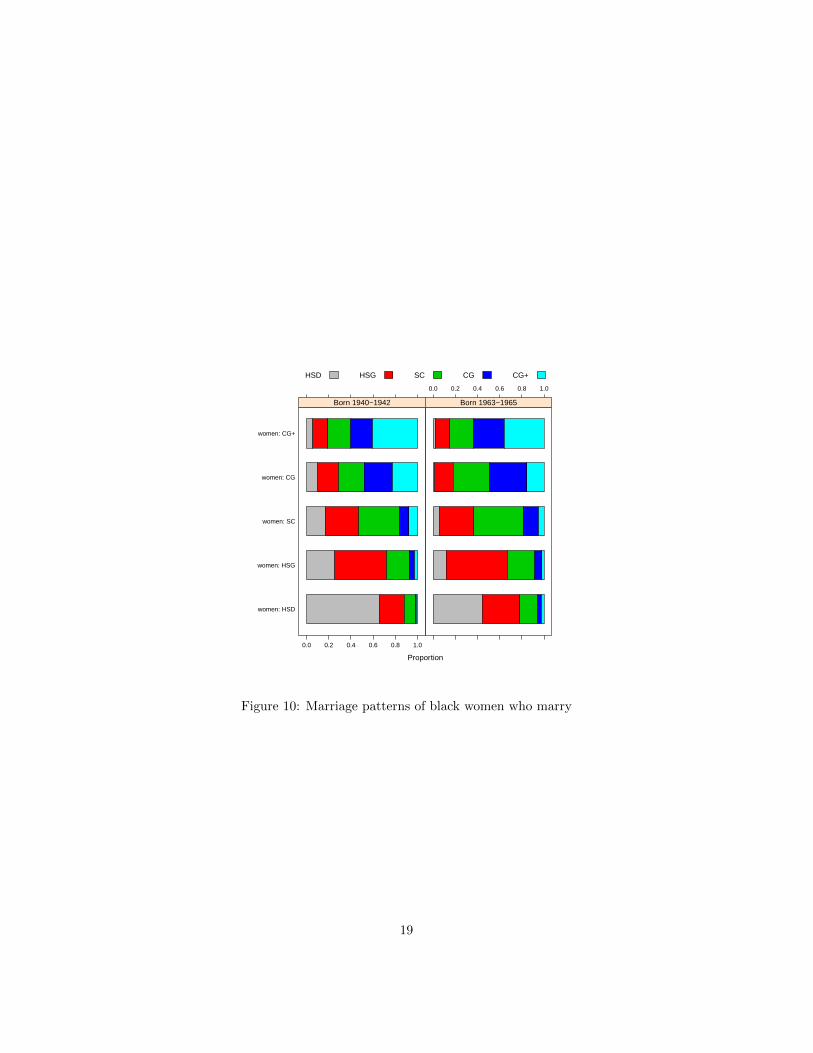
It is also worth noting that the marital patterns by education of black menand women who do marry are not that different from those of whites (compareFigures 9 and 10 to Figures 4 and 5.) The main difference is that fewer men“marry down” in the black population.

* * * *

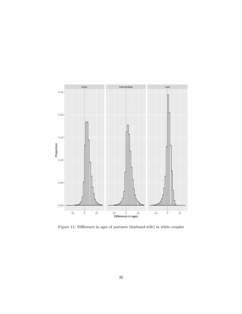
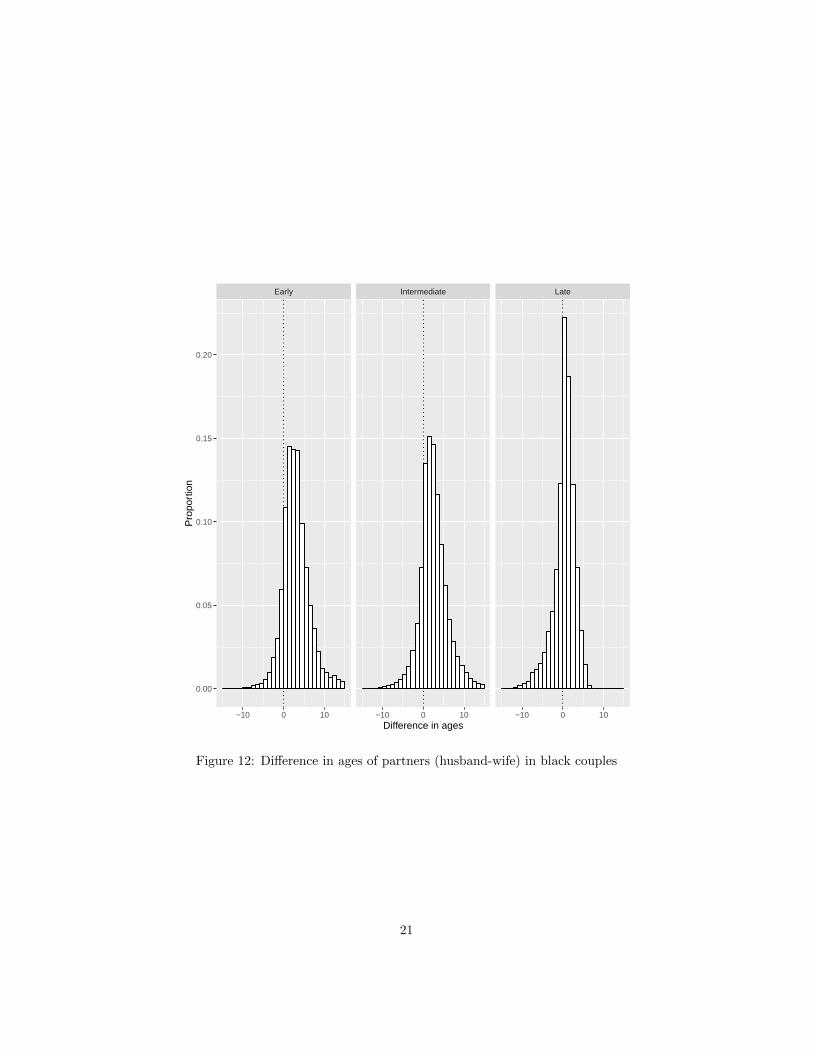
Finally, the evolution of age differences between spouses for the white andblack populations is shown in Figures 11 and 12, where “early” and “late”refer to the first and the last three cohorts respectively. The age difference hasdecreased slowly over time. Men are still more likely to be the older partner; butcouples in which the woman is older are quite common in more recent cohorts(29% of white couples and 33% of black couples are to the left of the dashedline in the rightmost panel.) The proportion of couples in which the (absolute)age difference is larger than ten years has become very small.

A large literature has evaluated the changes in the value of a higher edu-cation on the labor market. While this labor market college premium seemsto have evolved in very similar ways across genders and races, the patternsdocumented here clearly suggest that the effects of a higher education on mari-tal prospects have diverged much more. Yet descriptive statistics alone cannotmeasure changes in the joint surplus of matches and in its division between the

13We should also note here the increase in interracial marriages that started around 1960and accelerated recently. Black men are much more likely than black women to marry a whitespouse—see Gullickson (2006) and Cherlin (1992, Chapter 4.) Our model does not considerthese additional dimensions, which were less prominent in our sample period.

14

1940 1945 1950 1955 1960 1965

0.0

0.1

0.2

0.3

0.4

0.5

0.6

Year of birth

Pro

port

ion

HSD −−− MenHSD −−− WomenHSG −−− MenHSG −−− WomenSC −−− MenSC −−− WomenCG −−− MenCG −−− WomenCG+ −−− MenCG+ −−− Women

Figure 6: Educations of black men and women

15

1940 1945 1950 1955 1960 1965

0.0

0.1

0.2

0.3

0.4

0.5

0.6

0.7

Year of birth of husband

Pro

port

ion

Husband more educatedSame educationHusband less educated

Figure 7: Comparing partners in black couples

16

1940 1945 1950 1955 1960 1965

0.0

0.2

0.4

0.6

0.8

Year of birth

Pro

port

ion

HSDHSGSCCGCG+

Men

1940 1945 1950 1955 1960 1965

0.0

0.2

0.4

0.6

0.8

Year of birth

Pro

port

ion

HSDHSGSCCGCG+

Women

Figure 8: Never maried black men and women

17

Proportion

men: HSD

men: HSG

men: SC

men: CG

men: CG+

0.0 0.2 0.4 0.6 0.8 1.0

Born 1940−1942

0.0 0.2 0.4 0.6 0.8 1.0

Born 1963−1965

HSD HSG SC CG CG+

Figure 9: Marriage patterns of black men who marry

18

Proportion

women: HSD

women: HSG

women: SC

women: CG

women: CG+

0.0 0.2 0.4 0.6 0.8 1.0

Born 1940−1942

0.0 0.2 0.4 0.6 0.8 1.0

Born 1963−1965

HSD HSG SC CG CG+

Figure 10: Marriage patterns of black women who marry

19

Early Intermediate Late

0.00

0.05

0.10

0.15

0.20

0.25

−10 0 10 −10 0 10 −10 0 10Difference in ages

Pro

port

ion

Figure 11: Difference in ages of partners (husband-wife) in white couples

20

Early Intermediate Late

0.00

0.05

0.10

0.15

0.20

−10 0 10 −10 0 10 −10 0 10Difference in ages

Pro

port

ion

Figure 12: Difference in ages of partners (husband-wife) in black couples

21

partners; a more precise evaluation of this “marital college premium” requiresan explicit structural model.

3 Theoretical Framework

Our model derives from CIW, who consider an economy with two periods andlarge numbers of men and women. In period one, agents draw costs of invest-ment in human capital and marital preferences from some random distributions;then they invest in education by choosing from a finite set of possible educationallevels. In period 2, agents match on a frictionless marriage market with trans-ferable utility; they each receive a wage, the realization of which depends onthe agent’s education; and they consume according to an allocation of resourcesthat was part of the matching agreement.

When investing in human capital, agents must anticipate the outcome oftheir investment. This outcome has two distinct components. One is a largerfuture wage. In our framework, this effect is taken to be exogenous, and tobenefit single and married agents alike. Second, a higher educational level hasan impact on marital prospects; it affects the probability of getting married,the expected income of the future spouse, the total utility generated withinthe household, and the intra-couple allocation of this utility. These maritalgains, however, depend on the equilibrium reached on the marriage market;this in turn depends on the distribution of education in the two populations,and ultimately of the investment decisions made in the first period. As usual,the model can be solved backwards using a rational expectations assumption;equilibrium is reached when the marital gains resulting from given distributionsof education for men and women trigger first period investment decisions thatexactly generate these distributions. Note that even if marital preferences andinvestment cost were independent ex ante, education decisions made during thefirst period must be correlated with preferences for marriage ex post: sinceagents with stronger preferences for marriage are more likely to receive themarital gain than agents who prefer to stay single, they have stronger incentivesto invest in education.

In the present paper, we aim at estimating and testing the second periodbehavior described by this model. This choice is mostly dictated by availabledata: while private costs of human capital investment are not observable, theresulting distribution of education by gender is. In addition, concentrating onthe second period allows to introduce a slightly more general framework whileaddressing the empirical content of the key theoretical concept: the notion of amarital college premium. We therefore consider the situation at the beginningof the second period. Agents are each characterized by their chosen level of ed-ucation, which belongs to some finite set and is observable by all, and by theirpreferences for marriage, which are observed by their potential mates but notby the econometrician. Our goal is to identify the underlying structure fromobserved matching patterns; and we are particularly interested in the maritalgains associated with each educational level. Lastly, and as explained in the in-

22

troduction, we follow the literature14 by assuming that the utility of each agentis the sum of a deterministic component, which reflects the agent’s consump-tion and investment choices, and a non economic shock reflecting the agent’sidiosyncratic marital preferences.

3.1 Preferences: the economic component

The economy consists of a male population M and a female population F ,who differ only by their human capital. Education is the outcome of individualchoices made before the matching stage. At the beginning of the matching game,which we consider here, these classes are therefore considered by the agents asexogenously given. However, the outcome of the matching game will, in equi-librium, impact the investment decision; this is the gist of CIW’s contribution.

3.1.1 Producing children’s human capital

In our model, the primary purpose of marriage is the production of a publicgood, namely children’s (future) welfare. For simplicity, we assume that eachcouple has exactly one child. We are mostly interested here in human capitalaccumulation; therefore we assume that a child’s future well being is a functionof the child’s human capital Q:

UC = Qα

where α is a parameter summarising the impact of human capital on the child’sfuture wages, income dynamics and ultimately welfare.

For simplicity, we assume that each couple has one child. The child’s humancapital is produced using parental time; other inputs could be introduced with-out changing the main conclusions. Following the recent literature on humancapital production, we assume that the impact of parental time is proportionalto the parent’s own human capital, and that mother’s and father’s time inputsare complement in the production of the child’s human capital.15 In practice,we use a Cobb-Douglas form:

Q = (H1t1)β

(H2t2)1−β

where Hi and ti respectively denote parent i’s human capital and time spentwith the child.

Alternatively, agents may use available time to work on the market or toaccomplish domestic chores. On the labor market, an agent’s wage is directlyproportional to her human capital:

wi = WHi

14See for instance Chiappori and Salanie (2016) for a survey.15Recent work incorporating such complementarities include del Boca, Flinn and Wiswall

(2012).

23

where W is some aggregate shock. We assume for simplicity that chores requiresome fixed amount of time τ ′, for which male and female time are perfect sub-stitutes; and that they involve no human capital. As a result, chores will beentirely performed by the spouse with a lower market wage, whom we numberas spouse 2. The spouses’ respective time constraints are therefore:

t1 + l1 = 1 and t2 + l2 = τ = 1− τ ′

where li denotes i’s market work and τ is total time available for agent 2.

3.1.2 Preferences, surplus and individual welfare

Continuous version Individual utilities consist of an economic and a noneconomic, predetermined component. The economic component depends onprivate and public consumptions according to a Cobb-Douglas form:

ui (qi, UC) = qiUC = qiQα

where qi denotes i’s private consumption. The couple’s budget constraint istherefore:

q1 + q2 = WH1 (1− t1) +WH2 (τ − t2)

or equivalently

q1 + q2 +WH1t1 +WH2t2 = (H1 + τH2)W (1)

These Cobb-Douglas preferences are of the Bergstrom and Cornes’ gener-alized quasilinear form16; therefore they imply transferable utility. It followsthat any efficient allocation maximizes the sum of utilities under the budgetconstraint:

G (H1, H2) = max (q1 + q2)Qα

under (1). The solution is:

H1t1 =αβ

1 + α(H1 + τH2) , H2t2 =

α (1− β)

1 + α(H1 + τH2) (2)

and q1 + q2 =1

1 + α(H1 + τH2)W.

In particular, we see that both t1 and t2 are increasing in α and in τ . That is,the larger the importance of children’s human capital for their future welfare, themore time both parents will invest in producing this human capital. Moreover,a reduction in the time devoted to chores, by raising total available time τ , willhave the same impact. Also note that the value of the sum of utilities at theoptimum is

G (H1, H2) = K (H1 + τH2)1+α

W

16See Ted Bergstrom and Richard Cornes (1983).

24

where

K =ααβαβ (1− β)

α(1−β)

(1 + α)1+α

Similarly, let Gi (Hi), i = 1, 2, denote the utility of person i when single, sothat the economic surplus generated by marriage is

S (H1, H2) = G (H1, H2)−G1 (H1)−G2 (H2) .

It follows that:

∂2S (H1, H2)

∂H1∂H2=∂2G (H1, H2)

∂H1∂H2= α (1 + α) τKW (H1 + τH2)

α−1> 0 (3)

We conclude that the function S is supermodular in the spouses’ human cap-ital. In particular, in the absence of the non-monetary component of individualutilities, matching should be strictly positive assortative on human capital.

Lastly, equilibrium conditions determine the surplus allocation between spouses.Specifically, let U (H1) and V (H2) respectively denote, in a couple (H1, H2),the share of surplus received by spouse 1 and 2. Feasibility implies that:

U (H1) + V (H2) = S (H1, H2)

while stability requires that for all (H ′1, H′2):

U (H1) + V (H2) ≥ S (H ′1, H′2) .

It follows thatU (H1) = max

H2

(S (H1, H2)− V (H2))

and by the envelope theorem:

U ′ (H1) =∂S

∂H1(H1, H2) .

This expression becomes

U ′ (H1) = (α+ 1)KW (H1 + τH2)α

and similarlyV ′ (H2) = τ (α+ 1)KW (H1 + τH2)

α.

These derivatives are important because they represent the additional gaingenerated, in the marriage market, by a marginal increase in the stock of humancapital. As such, they determine individuals’ incentives to invest in their ownhuman capital. We see that

U ′ (H1)

V ′ (H2)=

1

τ> 1.

25

In other words, the presence of chores implies that the spouse whose wage willbe higher has stronger marginal incentives to invest in education - although anincrease in τ tends to reduce the discrepancy. In that sense, the equilibriumis, as argued above, “self-reinforcing”: in a world in which one gender is moreeducated, the equilibrium logic results in stronger incentives to invest for thatgender, which tends to reinforce the asymmetry. Equilibrium phenomena tendtherefore to exacerbate initial differences, typically resulting in strong responsesto even minor changes in the economic context.

Discrete version In the empirical application below, individual human capi-tal will be proxied by the person’s education. In practice, thus, each individual ibelongs to an education class I = 1, . . . ,K which is observed by the econometri-cian. Let therefore SIJ denote the economic surplus generated by the matchingof spouses with respective educations I and J .

To measure supermodularity with discrete types, cross derivatives must be

replaced with cross differences. In practice, we call a 2 × 2 matrix

(a bc d

)supermodular if a + d − b − c ≥ 0. Then the K × K matrix S is supermodularif all its 2× 2 submatrices are supermodular.

Equivalently,we may define the cross-difference operator DIJ,KL by:

DIJ,KL (A) = AIJ +AKL −AIL −AKJ (4)

for any matrix A. Then supermodularity has a simple translation: for all(I, J,K,L), if I < K and J < L then DIJ,KL (A) > 0.

In particular, one can define the supermodular core of the surplus matrix Sas the array

D (S) =(DIJ,KL (S) , I,K = 1, ...,K, J, L = 1, . . . ,K, I < K, J < L

)(5)

Then the surplus is supermodular if and only if all components of its supermod-ular core are positive (this is very similar to the definition in Siow 2015.)

3.1.3 Comparative statics: general results

Driving forces The theoretical model presented above generates clear-cutcomparative statics results. As argued in the introduction, we concentrate ontwo major changes that affected household technology over the recent decades.One is the sustained rate of technological advance in the household sector—what Greenwood et al. (2005) call “engines of liberation”. Although the pro-cess started early (around the beginning of the twentieth century, for instance,for refrigerators), progress continued regularly since then. The latest wave oftechnological innovations includes dishwashers (whise current penetration rateis around 80% in the US, against 45% in 1990 and less than 10% in the sixties)and microwaves (which appeared in the 80s, for a current penetration rate over95%). Greenwood et al. convincingly argue that ‘technological progress in thehousehold sector played a major role in liberating women from the home’ (p.

26

109). In our model, the direct translation is a significant reduction of the timeτ ′ devoted to chores—or, equivalently, an increase in available time τ .

A second and major evolution is the increased importance of human capitalon wages and income. This trend is well summarized by Goldin and Katz (2009):

[. . . ] much of the rising wage inequality in recent history can betraced to rising differences between the wages of the highly educatedand the less educated17.

In other words, while a child’s future (expected) well-being has always beenan increasing function of the accumulated stock of human capital, this relation-ship is stronger and steeper now than it was fifty years ago. In our model, thedirect implication of this trend is that the coefficient α, which summarizes theimpact of human capital on future income and well-being, has increased signif-icantly over the period under consideration, at least for individuals reaching acollege degree and beyond.

Note, however, that the increased importance of human capital has a doubleeffect. Not only does it boost the returns on investment on children, but italso directly affects the link between the parents’ stock of human capital andthe wage they receive on the market. Again, the theoretical framework deliversprecise predictions regarding this impact. The parameter governing the rela-tionship between wages and human capital is the aggregate wage shock W ; inour comparative statics analysis, we shall therefore investigate the consequencesof an increase in W , particularly for more educated people.

Lastly, the higher level of female human capital implies that the opportu-nity cost of the time women devote to non market activities—both chores andchildren—is much higher. Moreover, in more and more couples the wife’s wageexceeds the husband. For instance, while the fraction of couples where husbandand wife have the same education has remained more or less constant, coupleswith a more educated wife now outnumber those exhibiting the opposite pattern;and in more than 20% of couples, the wife’s income exceeds the huband’s. Notethat these trends are by no means specific to the US; they affect all developedeconomies (and many developing ones as well).

Implied predictions: domestic time use Given our structural model,these evolutions should generate two types of testable consequences. A firstset of predictions can directly be tested on available data. According to ourframework, the allocation of time devoted to chores should globally decrease.Moreover, and given our assumption that male and female time are perfect sub-stitutes, the specialization patterns should somewhat shift, with less women andmore men devoting time to such domestic activities.

17Page 2. Goldin and Katz estimate that increases in the economic returns to investmentsin education from 1973 to 2005 account for about 60 percent of the rise in wage inequalityover that period. For a detailed analysis, see Goldin and Katz (2008)

27

Next, consider investment in children. A first prediction is that the timespent by the husband should increase. Indeed, efficiency implies that:

t1 =αβ

1 + α

(1 + τ

H2

H1

)which is increasing in α, τ and the ratio H2/H1 — all of which have increasedover the period — and is independent of the wage coefficient W . Regardingwomen, things are however more complex. Indeed, (2) now gives:

t2 =α (1− β)

1 + α

(H1

H2+ τ

)Here, t2 is increasing in α and τ and does not depend on W ; but it decreaseswith the ratio H2/H1. Therefore, women’s time spent with children will increaseonly if the first two effects—increased importance of these investments and moretime available—dominate the third, i.e. the shift in the education profile withincouples. All in all, we expect the increase (if any) to be smaller than for men.

Implied predictions: supermodularity and its evolution A second set ofpredictions relates to the evolution of matching patterns. Specifically, our modelgenerates a supermodular surplus. A natural question, therefore, is whetherthis supermodularity is strengthened or weakened by the various trends wejust described. To answer this question, let us first see how the second crossderivative—which sign determines super- or submodularity—changes with thekey parameters. (3) gives:

∂3S (H1, H2)

∂τ∂H1∂H2=αα+1βαβW (H1 + τH2)

α−2(H1 + ατH2)

(α+ 1)α

(1− β)α(β−1) > 0

and

∂3S (H1, H2)

∂α∂H1∂H2=βαβαα+1τW (H1 + τH2)

α−1

(1− β)α(β−1)

(α+ 1)α

(ln (H1 + τH2) + L (α, β))

where

L (α, β) =2α+ 1

α (α+ 1)+ ln

α

α+ 1+ ln

((1− β)

1−βββ)

It follows that an increase in τ always makes the surplus function S more su-permodular. So does an increase in α, since the expression L (α, β) is alwayspositive for α, β ∈ [0, 1]. Moreover, these impacts are larger, the higher thecouples’ levels of human capital. Lastly, what about the wage component W?Again,

∂3S (H1, H2)

∂W∂H1∂H2= α (1 + α) τK (H1 + τH2)

α−1> 0

and we conclude that an increase in the market reward to human capital (assummarized by the factor W ) also increases the supermodularity of the surplus.

28

Differences by human capital Lastly, an implicit assumption of the pre-vious exercise in comparative statics is that the importance of human capital(either for children, as summarized by the coefficient α, or for parental wages,as indicated by the wage coefficient W ) has increased uniformly for all ed-ucational levels. In practice, the impact is mostly visible at the top of thedistribution. The college and college-plus premiums have drastically increasedsince the 80s.According to David Autor (2014), the earnings gap between themedian high-school educated and college-educated US males working full-year,full-time jobs doubled between 1979 and 201218. On the contrary, the return toeducation at a lower level (say, between high-school drop-out and high-schoolgraduate) have probably increased much less, if at all. While an exact quantifi-cation is plagued with selection issues, Lawrence Mishel et al. (2013) estimatethat the “high school premium” remained fairly stable (between 20 and 25%)over the same period. Similarly, raw data indicate (again without controlingfor selection) that the wage difference between high school graduates and “somecollege” actually declined over the same period. This strongly suggests that theimportance of investment in human capital has increased more for high humancapital couples, making our ui functions more convex in Q and increasing morethe wage factor W at the top of the distribution of education. Therefore ourcomparative statics conclusions should apply with more force at the top thanat the bottom of the distribution.

The discrete setting While the first set of predictions, which regard intra-household allocation of domestic time, can readily be tested, the predictions re-garding assortative matching must be translated into our discrete setting. Thecrucial tool, here, is the supermodular core matrix defined in (4) and (5). Inparticular, we submit that the somewhat vague notion that “assortative match-ing creates more surplus now than it used to in the past” should be formallydefined as follows. Suppose that we observe the surplus matrix S over two pe-riods, T = 1 and T = 2; in particular, we can compute the supermodular corematrix D (S) at each period. Then

Definition 1 (Additional surplus generated by assortativeness)The surplus generated by assortativeness does not change between T = 1 and

T = 2 if and only if the matrix D (S) is the same at T = 1 and T = 2.The surplus generated by assortativeness increases if and only if all compo-

nents of the matrix D (S) increase between T = 1 and T = 2; equivalently, thematrix (S2 − S1) is supermodular.

Note that this definition is of independent interest: it provides an explicitcharacterization of the somewhat hazy notion of “increased preferences for as-sortativeness” - which, in our context, corresponds to changes in the additionalsurplus generated by assortativeness. Moreover, this characterization is struc-tural: it relies on a model in which assortativeness is related to supermodularity

18From 17, 000 to 34, 000 constant 2012 dollars.

29

of the surplus function (a natural link indeed), and exploits this relationship toprovide a formal definition.

Lastly, the definition can be applied for some categories only. For instance,we shall say that the additional surplus generated by assortativeness has in-creased for educated people (say, individuals at education level L and above)if the corresponding, (K − L)× (K − L) submatrix of S exhibits the property -that is, if all components of the matrix

D (S) =(DIJ,KL (S) , I,K = L, ...,K, J, L = L, . . . ,K, I < K, J < L

)(6)

increase between T = 1 and T = 2. Equivalently, if matrix SLc is defined by:

SLc =((SIJc

)), I,K = L, ...,K

then the matrix SLc′ − SLc is supermodular for c′ > c.In particular, the previous, comparative statics results predict that the ad-

ditional surplus generated by assortativeness, defined as above, must have in-creased over the period, particularly for higher levels of education. In practice,if we estimate the economic surplus matrix SLc over two periods, c and c′, withc < c′, the matrix SLc′ − SLc should be supermodular for L ‘large enough’.

3.2 Preferences: non monetary component

In addition to (economic) preferences over commodities, each individual hasnon-monetary marital preferences which we model by random vectors. FollowingChoo and Siow (2006), we assume that an individual preferences over potentialspouses are individual-specific and only depend on the spouse’s education class.For instance, a woman j belonging to class J has a vector of marital preferences

bJj =(b∅Jj , b1Jj , ..., bKJj

)where bKJj denotes the utility j derives from marrying a spouse with an educa-

tion K (and where, by convention, b∅Jj denotes the utility j derives from stayingsingle). Similarly, man i’s idiosyncratic marital preferences are described by thevector

aIi =(aI∅i , a

I1i , ..., a

IKi

)where I denotes i’s education. Note that the distribution of an individual’svector of marital preferences may depend on the individual’s own education;more educated men may, on average, value differently an educated wife thanless educated men. Not only is this assumption quite plausible empirically, butit is also needed to reflect the endogeneity of education. In CIW, for instance,individual tastes for marriage influence investment in education, because theyaffect the probability that an individual reaps the benefits of education on themarriage market. Since individuals with different marital tastes invest differ-ently, the conditional distribution of taste given education will typically vary

30

with education, reflecting the selection into educational choices. Consequently,we define

AIJ = E(aIJi |i ∈ I

)and BIJ = E

(bIJj |j ∈ J

).

It should be stressed that, in this framework, these idiosyncratic, additively sep-arable shocks are the only source of unobserved heterogeneity. This assumptionis crucial in order to apply the Choo-Siow approach; see Chiappori and Salanie(2015) for a detailed discussion.

Finally, and still following Choo and Siow (2006), we assume that economicand marital preferences are additively separable. To be more precise, the maritalsurplus sij generated by the match of man i with education I and woman jwith education J is the sum of two components. One is the expected economicsurplus SIJ , generated by joint consumption; the other consists of the sum ofthe spouses’ idiosyncratic preferences for marriage with each other, relative tosinglehood.

sij = SIJ + (aIJi − aI∅i ) + (bIJj − b∅Ji ). (7)

or, using the previous definitions:

sij =(SIJ + (AIJ −AI∅) + (BIJ −B∅J)

)+(

(aIJi −AIJ)− (aI∅i −AI∅))

+(

(bIJj −BIJ)− (b∅Jj −B∅J)).

The component on the first line

ZIJ = SIJ + (AIJ −AI∅) + (BIJ −B∅J) (8)

is, by construction, the conditional expectation of the total surplus for matchesbetween classes I and J . Within it, SIJ is the conditional expected economicsurplus, while (AIJ − AI∅) + (BIJ − B∅J) represents the conditional expectedsurplus from marital preferences. By definition, the components on the last twolines have zero expectation across all hypothetical matches. We use

αIJi = aIJi −AIJ and βIJj = bIJj −BIJ

to denote the within-class variation of marital preferences; note that, by con-struction,

E[αIJi

]= E

[βIJj

]= 0 for all i, j, I, J

Finally, the total surplus generated by the match between i ∈ I and j ∈ J is:

sij = ZIJ +(αIJi − αI∅i

)+(bIJj − b∅Jj

)(9)

The matrix Z =(ZIJ

)will play a crucial role in what follows. As we shall

see, the equilibrium matching will depend on preferences through the matrix Zand the distribution of the α’s and β’s. From the definitions above, ZIJ reflects

31

the distribution of income and preferences over commodities of spouses whochose education levels I and J (and each other), as well as the distribution oftheir marital preferences. It is therefore a complex object; but it is the crucialconstruct that determines marital patterns in our context. Our goal is to checkunder which conditions it is identifiable from observed matching patterns.

3.3 Matching

A matching consists of

(i) a measure dµ on the set M× F , such that the marginal of dµ over M(resp. F) is dµM (dµF ); and

(ii) a set of payoffs (or imputations) ui, i ∈M and vj , j ∈ F such that

ui + vj = zij for any (i, j) ∈ Supp (dµ)

In words, a matching indicates who marries whom (note that the allocationmay be random, hence the measure), and how any married couple shares thesurplus zij generated by their match. The numbers ui and vj are the expectedutilities man i and woman j get on the marriage market, on top of their utilitieswhen they remain single; for any pair that marries with positive probability,they must add up to the total surplus generated by the union.

3.3.1 Stable Matchings

A matching is stable if one can find neither a man i who is currently married butwould rather be single, nor a woman j who is currently married but would ratherbe single, nor a woman j and a man i who are not currently married together butwould both rather be married together than remain in their current situation.Formally, we must have that:

ui ≥ 0, vj ≥ 0 and (10)

ui + vj ≥ zij for any (i, j) ∈M×F . (11)

The two conditions in (10) implies that married agents would not prefer remain-ing single; the third (condition (11)) translates the fact that for any possiblematch (i, j), the realized surplus zij cannot exceed the sum of utilities respec-tively reached by i and j in their current situation (i.e., a violation of thiscondition would imply that i and j could both strictly increase their utility bymatching together).

As is well known, a stable matching of this type is equivalent to a maxi-mization problem; specifically, a match is stable if and only if it maximizes totalsurplus,

∫zdµ, over the set of measures whose marginal over M (resp. F) is

dµM (resp. dµF ). A first consequence is that existence is guaranteed under mildassumptions. Moreover, the dual of this maximization problem generates, foreach man i (resp. woman j), a dual variable or “shadow price” ui (resp. vj),

32

and the dual constraints these variables must satisfy are exactly (10): the dualvariables exactly coincide with payoffs associated to the matching problem.

Finally, note that with finite populations, the payoffs ui and vj are notuniquely defined: they can be marginally altered without violating the (finite)set of inequalities (10). However, when the populations become large, the inter-vals within which ui and vj may vary typically shrink; in the limit of continuousand atomless populations, (the distributions of) individual payoffs are exactlydetermined. On all these issues, the reader is referred to Chiappori, McCannand Nesheim (2009) for precise statements.

3.3.2 A basic lemma

From an economic perspective, our main interest lies in the dual variables u andv. Indeed, vj is the additional utility provided to woman j by her equilibriummarriage outcome. While this value is individual-specific (it depends on Mrs.j’s preferences for marriage), its expected value conditional of j having reacheda given level of education J is directly related to the marital premium associatedwith education J (more on this below).

In our context, there exists a simple and powerful characterization of thesedual variables; it is given by the following Lemma:

Lemma 2 For any stable matching, there exist numbers U IJ and V IJ , I =1, ...,M, J = 1, ..., N , with

U IJ + V IJ = ZIJ (12)

satisfying the following property: for any matched couple (i, j) such that i ∈ Iand j ∈ J ,

ui = U IJ + (αIJi − α0Ji )

and (13)

vj = V IJ + (βIJj − β0Jj )

Proof. Assume that i and i′ both belong to I, and their partners j and j′ bothbelong to J . Stability requires that:

ui + vj = ZIJ + (αIJi − α0Ji ) + (βIJj − β

0Jj ) (14)

ui + vj′ ≥ ZIJ + (αIJi − α0Ji ) + (βIJj′ − β

0Jj′ ) (15)

ui′ + vj′ = ZIJ + (αIJi′ − α0Ji′ ) + (βIJj − β

0Jj ) (16)

ui′ + vj ≥ ZIJ + (αIJi′ − α0Ji′ ) + (βIJj′ − β

0Jj′ ) (17)

Subtracting (1) from (2) and (4) from (3) gives

(βIJj′ − β0Jj′ )− (βIJj − β

0Jj ) ≤ vj′ − vj ≤ (βIJj′ − β

0Jj′ )− (βIJj − β

0Jj )

hencevj′ − vj = (βIJj′ − β

0Jj′ )− (βIJj − β

0Jj )

33

It follows that the difference vj − (βIJj − β0Jj ) does not depend on j, i.e.:

vj − (βIJj − β0Jj ) = V IJ for all i ∈ I, j ∈ J

The proof for ui is identical.

In words, Lemma 1 states that the dual utility vj of woman j, belongingto class J and married with a husband in education class I, is the sum of twoterms. One is woman j’s idiosyncratic preference for a spouse with education Iover singlehood, βIJj −β

∅Jj ; the second term, V IJ , only depends on the spouses’

classes, not on who they are. In terms of surplus division, therefore, the U IJ

and V IJ denote how the deterministic component of the surplus, ZIJ , is dividedbetween spouses; then a spouse’s utility is the sum of their share of the commoncomponent and their own, idiosyncratic contribution.

Finally, for notational consistency, we define U I∅ = V ∅J = 0 ∀I, J .

3.3.3 Stable matching: a characterization

An immediate consequence of Lemma 1 is that the stable matching has a simplecharacterization in terms of individual choices:

Proposition 3 A set of necessary and sufficient conditions for stability is that

1. for any matched couple (i ∈ I, j ∈ J) one has

αIJi − αIKi ≥ U IK − U IJ for all K = ∅, 1, ..., N (18)

andβIJj − β

KJj ≥ V KJ − V IJ for all K = ∅, 1, ..., N (19)

2. for any single man i ∈ I one has

αIJi − αI∅i ≤ −U IJ for all J (20)

3. for any single woman j ∈ J one has

βIJj − β∅Jj ≤ −V IJ for all J (21)

Proof. See Appendix A.

Stability thus readily translates into a set of inequalities in our framework;and each of these inequalities relates to one agent only. This property is crucial,because it implies that the model can be estimated using standard statisticalprocedures applied at the individual level, without considering conditions oncouples. This separation is possible because the endogenous factors U IJ andV IJ adjust to make the separate individual choices consistent with each other.

34

3.4 Interpretation and comparative statics

3.4.1 The marital college premium

Labor economists define the “college premium” as the percentage increase in thewage rate that can be expected from a college education. This wage premiumcan readily be measured using available data, after controlling for selection intocollege; existing work suggests that, at the first order, it is similar for singlesand married persons and for men and women19 . We used the PSID to estimatea simple Mincer equation, separately for each gender and race but without anyattempt to control for selection. Figure 13 shows the resulting estimates of thelabor market college premium for both genders, for whites and for blacks. Ourpaper is mostly concerned with changes in the college premium over time. Itis worth noting at this stage that these (admittedly coarse) estimates suggestthat if anything, the labor market college premium has increased more for menthan for women. Also note the striking discrepancy between whites and blacks,and in particular the decrease in the labor market value of a college degree forblack women over time.

CIW point out that in addition to this wage premium, there exists a maritalcollege premium: a college education enhances an individual’s marital prospects,via the probability of being married and the expected education (or income) ofthe spouse, but also the size of the surplus generated and its division withinthe couple. In other words, it is well-understood that college education bene-fits individuals in terms of higher wages, better career prospects, etc; but ourgoal here is to capture the additional benefits that college-educated individualsreceive on the marriage market.

The notions previously defined allow a clear definition of the marital collegepremium. Indeed, the surplus is computed as the difference between the totalutility generated within the couple and the sum of individual utilities of thespouses if single, thus capturing exactly the additional gains from educationthat only benefit married people. Regarding individual well-being, an intuitiveinterpretation of U IJ (or equivalently of V IJ) would be the following. Assumethat a man randomly picked in class I is forced to marry a woman belongingto class J (assuming that the populations are large, so that this small deviationfrom stability does not affect the equilibrium payoffs). Then his expected util-ity is exactly U IJ (the expectation being taken over the random choice of theindividual—therefore of his preference vector—within the class).

Note, however, that this value does not coincide with the average utility ofmen in class I who end up being married to women J in a stable matching.The latter value is larger than U IJ , reflecting the fact that agents choose theirspouses. The expected surplus of an agent with education I is in fact

uI = E maxJ=0,1,...,J

(U IJ + αIJ

),

where the expectation is taken upon the distribution of the preference shockα. In particular, this expected surplus depends on the distribution of the pref-

19See for instance Bronson (2014, Figure 3B).

35

Blacks

Men

Blacks

Women

Whites

Men

Whites

Women

0

40

80

120

Per

cent

Cohort

1941−50

1951−60

1961−70

The college premium is defined as the percentage differencebetween hourly wages after a 4-year college degree and afterhigh-schol graduation for an individual of age 35. The er-ror bars reresent 95% confidence intervals. Source: PSID,with help from George-Levi Gayle, Limor Golan, and AndresHincapie.

Figure 13: Estimated labor market college premia

36

erence shocks; it will be computed below under a specific assumption on thisdistribution.

4 Empirical implementation

We now describe the econometric model we shall take to data. Galichon andSalanie (2015) proved that separable models are just identified under the strongcondition that the econometrician has exact knowledge of the probability dis-tributions of α and β. This is an obvious weakness, since it implies that themodel is simply not testable from cross-sectional data. A crucial feature ofour approach is that we analyze multiple markets; in practice, we shall considerseveral cohorts indexed by c = 1, . . . , T and exploit the time variations in the ed-ucation profiles of the populations at stake. Such a setting, in principle, shouldallow us to relax some restrictions while still generating overidentification tests.

Our first task is to describe how the structural components of our statisticalframework evolve across cohorts. We start, as a benchmark, with an immediategeneralization of CS. We show that this benchmark version generates strongoveridentifying restrictions, and we describe a set of overidentification tests.This model fits the data well for the black population, but it is strongly rejectedfor whites. We then discuss several further extensions of the model, which wego on to test.

4.1 The benchmark version

4.1.1 The structural framework

In a static version of CS, the surplus generated by the match of man i, belongingto class I, with woman j, belonging to class J , takes the form:

zij = ZIJ +(αIJi − αI∅i

)+(βIJj − β

∅Jj

)In a multi-cohorts setting, it is natural to assume that the shocks are in-

dependent across cohorts. How the deterministic part ZIJ varies with time isless clear. Allowing the entire Z matrix to vary freely across cohorts wouldamount to independently repeating static versions of CS, with no gain in termsof testability. Our benchmark model, therefore, introduces category-specificdrifts, whereby the ZIJ terms vary according to:

ZIJc = ζIc + ξJc + ZIJ (22)

so thatzij,c = ZIJ + ζIc + ξJc +

(αIJi,c − αI∅i,c

)+(βIJj,c − β

∅Jj,c

)In practice, the drifts ζIc and ξJc capture possible changes over time in the

surplus generated by marriage. There are several reasons to expect the surplusto vary across periods. One is that technological innovations have drastically

37

altered the technology of domestic production, therefore the respective genderroles within the household (see Greenwood et al 2005.) Other important factorswere the evolution of fertility control, as emphasized by Michael (2000) andGoldin and Katz (2002) among others; and improvements in medical techniquesand in infant feeding (Albanesi and Olivetti 2009.) Finally, remember that inour framework, the systematic part of the surplus, ZIJ , can be interpreted as areduced form for more dynamic interactions, including divorce and remarriage;as a consequence, changes in divorce laws or remarriage probabilities may affectthe surplus.

It is therefore important to stress what the proposed extension allows andwhat it rules out. Under (22), the benefits of marriage may evolve over time;and these evolutions may be both gender- and education- specific. We allow,for instance, the gains generated by marriage to decrease less for an educatedwomen than for an unskilled man.20

However, all models of the form (22) satisfy an important property: thesupermodular core is the same for all cohorts. To see why, simply note thatunder (22):

DIJ,KL (Zc) = ZIJc − ZILc − ZKJc + ZKLc

=(ζIc + ξJc + ZIJ

)−(ζIc + ξLc + ZIL

)−(ζKc + ξJc + ZKJ

)+(ζKc + ξLc + ZKL

)= ZIJ − ZIL − ZKJ + ZKL = DIJ,KL (Z) .

In this new setting, Lemma 2 has an immediate generalization:

Corollary 4For any cohort c, there exist numbers U IJc and V IJc , I = 1, . . . , I, J =

1, . . . ,J , withU IJc + V IJc = ZIJc (23)

satisfying the following property: for any matched couple (i, j) in cohort c suchthat i ∈ I and j ∈ J ,

ui = U IJc + (αIJi − αI∅i )

and (24)

vj = V IJc + (βIJj − β∅Jj ).

4.1.2 Distributions

Next, we need to describe the probability distributions of the random terms αand β. Having transformed the problem into a standard discrete choice problem,it is natural to make the following assumption:

20In addition, the coefficients ξ and ζ can also capture changes in the correlation betweeneducation and mean marital preferences across cohorts (e.g., single women gaining more fromeducation over time).

38

Assumption 5 (Gumbel) The random terms αIJi and βIJj follow independentGumbel21 distributions G (−k, 1), with k ' 0.5772 the Euler constant.

In particular, the αIJi and βIJj have mean zero and variance π2

6 . The modelcan easily be extended to allow for covariates; this extension is fully describedin Chiappori, Salanie and Weiss (2011).

A direct consequence of Proposition 3 is that, for any I and any i ∈ I incohort c :

γIJc ≡ Pr (i matched with a woman in J)

=exp

(U IJc

)∑K exp (U IKc ) + 1

and

γI∅c ≡ Pr (i single) =1∑

K exp (U IKc ) + 1

Similarly, for any J and any woman j ∈ J in cohort c:

δIJc ≡ P (j matched with a man in I) (25)

=exp

(V IJc

)∑K exp (V KJc ) + 1

and (26)

δ∅Jc ≡ P (j single) =1∑

K exp (V KJc ) + 1

These formulas can be inverted to give:

U IJc = ln

(γIJc

1−∑K γ

IKc

)(27)

and

V IJc = ln

(δIJc

1−∑δKJc

). (28)

In what follows, we assume that there are singles in each class (a claim

obviously supported by the data); therefore γI∅c > 0 and δ∅Jc > 0 for each I, J ,implying that

∑K γ

IKc < 1 and

∑K δ

KJc < 1 for all I, J .

We can readily compute the class-specific expected utilities

uI = E[maxJ

(U IJc + αIJi

)]Under our assumptions, the difference uI−uK denotes the difference in expectedsurplus obtained by reaching the education level I instead of K. It thereforerepresents exactly the marital premium generated by that change in education

21This distribution is also referred to as the “type-I extreme value distribution.” While ithas been used in economics since Daniel McFadden (1973), Dagsvik (2000) and Choo andSiow (2006) were the first to apply it to the study of marriage markets.

39

level—that is, the gain that accrues to married people, on top of the benefitsthat singles also receive.

From the properties of Gumbel distributions, we have

uI = E[maxJ

(U IJc + αIJi

)]= ln

(∑J

exp(U IJc

)+ 1

)= − ln

(γI∅c

)(29)

and similarly

vJ = ln

(∑I

exp(V IJc

)+ 1

)= − ln

(δ∅Jc

). (30)

These results illustrate a well-known property of homoskedastic multino-mial logit models: the expected utilities of participants are fully summarized bytheir probability of remaining single22. Two remarks can be made at this point.First, although this property reflects in part the restrictiveness of our bench-mark version, it nevertheless authorizes complex dynamics. In particular, it isimportant to stress that there is no automatic relationship between changes inpopulation composition (say, an exogenous increase in the proportion of womenwith a college degree) and the imputed impact on expected utility. Even in thisbenchmark version, such an increase may either boost or deflate expected util-ity of educated women, depending on its actual consequences on probability ofsinglehood. Second, the one-to-one relationship between expected marital gain(by gender and education) and the corresponding percentage of singles, is notrobust to a generalization of the stochastic framework. Two possible generaliza-tions seem of particular interest. First, as emphasized by Galichon and Salanie(2015), our theoretical approach could apply to any stochastic distribution; onesimply has to compute the corresponding ‘generalized entropy’ - although atthe possible cost of a serious increase in the complexity of the global estimationprocess. Less drastic would be the introduction of an heteroskedastic versionof CS - which, in our multi-market approach, remains identifiable; this idea isexplored below.

Looking back at the descriptive statistics presented above, one striking factis the much smaller decline in marriage probability for educated women thanuneducated ones. The theoretical interpretation of this fact is that, althoughthe gain from marriage declined for all women, the decline was less pronouncedfor educated women; this translates into a strong increase in the marital college(and college-plus) premium, which directly reflects the difference between thesegains. Moreover, this pattern is gender-specific for the white population, butnot for African-Americans; we shall come back later to that aspect.

4.1.3 Empirical tests

Observing several cohorts generates strong overidentifying restrictions on thebenchmark model. One can actually give a simple representation of these re-strictions. Start with the basic relation (22). Together with (27) and (28), this

22As we will see, this property no longer holds in an heteroskedastic version of the model.

40

gives:

ln

(γIJc

1−∑H γ

IHc

)+ ln

(δIJc

1−∑H δ

HJc

)= ζIc + ξJc + ZIJ (31)

Applying the cross-difference operator introduced in section 3.1 to (31) showsthat the expression

dIJ,KLc = DIJ,KL (ln γc + ln δc)

should not depend on c.Two remarks can be made at this point. First, these conditions are necessary

and sufficient; if they are satisfied, then one can always find some matricesU, V and Z and some vectors ζ and ξ such that all previous conditions aresatisfied. Second, they are quite restrictive. It is easy to see that with 5 classes,there are only 4 × 4 = 16 a priori independent cross-differences (see Fox, Hsuand Yang 2015.) Take the corresponding 16 T -dimensional vectors dIJKL =(dIJ,KLc , c = 1, ..., T

); our assumption (22) amounts to requiring that each of

them be constant (proportional to (1, . . . , 1).) This generates 16 × (T − 1)restrictions, a large number since we use several decades of yearly data.

4.2 Extensions

We shall now consider three extensions of the model that we will take to thedata.

4.2.1 Linear and Quadratic Supermodularity Trends

Our benchmark model posits that preferences for assortativeness do not changeover the period. As we shall see, this hypothesis is not rejected for the African-American sample. It appears to be excessively restrictive for the white popu-lation, however. A natural extension is to allow preferences for assortativenessto change over the period. This should be done parsimoniously, since we wantto preserve the strong testability of the model. We first introduce linear timetrends in the supermodular core of the deterministic matrix. To do this, weassume that:

ZIJc = ζIc + ξJc + aIJ + bIJ × c. (32)

Then (31) implies that

dIJ,KLc = DIJ,KL (ln γc + ln δc)

is a linear function of the cohort index c.Given the choice of the reference categories, the number of parameters is

increased by 4 × 4 = 16, and the model remains testable: the 16 a priori in-dependent T -dimensional vectors dIJ,KL =

(dIJ,KLc , c = 1, ..., T

)must now all

belong in the space spanned by the two vectors (1, . . . , 1) and (1, . . . , T ). Theresulting 16× (T − 2) conditions are again necessary and sufficient. Moreover,

41

the notion of an increase in the surplus generated by assortativeness has a natu-ral translation; namely, the surplus generated by assortativeness increase if andonly if the matrix B =

(bIJ)

is supermodular. Indeed, we have that:

DIJ,KL (Zc) = ZIJ − ZIL − ZKJ + ZKL +(bIJ − bIL − bKJ + bKL

)c

which increases for all (I, J,K,L) with I < K, J < L if and only if

bIJ − bIL − bKJ + bKL > 0

for all such 4-tuples. In what follows, we therefore pay a particular attention tothe supermodularity of matrix B, and especially to the submatrix correspondingto higher education levels.

Going one step further, one can introduce a quadratic trend in the timevariation of the deterministic component of the surplus. Then the vectors dIJ,KL

must lie in the space spanned by the three vectors (1, . . . , 1), (1, . . . , T ) and(1, . . . , T 2), for a total of 16× (T − 3) testable predictions.

4.2.2 Heteroskedasticity

A second generalization introduces class-dependent heteroskedasticity. Specifi-cally, we consider a stochastic formulation of the type:

zij,c = ZIJ + σIαIJi,c + µJβIJj,c

where the variance of the stochastic component for a man belonging to educa-tion class I depends on the parameter σI , and the variance of the stochasticcomponent for a woman belonging to education class J is determined by theparameter µJ . Note that we need to normalize one of these parameters.

The previous relationships can be extended to this more general setting; thereader is referred to Chiappori, Salanie and Weiss (2011). In particular, theexpected surplus of a male agent in education class I now is

uI = σI ln

(∑J

exp(U IJ/σI

)+ 1

)= −σI ln

(γI0c)

so that the marital education premium between classes I and K (representingthe gain in expected surplus from belonging to I instead of K) becomes:

uI − uK = σK ln(γK0c

)− σI ln

(γI0c)

An important result, proved in Chiappori, Salanie and Weiss (2011), is that thismodel is again (over) identified.

In practice, we will test whether the introduction of heteroskedasticity (re-sulting in 2× 5− 1 = 9 additional parameters) significantly improves the fit.23

23A model entailing both linear trends in supermodularity and heteroskedastic randompreferences may in principle be identifiable. Empirically, however, it appears to raise seri-ous robustness issues (at least for the data under consideration), reflecting a possible over-parametrization. Given our focus on the evolution of supermodularity across cohorts, we choseto concentrate on the first aspect and ignore the second.

42

4.2.3 Age differences

Finally, we may want to consider the age difference within the couple as achoice variable. The natural way to proceed is to assume that the determin-istic component of the surplus, Z, also depends on the age difference betweenhusband and wife, which we denote d. Our benchmark model, which allows forcategory-specific drifts, therefore becomes:

ZIJc,d = ζIc,d + ξJc,d + ZIJ (33)

so that

zIJc,d = ZIJ + ζIc,d + ξJc,d +(αIJi,c,d − αI∅i,c,d

)+(βIJj,c,d − β

∅Jj,c,d

)Obviously, this model differs a lot from the initial one in both the number

of observations and the number of parameters: the set of marriages of a manwith education I, born in cohort c, to a woman with education J is now dividedinto seven subcategories, each representing a specific age difference (-4 or less,-3 or -2, -1 to 1, 2 or 3, 4 or 5, 6 or more.) In order to compare the results ofthis specification with those of the initial version, we concentrate on the samemargins we were trying to fit initially. That is, we take a weighted average ofthe errors within each cell (I, J, c) over the age differences d, and we use thisaveraged error to run our tests.

5 Estimation and tests

In order to estimate the constituent parts of our various models and to test thecorresponding hypotheses, we use the minimum distance framework.

5.1 The Benchmark Model

Start from our benchmark model of section 4.1, with constant supermodularcore and homoskedasticity. It is characterized by equation (31), which can berewritten as

log (Pr(J |I, c) Pr(I|J, c)) = ZIJc ≡ AIJ +BIc + CJc . (34)

This is an algebraic identity, which bears on unknown parameters. In statisticalterms, it is a mixed hypothesis that contrains the unknown parameters (ZIJc ):

∃ (AIJ , BIc , C

Jc )IJc s.t. ∀(I, J, c), ZIJc = AIJ +BIc + CJc .

it becomes a statistical model once we take into account the sampling variationthat comes from our estimates of the probabilities on the left-hand side. We ob-tain an estimate of the deterministic part of the joint surplus ZIJc by combiningestimates of the conditional matching probabilities:

ZIJc = log(

Pr(J |I, c)Pr(I|J, c)).

43

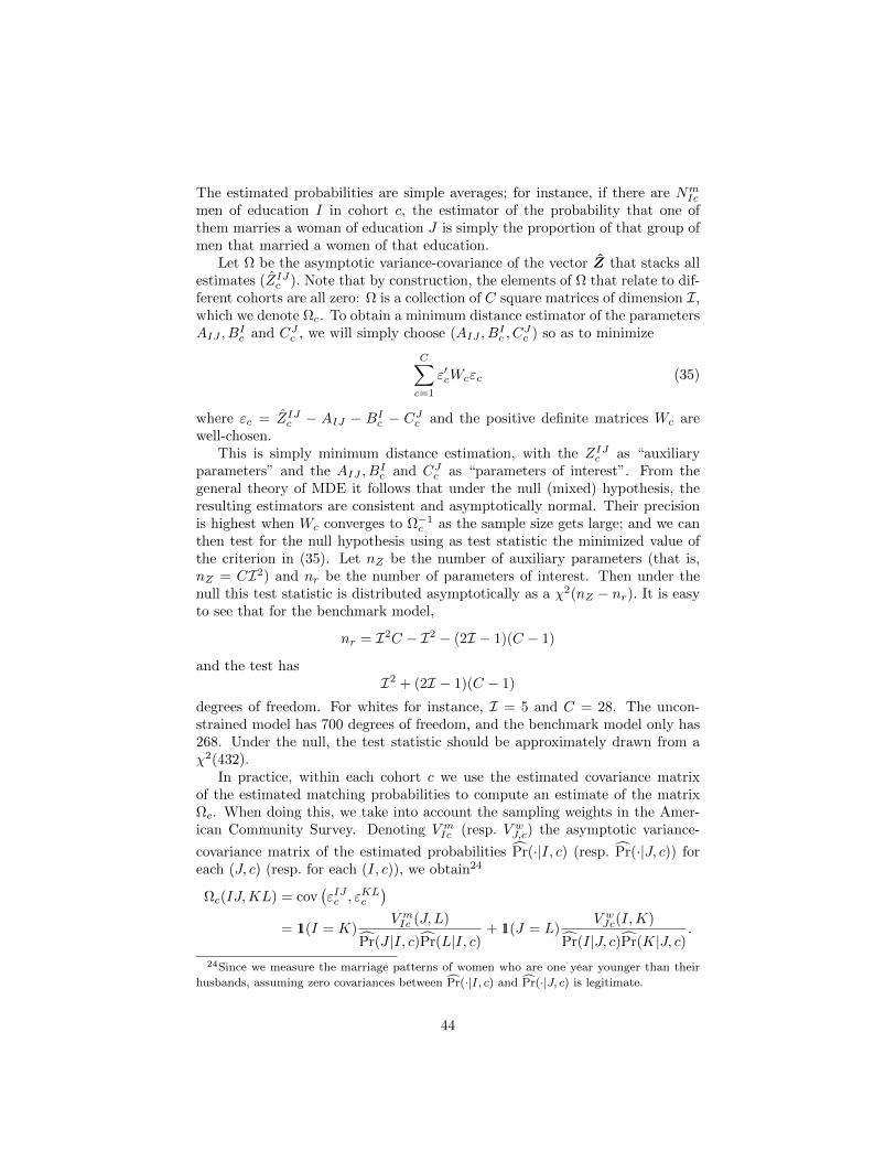
The estimated probabilities are simple averages; for instance, if there are NmIc

men of education I in cohort c, the estimator of the probability that one ofthem marries a woman of education J is simply the proportion of that group ofmen that married a women of that education.

Let Ω be the asymptotic variance-covariance of the vector Z that stacks allestimates (ZIJc ). Note that by construction, the elements of Ω that relate to dif-ferent cohorts are all zero: Ω is a collection of C square matrices of dimension I,which we denote Ωc. To obtain a minimum distance estimator of the parametersAIJ , B

Ic and CJc , we will simply choose (AIJ , B

Ic , C

Jc ) so as to minimize

C∑c=1

ε′cWcεc (35)

where εc = ZIJc − AIJ − BIc − CJc and the positive definite matrices Wc arewell-chosen.

This is simply minimum distance estimation, with the ZIJc as “auxiliaryparameters” and the AIJ , B

Ic and CJc as “parameters of interest”. From the

general theory of MDE it follows that under the null (mixed) hypothesis, theresulting estimators are consistent and asymptotically normal. Their precisionis highest when Wc converges to Ω−1c as the sample size gets large; and we canthen test for the null hypothesis using as test statistic the minimized value ofthe criterion in (35). Let nZ be the number of auxiliary parameters (that is,nZ = CI2) and nr be the number of parameters of interest. Then under thenull this test statistic is distributed asymptotically as a χ2(nZ − nr). It is easyto see that for the benchmark model,

nr = I2C − I2 − (2I − 1)(C − 1)

and the test hasI2 + (2I − 1)(C − 1)

degrees of freedom. For whites for instance, I = 5 and C = 28. The uncon-strained model has 700 degrees of freedom, and the benchmark model only has268. Under the null, the test statistic should be approximately drawn from aχ2(432).

In practice, within each cohort c we use the estimated covariance matrixof the estimated matching probabilities to compute an estimate of the matrixΩc. When doing this, we take into account the sampling weights in the Amer-ican Community Survey. Denoting V mIc (resp. V wJ,c) the asymptotic variance-

covariance matrix of the estimated probabilities Pr(·|I, c) (resp. Pr(·|J, c)) foreach (J, c) (resp. for each (I, c)), we obtain24

Ωc(IJ,KL) = cov(εIJc , εKLc

)= 11(I = K)

V mIc (J, L)

Pr(J |I, c)Pr(L|I, c)+ 11(J = L)

V wJc(I,K)

Pr(I|J, c)Pr(K|J, c).

24Since we measure the marriage patterns of women who are one year younger than their

husbands, assuming zero covariances between Pr(·|I, c) and Pr(·|J, c) is legitimate.

44

Minimizing the expression in (35) is very simple since the εc terms are linearin the unknown parameters. The only (minor) difficulty is to keep track of thenecessary location normalizations.

5.2 The extensions

5.2.1 Changing complementarities

The models with time-varying complementarities of section 4.2.1 can be dealtwith in exactly the same way, and so can the models with preferences for agedifferences of section 4.2.3. Only the numbers of degrees of freedom of the χ2

differ, because these extensions have more parameters, and because (for themodel with age differences) we fit more margins.

5.2.2 The Heteroskedastic Model

Introducing heteroskedasticity as in section 4.2.2 only complicates inferenceslightly. With time-invariant heteroskedasticity, our basic identity now is

ZcIJ = σI logPr(J |I, c)Pr(0|I, c)

+ µJ logPr(I|J, c)Pr(0|J, c)

.

First assume that complementarities are constant across cohorts. Then the nullhypothesis is:

(H0) : ∃(σI , µJ , AIJ , BIc , CJc ) s.t. σI log Pr(J |I, c)+µJ log Pr(I|J, c) = AIJ+BIc+CJc .

Note that this involves (2I − 1) additional parameters (we need to keep one ofthe σ, µ’s equal to one.)

The more important change is that the asymptotic covariance matrix Ωcnow involves the unknown parameters σI and µJ :

Ωc(IJ,KL) = Varasymp

(σI log Pr(J |I, c) + µJ log Pr(I|J, c)

).

We are especially interested in testing the null hypothesis of homoskedasticity(our Choo and Siow benchmark) within the broader hypothesis (H0). AlainMonfort and Roger Rabemananjara (1990) show that this can be done by simply

1. choosing Wc as we did for the benchmark model;

2. minimizingC∑c=1

ε′cWcεc

where this time εIJc = σI log Pr(J |I, c)+µJ log Pr(I|J, c)−AIJ −BIc −CJcand we minimize over the (σ, µ,A,B,C) parameters

3. and subtracting the value of this minimized criterion from that of theminimized benchmark criterion.

45

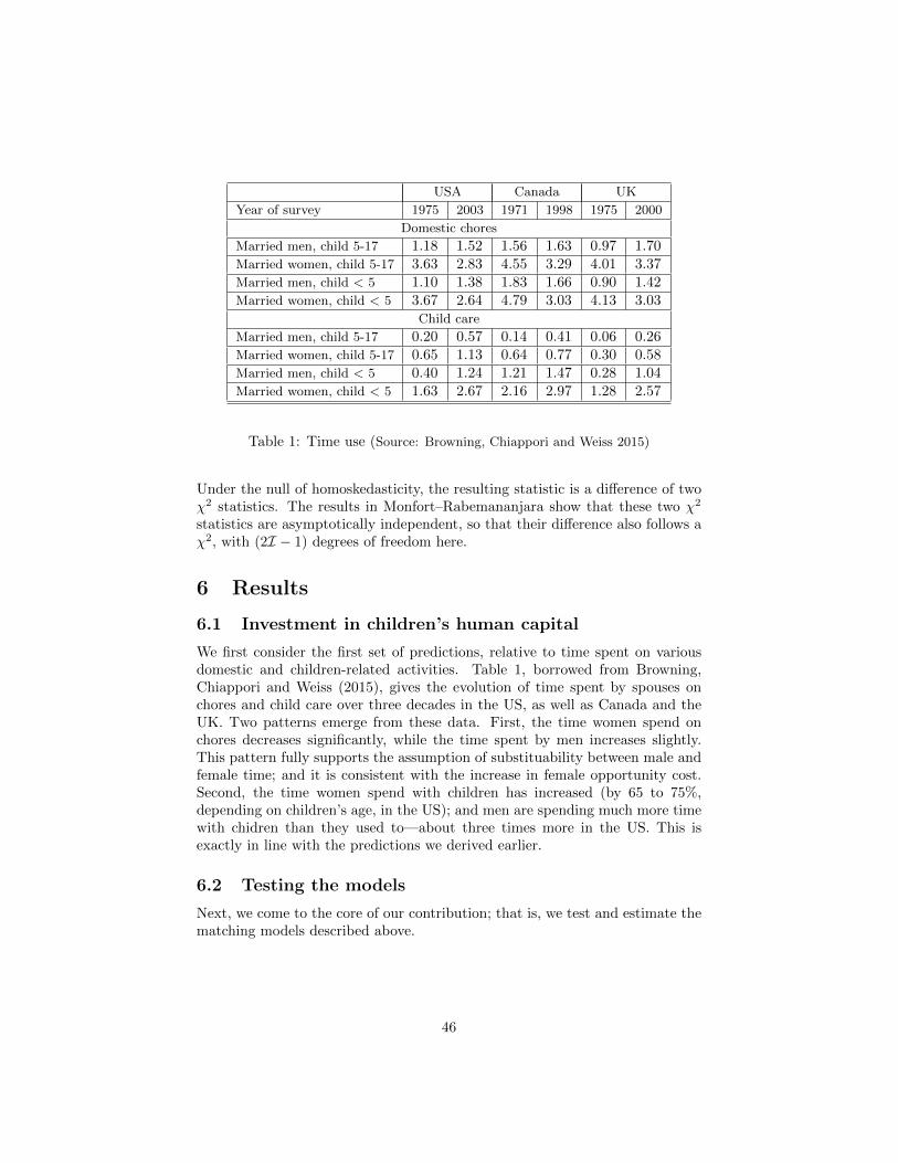
USA Canada UK

Year of survey 1975 2003 1971 1998 1975 2000

Domestic chores

Married men, child 5-17 1.18 1.52 1.56 1.63 0.97 1.70Married women, child 5-17 3.63 2.83 4.55 3.29 4.01 3.37Married men, child < 5 1.10 1.38 1.83 1.66 0.90 1.42Married women, child < 5 3.67 2.64 4.79 3.03 4.13 3.03

Child care

Married men, child 5-17 0.20 0.57 0.14 0.41 0.06 0.26Married women, child 5-17 0.65 1.13 0.64 0.77 0.30 0.58Married men, child < 5 0.40 1.24 1.21 1.47 0.28 1.04Married women, child < 5 1.63 2.67 2.16 2.97 1.28 2.57

Table 1: Time use (Source: Browning, Chiappori and Weiss 2015)

Under the null of homoskedasticity, the resulting statistic is a difference of twoχ2 statistics. The results in Monfort–Rabemananjara show that these two χ2

statistics are asymptotically independent, so that their difference also follows aχ2, with (2I − 1) degrees of freedom here.

6 Results

6.1 Investment in children’s human capital

We first consider the first set of predictions, relative to time spent on variousdomestic and children-related activities. Table 1, borrowed from Browning,Chiappori and Weiss (2015), gives the evolution of time spent by spouses onchores and child care over three decades in the US, as well as Canada and theUK. Two patterns emerge from these data. First, the time women spend onchores decreases significantly, while the time spent by men increases slightly.This pattern fully supports the assumption of substituability between male andfemale time; and it is consistent with the increase in female opportunity cost.Second, the time women spend with children has increased (by 65 to 75%,depending on children’s age, in the US); and men are spending much more timewith chidren than they used to—about three times more in the US. This isexactly in line with the predictions we derived earlier.

6.2 Testing the models

Next, we come to the core of our contribution; that is, we test and estimate thematching models described above.

46

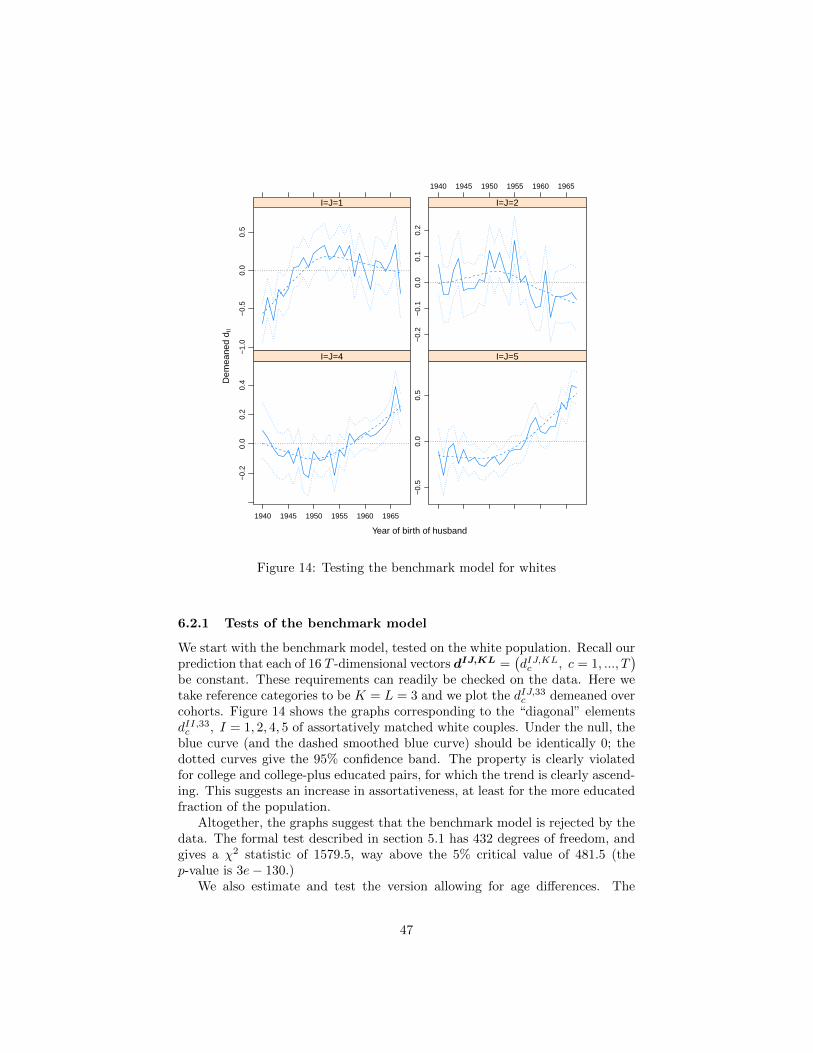
Year of birth of husband

Dem

eane

d d I

I

−1.

0−

0.5

0.0

0.5

I=J=1

1940 1945 1950 1955 1960 1965

−0.

2−

0.1

0.0

0.1

0.2

I=J=2

−0.

20.

00.

20.

4

1940 1945 1950 1955 1960 1965

I=J=4

−0.

50.

00.

5

I=J=5

Figure 14: Testing the benchmark model for whites

6.2.1 Tests of the benchmark model

We start with the benchmark model, tested on the white population. Recall ourprediction that each of 16 T -dimensional vectors dIJ,KL =

(dIJ,KLc , c = 1, ..., T

)be constant. These requirements can readily be checked on the data. Here wetake reference categories to be K = L = 3 and we plot the dIJ,33c demeaned overcohorts. Figure 14 shows the graphs corresponding to the “diagonal” elementsdII,33c , I = 1, 2, 4, 5 of assortatively matched white couples. Under the null, theblue curve (and the dashed smoothed blue curve) should be identically 0; thedotted curves give the 95% confidence band. The property is clearly violatedfor college and college-plus educated pairs, for which the trend is clearly ascend-ing. This suggests an increase in assortativeness, at least for the more educatedfraction of the population.

Altogether, the graphs suggest that the benchmark model is rejected by thedata. The formal test described in section 5.1 has 432 degrees of freedom, andgives a χ2 statistic of 1579.5, way above the 5% critical value of 481.5 (thep-value is 3e− 130.)

We also estimate and test the version allowing for age differences. The

47

conclusions are similar: when we average errors over age differences as discussedabove, the χ2 statistic has value 1526.5 with 405 degrees of freedom, whilethe 5% critical value is 452.9, leading to a p-value that the computer cannotdistinguish from 0.

Our findings are totally different for black couples. Given the much smallersample size, especially for higher education, we only use four education cate-gories, aggregating college and college-plus. Figure 15 shows little evidence fordeviations from the benchmark model. The formal test confirms this visual im-pression. The number of degrees of freedom is now 198, leading to a 5% criticalvalue of 231.8. The χ2 statistic is 174.9, which corresponds to a p-value of 0.88.We therefore fail to reject the null that preferences for assortativeness have notchanged over the period among the African-American population.

Our test of course has less power on a smaller sample; and there are twentytimes fewer black couples than white couples in our data. For any given devi-ation from the null hypothesis, the χ2 statistic is known to scale linearly withsample size. Multiplying the value of the χ2 statistic for black couples by 20would lead to a clear rejection of the null. However, the value of the χ2 statisticwe obtained in an earlier version of the paper with five rather than seven wavesof the ACS was actually larger. Figure 15 also shows no clear pattern of devia-tions over time, unlike Figure 14. This suggests to us that our result for blackcouples is not simply due to low power.

6.2.2 White sample: extensions

Since the benchmark model is rejected for the white population, we next considerthe linear and quadratic extensions. Figure 16 gives, again for diagonal pairs(I, I), the standardized residuals of three regressions of the dII,33c , correspondingrespectively to the benchmark model, the linear trend, and the quadratic trendextensions. Since the variance is normalized to be 1, theory would require theseresiduals to remain between -1.96 and 1.96 for 95% of observations. The lineartrend models appear to fit data significantly better than the benchmark. More-over, while the quadratic component further increases the fit, its contributionis much more incremental.

While the model is still rejected, the rejection is much less drastic thanpreviously. Specifically, the χ2 statistic is 676.7, while the 5% critical value (for416 degrees of freedom) is 464.6. The spectacular decrease in the χ2 statisticindicate that preferences did change over the period; an exact description ofthese changes is provided in the next subsection. Under the quadratic version,the number of degrees of freedom is now 400, giving a 5% critical value of 447.6;the test statistic equals 523.0. The null that all quadratic terms are zero isrejected. The test using age differences gives very similar results.

We therefore conclude that in the white population, the surplus generatedby assortativeness changed significantly over the period. The direction of thesechanges is quite interesting. Remember from section 4.2.1 that these changespush towards more assortativeness if and only if the matrix b formed by thecoefficients of the linear trends in (32) is supermodular, that is iff each DIJ,KLb

48

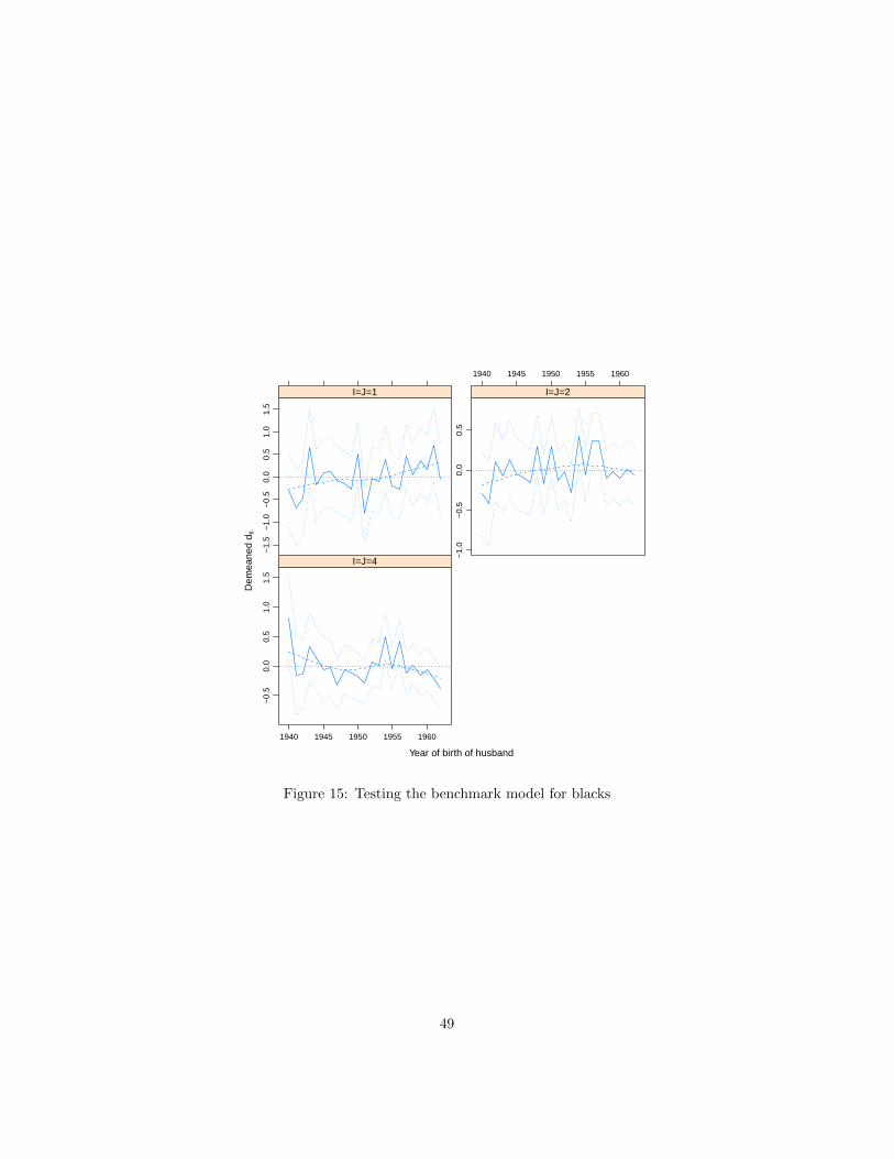
Year of birth of husband

Dem

eane

d d I

I

−1.

5−

1.0

−0.

50.

00.

51.

01.

5

I=J=1

1940 1945 1950 1955 1960

−1.

0−

0.5

0.0

0.5

I=J=2

−0.

50.

00.

51.

01.

5

1940 1945 1950 1955 1960

I=J=4

Figure 15: Testing the benchmark model for blacks

49

Year of birth of husband

Sta

ndar

dize

d er

rors −4

−2

02

I=J=1

1940 1950 1960−

2−

10

12

I=J=2

−2

−1

01

23

I=J=3

−4

−2

02

4

1940 1950 1960

I=J=4

−4

−2

02

4

I=J=5

Choo−SiowLinear trendsQuadratic trends

Figure 16: Testing various models for whites

50

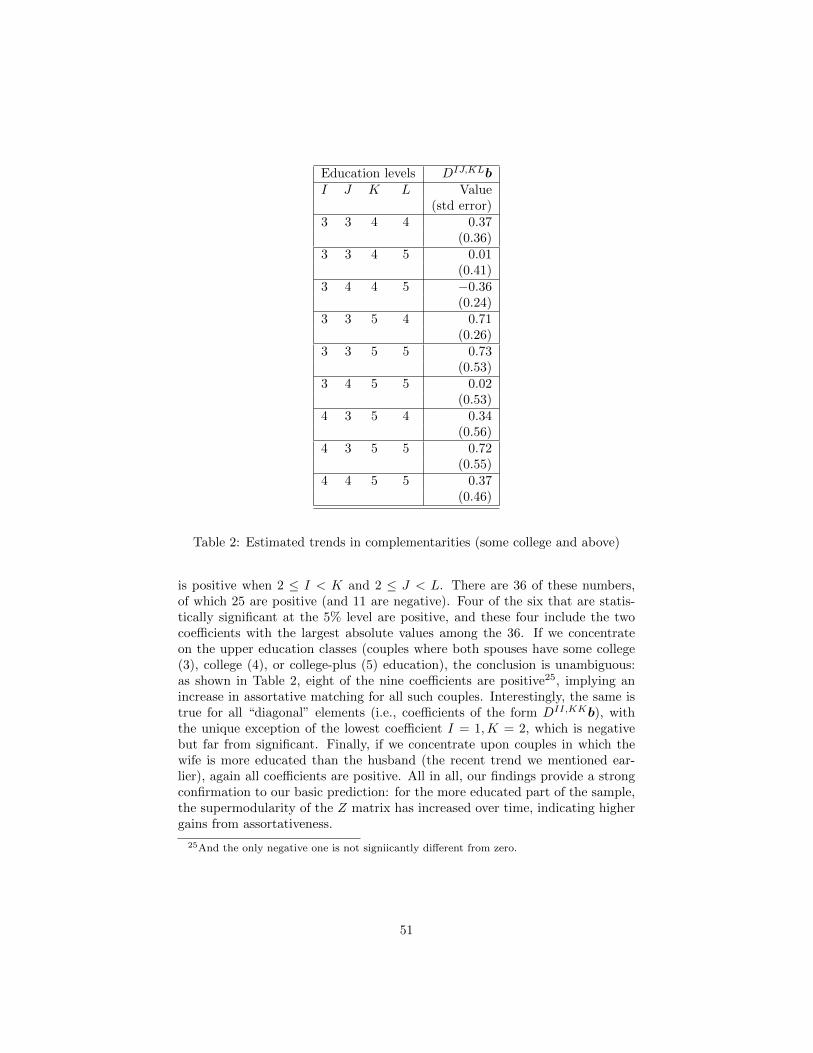
Education levels DIJ,KLbI J K L Value

(std error)3 3 4 4 0.37

(0.36)3 3 4 5 0.01

(0.41)3 4 4 5 −0.36

(0.24)3 3 5 4 0.71

(0.26)3 3 5 5 0.73

(0.53)3 4 5 5 0.02

(0.53)4 3 5 4 0.34

(0.56)4 3 5 5 0.72

(0.55)4 4 5 5 0.37

(0.46)

Table 2: Estimated trends in complementarities (some college and above)

is positive when 2 ≤ I < K and 2 ≤ J < L. There are 36 of these numbers,of which 25 are positive (and 11 are negative). Four of the six that are statis-tically significant at the 5% level are positive, and these four include the twocoefficients with the largest absolute values among the 36. If we concentrateon the upper education classes (couples where both spouses have some college(3), college (4), or college-plus (5) education), the conclusion is unambiguous:as shown in Table 2, eight of the nine coefficients are positive25, implying anincrease in assortative matching for all such couples. Interestingly, the same istrue for all “diagonal” elements (i.e., coefficients of the form DII,KKb), withthe unique exception of the lowest coefficient I = 1,K = 2, which is negativebut far from significant. Finally, if we concentrate upon couples in which thewife is more educated than the husband (the recent trend we mentioned ear-lier), again all coefficients are positive. All in all, our findings provide a strongconfirmation to our basic prediction: for the more educated part of the sample,the supermodularity of the Z matrix has increased over time, indicating highergains from assortativeness.

25And the only negative one is not signiicantly different from zero.

51

6.2.3 Heteroskedasticity

We next test for heteroskedasticity along the lines suggested in 4.2.2. Remem-ber that our test statistic is the difference of two χ2’s, one of which is computedover the best heteroskedastic model. Unfortunately, we haven’t been able toestimate a fully heteroskedastic model: some of the µJ ’s (the dispersion param-eters for women) go to the lower bound of zero. We settled on an approach inwhich we only allow the dispersions for one gender to deviate from the value ofone. These two semi-heteroskedastic models converged without difficulty. Theevidence for hetoroskedasticity is strong, with p-values smaller than 1e − 30for both genders. However, allowing for this semi-heteroskedasticity does notimprove the fit of the model much: the χ2 statistic only decreases from its “ho-moskedastic” value of 1579.5 to 1385 for the men-heteroskedastic and 1425 forthe women-heteroskedastic models. The data still spectacularly rejects modelswith constant complementarities.

A heteroskedastic model with time trands affecting the supermodular coreis in principle identifiable; but in practice the empirical estimates are not ro-bust, possibly indicating an overparametrization. Given our emphasis on theevolution of assortativeness across cohorts, we keep the trends but omit het-eroskedasticity in what follows.

6.3 The marital college premium: the African-Americansample

Since the benchmark model is not rejected for Afro-Americans, we can directlyanalyze its implications. Figure 17 shows the evolution of male and femaleexpected surplus by class of education. Two patterns emerge from this diagram.First, the marital surplus declines over the period, more strongly for men thanfor women. More importantly, however, there is no significant difference betweeneducation classes; for each gender, the decline is very similar across educationlevels. Fitting linear trends confirms the visual impression. The value of a high-school degree has a significant negative trend for both men and women, and thevalue of a college degree has a significant positive trend for women; but theyare very small, as Figure 17 suggests.

Therefore the “marital education premia”, defined as the difference in ex-pected marital surplus between education classes, stayed almost constant formen as well as for women. In particular, the additional marital expected utilityfrom a college degree hardly changed over the period for both men and women.

This finding can be related to the specific evolution of the demand for highereducation among African-Americans over the period: as discussed earlier, nosignificant difference appears between men and women. While a precise inves-tigation of the causes for that difference is beyond the scope of this paper, anatural suggestion is that it may be related to differences in attitudes and so-cial norms regarding children education. In a recent contribution, Gayle, Golanand Soytas (2014) show for instance that married black women spend muchless time with children than their white counterparts, despite little difference in

52

1940 1945 1950 1955 1960

0.0

0.5

1.0

1.5

2.0

Year of birth

u I

HSDHSGSC CG

1940 1945 1950 1955 1960

0.0

0.5

1.0

1.5

2.0

Year of birth

v J

HSDHSGSC CG

Figure 17: Expected utilities of black men and women

53

education level and a slightly larger number of children.26 This difference maybe caused by race-specific costs of education and differences in parental stylesbetween black and whites, as suggested by Neal (2006) in his extensive survey ofthe topic27; or it may reflect divergent perceptions of the benefits of education,as argued by several sociologists28. This remains an underinvestigated question.

6.4 The white population

6.4.1 The marital college premium: evolution over cohorts

The estimation of the structural model allows to compute the evolution of themarital college premium by gender over the cohorts under consideration. Fig-ure 18 represents our estimate of the expected utilities from marriage for menand women. Three facts stand out. First, these gains decrease over the period,for all genders and education levels. Second, the decrease is much stronger forlower levels of education. Thirdly, and more interestingly for our purpose, maleand female profiles are dissimilar.

The marital gains of men increase with education for all cohorts. Moreover,while the marital college premium increases over the period, the plots of mari-tal gains for the two highest levels of education—college and college-plus—arealmost parallel: the “college-plus premium”, defined as the difference in maritalutility between college and college-plus, remains constant over the period.

For women, however, the picture is radically different. For the older cohorts,the marital gain is inversely related to education (with the exception of highschool drop outs.) While marital gains trend downwards, the decrease is muchslower for educated individuals; as a result, the more recent cohorts exhibitmarital gains that are higher for college-educated women. Even more interestingis the spectacular reduction of the difference between college and college-pluswomen, which translates into a strong increase in the college-plus premium forwomen. As a result, the (double) difference between female and male maritalcollege-plus premia increases significantly over the period (see Figure 19, whichonly shows one-standard error confidence bands for legibility.)

Using the same notation as above, if uIc (resp. vIc ) denotes the expectedmarital gain for men (women) with education I in cohort c, we consider the

26“[. . . ] Married black females on average have slightly more children than married whitefemales (1.43 for blacks versus 1.27 for whites) but spend 30 percent less time with youngchildren than married white females. [. . . ] Thus in terms of demographic characteristics,black and white married females are similar but black married females spend less time withyoung children.” (Gayle et al 2015, p. 7).

27“[. . . ] there is some evidence that blacks attend less effective schools than white students,and although this racial gap in school quality cannot be linked to racial differences in schoolfunding levels, it may indicate that blacks pay higher implicit, if not explicit, costs to attendquality schools” (p. 562), and “[. . . ] the fact that parenting behaviors differ greatly byrace among families that are similar with respect to wealth, neighborhood quality, familystructure, and measured maternal human capital raises the possibility that norms concerningchild rearing differ among blacks and whites in important ways” (p. 568).

28See, for instance, the literature on “acting white”. Again, the reader is refered to Neal(2006) for a detailed discussion.

54

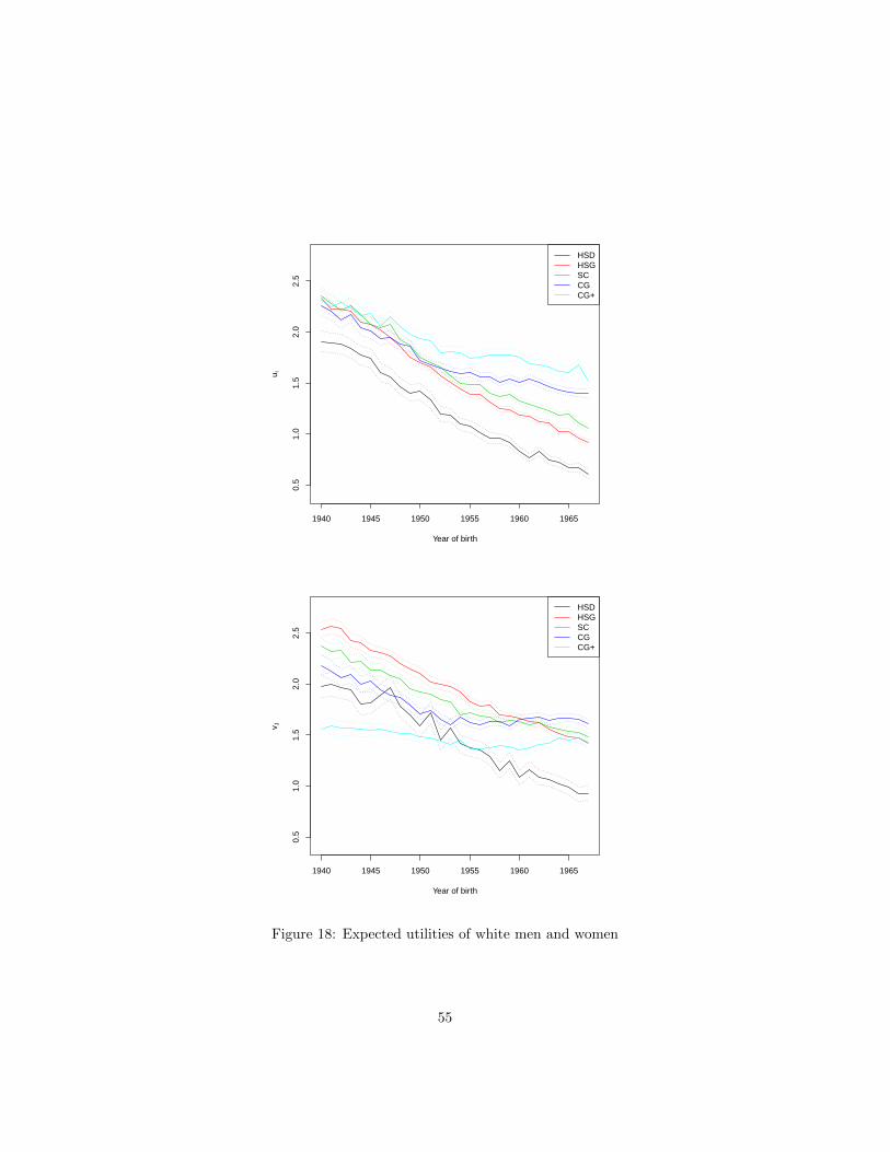
1940 1945 1950 1955 1960 1965

0.5

1.0

1.5

2.0

2.5

Year of birth

u I

HSDHSGSC CG CG+

1940 1945 1950 1955 1960 1965

0.5

1.0

1.5

2.0

2.5

Year of birth

v J

HSDHSGSC CG CG+

Figure 18: Expected utilities of white men and women

55

1940 1945 1950 1955 1960 1965

−0.

8−

0.6

−0.

4−

0.2

0.0

0.2

0.4

Birth year of the man

Util

ity d

oubl

e−di

ffere

nce

HSD −−> HSGHSG −−> SC SC −−> CG CG −−> CG+

Figure 19: Excess premia of white women

56

evolution of the double difference

δIc =(vI+1c − vIc

)−(uI+1c − uIc

)over cohorts. For I = 4 for instance, uI+1

c − uIc thus represents the college-pluspremium for men, and δIc is the difference in the college-plus premia of womenand men. When regressing our estimated δ4c on a linear time trend, we find apositive coefficient that is highly significant, both in statistical and economicterms. In contrast, the other δIc are either flat or (for I = 2, which is thetransition to “some college”) increase significantly but more slowly.

In summary, we see a significant increase in the college-plus premium forwomen, whereas no such evolution is apparent for men or for other educationaltransitions. It bears repeating that this conclusion obtains from the sole analysisof matching patterns over time, without any other data on intrahousehold al-locations. It nevertheless strongly supports CIW’s suggestion that the increasein female demand for higher education could be motivated in part by the diver-gences between the respective evolutions of male and female marital college-pluspremia.29

6.4.2 Decomposition

The marital college premium can be decomposed into several components. First,education affects the probability of being married. Second, conditional on beingmarried, it also affects the education of the spouse (or more exactly its prob-ability distribution); intuitively, we expect educated women to find a “better”husband, at least in terms of education, and conversely. Third, the impact onthe total surplus generated by marriage is twofold. Take women for instance.A wife’s education has a direct impact on the surplus; this impact can be mea-sured, for college-plus education, by the difference (ZI5c −ZI4c ). In addition, sincea more educated woman is more likely to marry a more educated husband, thehusband’s higher expected education further boosts the surplus, by the averageof the (Z5J

c − Z4Jc ) terms weighted by the difference in probability of marry-

ing a college-plus educated husband instead of a college graduate. Finally, theshare of the surplus going to the wife in any given match is also affected by hereducation. This share is given by the ratio

vJcuIc + vJc

for a woman of education J who marries a man of education I.All these components are readily computed from our estimates; they are

summarized in Tables 3 to 7. The first three tables summarize patterns that we

29As noted before, a limitation of our analysis is the lack of adequate data on divorce. Thestudy by Schwartz and Han (2014) reports that for recent cohorts, being more educated thanthe husband is no longer a handicap for women in terms of divorce probability. Althoughbased on very small samples, this finding is consistent with the rising incentive of women toinvest in schooling that our model predicts.

57

already discussed in the introduction. The marriage probabilities decline, verysharply for less educated individuals, and much less for college-educated womenespecially. Educated men are more likely to marry an educated wife than theyused to. The pattern is opposite for college-educated women; in partiuclar theyare much less likely to marry a college-plus husband.

More interesting are the last two tables, which are specific to our structuralapproach. The joint surplus declines in 17 of the 25 cells. Of the eight positivecells (in bold in Table 6), seven concern couples formed by college or college-plus educated women; and in all of these eight cells, the wife is at least aseducated as the husband. The decline in surplus is always smaller (or inverted)for more educated couples, which is consistent with the increased preferences forassortativeness at the top of the distribution. Lastly, the intra-household dis-tribution of the surplus also varies significantly. The share of the wife increasesfor matches between equally educated individuals. Things are more complex offthe diagonal. The share received by educated women who marry down tendsto decrease (see the cells above the diagonal in Table 7). On the other hand,less educated women who marry up benefit from a significantly larger share ofa joint surplus which has become smaller over the years.

Conclusion

It has long been recognized (at least since Becker’s 1973 seminal contributions)that the division of the surplus generated by marriage should be analyzed asan equilibrium phenomenon. As such, it responds to changes in the economicenvironment; conversely, investments made before marriage are partly driven byagents’ current expectations about the division of surplus that will prevail aftermarriage. Theory shows that such considerations may explain the considerabledifferences in male and female demands for higher education. When decidingwhether to go to college, agents take into account not only the labor marketcollege premium (i.e., the wage differential resulting from a college education)but also the “marital college premium” , which represents the impact of edu-cation on marital prospects; the latter includes not only marriage probabilities,but also the expected “quality” of the future spouse and the resulting size anddistribution of the marital surplus. While the first aspect—the labor marketcollege premium—has been abundantly discussed, the second—the marital col-lege premium—has been all but ignored. We argued in this paper that thisomission may have severely hampered our understanding of recent evolutions inthe demand for higher education.

We provided a simple but rich model in which the marital college premiumcan be econometrically identified. Our framework generalizes the original contri-bution by Choo and Siow (2006); it can be (over)identified using temporal vari-ations in the compositions of the populations. Applying the model to US data,we find gender- and race-specific evolutions. There is no evidence of changesin preference for assortativeness among the black population; among whites,on the contrary, we find a highly significant increase, particularly among the

58

most educated subsample. The evolution of the marital college and college-pluspremium is similar across genders for the African-American population; thissharply contrasts with the white sample, where the marital college-plus pre-mium increases much more for women that for men. All in all, our findingssupport the claim that the marriage market has played an important role in thedemand for higher education in the recent decades.

We claim that these evolutions can be explained by basic economic argu-ments. The value of investment in children’s human capital has drasticallyincreased over the period, while the amount of time available was boosted bytechnological innovations that freed households—i.e., at that period, mostlywomen—from spending huge amount of time on basic chores. A first conse-quence has been a drastic change in time allocation patterns: less time wasspent on chores and much more on children. As theory predicts, these shiftshave resulted in significant changes in matching patterns. They can explain inparticular the significant increase in assortative matching that several authorsobserved—and that our more structural estimation confirms—at the top of thehuman capital distribution. This impact was amplified by the self-reinforcingnature of the equilibrium. An initial impulse affecting a gender’s stock of hu-man capital, added to a slight difference in initial ability (as described by GaryBecker, William Hubbard and Kevin Murphy 2010) results in higher incentivesto invest in education, and ultimately in significant changes in both educationprofiles and marital patterns.

All in all, what we have seen operating is a boost in returns to human capitalinvestments, resulting not only in higher incentives to invest, but in a generalreshuffling of equilibrium patterns on the marriage market. Our belief is thatexplicit modelling can help shed light on these complex mechanisms.

59

Men WomenEarly Late Change Early Late Change

HS Dropouts 0.85 0.48 -0.37 0.86 0.61 -0.25HS Graduates 0.90 0.62 -0.27 0.92 0.77 -0.15Some College 0.90 0.67 -0.22 0.90 0.78 -0.12College 0.89 0.75 -0.13 0.88 0.81 -0.07College-plus 0.90 0.80 -0.10 0.79 0.77 -0.03

Table 3: Probabilities of marriage

Wife → HSD HSG SC CG CG+Early Cohorts

HSD 0.37 0.47 0.14 0.02 0.01HSG 0.09 0.65 0.20 0.04 0.02SC 0.05 0.41 0.41 0.09 0.05CG 0.01 0.21 0.33 0.32 0.13CG+ 0.01 0.10 0.24 0.34 0.32

Late CohortsHSD 0.29 0.39 0.26 0.05 0.02HSG 0.04 0.46 0.33 0.12 0.04SC 0.01 0.20 0.46 0.23 0.09CG 0.00 0.07 0.21 0.52 0.20CG+ 0.00 0.03 0.12 0.42 0.42

ChangeHSD -0.08 -0.08 0.12 0.03 0.01HSG -0.05 -0.18 0.13 0.08 0.02SC -0.03 -0.21 0.06 0.14 0.04CG -0.01 -0.14 -0.12 0.20 0.07CG+ -0.00 -0.07 -0.11 0.08 0.11

Table 4: Partners of men

60

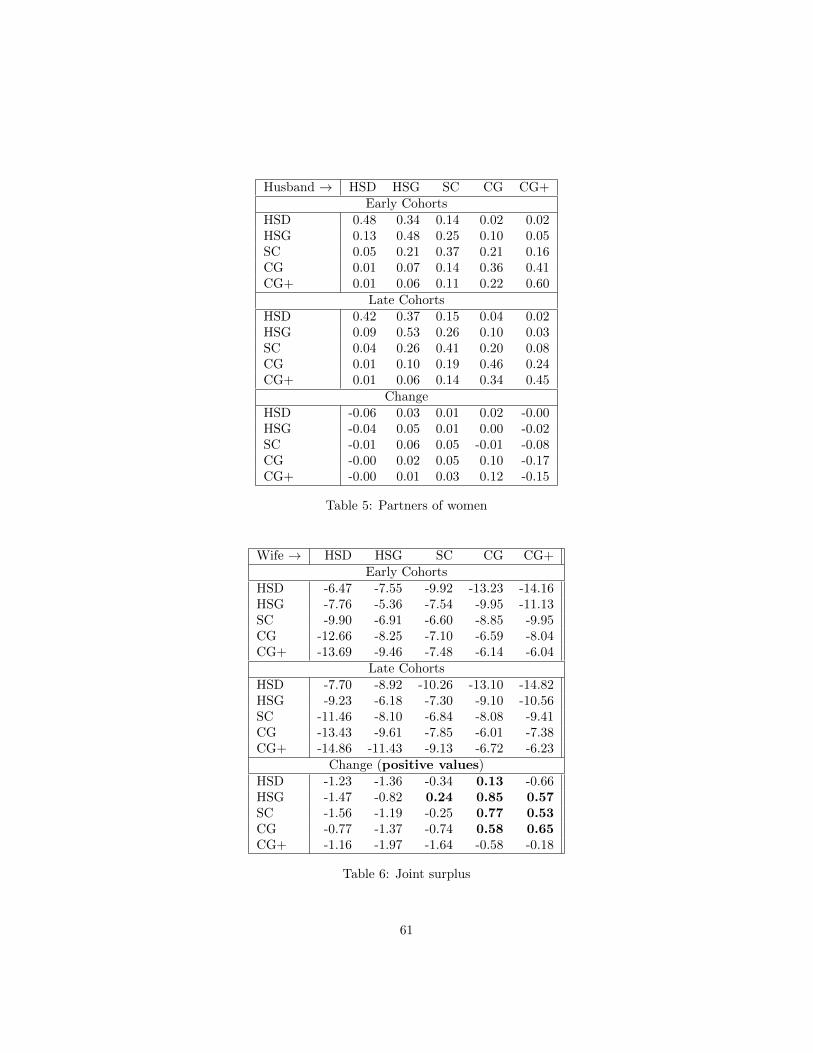
Husband → HSD HSG SC CG CG+Early Cohorts

HSD 0.48 0.34 0.14 0.02 0.02HSG 0.13 0.48 0.25 0.10 0.05SC 0.05 0.21 0.37 0.21 0.16CG 0.01 0.07 0.14 0.36 0.41CG+ 0.01 0.06 0.11 0.22 0.60

Late CohortsHSD 0.42 0.37 0.15 0.04 0.02HSG 0.09 0.53 0.26 0.10 0.03SC 0.04 0.26 0.41 0.20 0.08CG 0.01 0.10 0.19 0.46 0.24CG+ 0.01 0.06 0.14 0.34 0.45

ChangeHSD -0.06 0.03 0.01 0.02 -0.00HSG -0.04 0.05 0.01 0.00 -0.02SC -0.01 0.06 0.05 -0.01 -0.08CG -0.00 0.02 0.05 0.10 -0.17CG+ -0.00 0.01 0.03 0.12 -0.15

Table 5: Partners of women

Wife → HSD HSG SC CG CG+Early Cohorts

HSD -6.47 -7.55 -9.92 -13.23 -14.16HSG -7.76 -5.36 -7.54 -9.95 -11.13SC -9.90 -6.91 -6.60 -8.85 -9.95CG -12.66 -8.25 -7.10 -6.59 -8.04CG+ -13.69 -9.46 -7.48 -6.14 -6.04

Late CohortsHSD -7.70 -8.92 -10.26 -13.10 -14.82HSG -9.23 -6.18 -7.30 -9.10 -10.56SC -11.46 -8.10 -6.84 -8.08 -9.41CG -13.43 -9.61 -7.85 -6.01 -7.38CG+ -14.86 -11.43 -9.13 -6.72 -6.23

Change (positive values)HSD -1.23 -1.36 -0.34 0.13 -0.66HSG -1.47 -0.82 0.24 0.85 0.57SC -1.56 -1.19 -0.25 0.77 0.53CG -0.77 -1.37 -0.74 0.58 0.65CG+ -1.16 -1.97 -1.64 -0.58 -0.18

Table 6: Joint surplus

61

Wife → HSD HSG SC CG CG+Early Cohorts

HSD 0.51 0.45 0.47 0.49 0.57HSG 0.60 0.53 0.55 0.58 0.66SC 0.55 0.48 0.51 0.53 0.61CG 0.51 0.45 0.47 0.49 0.56CG+ 0.37 0.33 0.34 0.36 0.41

Late CohortsHSD 0.59 0.45 0.44 0.41 0.45HSG 0.76 0.60 0.59 0.56 0.60SC 0.73 0.59 0.57 0.55 0.59CG 0.70 0.58 0.56 0.54 0.58CG+ 0.57 0.47 0.47 0.45 0.48

ChangeHSD 0.08 0.00 -0.03 -0.08 -0.12HSG 0.16 0.07 0.03 -0.02 -0.06SC 0.18 0.10 0.07 0.02 -0.02CG 0.19 0.13 0.10 0.05 0.01CG+ 0.20 0.15 0.13 0.09 0.07

Table 7: Surplus share of wife

References

Albanesi, S. and C. Olivetti (2009), “Gender Roles and Medical Progress”,NBER WP 14873.

Autor, D. (2014), “Skills, education, and the rise of earnings inequalityamong the “other 99 percent””, Science, 344, 843–851.

Becker, G. (1973), “A Theory of Marriage: Part I”, Journal of PoliticalEconomy, 81, 813–846.

Becker, G. (1974), “A Theory of Marriage: Part II”, Journal of PoliticalEconomy, 82, S11–S26.

Becker, G. (1991), Treatise on the family, Cambridge Mass: HarvardUniversity Press.

Becker, Gary S., William H. J. Hubbard, and Kevin M. Murphy(2010), “The Market for College Graduates and the Worldwide Boom in HigherEducation of Women”, American Economic Review, 100(2): 229-33.

Bergstrom, T. and R. Cornes (1983), “Independence of Allocative Ef-ficiency from Distribution in the Theory of Public Goods”, Econometrica, 51,1753–1765.

Botticini, M., and A. Siow (2008), “Are there Increasing Returns inMarriage Markets?”, University of Toronto, mimeo.

Bronson, M. A. (2014), “Degrees Are Forever: Marriage, Educational

62

Investment, and Lifecycle Labor Decisions of Men and Women”, working paper,UCLA.

Browning, M., P.-A. Chiappori, and Y. Weiss (2014), Economics ofthe Family. Cambridge University Press, New York.

Bruze, G., Svarer M. and Y. Weiss (2015), “The Dynamics of Marriageand Divorce” , Journal of Labor Economics, 33, 123-170.

Chiappori, PA, and B. Salanie (2015), “The Econometrics of MatchingModels”, Journal of Economic Literature, forthcoming.

Chiappori, PA, M. Iyigun and Y. Weiss (2009), “Investment in School-ing and the Marriage Market” , American Economic Review, 99, 1689-1714.

Cherlin, A. (1992) Marriage, Divorce, Remarriage, Cambridge Mass:Harvard University Press.

Choo, E. and A. Siow (2006), “Who Marries Whom and Why” , Journalof Political Economy, 114, 175-201.

Dagsvik, J.K. (2000), “Aggregation in Matching Markets” InternationalEconomic Review, 41, 27–57.

Del Boca, Daniela, Christopher Flinn and Matthew Wiswall, 2014.“Transfers to Households with Children and Child Development,” IZA Discus-sion Paper 8393.

Doepke, M. and M. Tertilt (2009), “Womens Liberation: Whats in Itfor Men?”, Quarterly Journal of Economics, 124, 1541–91.

Doepke, M., M. Tertilt and A. Voena (2011), “The Economics andPolitics of Womens Rights”, NBER Working Paper 17672.

Fox, J. (2010a), “Identification in Matching Games”, Quantitative Eco-nomics, 1, 203–254.

Fox, J. (2016), “Estimating matching games with transfers”, Rice Univer-sity mimeo.

Fox, J., D. Hsu and C. Yang (2015), “Unobserved Heterogeneity inMatching Games with an Application to Venture Capital”, University of Michi-gan mimeo.

Galichon, A., and B. Salanie (2015), “Cupid’s Invisible Hand: SocialSurplus and Identification in Matching Models”, Columbia University mimeo.

Goldin, C. and Katz, L. (2002), “The power of the pill: oral con-traceptives and women’s career and marriage decisions” , Journal of PoliticalEconomy, 110, 730-770.

Goldin, C. and Katz, L. (2008), The Race Between Education AndTechnology, Harvard University Press, Cambridge.

Goldin, Claudia and Lawrence F. Katz (2009), ‘The Future of Inequal-ity: The Other Reason Education Matters So Much’, Aspen Institute Congres-sional Program 24(4): 7-14. Education Reform: Sixteenth Conference, August17-August 22, 2009. Washington, DC: Aspen Institute. Previously published inMilken Institute Review, 3rd Q 2009.

Graham, B. (2011), “Econometric Methods for the Analysis of Assign-ment Problems in the Presence of Complementarity and Social Spillovers” ,in J. Benhabib, M. Jackson and A. Bisin eds: Handbook of Social Economics,North-Holland, Vol. 1B, 965–1052.

63

Greenwood, J., A. Seshadri and M. Yorukoglu (2005), “Engines ofLiberation,” Review of Economic Studies, 72, 109–133.

Gullickson, A. (2006), “Black/White Interracial Marriage Trends, 1850-2000”, Journal of Family History, 32, 289-312.

Lundberg, S. and R.Pollak (2013), “Cohabitation and the Uneven Re-treat from Marriage in the U.S., 1950-2010”, NBER Working Paper 19413.

McFadden, D., (1973), “Conditional Logit Analysis of Qualitative ChoiceBehavior,” in P. Zarembka (ed.), Frontiers in Econometrics, 105-142, AcademicPress: New York.

Michael, R., (2000), “Abortion decisions in the U.S” , in Laumann, E,Michael, R (eds.), Sex, Love and Health: Public and Private Policy, Universityof Chicago Press.

Mishel, L., J. Bivens, E. Gould and H. Shierholz (2012), The Stateof Working America, 12th Edition, Cornell University Press, Ithaca.

Monfort, A. and and R. Rabemananjara (1990), “From a Var Modelto a Structural Model, with an Application to the Wage-Price Spiral”, Journalof Applied Econometrics, 5, 203–227.

Mourifie, I. and A. Siow (2014), “Cohabitation versus marriage: Mar-riage matching with peer effects”, University of Toronto mimeo.

Neal, D. and A. Rick (2014), “The Prison Boom and the Lack of BlackProgress After Smith and Welch”, NBER Working Paper 20283.

Ruggles, S., K. Genadek, R. Goeken, J. Grover, and M. Sobek(2015), “Integrated Public Use Microdata Series: Version 6.0 [Machine-readabledatabase]”. Minneapolis: University of Minnesota.

Schoen, R. and J. Klugel (1988), “The Widening Gap in Black andWhite Marriage Propensities”, American Sociological Review, 53, 895–907.

Schwartz, C. and Han, H. (2014) “The Reversal of the Gender Gap inEducation and Trends in Marital Dissolution ” Demography, 42, 621–646.

Schwartz, C. and Mare, R. (2005), “Trends in Educational AssortativeMarriage from 1940 to 2003” , American Sociological Review, 79, 605–629.

Shapley, L. and M. Shubik (1972), “The Assignment Game I: The Core”, International Journal of Game Theory, 1, 111–130.

Siow, A. (2009), “Testing Becker’s Theory of Positive Assortative Match-ing”, Discussion paper, University of Toronto.

Siow, A., and E. Choo (2006), “Estimating a Marriage Matching Modelwith Spillover Effects, ” Demography, 43, 463-490.

Seitz, S. (2009), “Accounting for Racial Differences in Marriage and Em-ployment,” Journal of Labor Economics, 27, 385-437.

Stevenson, B. and J. Wolfers (2007), “Marriage and Divorce: Changesand their Driving Forces”, Journal of Economic Perspectives, 21, 27–52.

Weiss, Y. and R. Willis (1997), “Match Quality, New Information, andMarital Dissolution” , Journal of Labor Economics, 15, 293-329.

Wilson, W. J., and K. Neckerman (1986), “Poverty and family struc-ture: The widening gap between evidence and public policy issues”, in S. H.Danziger & D. H. Wienberg (Eds.), Fighting poverty: What works and whatdoesn’t, Cambridge, MA: Harvard University Press.

64

Appendix A: Proof of Proposition 2

The proof is in several steps. Let (i ∈ I, j ∈ J) be a matched couple. Then:

1. First, man i must better off than being single, which gives:

U IJ + αIJi − αI∅i ≥ 0

hence αIJi − αI∅i ≥ −U IJ and the same must hold with woman j.

2. Take some woman j′ in J , currently married to some i′ in I. Then i mustbe better off matched with j than j′, which gives:

U IJ +(αIJi − αI∅i

)≥ zij′ − vj′

= ZIJ +(αIJi − αI∅i

)+(βIJj − β

∅Jj

)−(V IJ +

(βIJj′ − β

∅Jj′

))and one can readily check that this inequality is always satisfied as anequality, reflecting the fact that i is indifferent between j and j′, andsymmetrically j is indifferent between i and i′.

3. Take some woman k in K 6= J , currently married to some i′ in I. Then“i is better off matched with j than k” gives:

U IJ+(αIJi − αI∅i

)≥ zik−vk = ZIK+

(αIJi − αI∅i

)+βIKk −

(V IK + βIKk

)which is equivalent to

αIJi − αIKi ≥ U IK − U IJ

and we have proved that the conditions (18) are necessary. The proof isidentical for (19).

4. We now show that these conditions are sufficient. Assume, indeed, thatthey are satisfied. We want to show two properties. First, take somewoman j′ in J , currently married to some l in L 6= I. Then i is better offmatched with j than j′. Indeed,

U IJ +(αIJi − αI∅i

)≥ zij′ − vj′

= ZIJ +(αIJi − αI∅i

)+(βIJj − β

∅Jj

)−(V IJ +

(βIJj′ − β

∅Jj′

))is a direct consequence of (19) applied to l. Finally, take some womank in K 6= J , currently married to some l in L 6= I. Then i is better offmatched with j than j′. Indeed, it is sufficient to show that

U IJ + αIJi ≥ zik − vk = ZIK +(αIJi − αI∅i

)+ βIKk −

(V IK + βIKk

)

65

But from (19) applied to k we have that:

βLKk − βIKk ≥ V IK − V LK

and from (18) applied to i:

αIJi − αIKi ≥ U IK − U IJ

and the required inequality is just the sum of the previous two.

66