Universidad T´ ecnica Federico Santa Mar´ ıa. Departamento de F´ ısica. Particle Phenomenology in Spacetimes with Torsion Crist´obalCorral Advisor: Dr. Sergey Kovalenko Co-advisor: Dr. Oscar Castillo-Felisola A thesis submitted in partial fulfillment for the degree of Doctor in Science, Universidad T´ ecnica Federico Santa Mar´ ıa. March 2015

Welcome message from author
This document is posted to help you gain knowledge. Please leave a comment to let me know what you think about it! Share it to your friends and learn new things together.
Transcript
Universidad Tecnica Federico Santa Marıa.Departamento de Fısica.
Particle Phenomenology in Spacetimeswith Torsion
Cristobal CorralAdvisor: Dr. Sergey Kovalenko
Co-advisor: Dr. Oscar Castillo-Felisola
A thesis submitted in partial fulfillment for the degree of Doctorin Science, Universidad Tecnica Federico Santa Marıa.
March 2015

THESIS TITLE:
Particle Phenomenology in Spacetimes with Torsion
AUTHOR:
Cristobal Corral
A thesis submitted in partial fulfillment for the degree of Doctorin Science, Universidad Tecnica Federico Santa Marıa.
EXAMINATION COMMITTEE:
Dr. Sergey Kovalenko (UTFSM) . . . . . . . . . . . . . . . . . . . . . . . . . . . . . . . . . . . . . . . . .
Dr. Oscar Castillo-Felisola (UTFSM) . . . . . . . . . . . . . . . . . . . . . . . . . . . . . . . . . . . . . . . . .
Dr. Ivan Schmidt (UTFSM) . . . . . . . . . . . . . . . . . . . . . . . . . . . . . . . . . . . . . . . . .
Dr. Alfonso R. Zerwekh (UTFSM) . . . . . . . . . . . . . . . . . . . . . . . . . . . . . . . . . . . . . . . . .
Dr. Jorge Zanelli (CECs) . . . . . . . . . . . . . . . . . . . . . . . . . . . . . . . . . . . . . . . . .
March 19, 2015
Cristobal Corral i
to my wife Tania.
ii
This work is licensed under a Creative Commons Attribution-ShareAlike 4.0 InternationalLicense
Cristobal Corral iii

iv
Abstract
One of the natural extensions of the Riemannian geometry, was developed by Elie Cartanand it is known nowadays as the Riemann-Cartan geometry. Such an extension appears rathernaturally in the Poincare gauge theories (PGT) of gravitation and considers a nonvanishingtorsion into the picture. In vacuum, the introduction of torsion has no effect and gives thesame description as 4-dimensional General Relativity. However, the torsionful and torsion-freedescription of gravity are no longer equivalent in presence of certain matter fields. Particularly,the presence of fermions is rather interesting because its spin density acts as source of the torsionand, as a consequence, both theories differ by the presence of a four-fermion interaction, as soonas the torsion is integrated out. The aim of this thesis is to explore the phenomenological impactthat the inclusion of torsion might produce. For instance, we have found constraints on thefundamental Planck scale within extra dimensional models, by analyzing the torsion inducedfour-fermion interaction and the LHC data. Additionally, such an interaction induces correctionsto the one-loop observables within the Standard Model (SM) of particle physics, which was usedto obtain more stringent constraints on the fundamental Planck scale through the SM precisionmeasurements. Further, it was argued that the Yukawa sector of the SM may arise from thecondensation of a fourth family of heavy quarks, through the four-fermion interaction in gravitywith torsion. This approach gives rise to a composite Higgs boson. Finally, we considered twodifferent scenarios of torsion-descended axions and demonstrated that they are equivalent fromthe effective theory point of view. We studied the solution to the strong CP problem using suchkind of torsion-descended axions and examined some of their cosmological implications.
Cristobal Corral v

vi
Aknowledgements
First of all, I would like to appreciate all the love, patience and comprehensiveness of my wifeTania, who has been my support along my PhD studies. Without your disinterested way of love,your care and your unconditional help, this thesis would have not been possible. It is my pleasureto walk our life together. I love you.
During my whole career, I have received the infinite love, support and confidence of my parentsJorge and Gilda, my sister Catalina and my two brothers Jorge and Alejandro. They have believedin my life project of being a scientist. The person who I am now is due to their values, love andeducation. I love you all. Additionally, I feel extremely grateful about the homely reception andlove of my mother and father in law, Ema and Pedro, who have shared with me the pleasure ofbeing part of their beautiful family. Thank you both.
Along my PhD studies, I have counted with all the support and kindness of my advisor, Dr.Sergey Kovalenko, who has been an illuminating academic guidance during the completion ofmy PhD studies. He has shared with me, not only his wisdom and experience about physics,but how to manage the administrative issues as well. I really appreciate your personal advicesand dedication within the present thesis. Thank you very much. Additionally, I am infinitely in-debted with my colleague and personal friend, Dr. Oscar Castillo-Felisola, who has been a ratherimportant guide throughout my studies. For all your goodwill, wisdom and your insustituiblepersonal support along these years, thank you very much panita.
I really appreciate the gentleness and amiability of Dr. Ivan Schmidt, Dr. Alfonso Zerwekhand Dr. Jorge Zanelli, for being part of the committee of the present thesis. Thank you so muchfor your corrections, comments and feedback about the present work.
The essential part of my academic formation I owe to my professors at Universidad TecnicaFederico Santa Marıa (UTFSM) and Pontificia Universidad Catolica de Valparaıso (PUCV) whomI do not have the means to appreciate it enough. To Dr. Claudio Dib, Dr. Patricio Vargas, Dr.Olivier Espinosa (R.I.P.), Dr. Rene Rojas, Dr. Monica Pacheco, Dr. Miguel Calvo, amongothers, for their fabulous lectures. To Dr. Gorazd Cvetic and Dr. Patricio Haberle for theirrecommendation letters and advices when I asked them. To Dr. Carlos Contreras, Dr. PatricioGaete, Dr. Gonzalo Fuster for giving me the oportunity and confidence of working with themas an assistant. To professor Wladimir Ibanez for his dedication on teaching me some aspects ofexperimental physics, although I finished on the theoretical side. Thank you everyone.
To my friends and colleagues from UTFSM and PUCV, Felipe Rojas, Jilberto Zamora, Dr.Cesar Ayala, Dr. Adolfo Cisterna, Adolfo Toloza for your help, goodwill and advices about my
Cristobal Corral vii
work. To Bastian Dıaz, Gerardo Vasquez, Marcela Gonzalez, Nicolas Neill, Jorge Lopez, PedroAllendes, Gustavo Pulgar, Gonzalo Olavarrıa, Sebastian Tapia, Sebastian Ortiz, Rodrigo Valdes,Daniel Kroeger, Nelson Videla, Simon del Pino, Gaston Moreno, Dr. Juan Carlos Helo, Dr.Hayk Hakobyan, among others, for the fruitful discussions and kindness during my studies inValparaıso. Thanks.
I would like to thank the hospitality and kindness of Dr. Valery Lyubovitskij, Prof. Dr.Thomas Gutsche, Prof. Dr. Werner Vogelsang, Prof. Dr. Asmita Mukherjee, Prof. Dr. BarbaraJager, Dr. Wilco Den Dunnen, Dr. Marc Schlegel, Dr. Marco Strattman, Martin Lambert-sen, Jorg Schube, Astrid Hiller, Felix Ringer, Martin Schmidt, Daniele Anderle, Patriz Hinderer,Tom Kaufmann, Hannes Vogt, Markus Pak, Jan Heffer, Lukas Salfelder, Michael Benner, An-dreas Lange, Thomas Trauble, Peter Vastag, Demetrio Vilardi, Fabian Bohnet-Waldraff, MariusDommermuth, Ehsan Ebadati, Julien Fraisse, Muhammed Furkan Nur, Felix Hekhorn amongothers, from the Institut fur Theoretische Physik, Universitat Tubingen, Germany, during mystay there. To Stefanie Wahle-Hohloch for their hospitality, confidence, support and amiabilityfor receiving us in Tubingen during the whole 2014. Living in Germany has been one of the bestexperience of my life and you have made it worthwhile. Thanks a lot.
Finally, I am glad to thank to my personal friends with whom have spent several hours ofprofound conversations about life, politics and science. They have been like my family throughoutthese years far from my hometown. To Eduardo L., Pablo P.E., Eduardo B., Felipe A., CarlosQ., Javier B., Franco P., Adın A., Pablo P., Cristobal G., Constanza S., Camila L., Marıa JoseZ., Karen A., Lucas A., Jose Miguel B., Karina P., Marisol O., Marcia L. and Tamara L. all mygratitude for everything. To my friends from Santiago and La Serena, Elio C., Juan Jose M.,Andres B., Manuel P., Carolina H., Carolina F., Jorge M., Jose P., Mario F., Pablo P., ClaudioM., Manuel L., Jose G., Ignacio M., Gonzalo V., Diego V., Jose Pedro F., Jose Domingo G.,Fabrizio M., Juan M., Carla G., Cesar M. and all of them who have shared with me, thank youvery much.
The present thesis is supported by CONICYT, Chile, under the grant No. 21130179.
viii
Notation
Natural units ~ = 1 = c, where ~ is the reduced Planck constant while c is the speed of light.
Minkowski metric ηab = diag (−,+, . . . ,+).
Ψ and ψ stands for the D and the 4-dimensional Dirac spinors respectively. The Dirac adjointis denoted by Ψ = −ıΨ†γ0.
Spacetime (diffeomorphism) indices are denoted by greek letters i.e. µ, ν, λ, etc.
Tangent space (Lorentz) indices are denoted by latin letters, i.e. a, b, c, etc.
D-dimensional indices are denoted with a hat, i.e. µ, ν, and the 4-dimensional ones without ahat, i.e. µ, ν1.
Differential forms are denoted by bold symbols, i.e. ω = 1p! ωµ1...µp dx
µ1 ∧ . . . ∧ dxµp .
Antisymmetrization is denoted by square brackets, i.e. T[µ1...µp] = 1p!∑σ
(−1)|σ|Tσ(µ1)...σ(µp),where σ denotes permutation. For instance, M[µNν] = 1
2 (MµNν −MνNµ).
Multi-indices gamma matrices denotes antisymmetric product of them, i.e. γµ1...µp = γ[µ1 . . . γµp].For instance, γµν = 1
2 (γµγν − γνγµ).
Chiral gamma matrix γ∗ = (−ı)m+1 γ0γ1 . . . γD−1, where m stands for D = 2m.2 It satisfy(γ∗)2 = 1 and Tr γ∗ = 0.
The SU(N) indices are denoted by capital latin indices, i.e. A,B and so on, while the gener-ators are denoted by TA and satisfy the identities in Appendix B.
Ringed quantities denotes torsion-free ones, i.e. ωµab.
The antisymmetric symbol is normalized as ε01...D−1 = 1 = −ε01...D−1.
1However, throughout the first four chapters of this thesis, the hats over the indices are implicit. We will write it explicitly sincethe Chap. 5.
2In odd dimensions, the Clifford algebra is constructed with the gamma matrices in even dimensions plus the chiral gamma matrix.
Cristobal Corral ix

x
Contents
1 Introduction 1
2 Global Symmetries 5
2.1 What is a symmetry? . . . . . . . . . . . . . . . . . . . . . . . . . . . . . . . . . . 5
2.2 Internal global symmetry . . . . . . . . . . . . . . . . . . . . . . . . . . . . . . . . 6
2.3 Nother currents and conservation laws . . . . . . . . . . . . . . . . . . . . . . . . 6
2.4 Spacetime symmetries . . . . . . . . . . . . . . . . . . . . . . . . . . . . . . . . . 7
2.4.1 Lorentz transformations . . . . . . . . . . . . . . . . . . . . . . . . . . . . 7
2.4.2 Poincare transformations . . . . . . . . . . . . . . . . . . . . . . . . . . . . 9
3 Differential Geometry 11
3.1 Manifolds . . . . . . . . . . . . . . . . . . . . . . . . . . . . . . . . . . . . . . . . 11
3.2 Objects within the manifold . . . . . . . . . . . . . . . . . . . . . . . . . . . . . . 12
3.2.1 Scalars . . . . . . . . . . . . . . . . . . . . . . . . . . . . . . . . . . . . . . 12
3.2.2 Vectors . . . . . . . . . . . . . . . . . . . . . . . . . . . . . . . . . . . . . . 13
3.2.3 1-forms . . . . . . . . . . . . . . . . . . . . . . . . . . . . . . . . . . . . . 13
3.2.4 Tensors . . . . . . . . . . . . . . . . . . . . . . . . . . . . . . . . . . . . . 14
3.3 Lie derivative . . . . . . . . . . . . . . . . . . . . . . . . . . . . . . . . . . . . . . 14
3.4 Differential forms . . . . . . . . . . . . . . . . . . . . . . . . . . . . . . . . . . . . 15
Cristobal Corral xi
Contents
3.4.1 Wedge product . . . . . . . . . . . . . . . . . . . . . . . . . . . . . . . . . 16
3.4.2 Exterior derivative . . . . . . . . . . . . . . . . . . . . . . . . . . . . . . . 16
3.4.3 Interior product and Lie derivative . . . . . . . . . . . . . . . . . . . . . . 17
3.5 Covariant derivative and connections . . . . . . . . . . . . . . . . . . . . . . . . . 17
3.5.1 Parallel transport and geodesic . . . . . . . . . . . . . . . . . . . . . . . . 18
3.6 Riemannian and pseudo-Riemannian manifolds . . . . . . . . . . . . . . . . . . . . 19
3.6.1 The metric . . . . . . . . . . . . . . . . . . . . . . . . . . . . . . . . . . . 19
3.6.2 Metricity condition . . . . . . . . . . . . . . . . . . . . . . . . . . . . . . . 20
3.6.3 The vielbein . . . . . . . . . . . . . . . . . . . . . . . . . . . . . . . . . . . 20
3.6.4 Integration of differential forms . . . . . . . . . . . . . . . . . . . . . . . . 22
3.6.5 Hodge duality and inner product between forms . . . . . . . . . . . . . . . 23
3.7 Cartan’s structure equations . . . . . . . . . . . . . . . . . . . . . . . . . . . . . . 24
3.7.1 The first structure equation . . . . . . . . . . . . . . . . . . . . . . . . . . 24
3.7.2 Lorentz connection decomposition . . . . . . . . . . . . . . . . . . . . . . . 25
3.7.3 The second structure equation . . . . . . . . . . . . . . . . . . . . . . . . . 26
3.7.4 Bianchi identities . . . . . . . . . . . . . . . . . . . . . . . . . . . . . . . . 27
3.7.5 Relations between formalisms . . . . . . . . . . . . . . . . . . . . . . . . . 27
3.8 Actions in physics . . . . . . . . . . . . . . . . . . . . . . . . . . . . . . . . . . . . 28
3.8.1 The scalar field’s action . . . . . . . . . . . . . . . . . . . . . . . . . . . . 28
3.8.2 Abelian gauge field’s action . . . . . . . . . . . . . . . . . . . . . . . . . . 28
3.8.3 Non-Abelian gauge field’s action . . . . . . . . . . . . . . . . . . . . . . . . 29
3.8.4 Dirac field’s action . . . . . . . . . . . . . . . . . . . . . . . . . . . . . . . 29
3.8.5 Einstein-Cartan’s action . . . . . . . . . . . . . . . . . . . . . . . . . . . . 30
4 Gauge Symmetries 33
xii
4.1 Abelian gauge theory . . . . . . . . . . . . . . . . . . . . . . . . . . . . . . . . . . 33
4.2 Non-Abelian gauge symmetry: Yang-Mills theory . . . . . . . . . . . . . . . . . . 35
4.3 Local spacetime symmetries: Poincare Gauge Theory . . . . . . . . . . . . . . . . 36
5 Einstein-Cartan Theory 39
5.1 The vacuum case . . . . . . . . . . . . . . . . . . . . . . . . . . . . . . . . . . . . 39
5.2 Coupling scalars and vector fields . . . . . . . . . . . . . . . . . . . . . . . . . . . 40
5.3 Coupling fermions . . . . . . . . . . . . . . . . . . . . . . . . . . . . . . . . . . . . 41
6 Phenomenology 43
6.1 Fermion masses through condensation in spacetimes with torsion . . . . . . . . . . 43
6.1.1 Fermion condensation . . . . . . . . . . . . . . . . . . . . . . . . . . . . . 44
6.1.2 Physical implications . . . . . . . . . . . . . . . . . . . . . . . . . . . . . . 46
6.2 Updated limits on extra dimensions through torsion and LHC data . . . . . . . . 47
6.2.1 Bounds on four-fermion interaction . . . . . . . . . . . . . . . . . . . . . . 48
6.2.2 Physical implications . . . . . . . . . . . . . . . . . . . . . . . . . . . . . . 51
6.3 Torsion in extra dimensions and one-loop observables . . . . . . . . . . . . . . . . 52
6.3.1 Extra dimensional scenario . . . . . . . . . . . . . . . . . . . . . . . . . . . 52
6.3.2 Constraints from precision measurements of Z boson decay . . . . . . . . . 54
6.3.3 Physical implications . . . . . . . . . . . . . . . . . . . . . . . . . . . . . . 57
6.4 Axions in gravity with torsion . . . . . . . . . . . . . . . . . . . . . . . . . . . . . 57
6.4.1 Classical gravity setup . . . . . . . . . . . . . . . . . . . . . . . . . . . . . 59
6.4.2 Quantum theory and torsion-descended axion . . . . . . . . . . . . . . . . 60
6.4.3 Phenomenology and cosmology with TD axions . . . . . . . . . . . . . . . 63
7 Conclusions 67
Cristobal Corral xiii
Contents
A The Contorsion Tensor 71
B SU(N) identities 73
C Real Dirac Action with Torsion 75
C.1 Partial integration in spacetimes with torsion . . . . . . . . . . . . . . . . . . . . 75
C.2 Difference among Dirac actions within torsionful gravity . . . . . . . . . . . . . . 76
D Gravitational Counterterm 77
Bibliography 89
xiv
Chapter 1
Introduction
The beginning of last century was an exciting epoch in physics. Despite the hopeless statementof William Thomson (Lord Kelvin), he said there is nothing new to be discovered in physics, allthat remains is more and more accurate measurement, the advances on research and experimentsat that time, gave new physical insights when everything seems to be known. The quantumexplanation of blackbody radiation by Max Planck [1] and the formulation of Special Relativity(SR) by Albert Einstein [2], opened up the new era in physics with quantum theory and relativityas two cornerstones.
Throughout those exciting years and after SR, Einstein went further. In 1916 he proposed atheory for gravitation called General Relativity (GR) [3], which is torsion-free1 and is based intwo principles. On one hand, the so-called Equivalence Principle (EP) states that gravity mightbe neutralized for a free-falling observer. This principle can be also stated as the equivalenceof gravity with a non-inertial observer. Mathematically, this principle is nothing but the localLorentz invariance of the theory. On the other hand, the second principle states that physics mustbe invariant under the choice of coordinates. In other words, coordinates are nothing but a humanconstruction. This principle is called General Covariance and is nothing but the diffeomorphisminvariance of the theory. Thus, in the spirit of these two principles, Einstein understood gravityas the curvature of the spacetime, described by the (pseudo-)Riemannian geometry. The sourceof the spacetime curvature is the energy-momentum tensor. Einstein’s theory of gravitation wasverified on late 1919 by means of the deflection of light due to the gravitational field of thesun [4] and it has become the most accepted description of gravity nowadays. However, despitethe beauty and success of Einstein’s theory, it has been impossible so far to include it within aunified theory of nature.
Years later, during the first half of the past century, it was argued that gauge theories ofinternal symmetries are intimately related with fundamental interactions. The first proposalwas by Fock [5], London [6], Weyl [7] and Pauli [8] by means of the Abelian gauge groupsand then, Yang and Mills [9] extended the idea to non-Abelian ones, specifically to the groupSU(2) of isospin. Gauge theories become an essential ingredient of physical theories, due to theirattainable renormalization description at quantum level, even when the gauge bosons aquiremass [10–12]. For instance, the modern description of particle physics nowadays, the StandardModel (SM) [13–15], is a gauge theory of the SU(3)C × SU(2)L × U(1)Y group, while after itsspontaneous symmetry breaking due to the Higgs-Englert-Brout mechanism [16,17], is describedby the SU(3)C × U(1)E.M. gauge group.
1Torsion is defined as the antisymmetric part of the connection Tµλν ≡ 2 Γ[µλν], i.e.: torsion-free Tµλν = 0.
Cristobal Corral 1
1. Introduction
On the other hand, due to the success of the gauge approach, the idea of describing gravityas a gauge theory became a challenge per se. Since GR is an invariant theory under localLorentz transformations, naturally points down the question: Is it possible to describe GR asa gauge theory of the Lorentz group? This approach was worked by Utiyama [18] roughly oneyear after Yang and Mills. However, despite his elegant idea reproduces some aspects of GR,fails to incorporate energy-momentum tensor into the theory, precluding to obtain the source ofspacetime curvature as GR predicted.
After Utiyama’s work, Kibble [19] and Sciama [20] were motivated by the Poincare group asa local theory, in order to describe gravity as a gauge theory. Such kind of theories are knownnowadays as Poincare Gauge Theories (PGT). Gauging this group, the Lorentz curvature appearsas the field strength of the Lorentz symmetry and the angular momentum its Nother current.2Additionally, the torsion tensor appears as the field strength of local translations and the energy-momentum tensor its Nother current. Even though this approach looks mathematically plausible,there is no agreement so far, since there is no gravitational action wich remains invariant underthe translational part of the Poincare group. Despite the lack of agreement for the gravitationalPGT, the introduction of nonvanishing torsion appears as the natural ground to studying them.
Such an enhaced geometry, characterized by its curvature and torsion as independents vari-ables, was initially researched by Elie Cartan [21–23] as a generalization of Einstein’s work. TheCartan first order formalism can be developed by means of two independent fields. The first one,the so called vielbein field, encodes the information of the metric while the second one, calledLorentz connection, is introduced in order to perform the parallel transport with respect to thelocal Lorentz group. In this spirit, the formalism developed by Cartan is more general than GR.This is because, there are no a priori constraint between the connection and the metric, rather,they might arise from the equations of motion.
Within Cartan’s description, torsion is the covariant derivative of the vielbein field while thecurvature the field strength of the Lorentz connection. However, his theory did not receive muchattention due to the unfamiliar language for physicists at that time, the success of GR andthe equivalence of both theories in absence of a torsion’s source. Nevertheless, after the works ofKibble and Sciama, the PGT has been widely studied [24–29] and those theories exhibit the samegeometrical structure of the manifolds studied by Cartan, where (pseudo-)Riemannian manifoldsand therefore GR, appears as a particular case of them.
For instance, the minimal torsionful extension of GR towards, can be achieved relaxing thetorsion-free condition for the Levi-Civita connection.3 Thus, the simplest invariant action underdiffeomorphisms, local Lorentz transformations and which gives at most second order equationsis the Einstein-Cartan Theory (ECT). Such an action is nothing but the Einstein-Hilbert (EH)one, although constructed using an affine connection which is no longer symmetric. Within thefirst order formalism, the equations of motion for the gravity sector of the ECT theory, can beobtained varying with respect to the Lorentz connection and the vielbein field independently.Additionally, in absence of torsion source, the equation of motion for the Lorentz connectionimplies the torsion-free condition and therefore both theories are equivalent.
Athough there exist an equivalence between torsionful and torsion-free vacuum description
2This was firstly showed by Utiyama in Ref. [18].3For further reading see the reviews [27,30–32].
2
.
of gravity, this is not the case when those theories are coupled with certain matter fields. Forinstance, the case of fermions is particularly interesting because their nonvanishing spin densityacts as a source of torsion within the ECT. In its minimal construction coupled with fermions,the torsion tensor appears as a non-propagating degree of freedom. Further, after integratingout the torsion tensor, it contributes to a four-fermion interaction with purely geometrical ori-gin [19]. Especifically in this case, the main difference among such theories comes from thisextra interaction, which can be either repulsive or attractive depending on the fermionic spinalignment [33].
Despite the ECT coupled with fermions offers a new interaction in order to discriminateamong gravitational theories, the coupling constant of such interaction is proportional to theinverse squared of the Planck scale, therefore, highly suppressed in four dimensions. However, ithas been proposed in extra dimensional scenarios (see for instance Refs. [34–38]) that the highenergy value of the 4-dimensional Planck scale, is an effective one coming from the underlyingextra dimensional theory. In fact, in order to solve the hierarchy problem, the natural scale ofsuch a fundamental scale, might be of order of some TeV [39,40].
Furthermore, it is straightforward to include torsion in those extra dimensional models. Inthose frameworks, the coupling constant of the four-fermion interaction is no longer suppressedby the inverse squared of the 4-dimensional Planck scale, but replaced by some inverse powers ofthe fundamental one. Thus, after the Kaluza-Klein (KK) and Clifford algebra decomposition, it ispossible to perform the dimensional reduction and obtain an effective theory in four dimensions.Thus, the information of the underlying extra dimensional theory is encoded in the couplingconstants in the effective 4-dimensional one. This fact open the possibility of testing extradimensional scenarios by means of the four-fermion interaction induced by torsion.
The present thesis is organized as follows. In Chap. 2 we review some basic concepts aboutboth global internal and spacetime symmetries together with the Nother procedure. The Chap. 3is devoted to differential geometry, Riemann-Cartan manifolds and the language of differentialforms, widely used throughout this thesis. Further, in Chap. 4 we present the concept of local(gauge) symmetries, including the proposal of Kibble [19] and Sciama [20] of gauging the Poincaregroup. In Chap. 5 we present the ECT as the simplest construction of a PGT. We consider sucha theory in vacuum and coupled to either scalar, vector or Dirac fields, in order to show theirequivalences/differences with the torsion-free description.
This thesis is based in 3 published and one submitted article during the completion of myPhD studies. The Chap. 6 is devoted to show the main results of this research. In Ref. [41],we have argued the possibility that fermion masses, in particular quarks, originate through thecondensation of a fourth family which interacts with all the quarks via a contact four-fermionterm coming from the existence of torsion on spacetime.
In our second work in Ref. [39], we have reinterpreted the recent limits established by LHC ex-periments to four-fermion contact interactions, to set bounds on the size of the extra dimensions,where the dimensionality is assumed to be D = 4 + n. For n = 2, the limits are comparable tothose in the literature, while for n ≥ 3, the volume of the extra dimensions is strongly constrained.Moreover, limits on warped extra dimensional models have been considered as well.
Furthermore, in an additional publication [40], we have proposed a different mechanism where,
3
1. Introduction
we show that the existing precision data on the lepton decay mode of Z boson set limits on thefundamental scale of gravity and compactification radius, which are more stringent than thelimits previously derived in the literature.
Additionally, in Ref. [42] we study a scenario allowing a solution of the strong CP-problemvia the Peccei–Quinn mechanism, implemented in gravity with torsion. In this framework thereappears a torsion-related pseudoscalar field known as Kalb-Ramond axion. We compare it withthe so called Barbero-Immirzi axion recently proposed in the literature also in the context of thegravity with torsion. We show that they are equivalent from the view point of the effective theory.The phenomenology of these torsion-descended axions is completely determined by the Planckscale without any additional model parameters. These axions are very light and very weaklyinteracting with ordinary matter. We briefly comment on their astrophysical and cosmologicalimplications in view of the recent BICEP2 [43] and Planck data [44].
4
Chapter 2
Global Symmetries
Physical theories, are usually described by an action, S, where the dynamical variables are thefields φ(x). Moreover, the dynamical content of the theory is encoded in a Lagrangian, L , whichis a functional of such fields and its derivatives. The action is defined in terms of the Lagrangianas
S[φ] =∫dDxL (φ, ∂φ) . (2.1)
Further, it is possible to obtain the equations of motion of the system via the least action principle,i.e.: δS = 0.
The idea of symmetries becomes an extremely important subject in physical theories. Forinstance, it was noticed by Emmy Nother [45] that the invariance of an action under somesymmetry group, leads to conserved currents. Moreover, the space integral of the time componentto these currents are related with the generators of the group of symmetry which leaves the actioninvariant. Due to this fact, symmetries has been widely studied since the last century.
The study of spacetime symmetries, has been also a very important issue among theories ofSR and GR. As it is known from SR, the structure of a D-dimensional spacetime, in absence ofgravity, is described by the Minkowski spacetime with the metric ηµν = diag(−,+, . . . ,+) whichis globally Lorentz invariant. Additionally, the equivalence between inertial frames is obtainedby means of the Poincare group on the Minkowski space.
In this chapter we will review some aspects of global symmetries in the Minkowski spacetime,in order to identify the conserved currents, the generators of those groups and the algebra betweenthem. We will follow the approach of Refs. [25,46] and my personal notes during Saalburg SummerSchool on “Foundations and New Methods in Theoretical Physics”, Thuringen, Germany.
2.1 What is a symmetry?
Let φi(x) be a solution of some equation of motion. A symmetry is a mapping φi(x) → φ′i(x)which maintains the transformed field as a solution of the equation of motion as well. One kindof transformation, which is of our interest, is defined as a symmetry at the action level,
S[φi] = S[φ′i], (2.2)
where the action S has been defined in Eq. (2.1). Those symmetries which maintains the actioninvariant, rather than the equation of motion, are symmetries of the equations as well. Hereon
Cristobal Corral 5
2. Global Symmetries
we will consider the manifolds where the boundaries do not contribute. This means that theaction is invariant under the addition of a total derivative to the Lagrangian
L −→ L + ∂µKµ. (2.3)
2.2 Internal global symmetry
Let us consider a particular transformation of the field φi(x), which can be parametrized as
φ(x) −→ φ′(x) = U(θ)φ(x) = eθA TAφ(x), (2.4)
where U(θ) is an element of a Lie group, TA its generator1 which acts only on the fields (bynow) and θ is the infinitesimal parameter such as U(θ = 0) = 1. Therefore, the infinitesimaltransformation of the field φ(x) can be written as
δφ = θA TA φ, (2.5)
where, in general, the generators of the Lie algebra TA satisfies the commutation relation
[TA, TB] = fABC TC , (2.6)
while fABC are called the structure constants of the Lie group.
2.3 Nother currents and conservation laws
It was argued by Emmy Nother [45] that for each Lagrangian which possess a symmetry, it ispossible to construct a conserved current. The space integral of the time component of suchcurrent, gives a conserved charge. Furthermore, those charges are intimately related with thegenerators of the symmetry and it is possible to recover the transformation law by means of them.Let us start with some Lagrangian, L , which is a functional of the fields and its derivatives. Thosefields transforms according to δφ = θA TAφ. Therefore, if the variation of L is proportional to atotal derivative, i.e.
δL (φ, ∂φ) = θA(∂L
∂φTAφ+ ∂L
∂∂µφ∂µTAφ
)= θA ∂µK
µA, (2.7)
then, there exist an on-shell symmetry due to Eq. (2.3). Thus, integrating by parts Eq. (2.7) andusing the Euler-Lagrange equations, one obtain for an arbitrary θA, the conservation law whichcan be written as
∂µJ µA = 0, (2.8)
where J µA stands for the conserved current defined through
J µA ≡
∂L
∂∂µφTAφ−Kµ
A. (2.9)
1TA is a matrix in general, where the matrix indices has been suppressed in order to relax the notation.
6
2.4. Spacetime symmetries
Furthermore, the conservation law in Eq. (2.8) implies the existence of a conserved charge,which is a constant of motion (time-independent). It is defined as the space integral of the timecomponent of J µ
A , i.e.QA =
∫dD−1xJ 0
A. (2.10)
Additionally, the charges QA generates the transformation law for the classical fields and theirPoisson brackets satisfy the Lie algebra of the symmetry group through
δφ = θA QA, φ and QA, QB = fABC QC , (2.11)
respectively. On the other hand, at quantum level, when the observables becomes operators(denoted by hat) in the Hilbert space, the anticommutators in Eq. (2.11) becomes commutatorof such operators, for instance
A,B = C −→[A, B
]= ı C. (2.12)
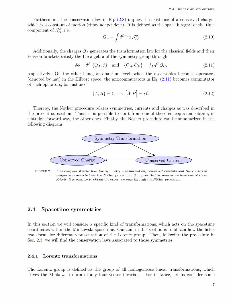
Thereby, the Nother procedure relates symmetries, currents and charges as was described inthe present subsection. Thus, it is possible to start from one of those concepts and obtain, ina straightforward way, the other ones. Finally, the Nother procedure can be summarized in thefollowing diagram
Symmetry Transformation
Conserved CurrentConserved Charge
Figure 2.1: This diagram sketchs how the symmetry transformation, conserved currents and the conservedcharges are connected via the Nother procedure. It implies that as soon as we have one of thoseobjects, it is possible to obtain the other two ones through the Nother procedure.
2.4 Spacetime symmetries
In this section we will consider a specific kind of transformations, which acts on the spacetimecoordinates within the Minkowski spacetime. Our aim in this section is to obtain how the fieldstransform, for different representation of the Lorentz group. Then, following the procedure inSec. 2.3, we will find the conservation laws associated to those symmetries.
2.4.1 Lorentz transformations
The Lorentz group is defined as the group of all homogeneous linear transformations, whichleaves the Minkowski norm of any four vector invariant. For instance, let us consider some
7
2. Global Symmetries
Lorentz transformationx′µ = Λµ
ν xν . (2.13)
Therefore, the Lorentz group is the set of all Λµν matrices satisfying, for an arbitrary vector xµ
xµ ηµν xν = x′µ ηµν x
′ν −→ Λµρ ηµν Λν
σ = ηρσ. (2.14)
Now, in order to define the Lorentz transformation acting on the fields, we need to study howthey transform under such a group. In fact, it is possible to define the transformation law as aninfinitesimal operator by means of the exponential. Let us consider some representation of theLorentz group, φ(x), which transforms according to
φ(x) −→ φ′(x′) = φ′(Λx) ≡ U(Λ)φ(x), (2.15)
where Λx = Λµν x
ν and U(Λ) is the infinitesimal operator we are looking for. Now, the expansion
Λµν = δµν + λµν + . . . , (2.16)
where λµν is an infinitesimal parameter, together with the Eq. (2.14), implies the antisymmetriccondition λµν = −λνµ of such parameter. Thus, using Eq. (2.16) as well as the Taylor expansionof the field φ(x) in Eq. (2.15), we obtain the transformation law under the Lorentz group, interms of the infinitesimal operator
U(Λ) = e−12 λ
µνJµν . (2.17)
Here, Jµν is the generator of the Lorentz transformation in the representation of φ(x), defined ingeneral by means of
Jµν = Lµν1 + Σµν , (2.18)where Lµν = 2x[µ∂ν] and Σµν stand for the orbital and the spin angular momentum generatorsrespectively. Furthermore, in order to obtain an explicit form of the spin generator in someLorentz representation, one need to take the Lorentz transformation of the field,
δφ = −12λ
µνJµνφ, (2.19)
together with its respective action. Then, after an infinitesimal transformation of the fields anddemanding the invariance of its action under such transformation, it is possible to find whichcondition must Σµν satisfy in order to maintain such an invariance. For instance, let Φ be ascalar, V a vector and Ψ a spinor field, then
JµνΦ = LµνΦ,(Jµν)ρ σ V σ =
(Lµνδ
ρσ + 2 δρ[µ ην]σ
)V σ,
JµνΨ =(Lµν1 + 1
2γµν)
Ψ, (2.20)
are found to be the explicit form of the Lorentz generators acting over their different representa-tions. Additionally, the commutators of the Lorentz generators gives
[Jµν , Jρσ] = 4 δ[ρ[µJ
σ]ν]. (2.21)
The conserved current for the Lorentz symmetry can be obtained using the Nother proceduredescribed in the previous section. Thus, using Eq. (2.9) and (2.19) for the Lorentz transformation
8
2.4. Spacetime symmetries
of the representation φ(x), the conserved current for the Lorentz symmetry is
J µ = −12λ
ρσ(2x[ρT
µσ] + σµρσ
)≡ −1
2λρσMµ
ρσ, (2.22)
where we have defined
T µν ≡∂L
∂∂µφ∂νφ− δµνL and σµρσ ≡
∂L
∂∂µφΣρσφ, (2.23)
as the canonical energy-momentum2 and the spin tensor respectively. With these definitions, wecan interpret Mµ
ρσ as the canonical angular momentum tensor, which possess an orbital andspin parts as we can see from Eq. (2.22). Additionally, within the Minkowski spacetime, theconservation law ∂µJ µ = 0 is nothing but the angular momentum conservation which can beread as
∂µMµρσ = 0 or ∂µσ
µρσ = −2T[ρσ], (2.24)
and leads to the Lorentz invariance of the action for the field φ(x).
2.4.2 Poincare transformations
The set of coordinate transformations xµ → x′µ which does not change the form of the metricdefines the isometry group of a given spacetime. The isometry group of the Minkowski spacetimeis the group of global Poincare tranformations and it has the form
xµ −→ x′µ = Λµν x
ν + aµ, (2.25)
where, in addition to the Lorentz transformations, aµ stands for translations. However, it iseasy to implement the translational part of the Poincare group because all the representationstransform in the same way under translations. Let us consider some representation φ(x), whichtransforms under the Poincare group according to
φ(x) −→ φ′(x′) = φ′(Λx+ a) = U(Λ, a)φ(x). (2.26)
Following the same procedure as in the previous section, we obtain
U(Λ, a) = e(aµPµ−12 λ
µνJµν), (2.27)
where Pµ = ∂µ is the generator of translations. Therefore, the infinitesimal Poincare transforma-tion of some representation φ(x) can be written as
δφ =(aµPµ −
12 λ
µν Jµν
)φ, (2.28)
where the Lie algebra of the Poincare group is
[Jµν , Jρσ] = 4 δ[ρ[µJ
σ]ν], (2.29)
[Jµν , Pρ] = 2P[µην]λ, (2.30)[Pµ, Pν ] = 0. (2.31)
2Non-symmetric in general.
9

2. Global Symmetries
Additionally, following the Nother procedure in Sec. 2.3, it is possible to obtain the conservedcurrent for the Poincare symmetry. Thus, using the definitions for the canonical total angularmomentum, Mµ
ρσ, together with the quantities defined in Eq. (2.23), the conserved current forthe Poincare symmetry is
J µ = aνT µν −12λ
ρσMµρσ. (2.32)
Since the infinitesimal parameters aν and λρσ are independent and constant, the conservationlaw of the Poincare current ∂µJ µ = 0, is nothing but the conservation of the energy-momentumand angular-momentum tensor, interpreted as the translational and Lorentz invariance, writtenas
∂µTµν = 0 and ∂µσ
µρσ = −2T[ρσ], (2.33)
respectively.
10
Chapter 3
Differential Geometry
Differential geometry is the natural ground for the generalization of the usual notion of flatEuclidean space. Since the last century, differential geometry has been an important subject ofstudy in mathematics and physics, due to the relation among geometry and gravitation proposedby Einstein. Additionally, the use of differential forms has been widely used along the presentthesis, therefore it is important to give an introduction of such objects and how to deal withthem.
The aim of this chapter is to gather the principal ingredients of differential geometry in orderto build physical theories within the language of differential forms. There exist several excellentbooks which covers these topics in a complete and rigorous way [47–50]. We will follow theapproaches of Refs. [46, 47, 51] and my personal notes on Advanced topics on particle physics II,written throughout the lectures dictated during the fall of 2013 by Dr. Oscar Castillo-Felisola atUTFSM.
3.1 Manifolds
A manifold is a D-dimensional topological space, M, endowed with open sets Ui ⊂ M, calledpatches, which cover M. On each patch, there exist a homeomorphism ϕi which maps thosepatches such that
ϕi : Ui → U ′i ⊂ RD and M =∐i
Ui. (3.1)
Furthermore, the homeomorphism ϕi provides coordinates to each point p ∈M, for instance
ϕi(p) = (x1, . . . , xD) = xµ. (3.2)
In fact, the point p exists on the manifold independently of its coordinates. The pair (Ui, ϕi) iscalled chart while the whole family (Ui, ϕi) is called atlas. In addition, if there exists a secondpatch Uj, such that p ∈ Ui ∩ Uj 6= , then the homeomorphism
ϕj(p) = (x′1, . . . , x′D) = x′µ, (3.3)
provides a second set of coordinates at p. Thus, is required that the map ϕij = ϕiϕ−1j , such that
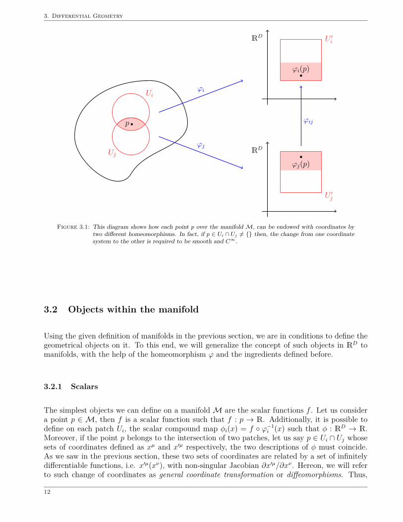
ϕij : RD → RD, is smooth and infinitely differentiable (see figure 3.1). Therefore, a manifold is aD-dimensional topological space which looks locally as RD althought the global structure of suchmanifold (in general) does not.
Cristobal Corral 11
3. Differential Geometry
p
Ui
Uj
ϕi
ϕj
RD
RD
ϕi(p)
U ′i
ϕj(p)
U ′j
ϕij
Figure 3.1: This diagram shows how each point p over the manifold M, can be endowed with coordinates bytwo different homeomorphisms. In fact, if p ∈ Ui ∩ Uj 6= then, the change from one coordinatesystem to the other is required to be smooth and C∞.
3.2 Objects within the manifold
Using the given definition of manifolds in the previous section, we are in conditions to define thegeometrical objects on it. To this end, we will generalize the concept of such objects in RD tomanifolds, with the help of the homeomorphism ϕ and the ingredients defined before.
3.2.1 Scalars
The simplest objects we can define on a manifold M are the scalar functions f . Let us considera point p ∈ M, then f is a scalar function such that f : p → R. Additionally, it is possible todefine on each patch Ui, the scalar compound map φi(x) = f ϕ−1
i (x) such that φ : RD → R.Moreover, if the point p belongs to the intersection of two patches, let us say p ∈ Ui ∩ Uj whosesets of coordinates defined as xµ and x′µ respectively, the two descriptions of φ must coincide.As we saw in the previous section, these two sets of coordinates are related by a set of infinitelydifferentiable functions, i.e. x′µ(xν), with non-singular Jacobian ∂x′µ/∂xν . Hereon, we will referto such change of coordinates as general coordinate transformation or diffeomorphisms. Thus,
12
3.2. Objects within the manifold
the initial scalar field and those with the transformed coordinates must be equivalent such that
φ′(x′) = φ(x). (3.4)
3.2.2 Vectors
In differential geometry, a vector is defined to be a tangent vector to some curve γ : t → M,where t ∈ (a, b), just like a generalization of the velocity vector with respect to some curvec : R → RD. The curve γ lies on the manifold and (a, b) ∈ R. Furthermore, we need a scalarfunction f :M→ R with its domain restricted to the points of γ(t) ∈ M. Then the derivativeof f can be written as
df(γ(t))dt
= ∂f
∂xµ∂xµ
∂t= Xµ
(∂
∂xµ
)f , (3.5)
where xµ stands for the coordinates of the point p ∈ Ui over M, within the domain of γ(t). Wehave used the definition Xµ = ∂xµ
∂tfor the components of the vector field X, while ∂µ = ∂
∂xµ
stands for its basis, i.e. X = Xµ ∂∂xµ
. Notice the definition of the vector field has been doneindependently of the choice of f .
All the equivalent classes of curves at p, thus, all the tangent vectors at p, form a vector spacecalled tangent space of M at p, denoted by TpM. Moreover, if there exist a second patch Uj,such that p ∈ Ui∩Uj and p has coordinates x′ν in such patch, then the components of the secondvector field X ′ = X ′µ ∂
∂x′µare related with the first ones through
X ′µ(x′) = ∂x′µ
∂xνXν(x). (3.6)
From the definition of tangent space, it is clear that the vectors fields lie on it. Nevertheless,we do not expect that the tangent space in some point q 6= p be the same as TpM. Therefore,in order to define vector fields at each point of M we have to consider a new structure calledtangent bundle TM defined as
TM =∐p∈M
TpM. (3.7)
3.2.3 1-forms
In addition to the definition of vector fields which lie on TpM, it is possible to define a linear mapω : TpM → R, as an element of the dual vector space (or cotangent space) denoted by T ∗pM.Such an element is called cotangent vector, or, in the context of differential forms, just 1-form.The simplest case of an 1-form is the differential df , where f stands for a scalar function. If weuse coordinates, the differential can be written as df = ∂f
∂xµdxµ. Therefore, it is rather natural to
identify dxµ as the basis of T ∗pM, thus,
< dxµ, ∂ν >= δµν . (3.8)
Then, defining an arbitrary 1-form as ω = ωµdxµ and regarding the map ω : TpM → R with
V ∈ TpM be an arbitrary vector field, the inner product < •, • > : T ∗pM× TpM→ R of those
13
3. Differential Geometry
objects is defined as< ω, V >= ωµV
µ. (3.9)
Additionally, at each point p ∈ Ui ∩Uj such that xµ = ϕi(p) and x′µ = ϕj(p), the componentsof a 1-form transforms as
ω′µ(x′) = ∂xν
∂x′µων(x). (3.10)
Analogously as in the case of vector fields, the 1-forms live on the cotangent space T ∗pM.However, we do not expect that the cotangent spaces within different points have to be the same.Therefore, we can define a structure where the 1-forms live, called the cotangent bundle T ∗M, as
T ∗M =∐p∈M
T ∗pM. (3.11)
3.2.4 Tensors
Tensors T of type (r, s), are multilinear objects which its basis is constructed using the tensorproduct ⊗ of r tangent space basis times s cotangent space ones. Therefore, it is a map from relements of TpM and s elements of T ∗pM to real numbers and can be written as
T = T µ1...µrν1...νs ∂µ1 ⊗ . . .⊗ ∂µr ⊗ dxν1 ⊗ . . .⊗ dxνs . (3.12)
Following the transformation laws for vectors and 1-forms defined in the previous subsection,it is possible to write the transformation law for tensors under general coordinate transformationsas
T ′µ1...µrν1...νs(x′) = ∂x′µ1
∂xρ1. . .
∂x′µr
∂xρr∂xσ1
∂x′ν1. . .
∂xσs
∂x′νsT ρ1...ρr
σ1...σs(x), (3.13)
while the structure where they live on the manifold is
T rs (M) =(⊗r TpM
)⊗(⊗s T ∗pM
). (3.14)
3.3 Lie derivative
The generalization of the directional derivative of scalar functions on RD, i.e. V ·∇f , where V is avector in RD, to real functions on the manifold is called the Lie derivative. As we will see later, itis possible to generalize this operation to vector and tensor fields. However, in this case it cannotbe interpreted as a directional derivative of neither vector nor tensor fields, since it depends onderivatives of V . Therefore, the interpretation of generalized directional derivative only appliesfor scalar functions on the manifold rather than vector or tensors. In order to transport tensorsalong a curve, we will introduce the covariant derivative in Sec. 3.5.
Let us consider an integral curve γ(t) of X, which means that X is the tangent vector at everypoint of γ(t) ∈ M. Now, at each point q ∈ γ(t) with xµ = ϕ(q), let X be the tangent vector
14
3.4. Differential forms
of γ(t) at q. Then, it is possible to define the Lie derivative LXf(x) of f along X, where f is ascalar function, as
LXf = Xµ∂µf. (3.15)Additionally, it is possible to extend the previous result to vectors V = V µ∂µ and 1-forms (seefor instance [47,49]) as
LXV = (Xµ∂µVν − V µ∂µX
ν) ∂ν , (3.16)LXω = (Xµ∂µων + ωµ∂νX
µ) dxν . (3.17)
Using the previous definitions, the operation of the Lie derivative acting over a (r, s) tensor fieldT is straightforward
LXT =[Xρ∂ρT
µ1...µrν1...νs − T ρµ2...µr
ν1...νs ∂ρXµ1 − . . .− T µ1...µr−1ρ
ν1...νs ∂ρXµr
+ T µ1...µrρν2...νs ∂ν1X
ρ + . . .+ T µ1...µrν1...νs−1ρ ∂νsX
ρ]∂µ1 ⊗ . . .⊗ ∂µr ⊗ dxν1 ⊗ . . .⊗ dxνs .
(3.18)
Moreover, the Lie derivative has the following properties, some of them rather similiar to thoseof the ordinary derivative:
(i) Scalar multiplicationLX(a V ) = aLXV a ∈ R. (3.19)
(ii) Product rule
LX(A⊗B) = (LXA)⊗B + A⊗ (LXB) where A,B ∈ T (M). (3.20)
(iii) Lie bracket of two vector fields X and Y is defined through
LXY = [X, Y ] . (3.21)
Furthermore,[LX ,LY ] = L[X,Y ]. (3.22)
One of the important roles of the Lie derivative is the possibility of writing the infinitesimalcoordinate transformation xµ → x′µ = xµ + ξµ(x) of the fields, in terms of it
δφ(x) = Lξφ(x), (3.23)
where φ stands for scalar, vector, 1-form or tensor field [25,46].
3.4 Differential forms
As we mentioned at the beginning of the present chapter, the language of differential forms hasbeen widely used along this thesis. The advantage of this choice relies on the fact that differentialforms lie on the cotangent bundle and thus, are invariant under the change of coordinates. Forthis reason, the diffeomorphism invariance is guaranteed by means of differential form actionprinciple.
15
3. Differential Geometry
3.4.1 Wedge product
Let us consider some manifoldM, endowed with some tangent TM and cotangent T ∗M bundle.A differential p-form is a completely antisymmetric tensor of type (0, p) which lies on T ∗M andits basis is constructed using the wedge product defined as
dxµ1 ∧ . . . ∧ dxµp =∑σ
(−1)|σ|dxσ(µ1) ⊗ . . .⊗ dxσ(µp), (3.24)
where σ denotes the permutation of the indices. For instance,dxµ ∧ dxν = dxµ ⊗ dxν − dxν ⊗ dxµ,
dxµ ∧ dxν ∧ dxλ = dxµ ⊗ dxν ⊗ dxλ − dxµ ⊗ dxλ ⊗ dxν − dxν ⊗ dxµ ⊗ dxλ
+ dxν ⊗ dxλ ⊗ dxµ + dxλ ⊗ dxµ ⊗ dxν − dxλ ⊗ dxν ⊗ dxµ, (3.25)are the basis of the 2 and 3-form respectively. Additionally, the wedge product defined inEq. (3.24) forms a basis of the vector space of the differential p-forms, denoted by Λp(M).Therefore, an element ω ∈ Λp(M) can be expanded as
ω = 1p!ωµ1...µpdx
µ1 ∧ . . . ∧ dxµp , (3.26)
where hereon bold symbols will denote differential forms.
Let us consider α ∈ Λp(M), β ∈ Λq(M) and γ ∈ Λr(M), then the wedge product ∧ satisfiesthe following properties
dxµ1 ∧ . . . ∧ dxµs = 0 if some index µ is repeated, (3.27)α ∧α = 0 if p is odd, (3.28)α ∧ β = (−1)pq β ∧α, (3.29)
(α ∧ β) ∧ γ = α ∧ (β ∧ γ). (3.30)
3.4.2 Exterior derivative
The exterior derivative d = dxµ ∧ ∂µ, is a map d : Λp(M)→ Λp+1(M) which acts over a p-formω as
dω = 1p! ∂ρωµ1...µp dx
ρ ∧ dxµ1 ∧ . . . ∧ dxµp . (3.31)
For instance, if A = Aµdxµ, then the exterior derivative dA = 1/2 (∂µAν − ∂νAµ)dxµ ∧ dxν .
Additionally, if we consider two differential forms α ∈ Λp(M) and β ∈ Λq(M) the exteriorderivative satisfies the following properties
d(dα) = d2α = 0, (3.32)d(α ∧ β) = (dα) ∧ β + (−1)pα ∧ (dβ). (3.33)
A p-form ω which satisfies dω = 0 is called closed. If ω can be expressed as ω = dχ whereχ ∈ Λp−1(M), then is called exact. In virtue of the nilpotency property defined in Eq. (3.32),any exact form is closed. On the other hand, the Poincare lemma implies that locally any closedform can be expressed as an exact form, but globally it will depend on the topology whether it ispossible or not.
16
3.5. Covariant derivative and connections
3.4.3 Interior product and Lie derivative
The interior product iV is a map iV : Λp(M)→ Λp−1(M) which dependes on the vector field Vand acts over the basis of differential p-form as
iV (dxµ1 ∧ . . . ∧ dxµp) = V µ1dxµ2 ∧ . . . ∧ dxµp − V µ2dxµ1 ∧ dxµ3 ∧ . . . ∧ dxµp+ . . .+ (−1)p V µpdxµ1 ∧ . . . ∧ dxµp−1 . (3.34)
In the same way, can be written acting over a differential p-form ω as
iV ω = 1(p− 1)! V
ρ ωρµ2...µp dxµ2 ∧ . . . ∧ dxµp . (3.35)
The interior product, as well as the exterior derivative, is nilpotent, i.e. iV iV ω = 0. Usingthe definition of the interior product in Eq. (3.35) and the exterior derivative in Eq. (3.31), it ispossible to write the Lie derivative, which is a map LV : Λp(M) → Λp(M), in the language ofdifferential forms as
LV = d iV + iV d. (3.36)For instance, let us calculate the Lie derivative for ω ∈ Λ1(M) using Eq. (3.36), i.e.
LVω = (d iV + iV d)ω = d (V µωµ) + iV12 (∂µων − ∂νωµ) dxµ ∧ dxν ,
= (∂νV µωµ + V µ∂νωµ) dxν + V µ (∂µων − ∂νωµ) dxν ,= (V µ∂µων + ∂νV
µωµ) dxν , (3.37)
which is nothing but the Lie derivative acting on a 1-form, as we defined in Eq. (3.17). Thegeneralization to differential p-forms is straightforward.
3.5 Covariant derivative and connections
As we mention in the Subsec. 3.3, in order to specify how tensor are transported along a curve,we need to define a new operation called covariant derivative, denoted by ∇. In order to achievethis goal, we need to introduce a new structure called connection.
Let us consider a scalar f and three vectors fields X, Y and Z. Then, the covariant derivative∇ satisfies the following conditions
∇X(Y + Z) = ∇X Y +∇X Z , (3.38)∇f(X+Y )Z = f∇X Z + f∇Y Z , (3.39)∇X(fY ) = Xµ (∂µf)Y + f∇X Y. (3.40)
Given a chart (U,ϕ) on a manifoldM, with coordinates xµ = ϕ(p) for each p ∈M, the affineconnection specify how the vector basis change from point to point. As soon as the action of ∇on the vector basis is defined, it is possible to calculate how the ∇ acts on any vector. Let usstart with the definition
∇eµeν ≡ ∇µeν = Γµλν eλ , (3.41)
17
3. Differential Geometry
where eµ = ∂∂xµ
is the basis of TpM. Now, let us consider two vector fields X = Xµ eµ andY = Y ν eν . The covariant derivative of Y along X is defined as
∇X Y = Xµ∇µ (Y ν eν) = Xµ (∂µY ν eν + Y ν∇µeν)= Xµ
(∂µY
λ + ΓµλνY ν)eλ, (3.42)
or written in terms of the λth component of the vector field ∇µY
∇µYλ = ∂µY
λ + Γµλν Y ν . (3.43)
In order to obtain the operation of the covariant derivative acting over 1-forms, we can use thefact that the quantity (V µωµ) transforms as a scalar, therefore ∇µ (V νων) = ∂µ (V νων). Withthis, it is easy to obtain that
∇µων = ∂µων − Γµλν ωλ. (3.44)Following the same argument as before, it is straightforward to obtain the covariant derivativeof a (r, s)-type tensor as
∇µTρ1...ρr
σ1...σs = ∂µTρ1...ρr
σ1...σs + Γµρ1λ T
λρ2...ρrσ1...σs + . . .+ Γµρrλ T ρ1...ρr−1λ
σ1...σs
− Γµλσ1 Tρ1...ρr
λσ2...σs − . . .− Γµλσs T ρ1...ρrσ1...σs−1λ. (3.45)
With this definition, since the covariant derivative does not depends on the derivatives of X,it can be interpreted as the proper generalization of the directional derivative of scalar funtionsto tensor fields.
Additionally, if we introduce a second chart (U ′, ϕ′), such that p ∈ U∩U ′ 6= with coordinatesx′µ = ϕ′(p), then the transformation of the vector basis is e′µ = ∂xν
∂x′µeν . Thus, the new basis
satisfies
Γ′µλν e′λ = ∇e′µe′ν = ∇e′µ
(∂xρ
∂x′νeρ
)= ∂2xρ
∂x′µ∂x′νeρ + ∂xρ
∂x′ν∂xσ
∂x′µΓσαρeα︸ ︷︷ ︸
=∇e′µeρ
,
=(
∂2xρ
∂x′µ∂x′ν∂x′λ
∂xρ+ ∂xβ
∂x′ν∂xσ
∂x′µ∂x′λ
∂xρΓσρβ
)e′λ. (3.46)
Then, comparing both sides of the equation, the transformation for the affine connection Γ underchange of coordinates is
Γ′µλν = ∂xβ
∂x′ν∂xσ
∂x′µ∂x′λ
∂xρΓσρβ + ∂2xρ
∂x′µ∂x′ν∂x′λ
∂xρ. (3.47)
3.5.1 Parallel transport and geodesic
Let us consider some curve γ(t) on a manifold M, such that γ : t → M where t ∈ (a, b). Letus consider, given a chart (U,ϕ), a tanget vector V at every point q ∈ γ(t) with coordinatesxµ = ϕ(q). Then, a vector X is called parallel transported along γ(t) if
∇VX = 0. (3.48)
18
3.6. Riemannian and pseudo-Riemannian manifolds
Additionally, if the tangent vector V is parallel transported along γ(t), let us say
∇V V = 0, (3.49)
the curve γ(t) is called geodesic. In this sense, the geodesic are the straightest possible curves in a(pseudo-)Riemannian manifolds and written in coordinates of γ(t), the equation for the geodesicbecomes
d2xλ
dt2+ Γµλν
dxµ
dt
dxν
dt= 0. (3.50)
3.6 Riemannian and pseudo-Riemannian manifolds
3.6.1 The metric
In this section we will introduce a new structure in order to define the inner product betweenvectors on the manifold M. Such a structure is called metric and we will describe it in thissection. The metric has a rather important role in GR because describes the geometry and thedynamics of the spacetime.
Let M be a differentiable manifold endowed with a chart (U,ϕ). A (pseudo-)Riemannianmetric gµν(p) on M, is a tensor field of type (0, 2) which, at each point p ∈M with coordinatesxµ = ϕi(p), maps g : TpM× TpM→ R and satisfies the following axioms:
(i) Symmetricgµν(p) = gνµ(p). (3.51)
(ii) Positive-definite or non-degenerated
gµν(p)V µV ν ≥ 0, (3.52)
where the equality is satisfied only if V = 0.
(ii’) It is called pseudo-Riemannian if it is symmetric and if
gµν(p)UµV ν = 0 (3.53)
for any U ∈ TpM, then V = 0.
Additionally, since gµν is a map g : TpM× TpM→ R and we have defined the inner productin Subsec. 3.2.3 as a map < •, • > : T ∗pM×TpM→ R, the metric g gives rise to an isomorphismbetween TpM and T ∗pM. Moreover, if we denote the inverse metric as (gµν)−1 = gµν , such thatgµνgνρ = δµρ , we obtain additionally an isomorphism among T ∗pM and TpM due to g−1. Forinstance
gµν Vν = Vµ and gµν ων = ωµ. (3.54)
Using the definition of the metric tensor, we often find in the literature the definition of the lineelement in terms of the metric tensor through
ds2 = gµν dxµdxν . (3.55)
19
3. Differential Geometry
Since the axiom of symmetry is satisfied, the metric tensor possess real eigenvalues. However,if the metric tensor is either Riemannian or pseudo-Riemannian, those eigenvalues are strictlypositive or some of them might be negative, respectively. Moreover, if a differentiable manifoldM is endowed with a metric g, then the pair (M, g) is called Riemannian or pseudo-Riemannianmanifold, depending on which of those metrics is considered.
3.6.2 Metricity condition
In Sec. 3.5 we have not imposed any restriction to the affine connection so far. Since the manifoldswe will consider are endowed with a metric g, we would like to preserve the inner product betweentwo parallel transported vectors along any curve. To achieve this, we need to include a reasonablerestriction to the connection, such as demand that the metric has to be covariantly constant, i.e.
∇µgνλ = 0. (3.56)
This constraint is called the metricity condition. If Eq. (3.56) is satisfied, then the affineconnection Γ is said to be a metric connection. Moreover, cyclic permutations on the in-dices and the splitting of the affine connection into its symmetric and antisymmetric part, i.e.Γµλν = Γ(µ
λν) + Γ[µ
λν] (see Appendix A), allows us to solve an equation for the symmetric part
of the affine connection
Γ(µλν) = 1
2 gλσ(∂µgνσ + ∂νgσµ − ∂σgµν
)+ 1
2(T λµν + T λνµ
). (3.57)
The first parenthesis on the right hand side are the Christoffel symbols while the torsion tensor,i.e. Tµλν = 2Γ[µ
λν], encodes the antisymmetric part of the affine connection. Replacing back the
solution for the symmetric part of the affine connection into its tensor decomposition, we obtain
Γµλν =µλν
+Kµλν , (3.58)
whereµλν
denotes the Christoffel symbols while we have defined the contorsion tensor as
Kµλν = 12(Tµλν + T λµν + T λνµ
). (3.59)
In this sence, the contorsion tensor is said to be the non-Riemannian part of the connection,since it is completely independent of the metric.
3.6.3 The vielbein
The minimal procedure in order to include gravity within theories described by the flat Minkowskispacetime, is first change the Minkowski metric ηµν by the curved one gµν . Further, replace allthe Lorentz tensors by quantities which transforms as a tensor under diffeomorphisms and finallypromote the partial derivative to be a covariant one, as described in Sec. 3.5. Such kind of minimalprocedure works very well for scalars, vectors and tensors because the tensorial representation ofthe GL(D) group, behaves like a tensor under the subgroup of Lorentz transformations. However,this is not the case for the spinorial representation because there is no representation of theGL(D)group which behaves like a spinor under the Lorentz subgroup [52].
20
3.6. Riemannian and pseudo-Riemannian manifolds
In theories of gravity coupled with fermions, it is important the introduction of an additionalobject, called frame field or vielbein,1 which maps the curved space coordinates into tangent spaceones. With such a mapping, it is possible to define spinors as objects lying on the tangent spacewith their proper transformation law under the local Lorentz group.
The equivalence principle allows us to choose a coordinate system which looks locally as aMinkowski space. In other words it is possible to choose a coordinate transformation of a non-inertial observer into an inertial one. This choice can be done by means of the vielbeins eaµ(x),i.e.
gµν(x) = eaµ(x) ηab ebν(x), (3.60)where ηab = diag(−,+, . . . ,+) is the Minkowski metric. Hereon, the latin indices will denoteLorentz (or tangent space) indices while the greek ones stand for diffeomorphism (or generalcoordinates) indices. However, given a metric gµν(x), the choice of the frame field is not unique.All the equivalent choices of the vielbein fields are related by local Lorentz transformations Λa
b(x)as
e′aµ (x) = Λab e
bµ(x). (3.61)
Additionally, Eq. (3.60) requires that the vielbein field transforms as a 1-form under diffeomor-phisms
e′aµ (x′) = ∂xν
∂x′µeaν(x). (3.62)
If the vielbein field is a non-singular matrix, i.e. det eaµ ≡ e =√− det gµν 6= 0, then there exist
an inverse vielbein field Eµa such that Eµ
a ebµ = δab and Eµ
a eaν = δµν . Moreover, the inverse vielbein
field transforms according to
E ′µa (x) = ΛbaE
µb and E ′µa (x′) = ∂x′µ
∂xνEνa (x), (3.63)
under local Lorentz transformations and diffeomorphisms respectively. Moreover, using the in-verse vielbein field, it is possible to rewrite the Eq. (3.60) in terms of
Eµa (x)gµν(x)Eν
b (x) = ηab. (3.64)
Therefore, the inverse vielbein field forms an orthonormal set of vectors on TpM as well as thevielbein fields forms an orthonormal set of 1-forms on T ∗pM. Thus, it is possible to change thecoordinate basis of a (r, s)-diffeomorphism tensor to a Lorentz one, and vice versa, i.e.
T a1...arb1...bs = ea1
ρ1 . . . earρr E
σ1b1 . . . E
σsbsT ρ1...ρr
σ1...σs , (3.65)T ρ1...ρr
σ1...σs = Eρ1a1 . . . E
ρrar e
b1σ1 . . . e
bsσs T
a1...arb1...bs , (3.66)
where latin indices transforms under local Lorentz transformations while the greek ones trans-forms under diffeomorphisms.
Let us consider a manifoldM endowed with a chart (U,ϕ). Taking the components of inversevielbein field at some point p ∈ M, with coordinates xµ = ϕ(p), it is possible to construct thevector basis on the tangent space as
Ea = Eµa
∂
∂xµ. (3.67)
1Vielbein means “many legs” in german and we will use it for D-dimensional spacetimes. However, we often find in the literaturenames like dreibein, vierbein and so on, in 3 and 4-dimensional spacetimes respectively.
21
3. Differential Geometry
In general, the commutator of two vector basis defined in this form, can be written as2
[Ea, Eb] = −Eµa E
νb
(∂µe
cν − ∂νecµ
)Ec ≡ Ωab
cEc, (3.68)
where Ωabc = ecµLEaEµ
b are the frame components of the Lie bracket, which does not vanishes ingeneral and are called anholonomy coefficients [46].
Analogously, we can also use the vielbein field to construct a new basis for the vector spaceΛp(M) of differential forms. This means that the vielbein 1-form,
ea = eaµ dxµ, (3.69)
can be used as a basis of differential forms, as well as dxµ. For instance, it is possible to define adifferential p-form using
ω = 1p!ωµ1...µp dx
µ1 ∧ . . . ∧ dxµp = 1p! ωa1...ap ea1 ∧ . . . ∧ eap . (3.70)
3.6.4 Integration of differential forms
As it is well known, the equations of motion of some physical system can be derived from anaction principle. In order to build such an action within the language of differential forms, weneed to define how to perform the integration of p-forms. In a D-dimensional manifold M,endowed with a chart (U,ϕ) with local coordinates xµ = ϕ(p), where p ∈ M, it is only possibleto integrate D-forms
I =∫Mω = 1
D!
∫Mωµ1...µD dx
µ1 ∧ . . . ∧ dxµD =∫Mω01...D−1 dx
0dx1 . . . dxD−1, (3.71)
where in the last equality we have used the fact that ωµ1...µD(x) possess in fact, only one inde-pendent component. Hereon, it is possible to perform the usual integration using multi-variablecalculus.
Additionally, if we consider a second chart (U ′, ϕ′) such that U ∩ U ′ 6= and with localcoordinates x′µ = ϕ′(p), then the integral I in Eq. (3.71) transforms as
I → I ′ = 1D!
∫M′
ω′µ1...µD(x′) dx′µ1 ∧ . . . ∧ dx′µD = I (3.72)
under coordinate transformation and therefore it is invariant under diffeomorphisms.
In order to define the canonical volume form, we need to define the Levi-Civita alternatingsymbol in local coordinates as
εa1...aD =
+ 1, for even permutation of a1 . . . aD,
− 1, for odd permutation of a1 . . . aD,
0, if any of the indices apperars repeated at least once.(3.73)
In fact, the Levi-Civita symbol, written in local coordinates, transforms as a tensor under properLorentz transformation, i.e. det Λa
b = 1 and their indices can be raised using the inverse of the2Here we have used the identity ∂µ
(Eνb e
bλ
)= 0 = ∂µEνb e
bλ + Eνb ∂µe
bλ.
22
3.6. Riemannian and pseudo-Riemannian manifolds
Minkowski metric ηab. Henceforth, we will use the normalization ε01...D−1 = 1 = − ε01...D−1 alongthis thesis.
The Levi-Civita alternating symbol can be used to define the determinant of any D×D matrixMa
b asdetM εa1...aD = εm1...mD M
m1a1 . . .M
mDaD . (3.74)
Further, it is possible to define the Levi-Civita tensor density by means of the vielbein field andits determinant det eaµ ≡ e = √−g where g = det gµν , as
εµ1...µD = e−1 ea1µ1 . . . e
aDµDεa1...aD , (3.75)
εµ1...µD = eEµ1a1 . . . E
µDaDεa1...aD . (3.76)
Thus, using the definitions given in this section, it is possible to write the so-called canonicalvolume D-form defined as
dV = dDx√−g = dDx e = 1
D! εa1...aD ea1 ∧ . . . ∧ eaD = 1D! e εµ1...µD dx
µ1 ∧ . . . ∧ dxµD . (3.77)
On the other hand, if we consider the useful identity for the contraction of the Levi-Civita tensor
εa1...apc1...cq εb1...bpc1...cq = − p! q! δa1[b1. . . δ
apbp], (3.78)
together with the definition of the canonical volume form on a D-dimensional manifold M, wearrive to the identity
ea1 ∧ . . . ∧ eaD = −εa1...aD e dDx. (3.79)
3.6.5 Hodge duality and inner product between forms
Another useful operation between forms is the Hodge duality ? which acts on the basis of differ-ential forms ω ∈ Λp(M). If the manifold M is endowed with a metric gµν , the Hodge dual is amap ? : Λp
M −→ ΛD−pM from p to (D − p)-forms. Then, the Hodge dual acting over differential
form basis is defined as
? (dxµ1 ∧ . . . ∧ dxµp) =√−g
(D − p)! εµ1...µp
νp+1...νD dxνp+1 ∧ . . . ∧ dxνD
or ? (ea1 ∧ . . . ∧ eap) = 1(D − p)! ε
a1...apap+1...aD eap+1 ∧ . . . ∧ eaD . (3.80)
Since the Hodge duality is a map from p to (D−p)-forms, is useful to write the inner productsbetween p-forms because, it is only possible to integrate D-forms in a D-dimensional manifoldM. Suppose a simple example, let A and B be both 1-forms, then∫
A ∧ ?B =∫
(Aa1ea1) ∧Bb1
εb1c2...cD
(D − 1)!ec2 ∧ . . . ∧ ecD =
∫Aa1B
b1εb1c2...cD
(D − 1)!ea1 ∧ ec2 ∧ . . . ∧ ecd ,
=∫dDx√−g AµBµ =
∫dDx eAaB
a,
where in the last line we have used the Eq. (3.79) and Eq. (3.78). Therefore, given a manifoldM endowed with a metric g, it is possible to write the scalar product between p-forms, by means
23
3. Differential Geometry
of the Hodge dual. Additionally, in the same spirit of the conventional inner product betweenvectors, the inner product between forms is symmetric, i.e.∫
A ∧ ?B =∫B ∧ ?A. (3.81)
3.7 Cartan’s structure equations
In this section, the review of the Cartan’s structure equations will be done as well as the introduc-tion of new objects, such as the Lorentz connection. The structure equations relates the vielbeinsand the Lorentz connection with the torsion and the Lorentz curvature 2-forms, respectively, aswe will see throughout this section.
3.7.1 The first structure equation
In order to start with, let us examine the exterior derivative of the vielbein 1-form under localLorentz transformations as
de′a = d(Λa
b eb)
= dΛab ∧ eb + Λa
b deb. (3.82)
The first term on the right-hand-side of the Eq. (3.82), spoils the vector transformation of thevielbein’s derivative. Then, following the procedure of Sec. 3.5 or analogously as we will seein the Chap. 4, we need to include a connection in order to compensate the extra contributioncoming from the derivative of the local transformation. Since the transformation belongs to thelocal Lorentz group, we will call this structure the Lorentz connection 1-form, denoted by ωab =ωµ
ab dxµ. So, let us consider the covariant derivative, with respect to the Lorentz connection, ofthe vielbein field as
Dea = dea + ωab ∧ eb = T a = 12Tµ
aν dx
µ ∧ dxν , (3.83)
where T a is the torsion 2-form and it does not vanishes in general as we saw in the Subsec. 3.6.2.Additionally, the Eq. (3.83) is called the first Cartan’s structure equation. Thus, if ωab transformsunder local Lorentz transformations as
ωab −→ ω′ab = Λac dΛc
b + Λacω
cd Λd
b, (3.84)
then the Lorentz covariant derivative of the vielbein field and, therefore, the torsion 2-form,transforms as a vector under local Lorentz transformations, i.e. (Dea)′ = Λa
b (Dea) and T ′a =Λa
bT b.
On the other hand, if we restrict ourself to the proper Lorentz group, i.e. det Λab = 1, the
transformation law for the Lorentz connection on Eq. (3.84), follows the same properties as theYang-Mills gauge potential for the group SO(1, D − 1). Therefore, the invariance under localLorentz transformation is implemented through the Lorentz connection ωab. For instance, let usconsider some p-form Lorentz valued (r, s)-tensor T a1...ar
b1...bs(x), i.e.
T ′a1...arb1...bs(x) = Λa1
m1 . . .Λarmr Λn1
b1 . . .Λnsbs T
m1...mrn1...ns(x), (3.85)
24
3.7. Cartan’s structure equations
then the covariant derivative of such a tensor is
DT a1...arb1...bs = dT a1...ar
b1...bs + ωa1cT
ca2...arb1...bs + . . .+ ωar cT a1...ar−1c
b1...bs
− ωcb1Ta1...ar
cb2...bs − . . .− ωcbsT a1...arb1...bs−1c. (3.86)
On the other hand, spinors plays a rather important role in physical theories. As we have seenin Chap. 2, they transform non-trivially under global Lorentz transformations. Moreover, as wasargued at the beginning of the Subsec. 3.6.3, spinors are objects which lie on the tangent space.Then, if we consider local Lorentz transformation of spinors fields, their transformation law is
Ψ′(x) = e−14λabγab Ψ(x). (3.87)
Thereby, their Lorentz covariant derivative is
DΨ = dΨ + 14ω
abγabΨ, (3.88)
where ωab follows the transformation law in Eq. (3.84). With such a covariant derivative, it is pos-sible to construct a Dirac action which is invariant under local SO(1, D − 1) group. Furthermore,let us consider the covariant derivative of the Minkowski metric, then
Dηab = dηab − ωcaηcb − ωcbηac = −ωba − ωab = 0. (3.89)
This means that the Minkowski metric is an invariant tensor of the Lorentz group. Therefore,the scalar products V aωa, are preserved under parallel transport with respect to the Lorentzconnection.
3.7.2 Lorentz connection decomposition
It is quite often to find in the literature theories of gravity which deal with torsion-free metricconnections. Such an object is called the Levi-Civita connection and satisfy the condition
dea + ωab ∧ eb = 0, (3.90)
where hereon ringed quantities will denote torsion-free ones. However, there exist theories ofgravity where the torsion tensor appears as a nonvanishing quantity. For such cases, it is im-portant to decompose the Lorentz connection into its torsion-free and torsionful components,i.e. ωab = ωab +Cab. In order to find the explicit form of Cab, we can rewrite the Eq. (3.83) incoordinates, by means of the vielbein fields as
Tµλν = Ωλ
[µν] + (ωµ)λ ν − (ων)λ µ, (3.91)
where we have used the definitions
Ωλ[µν] = 2Eλ
a ∂[µeaν] and (ωµ)λ ν = (ωµ)a b ebν Eλ
a . (3.92)
Note that (ωµ)λ ν is antisymmetric in the last two indices. Additionally, the torsion-free conditionin Eq. (3.90) written in coordinates reads
Ωλ[µν] + (ωµ)λ ν − (ων)λ µ = 0, (3.93)
25
3. Differential Geometry
which gives an extra constraint. Then, after performing 2 cyclic permutation on the indices inEq. (3.91), we obtain 2 extra equations. Adding them, we get
Tµλν − Tνµλ + T λνµ = Ωλ[µν] +
(ωµ)λ
ν −(ων)λ
µ − Ωµ[νλ] −
(ων)µ
λ +(ωλ)µν
+ Ων[λµ] +
(ωλ)νµ−(ωµ)ν
λ. (3.94)
Now, by means of the decomposition ωµab = ωµab +Cµ
ab, the torsion-free condition in Eq. (3.90)
and the fact that Cµab is antisymmetric in its last two indices, it is possible to find a uniquesolution of the Eq. (3.94) and it is
Cµλν = 1
2(Tµλν + T λµν + T λνµ
). (3.95)
Comparing with Eq. (3.59), we conclude that Cµλν is nothing but the contorsion tensor studied inthe Subsec. 3.6.2 and hereon we will denote it as K instead of C. Additionally, the decompositionof the Lorentz connection 1-form into their torsion-free part plus the contorsion tensor, i.e.
ωab = ωab + Kab, (3.96)
together with the Eq. (3.90), leads to the following relation among the torsion 2-form and thecontorsion 1-form
T a = Kab ∧ eb. (3.97)
Additionally, in the 4-dimensional case, it is useful to split the torsion tensor into its irreduciblecomponents3 as
Tabc = 23T[aηc]b −
13!εabcdS
d + qabc, (3.98)
where Ta ≡ Tamm and Sd ≡ εlmndTlmn denotes the vector and axial component of the torsion tensorrespectively. The last term qabc is a mixed tensor which satisfies the relations qamm = 0 = εlabcqabc.
3.7.3 The second structure equation
As we identify previously, the Lorentz connection possess the same transformation property asthe SO(1, D − 1) Yang-Mills gauge potential. Therefore, it is possible to define the Lorentzfield strength associated to such connection, by acting the covariant derivative twice on a p-formLorentz-valued vector field4 V a
DDV a = RabV
b, (3.99)where we have defined
dωab + ωac ∧ ωcb = Rab = 1
2 Rab µν dx
µ ∧ dxν , (3.100)
as the Lorentz curvature 2-form, which is a Lorentz-valued (1, 1)-tensor while Eq. (3.100) is calledthe second Cartan’s structure equation.
3Such a decomposition is quite useful because the irreducible components does not mix each other.4Since we are working with the antisymmetric basis of differential forms, the Lorentz covariant derivative acting twice over a p-form
Lorentz-valued vector field, is analogous to demand [Dµ, Dν ]V a = Rab µν V b, where Rab µν = 2∂[µων]ab + 2ω[µ|
ac ωc|ν]b.
26
3.7. Cartan’s structure equations
As was pointed out by Cartan in Refs. [21–23], the local properties of a manifold M iscompletely determined by their Lorentz curvature and torsion. Moreover, both objects are inde-pendent geometrical quantities.
If we use the Lorentz connection decomposition in Eq. (3.96) and the Eq. (3.100), we obtainthe following identity for the Lorentz curvature
Rab = Rab + DKab + Ka
c ∧Kcb, (3.101)
whereR
ab = dωab + ωac ∧ ωcb = 12Rab
µν dxµ ∧ dxν (3.102)
is the Riemannian curvature 2-form and it is related with the Riemann curvature tensor viaRρσ
µν = Rabµν E
ρa E
σb while D denotes the torsion-free covariant derivative, i.e. Dea = 0.
3.7.4 Bianchi identities
Within the language of differential forms, it is straightforward to obtain the Bianchi identities forthe torsion and the Lorentz curvature 2-forms. To achieve this goal, we need to take the Lorentzcovariant derivative on both sides of Eqs. (3.83) and (3.100), which gives us
DT a = Rab ∧ eb and DRab = 0, (3.103)
respectively.
3.7.5 Relations between formalisms
As we have seen, the affine connection is needed to construct the covariant derivative of tensorswith respect to the group of diffeomorphisms, while the Lorentz connection is needed to achievethe same goal but for local Lorentz tensors. However, both connections are related. To see this,let us start with the vielbein postulate
∂µeaν − Γµλνeaλ + ωµ
abebν = 0, (3.104)
which is nothing but the vanishing covariant derivative of the vielbein field, with respect to itstwo indices. This equation has as a solution for either the affine or for the Lorentz connection as
Γµλν = Eλa
(∂µe
aν + ωµ
ab e
bν
)or ωµ
ab = eaλ
(∂µE
λb + Γµλν Eν
b
), (3.105)
respectively. In fact, using such solutions and the vielbein postulate, one obtains the metricitycondition in Eq. (3.56). Additionally, if we consider ∇µ and Dµ as the covariant derivatives withrespect to the affine and Lorentz connection respectively, we can find a relation between themusing the Eq. (3.105) and
∇µVν = ∂µV
ν + Γµνλ V λ = ∂µVν + Eν
a
(∂µe
bλ + ωµ
ab e
bλ
)V λ,
= Eνa Dµ
(eaρ V
ρ)
= Eνa DµV
a. (3.106)
Such a property can be generalized to (r, s)-tensors in a straightforward way
∇µTρ1...ρr
σ1...σs = eρ1a1 . . . e
ρrar E
b1σ1 . . . E
bsσs Dµ T
a1...arb1...bs . (3.107)
27
3. Differential Geometry
3.8 Actions in physics
The aim of this section is to write, using the language of differential forms, the different physicalactions we will find throughout this thesis. In order to achieve this, we will use the relations andidentities studied in the present Chapter. As we defined before, bold symbols denotes differentialforms and, hereon, the wedge product between forms will be implicit.
3.8.1 The scalar field’s action
The simplest action we often find in the literature is the action for the scalar field. Let us startwith the following action written in differential forms and we will show that it is equivalent totheir well known coordinate counterpart.
Proposition 1.
SΦ = −12
∫dΦ ? dΦ = −1
2
∫dDx√−g ∂µΦ ∂µΦ. (3.108)
Proof 1. We will start from the first equality and show that it is equal to the second one,
−12
∫dΦ ? dΦ = −1
2
∫(∂mΦ em) ? (∂a1Φ ea1) ,
= −12
∫(∂mΦ em) ∂a1Φ εa1
a2...aD
(D − 1)! ea2 . . . eaD ,
= −12
∫(∂mΦ) ∂a1Φ εa1a2...aD
(D − 1)!(−εma2...aD e dDx
),
= −12
∫dDx√−g ∂µΦ ∂µΦ,
where in the last line we have used the identity for the contraction of the antisymmetric symbolsin Eq. (3.78), e = √−g and the fact that V aVa = V µVµ. Thus, both actions are equivalent.
3.8.2 Abelian gauge field’s action
The Maxwell’s theory of electrodynamics, is successfully described by the U(1) gauge theory. Letus find an action, written in differential forms, for the kinetic term of the Abelian gauge fields.
Proposition 2. Let us consider the U(1) gauge field 1-form A = Aa ea = Aµ dxµ. Then, using
differential forms, it is possible to define the field strength associated to such a gauge field, in acompact way as F = dA, where in coordinates is nothing but the usual Fµν = 2 ∂[µAν]. Let usstate the following proposition
SEM = −12
∫F ? F = −1
4
∫dDx√−g FµνF µν . (3.109)
28
3.8. Actions in physics
Proof 2. Starting with the first equality
−12
∫F ? F = −1
2
∫ (12 Flm el em
)?(1
2 Fn1n2 en1 en2
),
= −18
∫ (Flm el em
)Fn1n2
εn1n2n3...nD
(D − 2)! en3 . . . enD ,
= −18
∫Flm F
n1n2εn1...nD
(D − 2)!(−εlmn3...nD e dDx
),
= −14
∫dDx√−g FµνF µν ,
where in the last line, we have used the same identities as in the Proof 1. Therefore, we find thatthis two descriptions are equivalent.
3.8.3 Non-Abelian gauge field’s action
The SM of particle physics, is described by the gauge group SU(3)C × SU(2)L × U(1)Y , whereSU(3) and SU(2) are non-Abelian gauge groups. The first authors who worked on the SU(2)group of isospin were Yang and Mills [9], therefore we will call to this gauge theory Yang-Millstheory.Proposition 3. Let us consider the SU(N) gauge field 1-form A = TAAAa ea = TAAAµ dxµ,where TA are the generators of the Lie algebra associated to the SU(N) gauge group. Thosegenerators satisfies [TA, TB] = ı fAB
C TC and Tr [TA TB] = 1/2 δAB (see Appendix B), where fABCare the real structure constant of the group while the capital latin indices A,B,C stands for theSU(N) indices. Analogously to the Abelian case, it is possible to write the non-Abelian gaugefield strength F = dA + A ∧A, then
SYM = −∫
Tr [F ?F ] = −14
∫dDx√−gFAµν FµνA . (3.110)
Proof 3. Starting with the first equality
−∫
Tr [F ?F ] = −∫
Tr [TA TB] FA ?FB,
= −∫ 1
2δAB(1
2 FAlm el em
)?(1
2FBn1n2 en1 en2
),
= −18
∫ (FAlmFAn1n2
)el em
εn1n2n3...nD
(D − 2)! en3 . . . enD ,
= −18
∫ (FAlmFn1n2
A
) εn1...nD
(D − 2)!(−εlmn3...nD e dDx
),
= −14
∫dDx√−gFAµν FµνA ,
we find that both actions are equivalent.
3.8.4 Dirac field’s action
As we said in Subsec. 3.6.3, the natural ground in order to couple spinors to gravity is the vielbeinformalism. The Dirac fields represent fermions in the SM, then it is important to write its action
29
3. Differential Geometry
using differential forms.
It is worth to note that in the torsion-free description of gravity, the usual Dirac action or theHermitian one are equivalent, since the addition of the Hermitian conjugate in the kinetic termof the Dirac action, is just a boundary term plus the usual one which appears in the QFT books.Thus, there is no difference between the election of those two actions. However, this is not thecase in torsionful gravity, because there exist a contribution in Hermitian Dirac action comingfrom the interaction of torsion trace with the fermionic vector current (see Appendix C). In sucha case, both actions differ from each other when the integration by parts is performed. For thisreason, we will use the Hermitian Dirac action in gravity with torsion, in order to maintain theunitarity of the theory, even if on-shell the torsion trace vanishes.
Proposition 4. Let us consider a spinor field Ψ and a set of gamma matrices satisfying theClifford algebra γµ, γν = 2 gµν. Then the Dirac action can be written as
SΨ = −12
∫ (Ψγ ?DΨ−DΨ ? γΨ
)= −1
2
∫dDx√−g Eµ
a
(ΨγaDµΨ−DµΨγaΨ
), (3.111)
where γ = γaea is the gamma matrix 1-form.
Proof 4. Starting from the first equality
−12
∫ (Ψγ ?DΨ−DΨ ? γΨ
)= −1
2
∫ (Ψ (γaea) ?
(Db1Ψeb1
)−(DaΨea
)?(γb1eb1
)Ψ),
= −12
∫ (ΨγaDb1Ψ−DaΨγb1Ψ
)ea
εb1b2...bD
(D − 1)! eb2 . . . ebD ,
= −12
∫ (ΨγaDb1Ψ−DaΨγb1Ψ
)εb1...bD
(D − 1)!(−εab2...bD e dDx
),
= −12
∫dDx√−g Eµ
a
(ΨγaDµΨ−DµΨγaΨ
),
where, in the last line, we have used the same identities as in the Proof 1, together with γa = Eaµγ
µ.Thereby, both descriptions of the Dirac action are equivalent.
3.8.5 Einstein-Cartan’s action
The minimal extension of GR towards a theory which includes torsion, is the Einstein-Cartantheory. The action which describes such a theory, is nothing but the Einstein-Hilbert one althoughconstructed using an affine connection which possess an antisymmetric non-Riemannian part, aswe saw in Sec. 3.5. In this Subsection, we will write it using differential forms.
Proposition 5. Let us consider the Lorentz curvature described in Eq. (3.100). Then, theEinstein-Cartan action can be written as
SEC = 12κ2
∫ εa1...aD
(D − 2)! Ra1a2 ea3 . . . eaD = 12κ2
∫dDx√−gR , (3.112)
where κ is related with the fundamental Planck scale M∗, in D = 4 + m dimensions, throughκ2 = M
−(2+m)∗ and R = gµνRµν where Rµν = Rµ
λνλ.
30
3.8. Actions in physics
Proof 5. Starting with the action written in differential forms1
2κ2
∫ εa1...aD
(D − 2)! Ra1a2 ea3 . . . eaD = 12κ2
∫ εa1...aD
(D − 2)!12 R
a1a2lm el em ea3 . . . eaD ,
= 12κ2
∫ εa1...aD
(D − 2)!12 R
a1a2lm
(−εlma3...aD e dDx
),
= 12κ2
∫dDx√−gR ,
where R = Rablmδ
laδmb is constructed using a connection which possess torsion. Therefore, we
find the Einstein-Cartan action written in differential forms.
31

3. Differential Geometry
32
Chapter 4
Gauge Symmetries
As we studied in the Chap. 2, the concept of global symmetries has been a rather useful toolto obtain the conserved quantities of the physical systems. However, since 1929, the idea ofdescribing the interactions with either Abelian (Fock [5], London [6], Weyl [7] and Pauli [8]) ornon-Abelian (Yang and Mills [9]) gauge symmetries, it has become a widely studied topic amongphysicists.
The proposal is basically localize the parameter of the global symmetry, i.e. the parameterof such a symmetry is promoted to depend on their coordinates, for instance θA → θA(x).Nevertheless, this procedure spoils the covariant transformation of the derivative of some group’srepresentation, because there appears an extra term coming from the local parameter’s derivative.Therefore, in order to eliminate such an extra contribution and obtain a theory which is invariantunder local transformations, we need to include a compensating field in the derivative, calledgauge connection. If the connection transforms in a particular way, it will eliminate the extracontribution and, therefore, the theory will be invariant under such a local transformation group.As we will see, the transformation law of the gauge connection is rather similar to that we havestudied in Sec. 3.5, although for a different local group. In this sense, this new derivative of somegroup’s representation, transforms covariantly under the gauge group. Then, in the same spiritof Sec. 3.5, we will call to this object the gauge covariant derivate.
Throughout this chapter we will follow the approches of Refs. [53], even though we will widelyuse differential forms. Moreover, for the Poincare Gauge Theory (PGT) we will follow, addition-ally, the approach of Refs. [25,46].
4.1 Abelian gauge theory
As it is known from Ref. [7], Quantum Electrodynamics (QED) can be formulated as an U(1)Abelian gauge theory. In order to achieve this, one starts from an action principle and demandsthe invariance of such theory under a gauge transformation. Let us consider a U(1) gauge trans-formation of some representation φ(x), which is nothing but the change under an infinitesimallocal phase as
φ(x) −→ φ′(x) = eı θ(x) φ(x). (4.1)
The kinetic term of the representation φ(x), is constructed by means of its derivatives. For
Cristobal Corral 33
4. Gauge Symmetries
instance, let us consider the exterior derivative acting over a transformed field
dφ(x) −→ dφ′(x) = d(eı θ(x) φ(x)
)= eı θ(x)
(ıdθ(x)φ(x) + dφ(x)
). (4.2)
Note that the first term on the last equality spoils the covariant transformation of the field’sderivative under the U(1) gauge symmetry. Therefore, in order to obtain a derivative whichtransform covariantly under U(1) gauge symmetry, we need to endow such a derivative with agauge connection. Then, if the connection transforms properly under the gauge group, it willeliminate the extra contribution coming from the parameter’s derivative. Such an object is calledgauge covariant derivate D and it is defined as
Dφ(x) =(d + ı qA
)φ(x). (4.3)
Here we have definedA = Aµdxµ as the 1-form U(1) gauge connection, while q is a free parameter
which will be identified with the electromagnetic charge. Now, in order to obtain an invariantaction, we demand that the gauge covariant derivative transforms in the following way
Dφ(x) −→(Dφ(x)
)′= eı θ(x)Dφ(x). (4.4)
Hence, using the Eq. (4.3) and Eq. (4.4), is easy to obtain the transformation of the gauge fieldunder U(1) gauge transformations
A(x) −→ A′(x) = A(x)− 1q
dθ(x). (4.5)
Therefore, if we consider the gauge transformation law in Eq. (4.1) and Eq. (4.5), together withthe covariant derivative defined in Eq. (4.3), it is possible to obtain an invariant theory underU(1) gauge transformations.
For instance, let us consider the fermionic action in absence of gravity1
SΨ = −12
∫ (Ψγ ?DΨ−DΨ ? γΨ
)= −1
2
∫ (Ψγ ? dΨ− dΨ ? γΨ
)− ı q
∫ΨγΨ ?A. (4.6)
After its suitable quantization, this action describes Quantum Electrodynamics (QED), writtenwithin the language of differential forms. Therefore, by construction, the action SΨ is invariantunder the gauge transformations.
As usual, the gauge field strength associated to the U(1) connection, can be obtained by meansof the gauge covariant derivatives, acting twice on some representation φ(x) as2
DDφ(x) = ı qFφ(x), (4.7)where F = dA. Additionally, considering the transformation law for the gauge fields in Eq. (4.5),is easy to check that the field strength F is invariant under gauge transformations, i.e
F −→ F ′ = F . (4.8)Then, considering the ingredients throughout this Section and the definition of the Abelian gaugeaction in Subsec. 3.8.2, it is possible to write, the renormalizable gauge invariant action for QED(in absence of gravity) as
SQED = −12
∫ (Ψγ ? dΨ− dΨ ? γΨ
)− ı q
∫ΨγΨ ?A− 1
2
∫F ? F . (4.9)
1We have neglected gravity in this Section for sake of simplicity. However, we will include it later.2As we saw in the Subsec. 3.7.3, this is analogous to demand the commutator of two gauge covariant derivatives acting on some
representation φ(x), i.e. [Dµ,Dν ]φ = ı q Fµνφ, where Fµν = 2∂[µAν].
34
4.2. Non-Abelian gauge symmetry: Yang-Mills theory
4.2 Non-Abelian gauge symmetry: Yang-Mills theory
As was pointed out before, Yang and Mills [9] extended the idea of gauge symmetries to non-Abelian groups. In particular, they studied the case of the SU(2) gauge group of isospin. Thiswas a rather important achievement for the nowadays physics, since the color and electroweaksectors of the Standard model are described by non-Abelian gauge groups.
Let us consider some representation φ(x) of the SU(N) gauge group which transforms as
φ(x) −→ φ′(x) = eı θA(x)TAφ(x), (4.10)
under gauge transformations, where θA(x) are real infinitesimal local functions of the spacetimecoordinates, while TA are the generators of the Lie algebra associated with the SU(N) group.The capital Latin indices, A = 1, . . . , (N2−1), stands for the SU(N) indices while the generatorssatisfies the Lie algebra
[TA, TB] = ı fABC TC , (4.11)
where fABC ∈ R are the structure constants of the Lie algebra. In order to relax the notation,the matrix indices has been omitted, keeping in mind that TA are N × N matrices while therepresentation φ(x) is a column vector with N components.
As was argued for Abelian gauge theories, in order to include the dynamical content of thefields, we need to promote a derivative which transforms covariantly under gauge transformations.Following the similar procedure as in the Abelian case, the SU(N) gauge covariant derivativecan be defined as
Dφ(x) =(d + ı g TA AA(x)
)φ(x), (4.12)
where AA(x) = AAµdxµ is the SU(N) gauge connection while g is a real parameter. The covariantderivative D transforms properly under the gauge transformations if satisfies the condition
Dφ(x) −→(Dφ(x)
)′= eı θ
A(x)TA(Dφ(x)
). (4.13)
Now, using the expansion eı θA(x)TA = 1+ ı θA(x)TA for θA(x) 1 and the commutation relationin Eq. (4.11), it is possible to obtain the transformation law for the gauge the connection AA
under gauge transformations, from Eq. (4.13) as
TA AA −→(TA AA
)′= TA AA − fABC θA AB TC −
1gTA dθA. (4.14)
The gauge field strength can be obtained, as usual, acting the gauge covariant derivative twiceon a representation φ(x) of the SU(N) group3
DDφ(x) = ı gF φ(x) (4.15)
where we have defined F = dA + ı gA ∧A, with A = TAAAµ dxµ, as the non-Abelian gaugefield strength. Similiar to the Abelian case, the field strength F is invariant under the gaugetransformation (4.14), i.e. F → F ′ = F .
3Or analogously using coordinates, it reads [Dµ,Dν ]φ = ı g TA FAµν , where FAµν = 2∂[µAAν] − g fBCAABµ ACν .
35
4. Gauge Symmetries
For instance, let us consider the case of fermions minimally coupled to the non-Abelian gaugefields in absence of gravity. Additionally, we can include the kinetic term for the non-Abeliangauge fields, described in Subsec. 3.8.3. Thus, the action for the Yang-Mills theory, written indifferential forms, is
SYM = −12
∫ (Ψγ ? dΨ− dΨ ? γΨ
)− ı g
∫ΨTAγΨ ?AA −
∫Tr [F ?F ] , (4.16)
and, as was showed by ’t Hooft and Veltman in Refs. [10–12], it is a renormalizable theory, evenin the broken phase when the gauge bosons get massive.
4.3 Local spacetime symmetries: Poincare Gauge Theory
As it was showed in Subsec. 2.4.2, the transformation law of a representation φ(x), under theglobal Poincare group is
δφ =(aµPµ −
12λ
µνJµν
)φ =
(aµ + λµνxν
)∂µφ−
12λ
abΣabφ , (4.17)
where λab = eaµ ebν λ
µν . Let us consider ξµ = aµ + λµνxν and λab as a basis of independenttransformations. The localization of the Poincare group can be addressed promoting their 10independent parameters to be functions of the spacetime, i.e. ξµ → ξµ(x) and λab → λab(x).Here, the orbital part of the Lorentz transformation, i.e. Lµν , has been included in the definitionof ξµ(x) while the spin part, Σab, has been written using local coordinates in order to identifythe function λab(x) as the local Lorentz transformations. Thus, the transformation of somerepresentation φ(x) under the local Poincare group can be written as
δφ = ξµ(x)∂µφ−12λ
ab(x)Σabφ. (4.18)
The key point of local Poincare transformations is to identify the general coordinate trans-formations with local translations and, additionally, only the fields which possess local Lorentzindices, transforms under local Lorentz transformations. For instance, let us consider a scalarΦ(x), vector Vµ(x) and spinor field Ψ(x). In order to obtain their transformation laws under thelocal Poincare group, we will use the explicit form of the spin generator Σab for each representa-tion, as was obtained in Subsec. 2.4.1. Thus, the transformations under the local Poincare groupreads
δΦ =(aµ∂µ −
12λ
µνJµν
)Φ = ξµ(x)∂µΦ,
δVµ =(δνµ a
ρ∂ρ −12λ
ρσ (Jρσ)µν)Vν = ξρ(x)∂ρVµ − λµνVν ,
δΨ =(aµ∂µ −
12λ
µνJµν
)Ψ = ξµ(x)∂µΨ− 1
4λab(x)γabΨ, (4.19)
for the scalar, vector and spinor field respectively. However, using the identity ∂µξν(x) = −λµν ,it is possible to express the transformation law for the scalar and vector field by means of theLie derivative with respect to the vector field ξµ(x), i.e.
δΦ = ξµ(x)∂µΦ = LξΦ,δVµ = ξν(x)∂νVµ + Vν ∂µξ
ν(x) = LξVµ. (4.20)
36
4.3. Local spacetime symmetries: Poincare Gauge Theory
Thus, the scalar and vector fields are singlets under the local Lorentz transformations.4 Sincethe fields transform as we note in the Eq. (3.23), the general coordinate transformation can beimplemented by means of local translations. On the other hand, we can write a vector fieldusing either coordinate or tangent space basis. For instance, if we express a Lorentz vector asV a = Ea
µ Vµ, then its transformation under the local Poincare group is
δV a = ξµ(x)∂µV a − λab(x)V b. (4.21)
Note that the Lorentz-valued vectors (and tensors) transforms as scalars under diffeomorphisms,even though it transforms as a vector under local Lorentz transformations.
Analogous to the Abelian and non-Abelian cases, in order to include the dynamical contentof the fields, we need to construct a derivative which transform covariantly under local Poincaretransformations. In order to achive this task, we need to endow its derivative with a gaugeconnection, whose transformation law compensates the extra terms coming from the derivativeof the local parameters. Thus, the covariant derivative acting over some representation φ(x), canbe written as Daφ = Eµ
aDµφ, where
Daφ ea = Dφ =(d + 1
2ωab Σab
)φ. (4.22)
In order to preserve the invariance under such a local group, the transformation law for thevielbein field and the Lorentz connection are
δea = −λab(x)eb and δωab = Dλab(x), (4.23)
respectively, where D is the Lorentz covariant derivative defined in Subsec. 3.7.1. Hence, usingthe covariant derivative in Eq. (4.22) together with the transformation laws in Eq. (4.23), thematter action
Sφ =∫
L (φ,Dφ) , (4.24)
is invariant under local Lorentz transformations and diffeomorphisms.
Nevertheless, since it can be noted from Eq. (4.22), we have ommited the translational part,because its inclusion gives a rather useless definition of the covariant derivative. Additionally,it has not been possible so far, to construct an invariant action principle for the gravitationalsector under the local translational part of the PGT. For instance, the simplest action for PGTin 4-dimensions, i.e. the Einstein-Cartan Theory (ECT), is not invariant under local translationssince
δS = 12κ2
∫d(εabcdRab ecµ a
µ ed)− 1
2κ2
∫εabcdRab ecµ a
µ T d 6= 0, (4.25)
in general.5 However, despite the impossibility of describing gravity as a gauge theory in fourdimensions, it has been demonstrated that it is possible to achieve this task in odd dimensionsfollowing Refs. [54, 55] and references therein.
On the other hand, the field strengths can be obtained as usual, i.e. taking the commutatorof covariant derivatives acting on some representation φ(x) as
[Dµ,Dν ]φ(x) = 12R
abµνΣabφ(x), (4.26)
4This can be notice a priori because they do not possess any local Lorentz indices.5We have used the translational transformation laws δea = Daa and δωab = 0, where aa = eaµa
µ is the translational parameter inEq. (4.17).
37
4. Gauge Symmetries
where we have used the previous definitionRabµν = 2∂[µων]
ab+2ω[µ|ac ω|ν]
cb. Further, it is possibleto use either coordinate or tangent space basis, i.e. Da = Eµ
aDµφ. In this case, the commutatorreads as
[Da,Db]φ = 12R
cdabΣcdφ− TacbDcφ, (4.27)
where we have usedRcdab = Eµ
aEνb Rcd
µν and Tacb = EµaE
νb (Dµecν−Dνecµ). Therefore, it is possible
to identify the torsion tensor as the translational field strength within this context. Then, weconclude that PGT exhibit the same geometric structure as Riemann-Cartan manifolds, studiedin the Chap. 3.
38
Chapter 5
Einstein-Cartan Theory
Despite the several options that the PGT has to construct an action principle analogous tothe Yang-Mills one,1 i.e. cuadratic in curvature and/or torsion, Kibble [19] and Sciama [20]showed that the simplest extension of GR, described by the Einstein-Hilbert (EH) action, is theEinstein-Cartan Theory (ECT). Such a theory, is nothing but the EH action although constructedby means of a connection which possess an antisymmetric part. From an effective point of view,both theories are equivalent in vacuum, even though this equivalence does not hold in presenceof a torsion’s source.
Throughout this Chapter we will consider a D-dimensional spacetime together with the Car-tan first order formalism,2 where the vielbein field and the Lorentz connection are considered asindependent variables. We will show the equivalence among both theories in vacuum and mini-mally coupled with either scalar or vector fields. Then, we will introduce fermions as source ofthe torsion and after integrating out the torsion tensor, it will be clear that both theories are nolonger equivalent due to a four fermion interaction produced by the spin density of the fermions.
5.1 The vacuum case
Let us consider the D-dimensional ECT in vacuum, where D = 4 +m, described by the action inSubsec. 3.8.5. This theory is the simplest extension of Einstein-Hilbert action in D-dimensionswith torsion. Nevertheless, the most general one was proposed by Lovelock [56], although werestrict ourself to the mentioned one for sake of simplicity. The ECT in vacuum is described bythe action3
Sgrav = 12κ2∗
∫ εa1...aD
(D − 2)! Ra1a2 ea3 . . . eaD , (5.1)
where κ∗ is related with the fundamental Planck’s scale, M∗, through κ2∗ ∼ M
−(m+2)∗ . Hereon,
indices with hat stand for the D-dimensional space while indices without it, denote the 4-dimensional ones.
Since the first order formalism considers the vielbein and the Lorentz connection as inde-pendent variables, the equations of motion can be obtained varying with respect to both fields
1For further examples of PGT see Refs. [24, 25].2We will use the language of differential forms. For a complete reviews using coordinate see Refs. [27, 30–32].3Henceforth, the wedge product between forms will be implicit.
Cristobal Corral 39
5. Einstein-Cartan Theory
separately. Variation of the action (5.1) with respect to the vielbein field leads to
δeSgrav = 12κ2∗
∫δes
εsa1...aD−1
(D − 3)! Ra1a2 ea3 . . . eaD−1 . (5.2)
On the other hand, variation with respect to the Lorentz connection leads to
δωSgrav = 12κ2∗
∫ εa1...aD
(D − 3)!δωa1a2 T a3 ea4 . . . eaD , (5.3)
up-to-a boundary term. In the last equation we have used the Palatini identity δωRab = Dδωab
and performed integration by parts. Thus, using the principle of least action for the vielbein fieldand Lorentz connection, we obtain
εsa1...aD−1
(D − 3)! Ra1a2 ea3 . . . eaD−1 = 0 and εa1...aD
(D − 3)! T a3 ea4 . . . eaD = 0 , (5.4)
respectively. However, it is possible to map these two (D− 1)-form equations into an equivalent1-form equation by means of the Hodge duality. For an arbitrary vielbein field, this 1-formequation can be read in its tensorial form as
Rab −12 ηabR = 0 and Tabc − 2T[aδ
bc] = 0, (5.5)
respectively. The quantitiesRab andR are the Ricci tensor and Ricci scalar respectively, althoughconstructed by means of an affine connection which possess, in general, an antisymmetric part.Thus, in principle, the first equation in (5.5) are not the vacuum Einstein equations because thepresence of an antisymmetric part, absent in GR. On the other hand, the equation of motionfor the Lorentz connection, is nothing but the torsion-free condition, i.e. Tabc = 0, imposed as aconstraint in GR. Hence, as soon as we integrate out the torsion tensor, we obtain the usual EHaction and thus, the vacuum Einstein equations
Rab −12 ηab R = 0. (5.6)
Therefore, as we mention before, considering a vacuum setup, both theories are equivalent fromthe effective theory point of view.
5.2 Coupling scalars and vector fields
As we saw in Sec. 4.3, scalar and vector fields do not possess any local Lorentz indices. Thus,there is no need to promote a local Lorentz covariant derivative for them, because they are singletsunder the local Lorentz transformations. Therefore, considering the minimal coupling procedure,there is no contribution of such fields to the equation of motion for the Lorentz connection and,again, this equation is nothing but the torsion-free condition. Similar to the case of the ECTin vacuum, there is no difference between torsion-free and torsionful theories coupled to eitherscalar or vector fields, as soon as the torsion tensor is integrated out.
However, there exist scenarios of gravity with torsion non-minimally coupled with scalar fields(see for instance Ref. [57] and references therein). In such cases and considering the Cartan firstorder formalism, the torsion tensor does couple to the scalar fields, modifying the dynamics ofthe theory.
40
5.3. Coupling fermions
5.3 Coupling fermions
In contrast to the scalar and vector fields, the case of fermions is particularly interesting becausethey transform non-trivially under the local Lorentz transformations. Hence, in order to constructan invariant action under local Lorentz transformations and diffeomorphisms, we need to use thelocal Lorentz covariant derivative in the spinor representation, i.e.
DΨf = dΨf + 14ω
abγabΨf , (5.7)
where Ψf denotes a D-dimensional Dirac spinor while f -index stands for its fermionic flavor.The Dirac action for fermionic matter, described in Subsec. 3.8.4, is
SΨ = −12∑f
∫ (Ψfγ ?DΨf −DΨf ? γΨf
), (5.8)
where the operation ? is the Hodge dual, γ ≡ γa ea is the 1-form gamma matrix and Ψi = −ıΨ†iγ0
denotes Dirac adjoint.
Let us consider the following D-dimensional action which describes gravity with torsion min-imally coupled with fermions
S = Sgrav +SΨ = 12κ2∗
∫ εa1...aD
(D − 2)! Ra1a2 ea3 . . . eaD− 12∑f
∫ (Ψfγ ?DΨf −DΨf ? γΨf
). (5.9)
The equations of motion of this system can be obtained varying with respect to the vielbein field,the Lorentz connection and the fermionic fields, leading to
δeS = 12κ2∗
∑f
∫δes
(εsa1...aD−1
(D − 3)! Ra1a2 − κ2∗εsba2...aD−1
(D − 2)!(ΨfγD
bΨf −DΨfγbΨf
)ea2
)ea3 . . . eaD−1 ,
δωS = 12κ2∗
∑f
∫δω lm
(εlma3...aD
(D − 3)! T a3 ea4 . . . eaD − κ2∗
4 ? Ψf γ, γlmΨf
),
δΨS = −∫δΨ
(γ ? DΨ + 1
8Kab ? γ, γabΨ), (5.10)
respectively. Thus, using the principle of least action, we obtain the equations of motion forthe vielbein field, the Lorentz connection and for the Dirac field. Additionally, as we did in theSec. 5.1, it is possible to map these two (D − 1)-form equations into a 1- form one by means ofthe Hodge dual. Thus, for an arbitrary vielbein field, these equations in its tensorial form reads
Rab −12 ηabR = κ2
∗ τab , (5.11)
Tabc − 2T[aδbc] = κ2
∗2∑f
ΨfγbacΨf , (5.12)
γaDaΨ = −14K
abcγabcΨ , (5.13)
for the vielbein, the Lorentz connection and the Dirac fields, respectively. Here we have used thedefinitions Rab ≡ Ra
mbm, R ≡ ηabRab and the D-dimensional energy-momentum tensor as
τab =∑f
(12(ΨfγaE
µ
bDµΨf − Eµ
bDµΨfγaΨf
)− ηab
12(Ψfγ
cEµcDµΨf − Eµ
cDµΨfγcΨf
)). (5.14)
41
5. Einstein-Cartan Theory
However, as we mentioned before, it is important to note that, despite the Eq. (5.11) looks rathersimilar to the Einstein’s equations, they are not equivalent. This is because, the quantities Rab,R and τab possess an antisymmetric part due to the presence of the torsion, which is absent inGR.
On the other hand, the torsion induce a potential for the fermionic fields, as the modifiedDirac equation (5.13) shows. In other words, the fermionic fields are the source of the torsionand, additionally, they interact with it.
The Eq. (5.12) can be solved contracting both sides with δcb, which gives a vanishing vectorial
component of the torsion, i.e. Ta = 0. Thus, using this fact, we obtain a completely antisymmetrictorsion tensor
Tabc = −κ2∗
2∑f
ΨfγabcΨf = 2Kabc, (5.15)
where in the last equality, the contorsion tensor was obtained from its definition in Eq. (3.59).Further, it is useful to decompose the Lorentz connection (see Eq. (3.96)) to split the covariantderivate of fermions into its torsion-free and torsionful quantities as
DΨf = DΨf + 14KabγabΨf and DΨf = DΨf −
14KabΨf γab. (5.16)
Using these splittings and the decomposition of the Lorentz curvature in Eq. (3.101), it is possibleto extract the torsion contribution from the initial action and rewrite the Eq. (5.9) as
S = Sgrav + Sψ + 12κ2∗
∫ εa1...aD
(D − 2)! Ka1m Kma2 ea3 . . . eaD − 1
8∑f
∫Kab ? Ψf γ, γabΨf , (5.17)
up-to-a boundary term which vanishes on-shell.
Since the Eq. (5.12) is algebraic, there are two equivalent ways to proceed: either replace itback into the Eqs. (5.11) and (5.13) or, replace it back into the initial action and perform thevariation with respect to the vielbeins and the Dirac fields. Both procedures gives the sameequations of motion for the vielbein and Dirac fields. However, this would not be true if theequation of motion for the Lorentz connection is differential rather than algebraic.
Therefore, using the algebraic equation for the contorsion tensor in (5.15) , we obtain theeffective action
S = Sgrav + SΨ + κ2∗
32∑f,f ′
∫dDx e
(Ψfγ
abcΨf
) (Ψf ′γabcΨf ′
), (5.18)
which represents a torsion-free theory of gravity coupled with fermions plus a torsion inducedfour-fermion interaction. Therefore, as we anticipated, the torsionful and torsion-free descriptionsof gravity coupled with fermions, are not equivalent from the effective theory point of view, dueto the deviation produced by the four-fermion interaction induced by torsion.
Considering the particular case of four dimensions, this four-fermion interaction is highlysuppressed by its coupling constant, κ2
∗, which is related with the 4-dimensional reduced Planckscale as κ2
∗ = M−2Pl , where MPl ∼ 1018 GeV. However, it has been proposed within the context of
the hierarchy problem, that this scale might be lower in scenarios with extra dimensions [34–38].
42
Chapter 6
Phenomenology
In this Chapter, we will review the articles which compose this thesis. Since we have explainedwidely the framework of ECT, we will not include those sections as in the original publications.Rather, we will refer such derivations from the previous Chapters in order to present here justthe main results and their physical implications.
6.1 Fermion masses through condensation in spacetimes with torsion
Recently, ATLAS and CMS experiments at the CERN Large Hadron Collider (LHC) found asignal consistent with the Standard Model (SM) Higgs boson, with an approximate mass of125.6 GeV [58–60]. This discovery will shed light on the mechanism behind the electroweak sym-metry breaking (EWSB). Although the establishment of the quantum numbers of the discoveredresonance is a pending task, it is crucial to determine whether the EWSB is produced by weakor strong coupled dynamics.
The SM of weak and strong interactions, has proved itself to be remarkably consistent withthe experimental measurements, including the high-precision tests [61]. However, the lack ofcompatibility with the gravitational interaction has driven the community to believe that the SMis a low-energy effective framework of a yet unknown fundamental theory. One of the problemsthat points in that direction is the hierarchy problem, which indicates that new physics shouldappear at a few TeV in order to stabilize the Higgs mass at scales much lower than the Planckscale ∼ 1019 GeV.
Alternatively, strong coupled scenarios of EWSB could solve the hierarchy problem as long asno fundamental scalars turn nonperturbative above the electroweak (EW) scale, while the break-down of the electroweak symmetry is caused by condensed states in the vacuum [62–68]. Onseveral of these models the EW symmetry is broken through the condensation of fermions, gener-ating a composite scalar which acts as Higgs boson [69–71]. Even if these theories are successfulin breaking the EW symmetry, they should be extended for giving masses to fermions [72–89].
Recently, a mechanism for breaking the EW symmetry through the condensation of a fourthfamily of quarks within the framework of extra dimensions has been proposed [90]. In thismodel, the condensation is mediated by the exchange of Kaluza-Klein gluons, while a four-fermioninteraction is added in order to communicate with the SM sector. In the effective theory, the four-fermion interaction will give origin to the Yukawa interaction of the composite Higgs. Although
Cristobal Corral 43
6. Phenomenology
the construction of the four-fermion term is based on symmetry and universality arguments, ithas still been arbitrary. In this respect, the situation is similar to the SM where the Yukawacouplings are arbitrary and unrelated to the gauge sector.
Although this model gives origin to masses and mixing on the quark sector due to the un-derlying four-fermion interaction on the bulk, a good reproduction of the CKM matrix requirescertain level of nonuniversality [91].
The aim of this Section, based on Ref. [41], is to study the possible gravitational origin ofthe four-fermion interaction, in the context of the ECT in five dimensions, where the presenceof torsion gives rise naturally to a term with the desired characteristics. In this type of scenario,extra dimensions are considered because in four dimensions the gravitational scale –Planck’smass– is huge, and phenomenological effects are heavily suppressed (see for example Refs. [92–94]).
6.1.1 Fermion condensation
In this section a model containing the four-fermion interaction in Eq. (5.18) is constructed. It isassumed that the dimensionality of the spacetime is five. Therefore, the effective theory in fourdimensions should be found.
The interest in this kind of five-dimensional models has grown recently because they couldexplain the appearance of quark masses and mixing, induced by the condensation of fermions ofa fourth family, whenever a special type of four-fermion interaction term exists [91].
Effective theory in four dimensions
Let us consider the D-dimensional effective action (5.18) as our starting point. First of all, usingthe fact that the irreducible representation of the gamma matrices in five and four dimensionsare the same, the antisymmetric product γabc is decomposed into(
γabc
) (γabc
)=(γabc
) (γabc
)+ 3
(γab∗
) (γab∗
)= 6
(γaγ
∗)(γaγ∗
)+ 3
(γabγ
∗) (γabγ∗
), (6.1)
where the definition γ∗ = ıγ0γ1γ2γ3 together with the identity γabc = ıεabcdγdγ∗ has been used.
Next, using the decomposition of the five-dimensional fermions in terms of chiral four-dimensionalones,
Ψm(x, y) = fm+(y) ψm+(x) + fm−(y) ψm−(x), (6.2)
where y stands for the extra dimension and m denote the flavor indices. Using the chiralitycondition γ∗ψm± = ±ψm±, the currents involved on Eq. (5.18) are
(Jm)a∗ = Ψmγaγ∗Ψm = |fm+|2 ψm+γ
aψm+ − |fm−|2 ψm−γaψm− (6.3)
and(Jm)ab∗ = Ψmγ
abγ∗Ψm = −f ∗m+fm− ψm+γabψm− + f ∗m−fm+ ψm−γ
abψm+, (6.4)
44
6.1. Fermion masses through condensation in spacetimes with torsion
where possible Kaluza-Klein excitations have been dropped. Moreover, in order to evade anoverwhelming notation, define1
am = |fm+|2 , bm = |fm−|2 , cm = f ∗m+fm− and c∗m = f ∗m−fm+. (6.5)
Now using the Fierz rearrangement (see for instance Ref. [95]) together with the SU(N) iden-tity in Eq. (B.7), the effective four-fermion action obtained from the five-dimensional spacetimeis
Sint = 3κ2
16
∫d5x e
aman
(ψm+γ
aψm+) (ψn+γaψn+
)+ 2ambn
[2(ψm+T
Aψn−) (ψn−T
Aψm+)
+ 1N
(ψm+ψn−
) (ψn−ψm+
) ]+ 2cmcn
[4(ψm+T
Aψn−) (ψn+T
Aψn−)
+ 2N
(ψm+ψn−
) (ψn+ψm−
)+(ψm+ψm−
) (ψn+ψn−
) ]+
+↔ −
. (6.6)
In the following, the discussion will be focused on four-fermion quark-quark interaction givenby
(ψm+ψn−
) (ψn+ψm−
)terms, because a dynamical symmetry breaking mechanism as that
presented by Bardeen et al. in Ref. [62] is desirable. However, it is worth noticing that in additionto the quark interactions, there are four-lepton interaction and lepton-quark interactions. Theformer would generate effects as discussed in Ref. [96], while the latter would emulate lepto-quark interactions and therefore a general model would mimic grand unified theories (GUTs) orsupersymmetric scenarios.
Condensation, masses and mixing
When two currents J and J ′ are coupled, it is equivalent to introducing auxiliary fields throughthe substitution
JJ ′ 7→ JH ′ +HJ ′ −HH ′, (6.7)
where the equations of motion for the auxiliary fields are H = J and H ′ = J ′. Then, themean-field approximation can be used, giving H ≈ 〈J〉 and H ′ ≈ 〈J ′〉.
Here, currents have the formJΓ = ψmrΓψns (6.8)
with Γ = 1, γa, TA, and r, s the chirality indices. The condensation will pair only the fourthgeneration of quarks. Since Lorentz and color symmetries must be preserved, the only allowedcondensed current will be with Γ = 1.
The flavor sum on Eq. (6.6) separates into
L (5)ψ4 =
∑q,q′
Lqq′ + 2∑q,Q
LqQ +∑Q,Q′
LQQ′ , (6.9)
where Q,Q′ represent the fourth quark generation. The second term will generate quark massesfor the first three generations, with mq ∼ κ2
⟩. The last one provides masses for the fourth
generation of quarks.1Notice that under interchange of chirality (+↔ −) the quantities change as am ↔ bm and cm ↔ c∗m.
45
6. Phenomenology
After condensation, the mass Lagrangian for the first three generations of quarks is
L (5)q2 = 3κ2
4 cq
[cB⟨B+B−
⟩+ cT
⟨T+T−
⟩ ]q+q− +
+↔ −
, (6.10)
while for the fourth generation of quarks we have
L (5)Q2 = 3κ2
4
[aT bTNc
⟨T+T−
⟩+ 2cT cT
Nc
⟨T+T−
⟩+ cBcT
⟨B+B−
⟩+ cT cT
⟨T+T−
⟩ ]T+T−
+ 3κ2
4
[aBbBNc
⟨B+B−
⟩+ 2cBcB
Nc
⟨B+B−
⟩+ cBcT
⟨T+T−
⟩+ cBcB
⟨B+B−
⟩ ]B+B−
+
+↔ −. (6.11)
Assuming that all profiles are real, one might define the coefficients
fmn =∫ R
0dy
(e
e
)fm+(y) fm−(y) fn+(y) fn−(y). (6.12)
Then, the masses of the first three generations of quarks and leptons,
mr = −3κ2
4∑
Q=T,BfrQ
⟩with r = q, `. (6.13)
and the fourth generation quark masses,
mT = −3κ2
4
[(1 + 3
Nc
)fTT
⟨T T
⟩+ fTB
⟨BB
⟩]− gT+g
T−
M2KK
⟨T T
⟩, (6.14)
mB = −3κ2
4
[(1 + 3
Nc
)fBB
⟨BB
⟩+ fTB
⟨T T
⟩]− gB+g
B−
M2KK
⟨BB
⟩, (6.15)
where the last terms correspond to the exchange of the first Kaluza-Klein gluon mode, with amass of MKK . Note that Eq. (6.13) coincide with the shape of the masses in Ref. [90, 91]. Onlythe fourth family masses differ due to the TTBB interaction term present in our model.
6.1.2 Physical implications
The developed model has been constructed by considering the quark sector of the standard modelcoupled to torsionful gravity. As result, a contact four-fermion interaction term appears, couplingat most two different pairs of quarks, providing a natural arena for symmetry breaking throughfermion condensation and, additionally, fermions acquire mass.
A fourth fermion family has been included in order to condense them, and generate all thewanted features of technicolor, leaving the standard model quarks outside the condensationscheme. The proposed scenario, as shown above, takes into account a partial contribution to thecondensation coming from gravitational torsion, although additional contributions come from theKaluza-Klein towers.
Due to the special kind of interaction induced by the presence of torsion, the effective massmatrix of fermions is diagonal. This characteristic ensures a simple model, in the sense that
46
6.2. Updated limits on extra dimensions through torsion and LHC data
no other sources of freedom are involved. Nonetheless, it implies that the Cabbibo-Kobayashi-Maskawa mass matrix has the same status as that in the standard model.
Additionally, the introduction of extra dimensions is necessary for the gravitational couplingconstant κ2 to be of order TeVn, with n the number of extra dimensions. This serves to “solve” thehierarchy problem and additionally assures that the four-fermion interaction is not suppressedby the four-dimensional Planck’s mass Mpl ∼ 1019 GeV, but by a much weaker fundamentalgravitational scale, M∗ ∼ TeV.
Despite the fact that the considered model does not have the richness of the one presented inRef. [91], by providing an explanation of the origin of quark masses and mixing, the spectrumof particles is provided by the integration of the profiles along the extra dimension. Since theseprofiles are usually exponential terms, it can be argued that small differences on the constantsthat describe them would generate great mass differences, giving a natural hierarchy on thequark masses. Moreover, due to its simplicity, the model does not require additional symmetriesor structures.
In the context of Higgs physics, it is still arguable a composite Higgs with small mass, sincefermionic loops represent a negative contribution to the mass of the boson, as a binding energy.This argument is essentially the same as that in walking technicolor models, where the Higgsresonance is around 125 GeV depite the fact that the technifermions’ masses could be of orderTeV.
Finally, it is worth remarking that fermion masses in the proposed scenario are similar to thosein previous models. However, the following differences should be highlighted: (a) This modelcontains a four-fermion interaction introduced by a minimal generalization of general relativitydue to the presence of torsion, (b) no extra symmetries have been imposed on the construction ofthe model, (c) Naturally, fermions are paired in the extra interaction, and the quark mixing keepsthe status as in the standard model, and (d) although this model starts with a different currentstructure (compared with the mentioned models), the effective theory has the same physicalterms; therefore, condensation for this model is assured by the conditions on Ref. [90,91].
At the LHC, bounds to the four-fermion interaction term have been found (See Ref. [97–99]),typically Λ ∼ 10 TeV. Additionally, there exist cosmological constraints, (See Ref. [92]), whereΛ ∼ 28 TeV. However, these constraints are in four dimensions, while our model has one extradimension. Since the parameters of the theory depend on the particular construction, no universalconstraints can be imposed. Nonetheless, in a previous report, we found some constraints to thesize of the extra dimensions of the spacetime [39].
6.2 Updated limits on extra dimensions through torsion and LHCdata
Within the minimal ECT coupled with fermions in four dimensions2, the effective four-fermioninteraction term has a coupling constant proportional to Newton’s gravitational constant, GN ∼M−2
pl , where Mpl is the Planck’s mass; although in the most general torsional generalization of2More general gravitational models have been constructed with terms quadratic in torsion [100–102].
47
6. Phenomenology
Einstein gravity, the effective four-fermion interaction term has a coupling constant proportionalto a yet undetermined constant3. Therefore, at first glimpse this interaction is highly suppressed.Nevertheless, in the last twenty years diverse scenarios have proposed that the existence of extradimensions could solve the hierarchy problem, due to the introduction of a (higher dimensional)fundamental gravity scale of roughly M∗ ∼ O(1) TeV [34–38]. Recently, limits to the fundamentalscale of gravity have been set up by direct searches of quantum black holes [104] and the influenceof the exchange of virtual gravitons on dilepton events [99,105]. These might be compared withgravitational theories with torsion through their torsional observables [27,31,106,107], includingsome generalisations to higher dimensional spacetimes [92,108] or Lorentz violating models [93].
On the other hand, ATLAS and CMS collaborations have presented experimental limits forthe coupling constant of four-fermion contact interaction [97–99, 105, 109, 110]. Adequately in-terpreted, these results are useful for imposing bounds on the value of the fundamental gravityscale, M∗, in the context of theories with torsion. By extension, it is possible to find limits onthe size of the eventual extra dimensions.
The aim of this Section, based on Ref. [39], is to obtain updated bounds and limits on thetypical size of the extra dimensions using data coming from the LHC experiment. Constraint tofour-fermion interactions have been found from cosmological data [111], but here cosmologicaldata have not been considered.
6.2.1 Bounds on four-fermion interaction
As it is known from the Sec. 5.3, ECT coupled with fermions exhibit differents behaviours whenit is considered as either torsion-free or torsionful theory. In fact, in the torsionful case, thetheory induce a four-fermion interaction as soon as the torsion tensor is integrated out.
Early proposals of contact four-fermion interaction signals in colliders are found in Refs. [112–114]. These works inspired searches at the LHC experiments. In particular, ATLAS and CMScollaborations have found limits on the scale of four-fermion contact interaction, by analyzing theinvariant mass and angular distribution of dijets [97–99, 105, 109, 110]. The strongest constraintcomes from an interaction of chiral fermions in the form
Lqqqq = ± g2
2Λ2 ψqLγaψqLψqLγaψqL, (6.16)
which is experimentally excluded for Λ < 14 TeV, assuming that the coupling constant g ∼ O(1).
In this section the above limit is compared with the four-fermion interaction coming from theECT coupled with fermions4 (5.18),
L4Ψ = κ2
32 ΨγabcΨΨγabcΨ. (6.17)
Within the context of the straightforward torsional generalization of Einstein’s gravity in fourdimensions, where κ2 ∼ M−2
pl , γabc = ı εabcdγdγ∗ and Ψ = ψL + ψR, the comparison implies
Λ ∼Mpl ≫ 10 TeV , which is tautological.3As remarked by L. Fabbri, the coupling constant of the effective four-fermion interaction term, generically differs from the Newton’s
gravitational constant [103].4Note that four-dimensional fermions are denoted with lower case symbol ψ, while the fermion in arbitrary dimension is denoted
with the capitalized one, Ψ.
48
6.2. Updated limits on extra dimensions through torsion and LHC data
Nonetheless, there exist models where the fundamental scale of gravity is not Mpl ∼ 1018 GeV,but rather a much lower one, M∗, which could be of order of the electro-weak scale, i.e. M∗ ∼MEW , giving a natural solution to the hierarchy problem. These models, however, require extradimensions. Therefore, in the following the spacetime will be considered to be (4+n)-dimensional,where the n extra dimensions are either compact or extended, and differentiation between modelsis made according to this characteristic.
In order to achieve the goal of comparison, it is necessary to reduce the dimension of the space-time from D down to four. Although the dimensional reduction could be a complex procedure5,we will sketch how a term like Eq. (6.16) appears.
First, in the contraction (γabc)(γabc) one splits the indices to consider the four-dimensionalcontribution [41], i.e.,
(γabc)(γabc) = (γabc)(γabc) + 3(γab∗)(γab∗) + · · · , (6.18)
where the ellipsis stand for additional terms, but the focus will be on the first one, because it willrise the kind of interaction comparable with the experimental data. Second, the antisymmetricproduct of three elements of the four-dimensional Clifford algebra is equal to the product of themissing element of the Clifford algebra times the chiral element, i.e., γabc = ı εabcdγ
dγ∗. Next, thehigher dimensional spinor Ψ can be decomposed as the product of the four-dimensional timesn-dimensional spinors [115–119],
Ψ(x, y) =∑i
ψ(i)(x)⊗ λi(y) =∑i
(ψ
(i)L (x) + ψ
(i)R (x)
)⊗ λi(y), (6.19)
where the standard Kaluza-Klein decomposition for fermionic fields has been used6, x denotesthe coordinates on the four-dimensional spacetime, y denotes the extra dimensional coordinates,and also Dirac spinors (in four dimensions) have been decomposed in terms of Weyl spinors.Therefore, after integration of the extra dimensions, the effective four-dimensional theory wouldhave a term of the desired form
Leff = κ2eff
32 ψqLγaψqLψqLγaψqL. (6.20)
Dimensional analysis gives two possibilities. Either the effective coupling constant is directlyrelated to the fundamental gravitational scale, κeff ∼ M−1
∗ , or is related to the effective four-dimensional one κeff ∼
(M ′
pl
)−1, where M ′
pl is the redefined Planck mass after the dimensionalreduction. These two interpretations originate different limits, which rise the bound limits pre-sented below. In the following, the limits corresponding to the first interpretation will be calledRA, while the limit given by the second interpretation will be called RB.
5The difficulty for finding the effective theory comes from the fact that in higher dimensional spacetimes, the spinorial representationof the Lorentz group could have dimension different than four. Therefore, one should be aware of the decomposition of the spinors(including the profiles through the extra dimensions), as well as the Clifford algebra elements, prior to the integration of the extradimensions.
6In general the Kaluza-Klein decomposition in term of the Weyl spinors, accept different profiles (λL and λR). Nonetheless, forthe purpose of comparison with the term in Eq. (6.16) (where all spinors are left-handed), we restrict ourselves to the case of equalprofiles.
49
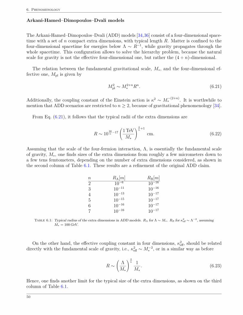
6. Phenomenology
Arkani-Hamed–Dimopoulos–Dvali models
The Arkani-Hamed–Dimopoulos–Dvali (ADD) models [34,36] consist of a four-dimensional space-time with a set of n compact extra dimensions, with typical length R. Matter is confined to thefour-dimensional spacetime for energies below Λ ∼ R−1, while gravity propagates through thewhole spacetime. This configuration allows to solve the hierarchy problem, because the naturalscale for gravity is not the effective four-dimensional one, but rather the (4 + n)-dimensional.
The relation between the fundamental gravitational scale, M∗, and the four-dimensional ef-fective one, Mpl is given by
M2pl ∼M2+n
∗ Rn. (6.21)
Additionally, the coupling constant of the Einstein action is κ2 ∼ M−(2+n)∗ . It is worthwhile to
mention that ADD scenarios are restricted to n ≥ 2, because of gravitational phenomenology [34].
From Eq. (6.21), it follows that the typical radii of the extra dimensions are
R ∼ 10 30n−17
(1 TeVM∗
) 2n
+1
cm. (6.22)
Assuming that the scale of the four-fermion interaction, Λ, is essentially the fundamental scaleof gravity, M∗, one finds sizes of the extra dimensions from roughly a few micrometers down toa few tens femtometers, depending on the number of extra dimensions considered, as shown inthe second column of Table 6.1. These results are a refinement of the original ADD claim.
n RA[m] RB[m]2 10−6 10−16
3 10−11 10−16
4 10−13 10−17
5 10−15 10−17
6 10−16 10−17
7 10−16 10−17
Table 6.1: Typical radius of the extra dimensions in ADD models. RA for Λ ∼M∗. RB for κ2eff ∼ Λ−2, assuming
M∗ = 100 GeV.
On the other hand, the effective coupling constant in four dimensions, κ2eff, should be related
directly with the fundamental scale of gravity, i.e., κ2eff ∼M−2
∗ , or in a similar way as before
R ∼(
ΛM∗
) 2n 1M∗
. (6.23)
Hence, one finds another limit for the typical size of the extra dimensions, as shown on the thirdcolumn of Table 6.1.
50
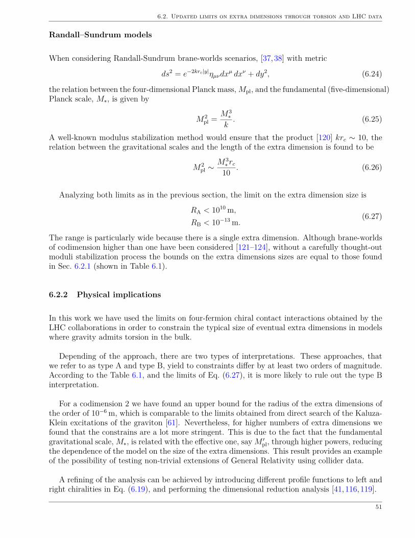
6.2. Updated limits on extra dimensions through torsion and LHC data
Randall–Sundrum models
When considering Randall-Sundrum brane-worlds scenarios, [37,38] with metric
ds2 = e−2krc|y|ηµνdxµ dxν + dy2, (6.24)
the relation between the four-dimensional Planck mass, Mpl, and the fundamental (five-dimensional)Planck scale, M∗, is given by
M2pl = M3
∗k. (6.25)
A well-known modulus stabilization method would ensure that the product [120] krc ∼ 10, therelation between the gravitational scales and the length of the extra dimension is found to be
M2pl ∼
M3∗ rc
10 . (6.26)
Analyzing both limits as in the previous section, the limit on the extra dimension size is
RA < 1010 m,RB < 10−13 m.
(6.27)
The range is particularly wide because there is a single extra dimension. Although brane-worldsof codimension higher than one have been considered [121–124], without a carefully thought-outmoduli stabilization process the bounds on the extra dimensions sizes are equal to those foundin Sec. 6.2.1 (shown in Table 6.1).
6.2.2 Physical implications
In this work we have used the limits on four-fermion chiral contact interactions obtained by theLHC collaborations in order to constrain the typical size of eventual extra dimensions in modelswhere gravity admits torsion in the bulk.
Depending of the approach, there are two types of interpretations. These approaches, thatwe refer to as type A and type B, yield to constraints differ by at least two orders of magnitude.According to the Table 6.1, and the limits of Eq. (6.27), it is more likely to rule out the type Binterpretation.
For a codimension 2 we have found an upper bound for the radius of the extra dimensions ofthe order of 10−6 m, which is comparable to the limits obtained from direct search of the Kaluza-Klein excitations of the graviton [61]. Nevertheless, for higher numbers of extra dimensions wefound that the constrains are a lot more stringent. This is due to the fact that the fundamentalgravitational scale, M∗, is related with the effective one, say M ′
pl, through higher powers, reducingthe dependence of the model on the size of the extra dimensions. This result provides an exampleof the possibility of testing non-trivial extensions of General Relativity using collider data.
A refining of the analysis can be achieved by introducing different profile functions to left andright chiralities in Eq. (6.19), and performing the dimensional reduction analysis [41, 116,119].
51
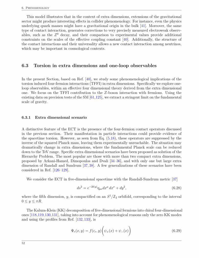
6. Phenomenology
This model illustrates that in the context of extra dimensions, extensions of the gravitationalsector might produce interesting effects in collider phenomenology. For instance, even the physicsunderlying quark masses might have a gravitational origin in the bulk [41]. Moreover, the sametype of contact interaction, generates corrections to very precisely measured electroweak observ-ables, such as the Z0 decay, and their comparison to experimental values provide additionalconstraints on the scales of the effective coupling constant [40]. Additionally, the structure ofthe contact interactions and their universality allows a new contact interaction among neutrinos,which may be important in cosmological contexts.
6.3 Torsion in extra dimensions and one-loop observables
In the present Section, based on Ref. [40], we study some phenomenological implications of thetorsion induced four-fermion interactions (TFFI) in extra dimensions. Specifically we explore one-loop observables, within an effective four dimensional theory derived from the extra dimensionalone. We focus on the TFFI contribution to the Z-boson interaction with fermions. Using theexisting data on precision tests of the SM [61,125], we extract a stringent limit on the fundamentalscale of gravity.
6.3.1 Extra dimensional scenario
A distinctive feature of the ECT is the presence of the four-fermion contact operators discussedin the previous section. Their manifestation in particle interactions could provide evidence ofthe spacetime torsion. However, as seen from Eq. (5.18), these operators are suppressed by theinverse of the squared Planck mass, leaving them experimentally unreachable. The situation maydramatically change in extra dimensions, where the fundamental Planck scale can be reduceddown to the TeV range. Specific extra dimensional scenarios have been proposed as solution of theHierarchy Problem. The most popular are those with more than two compact extra dimensions,proposed by Arkani-Hamed, Dimopoulos and Dvali [34–36], and with only one but large extradimension of Randall and Sundrum [37, 38]. A few generalizations of these scenarios have beenconsidered in Ref. [126–129].
We consider the ECT in five-dimensional spacetime with the Randall-Sundrum metric [37]
ds2 = e−2k|y|ηµνdxµ dxν + dy2, (6.28)
where the fifth dimension, y, is compactified on an S1/Z2 orbifold, corresponding to the interval0 ≤ y ≤ πR.
The Kaluza-Klein (KK) decomposition of five-dimensional fermions into chiral four-dimensionalones [118,119,130,131], taking into account for phenomenological reasons only the zero KK modesand using the profiles from Ref. [132,133], is
Ψr(x, y) = f(cr, y)(ψ+(x) + ψ−(x)
)(6.29)
52
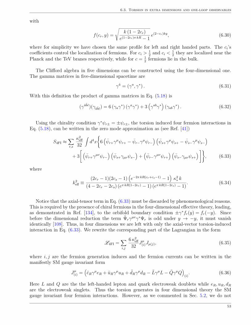
6.3. Torsion in extra dimensions and one-loop observables
with
f(cr, y) =√
k (1− 2cr)e(1−2cr)π kR − 1 e
(2−cr)ky, (6.30)
where for simplicity we have chosen the same profile for left and right handed parts. The ci’scoefficients control the localization of fermions. For ci > 1
2 and ci < 12 they are localized near the
Planck and the TeV branes respectively, while for c = 12 fermions lie in the bulk.
The Clifford algebra in five dimensions can be constructed using the four-dimensional one.The gamma matrices in five-dimensional spacetime are
γa = (γa, γ∗) . (6.31)
With this definition the product of gamma matrices in Eq. (5.18) is
(γabc)(γabc) = 6 (γaγ∗) (γaγ∗) + 3(γabγ∗
)(γabγ∗) . (6.32)
Using the chirality condition γ∗ψr± = ±ψr±, the torsion induced four fermion interactions inEq. (5.18), can be written in the zero mode approximation as (see Ref. [41])
S4FI ≈∑r,s
κ2eff
32
∫d4x
6(ψr+γ
µψr+ − ψr−γµψr−) (ψs+γ
µψs+ − ψs−γµψs−)
+ 3[ (ψr+γ
µνψr−) (ψs+γµνψs−
)+(ψr−γ
µνψr+) (ψs−γµνψs+
) ], (6.33)
where
k2eff ≡
(2cr − 1)(2cs − 1)(e−2π kR(cr+cs−1) − 1
)κ2∗ k
(4− 2cr − 2cs) (eπ kR(1−2cr) − 1) (eπ kR(1−2cs) − 1) . (6.34)
Notice that the axial-tensor term in Eq. (6.33) must be discarded by phenomenological reasons.This is required by the presence of chiral fermions in the four-dimensional effective theory, leading,as demonstrated in Ref. [134], to the orbifold boundary condition ±γ∗fr(y) = fr(−y). Sincebefore the dimensional reduction the term Ψrγ
µνγ∗Ψr is odd under y → −y, it must vanishidentically [108]. Thus, in four dimensions we are left with only the axial-vector torsion-inducedinteraction in Eq. (6.33). We rewrite the corresponding part of the Lagrangian in the form
L4FI =∑i,j
6κ2eff
32 Jµ(i)Jµ(j), (6.35)
where i, j are the fermion generation induces and the fermion currents can be written in themanifestly SM gauge invariant form
Jµ(i) =(eRγ
µeR + uRγµuR + dRγ
µdR − LγµL− QγµQ)
(i). (6.36)
Here L and Q are the the left-handed lepton and quark electroweak doublets while eR, uR, dRare the electroweak singlets. Thus the torsion generates in four dimensional theory the SMgauge invariant four fermion interactions. However, as we commented in Sec. 5.2, we do not
53
6. Phenomenology
consider the complete implementation of the SM gauge symmetry to the gravity framework inquestion. Rather, we adopt here the low energy approach dealing with the broken phase ofthe SM symmetry, taking into account only the known SM fermions specified in Eq. (6.36) withmeasured values of their masses and participating in the SM interactions plus the torsion inducedinteractions in Eq. (6.35).
Using the definitions κ2eff ≡ M−2
Pl and κ2∗ ≡ M−3
∗ and the stabilization value kR ∼ 10 (seeRef. [120]), we obtain
M2Pl ≈
5× 10⁻²⁷M3∗k
; cr ' cs ' 0
10−24M3∗k
; cr ' cs ' 1/2
10−2M3∗k
; cr ' cs ' 1
(6.37)
Let us note that in the following, the effects of curvature in the effective theory in fourdimensions will be ignored, due to the fact that the Universe is essentially flat, cf. Ref. [135].This fact has been used before in Refs. [93, 106, 136], and allows us to discriminate between theEHT and the ECT of gravity. Moreover, this condition is compatible with the independence ofthe Riemaniann curvature and torsion.
6.3.2 Constraints from precision measurements of Z boson decay
Here we analyze the contribution of the torsion induced interactions to the one-loop form fac-tors of the gauge bosons trilinear couplings to leptons. Considering that the gauge sectorof the SM is torsion free, the only effect of torsion comes through the four-fermion contact(axial-vector)⊗(axial-vector) terms in Eq. (6.33).
The neutral gauge boson-fermion vertex
Vµ(k)
f(p)
f(p′)
= ıe Vµ(k)Jµ(p, p′) (6.38)
where Vµ = γµ, Z0µ can be generically parametrized in terms of the fermion neutral current Jµ
form factors FI as
Jµ(p, p′) ≡ u(p′)γµ FV (k2) + FA(k2)γµγ∗ + i
σµν kν2mf
FM(k2) + FD(k2) 12mf
σµνγ∗kν
v(p). (6.39)
We decompose the form factors into the tree level and one-loop contributions Fi(k2) = F treei +
δFi(k2). The tree-level part F treei corresponds to the usual SM couplings of photon or Z-boson to
the fermions, while the one-loop term δFi(k2) may also receive contributions from beyond the SMinteractions. In our case they are the torsion induced four-fermion interactions, aka Eq. (6.33).
54
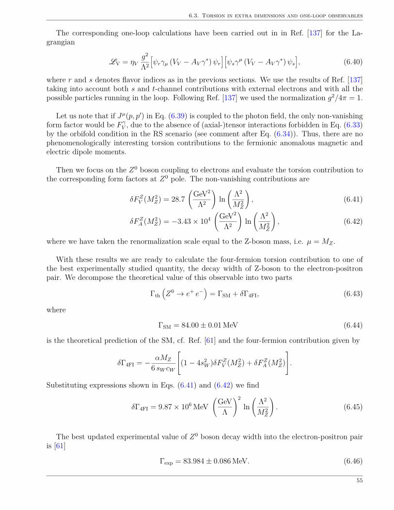
6.3. Torsion in extra dimensions and one-loop observables
The corresponding one-loop calculations have been carried out in in Ref. [137] for the La-grangian
LV = ηVg2
Λ2
[ψrγµ (VV − AV γ∗)ψr
][ψsγ
µ (VV − AV γ∗)ψs], (6.40)
where r and s denotes flavor indices as in the previous sections. We use the results of Ref. [137]taking into account both s and t-channel contributions with external electrons and with all thepossible particles running in the loop. Following Ref. [137] we used the normalization g2/4π = 1.
Let us note that if Jµ(p, p′) in Eq. (6.39) is coupled to the photon field, the only non-vanishingform factor would be F γ
V , due to the absence of (axial-)tensor interactions forbidden in Eq. (6.33)by the orbifold condition in the RS scenario (see comment after Eq. (6.34)). Thus, there are nophenomenologically interesting torsion contributions to the fermionic anomalous magnetic andelectric dipole moments.
Then we focus on the Z0 boson coupling to electrons and evaluate the torsion contribution tothe corresponding form factors at Z0 pole. The non-vanishing contributions are
δFZV (M2
Z) = 28.7(
GeV2
Λ2
)ln(
Λ2
M2Z
), (6.41)
δFZA (M2
Z) = −3.43× 10⁴(
GeV2
Λ2
)ln(
Λ2
M2Z
), (6.42)
where we have taken the renormalization scale equal to the Z-boson mass, i.e. µ = MZ .
With these results we are ready to calculate the four-fermion torsion contribution to one ofthe best experimentally studied quantity, the decay width of Z-boson to the electron-positronpair. We decompose the theoretical value of this observable into two parts
Γth(Z0 → e+ e−
)= ΓSM + δΓ4FI, (6.43)
where
ΓSM = 84.00± 0.01 MeV (6.44)
is the theoretical prediction of the SM, cf. Ref. [61] and the four-fermion contribution given by
δΓ4FI = − αMZ
6 sW cW
(1− 4s2W )δFZ
V (M2Z) + δFZ
A (M2Z).
Substituting expressions shown in Eqs. (6.41) and (6.42) we find
δΓ4FI = 9.87× 10⁶ MeV(
GeVΛ
)2
ln(
Λ2
M2Z
). (6.45)
The best updated experimental value of Z0 boson decay width into the electron-positron pairis [61]
Γexp = 83.984± 0.086 MeV. (6.46)
55
6. Phenomenology
Below we denote the standard experimental deviation from the best fit value as ∆exp = 0.086MeV. We require that the SM contribution taken together with the torsion one be compatiblewith the experimental data (6.46). This leads to the condition
|Γth − Γexp| ≤ α∆exp, (6.47)with the statistical factor α = 1.64 for the 95% C.L. limits, cf. Ref. [61]. Here Γth is defined inEq. (6.43).
In Fig. 6.1, the solid line shows the dependence of the four-fermion contribution δΓ4FI to theZ0 boson decay width on the scale Λ.
102 103 104 105 106
0
1
2
3
4
·10−5
Λ [GeV]
δΓ4F
I[M
eV]
Variation of Z Width Decay
2.5 3 3.5·104
1
1.5
2·10−8
Figure 6.1: The solid line shows the dependence of the four-fermion contribution δΓ4FI to the Z0 boson decaywidth on the scale Λ. The dashed and dotted horizontal lines depict the uncertainty of the SMprediction in Eq. (6.44), and their intersection with the solid curve give bounds on Λ, shown asvertical straight lines on the zoomed part of the plot.
Solving Eq. (6.47) we findΛ ≥ 31.6 (25.8) TeV at 95%C.L., (6.48)
depending on which sign is taken for the uncertainty of the SM prediction in Eq. (6.44). Thesetwo options are depicted in the figure by the dashed and dotted horizontal lines, respectively.
Comparing with the coupling of the contact interaction in Eq. (6.35) with the one in Eq. (6.40),632 κ
2eff ←→
1Λ2 . (6.49)
To solve the Hierarchy Problem in the RS scenario, the value M∗ ∼ 1 TeV has been fixed. Usingthe stabilization value kR ∼ 10 (see Ref. [120]), one obtains the following 95% C.L. limits on thecompactification radius for different fermion localization values,
R .
7.5 (4.9) 1010 m; ci ' 03.7 (2.5) 108 m; ci ' 1/23.7 (2.5) 10−14 m; ci ' 1
(6.50)
56
6.4. Axions in gravity with torsion
where the strongest limit comes from fermions localized near to the Planck brane, which wasexpected due the enhancement of the gravitational scale close to this brane.
6.3.3 Physical implications
In this paper we have considered Dirac fermions coupled with the (minimal) Einstein-CartanTheory of gravity. Within this framework, a four-fermion contact interaction arises, which pre-serves lepton number and fermions are paired by flavor. For this minimal generalization of theEinstein-Hilbert Theory of gravity, the new fermion interaction is suppressed by the gravitationalscale, which in four dimensions is the Planck mass, MPl ∼ 1019 GeV.
In order to circumvent this suppression, the gravitational scale should be much lower, not toofar from the electroweak scale. This is also suggested by the arguments of radiative stability ofthe Higgs boson mass. We considered the Randall-Sundrum scenario which does not suffer of theproblems of hierarchical scales. It suggests the existence of one large extra dimension compactifiedon a S1/Z2 orbifold, and a fundamental gravitational scale (M∗), which gives rise to an effective(exponentially enhanced) Planck mass through a dimensional reduction. We implemented thetorsional gravity into this scenario.
The four-fermion interaction in five-dimensions yields both axial-vector and (axial-)tensorinteractions. Interestingly, the orbifold structure of the extra dimension in RS scenarios requiresvanishing the (axial-)tensor terms, for the effective four-dimensional theory to contain chiralfermions. For this reason there are no phenomenologically meaningful torsion contributions tothe fermionic anomalous magnetic and electric dipole moments.
On the other hand the remaining (axial-vector)⊗(axial-vector) torsion induced interactionsgive a contribution to the width of Z0 → e+e−, which allowed us to extract from the existingexperimental data upper limits on the compactification radius in the RS setup. These limitsshown in Eq. (6.50) are more stringent then the corresponding limits previously derived in theliterature (see, for instance, Ref. [39] and references therein).
Note that these limits are not going to change even after the complete implementation of theSM gauge symmetry in the ECT gravity framework, not considered in the present work. This isbecause the only phenomenologically relevant remnant of of the ECT, the torsion induced fourfermion interaction in Eq. (6.35), is already SM gauge invariant.
6.4 Axions in gravity with torsion
The recent discovery of the Higgs-like boson has completed the list of the Standard Model (SM)particles, and therefore has confirmed this as the current framework for particle physics. However,it is well-known that the SM suffers from various internal problems indicating that this is not afundamental theory, and in fact it should be considered just as an effective low energy theory.The strong CP-problem is one of these problems. It emerges from adding to the QCD Lagrangianthe so called θ-term
L ⊃ − θ αs2π Tr (GG) , (6.51)
57
6. Phenomenology
written in terms of the QCD gluon field strength 2-form G. This is a renormalizable and gaugeinvariant term, which violates CP and it is allowed in any generic gauge theory in four dimensions.In the SM it contributes to CP-odd observables such as the neutron electric dipole moment,which is stringently constrained by experiment, pushing the θ-parameter down to 10−10. Sincethe natural value of this parameter should be of order one, this becomes a fine tuning problem.The question of why it turns out to be so small is the strong CP-problem.
A solution of the strong CP-problem has been found by Peccei and Quinn (PQ) in the periodic-ity of the non-perturbative QCD θ-vacuum [138,139] by promoting the θ-parameter in Eq. (6.51)to be a field θ(x). This can be done by means of a pseudoscalar field, φ(x), of any origin, coupledto the Pontryagin density of the gluon field, i.e.
L = −αs2π θ(x) Tr (GG) , (6.52)
where θ(x) = θ+φ(x)/fφ and fφ the decay constant of φ(x). Thus, the interaction θ(x) Tr (GG)generates in the θ-vacuum a non-trivial potential for θ(x), selecting a zero vacuum expectationvalue 〈θ〉 = 0, corresponding to 〈φ〉 = −θfφ. The fluctuations around this vacuum, φ(x) = 〈φ〉+a(x), generates a pseudoscalar field a(x), dubbed the “axion”. Then dynamically the CP-violatingterm (6.51) is replaced by the CP-conserving interaction a(x) Tr (GG). This pseudoscalar fieldcould be a Goldstone boson of a U(1)A symmetry as was proposed in Refs. [138,139]. Nevertheless,its spontaneous symmetry breaking scale has to be much larger than the electroweak scale, to becompatible with the experimental data as well as with astrophysics and cosmology7. There aremany symmetry based proposals of this kind in the literature, as possible solutions of the strongCP-problem (for a recent review see Ref. [140]). A characteristic feature of this approach is thatall the couplings of the axion are determined by the scale of symmetry breaking, which is a freeparameter.
On the other hand it is well-known that various scenarios for the Planckian physics involveaxion-like fields [141–144]. Those fields can play the same role as the conventional Goldstonetype axions in the solution of the strong CP-problem, but with all their couplings completelydetermined by the Planck scale.
In particular the axion-like fields may appear rather naturally in a field theory on the torsionfulmanifolds, with its metric sector treated as a “rigid” background. The first scenario of this kindwas proposed in Ref. [145], where an axion-like field appears as a consequence of the constraintimposed on the quantum theory, requiring the conservation of the torsion charge, as suggestedby the classical theory.
Recently, in Ref. [146], the axion has been introduced as a pseudoscalar field, the so calledBarbero–Immirzi (BI) axion, interacting with gravity via the Nieh–Yan density [101, 147–149].One of the motivations for the introduction of this field was the possibility of eliminating theconfusing divergence present in the U(1)A rotated fermion measure of the Euclidean path integralon the manifolds with torsion. In addition to the usual Pontryagin density, in this case thereappears a Nieh-Yan term, which becomes divergent when the regularization is removed [150].The significance of this divergence was debated in the literature [151,152] and a consensus on itsstatus has not yet been reached. In the model of Ref. [146] this divergence can be absorbed bya redefinition of the Barbero–Immirzi field. This axion-like field was also proposed in Ref. [153],
7This fact ruled out the PQ axion, since the spontaneous symmetry breaking scale of the U(1)A symmetry proposed in Refs. [138,139], was the EW one, i.e. ΛEW ∼ 246 GeV.
58
6.4. Axions in gravity with torsion
in order to solve the strong CP-problem in the Peccei–Quinn spirit.
In the present Section, we show that the conservation of the torsion charge, within the frame-work of Ref. [145], is equivalent to demanding a vanishing Nieh–Yan density. This constraintcan be implemented into the quantum theory by means of a Lagrange multiplier, identified withthe so-called the Kalb-Ramond (KR) axion [154], due to its similararity with the axion-like fieldcoming from string theory.
Despite the starting points of Refs. [145] and [146] seem to be different, they have the samephysical properties when the torsion is integrated out. Therefore, within the effective theory,the Kalb–Ramond [154] and the Barbero–Immirzi [146] axions are equivalent. We rigorouslydemonstrate this equivalence and study the solution of the strong CP problem based on thesetorsion descended (TD) axions. Then we examine their possible cosmological and astrophysicalimplications.
We concentrate on the discussion of axions in Einstein-Cartan theory of gravity with torsion.For discussions on the role of axions motivated by Chern-Simons-type terms, see Ref. [155], whereas a cosmological application, the accelerated expansion of the Universe has been considered [155,156].
6.4.1 Classical gravity setup
We consider the ECT of gravity coupled with fermions in 4-dimensions, as a particular case ofthe theory described on Sec. 5.3. In terms of differential forms, the gravitational action can bewritten as
Sgr = 14κ2
∫εabcdRab ec ed , (6.53)
where κ is related with the Newton’s constant GN through κ2 = 8πGN .
In the following the fields of the SM are assumed to live in a curved torsionful spacetime. Thenontrivial coupling of matter with torsion enters in the fermionic sector through the covariantderivative,
Dψ = dψ + 14ω
abγabψ + ıgAψ + ıeBψ , (6.54)
where A and B denote the SU(3) and U(1) gauge bosons 1-forms respectively. Therefore, thecomplete model is described by the action
S = Sgr −12∑f
∫ (ψfγ ?Dψ −Dψf ? γψf
)− 1
2
∫F ? F −
∫Tr [G ?G] , (6.55)
where ψ = −ıψ†γ0 is the usual Dirac adjoint, γ = γaea and the subscript f indicates the SMfermion species. The symbol ? denotes Hodge duality, while G and F are the SU(3)C and U(1)emgauge field strength 2-forms, respectively.
When the action in Eq. (6.55) is varied with respect to the vierbein, one obtains the corre-sponding Einstein-Cartan equation of motion
Rab −12ηabR = κ2τab , (6.56)
59
6. Phenomenology
where τab is the energy-momentum tensor of the system. In its form, this equation looks sim-ilar to the Einstein’s equation derived within General Relativity. However, as was stated inChap. 5, the two equations are different in general, because the presence of torsion gives rise toan antisymmetric part in both sides of the equation.
On the other hand, the second equation of motion can be obtained varying the action inEq. (6.55) with respect to the Lorentz connection. Furthermore, such equation implies Tdmm = 0,which means that the torsion tensor is completely antisymmetric and, therefore, there is no contri-bution in this theory coming from the coupling of the torsion trace with the vectorial fermioniccurrent. Additionally, using the identity γa, γbc = 2 ı εabcd γd γ∗, where γ∗ ≡ ı γ0γ1γ2γ3, theequation of motion for the Lorentz connection is nothing but an algebraic equation for the tor-sion tensor
Tabc = −κ2
2∑i
εabcdJ∗di = 2Kabc (6.57)
where J∗di ≡ ı ψiγdγ∗ψi. Moreover, in light of the Eq. (6.57), the only contribution of the torsion,
comes from its axial irreducible component. Therefore, it is convenient to work with the followingdefinition
S = ?T = 13!εabcdT
abced , (6.58)
where T = 1/3!Tabc ea eb ec and S = 1/3! εabcd Tabc ed denotes 3-form torsion and 1-form axial com-ponent respectively.
Now we rewrite Eq. (6.55), showing explicitly only those terms which depend on the torsionaxial component
S = S0 + 34κ2
∫S ? S − 3
4
∫J∗ ? S, (6.59)
where S0 = Sgr + Sψ +Sgk with Sgk representing the gauge field kinetic terms (the last two termsin Eq. (6.55)). The entity J∗ = ∑
f (J∗f )aea denotes the axial current 1-form, where the sum runsfor all the fermionic flavors f .
6.4.2 Quantum theory and torsion-descended axion
The quantization of the model with the action given in Eq. (6.59) can be carried out on thebasis of the path integral representation for the generating functional. However, at present it isunknown if this procedure is applicable to the quantization of the whole gravity sector (for thecurrent status of this problem see, for instance Refs. [157,158]).
In the scenario studied here, the SM fields lie on a torsionful manifold, whose only quantumgravity effects enter through the torsion, while the metric or Riemmanian curvature remain asclassical variables. Quantum torsion seems to be easily treatable because the equation of motionfor the torsion (6.57) is algebraic, showing that the torsion is a non-propagating field, which canbe exactly integrated out from the theory.
However, as it was observed in Ref. [145], this treatment of the torsion should be done withcaution. The point is that from Eqs. (6.57) and (6.58) it follows S ∝ J∗. Since the action (6.59)
60
6.4. Axions in gravity with torsion
is U(1)A symmetric, the Nother current J∗ is conserved at classical level, leading, as follows fromthe above relation, to the conservation of the “torsion charge” QS =
∫?S.
On the other hand, we know that the fermionic measure of the path integral is not U(1)Ainvariant. This fact manifests as the anomalous non-conservation of J∗ at the quantum level. Aspointed out in Ref. [145], this must be taken into account before integrating out the torsion, inorder to maintain the self-consistency of the constructed effective theory.
Following Ref. [145], an effective quantum theory can be constructed through a constraintrequiring the conservation of the “torsion charge” d?S = 0. Notice that this is a gauge invariantcondition, which is important for the self-consistency of the SM sector of the theory. Later wewill show that this condition eliminates the divergent part of the U(1)A anomaly, affecting thetractability of the quantum theory in the presence of the torsion.
The quantum generating functional, with this condition incorporated, takes the form
Z =∫ ∏
ϕ
DϕDS eıS[ϕ] δ (d ? S) , (6.60)
where ϕ denotes all the fields except for eaµ, treated as a rigid background. The argument of thedelta in Eq. (6.60) can be passed to the effective action using the integral representation
δ (d ? S) =∫Dφ e
∫ıφd?S =
∫Dφ e−
∫ıdφ ?S . (6.61)
This allows us to write
Z =∫ ∏
ϕ
DϕDφDS eıS[ϕ]−∫ıdφ ?S . (6.62)
However, as the Appendix D shows, it is possible to rewrite the argument of the exponential inEq. (6.62). Thus, since S is a non-propagating field, we can integrate it out in the standard way.As a result we get the effective action
Seff = S0 −3κ2
16
∫J∗ ? J∗ − 1
2
∫dΦ ? dΦ + κ
2
√32
∫Φ d ? J∗ . (6.63)
For convenience we have made a redefinition Φ = κ√
2/3φ. Notice that the integration outof the torsion makes Φ(x) a dynamical field with the canonical kinetic term. As follows fromthe last term in Eq. (6.63) this field is pseudoscalar. It is what we called in the IntroductionKalb-Ramond (KR) axion field.
At the quantum level, the last term of in Eq. (6.63) is nothing but the axial anomaly [159].In the path integral language d ? J∗ 6= 0 is the manifestation of the U(1)A non-invariance of thefermionic measure [160], mentioned at the beginning of this Section.
On the Riemann-Cartan manifolds the axial anomaly was first studied in Refs. [161–163].However, as shown in Ref. [150], the computation of such anomaly gives rise, in general, to anadditional previously missed term, called Nieh-Yan topological density [147]. Therefore, a U(1)A
61
6. Phenomenology
rotation the fermionic measure experiences a non-trivial variation [150]
DψDψ →DψDψ × expı α∫ [
αemQ2
πF F + αsNq
2π Tr [GG] (6.64)
+ Nf
8π2 Rab Rab + 2M2(T a T a − ea eb Rab
) ]. (6.65)
Here αem and αs are the electromagnetic and QCD couplings, respectively, Nf is the total numberof fermionic flavors, Nq is the number of quarks and Q2 = ∑
f Q2f , where Qf is the charge of f
fermionic flavor. The last term in Eq. (6.65) is the Nieh-Yan (NY) topological density with theregulator multiplier divergent when the regularization is removed M →∞. As mentioned before,the status of this divergence is still debated in the literature.
However we find that in the approach of Ref. [145] it is irrelevant since the NY term Nvanishes identically due to the condition d ? S = 0 imposed on quantum theory by insertion ofthe corresponding delta function in Eq. (6.60). In fact this follows from the identity derived inRef. [147]
N ≡ T a T a −Rab ea eb = d (ea T a) , (6.66)and the definition of the field S in Eq. (6.58) written in the form
? S ∝ ea T a. (6.67)
Then from Eqs. (6.66) and (6.67) it follows
d ? S = 0⇒N = 0. (6.68)
Thus, neglecting the Nieh-Yan term in the axial anomaly, we can write for the axial current
d ? J∗ = −αemQ2
πF F − αsNq
2π Tr [GG]− Nf
8π2 Rab
Rab. (6.69)
The right-hand-side is written in terms of torsion-free quantities. This is attainable by theintroduction of proper counterterms, as shown in Refs. [164–169].
Now we substitute the identity (6.69) into Eq. (6.63) and obtain the resulting effective actionof the model
Seff = S0 −1
2f 2Φ
∫J∗ ? J∗ − αemQ
2
πfΦ
∫ΦF F − 1
2
∫dΦ ? dΦ
− 18π2
∫ (Θ + Nf
fΦΦ)
Rab
Rab −αs2π
∫ (θ + Nq
fΦΦ)
Tr [GG] . (6.70)
Here we introduced a parameter
fΦ = κ−1√
8/3 ' 4× 10¹⁸ GeV, (6.71)
analogous to the decay constants of fields with derivative couplings, such as Goldstones of spon-taneously broken symmetries.
In the effective action (6.70) we added the QCD and the gravitational θ- and Θ-terms, re-spectively. They are the gauge and gravitational Pontryagin densities allowed by the gauge
62
6.4. Axions in gravity with torsion
symmetries of the theory. These terms are also needed for the model completeness, and play therole of counterterms for the axial anomaly quantum corrections. They do not affect the previousderivation, since due to their topological nature they do not change the equations of motion.
Recently in Ref. [146] there has been proposed an alternative scenario in gravity with torsionalso leading to an axion-like field. This scenario is inspired, in particular, by the Chern-Simonsmodified gravity motivated in its turn by string theory. The gravitational action according toRef. [146] is modified at the classical level by the term
Stot = S +∫β(x) N , (6.72)
where S is the action given in Eq. (6.59). This action, being used in the quantum generatingfunctional, allows one to absorb the divergent NY part of the anomalous U(1)A variation ofthe fermion measure (6.65) by a renormalization of the field β(x) called in Ref. [146] Barbero-Immirzi (BI) axion. The field β(x) becomes a dynamical field with the canonical kinetic termafter excluding a non-dynamical torsion field using the classical equation of motion
S = 23κ
2dβ + 12κ
2J∗ , (6.73)
derived from the action (6.72). This is equivalent to integrating out the torsion field S in thegenerating functional as was shown in the Appendix D. Note that the field β(x) in the classicalaction (6.72) is nothing but a Lagrange multiplier setting the classical level constraint N = 0.Now one can immediately realize that in a view of the identities (6.66) and (6.67) it is equivalentto the constraint d ? S = 0, which in the approach of Ref. [145] was set at quantum level as aconstraint incorporated in the generating functional (6.60). On the other hand both approacheslead to the same effective quantum theory with the effective action given in Eq. (6.70) with theidentification of the KR and BI axions Φ(x) ≡ β(x).
As we have seen KR and BI axions originate from rather different treatments of quantumtheory in the presence of the torsionful gravity. Nevertheless from the point of view of low-energyeffective theory and the resulting phenomenology they both are equivalent particles, which wecall from now on torsion descended (TD) axions.
Additionally, the TD axions may also appear in the context of the torsion-induced quintessen-tial axions [155]. In this framework, the axial current is modified by the addition of the Chern-Simons-type terms, in order to be conserved in the zero mass limit. The complete cancellationof the torsion sector in the anomaly, can be addressed requiring the torsion to be an exteriorderivative of a pseudoscalar field, identified later with the axion [155]. Remarkably, this approachleads to the same effective theory as Refs. [145] and [146] for a constant dilaton field.
6.4.3 Phenomenology and cosmology with TD axions
In the effective action in Eq. (6.70) of the considered TD axions the last term is the most impor-tant in the context of the strong CP-problem. The presence of the coupling of an axion-like fieldto the gluon field Pontryagin density is the necessary and sufficient condition for the solutionof the strong CP-problem via the Peccei–Quinn mechanism. The TD axion decay constant fΦintroduced in Eq. (6.70) represents a typical energy scale of the model, related to the Planck
63
6. Phenomenology
scale. Thus, the TD axions Φ emerge without any accompanying free parameter. This drasti-cally distinguish them from the axions introduced as Goldstone fields of spontaneously brokensymmetries, requiring at least one free model parameter, i.e., the scale of symmetry breaking.
In principle in certain models both the TD and Goldstone axions can coexist mixing with eachother [153]. We do not consider this case here since in the presence of the TD axions, solving thestrong CP problem without free parameters, introduction of other axions looks excessive.
Focusing on the last term in Eq. (6.70), let us write down, θ(x) = θ + Φ(x)Nq/fΦ. Themain point of the Peccei–Quinn mechanism is that the coupling ∼ ∫ θ(x) Tr [GG] generates anontrivial potential for the θ(x) field. The periodicity of this potential in θ [170] selects theunique nontrivial minimum 〈θ(x)〉 = 0, corresponding to 〈Φ〉 = −θ fΦ/Nq. Perturbations aroundthis vacuum generate the physical pseudoscalar axion field a(x) = Φ(x)− 〈Φ(x)〉. Thus the onlysurviving piece of the last term of Eq. (6.70) is the CP-conserving interaction a(x) Tr [GG]. Thissolves the strong CP-problem with the help of the TD axions. The mass ma of the TD axioncan be calculated in the usual way, as is done for any axion field (for a review c.f. Ref. [171]),and depends only on the parameter fΦ defined in Eq. (6.71). The nontrivial mass is generatedby instantons and for the value in Eq. (6.71) it turns to be
ma ≈ mπfπfΦ
√mumd
mu +md
∼ 10−12 eV, (6.74)
where fπ = 93 MeV is the π-meson decay constant and mπ,mu,d are the masses of π-mesonand u, d- quarks. Such an extremely light particle, having the inverse Planck mass suppressedinteractions with gauge fields, is unobservable in laboratory experiments.
Nonetheless, an axion with these properties may play a significant cosmological and astro-physical role, since it must satisfy the existing limits related to its origins. These aspects of thetorsion-descended axions considered here, have been studied in Ref. [153]. It has been shownthat such axions safely pass all the known astrophysical constraints, which originate from theenergy loss of a stellar core in the form of axions and its impact on stellar evolution.
An interesting cosmological prediction applied to the torsion-descended axions, also discussedin Ref. [153], is the production of axion isocurvature perturbations which amplitude is constrainedfrom the above by WMAP data [172, 173]. Assuming that they are the dominant component ofdark matter in the Universe it was found the upper limit [153]
HI ≤ 1010 GeV , (6.75)
for the Hubble expansion rate HI during inflation. Now we can estimate the tensor-to-scalarratio r = PT/PS using expressions for the power spectra of the scalar PS and tensor PT pertur-bations [174]
PS ≈1
8π2
(H2I
εM2P
), PT ≈
2π2
(H2I
M2P
). (6.76)
Here MPl = 1/√
8πGN ≈ 2.44× 10¹⁸ GeV is the reduced Planck scale and ε is the standard slow-roll parameter. We use the Planck Collaboration result PS ≈ 2.19× 10⁻⁹ (see Refs. [175, 176])and find from Eqs. (6.76)
HI ≈ 2.5× 10¹⁴ GeV√r. (6.77)
64
6.4. Axions in gravity with torsion
Using the limit (6.75) one finds the prediction for the cosmology with torsion-descended axions
r ≤ 1.6× 10⁻⁹. (6.78)
This is in dramatic contradiction with the recently published result by BICEP2 [43], r = 0.2+0.07−0.05.
Nevertheless, the situation has recently changed after the publication of the Planck Collaborationdetailed analysis of the impact of the diffuse Galactic dust polarized emission on the measurementsof the polarization of the CMB [44]. It has been shown that the BICEP2 result can be accountedfor the presence of this dust. Thus, the torsion-descended axions, considered in the present paper,are currently not excluded by the cosmological data. Their cosmological test via the tensor-to-scalar ratio r is postponed for the future. Results of improved measurements of r, taking intoaccount the complications with the diffuse Galactic dust, are expected to come in the near futurefrom the Keck Array [177] and BICEP3 [178] telescopes. The first results of the joint analysisof BICEP2/Keck Array and Planck data has been recently issued [179] showing only an upperlimit r < 0.12 at 95% C.L. New results from BICEP3, which will improve this limit are expectedduring 2015 and 2016 seasons [179].
The following final note might be in order. If the considered scenario is incorporated intothe extra dimensional setup [34, 36–38] amended with the torsion [40, 108] the fundamental D-dimensional Planck scale M∗ could be reduced down to the TeV values, dramatically changingthe phenomenology and cosmology of the TD axions. In fact, making a rescaling MPl → M∗ ≥100 GeV in Eqs. (6.71) and (6.74), we find the values ma ≤ 38 keV and fΦ ≥ 100 GeV. Thenfor the rate of a → γγ we get Γaγγ ≤ 10−16 eV. As to the cosmological aspects of the extradimensional TD axions, they require a dedicated study. In particular, the value of the tensor-to-scalar ratio r cannot be obtained from (6.78) by the simple rescaling of MPl. Let us recallthat the bound in Eq. (6.78) was obtained using the limit (6.75) derived in Ref. [153] with theassumption that the axions be out of thermal equilibrium with photons during inflation. Thiscondition can be violated for the values of Γaγγ given above. The role of the extra dimensionalTD axions as a Dark Matter candidate should also be reconsidered. The corresponding study isin progress and its results will be published elsewhere.
65

6. Phenomenology
66
Chapter 7
Conclusions
In the present thesis, we have explored one of the natural extensions of the (pseudo-)Riemanniangeometry. Such an extension, includes non-vanishing torsion on the manifold. Within this geo-metrical approach, the torsion tensor appears as the non-Riemannian part of the affine connection,because it transforms as a tensor, in contrast to its Riemannian counterpart, which transformsas a connection under diffeomorphisms.
As was proposed by Elie Cartan [21–23], such manifolds are determined by its curvature andtorsion, considered as independent variables. Additionally, those variables are related with thevielbein field, which encondes the information of the metric, and the Lorentz connection whichdetermines how the parallel transport is performed with respect to the local Lorentz group.Following the Cartan first order formalism, the vielbein and the Lorentz connection can betreated as independent variables as well. In such a way, this formalism is more general than GRbecause there is no a priori constraint which relates the metric with the affine connection. Infact, within the formalism used throughout this thesis, they are independent quantities and anyconstraint between them, is just a consequence of the equations of motion.
On the other hand, years after the Utiyama’s proposal [18], the idea of the PGT first developedby Kibble [19] and Sciama [20], exhibits the same geometrical structure of the Riemann-Cartanmanifold. In such a theory, the Lorentz curvature appears as the gauge field strength of thelocal Lorentz transformations while the torsion tensor appears as the gauge field strength oflocal translations. Further, local translations play the role of general coordinate transformations.However, despite the inclusion of an invariant gravitational theory under local translations isstill a pending task, it is possible to identify the Riemann-Cartan geometry as the correct one todevelop the PGT.
Among the possibilities of PGT, the minimal extension towards a torsional theory, the ECTshows an interesting behaviour when it is coupled with fermionic matter [19]. As we saw inChap. 5, both theories, i.e. with or without torsion, are not equivalent from the effective theorypoint of view. In fact, as was pointed out in Sec. 5.3, the ECT coupled with fermions gives riseto a four-fermion interaction, absent in the torsion-free description, and offers a discriminationbetween both theories. Nevertheless, due to its coupling constant in four dimensions, such adifference might be sizeable at the Planck scale. Even though it has been impossible so far toreach those energies at particle accelerators, the cosmological and astrophysical sources couldoffer some insights about it.
However, since the ECT can be extended to D-dimensional spacetimes in a straightforwardway, the torsion induced four-fermion interaction (TIFFI) provides a novel test of such scenarios.
Cristobal Corral 67
7. Conclusions
After the compactification of the extra dimensions, it is possible to obtain a 4-dimensional effec-tive theory, where the information of the extra dimensions is encoded in the coupling constantsof such theory. On the other hand, as we studied in Ref. [39], the ATLAS and CMS analysis ofthe invariant mass and dijet’s angular distribution of pp collisions at
√s = 7 TeV, can be used
to constrain the coupling constant of such a four-fermion interactions. Further, using the resultsof ATLAS and CMS collaborations, together with a non-hierarchical choice of the fundamentalscale of gravity, we extracted limits for the size of the extra dimensions in both ADD and RSscenarios. Interestingly enough is the case for D = 4 + n, with n > 2, because the limits aremuch more stringent as we can see from the Table 6.1.
As was pointed in Ref. [40], the TIFFI might have an impact on the one-loop observables atlow energies. Within this framework, we derived an effective theory in four dimensions comingfrom the RS scenario with 1 warped extra dimension. In such an effective theory, we calculatedthe contribution of torsion to the one-loop form factors of the vector-fermion-fermion operator.With them, we calculated the contribution of the TIFFI to the Z boson decay width. Usingthe updated data of the precision measurements of this decay, we were able to constrain thefundamental scale of gravity, and therefore the size of the extra dimensions, twice better than inRef. [39]. Additionally, we looked for further contributions to physical observables, such as theleptonic anomalous magnetic moment. However, since the RS model is compactified on a S1/Z2orbifold, its structure annihilates the (tensor) ⊗ (tensor) component of the TIFFI. Hence, thereis no contribution to neither the magnetic form factor nor to the leptonic anomalous magneticmoment.
In Ref. [41], we have argued that the mechanism for the EWSB, proposed by Burdman andDa Rold [90], appears in a natural way within the context of ECT coupled with fermions. Here,the Yukawa sector arises through the TIFFI, after the condensation of a fourth family of heavyquarks. Such a condensate, acts as a composite Higgs boson, similar to technicolor theories. Inthis context, fermions aquire mass through the Yukawa sector, generated dynamically within themodel. Additionally, they receive contributions coming from the fermionic Kaluza-Klein toweras well. However, due to the special kind of interaction induced by torsion, the effective massmatrix is diagonal and this model does not possess the richness of Ref. [90] about the quarkmixing. Nevertheless, it gives a natural hierarchy of the quark masses as a consequence of thecompactification.
As we saw in the Sec. 5.2, gauge fields does not minimally couple to torsion within the firstorder formalism. This fact ensures that the inclusion of gauge symmetries is not violated in theRiemann-Cartan manifolds. Thus, we have included the SU(3) and U(1) gauge symmetries inRef. [42]. In this context, we considered a solution of the strong CP problem via the Peccei–Quinn mechanism, implemented into the theory of gravity with torsion. We showed that theself-consistency condition of quantum theory d?S = 0 proposed in Ref. [145] is equivalent to therequirement of vanishing Nieh–Yan topological density on the spacetime manifold. The Lagrangemultiplier field, incorporating this constraint, leads to the torsion-descended axion coupled tothe gluon Pontryagin density, Tr [GG], and therefore, allows application of the Peccei–Quinnmechanism for solving the strong CP problem.
We considered the Kalb–Ramond and the Barbero–Immirzi axions proposed in the literaturefrom quite different theoretical perspectives. We found that from the view point of the effectivetheory these two torsion-descended axions are equivalent.
68
.
An important property of the torsion-descended axions is that their phenomenology has no freeparameters being completely determined by the Planck scale or, equivalently, by the Newton’sgravity constant. The torsion-descended axion masses and their characteristic “decay” constants,are extremely small due to the Planck suppression, typical for this family of axions rooted ingravity. We demonstrated the compatibility of the torsion-descended axions with all the existingcosmological and astrophysical limitations, as well as prospects for testing them in the nearfuture measurements of the tensor-to-scalar ratio of the perturbation modes of the CMB. Wealso estimated the possible role of extra dimensions in phenomenology and cosmology of torsion-descended axions.
Summarizing, the theory studied in this thesis is one of the natural candidates for theoriesbeyond GR. This theory is both local Lorentz and diffeomorphism invariant, it respects the gaugesymmetries and reproduces the GR in the limit of vanishing torsion, and couples fermions togravity in a natural way. Since the SM fields are included together with gravity it was importantto engage the vielbein formalism. Finally, ECT is phenomenologically different from the GR.Such differences might have an impact (or not) on either the extra dimensional scenarios or inthe high energy regime. The eventual measure of those deviations, can be used to verify or ruledout the ECT.
69
7. Conclusions
70
Appendix A
The Contorsion Tensor
Let us consider the metricity condition
∇µgνλ = ∂µgνλ − Γµκνgκλ − Γµκλgνκ = 0, (A.1)
which guarantees that lenghts and angles are preserved under parallel transport along any curve.Further, after two cyclic permutation of the indices on Eq. (A.1), one obtain two extra equations
∂µgνλ − Γµκνgκλ − Γµκλgνκ = 0, (A.2)∂λgµν − Γλκµgκν − Γλκνgµκ = 0, (A.3)∂νgλµ − Γνκλgκµ − Γνκµgλκ = 0. (A.4)
Adding, Eq. (A.2) + Eq. (A.4) - Eq. (A.3), one gets
∂µgνλ + ∂νgνµ − ∂λgµν − Γµκνgκλ − Γµκλgνκ − Γνκλgκµ − Γνκµgλκ + Γλκµgκν + Γλκνgµκ = 0.(A.5)
In general, the affine connection can be splitted into its symmetric and an antisymmetric part as
Γµλν = Γ(µλν) + Γ[µ
λν]. (A.6)
Using the latter decomposition and replacing it back into Eq. (A.5) one obtains
∂µgνλ + ∂νgνµ − ∂λgµν − 2Γ(µκν)gκλ − 2Γ[λ
κµ]gκν − 2Γ[ν
κλ]gκµ = 0. (A.7)
Now, the antisymmetric part of the connection, is identified with the torsion tensor, and one candefine it via 2Γ[µ
κν] ≡ Tµκν . Solving for the symmetric part, we get
Γ(µρν) = 1
2gλρ (∂µgνλ + ∂νgνµ − ∂λgµν) + 1
2 (T ρµν + T ρνµ) , (A.8)
= µρν+ 12 (T ρµν + T ρνµ) , (A.9)
where µρν are the usual Christoffel symbols used in GR, and the indices are lowered and/orraised using the metric gµν . Using this last result, and inserting it into the decomposition (A.6),we get
Γµκν = µκν+ 12 (Tµκν + T κµν + T κνµ) , (A.10)
≡ µκν+Kµκν , (A.11)
where, we have define the Contorsion Tensor via Kµκν ≡ 12 (Tµκν + T κµν + T κνµ), and this part
of the affine connection transform as a tensor under diffeomorphisms, unlike the Riemmanianpart of the connnection, which transform as a connection.
Cristobal Corral 71
A. The Contorsion Tensor
72
Appendix B
SU(N) identities
Let us consider some SU(N) transformation
U (θ) = ei θA TA , (B.1)
where TA are generators of the Lie algebra associated to the SU(N) Lie group and θ is some realinfinitesimal parameter. These generators are hermitian (T †A = TA), traceless (Tr [TA] = 0) andthey satisfy the following (anti-)commutation relations
[TA, TB] = TATB − TBTA = i fABC TC (B.2)
TA, TB = TATB + TBTA = 1NδAB 1N×N + dAB
C TC (B.3)
where fABC ∈ R1 are the structure constants which are antisymmetric in A,B due to the commu-tator in Eq. (B.2). The constants dABC ∈ R1 are completely symmetric. Adding both equationsand applying trace on both sides we obtain
Tr [TATB] = 12δAB. (B.4)
Using the SU(N) transformation acting on some representation of the group, is easy to notethat 1, TA form a basis. Then one it is possible to expand any N × N matrix representationin terms of such a basis
M = a 1N×N + bA TA. (B.5)The coefficient a can be easily obtained applying trace on both sides. The coefficients bA can beobtained multiplying on both sides by TB and then applying trace. With this we get a = 1
NTr [M ]
and bA = 2 Tr[M TA
]. Then, it is easy to write (in components)
Mij = 1NM l
l δij + 2Mmn
(TA)n
m
(TA)ij. (B.6)
Using Mij = Mmnδmiδ
nj , M l
l = Mmm = Mm
nδnm and considering some arbitrary Mm
n one arrivesto the useful identity
δimδjn = 1Nδijδmn + 2
(TA)ij
(TA)mn. (B.7)
For instance, in the SU(2) case, one possible choice for the generators of the Lie algebra arethe Pauli matrices, this means that TA = 1
2σA where A = 1, 2, 3. With this, the Eq. (B.7) reads
δimδjn = 12 δijδmn + 1
2(σA)ij
(σA)mn. (B.8)
Cristobal Corral 73
B. SU(N) identities
Other interesting example is the SU(3) case where the common choice for their generators arethe Gell-Mann matrices, this means that TA = 1
2λA where A = 1, . . . , 8. With this, the Eq. (B.7)
reads
δimδjn = 13 δijδmn + 1
2(λA)ij
(λA)mn. (B.9)
74
Appendix C
Real Dirac Action with Torsion
In this appendix we will demonstrate that, in general, the Hermitian Dirac action in torsionfulmanifolds differs from the usual one. They will give the same description if and only if the traceof the torsion tensor vanishes, otherwise there appears an extra interaction between the torsiontrace and the fermionic vector current and, therefore, both actions are no longer equivalent.
C.1 Partial integration in spacetimes with torsion
In field theory, we often argue that the boundary term∫dDx ∂µV
µ, does not contribute to theequations of motion as soon as the vector field V µ(x) vanishes at large distances. Additionally,there exist a similar relation in curved spacetimes for the Levi-Civita connection, i.e.∫
dDx√−g ∇µV
µ =∫dDx ∂µ
(√−g V µ), (C.1)
where we have used the identity
∇µVµ = 1√−g∂µ
(√−g V µ). (C.2)
However, in spacetime with nonvanishing torsion there appears an extra contribution comingfrom the torsion sector. Let us consider the torsionful covariant divergence
∇µVµ = ∂µV
µ + Γµµλ V λ = ∂µVµ +
(Γµµλ +Kµµλ
)V λ = ∇µV
µ − Tλ V λ, (C.3)
where in the last equality we have used the identity Kµµλ = −Tλµµ ≡ −Tλ. Therefore, the partialintegration using a torsionful connection leads∫
dDx√−g∇µ V
µ =∫dDx√−g
(∇µV
µ − Tµ V µ),
=∫dDx ∂µ
(√−g V µ)−∫dDx√−g Tµ V µ. (C.4)
This means that, in general, if there exist a nonvanishing trace of the torsion tensor, we have totake it into account when the partial integration is performed.
Cristobal Corral 75
C. Real Dirac Action with Torsion
C.2 Difference among Dirac actions within torsionful gravity
As an application of the previous section, we will show the difference between two Dirac actions.Let us consider the following Dirac actions in D-dimensions
S(1)Ψ = −
∑f
∫Ψfγ ?DΨf (C.5)
S(2)Ψ = −1
2∑f
∫ (Ψfγ ?DΨf −DΨf ? γΨf
)(C.6)
where Ψf is the D-dimensional Dirac spinor of fermionic flavour f and Ψf = −ıΨ†fγ0 its Diracadjoint. Let us integrate by parts the second term in RHS of the Eq. (C.6)
∑f
∫DΨf ? γΨf =
∑f
∫ (D(Ψf ? γΨf
)− ΨfD ? γΨf −
=+Ψfγ?DΨf︷ ︸︸ ︷(−1)D−1 Ψf ? γDΨf
)
=∑f
∫ (eaDa
(Ψfγ
b1Ψf
εb1...bD
(D − 1)! eb2 . . . ebD)
− Ψfγb1Ψf
εb1...bD
(D − 1)! D(eb2 . . . ebD
)− Ψfγ ?DΨf
)
=∑f
∫ (Da
(Ψfγ
b1Ψf
) εb1...bD
(D − 1)! ea eb1 . . . ebD − Ψfγ ?DΨf
)
=∑f
∫dDx eDa
(Ψfγ
aΨf
)−∑f
∫Ψfγ ?DΨf (C.7)
At this point, it is useful to use the Lorentz connection decomposition into their torsion-free partplus the contorsion tensor which carries the information of the torsion
ωµab = ωµ
ab +Kµab. (C.8)
Now, the first term in Eq. (C.7) can be rewritten as
Da
(Ψfγ
aΨf
)= ∂a
(Ψfγ
aΨf
)+ ωa
ab
(Ψfγ
bΨf
)= Da
(Ψfγ
aΨf
)+Kaab
(Ψfγ
bΨf
), (C.9)
where Da stands for the torsion-free covariant derivative with respect to the Lorentz connection.Thus, using the results obtained in the Sec. C.1, let us rewrite the action S
(2)Ψ in Eq. (C.6) as
S(2)Ψ = S
(1)Ψ +
∑f
∫dDx ∂a
(e Ψfγ
aΨf
)−∑f
∫dDx e Ta
(Ψfγ
aΨf
). (C.10)
Hence, it is easy to note that the second term in Eq. (C.10) vanishes on-shell but the thirdterm does not vanishes in general. This means that these two different actions leads to samedescription if and only if the trace of torsion tensor is zero.
76
Appendix D
Gravitational Counterterm
The choice of the counterterm in Eq. (6.60) can be performed using the functional definition ofthe Dirac delta, via the well known procedure of a Lagrange multiplier φ
δ (d ? S) =∫Dφ eı
∫φd?S =
∫Dφ e−ı
∫S?dφ, (D.1)
where in the last line, we have neglected the boundary term due to the integration by parts.With this, the generating functional from Eq. (6.60) reads
Z =∫ ∏
ϕ
DϕDφDS exp ı[S0 + 3
4κ2
∫S ? S − 3
4∑i
∫S ? J∗i −
∫S ? dφ
]. (D.2)
As usual, it is possible to complete squares in the last equation to obtain
∑i
∫ (3
4κ2 S ? S − 34S ? J∗i − S ? dφ
)=∑i,j
∫ [(√3
2κ S − κ√
34 J∗i −
κ√3dφ)2
− 3κ2
16 J∗i ? J
5j −
κ2
3 dφ ? dφ− κ2
2 J∗i ? dφ
], (D.3)
where we have used the notation S2 ≡ S ? S. Integrating by parts the last term and rescalingthe pseudo-scalar field Φ ≡ κ
√2/3φ, the Eq. (D.2) can be written
S0 +∑i,j
∫ 34κ2
S − κ2
2 J∗i − κ
√23 dΦ
2
− 3κ2
16 J∗i ? J
∗j −
12dΦ ? dΦ + κ
2
√32 Φ d ? J∗i
. (D.4)
As was pointed out in Ref. [150], the axial anomaly d?J∗i 6= 0 possess torsionful quantities, i.e.the gravitational Pontryagin density constructed by means of the (torsionful) Lorentz curvatureand the NY term. Nevertheless, since NY ∼ d ?S, the counterterm is equivalent to a vanishingNY term on the manifold. Moreover, the torsionful Lorentz curvature can be promoted to bea torsion-free quantity by the addition of proper counterterms, following Refs. [164–169]. Then,as we have identify all the contributions coming from the torsion sector, it is possible to changevariables
S ′ = S − κ2
2 J∗i − κ
√23 dΦ , (D.5)
with its Jacobian equal to unity. Therefore, the integration leads to a gaussian integral for theaxial component of the torsion in Eq. (D.2). Therefore, it can be integrated out exactly leadingto Eq. (6.63).
Cristobal Corral 77
D. Gravitational Counterterm
78
Bibliography
[1] M. Planck, “On the Law of Distribution of Energy in the Normal Spectrum,” AnnalenPhys. 4 (1901) 553.
[2] A. Einstein, “On the electrodynamics of moving bodies,” Annalen Phys. 17 (1905)891–921.
[3] A. Einstein, “The Foundation of the General Theory of Relativity,” Annalen Phys. 49(1916) 769–822.
[4] A. S. D. C. Dyson, F. W.; Eddington, “A Determination of the Deflection of Light by theSun’s Gravitational Field, from Observations Made at the Total Eclipse of May 29, 1919,”Phil. Trans. Roy. Soc. A 220 (1920) 291–333.
[5] V. Fock, “On the invariant form of the wave equation and the equations of motion for acharged point mass. (In German and English),” Z.Phys. 39 (1926) 226–232.
[6] F. London, “Quantum mechanical interpretation of the Weyl theory. (In German andEnglish),” Z.Phys. 42 (1927) 375–389.
[7] H. Weyl, “Electron and Gravitation. 1. (In German),” Z.Phys. 56 (1929) 330–352.
[8] W. Pauli, “Relativistic Field Theories of Elementary Particles,” Rev.Mod.Phys. 13 (1941)203–232.
[9] C.-N. Yang and R. L. Mills, “Conservation of Isotopic Spin and Isotopic GaugeInvariance,” Phys.Rev. 96 (1954) 191–195.
[10] G. ’t Hooft, “Renormalization of Massless Yang-Mills Fields,” Nucl.Phys. B33 (1971)173–199.
[11] G. ’t Hooft, “Renormalizable Lagrangians for Massive Yang-Mills Fields,” Nucl.Phys.B35 (1971) 167–188.
[12] G. ’t Hooft and M. Veltman, “Regularization and Renormalization of Gauge Fields,”Nucl.Phys. B44 (1972) 189–213.
[13] S. Glashow, “Partial Symmetries of Weak Interactions,” Nucl.Phys. 22 (1961) 579–588.
[14] S. Weinberg, “A Model of Leptons,” Phys.Rev.Lett. 19 (1967) 1264–1266.
[15] A. Salam, “Weak and Electromagnetic Interactions,” Conf.Proc. C680519 (1968)367–377.
Cristobal Corral 79
Bibliography
[16] P. W. Higgs, “Broken Symmetries and the Masses of Gauge Bosons,” Phys.Rev.Lett. 13(1964) 508–509.
[17] F. Englert and R. Brout, “Broken Symmetry and the Mass of Gauge Vector Mesons,”Phys.Rev.Lett. 13 (1964) 321–323.
[18] R. Utiyama, “Invariant theoretical interpretation of interaction,” Phys.Rev. 101 (1956)1597–1607.
[19] T. Kibble, “Lorentz invariance and the gravitational field,” J.Math.Phys. 2 (1961)212–221.
[20] D. W. Sciama, “On the analogy between charge and spin in general relativity,” RecentDevelopments in General Relativity, Pergamon, Oxford (1962) 415–439.
[21] E. Cartan, “Sur une generalisation de la notion de courbure de Riemann et les espaces atorsion,” C. R. Acad. Sci. (Paris) 174 (1922) 593–595.http://gallica.bnf.fr/ark:/12148/bpt6k3127j.image.langFR.
[22] E. Cartan, “Sur les varietes a connexion affine, et la theorie de la relativite generalisee(premiere partie) (suite),” Annales scientifiques de l’Ecole Normale Superieure 41 (1924)1–25.
[23] E. Cartan, “Sur les varietes a connexion affine et la theorie de la relativite generalisee,part ii,” Ann. Ec. Norm., 42 (1925) 17–88.
[24] M. Blagojevic and F. W. Hehl, Gauge Theories of Gravitation. Imperial College Press,2013.
[25] M. Blagojevic, Gravitation and gauge symmetries. Series in High Energy Physics,Cosmology and Gravitation. Institute of Physics Publishing, Bristol and Philadelphia,2002.
[26] D. W. Sciama, “The Physical structure of general relativity,” Rev.Mod.Phys. 36 (1964)463–469.
[27] F. Hehl, P. Von Der Heyde, G. Kerlick, and J. Nester, “General Relativity with Spin andTorsion: Foundations and Prospects,” Rev.Mod.Phys. 48 (1976) 393–416.
[28] F. Mansouri and L. N. Chang, “Gravitation as a gauge theory,” Phys. Rev. D 13 (Jun,1976) 3192–3200. http://link.aps.org/doi/10.1103/PhysRevD.13.3192.
[29] Y. N. Obukhov, “Poincare gauge gravity: Selected topics,” Int.J.Geom.Meth.Mod.Phys. 3(2006) 95–138, arXiv:gr-qc/0601090 [gr-qc].
[30] R. T. Hammond, “Torsion gravity,” Reports on Progress in Physics 65 no. 5, (2002) 599.
[31] I. L. Shapiro, “Physical aspects of the spacetime torsion,” Physics Reports 357 no. 2,(2002) 113–213.
[32] A. Trautman, “Einstein-Cartan theory,” arXiv:gr-qc/0606062 [gr-qc].
[33] G. Kerlick, “Cosmology and Particle Pair Production via Gravitational Spin SpinInteraction in the Einstein-Cartan-Sciama-Kibble Theory of Gravity,” Phys.Rev. D12(1975) 3004–3006.
80
[34] N. Arkani-Hamed, S. Dimopoulos, and G. Dvali, “The Hierarchy problem and newdimensions at a millimeter,” Phys.Lett. B429 (1998) 263–272, arXiv:hep-ph/9803315[hep-ph].
[35] I. Antoniadis, N. Arkani-Hamed, S. Dimopoulos, and G. Dvali, “New dimensions at amillimeter to a Fermi and superstrings at a TeV,” Phys.Lett. B436 (1998) 257–263,arXiv:hep-ph/9804398 [hep-ph].
[36] N. Arkani-Hamed, S. Dimopoulos, and G. Dvali, “Phenomenology, astrophysics andcosmology of theories with submillimeter dimensions and TeV scale quantum gravity,”Phys.Rev. D59 (1999) 086004, arXiv:hep-ph/9807344 [hep-ph].
[37] L. Randall and R. Sundrum, “A Large mass hierarchy from a small extra dimension,”Phys.Rev.Lett. 83 (1999) 3370–3373, arXiv:hep-ph/9905221 [hep-ph].
[38] L. Randall and R. Sundrum, “An Alternative to compactification,” Phys.Rev.Lett. 83(1999) 4690–4693, arXiv:hep-th/9906064 [hep-th].
[39] O. Castillo-Felisola, C. Corral, I. Schmidt, and A. R. Zerwekh, “Updated limits on extradimensions through torsion and LHC data,” Mod.Phys.Lett. A29 (2014) 1450081,arXiv:1404.5195 [hep-ph].
[40] O. Castillo-Felisola, C. Corral, S. Kovalenko, and I. Schmidt, “Torsion in ExtraDimensions and One-Loop Observables,” Phys.Rev. D90 (2014) 024005,arXiv:1405.0397 [hep-ph].
[41] O. Castillo-Felisola, C. Corral, C. Villavicencio, and A. R. Zerwekh, “Fermion MassesThrough Condensation in Spacetimes with Torsion,” Phys.Rev. D88 (2013) 124022,arXiv:1310.4124 [hep-ph].
[42] O. Castillo-Felisola, C. Corral, S. Kovalenko, I. Schmidt, and V. E. Lyubovitskij, “Axionsin gravity with torsion,” arXiv:1502.03694 [hep-ph].
[43] BICEP2 Collaboration Collaboration, P. Ade et al., “Detection of B-ModePolarization at Degree Angular Scales by BICEP2,” Phys.Rev.Lett. 112 (2014) 241101,arXiv:1403.3985 [astro-ph.CO].
[44] Planck Collaboration Collaboration, R. Adam et al., “Planck intermediate results.XXX. The angular power spectrum of polarized dust emission at intermediate and highGalactic latitudes,” arXiv:1409.5738 [astro-ph.CO].
[45] E. Noether, “Invariant Variation Problems,” Gott.Nachr. 1918 (1918) 235–257,arXiv:physics/0503066 [physics].
[46] D. Z. Freedman and A. Van Proeyen, Supergravity. Cambridge University Press, 2012.
[47] M. Nakahara, Geometry, topology and physics. Graduate Student Series in Physics.Institute of Physics Publishing, Bristol and Philadelphia, 2nd ed., 2003.
[48] M. Gockeler and T. Schucker, Differential Geometry, Gauge Theories and Gravity.Cambridge Monographs on Mathematical Physics, 1987.
[49] D. Lovelock and H. Rund, Tensors, Differential Forms and Variational Principles. DoverPublications, INC., New York, 1989.
Cristobal Corral 81
Bibliography
[50] H. Flanders, Differential Forms with Applications to the Physical Sciences. DoverPublications, INC., New York, 1989.
[51] O. Castillo-Felisola, Differential Geometry, Gravitation and Particle Physics. 2014.https://sites.google.com/site/ocastillofelisola/Home/academic/gravpart/.
[52] S. Weinberg, Gravitation and Cosmology. John Wiley & Sons, Inc., first ed., 1972.
[53] T. Cheng and L. Li, Gauge Theory of Elementary Particle Physics. Oxford SciencePublications, 1984.
[54] J. Zanelli, “Lecture notes on Chern-Simons (super-)gravities. Second edition (February2008),” arXiv:hep-th/0502193 [hep-th].
[55] J. Zanelli, “Chern-Simons Forms in Gravitation Theories,” Class.Quant.Grav. 29 (2012)133001, arXiv:1208.3353 [hep-th].
[56] D. Lovelock, “The Einstein tensor and its generalizations,” J.Math.Phys. 12 (1971)498–501.
[57] A. Toloza and J. Zanelli, “Cosmology with scalar-Euler form coupling,”Class.Quant.Grav. 30 (2013) 135003, arXiv:1301.0821 [gr-qc].
[58] CDF Collaboration, D0 Collaboration Collaboration, T. Aaltonen et al., “Evidencefor a particle produced in association with weak bosons and decaying to abottom-antibottom quark pair in Higgs boson searches at the Tevatron,” Phys.Rev.Lett.109 (2012) 071804, arXiv:1207.6436 [hep-ex].
[59] ATLAS Collaboration Collaboration, G. Aad et al., “Observation of a new particle inthe search for the Standard Model Higgs boson with the ATLAS detector at the LHC,”Phys.Lett. B716 (2012) 1–29, arXiv:1207.7214 [hep-ex].
[60] CMS Collaboration Collaboration, S. Chatrchyan et al., “Observation of a new bosonat a mass of 125 GeV with the CMS experiment at the LHC,” Phys.Lett. B716 (2012)30–61, arXiv:1207.7235 [hep-ex].
[61] Particle Data Group Collaboration, J. Beringer et al., “Review of Particle Physics(RPP),” Phys.Rev. D86 (2012) 010001.
[62] W. A. Bardeen, C. T. Hill, and M. Lindner, “Minimal dynamical symmetry breaking ofthe standard model,” Phys. Rev. D 41 (1990) 1647.http://link.aps.org/doi/10.1103/PhysRevD.41.1647.
[63] C. T. Hill and E. H. Simmons, “Strong dynamics and electroweak symmetry breaking,”Phys. Rept. 381 (2003) 235, arXiv:hep-ph/0203079 [hep-ph].
[64] J. Hirn, A. Martin, and V. Sanz, “Benchmarks for new strong interactions at the LHC,”JHEP 0805 (2008) 084, arXiv:0712.3783 [hep-ph].
[65] J. Hirn, A. Martin, and V. Sanz, “Describing viable technicolor scenarios,” Phys. Rev. D78 (2008) 075026, arXiv:0807.2465 [hep-ph].
[66] A. Belyaev, R. Foadi, M. T. Frandsen, M. Jarvinen, F. Sannino, et al., “TechnicolorWalks at the LHC,” Phys. Rev. D79 (2009) 035006, arXiv:0809.0793 [hep-ph].
[67] C. Quigg and R. Shrock, “Gedanken Worlds without Higgs: QCD-Induced ElectroweakSymmetry Breaking,” Phys. Rev. D79 (2009) 096002, arXiv:0901.3958 [hep-ph].
82
[68] J. Andersen, O. Antipin, G. Azuelos, L. Del Debbio, E. Del Nobile, et al., “DiscoveringTechnicolor,” Eur. Phys. J. Plus 126 (2011) 81, arXiv:1104.1255 [hep-ph].
[69] R. Foadi, M. T. Frandsen, T. A. Ryttov, and F. Sannino, “Minimal walking technicolor:Setup for collider physics,” Phys. Rev. D76 (2007) 055005.http://link.aps.org/doi/10.1103/PhysRevD.76.055005.
[70] T. A. Ryttov and F. Sannino, “Ultraminimal technicolor and its dark matter technicolorinteracting massive particles,” Phys. Rev. D78 (2008) 115010.http://link.aps.org/doi/10.1103/PhysRevD.78.115010.
[71] F. Sannino, “Conformal Dynamics for TeV Physics and Cosmology,” Acta Phys.Polon.B40 (2009) 3533–3743, arXiv:0911.0931 [hep-ph].http://th-www.if.uj.edu.pl/acta/vol40/abs/v40p3533.htm.
[72] N. Arkani-Hamed, A. Cohen, E. Katz, A. Nelson, T. Gregoire, et al., “The Minimalmoose for a little Higgs,” JHEP 0208 (2002) 021, arXiv:hep-ph/0206020 [hep-ph].
[73] N. Arkani-Hamed, A. Cohen, E. Katz, and A. Nelson, “The Littlest Higgs,” JHEP 0207(2002) 034, arXiv:hep-ph/0206021 [hep-ph].
[74] M. Perelstein, M. E. Peskin, and A. Pierce, “Top quarks and electroweak symmetrybreaking in little higgs models,” Phys. Rev. D69 (2004) 075002.http://link.aps.org/doi/10.1103/PhysRevD.69.075002.
[75] M. Perelstein, “Little Higgs models and their phenomenology,” Progress in Particle andNuclear Physics 58 no. 1, (2007) 247 – 291.http://www.sciencedirect.com/science/article/pii/S0146641006000469.
[76] M. Schmaltz and D. Tucker-Smith, “Little Higgs review,” Ann. Rev. Nucl. Part. Sci. 55(2005) 229, arXiv:hep-ph/0502182 [hep-ph].
[77] S. Dimopoulos and J. Preskill, “Massless composites with massive constituents ,” NuclearPhysics B 199 no. 2, (1982) 206.http://www.sciencedirect.com/science/article/pii/0550321382903455.
[78] D. B. Kaplan and H. Georgi, “SU(2)× U(1) breaking by vacuum misalignment,” Phys.Lett. B 136 no. 3, (1984) 183.http://www.sciencedirect.com/science/article/pii/0370269384911778.
[79] T. Banks, “Constraints on SU(2)× U(1) breaking by vacuum misalignment,” Nucl. Phys.B243 no. 1, (1984) 125 – 130.http://www.sciencedirect.com/science/article/pii/0550321384903894.
[80] D. B. Kaplan, H. Georgi, and S. Dimopoulos, “Composite Higgs scalars ,” Phys. Lett. B136 no. 3, (1984) 187.http://www.sciencedirect.com/science/article/pii/037026938491178X.
[81] H. Georgi, D. B. Kaplan, and P. Galison, “Calculation of the composite Higgs mass,”Phys. Lett. B 143 no. 1-3, (1984) 152.http://www.sciencedirect.com/science/article/pii/0370269384908232.
[82] H. Georgi and D. B. Kaplan, “Composite Higgs and custodial SU(2),” Phys. Lett. B 145no. 3, (1984) 216.http://www.sciencedirect.com/science/article/pii/0370269384903411.
Cristobal Corral 83
Bibliography
[83] M. J. Dugan, H. Georgi, and D. B. Kaplan, “Anatomy of a composite Higgs model,”Nuclear Physics B 254 no. 0, (1985) 299 – 326.http://www.sciencedirect.com/science/article/pii/0550321385902214.
[84] G. F. Giudice, C. Grojean, A. Pomarol, and R. Rattazzi, “The Strongly-Interacting LightHiggs,” JHEP 0706 (2007) 045, arXiv:hep-ph/0703164 [hep-ph].
[85] C. Csaki, A. Falkowski, and A. Weiler, “The Flavor of the Composite Pseudo-GoldstoneHiggs,” JHEP 0809 (2008) 008, arXiv:0804.1954 [hep-ph].
[86] R. Contino, “The Higgs as a Composite Nambu-Goldstone Boson,” arXiv:1005.4269[hep-ph]. http://arxiv.org/abs/arXiv:1005.4269. eprint arXiv:1005.4269.
[87] R. Barbieri, D. Buttazzo, F. Sala, D. M. Straub, and A. Tesi, “A 125 GeV compositeHiggs boson versus flavour and electroweak precision tests,” JHEP 1305 (2013) 069,arXiv:1211.5085 [hep-ph].
[88] K. Sakai, “Multiple Schramm-Loewner evolutions for conformal field theories with Liealgebra symmetries,” Nuclear Physics B 867 no. 2, (2013) 429 – 447.http://www.sciencedirect.com/science/article/pii/S0550321312005457.
[89] B. Keren-Zur, P. Lodone, M. Nardecchia, D. Pappadopulo, R. Rattazzi, and L. Vecchi,“On Partial Compositeness and the CP asymmetry in charm decays,” Nuclear Physics B867 no. 2, (2013) 394 – 428.http://www.sciencedirect.com/science/article/pii/S0550321312005718.
[90] G. Burdman and L. Da Rold, “Electroweak Symmetry Breaking from a HolographicFourth Generation,” JHEP 0712 (2007) 086, arXiv:0710.0623 [hep-ph].
[91] A. Carcamo Hernandez, C. O. Dib, H. N. Neill, and A. R. Zerwekh, “Quark masses andmixings in the RS1 model with a condensing 4th generation,” JHEP 1202 (2012) 132,arXiv:1201.0878 [hep-ph].
[92] L. N. Chang, O. Lebedev, W. Loinaz, and T. Takeuchi, “Universal torsion inducedinteraction from large extra dimensions,” Phys.Rev.Lett. 85 (2000) 3765–3768,arXiv:hep-ph/0005236 [hep-ph].
[93] V. A. Kostelecky, N. Russell, and J. Tasson, “New Constraints on Torsion from LorentzViolation,” Phys.Rev.Lett. 100 (2008) 111102, arXiv:0712.4393 [gr-qc].
[94] M. Zubkov, “Torsion instead of Technicolor,” Mod. Phys. Lett. A25 (2010) 2885–2898,arXiv:1003.5473 [hep-ph].
[95] C. Nishi, “Simple derivation of general Fierz-like identities,” Am.J.Phys. 73 (2005)1160–1163, arXiv:hep-ph/0412245 [hep-ph].
[96] G. Burdman, L. Da Rold, and R. D. Matheus, “The Lepton Sector of a FourthGeneration,” Phys. Rev. D82 (2010) 055015, arXiv:0912.5219 [hep-ph].
[97] ATLAS Collaboration Collaboration, G. Aad et al., “Search for New Physics in DijetMass and Angular Distributions in pp Collisions at
√s = 7 TeV Measured with the
ATLAS Detector,” New J. Phys. 13 (2011) 053044, arXiv:1103.3864 [hep-ex].
[98] ATLAS Collaboration Collaboration, G. Aad et al., “ATLAS search for newphenomena in dijet mass and angular distributions using pp collisions at
√s = 7 TeV,”
JHEP 1301 (2013) 029, arXiv:1210.1718 [hep-ex].
84
[99] ATLAS Collaboration Collaboration, G. Aad et al., “Search for contact interactionsand large extra dimensions in dilepton events from pp collisions at
√s = 7 TeV with the
ATLAS detector,” Phys. Rev. D87 (2013) 015010, arXiv:1211.1150 [hep-ex].
[100] A. J. Purcell, “Pseudoscalar action in a cartan spacetime,” Phys. Rev. D18 (1978)2730–2732. http://link.aps.org/doi/10.1103/PhysRevD.18.2730.
[101] R. Hojman, C. Mukku, and W. A. Sayed, “Parity violation in metric-torsion theories ofgravitation,” Phys. Rev. D22 (1980) 1915–1921.http://link.aps.org/doi/10.1103/PhysRevD.22.1915.
[102] P. Baekler and F. W. Hehl, “Beyond einstein-cartan gravity: quadratic torsion andcurvature invariants with even and odd parity including all boundary terms,” Class.Quantum Grav. 28 no. 21, (2011) 215017.http://stacks.iop.org/0264-9381/28/i=21/a=215017.
[103] L. Fabbri, “On Geometrically Unified Fields and Universal Constants,” Gen.Rel.Grav. 45(2013) 1285–1296, arXiv:1108.3046 [gr-qc].
[104] D. M. Gingrich and K. Saraswat, “Model uncertainties on limits for quantum black holeproduction in dijet events from ATLAS,” arXiv:1210.3430 [hep-ph].http://arxiv.org/pdf/1210.3430.pdf.
[105] ATLAS Collaboration Collaboration, G. Aad and et al., “Search for contactinteractions in dilepton events from pp collisions at with the ATLAS detector,” Phys.Lett. B712 no. 1-2, (2012) 40 – 58.http://www.sciencedirect.com/science/article/pii/S0370269312004297.
[106] A. Belyaev and I. Shapiro, “Torsion action and its possible observables,” Nucl.Phys.B543 (1999) 20–46, arXiv:hep-ph/9806313 [hep-ph].
[107] A. S. Belyaev, I. L. Shapiro, and M. A. B. do Vale, “Torsion phenomenology at the cernlhc,” Phys. Rev. D75 (2007) 034014.http://link.aps.org/doi/10.1103/PhysRevD.75.034014.
[108] O. Lebedev, “Torsion constraints in the Randall-Sundrum scenario,” Phys.Rev. D65(2002) 124008, arXiv:hep-ph/0201125 [hep-ph].
[109] CMS Collaboration Collaboration, S. Chatrchyan and et al., “Search for contactinteractions in µ+µ− events in pp collisions at
√s = 7 TeV,” Phys. Rev. D 87 (2013)
032001. http://link.aps.org/doi/10.1103/PhysRevD.87.032001.
[110] CMS Collaboration Collaboration, S. Chatrchyan et al., “Search for contactinteractions using the inclusive jet pT spectrum in pp collisions at
√s = 7 TeV,”
Phys.Rev. D87 (2013) 052017, arXiv:1301.5023 [hep-ex].
[111] I. Khriplovich and A. Rudenko, “Cosmology constrains gravitational four-fermioninteraction,” JCAP 1211 (2012) 040, arXiv:1210.7306 [astro-ph.CO].
[112] E. Eichten, I. Hinchliffe, K. Lane, and C. Quigg, “Supercollider physics,” Rev. Mod. Phys.56 (1984) 579. http://link.aps.org/doi/10.1103/RevModPhys.56.579.
[113] E. Eichten, I. Hinchliffe, K. Lane, and C. Quigg, “Erratum: Supercollider physics,” Rev.Mod. Phys. 58 (1986) 1065. http://link.aps.org/doi/10.1103/RevModPhys.58.1065.
Cristobal Corral 85
Bibliography
[114] P. Chiappetta and M. Perrottet, “Possible bounds on compositeness from inclusive one jetproduction in large hadron colliders,” Phys. Lett. B253 (1991) 489–493.
[115] M. Green, J. Schwarz, and E. Witten, Superstring Theory, vol. 2. CUP, 1987.
[116] C. N. Pope, “Kaluza-klein theory,” tech. rep., TAMU. Lecture Notes.
[117] P. Deligne and et. al., eds., Quantum Fields and Strings: A course for Mathematicians,vol. 2. AMS - IAS, 1999.
[118] O. Castillo-Felisola and I. Schmidt, “On the localization of fermions on thick D-branes,”Phys. Rev. D82 (2010) 124062, arXiv:1008.1281 [hep-th].
[119] O. Castillo-Felisola and I. Schmidt, “Localization of fermions in different domain wallmodels,” Phys. Rev. D86 (2012) 024014, arXiv:1202.4734 [hep-th].
[120] W. D. Goldberger and M. B. Wise, “Modulus stabilization with bulk fields,”Phys.Rev.Lett. 83 (1999) 4922–4925, arXiv:hep-ph/9907447 [hep-ph].
[121] S. M. Carroll and M. M. Guica, “Sidestepping the cosmological constant with footballshaped extra dimensions,” arXiv:hep-th/0302067 [hep-th].http://arxiv.org/pdf/hep-th/0302067.pdf.
[122] S. Parameswaran, S. Randjbar-Daemi, and A. Salvio, “Gauge Fields, Fermions and MassGaps in 6D Brane Worlds,” Nucl. Phys. B 767 (2007) 54, arXiv:hep-th/0608074[hep-th].
[123] C. Burgess, C. de Rham, and L. van Nierop, “The Hierarchy Problem and theSelf-Localized Higgs,” JHEP 0808 (2008) 061, arXiv:0802.4221 [hep-ph].
[124] A. Bayntun, C. Burgess, and L. van Nierop, “Codimension-2 Brane-Bulk Matching:Examples from Six and Ten Dimensions,” New J. Phys. 12 (2010) 075015,arXiv:0912.3039 [hep-th].
[125] G. Altarelli and M. W. Grunewald, “Precision electroweak tests of the standard model,”Phys.Rept. 403-404 (2004) 189–201, arXiv:hep-ph/0404165 [hep-ph].
[126] O. DeWolfe, D. Z. Freedman, S. S. Gubser, and A. Karch, “Modeling the fifth dimensionwith scalars and gravity,” Phys. Rev. D62 (2000) 046008, arXiv:hep-th/9909134.
[127] M. Gremm, “Four-dimensional gravity on a thick domain wall,” Phys. Lett. B478 (2000)434–438, arXiv:hep-th/9912060.
[128] A. Melfo, N. Pantoja, and A. Skirzewski, “Thick domain wall spacetimes with andwithout reflection symmetry,” Phys. Rev. D67 (2003) 105003, arXiv:gr-qc/0211081.
[129] O. Castillo-Felisola, A. Melfo, N. Pantoja, and A. Ramirez, “Localizing gravity on exoticthick 3-branes,” Phys. Rev. D70 (2004) 104029, arXiv:hep-th/0404083.
[130] A. Kehagias and K. Tamvakis, “Localized gravitons, gauge bosons and chiral fermions insmooth spaces generated by a bounce,” Phys. Lett. B504 (2001) 38–46,arXiv:hep-th/0010112.
[131] A. Melfo, N. Pantoja, and J. D. Tempo, “Fermion localization on thick branes,” Phys.Rev. D73 (2006) 044033, arXiv:hep-th/0601161.
86
[132] T. Gherghetta and A. Pomarol, “Bulk fields and supersymmetry in a slice of AdS,”Nucl.Phys. B586 (2000) 141–162, arXiv:hep-ph/0003129 [hep-ph].
[133] T. Gherghetta, “Les Houches lectures on warped models and holography,”arXiv:hep-ph/0601213 [hep-ph].
[134] A. Flachi, I. G. Moss, and D. J. Toms, “Quantized bulk fermions in the Randall-Sundrumbrane model,” Phys.Rev. D64 (2001) 105029, arXiv:hep-th/0106076 [hep-th].
[135] D. Larson, J. Dunkley, G. Hinshaw, E. Komatsu, M. Nolta, et al., “Seven-Year WilkinsonMicrowave Anisotropy Probe (WMAP) Observations: Power Spectra and WMAP-DerivedParameters,” Astrophys.J.Suppl. 192 (2011) 16, arXiv:1001.4635 [astro-ph.CO].
[136] S. M. Carroll and G. B. Field, “Consequences of propagating torsion in connectiondynamic theories of gravity,” Phys.Rev. D50 (1994) 3867–3873, arXiv:gr-qc/9403058[gr-qc].
[137] M. Gonzalez-Garcia, A. Gusso, and S. Novaes, “Constraints on four fermion contactinteractions from precise electroweak measurements,” J.Phys. G24 (1998) 2213–2221,arXiv:hep-ph/9802254 [hep-ph].
[138] R. Peccei and H. R. Quinn, “CP Conservation in the Presence of Instantons,”Phys.Rev.Lett. 38 (1977) 1440–1443.
[139] R. Peccei and H. R. Quinn, “Constraints Imposed by CP Conservation in the Presence ofInstantons,” Phys.Rev. D16 (1977) 1791–1797.
[140] R. Peccei, “The Strong CP problem and axions,” Lect.Notes Phys. 741 (2008) 3–17,arXiv:hep-ph/0607268 [hep-ph].
[141] L. E. Ibanez and A. M. Uranga, “String theory and particle physics: An introduction tostring phenomenology,”.
[142] E. Witten, “Some Properties of O(32) Superstrings,” Phys. Lett. B 149 (1984) 351.
[143] P. Svrcek and E. Witten, “Axions In String Theory,” JHEP 0606 (2006) 051,arXiv:hep-th/0605206 [hep-th].
[144] J. P. Conlon, “The QCD axion and moduli stabilisation,” JHEP 0605 (2006) 078,arXiv:hep-th/0602233 [hep-th].
[145] M. J. Duncan, N. Kaloper, and K. A. Olive, “Axion hair and dynamical torsion fromanomalies,” Nucl.Phys. B387 (1992) 215–238.
[146] S. Mercuri, “Peccei-Quinn mechanism in gravity and the nature of the Barbero-Immirziparameter,” Phys.Rev.Lett. 103 (2009) 081302, arXiv:0902.2764 [gr-qc].
[147] H. Nieh and M. Yan, “An Identity in Riemann-cartan Geometry,” J.Math.Phys. 23(1982) 373.
[148] J. F. Plebanski, “On the separation of Einsteinian substructures,” J. Math. Phys. 18(1977) 2511.
[149] P. C. Nelson, “Gravity With Propagating Pseudoscalar Torsion,” Phys. Lett. A 79 (1980)285.
Cristobal Corral 87
Bibliography
[150] O. Chandia and J. Zanelli, “Topological invariants, instantons and chiral anomaly onspaces with torsion,” Phys.Rev. D55 (1997) 7580–7585, arXiv:hep-th/9702025[hep-th].
[151] D. Kreimer and E. W. Mielke, “Comment on: Topological invariants, instantons, and thechiral anomaly on spaces with torsion,” Phys. Rev. D 63 (2001) 048501,arXiv:gr-qc/9904071 [gr-qc].
[152] O. Chandia and J. Zanelli, “Reply to the comment by D. Kreimer and E. Mielke,” Phys.Rev. D 63 (2001) 048502, arXiv:hep-th/9906165 [hep-th].
[153] M. Lattanzi and S. Mercuri, “A solution of the strong CP problem via the Peccei-Quinnmechanism through the Nieh-Yan modified gravity and cosmological implications,”Phys.Rev. D81 (2010) 125015, arXiv:0911.2698 [gr-qc].
[154] M. Kalb and P. Ramond, “Classical direct interstring action,” Phys.Rev. D9 (1974)2273–2284.
[155] E. W. Mielke and E. S. Romero, “Cosmological evolution of a torsion-inducedquintaxion,” Phys.Rev. D73 (2006) 043521.
[156] A. Minkevich, “De Sitter spacetime with torsion as physical spacetime in the vacuum,”Mod.Phys.Lett. A26 (2011) 259–266, arXiv:1002.0538 [gr-qc].
[157] J. Daum and M. Reuter, “Einstein-Cartan gravity, Asymptotic Safety, and the runningImmirzi parameter,” Annals Phys. 334 (2013) 351, arXiv:1301.5135 [hep-th].
[158] E. W. Mielke, “Is Einstein-Cartan Theory Coupled to Light Fermions AsymptoticallySafe?,” J. Grav. 2013 (2013) 812962.
[159] S. L. Adler, “Axial vector vertex in spinor electrodynamics,” Phys.Rev. 177 (1969)2426–2438.
[160] K. Fujikawa, “Path Integral Measure for Gauge Invariant Fermion Theories,”Phys.Rev.Lett. 42 (1979) 1195.
[161] Y. Obukhov, “Spectral Geometry of the Riemann-Cartan space-time and the AxialAnomaly,” Phys.Lett. B108 (1982) 308–310.
[162] Y. Obukhov, “Spectral Geometry of the Riemann-Cartan space-time,” Nucl.Phys. B212(1983) 237–254.
[163] S. Yajima and T. Kimura, “Anomalies in Four-dimensional Curved Space With Torsion,”Prog.Theor.Phys. 74 (1985) 866.
[164] J. Scherk and J. H. Schwarz, “Dual Models and the Geometry of Space-Time,” Phys.Lett. B 52 (1974) 347.
[165] A. H. Chamseddine, “N=4 Supergravity Coupled to N=4 Matter,” Nucl. Phys. B 185(1981) 403.
[166] E. Bergshoeff, M. de Roo, B. de Wit, and P. van Nieuwenhuizen, “Ten-DimensionalMaxwell-Einstein Supergravity, Its Currents, and the Issue of Its Auxiliary Fields,” Nucl.Phys. B 195 (1982) 97.
[167] G. F. Chapline and N. S. Manton, “Unification of Yang-Mills Theory and Supergravity inTen-Dimensions,” Phys. Lett. B 120 (1983) 105.
88
[168] W. A. Bardeen and B. Zumino, “Consistent and Covariant Anomalies in Gauge andGravitational Theories,” Nucl.Phys. B244 (1984) 421.
[169] C. M. Hull, “Anomalies, Ambiguities and Superstrings,” Phys. Lett. B 167 (1986) 51.
[170] R. Jackiw and C. Rebbi, “Vacuum Periodicity in a Yang-Mills Quantum Theory,”Phys.Rev.Lett. 37 (1976) 172–175.
[171] R. Peccei, “Discrete and global symmetries in particle physics,” Lect.Notes Phys. 521(1999) 1–50, arXiv:hep-ph/9807516 [hep-ph].
[172] L. Visinelli and P. Gondolo, “Dark Matter Axions Revisited,” Phys. Rev. D 80 (2009)035024, arXiv:0903.4377 [astro-ph.CO].
[173] J. Hamann, S. Hannestad, G. G. Raffelt, and Y. Y. Y. Wong, “Isocurvature forecast inthe anthropic axion window,” JCAP 0906 (2009) 022, arXiv:0904.0647 [hep-ph].
[174] S. Weinberg, Cosmology. Oxford, 2008.
[175] Planck Collaboration Collaboration, P. A. R. Ade et al., “Planck 2013 results. XXII.Constraints on inflation,” Astron. Astrophys. 571 (2014) A22, arXiv:1303.5082[astro-ph.CO].
[176] C. M. Ho and S. D. H. Hsu, “Does the BICEP2 Observation of Cosmological TensorModes Imply an Era of Nearly Planckian Energy Densities?,” JHEP 1407 (2014) 060,arXiv:1404.0745 [hep-ph].
[177] I. Ogburn, R.W., P. Ade, R. Aikin, M. Amiri, S. Benton, et al., “BICEP2 and Keck Arrayoperational overview and status of observations,” arXiv:1208.0638 [astro-ph.IM].
[178] BICEP3 Collaboration Collaboration, Z. Ahmed et al., “BICEP3: a 95GHz refractingtelescope for degree-scale CMB polarization,” Proc.SPIE Int.Soc.Opt.Eng. 9153 (2014)91531N, arXiv:1407.5928 [astro-ph.IM].
[179] BICEP2 Collaboration, Planck Collaboration Collaboration, P. Ade et al., “A JointAnalysis of BICEP2/Keck Array and Planck Data,” Phys.Rev.Lett. (2015) ,arXiv:1502.00612 [astro-ph.CO].
Cristobal Corral 89
Related Documents