Particle Approximation of the Filtering Density for State-Space Markov Models in Discrete Time

arX

iv:1

111.

5866

v2 [

stat

.CO

] 9

Jan

201

2

Particle Approximation of the Filtering Density for State-Space Markov

Models in Discrete Time

Dan Crisan∗ Joaquın Mıguez†

January 11, 2012

Abstract

Sequential Monte Carlo (SMC) methods, also known as particle filters, are simulation-based recursivealgorithms for the approximation of the a posteriori probability measures generated by state-spacedynamical models. At any given time t, a particle filter produces a set of samples over the state spaceof the system of interest. These samples are referred to as “particles” and can be used to build adiscrete approximation of the a posteriori probability distribution of the state, conditional on a sequenceof available observations, at time t. When new observations are collected, a recursive stochastic procedureallows to update the set of particles to obtain an approximation of the new posterior at time t+ 1.

One potential use of this particle set is to approximate the density associated to the a posterioridistribution. While practitioners have rather freely applied such density approximations in the past, theissue has received less attention from a theoretical perspective. In this paper, we address the problem ofconstructing kernel-based estimates of the filtering probability density function. Kernel methods are themost widely employed techniques for nonparametric density estimation using independent and identicallydistributed (i.i.d.) samples and it seems natural to investigate their performance when applied to theapproximate samples produced by particle filters. Here, we show how to obtain asymptotic convergenceresults for the particle-kernel approximations of the filtering density and its derivatives. In particular, wefind convergence rates for the approximation error that hold uniformly on the state space and guaranteethat the error vanishes almost surely as the number of particles in the filter grows. Based on thisuniform convergence result, we first show how to build continuous measures that converge almost surely(with known rate) toward the filtering measure and then address a few applications. The latter includemaximum a posteriori estimation of the system state using the approximate derivatives of the posteriordensity and the approximation of functionals of it, e.g., Shannon’s entropy.

∗Department of Mathematics, Imperial College London (UK). E-mail: [email protected].†Dept. of Signal Theory and Communications, Universidad Carlos III de Madrid (Spain). E-mail: [email protected].

1

1 Introduction

1.1 Background

Consider two random sequences, Xtt≥0 and Ytt≥1, possibly multidimensional, where Xt represents

the unobserved state of a system of interest and Yt is a related observation. The aim of stochastic filtering

methods is to perform inference on the state Xt given the observations Y1, . . . , Yt. Very often, the specific

relationship between the two sequences is given by a Markov state-space model that describes

- the conditional probability distribution of Xt given Xt−1 and

- the conditional probability distribution of the observation Yt given the state Xt.

The probability measure that characterizes the random variable Xt conditional on the observations

Ys, 1 ≤ s ≤ t is usually termed the “filtering measure” and we denote it as πt in the sequel. If

the state-space model is linear and Gaussian, πt is also Gaussian and can be computed exactly using a set

of recursive equations known as the Kalman filter [30]. However, if Xt takes values in a continuous space

and the model is nonlinear or non-Gaussian, the exact filter is intractable and numerical approximation

techniques are necessary. The class of sequential Monte Carlo (SMC) methods, also known as particle

filters [25, 31, 34, 21, 20], has become a very popular tool for this purpose. Particle filters generate discrete

random measures (constructed from random samples in the state space) that can be naturally used to

approximate integrals with respect to (w.r.t.) the filtering measure.

The asymptotic convergence of SMC algorithms has been well studied during the past two decades.

The first formal results appeared in [12, 13], while the analysis in [8] already took into account the

branching (resampling) step indispensable in most practical applications. Currently, there is a broad

knowledge about the convergence of particle filters in some of the forms commonly used by practitioners;

see [16, 7, 14, 33, 2, 27] and the references therein. Most of these results, however, are aimed to show that

integrals of real functions w.r.t. πt can be accurately approximated by weighted sums when the particle

filter is run with a sufficiently large number of random samples (commonly referred to as particles).

More recently, other types of convergence have been investigated. For instance, the convergence of

particle approximations of maximum a posteriori (MAP) estimates of sequences has also been proved.

Convergence in probability can be shown using random genealogical trees (see [39] and [14]) while almost

sure convergence can also be guaranteed by extending the analysis in [9] (see [37]).

In most cases of interest, the filtering measure has a density, denoted pt, w.r.t. a dominating measure

(usually Lebesgue’s) and practitioners have freely used various estimators of this function. Less attention

has been devoted to this problem from a theoretical perspective, though. The estimation of pt is of interest

by itself, since it naturally enables the computation of confidence regions, as well as MAP and maximum

likelihood estimators, but also because it leads to the approximation of πt by a continuous (instead of

discrete) random measure. The convergence of such continuous approximations of the filtering measure

2

in total variation distance have been investigated in the context of regularized particle filters [33] as well

as for accept/reject and auxiliary particle filters [32].

In [33], two variations of the standard particle (or ‘bootstrap’ [25, 19]) filter, the pre-regularized and

the post-regularized particle filters, are analyzed. The two algorithms involve the construction of kernel

approximations of the filtering density, which are used to draw new particles and mitigate the sample

impoverishment in the resampling step. The density estimates obtained in the pre-regularized filter are

unnormalized, since the associated proportionality constants cannot be evaluated. Also, the sampling

scheme in both cases is more involved than in the standard particle filters. In the pre-regularized method,

a rejection sampler has to be designed (see also [38]) while in the post-regularized algorithm a mixture

density has to be sampled. Under a number of regularity assumptions on the transition kernel Xtt≥0

and the conditional density of Yt given Xt, upper bounds for the expected value of the total variation

distance between πt and its continuous approximations are shown in [33, Section 6].

The analysis in [32] targets the convergence of a sequence of continuous random approximations of

πt which are similar to those of the pre-regularized particle filter in [33]. The main difference is the

use of the Markov kernel of the process Xtt≥0 for smoothing instead of a generic kernel function as

in classical density estimation methods. Under adequate regularity assumptions, the convergence in

probability of the total variation distance (between πt and its smooth random approximations) is proved,

and exponential convergence rates are obtained. The assumptions on which the analysis relies exclude

some typical transition kernels (e.g., Gaussian) for the process Xtt≥0. Also, similar to the pre-regularized

particle filtering approach, the filtering density estimates can only be computed up to a proportionality

constant.

1.2 Contributions

In this paper, we analyze the approximation of pt constructed as the sum of properly scaled kernel

functions located at the particle positions. Kernel methods are the most widely used techniques for

non-parametric density estimation [17, 40, 42, 41]. The standard theory, however, is based on the

assumption that independent and identically distributed (i.i.d.) samples from the distribution of interest

are available. Since it is not possible to obtain such samples from the probability density function (pdf)

pt, it seems natural to investigate the performance of the kernel approach when using the approximate

samples generated by particle filters.

The pdf estimators are defined with generic kernel functions which are only required to satisfy mild

standard conditions, well known from classical density estimation theory [40]. We describe how to

build approximations in arbitrary-dimensional spaces Rd, d ≥ 1, and then analyze their convergence

as the number of particles is increased and the bandwidth of the kernels is decreased. In particular, we

3

obtain point-wise convergence rates for the absolute approximation errors, both of pt and its derivatives1

(provided they exist). The latter results can be extended to deduce uniform (instead of point-wise)

convergence rates, again both for pt and its derivatives. Specifically, we provide explicit bounds for the

supremum of the approximation error and prove that it converges almost surely (a.s.) toward 0 as the

number of particles is increased.

The uniform (on the support of pt) convergence result can be exploited in a number of ways. For

instance, if we let pNt be approximation of pt with N particles, then we can obtain a continuous

approximation of the filtering measure πt(dx) as πNt (dx) = pNt (x)dx, prove that πN

t converges to πt

a.s. in total variation distance (as N → ∞) and provide explicit convergence rates. A similar kind of

analysis also leads to the calculation of convergence rates for the mean integrated square error (MISE)

of the particle-kernel density estimator pNt . Additionally, we prove that the (random) integrated square

error (ISE) of a truncated version of pNt converges to 0 a.s. and provide convergence rates.

The convergence in total variation distance of a continuous approximation of the filtering measure πt

was also addressed in [33] and [32], as described in Section 1.1. Compared to these earlier contributions,

our analysis guarantees the convergence of the (random) total variation distance a.s. (and with explicit

rates) rather than the convergence of its expected value (as in [33]) or its convergence in probability (as

in [32]). Also, our assumptions on the Markov kernel of the state process Xtt≥0 and the conditional

densities of Yt|Xtt≥1 are relatively mild and simple to check. In particular, our results also hold for

light-tailed Markov kernels (e.g., Gaussian), unlike Theorems 2 and 3 in [32].

The last part of the paper is devoted to some applications of the density approximation method and

the uniform convergence result. We first consider the problem of MAP estimation. We refer here to the

maximization of the filtering density, a problem different from that of MAP estimation in the path space

addressed, e.g., in [24, 39, 37]. We first prove that the maxima of the approximation of the filtering density

actually converge, asymptotically, to the maxima of the true function pt and then show some simulation

results that illustrate the use of gradient and Newton search algorithms on the estimated density function.

Note that the latter algorithms can be “safely” used after we have proved the approximations of the first-

order and second-order derivates of pt to be converge.

The second application we describe is the approximation of functionals of pt. We provide first a generic

result that guarantees the almost sure convergence of such approximations for bounded and Lipschitz

continuous functionals. Then, we address the problem of approximating Shannon entropies [6], which

is of practical interest in various machine learning and signal processing problems. The log function is

neither bounded nor Lipschitz continuous and, therefore, the latter generic result does not apply to the

1Let us note here that the approximation of derivatives of the filter has received attention recently, related to problemsof parameter estimation in state-space systems [11, 15]. In the latter context, the filtering pdf is made to depend explicitlyon a parameter vector θ = (θ1, . . . , θd), and the interest is in the computation of the partial derivatives ∂pt/∂θi in order toimplement, e.g., maximum likelihood estimation algorithms [15]. In this paper, we consider derivatives with respect to the statevariables in Xt = (X1,t, . . . , Xdx,t), i.e., ∂pt/∂xi,t.

4

computation of entropies. We specifically address this problem by proving first the convergence of the

particle approximations of integrals of the form∫f(x)πt(dx) when the test function f is unbounded. Let

us remark that a large majority of the results in the literature [16, 7, 14, 33, 2] refer exclusively to the

approximation of integrals of bounded functions. Only recently, the convergence of approximate integrals

of unbounded test functions has been proved [28], albeit for a modified particle filter and assuming that the

product of the test and the likelihood functions is bounded. Here, we prove the almost sure convergence

of the approximations of integrals of unbounded functions for the standard particle filter, assuming only

integrability of the test function. From this result, we finally deduce the almost sure convergence toward 0

of the errors in the approximation of Shannon entropies for densities with a compact support. A numerical

illustration is given.

1.3 Organization of the paper

The rest of the paper is organized as follows. Section 2 contains background material, including a

summary of notation, a description of Markov state space models and the standard particle (bootstrap)

filter. A new lemma that establishes the convergence of the particle approximation of posterior

expectations of unbounded test functions is also introduced in Section 2. The construction of particle-

kernel approximations of the filtering density and its derivatives is described in Section 3. Our formal

results on the convergence of the particle-kernel density estimators and the smooth approximation of the

filtering measure are introduced in Section 4. This includes the point-wise and uniform approximations

of pt(x), the convergence in total variation distance of the smooth measures πNt and convergence rates

for the mean integrated square error and the (random) integrated square error of pNt and its truncated

version, respectively. In Section 5 we discuss applications of the particle-kernel estimator of pt and its

derivatives. In particular, we consider the problem of (marginal) MAP estimation of the state variables

and the approximation of functionals of the filtering density, including Shannon’s entropy. Finally, brief

conclusions are presented in Section 6.

2 Particle filtering

2.1 Notation

We first introduce some common notations to be used through the paper, broadly classified by topics.

Below, R denotes the real line, while for an integer d ≥ 1, Rd =

d times︷ ︸︸ ︷

R× . . .× R

• Measures and integrals.

– B(Rd) is the σ-algebra of Borel subsets of Rd.

– P(Rd) is the set of probability measures over B(Rd).

– (f, µ) ,∫f(x)µ(dx) is the integral of a real function f : Rd → R w.r.t. a measure µ ∈ P(Rd).

5

– Take a measure µ ∈ P(Rd), a Borel set A ∈ B(Rd) and a real function f : Rd → R+. The

projective product f ⋆ µ is a measure, absolutely continuous w.r.t. µ and proportional to f ,

constructed as

(f ⋆ µ)(A) =

∫

Af(x)µ(dx)

(f, µ). (1)

• Functions.

– The supremum norm of a real function f : Rd → R is denoted as ‖f‖∞ = supx∈Rd |f(x)|.

– B(Rd) is the set of bounded real functions over Rd, i.e., f ∈ B(Rd) if, and only if, ‖f‖∞ < ∞.

– Cb(Rd) is the set of continuous and bounded real functions over Rd.

• Sets.

– Given a probability measure µ ∈ P(Rd), a Borel set A ∈ B(Rd) and the indicator function

IA(x) =

1, if x ∈ A0, otherwise

,

µ(A) = (IA, µ) =∫IA(x)µ(dx) =

∫

A µ(dx) is the probability of A.

– The Lebesgue measure of a set A ∈ B(Rd) is denoted L(A).

– For a set A ∈ Rd, A† = R

d\A denotes its complement.

• Sequences, vectors and random variables (r.v.).

– We use a subscript notation for sequences, namely xt1:t2 , xt1 , . . . , xt2.

– For an element x = (x1, . . . , xd) ∈ Rd of an Euclidean space, its norm is denoted as

‖x‖ =√

x21 + . . .+ x2

d.

– The Lp norm of a real r.v. Z, with p ≥ 1, is written as ‖Z‖p , E[|Z|p]1/p, where E[·] denotesexpectation.

2.2 Filtering in discrete-time, state-space Markov models

Consider two random sequences, Xtt≥0 and Ytt≥1, taking values in Rdx and R

dy , respectively. There is

a common probability measure for the pair (Xtt≥0, Ytt≥1), denoted P, that we assume to be absolutely

continuous w.r.t. the Lebesgue measure. We refer to the first sequence as the state process and we assume

that it is an inhomogeneous Markov chain governed by an initial probability measure τ0 ∈ P(Rdx) and a

sequence of transition kernels τt : B(Rdx)× Rdx → [0, 1], defined as

τt(A|xt−1) , P Xt ∈ A|Xt−1 = xt−1 , (2)

where A ∈ B(Rdx) is a Borel set. The sequence Ytt≥1 is termed the observation process. Each r.v. Yt

is assumed to be conditionally independent of other observations given the state Xt, meaning that

P Yt ∈ A|X0:t = x0:t, Yk = ykk 6=t = P Yt ∈ A|Xt = xt , (3)

6

for any A ∈ B(Rdy). Additionally, we assume that every probability measure γt ∈ P(Rdy) in the sequence

γt(A|xt) , P Yt ∈ A|Xt = xt , A ∈ B(Rdx), t = 1, 2, . . . , (4)

has a positive density w.r.t. the Lebesgue measure. We denote this density as gt(y|x), hence we write

γt(A|xt) =∫

A gt(y|xt)dy.

The filtering problem consists in the computation of the posterior probability measure of the state Xt

given a sequence of observations up to time t. Specifically, for a fixed observation record Y1:t = y1:t, we

seek the measures πt ∈ P(Rdx) given by

πt(A) , P Xt ∈ A|Y1:t = y1:t , t = 0, 1, . . . , (5)

where A ∈ B(Rdx). For many practical problems, the interest actually lies in the computation of integrals

of the form (f, πt). Note that, for t = 0, we recover the prior measure, i.e., π0 = τ0.

2.3 Particle filters

The sequence of measures πtt≥1 can be numerically approximated using particle filtering. Particle filters

are numerical methods based on the recursive decomposition [2]

πt = gyt

t ⋆ τtπt−1, (6)

where gyt

t : Rdx → R+ is the function defined as gyt

t (x) , gt(yt|x), ⋆ denotes the projective product and

ξt , τtπt−1 is the (predictive) probability measure

ξt(A) = τtπt−1(A) =

∫

τt(A|x)πt−1(dx), A ∈ B(Rdx). (7)

Specifically, the simplest particle filter, often called ‘standard particle filter’ or ‘bootstrap filter’ [25] (see

also [19]), can be described as follows.

1. Initialization. At time t = 0 draw N i.i.d. samples from the initial distribution τ0 ≡ π0, denoted

x(n)0 , n = 1, . . . , N .

2. Recursive step. Let ΩNt−1 = x(n)

t−1n=1,...,N be the particles (samples) generated at time t − 1. At

time t, proceed with the two steps below.

(a) For n = 1, ..., N , draw a sample x(n)t from the probability distribution τt(·|x(n)

t−1) and compute

the normalized weight

w(n)t =

gyt

t (x(n)t )

∑Nk=1 g

yt

t (x(k)t )

. (8)

(b) For n = 1, ..., N , let x(n)t = x

(k)t with probability w

(k)t , k ∈ 1, ..., N.

7

Step 2.(b) is referred to as resampling or selection. In the form stated here, it reduces to the so-called

multinomial resampling algorithm [21, 18] but the convergence of the algorithm can be easily proved

for various other schemes (see, e.g., the treatment of the resampling step in [7]). Using the samples in

ΩNt = x(n)

t n=1,...,N , we construct a random approximation of πt, namely

πNt (dxt) =

1

N

N∑

n=1

δx(n)t

(dxt), (9)

where δx(n)t

is the delta unit-measure located at Xt = x(n)t . For any integrable function f in the state

space, it is straightforward to approximate the integral (f, πt) as

(f, πt) ≈ (f, πNt ) =

1

N

N∑

n=1

f(x(n)t ). (10)

The convergence of particle filters has been analyzed in a number of different ways. Here we only use

results for the convergence of the Lp norm of the approximation errors (f, πNt )− (f, πt).

Proposition 1 Assume that the sequence of observations Y1:T = y1:T is fixed (with T being some large

but finite time horizon), gyt

t ∈ B(Rdx) and (gyt

t , ξt) > 0 for every t = 1, 2, ..., T . The following results

hold.

(a) For all f ∈ B(Rdx) and any p ≥ 1,

∥∥(f, πN

t )− (f, πt)∥∥p≤ ct‖f‖∞√

N(11)

for t = 0, 1, . . . , T , where ct is a constant independent of N , ‖f‖∞ = supx∈Rdx |f(x)| and

the expectation is taken over all possible realizations of the random measure πNt . In particular,

limN→∞ |(f, πNt )− (f, πt)| = 0 a.s. for 0 ≤ t ≤ T .

(b) Let f : Rdx → R be possibly unbounded and define ft+1(x) =∫f(x′)τt+1(dx

′|x). If f and ft+1

are p-integrable (with p > 2) w.r.t. the measure πt, i.e., if (fp, πt) < ∞ and (fpt+1, πt) < ∞ for

0 ≤ t ≤ T , then

limN→∞

∣∣(f, πN

t )− (f, πt)∣∣ = 0 a.s.

for 0 ≤ t ≤ T .

See Appendix A for a proof.

Remark 1 Part (a) of Proposition 1 is fairly standard. A similar proposition was already proved in [16],

albeit under additional assumptions on the state-space model. Bounds for p = 2 and p = 4 can also be

found in a number of references (see, e.g., [7, 10, 14]). Part (b) establishes the almost sure convergence

for the approximate integrals of unbounded functions (e.g., for the approximation of the posterior mean).

A similar result can be found in [28], including convergence rates. However, the analysis in [28] is carried

out for a modified particle filtering algorithm, that involves a rejection test on the generated particles, and

cannot be applied to the standard particle filter presented in this section.

8

3 Particle-kernel approximation of the filtering density

In the sequel we will be concerned with the family of Markov state-space models for which the posterior

probability measures πtt≥1 are absolutely continuous w.r.t. the Lebesgue measure and, therefore, there

exist pdf’s pt : Rdx → [0,+∞), t = 1, 2, . . ., such that πt(A) =

∫

Apt(x)dx for any A ∈ B(Rdx). The density

pt is referred to as the filtering pdf at time t. In this section we briefly review the basic methodology for

kernel density estimation and then describe the construction of sequences of approximations of pt using

the particles generated by a particle filter and a generic kernel function. The section concludes with the

discussion on the relationship between the complexity of the particle filter (i.e., the number of particles

N) and the choice of kernel bandwidth for the density estimators.

3.1 Kernel density estimators

In order to build an approximation of the function pt(x) using a size sample of size N , x(n)t i=1,...,N ,

we resort to the classical kernel approach commonly used in density estimation [40, 42, 41]. Specifically,

given a kernel function φ : Rdx → R+, we build a regularized density function of the form

pNt (x) =1

N

N∑

n=1

φ(x − x(n)t ). (12)

In the classical theory, the kernel function φ is often taken to be a non-negative and symmetric probability

density function with zero mean and finite second order moment. Specifically, the following assumptions

are commonly made [40] and we abide by them in this paper2.

A. 1 The kernel φ is a pdf w.r.t. the Lebesgue measure. In particular, φ(x) ≥ 0 ∀x ∈ Rdx and

∫φ(x)dx = 1.

A. 2 The probability distribution with density φ has a finite second order moment, i.e., c2 =∫‖x‖2φ(x)dx < ∞.

Given a function φ satisfying A.1 and A.2 it is possible to define a family of re-scaled kernels

φ 1h(x) = h−dxφ

(h−1x

), (13)

where h > 0 is often referred to as the bandwidth of the kernel function. Both the kernel and the bandwidth

can be optimized to minimize the mean integrated square error (MISE) between the regularized density

and the target densities [42]. Specifically, the MISE is defined as

MISE ≡∫

E

(

pt(x)−1

N

N∑

n=1

φ 1h(x− x

(n)t )

)2

dx, (14)

2In classical kernel density estimation theory [40], the kernel function is often chosen to be symmetric, i.e., to satisfy∫

xφ(x)dx = 0. Such property is not needed for the results to be introduced here, though.

9

where the expectation is taken over the random sample. Although the MISE given in Eq. (14) is

intractable in general, accurate asymptotic approximations (as N → ∞) are known [42]. Moreover, if we

assume that x(1)t , ..., x

(N)t is an i.i.d. random sample drawn exactly from pt(x) (beware that this is not

the case in the particle filtering framework, though), then the MISE is minimized by the Epanechnikov

kernel [40]

φE(x) =

dx+22vdx

(1− ‖x‖2), if ‖x‖ < 1

0, otherwise, (15)

where vdxis the volume of the unit sphere in R

dx . If, additionally, pt(x) is Gaussian with unit covariance

matrix, then the scaling of φE that yields the minimum MISE is given by the bandwidth [42]

hopt =[8v−1

dx(dx + 4)(2

√π)dx

] 1dx+4 N− 1

dx+4 .

In our case, pt(x) is not known (it is known not to be Gaussian in general, though) and the random

sample x(1)t , ..., x

(N)t is not drawn from pt(x), so the standard results of [40, 42, 41] and others cannot be

applied directly and a specific analysis is needed [33, 32].

In [33], two different kernel approximations of pt were studied. Using the notation in the present

paper, they can be written as

pNt,pre(x) ∝1

N

N∑

n=1

gt(yt|x)φ 1h(x− x

(n)t ), (16)

for the pre-regularized particle filter, and

pNt,post(x) =

N∑

n=1

w(n)t φ 1

h(x− x

(n)t ),

for the post-regularized particle filter. Note that pNt,pre(x) is an unnormalized approximation of pt(x) (the

normalization constant cannot be computed in general). For the post-regularized density estimator it can

be shown that under certain regularity assumptions [33, Theorem 6.15]

E

[∫∣∣pt(x) − pNt,post(x)

∣∣ dx | Y1:t

]

→ 0 a.s.

(where the expectation is taken w.r.t. pNt,post) when N → ∞ and h → 0 jointly. Specifically, the mean

total variation decreases as O(N− 12 + h2). A similar result can be shown for pNt,post [33, Theorem 6.9].

Remark 2 Although we use the same notation for the particles, x(1)t , . . . , x

(N)t , as in Section 2.3, the

sampling/resampling schemes in the pre-regularized and post-regularized particle filters are different from

the basic ‘bootstrap’ filter [38, 33]. The pre-regularized filter, in particular, involves the use of a rejection

sampler.

Remark 3 The convergence results in [33] for the post-regularized density estimator pNt,post hold true

when the following assumptions on the state-space model are guaranteed.

10

• The transition kernel Rt(xt−1, A) =∫

AgYt

t (x)τt(dx|xt−1) is mixing [33, Definition 3.2].

• The likelihood satisfies that supu∈W2,1gYtt u

‖u‖2,1< ∞, where W2,1 is the Sobolev space of functions

defined on Rdx which, together with their derivatives up to order 2, are integrable with respect to the

Lebesgue measure, and ‖ · ‖2,1 is the corresponding norm.

• The measure τt(dx|xt−1) is absolutely continuous w.r.t. the Lebesgue measure, with density

τxt−1

t (x) ∈ W2,1 and supxt−1∈Rdx ‖τxt−1

t ‖2,1 < ∞.

Assuming that τt = τ for every t ≥ 1 (hence, the Markov state process is homogeneous), the analysis

in [32] targets the convergence in total variation distance of the continuous measure ρNt (x)dx, where the

density estimator ρNt is defined as

ρNt (x) = ct

N∑

n=1

gt(yt|x)τx(n)t−1 (x)

with normalization constant ct =(∑N

n=1

∫gt(yt|x)τx

(n)t−1 (x)dx

)−1

. This is similar to the pre-regularized

approximation pNt,pre but using the Markov kernel of the model, τ , for smoothing, instead of the generic

kernel φ 1h. Although in most problems it is possible to draw from τxt−1 , it is often not possible to

evaluate it and, in such cases, the approximation ρNt is not practical. Also note that ρNt is not a

kernel density estimator of pt in the classical form of Eq. (12). The sample of size N from which

the approximation is constructed corresponds to the variable Xt−1, rather than Xt, and smoothing is

achieved by way of a prediction step (using the Markov kernel τ). It is not possible, in general, to write

ρNt (x) ∝∑Nn=1 gt(yt|x)φ 1

h(x− x

(n)t−1) for some kernel function φ. Under regularity assumptions on gt and

τ , it is proved in [32, Theorem 2] that

P

∫

|ρNt (x)− pt(x)|dx > ǫ

≤ c1 exp−c2N, t ≥ 1, (17)

for any ǫ > 0 and some constants c1, c2 > 0.

Remark 4 The regularity assumptions on the state-space model in [32, Theorem 2] are the following.

(a) There are pdf’s btt≥1 and two constants 0 < cτ < Cτ < ∞ such that

cτbt(x) ≤ τxt−1 (x) ≤ Cτ bt(x), for all x, t.

(b) The likelihood gt satisfies that supt≥1;x,x′∈Rdx ;y∈Rdy

gt(y|x)gt(y|x′) < ∞.

The assumption in (a) excludes, e.g., models of the form Xt = h(Xt−1) + Vt where the function

h : Rdx → Rdx is not bounded or the noise process Vt is Gaussian [32, Section 4.2]. The assumption

in (b) is also stronger than required for Proposition 1 to hold true.

11

3.2 Approximation of the filtering density and its derivatives

We investigate particle-kernel approximations of pt constructed from a kernel function φ and the samples

x(n)t , n = 1, ..., N , generated by the particle filter. Instead of restricting our attention to procedures

based on a single kernel, however, we consider a sequence of functions φk : Rdx → R+, k ∈ N, defined

according to the notation in Eq. (13), i.e., φk(x) = kdxφ(kx). If φ complies with A.1 and A.2, then we

have similar properties for φk. Trivially, φk(x) ≥ 0 ∀x ∈ Rdx , and it is also straightforward to check that

∫φk(x)dx = 1. Moreover, if we apply the change of variable y = kx and note that dy = kdxdx, then

∫

‖x‖2φk(x)dx =1

k2

∫

‖y‖2φ(y)dy =c2k2

,

from A.2.

The approximation of pt generated by the particles x(n)t , n = 1, ..., N , and the k-th kernel, φk, is

denoted as pkt and has the form

pkt (x) ,1

N

N∑

n=1

φk(x− x(n)t ) = (φx

k, πNt ),

where φxk(x

′) , φk(x − x′). Beware that, in our notation, we skip the dependence of pkt on the number

of particles, N , for the sake of simplicity. In Section 4.1 we will assume a certain relationship between

N and k that will be carried on through the rest of the paper and justifies the omission in the notation.

Let us also remark that we do not construct pkt in order to approximate integrals w.r.t. the filtering

measure (this is more efficiently achieved using Eq. (10)). Instead, we aim at applications where an

explicit approximation of the density pt is necessary. Some examples are considered in Section 5.

In order to investigate the approximation of derivatives of pt, let us consider the multi-index

α = (α1, α2, . . . , αdx) ∈ N

∗ × N∗ × . . . × N

∗, where N∗ = N ∪ 0, and introduce the partial derivative

operator Dα defined as

Dαh ,∂α1 · · · ∂αdxh

∂xα1

1 · · · ∂xαdx

dx

for any (sufficiently differentiable) function h : Rdx → R. The order of the derivative Dαh is denoted as

|α| = ∑dx

i=1 αi. We are interested in the approximation of functions Dαpt(x) which are continuous, as

explicitly given below.

A. 3 For every x in the domain of pt(x), Dαpt(x) exists and is Lipschitz continuous, i.e., there exists a

constant cα,t > 0 such that |Dαpt(x− z)−Dαpt(x)| ≤ cα,t‖z‖ for all x, z ∈ Rdx.

For the same α, we also impose the following condition on the kernel φ.

A. 4 Dαφ ∈ Cb(Rdx), i.e., Dαφ is a continuous and bounded function. In particular, ‖Dαφ‖∞ =

supx∈Rdx |Dαφ(x)| < ∞.

12

Remark 5 Trivially, if Dαφ ∈ Cb(Rdx) then Dαφk ∈ Cb(R

dx) for any finite k. In particular,

‖Dαφk‖∞ = kdx+|α|‖Dαφ‖∞.

The approximation of Dαpt computed from the samples x(n)t , n = 1, ..., N , and the k-th kernel, φk,

has the form

Dαpkt (x) =1

N

N∑

n=1

Dαφxk(x

(n)t ) = (Dαφx

k , πNt ). (18)

3.3 Complexity of the particle filter and choice of kernel bandwidth

In the sequel, we will be concerned with the convergence of the sequence of approximations Dαpkt k≥1

under the generic assumptions A.1–A.4. All the convergence results introduced in Sections 4 and 5 are

given either as limits, for k → ∞, or as error bounds that decrease with k.

Recall, however, that pkt (x) = (φxk, π

Nt ), i.e., the density estimator pkt depends both on the kernel

bandwidth h = 1k and the number of particles N . A distinctive feature of the analysis in Sections 4 and

5 is that it links both indices by way of the inequality N ≥ k2(dx+|α|+1), where |α| =∑dx

i=1 αi is the order

of the derivative Dα. For α = (0, . . . , 0), Dαpkt = pkt and

N ≥ k2(dx+1). (19)

Obviously, k → ∞ implies that N → ∞ and h → 0.

This connection is useful to provide simpler bounds for the approximation errors, but also because

it yields guidance for the numerical implementation of the density estimators. In particular, for |α| = 0

and a fixed kernel bandwidth h = 1k , the inequality in (19) determines the minimum number of particles

N that are needed in the particle filter in order to guarantee that convergence, at the rates given by the

Theorems of Sections 4 and 5, holds. A lesser number of samples (i.e., some N < k2(dx+1)) would result

in an under-smoothed density pkt (x) with a bigger approximation error.

If the computational complexity of the particle filter is limited by practical considerations, then N

is fixed and the error bounds to be introduced only hold when k ≤ N1

2(dx+1) or, equivalently, when the

kernel bandwidth is lower-bounded as h = 1k ≥ N− 1

2(dx+1) . A smaller bandwidth would, again, result

in an under-smoothed approximation pkt (x). On the other hand, since over-smoothing also increases the

approximation error of kernel density estimators [40], it is convenient to choose the smallest possible

bandwidth h. For fixed N , we should therefore select h = N− 12(dx+1) .

4 Convergence of the approximations

Starting from Proposition 1, we prove that the kernel approximations of the filtering pdf, pkt (x), and its

derivates converge a.s. for every x in the domain of pt, both point-wise and uniformly on Rdx . We also

prove that the smoothed approximating measure πN(k)t (dx) = pkt (x)dx converges to πt in total variation

13

distance and that the integrated square error of a sequence of truncated density estimators converges

quadratically (in k) toward 0 a.s. Explicit convergence rates for the approximations are given.

4.1 Almost sure convergence

In this section we obtain convergence rates for the particle-kernel approximation Dαpkt (x) of Eq. (18).

Depending on the support of the density pt(x), these rates may be point-wise or uniform (for all x). In

both cases, convergence is attained a.s. based on the following auxiliary result.

Lemma 1 Letθk

k∈Nbe a sequence of non-negative random variables such that, for p ≥ 2,

E[(θk)p

]≤ c

kp−ν, (20)

where c > 0 and 0 ≤ ν < 1 are constant w.r.t. k. Then, there exists a non-negative and a.s. finite random

variable Uε, independent of k, such that

θk ≤ Uε

k1−ε, (21)

where 1+νp < ε < 1 is also a constant w.r.t. k.

Proof: See Appendix B.

Remark 6 In Lemma 1, if the inequality (20) holds for all p ≥ 2 then the constant ε in (21) can be made

arbitrarily small, i.e., we can choose 0 < ε < 1.

Using Lemma 1, it is possible to prove that Dαpkt (x) → Dαpt(x) a.s. and obtain explicit convergence

rates. In order to establish a connection between the sequence of kernels φk(x), k ∈ N, and the sequence of

measure approximations πNt , N ∈ N, we define the number of particles to be a function of the kernel index

and denote it as N(k). To be specific, for a given multi-index α, we assume that N(k) ≥ k2(dx+|α|+1). In

this way, all the convergence rates to be presented in this paper are primarily given in terms of the kernel

index k. We first show that Dαpkt → Dαpt point-wise for x ∈ Rdx .

Theorem 1 Under assumptions A.1, A.2, A.3, A.4 and N(k) ≥ k2(dx+|α|+1), the inequality

∣∣Dαpkt (x)−Dαpt(x)

∣∣ ≤ V x,α,ε

k1−ε(22)

holds true, with V x,α,ε an a.s. finite, non-negative random variable and a constant 0 < ε < 1. In

particular,

limk→∞

∣∣Dαpkt (x)−Dαpt(x)

∣∣ = 0 a.s. (23)

Proof: Let us construct an approximation of pt(x) using the kernel φk and the true filtering measure πt,

namely, pkt (x) = (φxk , πt). Since πt(dx) = pt(x)dx, the approximation pkt is actually a convolution integral

and can be written in two alternative ways using the commutative property, namely

pkt (x) =

∫

φk(x − z)pt(z)dz =

∫

φk(z)pt(x− z)dz. (24)

14

Let us now consider the derivative Dαpt. If we apply the operator Dα to pkt in (24) we readily obtain

Dαpkt (x) =

∫

φk(z)Dαpt(x− z)dz

and, using the latter expression, we can find an upper bound for the error |Dαptk(x) − Dαpt(x)|. In

particular,

∣∣∣Dαpt

k(x) −Dαpt(x)∣∣∣ =

∣∣∣∣

∫

φk(z)Dαpt(x − z)dz −Dαpt(x)

∣∣∣∣

≤∫

φk(z) |Dαpt(x− z)−Dαpt(x)| dz (25)

≤ cα,t

∫

φk(z)‖z‖dz (26)

≤ cα,t

√∫

φk(z)‖z‖2dz (27)

= cα,t

√c2k

, (28)

where Eq. (25) follows from A.1 (namely, φ ≥ 0), (26) is obtained from the Lipschitz assumption A.3,

(27) follows from Jensen’s inequality and, finally, the bound in (28) is obtained from assumption A.2.

Note that cα,t and c2 are constants with respect to both x and k. As a consequence of (28),

limk→∞

Dαpkt (x) = Dαpt(x).

Consider now the approximation, with N(k) particles, Dαpkt = (Dαφxk, π

N(k)t ) of the integral

(Dαφxk, πt). From Proposition 1 and assumption A.4 we obtain

∥∥Dαpkt (x) −Dαpkt (x)

∥∥p=∥∥∥(Dαφx

k, πN(k)t )− (Dαφx

k, πt)∥∥∥p≤ ctk

dx+|α|‖Dαφ‖∞√

N(k), (29)

where we have used Remark 5 and the constant ct is independent of N(k) and x.

A straightforward application of the triangle inequality now yields

∥∥Dαpkt (x)−Dαpt(x)

∥∥p≤∥∥Dαpkt (x)−Dαpkt (x)

∥∥p+∥∥Dαpkt (x) −Dαpt(x)

∥∥p. (30)

The first term on the right-hand side of (30) can be bounded using (29), while the second term also has

an upper bound given by3 (28). Taking both bounds together, we arrive at

∥∥Dαpkt (x)−Dαpt(x)

∥∥p≤ ctk

dx+|α|‖Dαφ‖∞√

N(k)+

cα,t√c2

k≤ cα,t

k, (31)

where the second inequality follows from the assumption N(k) ≥ k2(dx+|α|+1) and cα,t = ct‖Dαφ‖∞ +

cα,t√c2,α is a constant.

3Note that∥

∥Dαpkt (x)−Dαpt(x)∥

∥

p=

∣

∣Dαpkt (x)−Dαpt(x)∣

∣ because Dαptk(x) does not depend on π

N(k)t .

15

The inequality (31) immediately yields

E[∣∣Dαpkt (x) −Dαpt(x)

∣∣p]

≤ cpα,tkp

(32)

and we can apply Lemma 1, with θk =∣∣Dαpkt (x)−Dαpt(x)

∣∣, ν = 0 and arbitrarily large p ≥ 2, to obtain

∣∣Dαpkt (x) −Dαpt(x)

∣∣ ≤ V α,x,ε

k1−ε, (33)

where V α,x,ε is a non-negative and a.s. finite random variable and 0 < ε < 1 is a constant, both of them

independent of k. The limit in Eq. (23) follows immediately from the inequality (33).

Remark 7 The constant cα,t of Eq. (31) is independent of the index k and the point x ∈ Rdx. The random

variable V α,x,ε is also independent of the kernel index k, as explicitly given by Lemma 1. However, it may

depend on the multi-index α and the point x where the derivative of the density is approximated, hence

the notation.

Remark 8 For α = (0, . . . , 0) = 0, the inequality (22) implies that that we can construct a particle

approximation of pt(x) that converges point-wise. In particular, D0pt(x) = pt(x) and D0pkt (x) = pkt (x) =

(φxk, π

N(k)t ), hence Eq. (23) becomes

limk→∞

|pkt (x)− pt(x)| = 0 a.s. (34)

for every x ∈ Rdx .

Remark 9 The proof of Theorem 1 does not demand that the assumptions A.3, A.4 and N(k) ≥k2(dx+|α|+1) hold for every possible α, but only for the particular derivative we need to approximate. For

instance, if we only aim to approximate pt(x) (i.e., α = 0), assumption A.2 implies that the distribution

with density φ must have a finite second order moment, assumption A.3 means that pt must be Lipschitz,

assumption A.4 implies that the basic kernel function φ must be continuous and bounded, and it suffices

that the number of particles satisfies the inequality N(k) ≥ k2(dx+1).

Most of the results to be given in the remaining of this paper are conditional on the assumptions A.1,

A.2, A.3, A.4 and N(k) ≥ k2(dx+|α|+1), the same as Theorem 1. However, they refer only to properties of

pt and its first order derivatives and, as a consequence, it is enough to assume that A.3 and A.4 hold true

for α = 0 and α = 1 = (1, . . . , 1) alone. For the same reason, it suffices to assume N(k) ≥ k2(2dx+1).

Through the rest of the paper, we say that the “standard conditions” are satisfied when

• A.1 and A.2 hold true;

• A.3 and A.4 hold true for, at least, α = 0 and α = 1; and

• N(k) ≥ k2(2dx+1).

16

If we restrict x to take values on a sequence of compact subsets of Rdx , then we can obtain a convergence

rate for the error |pkt (x) − pt(x)| that is uniform on x, instead of point-wise like in Theorem 1. For the

following result we fix p ≥ 2 and consider the sequence of hypercubes

Kk = [−Mk,+Mk]× . . .× [−Mk,+Mk] ⊂ Rdx ,

where Mk = Mkβ

dxp , and M > 0 and 0 ≤ β < 1 are positive constants independent of k. Note that, for

any fixed p and β > 0, limk→∞ Kk = Rdx .

Theorem 2 If the standard conditions are satisfied, then

supx∈Kk

∣∣pkt (x) − pt(x)

∣∣ ≤ Uε

k1−ε,

where Uε ≥ 0 is an a.s. finite random variable and 0 < ε < 1 is a constant, both of them independent of

k and x. In particular,

limk→∞

supx∈Kk

∣∣pkt (x) − pt(x)

∣∣ = 0 a.s.

Proof: For any x = (x1, . . . , xdx) ∈ Kk and a function f : R

dx → R continuous, bounded and

differentiable,

f(x)− f(0) =

∫ x1

−Mk

· · ·∫ xdx

−Mk

D1f(z)dz −∫ 0

−Mk

· · ·∫ 0

−Mk

D1f(z)dz.

In particular, for xi ∈ [−Mk,Mk], i = 1, ..., dx, and the assumption A.4 with α = 1,

∣∣pkt (x) − pt(x)

∣∣ ≤ 2

∫ Mk

−Mk

· · ·∫ Mk

−Mk

∣∣D1pkt (z)−D1pt(z)

∣∣ dz +

∣∣pkt (0)− pt(0)

∣∣ (35)

and, as a consequence,

supx∈Kk

∣∣pkt (x) − pt(x)

∣∣ ≤ 2Ak +

∣∣pkt (0)− pt(0)

∣∣ , (36)

where

Ak =

∫ Mk

−Mk

· · ·∫ Mk

−Mk

∣∣D1pkt (z)−D1pt(z)

∣∣ dz.

An application of Jensen’s inequality yields, for p ≥ 1,(

1

2dxMdx

k

Ak

)p

≤ 1

2dxMdx

k

∫ Mk

−Mk

· · ·∫ Mk

−Mk

∣∣D1pkt (sℓ(z))−D1pt(sℓ(z))

∣∣pdz,

hence

(Ak)p ≤ 2dx(p−1)M

dx(p−1)k

2dx−1∑

ℓ=0

∫ Mk

0

· · ·∫ Mk

0

∣∣D1pkt (sℓ(z))−D1pt(sℓ(z))

∣∣pdz. (37)

Since

E[∣∣D1pkt (sℓ(z))−D1pt(sℓ(z))

∣∣p]

≤cp1,t

kp(38)

from inequality (31) in the proof of Theorem 1, we can combine (38) and (37) to arrive at

E[(Ak)p

]≤

2dxpMdxpk cp

1,t

kp=

cp1,t

kp−β,

17

where the equality follows from the relationship Mk = 12k

βdxp . Using Lemma 1 with θk = Ak, p ≥ 2,

ν = β and c = cp1,t, we obtain a constant ε1 ∈

(1+βp , 1

)

and a non-negative and a.s. finite random variable

V A,ε1 , both of them independent of k, such that

Ak ≤ V A,ε1

k1−ε1. (39)

Since, from Proposition 1,

E[∣∣pkt (x) − pt(x)

∣∣p]

≤cp0,t

kp,

we can apply Lemma 1 again, with θk = |pkt (0)− pt(0)|, p ≥ 2, ν = 0 and c = cp0,t to obtain that

∣∣pkt (0)− pt(0)

∣∣ ≤ V pt(0),ε2

k1−ε2, (40)

where ε2 ∈(

1p , 1)

is a constant and V pt(0),ε2 is a non-negative and a.s. finite random variable, both of

them independent of k.

If we choose ε = ε1 = ε2 ∈(

1+βp , 1

)

and define Uε = V A,ε1 + V pt(0),ε2 , then the combination of Eqs.

(36), (39) and (40) yields

supx∈Kk

∣∣pkt (x) − pt(x)

∣∣ ≤ Uε

k1−ε,

where Uε is a.s. finite. Note that Uε and ε are independent of k. Moreover, we can choose p as large as

we wish and β > 0 as small as needed, hence we can select ε ∈ (0, 1). Therefore, the proof is complete.

Remark 10 Assuming that A.3 and A.4 hold for the multi-index α′ = α+ 1, the argument of the proof

of Theorem 2 can also be adapted to show that

supx∈Kk

∣∣Dαpkt (x) −Dαpt(x)

∣∣ ≤ Uε

k1−ε,

where the constant 0 < ε < 1 and the a.s. finite random variable Uε ≥ 0 are independent of k.

Remark 11 Theorem 2 also holds for a fixed compact subset K ⊂ Rdx instead of the sequence K1,K2, . . .

In particular, the presented proof is still valid for a fixed hypercube K = [−M,+M ]× . . . [−M,+M ] (i.e.,

with β = 0 and fixed M > 0 in the definition of Mk). Therefore,

supx∈K

∣∣pkt (x) − pt(x)

∣∣ ≤ Uε

k1−ε, (41)

where the constant 0 < ε < 1 and the a.s. finite random variable Uε ≥ 0 are independent of k.

18

4.2 Convergence in total variation distance

The total variation distance (TVD) between two measures µ1, µ2 ∈ P(Rd) on the Borel σ-algebra B(Rd)

is defined as

dTV (µ1, µ2) , supA∈B(Rd)

|µ1(A)− µ2(A)|.

Correspondingly, a sequence of measures µn ∈ P(Rd) converges toward µ ∈ P(Rd) in TVD when

limn→∞ dTV (µn, µ) = 0. It can be shown that, if µn and µ have densities w.r.t. the Lebesgue measure,

denoted qn and q, respectively, then

dTV (µn, µ) =

1

2

∫

|qn(x) − q(x)| dx

and, therefore, the sequence µn converges to µ in TVD if, and only if,

limn→∞

∫

|qn(x)− q(x)| dx = 0. (42)

Consider the smooth approximating measures

πN(k)t (dx) = pkt (x)dx, k = 1, 2, . . .

In this section we show that the sequence πN(k)t converges toward πt in TVD, as k → ∞, by proving first

that∫ ∣∣pkt − pt

∣∣ dx → 0 under the same assumptions of Theorem 2. This result is established by Theorem

3 below. The same as in the proof of Theorem 2, we consider an increasing sequence of hypercubes

K1 ⊂ . . . ⊂ Kk ⊂ . . . ⊂ Rdx , where Kk = [−Mk,+Mk] × . . . × [−Mk,+Mk] and Mk = 1

2kβ

dxp , with

constants 0 < β < 1 and p > 3. Also, recall that, for a set A ∈ Rd, A† = R

d\A denotes its complement

and, given a probability measure µ ∈ P(Rd), µ(A) =∫

Aµ(dx) is the probability of A.

Theorem 3 If the standard conditions are satisfied and πt(K†k) ≤ b

2k−γ, where b > 0 and γ > 0 are

arbitrary but constant w.r.t. k, then∫∣∣pkt (x)− pt(x)

∣∣ dx <

Qε

kmin1−ε,γ,

where Qε > 0 is an a.s. finite random variable and 0 < ε < 1 is a constant, both of them independent of

k. In particular,

limk→∞

∫∣∣pkt (x) − pt(x)

∣∣ dx = 0 a.s.

and, as a consequence,

limk→∞

dTV (πN(k)t , πt) = 0 a.s.

Proof: We start with a trivial decomposition of the integrated absolute error,∫∣∣pkt (x) − pt(x)

∣∣ dx =

∫

Kk

∣∣pkt (x)− pt(x)

∣∣ dx+

∫

K†

k

∣∣pkt (x) − pt(x)

∣∣ dx

≤∫

Kk

∣∣pkt (x)− pt(x)

∣∣ dx+ 2

∫

K†

k

pt(x)dx +

∫

K†

k

(pkt (x) − pt(x)

)dx,

19

where the equality follows from Kk ∪ K†k = R

dx and the inequality is obtained from the fact that pt and

pkt are non-negative. Moreover∣∣∣∣∣

∫

K†

k

(pkt (x) − pt(x)

)dx

∣∣∣∣∣=

∣∣∣∣

∫

Kk

(pt(x) − pkt (x)

)dx

∣∣∣∣≤∫

Kk

∣∣pkt (x)− pt(x)

∣∣ dx

hence∫∣∣pkt (x)− pt(x)

∣∣ dx ≤ 2

∫

Kk

∣∣pkt (x) − pt(x)

∣∣ dx+ 2

∫

K†

k

pt(x)dx (43)

The first term in (43) can be bounded by∫

Kk

∣∣pkt (x) − pt(x)

∣∣ dx ≤ L(Kk) sup

x∈Kk

∣∣pkt (x)− pt(x)

∣∣ , (44)

where L(Kk) = (2Mk)dx = k

βp is the Lebesgue measure of Kk. From Theorem 2, the supremum in (44)

can be bounded as supx∈Kk|pkt (x) − pt(x)| ≤ V ε1/k1−ε1 , where V ε1 ≥ 0 is an a.s. finite random variable

and 1+βp < ε1 < 1 is a constant, both independent of k. Therefore, the inequality (44) can be extended

to yield∫

Kk

∣∣pkt (x)− pt(x)

∣∣ dx ≤ V ε1

k1−ε1−βp

=V ε

k1−ε, (45)

where ε = ε1 +βp and V ε = V ε1 . If we choose ε1 < 1− β

p , then ε ∈(

1+2βp , 1

)

. Note that, for β < 1 and

p > 3, 1− βp − 1+β

p > 1− 3p > 0, hence both ε1 and ε are well defined.

For the second integral in Eq. (43), note that∫

K†

k

pt(x)dx = πt(K†k) and, therefore, it can be bounded

directly from the assumptions in the Theorem, i.e.,

2

∫

K†

k

pt(x)dx ≤ bk−γ, (46)

where b > 0 and γ > 0 are constant w.r.t. k. Putting together Eqs. (43), (45) and (46) gives us the

result.

4.3 Integrated square error

A standard figure of merit for the assessment of kernel density estimators is the mean integrated square

error (MISE) [40, 41]. If we assume that both pt(x) and the kernel φ(x) take values on a compact set

K, then it is relatively simple to prove that the MISE of the sequence of approximations Dαpkt converges

toward 0 quadratically with the index k. In particular, we have the following result.

Theorem 4 Assume that A.1, A.2, A.3, A.4 and N(k) ≥ k2(dx+|α|+1) hold true. If both pt(x) and the

kernel φ(x) take values on a compact set K ⊂ Rdx, then

MISE ≡∫

K

E[(Dαpkt (x) −Dαpt(x)

)2]

dx ≤ cα,K,t

k2,

where cα,K,t > 0 is constant w.r.t. k.

20

Proof: Since any compact set is contained in a larger hypercube, we can choose K = [−M,+M ]× · · · ×[−M,+M ] without loss of generality. Furthermore, since the assumptions of Theorem 1 are satisfied, we

can recall the inequality in (32), which, selecting p = 2, yields

E[(Dαpkt (x) −Dαpt(x)

)2]

≤ c2α,tk2

,

where the constant c2α,t is independent of k and x. Therefore,

∫

K

E[(Dαpkt (x)−Dαpt(x)

)2]

dx ≤ c2α,tk2

L(K) ≤ cα,K,t

k2,

where L(K) = (2M)dx is the Lebesgue measure of K and cα,K,t = (2M)dx c2α,t.

It is also possible to establish a quadratic convergence rate (w.r.t. k) for the integrated square error

(ISE) of a sequence of truncated density approximations. In particular, consider the usual hypercubes

Kk = [−Mk,+Mk]× · · · × [−Mk,+Mk] with Mk = 12k

βdxp , for some p > 5

2 and a constant 0 < β < 1, and

define the truncated density estimators

p⊤,kt (x) = IKk

(x)pkt (x) =

pkt (x), if x ∈ Kk,0, otherwise

.

Since limk→∞ Kk = Rdx , it follows that limk→∞ |p⊤,k

t (x) − pkt (x)| = 0 and we can make p⊤,kt arbitrarily

close to the original approximation. The theorem below states that p⊤,kt converges a.s. toward pt, with a

quadratic rate.

Theorem 5 If the standard conditions are satisfied, pt ∈ B(Rdx) and πt(Kk) ≤ bk−γ, where b > 0 and

γ > 0 are arbitrary but constant w.r.t. k, then

ISE ≡∫ (

p⊤,kt (x) − pt(x)

)2

≤ Uε

k2−ε,

where Uε ≥ 0 is an a.s. finite random variable, independent of k, and 0 < ε < 2 is an arbitrarily small

constant. In particular,

limk→∞

∫ (

p⊤,kt (x) − pt(x)

)2

dx = 0 a.s.

Proof: We start with the trivial decomposition

∫ (

p⊤,kt (x)− pt(x)

)2

dx =

∫

Kk

(

p⊤,kt (x) − pt(x)

)2

dx+

∫

K†

k

(

p⊤,kt (x) − pt(x)

)2

dx, (47)

where K†k = R

dx\Kk is the complement of Kk, and, expanding the square in the last integral of Eq. (47),

we obtain

∫ (

p⊤,kt (x) − pt(x)

)2

dx =

∫

Kk

(

p⊤,kt (x)− pt(x)

)2

dx+

∫

K†

k

(

pt(x)− p⊤,kt (x)

)

pt(x)dx

+

∫

K†

k

(

p⊤,kt (x) − pt(x)

)

p⊤,kt (x)dx. (48)

21

In the rest of the proof, we compute upper bounds for each of the integrals on the right-hand side of Eq.

(48).

For the first term in (48) we note that p⊤,kt (x) = pkt (x) for all x ∈ Kk, hence

∫

Kk

(

p⊤,kt (x)− pt(x)

)2

dx =

∫

Kk

(pkt (x) − pt(x)

)2dx ≤ L(Kk)

(

supx∈Kk

∣∣∣p

⊤,kt (x) − pt(x)

∣∣∣

)2

, (49)

where L(Kk) = (2Mk)dx = k

βp . Using Theorem 2, we obtain an upper bound for the supremum in Eq.

(49), namely supx∈Kk|pkt (x) − pt(x)| ≤ V ε1/k1−ε1 , where V ε1 ≥ 0 is an a.s. finite random variable and

1+βp < ε1 < 1 is a constant. Both V ε1 and ε1 are independent of k. We then extend the inequality in

(49) as∫

Kk

(

p⊤,kt (x)− pt(x)

)2

dx ≤ kβp(V ε1)

2

k2−2ε1=

Uε

k2−ε, (50)

where ε = 2ε1 +βp and Uε = (V ε1)

2. If we choose ε1 < 1− β

2p , then ε ∈(

2+3βp , 2

)

. Note that, for β < 1

and p < 52 , 2−

2+3βp > 0, hence ε is well defined.

For the second term in the right-hand side of Eq. (48) we simply note that p⊤,kt (x) = 0 for all x ∈ K†

k

and pt(x) < ‖pt‖∞ < ∞, since pt ∈ B(Rdx). Therefore,

∫

K†

k

(

pt(x) − p⊤,kt (x)

)

pt(x)dx ≤ ‖pt‖∞∫

K†

k

pt(x)dx = ‖pt‖∞πt(K†k),

and using the assumption πt(K†k) ≤ bk−γ we obtain

∫

K†

k

(

pt(x) − p⊤,kt (x)

)

pt(x)dx ≤ b‖pt‖∞kγ

. (51)

The third term is trivial. Since p⊤,kt (x) = 0 for all x ∈ K†

k, it follows that

∫

K†

k

(

p⊤,kt (x) − pt(x)

)

p⊤,kt (x) = 0. (52)

Substituting Eqs. (50), (51) and (52) into Eq. (48) yields

∫ (

p⊤,kt (x)− pt(x)

)2

dx ≤ Uε

k2−ε+

b‖pt‖∞kγ

≤ Uε

kmin2−ε,γ,

where Uε = Uε + b‖pt‖∞ and 0 < ε < 2.

4.4 A simple example

There are several possible choices for the kernel function φ(x) that comply with assumptions A.1 and A.2.

In particular, the standard multivariate Gaussian density with unit covariance,

φG(x) =1

(2π)dx2

exp

−1

2

dx∑

j=1

x2j

,

22

the dx-dimensional Laplacian pdf,

φL(x) =

(1

2b

)dx

exp

−1

b

dx∑

j=1

|xj |

,

where b =√

12dx

, and the Epanechnikov kernel φE(x) of Eq. (15) are densities with bounded second order

moment.

It is also straightforward to check assumption A.4 for α = 0 and α = 1. In particular, for α = 0, it

is apparent that φG, φL, φE ∈ Cb(Rdx). For α = 1, the partial derivatives of the Gaussian and Laplacian

kernels yield

D1φG(x) =(−1)dx

(2π)dx2

dx∏

l=1

xl exp

−1

2

dx∑

j=1

x2j

and

D1φL(x) =(−1)n

+

2dxb2dxexp

−1

b

dx∑

j=1

|xj |

, x 6= 0,

respectively, where n+ = |l ∈ 1, . . . , dx : xl > 0| is the number of positive elements of x ∈ Rdx . It is

not hard to verify that D1φG ∈ Cb(Rdx), while D1φL ∈ B(Rdx). As for the Epanechnikov kernel, it is

easy to show that D1φE(x) = 0 ∀x ∈ Rdx .

In the sequel, we consider a simple example consisting in the approximation of a Gaussian filtering

density using the Epanechnikov kernel.

Example 1 Consider the state-space system

p0(x0) = N(x0; 0, I2), Xt = AXt−1 + Ut, Yt = BXt + Vt, t = 1, 2, ... (53)

where N(x0; 0, I2) is the bivariate Gaussian pdf with mean 0 and 2× 2 identity covariance matrix, I2; thematrices A,B ∈ R

2×2 are

A =

[0.50 −0.350.39 −0.45

]

, B =

[0.50 0.30−0.80 0.20

]

,

and Ut, Vt, t = 1, 2, ..., are sequences of independent and identically distributed 2×1 Gaussian vectors with

zero mean and covariance I2. For this class of (linear and Gaussian) models the filtering pdf pt, t ≥ 1,

can be computed exactly using the Kalman filter [30] and, therefore, we have a reference for comparison

with the approximations pkt produced by the particle filter with N(k) = k2(dx+1) = k6 samples.

For the simulation, we generated two sequences, x0, x1, . . . , xT and y1, . . . , yT for T = 50, according

to the model (53). Then, using the fixed data y1:T , we run a Kalman filter to compute the Gaussian

pdf pT (x) = N(x; xT ,ΣT ) exactly, where xT and ΣT are the posterior mean and covariance at time T ,

respectively. For the same sequence y1:T , we run independent particle filters with various values of k and

N(k) = k6 particles each.

23

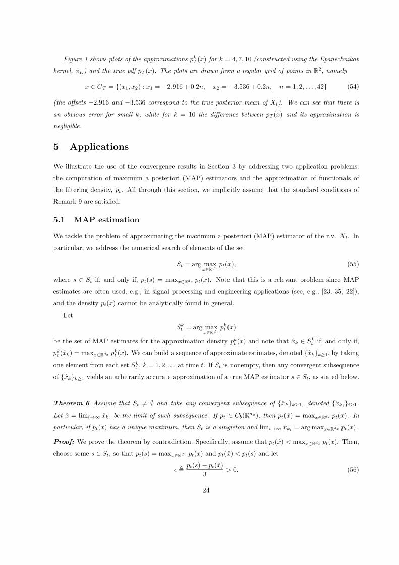
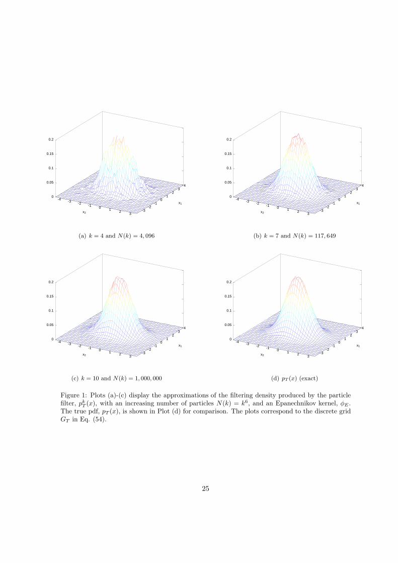
Figure 1 shows plots of the approximations pkT (x) for k = 4, 7, 10 (constructed using the Epanechnikov

kernel, φE) and the true pdf pT (x). The plots are drawn from a regular grid of points in R2, namely

x ∈ GT = (x1, x2) : x1 = −2.916 + 0.2n, x2 = −3.536 + 0.2n, n = 1, 2, . . . , 42 (54)

(the offsets −2.916 and −3.536 correspond to the true posterior mean of Xt). We can see that there is

an obvious error for small k, while for k = 10 the difference between pT (x) and its approximation is

negligible.

5 Applications

We illustrate the use of the convergence results in Section 3 by addressing two application problems:

the computation of maximum a posteriori (MAP) estimators and the approximation of functionals of

the filtering density, pt. All through this section, we implicitly assume that the standard conditions of

Remark 9 are satisfied.

5.1 MAP estimation

We tackle the problem of approximating the maximum a posteriori (MAP) estimator of the r.v. Xt. In

particular, we address the numerical search of elements of the set

St = arg maxx∈Rdx

pt(x), (55)

where s ∈ St if, and only if, pt(s) = maxx∈Rdx pt(x). Note that this is a relevant problem since MAP

estimates are often used, e.g., in signal processing and engineering applications (see, e.g., [23, 35, 22]),

and the density pt(x) cannot be analytically found in general.

Let

Skt = arg max

x∈Rdx

pkt (x)

be the set of MAP estimates for the approximation density pkt (x) and note that xk ∈ Skt if, and only if,

pkt (xk) = maxx∈Rdx pkt (x). We can build a sequence of approximate estimates, denoted xkk≥1, by taking

one element from each set Skt , k = 1, 2, ..., at time t. If St is nonempty, then any convergent subsequence

of xkk≥1 yields an arbitrarily accurate approximation of a true MAP estimator s ∈ St, as stated below.

Theorem 6 Assume that St 6= ∅ and take any convergent subsequence of xkk≥1, denoted xkii≥1.

Let x = limi→∞ xkibe the limit of such subsequence. If pt ∈ Cb(R

dx), then pt(x) = maxx∈Rdx pt(x). In

particular, if pt(x) has a unique maximum, then St is a singleton and limi→∞ xki= argmaxx∈Rdx pt(x).

Proof: We prove the theorem by contradiction. Specifically, assume that pt(x) < maxx∈Rdx pt(x). Then,

choose some s ∈ St, so that pt(s) = maxx∈Rdx pt(x) and pt(x) < pt(s) and let

ǫ ,pt(s)− pt(x)

3> 0. (56)

24

-4-3

-2-1

01

23x2

-3-2

-10

12

34

x1

0

0.05

0.1

0.15

0.2

(a) k = 4 and N(k) = 4, 096

-4-3

-2-1

01

23x2

-3-2

-10

12

34

x1

0

0.05

0.1

0.15

0.2

(b) k = 7 and N(k) = 117, 649

-4-3

-2-1

01

23x2

-3-2

-10

12

34

x1

0

0.05

0.1

0.15

0.2

(c) k = 10 and N(k) = 1, 000, 000

-4-3

-2-1

01

23x2

-3-2

-10

12

34

x1

0

0.05

0.1

0.15

0.2

(d) pT (x) (exact)

Figure 1: Plots (a)-(c) display the approximations of the filtering density produced by the particlefilter, pkT (x), with an increasing number of particles N(k) = k6, and an Epanechnikov kernel, φE .The true pdf, pT (x), is shown in Plot (d) for comparison. The plots correspond to the discrete gridGT in Eq. (54).

25

Now, choose a compact subset K ⊂ Rdx that contain s, xki

i≥1 and x. From Remark 11,

limk→∞ supx∈K |pkt (x) − pt(x)| = 0 a.s., hence there exists m such that for all k ≥ m

supx∈K

∣∣pkt (x) − pt(x)

∣∣ < ǫ. (57)

Moreover, since pt(x) is continuous at every point x ∈ K, we can choose an integer i0 such that for all

i ≥ i0 we obtain

|pt(xki)− pt(x)| < ǫ. (58)

Now, choose an index ℓ such that ℓ ≥ i0 and ℓ ≥ m. Then, for every i, ki > ℓ, we have

pki

t (xki)− pki

t (s) =

<ǫ︷ ︸︸ ︷

pki

t (xki)− pt(xki

)+

<ǫ︷ ︸︸ ︷

pt(xki)− pt(x)

+

=−3ǫ︷ ︸︸ ︷

pt(x)− pt(s)+

<ǫ︷ ︸︸ ︷

pt(s)− pki

t (s) < 0, (59)

where the first term on the right-hand side, pki

t (xki)−pt(xki

) < ǫ, follows from inequality (57), the second

term, pt(xki) − pt(x) < ǫ, follows from inequality (58), the third term, pt(x) − pt(s) = −3ǫ, is due to

the definition in (56) and for the fourth term, pt(s) − pki

t (s) < ǫ, is obtained from the inequality (57).

Therefore, xki/∈ argmaxx∈Rdx pki

t (x) and we arrive at a contradiction. Hence, pt(x) = maxx∈Rdx pt(x).

Remark 12 Note that the whole sequence xk may not converge to a MAP estimate since it may, e.g.,

alternate between different elements of St.

Many global optimization algorithms, such as simulated annealing [5, 26] or accelerated random search

[1], rely only on the evaluation of the objective function and Theorem 6 justifies their use with the

approximation pkt (x). Many other optimization procedures are based on the evaluation of derivates of the

objective function. For example, we may want to use a gradient search method to find a local maximum

of pt(x), i.e., to find a solution of the equation

∇xpt(x) = 0, (60)

where x = (x1, . . . , xdx) and

∇xpt(x) =

∂pt

∂x1

...∂pt

∂xdx

(x) =

Dα1pt...

Dαdx pt

(x),

with αi = (0, . . . ,

i−th︷︸︸︷

1 , . . . , 0). Let x∗ be a solution of (60), i.e., ∇xpt(x∗) = 0. Under the assumptions of

Theorem 1, for every ǫ > 0 there exists kǫ such that, ∀k > kǫ,

−ǫ < Dαipkt (x∗) < ǫ a.s..

26

Therefore,

‖∇xpkt (x

∗)‖ =

√√√√

dx∑

i=1

(

Dαiptk(x∗)

)2

< ǫ√

dx, ∀k < kǫ,

and, since ǫ can be chosen as small as we wish,

limk→∞

‖∇xpkt (x

∗)‖ = 0 a.s.,

which justifies the application of a gradient search procedure using the approximation of the filtering pdf.

Example 2 We illustrate the application of a gradient search procedure using the same example as in

Section 4.4. In particular, we consider the approximation of the maximum of the Gaussian filtering pdf

pT (x), T = 50, using a steepest descent method. Given an approximation pkT (x) of the filtering density

constructed with the Gaussian kernel φG, we run the iterative algorithm

xT (i + 1)k = xT (i)k + a ∇xp

kT (x)

∣∣x=xT (i)k

, i = 0, 1, 2, . . . (61)

with initial condition xT (0)k = (−2,−2)⊤ and step-size parameter a = 0.1. This procedure yields a

sequence of approximations xT (1)k, . . . , xT (i)

k, . . . of the MAP estimator xT . Since for the model of Eq.

(53) it is possible to obtain pT (x) exactly, we have also run a steepest descent search over the true filtering

pdf, namely,

xT (i + 1) = xT (i) + a ∇xpT (x)|x=xT (i) , i = 0, 1, 2, . . . , (62)

that generates the estimates xT (1), . . . , xT (i), . . . for the same initial condition and step size.

The results, using the same sequence of observations as in Section 4.4, are shown in Figure 2.

Specifically, Figures 2(a) and 2(b) show the trajectories described by the estimates xT (1)k, . . . , xT (i)

k, . . .

superimposed over the contour plots of the approximate pdf pkT (x) for k = 5 and k = 9, respectively (and

N(k) = k6). For comparison, Figure 2(c) depicts the sequence xT (1), . . . , xT (i), . . . obtained from the

search over the true density pT (x), together with the corresponding contour plot. We observe that both the

pdf’s and the trajectories described by the search algorithms are very similar.

Figure 3 depicts the sequences of estimates xT (1), . . . , xT (800) and xT (1), . . . , xT (800) computed by the

search algorithms with the approximate and true gradients, ∇pkT (x) and ∇pT (x), respectively, component

wise. We observe that, for k = 9, the approximation is tight in both dimensions.

Similar arguments can be given for other optimization methods based on the derivatives of the density

pt. A relevant example is the Newton method (see, e.g., [3]) as it serves to illustrate the approximation

of second order derivates of pt(x). The Newton iteration for the computation of a solution of Eq. (60)

has the form

xT (i+ 1) = xT (i)− ∆xpT (x)∇xpT (x)|x=xT (i) , (63)

where ∆xpT (x) is the dx × dx Hessian matrix of pT (x).

27

-2

-1

0

1

2

3

-3 -2 -1 0 1 2

x 1

x2

(a) With k = 5 and N(k) = 15, 625.

-2

-1

0

1

2

3

-3 -2 -1 0 1 2

x 1

x2

(b) With k = 9 and N(k) = 531, 441.

-2

-1

0

1

2

3

-3 -2 -1 0 1 2

x 1

x2

(c) With the true posterior pdf, pt.

Figure 2: Trajectories of the gradient search algorithms. Plot (a) shows the estimates produced bythe gradient search algorithm of Eq. (61) superimposed over a contour representation of pk=5

T (x).Plot (b) displays the estimates and contour graph for pk=9

T (x). Plot (c) shows the estimates producedby the gradient search algorithm of Eq. (62) superimposed over a contour representation of pT (x),for comparison.

-2

-1.5

-1

-0.5

0

0.5

0 100 200 300 400 500 600 700 800

x 2

iteration

trueapproximate

-2

-1.5

-1

-0.5

0

0.5

1

1.5

0 100 200 300 400 500 600 700 800

x 1

trueapproximate

Figure 3: Trajectories of the gradient search algorithms (approximate, with k = 9, and exact) onthe horizontal (upper plot) and vertical (lower plot) planes.

28

-2

-1

0

1

2

3

-3 -2 -1 0 1 2

x 1

x2

(a) With k = 7 and N(k) = 117, 649.

-2

-1

0

1

2

3

-3 -2 -1 0 1 2

x 1

x2

(b) With the true posterior pdf, pt.

Figure 4: Trajectories of the Newton algorithms. Plot (a) shows the estimates produced by theNewton search algorithm of Eq. (64) superimposed over a contour representation of pkT (x) for k = 7.Plot (b) shows the estimates produced by the Newton search algorithm of Eq. (63) superimposedover a contour representation of pT (x), for comparison.

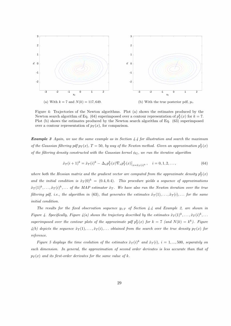
Example 3 Again, we use the same example as in Section 4.4 for illustration and search the maximum

of the Gaussian filtering pdf pT (x), T = 50, by way of the Newton method. Given an approximation pkT (x)

of the filtering density constructed with the Gaussian kernel φG, we run the iterative algorithm

xT (i + 1)k = xT (i)k − ∆xp

kT (x)∇xp

kT (x)

∣∣x=xT (i)k

, i = 0, 1, 2, . . . , (64)

where both the Hessian matrix and the gradient vector are computed from the approximate density pkT (x)

and the initial condition is xT (0)k = (0.4, 0.4). This procedure yields a sequence of approximations

xT (1)k, . . . , xT (i)

k, . . . of the MAP estimator xT . We have also run the Newton iteration over the true

filtering pdf, i.e., the algorithm in (63), that generates the estimates xT (1), . . . , xT (i), . . . for the same

initial condition.

The results for the fixed observation sequence y1:T of Section 4.4 and Example 2, are shown in

Figure 4. Specifically, Figure 4(a) shows the trajectory described by the estimates xT (1)k, . . . , xT (i)

k, . . .

superimposed over the contour plots of the approximate pdf pkT (x) for k = 7 (and N(k) = k6). Figure

4(b) depicts the sequence xT (1), . . . , xT (i), . . . obtained from the search over the true density pT (x) for

reference.

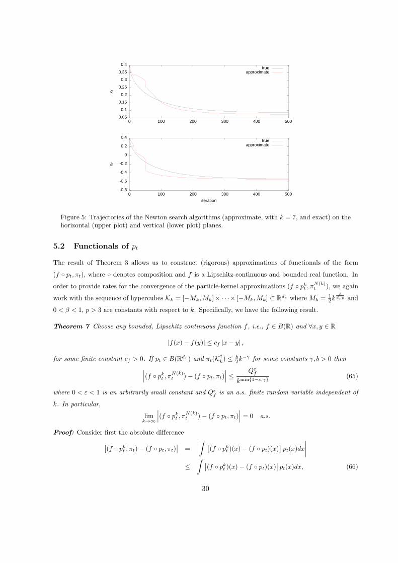
Figure 5 displays the time evolution of the estimates xT (i)k and xT (i), i = 1, ..., 500, separately on

each dimension. In general, the approximation of second order derivates is less accurate than that of

pT (x) and its first-order derivates for the same value of k.

29

-0.8

-0.6

-0.4

-0.2

0

0.2

0.4

0 100 200 300 400 500

x 2

iteration

trueapproximate

0.05

0.1

0.15

0.2

0.25

0.3

0.35

0.4

0 100 200 300 400 500

x 1

trueapproximate

Figure 5: Trajectories of the Newton search algorithms (approximate, with k = 7, and exact) on thehorizontal (upper plot) and vertical (lower plot) planes.

5.2 Functionals of pt

The result of Theorem 3 allows us to construct (rigorous) approximations of functionals of the form

(f pt, πt), where denotes composition and f is a Lipschitz-continuous and bounded real function. In

order to provide rates for the convergence of the particle-kernel approximations (f pkt , πN(k)t ), we again

work with the sequence of hypercubes Kk = [−Mk,Mk]× · · · × [−Mk,Mk] ⊂ Rdx where Mk = 1

2kβ

dxp and

0 < β < 1, p > 3 are constants with respect to k. Specifically, we have the following result.

Theorem 7 Choose any bounded, Lipschitz continuous function f , i.e., f ∈ B(R) and ∀x, y ∈ R

|f(x)− f(y)| ≤ cf |x− y| ,

for some finite constant cf > 0. If pt ∈ B(Rdx) and πt(K†k) ≤ b

2k−γ for some constants γ, b > 0 then

∣∣∣(f pkt , πN(k)

t )− (f pt, πt)∣∣∣ ≤

Qεf

kmin1−ε,γ(65)

where 0 < ε < 1 is an arbitrarily small constant and Qεf is an a.s. finite random variable independent of

k. In particular,

limk→∞

∣∣∣(f pkt , πN(k)

t )− (f pt, πt)∣∣∣ = 0 a.s.

Proof: Consider first the absolute difference

∣∣(f pkt , πt)− (f pt, πt)

∣∣ =

∣∣∣∣

∫[(f pkt )(x)− (f pt)(x)

]pt(x)dx

∣∣∣∣

≤∫∣∣(f pkt )(x) − (f pt)(x)

∣∣ pt(x)dx, (66)

30

where the inequality holds because pt(x) ≥ 0. Using the Lipschitz continuity of f in the integral of Eq.

(66) yields

∣∣(f pkt , πt)− (f pt, πt)

∣∣ ≤ cf

∫∣∣pkt (x)− pt(x)

∣∣ pt(x)dx

≤ cf‖pt‖∞∫∣∣pkt (x) − pt(x)

∣∣ dx, (67)

where the second inequality follows from the assumption pt ∈ B(Rdx) (hence ‖pt‖∞ < ∞). Eq. (67)

together with Theorem 3 readily yields

∣∣(f pkt , πt)− (f pt, πt)

∣∣ ≤ cf‖pt‖∞Qε

kmin1−ε,γ(68)

where 0 < ε < 1 is a constant and Qε is an a.s. finite random variable.

As a second step, consider the difference∣∣∣(f pkt , πN(k)

t )− (f pkt , πt)∣∣∣. Since f ∈ B(R), it follows

that ‖f pkt ‖∞ ≤ ‖f‖∞ independently of k and an application of Proposition 1 yields

E[∣∣∣(f pkt , πN(k)

t )− (f pkt , πt)∣∣∣

q]

≤ cqt‖f‖q∞N(k)

q2

≤ cqt‖f‖q∞kq(2dx+1)

,

where q ≥ 1 and the second inequality holds because N(k) ≥ k2(dx+|1|+1). Using Lemma 1 with

c = cqt‖f‖q∞ and ν = 0 (note that q(2dx + 1) ≥ 2 for any q, dx ≥ 1), we readily obtain the convergence

rate for the absolute error, i.e.,

∣∣∣(f pkt , πN(k)

t )− (f pkt , πt)∣∣∣ ≤ Uε

k1−ε(69)

where 0 < ε < 1 is an arbitrarily small constant and Uε ≥ 0 is an a.s. finite random variable.

To conclude, consider the triangle inequality

∣∣∣(f pkt , πN(k)

t )− (f pt, πt)∣∣∣ ≤

∣∣∣(f pkt , πN(k)

t )− (f pkt , πt)∣∣∣+∣∣(f pkt , πt)− (f pt, πt)

∣∣ . (70)

Substituting (68) and (69) into (70) yields

∣∣∣(f pkt , πN(k)

t )− (f pt, πt)∣∣∣ ≤ Uε

k1−ε+

cf‖pt‖∞Qε

kmin1−ε,γ≤

Qεf

kmin1−ε,γ, (71)

where the random variable Qεf = Uε + cf‖pt‖∞Qε ≥ 0 is a.s. finite and independent of k.

In statistical signal processing and machine learning applications it is often of interest to evaluate

the Shannon entropy of a probability measure π. Assuming that π has a density p w.r.t. the Lebesgue

measure, the entropy of the probability distribution is

H(π) = −(log p, π) = −∫

S

log [p(x)] p(x)dx,

where S is the support of p. In the case of the filtering measure πt, it is natural to think of a particle

approximation of the entropy H(πt) constructed as

H(πt)k = −(log pkt , π

N(k)t ) = − 1

N(k)

N(k)∑

n=1

log pkt (x(n)t ).

31

Unfortunately, the log function is neither bounded nor Lipschitz continuous and, therefore, Theorem 7

does not guarantee the convergence H(πt)k → H(πt). Such a result, however, can be obtained, with a

more specific argument, if we assume the support of the density pt to be compact.

Theorem 8 Let the sequence of observations Y1:T = y1:T (for some large but finite T ) be fixed and assume

that gyt

t ∈ B(Rdx), (gyt

t , ξt) > 0, 1 ≤ t ≤ T , and the integrability conditions in Proposition 1, part (b), are

satisfied. If there exists a compact set S ⊂ Rdx such that

∫

Spt(x)dx = 1 and infx∈S pt(x) > 0, then

limk→∞

∣∣H(πt)

k −H(πt)∣∣ = 0 a.s.

Proof: We apply the triangle inequality to obtain

∣∣∣(− log pkt , π

N(k)t )− (− log pt, πt)

∣∣∣ ≤

∣∣∣(− log pkt , π

N(k)t )− (− log pt, π

N(k)t )

∣∣∣

+∣∣∣(− log pt, π

N(k)t )− (− log pt, πt)

∣∣∣ (72)

and then analyze the two terms in the right-hand side of (72).

The first one can be expanded to yield

∣∣∣(− log pkt , π

N(k)t )− (− log pt, π

N(k)t )

∣∣∣ =

∣∣∣∣∣∣

1

N(k)

N(k)∑

i=1

logpt(x

(i)t )

pkt (x(i)t )

∣∣∣∣∣∣

≤ 1

N(k)

N(k)∑

i=1

∣∣∣∣∣log

pt(x(i)t )

pkt (x(i)t )

∣∣∣∣∣. (73)

The logarithm of a ratio x/y can be upper bounded as

logx

y≤ maxx, y

minx, y − 1, (74)

hence applying (74) into (73) we arrive at

∣∣∣(− log pkt , π

N(k)t )− (− log pt, π

N(k)t )

∣∣∣ ≤ 1

N(k)

N(k)∑

i=1

∣∣∣∣∣∣

max

pkt (x(i)t ), pt(x

(i)t )

min

pkt (x(i)t ), pt(x

(i)t ) − 1

∣∣∣∣∣∣

. (75)

However, from Theorem 2 and Remark 11, limk→∞ pkt (x)/pt(x) = limN→∞ pt(x)/pkt (x) = 1 a.s. for every

x ∈ S. Moreover, since we have assumed infx∈S pt(x) > 0, it follows that for any ǫ > 0 there exists kǫ

independent of x such that, for all k > kǫ,

max

pkt (x(i)t ), pt(x

(i)t )

min

pkt (x(i)t ), pt(x

(i)t ) ≤ 1 + ǫ. (76)

Substituting (76) into (75) yields, for all k > kǫ,

∣∣∣(− log pkt , π

N(k)t )− (− log pt, π

N(k)t )

∣∣∣ ≤ ǫ a.s.

32

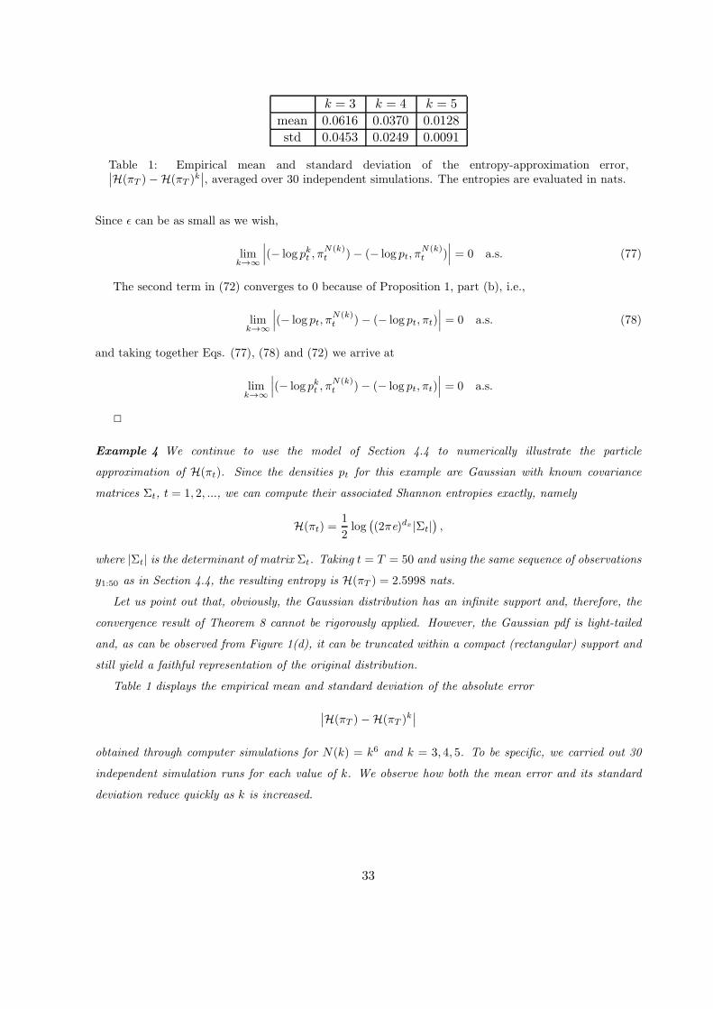
k = 3 k = 4 k = 5

mean 0.0616 0.0370 0.0128

std 0.0453 0.0249 0.0091

Table 1: Empirical mean and standard deviation of the entropy-approximation error,∣∣H(πT )−H(πT )

k∣∣, averaged over 30 independent simulations. The entropies are evaluated in nats.

Since ǫ can be as small as we wish,

limk→∞

∣∣∣(− log pkt , π

N(k)t )− (− log pt, π

N(k)t )

∣∣∣ = 0 a.s. (77)

The second term in (72) converges to 0 because of Proposition 1, part (b), i.e.,

limk→∞

∣∣∣(− log pt, π

N(k)t )− (− log pt, πt)

∣∣∣ = 0 a.s. (78)

and taking together Eqs. (77), (78) and (72) we arrive at

limk→∞

∣∣∣(− log pkt , π

N(k)t )− (− log pt, πt)

∣∣∣ = 0 a.s.

Example 4 We continue to use the model of Section 4.4 to numerically illustrate the particle

approximation of H(πt). Since the densities pt for this example are Gaussian with known covariance

matrices Σt, t = 1, 2, ..., we can compute their associated Shannon entropies exactly, namely

H(πt) =1

2log((2πe)dx |Σt|

),

where |Σt| is the determinant of matrix Σt. Taking t = T = 50 and using the same sequence of observations

y1:50 as in Section 4.4, the resulting entropy is H(πT ) = 2.5998 nats.

Let us point out that, obviously, the Gaussian distribution has an infinite support and, therefore, the

convergence result of Theorem 8 cannot be rigorously applied. However, the Gaussian pdf is light-tailed

and, as can be observed from Figure 1(d), it can be truncated within a compact (rectangular) support and

still yield a faithful representation of the original distribution.

Table 1 displays the empirical mean and standard deviation of the absolute error

∣∣H(πT )−H(πT )

k∣∣

obtained through computer simulations for N(k) = k6 and k = 3, 4, 5. To be specific, we carried out 30

independent simulation runs for each value of k. We observe how both the mean error and its standard

deviation reduce quickly as k is increased.

33

6 Summary

We have addressed the approximation of the sequence of filtering pdf’s of a Markov state-space model

using a particle filter. The numerical technique is conceptually simple. We collect the N particles

generated by the sequential Monte Carlo algorithm and approximate the desired density as the sum of

N scaled kernel functions located at the particle positions. The main contribution of the paper is the

analysis of the convergence of such particle-kernel approximations. In particular, we have first proved

the point-wise convergence of the approximation of the filtering density and its derivatives as the number

of particles is increased and the kernel bandwidth is correspondingly decreased. Explicit convergence

rates are provided and they are sufficient to prove that the approximation errors vanish a.s. Under

mild additional assumptions on the chosen kernel, it is possible to extend the latter result to prove

that the approximation error converges uniformly on the support of the filtering density (rather than

point-wise) and a.s. to 0. We have also found an explicit convergence rate for the supremum of the

approximation error. The analysis establishes a connection between the complexity of the particle filter

and the bandwidth of the kernel function used for estimating the filtering pdf. For a fixed number of

particles N , this relationship yields an optimal value of the bandwidth.

The uniform approximation result has a number of applications. We have first exploited it to prove

the convergence, in total variation distance, of the continuous measure generated by the estimated density

toward the true filtering measure. In a similar vein, we have also shown that the MISE of the sequence

of approximate densities converges (quadratically with the kernel bandwidth) toward 0 when the state

space is compact. For a truncated version of the density approximation, the (random) ISE is also shown

to converge a.s. toward 0 without assuming compactness of the support.

We have also proved that the maxima of the approximate filtering density converge a.s. toward the

true ones. As a consequence, MAP estimation of the state at time t can be carried out using gradient

and Newton search methods on the approximate filtering pdf. We remark that it is sound to apply such

methods on the approximate function, since we have proved convergence also for its derivatives. The last

application we consider is the approximation of functionals of the filtering pdf. We provide a general result

that guarantees the convergence of the particle-kernel approximations for general bounded and Lipschitz

continuous functionals of the filtering density. Finally, we prove that it is also possible to use the proposed

constructs to approximate the Shannon entropy of densities with a compact support. In order to arrive

at this result, we have also proved the convergence of the particle filter approximations of integrals of

unbounded test functions under very mild assumptions (essentially, the integrability of the function up to

fourth order). This is a departure from most existing approaches, which assume bounded test functions.

The theoretical results are complemented with some numerical examples, that include the

approximation of a Gaussian density, its maximization using gradient and Newton methods and the

approximation of its Shannon entropy. The reason to carry out all examples for a Gaussian pdf is that

34

we can compute it exactly using a Kalman filter and, therefore, we can have a proper reference to assess

the performance of the particle-kernel methods. In the case of the Shannon entropy approximation,

the Gaussian distribution does not comply with the compact support assumption. However, being a

light-tailed distribution, our simulations show that accurate estimates can still be computed.

7 Acknowledgements

The work of D. C. was partially supported by the EPSRC Grant number EP/H0005500/1. J. M.

acknowledges the support of the Ministry of Science and Innovation of Spain (program Consolider-Ingenio

2010 CSD2008-00010 COMONSENS and project DEIPRO TEC2009-14504-C02-01).

A Proof of Proposition 1

Part (a) of Proposition 1 is a straightforward consequence of [37, Lemma 1], hence we focus here on part

(b).

We need to introduce an auxiliary result first. Let θii=1,...,N be a collection of zero-mean random

variables, conditionally i.i.d. given a σ-algebra G. In particular, E[θi|G] = 0 for all i and, for any integrable

function h,

E[h(θi)h(θj)|G] = E[h(θi)|G]E[h(θj)|G]

for any i 6= j. We have the following basic inequality

Lemma 2 If the zero-mean, i.i.d. variables θi, i = 1, ..., N , are p-integrable then

E

[(

1

N

N∑

i=1

θi

)p

|G]

≤ c

Np2

E[θp1 |G], (79)

where c is a constant independent of N . In particular, if p > 2,

limN→∞

∣∣∣∣∣

1

N

N∑

i=1

θi

∣∣∣∣∣= 0 a.s. (80)

Proof: The inequality (79) is a straightforward consequence of the Marcinkiewicz-Zygmund inequality

[36] (see also [29, Theorem 3] or [4, Chapter 10]). For p > 2, a standard Borel-Cantelli argument yields

Eq. (80).

Lemma 2 enables us to prove the convergence of particle approximations (f, πNt ) toward (f, πt) when

the function f is integrable w.r.t. πt but not necessarily bounded. We prove this result by induction in t.

For t = 0, the samples x(i)0 , i = 1, ..., N , are i.i.d. with common distribution π0, hence the approximation

πN0 is constructed as πN

0 (dx) = 1N

∑Ni=1 δx(i)

0(dx). It is, therefore, apparent that

E[(f, πN

0 )− (f, π0)]= 0

35

and a simple application of Lemma 2 (with θi = f(x(i)0 )− (f, π0)) yields

limN→∞

∣∣(f, πN

0 )− (f, π0)∣∣ = 0 a.s.

Next, we consider the induction hypothesis

limN→∞

∣∣(f, πN

t )− (f, πt)∣∣ = 0 a.s. (81)

and study the particle approximations at time t+ 1.

We start with the convergence of integrals of the form (f, ξt+1), where ξt+1 = τt+1πt, as defined in

Eq. (7). The particle approximation of ξt has the form

ξNt (dx) =1

N

N∑

n=1

δx(n)t

(dx),

hence the integral (f, ξNt+1) has conditional mean

E[(f, ξNt+1)|Ft] = (f, τt+1πNt ),

given the σ-algebra Ft = σ(

x(n)l , x

(n)s : 1 ≤ n ≤ N, 0 ≤ l ≤ t, 0 < s ≤ t

)

. In particular, the random

variables θi = f(x(i)t+1)− (f, τt+1π

Nt ) are centered and i.i.d., and Lemma 2 yields

E[∣∣(f, ξNt+1)− (f, τt+1π

Nt )∣∣p |Ft

]

= E

[∣∣∣∣∣

1

N

N∑

i=1

θi

∣∣∣∣∣

p

|Ft

]

≤˜ctE[θp1 |Ft]

Np2

, (82)

where ˜ct is a constant w.r.t. N . Since both f and ft+1 are p-integrable, it follows that E[θp1 |Ft] is a finite

and non-negative random variable. Taking unconditional expectations on both sides of (82), we arrive at

E[∣∣(f, ξNt+1)− (f, τt+1π

Nt

∣∣p]

≤ ct

Np2

, (83)

where ct = ˜ctE [E[θp1 |Ft]] is a constant w.r.t. N . From (83) it is straightforward to prove (e.g., using

Lemma 1 or a Borel-Cantelli argument with p > 2) that

limN→∞

∣∣(f, ξNt+1)− (f, τt+1π

Nt )∣∣ = 0 a.s. (84)

Moreover, given the function ft+1(x) =∫f(x′)τt+1(dx

′|x), we can write (f, τt+1πNt ) = (ft+1, π

Nt ) and

(f, τt+1, πt) = (ft+1, πt) and, as a consequence,

∣∣(f, τt+1π

Nt )− (f, τt+1πt)

∣∣ =

∣∣(ft+1, π

Nt )− (ft+1, πt)

∣∣ .

Note that ft+1 is a real function on Rdx and we have assumed that (fp

t+1, πt) < ∞. Therefore, for p > 2,

we can apply the induction hypothesis (81) to arrive at

limN→∞

∣∣(ft+1, π

Nt )− (ft+1, πt)

∣∣ = 0 a.s. (85)

36

It is now straightforward to prove the convergence of (f, ξNt+1). Specifically, from the triangle inequality

we obtain

limN→∞

∣∣(f, ξNt+1)− (f, ξt+1)

∣∣ ≤ lim

N→∞

∣∣(f, ξNt+1)− (f, τt+1π

Nt )∣∣ + lim

N→∞

∣∣(f, τt+1π

Nt )− (f, ξt+1)

∣∣ (86)

and, since ξt+1 = τt+1πt, substituting (84) and (85) into (86) yields

limN→∞

∣∣(f, ξNt+1)− (f, ξt+1)

∣∣ = 0 a.s. (87)

In order to analyze the approximations (f, πNt+1), we first consider the measure

πNt+1(dx) =

N∑

n=1

w(n)t+1δx(n)

t+1

(dx), where w(n)t+1 =

gyt+1

t+1 (x(n)t+1)

∑Nk=1 g

yt+1

t+1 (x(n)t+1)

obtained immediately after the computation of the weights in the particle filter. Integrals w.r.t. πNt+1 can

be written in terms of gyt+1

t+1 and ξNt+1, namely

(f, πNt+1) =

(fgyt+1

t+1 , ξNt+1)

(gyt+1

t+1 , ξNt+1).

This is natural, though, since from the Bayes theorem we readily derive the same relationship between

πt+1 and ξt+1,

(f, πt+1) =(fg

yt+1

t+1 , ξt+1)

(gyt+1

t+1 , ξt+1),

and the difference (f, πNt+1)− (f, πt+1) can, therefore, be written as

(f, πNt+1)− (f, πt+1) =

(fgyt+1

t+1 , ξNt+1)

(gyt+1

t+1 , ξNt+1)− (fg

yt+1

t+1 , ξt+1)

(gyt+1

t+1 , ξt+1)± (fg

yt+1

t+1 , ξNt+1)

(gyt+1

t+1 , ξt+1)

=(fg

yt+1

t+1 , ξNt+1)− (fgyt+1

t+1 , ξt+1)

(gyt+1

t+1 , ξt+1)

+(fg

yt+1

t+1 , ξNt+1)

(gyt+1

t+1 , ξNt+1)× (g

yt+1

t+1 , ξt+1)− (gt+1, ξNt+1)

(gyt+1

t+1 , ξt+1). (88)

Note that, since gyt+1

t+q ∈ B(Rdx), Eq. (87) yields

limN→∞

∣∣(g

yt+1

t+1 , ξt+1)− (gt+1, ξNt+1)

∣∣ = 0 a.s. (89)

and, since the assumptions in the Lemma impose that

(gyt+1

t+1 , ξt+1) > 0, (90)

it follows that

limN→∞

(gt+1, ξNt+1) > 0 a.s. (91)

Also as a consequence of gyt+1

t+1 ∈ B(Rdx), the function fgyt+1

t+1 is p-integrable and Eq. (87) guarantees, for

p > 2, that

limN→∞

∣∣(fg

yt+1

t+1 , ξt+1)− (fgt+1, ξNt+1)

∣∣ = 0 a.s. (92)

37

and, in particular

limN→∞

(fgt+1, ξNt+1) < ∞ a.s. (93)

Taking Eqs. (90) and (91) together, we deduce that the denominator of (88) is a.s. positive (as N → ∞).

Similarly, Eqs. (89), (92) and (93) show that the numerator of (88) converges to 0 a.s. as N → ∞.

Therefore,

limN→∞

∣∣(f, πN

t+1)− (f, πt+1)∣∣ = 0 a.s. (94)

On the other hand, the difference |(f, πNt+1) − (f, πt+1)| also converges to 0 a.s. Indeed, given the

σ-algebra Ft = σ(

x(n)r , x

(n)s ; n = 1, . . . , N, 0 ≤ r < t, 0 < s ≤ t

)

,

E[

f(x(i)t+1)|Ft+1

]

= (f, πNt+1), i = 1, . . . , N,

hence the random variables θi = f(x(i)t+1)− (f, πN

t+1) are centered and conditionally i.i.d. given Ft+1. As

a consequence, Lemma 2 yields

E

[∣∣∣∣∣

1

N

N∑

i=1

θi

∣∣∣∣∣

p

|Ft+1

]

≤˜ct+1E[θp1 |Ft+1]

Np2

, (95)

where ˜ct+1 is a constant and 1N

∑Ni=1 θi = (f, πN

t+1)− (f, πNt+1). If we take full expectations on both sides

of (95), we obtain

E[∣∣(f, πN

t+1)− (f, πNt+1)

∣∣p |Ft+1

]

≤ ct+1

Np2

, (96)

where ct+1 = ˜ct+1E[E[θp1 |Ft+1]

]is a finite constant. For p > 2, from Eq. (96), we readily deduce that

limN→∞

∣∣(f, πN

t+1)− (f, πNt+1)

∣∣ = 0 a.s., (97)

using either Lemma 1 or a standard Borel-Cantelli argument.

Finally, taking together (94), (97) and the triangle inequality

∣∣(f, πN

t+1)− (f, πt+1)∣∣ ≤

∣∣(f, πN

t+1)− (f, πNt+1)

∣∣+∣∣(f, πN

t+1)− (f, πt+1)∣∣ ,

we arrive at limN→∞

∣∣(f, πN

t+1)− (f, πt+1)∣∣ = 0 a.s.

B Proof of Lemma 1

Choose a constant β such that ν < β < p− 1 and define the random variable

Uβ,p =

∞∑

m=1

mp−1−β(θm)p.

The variable Uβ,p is obviously non-negative and, additionally, it has a finite mean, E[Uβ,p] < ∞. Indeed,

from Fatou’s lemma

E[Uβ,p

]≤

∞∑

m=1

mp−1−βE[(θm)p] ≤ c

∞∑

m=1

m−1−β+ν ,

38

where the second inequality follows from Eq. (20). Since β−ν > 0, it follows that∑∞

m=1 m−1−(β−ν) < ∞,

hence E[Uβ,p] < ∞.

We use the so-defined random variable Uβ,p in order to determine the convergence rate of θk.

Obviously, kp−1−β(θk)p ≤ Uβ,p and solving for θk yields

θk ≤(Uβ,p

) 1p

k1−1+βp

.

If we define ε = 1+βp and Uε =

(Uβ,p

) 1p , the we obtain the inequality

θk ≤ Uε

k1−ε.

Since E[Uβ,p] < ∞, it follows that E [(Uε)p)] < ∞, hence Uε is a.s. finite. Also, we recall that

ν < β < p− 1, therefore 1+νp < ε < 1.

References

[1] M. J. Appel, R. Labarre, and D. Radulovic. On accelerated random search. SIAM Journal on

Optimization, 14(3):708–730, 2003.

[2] A. Bain and D. Crisan. Fundamentals of Stochastic Filtering. Springer, 2008.

[3] J. F. Bonnans and C. Lemarechal. Numerical optimization: theoretical and practical aspects. Springer-

Verlag New York Inc, 2006.

[4] Y. S. Chow and H. Teicher. Probability theory independence, interchangeability, martingales (third

edition). Springer, 2003.

[5] A. Corana, M. Marchesi, C. Martini, and S. Ridella. Minimizing multimodal functions of continuous

variables with the “simulated annealing” algorithm. ACM Transactions on Mathematical Software,

13(3):262–280, September 1987.

[6] T. M. Cover and J. A. Thomas. Elements of Information Theory. Wiley-Interscience, New York

(USA), 1991.

[7] D. Crisan. Particle filters - a theoretical perspective. In A. Doucet, N. de Freitas, and N. Gordon,

editors, Sequential Monte Carlo Methods in Practice, chapter 2, pages 17–42. Springer, 2001.

[8] D. Crisan, P. Del Moral, and T.J. Lyons. Non-linear filtering using branching and interacting particle

systems. Markov Processes Related Fields, 5(3):293–319, 1999.

[9] D. Crisan and A. Doucet. Convergence of sequential Monte Carlo methods. Technical Report

Cambridge University (CUED/FINFENG/TR381), 2000.

[10] D. Crisan and A. Doucet. A survey of convergence results on particle filtering. IEEE Transactions

Signal Processing, 50(3):736–746, March 2002.

39

[11] T. A. Dean, S. S. Singh, A. Jasra, and G. W. Peters. Parameter estimation for hidden Markov models

with intractable likelihoods. arXiv, 1103.5399v1[math.ST], 2011.

[12] P. Del Moral. Non-linear filtering: interacting particle solution. Markov Processes and Related Fields,

2:555–580, 1996.

[13] P. Del Moral. Non-linear filtering using random particles. Theory of Probability and its Applications,

40(4):690–701, 1996.

[14] P. Del Moral. Feynman-Kac Formulae: Genealogical and Interacting Particle Systems with

Applications. Springer, 2004.

[15] P. Del Moral, A. Doucet, and S. Singh. Uniform stability of a particle approximation of the optimal

filter derivative. arXiv, 1106.2525v1[math.ST], 2011.

[16] P. Del Moral and L. Miclo. Branching and interacting particle systems. Approximations of Feynman-

Kac formulae with applications to non-linear filtering. Lecture Notes in Mathematics, pages 1–145,

2000.

[17] L. Devroye and L. Gyorfi. Nonparametric Density Estimation: The L1 View. Wiley, 1985.

[18] R. Douc, O. Cappe, and E. Moulines. Comparison of resampling schemes for particle filtering. In

Proceedings of the 4th International Symposium on Image and Signal Processing and Analysis, pages

64–69, September 2005.

[19] A. Doucet, N. de Freitas, and N. Gordon. An introduction to sequential Monte Carlo methods.

In A. Doucet, N. de Freitas, and N. Gordon, editors, Sequential Monte Carlo Methods in Practice,

chapter 1, pages 4–14. Springer, 2001.

[20] A. Doucet, N. de Freitas, and N. Gordon, editors. Sequential Monte Carlo Methods in Practice.

Springer, New York (USA), 2001.

[21] A. Doucet, S. Godsill, and C. Andrieu. On sequential Monte Carlo Sampling methods for Bayesian

filtering. Statistics and Computing, 10(3):197–208, 2000.

[22] L. Frenkel and M. Feder. Recursive expectation-maximization (EM) algorithms for time-varying

parameters with applications to multiple target tracking. IEEE Transactions Signal Processing,

47(2):306–320, February 1999.

[23] J. L. Gauvain and C. H. Lee. Bayesian learning for hidden Markov model with Gaussian mixture

state observation densities. Speech Communication, 11(2-3):205–213, 1992.

[24] S. Godsill, A. Doucet, and M. West. Maximum a posteriori sequence estimation using Monte Carlo

particle filters. Annals of the Institute of Statistical Mathematics, 53(1):82–96, March 2001.

[25] N. Gordon, D. Salmond, and A. F. M. Smith. Novel approach to nonlinear and non-Gaussian Bayesian

state estimation. IEE Proceedings-F, 140(2):107–113, 1993.

40

[26] A.-R. Hedar and M. Fukushima. Derivative-free filter simulated annealing method for constrained

continuous global optimization. Journal of Global Optimization, 35:521–549, 2006.

[27] K. Heine and D. Crisan. Uniform approximations of discrete-time filters. Advances in Applied

Probability, 40(4):979–1001, 2008.

[28] X.L. Hu, T.B. Schon, and L. Ljung. A basic convergence result for particle filtering. IEEE

Transactions on Signal Processing, 56(4):1337–1348, 2008.

[29] R. Ibragimov and Sh. Sharakhmetov. Analogues of Khintchine, Marcinkiewicz-Zygmund and

Rosenthal inequalities for symmetric statistics. Scandinavian Journal of Statistics, 26(4):pp. 621–633,

1999.

[30] R. E. Kalman. A new approach to linear filtering and prediction problems. Journal of Basic

Engineering, 82:35–45, 1960.

[31] G. Kitagawa. Monte Carlo filter and smoother for non-Gaussian nonlinear state-space models. J.

Comput. Graph. Statist., 1:1–25, 1996.

[32] H. R. Kunsch. Recursive Monte Carlo filters: Algorithms and theoretical bounds. The Annals of

Statistics, 33(5):1983–2021, 2005.

[33] F. LeGland and N. Oudjane. Stability and uniform approximation of nonlinear filters using the

Hilbert metric and application to particle filters. Annals of Applied Probability, pages 144–187, 2004.

[34] J. S. Liu and R. Chen. Sequential Monte Carlo methods for dynamic systems. Journal of the

American Statistical Association, 93(443):1032–1044, September 1998.

[35] A. Logothetis and V. Krishnamurthy. Expectation maximization algorithms for map estimation of

jump markov linear systems. IEEE Transactions on Signal Processing, 47(8):2139–2156, 1999.

[36] J. Marcinkiewicz and A. Zygmund. Quelques theoremes sur les fonctions independantes’). Fund.

Math, 29:60–90, 1937.

[37] J. Mıguez, D. Crisan, and P. M. Djuric. On the convergence of two sequential Monte Carlo methods

for maximum a posteriori sequence estimation and stochastic global optimization. Statistics and

Computing, DOI: 10.1007/s11222-011-9294-4, 2011.

[38] C. Musso, N. Oudjane, and F. LeGland. Improving regularised particle filters. In A. Doucet,

N. de Freitas, and N. Gordon, editors, Sequential Monte Carlo Methods in Practice, chapter 12,

pages 247–272. Springer, 2001.

[39] K. Najim, E. Ikonen, and P. Del Moral. Open-loop regulation and tracking control based on a

genealogical decision tree. Neural Computing and Applications, 15:339–349, 2006.

[40] B. W. Silverman. Density Estimation for Statistics and Data Analysis. Chapman & Hall/CRC, Boca

Raton (FL, USA), 1986.

41

[41] J. S. Simonoff. Smoothing Methods in Statistics. Springer-Verlag, New York, 1996.

[42] M. P. Wand and M. C. Jones. Kernel Smoothing. Chapman-Hall/CRC, 1995.

42