PARTIALLY SUPERVISED CLASSIFICATION OF TEXT DOCUMENTS

PARTIALLY SUPERVISED CLASSIFICATION

OF TEXT DOCUMENTS

authors:

B. Liu, W.S. Lee, P.S. Yu, X. Li

presented by Rafal Ladysz

2

WHAT IT IS ABOUT• the paper shows:

– document classification– one class of positively labeled documents– accompanied by a set of unlabeled, mixed documents– the above enables to build accurate classifiers– using EM algorithm based on NB classification– strengthening the EM by so called “spy documents”– experimental results for illustration

• we will browse through the paper and– emphasize/refresh some of its theoretical aspects– try to understand the methods described– look at results obtained and interpret them

3

AGENDA (informally)• problem described• document classification• PSC - general assumptions• PSC - some theory• Bayes basics• EM in general• I- EM algorithm• introducing spies• I-S-EM algorithm• selecting classifier• experimental data• results and conclusions• references

4

KEY PROBLEM – a big picture

• no labeled negative training data (text documents)• only a (small) set of relevant (positive) documents• necessity to classify unlabeled text documents• importance:

– finding relevant text on the web – or digital libraries

5

DOCUMENT CLASSIFICATION – some

techniques used

• kNN (Nearest Neighbors)

• Linear Least Squares Fit

• SVM

• Naive Bayes: utilized here

6

PARTIALLY SUPERVISED CLASSIFICATION (PSC) – theoretical foundations

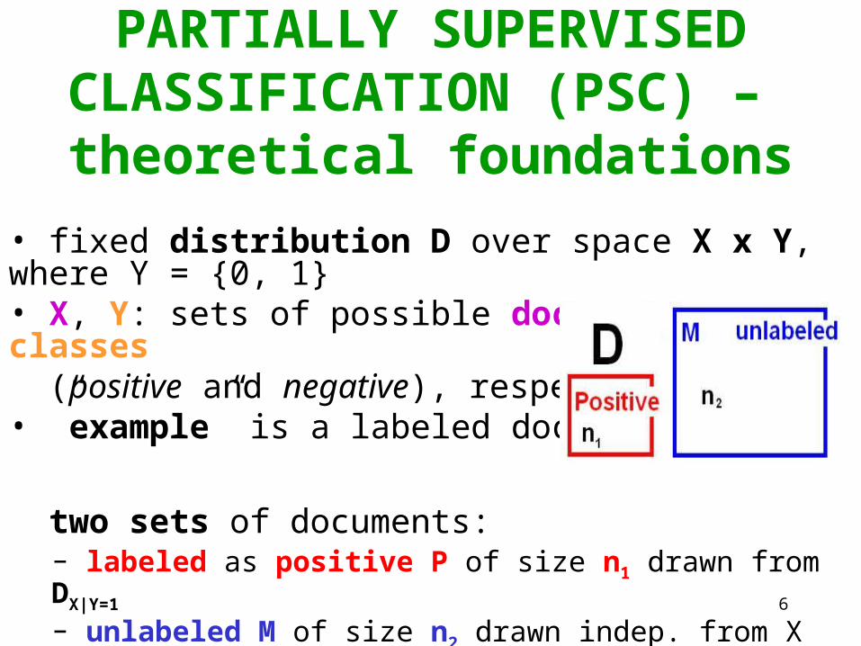
• fixed distribution D over space X x Y, where Y = {0, 1}• X, Y: sets of possible documents, classes (positive and negative), respectively• ”example” is a labeled document

two sets of documents:– labeled as positive P of size n1 drawn from DX|Y=1

– unlabeled M of size n2 drawn indep. from X for DX

remark: there might be some relevant documents in M (but we don’t know about their existence!)

7

PSC cont.

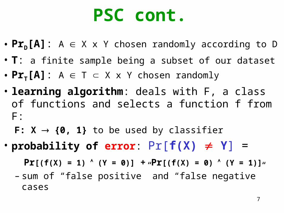
• PrD[A]: A X x Y chosen randomly according to D

• T: a finite sample being a subset of our dataset

• PrT[A]: A T X x Y chosen randomly

• learning algorithm: deals with F, a class of functions and selects a function f from F:F: X {0, 1} to be used by classifier

• probability of error: Pr[f(X) Y] = Pr[(f(X) = 1) (Y = 0)] + Pr[(f(X) = 0) (Y = 1)]

– sum of “false positive” and “false negative” cases

8

PSC: approximations (1)

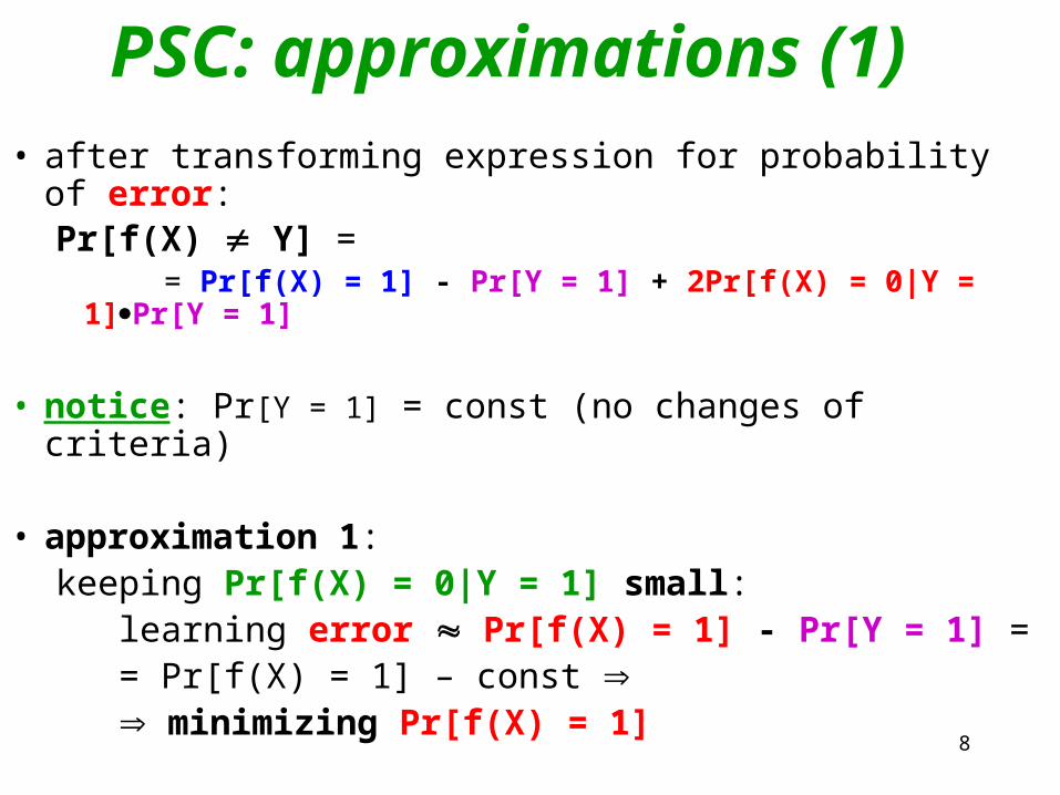
• after transforming expression for probability of error: Pr[f(X) Y] = = Pr[f(X) = 1] - Pr[Y = 1] + 2Pr[f(X) = 0|Y = 1]Pr[Y = 1]

• notice: Pr[Y = 1] = const (no changes of criteria)

• approximation 1: keeping Pr[f(X) = 0|Y = 1] small: learning error Pr[f(X) = 1] - Pr[Y = 1] = = Pr[f(X) = 1] – const minimizing Pr[f(X) = 1]

9

PSC: approximations (2)

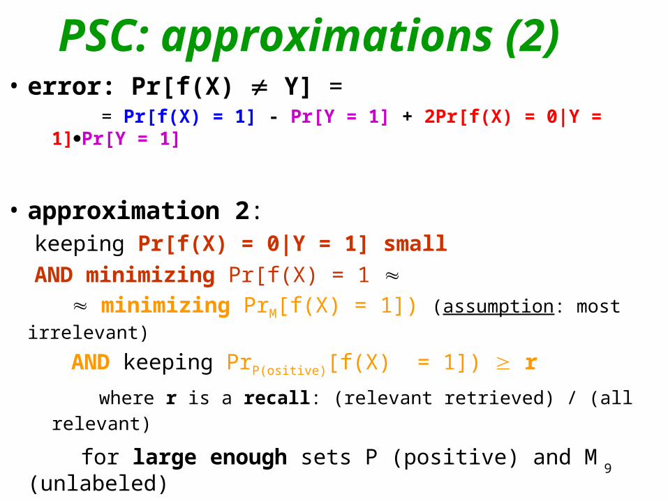
• error: Pr[f(X) Y] = = Pr[f(X) = 1] - Pr[Y = 1] + 2Pr[f(X) = 0|Y = 1]Pr[Y = 1]

• approximation 2:keeping Pr[f(X) = 0|Y = 1] small

AND minimizing Pr[f(X) = 1 minimizing PrM[f(X) = 1]) (assumption: most irrelevant)

AND keeping PrP(ositive)[f(X) = 1]) r

where r is a recall: (relevant retrieved) / (all relevant)

for large enough sets P (positive) and M (unlabeled)

10

CONSTRAINT OPTIMIZATION

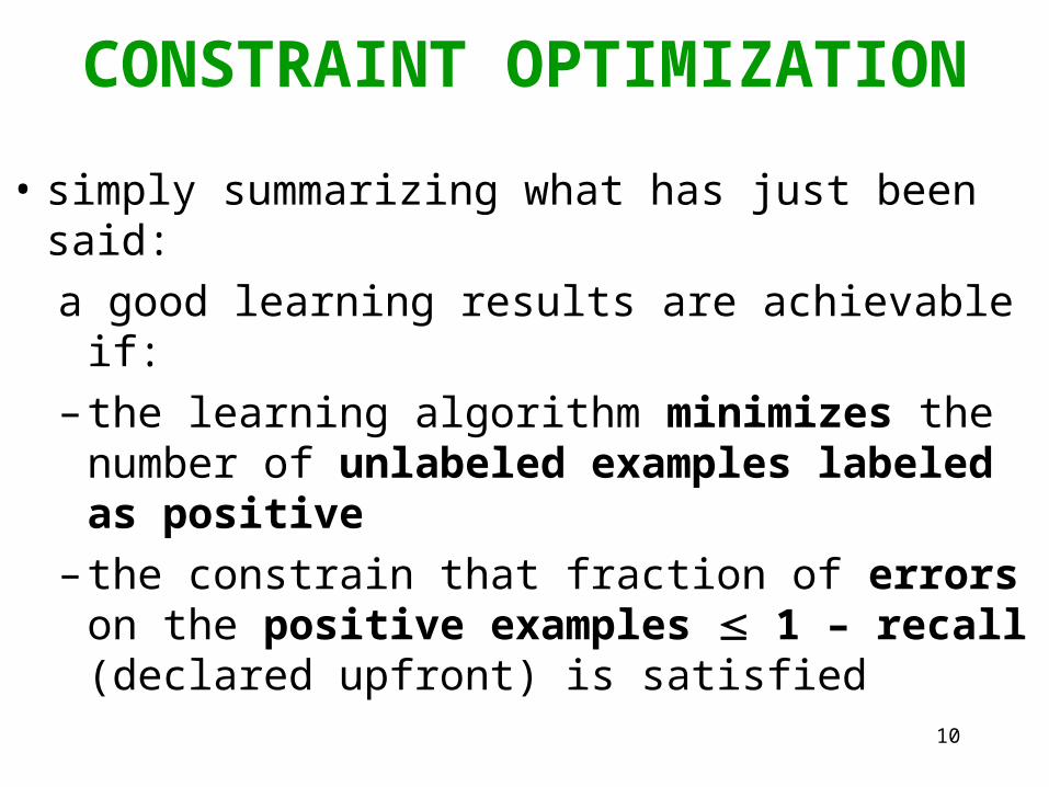
• simply summarizing what has just been said:

a good learning results are achievable if:

– the learning algorithm minimizes the number of unlabeled examples labeled as positive

– the constrain that fraction of errors on the positive examples 1 – recall (declared upfront) is satisfied

11

COMPLEXITY FUNCTION (CF)

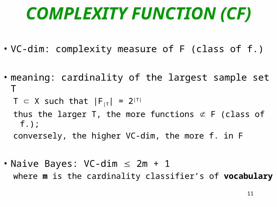
• VC-dim: complexity measure of F (class of f.)

• meaning: cardinality of the largest sample set TT X such that |F|T| = 2|T|

thus the larger T, the more functions F (class of f.);

conversely, the higher VC-dim, the more f. in F

• Naive Bayes: VC-dim 2m + 1 where m is the cardinality classifier’s of vocabulary

12

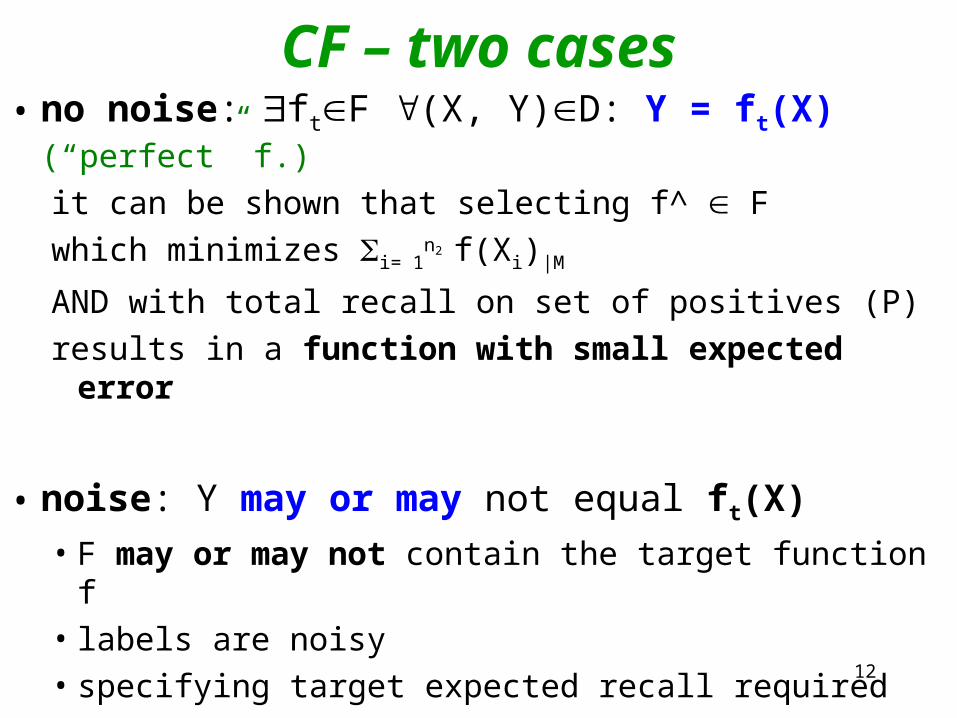
CF – two cases• no noise: ftF (X, Y)D: Y = ft(X) (“perfect” f.)

it can be shown that selecting f^ F

which minimizes i= 1n2 f(Xi)|M

AND with total recall on set of positives (P)

results in a function with small expected error

• noise: Y may or may not equal ft(X)

• F may or may not contain the target function f• labels are noisy• specifying target expected recall required

13

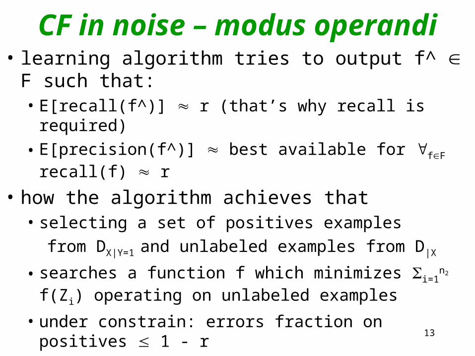
CF in noise – modus operandi

• learning algorithm tries to output f^ F such that:• E[recall(f^)] r (that’s why recall is required)

• E[precision(f^)] best available for fF recall(f) r

• how the algorithm achieves that• selecting a set of positives examples

from DX|Y=1 and unlabeled examples from D|X

• searches a function f which minimizes i=1n2 f(Zi)

operating on unlabeled examples• under constrain: errors fraction on positives 1 - r

14

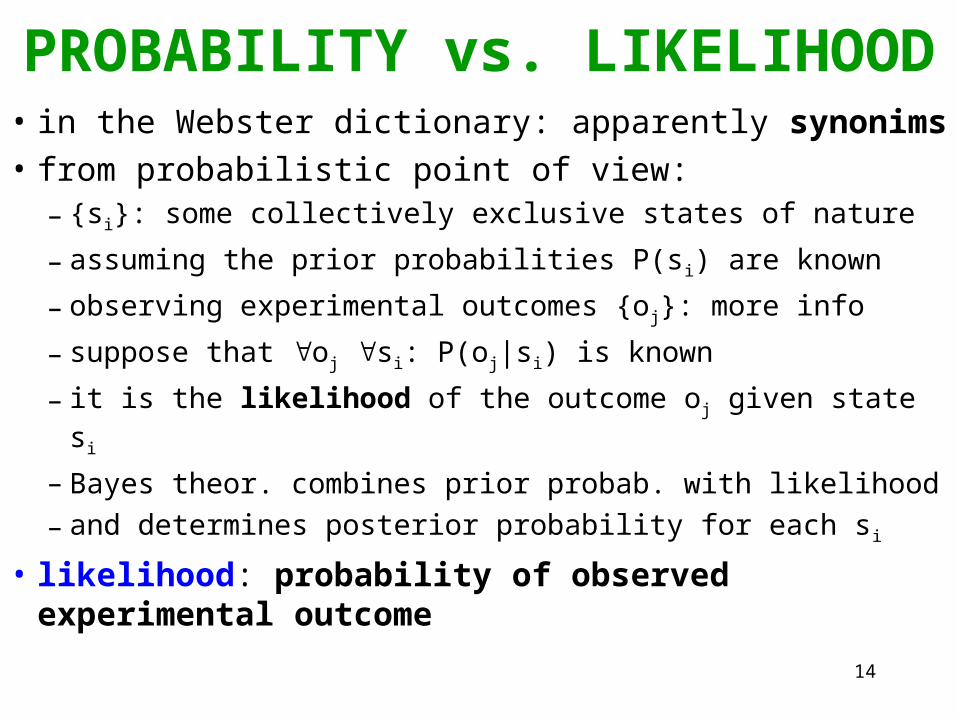
PROBABILITY vs. LIKELIHOOD

• in the Webster dictionary: apparently synonims• from probabilistic point of view:

– {si}: some collectively exclusive states of nature

– assuming the prior probabilities P(si) are known

– observing experimental outcomes {oj}: more info

– suppose that oj si: P(oj|si) is known

– it is the likelihood of the outcome oj given state si

– Bayes theor. combines prior probab. with likelihood

– and determines posterior probability for each si

• likelihood: probability of observed experimental outcome

15

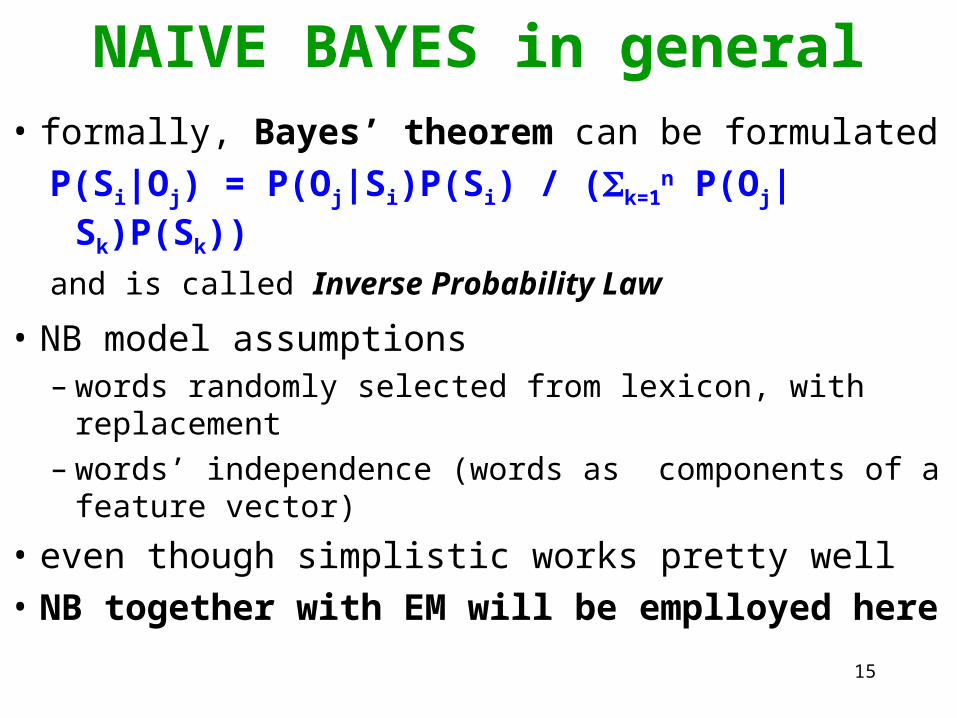
NAIVE BAYES in general• formally, Bayes’ theorem can be formulated

P(Si|Oj) = P(Oj|Si)P(Si) / (k=1n P(Oj|Sk)P(Sk))

and is called Inverse Probability Law

• NB model assumptions – words randomly selected from lexicon, with

replacement– words’ independence (words as components of a

feature vector)

• even though simplistic works pretty well

• NB together with EM will be emplloyed here

16

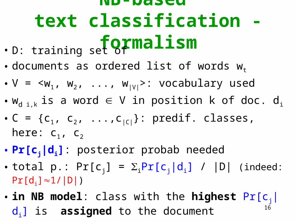
NB-based text classification -

formalism• D: training set of

• documents as ordered list of words wt

• V = <w1, w2, ..., w|V|>: vocabulary used

• wd i,k is a word V in position k of doc. di

• C = {c1, c2, ...,c|C|}: predif. classes, here: c1, c2

• Pr[cj|di]: posterior probab needed

• total p.: Pr[cj] = iPr[cj|di] / |D| (indeed: Pr[di]1/|D|)

• in NB model: class with the highest Pr[cj|di] is assigned to the document

17

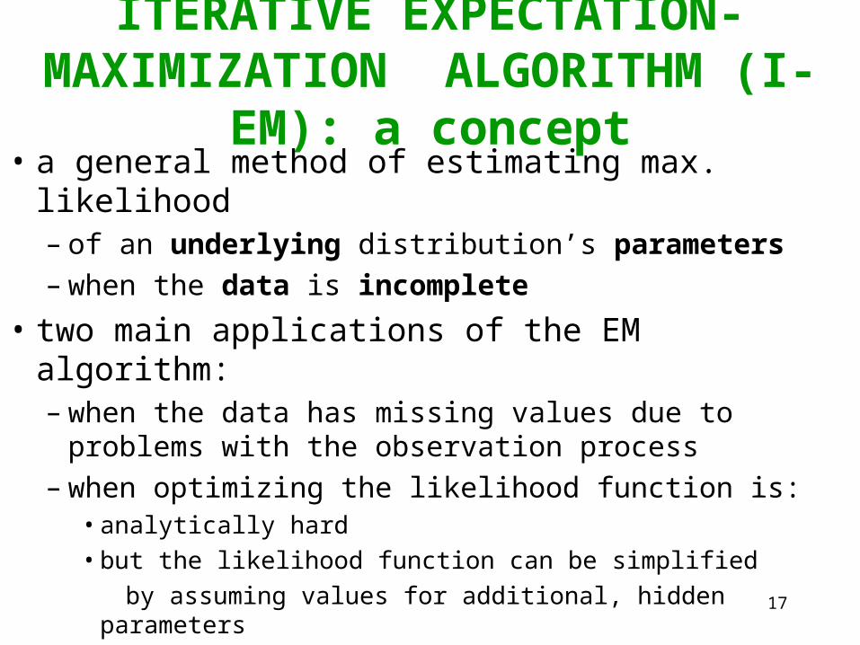
ITERATIVE EXPECTATION-MAXIMIZATION ALGORITHM (I-

EM): a concept• a general method of estimating max. likelihood

– of an underlying distribution’s parameters– when the data is incomplete

• two main applications of the EM algorithm:– when the data has missing values due to problems

with the observation process

– when optimizing the likelihood function is: • analytically hard • but the likelihood function can be simplified

by assuming values for additional, hidden parameters

18

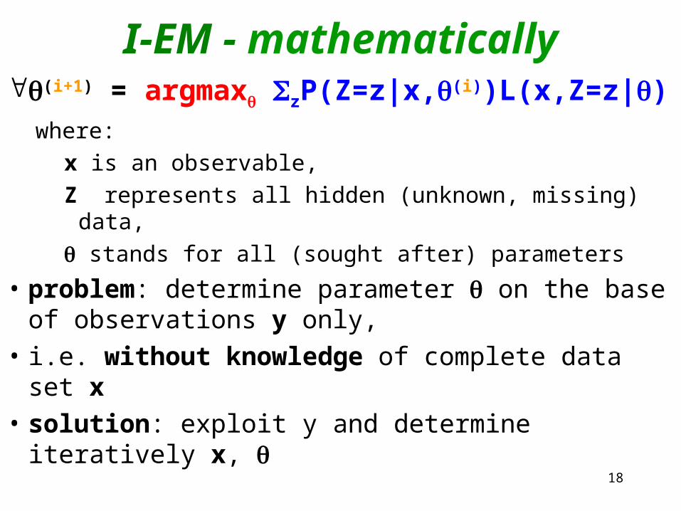
I-EM - mathematically(i+1) = argmax zP(Z=z|x,(i))L(x,Z=z|)

where:

x is an observable,

Z represents all hidden (unknown, missing) data,

stands for all (sought after) parameters

• problem: determine parameter on the base of observations y only,

• i.e. without knowledge of complete data set x

• solution: exploit y and determine iteratively x,

19

20

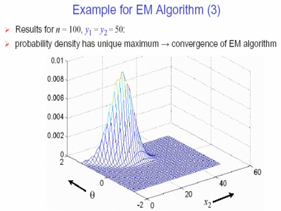
21

22

I-EM properties• simple but computationally demanding

• convergence behavior– no guarantee for global optimum– initial point (0) determines if global optimum is

reachable (or algorithm gets stuck in local optimum)– stable: likelihood function increases in every

iteration until (local if not global) optimum reached

• M(aximum) L(ikelihood) are fixed points in EM

23

I-EM ALGORITHM – why and how

• for the classification (main objective)posterior probability Pr[cj|di] needed

• probabilities will converge during iterations

• EM: iterative algorithm for max. likelihood estimation for incomplete data (interpolates)

• two steps:1. expectation: filling in missing data

2. maximization: parameters estimating

next iteration launched

24

I-EM: symbols used• symbols used:

D: training set of documents each documant: ordered list of words wdi,k: kth word in ith document

each wdi,k V = {w1, w2, ..., w|V|} (vocabulary)

vocabulary: all words to be classified C = {c1, c2}: predefine dclasses (only 2)

25

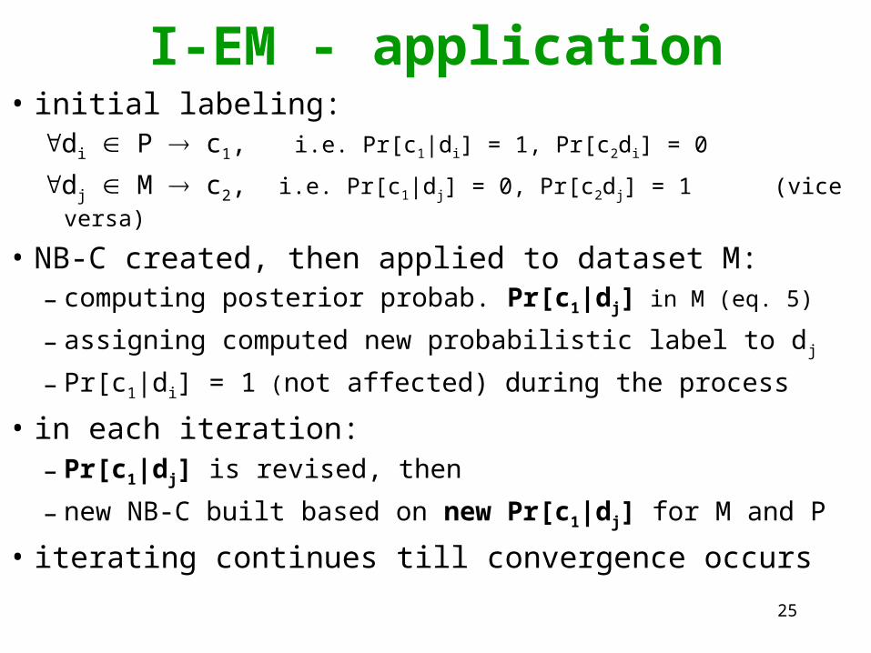
I-EM - application• initial labeling:

di P c1, i.e. Pr[c1|di] = 1, Pr[c2di] = 0

dj M c2, i.e. Pr[c1|dj] = 0, Pr[c2dj] = 1 (vice versa)

• NB-C created, then applied to dataset M:– computing posterior probab. Pr[c1|dj] in M (eq. 5)

– assigning computed new probabilistic label to dj

– Pr[c1|di] = 1 (not affected) during the process

• in each iteration:– Pr[c1|dj] is revised, then

– new NB-C built based on new Pr[c1|dj] for M and P

• iterating continues till convergence occurs

26

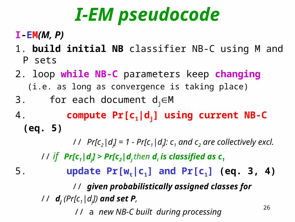
I-EM pseudocodeI-EM(M, P)

1. build initial NB classifier NB-C using M and P sets

2. loop while NB-C parameters keep changing(i.e. as long as convergence is taking place)

3. for each document djM

4. compute Pr[c1|dj] using current NB-C (eq. 5)

// Pr[c2|dj] = 1 - Pr[c1|dj]: c1 and c2 are collectively excl.

// if Pr[c1|dj] > Pr[c2|dj then di is classified as c1

5. update Pr[wt|c1] and Pr[c1] (eq. 3, 4)

// given probabilistically assigned classes for

// dj (Pr[c1|dj]) and set P,

// a new NB-C built during processing

27

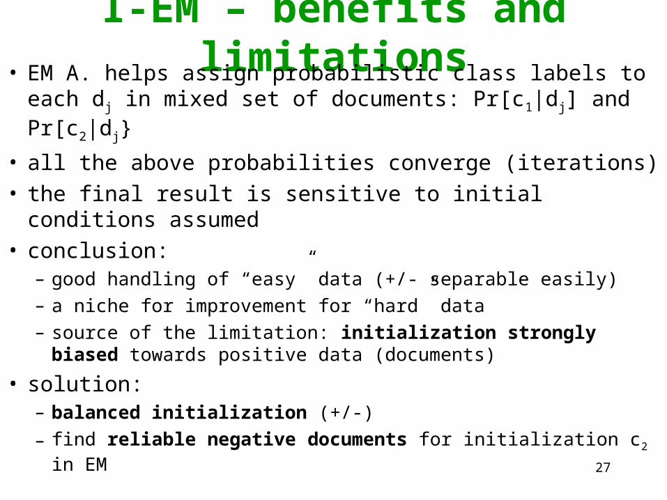
I-EM – benefits and limitations• EM A. helps assign probabilistic class labels to each d j

in mixed set of documents: Pr[c1|dj] and Pr[c2|dj}

• all the above probabilities converge (iterations)• the final result is sensitive to initial conditions assumed• conclusion:

– good handling of “easy” data (+/- separable easily)– a niche for improvement for “hard” data– source of the limitation: initialization strongly biased

towards positive data (documents)

• solution: – balanced initialization (+/-)

– find reliable negative documents for initialization c2 in EM

28

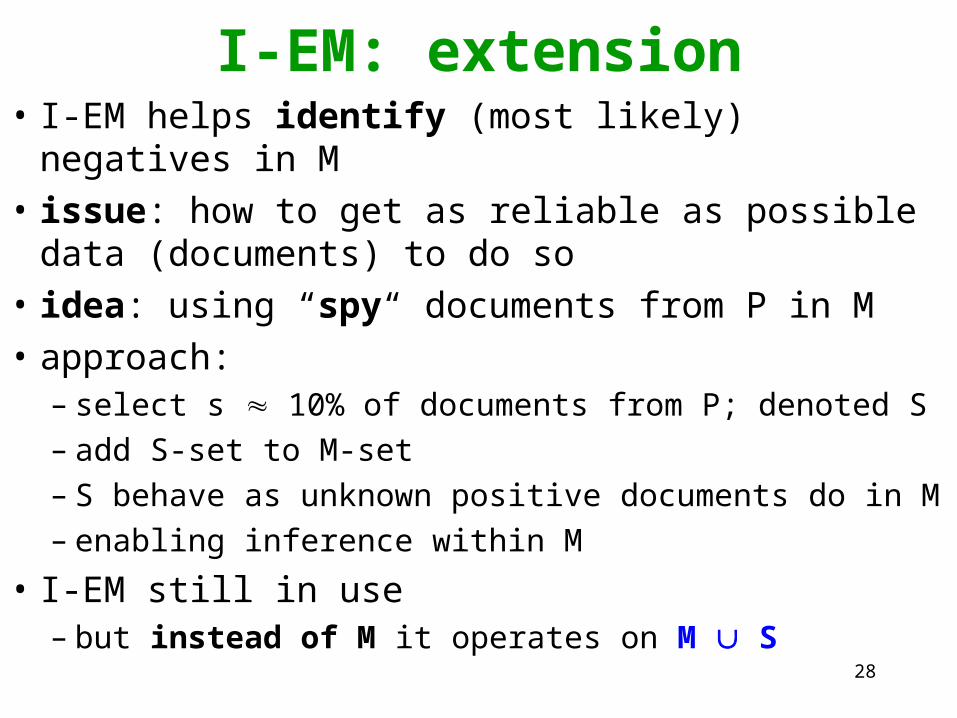
I-EM: extension• I-EM helps identify (most likely) negatives in M

• issue: how to get as reliable as possible data (documents) to do so

• idea: using “spy“ documents from P in M

• approach:– select s 10% of documents from P; denoted S– add S-set to M-set– S behave as unknown positive documents do in M– enabling inference within M

• I-EM still in use– but instead of M it operates on M S

29

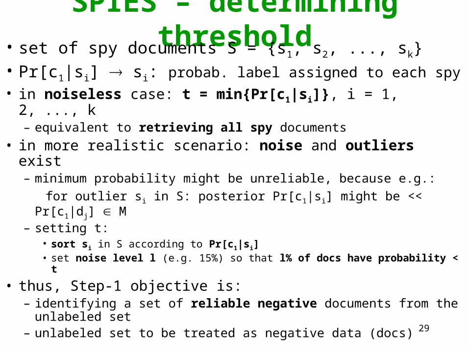
SPIES – determining threshold• set of spy documents S = {s1, s2, ..., sk}

• Pr[c1|si] si: probab. label assigned to each spy

• in noiseless case: t = min{Pr[c1|si]}, i = 1, 2, ..., k– equivalent to retrieving all spy documents

• in more realistic scenario: noise and outliers exist– minimum probability might be unreliable, because e.g.:

for outlier si in S: posterior Pr[c1|si] might be << Pr[c1|dj] M– setting t:

• sort si in S according to Pr[c1|si]• set noise level l (e.g. 15%) so that l% of docs have probability < t

• thus, Step-1 objective is:– identifying a set of reliable negative documents from the

unlabeled set– unlabeled set to be treated as negative data (docs)

30

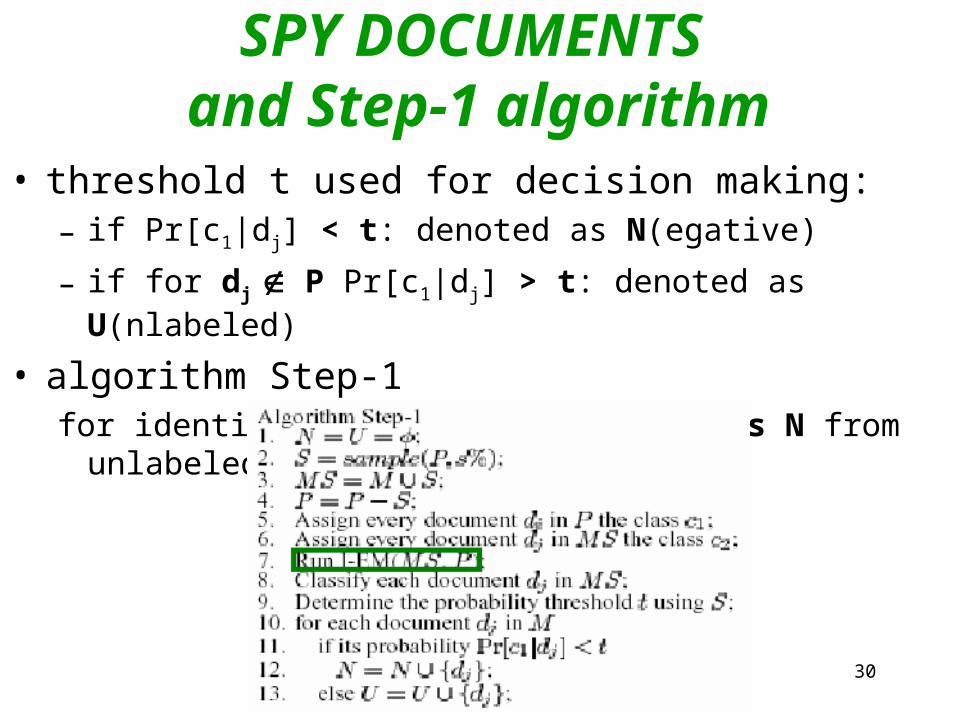
SPY DOCUMENTS and Step-1 algorithm

• threshold t used for decision making:– if Pr[c1|dj] < t: denoted as N(egative)

– if for dj P Pr[c1|dj] > t: denoted as U(nlabeled)

• algorithm Step-1 for identifying most likely negatives N from unlabeled U set

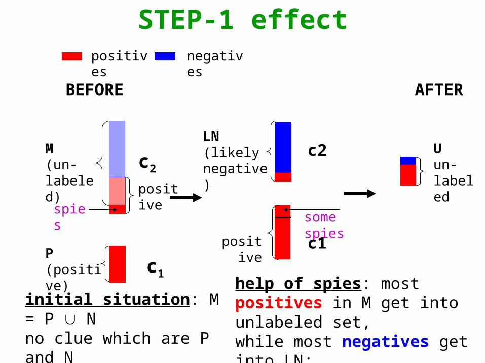
positives negatives

LN(likelynegative)

positive

M(un-labeled)

P(positive)

positive

STEP-1 effect

some spiesspies

c1

c2

c2

c1

Uun-labeled

initial situation: M = P Nno clue which are P and Nspies from P added to M

help of spies: most positives in M get into unlabeled set,while most negatives get into LN;purity of LN higher than that of M

BEFORE AFTER

32

STEP-2: building and selecting final classifier

• EM still in use, but now with P, LN and U

• algorithm proceeds as follows:1. put all spies S back to P (where they were before)

2. diP: c1 (i.e. Pr[c1|di] = 1); (fixed thru iterations)

3. djLN: c2 (i.e. Pr[c2|dj] = 1); (changing thru EM)

4. dkU: initially assigned no label (will be after EM(1))

5. run EM using P, LN and U until it converges

• final classifier is produced when EM stops

• all these constitutes S-EM (spy EM)

33

STEP-2: comments• probabilities of sets U and LN are allowed to

change

• set U participates in EM since EM(2) on with its documents assigned probab. labels Pr[c1|dk]

• experimenting with a = 5%, 10% or 20% gave similar results; why?

• for the parameter a (% used for creating LN):

when within a range of approximately 5%-20%: if too many positives in LN, then

EM corrects it slowly adding them to positives

34

STEP-1 AND STEP-2 SUMMARY

• Step 1: Identifying a set of reliable negative documents from the unlabeled set. The unlabeled set is treated as negative data.

• Step 2: Building and selecting a classifier, consists of two sub-steps:

a) building a set of classifiers by iteratively applying a classification algorithm; the EM algorithm is used again.

b) selecting a good classifier from the set of classifiers constructed above; this sub-step may be called "catching a good classifier".

35

SELECTING CLASSIFIER• as said, EM is prone to local maxima trap

• if a local maximum separates the two classes well: no problem (or problem solved)

• otherwise (i.e. positives and negatives consist of many clusters each) the data may be not separable

• remedy: stop iterating of EM at some point

• what point?

36

SELECTING CLASSIFIER continued

• eq. (2) can be helpful: error probability Pr[f(X) Y] = Pr[f(X) = 1] - Pr[Y = 1] + 2Pr[f(X) = 0|Y = 1]Pr[Y = 1]

• it can be shown that knowing the component PrM[Y = c1] allows us to estimate the error

• method: estimating the change of the probability error between iterations i and i+1

i = can be computed (formula in 4.5 of the paper)

• if i > 0 for the first time, then i-th classifier produced is the last to add (no need to proceed beyond i)

37

EXPERIMENTAL DATA described

• two large document corpora

• 30 datasets created– e.g. 20 newsgroups subdivided into 4 groups

• all headers removed

– e.g. WebKB (CS depts.) subdivided into 7 categories

• objective:– recovering positive documents placed into mixed

sets

• no need to separate test set (from training set)– unlabeled mixed set serves as the test set

38

DATA description cont.• for each experiment:

– dividing full positive set into two subsets: P and R– P: positive set used in the algorithm with a% of the

full positive set– R: set of remaining documents with b% have been

put into negative set M (not all in R put to M)– belief: in reality M is large and has a small

proportion of positive documents

• parameters a and b have been varied to cover different scenarios

39

EXPERIMENTAL RESULTS• techniques used

NB-C: applied directly to P (c1) and M(c2) to built classifier to be applied to classify data in set M

I-EM: applies EM-A to P and M as long as converges (no spy yet); final classifier to be applied to M to identify its positives

S-EM: spies used to re-initialize I-EM to build the final classifier; threshold t used

40

RESULTS cont.• Table 1: 30 results for diferent parametrs a, b• Table 2: summary of averages for other a, b settings

– precision F = 2pr/(p+r), where p, r are and recall, respectively

– S-EM outperforms NB and I-EM in F dramatically– accuracy (of a classifier) A = c/(c+1) , where c, i are

numbers of correct and incorrect decisions, respectively– S-EM outperforms NB and I-EM in A as well

• comment: datasets skewed (positives are only a small fraction), thus A is not a reliable measure of classifier’s performance

41

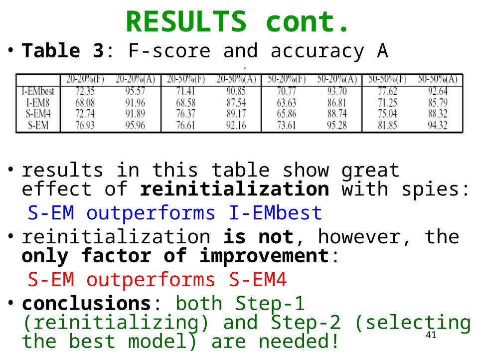
RESULTS cont.• Table 3: F-score and accuracy A

• results in this table show great effect of reinitialization with spies: S-EM outperforms I-EMbest

• reinitialization is not, however, the only factor of improvement:S-EM outperforms S-EM4

• conclusions: both Step-1 (reinitializing) and Step-2 (selecting the best model) are needed!

42

REFERENCES other than in the paper

http://www.cs.uic.edu/~liub/LPU/LPU-download.html

http://www.ant.uni-bremen.de/teaching/sem/ws02_03/slides/em_mud.pdf

http://www.mcs.vuw.ac.nz/~vignaux/docs/Adams_NLJ.html

http://plato.stanford.edu/entries/bayes-theorem/

http://www.math.uiuc.edu/~hildebr/361/cargoat1sol.pdf

http://jimvb.home.mindspring.com/monthall.htm

http://www2.sjsu.edu/faculty/watkins/mhall.htm

http://www.aei-potsdam.mpg.de/~mpoessel/Mathe/3door.html

http://216.239.37.104/search?q=cache:aKEOiHevtE0J:ccrma-www.stanford.edu/~jos/bayes/Bayesian_Parameter_Estimation.html+bayes+likelihood&hl=pl&ie=UTF-8&inlang=pl

THANK YOU