Partially-Latent Class Models (pLCM) for Case-Control ... · Partially-Latent Class Models (pLCM) for Case-Control Studies of Childhood Pneumonia Etiology ... analysis of the motivating

Partially-Latent Class Models (pLCM) for Case-Control

Studies of Childhood Pneumonia Etiology

Zhenke Wu

Department of Biostatistics, Johns Hopkins University, Baltimore, MD 21205, USA

Email: [email protected]

Maria Deloria-Knoll

Department of International Health, Johns Hopkins University, Baltimore, MD 21205, USA

Laura L. Hammitt

Department of International Health, Johns Hopkins University, Baltimore, MD 21205, USA

Scott L. Zeger

Department of Biostatistics, Johns Hopkins University, Baltimore, MD 21205, USA

for the PERCH Core Team

Summary. In population studies on the etiology of disease, one goal is the estimation of

the fraction of cases attributable to each of several causes. For example, pneumonia is a

clinical diagnosis of lung infection that may be caused by viral, bacterial, fungal, or other

pathogens. The study of pneumonia etiology is challenging because directly sampling from

the lung to identify the etiologic pathogen is not standard clinical practice in most settings. In-

stead, measurements from multiple peripheral specimens are made. This paper introduces

the statistical methodology designed for estimating the population etiology distribution and

the individual etiology probabilities in the Pneumonia Etiology Research for Child Health

(PERCH) study of 9, 500 children for 7 sites around the world. We formulate the scientific

problem in statistical terms as estimating the mixing weights and latent class indicators un-

der a partially-latent class model (pLCM) that combines heterogeneous measurements with

different error rates obtained from a case-control study. We introduce the pLCM as an ex-

tension of the latent class model. We also introduce graphical displays of the population

data and inferred latent-class frequencies. The methods are tested with simulated data, and

then applied to PERCH data. The paper closes with a brief description of extensions of the

pLCM to the regression setting and to the case where conditional independence among the

measures is relaxed.

Keywords: Bayesian method; Case-control; Etiology; Latent class; Measurement er-

ror; Pneumonia

arX

iv:1

411.

5774

v1 [

stat

.AP]

21

Nov

201

4

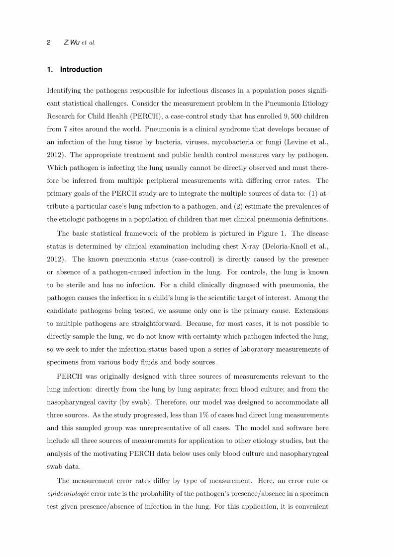
2 Z.Wu et al.

1. Introduction

Identifying the pathogens responsible for infectious diseases in a population poses signifi-

cant statistical challenges. Consider the measurement problem in the Pneumonia Etiology

Research for Child Health (PERCH), a case-control study that has enrolled 9, 500 children

from 7 sites around the world. Pneumonia is a clinical syndrome that develops because of

an infection of the lung tissue by bacteria, viruses, mycobacteria or fungi (Levine et al.,

2012). The appropriate treatment and public health control measures vary by pathogen.

Which pathogen is infecting the lung usually cannot be directly observed and must there-

fore be inferred from multiple peripheral measurements with differing error rates. The

primary goals of the PERCH study are to integrate the multiple sources of data to: (1) at-

tribute a particular case’s lung infection to a pathogen, and (2) estimate the prevalences of

the etiologic pathogens in a population of children that met clinical pneumonia definitions.

The basic statistical framework of the problem is pictured in Figure 1. The disease

status is determined by clinical examination including chest X-ray (Deloria-Knoll et al.,

2012). The known pneumonia status (case-control) is directly caused by the presence

or absence of a pathogen-caused infection in the lung. For controls, the lung is known

to be sterile and has no infection. For a child clinically diagnosed with pneumonia, the

pathogen causes the infection in a child’s lung is the scientific target of interest. Among the

candidate pathogens being tested, we assume only one is the primary cause. Extensions

to multiple pathogens are straightforward. Because, for most cases, it is not possible to

directly sample the lung, we do not know with certainty which pathogen infected the lung,

so we seek to infer the infection status based upon a series of laboratory measurements of

specimens from various body fluids and body sources.

PERCH was originally designed with three sources of measurements relevant to the

lung infection: directly from the lung by lung aspirate; from blood culture; and from the

nasopharyngeal cavity (by swab). Therefore, our model was designed to accommodate all

three sources. As the study progressed, less than 1% of cases had direct lung measurements

and this sampled group was unrepresentative of all cases. The model and software here

include all three sources of measurements for application to other etiology studies, but the

analysis of the motivating PERCH data below uses only blood culture and nasopharyngeal

swab data.

The measurement error rates differ by type of measurement. Here, an error rate or

epidemiologic error rate is the probability of the pathogen’s presence/absence in a specimen

test given presence/absence of infection in the lung. For this application, it is convenient

Partially-latent class models for etiology estimation 3

to categorize measures into three subgroups referred to as “gold”, “silver”, and “bronze”

standard measurements. A gold-standard (GS) measurement is assumed to have both

perfect sensitivity and specificity. Lung aspirate data would have been gold-standard. A

silver-standard (SS) measurement is assumed to have perfect specificity, but imperfect

sensitivity. Culturing bacteria from blood samples (B-cX) is an example of silver-standard

measurements in PERCH. Finally, bronze-standard (BrS) measurements are assumed to

have imperfect sensitivity and specificity. Polymerase chain reaction (PCR) evaluation of

bacteria and viruses from nasopharyngeal samples is an example.

In the PERCH study, both SS and BrS measurements are available for all cases. BrS,

but not SS measures are available for controls. Our goal was to develop a statistical model

that combines GS and SS measurements from cases, with BrS data from cases and controls

to estimate the distribution of pathogens in the population of pneumonia cases, and the

conditional probability that each of the J pathogens is the primary cause of an individual

child’s pneumonia given her or his set of measurements. Even in applications where GS

data is not available, a flexible modeling framework that can accommodate GS data is

useful for both the evaluation of statistical information from BrS data (Section 3) and the

incorporation of GS data if it becomes available as measurement technology improves.

Latent class models (LCM) (Goodman, 1974) have been successfully used to integrate

multiple diagnostic tests or raters’ assessments to estimate a binary latent status for all

study subjects (Hui and Walter, 1980; Qu and Hadgu, 1998; Albert et al., 2001; Albert

and Dodd, 2008). In the LCM framework, conditional distributions of measurements given

latent status are specified. Then the marginal likelihood of the multivariate measurements

are maximized as a function of the disease prevalence, sensitivities and specificities. This

framework has also been extended to infer ordinal latent status (Wang et al., 2011).

There are three salient features of the PERCH childhood pneumonia problem that

require extension of the typical LCM approach. First, we have partial knowledge of the

latent lung state for some subjects as a result of the case-control design. In the standard

LCM approach, the study population comprises subjects with completely unknown class

membership. In this study, controls are known to have no pathogen infecting the lung.

Also, were gold standard measurements available from the lung for some cases, their latent

variable would be directly observed. As the latent state is known for a non-trivial subset of

the study population, we refer to this model as a partially-Latent Class Model or pLCM.

Second, in most LCM applications, the number of observed measurements on a subject

is much larger than the number of latent state categories. Here, the number of observations

4 Z.Wu et al.

is of the same order as the number of categories that the latent status can assume. For

example, if we consider only the PERCH study BrS data, we simultaneously observe the

presence/absence of each member from a list of possible pathogens for each child. Even

with additional control data, the larger number of latent categories of latent status leads

to weak model identifiability as is discussed in more detail in Section 2.1.

Lastly, measurements with differing error rates (i.e. GS, SS, BrS) need to be integrated.

Note that the modeling framework introduced here is general and can be applied to studies

where multiple BrS measurements are available, each with a different set of error rates.

Understanding the relative value of each level of measurements is important to optimally

invest resources into data collection (number of subjects, type of samples) and laboratory

assays. An important goal is therefore to estimate the relative information from each type

of measurements about the population and individual etiology distributions.

Albert and Dodd (2008) studied a model where some subjects are selected to verify

their latent status (i.e. collect GS measurements) with the probability of verification

either depending on the previous test results or being completely at random. They showed

GS data can make model estimates more robust to model misspecifications. We further

quantify how much GS data reduces the variance of model parameter estimates for design

purposes. Also, they considered binary latent status and did not have available control

data. Another related literature that uses both GS and BrS data is on verbal autopsy (VA)

in the setting where no complete vital registry system is established in the community

(King and Lu, 2008). Quite similar to the goal of inferring pneumonia etiology from lab

measurements, the VA goal is to infer the cause of death from a pre-specified list by asking

close family members questions about the presence/absence of several symptoms. King

and Lu (2008) proposed estimating the cause-of-death distribution in a community using

data on dichotomous symptoms and GS data from the hospital where cause-of-death and

symptoms are both recorded. However, their method involves nonparametric and requires

a sizable sample of GS data, especially when the number of symptoms is large. In addition,

a key difference between VA and most infectious disease etiology studies is that the VA

studies are by definition case-only.

Another approach previously used with case and control data is to perform logistic

regression of case status on laboratory measurements and then to calculate point estimates

of population attributable risks for each pathogen (Bruzzi et al., 1985; Blackwelder et al.,

2012). This method does not account for imperfect laboratory measurements and cannot

use GS or SS data if available. Also, the population attributable fraction method assigns


zero etiology for the subset of pathogens that have estimated odds ratios smaller than 1,

without taking account of the statistical uncertainty for the odds ratio estimates.

In this paper, we define and apply a partially-latent class model (pLCM) to incorpo-

rate these three features: known infection status for controls; a large number of latent

classes; and multiple types of measurements. We use a hierarchical Bayesian formulation

to estimate: (1) the population etiology distribution or etiology fraction —the frequency

with which each pathogen “causes” clinical pneumonia in the case population; and (2) the

individual etiology probabilities—the probabilities that a case is “caused” by each of the

candidate pathogens, given observed specimen measurements for that individual.

In Section 4, to facilitate communications with scientists, we introduce graphical dis-

plays that put data, model assumptions, and results together. They enable the scientific

investigators to better understand the various sources of evidence from data and their

contribution to the final etiology estimates.

The remainder of this paper proceeds as follows. In section 2, we formulate the pLCM

and the Gibbs sampling algorithms for implementation. In Section 3, we evaluate our

method through simulations tailored for the childhood pneumonia etiology study. Section

4 presents the analysis of PERCH data. Lastly, Section 5 concludes with a discussion

of results and limitations, a few natural extensions of the pLCM also motivated by the

PERCH data, as well as future directions of research.

2. A partially-latent class model for multiple indirect measurements

We develop pLCM to address two characteristics of the motivating pneumonia problem: (1)

a partially-latent state variable because the pathogen infection status is known for controls

but not cases; and (2) multiple categories of measurements with different error rates across

classes. As shown in Figure 1, let ILi , taking values in {0, 1, 2, ...J}, represent the true

state of child i’s lung (i = 1, ..., N) where 0 represents no infection (control) and ILi = j,

j = 1, ..., J , represents the jth pathogen from a pre-specified cause-of-pneumonia list that

is assumed to be exhaustive. ILi is the scientific target of inference for individual diagnosis.

Let MSi represent the J × 1 vector of binary indicators of the presence/absence of each

pathogen in the measurement at site S, where, in our childhood pneumonia etiology study

S can be nasopharyngeal (NP), blood (B), or lung (L). Let mSi be the actual observed

values. In the following, we replace S with BrS, SS, or GS, because they correspond to

the measurement types at NP, B, and L, respectively.

Let Yi = yi ∈ {0, 1} represent the indicator of whether child i is a healthy control or a

6 Z.Wu et al.

clinically diagnosed case. Note ILi = 0 given Yi = 0. To formalize the pLCM, we define

three sets of parameters:

• π = (π1, ..., πJ)′ , the vector of compositional probabilities for each of J pathogen

causes, that is, Pr(ILi = j | Yi = 1,π), j = 1, ..., J ;

• ψSj = Pr(MSij = 1|ILi = 0), the false positive rate (FPR) for measurement j (j =

1, ..., J) at site S. Note that The FPRs {ψSj }Jj=1 can be estimated from the control

data at site S, because ILi = 0 denotes that the ith subject has no infection in the

lung, i.e. a control;

• θSj = Pr(MSij = 1|ILi = j), the true positive rate (TPR) for measurement j at site S

for a person whose lung is infected by pathogen j, j = 1, ...J .

We further let ψS = (ψS1 , ..., ψSJ )′ and θS = (θS1 , ..., θ

SJ )′. Using these definitions, we have

FPR ψGSj = 0 and TPR θGS

j = 1 for GS measurements, so that MGSij = 1 if and only

if ILi = j, j = 1, ..., J (perfect sensitivity and specificity). For SS measurements, FPR

ψSSj = 0 so that MSS

j = 0 if ILi 6= j (perfect specificity).

We formalize the model likelihood for each type of measurement. We first describe the

model for BrS measurement MBrS for a control or a case. For control i, positive detection

of the jth pathogen is a false positive representation of the non-infected lung. Therefore,

we assume MBrSij | ψBrS ∼ Bernoulli(ψSj ), j = 1, ..., J , with conditional independence, or

equivalently,

P 0,BrSi = Pr(MBrS

i = m | ψBrS ) =

J∏j=1

(ψBrSj

)mj(1− ψBrS

j

)1−mj, (1)

where m = mBrSi . For a case infected by pathogen j, the positive detection rate for the

jth pathogen in BrS assays is θBrSj . Since we assume a single cause for each case, detection

of pathogens other than j will be false positives with probability equal to FPR as in

controls: ψBrSl , l 6= j. This nondifferential misclassification across the case and control

populations is the essential assumption of the latent class approach because it allows us to

borrow information from control BrS data to distinguish the true cause from background

colonization. We further discuss it in the context of the pneumonia etiology problem in

the final section. Then,

P 1,BrSi = Pr(MBrS

i = m | π,θBrS ,ψBrS )

=

J∑j=1

πj ·(θBrSj

)mj(1− θBrS

j

)1−mj∏l 6=j

(ψBrSl

)ml(1− ψBrS

l

)1−ml, (2)


is the likelihood contributed by BrS measurements from case i, where m = mBrSi .

Similarly, likelihood contribution from case i’s SS measurements can be written as

P 1,SSi = Pr(MSS

i = m | π,θSS ) =

J ′∑j=1

πj ·(θSSj

)mj(1− θSS

j )1−mj1{∑J′l=1ml≤1}, (3)

for m = mSSi , noting the perfect specificity of SS measurements, where J ′ ≤ J represents

the number of actual SS measurements on each case, and θSS =(θSS1 , ...θSS

J ′). SS measure-

ments only test for a subset of all J pathogens, e.g., blood culture only detects bacteria

and J ′ is the number of bacteria that are potential causes. Finally, for completeness, GS

measurement is assumed to follow a multinomial distribution with likelihood:

P 1,GSi = Pr

(MGSi = m | π

)=

J∏j=1

π1{mj=1}j 1{

∑j mj=1}, (4)

where m = mGSi , and 1{·} is the indicator function and equals one if the statement in {·}

is true; otherwise, zero.

Let δi be the binary indicator of a case i having GS measurements; it equals 1 if the

case has available GS data and 0 otherwise. Combining likelihood components (1)—(4),

the total model likelihood for BrS, SS, and GS data across independent cases and controls

is

L(γ;D) =∏i:Yi=0

P 0,BrSi

∏i:Yi=1,δi=1

P 1,BrSi · P 1,SS

i · P 1,GSi

∏i:Yi=1,δi=0

P 1,BrSi · P 1,SS

i , (5)

where γ = (θBrS ,ψBrS ,θSS ,π)′ stacks all unknown parameters, and data D is{{mBrS

i

}i:Yi=0

}∪{{mBrS

i ,mGSi ,mSS

i

}i:Yi=1,δi=1

}∪{{mBrS

i′′ ,mSSi′′}i′′ :Y

i′′=1,δ

i′′=0

}collects all the available measurements on study subjects. Our primary statistical goal

is to estimate the posterior distribution of the population etiology distribution π, and to

obtain individual etiology (IL∗ ) prediction given a case’s measurements.

To enable Bayesian inference, prior distributions on model parameters are specified as

follows: π ∼ Dirichlet(a1, . . . , aJ), ψBrSj ∼ Beta(b1j , b2j), θ

BrSj ∼ Beta(c1j , c2j), j = 1, ..., J ,

and θSSj ∼ Beta(d1j , d2j), j = 1, ..., J ′. Hyperparameters for etiology prior, a1, ..., aJ , are

usually 1s to denote equal and non-informative prior weights for each pathogen if expert

prior knowledge is unavailable. The FPR for the jth pathogen, ψBrSj , generally can be well

estimated from control data, thus b1j = b2j = 1 is the default choice. For TPR parameters

θBrSj and θSS

j , if prior knowledge on TPRs is available, we choose (c1j , c2j) so that the

2.5% and 97.5% quantiles of Beta distribution with parameter (c1j , c2j) match the prior

minimum and maximum TPR values elicited from pneumonia experts . Otherwise, we

8 Z.Wu et al.

use default value 1s for the Beta hyperparameters. Similarly we choose values of (d1j , d2j)

either by prior knowledge or default values of 1. We finally assume prior independence

of the parameters as [γ] = [π][ψBrS ][θBrS ][θSS ], where [A] represents the distribution of

random variable or vector A. These priors represent a balance between explicit prior

knowledge about measurement error rates and the desire to be as objective as possible for

a particular study. As described in the next section, the identifiability constraints on the

pLCM require specifying a reasonable subset of parameter values to identify parameters

of greatest scientific interest.

2.1. Model identifiability

Potential non-identifiability of LCM parameters is well-known (Goodman, 1974). For

example, an LCM with four observed binary indicators and three latent classes is not

identifiable despite providing 15 degree-of-freedom to estimate 14 parameters (Goodman,

1974). In principle, the Bayesian framework avoids the non-identifiability problem in

LCMs by incorporating prior information about unidentified parameter subspaces (e.g.,

Garrett and Zeger (2000)). Many authors point out that the posterior variance for non-

identifiable parameters does not decrease to zero as sample size approaches infinity (e.g.,

Kadane (1974); Gustafson et al. (2001); Gustafson (2005)). Even when data are not fully

informative about a parameter, an identified set of parameter values consistent with the

observed data shall, can nevertheless, be valuable in a complex scientific investigation

(Gustafson, 2009) like PERCH.

When GS data is available, the pLCM is identifiable; when it is not, the two sets

of parameters, π and {θBrSj }Jj=1 are not both identified and prior knowledge must be

incorporated. Here we restrict attention to the scenario with only BrS data for simplicity

but similar arguments pertain to the BrS + SS scenario. The problem can be understood

from the form of the positive measurement rates for pathogens among cases. In the pLCM

likelihood for the BrS data (only retaining components in (5) with superscripts BrS ), the

positive rate for pathogen j is a convex combination of the TPR and FPR:

Pr(MBrSij = 1 | πj , θBrS

j , ψBrSj

)= πjθ

BrSj + (1− πj)ψBrS

j , (6)

where the left-hand side of the above equation can be estimated by the observed positive

rate of pathogen j among cases. Although the control data provide ψBrSj estimates, the

two parameters, πj and θBrSj , are not both identified. GS data, if available, identifies πj

and resolves the lack of identifiability. Otherwise, we need to incorporate prior scientific

information on one of them, usually the TPR (θBrSj ). In PERCH, prior knowledge about


θBrSj is obtained from infectious disease and laboratory experts (Murdoch et al., 2012)

based upon vaccine probe studies (Cutts et al., 2005; Madhi et al., 2005). If the observed

case positive rate is much higher than the rate in controls (ψBrSj ), only large values of TPR

(θBrSj ) are supported by the data making etiology estimation more precise (Section 2.2).

The full model identification can be generally characterized by inspecting the Jacobian

matrix of the transformation F from model parameters γ to the distribution p of the ob-

servables, p = F (γ). Let γ = (θBrS ,ψBrS , π1, ..., πJ−1)′ represent the 3J − 1-dimensional

unconstrained model parameters. The pLCM defines the transformation (p1,p0)′ = F (γ),

where p1 and p0 are the two contingency probability distributions for the BrS measure-

ments in the case and control populations, each with dimension 2J − 1. It can be shown

that the Jacobian matrix has J − 1 of its singular values being zero, which means model

parameters γ are not fully identified from the data. The FPRs (ψBrSj , j = 1, ..., J) in pLCM

are, however, identifiable parameters that can be estimated from control data. Therefore,

pLCM is termed partially identifiable (Jones et al., 2010).

2.2. Parameter estimation and individual etiology prediction

The parameters in likelihood (5) include the population etiology distribution (π), TPRs

and FPRs for BrS measurements (ψBrS and θBrS ), and TPRs for SS measurements (θSS ).

The posterior distribution of these parameters can be estimated by constructing approxi-

mating samples from the joint posterior via a Markov chain Monte Carlo (MCMC) Gibbs

sampler. The full conditional distributions for the Gibbs sampler are detailed in Section

A of the supplementary material.

We develop a Gibbs sampler with two essential steps:

(i) Multinomial sampling of lung infection state among cases:

ILi | π, Yi = 1 ∼ Multinomial(π);

(ii) Measurement stage given lung infection state:

MBrSij | ILi ,θBrS ,ψBrS ∼ Bernoulli

(1{ILi =j}θ

BrSj +

(1− 1{ILi =j}

)ψBrSj

), j = 1, ..., J ,

conditionally independent.

This is readily implemented using freely available software WinBUGS 1.4. In the ap-

plication below, convergence was monitored using auto-correlations, kernel density plots,

and Brooks-Gelman-Rubin statistics (Brooks and Gelman, 1998) of the MCMC chains.

The statistical results below are based on 10, 000 iterations of burn-in followed by 50, 000

production samples from each of three parallel chains.

10 Z.Wu et al.

The Bayesian framework naturally allows individual within-sample classification (in-

fection diagnosis) and out-of-sample prediction. This section describes how we calculate

the etiology probabilities for an individual with measurements m∗. We focus on the more

challenging inference scenario when only BrS data are available; the general case follows

directly.

The within-sample classification for case i is based on the posterior distribution of

latent indicators given the observed data, i.e. Pr(ILi = j | D), j = 1, ..., J , which can be

obtained by averaging along the cause indicator (ILi ) chain from MCMC samples. For a

case with new BrS measurements m∗, we have

Pr(ILi = j |m∗,D) =

∫Pr(ILi = j |m∗,γ) Pr(γ |m∗,D)dγ, j = 1, ...J, (7)

where the second factor in the integrand can be approximated by the posterior distribution

given current data, i.e., Pr(γ | D). For the first term in the integrand, we explicitly obtain

the model-based, one-sample conditional posterior distribution, Pr(ILi = j | m∗,γ) =

πj`j(m∗;γ)

/∑m πrm

`m(m∗;γ), j = 1, ..., J , where

`m(m∗;γ) =(θBrSj

)m∗j (1− θBrS

j

)1−m∗j ∏l 6=j

(ψBrSl

)m∗l (1− ψBrS

l

)1−m∗lis the mth mixture component likelihood function evaluated at m∗. The log relative

probability of ILi = j versus ILi = l is

Rjl = log

(πjπl

)+ log

(θBrSj

ψBrSj

)m∗j (1− θBrS

j

1− ψBrSj

)1−m∗j

+ log

{(ψBrSl

θBrSl

)m∗l (1− ψBrSl

1− θBrSl

)1−m∗l}.

The form of Rjl informs us about what is required for correct diagnosis of an individual.

Suppose ILi = j, then averaging over m∗, we have E[Rjl] = log (πj/πl) + I(θBrSj ;ψBrS

j ) +

I(ψBrSl ; θBrS

l ), where I(v1; v2) = v1 log(v1/v2) + (1− v1) log ((1− v1)/(1− v2)) is the infor-

mation divergence (Kullback, 2012) that represents the expected amount of information

in m∗j ∼ Bernoulli(v1) for discriminating against m∗j ∼ Bernoulli(v2). If v1 = v2, then

I(v1; v2) = 0. The form of E[Rjl] shows that there is only additional information from BrS

data about an individual’s etiology in the person’s data when there is a difference between

θBrSj and ψBrS

j , j = 1, ..., J .

Following equation (7), we average Pr(ILi = j | m∗,γ) over MCMC iterations to

obtain individual prediction for the jth pathogen, pij , with γ replaced by its simulated

values γ∗ at each iteration. Repeating for j = 1, ..., J , we obtain a J probability vector,


pi = (pi1, ..., piJ)′, that sums to one. This scheme is especially useful when a newly

examined case has a BrS measurement pattern not observed in D, which often occurs when

J is large. The final decisions regarding which pathogen to treat can then be based upon

pi. In particular, the pathogen with largest posterior value might be selected. It is Bayes

optimal under mean misclassification loss. Individual etiology predictions described here

generalize the positive/negative predictive value (PPV/NPV) from single to multivariate

binary measurements and can aid diagnosis of case subjects under other user-specified

misclassification loss functions.

3. Simulation for three pathogens case with GS and BrS data

To demonstrate the utility of the pLCM for studies like PERCH, we simulate BrS data

sets with 500 cases and 500 controls for three pathogens, A, B, and C using known

pLCM specifications. We focus on three states to facilitate viewing of the π estimates

and individual predictions in the 3-dimensional simplex S2. We use the ternary dia-

gram (Aitchison, 1986) representation where the vector π = (πA, πB, πC)′ is encoded

as a point with each component being the perpendicular distance to one of the three

sides. The parameters involved are fixed at TPR = θ = (θA, θB, θC)′ = (0.9, 0.9, 0.9)′,

FPR = ψ = (ψA, ψB, ψC)′ = (0.6, 0.02, 0.05)′, and π = (πA, πB, πC)′ = (0.67, 0.26, 0.07)′.

We focus on BrS and GS data here and have dropped the “BrS ” superscript on the pa-

rameters for simplicity. We further let the fraction of cases with GS measurements (∆)

be either 1% as in PERCH or 10%. Although GS measurements are rare in the PERCH

study, we investigate a large range of ∆ to understand in general how much statistical

information is contained in BrS measurements relative to GS measurements.

For any given data set, three distinct subsets of the data can be used: BrS-only, GS-only,

and BrS+GS, each producing its posterior mean of π, and 95% credible region (Bayesian

confidence region) by transformed Gaussian kernel density estimator for compositional

data (Chacon et al., 2011). To study the relative importance of the GS and BrS data, the

primary quantity of interest in the simulations is the relative sizes of the credible regions

for each data mix. Here, we use uniform priors on θ, ψ, and Dirichlet(1, ..., 1) prior for π.

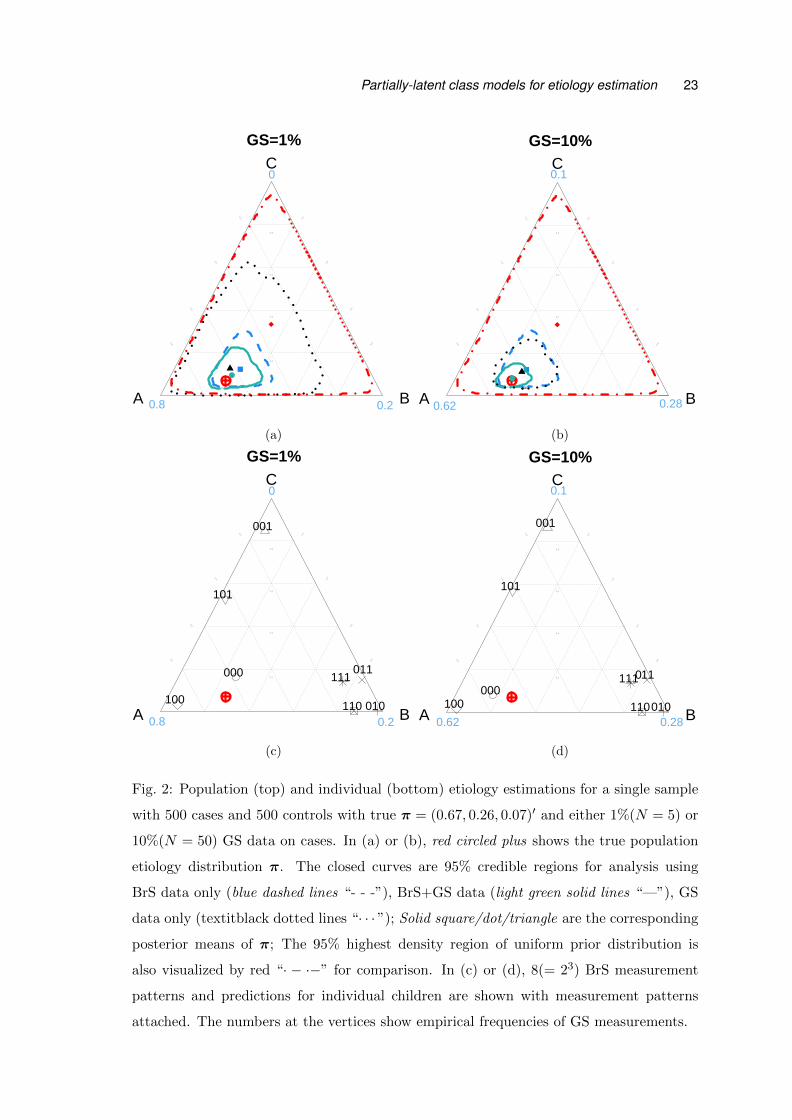
The results are shown in Figure 2.

First, in Figures 2a (1% GS) and 2b (10% GS), each region covers the true etiology π.

In data not shown here, the nominal 95% credible regions covers slightly more than 95%

of 200 simulations. Credible regions narrow in on the truth as we combine BrS and GS

data, and as the fraction of subjects with GS data (∆) increases. Also, the posterior mean

12 Z.Wu et al.

from the BrS+GS analysis is an optimal balance of information contained in the GS and

BrS data.

Using the same simulated data sets, Figures 2c and 2d also show individual etiology

predictions for each of the 8(= 23) possible BrS measurements (mA,mB,mC)′,mj = 0, 1,

obtained by the methods from Section 2.2. Consider the example of a newly enrolled

case without GS data and with no pathogen observed in her BrS data: m = (0, 0, 0)′.

Suppose she is part of a case population with 10% GS data. In the case illustrated in

Figure 2d, her posterior predictive distribution has highest posterior probability (0.76)

on pathogen A reflecting two competing forces: the FPRs that describe background colo-

nization (colonization among the controls) and the population etiology distribution. Given

other parameters, m = (0, 0, 0)′ gives the smallest likelihood for ILi = A because of its high

background colonization rate (FPR ψA = 0.6). However, prior to observing (0, 0, 0)′, πA

is well estimated to be much larger than πB and πC . Therefore the posterior distribution

for this case is heavily weighted towards pathogen A.

Because it is rare to observe pathogen B in a case whose pneumonia is not caused by

B, for a case with observation (1, 1, 1)′, the prediction favors B. Although B is not the

most prevalent cause among cases, the presence of B in the BrS measurements gives the

largest likelihood when ILi = B. For any measurement pattern with a single positive, the

case is always classified into that category in this example.

Most predictions are stable with increasing gold-standard percentage, ∆. Only 000

cases have predictions that move from near the center to the corner of A. This is mainly

because that TPR θ and etiology fractions π are not as precisely estimated in GS-scarce

scenarios relative to GS-abundant ones. Averaging over a wider range of θ and π produces

000 case predictions that are ambiguous, i.e. near the center. As ∆ increases, parameters

are well estimated, and precise predictions result.

4. Analysis of PERCH data

The Pneumonia Etiology Research for Child Health (PERCH) study is an on-going stan-

dardized and comprehensive evaluation of etiologic agents causing severe and very severe

pneumonia among hospitalized children aged 1-59 months in seven low and middle income

countries (Levine et al., 2012). The study sites include countries with a significant burden

of childhood pneumonia and a range of epidemiologic characteristics. PERCH is a case-

control study that has enrolled over 4, 000 patients hospitalized for severe or very severe

pneumonia and over 5, 000 controls selected randomly from the community frequency-


matched on age in each month. More details about the PERCH design are available in

Deloria-Knoll et al. (2012).

To analyze PERCH data with the pLCM model, we have focused on preliminary data

from one site with good availability of both SS and BrS laboratory results (no missing-

ness). Final analyses of all 7 countries will be reported elsewhere upon study completion.

Included in the current analysis are BrS data (nasopharyngeal specimen with PCR de-

tection of pathogens) for 432 cases and 479 frequency-matched controls on 11 species of

pathogens (7 viruses and 4 bacteria; representing a subset of pathogens evaluated; their

abbreviations shown on the right margin in Figure 3, and full names in Section B of the

supplementary material), and SS data (blood culture results) on the 4 bacteria for only

the cases.

In PERCH, prior scientific knowledge of measurement error rates is incorporated into

the analysis. Based upon microbiology studies (Murdoch et al., 2012), the PERCH in-

vestigators selected priors for the TPRs of our BrS measurements, θBrSj , in the range of

50%− 100% for viruses and 0− 100% for bacteria. Priors for the SS TPRs were based on

observations from vaccine probe studies—randomized clinical trials of pathogen-specific

vaccines where the total number of clinical pneumonia cases prevented by the vaccine

is much larger than the few SS laboratory-confirmed cases prevented. Comparing the

total preventable disease burden to the number of blood culture (SS) positive cases pre-

vented provides information about the TPR of the bacterial blood culture measurements,

θSSj , j = 1, ..., 4. Our analysis used the range 5−15% for the SS TPRs of the four bacteria

consistent with the vaccine probe studies (Cutts et al., 2005; Madhi et al., 2005). We set

Beta priors that match these ranges (Section 2) and assumed Dirichlet(1, ..., 1) prior on

etiology fractions π.

In latent variable models like the pLCM, key variables are not directly observed. It

is therefore essential to picture the model inputs and outputs side-by-side to better un-

derstand the analysis. In this spirit, Figure 3 displays for each of the 11 pathogens, a

summary of the BrS and SS data in the left two columns, along with some of the inter-

mediate model results; and the prior and posterior distributions for the etiology fractions

on the right (rows ordered by posterior means). The observed BrS rates (with 95% con-

fidence intervals) for cases and controls are shown on the far left with solid dots. The

conditional odds ratio contrasting the case and control rates given the other pathogens

is listed with 95% confidence interval in the box to the right of the BrS data summary.

Below the case and control observed rates is a horizontal line with a triangle. From left

14 Z.Wu et al.

to right, the line starts at the estimated false positive rate (FPR, ψBrSj ) and ends at the

estimated true positive rate (TPR, θBrSj ), both obtained from the model. Below the TPR

are two boxplots summarizing its posterior (top) and prior (bottom) distributions for that

pathogen. These box plots show how the prior assumption influences the TPR estimate

as expected given the identifiability constraints discussed in Section 2.1. The triangle on

the line is the model estimate of the case rate to compare to the observed value above

it. As discussed in Section 2.1, the model-based case rate is a linear combination of the

FPR and TPR with mixing fraction equal to the estimated etiology fraction. Therefore,

the location of the triangle, expressed as a fraction of the distance from the FPR to the

TPR, is the model-based point estimate of the etiologic fraction for each pathogen. The

SS data are shown in a similar fashion to the right of the BrS data. By definition, the

FPR is 0.0% for SS measures and there is no control data. The observed rate for the cases

is shown with its 95% confidence interval. The estimated SS TPR (θSSj ) with prior and

posterior distributions is shown as for the BrS data, except that we plot 95% and 50%

credible intervals for SS TPR above its prior 95% and 50% intervals.

On the right side of the display are the marginal posterior and prior distributions of the

etiologic fraction for each pathogen. We appropriately normalized each density to match

the height of the prior and posterior curves. The posterior mean, 50% and 95% credible

intervals are shown above the density.

Figure 3 shows that respiratory syncytial virus (RSV), Streptococcus pneumoniae (PNEU),

rhinovirus (RHINO), and human metapneumovirus (HMPV A B) occupy the greatest

fractions of the etiology distribution, from 15% to 30% each. That RSV has the largest

estimated mean etiology fraction reflects the large discrepancy between case and con-

trol positive rates in the BrS data: 25.1% versus 0.8% (marginal odds ratio 38.5 (95%CI

(18.0, 128.7) ). RHINO has case and control rates that are close to each other, yet its

estimated mean etiology fraction is 16.7%. This is because the model considers the joint

distribution of the pathogens, not the marginal rates. The conditional odds ratio of case

status with RHINO given all the other pathogen measures is estimated to be 1.5 (1.1, 2.1)

as in contrast to the marginal odds ratio close to 1 (0.8, 1.3).

As discussed in Section 2.1, the data alone cannot precisely estimate both the etiologic

fractions and TPRs absent prior knowledge. This is evidenced by comparing the prior and

posterior distributions for the TPRs in the BrS boxes for some pathogens like HMPV A B

and PARA1 (i.e. left hand column of Figure 3). The posteriors are similar to their

priors indicating little else about TPR is learned from the data. The posteriors for some


pathogens making up π (i.e. shown in the right hand column of Figure 3) are likely to be

sensitive to the prior specifications of the TPRs.

We performed sensitivity analyses using multiple sets of priors for the TPRs. At one

extreme, we ignored background scientific knowledge and let the priors on the FPR and

TPR be uniform for both the BrS and SS data. Ignoring prior knowledge about error rates

lowers the etiology estimates of the bacteria PNEU and Staphylococcus aureus (SAUR).

The substantial reduction in the etiology fraction for PNEU, for example, is a result of

the difference in the TPR prior for the SS measurements. In the original analysis (Figure

3), the informative prior on the SS sensitivity (TPR) places 95% mass between 5− 15%.

Hence the model assumes almost 90% of the PNEU infections are being missed in the SS

sampling. When a uniform prior is substituted, the fraction assumed missed is greatly

reduced. For RSV, its posterior mean etiology fraction is stable (29.4% to 30.0%). The

etiology estimates for other pathogens are fairly stable, with changes in posterior means

between −2.3% and 3.4%.

Under the original priors for TPR, PARA1 has an estimated etiologic fraction of 6.4%,

even though it has conditional odds ratio 5.9 (2.6, 15.0). In general, pathogens with larger

conditional odds ratios have larger etiology fraction estimates. But a pathogen also needs

a reasonably high observed case positive rate to be allocated a high etiology fraction. The

posterior etiology fraction estimate of 6.4% for PARA1 results because the prior for the

TPR takes values in the range of 50 − 99%. By Equation (6), the TPR weight in the

convex combination with FPR (around 1.5%) has to be very small to explain the small

observed case rate 5.6%. When a uniform prior is placed on TPR instead, the PARA1

etiology fraction increases to 9.4% with a wider 95% credible interval.

We believe that RHINO’s etiologic fraction may be inflated as a result of its negative

association with RSV among cases. Under the conditional independence assumption of

the pLCM, this dependence can only be explained by multinomial correlation among the

latent cause indicators: ILi = RSV versus ILi = RHINO that is −πRSVπRHINO. There is

strong evidence that RSV is a common cause with a stable estimate πRSV around 30%.

The strong negative association in the cases’ measurements between RHINO and RSV

therefore is being explained by a larger etiologic fraction estimate πRHINO relative to

other pathogens that have less or no association with RSV among the cases. The condi-

tional independence assumption is leveraging information from the associations between

pathogens in estimation of the etiologic fractions. If true, this issue can be addressed by

extending the pLCM to allow for alternate sources of correlation among the measurements,

16 Z.Wu et al.

for example, competition among pathogens within the NP space.

We have checked the model in two ways by comparing the characteristics of the observed

measurements joint distribution with the same characteristic for the distribution of data

of the same size generated by the model. By generating the new data characteristics at

every iteration of the MCMC chain, we can obtain the posterior predictive distribution by

integrating over the posterior distribution of the parameters (Garrett and Zeger, 2000).

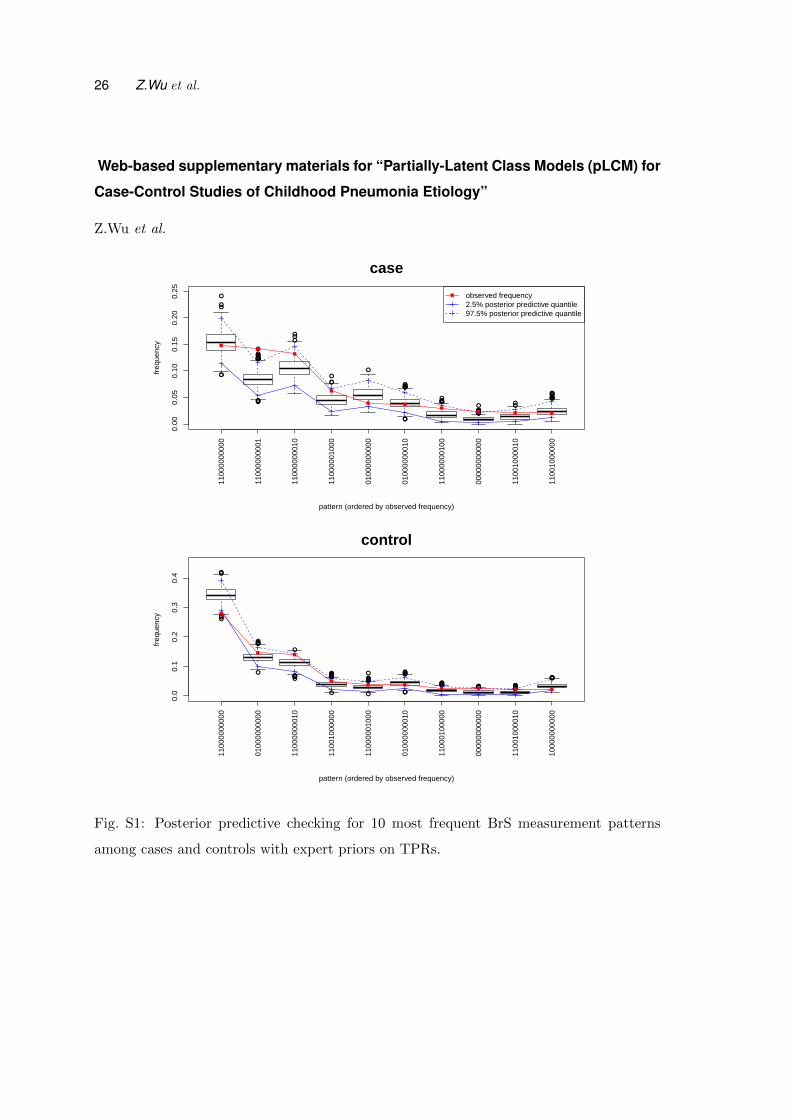
Among the cases, the 95% predictive interval includes the observed values in all but

two of the BrS patterns and even there the fits are reasonable. Among the controls, there

is evidence of lack of fit for the most common BrS pattern with only PNEU and HINF

(Figure S1 in supplementary materials). There are fewer cases with this pattern observed

than predicted under the pLCM. This lack of fit is likely due to associations of pathogen

measurements in control subjects. Note that the FPR estimates remain consistent regard-

less of such correlation as the number of controls increases, however posterior variances

for them may be underestimated.

A second model-checking procedure is for the conditional independence assumption.

We estimated standardized log odds ratios (SLORs) for cases and controls (see Figure

S2 in supplementary materials). Each value is the observed log odds ratio for a pair of

BrS measurements minus the mean LOR from the posterior predictive distribution value,

under the model’s independence assumption, divided by the standard deviation of the

same posterior predictive distribution. We find two large deviations among the cases:

RSV with RHINO and RSV with HMPV. These are likely caused by strong seasonality in

RSV that is out of phase with weaker seasonality in the other two. Otherwise, the number

of SLOR’s greater than 2 (8 out of 110) associations is only slightly larger than what is

expected under the assumed model (6 expected).

An attractive feature of using MCMC to estimate posterior distributions is the ease

of estimating posteriors for functions of the latent variables and/or parameters. One in-

teresting question from a clinical perspective is whether viruses or bacteria are the major

cause and among each subgroup, which species predominate. Figure 4 shows the pos-

terior distribution for the rate of viral pneumonia on the top, and then the conditional

distributions of the two leading viruses (bacteria) among viral (bacterial) causes below on

the right (left). The posterior distribution of the viral etiologic fraction has mode around

70.0% with 95% credible interval (57.0%, 79.2%). As shown at the bottom left in Figure 4,

PNEU accounts for most bacterial cases (47.2% (24.9%, 71.1%)), and SAUR accounts for

25.5% (8.7%, 49.9%). Of all viral cases (bottom right), RSV is estimated to cause about


42.9% (32.8%, 54.8%), and RHINO about 24.2% (13.7%, 37.2%).

5. Discussion

In this paper, we estimated the frequency with which pathogens cause disease in a case

population using a partially-latent class model (pLCM) to allow for known states for

a subset of subjects and for multiple types of measurements with different error rates.

In a case-control study of disease etiology, measurement error will bias estimates from

traditional logistic regression and attributable fraction methods. The pLCM avoids this

pitfall and more naturally incorporates multiple sources of data. Here we formulated the

model with three levels of measurement error rates.

Absent GS data, we show that the pLCM is only partially identified because of the

relationship between the estimated TPR and prevalence of the associated pathogen in the

population. Therefore, the inferences are sensitive to the assumptions about the TPR.

Uncertainty about their values persists in the final inferences from the pLCM regardless

of the number of subjects studied.

The current model provides a novel solution to the analytic problems raised by the

PERCH Study. This paper introduces and applies pLCM to a preliminary set of data

from one PERCH study site. Confirmatory laboratory testing, incorporation of additional

pathogens, and adjustment for potential confounders may change the scientific findings

that will be reported the final complete analysis of the study results when it is completed.

An essential assumption relied upon in the pLCM is that the probability of detecting

one pathogen at a peripheral body site depends on whether that pathogen is infecting

the child’s lung, but is unaffected by the presence of other pathogens in the lung, that is,

the non-differential misclassification error assumption. We have formulated the model to

include GS measures even though they are available only for a small and unrepresentative

subset of the PERCH cases. In general, the availability of GS measures makes it possible

to test this assumption as has been discussed by Albert and Dodd (2008).

Several extensions have potential to improve the quality of inferences drawn and are

being developed for PERCH. First, because the control subjects have known class, we

can model the dependence structure among the BrS measurements and use this to avoid

aspects of the conditional independence assumption central to most LCM methods. The

approach is to extend the pLCM to have K subclasses within each of the current disease

classes. These subclasses can introduce correlation among the BrS measurements given

the true disease state. An interesting question is about the bias-variance trade-off for

18 Z.Wu et al.

different values of K. This ideas follows previous work on the PARAFAC decomposition

of probability distribution for multivariate categorical data (Dunson and Xing, 2009). This

extension will enable model-based checking of the standard pLCM.

Second, in our analyses to date, we have assumed that the pneumonia case definition

is error-free. Given new biomarkers and availability of chest radiographs that can improve

upon the clinical diagnosis of pneumonia, one can introduce an additional latent variable

to indicate true disease status and use these measurements to probabilistically assign each

subject as a case or control. Finally, regression extensions of the pLCM would allow

PERCH investigators to study how the etiology distributions vary with HIV status, age

group, and season.

Acknowledgments

We thank the members of the larger PERCH Study Group for discussions that helped

shape the statistical approach presented herein, and the study participants. We also

thank the members of PERCH Expert Group who provided external advice.

References

Aitchison, J. (1986). The statistical analysis of compositional data. Chapman & Hall, Ltd.

Albert, P. and Dodd, L. (2008). On estimating diagnostic accuracy from studies with

multiple raters and partial gold standard evaluation. Journal of the American Statistical

Association, 103(481):61–73.

Albert, P., McShane, L., and Shih, J. (2001). Latent class modeling approaches for as-

sessing diagnostic error without a gold standard: with applications to p53 immunohis-

tochemical assays in bladder tumors. Biometrics, 57(2):610–619.

Blackwelder, W., Biswas, K., Wu, Y., Kotloff, K., Farag, T., Nasrin, D., Graubard, B.,

Sommerfelt, H., and Levine, M. (2012). Statistical methods in the global enteric multi-

center study (gems). Clinical infectious diseases, 55(suppl 4):S246–S253.

Brooks, S. and Gelman, A. (1998). General methods for monitoring convergence of iterative

simulations. Journal of computational and graphical statistics, 7(4):434–455.

Bruzzi, P., Green, S., Byar, D., Brinton, L., and Schairer, C. (1985). Estimating the

population attributable risk for multiple risk factors using case-control data. American

journal of epidemiology, 122(5):904–914.


Chacon, J., Mateu-Figueras, G., and Martın-Fernandez, J. (2011). Gaussian kernels for

density estimation with compositional data. Computers & Geosciences, 37(5):702–711.

Cutts, F., Zaman, S., Enwere, G. y., Jaffar, S., Levine, O., Okoko, J., Oluwalana, C.,

Vaughan, A., Obaro, S., Leach, A., et al. (2005). Efficacy of nine-valent pneumococcal

conjugate vaccine against pneumonia and invasive pneumococcal disease in the Gambia:

randomised, double-blind, placebo-controlled trial. The Lancet, 365(9465):1139–1146.

Deloria-Knoll, M., Feikin, D., Scott, J., OBrien, K., DeLuca, A., Driscoll, A., Levine, O.,

et al. (2012). Identification and selection of cases and controls in the pneumonia etiology

research for child health project. Clinical Infectious Diseases, 54(suppl 2):S117–S123.

Dunson, D. and Xing, C. (2009). Nonparametric bayes modeling of multivariate categorical

data. Journal of the American Statistical Association, 104(487):1042–1051.

Garrett, E. and Zeger, S. (2000). Latent class model diagnosis. Biometrics, 56(4):1055–

1067.

Goodman, L. (1974). Exploratory latent structure analysis using both identifiable and

unidentifiable models. Biometrika, 61(2):215.

Gustafson, P. (2005). On model expansion, model contraction, identifiability and prior

information: two illustrative scenarios involving mismeasured variables. Statistical Sci-

ence, 20(2):111–140.

Gustafson, P. (2009). What are the limits of posterior distributions arising from noniden-

tified models, and why should we care? Journal of the American Statistical Association,

104(488):1682–1695.

Gustafson, P., Le, N., and Saskin, R. (2001). Case–control analysis with partial knowledge

of exposure misclassification probabilities. Biometrics, 57(2):598–609.

Hui, S. and Walter, S. (1980). Estimating the error rates of diagnostic tests. Biometrics,

36:167–171.

Jones, G., Johnson, W., Hanson, T., and Christensen, R. (2010). Identifiability of models

for multiple diagnostic testing in the absence of a gold standard. Biometrics, 66(3):855–

863.

Kadane, J. (1974). The role of identification in bayesian theory. Studies in Bayesian

Econometrics and Statistics, pages 175–191.

20 Z.Wu et al.

King, G. and Lu, Y. (2008). Verbal autopsy methods with multiple causes of death.

Statistical Science, 23(1):78–91.

Kullback, S. (2012). Information theory and statistics. Courier Dover Publications.

Levine, O., OBrien, K., Deloria-Knoll, M., Murdoch, D., Feikin, D., DeLuca, A., Driscoll,

A., Baggett, H., Brooks, W., Howie, S., et al. (2012). The pneumonia etiology research

for child health project: A 21st century childhood pneumonia etiology study. Clinical

Infectious Diseases, 54(suppl 2):S93–S101.

Madhi, S. A., Kuwanda, L., Cutland, C., and Klugman, K. P. (2005). The impact of a

9-valent pneumococcal conjugate vaccine on the public health burden of pneumonia in

hiv-infected and -uninfected children. Clinical Infectious Diseases, 40(10):1511–1518.

Murdoch, D., OBrien, K., Driscoll, A., Karron, R., Bhat, N., et al. (2012). Laboratory

methods for determining pneumonia etiology in children. Clinical Infectious Diseases,

54(suppl 2):S146–S152.

Qu, Y. and Hadgu, A. (1998). A model for evaluating sensitivity and specificity for

correlated diagnostic tests in efficacy studies with an imperfect reference test. Journal

of the American Statistical Association, 93(443):920–928.

Wang, Z., Zhou, X., and Wang, M. (2011). Evaluation of diagnostic accuracy in detecting

ordered symptom statuses without a gold standard. Biostatistics, 12(3):567–581.


A. Full conditional distributions in Gibbs sampler

In this section, we provide analytic forms of full conditional distributions that are es-

sential for Gibbs sampling algorithm. We use data augmentation scheme by introducing

latent lung state ILi into the sampling chain and we have the following full conditional

distributions:

•[ILi | others

]. If MGS

i is available, Pr(ILi = j | others

)= 1, if MGS

ij = 1 and MGSil =

0, for l 6= j; otherwise zero. If MGSi is missing, according as whether MSS

i is available,

the full conditional is given as

Pr(ILi = j | others) ∝(θBrSj

)MBrSij(1− θBrS

j

)1−MBrSij∏l 6=j

(ψBrSl

)MBrSil(1− ψBrS

l

)1−MBrSil

·[(θSSj

)MSSij (1− θSS

j )1−MSSij 1{∑l6=j M

SSil =0}

]1{j≤J′}

· πj ; (8)

if SS measurement is not available for case i, we remove terms involving MSSij .

•[ψBrSj | others

]∼ Beta

(Nj + b1j , n1 −

∑i:Yi=1 1{ILi =j} + n0 −Nj + b2j

), where n1

and n0 are number of cases and controls, respectively, and Nj =∑

i:Yi=1,ILi 6=jMBrSij +∑

i:Yi=0MBrSij is the number of positives at position j for cases with ILi 6= j and all

controls.

•[θBrSj | others

]∼ Beta

(Sj + c1j ,

∑i:Yi=1 1{ILi =j} − Sj + c2j

), where Sj =

∑i:Yi=1,ILi =jM

BrSij

is the number of positives for cases with jth pathogen as their causes.

•[θSSj | others

]∼ Beta

(Tj + d1j ,

∑i:Yi=1,SS available 1{ILi =j} − Tj + d2j

), where Tj =∑

i:Yi=1,ILi =j,SS availableMSSij . When no SS data is available, this conditional distribu-

tion reduces to Beta(d1j , d2j), the prior.

•[π | ILi , i : Yi = 1

]∼ Dirichlet(a1 + U1, ..., aJ + UJ), where Uj =

∑i:Yi=1 1{ILi =j}.

B. Pathogen names and their abbreviations

Bacteria: HINF- Haemophilus influenzae; PNEU-Streptococcus pneumoniae; SASP-Salmonella

species; SAUR-Staphylococcus aureus. Viruses: ADENO-adenovirus; COR 43-coronavirus

OC43; FLU C-influenza virus type C; HMPV A B-human metapneumovirus type A or B;

PARA1-parainfluenza type 1 virus; RHINO-rhonovirus; RSV A B-respiratory syncytial

virus type A or B.

22 Z.Wu et al.

Fig. 1: Directed acyclic graph (DAG) illustrating relationships among lung infection state

(IL), imperfect lab measurements on the presence/absence of each of a list of pathogens

at each site(MNP , MB and ML), disease outcome (Y ), and covariates (X).


GS=1%

0.8

0.6

0.4

0.2

0.8

0.6

0.4

0.2

0.8

0.6

0.4

0.2

A B

C

95%

●

95%

95% 95%

0.8 0.2

0

(a)

GS=10%

0.8

0.6

0.4

0.2

0.8

0.6

0.4

0.2

0.8

0.6

0.4

0.2

A B

C

95%

● 95% 95%

95%

0.62 0.28

0.1

(b)

GS=1%

0.8

0.6

0.4

0.2

0.8

0.6

0.4

0.2

0.8

0.6

0.4

0.2

A B

C

000

001

010

011

100

101

110

111

0.8 0.2

0

(c)

GS=10%

0.8

0.6

0.4

0.2

0.8

0.6

0.4

0.2

0.8

0.6

0.4

0.2

A B

C

000

001

010

011

100

101

110

111

0.62 0.28

0.1

(d)

Fig. 2: Population (top) and individual (bottom) etiology estimations for a single sample

with 500 cases and 500 controls with true π = (0.67, 0.26, 0.07)′ and either 1%(N = 5) or

10%(N = 50) GS data on cases. In (a) or (b), red circled plus shows the true population

etiology distribution π. The closed curves are 95% credible regions for analysis using

BrS data only (blue dashed lines “- - -”), BrS+GS data (light green solid lines “—”), GS

data only (textitblack dotted lines “· · · ”); Solid square/dot/triangle are the corresponding

posterior means of π; The 95% highest density region of uniform prior distribution is

also visualized by red “· − ·−” for comparison. In (c) or (d), 8(= 23) BrS measurement

patterns and predictions for individual children are shown with measurement patterns

attached. The numbers at the vertices show empirical frequencies of GS measurements.

24 Z.Wu et al.

●

●

●

●

●

●

●

●

●

●

●

●

●

●

●

●

●

●

●

●

●

●

probability

case

ctrl

case

ctrl

case

ctrl

case

ctrl

case

ctrl

case

ctrl

case

ctrl

case

ctrl

case

ctrl

case

ctrl

case

ctrl

0 0.2 0.4 0.6 0.8 1

+|

|

+|

|

+|

|

+|

|

+|

|

+|

|

+|

|

+|

|

+|

|

+|

|

+|

|

*|

|

*|

|

*|

|

*|

|

*|

|

*|

|

*|

|

*|

|

*|

|

*|

|

*|

|

0.40.1 1.7

0.90.5 1.7

0.30 2

1.20.7 1.8

1.30.9 1.8

5.92.6 15.1

10.6 1.7

2.51.6 3.9

0.70.4 1.1

1.51.1 2.1

52.921.7 175

conditional OR

0.7%

1.7%

4.6%

5.6%

0.2%

1%

10%

11.1%

75.9%

69.9%

5.6%

1.5%

7.9%

8.4%

14.6%

9.2%

88.6%

91%

29.2%

29%

25.1%

0.8%

BrS

●

●

●

●

●

●

●

●

0.0 0.2 0.4 0.6 0.8 1.0

probability

|

|

|

|

|

|

|

|

|

|

|

|

|

|

|

|

[

|

[

|

[

|

[

|

]

|

]

|

]

|

]

|

0.5%

1.6%

0.2%

0.9%

9.13 %

| |[ ]

10.11 %

| |[ ]

9.5 %

| |[ ]

9.97 %

| |[ ]

SS

●

●

●

●

●

●

●

●

●

●

●

0.0 0.1 0.2 0.3 0.4 0.5

probability

FLU_C

COR_43

SASP

ADENO

HINF

PARA1

SAUR

HMPV_A_B

PNEU

RHINO

RSV_A_B

0.0 0.2 0.4

0.0 0.2 0.4

0.0 0.2 0.4

0.0 0.2 0.4

0.0 0.2 0.4

0.0 0.2 0.4

0.0 0.2 0.4

0.0 0.2 0.4

0.0 0.2 0.4

0.0 0.2 0.4

|

|

|

|

|

|

|

|

|

|

|

|

|

|

|

|

|

|

|

|

|

|

[

[

[

[

[

[

[

[

[

[

[

]

]

]

]

]

]

]

]

]

]

]

πprior posterior

=0.6%π7

=1.1%π6

=2.6%π3

=3.2%π5

=5.9%π1

=6.4%π9

=8%π4

=11.4%π8

=14.8%π2

=16.7%π10

=29.4%π11

Fig. 3: The observed BrS rates (with 95% confidence intervals) for cases and controls are

shown on the far left. The conditional odds ratio given the other pathogens is listed with

95% confidence interval in the box to the right of the BrS data summary. In the left box,

below the case and control observed rates is a horizontal line with a triangle. The line

starts on the left at the model estimated false positive rate (FPR, ψBrSj ) and ends on the

right at the estimated true positive rate (TPR, θBrSj ). Below the TPR are two boxplots

summarizing its posterior (top) and prior (bottom) distributions. The location of the

triangle, expressed as a fraction of the distance from the estimated FPR to the TPR, is

the point estimate of the etiologic fraction for each pathogen. The SS data are shown in a

similar fashion to the right of the BrS data using support intervals rather than boxplots.


0.0 0.2 0.4 0.6 0.8 1.0

Probability of Viral Cause

0.8

0.6

0.4

0.2

0.8

0.6

0.4

0.2

0.8

0.6

0.4

0.2

95%

B−rest SAUR

PNEU

0.8

0.6

0.4

0.2

0.8

0.6

0.4

0.2

0.8

0.6

0.4

0.2

95%

RHINO V−rest

RSV_A_B

Fig. 4: Summary of posterior distribution of pneumonia etiology estimates. Top: posterior

distribution of viral etiology; bottom left (right): posterior etiology distribution for top

two causes given a bacterial (viral) infection. The blue circles are the 95% credible regions

within the bacterial or viral groups.

26 Z.Wu et al.

Web-based supplementary materials for “Partially-Latent Class Models (pLCM) for

Case-Control Studies of Childhood Pneumonia Etiology”

Z.Wu et al.

●

●

●

●

●

●

●

●●

●●

●

●

●●●●●●●●

●●●

●●

●

●

●

●●●●●●

●

●●●

●●●●●●

●●●●●●●●●●●●●●●●●●●●●●●●●●●●●●●●●●●●●

●

●●●

●●

●●●●●●●●●●●

0.00

0.05

0.10

0.15

0.20

0.25

case

freq

uenc

y

pattern (ordered by observed frequency)

1100

0000

000

1100

0000

001

1100

0000

010

1100

0001

000

0100

0000

000

0100

0000

010

1100

0000

100

0000

0000

000

1100

1000

010

1100

1000

000

observed frequency2.5% posterior predictive quantile97.5% posterior predictive quantile

●●●

●●

●●

●

●●●

●●●●●●

●

●●●●●

●

●●●●●●●●●

●●

●

●

●

●●●●●●●●●●●●●●●●●

●●

●●

●●●

●●●●●●●●● ●●●●●● ●●●●●●●●●●●●●●●●●●●●●●●●●●●●●●●

●●●●●

0.0

0.1

0.2

0.3

0.4

control

freq

uenc

y

pattern (ordered by observed frequency)

1100

0000

000

0100

0000

000

1100

0000

010

1100

1000

000

1100

0001

000

0100

0000

010

1100

0100

000

0000

0000

000

1100

1000

010

1000

0000

000

Fig. S1: Posterior predictive checking for 10 most frequent BrS measurement patterns

among cases and controls with expert priors on TPRs.


HIN

F

PN

EU

SA

SP

SA

UR

AD

EN

OV

IRU

S

CO

R_4

3

FLU

_C

HM

PV

_A_B

PAR

A1

RH

INO

RS

V_A

_BRSV_A_B

RHINO

PARA1

HMPV_A_B

FLU_C

COR_43

ADENOVIRUS

SAUR

SASP

PNEU

HINF

−2.3

4

−2.1

2.2

2.1

−5.2

−2.5

−4.2

case

control

Fig. S2: Posterior predictive checking for pairwise odds ratios separately for cases (lower

triangle) and controls (upper triangle) with expert priors on TPRs. Each entry is a

standardized log odds ratio (SLOR): the observed log odds ratio for a pair of BrS mea-

surements minus the mean LOR for the posterior predictive distribution divided by the

standard deviation of the posterior predictive distribution. The first significant digit of

absolute SLORs are shown in red for positive and blue for negative values, and only those

greater than 2 are shown.

Partially-Latent Class Models (pLCM) for Case-Control ... · Partially-Latent Class Models (pLCM) for Case-Control Studies of Childhood Pneumonia Etiology ... analysis of the motivating

Documents