Journal of Machine Learning Research 22 (2021) 1-46 Submitted 5/20; Revised 3/21; Published 10/21 Partial Policy Iteration for L 1 -Robust Markov Decision Processes Chin Pang Ho [email protected] School of Data Science City University of Hong Kong 83 Tat Chee Avenue Kowloon Tong, Hong Kong Marek Petrik [email protected] Department of Computer Science University of New Hampshire Durham, NH, USA, 03861 Wolfram Wiesemann [email protected] Imperial College Business School Imperial College London London SW7 2AZ, United Kingdom Editor: Ambuj Tewari Abstract Robust Markov decision processes (MDPs) compute reliable solutions for dynamic deci- sion problems with partially-known transition probabilities. Unfortunately, accounting for uncertainty in the transition probabilities significantly increases the computational com- plexity of solving robust MDPs, which limits their scalability. This paper describes new, efficient algorithms for solving the common class of robust MDPs with s- and sa-rectangular ambiguity sets defined by weighted L 1 norms. We propose partial policy iteration, a new, efficient, flexible, and general policy iteration scheme for robust MDPs. We also propose fast methods for computing the robust Bellman operator in quasi-linear time, nearly match- ing the ordinary Bellman operator’s linear complexity. Our experimental results indicate that the proposed methods are many orders of magnitude faster than the state-of-the-art approach, which uses linear programming solvers combined with a robust value iteration. Keywords: Robust Markov decision processes, optimization, reinforcement learning 1. Introduction Markov decision processes (MDPs) provide a versatile methodology for modeling and solving dynamic decision problems under uncertainty (Puterman, 2005). Unfortunately, however, MDP solutions can be very sensitive to estimation errors in the transition probabilities and rewards. This is of particular worry in reinforcement learning applications, where the model is fit to data and therefore inherently uncertain. Robust MDPs (RMDPs) do not assume that the transition probabilities are known precisely but instead allow them to take on any value from a given ambiguity set or uncertainty set (Xu and Mannor, 2006; Mannor et al., 2012; Hanasusanto and Kuhn, 2013; Tamar et al., 2014; Delgado et al., 2016). With c 2021 Chin Pang Ho, Marek Petrik, and Wolfram Wiesemann. License: CC-BY 4.0, see https://creativecommons.org/licenses/by/4.0/. Attribution requirements are provided at http://jmlr.org/papers/v22/20-445.html.

Welcome message from author
This document is posted to help you gain knowledge. Please leave a comment to let me know what you think about it! Share it to your friends and learn new things together.
Transcript

Journal of Machine Learning Research 22 (2021) 1-46 Submitted 5/20; Revised 3/21; Published 10/21
Partial Policy Iterationfor L1-Robust Markov Decision Processes
Chin Pang Ho [email protected] of Data ScienceCity University of Hong Kong83 Tat Chee AvenueKowloon Tong, Hong Kong
Marek Petrik [email protected] of Computer ScienceUniversity of New HampshireDurham, NH, USA, 03861
Wolfram Wiesemann [email protected]
Imperial College Business School
Imperial College London
London SW7 2AZ, United Kingdom
Editor: Ambuj Tewari
Abstract
Robust Markov decision processes (MDPs) compute reliable solutions for dynamic deci-sion problems with partially-known transition probabilities. Unfortunately, accounting foruncertainty in the transition probabilities significantly increases the computational com-plexity of solving robust MDPs, which limits their scalability. This paper describes new,efficient algorithms for solving the common class of robust MDPs with s- and sa-rectangularambiguity sets defined by weighted L1 norms. We propose partial policy iteration, a new,efficient, flexible, and general policy iteration scheme for robust MDPs. We also proposefast methods for computing the robust Bellman operator in quasi-linear time, nearly match-ing the ordinary Bellman operator’s linear complexity. Our experimental results indicatethat the proposed methods are many orders of magnitude faster than the state-of-the-artapproach, which uses linear programming solvers combined with a robust value iteration.
Keywords: Robust Markov decision processes, optimization, reinforcement learning
1. Introduction
Markov decision processes (MDPs) provide a versatile methodology for modeling and solvingdynamic decision problems under uncertainty (Puterman, 2005). Unfortunately, however,MDP solutions can be very sensitive to estimation errors in the transition probabilitiesand rewards. This is of particular worry in reinforcement learning applications, where themodel is fit to data and therefore inherently uncertain. Robust MDPs (RMDPs) do notassume that the transition probabilities are known precisely but instead allow them to takeon any value from a given ambiguity set or uncertainty set (Xu and Mannor, 2006; Mannoret al., 2012; Hanasusanto and Kuhn, 2013; Tamar et al., 2014; Delgado et al., 2016). With
c©2021 Chin Pang Ho, Marek Petrik, and Wolfram Wiesemann.
License: CC-BY 4.0, see https://creativecommons.org/licenses/by/4.0/. Attribution requirements are providedat http://jmlr.org/papers/v22/20-445.html.

Ho, Petrik, and Wiesemann
appropriately chosen ambiguity sets, RMDP solutions are often much less sensitive to modelerrors (Xu and Mannor, 2009; Petrik, 2012; Petrik et al., 2016).
Most of the RMDP literature assumes rectangular ambiguity sets that constrain theerrors in the transition probabilities independently for each state (Iyengar, 2005; Nilim andEl Ghaoui, 2005; Le Tallec, 2007; Kaufman and Schaefer, 2013; Wiesemann et al., 2013).This assumption is crucial to retain many of the desired structural features of MDPs. Inparticular, the robust return of an RMDP with a rectangular ambiguity set is maximized bya stationary policy, and the optimal value function satisfies a robust variant of the Bellmanoptimality equation. Rectangularity also ensures that an optimal policy can be computedin polynomial time by robust versions of the classical value or policy iteration (Iyengar,2005; Hansen et al., 2013).
A particularly popular class of rectangular ambiguity sets is defined by bounding theL1-distance of any plausible transition probabilities from a nominal distribution (Iyengar,2005; Strehl et al., 2009; Jaksch et al., 2010; Petrik and Subramanian, 2014; Taleghanet al., 2015; Petrik et al., 2016). Such ambiguity sets can be readily constructed fromsamples (Weissman et al., 2003; Behzadian et al., 2021), and their polyhedral structureimplies that the worst transition probabilities can be computed by the solution of linearprograms (LPs). Unfortunately, even for the specific class of L1-ambiguity sets, an LPhas to be solved for each state and each step of the value or policy iteration. Generic LPalgorithms have a worst-case complexity that is approximately quartic in the number ofstates (Vanderbei, 1998), and they thus become prohibitively expensive for large RMDPs.
In this paper, we propose a new framework for solving RMDPs. Our framework ap-plies to both sa-rectangular ambiguity sets, where adversarial nature observes the agent’sactions before choosing the worst plausible transition probabilities (Iyengar, 2005; Nilimand El Ghaoui, 2005), and s-rectangular ambiguity sets, where nature must commit to arealization of the transition probabilities before observing the agent’s actions (Le Tallec,2007; Wiesemann et al., 2013). We achieve a significant theoretical and practical accelera-tion over the robust value and policy iteration by reducing the number of iterations neededand by reducing the computational complexity of each iteration. The overall speedup of ourframework—both theoretical and practical—allows us to solve RMDPs with L1-ambiguitysets in a time complexity that is similar to that of classical MDPs. Our framework comprisesof three components, each of which represents a novel contribution.
Our first contribution is partial policy iteration (PPI), which generalizes the classi-cal modified policy iteration to RMDPs. PPI resembles the robust modified policy itera-tion (Kaufman and Schaefer, 2013), which has been proposed for sa-rectangular ambiguitysets. In contrast to the robust modified policy iteration, however, PPI applies to both sa-rectangular and s-rectangular ambiguity sets, and it is guaranteed to converge at the samelinear rate as robust value and robust policy iteration. In our experimental results, PPIoutperforms robust value iteration by several orders of magnitude.
Our second contribution is a fast algorithm for computing the robust Bellman opera-tor for sa-rectangular weighted L1-ambiguity sets. Our algorithm employs the homotopycontinuation strategy (Vanderbei, 1998): it starts with a singleton ambiguity set for whichthe worst transition probabilities can be trivially identified, and it subsequently traces themost adverse transition probabilities as the size of the ambiguity set increases. The time
2
Partial Policy Iteration for Robust MDPs
complexity of our homotopy method is quasi-linear in the number of states and actions,which is significantly faster than the quartic worst-case complexity of generic LP solvers.
Our third contribution is a fast algorithm for computing the robust Bellman operatorfor s-rectangular weighted L1-ambiguity sets. While often less conservative and hence moreappropriate in practice, s-rectangular ambiguity sets are computationally challenging sincethe agent’s optimal policy can be randomized (Wiesemann et al., 2013). We propose abisection approach to decompose the s-rectangular Bellman computation into a series ofsa-rectangular Bellman computations. When our bisection method is combined with ourhomotopy method, its time complexity is quasi-linear in the number of states and actions,compared again to the quartic complexity of generic LP solvers.
Put together, our contributions comprise a complete framework that can be used tosolve RMDPs efficiently. Besides being faster than solving LPs directly, our frameworkdoes not require an expensive black-box commercial optimization package such as CPLEX,Gurobi, or Mosek. A well-tested and documented implementation of the methods describedin this paper is available at https://github.com/marekpetrik/craam2. Compared to anearlier conference version of this work (Ho et al., 2018), the present paper introduces PPI, itimproves the bisection method to work with PPI, it provides extensive and simpler proofs,and it reports more complete experimental results.
The remainder of the paper is organized as follows. We summarize relevant prior workin Section 2 and subsequently review basic properties of RMDPs in Section 3. Section 4describes our partial policy iteration (PPI), Section 5 develops the homotopy method forsa-rectangular ambiguity sets, and Section 6 is devoted to the bisection method for s-rectangular ambiguity sets. Section 7 compares our algorithms with the solution of RMDPsvia Gurobi, a leading commercial LP solver, and we offer concluding remarks in Section 8.
We use the following notation throughout the paper. Regular lowercase letters (suchas p) denote scalars, boldface lowercase letters (such as p) denote vectors, and boldfaceuppercase letters (such as X) denote matrices. Indexed values are printed in bold if theyare vectors and in regular font if they are scalars. That is, pi refers to the i-th componentof a vector p, whereas pi is the i-th vector of a sequence of vectors. An expression inparentheses indexed by a set of natural numbers, such as ppiqiPZ for Z “ t1, . . . , ku, denotesthe vector pp1, p2, . . . , pkq. Similarly, if each pi is a vector, then P “ ppiqiPZ is a matrix witheach vector pJi as a row. The expression ppiqj P R represents the component in i-th row andj-th column. All vector inequalities are understood to hold component-wise. Calligraphicletters and uppercase Greek letters (such as X and Ξ) are reserved for sets. The symbols 1and 0 denote vectors of all ones and all zeros, respectively, of the size appropriate to theircontext. The symbol I denotes the identity matrix of the appropriate size. The probabilitysimplex in RS` is denoted as ∆S “
p P RS` | 1Jp “ 1(
. The set R represents real numbersand the set R` represents non-negative real numbers.
2. Related Work
We review relevant prior work that aims at (i) reducing the number of iterations needed tocompute an optimal RMDP policy, as well as (ii) reducing the computational complexityof each iteration. We also survey algorithms for related machine learning problems.
3

Ho, Petrik, and Wiesemann
The standard approach for computing an optimal RMDP policy is robust value iteration,which is a variant of the classical value iteration for ordinary MDPs that iteratively appliesthe robust Bellman operator to an increasingly accurate approximation of the optimal robustvalue function (Givan et al., 2000; Iyengar, 2005; Le Tallec, 2007; Wiesemann et al., 2013).Robust value iteration is easy to implement and versatile, and it converges linearly with arate of γ, the discount factor of the RMDP.
Unfortunately, robust value iteration requires many iterations and thus performs poorlywhen the discount factor of the RMDP approaches 1. To alleviate this issue, robust policyiteration alternates between robust policy evaluation steps that determine the robust valuefunction for a fixed policy and policy improvement steps that select the optimal greedypolicy for the current estimate of the robust value function (Iyengar, 2005; Hansen et al.,2013). While the theoretical convergence rate guarantee for robust policy iteration matchesthat for robust value iteration, its practical performance tends to be superior for discountfactors close to 1. However, unlike the classical policy iteration for ordinary MDPs, whichsolves a system of linear equations in each policy evaluation step, robust policy iterationsolves a large LP in each robust policy evaluation step. The need to solve large LPs restrictsrobust policy iteration to small RMDPs.
Modified policy iteration, also known as optimistic policy iteration, tends to significantlyoutperform both value and policy iteration on ordinary MDPs (Puterman, 2005). Modifiedpolicy iteration adopts the same strategy as policy iteration, but it merely approximates thevalue function in each policy evaluation step by executing a small number of value iterations.Generalizing the modified policy iteration to RMDPs is not straightforward. There wereseveral early attempts to develop a robust modified policy iteration (Satia and Lave, 1973;White and Eldeib, 1994), but their convergence guarantees are in doubt (Kaufman andSchaefer, 2013). The challenge is that the alternating maximization (in the policy improve-ment step) and minimization (in the policy evaluation step) may lead to infinite cycles inthe presence of approximation errors. Several natural robust policy iteration variants havebeen shown to loop infinitely on some inputs (Condon, 1993).
To the best of our knowledge, robust modified policy iteration (RMPI) is the first gen-eralization of the classical modified policy iteration to RMDPs with provable convergenceguarantees (Kaufman and Schaefer, 2013). RMPI alternates between robust policy evalua-tion steps and policy improvement steps. The robust policy evaluation steps approximatethe robust value function of a fixed policy by executing a small number of value iterations,and the policy improvement steps select the optimal greedy policy for the current esti-mate of the robust value function. Our partial policy iteration (PPI) improves on RMPIin several respects. RMPI only applies to sa-rectangular problems in which there existoptimal deterministic policies, while PPI also applies to s-rectangular problems in whichall optimal policies may be randomized. Also, RMPI relies on value iteration to partiallyevaluate a fixed policy, whereas PPI can evaluate the fixed policy more efficiently usingother schemes such as policy or modified policy iteration. Finally, PPI enjoys a guaranteedlinear convergence rate of γ, the discount factor of the RMDP.
Besides value and (modified) policy iteration, ordinary MDPs have been successfullysolved with accelerated value iteration, which reduces the number of required Bellmanoperator evaluations. Recent accelerated value iteration methods have employed Andersonand Nesterov-type acceleration approaches (Geist and Scherrer, 2018; Goyal and Grand-
4

Partial Policy Iteration for Robust MDPs
Clement, 2019; Zhang et al., 2020). These acceleration schemes eschew policy evaluationin lieu of computing a linear combination of recent value function iterates. However, it isunclear how these accelerated value iteration approaches can be generalized to RMDPs.
In addition to accelerating value iteration, prior work has also focused on speeding upthe computation of the robust Bellman operator for structured ambiguity sets. While thisevaluation amounts to the solution of a convex optimization problem for generic convexambiguity sets and reduces to the solution of an LP for polyhedral ambiguity sets, theresulting polynomial runtime guarantees are insufficient due to the large number of evalu-ations required. Quasi-linear time algorithms for computing Bellman updates for RMDPswith unweighted sa-rectangular L1-ambiguity sets have been proposed by Iyengar (2005)and Petrik and Subramanian (2014). Similar algorithms have been used to guide the explo-ration of MDPs (Strehl et al., 2009; Taleghan et al., 2015). In contrast, our algorithm forsa-rectangular ambiguity sets applies to both unweighted and weighted L1-ambiguity sets,where the latter ones have been shown to provide superior robustness guarantees (Behza-dian et al., 2021). The extension to weighted norms requires a surprisingly large change tothe algorithm. Quasi-linear time algorithms have also been proposed for sa-rectangular L8-ambiguity sets (Givan et al., 2000), L2-ambiguity sets (Iyengar, 2005), and KL-ambiguitysets (Iyengar, 2005; Nilim and El Ghaoui, 2005). We are not aware of any previous special-ized algorithms for s-rectangular ambiguity sets, which are significantly more challengingas all optimal policies may be randomized, and it is therefore not possible to compute theworst transition probabilities independently for each action.
Our algorithm for computing the robust Bellman operator over an sa-rectangular ambi-guity set resembles LARS, a homotopy method for solving the LASSO problem (Drori andDonoho, 2006; Hastie et al., 2009; Murphy, 2012). It also resembles methods for computingfast projections onto the L1-ball (Duchi et al., 2008; Thai et al., 2015) and the weightedL1-ball (van den Berg and Friedlander, 2011). In contrast to those works, our algorithmoptimizes a linear function (instead of a more general quadratic one) over the intersectionof the (weighted) L1-ball and the probability simplex (as opposed to the entire L1-ball).
Our algorithm for computing the robust Bellman operator for s-rectangular ambiguitysets employs a bisection method. This is a common optimization technique for solving low-dimensional problems. We are not aware of works that use bisection to solve s-rectangularRMDPs or similar machine learning problems. However, a bisection method has beenpreviously used to solve sa-rectangular RMDPs with KL-ambiguity sets (Nilim and ElGhaoui, 2005). That bisection method, however, has a different motivation, solves a differentproblem, and bisects on different problem parameters.
Throughout this paper, we focus on RMDPs with sa-rectangular or s-rectangular ambi-guity sets but note that several more-general classes have been proposed recently (Mannoret al., 2012, 2016; Goyal and Grand-Clement, 2018). These k-rectangular and r-rectangularsets have tangible advantages, but also introduce additional computational complications.
3. Robust Markov Decision Processes
This section surveys RMDPs and their basic properties. We cover both sa-rectangular ands-rectangular ambiguity sets but limit the discussion to norm-constrained ambiguity sets.
5

Ho, Petrik, and Wiesemann
An MDP pS,A,p0,p, r, γq is described by a state set S “ t1, . . . , Su and an actionset A “ t1, . . . , Au. The initial state is selected randomly according to the distributionp0 P ∆S . When the MDP is in state s P S, taking the action a P A results in a stochastictransition to a new state s1 P S according to the distribution ps,a P ∆S with a reward ofrs,a,s1 P R. We condense the transition probabilities ps,a to the transition function p “pps,aqsPS,aPA P p∆
SqSˆA which can also be also interpreted as a function p : S ˆA Ñ ∆S .Similarly, we condense the rewards to vectors rs,a “ prs,a,s1qs1PS P RS and r “ prs,aqsPS,aPA.The discount factor is γ P p0, 1q.
A (stationary) randomized policy π “ pπsqsPS , πs P ∆A for all s P S, is a function thatprescribes to take an action a P A with the probability πs,a whenever the MDP is in a states P S. We use Π “ p∆AqS to denote the set of all randomized stationary policies.
For a given policy π P Π, an MDP becomes a Markov reward process, which is aMarkov chain with the SˆS transition matrix P pπq “ ppspπqqsPS and the rewards rpπq “prspπqqsPS P RS where
pspπq “ÿ
aPAπs,a ¨ ps,a and rspπq “
ÿ
aPAπs,a ¨ p
Js,ars,a ,
and pspπq P ∆S and rspπq P R. The total expected discounted reward of this Markovreward process is
E
«
8ÿ
t“0
γt ¨ rSt,At,St`1
ff
“ pJ0 pI ´ γ ¨ P pπqq´1rpπq .
Here, the initial random state S0 is distributed according to p0, the subsequent randomstates S1, S2, . . . are distributed according to ppπq, and the random actions A0, A1, . . . aredistributed according to π. The value function of this Markov reward process is vpπ,pq “pI´γ ¨P pπqq´1rpπq. For each state s P S, vspπ,pq describes the total expected discountedreward once the Markov reward process enters s. It is well-known that the total expecteddiscounted reward of an MDP is optimized by a deterministic policy π satisfying πs,a P t0, 1ufor each s P S and a P A (Puterman, 2005).
RMDPs generalize MDPs in that they account for the uncertainty in the transitionfunction p. More specifically, the RMDP pS,A,p0,P, r, γq assumes that the transitionfunction p is chosen adversarially from an ambiguity set (or uncertainty set) of plausiblevalues P Ď p∆SqSˆA (Hanasusanto and Kuhn, 2013; Wiesemann et al., 2013; Petrik andSubramanian, 2014; Petrik et al., 2016; Russell and Petrik, 2019). The objective is tocompute a policy π P Π that maximizes the return, or the expected sum of discountedrewards, under the worst-case transition function from P:
maxπPΠ
minpPP
pJ0 vpπ,pq . (3.1)
The maximization in (3.1) represents the objective of the agent, while the minimization canbe interpreted as the objective of adversarial nature. To ensure that the minimum exists,we assume throughout the paper that the set P is compact.
The optimal policies in RMDPs are history-dependent, stochastic and NP-hard to com-pute even when restricted to be stationary (Iyengar, 2005; Wiesemann et al., 2013). How-ever, the problem (3.1) is tractable for some broad classes of ambiguity sets P. The most
6

Partial Policy Iteration for Robust MDPs
common such class are the sa-rectangular ambiguity sets, which are defined as Cartesianproducts of sets Ps,a Ď ∆S for each state s and action a (Iyengar, 2005; Nilim and ElGhaoui, 2005; Le Tallec, 2007):
P “!
p P p∆SqSˆA | ps,a P Ps,a @s P S, a P A)
. (3.2)
Since each probability vector ps,a belongs to a separate set Ps,a, adversarial nature can selectthe worst transition probabilities independently for each state and action. This amounts tonature being able to observe the agent’s action prior to choosing the transition probabilities.Similar to ordinary MDPs, there always exists an optimal deterministic stationary policyin sa-rectangular RMDPs (Iyengar, 2005; Nilim and El Ghaoui, 2005).
In this paper, we study sa-rectangular ambiguity sets that constitute weighted L1-ballsaround some nominal transition probabilities ps,a P ∆S :
Ps,a “
p P ∆S | }p´ ps,a}1,ws,a ď κs,a(
Here, the weights ws,a P RS` are assumed to be strictly positive: ws,a ą 0, s P S, a P A. Theradius κs,a P R` of the ball is called the budget, and the weighted L1-norm is defined as
}x}1,w “nÿ
i“1
wi |xi| .
The weights ws,a can be used to control the shape of the ambiguity sets to compute betterpolicies. For example, RMDPs with optimized weights ws,a provide significantly improvedpercentile criterion guarantees compared to uniform weights (Behzadian et al., 2021).
L1-ball ambiguity sets have gained popularity in RMDPs (Iyengar, 2005; Petrik andSubramanian, 2014; Petrik et al., 2016; Derman et al., 2019; Behzadian et al., 2021) andoptimistic MDPs (Strehl et al., 2009; Jaksch et al., 2010; Taleghan et al., 2015) for thefollowing reasons. First, the L1-distance between probability distributions corresponds tothe total variation distance, a simple and intuitive statistical distance metric. Second,the robust Bellman operator over the L1-ambiguity set can be solved as a linear programusing mature, widely-available solvers. And third, RMDPs combined with existing L1-normconcentration inequalities can be used to provide finite sample guarantees (Weissman et al.,2003; Petrik et al., 2016; Behzadian et al., 2021).
Similarly to MDPs, the robust value function vπ “ minpPP vpπ,pq of an sa-rectangularRMDP for a policy π P Π can be computed using the robust Bellman policy update Lπ :RS Ñ RS . For sa-rectangular RMDPs constrained by the L1-norm, the operator Lπ isdefined for each state s P S as
pLπvqs “ÿ
aPA
ˆ
πs,a ¨ minpPPs,a
pJprs,a ` γ ¨ vq
˙
“ÿ
aPA
ˆ
πs,a ¨ minpP∆S
pJprs,a ` γ ¨ vq | }p´ ps,a}1,ws,a ď κs,a(
˙
.
(3.3)
The robust value function is the unique solution to vπ “ Lπvπ (Iyengar, 2005). To computethe optimal value function, we use the sa-rectangular robust Bellman optimality operator
7
Ho, Petrik, and Wiesemann
L : RS Ñ RS defined as
pLvqs “ maxaPA
minpPPs,a
pJprs,a ` γ ¨ vq
“ maxaPA
minpP∆S
pJprs,a ` γ ¨ vq | }p´ ps,a}1,ws,a ď κs,a(
.(3.4)
Let π‹ P Π be an optimal robust policy which solves (3.1). Then the optimal robust valuefunction v‹ “ vπ‹ is the unique vector that satisfies v‹ “ Lv‹ (Iyengar, 2005; Wiesemannet al., 2013). In addition, a policy π is called greedy for a value function v wheneverLπv “ Lv.
The value p P ∆S in the equations above represents a probability vector rather than thetransition function p P p∆SqSˆA. To prevent confusion between the two in the remainderof the paper, we specify the dimensions of p whenever it is not obvious from its context.
As mentioned above, sa-rectangular sets assume that nature can observe the agent’saction when choosing the robust transition probabilities. This assumption grants naturetoo much power and often results in overly conservative policies (Le Tallec, 2007; Wiesemannet al., 2013). S-rectangular ambiguity sets partially alleviate this issue while preserving thecomputational tractability of sa-rectangular sets. They are defined as Cartesian productsof sets Ps Ď p∆SqA for each state s (as opposed to state-action pairs earlier):
P “
p P p∆SqSˆA | pps,aqaPA P Ps @s P S(
(3.5)
Since the probability vectors ps,a, a P A, for the same state s are subjected to the jointconstraints captured by Ps, adversarial nature can no longer select the worst transition prob-abilities independently for each state and action. The presence of these joint constraintsamounts to nature choosing the transition probabilities while only observing the state andnot the agent’s action (but observing the agent’s policy). In contrast to ordinary MDPsand sa-rectangular RMDPs, s-rectangular RMDPs are optimized by randomized policiesin general (Le Tallec, 2007; Wiesemann et al., 2013). As before, we restrict our atten-tion to s-rectangular ambiguity sets defined in terms of L1-balls around nominal transitionprobabilities:
Ps “
#
p P p∆SqA |ÿ
aPA‖pa ´ ps,a‖1,ws,a ď κs
+
In contrast to the earlier sa-rectangular ambiguity set, nature is now restricted by a singlebudget κs P R` for all transition probabilities pps,aqaPA relating to a state s P S. We notethat although sa-rectangular ambiguity sets are a special case of s-rectangular ambiguitysets in general (Wiesemann et al., 2013), this is not true for our particular classes of L1-ballambiguity sets.
The s-rectangular robust Bellman policy update Lπ : RS Ñ RS is defined as
pLπvqs “ minpPPs
ÿ
aPA
`
πs,a ¨ pJa prs,a ` γ ¨ vq
˘
“ minpPp∆SqA
#
ÿ
aPAπs,a ¨ p
Ja prs,a ` γ ¨ vq |
ÿ
aPA‖pa ´ ps,a‖1,ws,a ď κs
+
.
(3.6)
8
Partial Policy Iteration for Robust MDPs
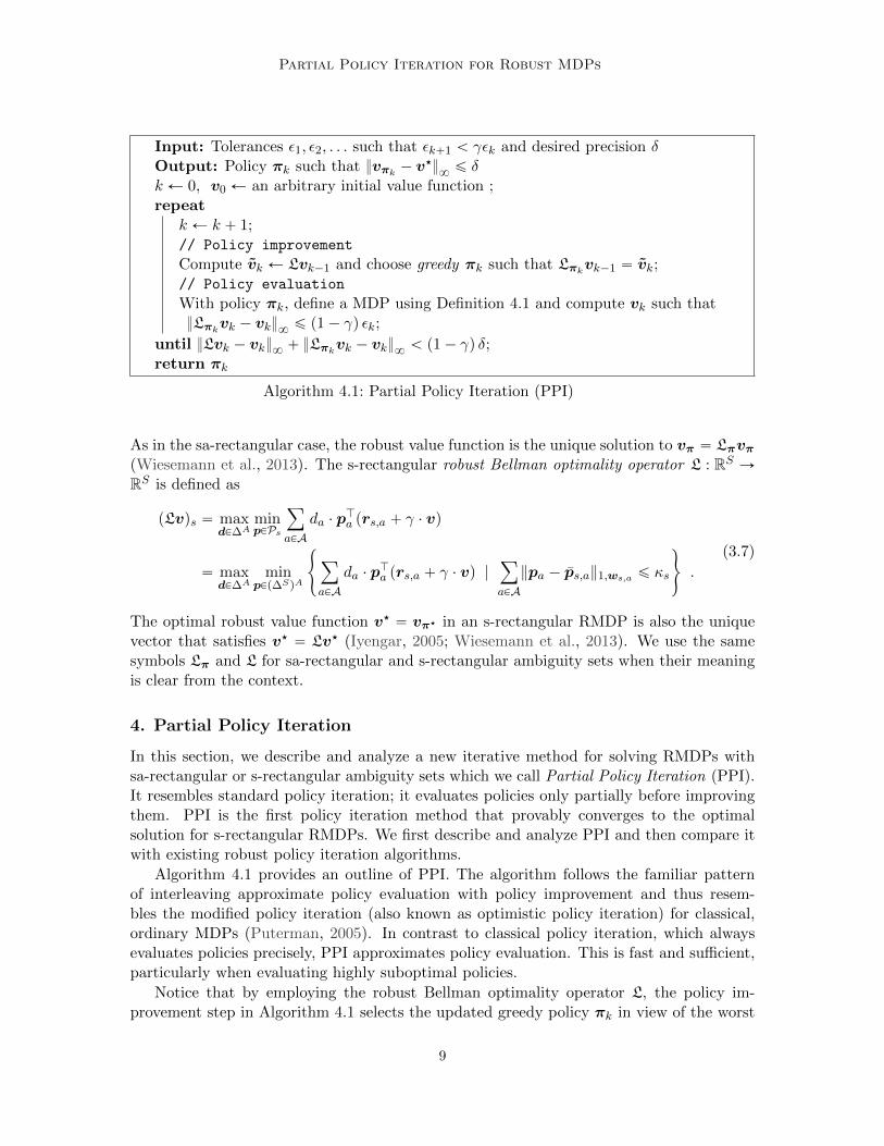
Input: Tolerances ε1, ε2, . . . such that εk`1 ă γεk and desired precision δOutput: Policy πk such that }vπk
´ v‹}8ď δ
k Ð 0, v0 Ð an arbitrary initial value function ;repeat
k Ð k ` 1;// Policy improvement
Compute vk Ð Lvk´1 and choose greedy πk such that Lπkvk´1 “ vk;
// Policy evaluation
With policy πk, define a MDP using Definition 4.1 and compute vk such that}Lπk
vk ´ vk}8 ď p1´ γq εk;
until }Lvk ´ vk}8 ` }Lπkvk ´ vk}8 ă p1´ γq δ;
return πk
Algorithm 4.1: Partial Policy Iteration (PPI)
As in the sa-rectangular case, the robust value function is the unique solution to vπ “ Lπvπ(Wiesemann et al., 2013). The s-rectangular robust Bellman optimality operator L : RS ÑRS is defined as
pLvqs “ maxdP∆A
minpPPs
ÿ
aPAda ¨ p
Ja prs,a ` γ ¨ vq
“ maxdP∆A
minpPp∆SqA
#
ÿ
aPAda ¨ p
Ja prs,a ` γ ¨ vq |
ÿ
aPA‖pa ´ ps,a‖1,ws,a ď κs
+
.
(3.7)
The optimal robust value function v‹ “ vπ‹ in an s-rectangular RMDP is also the uniquevector that satisfies v‹ “ Lv‹ (Iyengar, 2005; Wiesemann et al., 2013). We use the samesymbols Lπ and L for sa-rectangular and s-rectangular ambiguity sets when their meaningis clear from the context.
4. Partial Policy Iteration
In this section, we describe and analyze a new iterative method for solving RMDPs withsa-rectangular or s-rectangular ambiguity sets which we call Partial Policy Iteration (PPI).It resembles standard policy iteration; it evaluates policies only partially before improvingthem. PPI is the first policy iteration method that provably converges to the optimalsolution for s-rectangular RMDPs. We first describe and analyze PPI and then compare itwith existing robust policy iteration algorithms.
Algorithm 4.1 provides an outline of PPI. The algorithm follows the familiar patternof interleaving approximate policy evaluation with policy improvement and thus resem-bles the modified policy iteration (also known as optimistic policy iteration) for classical,ordinary MDPs (Puterman, 2005). In contrast to classical policy iteration, which alwaysevaluates policies precisely, PPI approximates policy evaluation. This is fast and sufficient,particularly when evaluating highly suboptimal policies.
Notice that by employing the robust Bellman optimality operator L, the policy im-provement step in Algorithm 4.1 selects the updated greedy policy πk in view of the worst
9

Ho, Petrik, and Wiesemann
transition function from the ambiguity set. Although the robust Bellman optimality opera-tor L requires more computational effort than its ordinary MDP counterpart, it is necessaryas several variants of PPI that employ an ordinary Bellman optimality operator have beenshown to fail to converge to the optimal solution (Condon, 1993).
The policy evaluation step in Algorithm 4.1 is performed by approximately solving thefollowing robust policy evaluation MDP, which is similar to the adversarial MDP used inthe context of r-rectangular RMDPs (Goyal and Grand-Clement, 2018).
Definition 4.1. For an s-rectangular RMDP pS,A,p0,P, r, γq and a fixed policy π P Π, wedefine the robust policy evaluation MDP pS, A,p0, p, r, γq as follows. The continuous state-dependent action sets Apsq, s P S, represent nature’s choice of the transition probabilitiesand are defined as Apsq “ Ps. Thus, nature’s decisions are of the form α “ pαaqaPA P p∆
SqA
with αa P ∆S , a P A. The transition function p and the rewards r are defined as
ps,α “ÿ
aPAπs,a ¨αa and rs,α “ ´
ÿ
aPAπs,a ¨α
Ja rs,a ,
where ps,α P ∆S and rs,α P R. All other parameters of the robust policy evaluationMDP coincide with those of the RMDP. Moreover, for sa-rectangular RMDPs we replaceApsq “ Ps with Apsq “ ˆaPAPs,a.
We emphasize that although the robust policy evaluation MDP in Definition 4.1 com-putes the robust value function of the policy π, it is, nevertheless a regular ordinary MDP.Indeed, although the robust policy evaluation MDP has an infinite action space, its optimalvalue function exists since the Assumptions 6.0.1–6.0.4 of Puterman (2005) are satisfied.Moreover, since the rewards r are continuous (in fact, linear) in α and the sets Apsq arecompact by construction of P, there also exists an optimal deterministic stationary policyby Theorem 6.2.7 of Puterman (2005) and the extreme value theorem. When the action setsApsq are polyhedral, as is the case in our setting, the greedy action for each state can becomputed readily from an LP, and the MDP can be solved using any standard MDP algo-rithm. Section 6.3 describes a new algorithm that computes greedy actions in quasi-lineartime, which is much faster than the time required by generic LP solvers.
The next proposition shows that the optimal solution to the robust policy evaluationMDP from Definition 4.1 corresponds to the robust value function vπ of the policy π.
Proposition 4.2. For an RMDP pS,A,p0,P, r, γq and a policy π P Π, the optimal valuefunction v‹ of the associated robust policy evaluation MDP satisfies v‹ “ ´vπ.
Proof. Let L be the Bellman operator for the robust policy evaluation MDP. To prove theresult, we first argue that Lv “ ´pLπp´vqq for every v P RS . Indeed, Definition 4.1 and
10

Partial Policy Iteration for Robust MDPs
basic algebraic manipulations reveal that
pLvqs “ maxαPApsq
rs,α ` γ ¨ pJs,αv
“ maxαPPs
˜
´ÿ
aPAπs,a ¨α
Ja rs,a
¸
` γ ¨
˜
ÿ
aPAπs,a ¨αa
¸J
v from Definition 4.1
“ maxαPPs
ÿ
aPAπs,a ¨α
Ja p´rs,a ` γ ¨ vq
“ ´minαPPs
ÿ
aPAπs,a ¨α
Ja prs,a ` γ ¨ p´vqq “ p´Lπp´vqqs .
(4.1)Let v‹ “ Lv‹ be the fixed point of L, whose existence and uniqueness is guaranteed by theBanach fixed-point theorem since L is a contraction under the L8-norm. Substituting v‹
into (4.1) then gives
v‹ “ Lv‹ “ ´Lπp´v‹q ùñ ´v‹ “ Lπp´v
‹q ,
which shows that ´v‹ is the unique fixed point of Lπ since this operator is also an L8-contraction (see Lemma A.1 in Appendix A).
The robust policy evaluation MDP can be solved by value iteration, (modified) policyiteration, linear programming, or another suitable method. We describe in Section 6.3an efficient algorithm for calculating Lπk
. The accuracy requirement }Lπkvk ´ vk}8 ď
p1´ γq εk in Algorithm 4.1 can be used as the stopping criterion in the employed method.As we show next, this condition guarantees that }vk ´ vπk
}8ď εk, that is, vk is an εk-
approximation to the robust value function of πk.
Proposition 4.3. Consider a value function vk and a policy πk in any iteration k ofAlgorithm 4.1. Then the robust value function vπk
of πk satisfies
}vπk´ vk}8 ď
1
1´ γ}Lπk
vk ´ vk}8 .
Proof. The inequality follows immediately from the fact that Lπkvk “ Lvk by construction
and from Corollary A.4 if we set π “ πk and v “ vk.
Algorithm 4.1 terminates once the condition }Lvk ´ vk}8 ă1´γ
2 δ is met. Note that thiscondition can be verified using the computations from the current iteration and thus doesnot require a new application of the Bellman optimality operator. As the next propositionshows, this termination criterion guarantees that the computed policy πk is within δ of theoptimal policy.
Proposition 4.4. Consider any value function vk and any policy πk greedy for vk. If v‹
is the optimal robust value function that solves v‹ “ Lv‹, then
}v‹ ´ vπk}8ď
1
1´ γ
`
}Lvk ´ vk}8 ` }Lπkvk ´ vk}8
˘
,
where vπkthe robust value function of πk.
11

Ho, Petrik, and Wiesemann
The statement of Proposition 4.4 parallels the well-known properties of approximatevalue functions for classical, ordinary MDPs (Williams and Baird, 1993).
Proof of Proposition 4.4. Using the triangle inequality of vector norms, we see that
}v‹ ´ vπk}8ď }v‹ ´ vk}8 ` }vk ´ vπk
}8.
Using Corollary A.4 in Appendix A with v “ vk, the first term }v‹ ´ vk}8 can be boundedfrom above as follows.
}v‹ ´ vk}8 ď1
1´ γ}Lvk ´ vk}8
The second term }vk ´ vπk}8
above can be bounded using Proposition 4.3. The result thenfollows by combining the two bounds.
We are now ready to show that PPI converges linearly with a rate of at most γ to theoptimal robust value function v‹ satisfying v‹ “ Lv‹. This is no worse than the convergencerate of the robust value iteration. The result mirrors results for classical, ordinary MDPs.Regular policy iteration is not known to converge at a faster rate than value iteration eventhough it is strongly polynomial (Puterman, 2005; Post and Ye, 2015; Hansen et al., 2013).
Theorem 4.5. Consider c ą 1 such that εk`1 ď γc εk for all k in Algorithm 4.1. Then theoptimality gap of the policy πk`1 computed in each iteration k ě 1 is bounded as
›
›v‹ ´ vπk`1
›
›
8ď γk
ˆ
}v‹ ´ vπ1}8 `2 ε1
p1´ γc´1qp1´ γq
˙
.
Theorem 4.5 requires the sequence of acceptable evaluation errors εk to decrease fasterthan the discount factor γ. As one would expect, the theorem shows that smaller values of εklead to a faster convergence in terms of the number of iterations. On the other hand, smallerεk values also imply that each individual iteration is computationally more expensive.
The proof of Theorem 4.5 follows an approach similar to the convergence proofs of policyiteration (Puterman and Brumelle, 1979; Puterman, 2005), modified policy iteration (Put-erman and Shin, 1978; Puterman, 2005) and robust modified policy iteration (Kaufman andSchaefer, 2013). The proofs for (modified) policy iteration start by assuming that the initialvalue function v0 satisfies v0 ď v
‹; the policy updates and evaluations then increase vk asfast as value iteration while preserving vk ď wk for some wk satisfying limkÑ8wk “ v
‹.The incomplete policy evaluation in RMDPs may result in vk ě v
‹, which precludes the useof the modified policy iteration proof strategy. The convergence proof for RMPI (Kaufmanand Schaefer, 2013) inverts the argument by starting with v0 ě v
‹ and decreasing vk whilepreserving vk ě wk. This property, however, is only guaranteed to hold when the policyevaluation step is performed using value iteration. PPI, on the other hand, makes no as-sumptions on how the policy evaluation step is performed. Its approximate value functionsvk may not satisfy vk ď v
‹ or vk ě vk`1, but the decreasing approximation errors εk guar-antee improvements in vπk
that are sufficiently close to those of robust policy iteration. Asa result, PPI is guaranteed to compute π‹ even though the policies πk can actually becomeworse in the short run.
12

Partial Policy Iteration for Robust MDPs
Proof of Theorem 4.5. We first show that the robust value function of policy πk`1 is atleast as good as that of πk with a tolerance that depends on εk. Using this result, we thenprove that in each iteration k, the optimality gap of the determined policy πk shrinks bythe factor γ, again with a tolerance that depends on εk. In the third and final step, werecursively apply our bound on the optimality gap of the policies π1,π2, . . . to obtain thestated convergence rate.
Recall that the vector vπkin Algorithm 4.1 satisfies vπk
“ Lπkvπk
and represents theprecise robust value function of πk. In contrast, the vector vk merely approximates vπk
.Moreover, we denote by π‹ the optimal robust policy for the robust value function v‹ andabbreviate the robust Bellman policy update Lπk
as Lk. The proof uses basic properties ofrobust Bellman operators, which are summarized in Appendix A.
As for the first step, recall that the policy evaluation step of PPI computes a valuefunction vk that approximates the robust value function vπk
within a certain tolerance:
}Lkvk ´ vk}8 ď p1´ γq εk .
Combining this bound with Proposition 4.3 yields }vπk´ vk}8 ď εk, which is equivalent to
vπkě vk ´ εk ¨ 1 (4.2)
vk ě vπk´ εk ¨ 1 . (4.3)
We use this bound to bound Lk`1vπkfrom below as follows:
Lk`1vπkě Lk`1pvk ´ εk1q from (4.3) and Lemma A.2
ě Lk`1vk ´ γεk1 from Lemma A.5
ě Lkvk ´ γεk1 Lk`1 is greedy to vk
ě Lkpvπk´ εk1q ´ γεk1 from (4.2) and Lemma A.2
ě Lkvπk´ 2γεk1 from Lemma A.5
ě vπk´ 2γεk1 because vπk
“ Lkvπk
(4.4)
This lower bound on Lk`1vπkreadily translates into the following lower bound on vπk`1
:
vπk`1´ vπk
“ Lk`1vπk`1´ vπk
from vπk`1“ Lk`1vπk`1
“ pLk`1vπk`1´ Lk`1vπk
q ` pLk`1vπk´ vπk
q add 0
ě γP pvπk`1´ vπk
q ` pLk`1vπk´ vπk
q from Lemma A.6
ě γP pvπk`1´ vπk
q ´ 2γεk1 from (4.4)
Here, P is the stochastic matrix defined in Lemma A.6. Basic algebraic manipulations showthat the inequality above further simplifies to
pI ´ γP qpvπk`1´ vπk
q ě ´2γεk1 .
Recall that for any stochastic matrix P , the inverse pI ´ γP q´1 exists, satisfies pI ´γP q´11 “ p1´ γq´11 and is monotone in the sense that pI ´ γP q´1x ě 0 for any x ě 0.
13

Ho, Petrik, and Wiesemann
These well-known results all follow the von Neumann series expansion of pI´γP q´1. Usingthese properties, the lower bound on vπk`1
simplifies to
vπk`1ě vπk
´2 γ εk1´ γ
1 , (4.5)
which concludes the first step.To prove the second step, note that the policy improvement step of PPI reduces the
optimality gap of πk as follows:
v‹ ´ vπk`1“ v‹ ´ Lk`1vπk`1
from the definition of vπk`1
“ pv‹ ´ Lk`1vπkq ´ pLk`1vπk`1
´ Lk`1vπkq subtract 0
ď pv‹ ´ Lk`1vπkq ´ γ ¨ P pvπk`1
´ vπkq for some P from Lemma A.6
ď pv‹ ´ Lk`1vπkq `
2γ2εk1´ γ
1 from (4.5) and P1 “ 1
ď pv‹ ´ Lk`1vkq `
ˆ
γεk `2γ2εk1´ γ
˙
1 from (4.4)
ď pv‹ ´ Lπ‹vkq `
ˆ
γεk `2γ2εk1´ γ
˙
1 Lk`1 is greedy to vk
ď pv‹ ´ Lπ‹vπkq `
ˆ
2γεk `2γ2εk1´ γ
˙
1 from (4.3) and Lemmas A.2, A.5
“ pLπ‹v‹ ´ Lπ‹vπk
q `2γεk1´ γ
1 from v‹ “ Lπ‹v‹
Corollary A.3 shows that v‹ ě vπk`1, which allows us to apply the L8-norm operator on
both sides of the inequality above. Using the contraction property of the robust Bellmanpolicy update (see Lemma A.1), the bound above implies that
›
›v‹ ´ vπk`1
›
›
8ď }Lπ‹v
‹ ´ Lπ‹vπk}8`
2γεk1´ γ
ď γ }v‹ ´ vπk}8`
2γεk1´ γ
, (4.6)
which concludes the second step.To prove the third and final step, we recursively apply the inequality (4.6) to bound the
overall optimality gap of policy πk`1 as follows:
›
›v‹ ´ vπk`1
›
›
8ď γ }v‹ ´ vπk
}8`
2γεk1´ γ
ď γ2›
›v‹ ´ vπk´1
›
›
8`
2γεk1´ γ
`2γ2εk´1
1´ γ
ď . . .
ď γk }v‹ ´ vπ1}8 `2
1´ γ
k´1ÿ
j“0
εj`1γk´j .
The postulated choice εj ď γcεj´1 ď γ2cεj´2 ď . . . ď γpj´1qcε1 with c ą 1 implies that
k´1ÿ
j“0
εj`1γk´j ď ε1
k´1ÿ
j“0
γjcγk´j “ γkε1
k´1ÿ
j“0
γjpc´1q ď γkε1
1´ γc´1.
14

Partial Policy Iteration for Robust MDPs
The result follows by substituting the value of the geometric series in the bound above.
PPI improves on several existing algorithms for RMDPs. To the best of our knowledge,the only method that has been shown to solve s-rectangular RMDPs is the robust valueiteration (Wiesemann et al., 2013). Robust value iteration is simple and versatile, but itmay be slow because computing L for s-rectangular RMDPs requires OpS3A2 logSAq time(see Theorem 6.4). In comparison, PPI uses L only to improve policies and can resort topolicy iteration to compute the fixed point of Lπk
. The evaluation step in policy iterationruns in OpS3q time required for solving a system of linear equations.
Robust Modified Policy Iteration (RMPI) (Kaufman and Schaefer, 2013), a similar al-gorithm for sa-rectangular RMDPs, can be cast as a special case of PPI in which the policyevaluation step is solved by value iteration rather than by an arbitrary MDP algorithm.Value iteration can be much slower than (modified) policy iteration due to the complexityof computing Lπk
. RMPI also does not reduce the approximation error εk in the policy eval-uations but must be run for a fixed number of value iterations to guarantee convergence.In contrast, PPI only requires that the tolerances εk decrease at a sufficient rate.
Robust policy iteration (Iyengar, 2005; Hansen et al., 2013) is also similar to PPI, butit has only been proposed in the context of sa-rectangular RMDPs. The main difference toPPI is that the policy evaluation step in robust policy iteration is performed exactly withthe tolerance εk “ 0 for all iterations k, which can be done by solving a large LP (Iyengar,2005). Although this approach is elegant and simple to implement, our experimental resultsshow that it does not scale to even moderately-sized problems.
PPI is general and works for sa-rectangular and s-rectangular RMDPs whose robustBellman operators L and Lπ can be computed efficiently. In the next two sections weshow that, in fact, the robust Bellman optimality and update operators can be computedefficiently for sa-rectangular and s-rectangular ambiguity sets defined by bounds on theL1-norm.
5. Computing the Bellman Operator: SA-Rectangular Sets
In this section, we develop an efficient homotopy algorithm to compute the sa-rectangularrobust Bellman optimality operator L defined in (3.4). Our algorithm computes the innerminimization over p P Ps,a in (3.4); to compute Lv for some v P RS , we simply execute ouralgorithm for each action a P A and select the maximum of the obtained objective values.To simplify the notation, we fix a state s P S and an action a P A throughout this sectionand drop the associated subscripts whenever the context is unambiguous (for example, weuse p instead of ps,a). We also fix a value function v throughout this section.
Our algorithm uses the idea of homotopy continuation (Vanderbei, 1998) to solve theoptimization problem q : R` Ñ R is parameterized by ξ for a given positive w:
qpξq “ minpP∆S
!
pJz | }p´ p}1,w ď ξ)
(5.1)
Here, we use the abbreviation z “ rs,a` γ ¨ v. Note that ξ plays the role of the budget κs,ain our sa-rectangular uncertainty set Ps,a, and that qpκs,aq computes the inner minimizationover p P Ps,a in (3.4). Our homotopy method achieves its efficiency by computing qpξq forξ “ 0 and subsequently for all ξ P p0, κs,as instead of computing qpκs,aq directly (Asif and
15

Ho, Petrik, and Wiesemann
i P . . .Ñ NB UB LB EB sNBsUB sLB
pi ´ pi ď li ¨ X ¨ X ¨ X ¨
pi ´ pi ď li ¨ ¨ X X ¨ ¨ Xpi ě 0 ¨ ¨ ¨ ¨ X X X
Table 1: Possible subsets of active constraints in (5.3). Check marks indicate active con-straints that are included in the basis B for each index i “ 1, . . . , S.
Romberg, 2009; Garrigues and El Ghaoui, 2009). The problem qp0q is easy since the onlyfeasible solution is p “ p, and thus qp0q “ pJz. We then trace an optimal solution p‹pξq asξ increases, until we reach ξ “ κs,a. Our homotopy algorithm is fast because the optimalsolution can be traced efficiently when ξ is increased. As we show below, qpξq is piecewiselinear with at most S2 pieces (or S pieces, if all components of w are equal), and exactlytwo components of p‹pξq change when ξ increases.
By construction, qpξq varies with ξ only when ξ is small enough so that the constraint}p´ p}1,w ď ξ in (5.1) is binding at optimality. To avoid case distinctions for the trivialcase when }p´ p}1,w ă ξ at optimality and qpξq is constant, we assume in the remainderof this section that ξ is small enough. Our homotopy algorithm treats large ξ identically tothe largest ξ for which the constraint is binding at optimality.
In the remainder of this section, we first investigate the structure of basic feasible so-lutions to the problem (5.1) in Section 5.1. We then exploit this structure to develop ourhomotopy method in Section 5.2, and we conclude with a complexity analysis in Section 5.3.
5.1 Properties of the Parametric Optimization Problem
We now discuss important technical properties of the parametric optimization problemin (5.1), which can be reformulated as the following linear program:
qpξq “ minimizep,lPRS
zJp
subject to pi ´ pi ď li i “ 1, . . . , Spi ´ pi ď li i “ 1, . . . , Spi ě 0 i “ 1, . . . , S
1Jp “ 1, wJl “ ξ
(5.2)
Note that the constraint l ě 0 is enforced implicitly. Solving (5.2) using a generic LPalgorithm can be too slow to be practical as our empirical results in Section 7 show.
Throughout the paper, we make the following assumption regarding problem (5.2).
Assumption 5.1. The parameters z and w of (5.2) satisfy the following conditions.
1. Every i, j, k, ` P t1, . . . , Su with i ‰ j and k ‰ ` satisfy
pwi ` wjqpzk ´ z`q ‰ pwk ` w`qpzi ´ zjq.
2. Every i, j, k, ` P t1, . . . , Su with i ‰ j, k ‰ `, wi ‰ wj and wk ‰ w` satisfy
pwi ´ wjqpzk ´ z`q ‰ pwk ´ w`qpzi ´ zjq.
16

Partial Policy Iteration for Robust MDPs
As we will see later in Lemma 5.5, the above assumption implies the uniqueness of thesolution p‹ in problem (5.2) for any ξ P R`. Since Assumption 5.1 imposes a finite numberof equality constraints on z and w, the assumption can be satisfied by arbitrarily smallperturbations of z, which result in arbitrarily small perturbations of qpξq in (5.2). Whenthe L1-norm is unweighted, that is, when w1, . . . , wS “ 1, the assumption requires that thepairwise differences zi ´ zj of z are all different.
To develop the homotopy algorithm, we need the concept of a basis to a linear pro-gram (Bertsimas and Tsitsiklis, 1997; Vanderbei, 1998). Each basis B in (5.2) is fullycharacterized by 2S linearly independent (inequality and/or equality) constraints that areactive; see for example Definition 2.9 of Bertsimas and Tsitsiklis (1997). Remember thatan active constraint is satisfied with equality, but not every constraint that is satisfied asequality has to be active in any basis B. Recall that each basis uniquely defines the valuesp and l in the linear program for any ξ.
The key to the efficiency of our method is the special structure of the bases in (5.2),which we describe next. For any given component i “ 1, . . . , S, a subset of the followingconstraints in (5.1) can be active:
pi ´ pi ď li, pi ´ pi ď li, pi ě 0 . (5.3)
Table 1 shows all possible subsets of active constraints (5.3). The letters N , U , L and Emnemonize the cases where none of the constraints is active, only the upper bound or thelower bound on pi is active and where both bounds are simultaneously active and hencepi equals pi. The three cases in which the nonnegativity constraint pi ě 0 is active areadorned by a bar.
Note that the constraints (5.3) are linearly dependent for each i “ 1, . . . , S because theyinvolve only two variables; thus, they cannot be all active. As a result, the sets in Table 1are mutually exclusive, jointly exhaustive, and partition the index set 1, . . . , S.
In addition to the inequality constraints (5.3), a basis B may include one or both ofthe equality constraints from (5.2). The set QB Ď t1, 2u indicates which of these equalityconstraints are included in the basis B. Together with the sets from Table 1, QB uniquelyidentifies any basis B. The 2S linearly independent active constraints involving the 2Sdecision variables uniquely specify a solution pp, lq for a given basis B as
pi ´ pi “ li @i P UB Y EB Y sUBpi ´ pi “ li @i P LB Y EB Y sLB
pi “ 0 @i P sNB Y sUB Y sLB1Jp “ 1 if 1 P QB
wJl “ ξ if 2 P QB .
(5.4)
We use pBpξq to denote the solution p to (5.4) and define qBpξq “ zJpBpξq for any ξ. The
vector pBpξq may be feasible in (5.2) only for some values of ξ.Before proving formally the structure of the optimal bases in (5.2), we illustrate their
importance when developing the homotopy method. It is well known that qpξq and p‹pξqare piecewise linear in ξ (Vanderbei, 1998) and are linear in ξ for each optimal basis in (5.2).A point of non-linearity (referred to as a “breakpoint” or a “knot”) occurs whenever there
17
Ho, Petrik, and Wiesemann
●
● ● ● ●0.00
0.25
0.50
0.75
1.00
0.0 0.5 1.0 1.5 2.0
Size of ambiguity set: ξ
Tran
sitio
n pr
obab
ility
: pi∗
Index
● 1
2
3
4●
● ● ● ● ●0.00
0.25
0.50
0.75
1.00
0 1 2 3
Size of ambiguity set: ξ
Tran
sitio
n pr
obab
ility
: pi∗
Index
● 1
2
3
4
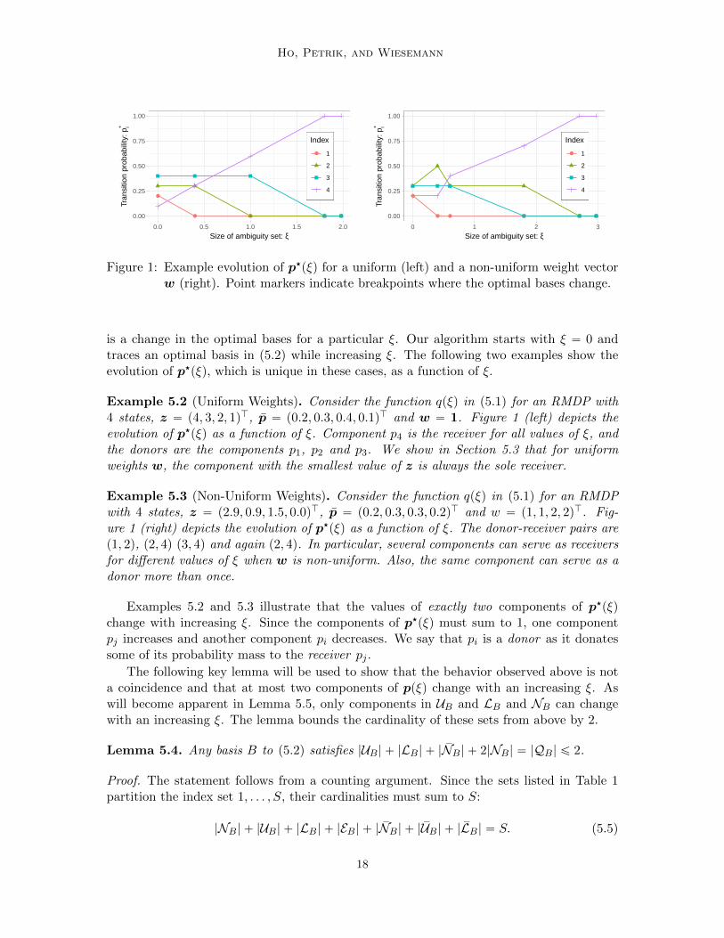
Figure 1: Example evolution of p‹pξq for a uniform (left) and a non-uniform weight vectorw (right). Point markers indicate breakpoints where the optimal bases change.
is a change in the optimal bases for a particular ξ. Our algorithm starts with ξ “ 0 andtraces an optimal basis in (5.2) while increasing ξ. The following two examples show theevolution of p‹pξq, which is unique in these cases, as a function of ξ.
Example 5.2 (Uniform Weights). Consider the function qpξq in (5.1) for an RMDP with4 states, z “ p4, 3, 2, 1qJ, p “ p0.2, 0.3, 0.4, 0.1qJ and w “ 1. Figure 1 (left) depicts theevolution of p‹pξq as a function of ξ. Component p4 is the receiver for all values of ξ, andthe donors are the components p1, p2 and p3. We show in Section 5.3 that for uniformweights w, the component with the smallest value of z is always the sole receiver.
Example 5.3 (Non-Uniform Weights). Consider the function qpξq in (5.1) for an RMDPwith 4 states, z “ p2.9, 0.9, 1.5, 0.0qJ, p “ p0.2, 0.3, 0.3, 0.2qJ and w “ p1, 1, 2, 2qJ. Fig-ure 1 (right) depicts the evolution of p‹pξq as a function of ξ. The donor-receiver pairs arep1, 2q, p2, 4q p3, 4q and again p2, 4q. In particular, several components can serve as receiversfor different values of ξ when w is non-uniform. Also, the same component can serve as adonor more than once.
Examples 5.2 and 5.3 illustrate that the values of exactly two components of p‹pξqchange with increasing ξ. Since the components of p‹pξq must sum to 1, one componentpj increases and another component pi decreases. We say that pi is a donor as it donatessome of its probability mass to the receiver pj .
The following key lemma will be used to show that the behavior observed above is nota coincidence and that at most two components of ppξq change with an increasing ξ. Aswill become apparent in Lemma 5.5, only components in UB and LB and NB can changewith an increasing ξ. The lemma bounds the cardinality of these sets from above by 2.
Lemma 5.4. Any basis B to (5.2) satisfies |UB| ` |LB| ` | sNB| ` 2|NB| “ |QB| ď 2.
Proof. The statement follows from a counting argument. Since the sets listed in Table 1partition the index set 1, . . . , S, their cardinalities must sum to S:
|NB| ` |UB| ` |LB| ` |EB| ` | sNB| ` | sUB| ` | sLB| “ S. (5.5)
18

Partial Policy Iteration for Robust MDPs
Each index i “ 1, . . . , S contributes between zero and two active constraints to the basis.For example, i P NB contributes no constraint, whereas i P sUB contributes 2 constraints.The requirement that B contains exactly 2S linearly independent constraints translates to
0 ¨ |NB| ` 1 ¨ |UB| ` 1 ¨ |LB| ` 2 ¨ |EB| ` 1 ¨ | sNB| ` 2 ¨ | sUB| ` 2 ¨ | sLB| ` |QB| “ 2S . (5.6)
Subtracting two times (5.5) from (5.6), we get
´2 ¨ |NB| ´ |UB| ´ |LB| ´ | sNB| ` |QB| “ 0 .
The result then follows by performing elementary algebra.
We next show that for any basis B feasible in (5.2) for a given ξ, the components in UBand LB act as donor-receiver pairs.
Lemma 5.5. Consider some ξ ą 0 and a basis B to problem (5.2) that is feasible in aneighborhood of ξ. Then the derivatives 9pi “
ddξ ppBpξqqi, i “ 1, . . . , S, and 9q “ d
dξ qBpξqsatisfy:
(C1) If UB “ tiu and LB “ tju, i ‰ j, then:
9q “zi ´ zjwi ` wj
, 9pi “1
wi ` wj, 9pj “ ´
1
wi ` wj.
(C2) If UB “ ti, ju, i ‰ j and wi ‰ wj, and LB “ H, then:
9q “zi ´ zjwi ´ wj
, 9pi “1
wi ´ wj, 9pj “ ´
1
wi ´ wj.
The derivatives 9p and 9q of all other types of feasible bases to problem (5.2) are zero.
The derivatives in the proposition exist since the functions pBpξq and qBpξq are linearfor any fixed basis B. The derivative 9p shows that in a basis of class (C1), i is the receiverand j is the donor. In a basis of class (C2), on the other hand, an inspection of 9p revealsthat i is the receiver and j is the donor whenever wi ą wj , and the reverse situation occurswhen wi ă wj .
Proof of Lemma 5.5. In this proof, we consider a fixed basis B and thus drop the subscriptB to reduce clutter. We also denote by xD the subvector of x P RS formed by the elementsxi, i P D, whose indices are contained in the set D Ď S.
First, observe that 9pi ‰ 0 is only possible if i P U Y L Y N . According to Table 1, ifi R U Y LYN , then i P E Y sU Y sLY sN . In the case where i P E , we have pi “ pi from thedefinition of E , and thus 9pi “ 0. If i P sU Y sL Y sN , then pi “ 0 from the definitions of thesets, and thus 9pi “ 0.
To derive the desired results, we consider the changes of q and p when we vary ξ in itsneighborhood with the same basis B, which by definition identifies the active constraintsin (5.2) even when ξ changes. Because at least two components of pBpξq need to changeas we vary ξ, we can restrict ourselves to bases B that satisfy |U | ` |L| ` |N | ě 2. SinceLemma 5.4 furthermore shows that |U | ` |L| ` 2|N | ď 2, we only need to consider threefollowing cases:
19
Ho, Petrik, and Wiesemann
(C1) |U | “ |L| “ 1 and |N | “ 0;(C2) |U | “ 2 and |L| “ |N | “ 0;(C3) |L| “ 2 and |U | “ |N | “ 0;
In the remainder of the proof, let p and l be the unique vectors that satisfy the activeconstraints in the basis B. Then, Table 1 implies the following useful equality that any pmust satisfy.
1 “ 1Jp “ 1JpN ` 1JpU ` 1JpL ` 1JpE ` 1JpĎN ` 1Jp
sU ` 1JpsL
“ 1JpN ` 1JpU ` 1JpL ` 1JpE(5.7)
Case (C1): U “ tiu, L “ tju, i ‰ j, and N “ H:Equation (5.7) implies that pi ` pj “ 1´ 1JpE and thus 9pi ` 9pj “ 0. We also have
wJl “ wJN lN `wJU lU `w
JL lL `w
JE lE `w
JĎN lĎN `w
JsU l sU `w
JsL l sL
“ wili ` wjlj `wJE lE `w
JsU l sU `w
JsL l sL
“ wili ` wjlj ´wJsU p sU `w
JsL p sL
“ wippi ´ piq ` wjppj ´ pjq ´wJsU p sU `w
JsL p sL ,
where the second identity follows from the fact that N “ H, U “ tiu and L “ tju byassumption, as well as sN “ H due to Lemma 5.4. The third identity holds since the activeconstraints in E , sU and sL imply that lE “ 0, l
sU “ ´p sU and lsL “ p sL, respectively. The last
identity, finally, is due to the fact that pi ´ pi “ li since i P U and pj ´ pj “ lj since j P L.Since any feasible basis B satisfies that wJl “ ξ, we thus obtain that
wippi ´ piq ` wjppj ´ pjq “ ξ `wJsU p sU ´w
JsL p sL
ùñ wi 9pi ´ wj 9pj “ 1 taking d{dξ on both sidesðñ wi 9pi ` wj 9pi “ 1 from 9pi ` 9pj “ 0ðñ 9pi “
1wi`wj
.
The expressions for 9pj and 9q follow from 9pi ` 9pj “ 0 and elementary algebra, respectively.Case (C2): U “ ti, ju, i ‰ j, and L “ N “ H:
Similar steps to case (C1) show that
wippi ´ piq ` wjppj ´ pjq “ ξ `wJsU p sU ´w
JsL p sL ,
which in turn yields the desired expressions for 9pi, 9pj and 9q. Note that if wi “ wj in theequation above, then the left hand side’s derivative with respect to ξ is zero, and we obtaina contradiction. This allows us to assume that wi ‰ wj in case (C2).
Case (C3): L “ ti, ju, i ‰ j, and U “ N “ H:Note that pL ď pL since lL satisfies both lL ě 0 and lL “ pL ´ pL. Since (5.7) impliesthat 1Jp “ 1JpL ` 1JpE “ 1, however, we conclude that pL “ pL, that is, we must have9p “ 0 and 9q “ 0.
5.2 Homotopy Algorithm
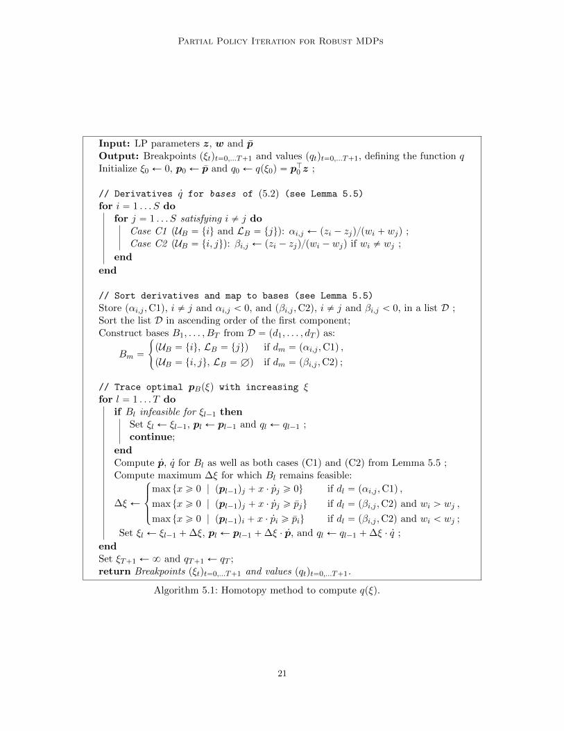
We are now ready to describe our homotopy method, which is presented in Algorithm 5.1.The algorithm starts at ξ0 “ 0 with the optimal solution p0 “ p achieving the objective
20
Partial Policy Iteration for Robust MDPs
Input: LP parameters z, w and pOutput: Breakpoints pξtqt“0,...T`1 and values pqtqt“0,...T`1, defining the function qInitialize ξ0 Ð 0, p0 Ð p and q0 Ð qpξ0q “ p
J0 z ;
// Derivatives 9q for bases of (5.2) (see Lemma 5.5)
for i “ 1 . . . S dofor j “ 1 . . . S satisfying i ‰ j do
Case C1 (UB “ tiu and LB “ tju): αi,j Ð pzi ´ zjq{pwi ` wjq ;Case C2 (UB “ ti, ju): βi,j Ð pzi ´ zjq{pwi ´ wjq if wi ‰ wj ;
end
end
// Sort derivatives and map to bases (see Lemma 5.5)
Store pαi,j ,C1q, i ‰ j and αi,j ă 0, and pβi,j ,C2q, i ‰ j and βi,j ă 0, in a list D ;Sort the list D in ascending order of the first component;Construct bases B1, . . . , BT from D “ pd1, . . . , dT q as:
Bm “
#
pUB “ tiu, LB “ tjuq if dm “ pαi,j ,C1q ,
pUB “ ti, ju, LB “ Hq if dm “ pβi,j ,C2q ;
// Trace optimal pBpξq with increasing ξfor l “ 1 . . . T do
if Bl infeasible for ξl´1 thenSet ξl Ð ξl´1, pl Ð pl´1 and ql Ð ql´1 ;continue;
endCompute 9p, 9q for Bl as well as both cases (C1) and (C2) from Lemma 5.5 ;Compute maximum ∆ξ for which Bl remains feasible:
∆ξ Ð
$
’
&
’
%
max tx ě 0 | ppl´1qj ` x ¨ 9pj ě 0u if dl “ pαi,j ,C1q ,
max tx ě 0 | ppl´1qj ` x ¨ 9pj ě pju if dl “ pβi,j ,C2q and wi ą wj ,
max tx ě 0 | ppl´1qi ` x ¨ 9pi ě piu if dl “ pβi,j ,C2q and wi ă wj ;
Set ξl Ð ξl´1 `∆ξ, pl Ð pl´1 `∆ξ ¨ 9p, and ql Ð ql´1 `∆ξ ¨ 9q ;
endSet ξT`1 Ð8 and qT`1 Ð qT ;return Breakpoints pξtqt“0,...T`1 and values pqtqt“0,...T`1.
Algorithm 5.1: Homotopy method to compute qpξq.
21
Ho, Petrik, and Wiesemann
value q0 “ pJ0 z. The algorithm subsequently traces each optimal basis as ξ increases,until the basis becomes infeasible and is replaced with the next basis. Since the functionqpξq is convex, it is sufficient to consider bases that have a derivative 9q that is no smallerthan the ones traced previously. Note that a basis of class (C1) satisfies UB “ tiu andLB “ tju for some receiver i P S and some donor j P S, j ‰ i, and this basis is feasibleat p “ p‹pξq, ξ ě 0, only if pi P rpi, 1s and pj P r0, pjs (see Lemma 5.5). Likewise, a basisof class (C2) satisfies UB “ ti, ju, i ‰ j, and LB “ H, and it is feasible at p “ p‹pξq,ξ ě 0, only if pi P rpi, 1s and pj P rpj , 1s. In a basis of class (C2), i is the receiver andj is the donor whenever wi ą wj , and the reverse situation occurs when wi ă wj . In thecase where 9qB1 “ 9qB2 for two different bases B1 and B2, the homotopy method would haveto inspect the solution trajectories of both bases as they can differ for larger values of ξ.This would increase the computational burden of the homotopy method. Assumption 5.1excludes these pathological cases by stipulating that all bases in Algorithm 5.1 have pairwisedifferent slopes 9q. As a by-product, the assumption guarantees that p‹pξq is unique for allξ since there is only one optimal sequence of bases, which implies that ppξq remains uniqueas ξ increases. Our implementation accounts for floating-point errors by using a queue tostore and examine the feasibility of all bases that are within some small ε of the last 9q.
Algorithm 5.1 generates the entire solution path of qpξq. Since qpξq is a piecewise linearfunction, the outputs of Algorithm 5.1 are the breakpoints of qpξq and their function values.If the goal is to compute the function q for a particular value of ξ, then we can terminate thealgorithm once the for loop over l has reached this value. In contrast, our bisection methodfor s-rectangular ambiguity sets (described in the next section) requires the entire solutionpath to compute robust Bellman policy updates. We also note that Algorithm 5.1 recordsall vectors p1, . . .pT . This is done for ease of exposition; for practical implementations, itis sufficient to only store the current iterate pl and update the two components that changein the “for loop” over l.
The following theorem proves the correctness of our homotopy algorithm. It shows thatthe function q is a piecewise linear function defined by the output of Algorithm 5.1.
Theorem 5.6. Let pξtqt“0,...,T`1 and pqtqt“0,...,T`1 be the output of Algorithm 5.1. Then,qpξq is a piecewise linear function with breakpoints ξl that satisfies qpξtq “ qt for t “0, . . . , T ` 1.
We prove the statement by contradiction. Since each point ql returned by Algorithm 5.1corresponds to the objective value of a feasible solution to problem (5.2) at ξ “ ξl, the outputgenerated by Algorithm 5.1 provides an upper bound on qpξq. Assume to the contrary thatthe output does not coincide point-wise with the function qpξq. In that case, there must bea value of ξ at which the homotopy method disregards a feasible basis that has a strictlysmaller derivative than the one selected. This, however, contradicts the way in which basesare selected by the algorithm.
Proof of Theorem 5.6. For ξ ď ξT , Algorithm 5.1 computes the piecewise linear function
gpξq “ minαP∆T`1
#
Tÿ
t“0
αt qt |Tÿ
t“0
αt ξt “ ξ
+
.
22
Partial Policy Iteration for Robust MDPs
To prove the statement, we show that gpξq “ qpξq for all ξ P r0, ξT s. Note that gpξq ě qpξqfor all ξ P r0, ξT s by construction since our algorithm only considers feasible bases. Also,from the construction of g, we have that qpξ0q “ gpξ0q for the initial point.
To see that gpξq ď qpξq, we need to show that Algorithm 5.1 does not skip any relevantbases. To this end, assume to the contrary that there exists a ξ1 P pξ0, ξT s such thatqpξ1q ă gpξ1q. Without loss of generality, there exists a value ξ1 such that that qpξq “ gpξqfor all breakpoints ξ ď ξ1 of q; this can always be achieved by choosing a sufficiently smallvalue of ξ1 where q and g differ. Let ξl be the largest element in tξt | t “ 0, . . . , T u suchthat ξl ă ξ1, that is, we have ξl ă ξ1 ď ξl`1. Such ξl exists because ξ1 ą ξ0 and qpξ0q “ gpξ0q.Let Bl be the basis chosen by Algorithm 5.1 for the line segment connecting ξl and ξl`1.We then observe that
9qpξ1q “qpξ1q ´ qlξ1 ´ ξl
ăgpξ1q ´ qlξ1 ´ ξl
“ql`1 ´ qlξl`1 ´ ξl
“ 9gpξ1q ,
where the first identity follows from our choice of ξ1, the inequality directly follows fromqpξ1q ă gpξ1q, and the last two identities hold since Bl is selected by Algorithm 5.1 for theline segment connecting ξl and ξl`1. However, by Lemmas 5.4 and 5.5, Bl is the basis withthe minimal slope between ξl and ξl`1, and it thus satisfies
ql`1 ´ qlξl`1 ´ ξl
ď 9qpξq ,
which contradicts the strict inequality above. The correctness of the last value ξT`1 “ 8,finally, follows since q is constant for large ξ as the constraint wJl “ ξ is inactive.
5.3 Complexity Analysis
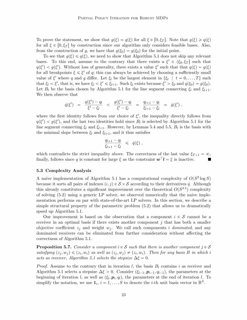
A naive implementation of Algorithm 5.1 has a computational complexity of OpS2 logSqbecause it sorts all pairs of indexes pi, jq P S ˆS according to their derivatives 9q. Althoughthis already constitutes a significant improvement over the theoretical OpS4.5q complexityof solving (5.2) using a generic LP solver, we observed numerically that the naive imple-mentation performs on par with state-of-the-art LP solvers. In this section, we describe asimple structural property of the parametric problem (5.2) that allows us to dramaticallyspeed up Algorithm 5.1.
Our improvement is based on the observation that a component i P S cannot be areceiver in an optimal basis if there exists another component j that has both a smallerobjective coefficient zj and weight wj . We call such components i dominated, and anydominated receivers can be eliminated from further consideration without affecting thecorrectness of Algorithm 5.1.
Proposition 5.7. Consider a component i P S such that there is another component j P Ssatisfying pzj , wjq ď pzi, wiq as well as pzj , wjq ‰ pzi, wiq. Then for any basis B in which iacts as receiver, Algorithm 5.1 selects the stepsize ∆ξ “ 0.
Proof. Assume to the contrary that in iteration l, the basis Bl contains i as receiver andAlgorithm 5.1 selects a stepsize ∆ξ ą 0. Consider pξl´1,pl´1, ql´1q, the parameters at thebeginning of iteration l, as well as pξl,pl, qlq, the parameters at the end of iteration l. Tosimplify the notation, we use 1i, i “ 1, . . . , S to denote the i-th unit basis vector in RS .
23
Ho, Petrik, and Wiesemann
Let k P S be the donor in iteration l. Note that k ‰ j as otherwise 9q ě 0, whichwould contradict the construction of the list D. Define δ via pl “ pl´1 ` δr1i ´ 1ks, andnote that δ ą 0 since ∆ξ ą 0. We claim that the alternative parameter setting pξ1l,p
1l, q
1lq
with p1l “ pl´1 ` δr1j ´ 1ks, ξ1l “ ‖p1l ´ p‖1,w and q1l “ z
Jp1l satisfies pξ1l, q1lq ď pξl, qlq and
pξ1l, q1lq ‰ pξl, qlq. Since this would correspond to a line segment with a steeper decrease
than the one constructed by Algorithm 5.1, this contradicts the optimality of Algorithm 5.1proved in Theorem 5.6. To see that pξ1l, q
1lq ď pξl, qlq, note that
ξ1l “∥∥p1l ´ p∥∥1,w
ď ‖pl ´ p‖1,w “ ξl
since wj ď wi and pi ě pi (otherwise, i could not be a receiver). Likewise, we have
q1l “ zJp1l ď zJpl “ ql
since zj ď zi. Finally, since pwi, ziq ‰ pwj , zjq, at least one of the previous two inequalitiesmust be strict, which implies that pξl,pl, qlq is not optimal, a contradiction.
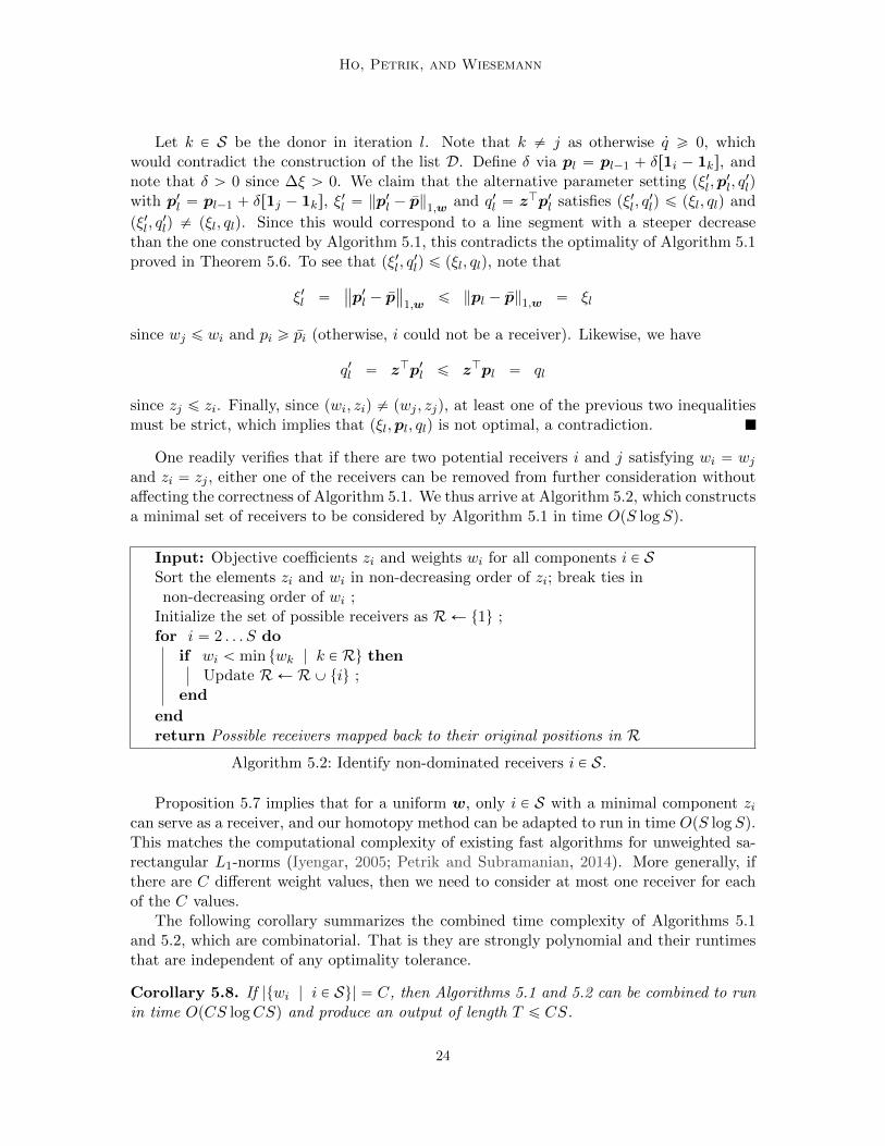
One readily verifies that if there are two potential receivers i and j satisfying wi “ wjand zi “ zj , either one of the receivers can be removed from further consideration withoutaffecting the correctness of Algorithm 5.1. We thus arrive at Algorithm 5.2, which constructsa minimal set of receivers to be considered by Algorithm 5.1 in time OpS logSq.
Input: Objective coefficients zi and weights wi for all components i P SSort the elements zi and wi in non-decreasing order of zi; break ties innon-decreasing order of wi ;
Initialize the set of possible receivers as RÐ t1u ;for i “ 2 . . . S do
if wi ă min twk | k P Ru thenUpdate RÐ RY tiu ;
end
endreturn Possible receivers mapped back to their original positions in R
Algorithm 5.2: Identify non-dominated receivers i P S.
Proposition 5.7 implies that for a uniform w, only i P S with a minimal component zican serve as a receiver, and our homotopy method can be adapted to run in time OpS logSq.This matches the computational complexity of existing fast algorithms for unweighted sa-rectangular L1-norms (Iyengar, 2005; Petrik and Subramanian, 2014). More generally, ifthere are C different weight values, then we need to consider at most one receiver for eachof the C values.
The following corollary summarizes the combined time complexity of Algorithms 5.1and 5.2, which are combinatorial. That is they are strongly polynomial and their runtimesthat are independent of any optimality tolerance.
Corollary 5.8. If |twi | i P Su| “ C, then Algorithms 5.1 and 5.2 can be combined to runin time OpCS logCSq and produce an output of length T ď CS.
24

Partial Policy Iteration for Robust MDPs
6. Computing the Bellman Operator: S-Rectangular Sets
We now develop a bisection scheme to compute the s-rectangular robust Bellman optimalityoperator L defined in (3.7). Our bisection scheme builds on the homotopy method for thesa-rectangular Bellman optimality operator described in the previous section.
The remainder of the section is structured as follows. We first describe the bisectionscheme for computing L in Section 6.1. Our method does not directly compute the greedypolicy required for our PPI from Section 4 but computes the optimal values of some dualvariables instead. Section 6.2 describes how to extract the optimal greedy policy from thesedual variables. Since our bisection scheme for computing L cannot be used to computethe s-rectangular robust Bellman policy update Lπ for a fixed policy π P Π, we describea different bisection technique for computing Lπ in Section 6.3. We use this technique tosolve the robust policy evaluation MDP defined in Section 4.
6.1 Bisection Scheme for Robust Bellman Optimality Operator
To simplify the notation, we fix a state s P S throughout this section and drop the associatedsubscripts whenever the context is unambiguous. In particular, we denote the nominaltransition probabilities under action a as pa P ∆S , the rewards under action a as ra P RS ,the L1-norm weight vector as wa P RS , and the budget of ambiguity as κ. We also fix avalue function v throughout this section. We then aim to solve the optimization problem
maxdP∆A
minξPRA
`
#
ÿ
aPAda ¨ qapξaq |
ÿ
aPAξa ď κ
+
, (6.1)
where qapξq is defined in (5.1) with subscript a P A to identify the associated action. Notethat problem (6.1) exhibits a very specific structure: It has a single constraint, and thefunction qa is piecewise linear with at most S2 pieces. We will use this structure to derivean efficient solution scheme that outperforms the naive solution of (6.1) via an LP solver.
Our bisection scheme employs the following reformulation of (6.1):
minuPR
#
u |ÿ
aPAq´1a puq ď κ
+
, (6.2)
where the inverse functions q´1a are defined as
q´1a puq “ min
pP∆S
}p´ pa}1,wa | pJz ď u
(
@a P A. (6.3)
Before we formally show that (6.1) and (6.2) are indeed equivalent, we discuss theintuition that underlies the formulation (6.2). In problem (6.1), the adversarial naturechooses the transition probabilities pa, a P A, to minimize the value of
ř
aPA da ¨ppJa zq while
adhering to the ambiguity budget viař
aPA ξa ď κ for ξa “ }pa´ pa}1,wa . In problem (6.3),q´1a puq can be interpreted as the minimum ambiguity budget }p ´ pa}1,wa assigned to the
action a P A that allows nature to ensure that taking an action a results in a robust valuepJz not exceeding u. Any value of u that is feasible in (6.2) thus implies that within thespecified overall ambiguity budget of κ, nature can ensure that every action a P A results
25

Ho, Petrik, and Wiesemann
●
●●
●
● ●●
uuuuuuuuuuuuuuuuuuu
ξ3ξ3ξ3ξ3ξ3ξ3ξ3ξ3ξ3ξ3ξ3ξ3ξ3ξ3ξ3ξ3ξ3ξ3ξ3 ξ2ξ2ξ2ξ2ξ2ξ2ξ2ξ2ξ2ξ2ξ2ξ2ξ2ξ2ξ2ξ2ξ2ξ2ξ2ξ1ξ1ξ1ξ1ξ1ξ1ξ1ξ1ξ1ξ1ξ1ξ1ξ1ξ1ξ1ξ1ξ1ξ1ξ1−1
0
1
2
3
0 1 2 3
Allocated ambiquity budget: ξa
Rob
ust Q
−fu
nctio
n: q
(ξa)
Function● q1
q2
q3
Figure 2: Visualization of the s-rectangular Bellman update with the response functionsq1, q2, q3 for 3 actions.
in a robust value not exceeding u. Minimizing u in (6.2) thus determines the transitionprobabilities that lead to the lowest robust value under any policy, which is the same ascomputing the robust Bellman optimality operator (6.1).
The following example demonstrates the relationship between q and q´1 as well as howthey are related to the optimization in (6.2).
Example 6.1. Figure 2 shows an example q-functions q1, q2, q3 for 3 actions. To achieve therobust value of u depicted in the figure, the smallest action-wise budgets ξa that guaranteeqpξaq ď u, i “ 1, 2, 3, are indicated at ξ1, ξ2 and ξ3, resulting in an overall budget ofκ “ ξ1 ` ξ2 ` ξ3.
We are now ready to state the main result of this section.
Theorem 6.2. The optimal objective values of (6.1) and (6.2) coincide.
Theorem 6.2 relies on the following auxiliary result, which we state first.
Lemma 6.3. The functions qa and q´1a are convex in ξ and u, respectively.
Proof. The convexity of qa is immediate from the LP formulation (5.2). The convexity ofq´1a can be shown in the same way by linearizing the objective function in (6.3).
Proof of Theorem 6.2. Since the functions qa, a P A, are convex (see Lemma 6.3), we canexchange the maximization and minimization operators in (6.1) to obtain
minξPRA
`
#
maxdP∆A
˜
ÿ
aPAda ¨ qapξaq
¸
|ÿ
aPAξa ď κ
+
.
26

Partial Policy Iteration for Robust MDPs
Since the inner maximization is linear in d, it is optimized at an extreme point of ∆A. Thisallows us to re-express the optimization problem as
minξPRA
`
#
maxaPA
tqapξaqu |ÿ
aPAξa ď κ
+
.
We can linearize the objective function in this problem by introducing the epigraphicalvariable u P R:
minuPR
minξPRA
`
#
u |ÿ
aPAξa ď κ, u ě max
aPAtqapξaqu
+
. (6.4)
It can be readily seen that for a fixed u in the outer minimization, there is an optimal ξ inthe inner minimization that minimizes each ξa individually while satisfying qapξaq ď u forall a P A. Define ga as the a-th component of this optimal ξ:
gapuq “ minξaPR`
tξa | qapξaq ď uu. (6.5)
We show that gapuq “ q´1a puq. To see this, we substitute qa in (6.5) to get:
gapuq “ minξaPR`
minpaP∆S
!
ξa | pJa za ď u, }pa ´ pa}1,wa
ď ξa
)
.
The identity ga “ q´1a then follows by realizing that the optimal ξ‹a in the equation above
must satisfy ξ‹a “ }pa ´ pa}1,wa. Finally, substituting the definition of ga in (6.5) into the
problem (6.4) shows that the optimization problem (6.1) is indeed equivalent to (6.2).
Input: Desired precision ε, functions q´1a , a P A
umin: maximum known u for which (6.2) is infeasible,umax: minimum known u for which (6.2) is feasible
Output: u such that |u‹ ´ u| ď ε, where u‹ is optimal in (6.2)while umax ´ umin ą 2 ε do
Split interval rumin, umaxs in half: uÐ pumin ` umaxq{2;Calculate the budget required to achieve the mid point u: sÐ
ř
aPA q´1a puq ;
if s ď κ thenu is feasible: update the feasible upper bound: umax Ð u;
elseu is infeasible: update the infeasible lower bound: umin Ð u;
end
endreturn pumin ` umaxq{2;
Algorithm 6.1: Bisection scheme for the robust Bellman optimality operator (3.7)
The bisection scheme for solving problem (6.2) is outlined in Algorithm 6.1. Bisection isa natural and efficient approach for solving the one-dimensional optimization problem. Thisalgorithm is simple and works well in practice, but it can be further improved by leveraging
27
Ho, Petrik, and Wiesemann
the fact that the functions q´1a , a P A, are piecewise linear. In fact, Algorithm 6.1 only
solves problem (6.2) to ε-optimality, and it requires the choice of a suitable precision ε.
We outline how to adapt Algorithm 6.1 to determine the optimal solution to prob-lem (6.2) in quasi-linear time independent of the precision ε; please see Algorithm B.1 inAppendix B for details. Recall that Algorithm 5.1 computes the breakpoints pξat qt“0,...,Ta`1,and objective values pqat qt“0,...,Ta`1, Ta ď S2, of each function qa, a P A. Then each inversefunction q´1
a is also piecewise linear with breakpoints pqat qt“0,...,Ta`1, and correspondingfunction values ξat “ q´1
a pqat q. Recall that we define q´1
a puq “ 8 for u ă qaTa`1. We nowcombine all breakpoints qat , a P A, to a single list K in ascending order. We then execute avariant of Algorithm 6.1 in which both umin and umax are always set to some breakpointsfrom K. Instead of choosing the midpoint uÐ pumin`umaxq{2 in each iteration of the bisec-tion, we choose the median breakpoint between umin and umax. Using the median insteadof the mean breakpoint reduces the method to a binary search which runs in logarithmictime. We stop once umin and umax are consecutive breakpoints in K, in which case theoptimal solution of (6.2) can be computed by basic algebra.
The following statement follows from the discussion above and the results in Appendix B.
Theorem 6.4. Algorithms 5.1 and 6.1 can be adapted (see Appendix B) to run jointly inOpS2A logSAq time, independent of the optimality tolerance.
Because each execution of Algorithm 6.1 requires that Algorithm 5.1 is executed toproduce its inputs, Theorem 6.4 states the joint complexity of the two algorithms. Usingreasoning similar to Corollary 5.8, the bound in Theorem 6.4 can be tightened as follows.
Corollary 6.5. If |twi | i P Su| “ C, then Algorithms 5.1, 5.2 and 6.1 can be adapted torun jointly in OpCSA logCSAq time, independent of the optimality tolerance.
We emphasize that general (interior-point) algorithms for the linear programming for-mulation of the robust Bellman optimality operator have a theoretical worst-case complexityof OpS4.5A4.5q (Karmarkar, 1984); see Appendix C. In addition, the spatial complexity ofour algorithms is OpS2Aq because we need to store at most S2 breakpoints for each action.Thus, the spatial complexity of our algorithms is linear in the input size since representinga dense transition function also takes OpS2Aq space.
6.2 Recovering the Greedy Policy
Since Algorithm 6.1 only computes the value of the robust Bellman optimality operator Land not an optimal greedy policy d‹ achieving this value, it cannot be used in PPI or relatedrobust policy iteration methods (Iyengar, 2005; Kaufman and Schaefer, 2013) as is. Thissection describes how to compute an optimal solution d‹ to problem (6.1) from the outputof Algorithm 6.1. We again fix a state s P S and drop the associated subscripts wheneverthe context is unambiguous. We also fix a value function v throughout this section. Finally,we assume that κ ą 0; the limiting case κ “ 0 is trivial since the robust Bellman optimalityoperator then reduces to the nominal Bellman optimality operator.
Recall that Algorithm 6.1 computes the optimal solution u‹ P R to problem (6.2), whichaccording to Theorem 6.2 equals the optimal value of problem (6.1). The same argument
28

Partial Policy Iteration for Robust MDPs
as in the proof of Theorem 6.2 thus implies that
u‹ “ maxdP∆A
minξPRA
`
#
ÿ
aPAda ¨ qapξaq |
ÿ
aPAξa ď κ
+
(6.6)
“ minξPRA
`
#
maxdP∆A
ÿ
aPAda ¨ qapξaq |
ÿ
aPAξa ď κ
+
. (6.7)
To compute an optimal d‹ from u‹, we first use the definition (6.3) of q´1a to compute ξ‹
defined asξ‹a “ q´1
a pu‹q @a P A . (6.8)
Intuitively, the components ξ‹a of this vector represent the action-wise uncertainty budgetsrequired to ensure that no greedy policy achieves a robust value that exceeds u‹. The setCpξ‹q “ ta P A | qapξ
‹aq “ u‹u of all actions achieving the optimal robust value plays an
important role in the construction of an optimal greedy policy d‹. To this end, the followingresult collects important properties of ξ‹ and Cpξ‹q.
Lemma 6.6. The vector ξ‹ defined in (6.8) is optimal in (6.7). Moreover, Cpξ‹q ‰ H and(i) qapξ
‹aq “ u‹ for all a P Cpξ‹q;
(ii) ξ‹a “ 0 and qapξ‹aq “ p
Ja z ď u‹ for all a P AzCpξ‹q.
Proof. We first argue that ξ‹ is optimal in (6.7). To see that ξ‹ is feasible in (6.7), fix anyoptimal solution ξ P RA in (6.7). The value qa1pξa1q can be upper bounded by the objectivein (6.7) as
qa1pξa1q ď maxdP∆A
ÿ
aPAda ¨ qapξaq ď u‹
for all a1 P A. The definition of qa in (5.1) implies that there are pa P ∆S , a P A, such that
pJa z ď u‹ and }pa ´ pa}1,wa ď ξa .
The definition of q´1a in (6.3) implies that each pa is feasible in q´1
a pu‹q. Thus, each ξ‹a is
bounded from above by ξa, and we observe thatÿ
aPAξ‹a ď
ÿ
aPAξa ď κ . (6.9)
Since the definition of q´1a also implies that ξ‹a “ q´1
a pu‹q ě 0, ξ‹ is indeed feasible in (6.7).
The optimality of ξ‹ in (6.7) then follows from the fact that qapξ‹aq ď u‹ because there
exists p‹a such that zJp‹a ď u‹ and }p‹a ´ pa}1,wa ď ξ‹a, by the definition of ξ‹a, a P A.Next, to show that Cpξ‹q ‰ H, note that for all a P A, we have
qapξ‹aq “ qapq
´1a pu
‹qq “ minp1P∆S
!
pJ1 z | }p1 ´ pa}1,waď minp2P∆S
!
}p2 ´ pa}1,wa| pJ2 z ď u‹
))
by the definitions of qa and q´1a in (5.1) and (6.3), respectively. Recognizing that any
optimal solution p‹2 to the inner minimization is feasible in the outer minimization leads to
qapξ‹aq ď pp‹2q
Jz ď u‹ .
29
Ho, Petrik, and Wiesemann
Given the inequality above, Cpξ‹q “ H only if qapξ‹aq ă u‹, for all a P A. Imagine now that
Cpξ‹q “ H. Then combining the equality in (6.6), the inequality in ξ‹ (6.9) and qapξ‹aq ă u‹
leads to
u‹ “ maxdP∆A
minξPRA
`
#
ÿ
aPAda ¨ qapξaq |
ÿ
aPAξa ď κ
+
ď maxdP∆A
ÿ
aPAda ¨ qapξ
‹aq ă u‹ ,
which is a contradiction.The statement (i) that qapξ
‹aq “ u‹ for all a P Cpξ‹q now follows immediately from the
definition of Cpξ‹q. To see that ξ‹a “ 0 for a P AzCpξ‹q in statement (ii), assume to thecontrary that ξ‹a ą 0 for some a P AzCpξ‹q. Since qapξ
‹aq ă u‹, there is p‹a P ∆S optimal
in (6.3) satisfying pp‹aqJz ă u‹ and }p‹a ´ pa}1,wa ď ξ‹a. At the same time, since ξ‹a ą 0,
we have }p‹a ´ pa}1,wa ą 0 as well. This implies, however, that there is ε ą 0 such thatp‹a ` ε ¨ ppa ´ p
‹aq is feasible in (6.3) and achieves a lower objective value than p‹a, which
contradicts the optimality of p‹a in (6.3). We thus conclude that ξ‹a “ 0 for a P AzCpξ‹q.This immediately implies that qapξ
‹aq “ p
Ja z for all a P AzCpξ‹q as well.
Finally, the fact stated in (ii) that qapξ‹aq ď u‹ for all a P AzCpξ‹q has already been
shown earlier in the proof.
The construction of d‹ P ∆A relies on the slopes of qa, which are piecewise constant butdiscontinuous at the breakpoints of qa. However, the functions qa are convex by Lemma 6.3,and therefore their subdifferentials (Rockafellar, 1970) Bqapξaq exist for all ξa ě 0. Usingthese subdifferentials, we construct optimal action probabilities d‹ P ∆A from ξ‹ as follows.
(i) If 0 P Bqapξ‹aq for some a P Cpξ‹q, define d‹ as
d‹a “
#
1 if a “ a
0 otherwise@a P A . (6.10a)
(ii) If 0 R Bqapξ‹aq for all a P Cpξ‹q, define d‹ as
d‹a “ea
ř
a1PA ea1with ea “
#
´ 1fa
if a P Cpξ‹q0 otherwise
@a P A , (6.10b)
where fa can be any element from Bqapξ‹aq, a P A.
The choice of d‹ may not be unique as there may be multiple a P Cpξ‹q that satisfy the firstcondition, and the choice of fa P Bqapξ
‹aq in the second condition may not be unique either.
Theorem 6.7. Any vector d‹ satisfying (6.10a) or (6.10b) is optimal in problem (6.1).Moreover, for ξ‹ defined in (6.8), pd‹, ξ‹q is a saddle point in (6.1).
Proof. One readily verifies that d‹ satisfying (6.10a) is contained in ∆A. To see that d‹ P ∆A
for d‹ satisfying (6.10b), we note that Cpξ‹q is non-empty due to Lemma 6.6 and that fa ă 0and thus ea ą 0 since qa is non-increasing. To see that d‹ satisfying (6.10a) or (6.10b) isoptimal in (6.1), we show that it achieves the optimal objective value u‹:
minξPRA
`
#
ÿ
aPAd‹a ¨ qapξaq |
ÿ
aPAξa ď κ
+
ě u‹ . (6.11)
30

Partial Policy Iteration for Robust MDPs
Observe that u‹ is indeed achieved for ξ “ ξ‹ sinceÿ
aPAd‹a ¨ qapξ
‹aq “
ÿ
aPCpξ‹qd‹a ¨ qapξ
‹aq “
ÿ
aPCpξ‹qd‹a ¨ u
‹ “ u‹ .
Here, the first equality holds since d‹a “ 0 for a R Cpξ‹q, the second equality follows fromthe definition of Cpξ‹q, and the third equality follows from d‹ P ∆A.
To establish the inequality (6.11), we show that ξ‹ is optimal in (6.11). This also provesthat pd‹, ξ‹q is a saddle point of problem (6.1). We denote by Bξpfqrξ
‹s the subdifferentialof a convex function f with respect to ξ, evaluated at ξ “ ξ‹. The KKT conditions for non-differentiable convex programs (see, for example, Theorem 28.3 of Rockafellar 1970), whichare sufficient for the optimality of ξ‹ in the minimization on the left-hand side of (6.11),require the existence of a scalar λ‹ ě 0 and a vector α‹ P RA` such that
0 P Bξ
˜
ÿ
aPAd‹a ¨ qapξaq ´ λ
‹
˜
κ´ÿ
aPAξa
¸
´ÿ
aPAα‹a ¨ ξa
¸
rξ‹s [Stationarity]
λ‹ ¨
˜
κ´ÿ
aPAξ‹a
¸
“ 0, α‹a ¨ ξ‹a “ 0 @a P A [Compl. Slackness]
The stationarity condition simplifies using the chain rule to
0 P d‹a ¨ Bqapξ‹aq ` λ
‹ ´ α‹a @a P A . (6.12)
If d‹ satisfies (6.10a), then both (6.12) and complementary slackness are satisfied forλ‹ “ 0 and α‹ “ 0. On the other hand, if d‹ satisfies (6.10b), we set
λ‹ “1
ř
aPCpξ‹q ea, α‹a “ 0 @a P Cpξ‹q, α‹a “ λ‹ @a P AzCpξ‹q ,
where ea is defined in (6.10b). This solution satisfies λ‹ ě 0 and α ě 0 because fa ď 0and therefore ea ě 0. This solution satisfies (6.12), and Lemma 6.6 implies that the secondcomplementary slackness condition is satisfied as well. To see that the first complementaryslackness condition is satisfied, we argue that
ř
aPA ξ‹a “ κ under the conditions of (6.10b).
Assume to the contrary thatř
aPA ξ‹a ă κ. Since 0 R Bqapξ
‹aq and the sets Bqapξ
‹aq are closed
for all a P Cpξ‹q (see page 215 and Theorem 23.4 of Rockafellar 1970), we have
Dβa ą 0 such that qapξ‹a ` βaq ă qapξaq @βa P p0, βaq
for all a P Cpξ‹q. We can thus marginally increase each component ξ‹a, a P Cpξ‹q, to obtaina new solution to problem (6.7) that is feasible and that achieves a strictly lower objectivevalue than u‹. This, however, contradicts the optimality of u‹. We thus conclude thatř
aPA ξ‹a “ κ, that is, the first complementary slackness condition is satisfied as well.
The values ξ‹ and d‹ can be computed in time OpA logSq since they rely on the quan-tities qapξ
‹aq and q´1
a pu‹q that have been computed previously by Algorithm 5.1 and Algo-
rithm 6.1, respectively. The worst-case transition probabilities can also be retrieved fromthe minimizers of qa defined in (5.1) since, as Theorem 6.7 implies, ξ‹ is optimal in theminimization problem in (6.1).
31

Ho, Petrik, and Wiesemann
6.3 Bisection Scheme for Robust Bellman Policy Update
Recall that the robust policy evaluation MDP pS, A,p0, p, r, γq defined in Section 4 hascontinuous action sets Apsq “ Ps, s P S, and the transition function p and the rewards rdefined as
ps,α “ÿ
aPAπs,a ¨αa and rs,α “ ´
ÿ
aPAπs,a ¨α
Ja rs,a .
To solve this MDP via value iteration or (modified) policy iteration, we must compute theBellman optimality operator L defined as
pLvqs “ maxαPPs
rs,α ` γ ¨ pJs,αv
(
“ maxαPp∆SqA
#
ÿ
aPAπs,a ¨α
Ja pγ ¨ v ´ rs,aq |
ÿ
aPA‖αa ´ ps,a‖1,ws,a ď κs
+
“ ´ minαPp∆SqA
#
ÿ
aPAπs,a ¨α
Ja prs,a ´ γ ¨ vq |
ÿ
aPA‖αa ´ ps,a‖1,ws,a ď κs
+
. (6.13)
The continuous action space in this MDP makes it impossible to compute Lv by simplyenumerating the actions. The ordinary Bellman operator could be solved as a linear pro-gram, but this suffers from the same computational limitations as its application to therobust Bellman operator described earlier. Using similar ideas as in Section 6.1, we canre-express the minimization problem in (6.13) as
minξPRA
`
#
ÿ
aPAπs,a ¨ qs,apξaq |
ÿ
aPAξa ď κs
+
, (6.14)
where the function qs,a : R` Ñ R is defined for each s P S and a P A as
qs,apξq “ minpP∆S
!
pJprs,a ´ γ ¨ vq | }p´ ps,a}1,ws,aď ξ
)
.
Note that this definition of qs,a corresponds to (5.1) with a different choice of z.At the first glance, problem (6.14) seems to be a special case of problem (6.1) from
Section 6.1, and one may posit that it can be solved using Algorithm 6.1. Unfortunately,this is not the case. The lack of optimization over d precludes the transformations employedin Theorem 6.2. However, problem (6.14) can still be solved efficiently by taking advantageof the fact that it only contains a single constraint on ξ and that the functions qs,a arepiecewise linear and convex. To see this, note that the Lagrangian of (6.14) is
maxλPR`
minξPRA
`
#
ÿ
aPApπs,a ¨ qs,apξaqq ` λ ¨ 1
Jξ ´ λκs
+
,
where the use of strong duality (Vanderbei, 1998) is justified since (6.14) can be reformulatedas a feasible linear program. The minimization can now be decomposed by actions:
maxλPR`
upλq “ maxλPR`
#
ÿ
aPAminξaPR`
tπs,a ¨ qs,apξaq ` λξau ´ λκs
+
(6.15)
32

Partial Policy Iteration for Robust MDPs
The inner minimization problems over ξa, a P A, are convex and can be solved exactly bybisection since the functions qs,a are piecewise linear. Likewise, the maximization over λcan be solved exactly by bisection since the function u is concave and piecewise linear. Thelower bound on λ for the bisection method is 0. A sufficient upper bound on λ is a value νsuch that ´ν ď Bξ qs,ap0q for all a P A. As can be readily seen from (6.15), upλq ď upνq forany λ ě ν. Finally, the optimal ξ in (6.14) can be recovered using a method similar to theone described in Section 6.2.
7. Numerical Evaluation
We now compare the runtimes of PPI (Algorithm 4.1) combined with the homotopy method(Algorithm 5.1) and the bisection method (Algorithm 6.1) with the runtime of a naiveapproach that combines the robust value iteration with a computation of the robust Bellmanoptimality operator L using a general LP solver. We use Gurobi 9.0, a state-of-the-artcommercial optimization package. All algorithms were implemented in C++, parallelizedusing the OpenMP library, and used the Eigen library to perform linear algebra operations.The algorithms were compiled with GCC 9.3 and executed on an AMD Ryzen 9 3900X CPUwith 64GB RAM. The source code of the implementation is available at http://github.
com/marekpetrik/craam2.
7.1 Experimental Setup
Our experiments involve two problems from different domains with a fundamentally differentstructure. The two domains are the inventory management problem (Zipkin, 2000; Porteus,2002) and the cart-pole problem (Lagoudakis and Parr, 2003). The inventory managementproblem has many actions and dense transition probabilities. The cart-pole problem, onthe other hand, has only two actions and sparse transition probabilities. More actions anddense transition probabilities make for much more challenging computation of the Bellmanupdate compared to policy evaluation.
Next, we give a high-level description of both problems as well as our parameter choice.Because the two domains serve simply as benchmark problems and their full descriptionwould be lengthy, we only outline their motivation, construction, and properties. To fa-cilitate the reproducibility of the domains, CSV files with the precise specification of theRMDPs being solved are available at http://github.com/marekpetrik/PPI_paper.
In our inventory management problem, a retailer orders, stores and sells a single productover an infinite time horizon. Any orders submitted in a time period t are fulfilled at thebeginning of time period t`1 and are subject to deterministic fixed and variable costs. Anyitems held in the limited-capacity inventory incur deterministic per-period holding costs.The per-unit sales price is deterministic, but the per-period demand is stochastic. Allaccrued demand in time period t is satisfied up to the available inventory. Any remainingunsatisfied demand is backlogged at a per-unit backlogging penalty up to a given limit.The states and actions of our MDP represent the inventory levels and the order quantitiesin any given time period, respectively. The stochastic demands drive the stochastic statetransitions. The rewards are the sales revenue minus the purchase costs in each period.
In our experiments, the fixed and variable ordering costs are 5.99 and 1.0, respectively.The inventory holding and backlogging costs are 0.1 and 0.15, respectively. We vary the
33
Ho, Petrik, and Wiesemann
inventory capacity I to study the impact of the problem’s size on the runtimes, while thebacklog limit is I{3. We also impose an upper limit of I{2 on each order. The correspondingMDP thus has I ` I{3 “ 4{3 ¨ I states and I{2 actions. Note that due to the inventorycapacity limits, not all actions are available at every state. The unit sales price is 1.6. Thedemand in each period follows the Gaussian distribution with a mean of I{2 and a standarddeviation of I{5 and is rounded to the closest integer. We use a discount factor of 0.995.
In our cart-pole problem, a pole has to be balanced upright on top of a cart that movesalong a single dimension. At any point in time, the state of the system is described byfour continuous quantities: the cart’s position and velocity, as well as the pole’s angle andangular velocity. To balance the pole, one can apply a force to the cart from the left or fromthe right. The resulting MDP thus accommodates a 4-dimensional continuous state spaceand two actions. Several different implementations of this problem can be found in theliterature; in the following, we employ the deterministic implementation from the OpenAIGym. Again, we use a discount factor of 0.995.
Since the state space of our cart-pole problem is continuous, we discretize it to beamenable to our solution methods. The discretization follows a standard procedure inwhich random samples from the domain are subsampled to represent the discretized statespace. The transitions are then estimated from samples that are closest to each state. Inother words, the probability of transitioning from a discretized state s to another discretizedstate s1 is proportional to the number of sampled transitions that originate near s and endup near s1. The discretized transition probabilities are no longer deterministic, even thoughthe original problem transitions are.
The ambiguity sets are modified slightly in this section to ensure a more realistic eval-uation. Assuming that the robust transition can be positive to any state of the RMDPcan lead to overly conservative policies. To obtain less conservative policies, we restrict ourambiguity sets Ps,a and Ps from Section 3 to probability distributions that are absolutelycontinuous with respect to the nominal distributions ps,a. Our sa-rectangular ambiguitysets Ps,a thus become
Ps,a “
p P ∆S | }p´ ps,a}1,ws,a ď κs,a, ps1 ďP
ps,a,s1T
@s1 P S(
,
and we use a similar construction for our s-rectangular ambiguity sets Ps. We set theambiguity budget to κs,a “ 0.2 and κs “ 1.0 in the sa-rectangular and s-rectangular versionof our inventory management problem, respectively, and we set κs,a “ κs “ 0.1 in our cart-pole problem. Anecdotally, the impact of the ambiguity budget on the runtimes is negligible.We report separate results for uniform weights ws,a “ 1 and non-uniform weights ws,a thatare derived from the value function v. In the latter case, we choose weights pws,aqs1 that areproportional to |vs1 ´ 1Jv{S|, which have been shown to optimize the percentile criterionfor uncertain MDPs (Behzadian et al., 2021). All weights ws,a are normalized so that theirvalues are contained in r0, 1s. Note that the simultaneous scaling of ws,a and κs,a does notaffect the solution.
Recall that the policy evaluation step in PPI can be accomplished by any MDP solu-tion method. In our inventory management problem, whose instances have up to 1, 000states, we use policy iteration and solve the arising systems of linear equations via theLU decomposition of the Eigen library (Puterman, 2005). This approach does not scalewell to MDPs with S " 1, 000 states as the policy iteration manipulates matrices of di-
34
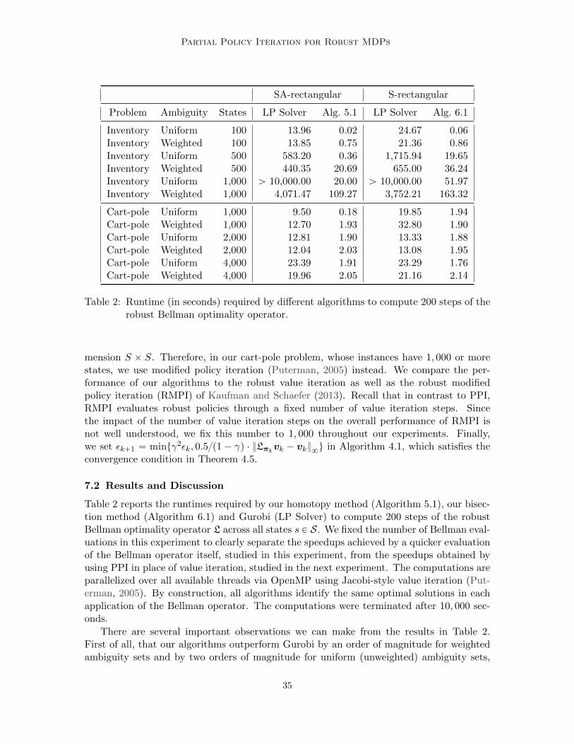
Partial Policy Iteration for Robust MDPs
SA-rectangular S-rectangular
Problem Ambiguity States LP Solver Alg. 5.1 LP Solver Alg. 6.1
Inventory Uniform 100 13.96 0.02 24.67 0.06Inventory Weighted 100 13.85 0.75 21.36 0.86Inventory Uniform 500 583.20 0.36 1,715.94 19.65Inventory Weighted 500 440.35 20.69 655.00 36.24Inventory Uniform 1,000 ą 10,000.00 20.00 ą 10,000.00 51.97Inventory Weighted 1,000 4,071.47 109.27 3,752.21 163.32
Cart-pole Uniform 1,000 9.50 0.18 19.85 1.94Cart-pole Weighted 1,000 12.70 1.93 32.80 1.90Cart-pole Uniform 2,000 12.81 1.90 13.33 1.88Cart-pole Weighted 2,000 12.04 2.03 13.08 1.95Cart-pole Uniform 4,000 23.39 1.91 23.29 1.76Cart-pole Weighted 4,000 19.96 2.05 21.16 2.14
Table 2: Runtime (in seconds) required by different algorithms to compute 200 steps of therobust Bellman optimality operator.
mension S ˆ S. Therefore, in our cart-pole problem, whose instances have 1, 000 or morestates, we use modified policy iteration (Puterman, 2005) instead. We compare the per-formance of our algorithms to the robust value iteration as well as the robust modifiedpolicy iteration (RMPI) of Kaufman and Schaefer (2013). Recall that in contrast to PPI,RMPI evaluates robust policies through a fixed number of value iteration steps. Sincethe impact of the number of value iteration steps on the overall performance of RMPI isnot well understood, we fix this number to 1, 000 throughout our experiments. Finally,we set εk`1 “ mintγ2εk, 0.5{p1 ´ γq ¨ }Lπk
vk ´ vk}8u in Algorithm 4.1, which satisfies theconvergence condition in Theorem 4.5.
7.2 Results and Discussion
Table 2 reports the runtimes required by our homotopy method (Algorithm 5.1), our bisec-tion method (Algorithm 6.1) and Gurobi (LP Solver) to compute 200 steps of the robustBellman optimality operator L across all states s P S. We fixed the number of Bellman eval-uations in this experiment to clearly separate the speedups achieved by a quicker evaluationof the Bellman operator itself, studied in this experiment, from the speedups obtained byusing PPI in place of value iteration, studied in the next experiment. The computations areparallelized over all available threads via OpenMP using Jacobi-style value iteration (Put-erman, 2005). By construction, all algorithms identify the same optimal solutions in eachapplication of the Bellman operator. The computations were terminated after 10, 000 sec-onds.
There are several important observations we can make from the results in Table 2.First of all, that our algorithms outperform Gurobi by an order of magnitude for weightedambiguity sets and by two orders of magnitude for uniform (unweighted) ambiguity sets,
35

Ho, Petrik, and Wiesemann
SA-rectangular S-rectangular
Problem Ambiguity States VI RMPI PPI VI PPI
Inventory Uniform 100 0.12 0.03 0.01 3.52 0.15Inventory Weighted 100 10.28 0.94 0.14 15.02 1.02Inventory Uniform 500 1.39 0.06 0.14 24.69 2.71Inventory Weighted 500 140.53 5.69 2.11 276.63 16.76Inventory Uniform 1,000 8.65 0.23 0.59 217.90 13.98Inventory Weighted 1,000 393.90 14.36 6.90 519.21 163.18
Cart-pole Uniform 1,000 0.03 0.06 0.03 0.80 0.15Cart-pole Weighted 1,000 0.25 0.17 0.04 0.98 0.28Cart-pole Uniform 10,000 0.32 0.26 0.13 8.40 1.06Cart-pole Weighted 10,000 1.72 1.13 0.21 13.43 3.52Cart-pole Uniform 20,000 0.44 0.54 0.29 16.24 2.40Cart-pole Weighted 20,000 6.37 3.22 0.62 28.50 9.30
Table 3: Runtime (in seconds) required by different algorithms to compute an approxi-mately optimal robust value function.
independent of the type of rectangularity. This impressive performance is because theinventory management problem has many actions, which makes computing the Bellmanoperator particularly challenging. The computation time also reflects that homotopy andbisection methods have quasi-linear time complexities when used with uniform L1 norms.It is remarkable that even with the simple cart-pole problem our algorithms are about10 to 20 times faster than a state-of-the-art LP solver. In fact, our results indicate thateven moderately-sized RMDPs may be practically intractable when solved with generic LPsolvers.
Table 3 reports the runtimes required by the parallelized versions of the robust valueiteration (VI), the robust modified policy iteration (RMPI) and our partial policy iteration(PPI) to solve our inventory management and cart-pole problems to approximate optimality.To this end, we choose a precision of δ “ 40 (that is, }Lπk
vk ´ vk}8 ď 0.1), as definedin Algorithm 4.1, for our inventory management problem, as well as a smaller precisionof δ “ 4 (that is, }Lπk
vk ´ vk}8 ď 0.01) for our cart-pole problem, to account for thesmaller rewards in this problem. All algorithms use the homotopy (Algorithm 5.1) andthe bisection method (Algorithm 6.1) to compute the robust Bellman optimality operator.Note that RMPI is only applicable to sa-rectangular ambiguity sets. The computationswere terminated after 10, 000 seconds.
There are also several important observations we can make from the results in Table 3.As one would expect, PPI in RMDPs behaves similarly to policy iteration in MDPs. It out-performs value iteration in essentially all benchmarks, being almost up to 100 times faster,but the margin varies significantly. The improvement margin depends on the relative com-plexity of policy improvements and evaluations. In the sa-rectangular cart-pole problem,for example, the policy improvement step is relatively cheap, and thus the benefit of em-
36
Partial Policy Iteration for Robust MDPs
ploying a policy evaluation is small. The situation is reversed in the s-rectangular inventorymanagement problem, in which the policy improvement step is very time-consuming. PPIoutperforms the robust value iteration most significantly in the sa-rectangular inventorymanagement problem since the policy evaluation step is much cheaper than the policy im-provement step due to the large number of available actions. RMPI’s performance, on theother hand, is more varied: while it sometimes outperforms the other methods, it is usu-ally dominated by at least one of the competing algorithms. We attribute this fact to theinefficient value iteration that is employed in the robust policy evaluation step of RMPI.It is important to emphasize that PPI has the same theoretical convergence rate as therobust value iteration, and thus its performance relative to the robust value iteration andRMPI will depend on the specific problem instance and as well as the employed parametersettings.
In conclusion, our empirical results show that our proposed combination of PPI and thehomotopy or bisection method achieves a speedup of up to four orders of magnitude for bothsa-rectangular and s-rectangular ambiguity sets when compared with the state-of-the-artsolution approach that combines a robust value iteration with a computation of the robustBellman operator via a commercial LP solver. Since our methods scale more favorably withthe size of the problem, their advantage is likely to only increase with larger problems thatwhat we considered here.
8. Conclusion
We proposed three new algorithms to solve robust MDPs over L1-ball uncertainty sets.Our homotopy algorithm computes the robust Bellman operator over sa-rectangular L1-balluncertainty sets in quasi-linear time and is thus almost as efficient as computing the ordinaryBellman operator. Our bisection scheme utilizes the homotopy algorithm to compute therobust Bellman operator over s-rectangular L1-ball uncertainty sets, again in quasi-lineartime. Both algorithms can be combined with PPI, which generalizes the highly efficientmodified policy iteration scheme to robust MDPs. Our numerical results show significantspeedups of up to four orders of magnitude over a leading LP solver for both sa-rectangularand s-rectangular ambiguity sets.
Our research opens up several promising avenues for future research. First, our homo-topy method sorts the bases of problem (5.2) in quasi-linear time. This step could also beimplemented in linear time using a variant of the quickselect algorithm, which has led toimprovements in a similar context (Condat, 2016). Second, we believe that the techniquespresented here can be adapted to other uncertainty sets, such as L8- and L2-balls aroundthe nominal transition probabilities or uncertainty sets based on φ-divergences. Both theefficient implementation of the resulting algorithms as well as the empirical comparison ofdifferent uncertainty sets on practical problem instances would be of interest. Third, itis important to study how our methods generalize to robust value function approximationmethods (Tamar et al., 2014). Finally, we believe that the study of robust MDPs under theaverage reward setting is another interesting direction for future research.
37

Ho, Petrik, and Wiesemann
Acknowledgments
We thank Bruno Scherrer for pointing out the connections between policy iteration andalgorithms for solving zero-sum games and Stephen Becker for insightful comments. Thiswork was supported by the National Science Foundation under Grants No. IIS-1717368and IIS-1815275, by the Engineering and Physical Sciences Research Council under GrantNo. EP/R045518/1, by the City University of Hong Kong (Project No. 9610481 and7005534), and by the National Natural Science Foundation of China (Project No. 72032005).Any opinions, findings, and conclusions or recommendations are those of the authors anddo not necessarily reflect the views of the funding bodies.
Appendix A. Properties of Robust Bellman Operator
We prove several fundamental properties of the robust Bellman policy update Lπ and therobust Bellman optimality operator L over s-rectangular and sa-rectangular ambiguity sets.
Lemma A.1. For both s-rectangular and sa-rectangular ambiguity sets, the robust Bellmanpolicy update Lπ and the robust Bellman optimality operator L are γ-contractions under theL8-norm, that is
}Lπx´ Lπy}8 ď γ }x´ y}8 and }Lx´ Ly}8 ď γ }x´ y}8 .
The equations Lπv “ v and Lv “ v have the unique solutions vπ and v‹, respectively.
Proof. See Theorem 3.2 of Iyengar (2005) for sa-rectangular sets and Theorem 4 of Wiese-mann et al. (2013) for s-rectangular sets.
Lemma A.2. For both s-rectangular and sa-rectangular ambiguity sets, the robust Bellmanpolicy update Lπ and the robust Bellman optimality operator L are monotone:
Lπx ě Lπy and Lx ě Ly @x ě y .
Proof. We show the statement for s-rectangular ambiguity sets; the proof of sa-rectangularuncertainty sets is analogous. Consider π P Π as well as x,y P RS such that x ě y anddefine
Fspp,xq “ÿ
aPAπs,a ¨ p
Ja prs,a ` γ ¨ xq .
The monotonicity of the robust Bellman policy update Lπ follows from the fact that
pLπxqs “ minpPPs
Fspp,xq “ Fspp‹,xq ě Fspp
‹,yq(a)ě pLπyqs @s P S ,
where p‹ P arg minpPPsFspp,xq. The inequality (a) holds because Fspp
‹, ¨q is monotonesince p‹ ě 0.
To prove the monotonicity of the robust Bellman optimality operator L, consider againsome x and y with x ě y and let π‹ be the greedy policy satisfying Ly “ Lπ‹y. We thenhave that
pLyqs “ pLπ‹yqs ď pLπ‹xqs ď pLxqs,
where the inequalities follow from the (previously shown) monotonicity of Lπ‹ and the factthat pLxqs “ pmaxπPΠ Lπxqs ě pLπ‹xqs.
38
Partial Policy Iteration for Robust MDPs
Lemmas A.1 and A.2 further imply the following two properties of Lπ and L.
Corollary A.3. For both s-rectangular and sa-rectangular ambiguity sets, the robust Bell-man policy update Lπ and the robust Bellman optimality operator L satisfy v‹ ě vπ foreach π P Π.
Proof. The corollary follows from the monotonicity (Lemma A.2) and contraction properties(Lemma A.1) of L and Lπ using standard arguments. See, for example, Proposition 2.1.2in Bertsekas (2013).
Corollary A.4. For both s-rectangular and sa-rectangular ambiguity sets, the robust Bell-man policy update Lπ and the robust Bellman optimality operator L satisfy for any v P RSthat
}v‹ ´ v}8 ď1
1´ γ}Lv ´ v}8 and }vπ ´ v}8 ď
1
1´ γ}Lπv ´ v}8 .
Proof. The corollary follows from the monotonicity (Lemma A.2) and contraction properties(Lemma A.1) of L and Lπ using standard arguments. See, for example, Proposition 2.1.1in Bertsekas (2013).
We next show that both Lπ and L are invariant when adding a constant to the valuefunction.
Lemma A.5. For both s-rectangular and sa-rectangular ambiguity sets, the robust Bellmanpolicy update Lπ and the robust Bellman optimality operator L are translation invariant foreach π P Π:
Lπpv ` ε ¨ 1q “ Lπv ` γε ¨ 1 and Lpv ` ε ¨ 1q “ Lv ` γε ¨ 1 @v P RS , @ε P R
Proof. We show the statement for s-rectangular ambiguity sets; the proof of sa-rectangularuncertainty sets is analogous. Fixing π P Π, v P RS and ε P R, we have
pLπpv ` ε1qqs “ minpPPs
ÿ
aPAπs,a ¨ p
Ja prs,a ` γ ¨ rv ` ε ¨ 1sq
“ minpPPs
ÿ
aPAπs,a ¨ pp
Ja prs,a ` γ ¨ vq ` γεq
“ γε` minpPPs
ÿ
aPAπs,a ¨ p
Ja prs,a ` γ ¨ vq ,
where the first identity holds by definition of Lπ, the second is due to the fact that pJa 1 “ 1since Ps Ď p∆SqA, and the third follows from the fact that
ř
aPA πs,a “ 1.To see that Lpv ` ε ¨ 1q “ Lv ` γε ¨ 1, we note that
Lpv ` ε ¨ 1q “ Lπ1pv ` ε ¨ 1q “ Lπ1v ` γε ¨ 1 ď Lv ` γε ¨ 1 ,
where π1 P Π is the greedy policy that satisfies Lπ1pv ` ε ¨ 1q “ Lpv ` ε ¨ 1q, as well as
Lv ` γε ¨ 1 “ Lπ2v ` γε ¨ 1 “ Lπ2pv ` ε ¨ 1q ď Lpv ` ε ¨ 1q ,
where π2 P Π is the greedy policy that satisfies Lπ2v “ Lv.
39
Ho, Petrik, and Wiesemann
Our last result in this section shows that the difference between applying the robustBellman policy update Lπ to two value functions can be bounded from below by a linearfunction.
Lemma A.6. For both s-rectangular and sa-rectangular ambiguity sets, there exists astochastic matrix P such that the robust Bellman policy update Lπ satisfies
Lπx´ Lπy ě γ ¨ P px´ yq ,
for each π P Π and x,y P RS.
Proof. We show the statement for s-rectangular ambiguity sets; the proof of sa-rectangularuncertainty sets is analogous. We have that
pLπx´ Lπyqs “ minpPPs
#
ÿ
aPAπs,a ¨ p
Ja prs,a ` γ ¨ xq
+
´ minpPPs
#
ÿ
aPAπs,a ¨ p
Ja prs,a ` γ ¨ yq
+
ě minpPPs
#
ÿ
aPA
`
πs,a ¨ pJa prs,a ` γ ¨ xq
˘
´ÿ
aPA
`
πs,a ¨ pJa prs,a ` γ ¨ yq
˘
+
“ minpPPs
#
ÿ
aPAπs,a ¨ γ ¨ p
Ja px´ yq
+
.
The result follows by constructing a stochastic matrix P such that its s-th row isř
aPA πs,a ¨pJa where pa is the optimizer in the last minimization above.
Appendix B. Bisection Algorithm with Quasi-Linear Time Complexity
We adapt Algorithm 6.1 to determine the optimal solution to problem (6.2) in quasi-lineartime without dependence on any precision ε. Recall that Algorithm 5.1 computes thebreakpoints pξat qt, t “ 0, . . . , Ta` 1 and objective values pqat qt, t “ 0, . . . , Ta` 1, Ta ď S2, ofeach function qa, a P A. Moreover, each inverse function q´1
a is also piecewise linear withbreakpoints pqat qt, t “ 0, . . . , Ta` 1 and corresponding function values ξat “ q´1
a pqat q, as well
as q´1a puq “ 8 for u ă qaTa`1. We use this data as input for our revised bisection scheme in
Algorithm B.1.
Algorithm B.1 first combines all breakpoints qat , t “ 0, . . . Ta`1 and a P A, of the inversefunctions q´1
a , a P A, to a single list K in ascending order. It then bisects on the indices ofthese breakpoints. The result is a breakpoint pair pkmin, kmaxq satisfying kmax “ kmin ` 1as well as κ P
“ř
aPA q´1a pqkmin
q,ř
aPA q´1a pqkmaxq
‰
. Since none of the functions q´1a have a
breakpoint between qkminand qkmax , finding the optimal solution u‹ to problem (3.7) then
reduces to solving a single linear equation in one unknown, which is done in the last partof Algorithm B.1.
The complexity of Algorithm B.1 is dominated by the merging of the sorted listspqat qt“0,...Ta`1, a P A, as well as the computation of s inside the while-loop. Merging Asorted lists, each of size less than or equal to CS, can be achieved in time OpCSA logAq.However, each one of these lists needs to be also sorted in Algorithm 5.1 giving the overallcomplexity of OpCSA logCSAq. Then, computing q´1
a at a given point can be achieved in
40

Partial Policy Iteration for Robust MDPs
Input: Breakpoints pqat qt“0,...,Ta`1, of all functions qa, a P AOutput: The optimal solution u‹ to the problem (6.2)Combine qat , t “ 0, . . . , Ta and a P A, to a single list K “ pq1, . . . , qKq in ascendingorder, omitting any duplicates ;
// Bisection search to find the optimal line segment pkmin, kmaxq
kmin Ð 1; kmax Ð K ;while kmax ´ kmin ą 1 do
Split tkmin, . . . , kmaxu in half: k Ð roundppkmin ` kmaxq{2q ;Calculate the budget required to achieve u “ qk: sÐ
ř
aPA q´1a pqkq ;
if s ď κ thenu “ qk is feasible: update the feasible upper bound: kmax Ð k ;
elseu “ qk is infeasible: update the infeasible lower bound: kmin Ð k ;
end
end
// All q´1a are affine on pqkmin
, qkmaxq
umin Ð qkmin; umax Ð qkmax ;
smin Ðř
aPA q´1a puminq; smax Ð
ř
aPA q´1a pumaxq ;
αÐ pκ´ sminq{psmax ´ sminq ;u‹ Ð p1´ αq ¨ umin ` α ¨ umax;return u‹
Algorithm B.1: Quasi-linear time bisection scheme for solving (3.7)
41

Ho, Petrik, and Wiesemann
time OplogCSq, so that s in an individual iteration of the while-loop can be computed intime OpA logCSq. Since the while-loop is executed OplogCSAq many times, computing shas an overall complexity of OpA logCS logCSAq. We thus conclude that Algorithm B.1has a complexity of OpCSA logA`A logCS logCSAq.
Appendix C. Computing the Bellman Operator via Linear Programming
In this section we present an LP formulation for the robust s-rectangular Bellman optimalityoperator L defined in (3.7):
pLvqs “ maxdP∆A
minpPp∆SqA
#
ÿ
aPAda ¨ p
Ja za |
ÿ
aPA‖pa ´ ps,a‖1,ws,a ď κs
+
Here, we use za “ rs,a`γ ¨v in the objective function. Employing an epigraph reformulation,the inner minimization problem can be re-expressed as the following linear program:
minimizepPRAˆS ,θPRAˆS
ÿ
aPAda ¨ z
Ja pa
subject to 1Jpa “ 1 @a P A rxas
pa ´ pa ě ´θa @a P A ryna s
pa ´ pa ě ´θa @a P A rypas
´ÿ
aPAwJa θa ě ´κ rλs
p ě 0, θ ě 0
For ease of exposition, we have added the dual variables corresponding to each constraintin brackets. This linear program is feasible by construction, which implies that its optimalvalue coincides with the optimal value of its dual. We can thus dualize this linear programand combine it with the outer maximization to obtain the following linear programmingreformulation of the the robust s-rectangular Bellman optimality operator L:
maximizedPRA,xPRA, λPRypPRSˆA,ynPRSˆA
ÿ
aPA
´
xa ` pJa ry
na ´ y
pas
¯
´ κ ¨ λ
subject to 1Jd “ 1, d ě 0
´ypa ` yna ` x ¨ 1 ď daza @a P A
ypa ` yna ´ λ ¨wa ď 0 @a P A
yp ě 0 yn ě 0
λ ě 0
This problem has OpSAq variables and an input bitlength of OpSAq. As such, its theoreticalruntime complexity is OpS4.5A4.5q (Karmarkar, 1984).
References
M. S. Asif and J. Romberg. Dantzig selector homotopy with dynamic measurements. InIS&T/SPIE Computational Imaging, 2009.
42

Partial Policy Iteration for Robust MDPs
B. Behzadian, R. Russel, M. Petrik, and C. P. Ho. Optimizing percentile criterion us-ing robust MDPs. In International Conference on Artificial Intelligence and Statistics(AISTATS), 2021.
D. P. Bertsekas. Abstract Dynamic Programming. Athena Scientific, 2013.
D. Bertsimas and J. N. Tsitsiklis. Introduction to Linear Optimization. Athena Scientific,1997.
L. Condat. Fast projection onto the Simplex and the l1 ball. Mathematical Programming,158(1-2):575–585, 2016.
A. Condon. On algorithms for simple stochastic games. Advances in Computational Com-plexity Theory, DIMACS Series in Discrete Mathematics and Theoretical Computer Sci-ence, 13:51–71, 1993.
K. V. Delgado, L. N. De Barros, D. B. Dias, and S. Sanner. Real-time dynamic programmingfor Markov decision processes with imprecise probabilities. Artificial Intelligence, 230:192–223, 2016.
E. Derman, D. Mankowitz, T. Mann, and S. Mannor. A Bayesian approach to robustreinforcement learning. In Uncertainty in Artificial Intelligence (UAI), 2019.
I. Drori and D. Donoho. Solution of l1 minimization problems by LARS/homotopy methods.In Acoustics, Speech and Signal Processing (ICASSP), 2006.
J. Duchi, S. Shalev-Shwartz, Y. Singer, and T. Chandra. Efficient projections onto thel1-ball for learning in high dimensions. In International Conference of Machine Learning(ICML), 2008.
P. J. Garrigues and L. El Ghaoui. A homotopy algorithm for the lasso with online obser-vations. In Advances in Neural Information Processing Systems (NIPS), pages 489–496,2009.
M. Geist and B. Scherrer. Anderson acceleration for reinforcement learning. In EuropeanWorkshop on Reinforcement Learning, 2018.
R. Givan, S. Leach, and T. Dean. Bounded-parameter Markov decision processes. ArtificialIntelligence, 122(1):71–109, 2000.
V. Goyal and J. Grand-Clement. Robust Markov decision process: Beyond rectangularity,2018.
V. Goyal and J. Grand-Clement. A first-order approach to accelerated value iteration, 2019.
G. Hanasusanto and D. Kuhn. Robust data-driven dynamic programming. In Advances inNeural Information Processing Systems (NIPS), 2013.
T. Hansen, P. Miltersen, and U. Zwick. Strategy iteration is strongly polynomial for 2-player turn-based stochastic games with a constant discount factor. Journal of the ACM(JACM), 60(1):1–16, 2013.
43
Ho, Petrik, and Wiesemann
T. Hastie, R. Tibshirani, and J. Friedman. The Elements of Statistical Learning. Springer,2nd edition, 2009.
C. P. Ho, M. Petrik, and W. Wiesemann. Fast Bellman updates for robust MDPs. InInternational Conference on Machine Learning (ICML), pages 1979–1988, 2018.
G. N. Iyengar. Robust dynamic programming. Mathematics of Operations Research, 30(2):257–280, 2005.
T. Jaksch, R. Ortner, and P. Auer. Near-optimal regret bounds for reinforcement learning.Journal of Machine Learning Research, 11(1):1563–1600, 2010.
N. Karmarkar. A new polynomial-time algorithm for linear programming. Combinatorica,4(4):373–395, 1984.
D. L. Kaufman and A. J. Schaefer. Robust modified policy iteration. INFORMS Journalon Computing, 25(3):396–410, 2013.
M. G. Lagoudakis and R. Parr. Least-squares policy iteration. Journal of Machine LearningResearch, 4:1107–1149, 2003.
Y. Le Tallec. Robust, Risk-Sensitive, and Data-driven Control of Markov Decision Processes.PhD thesis, MIT, 2007.
S. Mannor, O. Mebel, and H. Xu. Lightning does not strike twice: Robust MDPs withcoupled uncertainty. In International Conference on Machine Learning (ICML), 2012.
S. Mannor, O. Mebel, and H. Xu. Robust MDPs with k-rectangular uncertainty. Mathe-matics of Operations Research, 41(4):1484–1509, 2016.
K. Murphy. Machine Learning: A Probabilistic Perspective. Springer, 2012.
A. Nilim and L. El Ghaoui. Robust control of Markov decision processes with uncertaintransition matrices. Operations Research, 53(5):780–798, 2005.
M. Petrik. Approximate dynamic programming by minimizing distributionally robustbounds. In International Conference of Machine Learning (ICML), 2012.
M. Petrik and D. Subramanian. RAAM: The benefits of robustness in approximatingaggregated MDPs in reinforcement learning. In Neural Information Processing Systems(NIPS), 2014.
M. Petrik, Mohammad Ghavamzadeh, and Y. Chow. Safe policy improvement by mini-mizing robust baseline regret. In Advances in Neural Information Processing Systems(NIPS), 2016.
E. L. Porteus. Foundations of Stochastic Inventory Theory. Stanford Business Books, 2002.
I. Post and Y. Ye. The simplex method is strongly polynomial for deterministic Markovdecision processes. Mathematics of Operations Research, 40(4):859–868, 2015.
44

Partial Policy Iteration for Robust MDPs
M. Puterman and M. Shin. Modified policy iteration algorithms for discounted Markovdecision problems. Management Science, 24(11):1127–1137, 1978.
M. L. Puterman. Markov decision processes: Discrete stochastic dynamic programming.Wiley-Interscience, 2005.
M. L. Puterman and S. L. Brumelle. On the convergence of policy iteration in stationarydynamic programming. Mathematics of Operations Research, 4(1):60–69, 1979.
R. T. Rockafellar. Convex Analysis, 1970.
R. H. Russell and M. Petrik. Beyond confidence regions: Tight Bayesian ambiguity sets forrobust MDPs. In Advances in Neural Information Processing Systems (NeurIPS), 2019.
J. Satia and R. Lave. Markovian decision processes with uncertain transition probabilities.Operations Research, 21:728–740, 1973.
A. L. Strehl, L. Li, and M. Littman. Reinforcement learning in finite MDPs: PAC analysis.Journal of Machine Learning Research, 10:2413–2444, 2009.
M. A. Taleghan, T. G. Dietterich, M. Crowley, K. Hall, and H. J. Albers. PAC OptimalMDP Planning with Application to Invasive Species Management. Journal of MachineLearning Research, 16:3877–3903, 2015.
A. Tamar, S. Mannor, and H. Xu. Scaling up Robust MDPs Using Function Approximation.In International Conference of Machine Learning (ICML), 2014.
J. Thai, C. Wu, A. Pozdnukhov, and A. Bayen. Projected sub-gradient with l1 or simplexconstraints via isotonic regression. In IEEE Conference on Decision and Control (CDC),pages 2031–2036, 2015.
E. van den Berg and M. P. Friedlander. Sparse Optimization with Least-Squares Con-straints. SIAM Journal on Optimization, 21(4):1201–1229, 2011.
R. J. Vanderbei. Linear Programming: Foundations and Extensions. Springer, 1998.
T. Weissman, E. Ordentlich, G. Seroussi, S. Verdu, and M. J. Weinberger. Inequalities forthe L1 deviation of the empirical distribution, 2003.
C. White and H. Eldeib. Markov decision processes with imprecise transition probabilities.Operations Research, 42(4):739–749, 1994.
W. Wiesemann, D. Kuhn, and B. Rustem. Robust Markov decision processes. Mathematicsof Operations Research, 38(1):153–183, 2013.
R. J. R. Williams and L. C. L. Baird. Tight performance bounds on greedy policies basedon imperfect value functions. In Yale Workshop on Adaptive and Learning Systems.Northeastern University, 1993.
H. Xu and S. Mannor. The robustness-performance tradeoff in Markov decision processes.In Advances in Neural Information Processing Systems (NIPS), 2006.
45

Ho, Petrik, and Wiesemann
H. Xu and S. Mannor. Parametric regret in uncertain Markov decision processes. In IEEEConference on Decision and Control (CDC), pages 3606–3613, 2009.
J. Zhang, B. O’Donoghue, and S. Boyd. Globally convergent type-I Anderson accelerationfor nonsmooth fixed-point iterations. SIAM Journal on Optimization, 30(4):3170–3197,2020.
P. H. Zipkin. Foundations of Inventory Management. McGraw-Hill, 2000.
46
Related Documents


![Abstraction of expectation functions using Gaussian ...monniaux/biblio/Monniaux_VMCAI03.pdfof the value iteration sequence associated with the Markov decision process [15] using widening](https://static.cupdf.com/doc/110x72/5e1964b335608f5c274656a9/abstraction-of-expectation-functions-using-gaussian-monniauxbibliomonniauxvmcai03pdfof.jpg)


![Semi-Markov Adaptive Critic Heuristics with Application to ...web.mst.edu/~gosavia/kulkarni.pdf · (DP), e.g., value iteration [5] and policy iteration [6]. DP methods break down](https://static.cupdf.com/doc/110x72/603fbfa134f6a52b7873b85f/semi-markov-adaptive-critic-heuristics-with-application-to-webmstedugosavia.jpg)