UNIVERSITY OF CALIFORNIA, SAN DIEGO Partial Differential Equation Models and Numerical Simulations of RNA Interactions and Gene Expression A dissertation submitted in partial satisfaction of the requirements for the degree Doctor of Philosophy in Mathematics by Maryann Elisabeth Hohn Committee in charge: Professor Bo Li, Chair Professor Gaurav Arya Professor Li-Tien Cheng Professor Jiawang Nie Professor Shyni Varghese 2013

Welcome message from author
This document is posted to help you gain knowledge. Please leave a comment to let me know what you think about it! Share it to your friends and learn new things together.
Transcript
UNIVERSITY OF CALIFORNIA, SAN DIEGO
Partial Differential Equation Models and Numerical Simulations ofRNA Interactions and Gene Expression
A dissertation submitted in partial satisfaction of the
requirements for the degree
Doctor of Philosophy
in
Mathematics
by
Maryann Elisabeth Hohn
Committee in charge:
Professor Bo Li, ChairProfessor Gaurav AryaProfessor Li-Tien ChengProfessor Jiawang NieProfessor Shyni Varghese
2013

Copyright
Maryann Elisabeth Hohn, 2013
All rights reserved.

The dissertation of Maryann Elisabeth Hohn is approved,
and it is acceptable in quality and form for publication
on microfilm and electronically:
Chair
University of California, San Diego
2013
iii

DEDICATION
To those who think their work is futile.
iv

EPIGRAPH
Multiplication is vexation;
Division is as bad;
The Rule of Three perplexes me,
And fractions drive me mad!
— Nursery rhyme
v

TABLE OF CONTENTS
Signature Page . . . . . . . . . . . . . . . . . . . . . . . . . . . . . . . . . . iii
Dedication . . . . . . . . . . . . . . . . . . . . . . . . . . . . . . . . . . . . . iv
Epigraph . . . . . . . . . . . . . . . . . . . . . . . . . . . . . . . . . . . . . v
Table of Contents . . . . . . . . . . . . . . . . . . . . . . . . . . . . . . . . . vi
List of Figures . . . . . . . . . . . . . . . . . . . . . . . . . . . . . . . . . . viii
List of Tables . . . . . . . . . . . . . . . . . . . . . . . . . . . . . . . . . . . ix
Acknowledgements . . . . . . . . . . . . . . . . . . . . . . . . . . . . . . . . x
Vita . . . . . . . . . . . . . . . . . . . . . . . . . . . . . . . . . . . . . . . . xi
Abstract of the Dissertation . . . . . . . . . . . . . . . . . . . . . . . . . . . xii
Chapter 1 Introduction . . . . . . . . . . . . . . . . . . . . . . . . . . . . 11.1 RNA and Gene Expression . . . . . . . . . . . . . . . . . 11.2 Existing Models and Studies . . . . . . . . . . . . . . . . 41.3 Summary of Thesis Work . . . . . . . . . . . . . . . . . . 6
Chapter 2 Mathematical Models . . . . . . . . . . . . . . . . . . . . . . . 102.1 Derivation of the Mean-field Model of Two Species . . . . 102.2 Two-species Models in Multiple Dimensions . . . . . . . 182.3 Multiple-species Models in Multiple Dimensions . . . . . 20
Chapter 3 Mathematical Analysis of the Models . . . . . . . . . . . . . . 223.1 Ordinary Differential Equations Analysis . . . . . . . . . 22
3.1.1 The System of ODEs for Reaction and Its Lin-earization . . . . . . . . . . . . . . . . . . . . . . 23
3.1.2 Linear Stability . . . . . . . . . . . . . . . . . . . 273.2 Partial Differential Equations Analysis . . . . . . . . . . 29
3.2.1 Well-posedness of Two-species Model I . . . . . . 293.2.2 Well-posedness of Multiple-species Model I . . . . 313.2.3 Behavior Analysis of Multiple-species Models . . . 32
Chapter 4 Numerical Methods . . . . . . . . . . . . . . . . . . . . . . . . 374.1 Methods for Multiple-species Models in 1-D . . . . . . . 37
4.1.1 Finite Difference and The Neumann BoundaryCondition . . . . . . . . . . . . . . . . . . . . . . 38
vi

4.1.2 Alternating Iteration . . . . . . . . . . . . . . . . 394.1.3 The Crank–Nicolson Method . . . . . . . . . . . . 40
4.2 Methods for Two Species in 2-D . . . . . . . . . . . . . . 414.2.1 Finite Difference Discretization . . . . . . . . . . 424.2.2 Newton’s Method and Gauss–Seidel Iteration . . . 424.2.3 Alternating Iteration . . . . . . . . . . . . . . . . 444.2.4 Explicit vs. Implicit Scheme . . . . . . . . . . . . 44
Chapter 5 Computational Results . . . . . . . . . . . . . . . . . . . . . . 485.1 Multiple-species Models in 1-D . . . . . . . . . . . . . . . 48
5.1.1 Multiple-species Model I . . . . . . . . . . . . . . 505.1.2 Multiple-species Model II . . . . . . . . . . . . . . 535.1.3 Multiple-species Model III . . . . . . . . . . . . . 57
5.2 Two-species Models in 2-D . . . . . . . . . . . . . . . . . 575.2.1 Two-species Model I . . . . . . . . . . . . . . . . 605.2.2 Two-species Model II . . . . . . . . . . . . . . . . 645.2.3 Two-species Model III . . . . . . . . . . . . . . . 64
Chapter 6 Conclusions and Discussions . . . . . . . . . . . . . . . . . . . 686.1 Summary of Results . . . . . . . . . . . . . . . . . . . . . 686.2 Parameters of Interest . . . . . . . . . . . . . . . . . . . 696.3 Accuracy of the Model . . . . . . . . . . . . . . . . . . . 716.4 Future Work . . . . . . . . . . . . . . . . . . . . . . . . . 71
Bibliography . . . . . . . . . . . . . . . . . . . . . . . . . . . . . . . . . . . 72
vii

LIST OF FIGURES
Figure 1.1: DNA-RNA-Proteins . . . . . . . . . . . . . . . . . . . . . . . . 2Figure 1.2: MiRNA and target mRNA binding . . . . . . . . . . . . . . . . 3
Figure 2.1: Kinetic scheme of mRNA and sRNA concentrations . . . . . . . 11
Figure 4.1: Stencils of 1-D modified finite difference method . . . . . . . . . 38Figure 4.2: Multiple-species Model I, test of numerical methods . . . . . . . 39Figure 4.3: Multiple-species Model II, test of Alternating Iteration . . . . . 40Figure 4.4: Multiple-species Model III, test of Crank–Nicolson Method . . . 41Figure 4.5: Stencils of 2-D modified finite difference method . . . . . . . . . 42Figure 4.6: Two-species Model I, Newton’s Method and Gauss–Seidel Iter-
ation . . . . . . . . . . . . . . . . . . . . . . . . . . . . . . . . . 43Figure 4.7: Two-species Model II, Alternating Iteration . . . . . . . . . . . 44Figure 4.8: Two-species Model III, explicit scheme . . . . . . . . . . . . . . 45Figure 4.9: Two-species Model III, implicit scheme . . . . . . . . . . . . . . 46Figure 4.10: Two-species Model III, explicit vs. implicit scheme . . . . . . . 47
Figure 5.1: Transcription profiles of mRNA and sRNA . . . . . . . . . . . . 49Figure 5.2: Replicated results . . . . . . . . . . . . . . . . . . . . . . . . . 51Figure 5.3: Change in mRNA and sRNA concentrations in Multiple-species
Model I . . . . . . . . . . . . . . . . . . . . . . . . . . . . . . . 52Figure 5.4: Change in mRNA and sRNA concentrations in Multiple-species
Model I . . . . . . . . . . . . . . . . . . . . . . . . . . . . . . . 54Figure 5.5: Change in mRNA and sRNA concentrations in Multiple-species
Model II . . . . . . . . . . . . . . . . . . . . . . . . . . . . . . . 55Figure 5.6: Change in mRNA and sRNA concentrations in Multiple-species
Model II . . . . . . . . . . . . . . . . . . . . . . . . . . . . . . . 56Figure 5.7: Change in mRNA and sRNA concentrations in Multiple-species
Model III . . . . . . . . . . . . . . . . . . . . . . . . . . . . . . 58Figure 5.8: Transcription rates and steady state concentrations of Gene 1 . 59Figure 5.9: Transcription rates and steady state concentrations of Gene 2 . 60Figure 5.10: Sharpening of the interface, Two-species Model I, Gene 1 . . . . 61Figure 5.11: Sharpening of the interface, Two-species Model I, Gene 2 . . . . 62Figure 5.12: Range of diffusion coefficient values for Gene 1 . . . . . . . . . 63Figure 5.13: Range of diffusion coefficient values for Gene 2 . . . . . . . . . 63Figure 5.14: Sharpening of the interface, Two-species Model II, Gene 1 . . . 65Figure 5.15: Sharpening of the interface, Two-species Model II, Gene 2 . . . 66Figure 5.16: Stability analysis of Two-species Model . . . . . . . . . . . . . . 67
viii

LIST OF TABLES
Table 4.1.1:Test functions for 1-D models . . . . . . . . . . . . . . . . . . . 38Table 4.2.1:Test functions for 2-D models . . . . . . . . . . . . . . . . . . . 41
Table 5.1.1:Production rates of mRNA and sRNA . . . . . . . . . . . . . . . 49
ix

ACKNOWLEDGEMENTS
I would like to offer my special thanks to Dr. Bo Li for his enthusiasm,
motivation, and valuable support during the last five years. You helped me discover
a way to meld several disciplines that I love and galvanized me to pursue research
in mathematical biology. Often, our weekly meetings were the most inspiring part
of my week; I will miss them dearly.
I would like to express my great appreciation to all of my fellow doctoral
students for their encouragement, understanding, and friendship that kept the
isolation and loneliness that accompanies doctoral students at bay. Commiserating
with you kept me in the game.
I would like to thank Casey for her understanding and support – even when
she had no idea what I was talking about. I would also like to thank Jeremy who
cajoled me into continuing with my program when I seriously thought of leaving
it.
I am eternally grateful to Tom for all of the love, support, and patience he
has shown me. Your insight and humor has kept me going more times that I can
recall.
And last, but not least, I would like to thank my family whose advice and
encouragement helped me follow my dreams one step at a time. I am eternally
grateful for your endless love and support. Thank you for wanting to talk to me
even when, throughout one week, my personality resembled each of the Seven
Dwarfs. I devoured the elephant!
x

VITA
2005 B.S. in Mathematics with Honors and B.A. in Italian Studieswith Honors, University of California, Santa Barbara
2010 M.A. in Mathematics, University of California, San Diego
2010 Graduate Student Researcher for the Mathematics DiagnosticTesting Project, Univeristy of California, San Diego
2010 Graduate Student Researcher for Bo Li, University of Cali-fornia, San Diego
2010 Ph.D. Candidate in Mathematics, University of California,San Diego
2010-2012 San Diego Fellowship recipient, University of California, SanDiego
2010-2012 Graduate Teaching Assistant, University of California, SanDiego
2010-2013 Junior Research Fellow for the Center for Theoretical Biolog-ical Physics, Univeristy of California, San Diego
2011 Associate Instructor, University of California, San Diego
2013 Ph.D. in Mathematics, University of California, San Diego
xi
ABSTRACT OF THE DISSERTATION
Partial Differential Equation Models and Numerical Simulations ofRNA Interactions and Gene Expression
by
Maryann Elisabeth Hohn
Doctor of Philosophy in Mathematics
University of California, San Diego, 2013
Professor Bo Li, Chair
Our genetic information is stored in the nucleus of our cells via a double he-
lical chain of nucleotides called deoxyribonucleic acid (DNA). DNA is transcribed
into a single chain of nucleotides called ribonucleic acid (RNA) which is then trans-
lated into proteins. New discoveries of other non-coding macromolecules and their
functions along with a new understanding of post-transcriptional protein regula-
tion have influenced the study of these processes. For example, small, non-coding
RNAs (sRNA) such as microRNA (miRNA) or small interfering RNA (siRNA)
regulate developmental events through certain interactions with messenger RNA
(mRNA). By binding to specific sites on a strand of mRNA, sRNA may cause a
gene to be activated or suppressed which may turn a gene “on” or “off.” To un-
xii

derstand these interactions, we developed a mathematical model which consists of
N+1 coupled partial differential equations that describe mRNA and sRNA interac-
tions across cells and tissue. These equations illustrate how one small, non-coding
RNA segment and N target mRNA segments interact with each other depending
on transcription rates, independent and dependent degradation rates, and the rate
of intercellular mobility of each species. By varying diffusion coefficients (mobility
of each species) and time dependence (creating a steady state), the system of N+1
coupled PDEs can be studied as three separate well-posed systems of equations:
a single, nonlinear diffusion equation; coupled diffusion equations at steady state;
and coupled diffusion equations with time dependence. This dissertation analyzes
the mathematical models created and shows the implementation of consistent, ef-
ficient numerical methods such as modified finite difference methods and a form
of alternating iteration to solve these equations. The numerical simulations show
that when sRNA has mobility across tissue, the concentration profiles of mRNA
display a sharp interface between tissue with high mRNA concentration and tis-
sue with low mRNA concentration. If mRNA mobility across tissue is added, the
concentration profile of mRNA is smoothed across the tissue. These simulations
suggest that the mobilities of sRNA and mRNA contribute to the behavior of
mRNA concentrations across tissue. In addition, this model may be utilized to
illustrate similar types of interactions between multiple chemical species.
xiii

Chapter 1
Introduction
This dissertation concerns the development of mathematical models and
numerical methods to understand interactions between different types of RNA
molecules in cells and tissues and their consequences in the expression of a gene.
1.1 RNA and Gene Expression
Each of us has genetic information encoded within our cells via a double
helical molecule called deoxyribonucleic acid (DNA) which looks like a twisted
ladder. Each rung of the ladder consists of two bases, either adenine and thymine
or cytosine and guanine, held together by a bond. The vertical sides of the ladder
are called the backbone of the DNA molecule and consist of alternating groups of
sugar (deoxyribose) and phosphate. If we combine a base, sugar, and phosphate
together, we call it a nucleotide.
To keep the genetic information safe from being tampered with or changed
inadvertently, DNA replicates itself guardedly and uses a delegate to tell the rest
of the body what to make. The main representative the DNA uses is ribonucleic
acid or RNA. Messenger RNA (mRNA) is a single stranded copy of one side of
the double stranded DNA with a small change in the four bases; the base thymine
is replaced by uracil. mRNA transports the genetic information from the DNA
to the cytoplasm of the cell where the mRNAs are translated into proteins. Fig-
ure 1.1 displays the general transfers of DNA information including transcription
1

2
Figure 1.1: DNA is transcribed into RNA and then translated into proteins.
Ribosomes assemble proteins using amino acids delivered by transfer RNAs (tR-
NAs) [22].
and translation.
In addition to mRNA, we have small, non-coding RNAs that do not code
for proteins like mRNA, but do effect the proteins that become translated. These
small RNAs bind to target sites along the mRNA strand in the cytoplasm, resulting
in proteins that were previously translated being suppressed. This suppression
changes the expression of that gene. Particularly, we are interested in how certain
changes in the spatial concentrations of small, non-coding RNAs and mRNAs effect
the expression of a gene across tissue.
Small, non-coding regulatory RNAs (sRNAs) are now known to be one
of the primary regulators of gene expression. These sRNA include micro RNA
(miRNA) and short-interfering RNA (siRNA), both short RNA molecules about

3
21 nucleotides long. Each type base-pairs with a mRNA target, resulting in either
inhibiting translation or causing degradation. Humans may express about one
thousand miRNAs, most of them occurring during embryonic development and
after birth. In addition, many miRNAs can target more than one mRNA.
Micro RNA gene regulation appears in all multicellular plants and animals,
although the type of base-pair binding may differ. A miRNA may bind to a target
mRNA site at a place of base-pair complementarity, either near perfectly or imper-
fectly. In near perfect complementarily binding, the base-pairs are in a formation
of a near perfect duplex and leads to mRNA cleavage and degradation. In imper-
fect complementarity binding, miRNA regulates a gene by binding to multiple sites
that code for specific proteins, negatively regulating expression. Figure 1.2 shows
biogenesis of miRNA including the different base-pair bindings and the resulting
inhibition or degradation. In both cases, miRNA regulates gene expression on a
translational level.
Figure 1.2: Simplified diagram of miRNA biogenesis pathway. Notice miRNA
binding to its target mRNA through imperfect complimentarity causing transla-
tional repression or perfect complimentarity causing RNA interference (reprinted
from Cuellar and McManus [3]).

4
By base-pairing to a mRNA, a miRNA may turn a gene on or off. Some of
these mRNA and miRNA bindings effect major cell processes such as cell growth,
tissue differentiation, or programed cell death. Since cancer occurs as a result of a
disruption in the balance of cell growth and cell death, miRNAs may play a role
in certain types of cancers. Over-expression of cell growth or under-expression of
cell death results in cell overgrowth — a characteristic of cancer. For example,
specific miRNAs called miR-15a and miR-16-1 negatively regulate the BCL2 gene
which creates a family of regulator proteins Bcl-2 that regulate cell death. Damage
to the BCL2 gene has been identified in a number of cancers such as melanoma,
breast, prostate, chronic lymphocytic leukemia, and lung cancer.
Because diseases such as cancer are related to mRNA and sRNA interac-
tions, there is a great interest in modeling these molecular interactions. Addition-
ally, what influences the boundary between cells that become one particular type
and those that do not may give insight into gene expression across tissue. We are
particularly interested in a generalized model where one can input quantitative
date of several sRNAs and mRNAs and get results of possible gene expression
across tissue.
1.2 Existing Models and Studies
Several studies of mRNA-sRNA interaction via modeling already exist,
mostly comprising of one of two types of models: stochastic or mean-field. Both
models create similar equations that describe mRNA and sRNA concentrations at
some time t. A major difference between the stochastic approach and the mean-
field approach is in the scale and quantity of mRNA and sRNA that will be mod-
eled. The stochastic models tend to depict mRNA and sRNA interactions in the
cell through master equations derived from rate diagrams [17, 25]. The stochastic
models focus on knowing the quantity of mRNA and sRNA molecules inside the
cell and tend to take into account protein bursting and other fluctuations. By do-
ing so, these stochastic models do not include the spatial variation and influential
movement of mRNA and sRNA between cells.

5
The mean-field models tend to be variations of the stochastic models, sim-
plified in order to find the concentrations of mRNA and sRNA across many cells.
By disregarding some information about mRNA and sRNA interactions in each
individual cell, the mean-field models are able to model the overall expected popu-
lation of mRNA and sRNA at both the cell and tissue level. Several models using
the mean-field approach show the concentrations of one mRNA and one sRNA
across tissue in one-dimension [13–15]. One of these models includes the diffusion
of sRNA across tissue [14], allowing sRNA movement from cell to cell [28, 31].
However, research has indicated that not only do sRNA move between cells, but
certain mRNA do as well [30]. Hence, these models lack some of the mRNA’s and
sRNA’s interactions across tissue.
In addition, some models bring into consideration interactions with other
proteins such as Argonaute [17] in the cell. Some models measure the protein
concentrations that are created (or not created) by mRNA and sRNA interactions
[27]. Although this information is useful in that it gives information about other
types of interactions within the cell involving proteins, these interactions will not
effect the measurement of the quantity of mRNA and sRNA across tissue.
Some recent studies influenced how we designed our models. We considered
the study of bacterial gene expression that showed that small RNAs provided a
safety mechanism against random fluctuations and transient signals within the
cell by establishing a threshold level for the expression of their target [13,15]. For
example, if sRNA had a single mRNA target and its growth (transcription) rate is
more than the mRNA target, then the mRNA target will not be expressed at steady
state since sRNA would bind to the mRNA and repress expression. However, if
sRNA’s growth rate is less than the mRNA target, the unpaired mRNA would
continue transcribing, and the mRNA target would be expressed. The expressed
protein level would be linearly proportional to the difference between the two
growth rates [13]. In our model, we take into account this threshold level for the
expression of the target mRNA.
Because of new research that indicates that certain mRNAs and sRNAs
move between cells [28, 30, 31], we are interested in a mean-field model of mRNA

6
and sRNA concentrations in which each RNA has the ability to diffuse across
tissue. Furthermore, since some genes that are effected by sRNA movement are
suggested to be dose dependent [1], we want our model to also allow us to choose
specific doses of sRNA that may turn a gene on or off. Since sRNAs can regulate
dozens of other genes [26], our model should allow one sRNA to regulate N mRNA
target genes.
1.3 Summary of Thesis Work
The concentrations of both mRNA and sRNA in cells are linked to the ex-
pression of a gene. To gain insight into how these concentration levels turn a gene
on or off, we created a mathematical model depicting how the generation rates of
each species, the independent death rate of each species, the couple death rate of
each species, and the increase or decrease in the diffusion coefficient of each species
effects the gene’s spatial concentrations across tissue. Predicting the expression of
genes across tissue could then be analyzed by a simple change of parameters in the
model.
Mathematical Model
One sRNA species may regulate several different genes by binding to several
mRNA targets creating different effects in the expression of a gene. To model this
effect, we allow one sRNA to couple with N different segments of a mRNA strand.
This interaction is described in the following N +1 system of equations named the
Multiple-species Model:
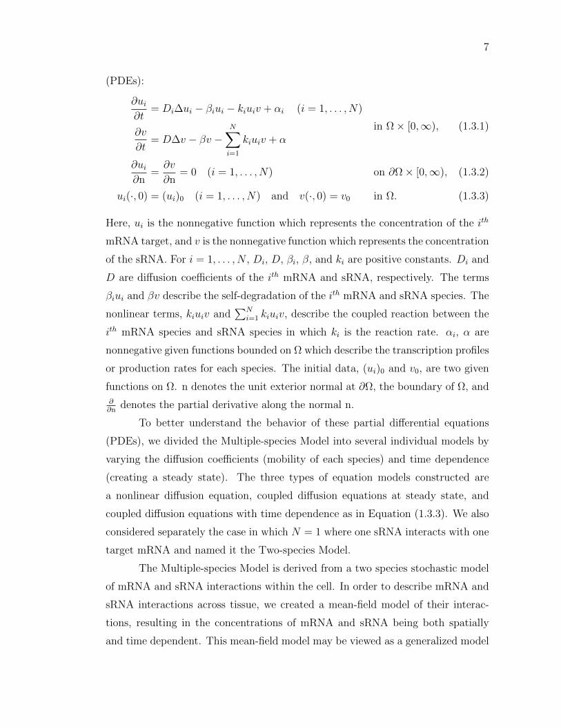
Let Ω be a bounded domain in R3, where the mRNA and sRNA interact.
Our model is a system of N + 1 reaction-diffusion partial differential equations
7
(PDEs):
∂ui∂t
= Di∆ui − βiui − kiuiv + αi (i = 1, . . . , N)
∂v
∂t= D∆v − βv −
N∑i=1
kiuiv + αin Ω× [0,∞), (1.3.1)
∂ui∂n
=∂v
∂n= 0 (i = 1, . . . , N) on ∂Ω× [0,∞), (1.3.2)
ui(·, 0) = (ui)0 (i = 1, . . . , N) and v(·, 0) = v0 in Ω. (1.3.3)
Here, ui is the nonnegative function which represents the concentration of the ith
mRNA target, and v is the nonnegative function which represents the concentration
of the sRNA. For i = 1, . . . , N , Di, D, βi, β, and ki are positive constants. Di and
D are diffusion coefficients of the ith mRNA and sRNA, respectively. The terms
βiui and βv describe the self-degradation of the ith mRNA and sRNA species. The
nonlinear terms, kiuiv and∑N
i=1 kiuiv, describe the coupled reaction between the
ith mRNA species and sRNA species in which ki is the reaction rate. αi, α are
nonnegative given functions bounded on Ω which describe the transcription profiles
or production rates for each species. The initial data, (ui)0 and v0, are two given
functions on Ω. n denotes the unit exterior normal at ∂Ω, the boundary of Ω, and
∂∂n
denotes the partial derivative along the normal n.
To better understand the behavior of these partial differential equations
(PDEs), we divided the Multiple-species Model into several individual models by
varying the diffusion coefficients (mobility of each species) and time dependence
(creating a steady state). The three types of equation models constructed are
a nonlinear diffusion equation, coupled diffusion equations at steady state, and
coupled diffusion equations with time dependence as in Equation (1.3.3). We also
considered separately the case in which N = 1 where one sRNA interacts with one
target mRNA and named it the Two-species Model.
The Multiple-species Model is derived from a two species stochastic model
of mRNA and sRNA interactions within the cell. In order to describe mRNA and
sRNA interactions across tissue, we created a mean-field model of their interac-
tions, resulting in the concentrations of mRNA and sRNA being both spatially
and time dependent. This mean-field model may be viewed as a generalized model

8
of chemical species across tissue that allows the parameters that are specific to
particular sRNA and mRNA interactions to be inputted easily.
Analysis of the Models
The analysis of our Multiple-species Model is divided into two types of sys-
tems: ordinary differential equation (ODE) systems and PDE systems. Analysis
of the ODE systems that are derived from our Multiple-Species Model shows that
the equilibrium solutions are stable subject to perturbations. The section on PDE
systems analysis illustrates the well-posedness of the three types of equations: a
single, nonlinear equation, coupled steady-state diffusion equations, and the time
dependent system of coupled equations. We also show using calculus of varia-
tions that the nonlinear equations associated with the Two-species Model and the
Multiple-species Model are unique.
Numerical Methods
In order to understand the behavior of our models numerically, we em-
ployed several numerical schemes. First, we discretized the space in which the
equations would lie by modifying the Finite Difference Method to account for our
Neumann boundary conditions. In addition, we created an alternating iteration
method to solve for our coupled PDEs. To approximate the time step, we em-
ployed the Forward Euler method and the Backward Euler method. Although the
Backward Euler scheme required more computations, we found that in our system,
the scheme converged faster than the Forward Euler scheme.
Computational Results
The numerical simulations for both the Two-species Model and the Multiple-
species Model show that when sRNA has a certain diffusion coefficient tolerance,
the concentration profile of mRNA displays a sharp interface between tissue with

9
high mRNA concentration and tissue with low mRNA concentration. That is, if
sRNA has some mobility across tissue, there is a sharp distinction between tissue
with high numbers of mRNA and tissue with low numbers of mRNA. When a
diffusion coefficient is added for the mRNA, the concentration profile of mRNA is
smoothed across the tissue. In other words, if mRNA has the ability to move across
tissue, the distinction recognized between tissue with high levels of mRNA and low
levels of mRNA is diminished. Another interest was how stable the interface be-
tween two species would be if small perturbations were introduced. We created a
perturbed sharp interface, and at steady state, the interface became sharp again.
That is, small fluctuations on a sharp interface will not change the shape of the
interface.
A sharpening of the concentration profile of mRNA may suggest a biological
regulation mechanism to minimize the number of cells where a gene is not strongly
expressed as on or off. Our model may give insight into how much mRNA and
sRNA molecules are needed for this type of regulation and how much diffusion (if
any) of each species leads to a working regulation mechanism. In some cancers for
which large concentrations of miRNA congregate in cells, the model may help us
predict how the concentrations effect gene expression across tissue.
Additionally, this numerical model also allows a simple input of specific
mRNA and sRNA characteristics such as production rates, independent degrada-
tion rates, and coupled degradation rates to see coupled behavior in tissue. In
addition, this model may be utilized to illustrate similar types of interactions be-
tween multiple chemical species.
Chapter 2
Mathematical Models
To construct the model of mRNA and sRNA interactions across tissue,
we first model the mRNA and sRNA interactions within the cell using a rate
diagram showing a network of states. From the diagram, we will create an ordinary
differential equation, the so-called master equation, that describes the change in
the mRNA and sRNA states at time t. This model of interactions within the cell
will be the basis for our partial differential equation (PDE) model of mRNA and
sRNA interactions across tissue.
2.1 Derivation of the Mean-field Model of Two
Species
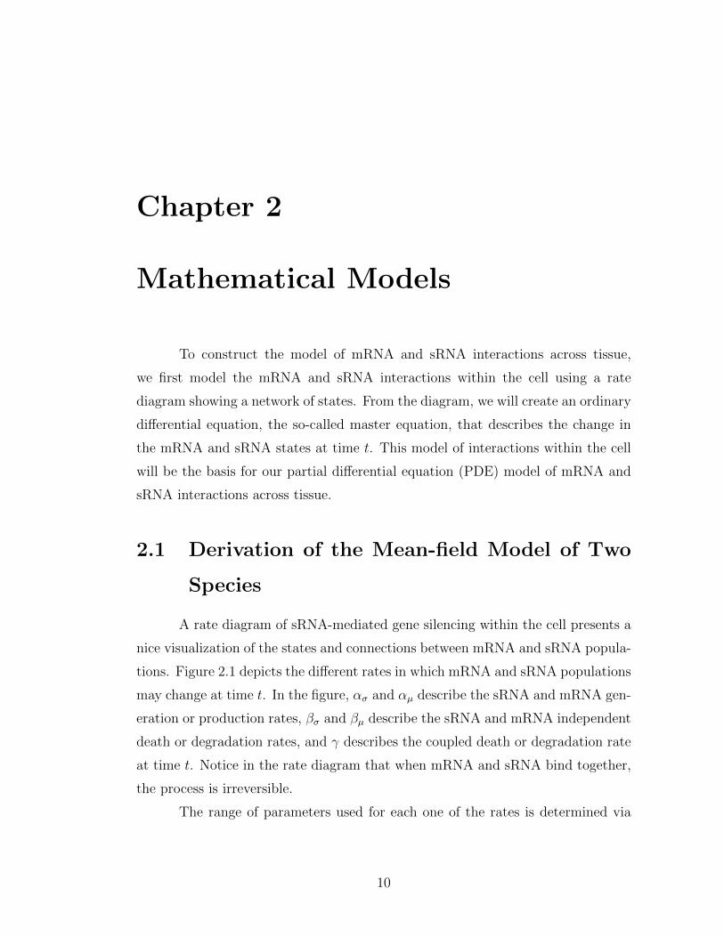
A rate diagram of sRNA-mediated gene silencing within the cell presents a
nice visualization of the states and connections between mRNA and sRNA popula-
tions. Figure 2.1 depicts the different rates in which mRNA and sRNA populations
may change at time t. In the figure, ασ and αµ describe the sRNA and mRNA gen-
eration or production rates, βσ and βµ describe the sRNA and mRNA independent
death or degradation rates, and γ describes the coupled death or degradation rate
at time t. Notice in the rate diagram that when mRNA and sRNA bind together,
the process is irreversible.
The range of parameters used for each one of the rates is determined via
10

11
experimental data [15]. For example, to find the coupled degradation rate, one
can inhibit transcription of mRNA and monitor its decay rate (total decay =
independent decay + coupled decay). If one knows the mRNA degradation rate
alone, then the coupled degradation rate is found. The parameters may change
based upon types of sRNA and the types of reactions occurring. Therefore, a range
of parameters will be explored to determine interaction responses.
sRNAmRNAαμ
ασ
βσ
γ
βμ
ø
ø
ø
Figure 2.1: Kinetic scheme of mRNA and sRNA concentrations. ασ and αµ rep-
resent the production rates of sRNA and mRNA, respectively. βσ and βµ represent
the independent degradation rates of sRNA and mRNA, respectively. γ represents
the couple degradation rate of sRNA and mRNA.
To construct our quantitative mathematical model from the diagram in
Figure 2.1, we first need to define some terms. Let (Mt)t≥0 and (St)t≥0 be two
continuous time processes with t ∈ [0,∞), where Mt represents the number of
mRNA in the cell at time t and St represents the number of sRNA in the cell at
time t. For notational convenience, let Nt = (Mt, St) represent the pair of RNA
populations in which the first number depicts the mRNA population at time t
and the second number depicts the sRNA population at time t. We will make the
following assumption regarding this time process:
Assumption. We assume that (Nt)t≥0 is a time-homogeneous continuous-time
Markov process with state space S with the following ordering:
S = ((0, 0), . . . , (m− 1, s− 1), (m− 1, s), (m, s− 1), (m, s), (m, s+ 1), . . .) .
12
Note that the number of mRNA and sRNA that can be created is bounded
above (by, say, the number of atoms in the universe). Because the number of both
mRNA and sRNA that can be created has a limit, the state space is finite.
Let P (t) be the time dependent (row) vector where
Pm,s(t) = P (Nt = (m, s)) = P (Mt = m,St = s).
Then,
P (t) = aP(t)
where a be the row vector indexed by S that represents the initial distribution of
the process and P(t) is the transition matrix.
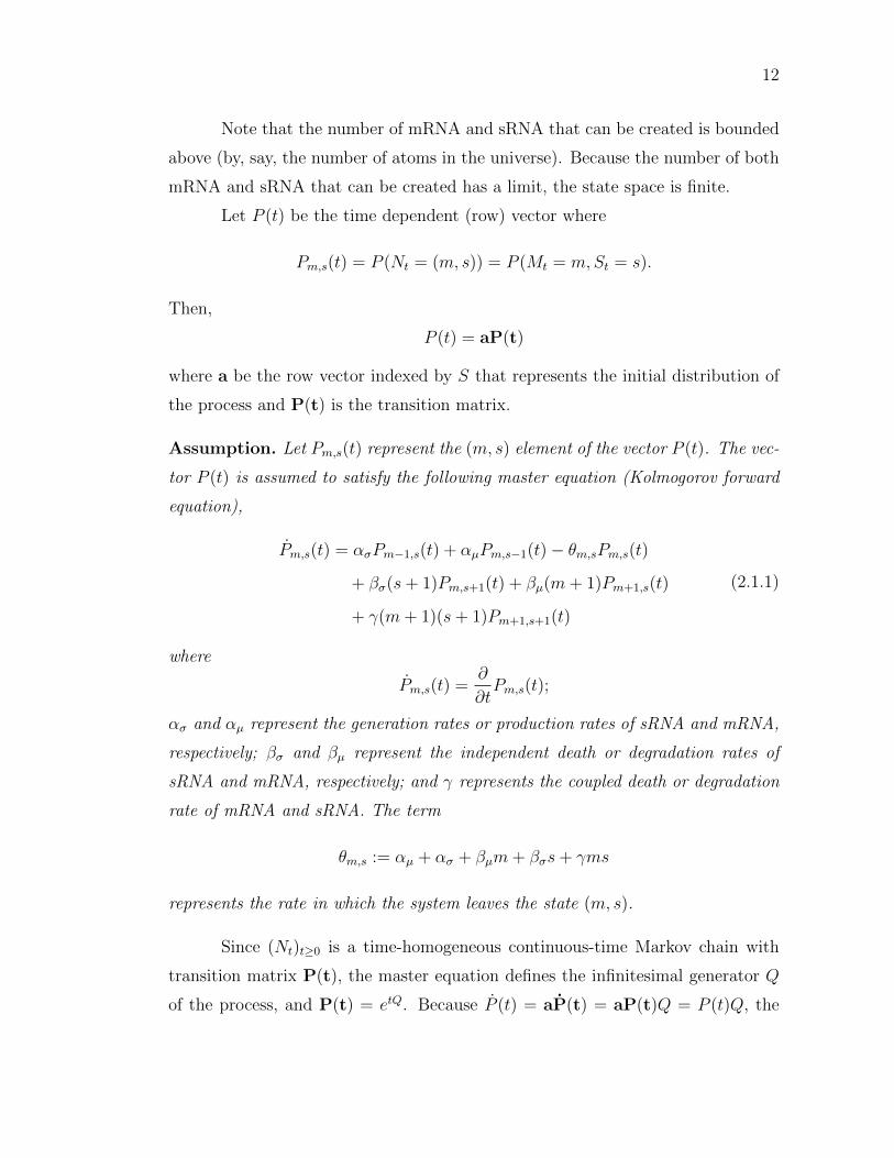
Assumption. Let Pm,s(t) represent the (m, s) element of the vector P (t). The vec-
tor P (t) is assumed to satisfy the following master equation (Kolmogorov forward
equation),
Pm,s(t) = ασPm−1,s(t) + αµPm,s−1(t)− θm,sPm,s(t)
+ βσ(s+ 1)Pm,s+1(t) + βµ(m+ 1)Pm+1,s(t)
+ γ(m+ 1)(s+ 1)Pm+1,s+1(t)
(2.1.1)
where
Pm,s(t) =∂
∂tPm,s(t);
ασ and αµ represent the generation rates or production rates of sRNA and mRNA,
respectively; βσ and βµ represent the independent death or degradation rates of
sRNA and mRNA, respectively; and γ represents the coupled death or degradation
rate of mRNA and sRNA. The term
θm,s := αµ + ασ + βµm+ βσs+ γms
represents the rate in which the system leaves the state (m, s).
Since (Nt)t≥0 is a time-homogeneous continuous-time Markov chain with
transition matrix P(t), the master equation defines the infinitesimal generator Q
of the process, and P(t) = etQ. Because P (t) = aP(t) = aP(t)Q = P (t)Q, the

13
master equation tells us that the column of Q corresponding to the state (m, s)
must be
column (m, s) of Q =
0...
0
ασ
αµ
−θm,sβσ(s+ 1)
βµ(m+ 1)
γ(m+ 1)(s+ 1)
0...
0
.
Notice that the diagonal elements of Q consist of −θ terms, and that the rows of
Q sum to 0. This means that Q is a Markov infinitesimal generator.
Proposition 2.1.1. Let ν ∈ RS = f | f : S → R. Then,
E [ν(Nt)] = P (t)ν.
On the left hand side, we view ν(Nt) as the composition of ν : S → R with the
random variable Nt. On the right hand side, we view P (t)ν as vector multiplication
between the row vector P (t) = aP(t) and ν which is identified as a column vector
indexed by S.
Proof. We have
E [ν(Nt)] =∑
(m,s)∈S
ν(m, s)P (Nt = (m, s)) =∑
(m,s)∈S
v(m, s)Pm,s(t) = P (t)ν.
Now, we have all of the tools to prove the following lemma that describes
the change in average mRNA and sRNA concentrations over time. This lemma
will also help us derive a mean-field model illustrating mRNA and sRNA molecule
movement within the cell and across tissue.

14
Lemma 2.1.1. For a random variable X, we denote the expectation of X by
〈X〉 = E [X]. Then, we have
∂
∂t〈Mt〉 = αµ − βµ 〈Mt〉 − γ 〈MtSt〉 (2.1.2)
∂
∂t〈St〉 = ασ − βσ 〈St〉 − γ 〈MtSt〉 . (2.1.3)
Proof. Define [A]m,s to be the (m, s) entry of the matrix A. Let πµ and πσ be the
projection maps from S → R given by πµ(m, s) = m and πσ(m, s) = s. Then,
〈Mt〉 = E [πµ(Nt)] and 〈St〉 = E [πσ(Nt)]. Using Proposition 2.1.1 with ν = πµ and
using the properties of Q, we get
∂
∂tE [πµ(Nt)] =
∂
∂tP (t)πµ = [P (t)Q] πµ
=∑
(m,s)∈S
πµ(m, s) [P (t)Q]m,s
=∑
(m,s)∈S
m [P (t)Q]m,s
By recalling that [P (t)Q]m,s = Pm,s(t) and using our master equation (Equa-
tion (2.1.1)), the last equality becomes∑(m,s)∈S
m [P (t)Q]m,s =∑
(m,s)∈S
m
(αµPm−1,s(t) + ασPm,s−1(t)− θm,sPm,s(t)
+ βσ(s+ 1)Pm,s+1(t) + βµ(m+ 1)Pm+1,s(t)
+ γ(m+ 1)(s+ 1)Pm+1,s+1(t)
).
Since we are summing over a finite set S, we interchange the sum and the differ-
ential operator to get the following:

15
∂
∂t
∑(m,s)∈S
mPm,s(t) = αµ
∑(m,s)∈S
mPm−1,s(t)−∑
(m,s)∈S
mPm,s(t)
+ ασ
∑(m,s)∈S
mPm,s−1(t)−∑
(m,s)∈S
mPm,s(t)
+ βµ
∑(m,s)∈S
m(m+ 1)Pm+1,s(t)−∑
(m,s)∈S
m2Pm,s(t)
+ βσ
∑(m,s)∈S
m(s+ 1)Pm,s+1(t)−∑
(m,s)∈S
msPm,s(t)
+ γ
∑(m,s)∈S
m(m+ 1)(s+ 1)Pm+1,s+1(t)
− γ∑
(m,s)∈S
m2sPm,s(t)
∂
∂t
∑(m,s)∈S
mPm,s(t) = αµ
∑(m−1,s)∈S
(m+ 1)Pm,s(t)−∑
(m,s)∈S
mPm,s(t)
+ ασ
∑(m,s−1)∈S
mPm,s(t)−∑
(m,s)∈S
mPm,s(t)
+ βµ
∑(m+1,s)∈S
(m− 1)mPm,s(t)−∑
(m,s)∈S
m2Pm,s(t)
+ βσ
∑(m,s+1)∈S
msPm,s(t)−∑
(m,s)∈S
msPm,s(t)
+ γ
∑(m+1,s+1)∈S
(m− 1)msPm,s(t)−∑
(m,s)∈S
m2sPm,s(t)

16
∂
∂t
∑(m,s)∈S
mPm,s(t) = αµ
∑(m,s)∈S
(m+ 1)Pm,s(t)−∑
(m,s)∈S
mPm,s(t)
+ ασ
∑(m,s)∈S
mPm,s(t)−∑
(m,s)∈S
mPm,s(t)
+ βµ
∑(m,s)∈S
(m− 1)mPm,s(t)−∑
(m,s)∈S
m2Pm,s(t)
+ βσ
∑(m,s)∈S
msPm,s(t)−∑
(m,s)∈S
msPm,s(t)
+ γ
∑(m,s)∈S
(m− 1)msPm,s(t)−∑
(m,s)∈S
m2sPm,s(t)
∂
∂t
∑(m,s)∈S
mPm,s(t) = αµ∑
(m,s)∈S
Pm,s(t)
+ βµ
∑(m,s)∈S
(m2 −m)Pm,s(t)−∑
(m,s)∈S
m2Pm,s(t)
+ γ
∑(m,s)∈S
(m2s−ms)Pm,s(t)−∑
(m,s)∈S
m2sPm,s(t)
And,
∂
∂t
∑(m,s)∈S
mPm,s(t) = αµ − βµ∑
(m,s)∈S
mPm,s(t)− γ∑
(m,s)∈S
msPm,s(t).
Since∑
(m,s)∈SmPm,s(t) = 〈Mt〉,
∂
∂t〈Mt〉 = αµ − βµ 〈Mt〉 − γ 〈MtSt〉 .
Mimicking the above process for 〈St〉 = E [πσ(Nt)] = P (t)πσ using the master
equation (Equation (2.1.1)), we have
∂
∂t〈St〉 = ασ − βσ 〈St〉 − γ 〈MtSt〉 .

17
Because we are looking for insight into the concentrations of mRNA and
sRNA molecules not just inside cells, but concentrations at the tissue level, we
modify Equations (2.1.2) and (2.1.3) using mean-field theory to examine the be-
havior of many mRNA molecules at once. The mean-field assumption is that
〈MtSt〉 = 〈Mt〉 〈St〉 . (2.1.4)
Therefore, by integrating this assumption into Equations (2.1.2) and (2.1.3), we
have the following coupled differential equations:
Let u(t) = 〈Mt〉 and v(t) = 〈St〉.∂u
∂t= αµ − βµu− γuv,
∂v
∂t= ασ − βσv − γuv .
Although the above equations describe binding of mRNA and sRNA within
a cell across tissue, they do not describe the process of sRNA movement between
cells documented in cell differentiation and development [28, 31]. To describe this
movement, we must add a diffusion process with an appropriate diffusion coefficient
Dσ to the sRNA equation [14]. We have the following equations:
∂u
∂t= αµ − βµu− γuv, (2.1.5)
∂v
∂t= ασ − βσv − γuv +Dσ∆v . (2.1.6)
Furthermore, we account for the intercellular macromolecule movement of mRNA
such as with exosome-mediated transfer [30] by adding mRNA movement across
tissue. We model this behavior by adding a diffusion processes with an appropriate
diffusion coefficient Dµ to Equation (2.1.5) to form the following coupled equations:
∂u
∂t= αµ − βµu− γuv +Dµ∆u, (2.1.7)
∂v
∂t= ασ − βσv − γuv +Dσ∆v. (2.1.8)
The coupled reaction-diffusion equations above illustrate mRNA and sRNA
concentration levels across tissue developed from the stochastic master equation
(2.1.1). These equations will transform into two types of models: two-species
models and multiple-species models.

18
2.2 Two-species Models in Multiple Dimensions
A dynamic model allowing for both mRNA and sRNA to move inside and
outside of the cell as well as across tissue in a multiple-dimension model would
bring accuracy to the behavior of RNA molecules across tissue. By adapting
Equations (2.1.7) and (2.1.8) and adding some reasonable boundary conditions, we
create coupled reaction-diffusion equations for a multiple dimensional environment.
Let Ω be a bounded domain in R3 where the mRNA and sRNA interact.
Let u = u(x, t) and v = v(x, t) denote the concentrations of mRNA and sRNA,
respectively, at a spatial point x = (x1, x2, x3) ∈ Ω at time t. The following
reaction-diffusion equations model the concentrations with specified boundary and
initial conditions:
∂u
∂t= D1∆u− β1u− k1uv + α1
∂v
∂t= D∆v − βv − k1uv + α
in Ω× [0,∞), (2.2.1)
∂u
∂n=∂v
∂n= 0 on ∂Ω× [0,∞), (2.2.2)
u(·, 0) = u0 and v(·, 0) = v0 in Ω. (2.2.3)
Here, u is the nonnegative function which represents the concentration of the
mRNA, and v is the nonnegative function which represents the concentration of
the sRNA. D, D1, β, β1, k1, and k1 are positive constants. D1 and D are diffusion
coefficients of mRNA and sRNA, respectively. The terms β1u and βv describe the
self-degradation of the two species mRNA and sRNA, respectively. The nonlinear
terms, k1uv and k1uv, describe the coupled reaction between the two species in
which k1 and k1 are the reaction rates. α1 and α are nonnegative given functions
defined on Ω which describe the transcription profiles or production rates for each
species. The initial data, u0 and v0, are two given functions on Ω. n denotes
the unit exterior normal at ∂Ω, the boundary of Ω, and ∂∂n
denotes the partial
derivative along the normal n.
We consider three different cases of the above model, and name the cor-
responding models Two-species Model I, Two-species Model, II, and Two-species
Model III.

19
Two-species Model I: A single, nonlinear PDE
First, we let mRNA diffuse very slowly with D1 = 0 and D > 0. Moreover, we as-
sume the concentration of mRNA reaches a steady-state in which the time deriva-
tive of u vanishes. The time independent equation for u from Equation (2.2.1)
becomes
u =α1
β1 + k1vin Ω.
Thus, the steady-state concentration v = v(x) of sRNA is governed by the following
nonlinear, diffusion equation and boundary condition:
D∆v − βv − k1α1v
β1 + k1v+ α = 0 in Ω, (2.2.4)
∂v
∂n= 0 on ∂Ω. (2.2.5)
Two-species Model II: Coupled, steady-state diffusion equations
We consider the steady-state concentrations of both species with D1, D > 0 and
study the following coupled steady-state diffusion equations:
D1∆u− β1u− k1uv + α1 = 0
D∆v − βv − k1uv + α = 0in Ω, (2.2.6)
∂u
∂n=∂v
∂n= 0 on ∂Ω. (2.2.7)
Two-species Model III: Coupled, time-dependent diffusion equations
This model is our original coupled reaction-diffusion Equations (2.2.1)–(2.2.3):
∂u
∂t= D1∆u− β1u− k1uv + α1
∂v
∂t= D∆v − βv − k1uv + α
in Ω× [0,∞),
∂u
∂n=∂v
∂n= 0 on ∂Ω× [0,∞),
u(·, 0) = u0 and v(·, 0) = v0 in Ω.
20
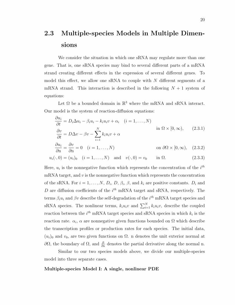
2.3 Multiple-species Models in Multiple Dimen-
sions
We consider the situation in which one sRNA may regulate more than one
gene. That is, one sRNA species may bind to several different parts of a mRNA
strand creating different effects in the expression of several different genes. To
model this effect, we allow one sRNA to couple with N different segments of a
mRNA strand. This interaction is described in the following N + 1 system of
equations:
Let Ω be a bounded domain in R3 where the mRNA and sRNA interact.
Our model is the system of reaction-diffusion equations:
∂ui∂t
= Di∆ui − βiui − kiuiv + αi (i = 1, . . . , N)
∂v
∂t= D∆v − βv −
N∑i=1
kiuiv + αin Ω× [0,∞), (2.3.1)
∂ui∂n
=∂v
∂n= 0 (i = 1, . . . , N) on ∂Ω× [0,∞), (2.3.2)
ui(·, 0) = (ui)0 (i = 1, . . . , N) and v(·, 0) = v0 in Ω. (2.3.3)
Here, ui is the nonnegative function which represents the concentration of the ith
mRNA target, and v is the nonnegative function which represents the concentration
of the sRNA. For i = 1, . . . , N , Di, D, βi, β, and ki are positive constants. Di and
D are diffusion coefficients of the ith mRNA target and sRNA, respectively. The
terms βiui and βv describe the self-degradation of the ith mRNA target species and
sRNA species. The nonlinear terms, kiuiv and∑N
i=1 kiuiv, describe the coupled
reaction between the ith mRNA target species and sRNA species in which ki is the
reaction rate. αi, α are nonnegative given functions bounded on Ω which describe
the transcription profiles or production rates for each species. The initial data,
(ui)0 and v0, are two given functions on Ω. n denotes the unit exterior normal at
∂Ω, the boundary of Ω, and ∂∂n
denotes the partial derivative along the normal n.
Similar to our two species models above, we divide our multiple-species
model into three separate cases.
Multiple-species Model I: A single, nonlinear PDE

21
As with Model I, we suppose ith mRNA target diffuses very slowly. We let Di = 0
and D > 0 to have the following nonlinear PDE at steady state:
D∆v − βv −N∑i=1
αikiv
βi + kiv+ α = 0 in Ω, (2.3.4)
∂v
∂n= 0 on ∂Ω. (2.3.5)
Multiple-species Model II: Coupled, steady-state diffusion equations
We consider the steady-state concentrations of all species with Di, D > 0 and
study the following coupled steady-state diffusion equations:
Di∆ui − βiui − kiuiv + αi = 0 (i = 1, . . . , N)
D∆v − βv −N∑i=1
kiuiv + α = 0in Ω, (2.3.6)
∂ui∂n
=∂v
∂n= 0 (i = 1, . . . , N) on ∂Ω. (2.3.7)
Multiple-species Model III: Coupled, time-dependent diffusion equa-
tions
This model is the coupled reaction-diffusion Equations (2.3.1)–(2.3.3):
∂ui∂t
= Di∆ui − βiui − kiuiv + αi (i = 1, . . . , N)
∂v
∂t= D∆v − βv −
N∑i=1
kiuiv + αin Ω× [0,∞),
∂ui∂n
=∂v
∂n= 0 (i = 1, . . . , N) on ∂Ω× [0,∞),
ui(·, 0) = (ui)0 (i = 1, . . . , N) and v(·, 0) = v0 in Ω.
Chapter 3
Mathematical Analysis of the
Models
The mathematical analysis of the Two-species Model and the Multiple-
species Model is divided into two sections: analysis dealing with ordinary differen-
tial equations (ODEs) derived from our models and analysis of PDEs associated
with our models. The ODE section asks if the equilibrium solutions are stable
subject to perturbations. The PDE section addresses existence and uniqueness of
the models derived from the Two-species Model and the Multiple-species Model.
3.1 Ordinary Differential Equations Analysis
First, we neglect the spatial dependence of the Multiple-species Model sys-
tem of equations and study the resulting ODEs. We will then solve for steady
state solutions of the ODE system and linearize a system around such a steady
state solution. The eigenvalues of the associated matrix to the linearized system
determines stability.
22
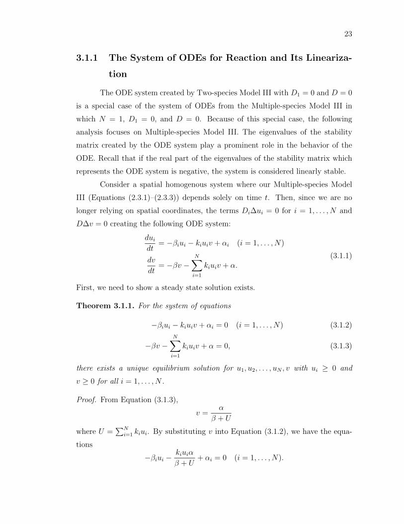
23
3.1.1 The System of ODEs for Reaction and Its Lineariza-
tion
The ODE system created by Two-species Model III with D1 = 0 and D = 0
is a special case of the system of ODEs from the Multiple-species Model III in
which N = 1, D1 = 0, and D = 0. Because of this special case, the following
analysis focuses on Multiple-species Model III. The eigenvalues of the stability
matrix created by the ODE system play a prominent role in the behavior of the
ODE. Recall that if the real part of the eigenvalues of the stability matrix which
represents the ODE system is negative, the system is considered linearly stable.
Consider a spatial homogenous system where our Multiple-species Model
III (Equations (2.3.1)–(2.3.3)) depends solely on time t. Then, since we are no
longer relying on spatial coordinates, the terms Di∆ui = 0 for i = 1, . . . , N and
D∆v = 0 creating the following ODE system:
duidt
= −βiui − kiuiv + αi (i = 1, . . . , N)
dv
dt= −βv −
N∑i=1
kiuiv + α.(3.1.1)
First, we need to show a steady state solution exists.
Theorem 3.1.1. For the system of equations
−βiui − kiuiv + αi = 0 (i = 1, . . . , N) (3.1.2)
−βv −N∑i=1
kiuiv + α = 0, (3.1.3)
there exists a unique equilibrium solution for u1, u2, . . . , uN , v with ui ≥ 0 and
v ≥ 0 for all i = 1, . . . , N .
Proof. From Equation (3.1.3),
v =α
β + U
where U =∑N
i=1 kiui. By substituting v into Equation (3.1.2), we have the equa-
tions
−βiui −kiuiα
β + U+ αi = 0 (i = 1, . . . , N).

24
Then,
ui =αi
βi + kiα (β + U)−1 (i = 1, . . . , N),
and
U =N∑i=1
kiui =N∑i=1
kiαi
βi + kiα (β + U)−1 .
Now, we want to show that the equation
U −N∑i=1
kiαi
βi + kiα (β + U)−1 = 0
has a unique solution. Let the function g : [0,∞)→ R be defined by
g(s) = s−N∑i=1
kiαi
βi + kiα (β + s)−1 , (3.1.4)
and recall that βi, β, and ki are positive constants and αi and α are nonnegative
functions. g is smooth in our domain [0,∞). Since
g(0) = −N∑i=1
kiαi
βi + kiα (β)−1 ≤ 0
and the lims→∞ g(s) = +∞, there exists a s ∈ [0,∞) such that g(s) = 0. That is,
there exists a U ∈ [0,∞) such that g(U) = 0. Then,
v =α
β + U,
and v has a solution. Similarly,
ui =αi
βi + kiv(i = 1, . . . , N),
and ui has a solution for all i. To find the behavior of the possible root(s), we first
look at the derivatives of g. The first derivative of g is
g′(s) = 1−N∑i=1
k2i αiα
(βi (β + s) + kiα)2 ,

25
and the second derivative of g is
g′′(s) = 2αN∑i=1
k2i αiβi
(βi (β + s) + kiα)3 ≥ 0.
Notice that g′′(s) = 0 on [0,∞) only when α = 0 or αi = 0 for all i. In both
cases, g(s) is then a linear equation with only one solution, and g(s) has a unique
solution U such that g(U) = 0.
Suppose g′(s) ≥ 0 on [0,∞). Since g is convex and concave up (g′′(s) > 0),
g(U) = 0 is the unique minimizer. Suppose, on the other hand, g′(s) < 0. Then, g
attains its minimum in [0, U ] at some s0 ∈ (0, U) where g′(s0) = 0. In the interval
[0, s0), g′(s) < 0 and g(s) < 0. In the interval (s0,∞), g′(s) > 0 and g′′(s) > 0.
Hence, g(s) = 0 in only one place. That is, g(s) has at most one root. This proves
uniqueness.
Define u0i and v0 to be the solutions to the coupled equations (3.1.1). That
is,
−βiu0i − kiu0iv0 + αi = 0 (i = 1, . . . , N)
−βv0 −N∑i=1
kiu0iv0 + α = 0.
For ε > 0, define the equations ui(t) and v(t) by
ui(t) = u0i + εu1i(t) +O(ε2)
(i = 1, . . . , N) (3.1.5)
v(t) = v0 + εv1(t) +O(ε2). (3.1.6)
By rewriting Equations (3.1.5) and (3.1.6), we have the following equations de-
scribing our ODE:
εu1i = ui − u0i +O(ε2) (i = 1, . . . , N) (3.1.7)
εv1 = v − v0 +O(ε2). (3.1.8)
For each i = 1, . . . , N , we take the derivative of both sides of Equation (3.1.7) with

26
respect to t,
εdu1i
dt=duidt− du0i
dt+O(ε2)
= (−βiui − kiuiv + α1)− (−βiu0i − kiu0iv0 + α1) +O(ε2)
= −βi(ui − u0i)− ki(uiv − u0iv0) +O(ε2)
= −βi(ui − u0i)− ki((ui − u0i)(v − v0) + uiv0 + u0iv − 2u0iv0) +O(ε2)
= −βi(ui − u0i)− ki((ui − u0i)(v − v0) + v0(ui − u0i) + u0i(v − v0))
+O(ε2)
= −βi(ui − u0i)− kiv0(ui − u0i)− kiu0i(v − v0)− ki(ui − u0i)(v − v0)
+O(ε2)
= −(βi + kiv0)(ui − u0i)− kiu0i(v − v0)− ki(ui − u0i)(v − v0) +O(ε2)
= −ε(βi + kiv0)u1i − εkiu0iv1 +O(ε2).
Then, we havedu1i
dt= −(βi + kiv0)u1i − kiu0iv1 +O(ε).
Similarly, by taking the derivative of Equation (3.1.8),
εdv1
dt=dv
dt− dv0
dt+O(ε2)
= (−βv −N∑i=1
kiuiv + α)− (−βv0 −N∑i=1
kiu0iv0 + α) +O(ε2)
= −β(v − v0)−N∑i=1
ki(uiv − u0iv0) +O(ε2)
= −β(v − v0)−N∑i=1
ki((ui − u0i)(v − v0) + uiv0 + u0iv − 2u0iv0) +O(ε2)
= −β(v − v0)−N∑i=1
ki [u0i(v − v0) + (ui − u0i)v0 + (ui − u0i)(v − v0)]
+O(ε2)
= −(β +N∑i=1
kiu0i)(v − v0)−N∑i=1
ki [(ui − u0i)v0 + (ui − u0i)(v − v0)]
+O(ε2)

27
= −ε(β +N∑i=1
kiu0i)v1 − εN∑i=1
kiv0u1i +O(ε2).
And, we have
dv1
dt= −
(β +
N∑i=1
kiu0i
)v1 −
N∑i=1
kiv0u1i +O(ε).
For i = 1, . . . , N , we have the coupled system of N + 1 equations
du1i
dt= −(βi + kiv0)u1i − kiu0iv1 +O(ε)
dv1
dt= −
(β +
N∑i=1
kiu0i
)v1 −
N∑i=1
kiv0u1i +O(ε).
Define w =
u11
u12
...
u1N
v1
. We obtain the linearized system
dw
dt= Mw,
where
M =
−(β1 + k1v0) 0 . . . 0 −k1u01
0 −(β2 + k2v0) . . . 0 −k2u02
......
. . ....
0 0 −(βN + kNv0) −kNu0N
−k1v0 −k2v0 . . . −kNv0 −(β +∑N
i=1 kiu0i)
(3.1.9)
We call this matrix the stability matrix. If the real parts of the eigenvalues of M
are negative, the system is considered to be linearly stable.
3.1.2 Linear Stability
To show the real parts of the eigenvalues of M are negative, we will show
that the diagonal dominance and the negative diagonal elements of M cause each

28
eigenvalue of M to be contained in a Gershgorin disc lying in the left-half plane.
Since <(λ(M)) < 0, the ODE is stable. We start by showing the column diagonal
dominance of M .
Proposition 3.1.1. Assume β, βi, ki > 0 and u0i , v0 ≥ 0 for all i = 1, . . . , N .
Then, the matrix M from (3.1.9) is strictly column diagonally dominant.
Proof. M = [mij] is said to be strictly column diagonally dominant if for all
j = 1, . . . , N + 1,
|mjj| >N+1∑i=1i 6=j
|mij| .
For columns j = 1, . . . , N ,
|mjj| = |βj + kjv0| > |kjv0| =N+1∑i=1i 6=j
|mij| .
For j = N + 1,
|mN+1,N+1| =
∣∣∣∣∣β +N∑i=1
kiu0i
∣∣∣∣∣ >∣∣∣∣∣N∑i=1
kiu0i
∣∣∣∣∣ =N∑i=1
|mi,N+1| .
Hence, M is strictly column diagonally dominant.
Since M is strictly column diagonally dominant, MH is row diagonally
dominant with corresponding eigenvalues λ(M) = λ(MH). We will now show that
the eigenvalues of MH have negative real part by the following theorem.
Theorem 3.1.2. Let A = [aij] ∈ Rn×n be strictly row diagonally dominant. Then,
if all main diagonal entries of A are negative, then all the eignenvalues of A have
negative real part.
Proof. Let A = [aij] be strictly row diagonally dominant with all negative main
diagonal entries. Let λ be an eigenvalue of A with the corresponding eigenvector
x. For x = [xi] 6= 0, there exists a p such that |xp| ≥ |xi| for all i = 1, . . . , n, and
|xp| 6= 0. Since Ax = λx,
λxp = [λx]p = [Ax]p =n∑i=1
apixi = appxp +n∑i=1i 6=j
apixi,

29
and
(λ− app)xp =n∑i=1i 6=j
apixi.
Hence,
|λ− app| |xp| = |(λ− app)xp| =
∣∣∣∣∣∣∣n∑i=1i 6=j
apixi
∣∣∣∣∣∣∣ ≤n∑i=1i 6=j
|api| |xi| ≤ |xp|n∑i=1i 6=j
|api| .
Since A is row diagonally dominant,
|λ− app| ≤n∑i=1i 6=j
|api| < |app| .
Therefore, λ ∈ z : |z − app| < |app|. That is, λ exists in a disk in the complex
plane centered at app ∈ R− of radius less than |app|. Thus, <(λ) exists in the
left-half plane.
Since M is strictly column diagonally dominant, MH is strictly row diago-
nally dominant. By Theorem 3.1.2, the eigenvalues of MH have all negative real
part. Since λ(MH) = λ(M), the real part of the eigenvalues of M all have negative
real part, and the system is asymptotically stable.
3.2 Partial Differential Equations Analysis
The following section focuses on the analysis of the PDEs derived from the
Two-species Model and the Multiple-species Model. In particular, we find that
the solutions to the Two-species Model I and the solutions to the Multiple-species
Model I exist and are unique. We also find that a solution to Two-species Model
II exists, but may not necessarily be unique.
3.2.1 Well-posedness of Two-species Model I
We show that Two-species Model I has a unique solution in Ω.

30
Theorem 3.2.1. Assume Ω has a Lipschitz-continuous boundary. The boundary-
value problem
D∆v − βv − k1α1v
β1 + k1v+ α = 0 in Ω, (3.2.1)
∂v
∂n= 0 on ∂Ω. (3.2.2)
(Two-species Model I, Section 2.2, Equations 2.2.4 and 2.2.5) has a unique solution
v ∈ H1(Ω) such that v ≥ 0, and v is smooth in Ω.
Proof. Define J : H1(Ω)→ R ∪ ±∞ by
J [v] =
∫Ω
D
2|∇v|2 +
β
2v2 +
k1α1β1
k21
[k1
β1
v − ln
(1 +
k1
β1
v
)]− αv
dx.
Define ln s = −∞ for any s ≤ 0. Notice that the function
g(s) = s− ln(1 + s) (−1 < s <∞)
is strictly convex and reaches its minimum g(0) = 0. Thus, there exists constants
C1 > 0 and C2 ≥ 0 such that
J [v] ≥ C1‖v‖2H1(Ω) − C2 ∀v ∈ H1(Ω). (3.2.3)
If we denote θ = infv∈H1(Ω) J [v], then θ is finite. Let vj ∈ H1(Ω) (j = 1, 2, . . . ) be
such that J [vj]→ 0 as j →∞. It follows from Equation (3.2.3) that, passing to a
subsequence if necessary, vj∞j=1 converges to some v ∈ H1(Ω), weakly in H1(Ω),
strongly in L2(Ω), and a.e. in Ω. Since the function g(s) ≥ 0 for all s ∈ (−1,∞),
Fatou’s Lemma implies that
lim infj→∞
∫Ω
[k1
β1
vj − ln
(1 +
k1
β1
vj
)]dx ≥
∫Ω
[k1
β1
v − ln
(1 +
k1
β1
v
)]dx.
The weak convergence in H1(Ω) and strong convergence in L2(Ω) of vj∞j=1 to v
now imply that
lim infj→∞
J [vj] ≥ J [v].
Hence, J [v] = θ. The strict convexity of J implies that v ∈ H1(Ω) is the unique
minimizer of J : H1(Ω)→ R ∪ +∞.

31
Now we will show that v ≥ 0 a.e. in Ω. By the uniqueness of the minimizer
of J over H1(Ω), it suffices to show that |v| ∈ H1(Ω) is also a minimizer. Notice
that |∇|v| | ≤ |∇v| in Ω. Since α is nonnegative in Ω, we have −α|v| ≤ −αv a.e.
in Ω. Notice that for any s ∈ (−1, 0]
g(|s|)− g(s) = |s| − ln(1 + |s|)− [s− ln(1 + s)] = −2s+ ln
(1 + s
1− s
).
It is easy to verify that this continuous function of s has a positive derivative in
(−1, 0) and is equal to 0 at s = 0. Therefore, g(|s|) ≥ g(s) for s ∈ (−1, 0). Applying
this to the case, s = k1v(x)/β1 ∈ (−1, 0] for some some x ∈ Ω. Therefore, we obtain
that J [|v|] ≥ J [v]. Hence v ≥ 0.
It now follows that
d
dt
∣∣∣∣t=0
∫Ω
ln
(1 +
k1
β1
(v + tw)
)dx =
(k1/β1)w
1 + (k1/β1)v∀w ∈ H1(Ω).
Since v minimizes J over H1(Ω), we have
d
dt
∣∣∣∣t=0
J [v + tw] = 0 ∀w ∈ H1(Ω).
Standard calculations then imply that v ∈ H1(Ω) is a weak solution to Equa-
tion (2.2.4) and Equation (2.2.5). The smoothness of v inside Ω follows from a
standard bootstrapping technique.
3.2.2 Well-posedness of Multiple-species Model I
We will show that Multiple-species Model I is unique.
Theorem 3.2.2. Assume Ω has a Lipschitz-continuous boundary. The equation
D∆v − βv −N∑i=1
kiαiv
βi + kiv+ α = 0 in Ω, (3.2.4)
∂v
∂n= 0 on ∂Ω,
has a unique solution v ∈ H1(Ω) such that v ≥ 0, and v is smooth in Ω.
Proof. Follow the proof of Theorem 3.2.1 with the functional
J [v] =
∫Ω
D
2|∇v|2 +
β
2v2 +
N∑i=1
αiβiki
[kiβiv − ln
(1 +
kiβiv
)]− αv
dx.
32
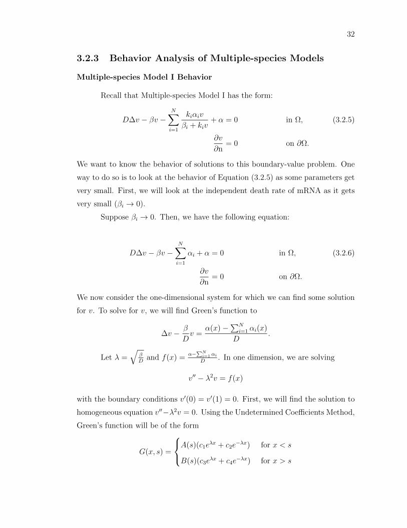
3.2.3 Behavior Analysis of Multiple-species Models
Multiple-species Model I Behavior
Recall that Multiple-species Model I has the form:
D∆v − βv −N∑i=1
kiαiv
βi + kiv+ α = 0 in Ω, (3.2.5)
∂v
∂n= 0 on ∂Ω.
We want to know the behavior of solutions to this boundary-value problem. One
way to do so is to look at the behavior of Equation (3.2.5) as some parameters get
very small. First, we will look at the independent death rate of mRNA as it gets
very small (βi → 0).
Suppose βi → 0. Then, we have the following equation:
D∆v − βv −N∑i=1
αi + α = 0 in Ω, (3.2.6)
∂v
∂n= 0 on ∂Ω.
We now consider the one-dimensional system for which we can find some solution
for v. To solve for v, we will find Green’s function to
∆v − β
Dv =
α(x)−∑N
i=1 αi(x)
D.
Let λ =√
βD
and f(x) =α−
∑Ni=1 αiD
. In one dimension, we are solving
v′′ − λ2v = f(x)
with the boundary conditions v′(0) = v′(1) = 0. First, we will find the solution to
homogeneous equation v′′−λ2v = 0. Using the Undetermined Coefficients Method,
Green’s function will be of the form
G(x, s) =
A(s)(c1eλx + c2e
−λx) for x < s
B(s)(c3eλx + c4e
−λx) for x > s

33
for constants c1, c2, c3, c4 and functions A(s) 6= 0 and B(s) 6= 0. We can solve for
these variables using the conditions which G(x, s) must satisfy such as boundary
conditions, continuity at x and s, and the derivative “jump” when x → s. For
x < s,
G′(x, s) = A(s)(c1λeλx − c2λe
−λx)
G′(0, s) = A(s)(c1λ− c2λ)
c2 = c1.
For x > s,
G′(x, s) = B(s)(c3λeλx − c4λe
−λx)
G′(1, s) = B(s)(c3λeλ − c4λe
−λ)
c4e−λ = c3e
λ
c4 = c3e2λ.
Then,
G(x, s) =
A(s)(c1eλx + c1e
−λx) for x < s
B(s)(c3eλx + c3e
2λ−λx) for x > s.
From continuity at x = s,
A(s)(c1eλs + c1e
−λs) = B(s)(c3eλs + c3e
2λ−λs).
From the derivative “jump” where G′(s+, s)−G′(s−, s) = 1,
B(s)(λc3eλs − λc3e
2λ−λs)− A(s)(c1λeλs − c1λe
−λs) = 1.
Together,A(s)(c1λeλs + c1λe
−λs)−B(s)(c3λeλs + c3λe
2λ−λs) = 0
−A(s)(c1λeλs − c1λe
−λs) +B(s)(c3λeλs − c3λe
2λ−λs) = 1,
and so,
2A(s)c1λe−λs − 2B(s)c3λe
2λ−λs = 1.

34
Then,
A(s)c1 =1
2λeλs +B(s)c3e
2λ.
By substitution,(1
2eλs + λB(s)c3e
2λ
)(eλs + e−λs
)−B(s)c3λe
λs(1 + e2λ−2λs
)= 0
1
2
(e2λs + 1
)+ λB(s)c3e
2λ+λs + λB(s)c3e2λ−λs − λB(s)c3e
λs(1 + e2λ−2λs
)= 0
1
2
(e2λs + 1
)+ λB(s)c3e
2λ+λs − λB(s)c3eλs = 0
1
2
(e2λs + 1
)+ λB(s)c3e
λs(e2λ − 1
)= 0
Solving for c3,
λB(s)c3eλs(e2λ − 1
)= −1
2
(e2λs + 1
)B(s)c3 = −1
λ
(e2λs + 1
2eλs (e2λ − 1)
)Substituting A(s)c1 and B(s)c3 into G(x, s), we have
G(x, s) =
(
12λeλs − 1
λ
(e2λs+1
2eλs(e2λ−1)
)e2λ
)(eλx + e−λx) for x < s
− 1λ
(e2λs+1
2eλs(e2λ−1)
)(eλx + e2λ−λx) for x > s.
By collecting terms, we have
G(x, s) =
(e2λs(e2λ−1)−(e2λs+1)e2λ
2λeλs(e2λ−1)
)(eλx + e−λx
)for x < s
−(
e2λs+1
2λeλs(e2λ−1)
)(eλx + e2λ−λx) for x > s.
Further consolidation,
G(x, s) =
(e2λ+2λs−e2λs−e2λs+2λ−e2λ
2λeλs(e2λ−1)
)(eλx + e−λx
)for x < s
−(
e2λs+1
2λeλs(e2λ−1)
)(eλx + e2λ−λx) for x > s.

35
G(x, s) =
−(
e2λs+e2λ
2λeλs(e2λ−1)
)(eλx + e−λx
)for x < s
−(
e2λs+1
2λeλs(e2λ−1)
)(eλx + e2λ−λx) for x > s.
G(x, s) =
−(e2λs(1+e2λ−2λs)
2λeλs(e2λ−1)
)(eλx + e−λx
)for x < s
−(
e2λs+1
2λeλs(e2λ−1)
)(1+e2λ−2λx
e−λx
)for x > s.
G(x, s) =
−(eλs−λ(1+e2λ−2λs)
2λe−λ(e2λ−1)
)(eλx + e−λx
)for x < s
−(
e2λs+1
λeλs−λ(e2λ−1)
)(1+e2λ−2λx
2eλ−λx
)for x > s.
G(x, s) =
− 1λ
(e2λ−2λs+1
2eλ−λs
)(eλ
e2λ−1
) (eλx + e−λx
)for x < s
− 1λ
(e−λs(e2λs+1)e−λ(e2λ−1)
)(1+e2λ−2λx
2eλ−λx
)for x > s.
G(x, s) =
−cosh (λ−λs) cosh (λx)
λ sinh (λ)for x < s
− cosh (λ−λx) cosh (λs)λ sinh (λ)
for x > s.
Notice that G(x, s) is symmetric about x and s.
To find v(x), we must solve
v(x) =
∫ 1
0
G(x, s)f(s)ds
where f(s) =α(s)−
∑Ni=1 αi(s)
D.
v(x) =
∫ 1
0
G(x, s)
(α(s)−
∑Ni=1 αi(s)
D
)ds
= −∫ x
0
cosh (λ− λs) cosh (λx)
λ sinh (λ)
(α(s)−
∑Ni=1 αi(s)
D
)ds
−∫ 1
x
cosh (λ− λx) cosh (λs)
λ sinh (λ)
(α(s)−
∑Ni=1 αi(s)
D
)ds
= − cosh (λx)
λ sinh (λ)
∫ x
0
cosh (λ− λs)
(α(s)−
∑Ni=1 αi(s)
D
)ds
− cosh (λ− λx)
λ sinh (λ)
∫ 1
x
cosh (λs)
(α(s)−
∑Ni=1 αi(s)
D
)ds

36
For special choices of α(s) and αi(s), let
αi(s) = 0.5Aui
(tanh
(xtsxi − xξtsx
)+ 1
)(i = 1, . . . , N),
α(s) = 0.5Av
(tanh
(x− xtsxξtsx
)+ 1
),
where Av, Aui , xtsx, xtsxi , and ξtsx are constants. Then,
v(x) = − cosh (λx)
Dλ sinh (λ)
∫ x
0
cosh (λ− λs)
(α(s)−
N∑i=1
αi(s)
)ds
− cosh (λ− λx)
Dλ sinh (λ)
∫ 1
x
cosh (λs)
(α(s)−
N∑i=1
αi(s)
)ds
= −0.5Av cosh (λx)
Dλ sinh (λ)
∫ x
0
cosh (λ− λs)(
tanh
(s− xtsxξtsx
)+ 1
)ds
+0.5 cosh (λx)
Dλ sinh (λ)
∫ x
0
cosh (λ− λs)N∑i=1
(Aui
[tanh
(xtsxi − sξtsx
)+ 1
])ds
− 0.5Av cosh (λ− λx)
Dλ sinh (λ)
∫ 1
x
cosh (λs)
(tanh
(s− xtsxξtsx
)+ 1
)ds
+0.5 cosh (λ− λx)
Dλ sinh (λ)
∫ 1
x
cosh (λs)N∑i=1
(Aui
[tanh
(xtsxi − sξtsx
)+ 1
])ds
Solutions to Equation (3.2.6) under varying parameters are found by inserting
information about αi and α. These solutions give us information on the behavior
of our nonlinear PDE as βi → 0 for all i = 1, . . . , N .

Chapter 4
Numerical Methods
To solve our coupled partial differential equations numerically, we chose to
use the finite difference method (FDM). With our varying diffusion coefficients and
varying production rates, using FDM allowed easy implementation and changes to
variables. Benefits of using the finite element method such as the ability to create
complex geometries were not needed since our domains are simple geometries.
Although the two-species models are a special case of the multiple-species
models with N = 1, the dimension in which the numerical simulations occurred
changed the numerical methods used. Hence, the 1-D methods for Multiple-species
Model I-III will be divided from the multiple dimensional methods used to repre-
sent Two-species Model I-III.
4.1 Methods for Multiple-species Models in 1-D
The following subsections describe the methods employed to model Multiple-
species Model I, II, and III. The first subsection describes how each multiple-species
model requires a modified FDM to account for the Neumann boundary conditions.
The second subsection describes a numerical scheme for Multiple-species Model II
and III in which we created an alternating scheme resembling a Gauss–Seidel like
iteration. The the last subsection explains the use of the Crank–Nicolson Method
to discretize the time element for Multiple-species Model III. Table 4.1.1 displays
the test functions used in the following numerical results.
37

38
Table 4.1.1: Test functions for 1-D models
1-D Test Functions Function Color in Graphs
u1(x, t) = cos(πx) blue
u2(x, t) = x2(12− 4x− 3x2) green
u3(x, t) = 5x2 − 53x3 − 5
4x4 black
v(x, t) = x2(1− x)2 red
4.1.1 Finite Difference and The Neumann Boundary Con-
dition
The Neumann boundary condition in all of the Multiple-species Models
requires a modified finite difference scheme to discretize ∆ui and ∆v. The scheme
consists of two cases, each based upon the grid point location on a uniformly spaced
grid (divided into p sections) in Ω = (0, 1).
The grid points are divided into interior points (points inside Ω = (0, 1))
and boundary points of Ω. Interior points follow the traditional central finite
difference scheme, while the boundary points follow a scheme created by Taylor
series approximations with an error on the order of O(h2) with h equal to the
distance between each grid point. Figure 4.5 displays the weights for the two
different types of points in Ω.
-0.54-3.5
(a) Boundary point
1-21
(b) Interior point
Figure 4.1: Stencils of 1-D finite difference method. The point being evaluated
is colored blue with weights distributed as shown.
Figure 4.2 displays the error created when testing Multiple-species Model

39
I for N = 3. The error decreases as iterative steps increase and as the grid size
increases. The test functions are shown in Table 4.1.1.
1 2 3 4 5 6 70
1
2
3
4
5
Iterative steps
Err
or
Student Version of MATLAB
(a) Error vs iterative steps, grid size p = 40
100 101 10210−4
10−3
10−2
10−1
100
Grid size
Err
or
Student Version of MATLAB
(b) Log plot of error vs grid size
Figure 4.2: Multiple-species Model I numerical methods test for N = 3 and
Di = 0. Note that the color blue denotes the function u1, the color green denotes
the function u2, the color black denotes the function u3, and the color red denotes
the function v.
4.1.2 Alternating Iteration
For Multiple-species Model I, the nonlinear PDE could be solved using
Gaussian Elimination. However, for Multiple-species Model II and III, this tactic
required too many calculations. Therefore, we fabricated an iterative method to
solve for ui and v by successive Gauss–Seidel type iterations that we call Alternat-
ing Iteration (AI). AI consists of solving for each ui via Gauss–Seidel iteration and
then, using the updated ui, solving for v via Gauss–Seidel iteration. For example,
let uqi be the qth iteration of ui, and let vq be the qth iteration of v. For each
i = 1, . . . , N , we solve for uqi using Gauss–Seidel:
Di∆uqi − βiu
qi − kiu
qivq−1 + αi = 0 .

40
Then, we solve the following equation for vq with the just calculated uqi ,
D∆vq − βvq −N∑i=1
kiuqivq + α = 0 ,
leaving an alternating Gauss–Seidel-like scheme. Figure 4.3 shows the error from
this scheme.
2 4 6 80
0.2
0.4
0.6
0.8
1
1.2
1.4
Iterative steps
Err
or
Student Version of MATLAB
(a) Error vs time steps, grid size p = 40
100 101 10210−4
10−2
100
102
Grid size
Err
or
Student Version of MATLAB
(b) Log plot of error vs grid size
Figure 4.3: Multiple-species Model II numerical methods test for N = 3 and
Di 6= 0. Note that the color blue denotes the function u1, the color green denotes
the function u2, the color black denotes the function u3, and the color red denotes
the function v.
4.1.3 The Crank–Nicolson Method
Based on the central difference method in space and the trapezoidal rule
in time, the Crank–Nicolson method gives a second order convergence in time.
Figure 4.4 displays the numerical error from this method which describes Multiple-
species Model III.

41
0 1000 2000 3000 4000 5000 60000
1
2
3
4
Iterative steps
Err
or
Student Version of MATLAB
(a) Error vs. time steps, grid size p = 40
100 101 10210−4
10−2
100
102
Grid size
Err
or
Student Version of MATLAB
(b) Log plot of error vs. grid size
Figure 4.4: Multiple-species Model III numerical methods test for N = 3. Note
that the color blue denotes the function u1, the color green denotes the function
u2, the color black denotes the function u3, and the color red denotes the function
v.
4.2 Methods for Two Species in 2-D
To solve Two-species Model I, II and III in two dimensions, we needed a
different modified FDM than the one used previously to account for the Neumann
boundary conditions in two dimensions. In addition, we used Newton’s method
and Gauss–Seidel iteration to numerically solve the nonlinear PDE in Two-species
Model I. We use Alternating Iteration for Two-species Model II, and the implicit
method for Two-species Model III. Table 4.2.1 displays the test functions used in
all of the following computations.
Table 4.2.1: Test functions for 2-D models
2-D Test Functions
u(x, y, t) = cos2(πx) cos2(πy)
v(x, y, t) = x2(1− x)2y2(1− y)2
w(x, y, t) = sin2(πx) sin2(πy)

42
4.2.1 Finite Difference Discretization
The Neumann boundary condition in all three of the models derived from
the Two-species Model requires a modified finite difference scheme to discretize
∆u and ∆v on the boundary. The scheme consists of three cases, each based upon
the grid point location on a uniformly spaced p× p grid in Ω = [0, 1]× [0, 1].
The grid points are divided into interior points (points in Ω), boundary
points (points on ∂Ω), and corner points ((0, 0), (0, 1), (1, 0), (1, 1)). Interior
points follow the traditional central finite difference scheme, while the boundary
and corner points follow a scheme created by Taylor series approximations. The
boundary point and corner point schemes have an error on the order of O(h2)
where h is equal to the distance between each grid point on the uniformly spaced
p× p grid. Figure 4.5 displays the numerical weight for each type of point in Ω.
-4
1
1
1
1
(a) Center point
-0.5
-0.5
4
4-3.5
(b) Corner boundary point
-0.5
1
4
-5.51
(c) Edge boundary point
Figure 4.5: Stencils of 2-D modified finite difference method. The points being
evaluated are colored blue with weights distributed as shown.
4.2.2 Newton’s Method and Gauss–Seidel Iteration
For Two-species Model I, our numerical scheme required a linearization of
the nonlinear term to decrease computing time and increase the effectiveness of
computing large sparse matrices. Implementing Newton’s method to the nonlin-
ear part of Equation (2.2.4) will approximate the nonlinear term linearly at each
iterative step.

43
Let F (v) be defined by
F (v) = α− βv − k1α1v
β1 + k1v.
Two-species Model I can be written as
D∆v + F (v) = 0 . (4.2.1)
Applying Newton’s method to F (v), the m+ 1st iterative step of F (v) becomes
F (vm+1) = F (vm) + F ′(vm)(vm+1 − vm)
and Equation (4.2.1) becomes
D∆vm+1 + vm+1F ′(vm) = vmF ′(vm)− F (vm).
To compute our relatively sparse, diagonally dominate matrix created by
Two-species Model I, we used Gauss–Seidel iteration, updating entries as com-
puted. Figure 4.6 shows the computational error using Newton’s method and
Gauss–Seidel iteration simultaneously.
0 10 20 30 40 50 60 700
0.2
0.4
0.6
0.8
1
Student Version of MATLAB
(a) Error vs iterative steps, grid size p = 64
100 101 10210−3
10−2
10−1
100
Grid size
Err
or
Student Version of MATLAB
(b) Log plot of error vs grid size
Figure 4.6: Test of numerical methods for Two-species Model I with Newton’s
method and Gauss–Seidel iteration. Note that the color red denotes the function
v.

44
4.2.3 Alternating Iteration
For the coupled time-independent PDE, Model II, we used the AI method
from Multiple-species Model II (see Section 4.1.2). Here, AI consists of solving
for u via Gauss–Seidel iteration and then, using an updated u, solving for v via
Gauss–Seidel iteration. Figure 4.7 shows the numerical computational error of
Two-species Model II using AI.
0 200 400 600 800 1000 12000
0.2
0.4
0.6
0.8
Err
or
Iterative steps
Student Version of MATLAB
(a) Error vs iterative steps, grid size p = 64
100 101 10210−4
10−2
100
102
Grid size
Err
or
Student Version of MATLAB
(b) Log plot of error vs grid size
Figure 4.7: Test of numerical methods for Two-species Model II with Alternating
Iteration. Note that the color blue denotes the function u and the color red denotes
the function v.
4.2.4 Explicit vs. Implicit Scheme
We selected the forward Euler method to discretize the time element for
Two-species Model III and found results using both the explicit and implicit spatial
discretization methods. Define L1(u, v) and L2(u, v) by the following:
L1(u, v) = −β1u− k1uv + α1
L2(u, v) = −βv − k1uv + α .

45
With forward Euler and explicit spatial discretization, Two-species Model III’s
discretization for both u and v becomes
uk+1i,j − uki,j
∆t= L1(uki,j, v
ki,j),
vk+1i,j − vki,j
∆t= L2(uki,j, v
ki,j) .
where uki,j = u(xi, xj, tk) and vki,j = v(xi, xj, tk).
0 0.5 1 1.5 2 2.5x 10⁵
0
0.2
0.4
0.6
0.8
1
Err
or
Iterative steps
Student Version of MATLAB
(a) Error vs time steps, grid size p = 64, time
steps T = 100
100 101 10210−3
10−2
10−1
100
101
Grid size
Err
or
Student Version of MATLAB
(b) Log plot of error vs. grid size
Figure 4.8: Numerical error of Two-species Model III using the explicit scheme.
Note that the color blue denotes the function u and the color red denotes the
function v.
The scheme for solving the coupled time dependent equations involves al-
ternating between solving for u at time t and then for v at time t in AI fashion. To
ensure convergence of the explicit scheme, a CFL condition must be met, which
requires that the time step ∆t be limited by the following equation
maxD1, D∆t
(∆x)2≤ 1
2. (4.2.2)
This restriction may create an undesirable number of increased iterations from the
decrease in time step size. Figure 4.8 represents our numerical error of our explicit
scheme using test functions u and v defined above.

46
The implicit scheme for Two-species Model III is not harbored down by the
CFL restriction, but instead requires a new equation to be solved at each iterative
step. The discretization for the implicit method is
uk+1i,j − uki,j
∆t= L1(uk+1
i,j , vki,j) (4.2.3)
vk+1i,j − vki,j
∆t= L2(uk+1
i,j , vk+1i,j ) . (4.2.4)
where uki,j = u(xi, xj, tk) and vki,j = v(xi, xj, tk). Figure 4.9 depicts the numerical
error created by the implicit scheme using a test function.
0 2 4 6 8 10 12x 105
0
0.2
0.4
0.6
0.8
1
Err
or
Iterative steps
Student Version of MATLAB
(a) Error vs time steps, grid size p = 64, time
steps T = 100
100 101 10210−4
10−2
100
102
Grid size
Err
or
Student Version of MATLAB
(b) Log plot of error vs. grid size
Figure 4.9: Numerical error of Two-species Model III using the implicit scheme.
Note that the color blue denotes the function u and the color red denotes the
function v.
Comparing these two schemes shows that the implicit scheme convergences
more quickly by less step iterations than the explicit scheme with our test functions
(Figure 4.10).

47
0 0.5 1 1.5 2 2.5x 10⁵
0
0.2
0.4
0.6
0.8
1
Err
or
Iterative steps
Student Version of MATLAB
(a) Explicit scheme, error vs time steps
0 0.5 1 1.5 2 2.5x 10⁵
0
0.2
0.4
0.6
0.8
1
Err
or
Iterative steps
Student Version of MATLAB
(b) Implicit scheme, error vs time steps
Figure 4.10: Numerical error of Two-species Model III of both the explicit and
implicit scheme. Note that the color blue denotes the function u and the color red
denotes the function v.

Chapter 5
Computational Results
Now we present our computational results showing mRNA and sRNA in-
teractions in a one-dimensional environment and two-dimensional environment.
Parameters for both mRNA and sRNA were picked based on some experimental
data and varied in some instances to show how changes may effect interactions
between the two species. The first section depicts interactions of multiple mRNA
species interaction with sRNA in a one-dimensional environment. The second
section shows interactions of one mRNA and one sRNA in two dimensions and
addresses numerical stability of the interface between the species.
5.1 Multiple-species Models in 1-D
For the following numerical simulations, unless noted otherwise, we set
N = 3, βi = β = 10−2, and Ω = [0, 1]. We define the production rates or
transcription rates of the multiple mRNA strands and the sRNA strand by the
functions displayed in Table 5.1.1. Two of the functions, α1 and α, shown in
Table 5.1.1 and Figure 5.1 describe mRNA and sRNA production rates derived
from experimental data [14]. The other functions are variations of α1, showing
how other similar mRNA target concentrations react with the concentration of
sRNA under the same conditions.
48

49
Table 5.1.1: Production rates of mRNA and sRNA
Transcription
profileAm As xtsx ltsx Function
α1 2 1 0.5 0.2 α1 = 0.5Am
(tanh
(xtsx − xltsx
)+ 1
)α2 2 1 0.65 0.15 α2 = 0.5Am
(tanh
(xtsx − xltsx
)+ 1
)α3 2 1 0.25 0.1 α3 = 0.5Am
(tanh
(xtsx − xltsx
)+ 1
)α 2 1 0.5 0.2 α = 0.5As
(tanh
(x− xtsxltsx
)+ 1
)
0 0.2 0.4 0.6 0.8 10
0.5
1
1.5
2
Tissue lengh
Tra
nscr
iptio
n ra
te
Student Version of MATLAB
(a) Transcription profiles (production rates) of
mRNA and sRNA.
0 0.2 0.4 0.6 0.8 10
50
100
150
200
Tissue Length
Con
cent
ratio
n
Student Version of MATLAB
(b) Steady state concentrations of mRNA and
sRNA with no diffusion.
Figure 5.1: Transcription profiles (production rates) and steady state concen-
trations of mRNA targets and sRNA with no diffusion. Note that the color blue
denotes the concentration of mRNA target 1 (u1), the color green denotes the
concentration of mRNA target 2 (u2), the color black denotes the concentration of
mRNA target 3 (u3), and the color red denotes the sRNA concentration (v).

50
5.1.1 Multiple-species Model I
Recall that the Multiple-species Model I is characterized by the equations:
D∆v − βv −3∑i=1
αikiv
βi + kiv+ α = 0 in Ω, (5.1.1)
∂v
∂n= 0 on ∂Ω. (5.1.2)
Biologically, Multiple-species Model I shows how mRNA and sRNA concentrations
interact with each other at steady state when mRNA has no diffusion coefficient
and sRNA moves across tissue.
Before simulating Multiple-species Model I with N = 3, we recreated a
numerical simulation of Multiple-species Model I with N = 1 and compared it
to a previous simulation that correlated with collected experimental data [14]. In
Figure 5.2, the results from our simulation of Multiple-species Model I seen in
Figure 5.2a closely resemble the experimental data simulation in Figure 5.2b. Our
results, in accordance with the previous numerical results, show that the mRNA
interface between high concentrations and low concentrations sharpens over time
and the sRNA interface smooths over time. The sharpening occurrs when D, the
diffusion coefficient of sRNA, had magnitude 10−2. The greatest movement of the
mRNA interface between the curve with no diffusion and D = 10−2 was 0.212 units
where the curve moving from right to left on our standardized Ω = [0, 1] grid.
Because of the successful outcome, in the following simulations of Multiple-
species Model I, we let N = 3. Recall that Di = 0 for all i. Since we are interested
in seeing a sharp concentration interface change of mRNA, we let the order of
magnitude of D range such that 10−4 ≤ D ≤ 102. Figure 5.3 shows the trend
in concentration boundary movement based on the diffusion coefficient D. Notice
that a sharp interface for u1 and u2 only occurs when D ≤ 10−2 and u3 is relatively
unchanged until D = 102.
The order of magnitude of ki may change the concentration interface of
both mRNA and sRNA. To understand their connection to the movement of the
interface, we let ki = 10 and performed the same simulations seen in Figure 5.3.
In Figure 5.4 which depicts the results with k1 = 10 and 10−4 ≤ D ≤ 102, the

51
0 0.2 0.4 0.6 0.8 1
0
1
2
1.5
0.5
mRNA
miRNA
Fraction of Tissue Length
Tra
nscription R
ate
0 0.2 0.4 0.6 0.8 1
0
100
200
150
50
Fraction of Tissue Length
Concentr
ation
mRNA
miRNA
0 0.2 0.4 0.6 0.8 1
0
100
200
150
50
Fraction of Tissue Length
Concentr
ation mRNA
miRNA
(a) 1-D numerical results from left to right: transcription profile of mRNA (red) and sRNA
(green), steady state concentration of mRNA (u0) and sRNA (v0) with D1 = D = 0, steady
state concentration of mRNA (u) and sRNA (v) with D1 = 0, D = 10−2.
(b) Results [14]: A) transcription profile of mRNA (red) and sRNA (green), B) steady state
concentration of mRNA and sRNA with D1 = D = 0, C) steady state concentration of mRNA
and sRNA with D1 = 0, D = 10−2.
Figure 5.2: Replicated results from Levine et al. [14].

52
0 0.2 0.4 0.6 0.8 10
50
100
150
200
Tissue Length
Con
cent
ratio
n
Student Version of MATLAB
(a) Tissue length vs. concentration, D = 10−4.
0 0.2 0.4 0.6 0.8 10
50
100
150
200
Tissue Length
Con
cent
ratio
n
Student Version of MATLAB
(b) Tissue length vs. concentration, D = 10−2.
0 0.2 0.4 0.6 0.8 10
50
100
150
200
Tissue Length
Con
cent
ratio
n
Student Version of MATLAB
(c) Tissue length vs. concentration, D = 1.
0 0.2 0.4 0.6 0.8 10
50
100
150
200
Tissue Length
Con
cent
ratio
n
Student Version of MATLAB
(d) Tissue length vs. concentration, D = 102.
Figure 5.3: Change in mRNA and sRNA concentrations in Multiple-species
Model I where k1 = k2 = k3 = 1 and D1 = D2 = D3 = 0. Solid lines depict
concentrations where both mRNA and sRNA have no diffusion (D = 0) and dot-
ted lines indicate the concentrations of mRNA and sRNA at respective diffusion
coefficients. Note that the color blue denotes the concentration of mRNA target 1
(u1), the color green denotes the concentration of mRNA target 2 (u2), the color
black denotes the concentration of mRNA target 3 (u3), and the color red denotes
the sRNA concentration (v).

53
higher ki value resulted in a sharp interface for a higher value of D. That is, a
higher coupled degradation coefficient resulted in the ability for a higher diffusion
coefficient of sRNA.
5.1.2 Multiple-species Model II
Recall that for Multiple-species Model II, we are solving the equation:
D1∆u1 − β1u1 − k1u1v + α1 = 0 in Ω,
D2∆u2 − β2u2 − k2u2v + α2 = 0 in Ω,
D3∆u3 − β3u3 − k3u3v + α3 = 0 in Ω,
D∆v − βv −3∑i=1
kiuiv + α = 0 in Ω,
∂u1
∂n=∂u2
∂n=∂u3
∂n=∂v
∂n= 0 on ∂Ω.
Multiple-species Model II differs from Multiple-species Model I in that we let both
D and Di be greater than 0. This means that both the mRNA and the sRNA
diffuse within tissue.
In the previous Multiple-species Model I simulation, the sharp interface
occurred when D = 10−2 and when ki = 1. Hence, we fixed D at that order of
magnitude and looked for interface changes as Di ranged from 10−4 to 102. We also
wanted to see if D = 10−3 changed the interface significantly. Figure 5.5 depicts
the changes in the concentration boundaries for ki = 1, D = 10−2 or D = 10−3,
and Di varying between 10−4 to 102. Notice that a sharp interface only occurs for
u1 and u2 when Di = 10−4. This may suggest that mRNA may not diffuse much
in tissue if a sharp interface is desired.
As with Multiple-species Model I, ki = 10 may change the range of values
where a sharp interface for mRNA may occur. In Figure 5.6, for all i, we let
ki = 10, D = 10−2 or D = 10−3, and varied Di.
Notice that ki = 10 did not change the range of values that create a sharp
interface for mRNA. That is, a sharp interface only occurs for u1 and u2 when
Di = 10−4.

54
0 0.2 0.4 0.6 0.8 10
50
100
150
200
Tissue Length
Con
cent
ratio
n
Student Version of MATLAB
(a) Tissue length vs. concentration, D = 10−4.
0 0.2 0.4 0.6 0.8 10
50
100
150
200
Tissue Length
Con
cent
ratio
n
Student Version of MATLAB
(b) Tissue length vs. concentration, D = 10−2.
0 0.2 0.4 0.6 0.8 10
50
100
150
200
Tissue Length
Con
cent
ratio
n
Student Version of MATLAB
(c) Tissue length vs. concentration, D = 1.
0 0.2 0.4 0.6 0.8 10
50
100
150
200
Tissue Length
Con
cent
ratio
n
Student Version of MATLAB
(d) Tissue length vs. concentration, D = 102.
Figure 5.4: Change in mRNA and sRNA concentrations in Multiple-species
Model I where k1 = k2 = k3 = 10 and D1 = D2 = D3 = 0. Solid lines de-
pict concentrations where mRNA and sRNA have no diffusion (D = 0) and dotted
lines indicate the concentrations of mRNA and sRNA at respective diffusion co-
efficients. Note that the color blue denotes the concentration of mRNA target 1
(u1), the color green denotes the concentration of mRNA target 2 (u2), the color
black denotes the concentration of mRNA target 3 (u3), and the color red denotes
the sRNA concentration (v).

55
0 0.2 0.4 0.6 0.8 10
50
100
150
200
Tissue Length
Con
cent
ratio
n
Student Version of MATLAB
(a) Tissue length vs. concentration,
Di = 10−4, D = 10−2.
0 0.2 0.4 0.6 0.8 10
50
100
150
200
Tissue Length
Con
cent
ratio
n
Student Version of MATLAB
(b) Tissue length vs. concentration,
Di = 10−3, D = 10−2.
0 0.2 0.4 0.6 0.8 10
50
100
150
200
Tissue Length
Con
cent
ratio
n
Student Version of MATLAB
(c) Tissue length vs. concentration,
Di = 10−4, D = 10−3.
0 0.2 0.4 0.6 0.8 10
50
100
150
200
Tissue Length
Con
cent
ratio
n
Student Version of MATLAB
(d) Tissue length vs. concentration,
Di = 10−3, D = 10−3.
Figure 5.5: Change in mRNA and sRNA concentrations in Multiple-species
Model II where ki = 1 for all i and D = 10−2 or D = 10−3 respectively. Solid
lines depict concentrations where mRNA and sRNA have no diffusion (for i=1,2,3,
Di = D = 0) and dotted lines indicate the concentrations of mRNA and sRNA at
respective diffusion coefficients. Note that the color blue denotes the concentration
of mRNA target 1 (u1), the color green denotes the concentration of mRNA target
2 (u2), the color black denotes the concentration of mRNA target 3 (u3), and the
color red denotes the sRNA concentration (v).

56
0 0.2 0.4 0.6 0.8 10
50
100
150
200
Tissue Length
Con
cent
ratio
n
Student Version of MATLAB
(a) Tissue length vs. concentration,
Di = 10−4, D = 10−2.
0 0.2 0.4 0.6 0.8 10
50
100
150
200
Tissue Length
Con
cent
ratio
n
Student Version of MATLAB
(b) Tissue length vs. concentration,
Di = 10−3, D = 10−2.
0 0.2 0.4 0.6 0.8 10
50
100
150
200
Tissue Length
Con
cent
ratio
n
Student Version of MATLAB
(c) Tissue length vs. concentration,
Di = 10−4, D = 10−3.
0 0.2 0.4 0.6 0.8 10
50
100
150
200
Tissue Length
Con
cent
ratio
n
Student Version of MATLAB
(d) Tissue length vs. concentration,
Di = 10−3, D = 10−3.
Figure 5.6: Change in mRNA and sRNA concentrations in Multiple-species
Model II where ki = 10 for all i and D = 10−2 or D = 10−3 respectively. Solid
lines depict concentrations where mRNA and sRNA have no diffusion (for i=1,2,3,
Di = D = 0) and dotted lines indicate the concentrations of mRNA and sRNA at
respective diffusion coefficients. Note that the color blue denotes the concentration
of mRNA target 1 (u1), the color green denotes the concentration of mRNA target
2 (u2), the color black denotes the concentration of mRNA target 3 (u3), and the
color red denotes the sRNA concentration (v).

57
5.1.3 Multiple-species Model III
Multiple-species Model III is our dynamic PDE that is time dependent.
Recall that for N = 3 the equations are
∂u1
∂t= D1∆u1 − β1u1 − k1u1v + α1 in Ω× [0,∞),
∂u2
∂t= D2∆u2 − β2u2 − k2u2v + α2 in Ω× [0,∞),
∂u3
∂t= D3∆u3 − β3u3 − k3u3v + α3 in Ω× [0,∞),
∂v
∂t= D∆v − βv −
3∑i=1
kiuiv + α in Ω× [0,∞),
∂u1
∂n=∂u2
∂n=∂u3
∂n=∂v
∂n= 0 on ∂Ω× [0,∞),
u1(·, 0) = (u1)0, u2(·, 0) = (u2)0
u3(·, 0) = (u3)0, v(·, 0) = v0
in Ω.
Because Multiple-species Model I and Multiple-species Model II are steady state
versions of Multiple-species Model III, the concentrations of mRNA targets and
sRNA found using the Crank-Nicolson method are the same as those found in Sec-
tions 5.1.1 and 5.1.2. Figure 5.7 shows simulations matching those in Figures 5.3b,
5.4b, 5.5a, and 5.6a.
5.2 Two-species Models in 2-D
After replicating the 1-D numerical results in Figure 5.2a, we created analo-
gous 2-D transcription rate equations for two different gene types. Gene 1, similar
to the equations associated with Figure 5.2, follows the transcription rates
α1 = 1 + tanh(2.5− 5xy),
α = 0.5 + 0.5 tanh(5xy − 2.5) .
Figure 5.8 displays the newly acquired 2-D production rates of Gene 1 as well as
steady state concentrations of both mRNA and sRNA with diffusion coefficients
of 0. Gene 2, a striped gene, follows the equations

58
0 0.2 0.4 0.6 0.8 10
50
100
150
200
Tissue Length
Con
cent
ratio
n
Student Version of MATLAB
(a) Tissue length vs. concentration,
Di = 0, D = 10−2, ki = 1.
0 0.2 0.4 0.6 0.8 10
50
100
150
200
Tissue Length
Con
cent
ratio
n
Student Version of MATLAB
(b) Tissue length vs. concentration,
Di = 0, D = 10−2, ki = 10.
0 0.2 0.4 0.6 0.8 10
50
100
150
200
Tissue Length
Con
cent
ratio
n
Student Version of MATLAB
(c) Tissue length vs. concentration,
Di = 10−4, D = 10−2, ki = 1.
0 0.2 0.4 0.6 0.8 10
50
100
150
200
Tissue Length
Con
cent
ratio
n
Student Version of MATLAB
(d) Tissue length vs. concentration,
Di = 10−4, D = 10−2, ki = 10.
Figure 5.7: Change in mRNA and sRNA concentrations in Multiple-species
Model III where D = 10−2. Solid lines depict concentrations where mRNA and
sRNA have no diffusion (for i=1, 2, 3, Di = D = 0) and dotted lines indicate
the concentrations of mRNA and sRNA at respective diffusion coefficients. Note
that the color blue denotes the concentration of mRNA target 1 (u1), the color
green denotes the concentration of mRNA target 2 (u2), the color black denotes
the concentration of mRNA target 3 (u3), and the color red denotes the sRNA
concentration (v).

59
1'1 101 '"• )
&S
L,§0,F C C
I IC
"Fractkln «TissL>e Lengh C C
1'1 1'1 10
~ 200 _ 200 _ 200 _0
"S ICC 100 , ICC••,•8 c c C
I I IC
"C I Fractkln «TisSL>e Lengh C I C I
Figure 5.8: (a) Transcription rates of mRNA (α1) and sRNA (α) on Ω, (b)
transcription rate of mRNA (α1), (c) transcription rate of sRNA (α), (d) steady
state concentrations of mRNA (u) and sRNA (v) with no diffusion where
D1 = D = 0, (e) steady state concentration of mRNA with no diffusion, (f) steady
state concentration of sRNA with no diffusion.

60
1'1 101
1~ ~O.5~5·····0
C I
1'1 1'1
~ICC ICC0
"s" "••,
•8 c C
I IC
"'C I Fractkln «TisSL>e Lengh C I
Figure 5.9: (a) Transcription rates of mRNA (α1) and miRNA (α2) on Ω, (b)
transcription rate of mRNA (α1), (c) transcription rate of miRNA (α2), (d) steady
state concentrations of mRNA (u) and sRNA (v) with no diffusion where
D1 = D = 0, (e) steady state concentration of mRNA with no diffusion, (f) steady
state concentration of sRNA with no diffusion.
α1 = tanh
(0.7− xy
0.2
)+ 1,
α = 0.6 + tanh
(0.3− xy
0.2
)+ 1.
to show production rates of mRNA and sRNA as well as steady state concentrations
shown in Figure 5.9.
5.2.1 Two-species Model I
The 2-D version of Multiple-species Model I with N = 1, similar to the 1-D,
has a sharpening of the interface occurring along the surface describing u and a

61
Figure 5.10: (a) Steady state concentrations of mRNA with no diffusion where
D1 = D = 0, (b) steady state concentration of mRNA with D1 = 0, D = 10−2,
(c) steady state concentrations of sRNA where D1 = D = 0 , (d) steady state
concentration of sRNA with D1 = 0, D = 10−2.
decrease in the concentration of v seen in the flattening of the curve. Figure 5.10
shows the steady state concentrations of Gene 1 in which sharpening occurs. In
Figure 5.11, the initial concentration profiles for mRNA and sRNA and the sharp-
ening of the mRNA concentration profile of Gene 2 are illustrated.
The interface sharpening occurred only after a specific order of magnitude
of D was reached for each gene type with D values starting at 10−5. For Gene
1, when the diffusion coefficient reached D = 1, the sharpening effect became a
smoothing effect on the interface (Figure 5.12). For Gene 2, the smoothing effect
on the interface came as the diffusion coefficient reached D = 10−2 (Figure 5.13).

62
Figure 5.11: (a) Steady state concentrations of mRNA where D1 = D = 0,
(b) steady state concentration of mRNA with D1 = 0, D = 10−3, (c) steady state
concentrations of sRNA where D1 = D = 0 , (d) steady state concentration of
sRNA with D1 = 0, D = 10−3.

63
Student Version of MATLAB
Figure 5.12: Range of diffusion coefficient values and respective interface behav-
ior for Gene 1. Top row depicts mRNA concentrations and bottom row sRNA
concentrations.
u,02_0
c ,Y,02_0
u, 02 _ 0.0001
c ,Y, 02 _ 0.0001
u, 02 _ 0.001
c ,Y, 02 _ 0.001
u, 02 _ 0.01
Y, 02 _ 0.01
u,02_0.1
,co
"~~.O
C ,
Y,02_0.1
Figure 5.13: Range of diffusion coefficient values and respective interface behav-
ior for Gene 2. Top row depicts mRNA concentrations and bottom row sRNA
concentrations.
64
5.2.2 Two-species Model II
The sharpening of the interface in Two-species Model II of u depends on
ranging values of both D1 and D, as opposed to the adjustment of only the one
parameter D in Two-species Model I. To determine when a sharpening may occur,
we let either D1 or D be constant and looked for changes or patterns. For Gene
1, we chose D2 to be a stationary value and ranged the values of D1 by orders
of magnitude from 10−4 to 1 (Figure 5.14). For Gene 2, values of D1 = 10−4 to
D1 = 1 with D = 0.001 yielded a smoothing of the interface or little to no interface
movement. Figure 5.15 depicts the slight changes in D1 resulted in a decrease in
the maximal concentration level of u and a smoothing of the surface.
5.2.3 Two-species Model III
The implicit and explicit scheme numerical results closely follow those
shown for Two-species Model I and Two-species Model II with the respective dif-
fusion coefficients, showing that indeed steady state concentrations are reached
using the implicit and explicit schemes. The implicit and explicit schemes provide
additional information through observation of the flow and progression of concen-
trations into their respective steady state positions, thus displaying how the change
in interface is achieved.
Stability to Fluctuations: To test the 2-D numerical solutions for stability along
the interface, we created an artificial interface containing oscillations between the
concentrations of Species 1 and Species 2. We let u = 1 and v = 0 on one side of
an oscillatory region and u = 0 and v = 1 on the other. By running our implicit
scheme, the oscillations shown in Figure 5.16a dissipate, and we get a sharp straight
interface as seen in Figure 5.16b.

65
I') (0) '"~ ICC 200, 200 _0
"S ICC 100 _ 100 _••,0
:~8 , c) ) 0.5'- - -.-.------- 05 0C C
"C Fractkln «TissL>e Lengh C ) C )
I') I') 10
:~ ~O_5~50C )
o -._ .-.-.- _.-.---.' 0 -._ ...------.----_
1~01~Oo 1 Fractkln«TissooLengh 0 1
~ 200_
~sE!8
Figure 5.14: (a) Steady state concentration of mRNA with no diffusion where
D1 = D = 0, (b) steady state concentration of mRNA with diffusion coefficients
D1 = 0.0001 and D = 0.01, (c) steady state concentration of mRNA with diffusion
coefficients D1 = 0.001 and D = 0.01, (d) steady state concentration of mRNA
with diffusion coefficients D1 = 0.01 and D = 0.01, (e) steady state concentration
of mRNA with diffusion coefficients D1 = 0.1 and D = 0.01, (f) steady state
concentration of mRNA with diffusion coefficients D1 = 1 and D = 0.01.

66
I') (0) '"~ ICC 100 , 100 _0
"s" "••,
0
8 , c c) ) )
c c c
"C Fractkln «TissL>e Lengh C )
I') I') 10
~ 100 _ 100 _ 100 _0
"S" " "••,
0
8
c )
Figure 5.15: (a) Steady state concentration of mRNA with no diffusion where
D1 = D = 0, (b) steady state concentration of mRNA with diffusion coefficients
D1 = 0.0001 and D = 0.001, (c) steady state concentration of mRNA with diffusion
coefficients D1 = 0.001 and D = 0.001, (d) steady state concentration of mRNA
with diffusion coefficients D1 = 0.01 and D = 0.001, (e) steady state concentration
of mRNA with diffusion coefficients D1 = 0.1 and D = 0.001, (f) steady state
concentration of mRNA with diffusion coefficients D1 = 1 and D = 0.001.

67
(a) Top view of stability analysis
,,
,,
1'1
1111 "1111 "I
"11111
IIIII1,1 II11' 'illll
,,
,,
1111
1'1
(b) Side view of stability analysis
Figure 5.16: Numerical simulations of stability for the Two-species Model.

Chapter 6
Conclusions and Discussions
We have created two mathematical models that simulate interactions be-
tween mRNA and sRNA across tissue. Multiple-species Model I, II, and III de-
scribes one sRNA interacting with several different target mRNA, while Two-
species Model I, II, and III models one sRNA interacting with one mRNA.
6.1 Summary of Results
To construct the Multiple-species Model, we first created a stochastic model
of mRNA and sRNA interactions within the cell from a kinetic diagram. By using
the mean-field assumption, we created PDEs that modeled mRNA and sRNA in-
teractions across tissue with parameters that described production rates, indepen-
dent degradation rates, and coupled degradation rates of mRNA and sRNA. We di-
vided these PDEs into three separate equations: a single, nonlinear equation called
Multiple-species Model I; a coupled PDE at steady state called Multiple-species
Model II; and a time dependent, coupled PDE called Multiple-species Model III.
The Two-species Model is similar to the Multiple-species Model with N = 1 and
was divided into three separate models in a similar manner.
Because the Two-species Model is very similar to the Multiple-species Model
with N = 1, the analysis of the models focused mainly on the Multiple-species
Model. For the Multiple-species Model, we found that the solution to the model’s
associated ODE system is linearly stable. We also found using calculus of variations
68

69
that Multiple-species Model I is well-posed and the solution is unique.
For Multiple-species Model I, II, and III, we let N = 3 and numerically
solved for target mRNA and sRNA concentrations. We were interested in values
that indicated the conditions for which a gene may be turned on or off. We
varied certain D values of our multiple-species models to find conditions in which
a sharpening of the concentration profile of target mRNA may occur. In addition,
we altered the couple degradation coefficient to see how that effected the range in D
values. We found that a increase in the coupled degradation coefficient allowed an
extension of the D values. For Multiple-species Model II, a change in the coupled
degradation coefficient did not change the range of D values. We will comment
more on the parameters later in this chapter.
With 2-D numerical simulations of Two-species Model I, II, and III, we
found a range of values for which a sharpening of the concentration profile at the
interface occurred. For Two-species Model I, sharpening of the interface for Gene
1 began with D ≈ 10−5 and a smoothing of the interface occurred at 1. For
Two-species Model II, a fixed D and a ranging D1 provided mostly a smoothing
of the surface of u1 (mRNA concentration profile) for both Gene 1 and Gene 2.
Using Two-species Model III, we showed the stability of solutions for our coupled
time dependent PDE by starting with oscillatory conditions at the interface and
showing that the surface u converged to a straight interface.
6.2 Parameters of Interest
Notice that βi and β were not changed in the numerical simulations. Equal
changes in both βi and β simultaneously seem to only scale the concentrations of
each species and do not seem to effect the interactions between the species.
Some parameters give insight into when and how the interface will change.
In particular, the ratio of βi, β, αi, α,Di and D are of interest. We look at some
parameter relationships in Two-species Model I, II and III. At steady state with

70
Di = 0 and D = 0, we have the following differential equation:
−β1u− k1uv + α1 = 0
−βv − k1uv + α = 0
Solving for u, we have
−β1u(β + k1u
)− k1uα + α1
(β + k1u
)= 0
−k1β1u2 − β1βu− k1uα + α1k1u+ α1β = 0
u2 +1
k1β1
(β1β + k1α− α1k1
)u− α1β
k1β1
= 0.
Then, we can solve for u using the quadratic formula.
u =− 1k1β1
(β1β + k1α− α1k1
)±√(
1k1β1
(β1β + k1α− α1k1
))2
+ 4α1β
k1β1
2
=1
2β1
β1β
k1
+k1
k1
α− α1 ±
√(β1β
k1
+k1
k1
α− α1
)2
+4α1β1β
k1
.
These u and v were used in the numerical simulations as initial conditions for the
Two-species Model. Let λ = β1β
k1. Then,
u =1
2β1
λ+k1
k1
α− α1 ±
√(λ+
k1
k1
α− α1
)2
+ 4α1λ
.
Notice that if λ→ 0,
u =1
2β1
k1
k1
α− α1 ±
√(k1
k1
α− α1
)2 (6.2.1)
=1
2β1
(k1
k1
α− α1 ±(k1
k1
α− α1
))(6.2.2)
=
1β1
(k1k1α− α1
)0
. (6.2.3)
That is, as λ gets closer to 0, the equation u will get closer to the behavior found
in Equation (6.2.3).

71
6.3 Accuracy of the Model
A disadvantage of the mean-field model may lie in the assumption that
〈MtSt〉 = 〈Mt〉 〈St〉 (Equation (2.1.4)). This means that the covariance, a measure
of how much two random variables change together, is zero. Under certain circum-
stances, this may not be true. However, it is argued that accurate estimates maybe
be found by allowing some parameter k such that 〈MtSt〉 = k 〈Mt〉 〈St〉 [25]. Hence,
a mean-field solution may be found with this modification. In addition, Platini
discusses the circumstances in which the mean-field approximation is accurate.
The data found using the Gillespie algorithm shows that the mean-field model is
not a good approximation for αiβi<< 1 and α
β<< 1 [25].
6.4 Future Work
With some experimental results, our generalized multiple-species model of
mRNA and sRNA interactions may be able to represent specific types of cells and
sRNA interactions. In particular, there is interest in finding the production rates,
independent degradation rates, and couple degradation rates for particular cell
types. Computationally, an increase in the accuracy of modeling mRNA and sRNA
interactions may form from using the Level Set Method or a Phase-field model.
The Multiple-species Model may further be modified by adding an advection term
to mRNA movement as has been suggested by some biophysicists.

Bibliography
[1] Annelie Carlsbecker, Ji-Young Lee, Christina J. Roberts, and Jan Dettmer,Cell signalling by microRNA165/6 directs gene dose-dependent root cell fate,Nature 465 (2010), no. 7296, 316–321.
[2] Daniel H. Chitwood, Fabio T.S. Nogueira, Miya D. Howell, Taiowa A. Mont-gomery, James C. Carrington, and Marja C.P. Timmermans, Pattern forma-tion via small RNA mobility, Genes & Development 23 (2009), no. 5, 549–554.
[3] Trinna L Cuellar and Michael T McManus, MicroRNAs and endocrine biology,Journal of Endocrinology 184 (2005), no. 1, 3–4.
[4] Aurora Esquela-Kerscher and Frank J Slack, Oncomirs — microRNAs with arole in cancer, Nature Reviews Cancer 6 (2006), no. 4, 259–269.
[5] Lawrence C. Evans, Partial differential equations, graduate studies in mathe-matics, vol. 19, American Mathematical Society, 1998.
[6] Kathrin S. Frohlich, Activation of gene expression by small RNA, CurrentOpinion in Microbiology 12 (2009), 674–682.
[7] Gene H. Golub and Charles F. Van Loan, Matrix computations, Johns HopkinsStudies in the Mathematical Sciences, Johns Hopkins University Press, 1996.
[8] Lin He and Gregory J. Hannon, MicroRNAs: small RNAs with a big role ingene regulation, Nature Reviews Genetics 5 (2004), no. 7, 522–531.
[9] Roger A. Horn and Charles R. Johnson, Matrix analysis, Cambridge Univer-sity Press, 1990.
[10] Eric Huntzinger and Elisa Izaurralde, Gene silencing by microRNAs: contri-butions of translational repression and mRNA decay, Nature Reviews Genetics12 (2011), no. 2, 99–110.
[11] Marilena V. Iorio, Manuela Ferracin, Chang-Gong Liu, and Angelo Veronese,MicroRNA gene expression deregulation in human breast cancer, Cancer Re-search 65 (2005), no. 16, 7065–7070.
72

73
[12] Erel Levine, Eshel Ben Jacob, and Herbert Levine, Target-specific and globaleffectors in gene regulation by microRNA, Biophysics Journal: BiophysicalLetters 93 (2007), no. 11, L52–L54.
[13] Erel Levine and Terence Hwa, Small RNAs establish gene expression thresh-olds, Current Opinion in Microbiology 11 (2008), no. 6, 574–579.
[14] Erel Levine, Peter McHale, and Herbert Levine, Small regulatory RNAs maysharpen spatial expression patterns, PLoS Comput. Biology 3 (2007), e233.
[15] Erel Levine, Zhongge Zhang, Thomas Kuhlman, and Terence Hwa, Quantita-tive characteristics of gene regulation by small RNA, PLoS Biology 5 (2007),no. 9, e229.
[16] Harvey Lodish, Arnold Berk, Chris A. Kaiser, Monty Krieger, Matthew P.Scott, Anthony Bretscher, Hidde Ploegh, and Paul Matsudaira, Molecularcell biology, W. H. Freeman, 2007.
[17] Adiel Loinger, Yael Shemla, Itamar Simon, Hanah Margalit, and Ofer Biham,Competition between small RNAs: A quantitative view, Biophysical Journal102 (2012), no. 8, 1712–1721.
[18] Robert C. McOwen, Partial differential equations: methods and applications,Prentice Hall PTR, 2003.
[19] Shunsuke Miyashima, Satoshi Koi, Takashi Hashimoto, and Keiji Nakajima,Non-cell-autonomous microRNA165 acts in a dose-dependent manner to regu-late multiple differentiation status in the arabidopsis root, Development (Cam-bridge, England) 138 (2011), no. 11, 2303–2313.
[20] Keith W. Morton and David F. Mayers, Numerical solutions of partial differ-ential equations, Cambridge University Press, 1995.
[21] Andrew Mugler, Aleksandra Walczak, and Chris Wiggins, Spectral solutionsto stochastic models of gene expression with bursts and regulation, PhysicalReview E 80 (2009), 041921.
[22] U.S. National Library of Medicine, How do genes direct the pro-duction of proteins?, http://ghr.nlm.nih.gov/handbook/howgeneswork/
makingprotein, 2013.
[23] Chia-Ven Pao, On nonlinear reaction-diffusion systems, Journal of Mathe-matical Analysis and Applications 87 (1982), no. 1, 165–198.
[24] , Asymptotic behavior of a reaction-diffusion system in bacteriology,Journal of Mathematical Analysis and Applications 108 (1985), no. 1, 1–14.

74
[25] Thierry Platini, Tao Jia, and Rahul V. Kulkarni, Regulation by small RNAsvia coupled degradation: Mean-field and variational approaches, Physical Re-view E 84 (2011), no. 2, 021928.
[26] Jorn Matthias Schmiedel, Ilka Maria Axmann, and Stefan Legewie, Multi-target regulation by small RNAs synchronizes gene expression thresholds andmay enhance ultrasensitive behavior, PLoS ONE 7 (2012), no. 8, e42296.
[27] Yishai Shimoni, Gilgi Friedlander, Guy Hetzroni, Gali Niv, Shoshy Altuvia,Ofer Biham, and Hanah Margalit, Regulation of gene expression by smallnon-coding RNAs: a quantitative view, Molecular Systems Biology 3 (2007),no. 138, 1–9.
[28] Damianos S. Skopelitis, Aman Y. Husbands, and Marja CP. Timmermans,Plant small RNAs as morphogens, Current Opinion in Cell Biology 24 (2012),no. 2, 217–224.
[29] Giovanni Stefani and Frank J. Slack, Small non-coding RNAs in animal de-velopment, Nature Reviews Molecular Cell Biology 9 (2008), no. 3, 219–230.
[30] Hadi Valadi, Karin Ekstrom, Apostolos Bossios, Margareta Sjostrand,James J. Lee, and Jan O. Lotvall, Exosome-mediated transfer of mRNAs andmicroRNAs is a novel mechanism of genetic exchange between cells, NatureCell Biology 9 (2007), no. 6, 654–659.
[31] Kasey C. Vickers, Brian T. Palmisano, Bassem M. Shoucri, Robert D. Sham-burek, and Alan T. Remaley, MicroRNAs are transported in plasma and de-livered to recipient cells by high-density lipoproteins, Nature Cell Biology 13(2011), no. 4, 423–433.
[32] Vladimir P. Zhdanov, Kinetic models of gene expression including non-codingRNAs, Physics Reports 500 (2011), no. 1, 1–42.
Related Documents