Part V Contractual Relations Between Firms - Wiley … · Part V Contractual Relations Between Firms ... This is the case when two ﬁrms producing complementary ... of CUC International,

Part VContractual Relations Between Firms

In this part we examine the various ways in which firms may interact that involve formaland legally enforceable contracts. Such formal relationships employ strategic considerationsjust as much as do the pricing and production decisions considered in the last several chap-ters. However, the manifestation of these tactical issues is more subtle because, by its verynature, a formal contract involves some elements of cooperation as well as the usual ingre-dient of self-interest.

Chapters 16 and 17 explore the implications of the most binding of all contracts, the marriageagreement. The corporate term for marriage, however, is merger (or acquisition). Chapter 16explores the issues surrounding the merger of two firms that formerly competed against each other in the same product market, a horizontal merger. Mergers happen with a frequencythat is difficult to justify with formal economic analysis. We examine models that aim toresolve this difficulty and, in particular, that help to explain why one merger in an industryoften leads to others so that mergers often come in waves. Of course, a merger between twoformer rivals runs the risk of weakening competition. Therefore, the antitrust authorities andthe courts must often evaluate such mergers and try to forecast the post-merger market out-come. Increasingly, such evaluations have made use of econometric data on market demandconditions to build computer models that are then used to simulate the post-merger equilib-rium. Chapter 16 includes an extensive description of this process and the difficulties it caninvolve as illustrated by the well-known proposed merger of Staples and Office Depot InChapter 17 we then turn to consider a merger not between two former competitors but, instead,between an upstream firm, such as a manufacturer, and a downstream firm, such as a retailer.Here again, an important goal is to explain why such mergers occur and what anticompeti-tive issues they may raise. Vertical mergers can increase efficiency and so raise both firmprofit and consumer welfare. However, they can also disadvantage non-merged firms andreduce competitive pressures. We present some evidence on these issues based on a recentempirical investigation of vertical integration in the ready-mixed concrete industry.

Firms may use formal contracts that stop short of a merger in order to harmonize theirinterests. Chapter 18 focuses on contracts between an upstream and a downstream firm thatare primarily concerned with the price charged to the final consumer. Chapter 19 focuses onother vertical contracts, such as those that grant a franchise or exclusive dealing rights. Wealso examine the public policy concerns raised by all vertical constraints. An empirical studyof exclusive dealing in the U.S. beer industry illustrates how one might obtain evidence onthese important questions.

9781405176323_4_016.qxd 10/19/07 8:13 PM Page 385

9781405176323_4_016.qxd 10/19/07 8:13 PM Page 386

16

Horizontal Mergers

The merger mania that transformed much of corporate America through the 1990s largelydisappeared in the wake of the terrorist attack of September 11, 2001, the corporate scan-dals at Enron, Tyco, HealthSouth, and WorldCom, and the bursting of the dot.com bubble.However, after quieting down for a few years, merger activity bounced back sharply in 2004,when over 10,000 deals were transacted in the U.S. for a total value of $746.3 billion. 2005followed with another 10,000-plus deals with a total value of over $1 trillion. In 2006, thenumber of mergers rose still further to over 11,000 and the value increased to $1.23 trillion.1

The urge to merge is back.The organization and reorganization of firms brought about by mergers and acquisitions

raises several issues. Perhaps the most central of these is the question, why? What is themotivation behind the marriage of two (or more) firms? One possible answer is that a mergercreates cost savings by eliminating wasteful duplication or by improving information flowswithin the merged organization. Similarly, a merger may lead to more efficient pricing and/orimproved services to customers. This is the case when two firms producing complementarygoods such as nuts and bolts merge2.

To the extent that reducing cost or rationalizing complementary production is the primarymotivation for mergers, the mergers are likely to be beneficial to society as well as to themerging firms and ought not to be discouraged. However, mergers can also be an attemptto create legal cartels. The merged firms come under common ownership and control. Hence,the new corporate entity will coordinate what were formerly separate actions with a view toachieving the joint profit-maximizing outcome. By placing such coordination within the bound-aries of one firm a merger legitimizes precisely the kind of behavior that would have beenillegal had the two firms remained separate. Viewed in this light, mergers are an undesir-able attempt to create and exploit monopoly power in a market.

Mergers pose a difficult challenge for antitrust policy because policy makers need to beable to distinguish between anticompetitive mergers, on the one hand, and those that are notinjurious to competition, on the other. This tension is openly acknowledged in the overviewto the Merger Guidelines. “While challenging competitively harmful mergers, the Agency

1 Mergerstat Review, January 2006 and 2007.2 See section 8.3, Chapter 8.

9781405176323_4_016.qxd 10/19/07 8:13 PM Page 387

seeks to avoid unnecessary interference within the larger universe of mergers that are eithercompetitively beneficial or neutral.”3

We explore these issues in this chapter and the next. We examine what economic theorycan tell us about the profit rationale for mergers and whether the enhanced profit stems fromgreater efficiency or from enhanced monopoly power. While the relevant theory is mainlyan extension of the Cournot and Bertrand models, we warn the reader in advance that it isnevertheless somewhat difficult. The rewards of a deeper understanding of mergers and mergerpolicy justify, we hope, the necessary extra work.

Before proceeding further, it is useful to classify merger types because all mergers are not alike. An important source of distinction is the nature of the relationship that existedbetween the merging firms prior to their combination. This gives rise to three different kindsof mergers. First, there are horizontal mergers. These occur when the firms joining togetherin the merger were formerly competitors in the same product market. A horizontal mergerinvolves two or more firms that, so far as their buyers are concerned, market substitute prod-ucts. The 2006 merger of the telecommunications software firms, Alcatel and Lucent, is oneexample of a horizontal merger.

Vertical mergers are the second type. These typically involve firms at different stages in the vertical production chain. Consider the purchase by the Disney Company of CapitalCities/ABC. Here, a major producer of films and television programs has acquired a major distributor and network that airs this material. The 2006 purchase of Murphy Farms, amajor hog farming enterprise by Smithfield Foods, the largest pork company in the worldis a similar vertical combination. Vertical mergers include more than mergers betweenupstream–downstream firms. They include as well any combination of firms that, prior to the merger, produced complementary goods. The merger between Hewlett-Packard, primarily a producer of software, printers, and scanners, and Compaq, a major personal computer firm also would fall in the vertical category. The merger of CSX and Conrail, two large freight rail companies in the eastern United States provides another example because, for the most part, the rail lines of the two firms did not overlap but instead servedadjacent regions, i.e., the southeast and the northeast United States. Thus, the two firms together offered complementary services to customers who wish to transport goods acrossboth regions.

Finally, conglomerate mergers involve the combination of firms without either a clear sub-stitute or a clear complementary relationship. General Electric, a firm that produces aircraftengines, electric products, financial services, and through its subsidiary NBC television pro-gramming, is one of the world’s most successful conglomerate firms. Recent examples ofconglomerate mergers include: (1) the purchase of Duracell Batteries by Gillette, (2) the pur-chase of Snapple (iced tea) and Gatorade (a sports drink) by Quaker Oats, and (3) the mergerof CUC International, a health and home-shopping company with HFS, a major hotel firm.

In this chapter we focus on horizontal mergers. Since these reflect combinations of twoor more firms in the same industry, they raise the most obvious antitrust concerns. Verticaland conglomerate mergers are discussed in Chapter 17.

388 Contractual Relations Between Firms

3 The Department of Justice/Federal Trade Commission Merger Guidelines can be read at http://www.ftc.gov/bc/docs/horizmer.htm. Section 2 on the potential adverse effects of mergers is particularlyrelevant.

9781405176323_4_016.qxd 10/19/07 8:13 PM Page 388

Horizontal Mergers 389

16.1 HORIZONTAL MERGERS AND THE MERGER PARADOX

Horizontal mergers replace two or more former competitors with a single firm. The mergerof two firms in a three-firm market changes the industry to a duopoly. The merger of twoduopolists creates a monopolist. The potential for a merger to create monopoly power is there-fore clearly an issue in the horizontal case. Our first order of business is therefore rather sur-prising. It is to discuss a phenomenon known as the merger paradox. The paradox is that itis, in fact, quite difficult to construct a simple economic model in which there are sizablegains for firms participating in a horizontal merger that is not a merger to monopoly.4 Weillustrate the paradox using the Cournot model of section 9.4.5

Let’s start with a simple example. Suppose we have three firms, each with a constant marginalcost of c = $30 and jointly facing an industry demand curve described by: P = 150 − Q. TheCournot equilibrium results in each firm producing one-fourth of the competitive output or30 so that total output is 90. The price therefore is P = $60 and each firm earns a profit of30($60 − $30) = $900.

What happens if two of these firms merge? In the wake of a two-firm merger, the indus-try will become one with two firms, each of which will produce one-third of the competi-tive output or 40 so that total output now falls to 80. The price will then rise to $70 andeach of the two remaining firms will earn a profit of $1,600.

We may now evaluate the impact of the merger. First, note that the merger is bad for con-sumers. Output falls and the price rises. Second, the merger is good news for the firm thatdid not merge. It now expands its output to 40 units and sells these at a higher price thanpreviously so that it enjoys a profit increase of $1,600 − $900 = $700. Finally, we come tothe central element in the merger paradox. For the two firms that merged, the merger didnot pay off. Previously, each firm produced 30 units and earned a profit of $900 for a com-bined pre-merger output and profit of 60 units and $1,800, respectively. In the post-mergermarket, however, these two firms have a combined output of only 40 and a total profit of$1,600. The merger has hurt the firms that merged and brought benefits to their rival. If thisexample is reflective of a more general result, then we ought not to observe many mergers.Of course, the paradox is that we do observe mergers all the time.

The fact of the matter is that the foregoing example is not a special case. It is in fact easyto show that a merger will almost certainly be unprofitable in the basic Cournot model whetherit is between two firms or even more so long as the merger does not create a monopoly. Tosee this more general result, start by assuming a market of N > 2 firms, each of which pro-duces a homogeneous product and acts as a Cournot competitor. The firms have identicalcosts given by the total cost function

C(qi) = c.qi for i = 1, . . . , N, (16.1)

where qi is output of firm i. Market demand is linear and, in inverse form, is given by theequation

P = A − BQ = A − B(qi + Q−i), (16.2)

4 A merger to monopoly is when all the firms in an industry combine into a single monopoly producer.5 The paradox was first formalized in a slightly different form by Salant et al. (1983).

9781405176323_4_016.qxd 10/19/07 8:13 PM Page 389

where Q is aggregate output produced by the N firms and Q−i is the aggregate output of allfirms except firm i; that is,

Q−i = Q − qi

The profit function for firm i can then be written as

πi(qi, Q−i) = qi[A − B(qi + Q−i) − c]. (16.3)

In a Cournot game, firms choose their output levels simultaneously to maximize profit.The resulting profit to each firm in a Cournot equilibrium is

(16.4)

Suppose now that M ≥ 2 of these firms decide to merge. In order to exclude the case ofmerger to monopoly we assume that M < N. Such a merger leads to an industry in whichthere are now N − M + 1 firms competing in the industry. Since all firms are the same, wecan think of the merged firm as comprised of firms 1 through M.

The new merged firm picks its output qm to maximize profit, which is given by

πm(qm, Q−m) = qm [A − B(qm + Q−m) − c] (16.5)

where Q−m = qm+1 + qm+2 + . . . + qN denotes the aggregate output of the N − M firms that havenot merged.

Each of the nonmerged firms chooses its output to maximize profit given, as before, by

πi(qi, Q−i) = qi[A − B(qi + Q−i) − c]. (16.6)

In this case the term Q−i now denotes the sum of the outputs qj of each of the N − M non-merging firms excluding firm i, plus the output of the merged firm qm.

The only difference between equations (16.5) and (16.6) is that in the former we have asubscript m while in the latter we have a subscript i. In other words, a crucial implicationof equations (16.5) and (16.6) is that, after the merger, the merged firm becomes just likeany one of the other firms in the industry. This means that all of these N − M + 1 firms, eachhaving identical costs and producing the same product, must in equilibrium produce the sameamount of output and therefore earn the same profit. In other words, in the post merger Cournotequilibrium, it must be the case that the output and profit of the merged firm, qm

C and πmC,

are the same as the output and profit of each nonmerged firm. Using the equations from theinset for a market with N − M + 1 firms, these are, respectively:

and (16.7)

where the subscript m denotes the merged firm and nm a nonmerged firm.Equations (16.4) and (16.7) allow us to compare the profit of the nonmerging firms before

and after the merger. The first point to note is the free-riding opportunity afforded to the

π πmC

nmC A c

B N M

( )

( )= =

−− +

2

22q q

A c

B N MmC

nmC

( )= =

−− + 2

π iC A c

B N

( )

( )=

−+

2

21


9781405176323_4_016.qxd 10/19/07 8:13 PM Page 390


non-merging firms when other firms merge. We know that in the Cournot model as the number of firms decreases industry output falls (and price rises). Of course, a merger doesjust that. It reduces the number of firms. So the price rises for all firms, including those thatdid not merge. Moreover the merger allows those firms to gain market share while also benefitingfrom an increase in the market price.

What about the merging firms? There are M of these and, prior to the merger, each oneearned the profit shown in equation (16.4). Hence, the aggregate profit of these firms takentogether is M times that amount. After the merger, the profit of the merged firm is the profitshown in equation (16.7). Is the profit of the merged firm greater than the aggregate profitearned by the M firms before the merger? In order for the answer to be yes, it must be thecase that

(16.8)

This requires

(N + 1)2 ≥ M(N − M + 2)2 (16.9)

Note that equation (16.9) does not include any of the demand parameters or the firms’marginal costs. In other words, equation (16.9) tells us about the profitability of any M-firmmerger. All that is required is that demand is linear and that the firms each have the same,constant marginal costs.

In our example in which the number of firms is N = 3, and the number of firms mergingis M = 2, it’s easy to see then that the inequality in (16.9) is not satisfied. In other words,in a 3-firm market satisfying our demand and cost assumptions no two-firm merger is profitable.

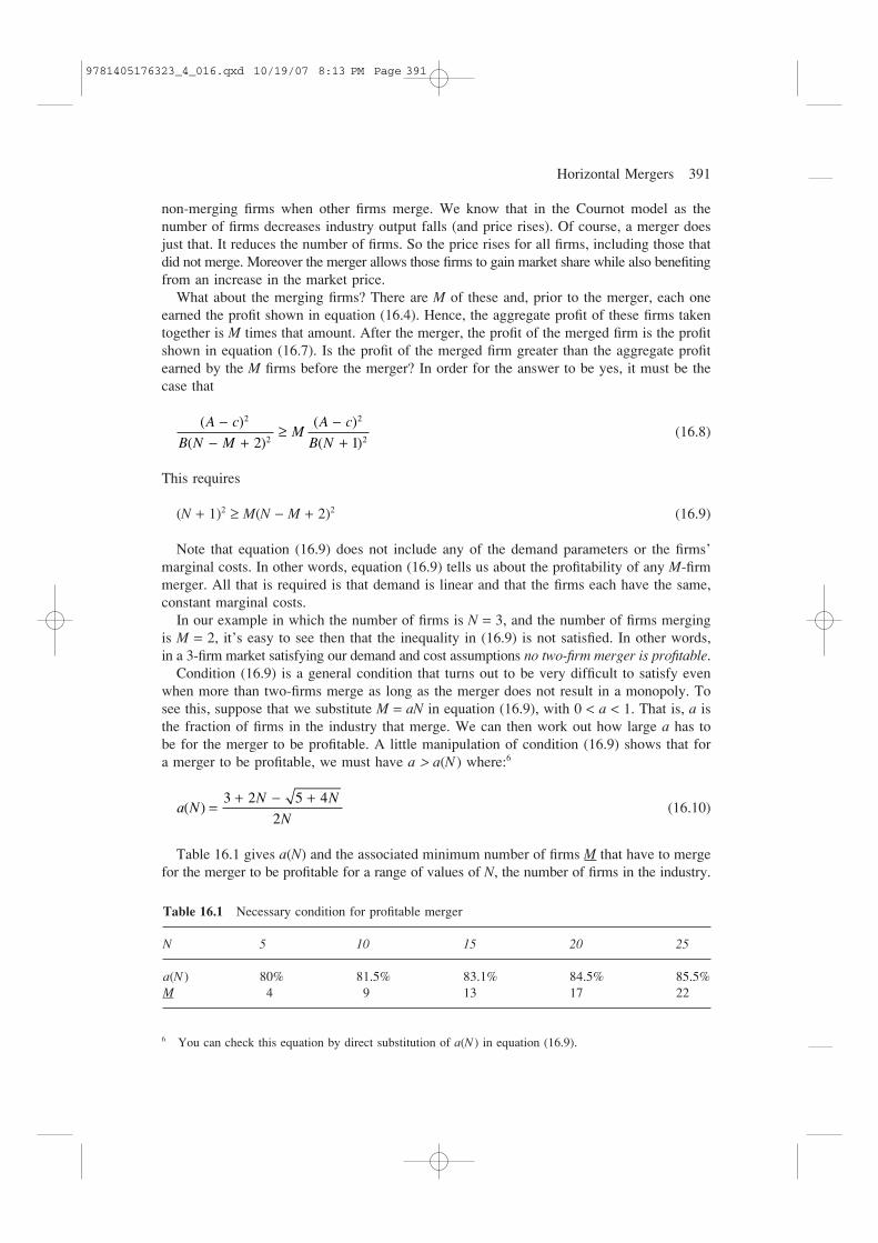
Condition (16.9) is a general condition that turns out to be very difficult to satisfy evenwhen more than two-firms merge as long as the merger does not result in a monopoly. Tosee this, suppose that we substitute M = aN in equation (16.9), with 0 < a < 1. That is, a isthe fraction of firms in the industry that merge. We can then work out how large a has tobe for the merger to be profitable. A little manipulation of condition (16.9) shows that fora merger to be profitable, we must have a > a(N ) where:6

(16.10)

Table 16.1 gives a(N) and the associated minimum number of firms M that have to mergefor the merger to be profitable for a range of values of N, the number of firms in the industry.

a NN N

N( ) =

+ − +3 2 5 4

2

( )

( )

( )

( )

A c

B N MM

A c

B N

−− +

≥−+

2

2

2

22 1

6 You can check this equation by direct substitution of a(N ) in equation (16.9).

Table 16.1 Necessary condition for profitable merger

N 5 10 15 20 25

a(N ) 80% 81.5% 83.1% 84.5% 85.5%M 4 9 13 17 22

9781405176323_4_016.qxd 10/19/07 8:13 PM Page 391

Equation (16.10) and Table 16.1 illustrate what has come to be termed the 80 percent rule.For a merger to be profitable in our simple Cournot world of linear demand and identicalconstant costs, it is necessary that at least 80 percent of the firms in the market merge. Theproblem is that a merger of this magnitude would almost never be allowed by the antitrustauthorities.

Suppose that demand for carpet-cleaning services in Dirtville is described by P = 130 − Q.There are currently 20 identical firms that clean carpets in the area. The unit cost of clean-ing a carpet is constant and equal to $30. Firms in this industry compete in quantities.

a. Show that in a Cournot–Nash equilibrium the profit of each firm is π = 22.67.b. Now suppose that six firms in the industry merge. Show that the profit of each firm in

the post-merger Cournot game is π = 39.06. Show that the profit earned by the mergedfirm is insufficient to compensate all the shareholders/owners who owned the 6 originalfirms and earned profit from them in the pre-merger market game.

c. Show that if fewer than 17 firms merge, the profit of the merged firm is not great enoughto buy out the shareholders/owners of the firms who merge.

The merger paradox is that many, if not most, horizontal mergers are unprofitable whenviewed through the lens of our standard Cournot model. Yet, as the events of the 1990s andmore recent years tell us, horizontal mergers appear to happen all the time. What aspect ofreal-world mergers has the simple Cournot model failed to capture? Alternatively, what aspectof the Cournot model is responsible for this prediction that seems at odds with reality?

The critical aspect of the Cournot model that gives rise to the merger paradox is not difficultto find. When firms merge in the Cournot model, the new combined firm behaves after themerger just like any of the remaining firms that did not merge. Thus, if two firms in a three-firm industry merge, the new firm competes as a duopolist. The nonmerging firm in this casehas, after the merger, equal status to the merged firm even though it now faces the com-bined strength of both of its previous rivals.

One cannot help but suspect that, for a merger of any substantial size, either the newlymerged firm is different in some material sense from its unmerged rivals, or the overall market has changed in a way that alters rivals’ behavior. In the next three sections, we exploresuch possible modifications while staying within the basic Cournot framework. Subsequently,we consider mergers in a market with differentiated products.

16.2 MERGERS AND COST SYNERGIES

In developing the merger paradox we assumed that all firms in the market have identicalcosts and that there are no fixed costs. What happens if we relax these assumptions? It seemsreasonable to suppose that if a merger creates sufficiently large cost savings it should beprofitable. In this section we develop an example to show that this can indeed be the case.7


Pra

ctic

e P

robl

em

16.1

7 This is a special case of a much more sophisticated analysis by Farrell and Shapiro (1990) who show ina general setting that for consumers to benefit from a profitable horizontal merger of Cournot firms themerger has to create substantial cost synergies.

9781405176323_4_016.qxd 10/19/07 8:13 PM Page 392


Suppose that the market contains three Cournot firms. Consumer demand is given by

P = 150 − Q (16.11)

where Q is aggregate output, which pre-merger is q1 + q2 + q3. Two of these firms are low-cost firms with a marginal cost of 30 so that total costs at each are given by

C1(q1) = f + 30q1; C2(q2) = f + 30q2 (16.12)

The third firm is potentially high-cost with total costs given by

C3(q3) = f + 30bq3 (16.13)

where b ≥ 1 is a measure of the cost disadvantage from which firm 3 suffers. In these costfunctions f represents fixed costs associated with overhead expenses such as those for mar-keting or for maintaining corporate headquarters. We now consider the effect of a mergerof firms 2 and 3.

16.2.1 The Merger Reduces Fixed Costs

Consider first the case in which b = 1 so that all firms have the same marginal cost of 30.Suppose, however, that after the merger the merged firm has fixed costs af with 1 ≤ a ≤ 2.What this means is that the merger allows the merged firms to economize on overhead costs, for example by combining the headquarters of the two firms, eliminating unnecessaryoverlap, combining R&D functions and economizing on duplicated marketing efforts. These are, in fact, typical cost savings that most firms state that they expect to result froma merger.

Because the merger leaves marginal costs unaffected, this is similar to our first exampleonly now firms also have fixed costs. Accordingly, we know that in the pre-merger marketeach firm earns a profit of $900 − f. In the post-merger market with just two firms, one earns a profit of $1,600 − f while the merged firm earns $1,600 − af. Hence, for this mergerto be profitable, it must be the case that $1,600 − af > $1,800 − 2f which requires that a < 2 − 200/f. What this says is that a merger is more likely to be profitable when fixedcosts are relatively high and the merger gives the merged firm the ability to make “substantial”savings in these costs. Note, however, that even if the merger is profitable for the mergingfirms, consumers are actually worse off as a result of the higher equilibrium price. That samehigher price also raises the profit of the nonmerged firm. Moreover, it is still the case thatthe merged firm loses market share post-merger.

16.2.2 The Merger Reduces Variable Costs

Now consider the case in which the source of the cost savings is not a reduction in fixedcosts but instead a reduction in variable costs which we capture by assuming that b > 1. Inother words, firm 3 is a high variable cost firm. It follows that after a merger of firms 2 and3, production will be rationalized and the high cost operations will be shut down (or redesignedto have the low cost technology). To make matters as simple as possible we will now assumethat there are no fixed costs ( f = 0).

9781405176323_4_016.qxd 10/19/07 8:13 PM Page 393

Once again we assume a Cournot framework. The outputs and profits of the three firmsprior to the merger are:

(16.14)

The equilibrium pre-merger price is8 . Total output is Q = with

each of the low cost firms, 1 and 2, producing a greater amount than their high cost rival,firm 3.

Now, as before, suppose that firms 2 and 3 merge. Since for any b > 1, it is always moreexpensive to produce a unit of output at firm 3 than it is at firm 2, all production will betransferred to firm 2’s technology. The result is that the market now contains two identicalfirms, 1 and 2, each with marginal costs of $30. Accordingly, in the post-merger industry,each firm produces 40 units, the product price is $70 and each firm earns $1,600.

Is this a profitable merger? For the merger to increase aggregate profit of the merged firmsit must be the case that

(16.15)

You can check that this simplifies to

(16.16)

The first bracketed term in equation (16.16) has to be positive for firm 3 to have been inthe market in the first place (see footnote 8). So the merger is profitable provided that thesecond bracket is also positive, which requires that b > 19/15. In other words, a merger betweena high-cost and a low-cost firm will be profitable provided that the cost disadvantage of thehigh-cost firm prior to the merger is “large enough.” In the case at hand, large enough meansthat firm 3’s unit cost is at least 25 percent greater than firm 2’s unit cost. However, as wehave already demonstrated, whether the merger is profitable or not, the price rises and con-sumers are made worse off.

Together, our analysis of a merger that generates fixed cost savings and one that gener-ates variable cost savings makes clear that mergers can be profitable when the cost savingsare great enough. However, there is no guarantee that consumers gain from such a merger.Admittedly, the merger removes a relatively inefficient firm technology but it also reducescompetitive pressures between the remaining firms. Farrell and Shapiro (1990) demonstratethat in the Cournot setting used here, the cost savings necessary to generate a gain for con-sumers are much larger than those needed simply to make the merger profitable. In turn, thissuggests that we should be skeptical of cost savings as a justification of the benefits to con-sumers of horizontal mergers.

25

27 3 15 19 0( )( )− − >b b

160090 30

16

210 90

16

2 2( ) ( )−

++

−⎛⎝⎜

⎞⎠⎟

b b> 0

390 30

4

− bP

bC =+210 30

4

q qb

qbC C C

1 2 3 1

90 30

4

210 90

4= =

+=

−; and π CC C Cb b

= =+

=−( )

;( )

π π2

2

3

290 30

16

210 90

16


8 Note that this equilibrium only exists only if there is a limit on the disadvantage b for firm 3. Specifically,firm 3’s pre-merger output will be positive only if b < 210/90 = 7/3, otherwise it will not operate in thismarket in the first place.

9781405176323_4_016.qxd 10/19/07 8:13 PM Page 394


Research by both Lichtenberg and Siegel (1992) and Maksimovic and Phillips (2001) findsthat merger related productivity gains and therefore marginal cost savings, while real, aretypically no more than 1 to 2 percent. Salinger (2005) expresses even more doubt that fixedcost savings are substantial. Beyond all this it is also worth noting that even with cost sav-ings, part of our initial paradox still remains since large profit gains continue to accrue tothe firms that do not merge. Why should a firm incur the headaches of merging if it canenjoy many of the same benefits by free-riding on other mergers?9

Return to the market for carpet-cleaning services in Dirtville, now described by the demandfunction P = 180 − Q. Suppose that there are currently 3 firms that clean carpets in the area.The unit cost of cleaning a carpet is constant and equal to $30 for 2 firms and is $30b forthe third firm, where b ≥ 1. In addition, all firms have fixed overhead costs of $900. Firmsin this industry compete in quantities.

a. What is the Cournot–Nash equilibrium price and what are the outputs and profits of eachfirm? What is the upper limit on b for the third firm to be able to survive?

b. Now suppose that a low-cost firm merges with the high-cost firm. In doing so, the fixedcosts of the merged firm become $900a with 1 ≤ a ≤ 2. What is the post-merger equi-librium price? What are the outputs of the non-merged and the merged firms?

c. Derive a relationship between a and b that is necessary to guarantee that the profit earnedby the merged firm is sufficient to compensate all the shareholders/owners who ownedthe two original firms and earned profit from them in the pre-merger market game. Graphthis relationship and comment on it.

16.3 THE MERGED FIRM AS A STACKELBERG LEADER

If cost efficiencies are not a likely way to resolve the merger paradox, then perhaps a resolu-tion can be found in some other change that gives the merged firm an advantage. One pos-sibility is that merged firms become Stackelberg leaders in the post-merger market.10 Recallfrom our discussion in section 11.1 that the source of a Stackelberg leader firm’s advantage isits ability to commit to an output before output decisions are taken by the follower firms. Thispermits a leader to choose an output that takes into account the reactions of the followers.

Let us assume that a merged firm acquires a leadership role and see whether this assump-tion can help resolve the merger paradox. Certainly, such a role seems plausible. After all,the new firm has a combined capacity twice that of any of its non-merged rivals, and somight well be able to act as a Stackelberg leader. Will this be enough to make a mergerprofitable? If so, what will be the response of other firms? Will they also have an incentiveto merge? If they do, will their merging undo the profitability of the first merger and thereby,if firms are foresighted, discourage them from merging in the first place?

9 Perry and Porter (1985) assume that each firm’s cost schedule declines with the total amount of capitalit owns. Hence, by merging and gaining more capital, a firm lowers its costs. The scarcity of capitalmakes it difficult for other firms to do this and, because of rising costs, to free-ride as much on the merger of rivals.

10 This analysis draws on the model A. F. Daughety (1990) who suggested this role for the merged firms.

Pra

ctic

e P

robl

em

16.2

9781405176323_4_016.qxd 10/19/07 8:13 PM Page 395

Suppose that demand is of the usual linear form: P = A − BQ. There are N + 1 firms inthe industry and each of the N + 1 firms has a constant marginal cost of c. Again from sec-tion 9.4 we know that the equilibrium is described by the following equations:

and (16.17)

The profit of each firm, (P − c)qi is therefore:

(16.18)

Suppose now that two of these firms merge and, as a result, become a Stackelberg leader.There will then be F, which is equal to N − 1, follower firms and one leader firm so that we now have N firms in total. Of course, the Stackelberg leader is able to choose its outputfirst in a two-stage game. In stage one, the leader chooses its output Q L. In the second stage, the follower firms independently choose their outputs in response to that chosen bythe leader.

To find the equilibrium, we work through the game backwards. Accordingly, we considerthe second stage of the game in which the follower nonmerged firms make their output deci-sions in response to the output choice QL of the leader or merged firm. We use the notationQF− f to denote the aggregate output of the follower firms other than f, and denote the out-put of follower firm f by qf. Aggregate output of all firms is Q = QL + QF− f + qf. Moreover,the residual demand for firm f, which is the demand left after taking into account the out-puts of the leader and the followers other than firm f is:

P = [A − B(QL + QF− f)] − Bqf (16.19)

Marginal revenue for firm f is, therefore,

MRf = [A − B(QL + QF− f)] − 2Bqf . (16.20)

Equating this with marginal cost gives the best response function for firm f:

(16.21)

Equation (16.21) is the best response of a follower firm to both the output of the leaderand the output of all the other follower firms. Since all follower firms are identical, symmetry demands that in equilibrium the output of each of the follower firms must be identical. The group of followers excluding the firm f has F − 1 = N − 2 firms. Therefore,Q*F− f = (N − 2)qf*. Substituting this into equation (16.21) and simplifying gives the optimaloutput for each non-merged follower firm as a function of the aggregate output of the leadergroup of merged firms:

(16.22)qA c

BN

Q

Nf

L

* =−

−

A Bq BQ BQ c qA c

Bf

LF f f*− − − = ⇒ =

−−2

2−− − −Q QL

F f

2 2

π i

A c

B N

( )

( )=

−+

2

22

PA N c

N

( )=

+ ++

1

2Q

N A c

N B

( )( )

( )=

+ −+1

2q

A c

N Bi ( )

=−

+⇒

2


9781405176323_4_016.qxd 10/19/07 8:13 PM Page 396


The aggregate output of all followers as a function of the output of the leader is then

(16.23)

We can use the same basic technique to determine the output for the leader firm in stageone of the game. The residual inverse demand function for the leader firm is dependent uponthe output of all the other firms, which is given in equation (16.23). So, the demand func-tion facing leader firm l:

P = A − B(Q F + QL )

(16.24)

Its associated marginal revenue function is

MRL (16.25)

Equating this marginal revenue with marginal cost allows us to solve for the leader firm’soptimal output:

(16.26)

You will by now recognize that the output level in equation (16.26) is just the output levelchosen by a uniform-pricing monopolist. This is, of course, a standard result for a singleleader model with linear demand and constant costs. In turn, this implies the following indus-try equilibrium values:

and

(16.27)

Profits for the leader and for each follower firm are then:

and (16.28)

A comparison of equation (16.28) with (16.18) reveals that for any industry initially com-prised of three or more firms and characterized by symmetric Cournot competition, a two-firm merger that creates a Stackelberg leader will be profitable. This seems to resolve themerger paradox. However, equations (16.28) and (16.18) also show that the unmerged firms

π F A c

BN

( )=

− 2

24π L A c

BN

( )=

− 2

4

PA N c

N

( )=

+ −2 1

2

qA c

BNQ

N A c

BNQf

F* ;( )( )

;=−

=− −

=2

1

2

( )( );Q Q

N A c

BNL F+ =

− −2 1

2

MR c QA c

Bl

L= ⇒ =−

2

= −− −

−( )( )

AN A c

N

B

NQL1 2

= −− −

−( )( )

AN A c

N

B

NQL1

= −− −

−−⎡

⎣⎢⎢

⎤

⎦⎥

( )( ) ( )A B

N A c

BN

N Q

N

L1 1

⎥⎥− BQL

Q N qN A c

BN

N QFf( ) *

( )( ) ( )= − =

− −−

−1

1 1 LL

N

9781405176323_4_016.qxd 10/19/07 8:13 PM Page 397

who have become followers are definitely worse off as a result of the merger. We may there-fore expect some response from these firms.

Furthermore, if we compare the market price and output in (16.17) with that in (16.27),we find that while the merger has raised the profit of the merging parties, it also has low-ered price. Hence, the merger is good for consumers. Hence, we may have replaced one para-dox with another. We now have a model in which a merger is profitable, but that model alsoremoves a principal reason why the antitrust authorities should object to such a merger.

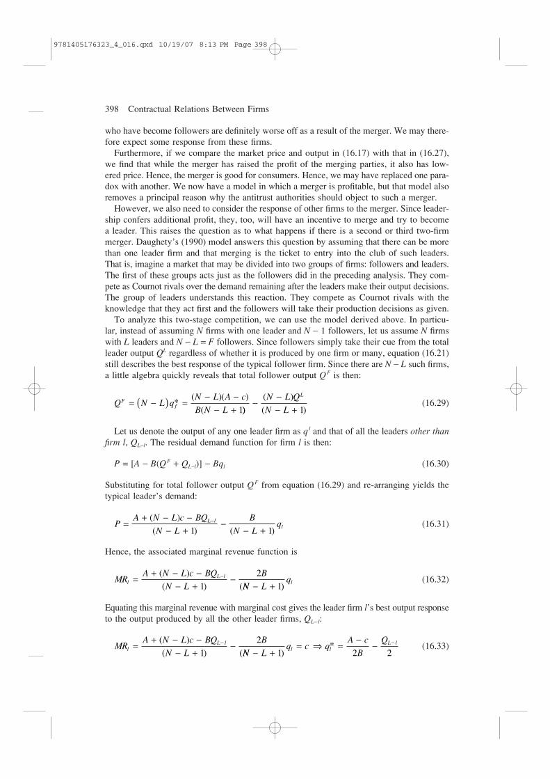
However, we also need to consider the response of other firms to the merger. Since leader-ship confers additional profit, they, too, will have an incentive to merge and try to becomea leader. This raises the question as to what happens if there is a second or third two-firmmerger. Daughety’s (1990) model answers this question by assuming that there can be morethan one leader firm and that merging is the ticket to entry into the club of such leaders.That is, imagine a market that may be divided into two groups of firms: followers and leaders.The first of these groups acts just as the followers did in the preceding analysis. They com-pete as Cournot rivals over the demand remaining after the leaders make their output decisions.The group of leaders understands this reaction. They compete as Cournot rivals with theknowledge that they act first and the followers will take their production decisions as given.

To analyze this two-stage competition, we can use the model derived above. In particu-lar, instead of assuming N firms with one leader and N − 1 followers, let us assume N firmswith L leaders and N − L = F followers. Since followers simply take their cue from the totalleader output QL regardless of whether it is produced by one firm or many, equation (16.21)still describes the best response of the typical follower firm. Since there are N − L such firms,a little algebra quickly reveals that total follower output QF is then:

(16.29)

Let us denote the output of any one leader firm as q l and that of all the leaders other thanfirm l, QL−l. The residual demand function for firm l is then:

P = [A − B(QF + QL−l)] − Bql (16.30)

Substituting for total follower output Q F from equation (16.29) and re-arranging yields thetypical leader’s demand:

(16.31)

Hence, the associated marginal revenue function is

(16.32)

Equating this marginal revenue with marginal cost gives the leader firm l’s best output responseto the output produced by all the other leader firms, QL− l:

(16.33)MRA N L c BQ

N L

Bl

L l( )

( ) (=

+ − −− +

−−

1

2

NN Lq c q

A c

B

Ql l

L l

)*

− += ⇒ =

−− −

1 2 2

MRA N L c BQ

N L

Bl

L l( )

( ) (=

+ − −− +

−−

1

2

NN Lql)− + 1

PA N L c BQ

N L

B

NL l( )

( ) (=

+ − −− +

−−

−

1 )Lql+ 1

Q N L qN L A c

B N LF

f*( )( )

(= −( ) =

− −− + 1))

( )

( )−

−− +

N L Q

N L

L

1


9781405176323_4_016.qxd 10/19/07 8:13 PM Page 398


Once again, we can take advantage of the fact that since all of the leader firms have thesame costs they will each produce the same level of output in equilibrium. Because thereare L − 1 leaders other than firm l, this gives the symmetry condition Q*L− l = (L − 1)ql* whichwhen substituted into equation (16.33) allows us to solve for the output chosen in stage oneby each merged firm in the leader group:

and (16.34)

Substituting the value for QL into equation (16.29) we can then find total follower outputQF and individual output for each follower q f* = QF/(N − L). These are:

and (16.35)

Finally, summing QL and QF together yields total market output Q and, via the demand curve,the equilibrium price P:

and (16.36)

In turn, the price and output equations imply that in an industry comprised of N firms intotal L of which are leaders, the price-cost margin (P − c) and the profits for the typicalleader firm (P − c)q l* and typical follower firm (P − c)q f* are:

; ; and

(16.37)

You can readily confirm that the profit values shown in equation (16.37) for the general caseof N total firms with L leaders, yields the same profits as those given in equation (16.28) forthe special case of N firms and L = 1 leader.

It is clear from the profit equations in (16.37) that the leader firms are more profitablethan the nonmerged followers. Yet that is not the real issue facing two firms that are con-templating merger. The question is whether one more merger is profitable, given that therewill then be one more leader, two fewer followers, and one less firm in total. This is whywe have written the profit expressions as functions of N and L. The point is that an addi-tional merger creates two countervailing forces. On the one hand there are fewer firms intotal, which ought to increase profits, but there are also more leaders, which ought to decreasethe profits of the leaders. Which force is greater?

Suppose there is an additional merger of two followers, so that the newly merged firmand all other leaders earn profit given by equation (16.37) with N replaced by N − 1 and L replaced by L + 1 to give π L

l (N − 1, L + 1). For there to be an incentive to merge, thisprofit must exceed the combined profit earned by the two follower firms prior to the merger.

π F N LA c

B L N L( , )

( )

( ) ( )=

−+ − +

2

2 21 1

π L N LA c

B L N L( , )

( )

( ) ( )=

−+ − +

2

21 1P c

A c

L N L( )( )− =

−+ − +1 1

PA N NL L c

L N L

( )

( )( )=

+ + −+ − +

2

1 1Q Q Q

N NL L A c

B LT L F ( )( )

( )= + =

+ − −+

2

1 (( )N L− + 1

QN L A c

B L N LF ( )( )

( )( )=

− −+ − +1 1

qA c

B L N Lf* ( )( )

=−

+ − +1 1

Q LqL A c

B LL

l*( )

( )= =

−+ 1

qA c

B

Lq q

A c

Bl l l*

( )* *

(=

−−

−⇒ =

−2

1

2 LL )+ 1

9781405176323_4_016.qxd 10/19/07 8:13 PM Page 399

This latter profit is 2πfF(N, L). So, the merger will be profitable if the following condition

is satisfied:

(16.38)

This simplifies to the condition

(L + 1)2(N − L + 1)2 − 2(L + 2)2(N − L − 1) > 0 (16.39)

Note that this condition does not include the demand parameters A and B or the marginalcost c. In other words, the profitability or otherwise of this type of merger depends only onthe number of leaders and followers, not on the precise demand and cost conditions.

As turns out, the condition in (16.39) is always met. This is shown in Table 16.2 wherewe have calculated the left-hand side of equation (16.39) for any two-firm merger for a rangeof values of N and L. In other words, starting from any configuration of leaders and fol-lowers, an additional two follower firms always wish to merge.

This result is encouraging. It says that our model offers one way to resolve the merger paradox. A merger raises the profit of the two merging firms by allowing them to take a position as one of, perhaps several, industry leaders. Moreover, the fact that such a merger is always profitable also helps us to understand better the domino effect so often observed within an industry. Once one firm merges and becomes a leader, the remaining firms will wish to do the same rather than watch their output and their profits besqueezed.

π L N LA c

B L N L( , )

( )

( ) (− + =

−+ −

1 12

2

2 −−> =

−+ −)

( , )( )

( ) (12

2

1

2

2π F N L

A c

B L N LL )+ 1 2


Table 16.2 Profit effect of two follower firms merging to become a leader, given N followers andL eaders prior to the merger

Original Original number of firms Nnumber ofleaders L 5 10 15 20 25 30 35 40 45 50

2 80 505 1,380 2,705 4,480 6,705 9,380 12,505 16,080 20,1054 865 2,880 6,145 10,660 16,425 23,440 31,705 41,220 51,9856 841 3,876 9,361 17,296 27,681 40,516 55,801 73,536 93,7218 529 3,984 11,489 23,044 38,649 58,304 82,009 109,764 141,569

10 3,204 12,049 26,944 47,889 74,884 107,929 147,024 192,16912 1,920 10,945 28,420 54,345 88,720 131,545 182,820 242,54514 8,465 27,280 57,345 98,660 151,225 215,040 290,10516 5,281 23,716 56,601 103,936 165,721 241,956 332,64118 2,449 18,304 52,209 104,164 174,169 262,224 368,32920 12,004 44,649 99,344 176,089 274,884 395,72922 6,160 34,785 89,860 171,385 279,360 413,78524 23,865 76,480 160,345 275,460 421,825

9781405176323_4_016.qxd 10/19/07 8:13 PM Page 400


Return again to the town of Dirtville where the inverse demand for carpet-cleaning servicesis described by P = 130 − Q. Once again assume that there are 20 identical firms that cleancarpets in the area, and the unit cost of cleaning a carpet is constant and equal to $30. Firmsin this industry compete in quantities.

a. Show that in a Cournot equilibrium the aggregate number of carpets cleaned is Q = 95.24.What is the equilibrium price?

b. Suppose that five two-firm mergers occur, that these five merged firms become leaderfirms, and the remaining ten nonmerged firms are followers. Now there are 15 firms in the industry. Work through the model just described and show that in the two-stagegame a leader firm cleans 16.67 carpets and each follower firm cleans 1.51 carpets.Leadership certainly has its benefits! Show that the total industry output in this case willbe Q = 98.45. What is the equilibrium price now?

c. If after the five two-firm mergers took place there were no leadership advantage con-ferred to the merged firms, then we would have 15 firms competing like Cournot firmsin the market. Show that in this case aggregate output is Q = 93.75.

While the Daugherty model can resolve the merger paradox it does leave unanswered thequestion as to whether such mergers are in the public interest. Is there some point at whichfurther mergers are harmful to consumers? The answer to this question can be most easilyderived from the price-cost relation P − c shown in equation (16.36). Since marginal cost cis constant, any rise or fall in P will be reflected in a rise or fall of P − c.

With L leader merged firms and N − L follower non-merged firms the price-cost differ-

ential is . An additional two-firm merger increases L to L + 1 and

decreases N to N − 1, so that the price-cost margin is now . So for this

additional merger to benefit consumers it must be the case that:

(16.40)

What this tells us is that an additional two-firm merger benefits consumers only if N > 3(L + 1) or, equivalently, L < N/3 − 1. In other words, a two-firm merger that increasesthe number of leaders benefits consumers only if the current group of leaders contains fewerthan a third of the total number of firms in the industry. We know from Table 16.2 that a two-firm merger that creates a leader will always be profitable. Yet, as also just shown,such a merger will be harmful to consumers once the leader group includes one-third or more of the industry’s firms. In other words, some mergers are bad—at least for consumers.Accordingly, we now have a model that both resolves the merger paradox and explains whythe antitrust authorities are correct to worry about anticompetitive mergers.

For example, return to Practice Problem 16.3 in which we had five leader firms and tenfollower firms cleaning carpets in Dirtville. In that scenario we know that the equilibrium

⇒ + − + < + − − ⇒( )( ) ( )( )L N L L N L1 1 2 1 ( )N L− + >3 1 0

A c

L N L

A c

L N( )( ) ( )(

−+ − −

<−

+ −2 1 1 LL )+ 1

A c

L N L( )( )

−+ − −2 1

A c

L N L( )( )

−+ − +1 1

Pra

ctic

e P

robl

em

16.3

9781405176323_4_016.qxd 10/19/07 8:13 PM Page 401

price for cleaning a carpet is $31.55. Now suppose that two additional firms merge to jointhe leadership group. We then have a market structure of six leaders and eight followers. Inthis case, the equilibrium price for cleaning a carpet is $31.60. This merger harms the con-sumers in Dirtville.

Daughety’s (1990) model solves the merger paradox and gives rise to a merger wave byassuming an asymmetry between newly merged firms and their remaining unmerged rivals.The former gain membership in the club of industry leaders. However, this is a rather strongassumption. While some mergers may create corporate giants with an ability to commit to large production levels, it is far from obvious that every two-firm merger should have thisleadership role regardless of which two firms are joined and irrespective of the number of


Reality Checkpoint

It’s a Gusher! Merger Mania in the Oil Industry

In August of 1998, British Petroleum or BP announced plans to merge with Amocoanother large oil firm although not quite as largeas BP. The price tag was $48.2 billion makingit, at the time, the biggest industrial merger ever. The new BP-Amoco would control moreoil and gas production within North Americathan any other firm. It would also be the third-largest publicly traded oil firm in the world. (Thelargest firm of all, Saudi Aramco, is not pub-licly traded.)

Reaction from the rest of the oil industrycame swiftly. Within a year, Exxon and Mobilmerged in a deal worth $73.7 billion to becomethe largest publicly traded firm on earth. Thatwas quickly followed by the merger of PhillipsPetroleum and Conoco. Almost simultaneously,Paris-based Total acquired both PetroFina andElf to create TotalFinaElf. Soon after, Chevronacquired Texaco for $36 billion. BP then wenta step further and acquired Arco for $27 bil-lion. The oil merger wave subsided with the economic decline of 2000–1 but even then, didnot die altogether. Chevron acquired Unocal in 2005.

This wave of merger activity concentrated oiland gas refining and marketing into the handsof a noticeably smaller number of firms rela-tive to the situation prior to BP’s purchase ofAmoco. The BP-Amoco merger was then thecatalyst for a major wave of mergers and con-solidations. In turn, this suggests that a com-mon motive must be behind all these mergers.

Yet whether this common factor was thenaked pursuit of market power or simply theprofit-maximizing response of firms to similarproblems is difficult to say. The mergers weretaken at a time when energy prices were quitelow. Oil, for example, was selling at less than$12 per barrel in 1998. Indeed, this low price—and the low energy company profits thatwent with it—is probably the reason that noneof the mergers was seriously challenged byantitrust authorities. However, oil prices andprofits have risen dramatically since that time.This could reflect the demand growth drivenby a rising world economy coupled withimproved cost efficiency that the mergers generated. However, it could also reflect theexploitation of newly enhanced market power.In this connection, a recent study by theGovernment Accounting Office (GAO) foundthat increased concentration could account for only a few cents of the large rise in whole-sale gasoline prices. The rest appeared to bedemand and cost pressures. If this view is cor-rect, lower oil and gas prices are only likely ifconservation measures reduce energy demand.

Sources: Jim Wells, “Energy Markets: FactorsContributing to Higher Gasoline Prices,” Statementof Director of Natural Resources and Environ-ment, General Accounting Office, to U. S. SenateJudiciary Committee, February 1, 2006; and B.Bahree, C. Cooper, and S. Liesman, “BP to BuyAmoco in Biggest Industrial Merger Ever,” Wall StreetJournal, August 12, 1998, p. A1.

9781405176323_4_016.qxd 10/19/07 8:13 PM Page 402


leaders already present. In principle, Daughety’s (1990) model implies that in an industryof ten firms there could be, say, eight leaders. It seems odd though to imagine a configura-tion with so many leaders and so few followers. Moreover, it leaves unanswered the ques-tion as to what happens if two leaders merge. Does this merger create a super-leader?

It is also worth noting that while production is sequential in Daughety’s (1990) model,merging is not. While leader firms choose production first, it is not accurate to describe thedecision to merge in a sequential way. The model simply says that for any market configura-tion, if a two-firm merger creates an industry leader, all follower firm pairs will wish to mergeas well. One pair does not merge only after it sees another pair merge. Instead, at any sin-gle point in time, merging is a dominant strategy and, absent any antitrust intervention, allfollower firms will pursue it. Again, this is not because of any new cost savings or productdevelopment. It is simply because merging confers leadership status. Thus, Daughety’s (1990)model does not give rise to the sporadic merger waves that we often see as much as it sug-gests an ever-present tendency for the industry to become more concentrated.

To capture the idea that merger decisions may be explicitly sequential, i.e., that the deci-sion of one firm pair to merge is a catalyst for another pair to do the same, a number ofpapers including Nilssen and Sørgaard (1998), Fauli-Oller (2000) and Salvo (2006) have recentlypresented models in which a sudden change in cost or product qualities give rise to mergeropportunities that are only profitable if other mergers also occur. It is difficult for this tohappen in a simultaneous game because each potential merger pair cannot be sure if otherswill also merge. However, in a sequential game, some firms get to make their merger deci-sion knowing for certain that others have already merged. This greatly enhances the likeli-hood of a successful merger.

We illustrate the sequential merger model with a simplification of the Fauli-Oller (2000)model. Consider a four-firm industry characterized by Cournot competition. Initially, all ofthese firms are high-cost firms with constant unit cost ch = c. Suppose that two firms havehad a technical breakthrough that allows them to become low-cost firms with low constantunit cost c l = 0. Industry demand is described by: P = A − Q.

Using the Cournot model in section 9.4, it is easy to show that the initial, post-innovationequilibrium is described as follows:

(16.41)

As a result, each firm earns a profit π of

and (16.42)

Now consider two possible mergers. In each merger, a low-cost firm buys a high-cost firmand the two then operate as a single low-cost producer. The merger permits the transfer ofproduction from the high-cost plant to the low-cost one. If both of these mergers happen,there will be just two low-cost firms and the industry equilibrium will have the followingfeatures:

and (16.43)π jl A

j; ,=⎛⎝⎜

⎞⎠⎟

=3

1 22

qA

j QA

PA

jl ; , ; ;= = ⇒ = =

31 2

2

3 3

π jl A c

j; ,=+⎛

⎝⎜⎞⎠⎟

=2

51 2

2

π ih A c

i; ,=−⎛

⎝⎜⎞⎠⎟

=3

51 2

2

qA c

i qA c

jih

jl; , ;=

−= =

+3

51 2

2

5== ⇒ =

−=

+, ;1 2

4 2

5

2

5Q

A cP

A c

9781405176323_4_016.qxd 10/19/07 8:13 PM Page 403

Observe that we must have A > 3c for the pre-merger equilibrium to involve any positiveoutput for the high-cost firms. In turn, this means that the expression for π l

j in (16.43) willalways exceed the sum of π h

i and π lj from (16.42). That is, a merger between one pair of

high- and low-cost firms will be profitable so long as the other pair also merges.For example, suppose that A = 100 and c = 10. Then in the pre-merger equilibrium, high-

cost firms each earn $196 in profit and low-cost firms each earn $576 in profit. So, the pre-merger profit of any low-cost and high-cost pair is $772. If both such pairs merge, however,the profit of the merged firm rises to $1,111.11. Clearly, this is the preferable outcome fromthe viewpoint of the two firms.

A potential problem is that one merger will be unprofitable just as the merger paradoxsuggests. If only one low-cost and high-cost pair merges, the new equilibrium will be:

(16.44)

The profit of the remaining high-cost firm and of each of the two low-cost firms, respect-ively, will be:

and (16.45)

Thus, in our numerical example, the remaining high-cost firm will benefit from the priceincrease the merger causes and see its profit rise to $306.25. The same is true for the unmergedlow-cost firm whose profit will rise to $756.25. The merged firm will also now earn $756.25as it transfers production from the acquired high-cost plants to the more efficient low-costones. However, this is less than the $772 earned as two separate companies in the pre-mergerequilibrium. Therefore, no one pair has an incentive to merge on its own. As a result, itseems difficult to reach the two-merger equilibrium outcome even though this would raiseprofits for all involved.

Let us now introduce a sequential structure to the game, where firms do not make themerger decision simultaneously but, instead, sequentially. Thus, the second merger pair getsto make its decision after the first pair. Moreover, the first pair knows this. The rules of thegame—in this case, simultaneous versus sequential play—matter a lot for the outcome.

Consider again the outcome when only one firm-pair merges from equation (16.45). Inour numerical example, this results in the remaining high-cost firm earning $306.25 in profitwhile the merged firm and its low-cost rival each earn $756.25. Knowing that one mergerhas already taken place, the second merger pair now has a choice of either staying in thisequilibrium or merging themselves in which case the market outcome would have two, low-cost firms as described by equation (16.43). If they merge, this second merged new firm willearn a profit of $1,111.11, which is an increase over the $1,062.50 in combined profit thatthe two firms will earn if they do not merge. Conditional on the first merger taking placethen, the second merger is profitable. In effect, the sequential nature of the game allows thefirst pair to commit credibly to merging. In turn, that means that the second merger pair doesnot have to worry that in merging they may be acting alone.

The first pair of merging firms can work through the foregoing logic as well as we can.These firms will therefore understand that their merger will also not be the only one but,instead, be followed by another in which case they too will see their combined profits rise

π jl A c

j; ,=+⎛

⎝⎜⎞⎠⎟

=4

1 22

π ih A c

i; ,=−⎛

⎝⎜⎞⎠⎟

=3

41 2

2

qA c

qA c

jhjl

1

3

4 41 2; ; ,=

−=

+= ⇒ ;Q

A cP

A c=

−=

+3

4 4


9781405176323_4_016.qxd 10/19/07 8:13 PM Page 404


to $1,111.11. As a result, we can expect a merger wave in which first one pair merges andthen the second pair merges. Suppose that in this wave, mergers are motivated by a low-cost firm buying a high-cost firm. Since the profit foregone by a high-cost firm is $306.25and that foregone by a low-cost firm is $756.25 when each is part of the second merger, andsince the order of mergers is arbitrary, there will be a sequence of mergers in which theacquisition price is somewhere between $306.25 and $354.86 (= $1,111.11 − $756.25), andthe industry will end up with just two, low-cost firms. The merger wave is not, however,desirable for consumers. The industry price rises from $24 to $33.33.

The foregoing story is not limited to just two mergers or to models of Cournot competi-tion. Once cost asymmetries or product quality differences are introduced, we can constructsequential merger models that lead to merger waves for a large number of firms in a vari-ety of settings, e.g., Nilssen and Sørgaard (1998) and Salvo (2006), and these mergers arealso anticompetitive. This approach offers another resolution to the merger paradox not simply because it demonstrates why mergers may happen but, in addition, why they oftenhappen in sequential waves. As with Daughety’s (1990) model, these models also justifyconcern over the impact that mergers may have on consumer prices.

16.4 HORIZONTAL MERGERS AND PRODUCTDIFFERENTIATION

Our analysis of mergers has so far been set in the Cournot framework of identical productsand quantity competition. However, many firms expend considerable effort differentiating theirproducts and this differentiation gives them some latitude in setting their price. Accordingly,we also need to consider the incentives for and the impact of mergers in industries in whichfirms produce and market differentiated products.

It is particularly important to explore the merger phenomenon in differentiated productmarkets because often firms are price setters in such markets and the nature of competitionis different with price competition than with quantity competition. In quantity competitionfirms’ best response functions are downward sloping, i.e., quantities are strategic substitutes.Thus, when merging occurs, the non-merged firms want to increase their outputs in responseto the lower output produced by the merger. This response undermines the effectiveness ofthe merger. By contrast, with price competition best response functions are upward sloping:prices are strategic complements. A merger leading to an increase in the merged firms’ price(s)will encourage the non-merged firms also to increase their prices, potentially strengtheningthe effectiveness of the merger.

We develop this intuition more explicitly using two different approaches to product dif-ferentiation. The first approach is to extend our standard linear demand representation ofconsumer preferences to incorporate product differentiation. The second is to adopt the spatial model of horizontal differentiation, which we first introduced in Chapter 4 and thenrevisited in Chapter 10.11

11 The spatial model was first formulated in Hotelling (1929), and subsequently extended in Schmalensee(1978) and Salop (1979). We saw in Chapters 4, 7, and 10 that this sort of spatial model has proveninsightful in analyzing a variety of topics in industrial organization, including brand proliferation in theready-to-eat breakfast cereal industry, Schmalensee (1978), and the effects of deregulation of transportservices such as airlines or passenger buses, Greenhut et al. (1991). It is not surprising that the spatialmodel is also useful in analyzing mergers of firms selling differentiated products.

9781405176323_4_016.qxd 10/19/07 8:13 PM Page 405

16.4.1 Bertrand Competition and Merger with Linear Demand Systems

Suppose that there are three firms in the market, each producing a single differentiated prod-uct.12 Inverse demand for each of the three products is assumed to be given by:

p1 = A − Bq1 − s(q2 + q3)

p2 = A − Bq2 − s(q1 + q3) (s ∈ [0, B)) (16.46)

p3 = A − Bq3 − s(q1 + q2)

In these inverse demand functions the parameter s, where 0 ≤ s ≤ B, measures how sim-ilar the three products are to each other. If s = 0 the products are totally differentiated. Inthis case, each firm is effectively a monopolist. By contrast, as s approaches B the three prod-ucts become increasingly identical, moving us closer to the homogeneous product case. Wewill also assume that the three firms have identical marginal costs of c per unit. Finally,assume that the three firms are Bertrand competitors, i.e., they compete in prices and settheir prices simultaneously.

We show in Appendix A to this chapter that when these firms compete they each set a

price of and each sell quantity . Profit of

each firm is then

(16.47)

Now suppose that firms 1 and 2 merge but that the merged and non-merged firms continue to set their prices simultaneously. The two previously independent, single-productfirms are now product divisions of a two-product merged firm, coordinating their prices tomaximize the joint profit of the two divisions. The result is that the merged firm sets its

product prices to while the remaining

non-merged firm 3 sets its product price as .

It is straightforward to confirm that the merger increase the prices of all three products,as we might have expected since the merger reduces competitive pressures in the market.However, there remains the question of the merger’s profitability. The profits of each prod-uct division of the merged firm, and of the independent non-merged firm are:

(16.48)

In comparing equations (16.47) and (16.48) we can simplify matters by normalizing A − c = 1 and B = 1, so that profits are functions solely of the degree of product differenti-ation s. It is then easy to confirm that this two-firm merger is profitable for the merged firm

π π1 2

2 22 3

4m m A c B B s B s

B

( ) ( )( )

(= =

− − ++ )( )

;( ) (

2 2 22 2 2 3

2

s B Bs s

A c Bm

+ −=

− −π

ss B s

B s B Bs s

)( )

( )( )

++ + −

3

2 2 22 2 2

pA B s B s cB B s

Bnm3 2

2

2 2

( )( ) ( )

(=

+ − + ++ BBs s )− 2

p pA B s B s c B s Bm m

1 2

2 3 2( )( ) ( )(= =

+ − + + )

( )

++ −

s

B Bs s2 2 22 2

πnm

A c B s B s

B B s*

( ) ( )( )

( )=

− − ++

2

24 2

qA c B s

B B snm*

( )( )

( )=

− ++2 2

pA B s c B s

Bnm*

( ) ( )=

− + +2


12 An excellent example of the full analysis can be found in Davidson and Deneckere (1986).

9781405176323_4_016.qxd 10/19/07 8:13 PM Page 406


and for the non-merged firm. More generally, Davidson and Deneckere (1986) show that ina market containing N firms any merger of M ≥ 2 firms is profitable for the merged firmsand for the non-merged firms. This simple framework of price setting in a product differ-entiated market avoids the merger paradox, suggesting that mergers are both profitable andof potential concern to antitrust authorities unless accompanied by cost efficiencies.

16.4.2 Mergers in a Spatial Market

In the spatial model, a merger between two firms may well bring increased profit for rea-sons similar to those in the previous section. Although merging means that the firms losetheir separate identity, they do not lose the ownership or control of the product varieties theycan offer. For example, the merger of two major banks, Bank of America and Fleet Bank,results in a single new corporate entity. Yet it does not require that the new firm give upany of the locations at which either Bank of America or Fleet currently operate—or that itlose control over the choice of moving some of those locations. Similarly, the acquisitionsome years ago of American Motors by Chrysler did not mean that the Jeep product linedisappeared.

When we consider a firm’s product lines, there is a second source of potential profit increase.The merged firms can now coordinate not just the prices but also the design of their prod-uct line, or in the context of the spatial model, their location choices. Chrysler can redesignthe Jeep line to fit better in its overall range of models. Similarly, Bank of America andFleet can change the locations of their branches in those areas where each formerly oper-ated an outlet quite close to the other.

To investigate the impact of a merger in the spatial model we begin by recalling the basicsetup of the model.13 There is a group of consumers who are uniformly distributed over alinear market of length L. Again, we can think of this as Main Street in Littlesville.However, one small problem with the Main Street analogy is that outlets at either end of themarket can only reach consumers on one side. This restriction introduces an asymmetry inthe model, which we would like to avoid. To make the product differentiated market sym-metric we can bend the ends of the line around until they touch each other, and replace ourstraight line of length L with a circle of circumference L. If we use the spatial model to rep-resent departure times in the differentiated airline market, the circle represents the 24 hoursof the day about which consumers differ in terms of their most preferred time of departure.In all other respects, the spatial model remains as before.

Each consumer has an “address” indicating her location on the circle and, hence, her mostpreferred product type. Each consumer is also willing to buy at most one unit of a particu-lar good. The consumer’s reservation price for her most preferred good is denoted by V.Different varieties of the good are offered by the firms that are also located on Main Street—or, more appropriately, Main Circle.14 A consumer buys from the firm that offers the prod-uct to her at the lowest price, taking into account the costs of transporting the good fromthe firm’s address to the consumer’s. We assume that these transport costs are linear in dis-tance. If the distance between a firm and a consumer is d, the transport costs from the firmto the consumer is td, i.e., t is the transport cost per unit distance. Recall that in the non-geographic interpretation of the model, transport costs become the consumer’s valuation of

13 A more general, but much more complicated version of this analysis can be found in Brito (2003).14 It bears repeating that the spatial or geographic interpretation of this model is only the most obvious one.

See the discussion in Chapter 10.

9781405176323_4_016.qxd 10/19/07 8:13 PM Page 407

the loss of utility incurred by consuming a product with characteristics that are not the con-sumer’s most preferred characteristics.

Suppose that there are five firms selling to a group of N consumers who are distributedevenly around the circle of circumference L. A firm is differentiated only by its location onthe circle, and we assume that the distance between any two neighboring firms is the sameand equal to L/5. Each firm has identical costs given by C(q) = F + cq, where F is fixedcost and c is (constant) marginal cost. In contrast to our earlier merger analysis, we do notset F, the fixed cost, equal to zero, but instead set unit cost c = 0. This simplifies the ana-lysis without losing any generality. What it does do is make it easy to talk about the price-cost margin, which is now just price, denoted by m for mill price.15

No price discrimination

We start by considering the case in which firms do not engage in price discrimination. Thismeans that each firm sets a single mill price m that consumers pay at the firm’s store or milllocation. The consumer then pays the fee for transporting the product back to her location.The full price paid by a consumer who buys from firm i is mi + tdi, where mi is firm i’s millprice and tdi is the consumer’s transport cost (or the utility lost by this consumer in buyinga product that is not “ideal”). Since marginal cost is zero, the net revenue or profit marginearned by firm i on every such sale is mi. Consumers buy from the firm offering the product at the lowest full price. As a result, for any set of mill prices across our five hypo-thetical firms (m1, m2, m3, m4, m5) the market is divided between the firms as illustrated in Figure 16.1. The dotted lines indicate the market division between the firms. Firm 1, forexample, supplies all consumers in the region (r15, r12).

When the firms set their prices noncooperatively and the maximum willingness to pay Vis relatively large, the market is completely covered. That is, every consumer buys from somefirm. Hence, the marginal consumer for any firm is the one who is just indifferent between


15 If the reader is interested in working out the outcome for the case of c ≠ 0, then we note here that ineach case that we examine, the equilibrium price m* that we derive should be replaced by c + m*.

Firm 1

r12

Firm 5

Firm 4

Firm 3

Firm 2

r15

r45

r34

r23

Figure 16.1 Product differentiation: no price discrimination

9781405176323_4_016.qxd 10/19/07 8:13 PM Page 408


buying from that firm and buying from one of the firm’s neighbors.16 We show in Appen-dix B to this chapter that in equilibrium the mill price set by each firm is mi* = tL/5. At thisprice, the profit earned by each firm is

(16.49)

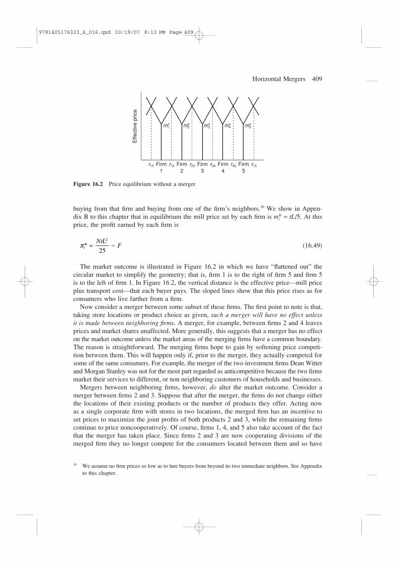
The market outcome is illustrated in Figure 16.2 in which we have “flattened out” the circular market to simplify the geometry; that is, firm 1 is to the right of firm 5 and firm 5is to the left of firm 1. In Figure 16.2, the vertical distance is the effective price—mill priceplus transport cost—that each buyer pays. The sloped lines show that this price rises as forconsumers who live farther from a firm.

Now consider a merger between some subset of these firms. The first point to note is that,taking store locations or product choice as given, such a merger will have no effect unlessit is made between neighboring firms. A merger, for example, between firms 2 and 4 leavesprices and market shares unaffected. More generally, this suggests that a merger has no effecton the market outcome unless the market areas of the merging firms have a common boundary.The reason is straightforward. The merging firms hope to gain by softening price competi-tion between them. This will happen only if, prior to the merger, they actually competed forsome of the same consumers. For example, the merger of the two investment firms Dean Witterand Morgan Stanley was not for the most part regarded as anticompetitive because the two firmsmarket their services to different, or non neighboring customers of households and businesses.

Mergers between neighboring firms, however, do alter the market outcome. Consider amerger between firms 2 and 3. Suppose that after the merger, the firms do not change eitherthe locations of their existing products or the number of products they offer. Acting now as a single corporate firm with stores in two locations, the merged firm has an incentive toset prices to maximize the joint profits of both products 2 and 3, while the remaining firmscontinue to price noncooperatively. Of course, firms 1, 4, and 5 also take account of the factthat the merger has taken place. Since firms 2 and 3 are now cooperating divisions of themerged firm they no longer compete for the consumers located between them and so have

π i

NtLF* = −

2

25

16 We assume no firm prices so low as to lure buyers from beyond its two immediate neighbors. See Appendixto this chapter.

Effe

ctiv

e pr

ice

Firm1

r15 Firm2

r12 Firm3

r23 Firm4

r34 Firm5

r45 r15

m*1 m*2 m*3 m*4 m*5

Figure 16.2 Price equilibrium without a merger

9781405176323_4_016.qxd 10/19/07 8:13 PM Page 409

an incentive to raise the prices of products 2 and 3.17 This will likely lead to the loss of some consumers, namely, those just on the boundaries identified by the points r12 and r34.But provided that the merged firm does not raise prices too much the loss of market sharewill be more than offset by the increased profit margins on their “captive” consumers—theconsumers between the two merging firms. Moreover, the increased prices set by the mergedfirm will induce a similar increase in prices set by firms 1, 4, and 5. Such a response reducesthe loss of market share that the merged firm actually suffers making the price increase allthe more profitable.

Again we show in Appendix B that the merger leads to a new equilibrium with the following prices:

(16.50)

Profits to each product are

(16.51)

This equilibrium is illustrated in Figure 16.3. Comparison with equation (16.37) confirmsthat this merger is profitable for the merging firms.

The equilibrium we have identified is based upon the assumption that the merged firmsleave their product lines unchanged after the merger. What do we expect to happen if werelax this assumption? It turns out that the answer to this question depends upon the precisenature of transport costs. Consider the product location choice facing the newly merged firm2 and firm 3. The firm faces a trade-off. On the one hand, relocating products 2 and 3 nearerto products 1 and 4, respectively gives the merged firm two advantages. First, it softens thecompetition between the merged firm’s own two product lines, so that when the firm triesto reach out to customers near the boundary with a lower price there is less of a fear of sim-ply “robbing Peter to pay Paul.” Second, the move also makes it easier for the firm to stealsome customers away from its true rivals, firms 1 and 4.18 On the other hand, relocating

π π π π2 3

2

1 4

361

7 200

4* *

,; * *= = − = =

NtLF

99

900

169

3 600

2

5

2NtLF

NtLF; *

,− = −π

m mtL

m mtL

m2 3 1 4 5

19

60

14

60* * ; * * ; *= = = = =

13

60

tL


17 If the merger leaves products 2 and 3 under the control of separate, competing product divisions, priceswill not change. It is important, in other words, that the merged firms take advantage of the opportunitythey now have to coordinate their prices.

18 There is one complication that we have ignored in this discussion. Judd (1985) argues that a merger thatcreates a multiproduct firm, as for example a merger of firms 2 and 3, may not be sustainable. The intu-ition is as follows: Assume that an entrant comes in exactly at firm 3’s location after the merger of firms2 and 3. Price competition will drive the price for this product down to marginal cost, in which case theentrant and the incumbent earn zero profits at this location (ignoring fixed costs). But the merged firmalso loses money at the neighboring location 2 since the price war with the new entrant forces it to reducethe price there as well. If the merged firm were to close down its location 3 product, the entrant willraise price above marginal cost, and so the merged firm can raise the price at location 2. There is, inother words, a stronger incentive for the merged firm to exit location 3 than for the entrant to do so.Hence, this kind of multiproduct merger may not be sustainable because it is not credible. This argu-ment turns, however, on two important assumptions: that entry costs are not recovered on exit and thatthe merged firm has no incentive to try to develop a reputation for toughness. If only part of the entrycosts are sunk (unrecoverable costs), or if reputation is important, the merged firm can sustain the multi-product configuration.

9781405176323_4_016.qxd 10/19/07 8:13 PM Page 410


products 2 and 3 further from products 1 and 4 offers potential advantages. Admittedly thisgives up market share to the rivals but such a move also softens price competition, leadingto increased prices by all firms. In our example with linear transport costs it turns out thatthe merged firm will wish to relocate its products closer to the rivals 2 and 3. On the otherhand, if transport costs were quadratic, of the form tdi

2 the merged firms would actually wantto relocate further from their rivals.19

A merger between two firms in our spatial market is clearly advantageous to the mergingfirms but is disadvantageous to consumers because a merger tends to raise prices through-out the industry. Both merged and unmerged firms enjoy greater profit and consumers obtainless surplus. There is a possible gain that could benefit consumers: when the merger leads tocost savings that permit lower prices. Remember that the two products, while not identical, areclose substitutes. They might be, for example, low-sugar and high-sugar versions of a soft drink.We might expect there to be some cost complementarities in the production of these products.If so, then production of both goods by one firm will be cheaper than production of both by two separate firms. In short, we should not be surprised if in a product-differentiated market, production of many closely related product lines exhibits economies of scope.20

Scope economies provide a strong incentive to merge. The merger allows the new firmto operate as a multiproduct company and thereby exploit the cost-savings opportunities this generates. These savings may be reflected in a reduction in fixed costs. For example,the firms can combine their headquarters, research and development, marketing, accounting,and distribution operations. If in addition the merger leads to a reduction in variable costsof production, then this change will be reflected in lower prices. Moreover, even if scopeeconomies are not present, it is still possible that one of the merging firms has a more effect-ive purchasing division or a superior production technology that, following the merger, willbe extended to its new partners. The greater are such cost synergies, the more likely it isthat consumers will benefit from the merger.

Price discrimination

Firms that operate in a spatial or product-differentiated setting clearly have some monopolypower. Yet if firms have monopoly power, we might expect them to use discriminatory pricing strategies to exploit this power. In particular, we might expect these firms to adopt

19 A formal proof for he case of three firms is provided by Posada and Straume (2004).20 Refer to section 4.3, Chapter 4 for a definition and explanation of economies of scope.

Firm1

r15 Firm2

r12 Firm3

r23 Firm4

r34 Firm5

r45 r15

m*1

m*2 m*3

m*4 m*5E

ffect

ive

pric

e

Figure 16.3 Price equilibrium after merger of firms 2 and 3

9781405176323_4_016.qxd 10/19/07 8:13 PM Page 411

some of the price discrimination strategies that we developed in earlier chapters. We nowturn to the analysis of how price discrimination affects the incentives for and the impact ofmergers in a product differentiated market.

Suppose that firms adopt first-degree or personalized discriminatory pricing policies (section 6.1, Chapter 6) but maintain at the same time all the remaining assumptions of ourspatial model in the no-price-discrimination case. The noncooperative price equilibrium isthen easy to identify. Remember that firms compete in prices for customers. Accordingly,they set the price as low as need be—at the margin—to attract customers, so long as thatprice covers their marginal cost. As a result, the equilibrium must be characterized by thefollowing condition. Suppose that firm i is the firm that can supply consumer location s atthe lowest unit cost, say c + ts (the marginal production cost plus transport fee), and thatfirm j is the firm that can supply this location at the next cheapest unit cost, c + ts + e, wheree is a measure of how much closer the consumer is to firm i than it is to firm j. TheBertrand–Nash equilibrium price to consumer s will be for firm i to charge one cent or epsilonless than the cost of firm j to supply consumer s; that is, to charge just less than c + ts + e.

The heavy shaded line in Figure 16.4 illustrates this price equilibrium. Firm 2 is the lowest-cost supplier (including transport cost) for all consumers in the region (r12, r23). Therefore,firm 2 supplies all consumers in this market region, charging its consumers on the left onecent less than firm 1’s costs of supplying them, and its consumers to the right one cent lessthan firm 3’s costs of supplying these consumers. By adopting this pricing strategy, eachfirm earns a gross profit (profit before deducting fixed cost) given by the shaded areas fortheir market regions in Figure 16.4.

An interesting feature of the set of discriminatory prices is that the highest price now paid by any consumer is c + tL/5. This was the lowest price paid by any consumer whenfirms did not practice price discrimination! Price discrimination in this oligopolistic marketunambiguously benefits consumers. Why is this?21 With nondiscriminatory pricing, when a firmreduces the price to one consumer, it has to reduce the price to every consumer—an expensiveprospect. With discriminatory pricing, by contrast, a firm can lower price in one location


Firm1

r15 Firm2

r12 Firm3

r23 Firm4

r34 Firm5

r45 r15

Effe

ctiv

e pr

ice

a

b

c

d

Figure 16.4 Price equilibrium with price discrimination

21 This is discussed in Norman and Thisse (1996). They show that with a given number of firms, discrim-inatory pricing always benefits consumers. They also show, however, that the much more competitiveenvironment of discriminatory pricing may cause enough firms to want to leave the market that pricesactually increase for some consumers. In our example, there is no incentive to exit the market. See alsoReitzes and Levy (1995).

9781405176323_4_016.qxd 10/19/07 8:13 PM Page 412


without having to lower its prices elsewhere. But this means that price discrimination weakenseach firm’s ability to commit to a set of higher prices, making price competition betweenthe firms much fiercer and so leading to the lower prices that we have just identified.

Now consider the effect on this equilibrium of a merger between two of these firms, sayfirms 2 and 3, as before. Two points should be clear. First, as in the no-price-discriminationcase, a merger of nonneighboring firms has no effect. Second, the merged firm’s ability to coordinate the formerly separate pricing strategies is particularly valuable in this discriminatorysetting. This is because prior to the merger these firms were engaged in what is nearly cut-throat price competition. By merging, the two firms can avoid this expensive conflict, at leastwith respect to each other.22 From the perspective of the merged firm, the nearest competi-tor for consumers in the region between firm 2’s location and r23 is now firm 1. Similarly,for consumers in the region between firm 3’s location and r23, the nearest competitor is nowfirm 4. As a result, the merged firm can raise prices to all consumers located between firms2 and 3, as indicated by the line abc in Figure 16.4. A merger of firm 2 and firm 3 increasesthe profits of the merging firms by an amount given by the area abcd. One further effect ofthis type of merger, which is not quite so intuitive, is that when firms practice price dis-crimination the merger only benefits the merging firms. Prices and profit increase only forthose consumers who were served by the merged firm prior to the merger. All other pricesare unaffected, and so the profits of the nonmerging firms are unaffected by the merger.

We could also consider issues regarding the merged firm’s product location strategies, but the basic point has been made. Prices to consumers rise and the merging firms are moreprofitable. There is absolutely no paradox about merging in this price discrimination case.Our conclusions for the no-price discrimination case hold all the more strongly when firmsengage in discriminatory pricing practices.

There is one final point to emphasize. Why is it that mergers with price competition in a product-differentiated market do not run into the merger paradox that so bedeviled our earlier analysis with homogenous products and quantity-setting firms? The first part of the answer has already been suggested. Prices are strategic complements whereas quantitiesare strategic substitutes. With price competition, therefore, the strategic responses of non-merged firms are potentially beneficial to the merged firms whereas with quantity competi-tion they are potentially harmful.

The second part of the answer is equally important and is related to the notion of credible commitment discussed in section 11.3, Chapter 11. The reason why mergers areprofitable in the spatial or differentiated products context is that the merged firms can cred-ibly commit to produce some particular range of products—that is, the commitment requiredin the spatial context is a commitment to particular locations or to continue marketing theproducts of the previously independent firms. By contrast, the commitment necessary withhomogenous products and quantity competition must be in terms of production levels. Themerging firms must be able to commit to a high volume of output following the merger.Generally, this is not credible because such a high volume of production is not the mergedfirm’s best response to a Cournot output decision by the other firms. If however the mergedfirm becomes a Stackelberg leader then the commitment to a high level of post-merger out-put is credible.

22 In this type of merger the potential problems discussed in footnote 15 cannot arise if firms charge dis-criminatory prices. Consider, for example, entry at product 3’s location this yields the price equilibriumin Figure 6a whether or not the merged firm exits this location. A potential entrant can correctly anticip-ate that there is no benefit to the merged firm exiting and so entry will not occur.

9781405176323_4_016.qxd 10/19/07 8:13 PM Page 413

16.5 PUBLIC POLICY TOWARD HORIZONTAL MERGERS

U.S. public policy with respect to horizontal mergers has changed dramatically over the lastforty years. To a large extent, this change is reflected in the differences between the firstMerger Guidelines issued by the Justice Department in 1968 and the Merger Guidelines cur-rently in force. While it is tempting to summarize these differences as a move from a verystrict regime to a more permissive one, it is more accurate to describe the evolution of mergerpolicy as one that has increasingly become more sophisticated and that gives greater recog-nition to the complexity of corporate organizations in the real world.

The 1968 Merger Guidelines relied heavily on market structure—particularly the four-firmconcentration ratio23—to determine the legality of a proposed merger. Mergers would be challenged in any industry in which the four-firm concentration ratio exceeded 75 percentand the merging firms each had a market share of as little as four percent. In markets with afour-firm ratio below 75 percent, mergers would be challenged if the two firms each hadmarket shares of five percent or more. Thus, under the 1968 Guidelines, a combined shareof as little as ten percent would be sufficient in many cases for the government to challengea merger.

The approach taken in 1968 reflected many years of empirical work within the Structure-Conduct-Performance (SCP) framework. We described economists’ increasing discomfortwith that framework in Chapter 1. By the mid-1960s, economists were also increasingly con-cerned with the rigidity with which the courts seemed to apply the SCP learning. Perhapsnowhere was this more apparent than in the controversial merger case, U.S. v. Von’sGrocery (1966), in which the Supreme Court upheld the government’s prohibition of a mergerbetween two grocery store chains in Los Angeles that, in combination, had less than 10 per-cent of the market.

Ironically, courts began to deviate from the rigid, structure-based Guidelines of 1968 almostas soon as they were adopted. One early such case was the acquisition by General Dynamicsof another coal producer, which was ultimately allowed by the Supreme Court in 1974 despitethe fact that the combined market shares of the two firms clearly exceeded the permissiblelevels set forth by the then 1968 Merger Guidelines. As the courts permitted a number ofsimilar mergers it soon became clear that the 1968 Guidelines were no longer compelling.This eventually led to the Justice Department issuing of a new set of Merger Guidelines in 1982.

Under the new rules, reliance on the four-firm concentration ratio was abandoned in favorof the Herfindahl–Hirschman Index (HHI).24 The threshold for intervention now became anHHI of 1,800 (a little more concentrated than an industry comprised of six, equally largefirms). Mergers in less concentrated industries would only be challenged if they raised theHHI by more than one hundred points and even then, only if the industry HHI already exceededone thousand. Subsequent amendments to the Guidelines in 1984, 1992, and 1997 relaxedeven more the constraints on mergers by specifying and enlarging the ability of merger-generated cost efficiencies as a merger justification.

Underlying these developments was an increasing awareness of modern industrial organ-ization theory as well as a growing body of empirical data that suggested many mergers did


23 Refer to section 3.1, Chapter 3 for a discussion of concentration ratios.24 For a discussion of HHI again refer to section 3.1, Chapter 3.

9781405176323_4_016.qxd 10/19/07 8:13 PM Page 414


Reality Checkpoint

Baby, Baby, Where Did that Brand Go?

Cost savings have always been a possible justi-fication for horizontal mergers. Such efficienc-ies took on increased importance after 1997when the U.S. Federal Trade Commission(FTC) and Department of Justice amended theirwell-known merger guidelines to give greaterweight to such cost efficiencies as a rationalefor what otherwise might be a questionablemerger. The intuition is that while there may bepotential harm to consumers from the mono-poly power that the merger creates, this will oftenbe offset by the lower prices that result from thelower costs that the merger makes possible.

Evaluation of the cost-efficiency defense istherefore important. It is also tricky. Besidesthe question of how real the cost savings maybe, there is the further question as to whetherthe cost savings will be passed on to con-sumers in the form of lower prices.

Consider the proposed acquisition ofBeech-Nut Baby Food by Heinz in 2001.Along with Gerber, these two companies con-trolled the bulk of the jarred or prepared babyfood market. Gerber was industry giant with amarket share between 65 and 70 percent. Theremaining 30 to 35 percent was split fairlyevenly between Heinz and Beech-Nut.

The FTC sought to block the merger arguingthat it would significantly decrease competitionin the baby food industry. Heinz and Beech-Nut responded that the merger would actuallyincrease competition. Their analysis reliedheavily on cost savings. In brief, the mergingparties argued that Beech-Nut has a superiorbrand image but very old and costly produc-tion techniques relative to Heinz. They furtherargued that the merger would permit the twofirms to offer a single product of the higherBeech-Nut quality but at the lower Heinz cost. As a result, this product would enable the merged firm to really put pressure on theindustry giant, Gerber. Given Gerber’s largesize, any market share, a fall in its price wouldbring large gains to consumers.

Heinz and Beech-Nut backed up their claimswith statistical evidence. Using a model of the

baby food industry that is similar in spirit to thecircular spatial model used here, they providedsimulations of the post-merger market thatimplied a fall in baby food prices. These simula-tions took the assumptions of a 15 percent costsavings as given and suggested that between50 and 100 percent of these savings would bepassed through to consumers as lower prices.

The claim that much of the cost savingswould be passed on to consumers dependscritically on the nature of competition in thepost-merger market. As noted, Heinz andBeech-Nut assumed that that market could bedescribed as a spatial one of the type used inthis chapter. Horizontal differentiation is not theonly type of product differentiation that weobserve. An alternative approach is to view themarket as vertically differentiated (Chapter 7)with each brand representing a different level of quality and consumers differing inhow much they are willing to pay for quality.Gerber would be the highest quality, Beech-Nutthe next highest, and Heinz (well known as the discount brand) would be the least highest.In this set-up it is the Beech-Nut quality thatdirectly competes with the Gerber premiumbrand. If this is the case, then Heinz andBeech-Nut have a strong incentive to discon-tinue the Beech-Nut brand after the merger. Thiswould allow the firms post-merger to softenprice competition in the market by producingthe brand that is maximally differentiated (furthest) from Gerber. If so, consumers couldbe hurt in two ways. Not only would prices rise but consumers would also suffer a loss inchoice as one brand was removed from the market. Moreover, removal of a brand in thepost-merger market means that the demandestimates made for the pre-merger market (the ones relied on by Heinz and Beech-Nut intheir simulations) would no long be relevant.

Norman, Pepall, and Richards (2002) showthat the foregoing concern is very real.Indeed, they show that no matter what the costsavings, a merger of two lower quality brandswill always lead to the removal of the higher

9781405176323_4_016.qxd 10/19/07 8:13 PM Page 415

not threaten competition as much as the structure–conduct–performance paradigm implied.Moreover the evidence on profitability of mergers was mixed as well. Quite a long list ofstudies including Mueller (1985), Ravenscraft and Scherer (1987), Lichtenberg and Siegel (1992),Loughran and A. Vijh (1997), Andrade, Mitchell, and Stafford (2001), and Maskimovic andPhillips (2001) have found that mergers are not terribly profitable—especially for the acquir-ing firm. Indeed, many acquisitions are later reversed by “spin-offs.”25

The change in attitude reflected by the 1982 Guidelines has led to many more mergers being permitted. These have included such major consolidations as Union Pacificand Southern Pacific (railroads), AOL and Time Warner (telecommunications), ChaseManhattan and J. P. Morgan (finance), Exxon and Mobil and also British Petroleum and Amoco(both petroleum mergers), Westinghouse and Infinity Broadcasting (radio), Aetna and U.S.Healthcare (health services), MCI and WorldCom (telecommunications), Maytag andWhirlpool (laundry machines) among others. Many of these mergers were controversial andvirtually all raised some competitive concerns. Yet these and other mergers were neverthe-less approved.

Public policy on mergers has increasingly made use of sophisticated empirical techniquesto estimate key market parameters and then to use these parameters to model the most likelypost-merger scenario. We briefly describe this process of merger simulation in the next section. As developed by Werden and Froeb (1994, 2002) and extended by Epstein andRubinfeld (2002), among others, merger simulation has become an important, albeit some-what controversial tool in merger policy. (See Slade (2007).)

In addition to a greater reliance on econometric evidence and economic modeling, policymakers have taken two additional steps that permit horizontal mergers to be approved despitesome clear antitrust concerns. First, the antitrust authorities have increasingly used a “fix-it-first” approach regarding proposed mergers. This procedure usually centers on divestitureof some of the assets of the merging parties to another, third firm so as to ensure that com-petitive pressures are maintained. If, for example, the two firms operate in several townsacross the country, but in one town they are the only two such suppliers, then the govern-ment may permit the merger so long as one of the firms sells off its operations in the townin question to a new, rival entrant firm. This principle was applied in both of the petroleummergers mentioned above and it is often used in the case of media mergers where


25 Note though that these findings also raise doubts about any cost savings that mergers are alleged to generate.

quality one and a rise in consumer prices onthe remaining brands. They show that this istrue even when there is potential competitionfrom a later entrant.

Sources: Norman, G., L. Pepall, and D. Richards“Product Differentiation, Cost-Reducing Mergers, and

Consumer Welfare,” Canadian Journal of Economics,38 (November, 2005), 1204–23. See also, J. Baker“Efficiencies and High Concentration: HeinzProposes to Acquire Beech-Nut (2001),” in J. Kwokaand L. White, eds., The Antitrust Revolution, OxfordUniversity Press, Oxford, 2004, 150–69; and Gandhi,et al. (2007), “Post-Merger Product Repositioning,”forthcoming, Journal of Industrial Economics.

9781405176323_4_016.qxd 10/19/07 8:13 PM Page 416


newspaper and broadcasting firms have been required to sell their operations in certain loca-tions before being permitted to conclude a merger.

Divestiture does have some problems. Cabral (2003) notes that divestiture allows the merg-ing firms to dictate the entry position for new rivals. If we think of the circle spatial modeldescribed above, if two firms merge but sell the location of some of their stores to a for-merly excluded entrant, it means that entrant enters at the same location at which the initialstores existed rather than at other locations on the circle that would be better for consumers.Further, firms can act strategically to reduce the competitive threat presented by divestedstores. This occurred in 1995 when Schnucks Markets, a supermarket chain, acquiredNational Food Markets, which was the major competitor of Schnucks in the St. Louis area.The merger was approved when Schnucks agreed to divest 24 supermarkets in the St. Louisarea over the next year. However, no immediate buyer was named. Schnucks then took thestores to be divested and proceeded to run them into the ground. It closed departments. Itkept the stores understaffed, and referred customers to the other Schnucks stores that werenot being divested. Soon, sales at the divesting stores had declined by about one-third and,as a result, they posed less of a competitive threat to the stores that the new Schnucks/National firm continued to operate. It was partly a response to this case that led the FTC torequire now that the buyer of the divested plants be named in advance and that the firm beone that has the industry knowledge to be an effective competitor. This remedy does not,however, correct for the problems identified by Cabral (2003).

A second, alternative procedure has been to approve mergers subject to behavioral con-straints on the merging firms, and then to follow this agreement with active monitoring bygovernment agents. Typically, these consent agreements require the firms to take specificactions and to avoid engaging in certain practices. In monitoring these agreements, the regu-latory agencies can always count on a reliable source of outside help, namely, the competi-tors of the merged firms and other parties who opposed the merger. They are always quickto report violations of the consent agreement. Since 1992, the number of consent decreesissued by the FTC and the Justice Department has dramatically increased.

In addition to these procedural changes, the FTC and the Justice Department have alsocontinued to adjust the merger guidelines themselves. In this connection, an important recentmodification is the 1997 expansion of section 4 of the Guidelines to permit greater relianceon documented cost savings as a justification of a merger. With this change, the antitrustauthorities have indicated an increased willingness to judge a merger to be pro-competitiveif it generates cost savings that are likely to translate into lower consumer prices. As wehave already noted, however, most analysis finds that the cost savings necessary to gener-ate lower prices are substantial. This may be why the proposed acquisition of Beech-Nutbaby food by the Heinz Corporation (see inset) was ultimately denied. Hence, the full impli-cation of the 1997 cost efficiencies amendment is yet to be seen.

We should also note that merger-generated cost efficiencies are not necessarily completelybeneficial once entry possibilities are considered. If a merger generates lower marginal costs,then any potential entrant will know that if it enters price competition will be relatively fierce.If the entrant has fixed costs, this will mean that the market will need to be larger for entryto be profitable. In other words, for a given market size, merger-generated cost efficienciesmake post-merger entry less likely. Thus, cost savings can have two price effects. One isthe downward pressure on prices exerted by lower costs while the other is the upward pres-sure exerted by the reduced likelihood of rival entry. Cabral (2003) shows that it is possiblethat the former outweighs the latter.

9781405176323_4_016.qxd 10/19/07 8:13 PM Page 417


Reality Checkpoint

Whose Welfare Is It, Anyway?

In January of 2003, a Canadian federal courtupheld the decision of that country’s Competi-tion Tribunal to permit the merger of SuperiorPropane and IGC Propane, the two major pro-ducers in Canada’s propane gas market, bothbased in Calgary. This was the final act in afive-year case in which the Tribunal and, ulti-mately, the courts, rejected the argument of the Canadian Competition Bureau, Canada’smajor antitrust enforcement agency, that themerger should be blocked.

The issue that kept the Superior/IGC casealive through so many rounds of litigation was the question of the proper standard for evalu-ating mergers. Section 96 of the CanadianCompetition Act says that mergers should beallowed if they result in cost efficiencies “thatwill be greater than, and will offset, the effectsof any prevention or lessening of competition”that the merger might create. Effectively, thisclause appears to state that mergers ought to be judged on the basis of their impact on the total, producer plus consumer, surplus.This stands in sharp contrast to the U.S. (and European) approaches that give primaryemphasis to a merger’s impact on consumer sur-plus, alone. In either setting, merger-generatedcost efficiencies may help justify a merger but,in the U.S., those efficiencies must be passedon to consumers whereas the Canadian frame-work only requires that the cost savings beverified. Whether they result in greater profitsor greater consumer surplus is irrelevant inthis view.

The relevant surplus question was particu-larly crucial to the Superior-IGC case becausethere was no question that the merger conferredsubstantial market power on the two mergingcompanies. Together, the two would controlmore than 70 percent of the propane market.Moreover, there was widespread agreementthat this power would translate into priceincreases on the order of 9 percent. The estim-ated deadweight loss resulting from this price increase was about $3 million. However,this loss was dwarfed by an estimated gain in

profit for the two firms of $29 million. Thus,it was crucial to determine whether the act’sapparent endorsement of a total surplus stand-ard was, in fact, the proper interpretation of the law. As indicated above, the tribunal’sdecision, with the court’s support, endorsed that view.

It is probably fair to say that manyeconomists support the total surplus criterion.It is rooted in the economic definition ofefficiency and can be presented with clarity andcertainty to all parties involved in a merger case. What justification can there be then forthe U.S. (and European) approaches that focusprimarily on just consumer surplus?

Apart from distributional concerns, thereare at least two arguments in support of a con-sumer surplus only standard. First, as noted in the text, merging firms may well exagger-ate the cost efficiencies stemming from themerger. Focusing on consumer surplus alonewill diminish the incentives to do this since the profits that result from such cost savingswill not help to justify the merger. Since consumers are not well represented at these proceedings, there may be merit in giving lessweight to the claims of producers. Second,even when total surplus is the real goal, focus-ing on consumer surplus may still prove a use-ful selection criterion. Suppose that a firm isconsidering two different mergers. Each willraise total surplus by X. However, the first willraise producer surplus by X + e while reduc-ing consumer surplus by e. In contrast, the sec-ond merger will raise both producer andconsumer surplus by X/2. Under a total surplusstandard, the firm will choose the first merger.Under a consumer surplus alone standard, it willchoose the second. In short, a consumer sur-plus criterion may serve as a useful instrumentto guide firms’ choice of merger possibilitieseven when total surplus is the real target.

Source: T. Ross and R. Winter, “Canadian MergerPolicy following Superior Propane,” CanadianCompetition Record (2003).

9781405176323_4_016.qxd 10/19/07 8:13 PM Page 418


16.6 EMPIRICAL APPLICATIONEvaluating the Impact of Mergers with Computer Simulation

In recent years the important new tool of merger simulation has emerged to assist with the evaluation of mergers. Merger simulation basically works in two steps. The first is toobtain relevant information on such variables as firms’ costs, prices, and demand elastici-ties, among others. This is usually accomplished with the aid of modern econometric techniques. The second step is then to use this evidence to run computer-simulated modelsof the market in question both before and after a proposed merger. In effect then, mergersimulation allows economists to conduct laboratory experiments to examine a merger’s likelyeffects. While not necessarily conclusive, such experiments can be very helpful as an evalu-ative tool.

To understand merger simulation better, consider an industry with four firms each of whichproduces a differentiated product and which competes in prices against its rivals. For anyone firm, the first-order condition for profit maximization is effectively the Lerner condi-tion, as first identified in section 3.2, Chapter 3. That is,

i = 1 to 4 (16.52)

Here, ηii is the (negative of) the elasticity of the firm i’s demand with respect to its ownprice. If we denote the price-cost margin term as µi; firm i’s market share as si; and thenmultiply through by the elasticity of demand, equation (16.52) becomes:

(16.53)

If two firms merge, however, the first-order condition will change as we saw in section 16.5.Now, the merged firm will coordinate the prices of its two separate products by taking accountof the cross demand effects between the two products. Specifically, assume that firms 1 and2 merge. Then it is straightforward to show that for the merged firm, the first-order condi-tion is:

s1 + s1η11 µ1 + s2 µ2η21 = 0

s2 + s2η22 µ2 + s1 µ2η12 = 0(16.54)

Where ηij is the cross-elasticity of good i with respect to the price of good j. It is clear fromequations (16.53) and (16.54) that measures of the own and cross-price elasticities for eachgood are critical to estimating the impact of a proposed merger. Indeed, once these elasti-cities are known, it is relatively straightforward to work out the implied post-merger equi-librium and, therefore, the post-merger prices.

In order to estimate the elasticities, one needs a model of market demand. One commonlyused such model is derived from what is referred to as the Almost Ideal Demand System(AIDS) as first described by Deaton and Mulbauer (1980). Essentially, such a systemdescribes the demand facing each firm as a function of its own price and the prices chargedby other firms, similar to the linear demand that we used to describe our initial model ofBertrand competition with differentiated products. In the case of our four-firm example above,

s si i ii i+ =η µ 0

p c

pi

i ii

−+ =

10

η

9781405176323_4_016.qxd 10/19/07 8:13 PM Page 419

a conventional approach would be to describe market demand with a system of equationssomething like the following:

s1 = a1 + b11 ln p1 + b12 ln p2 + b13 ln p3 + b14 ln p4



(16.55)


The bij coefficients in the above system are directly linked to the demand elasticities neededto run the merger simulation. Thus, econometric estimation of those coefficients is the firststep in obtaining a simulated outcome.

Not counting the ai coefficients or intercepts, this still leaves 16 bij coefficients to estimateeven in our small four-product example. In general, unless some restrictions are imposed onthe nature of the own and cross-price effects, there will be on the order of n2 coefficients toestimate in a general n-product demand system of the type illustrated above. This is a ratherlarge number of estimates to make with any degree of precision. To simplify matters, it iscommon to impose restrictions that reduce the number of parameters to be estimated directly.

For example, suppose that our four-firm example is characterized by q1 = 250; q2 = 100;q3 = 100; and q4 = 50, or s1 = 50 percent; s2 = s3 = 20 percent; and s4 = 10 percent. One wayto proceed is to calibrate the model under the assumption of proportionality. As developedby Epstein and Rubinfeld (2002) Proportionally Calibrated AIDS (PCAIDS) assumes thatthe output loss for good 1 caused by an increase in p1 will be allocated to the other prod-ucts in proportion to their market shares. Suppose that the overall elasticity of market demandη = −2 and the own price elasticity of good 1 is η11 = −4. If we think of the overall indus-try price as the share-weighted average price across the four firms, then a 1 percent increasein firm 1’s price p1 translates into a 0.5 percent increase in the industry price, all else equal.Firm 1’s price increase will then reduce industry output by one-half of 2 percent, or by 1 percent, which in this case is five units. Firm 1’s own output will fall by 4 percent, or ten units. Thus, five of these ten units will be picked up in the demand for the other firmsif the net industry demand decline is to be just five units. The proportionality assumption isthat [0.2/(0.2 + 0.2 + 0.1)] × 5 or 2 units will be diverted to each of firms 2 and 3, whilethe remaining one unit will be diverted to firm 4. Note that this implies that a one-percentincrease in firm 1’s price will raise the demand at each of the other firms by two percent,i.e., the cross elasticities η21, η31, and η41 are −2 in each case.

What we have just shown is that with the proportionality restriction, the knowledge ofjust the market demand elasticity and firm 1’s own price elasticity has permitted us to deducethree other of the elasticity measures needed for simulation. As it turns out, we can go muchfarther. In fact, the proportionality assumption permits the complete derivation of all the rel-evant elasticities once the elasticity is known for the market and for one firm. To put it slightlydifferently, knowing the market elasticity and own-price elasticity of one firm permits com-plete calculation of all the bij coefficients in equation (16.55). The proportionality assump-tion reduces the number of parameters to be estimated from n2 to just 2. Once that estimationis complete, we may use the resulting elasticity and market share data to solve the first-orderconditions in (16.53) and (16.54) for both the pre-merger and post-merger market. We canthen evaluate the price effects of the merger.

Of course, proportionality is a strong assumption. Other techniques for simplifying theestimation procedure also exist. Unfortunately, which technique is chosen can affect the


9781405176323_4_016.qxd 10/19/07 8:13 PM Page 420


predicted post-merger price change by a very large amount, as Slade (2007) in particular,has emphasized. Moreover, even if proportionality is assumed there still remain two elas-ticity parameters to be estimated. There is ultimately no way to avoid the use of some eco-nometric analysis in the merger evaluation process.

Efforts to estimate the relevant parameters from a demand system such as the one in (16.55)are tricky at best. Even if only a few parameters are required, there remain difficult meas-urement questions. And while the specification in (16.55) is common it is not the only wayto structure market demand. Alternative specifications will imply different functional formsand cross-product elasticity restrictions that in turn will have different effects on the post-merger equilibrium. For example, the linear demand function that we use in most of the exam-ples in this text implies that demand becomes more elastic as prices rise. This imposes aconstraint on post-merger prices even if a merger raises market power because it means thatconsumers become increasingly sensitive to such price increases. In contrast, a log-lineardemand function implies a constant price elasticity of demand that will yield a notably higherprice rise for the same market power increase. Yet it is often far from clear what precisespecification is most appropriate.

A firm’s market share will depend heavily on the definition of the market employed. Yetas we can see from the first-order conditions (16.52–16.54), these share values are crucialto understanding market dynamics. Indeed, they are crucial to understanding whether or notthe merger raises antitrust concerns in the first place.

The difficulties posed by the econometrics in merger analysis were dramatically illustratedby the proposed 1996 merger of two office superstore chains, Staples and Office Depot.26

Along with Office Max, the merging firms dominated the office superstore retail market. Ofcourse, these three firms are not the only retailers of office supplies. While Staples and OfficeDepot had between 70 and 75 percent of the market defined by office superstores alone, theircombined share of the retail sales of office supplies by all stores, including large discoun-ters such as Wal-Mart, drug store chains, and stationery stores, was probably under ten per-cent. Accordingly, the question of whether the merger even crossed the threshold of concernestablished by the Merger Guidelines had to be addressed.

Moreover, even within the category of office superstores, market definition remains prob-lematic. In the Staples case, it was widely agreed that there was not one national market butmany local ones. In principle, this means that estimation of a demand structure like that inequation (16.55) would have to take the specific nature of each localized market intoaccount. That is, account would need to be taken of variation across locations in the extentof competition. How should this variation be modeled?

The government argued that the local market boundaries were those of the Metropolitan StatisticalArea (MSA) used by the Census Bureau. For any Staples store, competitors included all otherOffice Depot and Office Max stores in the same MSA. In contrast, the merging firms arguedthat there was a difference within an MSA depending on the actual distance between rivals.That is, an Office Depot store exerted greater price pressure on a Staples store if it were only5 miles away than if it were 10, or 20 miles away. Again, these seemingly small changes inspecifying the competitive interaction can (and did) have a large effect on the results. Just thisone alteration led to more than a three-percentage point difference between the firms’ predic-tion that the merger would raise prices by about 0.8 percent and the government’s estimateof a rise of 4.1 percent. Together these and other modest econometric modifications meantthat the range in predicted price increases varied from less than 1 percent to almost 10 percent.

26 For a more complete discussion of the econometric evidence in this case, see Ashenfelter et al. (2004).

9781405176323_4_016.qxd 10/19/07 8:13 PM Page 421

In short, simulating merger effects inevitably requires different estimation techniques andstructural demand assumptions that vary according to the conceptualization of the marketenvironment. Assumptions to ease the estimation burden do not alleviate other measurementand econometric issues. We can expect self interest to lead each side in a merger case to choosethe framework and associated econometric technique that yield parameter values and otherevidence most favorable to its own objective. Unfortunately, it is typically the case that eachapproach has some objective justification. It becomes very difficult even for economists toseparate the truth from the self-interest in interpreting the results. It is even more difficultfor the courts to resolve such debates. One of the striking features of the Staples case is thatthe final court decision never mentions the econometric evidence despite the fact that this caseprobably involved more econometric presentation than virtually any other merger litigation.

Summary


Horizontal mergers are combinations of firms thatare rivals within the same industry. Because theyresult in the joining of firms that were previouslycompetitors, horizontal mergers raise obviousantitrust concerns. Such mergers may, in fact, bea means to create a legal cartel. One major puz-zle in economic analysis is the merger paradox.This paradox reflects the fact that many com-monly used economic models suggest that mergeris not profitable for the merging firms and that the true beneficiaries of a merger are the non-merging firms.

The clue to resolving the merger paradox is to find some means of credibly committing thenewly merged firm to a profit-enhancing strategy.One way to do this in a quantity-setting modelsis to permit the merged firm to take on the role ofStackelberg leader whose increased production is credible. Another way is to consider merger deci-sions sequentially. Either of these approaches iscapable of generating profitable mergers that alsohave adverse consequences for consumers. Thesequential merger approach can also help explainthe “domino effect,” often observed, by which amerger of two firms in an industry is quickly fol-lowed by similar marriages among other firms inthe same industry.

The merger paradox does not arise in marketswhere firms offer differentiated products andcompete in price for customers. In these marketsthe merging firms can easily make a convincingcommitment to specific locations or productdesigns—namely, those used by the firms beforethey merged. The ability to make such a commit-ment is sufficient to make merger profitable.

The ambiguous effects of mergers found in economic theory are also found in empirical

analysis. To date, there is little clear evidence thatmergers have resulted in legalized cartels withsignificant monopoly power. Instead, what isclear is that the combination of theoretical andempirical ambiguity has led the legal authorities totake a much less aggressive and much less rigidstand against proposed mergers, a point to which wereturn in the policy discussion of the next chapter.

Policy also increasingly includes formalattempts to model the post-merger market and toevaluate mergers on a case-by-case basis. Thetheory behind this approach builds on the first-orderconditions for profit maximization and usingthese to identify the pre-merger own- and cross-price elasticities to analyze the optimal pricing decisions of the merged firm and its rivals in thepost-merger market. In practice, this is hard workand typically requires a number of simplifyingassumptions to identify the needed parameters.However, there appears to be little alternative.

In sum, there is no general rule regarding theimpact of mergers. The merger paradox suggeststhat only mergers that are associated with large costefficiencies will be profitable. Since firms do notpursue unprofitable opportunities, this suggeststhat any proposed merger must have very large costefficiencies and, perhaps, should be approved. On the other hand we know if merged firms can acquire the ability to commit to a productionlevel before others, then the merger can beprofitable without cost savings and thus, would beanticompetitive. Antitrust authorities cannot relysolely on economic theory to determine whetheror not a specific merger should be challenged. This is an area where empirical work based onadvanced econometrics can be predicted to playan important role.

9781405176323_4_016.qxd 10/19/07 8:13 PM Page 422


ProblemsFor problems 1, 2, 3 and 4 consider a market con-taining four identical firms each of which makesan identical product. The inverse demand for this product is P = 100 − Q, where P is price andQ is aggregate output. The production costs forfirms 1, 2, and 3 are identical and given by C(qi)= 20qi; (i = 1, 2, 3), where qi is the output of firmi. This means that for each of these firms, vari-able costs are constant at $20 per unit. The pro-duction costs for firm 4 are C(q4) = (20 + γ)q4,where γ is some constant. Note that if γ > 0, thenfirm 4 is a high-cost firm, while if γ < 0, firm 4 is a low-cost firm (|γ | < 20). Note also that

1. Assume that the firms each choose their out-puts to maximize profits given that they eachact as Cournot competitors.a. Identify the Cournot equilibrium output

for each firm, the product price, and theprofits of the four firms. For this to be a“true” equilibrium, all of the firms mustat least be covering their variable costs.Identify the constraint that γ must satisfyfor this to be the case.

b. Assume that firms 1 and 2 merge and thatall firms continue to act as Cournot com-petitors after the merger. Confirm that thismerger is unprofitable.

c. Now assume that firms 1 and 4 merge.Can this merger be profitable if γ is pos-itive so that firm 4 is a high-cost firm?What has happened to the profits of firm2 as a result of this merger?

2. Now assume that each firm incurs fixed costsof F in addition to the variable costs notedabove. When two firms merge the merged firmhas fixed costs of bF where 1 ≤ b ≤ 2.a. Suppose that firms 1 and 2 merge and that

γ ≥ 0. Derive a condition on b, F and γfor this merger to be profitable. Give anintuitive interpretation of this condition.

b. Suppose by contrast that firms 1 and 4merge. Repeat your analysis in a.

c. Compare the conditions derived in a.and b. What does this tell you aboutmergers that create cost savings?

3. Assume that if two firms merge, the mergedfirm will be able to act as an industry leader,

Q qii=

=∑ 1

4

making its output decision before the non-merged firms make theirs. Further assumethat γ = 0 so that the firms are of equalefficiency.a. Confirm that a merger between firms 1 and

2 will now be profitable. What has hap-pened to the profits of the nonmergedfirms and to the product price as a resultof this merger?

b. Confirm that the two remaining firmswill also want to merge and join theleader group given that the leaders act as Cournot competitors with respect toeach other (hint: this merger will createa leader group containing two firms anda follower group containing none). Whatdoes this second merger do to the mar-ket price?

4. Continue with the conditions of question 3 butnow suppose that for a merger to be under-taken, the merging firms each have to incur a fixed cost, f (this might include costs of identifying a merger partner, negotiating theterms of the merger, legal fees, and so on).a. How high must f be for the merger be-

tween firms 1 and 2 to be unprofitable?b. How high must f be for the subsequent

merger between firms 3 and 4 to beunprofitable?

5. In the chapter it was shown that for a two-firm merger to be profitable, the following con-dition must be satisfied:

Assume as in questions 1 and 2 that A = 100,B = 1, c = 20. Further assume that γ = 0.a. Assume that the number of firms in the

market is ten, that is, N = 10, and that,as in question 4, a two-firm mergerrequires that each of the merging firmsincurs a fixed cost of f prior to themerger. Derive a relationship, f(L),

=−

+ − +( )

( ) ( )2

1 1

2

2 2

A c

B L N L

> . ( , )2 π fF N L

π lL N L

A c

B L N L( , )

( )

( ) (− + =

−+ −

1 12

2

2 )− 1

9781405176323_4_016.qxd 10/19/07 8:13 PM Page 423

between f and the size of the leadergroup, L, such that if f > f(L), the two-firm merger will be unprofitable.Calculate f(L) for L = 1, 2, 3, 4, and 5 toconfirm that f(L) is decreasing in L.Interpret this result.

b. Now assume that there are eight firms in the market, that is, N = 8. Repeat yourcalculations in part (a) to show that thefunction f(L) rises as N falls. Interpret thisresult.

6. Normansville consists of a single High Streetthat is 1 mile long and has 100 residents uniformly located along it. There are threeindependent video rental stores located in thetown at distances 1/6, 1/2 and 5/6 of a milefrom the left-hand edge of Normansville.Each resident rents one video per day providedthat the price charged is no more than $5. Ifa consumer is located s miles from a store thetransport costs is getting a video from that storeis $0.50s.

Suppose first that the two stores do not pricediscriminate.a. What rental charge will the three

stores set given that they act as pricecompetitors?

b. What profits do they earn?

7. Suppose that two neighboring stores inNormansville merge.


a. What does this do to prices and profits?b. Recalculate your answers to and 7a

assuming that the stores can perfectlyprice discriminate.

8. Recall that the first-order condition for maximizing profit may be written as:

where ε is the absolute value of

the firm’s elasticity. Show that this resultimplies that, as an approximation, the pro-portional change in a firm’s price as a result of

a merger can be written as: ;

where h = . Suppose that as a result of

a merger and decline in competitive pressure,a firm’s demand elasticity falls by the pro-portion δ, i.e., ε′ = (1 − δ )ε. Show that we

may write .

9. Use your results in question 9, to determinethe necessary degree of cost efficiencies (i.e.,

the value of ), for the firm’s price not to

rise if its initial elasticity is ε = 2, and if as aresult of a merger, its demand elasticity fallsby 10 percent, i.e., δ = 0.1. That is, by whatproportion will costs have to decline in thiscase to keep p constant?

∆c

c

∆h

h ( )=

− −δ

δ ε1 1

εε− 1

∆ ∆ ∆p

p

h

h

c

c= +

p c;=−εε

1

ReferencesAndrade, G., M. Mitchell, and E. Stafford. 2001.

“New Evidence and Perspectives on Mergers.”Journal of Economic Perspectives 15 (Spring):103–20

Ashenfelter, O., D. Ashmore, J. Baker, S.Gleason, and D. Hosken. 2004. “EconometricMethods in Staples.” Princeton Law & PublicAffairs Paper 04–007.

Baker, J. 2004. “Efficiencies and High Con-centration: Heinz Proposes to Acquire Beech-Nut (2001).” In J. Kwoka and L. White, eds.,The Antitrust Revolution. Oxford: Oxford Uni-versity Press, 150–69.

Brito, D. 2003. “Preemptive Mergers underSpatial Competition.” Working Paper, FCT,Universidade Nova de Lisboa.

Cabral, L. 2003. “Horizontal Mergers with FreeEntry: Why Cost Efficiencies May Be a Weak

Defense and Assets Sales A Poor Remedy.”International Journal of Industrial Organiza-tion 21 (May): 607–23.

Daughety, A. F. 1990. “Beneficial Con-centration.” American Economic Review 80(December): 1231–7.

Davidson, C. and R. Deneckere. 1986. “Long-runCompetition in Capacity, Short-run Competi-tion in Price, and the Cournot Model.” RandJournal of Economics 17 (Autumn): 404–15.

Deaton, A. and J. Mulbauer. 1980. “An AlmostIdeal Demand System.” American EconomicReview 70 (June): 312–26.

Epstein, R. and D. Rubinfeld. 2002. “MergerSimulation: A Simplified Approach with New Applications.” Antitrust Law Journal 69(December): 883–920.

9781405176323_4_016.qxd 10/19/07 8:13 PM Page 424


Fauli-Oller, R. 2000. “Takeover Waves.” Journalof Economics and Management Strategy 9(Summer): 189–210.

Farrell, J. and C. S. Shapiro. 1990. “HorizontalMergers: An Equilibrium Analysis.” AmericanEconomic Review 80 (March): 107–26.

Gandhi, A., L. Froeb, S. Tschantz, and G.Werden. 2007. “Post-merger Product Reposi-tioning.” Journal of Industrial Economics.

Greenhut, J., G. Norman, and M. L. Greenhut. 1991.“Aspects of Airline Deregulation.” Inter-national Journal of Transport Economics 18(January): 3–30.

Hotelling, H. 1929. “Stability in Competition.”Economic Journal 39 (January): 31–47.

Judd, K. 1985. “Credible Spatial Preemption.”Rand Journal of Economics 16 (Summer):153–66.

Lichtenberg, F. and D. Siegel. 1992. “Takeoversand Corporate Overhead.” In F. Lichtenberg, ed., Corporate Takeovers and Productivity.Cambridge, MA: MIT Press.

Maskimovic, V. and G. Phillips. 2001. “TheMarket for Corporate Assets: Who Engages in Mergers and Assets Sales and Are ThereEfficiency Gains?” Journal of Finance 56(December): 2019–65.

Mueller, D. C. 1985. “Mergers and MarketShare.” Review of Economics and Statistics67 (May): 259–67.

Nilssen, T. and L. Sørgaard. 1998. “SequentialHorizontal Mergers.” European EconomicReview 42 (November): 1683–1702.

Norman, G. and J. F. Thisse. 1996. “ProductVariety and Welfare under Soft and ToughPricing Regimes: Economic Journal 106(January): 76–91.

Norman, G., L. Pepall, and D. Richards. 2005.“Product Differentiation, Cost-reducingMergers, and Consumer Welfare.” CanadianJournal of Economics 38 (November):1204–23.

Perry, M. and R. Porter. 1985. “Oligopoly and theIncentive for Horizontal Merger.” AmericanEconomic Review 75 (January): 219–27.

Posada, P. and O. D. Straume. 2004. “Merger,Partial Collusions and Relocation.” Journal ofEconomics 83 (December): 243–65.

Ravenscraft, D. J., and F. M. Scherer. 1989. “The Profitability of Mergers.” InternationalJournal of Industrial Organization (SpecialIssue), (March): 101–16.

Reitzes, J. D., and D. T. Levy. 1995. “PriceDiscrimination and Mergers.” CanadianJournal of Economics 28 (May): 427–36.

Ross, T. and R. Winter. 2003. “Canadian MergerPolicy following Superior Propane.” CanadianCompetition Record (May): 7–23.

Salvo, A. 2006. “Sequential Cross-border Mer-gers in Models of Oligopoly.” Mimeo (August).Northwestern University.

Salant, S., S. Switzer, and R. Reynolds. 1983.“Losses from Horizontal Merger: The Effects of an Exogenous Change in Industry Struc-ture on Cournot–Nash Equilibrium.” QuarterlyJournal of Economics 98 (May): 185–213.

Salinger, M. 2005. “Four Questions aboutHorizontal Merger Enforcement.” Remarks to ABA Economic Committee of AntitrustSection, September 14.

Salop, S. C. 1979. “Monopolistic Competitionwith Outside Goods.” Bell Journal ofEconomics 10 (Spring): 141–56.

Schmalensee, R. 1978. “Entry Deterrence in theReady-to-eat Breakfast Cereal Industry.” BellJournal of Economics 9 (Autumn): 305–27.

Slade, M. 2007. Merger Simulations of UnilateralEffects: What Can We Learn from the U.K.Brewing Industry?” In B. Lyons, ed., Cases inEuropean Competition Policy: The EconomicAnalysis. Cambridge: Cambridge UniversityPress.

Werden, G. and L. Froeb. 1994. “The Effects ofMergers in Differentiated Products Industries:Logit Demand and Merger Policy.” Journal of Law, Economics, and Organizations 10(October): 407–26.

——. 2002. “The Antitrust Logit Model forPredicting Unilateral Competitive Effects.”Antitrust Law Journal 70: 257–60.

9781405176323_4_016.qxd 10/19/07 8:13 PM Page 425

Appendix A

Bertrand Competition in a Simple Linear Demand System

Start with the inverse demand system of equation equations (16.46):

p1 = A − Bq1 − s(q2 + q3)

p2 = A − Bq2 − s(q1 + q3) (s ∈ [0, B)) (16.A1)

p3 = A − Bq3 − s(q1 + q2)

In order to identify the Bertrand–Nash equilibrium prices we first need to invert this demandsystem to get the direct demands. Some simple manipulation gives these demands as:

(s ∈ [0, B)) (16.A2)

Note that these make intuitive sense: demand for each firm is decreasing in the firm’s ownprice and increasing in its rivals’ prices.

THE PRE-MERGER CASE

We begin by identifying the equilibrium when each firm acts independently. Profit to firm1 is

(16.A3)

Differentiating with respect to p1 and simplifying gives the first-order condition for firm 1:

(16.A4)

There are similar best response functions for firms 2 and 3. Rather than use these to iden-tify the equilibrium, we can take advantage of the knowledge that this equilibrium will besymmetric, i.e., in equilibrium p*1 = p*2 = p*3 = p*nm. Substituting this into the best response

function (16.11A4) gives: A B s Bp c B s

B s B snm( ) * ( )

( )( )

− − + +− +

2

2.= 0

∂∂

=− − + + +π1

1

1 2 32

p

A B s B s p s p p( ) ( ) ( )

( )( )

+ +( )− +

=c B s

B s B s20

π1 1 1 1( ) ( )( ) (

= − = −− − +

p c q p cA B s B s)) ( )

( )( )

p s p p

B s B s1 2 3

2

+ +− +

⎡

⎣⎢⎢

⎤

⎦⎥⎥

qA B s B s p s p p

B3

3 1 2( ) ( ) ( )

(=

− − + + +− ss B s)( )+ 2

qA B s B s p s p p

B2

2 1 3( ) ( ) ( )

(=

− − + + +− ss B s)( )+ 2

qA B s B s p s p p

B1

1 2 3( ) ( ) ( )

(=

− − + + +− ss B s)( )+ 2


9781405176323_4_016.qxd 10/19/07 8:13 PM Page 426


Solving for the equilibrium price gives

(16.A5)

Substituting these prices into the direct demand functions (16.11A2) gives the equilibrium

output for each firm of and substituting into the profit functions

(16.11A3) gives the no-merger profit for each firm of

(16.A6)

MERGER OF FIRMS 1 AND 2

Now assume that firms 1 and 2 merge. Post-merger, the merged firm chooses its prices p1 and p2 to maximize its aggregate profit π1 + π2 while the non-merged firm chooses p3 tomaximize its profit π3. This gives the first-order conditions:

(16.A7)

Solving these for the equilibrium prices gives

for the merged firm and for the non-merged firm.

Substituting these prices into the profit equations (16.11A3) gives the profits of equation (16.48):

(16.A8)

COMPARISON OF THE PRE-MERGER AND POST-MERGER CASES

Comparison of the pre- and post-merger profits looks on first sight to be difficult. However,if we define σ = s/B, where σ lies in the interval [0, 1) since we have that 0 ≤ s < B, thenwe can write the non-merged profit as:

(16.A9)πnm

A c B s B s

B B s*

( ) ( )( )

( )=

− − ++

=2

24 2

(( ) ( )( )

( )

(A c B

B

A− − ++

=−2 2

3

1 1

4 1 2

σ σσ

) ( )

( )

c

B

2 21

4 1 2

−+

σσ

π π1 2

2 22 3

4m m B A c B s B s

B

( ) ( )( )

(= =

− − ++ )( )

;( ) (

2 2 22 2 2 3

2

s B Bs s

A c Bm

+ −=

− −π

ss B s

B s B Bs s

)( )

( )( )

++ + −

3

2 2 22 2 2

pA B s B s cB B s

Bnm3 2

2

2 2

( )( ) ( )

(=

+ − + ++ BBs s )− 2

p pA B s B s c B s B s

B Bsm m1 2 2

2 3 2

2 2 2= =

+ − + + ++

( )( ) ( )( )

( −− s2 )

∂∂

=− − + + +π3

3

3 1 22

p

A B s B s p s p p( ) ( ) ( ) ++ +− +

=( )

( )( )

c B s

B s B s20

∂ +∂

=− − + +( ) ( ) ( )π π1 2

2

22 2

p

A B s B s p sp33 3

20

( )( )

+ +− +

=sp cB

B s B s

∂ +∂

=− − + +( ) ( ) ( )π π1 2

1

12 2

p

A B s B s p sp22 3

20

( )( )

+ +− +

=sp cB

B s B s

πnm

A c B s B s

B B s*

( ) ( )( )

( )=

− − ++

2

24 2

qA c B s

B B snm*

( )( )

( )=

− ++2 2

pA B s c B s

Bnm*

( ) ( )=

− + +2

9781405176323_4_016.qxd 10/19/07 8:13 PM Page 427

and we can write profit of each division of the merged firm as:

(16.A10)

Note that both profit equations (and post-merger the profit of firm 3) have the term (A − c)2/B in common. As a result, in comparing pre- and post-merger profits no generalityis lost if we normalize this term to unity. The result is that profits are function solely of σ and can be compared by plotting (16.11A8) and (16.11A9) in the interval σ ∈ [0, 1). Doing so confirms that the merger increases the profits of the merged firm – and of the non-merged firm.

Appendix B

Equilibrium Prices in the Spatial Model without a Merger

We can take any one of the five firms as typical of the others. So consider firm 3. Demandfor this firm from consumers to its left is Nr23, where r23 is the marginal consumer given by

(16.B1)

Similarly, demand from consumers to the right of firm 3 is Nr34, where r34 is

(16.B2)

Firm 3’s profit is, therefore,

(16.11B3)

Differentiating this with respect to m3 to give the first-order condition for firm 3:

(16.B4)

Since the five firms are identical, in equilibrium we must have m3 = m2 = m4. Substitutingthis into (16.11B4) then gives the Bertrand–Nash equilibrium price:

m* = tL/5 (16.B5)

∂∂

=+

− +⎛⎝⎜

⎞⎠⎟

=π3

3

2 4 3

2

2

50

mN

m m

t

m

t

L

π3 3 23 34 32 3 4

2( )= + =

−+

−Nm r r Nm

m m

t

m m33

2 5t

L+

⎛⎝⎜

⎞⎠⎟

rm m

t

L34

4 3

2 10=

−+

m tr m tL

r rm

3 23 2 23 232

5+ = + =

⎛⎝⎜

⎞⎠⎟

⇒ =−

+m

t

L3

2 10

=− − +

+ +( ) ( )( )

( )(

A c

B

2 21 2 3

4 1 2 2 2

σ σσ σ )− σ 2 2

π π1 2

2 22 3

4m m B A c B s B s

B

( ) ( )( )

(= =

− − ++ )( )

( ) ( )(

2 2 2

12 2 2

4 2

s B Bs s

B A c

+ −=

− − σ 22 3

4 1 2 2 2

2

5 2 2

)

( )( )

++ + −

σσ σ σB


9781405176323_4_016.qxd 10/19/07 8:13 PM Page 428


EQUILIBRIUM PRICES IN THE SPATIAL MODEL AFTER FIRMS2 AND 3 MERGE

Profit for each firm is easily identified by changing the firms’ “labels” in equation (16B3),so that we have

(16.C1)

After the merger, the merged firm chooses m 2 and m 3 to maximize aggregate profit π 2 + π 3, while the remaining firms choose their prices to maximize their individual profits.This means there are five first-order conditions to solve:

(16.C2)

Solving these equations simultaneously gives the prices in the text. In determining thisequilibrium, we assume that no firm i ever finds it profitable to price so low that it actuallycompetes with firms beyond i − 1 and i + 1.

∂∂

=+

− +⎛⎝⎜

⎞⎠⎟

=π5

5

4 1 5

2

2

50

mN

m m

t

m

t

L

∂∂

=+

− +⎛⎝⎜

⎞⎠⎟

=π4

4

3 5 4

2

2

50

mN

m m

t

m

t

L

∂ +∂

=+

− +⎛⎝⎜

⎞⎠

( )π π2 3

3

2 4 3

2

2

5mN

m m

t

m

t

L⎟⎟ + =N

m

t2

20

∂ +∂

=+

− +⎛⎝⎜

⎞⎠

( )π π2 3

2

1 3 2

2

2

5mN

m m

t

m

t

L⎟⎟ + =N

m

t3

20

∂∂

=+

− +⎛⎝⎜

⎞⎠⎟

=π1

1

5 2 1

2

2

50

mN

m m

t

m

t

L

π5 54 5 1 5

2 2 5=

−+

−+

⎛⎝⎜

⎞⎠⎟

Nmm m

t

m m

t

L

π4 43 4 5 4

2 2 5=

−+

−+

⎛⎝⎜

⎞⎠⎟

Nmm m

t

m m

t

L

π3 32 3 4 3

2 2 5=

−+

−+

⎛⎝⎜

⎞⎠⎟

Nmm m

t

m m

t

L

π2 21 2 3 2

2 2 5=

−+

−+

⎛⎝⎜

⎞⎠⎟

Nmm m

t

m m

t

L

π1 15 1 2 1

2 2 5=

−+

−+

⎛⎝⎜

⎞⎠⎟

Nmm m

t

m m

t

L

9781405176323_4_016.qxd 10/19/07 8:13 PM Page 429

Part V Contractual Relations Between Firms - Wiley … · Part V Contractual Relations Between Firms ... This is the case when two ﬁrms producing complementary ... of CUC International,

Documents