Part IVA Analysis of Variance (ANOVA) Dr. Stephen H. Russell Weber State University.

Part IVAPart IVAAnalysis of Variance

(ANOVA)

Dr. Stephen H. RussellDr. Stephen H. Russell

Weber State UniversityWeber State University

4A.2

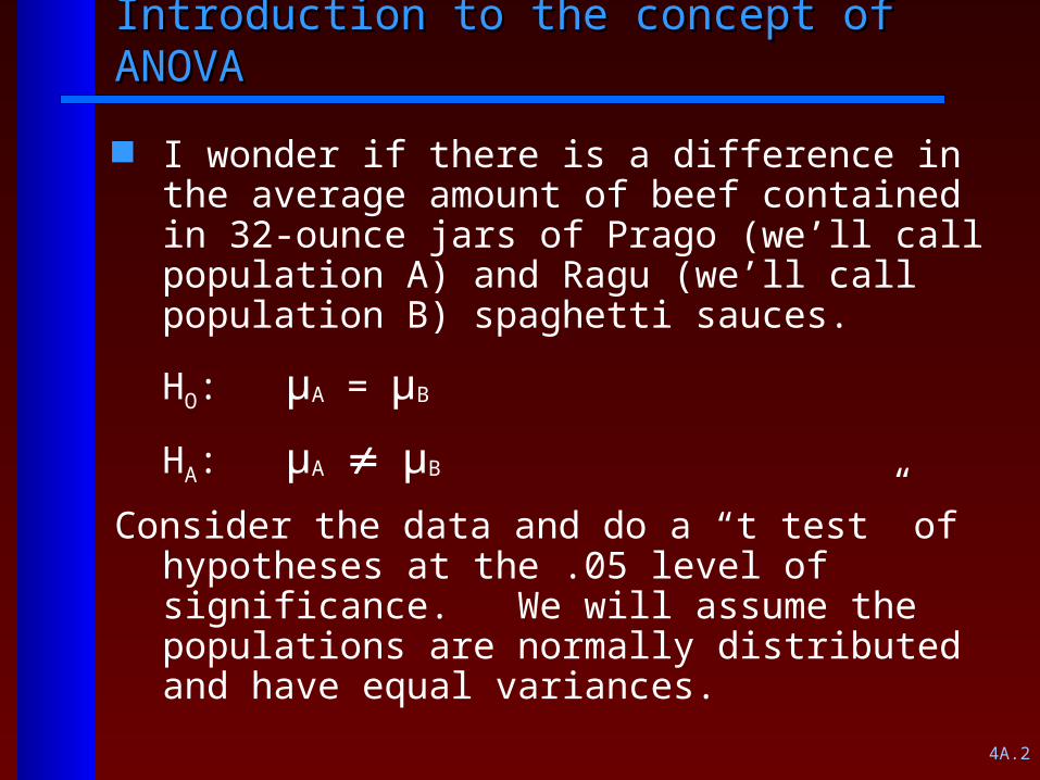
Introduction to the concept of ANOVAIntroduction to the concept of ANOVA

I wonder if there is a difference in the average amount of beef contained in 32-ounce jars of Prago (we’ll call population A) and Ragu (we’ll call population B) spaghetti sauces.

HO: µA = µB

HA: µA µB

Consider the data and do a “t test” of hypotheses at the .05 level of significance. We will assume the populations are normally distributed and have equal variances.

4A.3

A note on two-sample t tests . . .A note on two-sample t tests . . .

The degrees of freedom for a one-sample problem is n – 1, as you know.

The degrees of freedom for a two-sample problem is

n1 – 1 + n2 – 1 or n1 + n2 – 2

In the spaghetti sauce problem, the two sample t test the degrees of freedom would be 5 + 6 – 2 = 9

4A.4

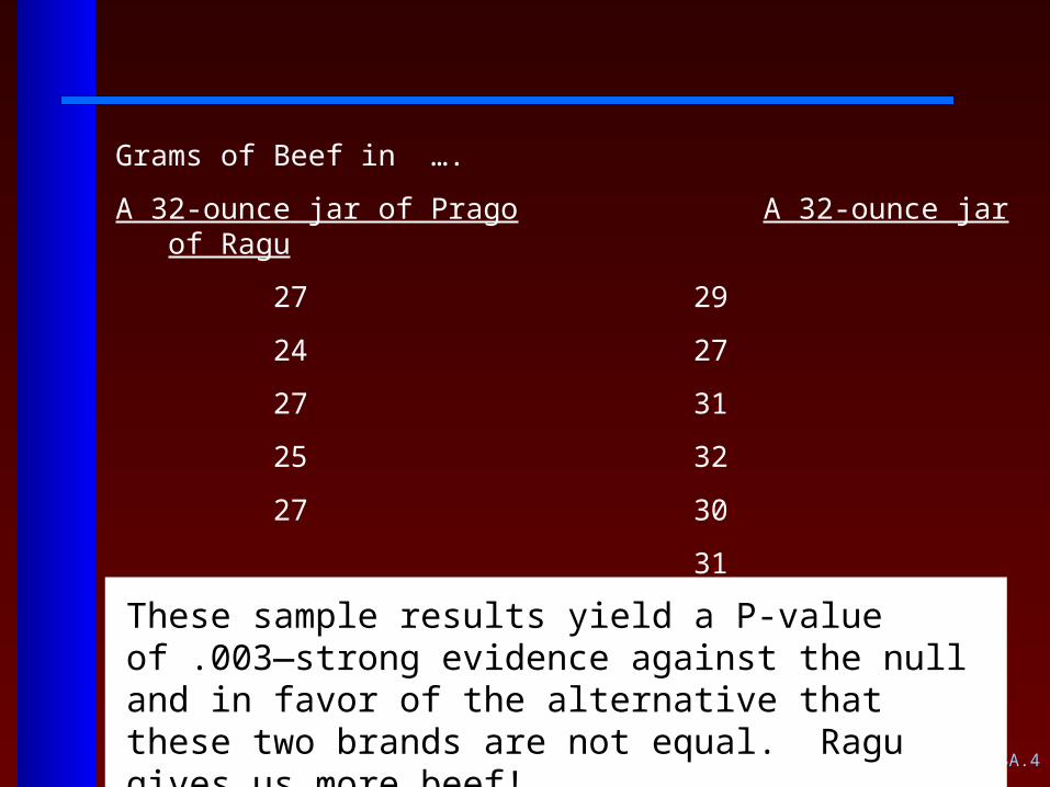
Grams of Beef in ….

A 32-ounce jar of Prago A 32-ounce jar of Ragu

27 29

24 27

27 31

25 32

27 30

31

These sample results yield a P-value of .003—strong evidence against the null and in favor of the alternative that these two brands are not equal. Ragu gives us more beef!

4A.5

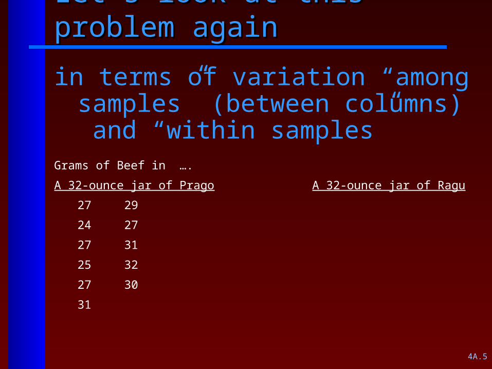
Let’s look at this problem againLet’s look at this problem again

in terms of variation “among samples” (between columns) and “within samples”

Grams of Beef in ….

A 32-ounce jar of Prago A 32-ounce jar of Ragu

27 29

24 27

27 31

25 32

27 30

31

4A.6

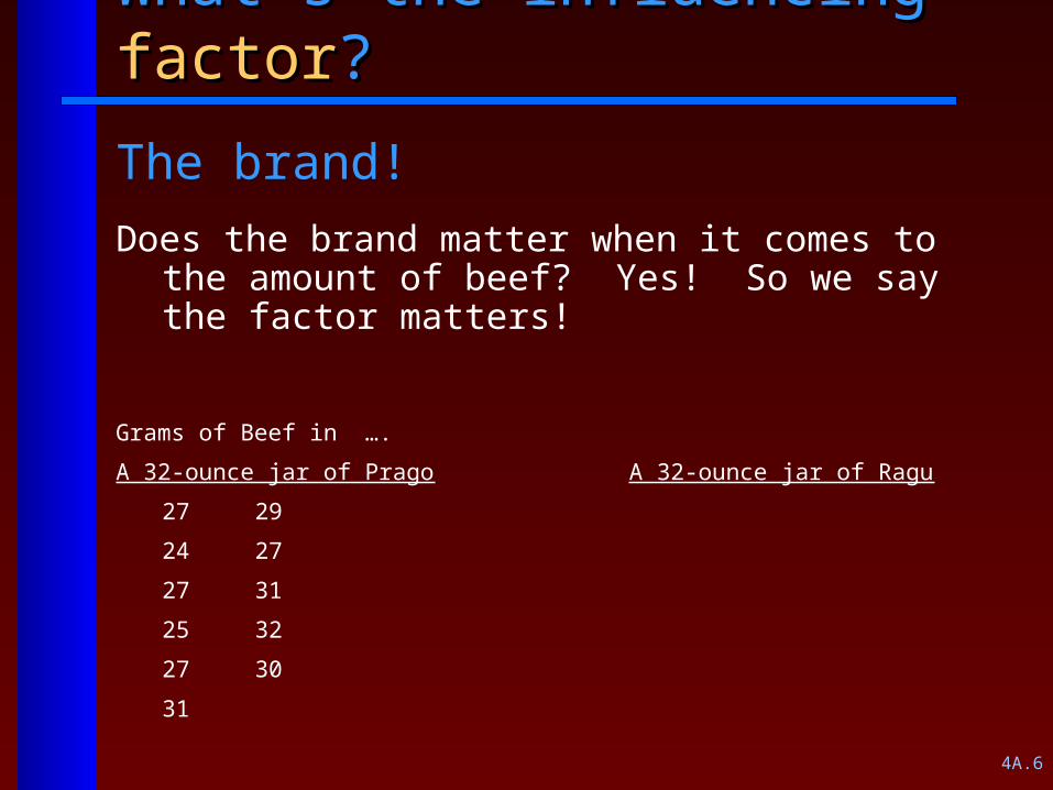
What’s the influencing What’s the influencing factorfactor??

The brand!

Does the brand matter when it comes to the amount of beef? Yes! So we say the factor matters!

Grams of Beef in ….

A 32-ounce jar of Prago A 32-ounce jar of Ragu

27 29

24 27

27 31

25 32

27 30

31

4A.7

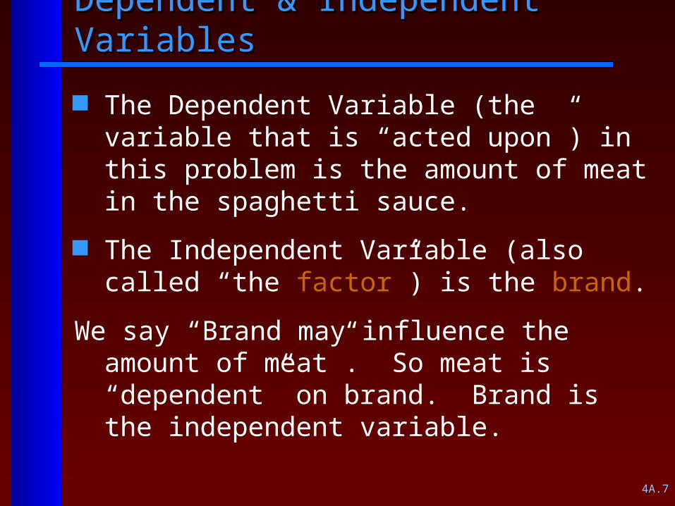
Dependent & Independent VariablesDependent & Independent Variables

The Dependent Variable (the variable that is “acted upon”) in this problem is the amount of meat in the spaghetti sauce.

The Independent Variable (also called “the factor”) is the brand.

We say “Brand may influence the amount of meat”. So meat is “dependent” on brand. Brand is the independent variable.

4A.8

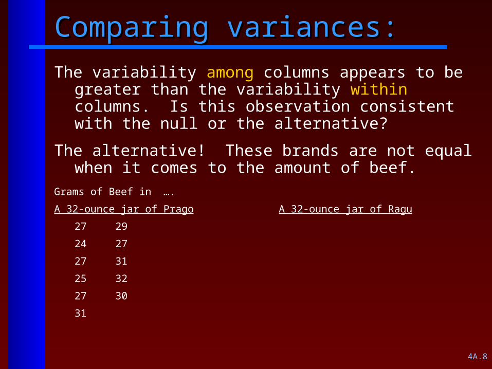
Comparing variances:Comparing variances:

The variability among columns appears to be greater than the variability within columns. Is this observation consistent with the null or the alternative?

The alternative! These brands are not equal when it comes to the amount of beef.

Grams of Beef in ….

A 32-ounce jar of Prago A 32-ounce jar of Ragu

27 29

24 27

27 31

25 32

27 30

31

4A.9

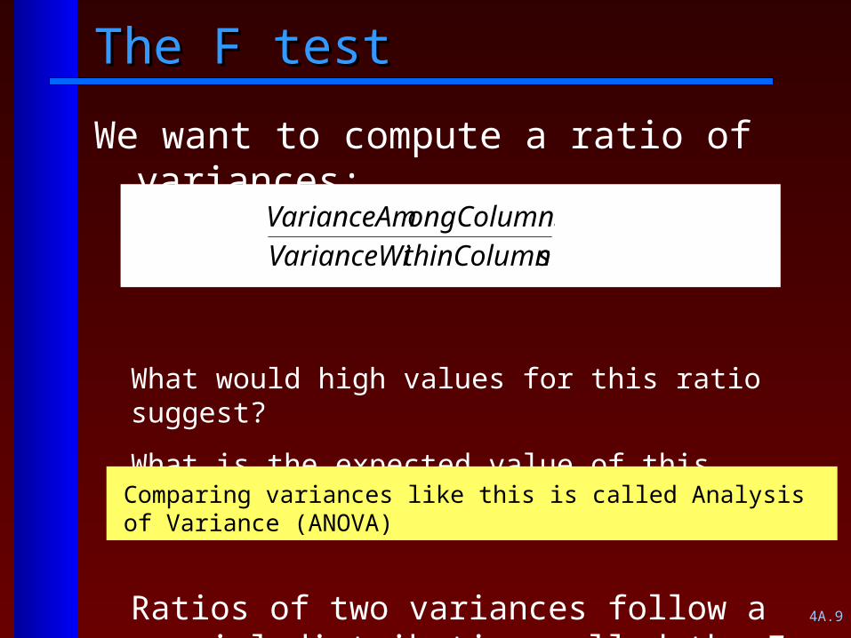
The F testThe F test

We want to compute a ratio of variances:

sthinColumnVarianceWiongColumnsVarianceAm

What would high values for this ratio suggest?

What is the expected value of this ratio if the null is true?

Ratios of two variances follow a special distribution called the F Distribution.

Comparing variances like this is called Analysis of Variance (ANOVA)

4A.10

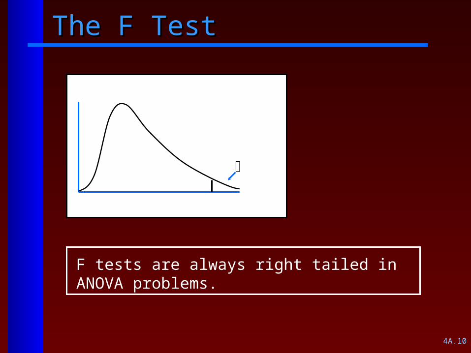
The F TestThe F Test

F tests are always right tailed in ANOVA problems.

4A.11

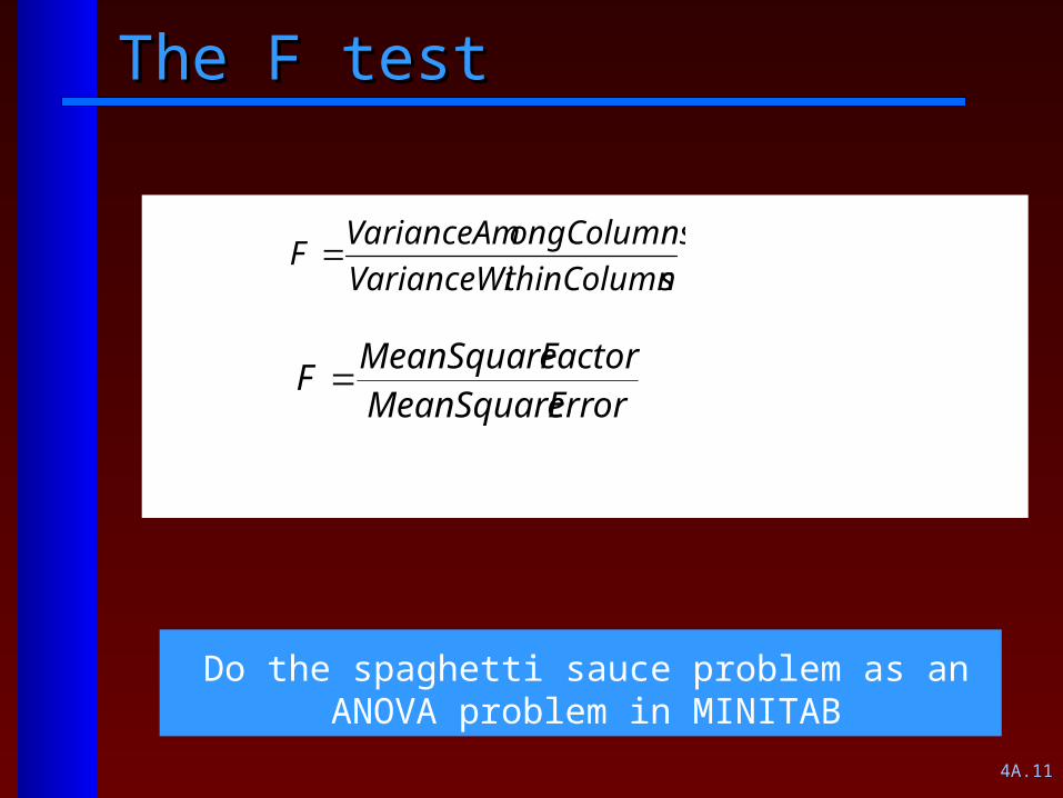
The F testThe F test

sthinColumnVarianceWi

ongColumnsVarianceAmF

ErrorMeanSquareFactorMeanSquare

F

Do the spaghetti sauce problem as an ANOVA problem in MINITAB

4A.12

Spaghetti Sauce ProblemSpaghetti Sauce Problem

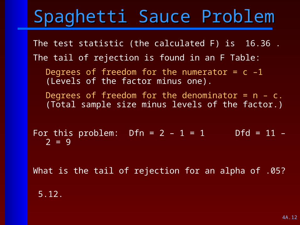
The test statistic (the calculated F) is 16.36 .

The tail of rejection is found in an F Table:

Degrees of freedom for the numerator = c –1 (Levels of the factor minus one).

Degrees of freedom for the denominator = n – c. (Total sample size minus levels of the factor.)

For this problem: Dfn = 2 – 1 = 1 Dfd = 11 – 2 = 9

What is the tail of rejection for an alpha of .05?

5.12.

4A.13

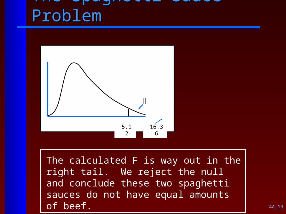
The Spaghetti Sauce ProblemThe Spaghetti Sauce Problem

The calculated F is way out in the right tail. We reject the null and conclude these two spaghetti sauces do not have equal amounts of beef.

5.12 16.36

4A.14

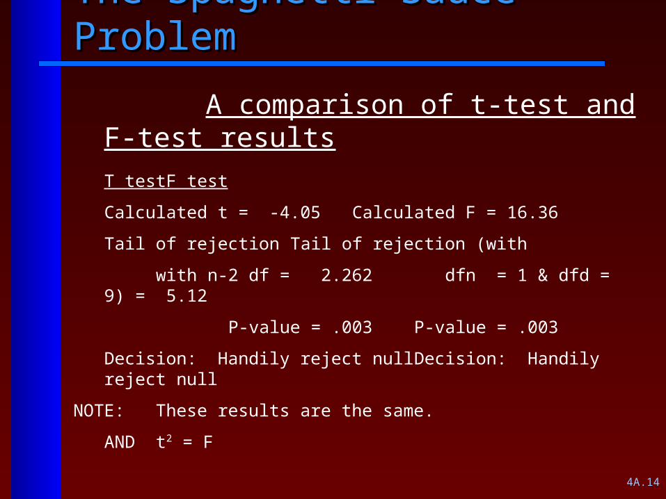
The Spaghetti Sauce ProblemThe Spaghetti Sauce Problem

A comparison of t-test and F-test results

T test F test

Calculated t = -4.05 Calculated F = 16.36

Tail of rejection Tail of rejection (with

with n-2 df = 2.262 dfn = 1 & dfd = 9) = 5.12

P-value = .003 P-value = .003

Decision: Handily reject null Decision: Handily reject null

NOTE: These results are the same.

AND t2 = F

4A.15

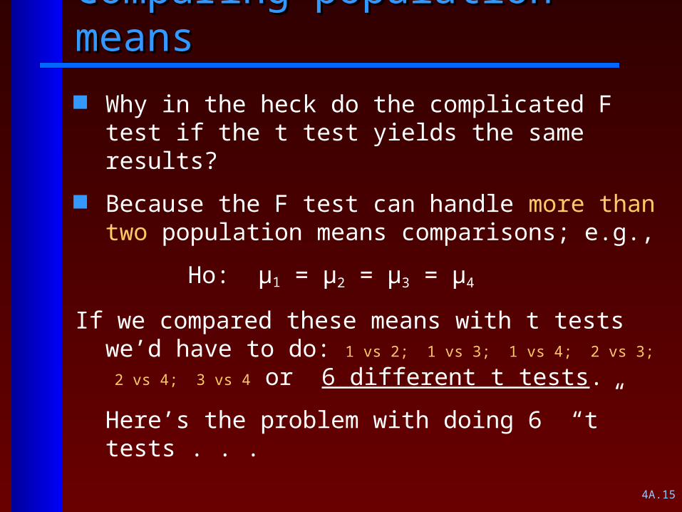
Comparing population meansComparing population means

Why in the heck do the complicated F test if the t test yields the same results?

Because the F test can handle more than two population means comparisons; e.g.,

Ho: µ1 = µ2 = µ3 = µ4

If we compared these means with t tests we’d have to do: 1 vs 2; 1 vs 3; 1 vs 4; 2 vs 3; 2 vs 4; 3 vs 4 or 6 different t tests.

Here’s the problem with doing 6 “t” tests . . .

4A.16

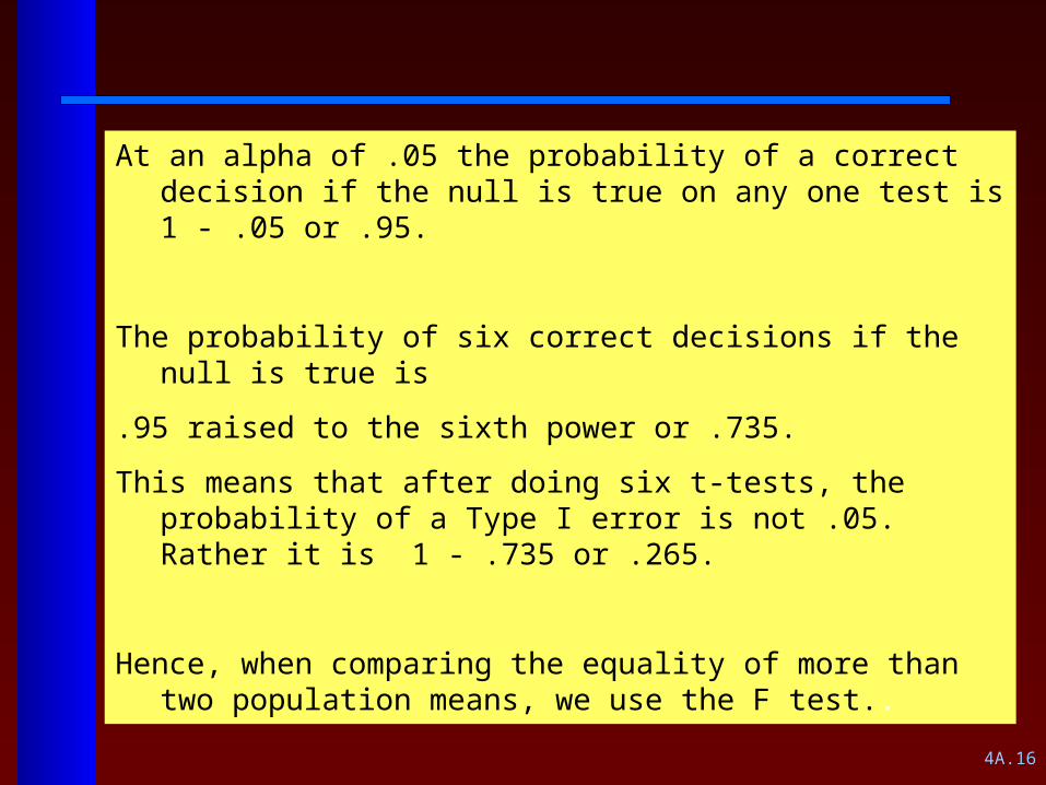
At an alpha of .05 the probability of a correct decision if the null is true on any one test is 1 - .05 or .95.

The probability of six correct decisions if the null is true is

.95 raised to the sixth power or .735.

This means that after doing six t-tests, the probability of a Type I error is not .05. Rather it is 1 - .735 or .265.

Hence, when comparing the equality of more than two population means, we use the F test..

4A.17

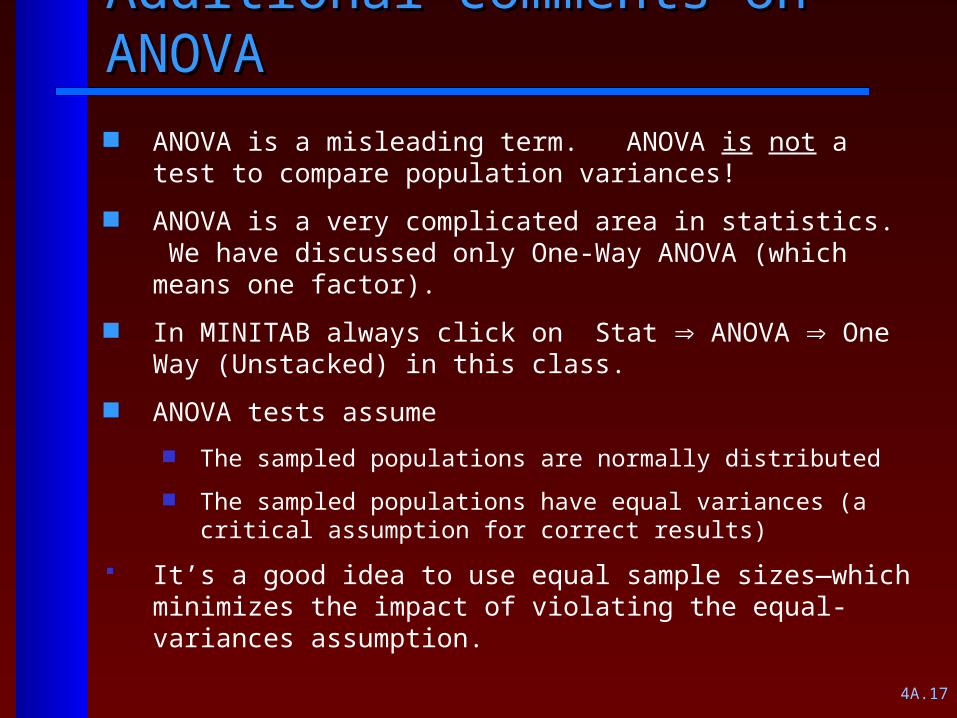
Additional comments on ANOVAAdditional comments on ANOVA ANOVA is a misleading term. ANOVA is not a test to compare

population variances!

ANOVA is a very complicated area in statistics. We have discussed only One-Way ANOVA (which means one factor).

In MINITAB always click on Stat ANOVA One Way (Unstacked) in this class.

ANOVA tests assume

The sampled populations are normally distributed

The sampled populations have equal variances (a critical assumption for correct results)

It’s a good idea to use equal sample sizes—which minimizes the impact of violating the equal-variances assumption.

4A.18

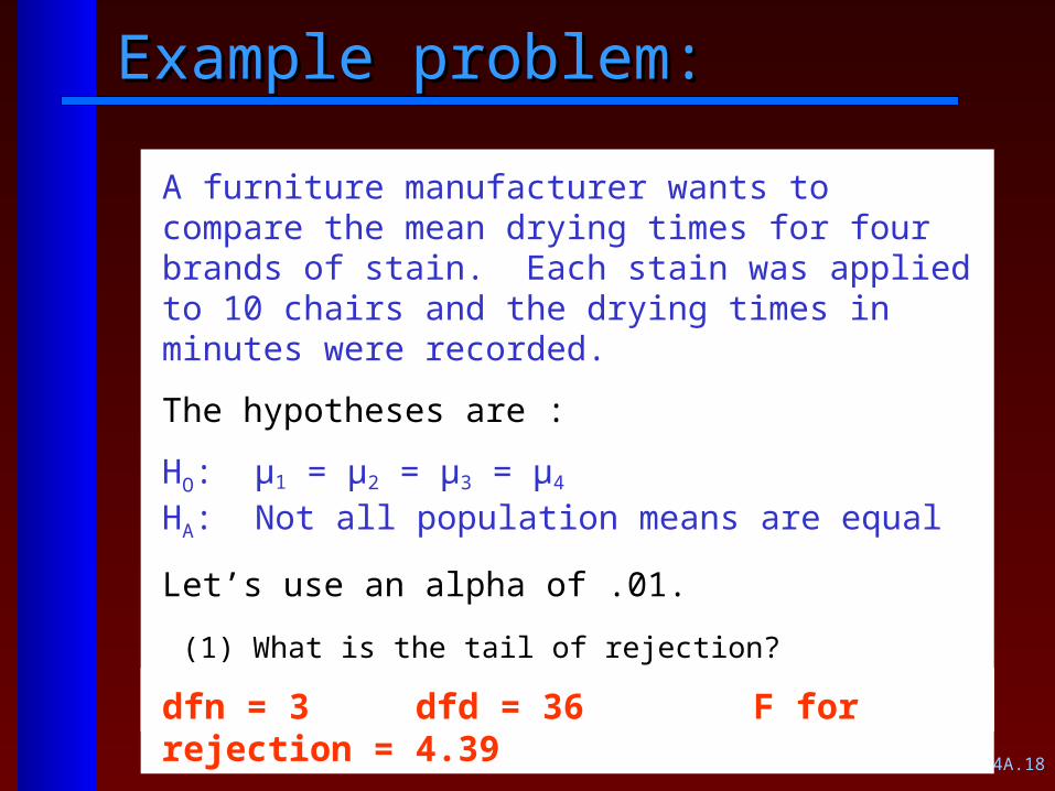
Example problem:Example problem:

A furniture manufacturer wants to compare the mean drying times for four brands of stain. Each stain was applied to 10 chairs and the drying times in minutes were recorded.

The hypotheses are :

HO: µ1 = µ2 = µ3 = µ4

HA: Not all population means are equal

Let’s use an alpha of .01.

(1) What is the tail of rejection?

(2) Solve the problem with MINITAB

dfn = 3 dfd = 36 F for rejection = 4.39

4A.19

Homework Assignment for ANOVAHomework Assignment for ANOVA

Problem Set 4

4A.20

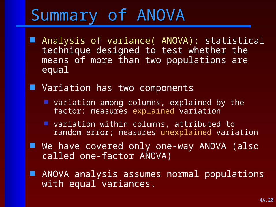
Summary of ANOVA Summary of ANOVA Analysis of variance( ANOVA): statistical technique

designed to test whether the means of more than two populations are equal

Variation has two components

variation among columns, explained by the factor: measures explained variation

variation within columns, attributed to random error; measures unexplained variation

We have covered only one-way ANOVA (also called one-factor ANOVA)

ANOVA analysis assumes normal populations with equal variances.

4A.21

Homework solutions:Homework solutions:

1. HO: L = M = H

HA: Not all of the population means are equal

dfn = c – 1 = 2 dfd = n – c = 12

The Tail of Rejection in a F distribution is defined as 5.10 for 2.5 percent level of significance.

The F statistic is 1.92, which means the variability attributable to levels of the factor is 1.92 times greater than the random variability.

P-Value is .189, which is interpreted as: “If the Null is true, there is a .189 chance of observing an F statistic as contradictory (or more contradictory) to the null as the value found here.”

We fail to reject the null. We do not have sufficiently strong evidence to run with the conclusion that housing prices are not the same for three areas with different levels of air pollution.

4A.22

Homework solutions:Homework solutions:

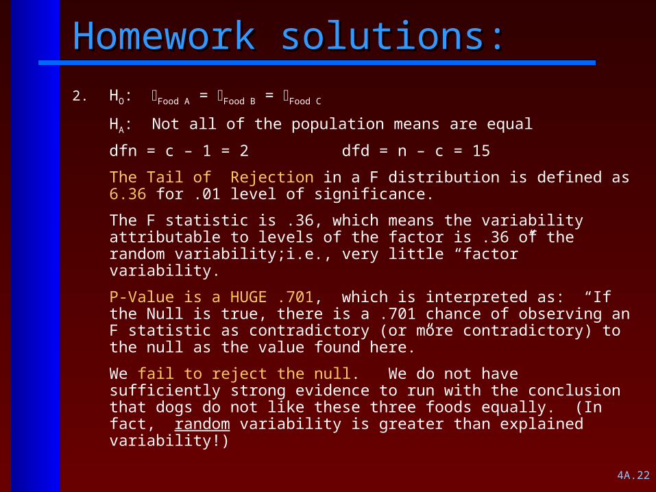
2. HO: Food A = Food B = Food C

HA: Not all of the population means are equal

dfn = c – 1 = 2 dfd = n – c = 15

The Tail of Rejection in a F distribution is defined as 6.36 for .01 level of significance.

The F statistic is .36, which means the variability attributable to levels of the factor is .36 of the random variability;i.e., very little “factor” variability.

P-Value is a HUGE .701, which is interpreted as: “If the Null is true, there is a .701 chance of observing an F statistic as contradictory (or more contradictory) to the null as the value found here.”

We fail to reject the null. We do not have sufficiently strong evidence to run with the conclusion that dogs do not like these three foods equally. (In fact, random variability is greater than explained variability!)

4A.23

Homework solutions:Homework solutions:

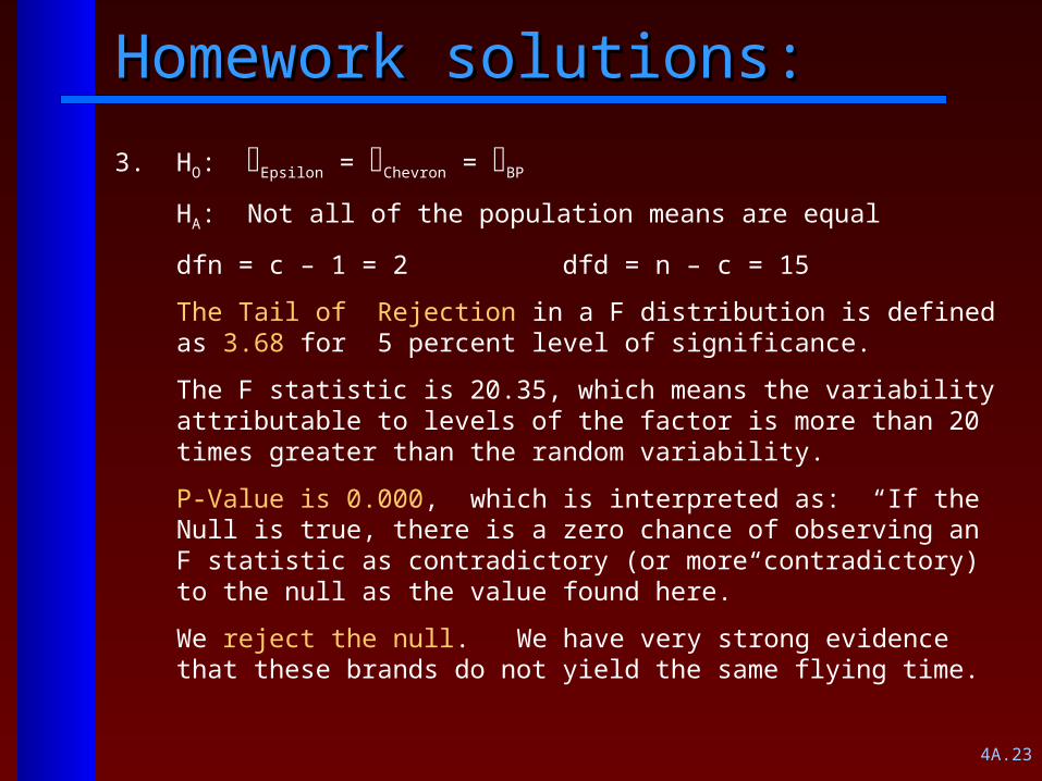
3. HO: Epsilon = Chevron = BP

HA: Not all of the population means are equal

dfn = c – 1 = 2 dfd = n – c = 15

The Tail of Rejection in a F distribution is defined as 3.68 for 5 percent level of significance.

The F statistic is 20.35, which means the variability attributable to levels of the factor is more than 20 times greater than the random variability.

P-Value is 0.000, which is interpreted as: “If the Null is true, there is a zero chance of observing an F statistic as contradictory (or more contradictory) to the null as the value found here.”

We reject the null. We have very strong evidence that these brands do not yield the same flying time.