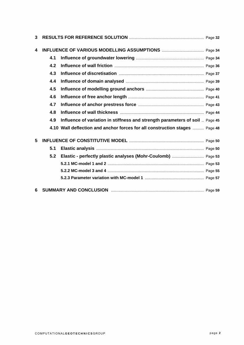
PART I: RESULTS OF BENCHMARKING PART II: REFERENCE ...2002...PART I: RESULTS OF BENCHMARKING PART II: REFERENCE SOLUTION AND PARAMETRIC STUDY March 2002 / CGG_IR006_2002 BENCHMARKING

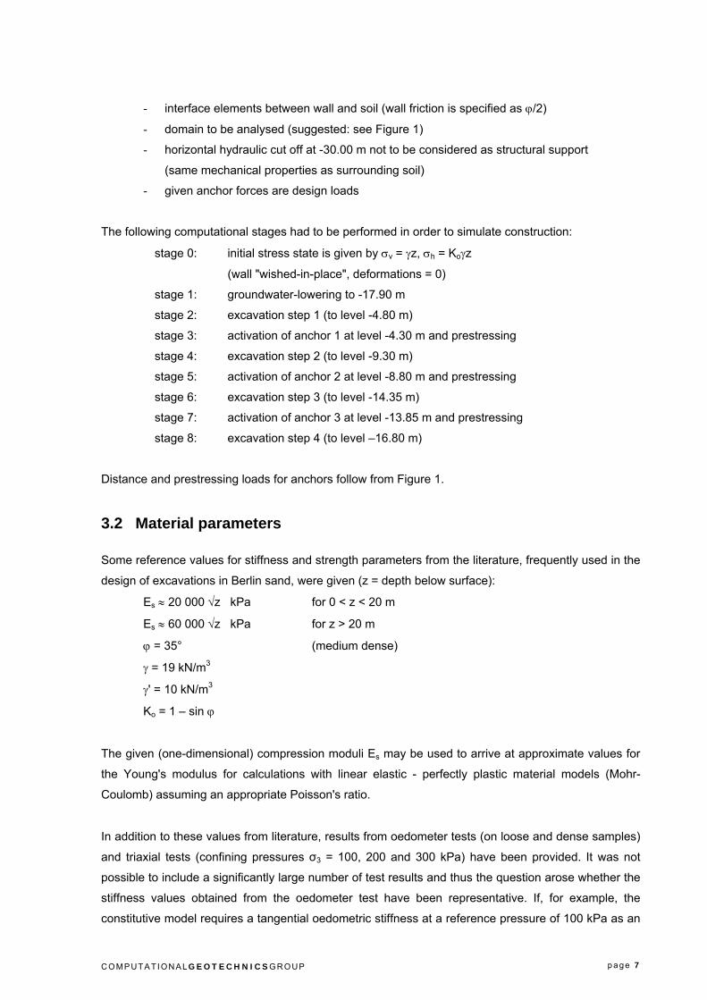
PART I: RESULTS OF BENCHMARKINGPART II: REFERENCE SOLUTION AND PARAMETRIC STUDY

/ CGG_IR006_2002March 2002

BENCHMARKING IN GEOTECHNICS_1

Helmut F. Schweiger

Institute for Soil Mechanics and Foundation Engineering

Graz University of Technology, Austria

horizontal displacement [mm]

-70 -65 -60 -55 -50 -45 -40 -35 -30 -25 -20 -15 -10 -5 0

-70 -65 -60 -55 -50 -45 -40 -35 -30 -25 -20 -15 -10 -5 0

de

pth

be

low

su

rfa

ce

[m]

0

2

4

6

8

10

12

14

16

18

20

22

24

26

28

30

32

reference solutionR

inter= 0.8 (final stage)

Rinter

= 0.5 (final stage)

Rinter

= 0.8 t_virt = 0.01

(final stage)

reference solution(1. excavation stage)

Rinter

= 0.5

(1. excavation stage)

Rinter

= 0.8 t_virt = 0.01

(1. excavation stage)

distance from wall [m]

0 10 20 30 40 50 60 70 80 90 100

-30

-25

-20

-15

-10

-5

0

5

10

reference solution

anchor -4m

anchor +8m

C O M P UT A TI O N A LGEOTECHNICSG R O UP p a ge 1

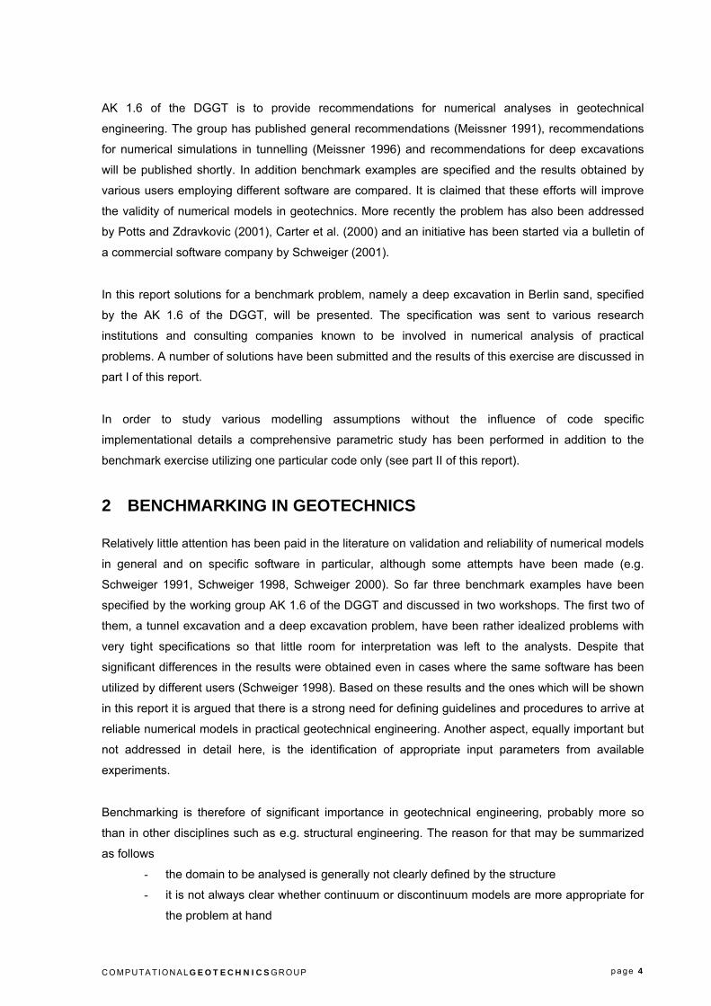
CONTENTS PART I: RESULTS OF BENCHMARKING

ABSTRACT ................................................................................................................................ Page 3

1 INTRODUCTION ................................................................................................................. Page 3

2 BENCHMARKING IN GEOTECHNICS ......................................................................... Page 4

3 PROBLEM SPECIFICATION: DEEP EXCAVATION IN BERLIN SAND ................ Page 5 3.1 Assumptions and geometry .......................................................................... Page 5 3.2 Material parameters ......................................................................................... Page 7

4 COMMENTS ON SUBMITTED SOLUTIONS ............................................................... Page 8

5 COMPARISON OF RESULTS ...................................................................................... Page 11 5.1 Comparison of all analyses submitted ..................................................... Page 11 5.2 Comparison of selected results ................................................................. Page 13

5.2.1 Construction stage groundwater lowering to -17.90 m ........................ Page 13

5.2.2 Construction stage first excavation step to -4.80 m.............................. Page 14

5.2.3 Final construction stage .......................................................................... Page 16 5.3 Comparison elastic-plastic vs. elastic-perfectly plastic analyses .... Page 20

6 SUMMARY AND CONCLUSION .................................................................................. Page 24

7 REFERENCES ................................................................................................................. Page 24

PART II: REFERENCE SOLUTION AND PARAMETRIC STUDY

ABSTRACT .............................................................................................................................. Page 26

1 INTRODUCTION ............................................................................................................... Page 26

2 PROBLEM DEFINITION ................................................................................................. Page 27 2.1 Geometry, basic assumptions and computational steps .................... Page 27

2.2 Brief description of PLAXIS Hardening Soil model................................ Page 29 2.3 Material parameters for Hardening Soil model ....................................... Page 31

2.4 Material parameters for structural elements .......................................... Page 31


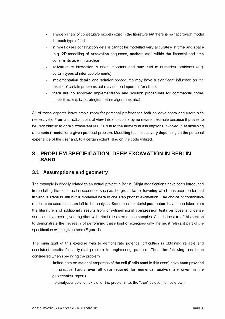
3 RESULTS FOR REFERENCE SOLUTION .................................................................. Page 32

4 INFLUENCE OF VARIOUS MODELLING ASSUMPTIONS ..................................... Page 34 4.1 Influence of groundwater lowering ............................................................ Page 34 4.2 Influence of wall friction ............................................................................... Page 36 4.3 Influence of discretisation ........................................................................... Page 37 4.4 Influence of domain analysed ..................................................................... Page 39

4.5 Influence of modelling ground anchors ................................................... Page 40

4.6 Influence of free anchor length ................................................................... Page 41

4.7 Influence of anchor prestress force .......................................................... Page 43

4.8 Influence of wall thickness .......................................................................... Page 44

4.9 Influence of variation in stiffness and strength parameters of soil .. Page 45

4.10 Wall deflection and anchor forces for all construction stages .......... Page 48

5 INFLUENCE OF CONSTITUTIVE MODEL .................................................................. Page 50 5.1 Elastic analysis ............................................................................................... Page 50 5.2 Elastic - perfectly plastic analyses (Mohr-Coulomb) ............................ Page 53

5.2.1 MC-model 1 and 2 ..................................................................................... Page 53

5.2.2 MC-model 3 and 4 ..................................................................................... Page 55

5.2.3 Parameter variation with MC-model 1 .................................................... Page 57

6 SUMMARY AND CONCLUSION .................................................................................. Page 59


PART I: RESULTS OF BENCHMARKING ABSTRACT

In part I of this report the results of a benchmarking exercise are presented. A deep excavation

problem in Berlin sand has been specified by the working AK 1.6 of the German Society for

Geotechnics and sent to various university institutes and consulting companies known to deal with

numerical analysis in practical geotechnical engineering. The results summarized in this report clearly

emphasize the need for these types of exercises in order to improve the reliability and validity of

numerical models. The wide range of results submitted is by no means acceptable and therefore it is

argued that guidelines and recommendations have to be formulated in order to assist numerical

analysts in avoiding unrealistic modelling assumptions, which may lead to consequences the user of a

particular code may not be aware of.

1 INTRODUCTION

The significant progress made in the understanding of the behaviour of geomaterials would not have

been possible without the use of numerical methods. In particular, developments in constitutive

modelling are closely related to advances made in the field of numerical analysis and therefore finite

element (and other) methods have had a significant impact on geotechnical research since the 1970s.

However, numerical methods have not been widely used in practical geotechnical engineering,

possibly with a few exceptions, such as tunnelling, where these methods have a long tradition also in

practice, at least in some parts of the world. But this has changed dramatically over the last decade.

Developments in computer hardware and, more importantly, in geotechnical software enable the

geotechnical engineer to perform very advanced numerical analyses at low cost and with relatively

little computational effort. Commercial codes, fully integrated into the PC-environment, have become

so user-friendly that little training is required for operating the programme. They offer sophisticated

types of analysis, such as fully coupled consolidation analysis with elasto-plastic material models.

However, for performing such complex calculations and obtaining sensible results a strong

background in numerical methods, mechanics and, last but not least, theoretical soil mechanics is

essential. This is sometimes overlooked in practice because glossy brochures give the impression that

achieving reliable results is as easy as operating the programme and this is certainly not true.

The potential problems arising from the situation that geotechnical engineers, not sufficiently trained

for that purpose, perform complex numerical analyses and may produce unreliable results have been

recognized within the profession and some national and international committees have begun to

address this problem, amongst them the working group AK 1.6 "Numerical Methods in Geotechnics" of

the German Society for Geotechnics (DGGT) and working group A "Numerical Methods" of the COST

Action C7 (Co-Operation in Science and Technology of the European Union). One of the main goals of


AK 1.6 of the DGGT is to provide recommendations for numerical analyses in geotechnical

engineering. The group has published general recommendations (Meissner 1991), recommendations

for numerical simulations in tunnelling (Meissner 1996) and recommendations for deep excavations

will be published shortly. In addition benchmark examples are specified and the results obtained by

various users employing different software are compared. It is claimed that these efforts will improve

the validity of numerical models in geotechnics. More recently the problem has also been addressed

by Potts and Zdravkovic (2001), Carter et al. (2000) and an initiative has been started via a bulletin of

a commercial software company by Schweiger (2001).

In this report solutions for a benchmark problem, namely a deep excavation in Berlin sand, specified

by the AK 1.6 of the DGGT, will be presented. The specification was sent to various research

institutions and consulting companies known to be involved in numerical analysis of practical

problems. A number of solutions have been submitted and the results of this exercise are discussed in

part I of this report.

In order to study various modelling assumptions without the influence of code specific

implementational details a comprehensive parametric study has been performed in addition to the

benchmark exercise utilizing one particular code only (see part II of this report).

2 BENCHMARKING IN GEOTECHNICS

Relatively little attention has been paid in the literature on validation and reliability of numerical models

in general and on specific software in particular, although some attempts have been made (e.g.

Schweiger 1991, Schweiger 1998, Schweiger 2000). So far three benchmark examples have been

specified by the working group AK 1.6 of the DGGT and discussed in two workshops. The first two of

them, a tunnel excavation and a deep excavation problem, have been rather idealized problems with

very tight specifications so that little room for interpretation was left to the analysts. Despite that

significant differences in the results were obtained even in cases where the same software has been

utilized by different users (Schweiger 1998). Based on these results and the ones which will be shown

in this report it is argued that there is a strong need for defining guidelines and procedures to arrive at

reliable numerical models in practical geotechnical engineering. Another aspect, equally important but

not addressed in detail here, is the identification of appropriate input parameters from available

experiments.

Benchmarking is therefore of significant importance in geotechnical engineering, probably more so

than in other disciplines such as e.g. structural engineering. The reason for that may be summarized

as follows

- the domain to be analysed is generally not clearly defined by the structure

- it is not always clear whether continuum or discontinuum models are more appropriate for

the problem at hand


- a wide variety of constitutive models exist in the literature but there is no "approved" model

for each type of soil

- in most cases construction details cannot be modelled very accurately in time and space

(e.g. 2D-modelling of excavation sequence, anchors etc.) within the financial and time

constraints given in practice

- soil/structure interaction is often important and may lead to numerical problems (e.g.

certain types of interface elements)

- implementation details and solution procedures may have a significant influence on the

results of certain problems but may not be important for others

- there are no approved implementation and solution procedures for commercial codes

(implicit vs. explicit strategies, return algorithms etc.)

All of these aspects leave ample room for personal preferences both on developers and users side

respectively. From a practical point of view this situation is by no means desirable because it proves to

be very difficult to obtain consistent results due to the numerous assumptions involved in establishing

a numerical model for a given practical problem. Modelling techniques vary depending on the personal

experience of the user and, to a certain extent, also on the code utilized.

3 PROBLEM SPECIFICATION: DEEP EXCAVATION IN BERLIN SAND

3.1 Assumptions and geometry

The example is closely related to an actual project in Berlin. Slight modifications have been introduced

in modelling the construction sequence such as the groundwater lowering which has been performed

in various steps in situ but is modelled here in one step prior to excavation. The choice of constitutive

model to be used has been left to the analysts. Some basic material parameters have been taken from

the literature and additionally results from one-dimensional compression tests on loose and dense

samples have been given together with triaxial tests on dense samples. As it is the aim of this section

to demonstrate the necessity of performing these kind of exercises only the most relevant part of the

specification will be given here (Figure 1).

The main goal of this exercise was to demonstrate potential difficulties in obtaining reliable and

consistent results for a typical problem in engineering practice. Thus the following has been

considered when specifying the problem:

- limited data on material properties of the soil (Berlin sand in this case) have been provided

(in practice hardly ever all data required for numerical analysis are given in the

geotechnical report)

- no analytical solution exists for the problem, i.e. the "true" solution is not known


- the problem is related to a project actually constructed, so the order of magnitude of

horizontal displacements of the wall is known from in situ measurements

- no restraints are imposed with respect to the constitutive model, discretisation, element

types etc.

Thus the benchmarking exercise did not aim at the verification of particular software packages for

solving a problem with a known solution but to see what range of numerical solutions for a

geotechnical problem can be expected under conditions typically found in practice. For these reasons

neither programme names nor authors of solutions submitted are disclosed in this report (they are

denoted by B1 to B17 throughout this report).

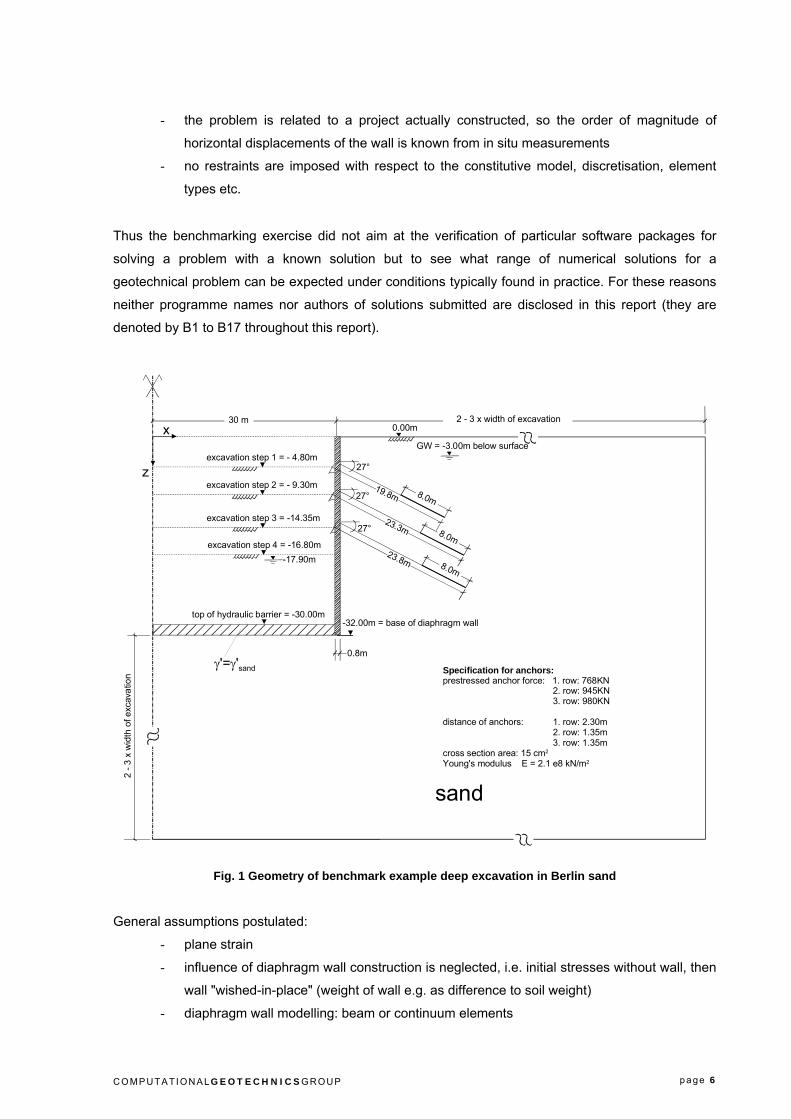
Fig. 1 Geometry of benchmark example deep excavation in Berlin sand

General assumptions postulated:

- plane strain

- influence of diaphragm wall construction is neglected, i.e. initial stresses without wall, then

wall "wished-in-place" (weight of wall e.g. as difference to soil weight)

- diaphragm wall modelling: beam or continuum elements

23.3m

8.0m

8.0m

19.8m

27°

27°

0.8m

-32.00m = base of diaphragm wall

excavation step 3 = -14.35m

GW = -3.00m below surface

0.00m

excavation step 2 = - 9.30m

excavation step 1 = - 4.80m

30 m

Specification for anchors:prestressed anchor force: 1. row: 768KN 2. row: 945KN 3. row: 980KN

distance of anchors: 1. row: 2.30m 2. row: 1.35m 3. row: 1.35mcross section area: 15 cm2

Young's modulus E = 2.1 e8 kN/m2

top of hydraulic barrier = -30.00m

excavation step 4 = -16.80m-17.90m 23.8m 8.0m

27°

2 - 3 x width of excavation

2 - 3

x w

idth

of e

xcav

atio

n

sand

γ'=γ'sand

x

z


- interface elements between wall and soil (wall friction is specified as ϕ/2)

- domain to be analysed (suggested: see Figure 1)

- horizontal hydraulic cut off at -30.00 m not to be considered as structural support

(same mechanical properties as surrounding soil)

- given anchor forces are design loads

The following computational stages had to be performed in order to simulate construction:

stage 0: initial stress state is given by σv = γz, σh = Koγz

(wall "wished-in-place", deformations = 0)

stage 1: groundwater-lowering to -17.90 m

stage 2: excavation step 1 (to level -4.80 m)

stage 3: activation of anchor 1 at level -4.30 m and prestressing





stage 8: excavation step 4 (to level –16.80 m)

Distance and prestressing loads for anchors follow from Figure 1.

3.2 Material parameters

Some reference values for stiffness and strength parameters from the literature, frequently used in the

design of excavations in Berlin sand, were given (z = depth below surface):

Es ≈ 20 000 √z kPa for 0 < z < 20 m

Es ≈ 60 000 √z kPa for z > 20 m

ϕ = 35° (medium dense)

γ = 19 kN/m3

γ' = 10 kN/m3

Ko = 1 – sin ϕ

The given (one-dimensional) compression moduli Es may be used to arrive at approximate values for

the Young's modulus for calculations with linear elastic - perfectly plastic material models (Mohr-

Coulomb) assuming an appropriate Poisson's ratio.

In addition to these values from literature, results from oedometer tests (on loose and dense samples)

and triaxial tests (confining pressures σ3 = 100, 200 and 300 kPa) have been provided. It was not

possible to include a significantly large number of test results and thus the question arose whether the

stiffness values obtained from the oedometer test have been representative. If, for example, the

constitutive model requires a tangential oedometric stiffness at a reference pressure of 100 kPa as an


input parameter, a value of only Es ≈ 12 000 kPa was found based on these experiments. If a secant

modulus for a pressure range beyond 200 kPa is determined a value of about 40 000 kPa is obtained.

This was considered as too low by many authors and indeed other test results from Berlin sand in the

literature indicate higher values. For example from Ohde (1951) values of about 35 000 to 45 000 kPa

could be estimated as reference loading modulus of a medium dense sand at a reference pressure of

100 kPa. However, sample disturbance and uncertainties in laboratory testing cannot be neglected, at

least not in standard procedures usually performed for practical purposes, and therefore it has to be

carefully judged whether stiffness values obtained in the laboratory should be used in numerical

analysis without correction. These problems of determining appropriate stiffness parameters for

numerical analyses are by no means desirable, but unfortunately it represents the situation in practice

where geotechnical investigations and geotechnical reports often do not satisfy the requirements for

numerical analysis. It can be anticipated however that more refined experimental investigations,

including the measurement of stiffness at very small strains, will be employed increasingly for practical

purposes and thus provide more reliable data for numerical analysis.

Properties for the diaphragm wall (linear elastic):

E = 30 000 x 103 kPa

ν = 0.15

γ = 24 kN/m3

4 COMMENTS ON SUBMITTED SOLUTIONS

A wide variety of programmes and constitutive models has been employed to solve this problem.

Simple elastic-perfectly plastic material models such as the Mohr-Coulomb or Drucker-Prager failure

functions (B1, B4, B5, B6, B7, B9, B12 and B16), still widely used in practice have been chosen by a

number of authors. Several entries utilized the computer code PLAXIS (Brinkgreve & Vermeer 1998)

with the so-called Hardening Soil model. This constitutive model is based on the well known

formulation by Duncan & Chang (1970), but formulated within the theory of plasticity. It incorporates

shear hardening and volumetric hardening, a stress dependent stiffness for primary loading and

unloading/reloading and the stress dilatancy theory by Rowe (1962). One submission used a similar

plasticity model with a simplified small strain stiffness formulation for the elastic range (B14). Three

entries employed a hypoplastic formulation (B3, B3a and B13), B3 without and B3a and B13 with

considering intergranular strains (Niemunis & Herle 1997).

Only marginal differences exist in the assumptions of strength parameters (everybody trusted the

experiments in this respect), the angle of internal friction ϕ was taken as 36° or 37° and a small

cohesion was assumed to increase numerical stability by some authors. A significant variation was

observed however in the assumption of the dilatancy angle ψ, ranging from 0° to 15°.


For reasons mentioned earlier only a limited number of analysts used the provided laboratory test

results to calibrate their material model. Most of the analysts used data from the literature from Berlin

sand or their own experience to arrive at input parameters for their analysis assuming an increase with

depth either by introducing some sort of power law similar to the formulation presented by Ohde

(1951) which in turn corresponds to the formulation by Janbu (1963), or by defining different layers

with different (constant) Young's moduli. However the choice of the reference moduli for primary

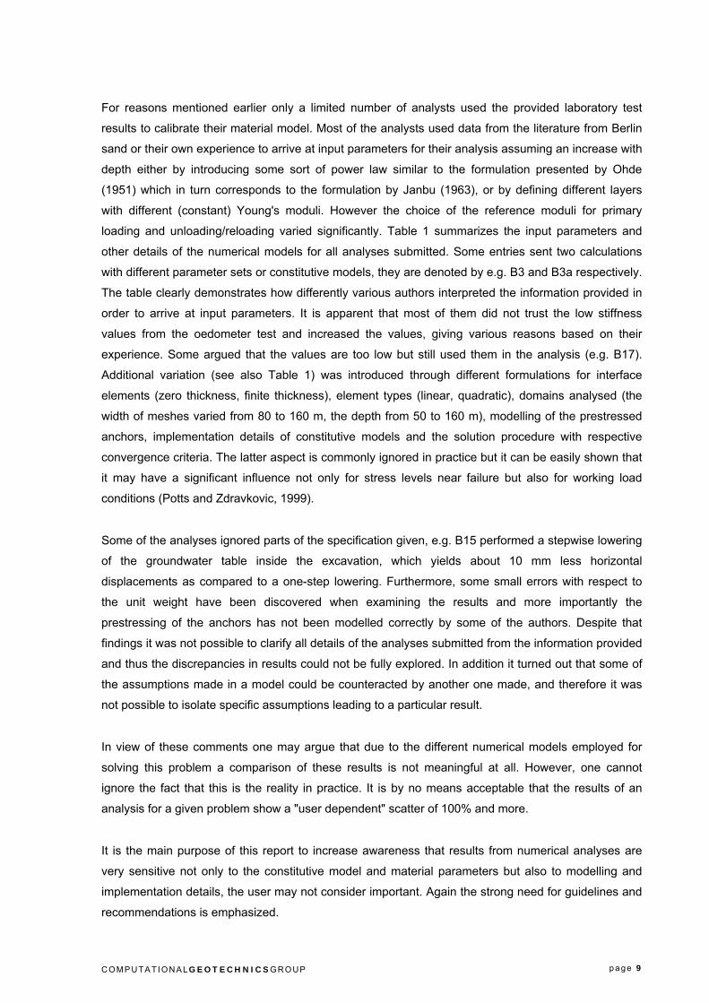
loading and unloading/reloading varied significantly. Table 1 summarizes the input parameters and

other details of the numerical models for all analyses submitted. Some entries sent two calculations

with different parameter sets or constitutive models, they are denoted by e.g. B3 and B3a respectively.

The table clearly demonstrates how differently various authors interpreted the information provided in

order to arrive at input parameters. It is apparent that most of them did not trust the low stiffness

values from the oedometer test and increased the values, giving various reasons based on their

experience. Some argued that the values are too low but still used them in the analysis (e.g. B17).

Additional variation (see also Table 1) was introduced through different formulations for interface

elements (zero thickness, finite thickness), element types (linear, quadratic), domains analysed (the

width of meshes varied from 80 to 160 m, the depth from 50 to 160 m), modelling of the prestressed

anchors, implementation details of constitutive models and the solution procedure with respective

convergence criteria. The latter aspect is commonly ignored in practice but it can be easily shown that

it may have a significant influence not only for stress levels near failure but also for working load

conditions (Potts and Zdravkovic, 1999).

Some of the analyses ignored parts of the specification given, e.g. B15 performed a stepwise lowering

of the groundwater table inside the excavation, which yields about 10 mm less horizontal

displacements as compared to a one-step lowering. Furthermore, some small errors with respect to

the unit weight have been discovered when examining the results and more importantly the

prestressing of the anchors has not been modelled correctly by some of the authors. Despite that

findings it was not possible to clarify all details of the analyses submitted from the information provided

and thus the discrepancies in results could not be fully explored. In addition it turned out that some of

the assumptions made in a model could be counteracted by another one made, and therefore it was

not possible to isolate specific assumptions leading to a particular result.

In view of these comments one may argue that due to the different numerical models employed for

solving this problem a comparison of these results is not meaningful at all. However, one cannot

ignore the fact that this is the reality in practice. It is by no means acceptable that the results of an

analysis for a given problem show a "user dependent" scatter of 100% and more.

It is the main purpose of this report to increase awareness that results from numerical analyses are

very sensitive not only to the constitutive model and material parameters but also to modelling and

implementation details, the user may not consider important. Again the strong need for guidelines and

recommendations is emphasized.


Table 1 Summary of all analyses submitted

analysis constitutive model stiffness reference stiffness

(loading / unloading) [kPa]

n

[o]

R

[o]

domain analysedwidth x depth [m]

element typesoil

element type wall

interface note

B1 elastic-perfectly plastic stress dependent z < 20 m: 14 900

z > 20 m: 44 700 35 5 100 x 64 quadratic

9 noded

continuum yes -

B2 / B2a elastic-plastic (z < 40 m)

elastic-perfectly plastic (z > 40 m) stress dependent

z < 40 m: 15 000 / 39 000 (B2)

z < 40 m: 60 000 / 180 000 (B2a)

z > 40 m: 253 000 (B2), 227 000 (B2a)

36 6 100 X 100 quadratic beam

yes

-

B3 / B3a hypoplastic without (B3)

with intergranular strains (B3a) 161 x 162 linear

4 noded

continuum yes error in prestress force

B4 elastic-perfectly plastic constant, but

43 layers > increase with depth

z < 2 m: 10 500

102 < z < 107 m: 457 000 35 0 105 x 107 linear

4 noded

continuum - -



z < 5 m: 32 600

32 < z < 60 m: 303 000 35 15 80 x 60 - beam no -



z < 20 m: 20 000 √z

z > 20 m: 44 700 √z 35 15 122 x 90 - - - error in prestress force

B7 elastic-perfectly plastic constant 60 000 40.5 13.5 90 x 60 quadratic continuum yes c = 2.5 kPa

capillary cohesion

B8 elastic-plastic stress dependent z < 20 m: 20 000 / 74 400

z > 20 m: 60 000 / 120 000 35 10 90 x 70 quadratic beam yes -

B9 B9a

elastic-perfectly plastic

elastic-plastic

constant, but


stress dependent

z < 20 m: 39 400

z > 40 m: 310 000

25 000 / 100 000

35 5 150 x 100 quadratic beam yes -

B10 elastic-plastic stress dependent 60 000 / 180 000 36 6 100 x 72 quadratic beam yes -

B11 elastic-plastic stress dependent z < 20 m: 20 000 / 100 000

z > 20 m: 60 000 / 300 000 35 0 150 x 120 quadratic beam yes error in prestress force

B12 elastic-perfectly plastic constant, but 9 layers > increase

with depth

z < 5 m: 23 000

42 < z < 92 m: 365 000 35 4 90 x 92 quadratic beam yes error in prestress force

B13 hypoplastic with intergran. strains 100 x 100 linear beam yes anchor fixed at boundary

B14 elastic-plastic with small strain

stiffness stress / strain dependent

Gmin = 30 000

Gsmall strain = 240 000 35 5 120 X 100 quadratic

8 noded

continuum yes -

B15 elastic-plastic (0-20 m)

elastic-plastic (>20 m) stress dependent

z < 20 m: 32 000 / 96 000

z > 20 m: 192 000 / 384 000

35

41

7

14 95 x 50 quadratic beam yes -

B16 elastic-perfectly plastic

constant, but

5 layers > increase

with depth

0 < z < 3 m: 13 000

92 < z < 122 m: 456 000 35 11.7 120 x 122 quadratic

8 noded

continuum no -

B17 elastic-plastic stress dependent 20 000 / 47 000 35 5 130 x 100 quadratic continuum +

beam yes -


5 COMPARISON OF RESULTS

5.1 Comparison of all analyses submitted

Figure 2 shows the deflection curve of the diaphragm wall for the final excavation stage for all

solutions submitted and it follows that the results scatter in a range which is by no means acceptable.

The horizontal displacement of the top of the wall varies between -229 mm and +33 mm (-ve means

displacement towards the excavation).

Fig. 2 Wall deflection at final excavation stage for all analyses submitted


-250 -225 -200 -175 -150 -125 -100 -75 -50 -25 0 25 50

-250 -225 -200 -175 -150 -125 -100 -75 -50 -25 0 25 50

dept

h be

low

sur

face

[m]

0

2

4

6

8

10

12

14

16

18

20

22

24

26

28

30

32

B1B2B2aB3 B3a B4 B5 B6B7 B8B9B9aB10B11B12 B13 B14B15 B16B17


Looking into more detail of Figure 2 it can be observed that entries B2, B3, B3a, B9a, B7 and B17 are

extremely off the "mainstream" of results. B2, B3, B3a, B9a and B17 are the ones which derived there

input parameters mainly from the provided oedometer tests, which however showed very low stiffness

as compared to values given in the literature. B7 was the only analysis using a constant Young's

modulus together with a Mohr-Coulomb failure criterion. As mentioned previously, some of the

analysis did not show the correct prestress force in the respective construction stage, but not all of

these showed a similar trend in behaviour. It was not possible to identify groups of analyses showing a

similar deformation pattern with comparable input assumptions. Some others had small errors in the

specific weight but these cannot account for the large differences. Even if the aforementioned six

analyses are ignored the differences in magnitude of horizontal displacements and shapes of the

deflection curves are striking.

Figure 3 shows the vertical displacements of the ground surface behind the wall. B7 calculates a

surface heave of more than 40 mm, confirming the well known fact that elastic-perfectly plastic

constitutive models with constant Young's modulus are not suitable for predicting the correct pattern of

deformations for these types of problems, in particular with respect to settlements behind the wall. On

the contrary B3, a hypoplastic solution without consideration of intergranular strains, calculates

settlements of approximately 275 mm.

Because the aforementioned six analyses were significantly out of the ranges as compared to all other

solutions they are no longer considered in the further examination of the results.

Fig. 3 Vertical displacements of surface at final excavation stage for all analyses submitted


0 10 20 30 40 50 60 70 80 90 100

verti

cal d

ispl

acem

ent o

f sur

face

[mm

]

-300

-275

-250

-225

-200

-175

-150

-125

-100

-75

-50

-25

0

25

50B1 B2 B2a B3 B3a B4 B5 B6 B7 B8 B9 B9a B10 B11 B12 B13 B14 B15 B16 B17


5.2 Comparison of selected results

5.2.1 Construction stage groundwater lowering to -17.90 m

Figure 4 depicts lateral displacements of the diaphragm wall due to lowering of the groundwater level

inside the excavation pit to -17.90 m below surface. Again no clear trend e.g. with respect to the

constitutive model could be identified, B6 is an elastic-perfectly plastic model but so is B16, both on

the opposite sides of the range of results. Observing this variety of results already in the first

construction stage, it is of course not surprising that the scatter increases with further calculation steps

as shown in Figure 2.

Fig. 4 Wall deflection after groundwater lowering


-40 -35 -30 -25 -20 -15 -10 -5 0 5

-40 -35 -30 -25 -20 -15 -10 -5 0 5

dept

h be

low

sur

face

[m]

0

2

4

6

8

10

12

14

16

18

20

22

24

26

28

30

32

B1 B2aB4B5 B6B8B9 B10 B11B12 B13 B14B16


It should be emphasized at this stage that not only the assumption of the constitutive model and the

parameters have a significant influence on the result of this construction stage but also the way the

groundwater lowering is simulated in the numerical analysis. Again programme specific

implementation details, the commercial user of a particular software may not be aware of, will

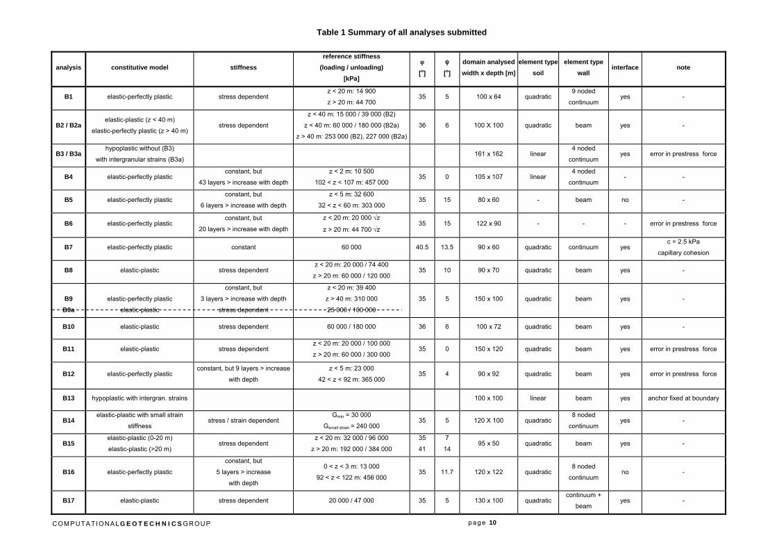
contribute to the differences shown in Figure 4. The corresponding surface displacements depicted in

Figure 5 show differences in settlements behind the wall from approximately 2 to 30 mm.

Fig. 5 Surface settlements after groundwater lowering

5.2.2 Construction stage first excavation step to -4.80 m

Because of possible differences in modelling the groundwater lowering depending on the software

used, it was investigated whether a more clear picture would evolve if a construction stage without the

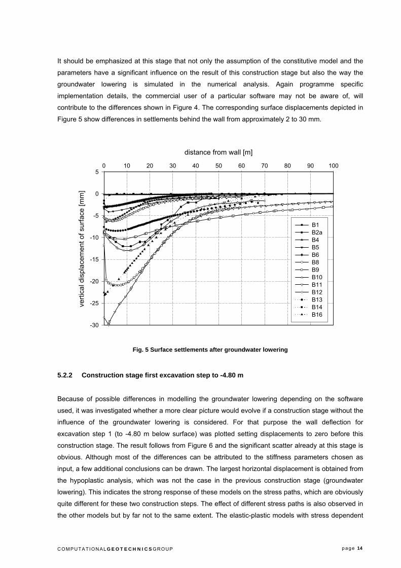
influence of the groundwater lowering is considered. For that purpose the wall deflection for

excavation step 1 (to -4.80 m below surface) was plotted setting displacements to zero before this

construction stage. The result follows from Figure 6 and the significant scatter already at this stage is

obvious. Although most of the differences can be attributed to the stiffness parameters chosen as

input, a few additional conclusions can be drawn. The largest horizontal displacement is obtained from

the hypoplastic analysis, which was not the case in the previous construction stage (groundwater

lowering). This indicates the strong response of these models on the stress paths, which are obviously

quite different for these two construction steps. The effect of different stress paths is also observed in

the other models but by far not to the same extent. The elastic-plastic models with stress dependent


0 10 20 30 40 50 60 70 80 90 100

verti

cal d

ispl

acem

ent o

f sur

face

[mm

]

-30

-25

-20

-15

-10

-5

0

5

B1 B2a B4 B5 B6 B8 B9 B10 B11 B12 B13 B14 B16


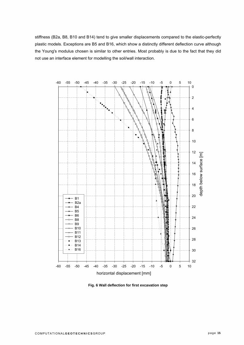
stiffness (B2a, B8, B10 and B14) tend to give smaller displacements compared to the elastic-perfectly

plastic models. Exceptions are B5 and B16, which show a distinctly different deflection curve although

the Young's modulus chosen is similar to other entries. Most probably is due to the fact that they did

not use an interface element for modelling the soil/wall interaction.

Fig. 6 Wall deflection for first excavation step


-60 -55 -50 -45 -40 -35 -30 -25 -20 -15 -10 -5 0 5 10

-60 -55 -50 -45 -40 -35 -30 -25 -20 -15 -10 -5 0 5 10

dept

h be

low

sur

face

[m]

0

2

4

6

8

10

12

14

16

18

20

22

24

26

28

30

32

B1B2aB4B5B6 B8 B9 B10B11B12 B13 B14 B16


5.2.3 Final construction stage

Limited in situ measurements are available for this project and although some simplifications

compared to the actual construction have been introduced for this benchmark exercise in order to

facilitate the calculations, the order of magnitude of displacements can be assumed to be known.

Figure 7 shows the measured wall deflection for the final construction stage together with calculated

values.

Fig. 7 Wall deflection for final excavation step

It should be mentioned that measurements have been taken by inclinometer readings, fixed at the

base of the wall, but unfortunately no geodetic survey of the wall head is available. It is very likely that

the wall base moves horizontally and a parallel shift of the measurement of about 5 to 10 mm is


-80 -70 -60 -50 -40 -30 -20 -10 0 10

-80 -70 -60 -50 -40 -30 -20 -10 0 10

dept

h be

low

sur

face

[m]

0

2

4

6

8

10

12

14

16

18

20

22

24

26

28

30

32

B1B2aB4 B5 B6B8B9B10B11B12 B13 B14B15 B16measurement(corrected)

measurement(corrected)


thought to reflect the in situ behaviour with reasonable accuracy, and therefore the measurement

readings have been shifted by 10 mm in Figure 7. This is confirmed by other measurements under

similar conditions.

The calculated maximum horizontal wall displacement for all results considered varies between

approximately 10 to 65 mm (exception B6). The shape of the deflection curves is also quite different.

Some results indicate the maximum displacement slightly above the final excavation level, others

show the maximum value at the top of the wall. When comparing the results of the calculations with

the measurements it has to be pointed out that the simplification introduced in modelling the

groundwater lowering (one step lowering instead of step-wise lowering according to the excavation

progress) leads to higher horizontal displacements. Further studies revealed that the difference in

calculated horizontal displacements due to the difference in modelling the groundwater lowering is

strongly dependent on the constitutive law employed and ranges in the order of 5 to 15 mm (see also

part II of this report). This may be one of the reasons why B15, which is an elastic-plastic analysis with

stepwise groundwater lowering, is close to the measurement, but it also means that all solutions

predicting less than 30 mm of horizontal displacement are far off reality.

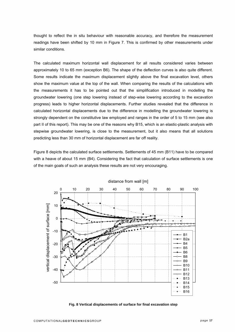
Figure 8 depicts the calculated surface settlements. Settlements of 45 mm (B11) have to be compared

with a heave of about 15 mm (B4). Considering the fact that calculation of surface settlements is one

of the main goals of such an analysis these results are not very encouraging.

Fig. 8 Vertical displacements of surface for final excavation step


0 10 20 30 40 50 60 70 80 90 100

verti

cal d

ispl

acem

ent o

f sur

face

[mm

]

-50

-40

-30

-20

-10

0

10

20

B1 B2a B4 B5 B6 B8 B9 B10 B11 B12 B13 B14 B15 B16


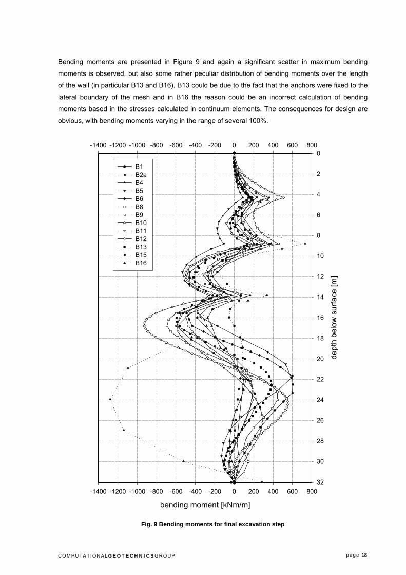
Bending moments are presented in Figure 9 and again a significant scatter in maximum bending

moments is observed, but also some rather peculiar distribution of bending moments over the length

of the wall (in particular B13 and B16). B13 could be due to the fact that the anchors were fixed to the

lateral boundary of the mesh and in B16 the reason could be an incorrect calculation of bending

moments based in the stresses calculated in continuum elements. The consequences for design are

obvious, with bending moments varying in the range of several 100%.

Fig. 9 Bending moments for final excavation step

bending moment [kNm/m]

-1400 -1200 -1000 -800 -600 -400 -200 0 200 400 600 800

-1400 -1200 -1000 -800 -600 -400 -200 0 200 400 600 800

dept

h be

low

sur

face

[m]

0

2

4

6

8

10

12

14

16

18

20

22

24

26

28

30

32

B1B2a B4B5 B6B8 B9 B10 B11 B12B13 B15B16


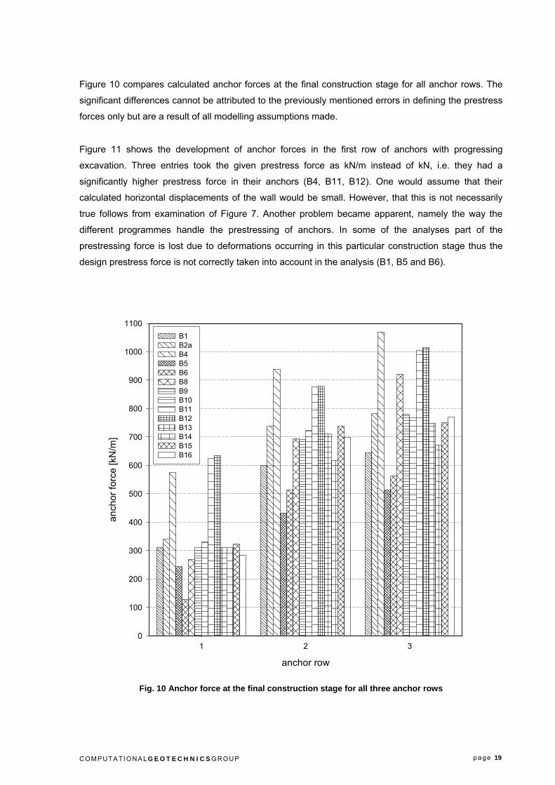
Figure 10 compares calculated anchor forces at the final construction stage for all anchor rows. The

significant differences cannot be attributed to the previously mentioned errors in defining the prestress

forces only but are a result of all modelling assumptions made.

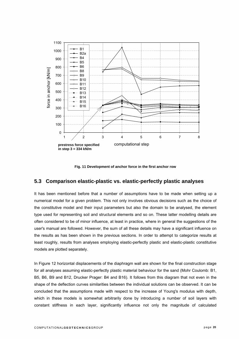
Figure 11 shows the development of anchor forces in the first row of anchors with progressing

excavation. Three entries took the given prestress force as kN/m instead of kN, i.e. they had a

significantly higher prestress force in their anchors (B4, B11, B12). One would assume that their

calculated horizontal displacements of the wall would be small. However, that this is not necessarily

true follows from examination of Figure 7. Another problem became apparent, namely the way the

different programmes handle the prestressing of anchors. In some of the analyses part of the

prestressing force is lost due to deformations occurring in this particular construction stage thus the

design prestress force is not correctly taken into account in the analysis (B1, B5 and B6).

Fig. 10 Anchor force at the final construction stage for all three anchor rows

anchor row

1 2 3

anch

or fo

rce

[kN

/m]

0

100

200

300

400

500

600

700

800

900

1000

1100B1 B2a B4 B5 B6 B8 B9 B10 B11 B12 B13 B14 B15 B16


Fig. 11 Development of anchor force in the first anchor row

5.3 Comparison elastic-plastic vs. elastic-perfectly plastic analyses

It has been mentioned before that a number of assumptions have to be made when setting up a

numerical model for a given problem. This not only involves obvious decisions such as the choice of

the constitutive model and their input parameters but also the domain to be analysed, the element

type used for representing soil and structural elements and so on. These latter modelling details are

often considered to be of minor influence, at least in practice, where in general the suggestions of the

user's manual are followed. However, the sum of all these details may have a significant influence on

the results as has been shown in the previous sections. In order to attempt to categorize results at

least roughly, results from analyses employing elastic-perfectly plastic and elastic-plastic constitutive

models are plotted separately.

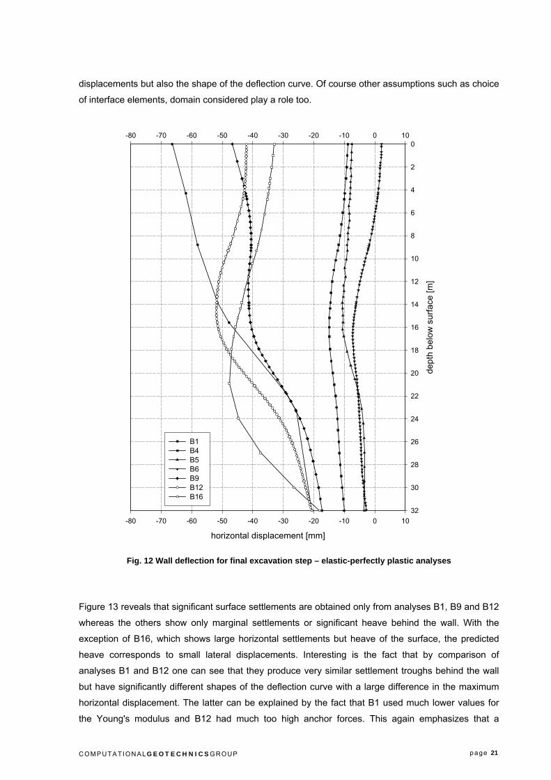
In Figure 12 horizontal displacements of the diaphragm wall are shown for the final construction stage

for all analyses assuming elastic-perfectly plastic material behaviour for the sand (Mohr Coulomb: B1,

B5, B6, B9 and B12, Drucker Prager: B4 and B16). It follows from this diagram that not even in the

shape of the deflection curves similarities between the individual solutions can be observed. It can be

concluded that the assumptions made with respect to the increase of Young's modulus with depth,

which in these models is somewhat arbitrarily done by introducing a number of soil layers with

constant stiffness in each layer, significantly influence not only the magnitude of calculated

computational step

1 2 3 4 5 6 7 8

forc

e in

anc

hor [

kN/m

]

0

100

200

300

400

500

600

700

800

900

1000

1100

B1 B2a B4 B5 B6 B8 B9 B10 B11 B12 B13 B14 B15 B16

prestress force specified in step 3 = 334 kN/m


displacements but also the shape of the deflection curve. Of course other assumptions such as choice

of interface elements, domain considered play a role too.

Fig. 12 Wall deflection for final excavation step – elastic-perfectly plastic analyses

Figure 13 reveals that significant surface settlements are obtained only from analyses B1, B9 and B12

whereas the others show only marginal settlements or significant heave behind the wall. With the

exception of B16, which shows large horizontal settlements but heave of the surface, the predicted

heave corresponds to small lateral displacements. Interesting is the fact that by comparison of

analyses B1 and B12 one can see that they produce very similar settlement troughs behind the wall

but have significantly different shapes of the deflection curve with a large difference in the maximum

horizontal displacement. The latter can be explained by the fact that B1 used much lower values for

the Young's modulus and B12 had much too high anchor forces. This again emphasizes that a


-80 -70 -60 -50 -40 -30 -20 -10 0 10

-80 -70 -60 -50 -40 -30 -20 -10 0 10

dept

h be

low

sur

face

[m]

0

2

4

6

8

10

12

14

16

18

20

22

24

26

28

30

32

B1B4 B5 B6B9B12 B16


number of modelling details have significant influence on displacements, but these effects vary

whether horizontal or vertical displacements are looked at.

Fig. 13 Vertical displacements of surface for final excavation step – elastic-perfectly plastic analyses

Figure 14 summarizes results obtained from elastic-plastic analysis, utilizing the same software and

the same constitutive law. In this case at least the shape of the deflection curves is similar, with

exception of B11, which can be explained by an error in the prestressing force (too high). B10

assumed one homogeneous layer of soil whereas the others introduced 2 layers of soil. Again it is

interesting to see that B2a and B8 produce very similar horizontal displacements although the stiffness

parameters introduced are quite different. However the domain considered in the analysis also differs

(in particular the depth of the mesh) and the combination of these assumptions lead to very similar

results. However, B2a and B8 produce quite different surface settlements. None of the elastic-plastic

solutions leads to the unrealistic heave at the surface behind the wall as observed in some of the

elastic-perfectly plastic analyses (Figure 15).


0 10 20 30 40 50 60 70 80 90 100

verti

cal d

ispl

acem

ent o

f sur

face

[mm

]

-40

-30

-20

-10

0

10

20

B1 B4 B5 B6 B9 B12 B16


Fig. 14 Wall deflection for final excavation step – elastic-plastic analyses

Fig. 15 Vertical displacements of surface for final excavation step – elastic-plastic analyses


-80 -70 -60 -50 -40 -30 -20 -10 0 10

-80 -70 -60 -50 -40 -30 -20 -10 0 10

dept

h be

low

sur

face

[m]

0

2

4

6

8

10

12

14

16

18

20

22

24

26

28

30

32

B2aB8B10B11B15


0 10 20 30 40 50 60 70 80 90 100

verti

cal d

ispl

acem

ent o

f sur

face

[mm

]

-50

-40

-30

-20

-10

0

10

20

B2a B8 B10 B11 B15


6 SUMMARY AND CONCLUSION

Results from a geotechnical benchmark exercise have been presented. A typical problem of a deep

excavation in Berlin sand, formulated by the working group 1.6 of the German Society for

Geotechnics, has been solved by a number of geotechnical engineers from universities and consulting

companies utilizing different finite element codes and constitutive models. Only limited results from

standard laboratory experiments and typical material properties for the sand were provided. Thus it is

claimed that the situation one faces in practice has been addressed where in most cases insufficient

and sometimes not very reliable data, at least as far as stiffness parameters are concerned, are

available and it was part of the game to see how this was handled. Indeed most of the analysts did not

rely on these values and chose stiffness parameters based on their experience resulting in a wide

scatter of input parameters representing the stiffness in the various models. Strength parameters did

not vary significantly.

Thus the comparison of the solutions submitted showed a wide scatter in results and only the most

extreme solutions on the far end of the range could be explained with respect to assumptions of input

parameters made in the analysis. It is clearly evident that matching laboratory experiments with a

particular constitutive model and corresponding material parameters is no guarantee at all to arrive at

a sensible solution for a complex boundary value problem where the soil experiences significantly

different stress paths as compared to the experiments. Some of the results showed obvious errors

such as incorrect prestress forces of anchors but most analyses made reasonable assumptions for

parameters, discretisation and other modelling details.

This benchmark exercise demonstrates the strong need for guidelines and recommendations how to

model typical geotechnical problems in practice. Pitfalls and unrealistic modelling assumptions, the

commercial user may not be aware of, have to be pointed out and procedures have to be developed to

identify these. A strong demand is also put on software developers to thoroughly check their codes

and to clearly document their solution procedures, implementation of constitutive models, structural

and interface elements and other code specific details.

7 REFERENCES

Brinkgreve, R.B.J. & P.A. Vermeer 1998. PLAXIS: Finite Element Code for Soil and Rock Analyses,

Version 7. Balkema.

Carter, J.P, Desai, C.S., Potts, D.M., Schweiger, H.F. & S.W. Sloan 2000. Computing and Computer

Modelling in Geotechnical Engineering. Proc. GeoEng2000, Melbourne, Technomic

Publishing, Lancaster. (Vol. 1: invited papers), 1157-1252.

Duncan, J.M. & C.Y. Chang 1970. Nonlinear analysis of stress and strain in soils. Journal of the Soil

Mechanics and Foundations Division 56, 1629-1653.


Janbu, N. 1963. Soil compressibility as determined by oedometer and triaxial tests. Proceedings

European Conf. On Soil Mechanics and Foundation Engineering, Wiesbaden, Germany, 19-

25.

Meissner, H. 1991. Empfehlungen des Arbeitskreises 1.6 "Numerik in der Geotechnik", Abschnitt 1,

Allgemeine Empfehlungen. Geotechnik, 14, 1-10. (in German)

Meissner, H. 1996. Empfehlungen des Arbeitskreises 1.6 "Numerik in der Geotechnik", Abschnitt 2,

Tunnelbau unter Tage. Geotechnik, 19, 99-108. (in German)

Niemunis, A. & I. Herle 1997. Hypoplastic model for cohesionless soils with elastic strain range.

Mechanics of cohesive-frictional materials, 2, 279-299.

Ohde, J. 1951. Grundbaumechanik (in German), Huette, BD. III, 27. Auflage.

Potts, D.M & L. Zdravkovic (1999). Finite element analysis in geotechnical engineering – Theory.

Thomas Telford

Potts, D.M & L. Zdravkovic (2001). Finite element analysis in geotechnical engineering – Application.

Thomas Telford

Rowe P.W. 1962. The stress-dilatancy relation for static equilibrium of an assembly of particles in

contact. Proc. Roy. Soc. A269, 500-527.

Schweiger, H.F. 1991. Benchmark Problem No. 1: Results. Computers and Geotechnics, 11, 331-341.

Schweiger, H. F. 1998. Results from two geotechnical benchmark problems. Proc. 4th European Conf.

Numerical Methods in Geotechnical Engineering, Cividini, A. (ed.), Springer, 645-654.

Schweiger, H. F. 2000. Ergebnisse des Berechnungsbeispieles Nr. 3 "3-fach verankerte Baugrube".

Tagungsband Workshop "Verformungsprognose für tiefe Baugruben", Stuttgart, 7-67. (in

German)

Schweiger, H.F. 2001. Benchmarking – A new regular section in the bulletin. PLAXIS Bulletin No.11.

PART I: RESULTS OF BENCHMARKING PART II: REFERENCE ...2002...PART I: RESULTS OF BENCHMARKING PART II: REFERENCE SOLUTION AND PARAMETRIC STUDY March 2002 / CGG_IR006_2002 BENCHMARKING

Documents