Part 3 Black Holes Harvey Reall

Welcome message from author
This document is posted to help you gain knowledge. Please leave a comment to let me know what you think about it! Share it to your friends and learn new things together.
Transcript

Part 3 Black Holes
Harvey Reall

Part 3 Black Holes March 3, 2020 ii H.S. Reall

Contents
Preface vii
1 Spherical stars 11.1 Cold stars . . . . . . . . . . . . . . . . . . . . . . . . . . . . . . . . 11.2 Spherical symmetry . . . . . . . . . . . . . . . . . . . . . . . . . . . 21.3 Time-independence . . . . . . . . . . . . . . . . . . . . . . . . . . . 31.4 Static, spherically symmetric, spacetimes . . . . . . . . . . . . . . . 41.5 Tolman-Oppenheimer-Volkoff equations . . . . . . . . . . . . . . . . 51.6 Outside the star: the Schwarzschild solution . . . . . . . . . . . . . 61.7 The interior solution . . . . . . . . . . . . . . . . . . . . . . . . . . 71.8 Maximum mass of a cold star . . . . . . . . . . . . . . . . . . . . . 8
2 The Schwarzschild black hole 112.1 Birkhoff’s theorem . . . . . . . . . . . . . . . . . . . . . . . . . . . 112.2 Gravitational redshift . . . . . . . . . . . . . . . . . . . . . . . . . . 122.3 Geodesics of the Schwarzschild solution . . . . . . . . . . . . . . . . 132.4 Eddington-Finkelstein coordinates . . . . . . . . . . . . . . . . . . . 142.5 Finkelstein diagram . . . . . . . . . . . . . . . . . . . . . . . . . . . 172.6 Gravitational collapse . . . . . . . . . . . . . . . . . . . . . . . . . . 182.7 Black hole region . . . . . . . . . . . . . . . . . . . . . . . . . . . . 192.8 Detecting black holes . . . . . . . . . . . . . . . . . . . . . . . . . . 212.9 White holes . . . . . . . . . . . . . . . . . . . . . . . . . . . . . . . 252.10 The Kruskal extension . . . . . . . . . . . . . . . . . . . . . . . . . 262.11 Einstein-Rosen bridge . . . . . . . . . . . . . . . . . . . . . . . . . . 292.12 Extendibility . . . . . . . . . . . . . . . . . . . . . . . . . . . . . . 302.13 Singularities . . . . . . . . . . . . . . . . . . . . . . . . . . . . . . . 30
3 The initial value problem 333.1 Predictability . . . . . . . . . . . . . . . . . . . . . . . . . . . . . . 333.2 Extrinsic curvature . . . . . . . . . . . . . . . . . . . . . . . . . . . 353.3 The Gauss-Codacci equations . . . . . . . . . . . . . . . . . . . . . 38
iii

CONTENTS
3.4 The constraint equations . . . . . . . . . . . . . . . . . . . . . . . . 40
3.5 The initial value problem in GR . . . . . . . . . . . . . . . . . . . . 41
3.6 Asymptotically flat initial data . . . . . . . . . . . . . . . . . . . . 43
3.7 Strong cosmic censorship . . . . . . . . . . . . . . . . . . . . . . . . 44
4 The singularity theorem 47
4.1 Null hypersurfaces . . . . . . . . . . . . . . . . . . . . . . . . . . . 47
4.2 Geodesic deviation . . . . . . . . . . . . . . . . . . . . . . . . . . . 49
4.3 Geodesic congruences . . . . . . . . . . . . . . . . . . . . . . . . . . 50
4.4 Null geodesic congruences . . . . . . . . . . . . . . . . . . . . . . . 51
4.5 Expansion, rotation and shear . . . . . . . . . . . . . . . . . . . . . 52
4.6 Expansion and shear of a null hypersurface . . . . . . . . . . . . . . 53
4.7 Trapped surfaces . . . . . . . . . . . . . . . . . . . . . . . . . . . . 55
4.8 Raychaudhuri’s equation . . . . . . . . . . . . . . . . . . . . . . . . 57
4.9 Energy conditions . . . . . . . . . . . . . . . . . . . . . . . . . . . . 57
4.10 Conjugate points . . . . . . . . . . . . . . . . . . . . . . . . . . . . 59
4.11 Causal structure . . . . . . . . . . . . . . . . . . . . . . . . . . . . . 61
4.12 Penrose singularity theorem . . . . . . . . . . . . . . . . . . . . . . 64
5 Asymptotic flatness 67
5.1 Conformal compactification . . . . . . . . . . . . . . . . . . . . . . 67
5.2 Asymptotic flatness . . . . . . . . . . . . . . . . . . . . . . . . . . . 73
5.3 Definition of a black hole . . . . . . . . . . . . . . . . . . . . . . . . 78
5.4 Weak cosmic censorship . . . . . . . . . . . . . . . . . . . . . . . . 80
5.5 Apparent horizon . . . . . . . . . . . . . . . . . . . . . . . . . . . . 83
6 Charged black holes 85
6.1 The Reissner-Nordstrom solution . . . . . . . . . . . . . . . . . . . 85
6.2 Eddington-Finkelstein coordinates . . . . . . . . . . . . . . . . . . . 86
6.3 Kruskal-like coordinates . . . . . . . . . . . . . . . . . . . . . . . . 87
6.4 Cauchy horizons . . . . . . . . . . . . . . . . . . . . . . . . . . . . . 90
6.5 Extreme RN . . . . . . . . . . . . . . . . . . . . . . . . . . . . . . . 92
6.6 Majumdar-Papapetrou solutions . . . . . . . . . . . . . . . . . . . . 94
7 Rotating black holes 97
7.1 Uniqueness theorems . . . . . . . . . . . . . . . . . . . . . . . . . . 97
7.2 The Kerr-Newman solution . . . . . . . . . . . . . . . . . . . . . . 99
7.3 The Kerr solution . . . . . . . . . . . . . . . . . . . . . . . . . . . . 100
7.4 Maximal analytic extension . . . . . . . . . . . . . . . . . . . . . . 101
7.5 The ergosphere and Penrose process . . . . . . . . . . . . . . . . . . 103
Part 3 Black Holes March 3, 2020 iv H.S. Reall

CONTENTS
8 Mass, charge and angular momentum 1078.1 Charges in curved spacetime . . . . . . . . . . . . . . . . . . . . . . 1078.2 Komar integrals . . . . . . . . . . . . . . . . . . . . . . . . . . . . . 1098.3 Hamiltonian formulation of GR . . . . . . . . . . . . . . . . . . . . 1118.4 ADM energy . . . . . . . . . . . . . . . . . . . . . . . . . . . . . . . 115
9 Black hole mechanics 1179.1 Killling horizons and surface gravity . . . . . . . . . . . . . . . . . . 1179.2 Interpretation of surface gravity . . . . . . . . . . . . . . . . . . . . 1199.3 Zeroth law of black holes mechanics . . . . . . . . . . . . . . . . . . 1209.4 First law of black hole mechanics . . . . . . . . . . . . . . . . . . . 1219.5 Second law of black hole mechanics . . . . . . . . . . . . . . . . . . 125
10 Quantum field theory in curved spacetime 12910.1 Introduction . . . . . . . . . . . . . . . . . . . . . . . . . . . . . . . 12910.2 Quantization of the free scalar field . . . . . . . . . . . . . . . . . . 13010.3 Bogoliubov transformations . . . . . . . . . . . . . . . . . . . . . . 13310.4 Particle production in a non-stationary spacetime . . . . . . . . . . 13410.5 Rindler spacetime . . . . . . . . . . . . . . . . . . . . . . . . . . . . 13510.6 Wave equation in Schwarzschild spacetime . . . . . . . . . . . . . . 14110.7 Hawking radiation . . . . . . . . . . . . . . . . . . . . . . . . . . . 14310.8 Black hole thermodynamics . . . . . . . . . . . . . . . . . . . . . . 15210.9 Black hole evaporation . . . . . . . . . . . . . . . . . . . . . . . . . 153
Part 3 Black Holes March 3, 2020 v H.S. Reall

CONTENTS
Part 3 Black Holes March 3, 2020 vi H.S. Reall

Preface
These are lecture notes for the course on Black Holes in Part III of the CambridgeMathematical Tripos.
Acknowledgment
I am grateful to Andrius Stikonas and Josh Kirklin for producing most of thefigures.
Conventions
We will use units such that the speed of light is c = 1 and Newton’s constant isG = 1. This implies that length, time and mass have the same units.
The metric signature is (−+ ++)
The cosmological constant is so small that is is important only on the largestlength scales, i.e., in cosmology. We will assume Λ = 0 in this course.
We will use abstract index notation. Greek indices µ, ν, . . . refer to tensorcomponents with respect to some basis. Such indices take values from 0 to 3. Anequation written with such indices is valid only in a particular basis. Spacetimecoordinates are denoted xµ. Abstract indices are Latin indices a, b, c . . .. Theseare used to denote tensor equations, i.e., equations valid in any basis. Any objectcarrying abstract indices must be a tensor of the type indicates by its indices e.g.Xa
b is a tensor of type (1, 1). Any equation written with abstract indices can bewritten out in a basis by replacing Latin indices with Greek ones (a → µ, b → νetc). Conversely, if an equation written with Greek indices is valid in any basisthen Greek indices can be replaced with Latin ones.
For example: Γµνρ = 12gµσ (gσν,ρ + gσρ,ν − gνρ,σ) is valid only in a coordinate
basis. Hence we cannot write it using abstract indices. But R = gabRab is a tensorequation so we can use abstract indices.
Riemann tensor: R(X, Y )Z = ∇X∇YZ −∇Y∇XZ −∇[X,Y ]Z.
vii

CHAPTER 0. PREFACE
Bibliography
1. N.D. Birrell and P.C.W. Davies, Quantum fields in curved space, CambridgeUniversity Press, 1982.
2. Spacetime and Geometry, S.M. Carroll, Addison Wesley, 2004.
3. V.P. Frolov and I.D. Novikov, Black holes physics, Kluwer, 1998.
4. S.W. Hawking and G.F.R. Ellis, The large scale structure of space-time,Cambridge University Press, 1973.
5. R.M. Wald, General relativity, University of Chicago Press, 1984.
6. R.M. Wald, Quantum field theory in curved spacetime and black hole ther-modynamics, University of Chicago Press, 1994.
Most of this course concerns classical aspects of black hole physics. The booksthat I found most useful in preparing this part of the course are Wald’s GR book,and Hawking and Ellis. The final chapter of this course concerns quantum fieldtheory in curved spacetime. Here I mainly used Birrell and Davies, and Wald’ssecond book. The latter also contains a nice discussion of the laws of black holemechanics.
Part 3 Black Holes March 3, 2020 viii H.S. Reall

Chapter 1
Spherical stars
1.1 Cold stars
To understand the astrophysical significance of black holes we must discuss stars.In particular, how do stars end their lives?
A normal star like our Sun is supported against contracting under its owngravity by pressure generated by nuclear reactions in its core. However, eventuallythe star will use up its nuclear “fuel”. If the gravitational self-attraction is to bebalanced then some new source of pressure is required. If this balance is to lastforever then this new source of pressure must be non-thermal because the star willeventually cool.
A non-thermal source of pressure arises quantum mechanically from the Pauliprinciple, which makes a gas of cold fermions resist compression (this is calleddegeneracy pressure). A white dwarf is a star in which gravity is balanced byelectron degeneracy pressure. The Sun will end its life as a white dwarf. Whitedwarfs are very dense compared to normal stars e.g. a white dwarf with the samemass as the Sun would have a radius around a hundredth of that of the Sun. UsingNewtonian gravity one can show that a white dwarf cannot have a mass greaterthan the Chandrasekhar limit 1.4M where M is the mass of the Sun. A starmore massive than this cannot end its life as a white dwarf (unless it somehowsheds some of its mass).
Once the density of matter approaches nuclear density, the degeneracy pressureof neutrons becomes important (at such high density, inverse beta decay convertsprotons into neutrons). A neutron star is supported by the degeneracy pressure ofneutrons. These stars are tiny: a solar mass neutron star would have a radius ofaround 10km (the radius of the Sun is 7×10⁵km). Recall that validity of Newtoniangravity requires |Φ| 1 where Φ is the Newtonian gravitational potential. At thesurface of a such a neutron star one has |Φ| ∼ 0.1 and so a Newtonian description
1

CHAPTER 1. SPHERICAL STARS
is inadequate: one has to use GR.In this chapter we will see that GR predicts that there is a maximum mass
for neutron stars. Remarkably, this is independent of the (unknown) propertiesof matter at extremely high density and so it holds for any cold star. As wewill explain, detailed calculations reveal the maximum mass to be around 3M.Hence a hot star more massive than this cannot end its life as a cold star (unlessit sheds some mass e.g. in a supernova). Instead the star will undergo completegravitational collapse to form a black hole.
In the next few sections we will show that GR predicts a maximum mass fora cold star. We will make the simplifying assumption that the star is sphericallysymmetric. As we will see, the Schwarzschild solution is the unique sphericallysymmetric vacuum solution and hence describes the gravitational field outsideany spherically symmetric star. The interior of the star can be modelled using aperfect fluid and so spacetime inside the star is determined by solving the Einsteinequation with a perfect fluid source and matching onto the Schwarzschild solutionoutside the star.
1.2 Spherical symmetry
We need to define what we mean by a spacetime being spherically symmetric. Youare familiar with the idea that a round sphere is invariant under rotations, whichform the group SO(3). In more mathematical language, this can be phrased asfollows. The set of all isometries of a manifold with metric forms a group. Considerthe unit round metric on S2:
dΩ2 = dθ2 + sin2 θ dφ2. (1.1)
The isometry group of this metric is SO(3) (actually O(3) if we include reflections).Any 1-dimensional subgroup of SO(3) gives a 1-parameter group of isometries, andhence a Killing vector field. A spacetime is spherically symmetric if it possessesthe same symmetries as a round S2:
Definition. A spacetime is spherically symmetric if its isometry group containsan SO(3) subgroup whose orbits are 2-spheres. (The orbit of a point p under agroup of diffeomorphisms is the set of points that one obtains by acting on p withall of the diffeomorphisms.)
The statement about the orbits is important: there are examples of spacetimeswith SO(3) isometry group in which the orbits of SO(3) are 3-dimensional (e.g.Taub-NUT space: see Hawking and Ellis).
Definition. In a spherically symmetric spacetime, the area-radius function r :M → R is defined by r(p) =
√A(p)/4π where A(p) is the area of the S2 orbit
Part 3 Black Holes March 3, 2020 2 H.S. Reall

1.3. TIME-INDEPENDENCE
through p. (In other words, the S2 passing through p has induced metric r(p)2dΩ2.)
1.3 Time-independence
Definition. A spacetime is stationary if it admits a Killing vector field ka whichis everywhere timelike: gabk
akb < 0.
We can choose coordinates as follows. Pick a hypersurface Σ nowhere tangentto ka and introduce coordinates xi on Σ. Assign coordinates (t, xi) to the pointparameter distance t along the integral curve through the point on Σ with coor-dinates xi. This gives a coordinates chart such that ka = (∂/∂t)a. Since ka is aKilling vector field, the metric is independent of t and hence takes the form
ds2 = g00(xk)dt2 + 2g0i(xk)dtdxi + gij(x
k)dxidxj (1.2)
where g00 < 0. Conversely, given a metric of this form, ∂/∂t is obviously a timelikeKilling vector field and so the metric is stationary.
Next we need to introduce the notion of hypersurface-orthogonality. Let Σ be ahypersurface in M specified by f(x) = 0 where f : M → R is smooth with df 6= 0on Σ. Then the 1-form df is normal to Σ. (Proof: let ta be any vector tangent toΣ then df(t) = t(f) = tµ∂µf = 0 because f is constant on Σ.) Any other 1-formn normal to Σ can be written as n = gdf + fn′ where g is a smooth function withg 6= 0 on Σ and n′ is a smooth 1-form. Hence we have dn = dg∧df +df ∧n′+fdn′
so (dn)|Σ = (dg − n′) ∧ df . So if n is normal to Σ then
(n ∧ dn)|Σ = 0 (1.3)
Conversely:
Theorem (Frobenius). If n is a non-zero 1-form such that n∧ dn = 0 everywherethen there exist functions f, g such that n = gdf so n is normal to surfaces ofconstant f i.e. n is hypersurface-orthogonal.
Definition. A spacetime is static if it admits a hypersurface-orthogonal timelikeKilling vector field. (So static implies stationary.)
For a static spacetime, we know that ka is hypersurface-orthogonal so when defin-ing coordinates (t, xi) we can choose Σ to be orthogonal to ka. But Σ is thesurface t = 0, with normal dt. It follows that, at t = 0, kµ ∝ (1, 0, 0, 0) in ourchart, i.e., ki = 0. However ki = g0i(x
k) so we must have g0i(xk) = 0. So in
adapted coordinates a static metric takes the form
ds2 = g00(xk)dt2 + gij(xk)dxidxj (1.4)
Part 3 Black Holes March 3, 2020 3 H.S. Reall

CHAPTER 1. SPHERICAL STARS
where g00 < 0. Note that this metric has a discrete time-reversal isometry:(t, xi) → (−t, xi). So static means ”time-independent and invariant under timereversal”. For example, the metric of a rotating star can be stationary but notstatic because time-reversal changes the sense of rotation.
1.4 Static, spherically symmetric, spacetimes
We’re interested in determining the gravitational field of a time-independent spher-ical object so we assume our spacetime to be stationary and spherically symmetric.By this we mean that the isometry group is R × SO(3) where the the R factorcorresponds to “time translations” (i.e., the associated Killing vector field is time-like) and the orbits of SO(3) are 2-spheres as above. It can be shown that anysuch spacetime must actually be static. (The gravitational field of a rotating starcan be stationary but the rotation defines a preferred axis and so the spacetimewould not be spherically symmetric.) So let’s consider a spacetime that is bothstatic and spherically symmetric.
Staticity means that we have a timelike Killing vector field ka and we can foliateour spacetime with surfaces Σt orthogonal to ka. One can argue that the orbit ofSO(3) through p ∈ Σt lies within Σt. We can define spherical polar coordinates onΣ0 as follows. Pick a S2 symmetry orbit in Σ0 and define spherical polars (θ, φ) onit. Extend the definition of (θ, φ) to the rest of Σ0 by defining them to be constantalong (spacelike) geodesics normal to this S2 within Σ0. Now we use (r, θ, φ) ascoordinates on Σ0 where r is the area-radius function defined above. The metricon Σ0 must take the form
ds2 = e2Ψ(r)dr2 + r2dΩ2 (1.5)
drdθ and drdφ terms cannot appear because they would break spherical symmetry.Note that r is not “the distance from the origin”. Finally, we define coordinates(t, r, θ, φ) with t the parameter distance from Σ0 along the integral curves of ka.The metric must take the form
ds2 = −e2Φ(r)dt2 + e2Ψ(r)dr2 + r2dΩ2 (1.6)
The matter inside a star can be described by a perfect fluid, with energy momentumtensor
Tab = (ρ+ p)uaub + pgab (1.7)
where ua is the 4-velocity of the fluid (a unit timelike vector: gabuaub = −1), and
ρ,p are the energy density and pressure measured in the fluid’s local rest frame(i.e. by an observer with 4-velocity ua).
Part 3 Black Holes March 3, 2020 4 H.S. Reall

1.5. TOLMAN-OPPENHEIMER-VOLKOFF EQUATIONS
Since we’re interested in a time-independent and spherically symmetric situa-tion we assume that the fluid is at rest, so ua is in the time direction:
ua = e−Φ
(∂
∂t
)a(1.8)
Our assumptions of staticity and spherical symmetry implies that ρ and p dependonly on r. Let R denote the (area-)radius of the star. Then ρ and p vanish forr > R.
1.5 Tolman-Oppenheimer-Volkoff equations
Recall that the fluid’s equations of motion are determined by energy-momentumtensor conservation. But the latter follows from the Einstein equation and thecontracted Bianchi identity. Hence we can obtain the equations of motion fromjust the Einstein equation. Now the Einstein tensor inherits the symmetries of themetric and so there are only three non-trivial components of the Einstein equation.These are the tt, rr and θθ components (spherical symmetry implies that the φφcomponent is proportional to the θθ component). You are asked to calculate theseon examples sheet 1.
Define m(r) by
e2Ψ(r) =
(1− 2m(r)
r
)−1
(1.9)
and note that the LHS is positive so m(r) < r/2. The tt component of the Einsteinequation gives
dm
dr= 4πr2ρ (1.10)
The rr component of the Einstein equation gives
dΦ
dr=m+ 4πr3p
r(r − 2m)(1.11)
The final non-trivial component of the Einstein equation is the θθ componentThis gives a third equation of motion. But this is more easily derived from ther-component of energy-momentum conservation ∇µT
µν = 0, i.e., from the fluidequations of motion. This gives
dp
dr= −(p+ ρ)
(m+ 4πr3p)
r(r − 2m)(1.12)
We have 3 equations but 4 unknowns (m,Φ, ρ, p) so we need one more equation.We are interested in a cold star, i.e., one with vanishing temperature T . Thermo-dynamics tells us that T , p and ρ are not independent: they are related by the
Part 3 Black Holes March 3, 2020 5 H.S. Reall

CHAPTER 1. SPHERICAL STARS
fluid’s equation of state e.g. T = T (ρ, p). Hence the condition T = 0 implies arelation between p and ρ, i.e, a barotropic equation of state p = p(ρ). So, for acold star, p is not an independent variable so we have 3 equations for 3 unknowns.These are called the Tolman-Oppenheimer-Volkoff equations.
We assume that ρ > 0 and p > 0, i.e., the energy density and pressure ofmatter are positive. We also assume that p is an increasing function of ρ. If thiswere not the case then the fluid would be unstable: a fluctuation in some regionthat led to an increase in ρ would decrease p, causing the fluid to move into thisregion and hence further increase in ρ, i.e., the fluctuation would grow.
1.6 Outside the star: the Schwarzschild solution
Consider first the spacetime outside the star: r > R. We then have ρ = p = 0.For r > R (1.10) gives m(r) = M , constant. Integrating (1.11) gives
Φ =1
2log (1− 2M/r) + Φ0 (1.13)
for some constant Φ0. We then have gtt → −e2Φ0 as r → ∞. The constant Φ0
can be eliminated by defining a new time coordinate t′ = eΦ0t. So without loss ofgenerality we can set Φ0 = 0 and we have arrived at the Schwarzschild solution
ds2 = −(
1− 2M
r
)dt2 +
(1− 2M
r
)−1
dr2 + r2dΩ2 (1.14)
The constant M is the mass of the star. One way to see this is to note thatfor large r, the Schwarzschild solution reduces to the solution of linearized theorydescribing the gravitational field far from a body of mass M (a change of radialcoordinate is required to see this). We will give a precise definition of mass laterin this course.
The components of the above metric are singular at the Schwarzschild radiusr = 2M , where gtt vanishes and grr diverges. A solution describing a static spher-ically symmetric star can exist only if r = 2M corresponds to a radius inside thestar, where the Schwarzschild solution does not apply. Hence a static, sphericallysymmetric star must have a radius greater than its Schwarzschild radius:
R > 2M (1.15)
Normal stars have R 2M e.g. for the Sun, 2M ≈ 3km whereas R ≈ 7× 10⁵km.
Part 3 Black Holes March 3, 2020 6 H.S. Reall

1.7. THE INTERIOR SOLUTION
1.7 The interior solution
Integrating (1.10) gives
m(r) = 4π
∫ r
0
ρ(r′)r′2dr′ +m? (1.16)
where m? is a constant.Now Σt should be smooth at r = 0 (the centre of the star). Recall that any
smooth Riemannian manifold is locally flat, i.e., measurements in a sufficientlysmall region will be the same as in Euclidean space. In Euclidean space, a sphereof area-radius r also has proper radius r, i.e., all points on the sphere lie properdistance r from the centre. Hence the same must be true for a small sphere onΣt. The proper radius of a sphere of area-radius r is
∫ r0eΨ(r′)dr′ ≈ eΨ(0)r for small
r. Hence we need eΨ(0) = 1 for the metric to be smooth at r = 0. This impliesm(0) = 0 and so m? = 0.
Now at r = R, our interior solution must match onto the exterior Schwarzschildsolution. For r > R we have m(r) = M so continuity of m(r) determines M :
M = 4π
∫ R
0
ρ(r)r2dr (1.17)
This is formally the same as the equation relating total mass to density in Newto-nian theory. But there is an important difference: in the Euclidean space of New-tonian theory, the volume element on a surface of constant t is r2 sin θdr∧ dθ∧ dφand so the RHS above gives the total energy of matter. However, in GR, thevolume element on Σt is eΨr2 sin θdr ∧ dθ ∧ dφ so the total energy of the matter is
E = 4π
∫ R
0
ρeΨr2dr (1.18)
and since eΨ > 1 (as m > 0) we have E > M : the energy of the matter in thestar is greater than the total energy M of the star. The difference E −M can beinterpreted as the gravitational binding energy of the star.
In GR there is a lower limit on the size of stars that has no Newtonian analogue.To see this, note that the definition (1.9) implies m(r)/r < 1/2 for all r. Evaluatingat r = R recovers the result R > 2M discussed above. (To see that this has noNewtonian analogue, we can reinsert factors of G and c to write it as GM/(c2R) <1/2. Taking the Newtonian limit c→∞ the equation becomes trivial.)
This lower bound can be improved. Note that (1.12) implies dp/dr ≤ 0 andhence dρ/dr ≤ 0. Using this it can be shown (examples sheet 1) that
m(r)
r<
2
9
[1− 6πr2p(r) + (1 + 6πr2p(r))1/2
](1.19)
Part 3 Black Holes March 3, 2020 7 H.S. Reall

CHAPTER 1. SPHERICAL STARS
Evaluating at r = R we have p = 0 and hence obtain the Buchdahl inequality
R >9
4M (1.20)
The derivation of this inequality assumes only ρ ≥ 0 and dρ/dr ≤ 0 and nothingabout the equation of state, so it also applies to hot stars satisfying these assump-tions. This inequality is sharp: on examples sheet 1 it is shown that stars withconstant density ρ can get arbitrarily close to saturating it (the pressure at thecentre diverges in the limit in which the inequality becomes an equality).
The TOV equations can be solved by numerical integration as follows. Regard(1.10) and (1.12) as a pair of coupled first order ordinary differential equations form(r) and ρ(r) (recall that p = p(ρ) and dp/dρ > 0). These can be solved, at leastnumerically on a computer, given initial conditions for m(r) and ρ(r) at r = 0.We have just seen that m(0) = 0. Hence just need to specify the value ρc = ρ(0)for the density at the centre of the star.
Given a value for ρc we can solve (1.10) and (1.12). The latter equation showsthat p (and hence ρ) decreases as r increases. Since the pressure vanishes at thesurface of the star, the radius R is determined by the condition p(R) = 0. Thisdetermines R as a function of ρc. Equation (1.17) then determines M as a functionof ρc. Finally we determine Φ(r) inside the star by integrating (1.11) inwards fromr = R with initial condition Φ(R) = (1/2) log(1 − 2M/R) (from (1.13)). Hence,for a given equation of state, static, spherically symmetric, cold stars form a 1-parameter family of solutions, labelled by ρc.
1.8 Maximum mass of a cold star
When one follows the above procedure then one finds that, as ρc increases, Mincreases to a maximum value but then decreases for larger ρc as shown in Fig.1.1.
The maximum mass will depend on the details of the equation of state of coldmatter. For example, taking an equation of state corresponding to white dwarfmatter reproduces the Chandrasekhar bound (as mentioned above, one does notneed GR for this, it can be obtained using Newtonian gravity). Experimentally weknow this equation of state up to some density ρ0 (around nuclear density) but wedon’t know its form for ρ > ρ0. One might expect that by an appropriate choiceof the equation of state for ρ > ρ0 one could arrange for the maximum mass tobe very large, say 100M. This is not the case. Remarkably, GR predicts thatthere is an upper bound on the mass of a cold, spherically symmetric star, whichis independent of the form of the equation of state at high density. This upperbound is around 5M.
Part 3 Black Holes March 3, 2020 8 H.S. Reall

1.8. MAXIMUM MASS OF A COLD STAR
M
ρ0
Figure 1.1: Plot of M against ρc for typical equation of state.
Recall that ρ is a decreasing function of r. Define the core of the star as theregion in which ρ > ρ0 where we don’t know the equation of state and the envelopeas the region ρ < ρ0 where we do know the equation of state. Let r0 be the radius ofthe core, i.e., the core is the region r < r0 and the envelope the region r0 < r < R.The mass of the core is defined as m0 = m(r0). Equation (1.16) gives
m0 ≥4
3πr3
0ρ0 (1.21)
We would have the same result in Newtonian gravity. In GR we have the extraconstraint (1.19). Evaluating this at r = r0 gives
m0
r0
<2
9
[1− 6πr2
0p0 + (1 + 6πr20p0)1/2
](1.22)
where p0 = p(r0) is determined from ρ0 using the equation of state. Note that theRHS is a decreasing function of p0 so we obtain a simpler (but weaker) inequalityby evaluating the RHS at p0 = 0:
m0 <4
9r0 (1.23)
i.e., the core satisfies the Buchdahl inequality. The two inequalities (1.21) and(1.23) define a finite region of the m0 − r0 plane: The upper bound on the massof the core is
m0 <
√16
243πρ0
(1.24)
Part 3 Black Holes March 3, 2020 9 H.S. Reall

CHAPTER 1. SPHERICAL STARS
m0
r0
Figure 1.2: Allowed region of m0 − r0 plane
Hence although we don’t know the equation of state inside the core, GR predictsthat its mass cannot be indefinitely large. Experimentally, we don’t know theequation of state of cold matter at densities much higher than the density ofatomic nuclei so we take ρ0 = 5× 10¹⁴ g/cm3, the density of nuclear matter. Thisgives an upper bound on the core mass m0 < 5M.
Now, given a core with massm0 and radius r0, the envelope region is determineduniquely by solving numerically (1.10) and (1.12) with initial conditions m = m0
and ρ = ρ0 at r = r0, using the known equation of state at density ρ < ρ0. Thisshow that the total mass M of the star is a function of the core parameters m0
and r0. By investigating (numerically) the behaviour of this function as m0 andr0 range over the allowed region of the above Figure, it is found that the M ismaximised at the maximum of m0 (actually one uses the stricter inequality (1.22)instead of (1.23) to define the allowed region). At this maximum, the envelopecontributes less than 1% of the total mass so the maximum value of M is almostthe same as the maximum value of m0, i.e., 5M.
It should be emphasized that this is an upper bound that applies for anyphysically reasonable equation of state for ρ > ρ0. But any particular equationof state will have its own upper bound, which will be less than the above bound.Indeed, one can improve the above bound by adding further criteria to what onemeans by ”physically reasonable”. For example, the speed of sound in the fluid is(dp/dρ)1/2. It is natural to demand that this should not exceed the speed of light,i.e. one could add the extra condition dp/dρ ≤ 1. This has the effect of reducingthe upper bound to about 3M.
Part 3 Black Holes March 3, 2020 10 H.S. Reall

Chapter 2
The Schwarzschild black hole
We have seen that GR predicts that a cold star cannot have a mass more than afew times M. A very massive hot star cannot end its life as a cold star unless itsomehow sheds some of its mass. Instead it will undergo complete gravitationalcollapse to form a black hole. The simplest black hole solution is described bythe Schwarzschild geometry. So far, we have used the Schwarzschild metric todescribe the spacetime outside a spherical star. In this chapter we will investigatethe geometry of spacetime under the assumption that the Schwarzschild solutionis valid everywhere, i.e., no matter is present.
2.1 Birkhoff’s theorem
In Schwarzschild coordinates (t, r, θ, φ), the Schwarzschild solution is
ds2 = −(
1− 2M
r
)dt2 +
(1− 2M
r
)−1
dr2 + r2dΩ2 (2.1)
This is actually a 1-parameter family of solutions. The parameter M take eithersign but, as mentioned above, it has the interpretation of a mass so we will assumeM > 0 here. The case M < 0 will be discussed later.
Previously we assumed that we were dealing with r > 2M . But the abovemetric is also a solution of the vacuum Einstein equation for 0 < r < 2M . We willsee below how these are related. r = 2M is called the Schwarzschild radius.
We derived the Schwarzschild solution under the assumptions of staticity andspherical symmetry. It turns out that the former is not required:
Theorem (Birkhoff). Any spherically symmetric solution of the vacuum Ein-stein equation is isometric to the Schwarzschild solution.
Proof. See Hawking and Ellis.
11

CHAPTER 2. THE SCHWARZSCHILD BLACK HOLE
This theorem assumes only spherical symmetry but the Schwarzschild solutionhas an additional isometry: ∂/∂t is a hypersurface-orthogonal Killing vector field.It is timelike for r > 2M so the r > 2M Schwarzschild solution is static.
Birkhoff’s theorem implies that the spacetime outside any spherical body isdescribed by the time-independent (exterior) Schwarzschild solution. This is trueeven if the body itself is time-dependent. For example, consider a spherical starthat ”uses up its nuclear fuel” and collapses to form a white dwarf or neutronstar. The spacetime outside the star will be described by the static Schwarzschildsolution even during the collapse.
2.2 Gravitational redshift
Consider two observers A and B who remain at fixed (r, θ, φ) in the Schwarzschildgeometry. Let A have r = rA and B have r = rB where rB > rA. Now assumethat A sends two photons to B separated by a coordinate time ∆t as measuredby A. Since ∂/∂t is an isometry, the path of the second photon is the same as thepath of the first one, just translated in time through an interval ∆t.
Exercise. Show that the proper time between the photons emitted by A, asmeasured by A is ∆τA =
√1− 2M/rA∆t.
Similarly the proper time interval between the photons received by B, as mea-sured by B is ∆τB =
√1− 2M/rB∆t. Eliminating ∆t gives
∆τB∆τA
=
√1− 2M/rB1− 2M/rA
> 1 (2.2)
Now imagine that we are considering light waves propagating from A to B. Apply-ing the above argument to two successive wavecrests shows that the above formularelates the period ∆τA of the waves emitted by A to the period ∆τB of the wavesreceived by B. For light, the period is the same as the wavelength (since c = 1):∆τ = λ. Hence λB > λA: the light undergoes a redshift as it climbs out of thegravitational field.
If B is at large radius, i.e., rB 2M , then we have
1 + z ≡ λBλA
=
√1
1− 2M/rA(2.3)
Note that this diverges as rA → 2M . We showed above that a spherical star musthave radius R > 9M/4 so (taking rA = R) it follows that the maximum possibleredshift of light emitted from the surface of a spherical star is z = 2.
Part 3 Black Holes March 3, 2020 12 H.S. Reall

2.3. GEODESICS OF THE SCHWARZSCHILD SOLUTION
2.3 Geodesics of the Schwarzschild solution
Let xµ(τ) be an affinely parameterized geodesic with tangent vector uµ = dxµ/dτ .Since k = ∂/∂t and m = ∂/∂φ are Killing vector fields we have the conservedquantities
E = −k · u =
(1− 2M
r
)dt
dτ(2.4)
and
h = m · u = r2 sin2 θdφ
dτ(2.5)
For a timelike geodesic, we choose τ to be proper time and then E has the inter-pretation of energy per unit rest mass and h is the angular momentum per unitrest mass. (To see this, evaluate the expressions for E and h at large r wherethe metric is almost flat so one can use results from special relativity.) For a nullgeodesic, the freedom to rescale the affine parameter implies that E and h do nothave direct physical significance. However, the ratio h/E is invariant under thisrescaling. For a null geodesic which propagates to large r (where the metric isalmost flat and the geodesic is a straight line), b = |h/E| is the impact parameter,i.e., the distance of the null geodesic from ”a line through the origin”, more pre-cisely the distance from a line of constant φ parallel (at large r) to the geodesic.
Exercise. Determine the Euler-Lagrange equation for θ(τ) and eliminate dφ/dτto obtain
r2 d
dτ
(r2 dθ
dτ
)− h2 cos θ
sin3 θ= 0 (2.6)
One can define spherical polar coordinates on S2 in many different ways. It is
convenient to rotate our (θ, φ) coordinates so that our geodesic has θ = π/2 anddθ/dτ = 0 at τ = 0, i.e., the geodesic initially lies in, and is moving tangentiallyto, the ”equatorial plane” θ = π/2. We emphasize: this is just a choice of thecoordinates (θ, φ). Now, whatever r(τ) is (and we don’t know yet), the aboveequation is a second order ODE for θ with initial conditions θ = π/2, dθ/dτ =0. One solution of this initial value problem is θ(τ) = π/2 for all τ . Standarduniqueness results for ODEs guarantee that this is the unique solution. Hence wehave shown that we can always choose our θ, φ coordinates so that the geodesic isconfined to the equatorial plane. We shall assume this henceforth.
Exercise. Choosing τ to be proper time in the case of a timelike geodesic, and ar-clength (proper distance) in the case of a spacelike geodesic implies gµνu
µuν = −σwhere σ = 1, 0,−1 for a timelike, null or spacelike geodesic respectively. Rearrange
Part 3 Black Holes March 3, 2020 13 H.S. Reall

CHAPTER 2. THE SCHWARZSCHILD BLACK HOLE
this equation to obtain
1
2
(dr
dτ
)2
+ V (r) =1
2E2 (2.7)
where
V (r) =1
2
(1− 2M
r
)(σ +
h2
r2
)(2.8)
Hence the radial motion of the geodesic is determined by the same equation as aNewtonian particle of unit mass and energy E2/2 moving in a 1d potential V (r).
2.4 Eddington-Finkelstein coordinates
Consider the Schwarzschild solution with r > 2M . Let’s consider the simplesttype of geodesic: radial null geodesics. ”Radial” means that θ and φ are constantalong the geodesic, so h = 0. By rescaling the affine parameter τ we can arrangethat E = 1. The geodesic equation reduces to
dt
dτ=
(1− 2M
r
)−1
,dr
dτ= ±1 (2.9)
where the upper sign is for an outgoing geodesic (i.e. increasing r) and the lowerfor ingoing. From the second equation it is clear that an ingoing geodesic startingat some r > 2M will reach r = 2M in finite affine parameter. Dividing gives
dt
dr= ±
(1− 2M
r
)−1
(2.10)
The RHS has a simple pole at r = 2M and hence t diverges logarithmically asr → 2M . To investigate what is happening at r = 2M , define the ”Regge-Wheelerradial coordinate” r∗ by
dr∗ =dr(
1− 2Mr
) ⇒ r∗ = r + 2M log | r2M− 1| (2.11)
where we made a choice of constant of integration. (We’re interested only inr > 2M for now, the modulus signs are for later use.) Note that r∗ ∼ r for larger and r∗ → −∞ as r → 2M . (Fig. 2.1). Along a radial null geodesic we have
dt
dr∗= ±1 (2.12)
Part 3 Black Holes March 3, 2020 14 H.S. Reall

2.4. EDDINGTON-FINKELSTEIN COORDINATES
r2M
0
r∗
Figure 2.1: Regge=Wheeler radial coordinate
sot∓ r∗ = constant. (2.13)
Let’s define a new coordinate v by
v = t+ r∗ (2.14)
so that v is constant along ingoing radial null geodesics. Now let’s use (v, r, θ, φ) ascoordinates instead of (t, r, θ, φ). The new coordinates are called ingoing Eddington-Finkelstein coordinates. We eliminate t by t = v − r∗(r) and hence
dt = dv − dr(1− 2M
r
) (2.15)
Substituting this into the metric gives
ds2 = −(
1− 2M
r
)dv2 + 2dvdr + r2dΩ2 (2.16)
Written as a matrix we have, in these coordinates,
gµν =
−(1− 2M/r) 1 0 0
1 0 0 00 0 r2 00 0 0 r2 sin2 θ
(2.17)
Unlike the metric components in Schwarzschild coordinates, the components of theabove matrix are smooth for all r > 0, in particular they are smooth at r = 2M .Furthermore, this matrix has determinant −r4 sin2 θ and hence is non-degenerate
Part 3 Black Holes March 3, 2020 15 H.S. Reall

CHAPTER 2. THE SCHWARZSCHILD BLACK HOLE
for any r > 0 (except at θ = 0, π but this is just because the coordinates (θ, φ)are not defined at the poles of the spheres). This implies that its signature isLorentzian for r > 0 since a change of signature would require an eigenvaluepassing through zero.
The Schwarzschild spacetime can now be extended through the surface r = 2Mto a new region with r < 2M . Is the metric (2.16) a solution of the vacuumEinstein equation in this region? Yes. The metric components are real analyticfunctions of the above coordinates, i.e., they can be expanded as convergent powerseries about any point. If a real analytic metric satisfies the Einstein equationin some open set then it will satisfy the Einstein equation everywhere. Since weknow that the (2.16) satisfies the vacuum Einstein equation for r > 2M it mustalso satisfy this equation for r > 0.
Note that the new region with 0 < r < 2M is spherically symmetric. How isthis consistent with Birkhoff’s theorem?
Exercise. For r < 2M , define r∗ by (2.11) and t by (2.14). Show that if themetric (2.16) is transformed to coordinates (t, r, θ, φ) then it becomes (2.1) butnow with r < 2M .
Note that ingoing radial null geodesics in the EF coordinates have dr/dτ = −1(and constant v). Hence such geodesics will reach r = 0 in finite affine parameter.What happens there? Since the metric is Ricci flat, the simplest non-trivial scalarconstruced from the metric is RabcdR
abcd and a calculation gives
RabcdRabcd ∝ M2
r6(2.18)
This diverges as r → 0. Since this is a scalar, it diverges in all charts. Thereforethere exists no chart for which the metric can be smoothly extended through r = 0.r = 0 is an example of a curvature singularity, where tidal forces become infiniteand the known laws of physics break down. Strictly speaking, r = 0 is not part ofthe spacetime manifold because the metric is not defined there.
Recall that in r > 2M , Schwarzschild solution admits the Killing vector fieldk = ∂/∂t. Let’s work out what this is in ingoing EF coordinates. Denote the latterby xµ so we have
k =∂
∂t=∂xµ
∂t
∂
∂xµ=
∂
∂v(2.19)
since the EF coordinates are independent of t except for v = t + r∗(r). We usethis equation to extend the definition of k to r ≤ 2M . Note that k2 = gvv so k isnull at r = 2M and spacelike for 0 < r < 2M . Hence the extended Schwarzschildsolution is static only in the r > 2M region.
Part 3 Black Holes March 3, 2020 16 H.S. Reall

2.5. FINKELSTEIN DIAGRAM
2.5 Finkelstein diagram
So far we have considered ingoing radial null geodesics, which have v = constantand dr/dτ = −1. Now consider the outgoing geodesics. For r > 2M in Schwarzschildcoordinates these have t − r∗ = constant. Converting to EF coordinates givesv = 2r∗ + constant, i.e.,
v = 2r + 4M log | r2M− 1|+ constant (2.20)
To determine the behaviour of geodesics in r ≤ 2M we need to use EF coordinatesfrom the start. This gives
Exercise. Consider radial null geodesics in ingoing EF coordinates. Show thatthese fall into two families: ”ingoing” with v = constant and ”outgoing” satisfyingeither (2.20) or r ≡ 2M .
It is interesting to plot the radial null geodesics on a spacetime diagram. Lett∗ = v − r so that the ingoing radial null geodesics are straight lines at 45 in the(t∗, r) plane. This gives the Finkelstein diagram of Fig. 2.2.
r2M
t∗
curvature
ingoing radial null geodesics
outgoing radial null geodesics
singularity
Figure 2.2: Finkelstein diagram
Knowing the ingoing and outgoing radial null geodesics lets us draw light”cones” on this diagram. Radial timelike curves have tangent vectors that lieinside the light cone at any point.
The ”outgoing” radial null geodesics have increasing r if r > 2M . But ifr < 2M then r decreases for both families of null geodesics. Both reach the
Part 3 Black Holes March 3, 2020 17 H.S. Reall

CHAPTER 2. THE SCHWARZSCHILD BLACK HOLE
curvature singularity at r = 0 in finite affine parameter. Since nothing can travelfaster than light, the same is true for radial timelike curves. We will show belowthat r decreases along any timelike or null curve (irrespective of whether or not itis radial or geodesic) in r < 2M . Hence no signal can be sent from a point withr < 2M to a point with r > 2M , in particular to a point with r =∞. This is thedefining property of a black hole: a region of an ”asymptotically flat” spacetimefrom which it is impossible to send a signal to infinity.
2.6 Gravitational collapse
Consider the fate of a massive spherical star once it exhausts its nuclear fuel. Thestar will shrink under its own gravity. As mentioned above, Birkhoff’s theoremimplies that the geometry outside the star is given by the Schwarzschild solutioneven when the star is time-dependent. If the star is not too massive then eventuallyit might settle down to a white dwarf or neutron star. But if it is sufficientlymassive then this is not possible: nothing can prevent the star from shrinkinguntil it reaches its Schwarzschild radius r = 2M .
We can visualize this process of gravitational collapse on a Finkelstein diagram.We just need to remove the part of the diagram corresponding the interior of thestar. By continuity, points on the surface of the collapsing star will follow radialtimelike curves in the Schwarzschild geometry. This is shown in Fig. 2.3.
r
t∗
curvaturesingularity
interior of star(not Schwarzschild)
r = 2M null geodesicsoutgoing radial
Figure 2.3: Finkelstein diagram for gravitational collapse
On examples sheet 1, it is shown that the total proper time along a timelikecurve in r ≤ 2M cannot exceed πM . (For M = M this is about 10−5s.) Hencethe star will collapse and form a curvature singularity in finite proper time asmeasured by an (unlucky) observer on the star’s surface.
Note the behaviour of the outgoing radial null geodesics, i.e., light rays emittedfrom the surface of the star. As the star’s surface approaches r = 2M , light from
Part 3 Black Holes March 3, 2020 18 H.S. Reall

2.7. BLACK HOLE REGION
the surface takes longer and longer to reach a distant observer. The observer willnever see the star cross r = 2M . Equation (2.3) shows that the redshift of thislight diverges as r → 2M . So the distant observer will see the star fade from viewas r → 2M .
2.7 Black hole region
We will show that the region r ≤ 2M of the extended Schwarzschild solutiondescribes a black hole. First recall some definitions.
Definition. A vector is causal if it is timelike or null (we adopt the conventionthat a null vector must be non-zero). A curve is causal if its tangent vector iseverywhere causal.
At any point of a spacetime, the metric determines two light cones in thetangent space at that point. We would like to regard one of these as the ”future”light-cone and the other as the ”past” light-cone. We do this by picking a causalvector field and defining the future light cone to be the one in which it lies:
Definition. A spacetime is time-orientable if it admits a time-orientation: acausal vector field T a. Another causal vector Xa is future-directed if it lies in thesame light cone as T a and past-directed otherwise.
Note that any other time orientation is either everywhere in the same light coneas T a or everywhere in the opposite light cone. Hence a time-orientable spacetimeadmits exactly two inequivalent time-orientations.
In the r > 2M region of the Schwarzschild spacetime, we choose k = ∂/∂tas our time-orientation. (We could just as well choose −k but this is related bythe isometry t → −t and therefore leads to equivalent results.) k is not a time-orientation in r < 2M because in ingoing EF coordinates we have k = ∂/∂v,which is spacelike for r < 2M . However, ±∂/∂r is globally null (grr = 0) andhence defines a time-orientation. We just need to choose the sign that gives a timeorientation equivalent to k for r > 2M . Note that
k · (−∂/∂r) = −gvr = −1 (2.21)
and if the inner product of two causal vectors is negative then they lie in the samelight cone (remind yourself why!). Therefore we can use −∂/∂r to define our timeorientation for r > 0. Note that −∂/∂r is tangent to ingoing radial null geodesics.
Proposition. Let xµ(λ) be any future-directed causal curve (i.e. one whosetangent vector is everywhere future-directed and causal). Assume r(λ0) ≤ 2M .Then r(λ) ≤ 2M for λ ≥ λ0.
Part 3 Black Holes March 3, 2020 19 H.S. Reall

CHAPTER 2. THE SCHWARZSCHILD BLACK HOLE
Proof. The tangent vector is V µ = dxµ/dλ. Since −∂/∂r and V a both are future-directed causal vectors we have
0 ≥(− ∂
∂r
)· V = −grµV µ = −V v = −dv
dλ⇒ dv
dλ≥ 0 (2.22)
hence v is non-decreasing along any future-directed causal curve. We also have
V 2 = −(
1− 2M
r
)(dv
dλ
)2
+ 2dv
dλ
dr
dλ+ r2
(dΩ
dλ
)2
(2.23)
where (dΩ/dλ)2 = (dθ/dλ)2 + sin2 θ(dφ/dλ)2. Rearranging gives
−2dv
dλ
dr
dλ= −V 2 +
(2M
r− 1
)(dv
dλ
)2
+ r2
(dΩ
dλ
)2
(2.24)
Note that every term on the RHS is non-negative if r ≤ 2M . Consider a point onthe curve for which r ≤ 2M so
dv
dλ
dr
dλ≤ 0 (2.25)
Assume that dr/dλ > 0 at this point. Then this inequality is consistent with (2.22)only if dv/dλ = 0. Plugging this into (2.24) and using the fact that the terms onthe RHS are non-negative implies that V 2 = 0 and dΩ/dλ = 0. But now the onlynon-zero component of V µ is V r = dr/dλ > 0 so V is a positive multiple of ∂/∂rand hence is past-directed, a contradiction.
We have shown that dr/dλ ≤ 0 if r ≤ 2M . If r < 2M then the inequalitymust be strict for if dr/dλ = 0 then (2.24) implies dΩ/dλ = dv/dλ = 0 but thenwe have V µ = 0, a contradiction. Hence if r(λ0) < 2M then r(λ) is monotonicallydecreasing for λ ≥ λ0.
Finally we must consider the case r(λ0) = 2M . If dr/dλ < 0 at λ = λ0 then we have r < 2Mfor λ slightly greater than λ0 and we are done. So assume dr/dλ = 0 at λ = λ0. If dr/dλ = 0for all λ > λ0 then the curve remains r = 2M and we are done. So assume otherwise i.e., thatdr/dλ becomes positive for any λ slightly greater than λ0. (If it becomes negative then we’dhave r < 2M and we’re done. We might have dr/dλ = 0 for some finite range λ ∈ [λ0, λ
′0] but
in this case we just apply the argument to λ′0 instead of λ0.) At λ = λ0, (2.24) vanishes, whichimplies V 2 = dΩ/dλ = 0. This means that dv/dλ 6= 0 (otherwise V µ = 0) hence (from 2.22) wemust have dv/dλ > 0 at λ = λ0. Hence, at least near λ = λ0, we can use v instead of λ as aparameter along the curve with r = 2M at v = v0 ≡ v(λ0). Dividing (2.24) by (dv/dλ)2 gives
−2dr
dv≥ 2M
r− 1 ⇒ 2
dr
dv≤ 1− 2M
r(2.26)
Hence for v2 and v1 slightly greater than v0 with v2 > v1 we have
2
∫ r(v2)
r(v1)
dr
1− 2M/r≤ v2 − v1 (2.27)
Part 3 Black Holes March 3, 2020 20 H.S. Reall

2.8. DETECTING BLACK HOLES
Now take v1 → v0 so r(v1) → 2M . The LHS diverges but the RHS tends to a finite limit: a
contradiction.
This result implies that no future-directed causal curve connects a point withr ≤ 2M to a point with r > 2M . More physically: it is impossible to send asignal from a point with r ≤ 2M to a point with r > 2M , in particular to a pointat r = ∞. A black hole is defined to be a region of spacetime from which it isimpossible to send a signal to infinity. (We will define ”infinity” more preciselylater.) The boundary of this region is the event horizon.
Our result shows that points with r ≤ 2M of the extended Schwarzschildspacetime lie inside a black hole. However, it is easy to show that there do existfuture-directed causal curves from a point with r > 2M to r =∞ (e.g. an outgoingradial null curve) so points with r > 2M are not inside a black hole. Hence r = 2Mis the event horizon.
2.8 Detecting black holes
There are two important properties that underpin detection methods:First: there is no upper bound on the mass of a black hole. This contrasts with
cold stars, which have an upper bound around 3M.Second: black holes are very small. A black hole has radius R = 2M . A solar
mass black holes has radius 3km. A black hole with the same mass as the Earthwould have radius 0.9cm.
There are other systems which satisfy either one of these conditions. For exam-ple, there is no upper limit on the mass of a cluster of stars or a cloud of gas. Butthese would have size much greater than 2M . On the other hand, neutron starsare also very small, with radius not much greater than 2M . But a neutron starcannot be arbitrarily massive. It is the combination of a large mass concentratedinto a small region which distinguishes black holes from other kinds of object.
Since black hole do not emit electromagnetic radiation directly, we infer theirexistence from their effect on nearby luminous matter. For example, stars near thecentre of our galaxy are observed to be orbiting around the galactic centre (Fig.2.4). From the shapes of the orbits, one can deduce that there is an object withmass 4 × 10⁶M at the centre of the galaxy. Since some of the stars get close tothe galactic centre, one can infer that this mass must be concentrated within aradius of about 6 light hours (6× 10⁹km about the same size as the Solar System)since otherwise these stars would be ripped apart by tidal effects. The only objectthat can contain so much mass in such a small region is a black hole.
Many other galaxies are also believed to contain enormous black holes at theircentres (some with masses greater than 109M). Black holes with mass greaterthan about 106M are referred to as supermassive. There appears to be a corre-
Part 3 Black Holes March 3, 2020 21 H.S. Reall

CHAPTER 2. THE SCHWARZSCHILD BLACK HOLE
Figure 2.4: Stars orbiting the galactic centre.
lation between the mass of the black hole and the mass of its host galaxy, withthe former typically about a thousandth of the latter. Supermassive black holesdo not form directly from gravitational collapse of a normal star (since the lattercannot have a mass much greater than about 100M). It is still uncertain howsuch large black holes form.
To understand the motion of matter around a black hole, let’s consider timelikegeodesics in more detail. The effective potential has turning points where
r± =h2 ±
√h4 − 12h2M2
2M(2.28)
If h2 < 12M2 then there are no turning points, the effective potential is a mono-tonically increasing function of r. If h2 > 12M2 then there are two turning points.r = r+ is a minimum and r = r− a maximum (Fig. 2.5). Hence there exist stablecircular orbits with r = r+ and unstable circular orbits with r = r−.
Exercise. Show that 3M < r− < 6M < r+.
r+ = 6M is called the innermost stable circular orbit (ISCO). For a normalstar, this lies well inside the star, where the Schwarzschild solution is not valid.But for a black hole it lies outside the event horizon. There is no analogue of theISCO in Newtonian theory, for which all circular orbits are stable and exist downto arbitrarily small r.
The energy per unit rest mass of a circular orbit can be calculated using E2/2 =V (r) (since dr/dτ = 0):
Part 3 Black Holes March 3, 2020 22 H.S. Reall

2.8. DETECTING BLACK HOLES
r2M
V (r)
12
0r− r+
Figure 2.5: Timelike geodesics: effective potential for h2 > 12M2
Exercise. Show that the energy per unit rest mass of a circular orbit r = r± canbe written
E =r − 2M
r1/2(r − 3M)1/2(2.29)
Hence a body following a circular orbit with large r has E ≈ 1−M/(2r), i.e., its
energy is m −Mm/(2r) where m is the mass of the body. The first term is justthe rest mass energy (E = mc2) and the second term is the gravitational bindingenergy of the orbit.
r=
6Mr = 2M
Black holes formed in gravitational collapseof a star have M less than about 100M since(hot) stars with significantly higher mass thanthis do not exist. Such holes are referred to assolar mass black holes. The main way that suchblack holes are detected is to look for a binarysystem consisting of a black hole and a normalstar. In such a system, the black hole can besurrounded by an accretion disc: a disc of gasorbiting the black hole, stripped off the star bytidal forces due to the black hole’s gravitationalfield. Supermassive black holes can also have(much bigger) accretion discs: in this case, thedisc is formed from matter present near the centre of the host galaxy.
As a first approximation, we can treat particles in an accretion disc as movingon geodesics. A particle in this material will gradually lose energy because offriction in the disc and so its value of E will decrease. This implies that r willdecrease: the particle will gradually spiral in to smaller and smaller r. This processcan be approximated by the particle moving slowly from one stable circular orbitto another. Eventually the particle will reach the ISCO, which has E =
√8/9,
Part 3 Black Holes March 3, 2020 23 H.S. Reall

CHAPTER 2. THE SCHWARZSCHILD BLACK HOLE
after which it falls rapidly into the hole. The fraction of rest mass converted toradiation in this process is 1−
√8/9 ≈ 0.06. This is an enormous amount of energy,
much higher than the fraction of rest mass energy liberated in nuclear reactions.That is why accretion discs around supermassive black holes are believed to powersome of the most energetic phenomena in the universe e.g. quasars.
The energy that the particle loses as it moves towards the ISCO leaves thedisc as electromagnetic radiation. The first detections of black holes were madein the 1970s by observing X-rays emitted from accretion discs around solar massblack holes in our galaxy. The X-rays exhibits a characteristic cut-off in red-shift,corresponding to the ISCO. In 2019, radio observations were used to produce animage (Fig. 2.6) of the accretion disc around the supermassive black hole at thecentre of the nearby galaxy M87, which has an estimated mass of 6× 10⁹M.
Figure 2.6: Image of the accretion disc around the supermassive black hole at thecentre of M87. The disc is nearly face-on to us and there is a dark area in thecentre corresponding roughly to the ISCO. (Credit: Event Horizon Telescope.)
Of course we are no longer restricted to electromagnetic observations of blackholes. The subject was revolutionized in 2015 by the LIGO/VIRGO collaboration’sdirect detection of gravitational waves from a (solar mass) black hole merger. (Seemy General Relativity lecture notes for more on this.) The evidence that theobjects involved were black holes is that they had to be very compact (or elsethey could not get close enough to emit significant gravitational waves) and theirmasses (around 30M) were too large for them to be neutron stars. Furthermore,the detected gravitational waves were in agreement with predictions from super-computer simulations of black hole mergers. The post-merger gravitational wavesexhibited damped oscillations, just as expected of a black hole settling down toequilibrium. Other detections were made subsequently, as was the merger of a pairof neutron stars to form (presumably) a black hole. Detection of black hole and/orneutron star mergers with gravitational waves will soon become commonplace.
Part 3 Black Holes March 3, 2020 24 H.S. Reall
2.9. WHITE HOLES
2.9 White holes
We defined ingoing EF coordinates using ingoing radial null geodesics. Whathappens if we do the same thing with outgoing radial null geodesics? Startingwith the Schwarzschild solution in Schwarzschild coordinates with r > 2M , let
u = t− r∗ (2.30)
so u = constant along outgoing radial null geodesics. Now introduce outgoingEddington-Finkelstein (u, r, θ, φ). The Schwarzschild metric becomes
ds2 = −(
1− 2M
r
)du2 − 2dudr + r2dΩ2 (2.31)
Just as for the ingoing EF coordinates, this metric is smooth with non-vanishingdeterminant for r > 0 and hence can be extended to a new region r ≤ 2M . Onceagain we can define Schwarzschild coordinates in r < 2M to see that the metricin this region is simply the Schwarzschild metric. There is a curvature singularityat r = 0.
This r < 2M region is not the same as the r < 2M region in the ingoing EFcoordinates. An easy way to see this is to look at the outgoing radial null geodesics,i.e., lines of constant u. We saw above (in the Schwarzschild coordinates) thatthese have dr/dτ = 1 hence they propagate from the curvature singularity atr = 0, through the surface r = 2M and then extend to large r. This is impossiblefor the r < 2M region we discussed previously since that region is a black hole.
Exercise. Show that k = ∂/∂u in outgoing EF coordinates and that the time-orientation which is equivalent to k for r > 2M is given by +∂/∂r.
The r < 2M region of the outgoing EF coordinates is a white hole: a regionwhich no signal from infinity can enter. A white hole is the time reverse of a blackhole. To see this, make the substitution u = −v to see that the above metricis isometric to (2.16). The only difference is the sign of the time orientation. Itfollows that no signal can be sent from a point with r > 2M to a point withr < 2M . Any timelike curve starting with r < 2M must pass through the surfacer = 2M within finite proper time.
White holes are believed to be unphysical. A black hole is formed from anormal star by gravitational collapse. But a white hole begins with a singularity,so to create a white hole one must first make a singularity. Black holes are stableobjects: small perturbations of a black hole are believed to decay. Applying time-reversal implies that white holes must be unstable objects: small perturbations ofa white hole become large under time evolution.
Part 3 Black Holes March 3, 2020 25 H.S. Reall

CHAPTER 2. THE SCHWARZSCHILD BLACK HOLE
2.10 The Kruskal extension
We have seen that the Schwarzschild spacetime can be extended in two differentways, revealing the existence of a black hole region and a white hole region. Howare these different regions related to each other? This is answered by introducinga new set of coordinates. Start in the region r > 2M . Define Kruskal-Szekerescoordinates (U, V, θ, φ) by
U = −e−u/(4M), V = ev/(4M), (2.32)
so U < 0 and V > 0. Note that
UV = −er∗/(2M) = −er/(2M)( r
2M− 1)
(2.33)
The RHS is a monotonic function of r and hence this equation determines r(U, V )uniquely. We also have
V
U= −et/(2M) (2.34)
which determines t(U, V ) uniquely.
Exercise. Show that in Kruskal-Szekeres coordinates, the metric is
ds2 = −32M3e−r(U,V )/(2M)
r(U, V )dUdV + r(U, V )2dΩ2 (2.35)
Hint. First transform the metric to coordinates (u, v, θ, φ) and then to KS coordi-nates.
Let us now define the function r(U, V ) for U ≥ 0 or V ≤ 0 by (2.33). This newmetric can be analytically extended, with non-vanishing determinant, through thesurfaces U = 0 and V = 0 to new regions with U > 0 or V < 0.
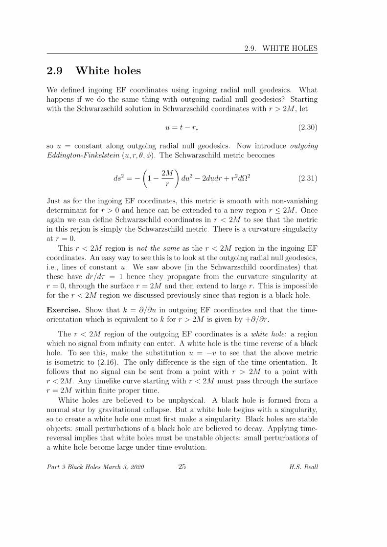
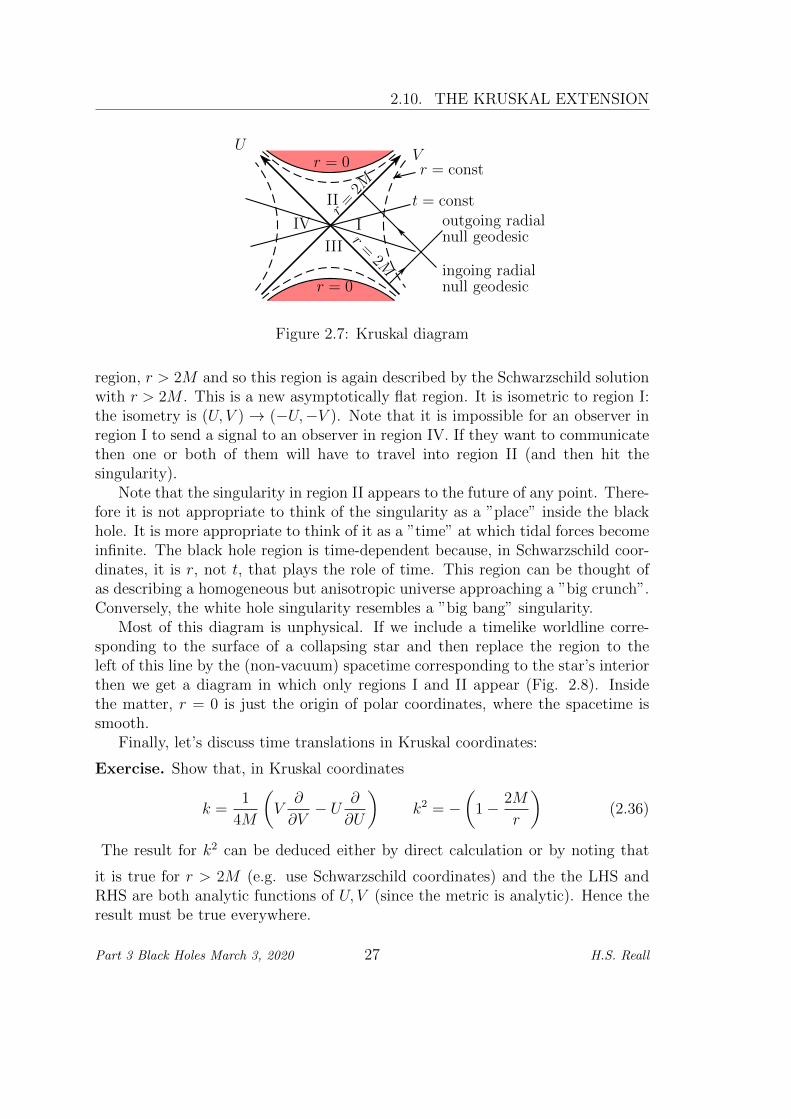
Let’s consider the surface r = 2M . Equation (2.33) implies that either U = 0or V = 0. Hence KS coordinates reveal that r = 2M is actually two surfaces, thatintersect at U = V = 0. Similarly, the curvature singularity at r = 0 correspondsto UV = 1, a hyperbola with two branches. This information can be summarizedon the Kruskal diagram of Fig. 2.7.
One should think of ”time” increasing in the vertical direction on this diagram.Radial null geodesics are lines of constant U or V , i.e., lines at 45 to the horizontal.This diagram has four regions. Region I is the region we started in, i.e., theregion r > 2M of the Schwarzschild solution. Region II is the black hole that wediscovered using ingoing EF coordinates (note that these coordinates cover regionsI and II of the Kruskal diagram), Region III is the white hole that we discoveredusing outgoing EF coordinates. And region IV is an entirely new region. In this
Part 3 Black Holes March 3, 2020 26 H.S. Reall
2.10. THE KRUSKAL EXTENSION
I
UV
II
III
IV
t = const
r=
2M
r=
2M
ingoing radialnull geodesic
outgoing radialnull geodesic
r = 0
r = 0
r = const
Figure 2.7: Kruskal diagram
region, r > 2M and so this region is again described by the Schwarzschild solutionwith r > 2M . This is a new asymptotically flat region. It is isometric to region I:the isometry is (U, V ) → (−U,−V ). Note that it is impossible for an observer inregion I to send a signal to an observer in region IV. If they want to communicatethen one or both of them will have to travel into region II (and then hit thesingularity).
Note that the singularity in region II appears to the future of any point. There-fore it is not appropriate to think of the singularity as a ”place” inside the blackhole. It is more appropriate to think of it as a ”time” at which tidal forces becomeinfinite. The black hole region is time-dependent because, in Schwarzschild coor-dinates, it is r, not t, that plays the role of time. This region can be thought ofas describing a homogeneous but anisotropic universe approaching a ”big crunch”.Conversely, the white hole singularity resembles a ”big bang” singularity.
Most of this diagram is unphysical. If we include a timelike worldline corre-sponding to the surface of a collapsing star and then replace the region to theleft of this line by the (non-vacuum) spacetime corresponding to the star’s interiorthen we get a diagram in which only regions I and II appear (Fig. 2.8). Insidethe matter, r = 0 is just the origin of polar coordinates, where the spacetime issmooth.
Finally, let’s discuss time translations in Kruskal coordinates:
Exercise. Show that, in Kruskal coordinates
k =1
4M
(V
∂
∂V− U ∂
∂U
)k2 = −
(1− 2M
r
)(2.36)
The result for k2 can be deduced either by direct calculation or by noting that
it is true for r > 2M (e.g. use Schwarzschild coordinates) and the the LHS andRHS are both analytic functions of U, V (since the metric is analytic). Hence theresult must be true everywhere.
Part 3 Black Holes March 3, 2020 27 H.S. Reall

CHAPTER 2. THE SCHWARZSCHILD BLACK HOLE
UVr = 0
r = 0(origin of polar
r = 2MI
II
coordinates)
interiorof star
Figure 2.8: Kruskal diagram for gravitational collapse. The region to the left ofthe shaded region is not part of the spacetime.
k is timeline in regions I and IV, spacelike in regions II and III, and null (orzero) where r = 2M i.e. where U = 0 or V = 0. The orbits (integral curves)of k on a Kruskal diagram are shown in Fig. 2.9. Note that the sets U = 0and V = 0 are fixed (mapped into themselves) by k and that k = 0 on the”bifurcation 2-sphere” U = V = 0. Hence points on the latter are also fixed by k.
U V
I
II
III
IV
Figure 2.9: Orbits of k in Kruskal spacetime.
Part 3 Black Holes March 3, 2020 28 H.S. Reall

2.11. EINSTEIN-ROSEN BRIDGE
2.11 Einstein-Rosen bridge
Recall equation (2.34): in region I we have V/U = −et/(2M). Hence a surface ofconstant t in region I is a straight line through the origin in the Kruskal diagram.These extend naturally into region IV (see Fig. 2.7). Let’s investigate the geometryof these hypersurfaces. Define a new coordinate ρ by
r = ρ+M +M2
4ρ(2.37)
Given r, there are two possible solutions for ρ (see Fig. 2.10). We choose ρ > M/2
r
ρ
2M
M/2
Figure 2.10: Area-radius function r as a function of isotropic radial coordinate ρ.
in region I and 0 < ρ < M/2 in region IV. The Schwarzschild metric in isotropiccoordinates (t, ρ, θ, φ) is then (exercise)
ds2 = −(1−M/(2ρ))2
(1 +M/(2ρ))2dt2 +
(1 +
M
2ρ
)4 (dρ2 + ρ2dΩ2
)(2.38)
The transformation ρ → M2/(4ρ) is an isometry that interchanges regions I andIV. Of course the above metric is singular at ρ = M/2 but we know this is just acoordinate singularity. Now consider the metric of a surface of constant t:
ds2 =
(1 +
M
2ρ
)4 (dρ2 + ρ2dΩ2
)(2.39)
This metric is non-singular for ρ > 0. It defines a Riemannian 3-manifold withtopology R×S2 (where R is parameterized by ρ). Its geometry can be visualized byembedding the surface into 4d Euclidean space (examples sheet 1). If we suppressthe θ direction, this gives the diagram shown.
Part 3 Black Holes March 3, 2020 29 H.S. Reall

CHAPTER 2. THE SCHWARZSCHILD BLACK HOLE
I
IV
S2
ρ→∞
ρ→ 0
The geometry has two asymptotically flatregions (ρ → ∞ and ρ → 0) connected by a”throat” with minimum radius 2M at ρ = M/2.A surfaces of constant t in the Kruskal space-time is called an ”Einstein-Rosen bridge”.
2.12 Extendibility
Definition. A spacetime (M, g) is extendibleif it is isometric to a proper subset of anotherspacetime (M′, g′). The latter is called an extension of (M, g).
(In GR we require that the spacetime manifold M is connected so both M andM ′ should be connected in this definition.)
For example, let (M, g) denote the Schwarzschild solution with r > 2M andlet (M′, g′) denote the Kruskal spacetime. Then M is a subset of M′ (i.e. regionI). If we define a map to take a point ofM to the corresponding point ofM′ thenthis is just the identity map in region I, which is obviously an isometry.
The Kruskal spacetime (M′, g′) is inextendible (not extendible). It is a ”maxi-mal analytic extension” of (M, g).
2.13 Singularities
We say that the metric is singular in some basis if its components are not smooth orits determinant vanishes. A coordinate singularity can be eliminated by a changeof coordinates (e.g. r = 2M in the Schwarzschild spacetime). These are unphys-ical. However, if it is not possible to eliminate the bad behaviour by a change ofcoordinates then we have a physical singularity. We have already seen an exampleof this: a scalar curvature singularity, where some scalar constructed from theRiemann tensor blows up, cannot be eliminated by a change of coordinates andhence is physical. It is also possible to have more general curvature singularities forwhich no scalar constructed from the Riemann tensor diverges but, nevertheless,there exists no chart in which the Riemann tensor remains finite.
Not all physical singularities are curvature singularities. For example considerthe manifold M = R2, introduce plane polar coordinates (r, φ) (so φ ∼ φ + 2π)and define the 2d Riemannian metric
g = dr2 + λ2r2dφ2 (2.40)
where λ > 0. The metric determinant vanishes at r = 0. If λ = 1 then this isjust Euclidean space in plane polar coordinates, so we can convert to Cartesian
Part 3 Black Holes March 3, 2020 30 H.S. Reall

2.13. SINGULARITIES
coordinates to see that r = 0 is just a coordinate singularity, i.e., g can be smoothlyextended to r = 0. But consider the case λ 6= 1. In this case, let φ′ = λφ to obtain
g = dr2 + r2dφ′2
(2.41)
which is locally isometric to Euclidean space and hence has vanishing Riemanntensor (so there is no curvature singularity at r = 0). However, it is not globallyisometric to Euclidean space because the period of φ′ is 2πλ. Consider a circler = ε. This has
circumference
radius=
2πλε
ε= 2πλ (2.42)
which does not tend to 2π as ε→ 0. Recall that any smooth Riemannian manifoldis locally flat, i.e., one recovers results of Euclidean geometry on sufficiently smallscales (one can introduce normal coordinates to show this). The above result showsthat this is not true for small circles centred on r = 0. Hence the above metriccannot be smoothly extended to r = 0. This is an example of a conical singularity.
A problem in defining singularities is that they are not ”places”: they do notbelong to the spacetime manifold because we define spacetime as a pair (M, g)where g is a smooth Lorentzian metric. For example, r = 0 is not part of theKruskal manifold. Similarly, in the example just discussed if we want a smoothRiemannian manifold then we must take M = R2\(0, 0) so that r = 0 is not a pointof M . But in both of these examples, the existence of the singularity implies thatsome geodesics cannot be extended to arbitrarily large affine parameter becausethey ”end” at the singularity. It is this property that we will use to define whatwe mean by ”singular”.
First we must eliminate a trivial case, corresponding to the possibility of ageodesic ending simply because we haven’t taken the range of its parameter to belarge enough. Recall that a curve is a smooth map γ : (a, b) → M . Sometimes acurve can be extended, i.e., it is part of a bigger curve. If this happens then thefirst curve will have an endpoint, which is defined as follows.
Definition. p ∈ M is a future endpoint of a future-directed causal curve γ :(a, b) → M if, for any neighbourhood O of p, there exists t0 such that γ(t) ∈ Ofor all t > t0. We say that γ is future-inextendible if it has no future endpoint.Similary for past endpoints and past inextendibility. γ is inextendible if it is bothfuture and past inextendible.
For example, let (M, g) be Minkowski spacetime. Let γ : (−∞, 0) → Mbe γ(t) = (t, 0, 0, 0). Then the origin is a future endpoint of γ. However, ifwe instead let (M, g) be Minkowski spacetime with the origin deleted then γ isfuture-inextendible.
Part 3 Black Holes March 3, 2020 31 H.S. Reall

CHAPTER 2. THE SCHWARZSCHILD BLACK HOLE
Definition. A geodesic is complete if an affine parameter for the geodesic extendsto ±∞. A spacetime is geodesically complete if all inextendible causal geodesicsare complete.
For example, Minkowski spacetime is geodesically complete, as is the spacetimedescribing a static spherical star. However, the Kruskal spacetime is geodesicallyincomplete because some geodesics have r → 0 in finite affine parameter andhence cannot be extended to infinite affine parameter. A similar definition appliesto Riemannian manifolds.
A spacetime that is extendible will also be geodesically incomplete. But in thiscase, it is clear that the incompleteness arises because we are not considering ”thewhole spacetime”. So we will regard a spacetime as singular if it is geodesicallyincomplete and inextendible. This is the case for the Kruskal spacetime.
Part 3 Black Holes March 3, 2020 32 H.S. Reall

Chapter 3
The initial value problem
In the next chapter we will explain why GR predicts that black holes necessarilyform under certain circumstances. To do this, we need to understand the initialvalue problem for GR.
3.1 Predictability
Definition. Let (M, g) be a time-orientable spacetime. A partial Cauchy surfaceΣ is a hypersurface for which no two points are connected by a causal curve inM . The future domain of dependence of Σ, denoted D+(Σ), is the set of p ∈ Msuch that every past-inextendible causal curve through p intersects Σ. The pastdomain of dependence, D−(Σ), is defined similarly. The domain of dependence ofΣ is D(Σ) = D+(Σ) ∪D−(Σ).
D(Σ) is the region of spacetime in which one can determine what happensfrom data specified on Σ. For example, any causal geodesic (i.e. free particleworldline) in D(Σ) must intersect Σ at some point p. The geodesic is determineduniquely by specifying its tangent vector (velocity) at p. More generally, solutionsof hyperbolic partial differential equations are uniquely determined in D(Σ) byinitial data prescribed on Σ.
Here, by ”hyperbolic partial differential equations” we mean second order par-tial differential equations for a set of tensor fields T (i)ab...
cd... (i = 1, . . . N) for whichthe equations of motion take the form
gef∇e∇fT(i)ab...
cd... = . . . (3.1)
where the RHS is a tensor that depends smoothly on the metric and its derivatives,and linearly on the fields T (j) and their first derivatives, but not their second orhigher derivatives. The Klein-Gordon equation is of this form, as are the Maxwellequations when written using a vector potential Aa in Lorenz gauge.
33

CHAPTER 3. THE INITIAL VALUE PROBLEM
For example, let Σ be the positive x-axis in 2d Minkowski spacetime (M, g)(figure 3.1). D+(Σ) is the set of points with 0 ≤ t < x, D−(Σ) is the set of pointswith −x < t ≤ 0. The boundary of D(Σ) is the pair of null rays t = ±x for x > 0.Let Σ′ be the entire x-axis. This gives D(Σ′) = M .
t = xt
x
D+(Σ)
D−(Σ)
Σ
t = −x
Figure 3.1: The regions D±(Σ)
Consider the wave equation ∇a∇aψ = −∂2t ψ + ∂2
xψ = 0 in this spacetime.Specifying the initial data (ψ, ∂tψ) on Σ determines the solution uniquely in D(Σ).Specifying initial data on Σ′ determines the solution uniquely throughout M . Twosuch solutions whose initial data agrees on the subset Σ of Σ′ will agree withinD(Σ) but differ on M\D(Σ).
This is true in general: if D(Σ) 6= M then solutions of hyperbolic equationswill not be uniquely determined in M\D(Σ) by data on Σ. Given only this data,there will be infinitely many different solutions on M which agree within D(Σ).
Definition. A spacetime (M, g) is globally hyperbolic if it admits a Cauchy surface:a partial Cauchy surface Σ such that M = D(Σ).
(If Σ is not a Cauchy surface then the past/future boundary of D(Σ) is calledthe past/future Cauchy horizon. We will define it more precisely later.)
Hence a globally hyperbolic spacetime is one in which one can predict whathappens everywhere from data on Σ. Minkowski spacetime is globally hyperbolice.g. a surface of constant t is a Cauchy surface. Other examples are the theKruskal spacetime and the spacetime describing spherically symmetric gravita-tional collapse:
Part 3 Black Holes March 3, 2020 34 H.S. Reall

3.2. EXTRINSIC CURVATURE
To obtain an example of a spacetime which is not globally hyperbolic, delete theorigin from 2d Minkowski spacetime (the cross in Fig. 3.1). For any partial Cauchysurface Σ, there will be some inextendible causal curves which don’t intersect Σbecause they ”end” at the origin.
The following theorem is proved in Wald:
Theorem. Let (M, g) be globally hyperbolic. Then (i) there exists a global timefunction: a map t : M → R such that −(dt)a (normal to surfaces of constant t)is future-directed and timelike (ii) surfaces of constant t are Cauchy surfaces, andthese all have the same topology Σ (iii) the topology of M is R× Σ.
Exercise. Show that U + V is a global time function in the Kruskal spacetime.
Since the surface U + V = 0 is an Einstein-Rosen bridge, it follows that Σ hastopology R× S2 in this case. The topology of M is R2 × S2.
xi(p)
p
t = 0
If (M, g) is globally hyperbolic then we canperform a 3 + 1 split (”Arnowitt-Deser-Misner(ADM) decomposition”) of spacetime as fol-lows. Let t be a time function. Introduce co-ordinates xi (i = 1, 2, 3) on the Cauchy surfacet = 0. Pick an everywhere timelike vector fieldT a. Given p ∈M , consider the integral curve ofT a through p. This intersects the surface t = 0at a unique point. Let xi(p) be the coordinates of this point. This defines functionsxi : M → R. We use (t, xi) as our coordinate chart. It is conventional to use thefollowing notation for the metric components:
ds2 = −N2dt2 + hij(dxi +N idt)(dxj +N jdt) (3.2)
where N(t, x) is called the lapse function (sometimes denoted α) and N i(t, x) theshift vector (sometimes denoted βi). The metric on a surface of constant t ishij(t, x).
3.2 Extrinsic curvature
In GR, not only do we need to determine the metric tensor but we also need todetermine the spacetime on which this tensor is defined. So it is not obvious whatconstitutes a suitable set of initial data for solving Einstein’s equation. However,it seems likely that we will want to prescribe data on an “initial” hypersurfaceΣ which should correspond to a “moment of time”. This we interpret as therequirement that Σ should be a spacelike hypersurface:
Definition. A hypersurface Σ is spacelike if its normal 1-form na is everywhere
Part 3 Black Holes March 3, 2020 35 H.S. Reall

CHAPTER 3. THE INITIAL VALUE PROBLEM
timelike. (A vector Xa is tangent to Σ iff naXa = 0, which implies that Xa is
spacelike.)
What data should be prescribed on Σ? Since the Einstein equation, like theKlein-Gordon equation, is second order in derivatives, one would expect that pre-scribing the spacetime metric and the “time derivative of the metric” on Σ shouldbe enough. In fact, it turns out that we do not need to prescribe a full spacetimemetric tensor on Σ, but only a Riemannian metric hab describing the intrinsic ge-ometry of Σ, obtained from the spacetime metric by pull-back. A notion of “timederivative of the metric” on Σ is provided by the extrinsic curvature tensor of Σ,which we will now introduce. First we let na be the normal 1-form to Σ, which weassume to have unit norm:
nana = −1 (3.3)
We now define the projection tensor onto Σ as
hab = δab + nanb (3.4)
Note that hab = gab+nanb is symmetric which means that it doesn’t matter whetherwe write hab or hab . If Xa and Y a are tangent to Σ then habX
aY b = gabXaY b, so
hab can be interpreted as the metric induced on Σ (the pull-back of gab to Σ). Thisis sometimes called the first fundamental form of Σ.
It is easy to check that
habnb = 0 hach
cb = hab (3.5)
which shows that hab is a projection onto Σ. We can decompose any vector on Σas
Xa = δabXb = habX
b − nanbXb ≡ Xa‖ +Xa
⊥ (3.6)
where Xa‖ = habX
b is tangent to Σ and Xa⊥ = −nbXbna is normal to Σ.
Let Na be normal to Σ at p and consider parallel transport of Na along a curvein Σ with tangent vector Xa, i.e., Xb∇bNa = 0. Does Na remain normal to Σ? Toanswer this, let Y a be another vector tangent to Σ so Y aNa = 0 at p. Considerhow Y aNa varies along the curve: X(Y aNa) = Xb∇b(Y
aNa) = NaXb∇bY
a. SoY aNa vanishes along the curve iff the RHS vanishes. So if parallel transport withinΣ preserves the property of being normal to Σ then (∇XY )⊥ = 0 for any X, Ytangent to Σ. The converse is also true. This motivates the following:
Definition. Up to now, na has been defined defined only on Σ so first extendit to a neighbourhood of Σ in an arbitrary way (with unit norm). The extrinsiccurvature tensor (also called the second fundamental form) Kab is defined at p ∈ Σ
by K(X, Y ) = −na(∇X‖Y‖
)awhere X, Y are vector fields on M .
Part 3 Black Holes March 3, 2020 36 H.S. Reall

3.2. EXTRINSIC CURVATURE
Lemma.
Kab = hcahdb∇cnd (3.7)
and Kab is independent of how na is extended.
Proof. The RHS of the definition of K(X, Y ) is
−ndXc‖∇cY
d‖ = Xc
‖Yd‖ ∇cnd = hcaX
ahdbYb∇cnd (3.8)
where we used ndYd‖ = 0 in the first equality. The final expression is linear in Xa
and Y b so the result follows. To demonstrate that the result is independent of howna is extended, consider a different extension n′a, and let ma = n′a − na so ma = 0on Σ. Then, on Σ,
XaY b (K ′ab −Kab) = Xc‖Y
d‖ ∇cmd = ∇X‖(Y
d‖ md) = X‖(Y
d‖ md) = 0 (3.9)
where the second equality uses ma = 0 on Σ and the final equality follows becauseit is the derivative along a curve tangent to Σ, along which ma = 0.
Remark. nb∇cnb = (1/2)∇c(nbnb) = 0 because nbn
b = −1. Hence we can alsowrite
Kab = hca∇cnb (3.10)
Lemma. Kab = Kba.
Proof. Let Σ be a surface of constant f with df 6= 0 on Σ. Recall a result fromsection 1.3: on Σ we have na = g(df)a for some function g chosen to make naa unit covector. We can extend na to a neighbourhood of Σ using this formula.We now have ∇cnd = g∇c∇df + (∇cg)g−1nd and so Kab = ghcah
db∇c∇df , which is
symmetric.
Lemma. Kab is related to the Lie derivative of hab along na by
Kab =1
2Lnhab (3.11)
Proof. Examples sheet 2.
This equation explains why Kab can be interpreted as “the time derivative ofthe metric on Σ.”
Part 3 Black Holes March 3, 2020 37 H.S. Reall

CHAPTER 3. THE INITIAL VALUE PROBLEM
3.3 The Gauss-Codacci equations
A tensor at p ∈ Σ is invariant under the projection hab if
T a1...ar b1...bs = ha1c1 . . . harcrh
d1b1. . . hdsbsT
c1...crd1...ds (3.12)
Tensors at p which are invariant under projection can be identified with tensorsdefined on the submanifold Σ, at p and vice-versa. (See Hawking and Ellis formore details on this correspondence.)
Proposition. A covariant derivative D on Σ can be defined by projection of thecovariant derivative on M : for any tensor obeying (3.12) we define
DaTb1...br
c1...cs = hdahb1e1. . . hbrerh
f1c1. . . hfscs∇dT
e1...erf1...fs (3.13)
Lemma. D is the Levi-Civita connection associated to the metric hab on Σ:Dahbc = 0 and D is torsion-free.
Proof. ∇ahbc = nc∇anb+nb∇anc. Acting with the projections kills both terms. Toprove the torsion-free property, let f : Σ→ R and extend to a function f : M → R.
DaDbf = hcahdb∇c (hed∇ef) = hcah
eb∇c∇ef +
(hcah
db∇ch
ed
)∇ef (3.14)
The first term is symmetric (because ∇ is torsion-free). The second term involves
hcahdb∇ch
ed = gefhcah
db∇chdf = gefhcah
dbnf∇cnd = neKab (3.15)
which is also symmetric on a, b. Hence DaDbf is symmetric so D is torsion-free.We can now calculate the Riemann tensor associated to D, which measures the
intrinsic curvature of Σ. The following result shows that this can be written interms of the Riemann tensor of ∇ and the extrinsic curvature of Σ.
Proposition. Denote the Riemann tensor associated to Da on Σ as R′abcd. This
is given by Gauss’ equation:
R′abcd = haeh
fbh
gch
hdR
efgh − 2K[c
aKd]b (3.16)
Proof. Let Xa be tangent to Σ. The Ricci identity for D is
R′abcdX
b = 2D[cDd]Xa (3.17)
Let’s calculate the RHS
DcDdXa = hech
fdh
ag∇e (DfX
g)
= hechfdh
ag∇e
(hhfh
gi∇hX
i)
= hechhdh
ai∇e∇hX
i + hechfdh
ai
(∇eh
hf
)∇hX
i + hechhdh
ag (∇eh
gi )∇hX
i
= hechfdh
ag∇e∇fX
g +Kcdhai n
h∇hXi +Kc
anihhd∇hX
i (3.18)
Part 3 Black Holes March 3, 2020 38 H.S. Reall

3.3. THE GAUSS-CODACCI EQUATIONS
where we used (3.15) in the final two terms. The final term can be written
Kcahhd∇h(niX
i)−KcaX ihhd∇hni = −Kc
aXbhibhhd∇hni = −Kc
aKbdXb (3.19)
where we used X i = hibXb because Xa is tangent to Σ. We can now plug (3.18) into
(3.17): the second term on the RHS drops out when we antisymmetrize, leaving
R′abcdX
b = 2he[chfd]h
ag∇e∇fX
g − 2K[caKd]bX
b (3.20)
The first term can be written
2hechfdh
ag∇[e∇f ]X
g = hechfdh
agR
ghefX
h = hechfdh
agh
hbR
ghefX
b (3.21)
where we used the Ricci identity for ∇ in the first equality and the fact that Xa
is parallel to Σ in the second. Moving everything to the LHS now gives(R′abcd − hech
fdh
agh
hbR
ghef + 2K[c
aKd]b
)Xb = 0 (3.22)
The expression in brackets is invariant under projection onto Σ and hence can beidentified with a tensor on Σ. Xb is an arbitrary vector parallel to Σ. It followsthat the expression in brackets must vanish. The result follows upon relabellingdummy indices.Lemma. The Ricci scalar of Σ is
R′ = R + 2Rabnanb −K2 +KabKab (3.23)
where K ≡ Kaa.
Proof. R′ = hbdR′cbcd (since hbd can be identified with the inverse metric on Σ).
Now use Gauss’ equation.
Proposition. (Codacci’s equation).
DaKbc −DbKac = hdahebh
fcn
gRdefg (3.24)
Proof.
DaKbc = hdahgbh
fc∇dKgf
= hdahgbh
fc∇d
(heg∇enf
)= hdah
gbh
fch
eg∇d∇enf + hdah
gbh
fc (∇dh
eg)∇enf
= hdahebh
fc∇d∇enf +Kabn
ehfc∇enf (3.25)
where we used (3.15) in the final line. Antisymmetrizing on a, b now gives
2D[aKb]c = 2hd[aheb]h
fc∇d∇enf = 2hdah
ebh
fc∇[d∇e]nf = hdah
ebh
fcRfgden
g (3.26)
Part 3 Black Holes March 3, 2020 39 H.S. Reall

CHAPTER 3. THE INITIAL VALUE PROBLEM
The result follows using Rdefg = Rfgde.
Lemma.
DaKab −DbK = hcbRcdn
d (3.27)
Proof. Contract Codacci’s equation with hac.
Some people refer to equation (3.27) as Codacci’s equation.
3.4 The constraint equations
Consider the “normal-normal” component of the Einstein equation, i.e., contractGab = 8πTab with nanb. On the LHS we get
Gabnanb = Rabn
anb +1
2R =
1
2
(R′ −KabKab +K2
)(3.28)
where we have used (3.23) in the final step. Therefore we have
R′ −KabKab +K2 = 16πρ (3.29)
where ρ ≡ Tabnanb is the matter energy density measured by an observer with
4-velocity na. R′ is determined by the metric on Σ, i.e., by hab. This equationreveals that we are not free to specify hab and Kab arbitrarily on Σ: they must berelated by this equation, which is called the Hamiltonian constraint.
Now consider the “normal-tangential” components of the Einstein equation bycontracting it with na and then projecting onto Σ:
8πhbaTbcnc = hbaGbcn
c = hbaRbcnc (3.30)
Using (3.27) we have
DbKba −DaK = 8πhbaTbcn
c (3.31)
Note that the RHS is (8π times) minus the momentum density measured by anobserver with 4-velocity na. The LHS of this equation involves only the metric onΣ and Kab so this is another constraint equation, called the momentum constraint.
The constraint equations involve the metric hab on Σ and its “time-derivative”Kab = (1/2)Lnhab. The remaining components of the Einstein equation, i.e.,those tangential to Σ, involve second time derivatives of hab. More precisely, theyinvolve LnLnhab. These components are evolution equations, which determine howto evolve the initial data “forward in time”.
Part 3 Black Holes March 3, 2020 40 H.S. Reall

3.5. THE INITIAL VALUE PROBLEM IN GR
3.5 The initial value problem in GR
Initial data for Einstein’s equation consists of a triple (Σ, hab, Kab) where (Σ, hab)is a Riemannian 3-manifold and Kab is a symmetric tensor. The idea is that Σcorresponds to a spacelike hypersurface in spacetime, hab is the pull-back of thespacetime metric to Σ, and Kab is the extrinsic curvature tensor of Σ, i.e., the“rate of change” of the metric on Σ. The initial data is not completely free: theEinstein equation implies that it must satisfy the constraint equations.
The following result is of fundamental significance in GR:
Theorem (Choquet-Bruhat & Geroch 1969). Let (Σ, hab, Kab) be initial datasatisfying the vacuum Hamiltonian and momentum constraints (i.e. equations(3.29,3.31) with vanishing RHS). Then there exists a unique (up to diffeomor-phism) spacetime (M, gab), called the maximal Cauchy development of (Σ, hab, Kab)such that (i) (M, gab) satisfies the vacuum Einstein equation; (ii) (M, gab) is glob-ally hyperbolic with Cauchy surface Σ; (iii) The induced metric and extrinsiccurvature of Σ are hab and Kab respectively; (iv) Any other spacetime satisfying(i),(ii),(iii) is isometric to a subset of (M, gab).
Analogous theorems exist in the non-vacuum case for suitable matter e.g. aperfect fluid or tensor fields whose equations of motion are hyperbolic partialdifferential equations (e.g. Maxwell field, scalar field, perfect fluid).
It is possible that the maximal Cauchy development (M, gab) is extendible, i.e.,isometric to a proper subset of another spacetime (M ′, g′ab). By the above theorem,Σ cannot be a Cauchy surface for (M ′, g′ab). Instead we will have M = D(Σ) ⊂M ′,and the boundaries of D(Σ) in M ′ will be future/past Cauchy horizons. If thishappens then we cannot predict physics in M ′\D(Σ) from the initial data on Σ.In particular, we cannot say determine the metric g′ab in M ′\D(Σ): there will beinfinitely possible solutions of the vacuum Einstein equation that are consistentwith the initial data on Σ. Let’s look at some examples for which this happens.
First consider initial data given by a surface Σ = (x, y, z) : x > 0 with flat3-metric δµν and vanishing extrinsic curvature. The maximal development of thisinitial data is the region |t| < x of Minkowski spacetime, which is extendible.Outside this region, we cannot predict the spacetime, in particular it need not beflat. In this example we could have anticipated that the maximal developmentwould be extendible because the initial data is extendible (to x ≤ 0). If we aregiven initial conditions only in part of space then we do not expect to be able topredict the entire spacetime.
Now consider the Schwarzschild solution with M < 0:
ds2 = −(
1 +2|M |r
)dt2 +
(1 +
2|M |r
)−1
dr2 + r2dΩ2 (3.32)
Part 3 Black Holes March 3, 2020 41 H.S. Reall

CHAPTER 3. THE INITIAL VALUE PROBLEM
This solution has a curvature singularity at r = 0 but no event horizon. Let(Σ, hab, Kab) be the data on a surface t = 0 in this spacetime (in fact Kab = 0).In this case, (Σ, hab) is inextendible. However, viewed as a Riemannian manifold,(Σ, hab) is not geodesically complete because some of its geodesics have r → 0 infinite affine parameter. So in this case, the initial data is ”singular”.
The resulting maximal development is not the whole M < 0 Schwarzschildspacetime. This is because some inextendible causal curves do not intersect Σ.For example, consider an outgoing radial null geodesic, which satisfies
dt
dr=
(1 +
2|M |r
)−1
=r
r + 2|M |≈ r
2|M |at small r (3.33)
hence t ≈ t0 + r2/(4|M |) at small r so t has a finite limit t0 as r → 0. So thisnull geodesic emerges from the singularity at time t0 and then has t > t0. Hence ift0 > 0 then this geodesic does not intersect Σ so Σ is not a Cauchy surface for thefull spacetime. One can show that the boundary of D(Σ) is given precisely by thoseradial null geodesics which have t0 = 0, i.e., they ”emerge from the singularity onΣ”: see Fig. 3.2.
r
t
D+(Σ)
D−(Σ)
Figure 3.2: Domain of dependence of t = 0 surface in negative M Schwarzschildgeometry.
We emphasize that the solution outside D(Σ) is not determined by the initialdata on Σ. The data on Σ does not predict that the solution outside D(Σ) mustcoincide with the M < 0 Schwarzschild solution. This is just one possibilityamongst infinitely many alternatives. These alternatives cannot be sphericallysymmetric because of Birkhoff’s theorem.
Part 3 Black Holes March 3, 2020 42 H.S. Reall

3.6. ASYMPTOTICALLY FLAT INITIAL DATA
t
y
xΣ
D(Σ)
In this case, the extendibility of the maximal development arises because theinitial data is singular (not geodesically complete) and one ”can’t predict whatcomes out of a singularity”. Henceforth we will restrict to initial data which isgeodesically complete (and therefore also inextendible).
Even when (Σ, hab) is geodesically complete, the maximal development may beextendible. For example, let Σ be the hyperboloid −t2 + x2 + y2 + z2 = −1 witht < 0 in Minkowski spacetime:
Take hab to be the induced metric and Kab the extrinsic curvature of thissurface. Clearly there are inextendible null curves in Minkowski spacetime whichdo not intersect Σ. The maximal development of the initial data on Σ is theinterior of the past light cone through the origin in Minkowsi spacetime. In thiscase, the maximal development is extendible because the initial data surface is”asymptotically null”, which enables ”information to arrive from infinity”.
3.6 Asymptotically flat initial data
To avoid all of these problems, we will restrict to geodesically complete initial datawhich is ”asymptotically flat” in the sense that, at large distance, it looks like a sur-face of constant t in Minkowski spacetime. (Recall that such surfaces are Cauchysurfaces for Minkowski spacetime.) We also want to allow for the possibility ofhaving several asymptotically flat regions, as in the Kruskal spacetime.
Definition. (a) An initial data set (Σ, hab, Kab) is an asymptotically flat end if(i) Σ is diffeomorphic to R3\B where B is a closed ball centred on the originin R3; (ii) if we pull-back the R3 coordinates to define coordinates xi on Σ thenhij = δij +O(1/r) and Kij = O(1/r2) as r →∞ where r =
√xixi (iii) derivatives
of the latter expressions also hold e.g. hij,k = O(1/r2) etc.(b) An initial data set is asymptotically flat with N ends if it is the union of a
compact set with N asymptotically flat ends.
(If matter fields are present then these should also decay at a suitable rate at
Part 3 Black Holes March 3, 2020 43 H.S. Reall

CHAPTER 3. THE INITIAL VALUE PROBLEM
large r.)For example, in the (M > 0) Schwarzschild solution consider the surface Σ =
t = constant, r > 2M. On examples sheet 2 it is shown that this data is anasymptotically flat end. Of course this initial data is not geodesically complete(since it stops at r = 2M). But now consider the Kruskal spacetime. Then Σcorresponds to part of an Einstein-Rosen bridge. The full Einstein-Rosen bridge isasymptotically flat with 2 ends. This is because it is the union of the bifurcationsphere U = V = 0 (a compact set) with two copies of the asymptotically flat endjust discussed (one in region I and one in region IV).
3.7 Strong cosmic censorship
For geodesically complete, asymptotically flat, initial data it would be very disturb-ing if the maximal Cauchy development were extendible. It would imply that GRsuffers from a lack of determinism (predictability). The strong cosmic censorshipconjecture asserts that this does not happen:
Strong cosmic censorship conjecture (Penrose). Let (Σ, hab, Kab) be ageodesically complete, asymptotically flat (with N ends), initial data set for thevacuum Einstein equation. Then generically the maximal Cauchy development ofthis initial data is inextendible.
This conjecture is known to be correct for initial data which is sufficientlyclose to initial data for Minkowski spacetime. For such data, a theorem of Christ-doulou and Klainerman (1994) asserts that the resulting spacetime ”settles down toMinkowski spacetime at late time”. In more physical terms, it says that Minkowskispacetime is stable against small gravitational perturbations. The spacetime hasno Cauchy horizon so strong cosmic censorship is true for such initial data.
The word ”generically” is included because of known counter-examples. Laterwe will discuss charged and rotating black hole solutions and find that they exhibita Cauchy horizon (for a geodesically complete, asymptotically flat initial data set)inside the black hole. However, this is believed to be unstable in the sense thatan arbitrarily small perturbation of this initial data has an inextendible maximaldevelopment. More formally, if one introduces some measure on the space ofgeodesically complete, asymptotically flat, initial data, strong cosmic censorshipasserts that the maximal development is inextendible except for a set of initialdata of measure zero.
The above conjecture can be extended to include matter. We need to assumethat the matter is such that the Choquet-Bruhat-Geroch theorem applies, as willbe the case if the matter fields satisfy hyperbolic equations of motion. We alsorestrict to matter that is “physical” in the sense that it has positive energy density
Part 3 Black Holes March 3, 2020 44 H.S. Reall

3.7. STRONG COSMIC CENSORSHIP
and does not travel faster than light. We do this by imposing the dominant energycondition (to be discussed later). This condition is satisfied by all “normal” matter.One also has to deal with the fact that some types of matter (e.g. a perfect fluid)can form singularities (shocks) even in the absence of gravity and so the conjectureis most straightforward to formulate for matter that doesn’t do this e.g. a Maxwellfield or Klein-Gordon field.
Proving the strong cosmic censorship conjecture, and the related weak cosmiccensorship conjecture, is one of the main goals of mathematical relativity.
Part 3 Black Holes March 3, 2020 45 H.S. Reall

CHAPTER 3. THE INITIAL VALUE PROBLEM
Part 3 Black Holes March 3, 2020 46 H.S. Reall

Chapter 4
The singularity theorem
We have seen how spherically symmetric gravitational collapse results in the forma-tion of a singularity. But maybe this is just a consequence of spherical symmetry.For example, in Newtonian theory, spherically symmetric collapse of a ball of mat-ter produces a “singularity”, i.e., infinite density at the origin. But this does nothappen without spherical symmetry. In this case, the singularity is non-generic:a tiny perturbation (breaking spherical symmetry) of the initial state results in a“bouncing” solution without a singularity. Could the same be true in GR? No.In this chapter we will discuss the Penrose singularity theorem, which shows thatsingularities are a generic prediction of GR.
4.1 Null hypersurfaces
Definition. A null hypersurface is a hypersurface whose normal is everywherenull.
Example. Consider surfaces of constant r in the Schwarzschild spacetime. The1-form n = dr is normal to such surfaces. Using ingoing Eddington-Finkelsteincoordinates, the inverse metric is
gµν =
0 1 0 01 1− 2M
r0 0
0 0 1r2
00 0 0 1
r2 sin2 θ
(4.1)
hence
n2 ≡ gµνnµnν = grr = 1− 2M
r(4.2)
47

CHAPTER 4. THE SINGULARITY THEOREM
so the surface r = 2M is a null hypersurface. Since nµ = gµνnν = gµr we have
na|r=2M =
(∂
∂v
)a(4.3)
Let na be normal to a null hypersurface N . Then any (non-zero) vector Xa
tangent to the hypersurface obeys naXa = 0 which implies that either Xa is
spacelike or Xa is parallel to na. In particular, note that na is tangent to thehypersurface. Hence, on N , the integral curves of na lie within N .
Proposition. The integral curves of na are null geodesics. These are called thegenerators of N .
Proof. Let N be given by an equation f = constant for some function f withdf 6= 0 on N . Then we have n = hdf for some function h. Let N = df . Theintegral curves of na and Na are the same up to a choice of parameterization.
Then since N is null we have that NaNa = 0 on N . Hence the function NaNa
is constant on N which implies that the gradient of this function is normal to N :
∇a
(N bNb
)|N = 2αNa (4.4)
for some function α on N . Now we also have ∇aNb = ∇a∇bf = ∇b∇af = ∇bNa.So the LHS above is 2N b∇aNb = 2N b∇bNa. Hence we have
N b∇bNa|N = αNa (4.5)
which is the geodesic equation for a non-affinely parameterized geodesic. Hence,on N , the integral curves of Na (and therefore also na) are null geodesics.
Example. In the Kruskal spacetime, let N = dU which is null everywhere (gUU =0) and normal to a family of null hypersurfaces (U = constant), which gives
N b∇bNa = N b∇b∇aU = N b∇a∇bU = N b∇aNb = (1/2)∇a(N2) = 0 (4.6)
so in this case Na is tangent to affinely parameterized null geodesics. Raising anindex gives (exercise)
Na = − r
16M3er/(2M)
(∂
∂V
)a(4.7)
Now let N be the surface U = 0. Since r = 2M on N we see that Na is aconstant multiple of ∂/∂V . Hence V is an affine parameter for the generators ofN . Similarly U is an affine parameter for the generators of the null hypersurfaceV = 0.
Part 3 Black Holes March 3, 2020 48 H.S. Reall

4.2. GEODESIC DEVIATION
4.2 Geodesic deviation
You encountered the geodesic deviation equation in the GR course. Recall thefollowing definitions:
Definition. A 1-parameter family of geodesics is a map γ : I × I ′ → M where Iand I ′ both are open intervals in R, such that (i) for fixed s, γ(s, λ) is a geodesicwith affine parameter λ (so s is the parameter that labels the geodesic); (ii) themap (s, λ) 7→ γ(s, λ) is smooth and one-to-one with a smooth inverse. This impliesthat the family of geodesics forms a 2d surface Σ ⊂M .
Let Ua be the tangent vector to the geodesics and Sa to be the vector tangentto the curves of constant t, which are parameterized by s (see Fig. 4.1). In
λ = const
S
S
UU U
s = const
Figure 4.1: 1-parameter family of geodesics
a chart xµ, the geodesics are specified by xµ(s, λ) with Sµ = ∂xµ/∂s. Hencexµ(s + δs, λ) = xµ(s, λ) + δsSµ(s, λ) +O(δs2). Therefore (δs)Sa points from onegeodesic to an infinitesimally nearby one in the family. We call Sa a deviationvector.
In a neighbourhood of Σ we can use coordinates (s, λ, y1, y2) for suitable y1, y2.This gives a coordinate chart in which S = ∂/∂s and U = ∂/∂λ on Σ. Hence Sa
and Ua commute:
[S, U ] = 0 ⇔ U b∇bSa = Sb∇bU
a (4.8)
Recall that this implies that Sa satisfies the geodesic deviation equation
U c∇c(Ub∇bS
a) = RabcdU
bU cSd (4.9)
Given an affinely parameterized geodesic γ with tangent Ua, a solution Sa of thisequation along γ is called a Jacobi field.
Part 3 Black Holes March 3, 2020 49 H.S. Reall

CHAPTER 4. THE SINGULARITY THEOREM
4.3 Geodesic congruences
Definition. Let U ⊂ M be open. A geodesic congruence in U is a family ofgeodesics such that exactly one geodesic passes through each p ∈ U .
We will consider a congruence for which all the geodesics are of the same type(timelike or spacelike or null). Then by normalizing the affine parameter we canarrange that the tangent vector Ua satisfies U2 = ±1 (in the spacelike or timelikecase) or U2 = 0 (in the null case) everywhere.
Now consider a 1-parameter family of geodesics belonging to a congruence.Write (4.8) as
U b∇bSa = Ba
bSb (4.10)
whereBa
b = ∇bUa (4.11)
measures the failure of Sa to be parallelly transported along the geodesic withtangent Ua. Note that
BabU
b = 0 (4.12)
because Ua is tangent to affinely parameterized geodesics. Note also that
UaBab =
1
2∇b(U
2) = 0 (4.13)
because we’ve arranged that U2 is constant throughout U . This implies that
U · ∇(U · S) = (U · ∇Ua)Sa + UaU · ∇Sa = UaBabSb = 0 (4.14)
using the geodesic equation and (4.10). Hence U ·S is constant along any geodesicin the congruence.
Now recall that, even after normalising so that U2 ∈ ±1, 0, the affine pa-rameter is not uniquely defined because we are free to shift it by a constant. Wecan choose this constant to be different on different geodesics, i.e., it can dependon s: λ′ = λ− a(s) is just as good an affine parameter as λ. But this changes thedeviation vector to (exercise)
S′a ≡ Sa +
da
dsUa (4.15)
Hence S′a is a deviation vector pointing to the same geodesic as Sa:
Now U · S ′ = U · S + (da/ds)U2 so in the spacelike or timelike case, we can fix
Part 3 Black Holes March 3, 2020 50 H.S. Reall

4.4. NULL GEODESIC CONGRUENCES
this ”gauge freedom” by choosing a(s) so that U · S = 0 at some point on eachgeodesic (e.g. λ = 0). Since U ·S is constant along each geodesic, this implies thatU · S = 0 everywhere.
4.4 Null geodesic congruences
In the null case, the above procedure does not work because U · S ′ = U · S.Instead we fix the gauge freedom as follows. Pick a spacelike hypersurface Σwhich intersects each geodesic once. Let Na be a vector field defined on Σ obeyingN2 = 0 and N · U = −1 on Σ. Now extend Na off Σ by parallel transport alongthe geodesics: U · ∇Na = 0. This implies N2 = 0 and N · U = −1 everywhere(proof: exercise). In summary, we’ve constructed a vector field such that
N2 = 0 U ·N = −1 U · ∇Na = 0 (4.16)
We can now decompose any deviation vector uniquely as
Sa = αUa + βNa + Sa (4.17)
whereU · S = N · S = 0 (4.18)
which implies that Sa is spacelike (or zero). Note that U · S = −β hence β isconstant along each geodesic. So we can write a deviation vector Sa the sum ofa part αUa + Sa orthogonal to Ua and a part βNa that is parallelly transportedalong each geodesic.
An important case is when the congruence contains the generators of a nullhypersurface N and we are interested only in the behaviour of these generators.In this case, if we pick a 1-parameter family of geodesics contained within N thenthe deviation vector Sa will be tangent to N and hence obey U · S = 0 (since Ua
is normal to N ) i.e. β = 0.Note that we can write
Sa = P ab S
b (4.19)
whereP ab = δab +NaUb + UaNb (4.20)
is a projection (i.e. P ab P
bc = P a
c ) of the tangent space at p onto T⊥, the 2d spaceof vectors at p orthogonal to Ua and Na. Since Ua and Na are both parallellytransported, so is P a
b :U · ∇P a
b = 0 (4.21)
Proposition. A deviation vector for which U · S = 0 satisfies U · ∇Sa = BabS
b
where Bab = P a
c BcdP
db .
Part 3 Black Holes March 3, 2020 51 H.S. Reall

CHAPTER 4. THE SINGULARITY THEOREM
Proof. U · ∇Sa = U · ∇(P ac S
c) = P ac U · ∇Sc = P a
c BcdS
d = P ac B
cdP
de S
e usingU ·S = 0 and Bc
dUd = 0 in the final step. Finally we can use P 2 = P to write the
RHS as P ac B
cdP
db P
beS
e = BabS
b.
4.5 Expansion, rotation and shear
Note that Bab can be regarded as a matrix that acts on the 2d space T⊥. To
understand its geometrical interpretation, it is useful to divide it into its trace,traceless symmetric, and antisymmetric parts as follows:
Definition. The expansion, shear and rotation of the null geodesic congruenceare
θ = Baa σab = B(ab) −
1
2Pabθ, ωab = B[ab] (4.22)
This implies
Bab =
1
2θP a
b + σab + ωab (4.23)
Exercise. Show that θ = gabBab = ∇aUa.
This shows that the expansion is independent of the choice of Na, i.e., it is anintrinsic property of the congruence. Scalar invariants of the rotation and shear(e.g. ωabω
ab or the eigenvalues of σab) are also independent of the choice of Na.
Proposition. If the congruence contains the generators of a (null) hypersurfaceN then ωab = 0 on N . Conversely, if ωab = 0 everywhere then Ua is everywherehypersurface orthogonal (i.e. orthogonal to a family of null hypersurfaces).
Proof. The definition of B and U ·B = B · U = 0 implies
Bbc = Bb
c + U bNdBdc + UcB
bdN
d + U bUcNdBdeN
e (4.24)
Using this, we haveU[aωbc] = U[aBbc] = U[aBbc] (4.25)
since the extra terms drop out of the antisymmetrization. Now using the definitionof Bab we have
U[aωbc] = U[a∇cUb] = −1
6(U ∧ dU)abc (4.26)
If Ua is normal to N then U ∧ dU = 0 on N and hence, on N ,
0 = U[aωbc] =1
3(Uaωbc + Ubωca + Ucωab) (4.27)
Contracting this with Na gives ωbc = 0 on N (using U · N = −1 and ω · N =0). Conversely, if ω = 0 everywhere then (4.26) implies that U is hypersurface-orthogonal using Frobenius’ theorem.
Part 3 Black Holes March 3, 2020 52 H.S. Reall

4.6. EXPANSION AND SHEAR OF A NULL HYPERSURFACE
expansion shear
λ = λ0
λ = λ1
Figure 4.2: Effects of expansion and shear on the generators of a null hypersurface.
4.6 Expansion and shear of a null hypersurface
Assume that we have a congruence which includes the generators of a null hyper-surface N . The generators of N have ω = 0. To understand how these generatorsbehave, restrict attention to deviation vectors tangent to N (i.e. consider a 1-parameter family of generators of N ). Consider the evolution of the generators ofN as a function of affine parameter λ, as shown in Fig. 4.2.
Qualitatively: expansion θ corresponds to neighbouring generators movingapart (if θ > 0) or together (if θ < 0). Shear corresponds to geodesics movingapart in one direction, and together in the orthogonal direction whilst preservingthe cross-sectional area.
We can make this more precise by introducing Gaussian null coordinates nearN as follows (see Fig. 4.3). Pick a spacelike 2-surface S within N and let yi
(i = 1, 2) be coordinates on this surface. Assign coordinates (λ, yi) to the pointaffine parameter distance λ from S along the generator of N (with tangent Ua)which intersects the surface S at the point with coordinates yi. Now we havecoordinates (λ, yi) on N such that the generators are lines of constant yi andUa = (∂/∂λ)a.
Let V a be a null vector field on N satisfying V · ∂/∂yi = 0 and V · U = 1.Assign coordinates (r, λ, yi) to the point affine parameter distance r along the nullgeodesic which starts at the point on N with coordinates (λ, yi) and has tangentvector V a there.
Part 3 Black Holes March 3, 2020 53 H.S. Reall

CHAPTER 4. THE SINGULARITY THEOREM
N
(λ, yi)
S
yi
V(r, λ, yi)
Figure 4.3: Construction of Gaussian null coordinates near a null hypersurface N .
This defines a coordinate chart in a neighbourhood of N such that N is atr = 0, with U = ∂/∂λ on N , and ∂/∂r is tangent to affinely parameterized nullgeodesics. The latter implies that grr = 0 everywhere.
Exercise. Use the geodesic equation for ∂/∂r to show grµ,r = 0.
At r = 0 we have grλ = V ·U = 1 (as V = ∂/∂r onN ) and gri = V ·(∂/∂yi) = 0.Since grµ is independent of r, these results are valid for all r. We also know thatgλλ = 0 at r = 0 (as Ua is null) and gλi = 0 at r = 0 (as ∂/∂yi is tangent to Nand hence orthogonal to Ua). So we can write gλλ = rF and gλi = rhi for somesmooth functions F , hi. Therefore the metric takes the form
ds2 = 2drdλ+ rFdλ2 + 2rhidλdyi + hijdy
idyj (4.28)
(We note that F must vanish at r = 0. To see this, we use the fact that the curves λ 7→ (0, λ, yi),
for constant yi are affinely parameterized null geodesics: the generators of N . For these the
only-non vanishing component of the geodesic equation is the r component. This reduces to
∂r(rF ) = 0 Hence F = 0 at r = 0 so we can write F = rF for some smooth function F .)
On N the metric isg|N = 2drdλ+ hijdy
idyj (4.29)
so Uµ = (0, 1, 0, 0) on N implies that Uµ = (1, 0, 0, 0) on N . Now U ·B = B ·U = 0implies that Br
µ = Bµλ = 0. We saw above that θ = Bµ
µ. Hence on N we have
θ = Bii = ∇iU
i = ∂iUi + ΓiiµU
µ = Γiiλ =1
2giµ (gµi,λ + gµλ,i − giλ,µ) (4.30)
In the final expression, note that the form of the metric on N implies that giµ is
Part 3 Black Holes March 3, 2020 54 H.S. Reall

4.7. TRAPPED SURFACES
non-vanishing only when µ = j, and that gij = hij (the inverse of hij) hence on N
θ =1
2hij (gji,λ + gjλ,i − giλ,j) =
1
2hijhij,λ =
∂λ√h√h
(4.31)
where we used giλ = 0 on N and defined h = dethij. Hence we have
∂
∂λ
√h = θ
√h (4.32)
From (4.29),√h is the area element on a surface of constant λ within N , so θ
measures the rate of increase of this area element with respect to affine parameteralong the geodesics.
4.7 Trapped surfaces
Consider a 2d spacelike surface S, i.e., a 2d submanifold for which all tangentvectors are spacelike. For any p ∈ S there will be precisely two future-directednull vectors Ua
1 and Ua2 orthogonal to S (up to the freedom to rescale Ua
1 and Ua2 ).
If we assume that S is orientable then Ua1 and Ua
2 can be defined continuously overS. This defines two families of null geodesics which start on S and are orthogonalto S (with the freedom to rescale Ua corresponding to the freedom to rescale theaffine parameter). These null geodesics form two null hypersurfaces N1 and N2.In simple situations, these correspond to the set of ”outgoing” and ”ingoing” lightrays that start on S. Consider a null congruence that contains the generators ofNi. By the proposition above, we will have ωab = 0 on N1 and N2.
Example. Let S be a 2-sphere U = U0, V = V0 in the Kruskal spacetime. Bysymmetry, the generators of Ni will be radial null geodesics, as shown in Fig. 4.4.
Hence Ni must be surfaces of constant U or constant V with generators tangentto dU and dV respectively. We saw above that dU and dV correspond to affineparameterization. Raising an index, equation (4.7) gives
Ua1 = rer/2M
(∂
∂V
)aUa
2 = rer/2M(∂
∂U
)a(4.33)
where we have discarded an overall constant and fixed the sign so that Ua1 and Ua
2
are future-directed. (∂/∂U and ∂/∂V are future-directed because they are globallynull and hence define time-orientations. In region I they both give the same timeorientation as the one defined by ka.) We can now calculate the expansion of these
Part 3 Black Holes March 3, 2020 55 H.S. Reall
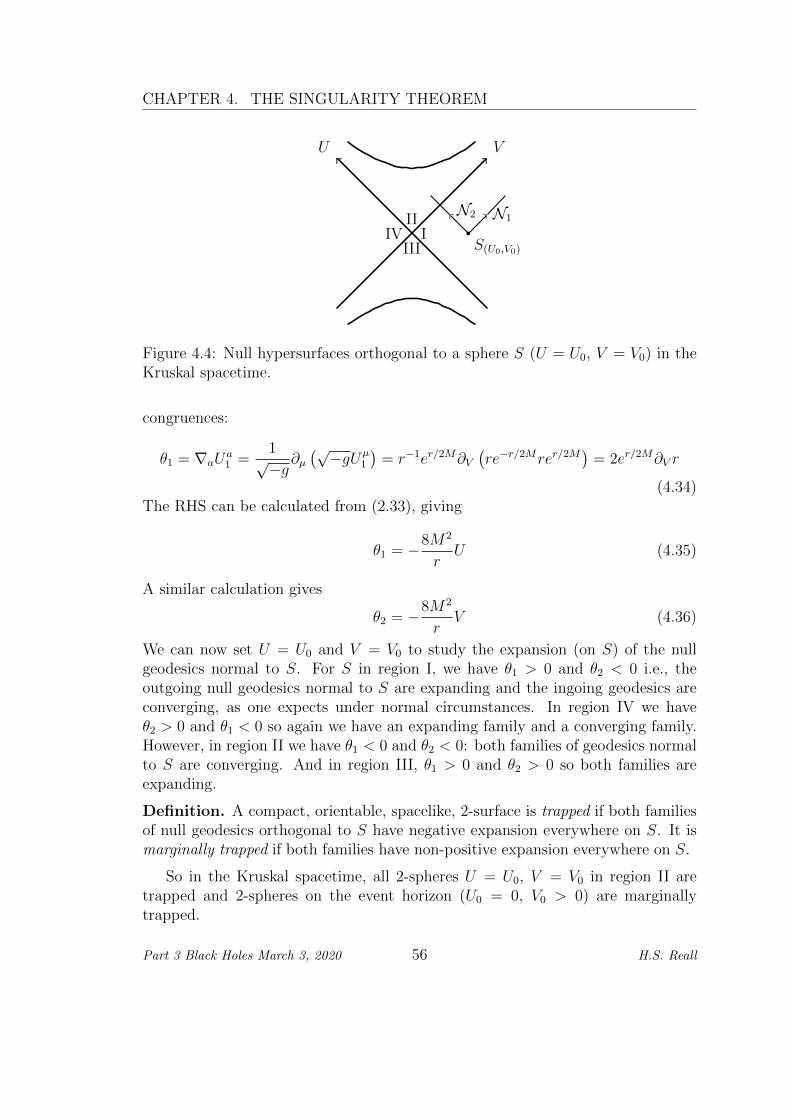
CHAPTER 4. THE SINGULARITY THEOREM
VU
III
IIIIV
S(U0,V0)
N1N2
Figure 4.4: Null hypersurfaces orthogonal to a sphere S (U = U0, V = V0) in theKruskal spacetime.
congruences:
θ1 = ∇aUa1 =
1√−g
∂µ(√−gUµ
1
)= r−1er/2M∂V
(re−r/2Mrer/2M
)= 2er/2M∂V r
(4.34)The RHS can be calculated from (2.33), giving
θ1 = −8M2
rU (4.35)
A similar calculation gives
θ2 = −8M2
rV (4.36)
We can now set U = U0 and V = V0 to study the expansion (on S) of the nullgeodesics normal to S. For S in region I, we have θ1 > 0 and θ2 < 0 i.e., theoutgoing null geodesics normal to S are expanding and the ingoing geodesics areconverging, as one expects under normal circumstances. In region IV we haveθ2 > 0 and θ1 < 0 so again we have an expanding family and a converging family.However, in region II we have θ1 < 0 and θ2 < 0: both families of geodesics normalto S are converging. And in region III, θ1 > 0 and θ2 > 0 so both families areexpanding.
Definition. A compact, orientable, spacelike, 2-surface is trapped if both familiesof null geodesics orthogonal to S have negative expansion everywhere on S. It ismarginally trapped if both families have non-positive expansion everywhere on S.
So in the Kruskal spacetime, all 2-spheres U = U0, V = V0 in region II aretrapped and 2-spheres on the event horizon (U0 = 0, V0 > 0) are marginallytrapped.
Part 3 Black Holes March 3, 2020 56 H.S. Reall

4.8. RAYCHAUDHURI’S EQUATION
4.8 Raychaudhuri’s equation
Let’s determine how the expansion evolves along the geodesics of a null geodesiccongruence.
Proposition (Raychaudhuri’s equation).
dθ
dλ= −1
2θ2 − σabσab + ωabωab −RabU
aU b (4.37)
Proof. From the definition of θ we have
dθ
dλ= U · ∇
(Ba
bPba
)= P b
aU · ∇Bab = P b
aUc∇c∇bU
a (4.38)
Now commute derivatives using the definition of the Riemann tensor:
dθ
dλ= P b
aUc(∇b∇cU
a +RadcbU
d)
= P ba [∇b(U
c∇cUa)− (∇bU
c)(∇cUa)] + P b
aRadcbU
cUd
= −BcbP
baB
ac −RcdU
cUd (4.39)
where we used the geodesic equation and, in the final term, the antisymmetry ofthe Riemann tensor allows us to replace P b
a with δba. Finally (exercise) we canrewrite the first term so that
dθ
dλ= −Bc
aBac −RabU
aU b (4.40)
The result then follows by using (4.23).Similar calculations give equations governing the evolution of shear and rota-
tion.
4.9 Energy conditions
Raychaudhuri’s equation involves the Ricci tensor, which is related to the energy-momentum tensor of matter via the Einstein equation. We will want to consideronly ”physical” matter, which implies that the energy-momentum tensor shouldsatisfy certain conditions. For example, an observer with 4-velocity ua would mea-sure an ”energy-momentum current” ja = −T abub. We would expect ”physicallyreasonable” matter not to move faster than light, so this current should be non-spacelike. This motivates:
Dominant energy condition. −T abV b is a future-directed causal vector (orzero) for all future-directed timelike vectors V a.
Part 3 Black Holes March 3, 2020 57 H.S. Reall
CHAPTER 4. THE SINGULARITY THEOREM
For matter satisfying the dominant energy condition, if Tab is zero in someclosed region S of a spacelike hypersurface Σ then Tab will be zero within D+(S).(See Hawking and Ellis for a proof.)
Example. Consider a massless scalar field
Tab = ∂aΦ∂bΦ−1
2gab(∂Φ)2 (4.41)
Let
ja = −T abV b = −(V · ∂Φ)∂aΦ +1
2V a(∂Φ)2 (4.42)
then, for timelike V a,
j2 =1
4V 2((∂Φ)2
)2 ≤ 0 (4.43)
so ja is indeed causal or zero. Now consider
V · j = −(V · ∂Φ)2 +1
2V 2(∂Φ)2 = −1
2(V · ∂Φ)2 +
1
2V 2
(∂Φ− V · ∂Φ
V 2V
)2
(4.44)
the final expression in brackets is orthogonal to V a and hence must be spacelikeor zero, so its norm is non-negative. We then have V · j ≤ 0 using V 2 < 0. Henceja is future-directed (or zero).
A less restrictive condition requires only that the energy density measured byall observers is positive:
Weak energy condition. TabVaV b ≥ 0 for any causal vector V a.
A special case of this is
Null energy condition. TabVaV b ≥ 0 for any null vector V a.
The dominant energy condition implies the weak energy condition, which im-plies the null energy condition. Another energy condition is
Strong energy condition. (Tab − (1/2)gabTcc )V aV b ≥ 0 for all causal vectors
V a.
Using the Einstein equation, this is equivalent to RabVaV b ≥ 0, or ”gravity
is attractive”. Despite its name, the strong energy condition does not imply theweak energy condition. The strong energy condition is needed to prove some ofthe singularity theorems, but the dominant energy condition is the most importantphysically. For example, our universe appears to contain a positive cosmologicalconstant. This violates the strong energy condition but respects the dominantenergy condition.
Part 3 Black Holes March 3, 2020 58 H.S. Reall

4.10. CONJUGATE POINTS
4.10 Conjugate points
Lemma. In a spacetime satisfying Einstein’s equation with matter obeying thenull energy condition, the generators of a null hypersurface satisfy
dθ
dλ≤ −1
2θ2 (4.45)
Proof. Consider the RHS of Raychaudhuri’s equation. The generators of a null
hypersurface have ω = 0. Vectors in T⊥ are all spacelike, so the metric restrictedto T⊥ is positive definite. Hence σabσab ≥ 0. Einstein’s equation gives RabU
aU b =8πTabU
aU b because Ua is null. Hence the null energy condition implies RabUaU b ≥
0. The result follows from Raychaudhuri’s equation.
Corollary. If θ = θ0 < 0 at a point p on a generator γ of a null hypersurface thenθ → −∞ along γ within an affine parameter distance 2/|θ0| provided γ extendsthis far.
Proof. Let λ = 0 at p. Equation (4.45) implies
d
dλθ−1 ≥ 1
2(4.46)
Integrating gives θ−1 − θ−10 ≥ λ/2, which can be rearranged to give
θ ≤ θ0
1 + λθ0/2(4.47)
if θ0 < 0 then the RHS → −∞ as λ→ 2/|θ0|.
Definition. Points p, q on a geodesic γ are conjugate if there exists a Jacobi field(i.e. a solution of the geodesic deviation equation) along γ that vanishes at p andq but is not identically zero.
Roughly speaking, if p and q are conjugate then there exist multiple infinitesi-mally nearby geodesics which pass through p and q:
The following results are proved in Hawking and Ellis:
Part 3 Black Holes March 3, 2020 59 H.S. Reall

CHAPTER 4. THE SINGULARITY THEOREM
Theorem 1. Consider a null geodesic congruence which includes all of the nullgeodesics through p (this congruence is singular at p). If θ → −∞ at a point q ona null geodesic γ through p then q is conjugate to p along γ.
Theorem 2. Let γ be a causal curve with p, q ∈ γ. Then there does not exist asmooth 1-parameter family of causal curves γs connecting p, q with γ0 = γ and γstimelike for s > 0 (i.e. γ cannot be smoothly deformed to a timelike curve) if, andonly if, γ is a null geodesic with no point conjugate to p along γ between p and q.
For example, consider the 3d spacetime R× S2 with metric
ds2 = −dt2 + dΩ2 (4.48)
Null geodesics emitted from the south pole at time t = 0 (the spacetime point p)all reconverge at the north pole at time t = π (spacetime point r)
Such geodesics correspond to great circles of S2. r is conjugate to p along anyof these geodesics. If q lies beyond r along one of these geodesics then by deformingthe great circle into a shorter path one can travel from p to q with velocity lessthan that of light hence there exists a timelike curve from p to q.
Now consider the case in which we have a 2d spacelike surface S. As discussedabove, we can introduce two future-directed null vector fields Ua
1 , Ua2 on S that
are normal to S and consider the null geodesics which have one of these vectors astheir tangent on S. These generate a null hypersurface N . Let p be a point on ageodesic γ in this family. We say that p is conjugate to S if there exists a Jacobifield along γ that vanishes at p and, on S, is tangent to S. If p is conjugate to Sthen, roughly speaking, infinitesimally nearby geodesics normal to S intersect atp.
The analogue of theorem 1 in this case is: p is conjugate to S if θ → −∞ at palong one of the geodesics just discussed, in a congruence containing the generatorsof N . (We saw earlier that θ depends only in the geodesics in N and not on howthe other geodesics in the congruence are chosen.)
Part 3 Black Holes March 3, 2020 60 H.S. Reall

4.11. CAUSAL STRUCTURE
4.11 Causal structure
Definition. Let (M, g) be a time-orientable spacetime and U ⊂M . The chrono-logical future of U , denoted I+(U), is the set of points of M which can be reachedby a future-directed timelike curve starting on U . The causal future of U , denotedJ+(U), is the union of U with the set of points of M which can be reached bya future-directed causal curve starting on U . The chronological past I−(U) andcausal past J−(U) are defined similarly.
For example, let q be a point in Minkowski spacetime. Then I+(p) is the setof points strictly inside the future light cone of p and J+(p) is the set of points onor inside the future light cone of p, including p itself.
Next we need to review some basic topological ideas. A subset S of M is openif, for any point p ∈ S, there exists a neighbourhood V of p (i.e. a set of pointswhose coordinates in some chart are a neighbourhood of the coordinates of p) suchthat V ⊂ S. Small deformations of timelike curves remain timelike. Hence I±(U)are open subsets of M .
We use an overbar to denote the closure of a set, i.e., the union of a set and itslimit points. In Minkowski spacetime, we have I±(p) = J±(p) so J±(p) are closedsets, i.e., they contain their limit points. This is not true in general e.g. let (M, g)be the spacetime obtained by deleting a point from 2d Minkowski spacetime:
In this example we see that J+(p) 6= I+(p) and J+(p) is not closed.
A point p ∈ S is an interior point if there exists a neighbourhood of p containedin S. The interior of S, denoted int(S) is the set of interior points of S. If S isopen then int(S) = S. The boundary of S is S = S\int(S). This is a topological
Part 3 Black Holes March 3, 2020 61 H.S. Reall
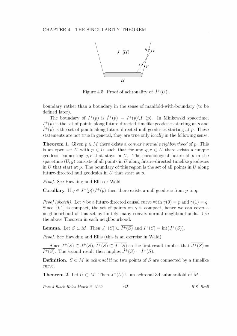
CHAPTER 4. THE SINGULARITY THEOREM
J+(U)
p
q
s
r
U
Figure 4.5: Proof of achronality of J+(U).
boundary rather than a boundary in the sense of manifold-with-boundary (to bedefined later).
The boundary of I+(p) is I+(p) = I+(p)\I+(p). In Minkowski spacetime,I+(p) is the set of points along future-directed timelike geodesics starting at p andI+(p) is the set of points along future-directed null geodesics starting at p. Thesestatements are not true in general, they are true only locally in the following sense:
Theorem 1. Given p ∈M there exists a convex normal neighbourhood of p. Thisis an open set U with p ∈ U such that for any q, r ∈ U there exists a uniquegeodesic connecting q, r that stays in U . The chronological future of p in thespacetime (U, g) consists of all points in U along future-directed timelike geodesicsin U that start at p. The boundary of this region is the set of all points in U alongfuture-directed null geodesics in U that start at p.
Proof. See Hawking and Ellis or Wald.
Corollary. If q ∈ J+(p)\I+(p) then there exists a null geodesic from p to q.
Proof (sketch). Let γ be a future-directed causal curve with γ(0) = p and γ(1) = q.Since [0, 1] is compact, the set of points on γ is compact, hence we can cover aneighbourhood of this set by finitely many convex normal neighbourhoods. Usethe above Theorem in each neighbourhood.
Lemma. Let S ⊂M . Then J+(S) ⊂ I+(S) and I+(S) = int(J+(S)).
Proof. See Hawking and Ellis (this is an exercise in Wald).
Since I+(S) ⊂ J+(S), I+(S) ⊂ J+(S) so the first result implies that J+(S) =I+(S). The second result then implies J+(S) = I+(S).
Definition. S ⊂M is achronal if no two points of S are connected by a timelikecurve.
Theorem 2. Let U ⊂M . Then J+(U) is an achronal 3d submanifold of M .
Part 3 Black Holes March 3, 2020 62 H.S. Reall

4.11. CAUSAL STRUCTURE
Proof. (See Fig. 4.5.) Assume p, q ∈ J+(U) with q ∈ I+(p). Since I+(p)is open, there exists r (near q) with r ∈ I+(p) but r /∈ J+(U). Similarly, sinceI−(r) is open, there exists s (near p) with s ∈ I−(r) and s ∈ J+(U). Hence thereexists a causal curve from U to s to r so r ∈ J+(U), which is a contradiction.Hence we can’t have q ∈ I+(p), which establishes achronality. For proof of the”submanifold” part see Wald.
For example, let M = R× S1 with the flat metric
ds2 = −dt2 + dφ2 (4.49)
where φ ∼ φ + 2π parameterizes S1 (this is a 2d version of the ”Einstein staticuniverse”). The diagram shows J+(p) (shaded). Its boundary J+(p) is a pair ofnull geodesic segments which start at p and end at q.
Note that q is a future endpoint of these geodesics. They could be extendedto the future beyond q but then they would leave J+(p). They also have a pastendpoint at p.
The next theorem characterises the behaviour of J+(U).
Theorem 3. Let U ⊂ M be closed. Then every p ∈ J+(U) with p /∈ U lies on anull geodesic λ lying entirely in J+(U) and such that λ is either past-inextendibleor has a past endpoint on U .
Proof (sketch). Since U is closed, M\U is a manifold. We will work in thismanifold. Consider a compact neighbourhood V of p and a sequence of pointspn ∈ I+(U) = int(J+(U)) with limit point p. Let λn be a timelike curve from Uto pn and let qn be the past endpoint of λn in V :
Then one can show that qn has a limit point q ∈ J+(U) and there is a causal”limit curve” λ from q to p lying in J+(U) (see Wald). We need to show λ ⊂ J+(U).
Part 3 Black Holes March 3, 2020 63 H.S. Reall

CHAPTER 4. THE SINGULARITY THEOREM
Suppose there is a point r ∈ λ such that r ∈ I+(U) = int(J+(U)). Then thereis a timelike curve γ from r′ ∈ U to r. But then we can get from r′ to r to p byfollowing γ then λ. Hence p ∈ J+(r′) but p /∈ I+(r′) (as p /∈ I+(U)) so theorem 1implies that this curve must be a null geodesic, which is a contradiction becauseit’s not null everywhere. Hence we must have λ ⊂ J+(U)− I+(U) = J+(U).
Theorem 2 tells us that J+(U) is achronal so p /∈ I+(q). Theorem 1 then tellsus that λ must be a null geodesic. Now we repeat the argument starting at q, toget a point r ∈ J+(U) with a null geodesic λ′ from r to q lying in J+(U), If λ′
were not the past extension of λ we could ”round off the corner” to construct atimelike curve from r to p, violating achronality. This argument can be repeatedindefinitely, hence λ cannot have a past endpoint in M\U .
In the case of a globally hyperbolic spacetime, this theorem can be strengthenedas follows:
Theorem 4. Let S be a 2-dimensional orientable compact spacelike submanifoldof a globally hyperbolic spacetime. Then every p ∈ J+(S) lies on a future-directednull geodesic starting from S which is orthogonal to S and has no point conjugateto S between S and p.
Finally, we can use the notation of this section to define what we mean by aCauchy horizon:
Definition. The future Cauchy horizon of a partial Cauchy surface Σ is H+(Σ) =D+(Σ)\I−(D+(Σ)). Similarly for the past Cauchy horizon H−(Σ).
We don’t define H+(Σ) simply as D+(Σ) since this includes Σ itself. However,one can show that D(Σ) = H+(Σ) ∪H−(Σ). One can also show that H± are nullhypersurfaces in the same sense as J+(U) in Theorems 2 and 3 above. (See Waldfor details.)
4.12 Penrose singularity theorem
Theorem (Penrose 1965). Let (M, g) be globally hyperbolic with a non-compact Cauchy surface Σ. Assume that the Einstein equation and the null energycondition are satisfied and that M contains a trapped surface T . Let θ0 < 0 be themaximum value of θ on T for both sets of null geodesics orthogonal to T . Then atleast one of these geodesics is future-inextendible and has affine length no greaterthan 2/|θ0|.Proof. Assume that all future inextendible null geodesics orthogonal to T haveaffine length greater than 2/|θ0|. Along any of these geodesics, we will have θ →−∞ (from the Corollary in section 4.10), and hence a point conjugate to T , withinaffine parameter no greater than 2/|θ0|.
Part 3 Black Holes March 3, 2020 64 H.S. Reall

4.12. PENROSE SINGULARITY THEOREM
Let p ∈ J+(T ), p /∈ T . From theorem 4 above, we know that p lies on afuture-directed null geodesic γ starting from T which is orthogonal to T and hasno point conjugate to T between T and p. It follows that p cannot lie beyond thepoint on γ conjugate to T on γ.
Therefore J+(T ) is a subset of the compact set consisting of the set of pointsalong the null geodesics orthogonal to T , with affine parameter less than or equalto 2/|θ0|. Since J+(T ) is closed this implies that J+(T ) is compact. Now recall(theorem 2 of section 4.11) that J+(T ) is a manifold, which implies that it can’thave a boundary. If Σ were compact this might be possible because the ”ingoing”and ”outgoing” congruences orthogonal to T might join up:
But since Σ is non-compact, this can’t happen and we’ll now reach a contra-diction as follows. Pick a timelike vector field T a (possible because our manifoldis time-orientable). By global hyperbolicity, integral curves of this vector field willintersect Σ exactly once. They will intersect J+(T ) at most once (because this setis achronal by theorem 2 of section 4.11). This defines a continuous one-to-one mapα : J+(T ) → Σ. This is a homeomorphism between J+(T ) and α(J+(T )) ⊂ Σ.Since the former is a closed set, so must be the latter. Now J+(T ) is a 3d subman-ifold hence for any p ∈ J+(T ) we can find a neighbourhood V of p in J+(T ). Thenα(V ) gives a neighbourhood of α(p) in α(J+(T )) hence the latter set is open (inΣ). Since it is both open and closed, and since Σ is connected (this follows fromconnectedness of M) we have α(J+(T )) = Σ. But this is a contradiction becausethe set on the LHS is compact (because J+(T ) is).
The formation of trapped surfaces is routinely observed in numerical simula-tions of gravitational collapse. There are also various mathematical results con-cerning the formation of trapped surfaces. The Einstein equation possesses theproperty of Cauchy stability, which implies that the solution in a compact regionof spacetime depend continuously on the initial data. In a spacetime describingspherically symmetric gravitational collapse, choose a compact region that includesa trapped surface (e.g. a 2-sphere in region II of the Kruskal diagram). Cauchystability implies that if one perturbs the initial data (breaking spherical symme-try) then the resulting spacetime will also have a trapped surface, for a small
Part 3 Black Holes March 3, 2020 65 H.S. Reall

CHAPTER 4. THE SINGULARITY THEOREM
enough initial perturbation. This shows that trapped surfaces occur generically ingravitational collapse.
A theorem due to Schoen and Yau (1983) establishes that asymptotically flatinitial data will contain a trapped surface if the energy density of matter is suffi-ciently large in a small enough region. Recently, Christodoulou (2009) has provedthat trapped surfaces can be formed dynamically, even in the absence of matterand without any symmetry assumptions, by sending sufficiently strong gravita-tional waves into a small enough region.
The above theorem implies that if the maximal development of asymptoti-cally flat initial data contains a trapped surface then this maximal development isnot geodesically complete. Such incompletness might arise because the maximaldevelopment is extendible. However, this is (generically) excluded if the strongcosmic censorship conjecture is correct. Hence it is expected that, generically,the incompleteness arises because the maximal development is singular. In fact,a different singularity theorem (due to Hawking and Penrose) eliminates the as-sumption that spacetime is globally hyperbolic (at the cost of requiring the strongenergy condition and a mild ”genericity” assumption on the spacetime curvature)and still proves existence of incomplete geodesics. So even if the maximal develop-ment is extendible then the Hawking-Penrose theorem implies that this extendedspacetime must be geodesically incomplete, i.e., singular.
Hence there are very good reasons to believe that gravitational collapse leadsto formation of a singularity. Notice that these theorems tell us nothing aboutthe nature of this singularity e.g. we do not know that it must be a curvaturesingularity as occurs in spherically symmetric collapse.
Part 3 Black Holes March 3, 2020 66 H.S. Reall

Chapter 5
Asymptotic flatness
We’ve already defined the notion of asymptotic flatness of an initial data set. Inthis chapter, we will define what it means for a spacetime to be asymptoticallyflat. We’ll then be able to define the term ”black hole”.
5.1 Conformal compactification
Given a spacetime (M, g) we can define a new metric g = Ω2g where Ω is asmooth positive function on M . We say that g is obtained from g by a conformaltransformation. The metrics g, g agree on the definitions of ”timelike”, ”spacelike”and ”null” so they have the same light cones, i.e., the same causal structure.
M
M
Ω = 0
The idea of conformal compactification is to choose Ω sothat ”points at infinity” with respect to g are at ”finitedistance” w.r.t. the ”unphysical” metric g. To do thiswe need Ω → 0 ”at infinity”. More precisely, we tryto choose Ω so that the spacetime (M, g) is extendiblein the sense we discussed previously, i.e., (M, g) is partof a larger ”unphysical” spacetime (M, g). M is then aproper subset of M with Ω = 0 on the boundary ∂M ofM in M . This boundary ∂M corresponds to ”infinity”in (M, g). It is easiest to see how this works by lookingat some examples.Minkowski spacetime
Let (M, g) be Minkowski spacetime. In spherical polars the metric is
g = −dt2 + dr2 + r2dω2 (5.1)
(We denote the metric on S2 by dω2 to avoid confusion with the conformal factor
67

CHAPTER 5. ASYMPTOTIC FLATNESS
Ω.) Define retarded and advanced time coordinates
u = t− r v = t+ r (5.2)
In what follows it will be important to keep track of the ranges of the differentcoordinates: since r ≥ 0 we have −∞ < u ≤ v <∞. The metric is
g = −dudv +1
4(u− v)2dω2 (5.3)
Now define new coordinates (p, q) by
u = tan p v = tan q (5.4)
so the range of (p, q) is finite: −π/2 < p ≤ q < π/2. This gives
g = (2 cos p cos q)−2[−4dpdq + sin2(q − p)dω2
](5.5)
”Infinity” in the original coordinates corresponds to |t| → ∞ or r → ∞. In thenew coordinates this corresponds to |p| → π/2 or |q| → π/2.
To conformally compactify this spacetime, define the positive function
Ω = 2 cos p cos q (5.6)
and letg = Ω2g = −4dpdq + sin2(q − p)dω2 (5.7)
Finally defineT = q + p ∈ (−π, π) χ = q − p ∈ [0, π) (5.8)
sog = −dT 2 + dχ2 + sin2 χdω2 (5.9)
Now dχ2+sin2 χdω2 is the unit radius round metric on S3. If we had T ∈ (−∞,∞)and χ ∈ [0, π] then g would be the metric of the Einstein static universe R× S3,given by the product of a flat time direction with the unit round metric on S3.The ESU can be visualised as an infinite cylinder, whose axis corresponds to thetime direction. In our case the restrictions on the ranges of p, q imply that M isjust a finite portion of the ESU, as shown in Fig. 5.1.
Let (M, g) denote the ESU. This is an extension of (M, g). The boundary∂M of M in M corresponds to ”infinity” in Minkowski spacetime. This consistsof (i) the points labelled i± i.e. T = ±π, χ = 0 (ii) the point labelled i0, i.e.,T = 0, χ = π (iii) a pair of null hypersurfaces I± (I is pronounced ”scri”) withequations T = ±(π − χ), which are parameterized by χ ∈ (0, π) and (θ, φ) andhence have the topology of cylinders R× S2 (since (0, π) is diffeomorphic to R).
Part 3 Black Holes March 3, 2020 68 H.S. Reall
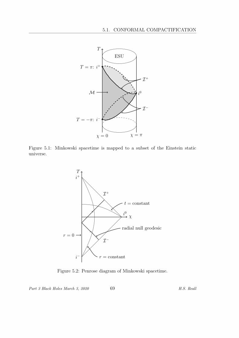
5.1. CONFORMAL COMPACTIFICATION
χ = 0
T
χ = π
T = −π: i−
T = π: i+
i0
I+
I−
ESU
M
Figure 5.1: Minkowski spacetime is mapped to a subset of the Einstein staticuniverse.
T
χ
i−
i+
i0
I−
I+
r = constant
t = constant
radial null geodesic
r = 0
Figure 5.2: Penrose diagram of Minkowski spacetime.
Part 3 Black Holes March 3, 2020 69 H.S. Reall

CHAPTER 5. ASYMPTOTIC FLATNESS
It is convenient to project the above diagram onto the (T, χ)-plane to obtainthe Penrose diagram of Minkowski spacetime shown in Fig. 5.2.
Formally, a Penrose diagram is a bounded subset of R2 endowed with a flatLorentzian metric (in this case −dT 2 + dχ2). Each point of the interior of aPenrose diagram represents an S2. Points of the boundary can represent an axisof symmetry (where r = 0) or points at ”infinity” of our original spacetime withmetric g.
Let’s understand how the geodesics of g look on a Penrose diagram. This iseasiest for radial geodesics, i.e., constant θ, φ. Remember that the causal structureof g and g is the same. Hence radial null curves of g are null curves of the flatmetric −dT 2 + dχ2, i.e., straight lines at 45. These all start at I−, pass throughthe origin, and end at I+. For this reason, I− is called past null infinity and I+
is called future null infinity. Similarly, radial timelike geodesics start i− and endat i+ so i− is called past timelike infinity and i+ is called future timelike infinity.Finally, radial spacelike geodesics start and end at i0 so i0 is called spatial infinity.
One can also plot the projection of non-radial curves onto the Penrose dia-gram. This projection makes things look ”more timelike” w.r.t. the 2d flat metric(because moving the final term in (5.9) to the LHS gives a negative contribu-tion). Hence a non-radial timelike geodesic remains timelike when projected anda non-radial null curve looks timelike when projected.
The behaviour of geodesics has an analogue for fields. Roughly speaking, mass-less radiation ”comes in from” I− and ”goes out to” I+. For example, consider amassless scalar field ψ in Minkowski spacetime, i.e., a solution of the wave equation∇a∇aψ = 0. For simplicity, assume it is spherically symmetric ψ = ψ(t, r).
Exercise. Show that the general spherically symmetric solution of the wave equa-tion in Minkowski spacetime is
ψ(t, r) =1
r(f(u) + g(v)) =
1
r(f(t− r) + g(t+ r)) (5.10)
where f and g are arbitrary functions. This is singular at r = 0 (and hence not asolution there) unless g(x) = −f(x) which gives
ψ(t, r) =1
r(f(u)− f(v)) =
1
r(F (p)− F (q)) (5.11)
where F (x) = f(tanx). If we let F0(q) denote the limiting value of rψ on I− (wherep = −π/2) then we have F (−π/2) − F (q) = F0(q) so F (q) = F (−π/2) − F0(q).Hence we can write the solution as
ψ =1
r(F0(q)− F0(p)) (5.12)
Part 3 Black Holes March 3, 2020 70 H.S. Reall
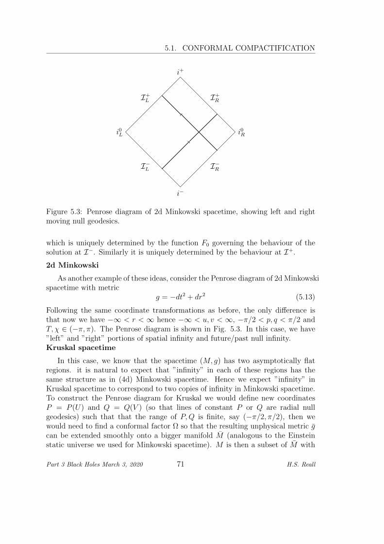
5.1. CONFORMAL COMPACTIFICATION
i0R
i+
i0L
i−
I+RI+
L
I−L I−R
Figure 5.3: Penrose diagram of 2d Minkowski spacetime, showing left and rightmoving null geodesics.
which is uniquely determined by the function F0 governing the behaviour of thesolution at I−. Similarly it is uniquely determined by the behaviour at I+.
2d Minkowski
As another example of these ideas, consider the Penrose diagram of 2d Minkowskispacetime with metric
g = −dt2 + dr2 (5.13)
Following the same coordinate transformations as before, the only difference isthat now we have −∞ < r < ∞ hence −∞ < u, v < ∞, −π/2 < p, q < π/2 andT, χ ∈ (−π, π). The Penrose diagram is shown in Fig. 5.3. In this case, we have”left” and ”right” portions of spatial infinity and future/past null infinity.Kruskal spacetime
In this case, we know that the spacetime (M, g) has two asymptotically flatregions. it is natural to expect that ”infinity” in each of these regions has thesame structure as in (4d) Minkowski spacetime. Hence we expect ”infinity” inKruskal spacetime to correspond to two copies of infinity in Minkowski spacetime.To construct the Penrose diagram for Kruskal we would define new coordinatesP = P (U) and Q = Q(V ) (so that lines of constant P or Q are radial nullgeodesics) such that that the range of P,Q is finite, say (−π/2, π/2), then wewould need to find a conformal factor Ω so that the resulting unphysical metric gcan be extended smoothly onto a bigger manifold M (analogous to the Einsteinstatic universe we used for Minkowski spacetime). M is then a subset of M with
Part 3 Black Holes March 3, 2020 71 H.S. Reall

CHAPTER 5. ASYMPTOTIC FLATNESS
III
IIIIV i0
i+i+′
i0′
i−i−′
I+I+′
I−′ I−
t = constantr = constant
r = constant
r = 0
r = 0
Figure 5.4: Penrose diagram of the Kruskal spacetime.
a boundary that has 4 components, corresponding to places where either P or Qis ±π/2. We identify these 4 components as future/past null infinity in region I,which we denote as I± and future/past null infinity in region IV, which we denoteas I±′ .
Doing this explicitly is fiddly. Fortunately we don’t need to do it: now we’veunderstood the structure of infinity we can deduce the form of the Penrose diagramfrom the Kruskal diagram. This is because both diagrams show radial null curvesas straight lines at 45. The only important difference is that ”infinity” correspondsto a boundary of the Penrose diagram. It is conventional to use the freedom inchoosing Ω to arrange that the curvature singularity at r = 0 is a horizontalstraight line in the Penrose diagram. The result is shown in Fig. 5.4.
In contrast with the conformal compactification of Minkowski spacetime, itturns out that the unphysical metric is singular at i± (and i±
′). This can be
understood because lines of constant r meet at i±, and this includes the curvaturesingularity r = 0. Less obviously, it turns out that one can’t choose Ω to make theunphysical metric smooth at i0.
Spherically symmetric collapse
The Penrose diagram for spherically symmetric gravitational collapse is easyto deduce from the form of the Kruskal diagram. It is shown in Fig. 5.5.
Part 3 Black Holes March 3, 2020 72 H.S. Reall

5.2. ASYMPTOTIC FLATNESS
r = 0
r=
0
i0
i+
I+
I−
Figure 5.5: Penrose diagram for spherically symmetric gravitational collapse.
5.2 Asymptotic flatness
An asymptotically flat spacetime is one that ”looks like Minkowski spacetime atinfinity”. In this section we will define this precisely. Infinity in Minkowski space-time consists of I±, i± and i0. However, we saw that i± are singular points in theconformal compactification of the Kruskal spacetime. Since we want to regard thelatter as asymptotically flat, we cannot include i± in our definition of asymptoticflatness. We also mentioned that i0 is not smooth in the Kruskal spacetime so wewill also not include i0. (However, it is possible to extend the definition to includei0, see Wald for details.) So we will define a spacetime to be asymptotically flat ifit has the same structure for null infinity I± as Minkowski spacetime.
First, recall that a manifold-with-boundary is defined in the same way as amanifold except that the charts are now maps φ : M → Rn/2 ≡ (x1, . . . , xn) :x1 ≤ 0. The boundary ∂M of M is defined to be the set of points which havex1 = 0 in some chart.
Definition. A time-orientable spacetime (M, g) is asymptotically flat at null in-finity if there exists a spacetime (M, g) such that
1. There exists a positive function Ω on M such that (M, g) is an extension of(M,Ω2g) (hence if we regard M as a subset of M then g = Ω2g on M).
2. Within M , M can be extended to obtain a manifold-with-boundary M ∪∂M
3. Ω can be extended to a function on M such that Ω = 0 and dΩ 6= 0 on ∂M
Part 3 Black Holes March 3, 2020 73 H.S. Reall

CHAPTER 5. ASYMPTOTIC FLATNESS
4. ∂M is the disjoint union of two components I+ and I−, each diffeomorphicto R× S2
5. No past (future) directed causal curve starting in M intersects I+ (I−)
6. I± are ”complete”. We’ll define this below.
Conditions 1,2,3 are just the requirement that there exist an appropriate con-formal compactification. The condition dΩ 6= 0 ensures that Ω has a first orderzero on ∂M , as in the examples discussed above. This is needed to ensure that thespacetime metric approaches the Minkowski metric at an appropriate rate nearI±. Conditions 4,5,6 ensure that infinity has the same structure as null infinityof Minkowski spacetime. In particular, condition 5 ensures that I+ lies ”to thefuture of M” and I− lies ”to the past of M”.
Example. Consider the Schwarzschild solution in outgoing EF coordinates (u, r, θ, φ),for which I+ corresponds to r → ∞ with finite u. Let r = 1/x with x > 0. Thisgives
g = − (1− 2Mx) du2 + 2dudx
x2+
1
x2
(dθ2 + sin2 θdφ2
)(5.14)
Hence by choosing a conformal factor Ω = x we obtain the unphysical metric
g = −x2 (1− 2Mx) du2 + 2dudx+ dθ2 + sin2 θdφ2 (5.15)
which can be smoothly extended across x = 0. The surface x = 0 is I+. It isparameterized by (u, θ, φ) and is hence diffeomorphic to R× S2. Of course we’veonly checked the above definition at I+ here. But one can do the same at I− usingingoing EF coordinates and the same conformal factor Ω = 1/r (recall that r is thesame for both coordinate charts). Hence the Schwarzschild spacetime is asymptot-ically flat at null infinity. Similarly, the Kruskal spacetime is asymptotically flat(in fact both regions I and IV are asymptotically flat).
Let’s now see how the above definition implies that the metric must approachthe Minkowski metric near I+ (of course I− is similar).
Exercise (examples sheet 2). Let ∇ denote the Levi-Civita connection of gand Rab the Ricci tensor of g. Show that on M
Rab = Rab + 2Ω−1∇a∇bΩ + gabgcd(Ω−1∇c∇dΩ− 3Ω−2∂cΩ∂dΩ
)(5.16)
We will consider the case in which (M, g) satisfies the vacuum Einstein equa-
tion. This assumption can be weakened: our results will apply also to spacetimes
Part 3 Black Holes March 3, 2020 74 H.S. Reall
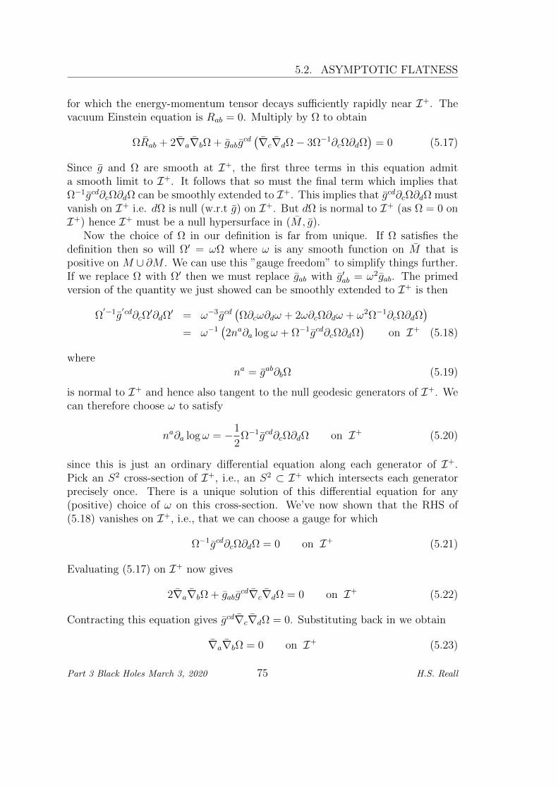
5.2. ASYMPTOTIC FLATNESS
for which the energy-momentum tensor decays sufficiently rapidly near I+. Thevacuum Einstein equation is Rab = 0. Multiply by Ω to obtain
ΩRab + 2∇a∇bΩ + gabgcd(∇c∇dΩ− 3Ω−1∂cΩ∂dΩ
)= 0 (5.17)
Since g and Ω are smooth at I+, the first three terms in this equation admita smooth limit to I+. It follows that so must the final term which implies thatΩ−1gcd∂cΩ∂dΩ can be smoothly extended to I+. This implies that gcd∂cΩ∂dΩ mustvanish on I+ i.e. dΩ is null (w.r.t g) on I+. But dΩ is normal to I+ (as Ω = 0 onI+) hence I+ must be a null hypersurface in (M, g).
Now the choice of Ω in our definition is far from unique. If Ω satisfies thedefinition then so will Ω′ = ωΩ where ω is any smooth function on M that ispositive on M ∪ ∂M . We can use this ”gauge freedom” to simplify things further.If we replace Ω with Ω′ then we must replace gab with g′ab = ω2gab. The primedversion of the quantity we just showed can be smoothly extended to I+ is then
Ω′−1g
′cd∂cΩ′∂dΩ
′ = ω−3gcd(Ω∂cω∂dω + 2ω∂cΩ∂dω + ω2Ω−1∂cΩ∂dΩ
)= ω−1
(2na∂a logω + Ω−1gcd∂cΩ∂dΩ
)on I+ (5.18)
where
na = gab∂bΩ (5.19)
is normal to I+ and hence also tangent to the null geodesic generators of I+. Wecan therefore choose ω to satisfy
na∂a logω = −1
2Ω−1gcd∂cΩ∂dΩ on I+ (5.20)
since this is just an ordinary differential equation along each generator of I+.Pick an S2 cross-section of I+, i.e., an S2 ⊂ I+ which intersects each generatorprecisely once. There is a unique solution of this differential equation for any(positive) choice of ω on this cross-section. We’ve now shown that the RHS of(5.18) vanishes on I+, i.e., that we can choose a gauge for which
Ω−1gcd∂cΩ∂dΩ = 0 on I+ (5.21)
Evaluating (5.17) on I+ now gives
2∇a∇bΩ + gabgcd∇c∇dΩ = 0 on I+ (5.22)
Contracting this equation gives gcd∇c∇dΩ = 0. Substituting back in we obtain
∇a∇bΩ = 0 on I+ (5.23)
Part 3 Black Holes March 3, 2020 75 H.S. Reall

CHAPTER 5. ASYMPTOTIC FLATNESS
(Ω, u, θ, φ)
(u, θ, φ)
na
S2 I+
Figure 5.6: Coordinates near future null infinity.
and hence
∇anb = 0 on I+ (5.24)
In particular we have
na∇anb = 0 on I+ (5.25)
so, in this gauge, na is tangent to affinely parameterized (w.r.t. g) null geodesicgenerators of I+. Furthermore, (5.24) shows that these generators have vanishingexpansion and shear.
We introduce coordinates near I+ as follows (see Fig. 5.6). In our choice ofgauge, we still have the freedom to choose ω on a S2 cross-section of I+. A standardresult is that any Riemannian metric on S2 is conformal to the unit round metricon S2. Hence we can choose ω so that the metric on our S2 induced by g (i.e. thepull-back of g to this S2) is the unit round metric. Introduce coordinates (θ, φ) onthis S2 so that the unit round metric takes the usual form dθ2 + sin2 θdφ2. Nowassign coordinates (u, θ, φ) to the point parameter distance u along the integralcurve of na through the point on this S2 with coordinates (θ, φ). This defines acoordinate chart on I+ with the property that the generators of I+ are lines ofconstant θ, φ with affine parameter u.
On I+ consider the vectors that are orthogonal (w.r.t. g) to the 2-spheres ofconstant u, i.e., orthogonal to ∂/∂θ and ∂/∂φ. Such vectors form a 2d subspace ofthe tangent space. In 2d, there are only two distinct null directions. Hence thereare two distinct null directions orthogonal to the 2-spheres of constant u. One ofthese is tangent to I+ so pick the other one, which points into M .
Consider the null geodesics whose tangent at I+ is in this direction. Extend(u, θ, φ) off I+ by defining them to be constant along these null geodesics. Finally,since dΩ 6= 0 on I+, we can use Ω as a coordinate near I+. We now have acoordinate chart (u,Ω, θ, φ) defined in a neighbourhood of I+, with I+ given byΩ = 0.
By construction we have a coordinate chart with na = ∂/∂u on I+. Hence
Part 3 Black Holes March 3, 2020 76 H.S. Reall

5.2. ASYMPTOTIC FLATNESS
nµ = δµu . But the definition of na implies ∂µΩ = gµνnν from which we deduce
guµ = δΩµ at Ω = 0. Since (u, θ, φ) don’t vary along the null geodesics pointing
into M , the tangent vector to these geodesics must be proportional to ∂/∂Ω.Since the geodesics are null we must therefore have gΩΩ = 0 for all Ω. We alsoknow that these geodesics are orthogonal to ∂/∂θ and ∂/∂φ on I+ hence we havegΩθ = gΩφ = 0 at Ω = 0.
Now consider the gauge condition (5.23). Writing this out in our coordinatechart, it reduces to
0 = ΓΩµν =
1
2gΩρ (gρµ,ν + gρν,µ − gµν,ρ) =
1
2(guµ,ν + guν,µ − gµν,u) at Ω = 0
(5.26)where we used gΩρ = gνρ(dΩ)ν = nρ = δρu. Taking µ and ν to be θ or φ, we haveguµ,ν = guν,µ = 0 so we learn that gµν,u = 0 at Ω = 0, i.e., the θ, φ components ofthe metric g on I+ don’t depend on u. Since we know that this metric is the unitround metric when u = 0, it must be the unit round metric for all u.
We have now deduced the form of the unphysical metric on I+:
g|Ω=0 = 2dudΩ + dθ2 + sin2 dφ2 (5.27)
For small Ω 6= 0, the metric components will differ from the above result by O(Ω)terms. However, by setting ν = Ω in (5.26) and taking µ to be u, θ or φ, welearn that guµ,Ω = 0 at Ω = 0 so smoothness of g implies that guµ = O(Ω2) forµ = u, θ, φ.
Finally we can write down the physical metric g = Ω−2g. It is convenient todefine a new coordinate r = 1/Ω so that I+ corresponds to r →∞. On examplessheet 2, it is shown that, after a finite shift in r, the metric can be brought to theform
g = −2dudr + r2(dθ2 + sin2 θdφ2
)+ . . . (5.28)
for large r, where the ellipsis refers to corrections that are subleading at large r.The leading terms written above are simply the metric of Minkowski spacetime. Ifone converts this to inertial frame coordinates (t, x, y, z) so that the leading ordermetric is diag(−1, 1, 1, 1) then the correction terms are all of order 1/r (exam-ples sheet 2). Hence the metric of an asymptotically flat spacetime does indeedapproach the Minkowski metric at I+.
Finally we can explain condition 6 of our definition of asymptotic flatness.Nothing in the above construction guarantees that the range of u is (−∞,∞)as it is in Minkowski spacetime. We would not want to regard a spacetime asasymptotically flat if I+ ”ends” at some finite value of u. Recall that u is theaffine parameter along the generators of I+ so if this happens then the generatorsof I+ would be incomplete. Condition 6 eliminates this possibility.
Part 3 Black Holes March 3, 2020 77 H.S. Reall

CHAPTER 5. ASYMPTOTIC FLATNESS
III
IIIIV
I+
I−
black hole
white hole
Figure 5.7: Black hole and white hole regions in the Kruskal spacetime.
Definition. I+ is complete if, in the gauge (5.23), the generators of I+ arecomplete (i.e. the affine parameter extends to ±∞). Similarly for I−.
This completeness assumption will be important when we discuss weak cosmiccensorship.
5.3 Definition of a black hole
We can now make precise our definition of a black hole as a region of an asymptot-ically flat spacetime from which it is impossible to send a signal to infinity. I+ is asubset of our unphysical spacetime (M, g) so we can define J−(I+) ⊂ M . The setof points of M that can send a signal to I+ is M ∩ J−(I+). We define the blackhole region to be the complement of this region, and the future event horizon tobe the boundary of the black hole region:
Definition. Let (M, g) be a spacetime that is asymptotically flat at null infinity.The black hole region is B = M\[M ∩ J−(I+)] where J−(I+) is defined using theunphysical spacetime (M, g). The future event horizon is H+ = B (the boundaryof B in M), equivalently H+ = M ∩ J−(I+). Similarly, the white hole region isW = M\[M ∩ J+(I−)] and the past event horizon is H− = W = M ∩ J+(I−).
One can construct examples of spacetimes with a non-empty black hole regionsimply by deleting sets of points from Minkowski spacetime. However, we caneliminate such trivial examples by restricting attention to spacetimes that are themaximal development of geodesically complete, asymptotically flat initial data.
In the Kruskal spacetime, no causal curve from region II or IV can reach I+
hence B is the union of regions II and IV (including the boundary U = 0 wherer = 2M). H+ is the surface U = 0. W is the union of regions III and IV (includingthe boundary V = 0). H− is the surface V = 0. See Fig. 5.7.
Theorems 2 and 3 of section 4.11 imply that H± are null hypersurfaces. The-orem 3 (time reversed) implies that the generators of H+ cannot have future end-
Part 3 Black Holes March 3, 2020 78 H.S. Reall

5.3. DEFINITION OF A BLACK HOLE
points. However, they can have past endpoints. This happens in the spacetimedescribing spherically symmetric gravitational collapse, with Penrose diagram:
The generators of H+ have a past endpoint at p, which is the point at whichthe black hole forms. So null generators can enter H+ but they cannot leave it.Note that the sets W and H− are empty in this spacetime.
We will need a extra technical condition to prove useful things about blackholes:
Definition. An asymptotically flat spacetime (M, g) is strongly asymptoticallypredictable if there exists an open region V ⊂ M such that M ∩ J−(I+) ⊂ V and(V , g) is globally hyperbolic.
This definition implies that (M ∩ V , g) is a globally hyperbolic subset of M .Roughly speaking, there is a globally hyperbolic region M ∩ V of spacetime con-sisting of the region not in B together with a neighbourhood of H+. It ensures thatphysics is predictable on, and outside, H+. A simple consequence of this definitionis the result that a black hole cannot bifurcate (split into two):
Theorem. Let (M, g) be strongly asymptotically predictable and let Σ1, Σ2 beCauchy surfaces for V with Σ2 ⊂ I+(Σ1). Let B be a connected component ofB ∩Σ1. Then J+(B) ∩Σ2 is contained within a connected component of B ∩Σ2.
Proof. (See Fig. 5.8.) Global hyperbolicity implies that every causal curve fromΣ1 intersects Σ2 and vice-versa. Note that J+(B) ⊂ B hence J+(B)∩Σ2 ⊂ B∩Σ2.Assume J+(B)∩Σ2 is not contained within a single connected component of B∩Σ2.Then we can find disjoint open sets O,O′ ⊂ Σ2 such that J+(B)∩Σ2 ⊂ O∪O′ withJ+(B)∩O 6= ∅, J+(B)∩O′ 6= ∅. Then B ∩ I−(O) and B ∩ I−(O′) are non-emptyand B ⊂ I−(O)∪I−(O′). Now p ∈ B cannot lie in both I−(O) and I−(O′) for thenwe could divide future-directed timelike geodesics from p into two sets accordingto whether they intersected O or O′, and hence divide the future-directed timelikevectors at p into two disjoint open sets, contradicting connectedness of the futurelight-cone at p. Hence the open sets B ∩ I−(O) and B ∩ I−(O′) are disjoint opensets whose union is B. This contradicts the connectedness of B.
Part 3 Black Holes March 3, 2020 79 H.S. Reall

CHAPTER 5. ASYMPTOTIC FLATNESS
Σ1
Σ2
B
O O′
Figure 5.8: Bifurcation of a black hole.
Figure 5.9: Penrose diagram of M < 0 Schwarzschild solution. The curvaturesingularity at r = 0 is naked.
5.4 Weak cosmic censorship
In our Penrose diagram for spherically symmetric gravitational collapse, the singu-larity at r = 0 is hidden behind the event horizon: no signal from the singularitycan reach I+. (More precisely: no inextendible incomplete causal geodesic reachesI+.) This is not true for the Kruskal spacetime, where a signal from the whitehole curvature singularity can reach I+: it is a naked singularity. Similarly, thecurvature singularity of the M < 0 Schwarzschild solution is naked: see Fig. 5.9.
The singularity theorems tell us that gravitational collapse results in the for-mation of a singularity (i.e. geodesic incompleteness). But could this singularitybe naked?
If we have a spherically symmetric collapsing star then Birkhoff’s theorem
Part 3 Black Holes March 3, 2020 80 H.S. Reall

5.4. WEAK COSMIC CENSORSHIP
tells us that the exterior of the star is given by the Schwarzschild solution, withthe same (positive) mass as the star. This gives the standard diagram for grav-itational collapse to form a black hole. However, this is just a consequence ofspherical symmetry and Birkhoff’s theorem. With spherical symmetry, the dy-namics of the gravitational field is trivial: there are no gravitational waves (andno electromagnetic waves if there is a Maxwell field).
In order to make the dynamics more interesting we will assume that the matterin our spacetime includes a scalar field. This allows us to maintain the convenienceof spherical symmetry, i.e., the use of Penrose diagrams, whilst circumventingBirkhoff’s theorem. If the scalar field is non-trivial outside the collapsing matterthen Birkhoff’s theorem doesn’t apply. We emphasize that the only reason forincluding this scalar field is to make the dynamics richer and therefore give us anidea of what is possible in the more general situation without spherical symmetry.
It is now tempting to draw the following diagram describing collapse to forma naked singularity:
(With the scalar field, we can no longer define a sharp boundary to the col-lapsing matter so the surface of the star is not precisely defined.) Imagine startingfrom initial data on Σ as shown. This data describes a collapsing star. The initialdata is geodesically complete and asymptotically flat. When the star collapses tozero size, a timelike singularity forms. This is naked because it can send a signalto I+.
This diagram is misleading. Note the presence of a future Cauchy horizonH+(Σ) which bounds the maximal development of Σ. The spacetime beyondH+(Σ) is not determined by data on Σ. Hence we cannot say what happensbeyond H+(Σ): one would need extra information (new laws of physics) to do so.So it is incorrect to draw a diagram as above. Instead we should draw just themaximal development of the initial data on Σ:
Part 3 Black Holes March 3, 2020 81 H.S. Reall

CHAPTER 5. ASYMPTOTIC FLATNESS
This spacetime does not have a singularity which can send a signal to I+.But the spacetime shown is pathological in two respects. First, even though westarted from geodesically complete, asymptotically flat initial data, the maximaldevelopment is extendible. Hence strong cosmic censorship is violated. Second,the spacetime does not satisfy our definition of asymptotic flatness. This is becauseI+ is not complete: only part of it is present. The weak cosmic censorship propertyasserts that the latter behaviour does not occur:
Conjecture (weak cosmic censorship). Let (Σ, hab, Kab) be a geodesicallycomplete, asymptotically flat, initial data set. Let the matter fields obey hyper-bolic equations and satisfy the dominant energy condition. Then generically themaximal development of this initial data is an asymptotically flat spacetime (inparticular it has a complete I+) that is strongly asymptotically predictable.
Just like strong cosmic censorship, this conjecture refers only to the maximaldevelopment, i.e., to the region of spacetime that can be predicted uniquely fromthe initial data. This conjecture captures the idea that a ”naked singularity wouldlead to an incomplete I+” without referring to any actual singularity.
The word ”generically” is included because it is known that there exist exam-ples which violate the conjecture if this word is omitted. However, such examplesare ”fine-tuned”, i.e., if one introduces an appropriate measure on the space ofinitial data then the set of data which violates the conjecture is of measure zero.For example, consider gravity coupled to a massless scalar field, with sphericalsymmetry. This system was studied in the early 1990s by Christodoulou (rigor-ously) and Choptuik (numerically). One can construct a 1-parameter family ofinitial data labelled by a parameter p with the following property. There existsp∗ such that for p < p∗, the scalar field simply disperses whereas for p > p∗ itcollapses to form a black hole. These cases with p 6= p∗ respect the weak cosmiccensorship conjecture. However, the ”critical” solution with p = p∗ violates theconjecture. But this solution is fine-tuned and hence non-generic.
In spite of the name, weak cosmic censorship is not implied by strong cosmiccensorship: the two conjectures are logically independent. This is shown in thefollowing Penrose diagrams:
The first diagram violates strong but not weak, the second violates weak but
Part 3 Black Holes March 3, 2020 82 H.S. Reall

5.5. APPARENT HORIZON
not strong and the diagram we drew previously violates both weak and strong.Historically, a very popular model for gravitational collapse consists of gravity
coupled to a pressureless perfect fluid (”dust”), with spherical symmetry. Forinitial data consisting of a homogeneous ball of dust (i.e. constant density), it isknown that gravitational collapse leads to formation of a black hole in the standardway. However, Christodoulou showed that if one considers a spherically symmetricbut inhomogenous ball of dust (i.e., the density ρ depends on radius r) then bothcosmic censorship conjectures are false (if one interprets ”generic” as meaning”generic within the class of spherically symmetric initial data”). Generically, asingularity forms at the centre of the ball before an event horizon forms. However,it is believed that this model is unphysical because of the neglect of pressure.
For the case of gravity coupled to a massless scalar field, Christodoulou hasproved that both cosmic censorship conjectures are true, again within the restrictedclass of spherically symmetric initial data. In this model, generic initial dataeither disperses (and settles down to flat spacetime at late time), or undergoesgravitational collapse to form a black hole.
Further evidence for the validity of weak cosmic censorship comes from thePenrose inequality (to be discussed later) and many numerical simulations e.g. ofgravitational collapse, or black hole collisions.
5.5 Apparent horizon
Note that the definition of B and H+ is non-local: to determine whether or notp ∈ B we must establish whether there exists a causal curve from p to I+. Thisrequires knowledge of the behaviour of the spacetime to the future of p, it can’t bedetermined by measurements in a neighbourhood of p. This makes it difficult todetermine the location ofH+ e.g. in a numerical simulation. However, determiningwhether or not a spacelike 2-surface is trapped can be done locally. Furthermore,these must lie inside B (if weak cosmic censorship is correct):
Theorem. Let T be a trapped surface in a strongly asymptotically predictablespacetime obeying the null energy condition. Then T ⊂ B.
Proof (sketch). Assume there exists p ∈ T such that p /∈ B, i.e., p ∈ J−(I+).Then there exists a causal curve from p to I+. One can use strong asymptoticpredictability to show that this implies that J+(T ) must intersect I+, i.e., thereexists q ∈ I+ with q ∈ J+(T ). Theorem 3 of section 4.10 implies that q lies on anull geodesic γ from r ∈ T that is orthogonal to T and has no point conjugate to ralong γ. Since T is trapped, the expansion of the null geodesics orthogonal to T isnegative at r and hence (from section 4.10) θ →∞ within finite affine parameteralong γ. So there exists a point s conjugate to r along γ, a contradiction.
Part 3 Black Holes March 3, 2020 83 H.S. Reall

CHAPTER 5. ASYMPTOTIC FLATNESS
In a numerical simulation one considers a foliation of the spacetime by Cauchysurfaces Σt labelled by a time function t. Then ”the black hole region at time t”is Bt ≡ B ∩ Σt and the ”event horizon at time t” is Ht ≡ H+ ∩ Σt. We can’tdetermine Bt just from the solution on Σt. However, we can investigate whetherthere exist trapped surfaces on Σt. If such surfaces exist then the above theoremimplies that Bt is non-empty.
Definition. Let Σt be a Cauchy surface in a globally hyperbolic spacetime (M, g).The trapped region Tt of Σ is the set of points p ∈ Σt for which there exists a trappedsurface S with p ∈ S ⊂ Σt. The apparent horizon At is the boundary of Tt.
(Note that several different definitions of apparent horizon appear in the litera-ture.) If weak cosmic censorship is correct then Tt ⊂ B which implies that At ⊂ Bso the apparent horizon always lies inside (or on) the event horizon. It is naturalto hope that Tt is a reasonable approximation to Bt, and that At is a reasonableapproximation to Ht. Whether or not this is actually true can depend on how thesurfaces Σt are chosen. For spherically symmetric Cauchy surfaces in the Kruskalspacetime, one has At = Ht. However, one can find non-spherically symmetricCauchy surfaces which enter the black hole region and come arbitrarily close tothe singularity but do not contain trapped surfaces (Iyer and Wald 1991).
By continuity, one expects At to be a marginally trapped surface. This is howits location is determined in numerical simulations.
Part 3 Black Holes March 3, 2020 84 H.S. Reall

Chapter 6
Charged black holes
In this chapter, we will discuss the Reissner-Nordstrom solution, which describesa charged, spherically symmetric black hole. Large imbalances of charge don’toccur in nature, so matter undergoing gravitational collapse would be expected tobe almost neutral. Furthermore, a charged black hole would preferentially attractparticles of opposite charge and hence gradually lose its charge. Hence chargedblack holes are unlikely to be important in astrophysics. However, they have playedan important role in quantum gravity, especially in string theory.
6.1 The Reissner-Nordstrom solution
The action for Einstein-Maxwell theory is
S =1
16π
∫d4x√−g(R− F abFab
)(6.1)
where F = dA with A a 1-form potential. Note that the normalisation of Fused here differs from the standard particle physics normalisation. The Einsteinequation is
Rab −1
2Rgab = 2
(Fa
cFbc −1
4gabF
cdFcd
)(6.2)
and the Maxwell equations are
∇bFab = 0 dF = 0 (6.3)
There is a generalisation of Birkhoff’s theorem to this theory:
Theorem. The unique spherically symmetric solution of the Einstein-Maxwellequations with non-constant area radius function r is the Reissner-Nordstrom so-lution:
85

CHAPTER 6. CHARGED BLACK HOLES
ds2 = −(
1− 2M
r+e2
r2
)dt2 +
(1− 2M
r+e2
r2
)−1
dr2 + r2dΩ2
A = −Qrdt− P cos θdφ e =
√Q2 + P 2 (6.4)
This solution has 3 parameters: M,Q,P . We will show later that these are themass, electric charge and magnetic charge respectively (there is no evidence thatmagnetic charge occurs in nature but it is allowed by the equations).
Several properties are similar to the Schwarzschild solution: the RN solutionis static, with timelike Killing vector field ka = (∂/∂t)a. The RN solution isasymptotically flat at null infinity in the same way as the Schwarzschild solution.
If r is constant then the above theorem doesn’t apply. In this case, one obtainsthe Robinson-Bertotti (AdS2 × S2) solution discussed on examples sheet 2.
To discuss the properties of this solution, it is convenient to define
∆ = r2 − 2Mr + e2 = (r − r+)(r − r−) r± = M ±√M2 − e2 (6.5)
so the metric is
ds2 = −∆
r2dt2 +
r2
∆dr2 + r2dΩ2 (6.6)
If M < e then ∆ > 0 for r > 0 so the above metric is smooth for r > 0. There is acurvature singularity at r = 0. This is a naked singularity, just like in the M < 0Schwarzschild spacetime. Dynamical formation of such a singularity is excludedby the cosmic censorship hypotheses. If one considers a spherically symmetricball of charged matter with M < e then electromagnetic repulsion dominatesover gravitational attraction so gravitational collapse does not occur. Note thatelementary particles (e.g. electrons) can have M < e but these are intrinsicallyquantum mechanical.
6.2 Eddington-Finkelstein coordinates
The special case M = e will be discussed later so consider the case M > e. ∆ hassimple zeros at r = r± > 0. These are coordinate singularities. To see this, wecan define Eddington-Finkelstein coordinates in exactly the same way as we didfor the Schwarzschild solution. Start with r > r+ and define
dr∗ =r2
∆dr (6.7)
Integrating gives
r∗ = r +1
2κ+
log |r − r+
r+
|+ 1
2κ−log |r − r−
r−|+ const. (6.8)
Part 3 Black Holes March 3, 2020 86 H.S. Reall

6.3. KRUSKAL-LIKE COORDINATES
where
κ± =r± − r∓
2r2±
(6.9)
Now letu = t− r∗ v = t+ r∗ (6.10)
In ingoing EF coordinates (v, r, θ, φ), the RN metric becomes
ds2 = −∆
r2dv2 + 2dvdr + r2dΩ2 (6.11)
This is now smooth for any r > 0 hence we can analytically continue the metricinto a new region 0 < r < r+. There is a curvature singularity at r = 0. A surfaceof constant r has normal n = dr and hence is null when grr = ∆/r2 = 0. It followsthat the surfaces r = r± are null hypersurfaces.
Exercise. Show that r decreases along any future-directed causal curve in theregion r− < r < r+.
It follows from this that no point in the region r < r+ can send a signal to I+
(since r =∞ at I+). Hence this spacetime describes a black hole. The black holeregion is r ≤ r+ and the future event horizon is the null hypersurface r = r+.
Similarly, if one uses outgoing EF coordinates one obtains the metric
ds2 = −∆
r2du2 − 2dudr + r2dΩ2 (6.12)
and again one can analytically continue to a new region 0 < r ≤ r+ and this is awhite hole.
6.3 Kruskal-like coordinates
To understand the global structure, define Kruskal-like coordinates
U± = −e−κ±u V ± = ±eκ±v (6.13)
Starting in the region r > r+, use coordinates (U+, V +, θ, φ) to obtain the metric
ds2 = −r+r−κ2
+r2e−2κ+r
(r − r−r−
)1+κ+/|κ−|
dU+dV + + r2dΩ2 (6.14)
where r(U+, V +) is defined implicitly by
−U+V + = e2κ+r
(r − r+
r+
)(r−
r − r−
)κ+/|κ−|(6.15)
Part 3 Black Holes March 3, 2020 87 H.S. Reall

CHAPTER 6. CHARGED BLACK HOLES
r constant →
t constant →
III
IIIIV
V +
r=r+
U+
r=r+
Figure 6.1: Reissner-Nordstrom solution in (U+, V +) coordinates.
The RHS is a monotonically increasing function of r for r > r−. Initially we haveU+ < 0 and V + > 0 which gives r > r+ but now we can analytically continue toU+ ≥ 0 or V + ≤ 0. In particular, the metric is smooth and non-degenerate whenU+ = 0 or V + = 0. We obtain a diagram very similar to the Kruskal diagram: seeFig. 6.1.
Just as for Kruskal, we have a pair of null hypersurfaces which intersect in the”bifurcation 2-sphere” U+ = V + = 0, where ka = 0. Surfaces of constant t areEinstein-Rosen bridges connection regions I and IV. The major difference with theKruskal diagram is that we no longer have a curvature singularity in regions II andIII because r(U+, V +) > r−. However, from our EF coordinates, we know that itis possible to extend the spacetime into a region with r < r−. Hence the abovespacetime must be extendible. Phrasing things differently, we know (from the EFcoordinates) that radial null geodesics reach r = r− in finite affine parameter.Hence such geodesics will reach U+V + = −∞ in finite affine parameter so we haveto investigate what happens there.
To do this, start in region II and use ingoing EF coordinates (v, r, θ, φ) (as weknow these cover regions I and II). We can now define the retarded time coordinateu in region II as follows. First define a time coordinate t = v − r∗ in region IIwith r∗ defined by (6.8). The metric in coordinates (t, r, θ, φ) takes the static RNform given above, with r− < r < r+. Now define u by u = t − r∗ = v − 2r∗.Having defined u in region II we can now define the Kruskal coordinates U− < 0and V − < 0 in region II using the formula above. In these coordinates, the metricis
ds2 = −r+r−κ2−r
2e2|κ−|r
(r+ − rr+
)1+|κ−|/κ+dU−dV − + r2dΩ2 (6.16)
Part 3 Black Holes March 3, 2020 88 H.S. Reall

6.3. KRUSKAL-LIKE COORDINATES
VIIII′
IIV
V −
r=r−
U−
r=r−
r = 0 r = 0
Figure 6.2: Reissner-Nordstrom solution in (U−, V −) coordinates.
I′II′
III′IV′
V +
r=r+
U+
r=r+
Figure 6.3: Regions I′, II′ and IV′ of the RN solution.
where r(U−, V −) < r+ is given by
U−V − = e−2|κ−|r(r − r−r−
)(r+
r+ − r
)|κ−|/κ+(6.17)
This can now be analytically continued to U− > 0 or V − > 0, giving the diagramshown in Fig. 6.2.
We now have new regions V and VI in which 0 < r < r−. These regions containthe curvature singularity at r = 0 (U−V − = −1), which is timelike. Region III′ isisometric to region III and so, by introducing new coordinates (U+′ , V +′) this canbe analytically to the future to give further new regions I′, II′ and IV′ as shown inFig. 6.3.
Part 3 Black Holes March 3, 2020 89 H.S. Reall

CHAPTER 6. CHARGED BLACK HOLES
In this diagram, I′ and IV′ are new asymptotically flat regions isometric to Iand IV. This procedure can be repeated indefinitely, to the future and past, so themaximal analytic extension of the RN solution contains infinitely many regions.The resulting Penrose diagram is shown in Fig. 6.4. It extends to infinity in bothdirections. By an appropriate choice of conformal factor, one can arrange that thesingularity is a straight line.
6.4 Cauchy horizons
Consider the surface Σ shown on the above diagram. This is a geodesically com-plete asymptotically flat (with 2 ends) hypersurface. But D+(Σ) is bounded tothe future by a Cauchy horizon H+(Σ) and D−(Σ) is bounded to the past by aCauchy horizon H−(Σ). Both Cauchy horizons have r = r−.
The existence of these Cauchy horizons means that most of the above Penrosediagram is unphysical. We should take seriously only the part of the diagramcorresponding to D(Σ) since this is the part that is uniquely determined by initialdata on Σ. The solution outside D(Σ) is not determined by this data: to obtainthe above Penrose diagram one has to assume analyticity or spherical symmetry.But if we just assume that spacetime is smooth then there are infinitely manyways of extending D(Σ).
The extendibility of D(Σ) appears to violate strong cosmic censorship. Butrecall that the latter applies to generic initial data: violation of strong cosmiccensorship would require that D(Σ) is generically extendible for a sufficiently smallperturbation of the initial data on Σ. (This could be a perturbation that breaksspherical symmetry or it could be a perturbation that preserves spherical symmetrybut introduces a small amount of matter: a popular model is a massless scalarfield.)
There is a lot of evidence that D(Σ) is not extendible when the initial data on Σis perturbed, i.e., strong cosmic censorship is respected. The physical mechanismfor this can be understood as follows. Consider two observers A,B as shown:
A crosses H+(Σ) in region II whereas B stays in region I. Assume that Bsends light signals to A at proper time intervals of 1 second. If B lives forever (!)
Part 3 Black Holes March 3, 2020 90 H.S. Reall

6.4. CAUCHY HORIZONS
VI′V′
I′II′
IV′
VIIII′
V
III
IIIIV r
=r+
r=r−
r=
0
I+
I−
i+
i−
Figure 6.4: Penrose diagram of the maximally entended Reissner-Nordstrom solu-tion.
Part 3 Black Holes March 3, 2020 91 H.S. Reall

CHAPTER 6. CHARGED BLACK HOLES
then he sends infinitely many signals. From the Penrose diagram, it is clear thatA receives all of these signals within a finite proper time as she crosses H+(Σ).Hence signals from region I undergo an infinite blueshift at H+(Σ). Therefore atiny perturbation in region I will have an enormous energy (as measured by A) atH+(Σ). This suggests that the gravitational back reaction of a tiny perturbationin region I will become large in region II. In other words, region II exhibits aninstability. The effect of this might be to give a singularity, rather than a Cauchyhorizon, in region II, thus rendering D(Σ) inextendible in agreement with strongcosmic censorship.
A tractable model for studying this in detail is to consider Einstein-Maxwelltheory coupled to a massless scalar field, assuming spherical symmetry. In thiscase, results of Dafermos (2012) strongly suggest that small perturbations of theinitial data on Σ lead to a spacetime in which the Cauchy horizons are replaced bynull curvature singularities. Hence strong cosmic censorship is respected (at leastwithin the class of spherically symmetric initial data). For a charged black holeformed by gravitational collapse of (almost) spherically symmetric charged matter,it seems likely that the singularity will be partially null and partially spacelike.
6.5 Extreme RN
The RN solution with M = e is called extreme RN. The metric is
ds2 = −(
1− M
r
)2
dt2 +
(1− M
r
)−2
dr2 + r2dΩ2 (6.18)
Starting in the region r > M one can define dr∗ = dr/(1−M/r)2, i.e.,
r∗ = r + 2M log |r −MM| − M2
r −M(6.19)
and introduce ingoing EF coordinates v = t+ r? so that the metric becomes
ds2 = −(
1− M
r
)2
dv2 + 2dvdr + r2dΩ2 (6.20)
which can be analytically extended into the region 0 < r < M , which is a blackhole region. Similarly one can use outgoing EF coordinates to uncover a whitehole region. Each of these can be analytically extended across an inner horizon.The Penrose diagram is shown in Fig. 6.5.
Note that H± are Cauchy horizons for a surface of constant t. A novel featureof this solution is that a surface of constant t is not an Einstein-Rosen bridge
Part 3 Black Holes March 3, 2020 92 H.S. Reall

6.5. EXTREME RN
0 < r < M
0 < r < M
0 < r < M
i0
i0
I+
I+
I−
I−
H −, r
=M
H+ , r
=M
Σ (t constant)
r > M
r > M
Figure 6.5: Penrose diagram of the extreme RN solution.
Part 3 Black Holes March 3, 2020 93 H.S. Reall
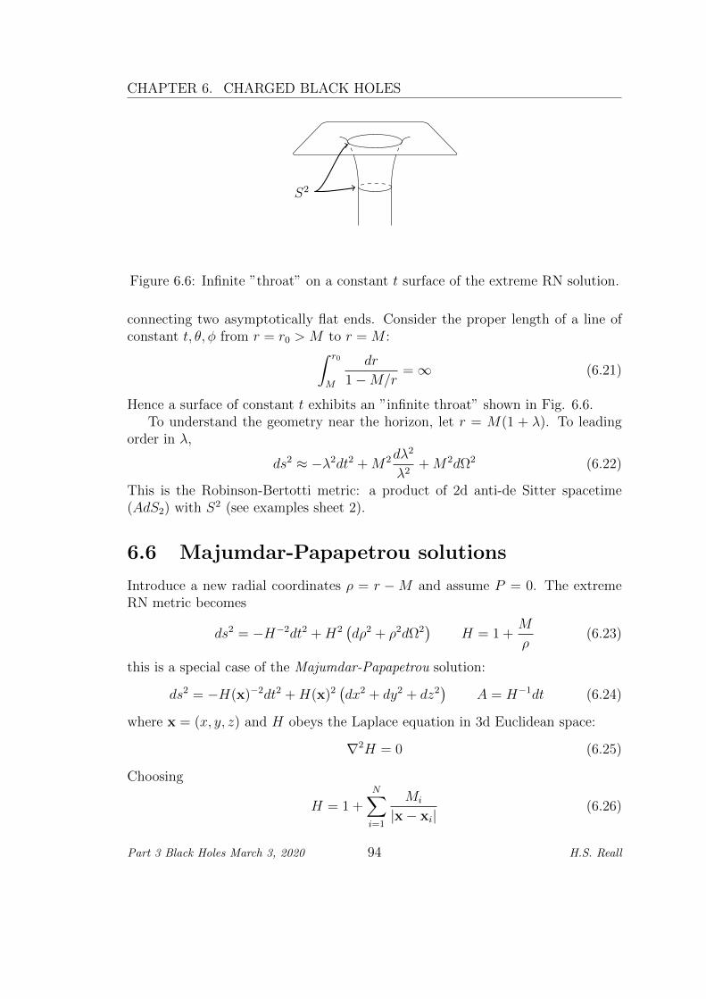
CHAPTER 6. CHARGED BLACK HOLES
S2
Figure 6.6: Infinite ”throat” on a constant t surface of the extreme RN solution.
connecting two asymptotically flat ends. Consider the proper length of a line ofconstant t, θ, φ from r = r0 > M to r = M :∫ r0
M
dr
1−M/r=∞ (6.21)
Hence a surface of constant t exhibits an ”infinite throat” shown in Fig. 6.6.To understand the geometry near the horizon, let r = M(1 + λ). To leading
order in λ,
ds2 ≈ −λ2dt2 +M2dλ2
λ2+M2dΩ2 (6.22)
This is the Robinson-Bertotti metric: a product of 2d anti-de Sitter spacetime(AdS2) with S2 (see examples sheet 2).
6.6 Majumdar-Papapetrou solutions
Introduce a new radial coordinates ρ = r −M and assume P = 0. The extremeRN metric becomes
ds2 = −H−2dt2 +H2(dρ2 + ρ2dΩ2
)H = 1 +
M
ρ(6.23)
this is a special case of the Majumdar-Papapetrou solution:
ds2 = −H(x)−2dt2 +H(x)2(dx2 + dy2 + dz2
)A = H−1dt (6.24)
where x = (x, y, z) and H obeys the Laplace equation in 3d Euclidean space:
∇2H = 0 (6.25)
Choosing
H = 1 +N∑i=1
Mi
|x− xi|(6.26)
Part 3 Black Holes March 3, 2020 94 H.S. Reall

6.6. MAJUMDAR-PAPAPETROU SOLUTIONS
gives a static solution describing N extreme RN black holes of masses Mi at po-sitions xi (each of these is an S2, not a point). Physically, such a solution existsbecause Mi = Qi for all i hence there is an exact cancellation of gravitationalattraction and electromagnetic repulsion between the black holes.
Part 3 Black Holes March 3, 2020 95 H.S. Reall

CHAPTER 6. CHARGED BLACK HOLES
Part 3 Black Holes March 3, 2020 96 H.S. Reall

Chapter 7
Rotating black holes
In this chapter we will discuss the Kerr solution, which describes a stationary rotat-ing black hole. The solution is considerably more complicated than the sphericallysymmetric solutions that we have discussed so far. We will start by explainingwhy the Kerr solution is believed to be the unique stationary black hole solution.
7.1 Uniqueness theorems
Black holes form by gravitational collapse, a time-dependent process. However, wewould expect an isolated black hole eventually to settle down to a time-independentequilibrium state (this is actually a very fast process, occuring on a time scale setby the radius of the black hole: microseconds for a solar mass black hole). Henceit is desirable to classify all such equilibrium states, i.e., all possible stationaryblack hole solutions of the vacuum Einstein (or Einstein-Maxwell) equations.
First we will need to weaken slightly our definition of ”stationary” to coverrotating black holes:
Definition. A spacetime asymptotically flat at null infinity is stationary if itadmits a Killing vector field ka that is timelike in a neighbourhood of I±. It isstatic if it is stationary and ka is hypersurface-orthogonal.
It is conventional to normalize ka so that k2 → −1 at I±. Sometimes the term”strictly stationary/static” is used if ka is timelike everywhere, not just near I±.So Minkowski spacetime is strictly static. The Kruskal spacetime is static but notstrictly static (because ka is spacelike in regions II, III).
So far, we have discussed only spherically symmetric black holes. But rotatingblack holes cannot be spherically symmetric. However, they can be axisymmetric,i.e. ”symmetric under rotations about an axis”. For a stationary spacetime wedefine this as follows.
97

CHAPTER 7. ROTATING BLACK HOLES
Definition. A spaetime asymptotically flat at null infinity is stationary and ax-isymmetric if (i) it is stationary; (ii) it admits a Killing vector field ma that isspacelike near I±; (iii) ma generates a 1-parameter group of isometries isomorphicto U(1); (iv) [k,m] = 0.
(We can also define the notion of axisymmetry in a non-stationary spacetimeby deleting (i) and (iv).) For such a spacetime, one can choose coordinates so thatk = ∂/∂t and m = ∂/∂φ with φ ∼ φ+ 2π.
Now recall that a spherically symmetric vacuum spacetime must be static, byBirkhoff’s theorem. The converse of this is untrue: a static vacuum spacetime neednot be spherically symmetric e.g. consider the spacetime outside a cube-shapedobject. However, if the only object in the spacetime is a black hole then we have:
Theorem (Israel 1967, Bunting & Masood 1987). If (M, g) is a static,asymptotically flat, vacuum black hole spacetime that is suitably regular on, andoutside an event horizon, then (M, g) is isometric to the Schwarzschild solution.
We will not attempt to describe precisely what ”suitably regular” means here.This theorem establishes that static vacuum multi black hole solutions do notexist. There is an Einstein-Maxwell generalisation of this theorem, which statesthat such a solution is either Reissner-Nordstrom or Majumdar-Papapetrou.
For stationary black holes, we have the following:
Theorem (Hawking 1973, Wald 1992). If (M, g) is a stationary, non-static,asymptotically flat analytic solution of the Einstein-Maxwell equations that issuitably regular on, and outside an event horizon, then (M, g) is stationary andaxisymmetric.
This is sometimes stated as ”stationary implies axisymmetric” for black holes.But this theorem has the unsatisfactory assumption that the spacetime be analytic.This is unphysical: analyticity implies that the full spacetime is determined by itsbehaviour in the neighbourhood of a single point. If one accepts the above result,or simply assumes axisymmetry, then
Theorem (Carter 1971, Robinson 1975). If (M, g) is a stationary, axisym-metric, asymptotically flat vacuum spacetime suitably regular on, and outside, aconnected event horizon then (M, g) is a member of the 2-parameter Kerr (1963)family of solutions. The parameters are mass M and angular momentum J .
These results lead to the expectation that the final state of gravitational col-lapse is generically a Kerr black hole. This implies that the final state is fullycharacterized by just 2 numbers: M and J . In contrast, the initial state can bearbitrarily complicated. Nearly all information about the initial state is lost duringgravitational collapse (either by radiation to infinity, or by falling into the black
Part 3 Black Holes March 3, 2020 98 H.S. Reall

7.2. THE KERR-NEWMAN SOLUTION
hole), with just the 2 numbers M,J required to describe the final state on, andoutside, the event horizon.
There is an Einstein-Maxwell generalization of the above theorem, which statesthat (M, g) should belong to the 4-parameter Kerr-Newman (1965) solution de-scribed in the next section.
7.2 The Kerr-Newman solution
This is a rotating, charged solution of Einstein-Maxwell theory. In Boyer-Lindquistcoordinates, it is
ds2 = −(∆− a2 sin2 θ
)Σ
dt2 − 2a sin2 θ(r2 + a2 −∆)
Σdtdφ
+
((r2 + a2)2 −∆a2 sin2 θ
Σ
)sin2 θdφ2 +
Σ
∆dr2 + Σdθ2
A = −Qr(dt− a sin2 θdφ) + P cos θ (adt− (r2 + a2)dφ)
Σ(7.1)
where
Σ = r2 + a2 cos2 θ ∆ = r2 − 2Mr + a2 + e2 e =√Q2 + P 2 (7.2)
At large r, the coordinates (t, r, θ, φ) reduce to spherical polar coordinates inMinkowski spacetime. In particular, (θ, φ) have their usual interpretation as angleson S2 so 0 < θ < π and φ ∼ φ + 2π. It can be shown that the KN solution isasymptotically flat at null infinity.
The solution is stationary and axisymmetric with two commuting Killing vectorfields:
ka =
(∂
∂t
)ama =
(∂
∂φ
)a(7.3)
ka is timelike near infinity although, as we will discuss, it is not globally timelike.The solution possesses a discrete isometry t→ −t, φ→ −φ which simultaneouslyreverses the direction of time and the sense of rotation.
The solution has 4 parameters: M,a,Q, P . We’ll see later that M is the mass,Q the electric charge, P the magnetic charge and a = J/M where J is the angularmomentum. When a = 0 the KN solution reduces to the RN solution. Note thatφ→ −φ has the same effect as a→ −a so there is no loss of generality in assuminga ≥ 0.
Part 3 Black Holes March 3, 2020 99 H.S. Reall
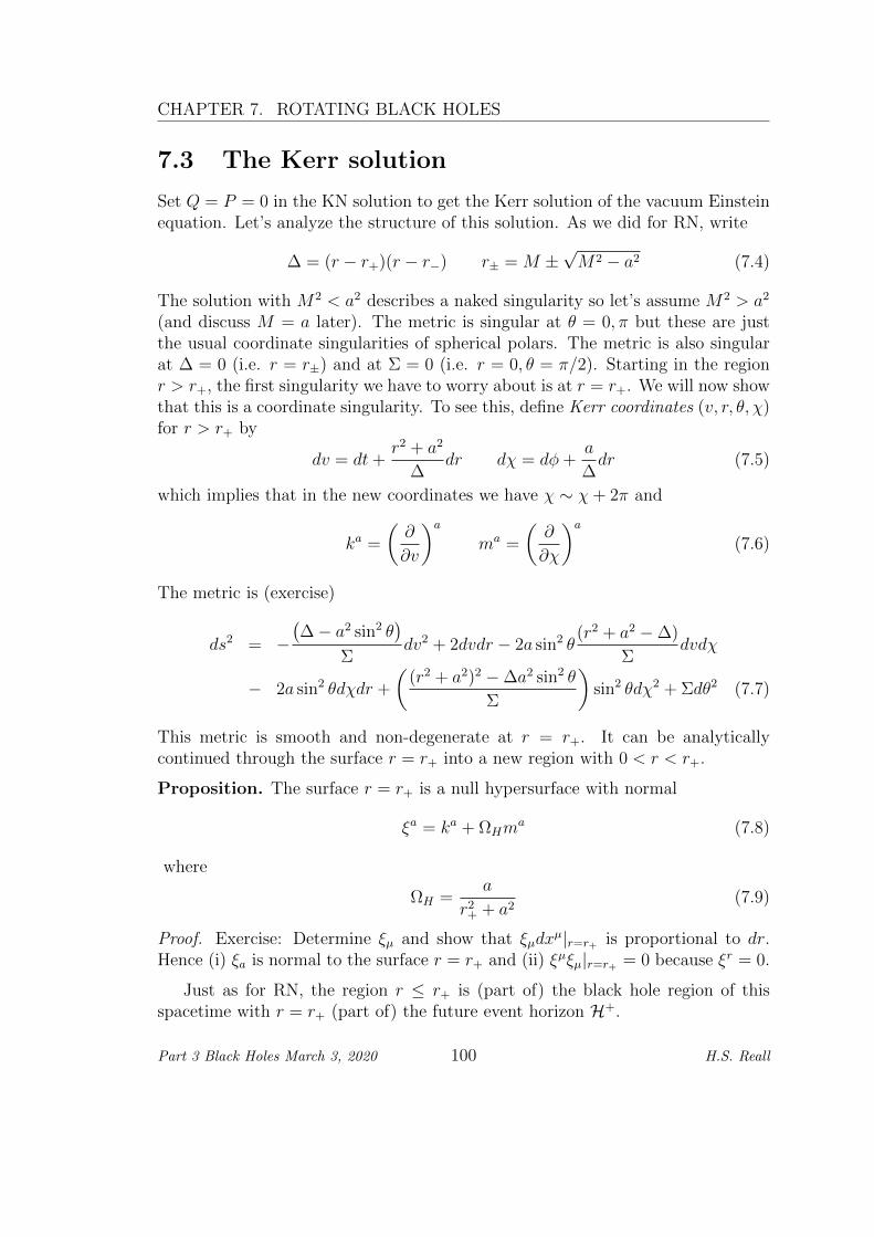
CHAPTER 7. ROTATING BLACK HOLES
7.3 The Kerr solution
Set Q = P = 0 in the KN solution to get the Kerr solution of the vacuum Einsteinequation. Let’s analyze the structure of this solution. As we did for RN, write
∆ = (r − r+)(r − r−) r± = M ±√M2 − a2 (7.4)
The solution with M2 < a2 describes a naked singularity so let’s assume M2 > a2
(and discuss M = a later). The metric is singular at θ = 0, π but these are justthe usual coordinate singularities of spherical polars. The metric is also singularat ∆ = 0 (i.e. r = r±) and at Σ = 0 (i.e. r = 0, θ = π/2). Starting in the regionr > r+, the first singularity we have to worry about is at r = r+. We will now showthat this is a coordinate singularity. To see this, define Kerr coordinates (v, r, θ, χ)for r > r+ by
dv = dt+r2 + a2
∆dr dχ = dφ+
a
∆dr (7.5)
which implies that in the new coordinates we have χ ∼ χ+ 2π and
ka =
(∂
∂v
)ama =
(∂
∂χ
)a(7.6)
The metric is (exercise)
ds2 = −(∆− a2 sin2 θ
)Σ
dv2 + 2dvdr − 2a sin2 θ(r2 + a2 −∆)
Σdvdχ
− 2a sin2 θdχdr +
((r2 + a2)2 −∆a2 sin2 θ
Σ
)sin2 θdχ2 + Σdθ2 (7.7)
This metric is smooth and non-degenerate at r = r+. It can be analyticallycontinued through the surface r = r+ into a new region with 0 < r < r+.
Proposition. The surface r = r+ is a null hypersurface with normal
ξa = ka + ΩHma (7.8)
where
ΩH =a
r2+ + a2
(7.9)
Proof. Exercise: Determine ξµ and show that ξµdxµ|r=r+ is proportional to dr.
Hence (i) ξa is normal to the surface r = r+ and (ii) ξµξµ|r=r+ = 0 because ξr = 0.
Just as for RN, the region r ≤ r+ is (part of) the black hole region of thisspacetime with r = r+ (part of) the future event horizon H+.
Part 3 Black Holes March 3, 2020 100 H.S. Reall

7.4. MAXIMAL ANALYTIC EXTENSION
In BL coordinates we have ξ = ∂/∂t+ ΩH∂/∂φ. Hence ξµ∂µ (φ− ΩHt) = 0 soφ = ΩHt+ const. on orbits (integral curves) of ξa. Note that φ = const. on orbitsof ka. Hence particles moving on orbits of ξa rotate with angular velocity ΩH withrespect to a stationary observer (i.e. someone on an orbit of ka). In particular,they rotate with this angular velocity w.r.t. a stationary observer at infinity. Sinceξa is tangent to the generators of H+, it follows that these generators rotate withangular velocity ΩH w.r.t. a stationary observer at infinity, so we interpret ΩH asthe angular velocity of the black hole.
7.4 Maximal analytic extension
The Kerr coordinates are analogous to the ingoing EF coordinates we used for RN.One can similarly define coordinates analogous to retarded EF coordinates and usethese to construct an analytic extension into a white hole region. Then, just as forRN, one can define Kruskal-like coordinates that cover all of these regions, as wellas a new asymptotically flat region, i.e., there are regions analogous to regions Ito IV of the analytically extended RN solution.
Just as for RN, the spacetime can be analytically extended across null hyper-surfaces at r = r− in regions II and III. The resulting maximal analytic extensionis similar to that of RN except for the behaviour near the singularity. In the Kerrcase, it turns out that the curvature singularity has the structure of a ring and bypassing through the ring one can enter a new asymptotically flat region. One alsofinds that ma becomes timelike near the singularity. The orbits of ma are closed(because φ ∼ φ+ 2π) hence there are closed timelike curves near the singularity.
The Kerr solution is not spherically symmetric so one can’t draw a Penrosediagram for it. However, if one considers the submanifold of the spacetime corre-sponding to the axis of symmetry (θ = 0 or θ = π) then, since this submanifoldis two-dimensional, one can draw a Penrose diagram for it. Note that this sub-manifold is ”totally geodesic”, i.e., a geodesic initially tangent to it will remaintangent. (The same is true for the ”equatorial plane” θ = π/2.) The resultingdiagram takes the following form shown in Fig. 7.1.
Most of this diagram is unphysical because, just as for RN, the null hypersur-faces r = r− are Cauchy horizons for a geodesically complete, asymptotically flat(with 2 ends) surface Σ. Hence the spacetime beyond r = r− is not determineduniquely by the data on Σ (unless one makes the unphysical assumption of ana-lyticity). By the same argument as for RN, these Cauchy horizons are expectedto be unstable against small perturbations in region I (or IV), with the perturbedspacetime exhibiting null or spacelike singularities instead of Cauchy horizons, inagreement with strong cosmic censorship.
When we studied the Schwarzschild solution, we saw that it describes the
Part 3 Black Holes March 3, 2020 101 H.S. Reall
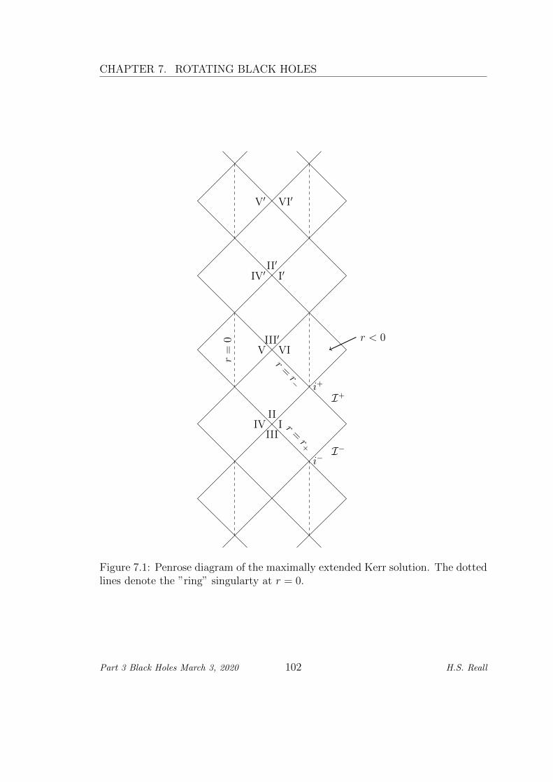
CHAPTER 7. ROTATING BLACK HOLES
VI′V′
I′II′
IV′
VIIII′
V
III
IIIIV r
=r+
r=r−
r=
0
I+
I−
i+
i−
r < 0
Figure 7.1: Penrose diagram of the maximally extended Kerr solution. The dottedlines denote the ”ring” singularty at r = 0.
Part 3 Black Holes March 3, 2020 102 H.S. Reall

7.5. THE ERGOSPHERE AND PENROSE PROCESS
metric outside a spherical star. This was a consequence of Birkhoff’s theorem. Incontrast, the Kerr solution does not describe the spacetime outside a rotating star.This solution is expected to describe only the ”final state” of gravitational collapse.One can’t obtain a solution describing gravitational collapse to form a Kerr blackhole simply by ”gluing in” a ball of collapsing matter as we did for Schwarzschild.In particular, the spacetime during such collapse would be non-stationary becausethe collapse would lead to emission of gravitational waves.
Finally, the special case M = a is called the extreme Kerr solution. It is a blackhole solution with several properties similar to those of the extreme RN solution.In particular, surfaces of constant t exhibit an ”infinite throat” andH± are Cauchyhorizons for surfaces of constant t.
7.5 The ergosphere and Penrose process
In BL coordinates, consider the norm of the Killing vector field ka:
k2 = gtt = −(∆− a2 sin2 θ
)Σ
= −(
1− 2Mr
r2 + a2 cos2 θ
)(7.10)
Hence ka is timelike in region I if and only if r2 − 2Mr + a2 cos2 θ > 0 i.e. if, andonly if r > M +
√M2 − a2 cos2 θ. Hence ka is spacelike in the following region
outside H+
r+ = M +√M2 − a2 < r < M +
√M2 − a2 cos2 θ (7.11)
This region is called the ergosphere. Its surface is called the ergosurface. Thelatter intersects H+ at the poles θ = 0, π, as shown in Fig. 7.2.
A stationary observer is someone with 4-velocity parallel to ka. Such observersdo not exist in the ergosphere because ka is spacelike there. Any causal curve inthe ergosphere must rotate (relative to observers at infinity) in the same directionas the black hole.
Consider a particle with 4-momentum P a = µua (where µ is rest mass and ua
is 4-velocity). Let the particle approach a Kerr black hole along a geodesic. Theenergy of the particle according to a stationary observer at infinity is the conservedquantity along the geodesic
E = −k · P (7.12)
Suppose that the particle decays at a point p inside the ergosphere into two otherparticles with 4-momenta P a
1 and P a2 (Fig. 7.3). From the equivalence principle,
we know that the decay must conserve 4-momentum (because we can use specialrelativity in a local inertial frame at p) hence
P a = P a1 + P a
2 ⇒ E = E1 + E2 (7.13)
Part 3 Black Holes March 3, 2020 103 H.S. Reall

CHAPTER 7. ROTATING BLACK HOLES
θ = 0
θ = π
ergosurfaceergosphere
Figure 7.2: Ergosphere of a Kerr black hole.
P
P1
P2
Figure 7.3: Decay of a particle inside the ergosphere.
where Ei = −k · Pi. Since ka is spacelike within the ergoregion, it is possible thatE1 < 0. We must then have E2 = E + |E1| > E. It can be shown that the firstparticle must fall into the black hole and the second one can escape to infinity.This particle emerges from the ergoregion with greater energy than the particlethat was sent in! Energy is conserved because the particle that falls into the blackhole carries in negative energy, so the energy (mass) of the black hole decreases.This Penrose process is a method for extracting energy from a rotating black hole.
How much energy can be extracted in this process? A particle crossing H+
must have −P · ξ ≥ 0 because both P a and ξa are future-directed causal vectors.But ξa = ka + ΩHm
a hence
E − ΩHL ≥ 0 (7.14)
Part 3 Black Holes March 3, 2020 104 H.S. Reall

7.5. THE ERGOSPHERE AND PENROSE PROCESS
where E is the energy of the particle and
L = m · P (7.15)
is its conserved angular momentum. Hence we have L ≤ E/ΩH (recall our con-vention a > 0 so ΩH > 0). The particle carries energy E and angular momentumL into the black hole. If the black hole now settles down to a Kerr solution thenthis new Kerr solution will have slightly different mass and angular momentum:δM = E and δJ = L. Therefore
δJ ≤ δM
ΩH
=2M(M2 +
√M4 − J2)
JδM (7.16)
Exercise. Show that this is equivalent to δMirr ≥ 0 where the irreducible mass is
Mirr =
[1
2
(M2 +
√M4 − J2
)]1/2
(7.17)
Inverting this expression gives
M2 = M2irr +
J2
4M2irr
≥M2irr (7.18)
Hence in the Penrose process it is not possible to reduce the mass of the black holebelow the initial value of Mirr: there is a limit to the amount of energy that canbe extracted.
Exercise. Show that A = 16πM2irr is the ”area of the event horizon” of a Kerr
black hole, i.e., the area of the intersection of H+ with a partial Cauchy surface(e.g. a surface v = const in Kerr coordinates).
Hence δA ≥ 0 in the Penrose process: the area of the event horizon is non-decreasing. This is a special case of the second law of black hole mechanics. Theexplicit expression for A is
A = 8π(M2 +
√M4 − J2
)(7.19)
Part 3 Black Holes March 3, 2020 105 H.S. Reall

CHAPTER 7. ROTATING BLACK HOLES
Part 3 Black Holes March 3, 2020 106 H.S. Reall

Chapter 8
Mass, charge and angularmomentum
8.1 Charges in curved spacetime
On an orientable n-dimensional manifold with a metric, we denote the volumeform by εa1...an . This can be shown to obey
εa1...apcp+1...cnεb1...bpcp+1...cn = ±p!(n− p)!δa1[b1. . . δ
apbp] (8.1)
where the upper (lower) sign holds for Riemannian (Lorentzian) signature.
Definition. The Hodge dual of a p-form X is the (n− p)-form ? X defined by
(? X)a1...an−p =1
p!εa1...an−pb1...bpX
b1...bp (8.2)
Lemma. For a p-form X
?(? X) = ±(−1)p(n−p)X (8.3)
(? d ? X)a1...ap−1 = ±(−1)p(n−p)∇bXa1...ap−1b (8.4)
where the upper (lower) sign holds for Riemannian (Lorentzian) signature.
Proof. Use (8.1).For example, in 3d Euclidean space, the usual operations of vector calculus can
be written using differential forms as
∇f = df div X = ? d ? X curl X = ? dX (8.5)
where f is a function and X denotes the 1-form Xa obtained from a vector fieldXa. The final equation shows that the exterior derivative can be thought of as ageneralization of the curl operator.
107

CHAPTER 8. MASS, CHARGE AND ANGULAR MOMENTUM
Another example is Maxwell’s equations
∇aFab = −4πjb ∇[aFbc] = 0 (8.6)
where ja is the current density vector. These can be written as
d ? F = −4π ? j, dF = 0 (8.7)
The first of these implies d ? j = 0, which is equivalent to ∇aja = 0, i.e., ja is
a conserved current. The second of these implies (by the Poincare lemma) thatlocally there exists a 1-form A such that F = dA.
Now consider a spacelike hypersurface Σ. We define the total electric chargeon Σ to be
Q = −∫
Σ
?j (8.8)
(The orientation of Σ is fixed by regarding Σ as a boundary of J−(Σ) and choosingthe orientation used in Stokes’ theorem.) Using Maxwell’s equations we can write
Q =1
4π
∫Σ
d ? F (8.9)
Hence if Σ is a manifold with boundary ∂Σ then Stokes’ theorem gives
Q =1
4π
∫∂Σ
?F (8.10)
This expresses the total charge on Σ in terms of an integral of ?F over ∂Σ. It isthe curved space generalisation of Gauss’ law Q ∼
∫E · dS.
For example, consider Minkowski spacetime in spherical polar coordinates,choosing the orientation so that the volume form is r2 sin θdt ∧ dr ∧ dθ ∧ dφ. LetΣ be the surface t = 0. If we regard this as the boundary of the region t ≤ 0then Stokes’ theorem fixes the orientation of Σ as dr∧ dθ∧ dφ. Now let ΣR be theregion r ≤ R of Σ, whose boundary is S2
R: the sphere t = 0, r = R. Stokes tellsus to pick the orientation of S2
R to be dθ ∧ dφ. Consider a Coulomb potential
A = −qrdt ⇒ F = − q
r2dt ∧ dr (8.11)
Taking the Hodge dual gives
(?F )θφ = r2 sin θF tr = q sin θ (8.12)
and hence the charge on ΣR is
Q[ΣR] =1
4π
∫S2R
?F =1
4π
∫dθdφ q sin θ = q (8.13)
Part 3 Black Holes March 3, 2020 108 H.S. Reall

8.2. KOMAR INTEGRALS
so our definition of Q indeed gives the correct result.For an asymptotically flat hypersurface in Minkowski spacetime we can take the
limit R→∞ to express the total charge on Σ as an integral at infinity. Motivatedby this, we now define the total charge for any asymptotically flat end:
Definition. Let (Σ, hab, Kab) be an asymptotically flat end. Then the electric andmagnetic charges associated to this end are
Q =1
4πlimr→∞
∫S2r
?F P =1
4πlimr→∞
∫S2r
F (8.14)
where S2r is a sphere xixi = r2 where xi are the coordinates used in the definition
of an asymptotically flat end.
Exercise (examples sheet 3). Show that these definitions agree with Q,P usedin the Kerr-Newman solution.
Hence the charges can be non-zero even when no charged matter is present inthe spacetime (i.e. ja = 0). Consider a surface of constant t in Kerr-Newman(or Reissner-Nordstrom). The total charge on this surface is zero. But when weconvert it to a surface integral at infinity, we get two terms because the surfacehas two asymptotically flat ends. Hence the charges of these two ends must beequal in magnitude with opposite sign.
8.2 Komar integrals
If (M, g) is stationary then there exists a conserved energy-momentum current
Ja = −Tabkb d ? J = 0 (8.15)
Hence one can define the total energy of matter on a spacelike hypersurface Σ as
E[Σ] = −∫
Σ
?J (8.16)
This is conserved: if Σ,Σ′ bound a spacetime region R (Fig. 8.1) then
E[Σ′]− E[Σ] = −∫∂R
?J = −∫R
d ? J = 0 (8.17)
Note that we need not require that the energy-momentum tensor Tab usedabove is the one appearing on the RHS of the Einstein equation. It could be thetime-dependent energy momentum tensor of a test field in a stationary vacuumspacetime.
Part 3 Black Holes March 3, 2020 109 H.S. Reall

CHAPTER 8. MASS, CHARGE AND ANGULAR MOMENTUM
Σ′
Σ
R
Figure 8.1: Region R bounded by Σ,Σ′.
Now if we had ?J = dX for some 2-form X then we could convert E[Σ] to anintegral over ∂Σ as we did in the previous section. We could then define the totalenergy for a general asymptotically flat end. Unfortunately, this is not possible.However, consider
(?d ? dk)a = −∇b(dk)ab = −∇b∇akb +∇b∇bka = 2∇b∇bka (8.18)
where we using Killing’s equation. Now recall
Lemma. A Killing vector field ka obeys
∇a∇bkc = Rc
badkd (8.19)
Hence we have
(?d ? dk)a = −2Rabkb = 8πJ ′a (8.20)
where we used Einstein’s equation (so henceforth Tab must be the one appearingEinstein’s equation) and
J ′a = −2
(Tab −
1
2Tgab
)kb (8.21)
Therefored ? dk = 8π ? J ′ (8.22)
So ?J ′ is exact (and conserved: d ? J ′ = 0). It follows that
−∫
Σ
?J ′ = − 1
8π
∫Σ
d ? dk = − 1
8π
∫∂Σ
?dk (8.23)
The LHS appears to be a measure of the energy-momentum content of space-time.
Exercise. Consider a static, spherically symmetric, perfect fluid star. Let Σ bethe region r ≤ r0 of a surface of constant t where r0 > R. Show that the RHSof (8.23) is the Schwarzschild parameter M . Show that, in the Newtonian limit,(p ρ, |Φ| 1, |Ψ| 1), the LHS of (8.23) is the total mass of the fluid.
Part 3 Black Holes March 3, 2020 110 H.S. Reall

8.3. HAMILTONIAN FORMULATION OF GR
Hence M is the mass of the star in the Newtonian limit. This motivates thefollowing definition:
Definition. Let (Σ, hab, Kab) be an asymptotically flat end in a stationary space-time. The Komar mass (or Komar energy) is
MKomar = − 1
8πlimr→∞
∫S2r
?dk (8.24)
with S2r defined as above.
The Komar mass is a measure of the total energy of the spacetime. This energycomes both from matter and from the gravitational field. For example, the firstpart of the above exercise shows that the Komar mass of a Schwarzschild blackhole is non-zero, even when no matter is present in the spacetime.
The only property of ka that we used above is the Killing property. In anaxisymmetric spacetime we have a Killing vector field ma that generates rotationsabout the axis of symmetry. Using this we can define the angular momentum ofan axisymmetric spacetime:
Definition. Let (Σ, hab, Kab) be an asymptotically flat end in an axisymmetricspacetime. The Komar angular momentum is
JKomar =1
16πlimr→∞
∫S2r
?dm (8.25)
Exercise (examples sheet 3). Show that MKomar = M and JKomar = J for theKerr-Newman solution.
8.3 Hamiltonian formulation of GR
The Komar mass can be defined only in a stationary spacetime. How do wedefine energy in a non-stationary spacetime? Energy is defined as the value ofthe Hamiltonian. So we need to consider the Hamiltonian formulation of GR. Forsimplicity we’ll work in vacuum, i.e., no matter fields present. It is also convenientto change our units. Previously we have set G = 1. But in this section we will set16πG = 1 instead.
Recall that in the 3 + 1 decomposition of spacetime, we consider a spacetimefoliated with surfaces of constant t, so that the metric takes the form
ds2 = −N2dt2 + hij(dxi +N idt)(dxj +N jdt) (8.26)
Part 3 Black Holes March 3, 2020 111 H.S. Reall

CHAPTER 8. MASS, CHARGE AND ANGULAR MOMENTUM
where N is the lapse function and N i the shift vector. If one substitutes this intothe Einstein-Hilbert action then the resulting action is, neglecting surface terms,
S =
∫dtd3xL =
∫dtd3x
√hN
((3)R +KijK
ij −K2)
(8.27)
where (3)R is the Ricci scalar of hij, Kij is the extrinsic curvature of a surface ofconstant t, with trace K, and ij indices on the RHS are raised with hij, the inverseof hij. The extrinsic curvature can be written
Kij =1
2N
(hij −DiNj −DjNi
)(8.28)
where a dot denotes a t-derivative and Di is the covariant derivative associated tohij on a surface of constant t.
The action S is a functional of N , N i and hij. Note that it does not dependon time derivatives of N or N i. Varying N gives the hamiltonian constraint fora surface of constant t. Similarly, varying N i gives the momentum constraint.Varying hij gives the evolution equation for hij. There are no evolution equationsfor N,N i: these functions are not dynamical but can be freely specified, whichamounts to a choice of coordinates.
To introduce the Hamiltonian formulation of GR, we need to determine themomenta conjugate to N , N i and hij. Since the action does not depend on timederivatives of N and N i, it follows that their conjugate momenta are identicallyzero. The momentum conjugate to hij is
πij ≡ δS
δhij=√h(Kij −Khij
)(8.29)
Note that the factor of√h means that πij is not a tensor, it is an example of
a tensor density. (A tensor density of weight p transforms under a coordinatetransformation in the same way as hp times a tensor.)
Now we define the Hamiltonian as the Legendre transform of the Lagrangian:
H =
∫d3x
(πijhij − L
)(8.30)
If we integrate by parts and neglect surface terms, this gives
H =
∫d3x√h(NH +N iHi
)(8.31)
where
H = −(3)R + h−1πijπij −1
2h−1π2 (8.32)
Part 3 Black Holes March 3, 2020 112 H.S. Reall

8.3. HAMILTONIAN FORMULATION OF GR
Hi = −2hikDj
(h−1/2πjk
)(8.33)
with π ≡ hijπij. In the Hamiltonian formalism, hij and πij are the dynami-cal variables. N and N i play the role of Lagrange multipliers, i.e., we demandδH/δN = δH/δN i = 0, which gives H = Hi = 0. These are simply the Hamilto-nian and momentum constraints. The equations of motion are given by Hamilton’sequations:
hij =δH
δπijπij = − δH
δhij(8.34)
The first of these just reproduces the definition of πij. The second equation isquite lengthy.
Now we’ve determined the Hamiltonian for GR, we can define the energy of asolution as the value of the Hamiltonian. But (8.31) vanishes for any solution ofthe constraint equations!
The resolution of this puzzle is that we need to add a boundary term to theHamiltonian. To calculate the variational derivatives in (8.34) we need to integrateby parts in order to remove derivatives from δπij and δhij. This generates surfaceterms. We need to investigate whether neglecting these terms is legitimate. Ifthe constant t surfaces are compact then there won’t be any surface terms. So inthis case, referred to as a closed universe, the Hamiltonian really does evaluate tozero on a solution. This remains true when matter is included. Hence, in GR, thetotal energy of a closed universe is exactly zero. (This leads to speculation aboutquantum creation of a closed universe from nothing...)
Now consider the case in which the surfaces constant t are not spatially com-pact. Let’s assume that each of these surfaces is asymptotically flat with 1 end.Hence we can introduce ”almost Cartesian” coordinates so that as r →∞ we havehij = δij + O(1/r) and πij = O(1/r2). Hence the natural boundary conditionson the variations of hij and πij are δhij = O(1/r) and δπij = O(1/r2). We alsoassume our time foliation is chosen so that t, xi approach ”inertial” coordinates inMinkowski spacetime at large r. More precisely, assume that N = 1 +O(1/r) andN i → 0 as r →∞.
Consider the region of our constant t surface contained within a sphere ofconstant r, with boundary S2
r . When we vary πij, the resulting surface term onS2r is ∫
S2r
dA(−2N ihiknjh
−1/2δπjk)
(8.35)
where dA is the area element, and nj the outward unit normal, of S2r . Now
dA = O(r2) but our boundary conditions imply that the expression in bracketsdecays faster than 1/r2 as r →∞ hence the whole expression vanishes as r →∞.So we don’t need to worry about the surface term that arises when we vary πij.
Part 3 Black Holes March 3, 2020 113 H.S. Reall

CHAPTER 8. MASS, CHARGE AND ANGULAR MOMENTUM
When we vary hij, surface terms arise in two ways. First, the variation of h−1/2
in Hi is within a derivative so we need to integrate by parts, generating a surfaceterm. This is very similar to the surface term above and vanishes as r → ∞.Second, we have the variation of the term (3)R in H. You know the variation ofthe Ricci scalar because this is what you need to calculate when you derive theEinstein equation from the Einstein-Hilbert action. The only difference is that weare now varying a 3d, rather than a 4d, Ricci scalar:
δ(3)R = −Rijδhij +DiDjδhij −DkDk
(hijδhij
)(8.36)
When we calculate δH, we need to integrate by parts twice to eliminate thesederivatives on δhij. The first integration by parts gives the surface term
S1 = −∫S2r
dA N[niDjδhij − nkDk(h
ijδhij)]
(8.37)
and the second integration by parts gives another surface term
S2 =
∫S2r
dA(njδhijD
iN − hijδhijnkDkN)
(8.38)
Our boundary conditions implies that S2 → 0 as r → ∞. On the other hand, wehave
limr→∞
S1 = − limr→∞
∫S2r
dA ni (∂jδhij − ∂iδhjj) (8.39)
Here we have used the fact that hij → δij so (a) Dk → ∂k as r → ∞ and (b) wedon’t need to distinguish between ”upstairs” and ”downstairs” indices. But wecan rewrite this as
limr→∞
S1 = −δEADM (8.40)
where
EADM = limr→∞
∫S2r
dA ni (∂jhij − ∂ihjj) (8.41)
In general, δEADM will be non-zero. But now consider
H ′ = H + EADM (8.42)
Since H ′ and H differ by a surface term, they will give the same equations ofmotion. However, when we vary hij in H ′, the boundary term S1 coming from thevariation of H will be cancelled by the variation of the surface term EADM . Henceno surface terms arise in the variation of H ′ so H ′ must be the Hamiltonian forGeneral Relativity with asymptotically flat initial data. The need for this surfaceterm was first pointed out by Regge and Teitelboim (1974).
Part 3 Black Holes March 3, 2020 114 H.S. Reall
8.4. ADM ENERGY
8.4 ADM energy
Now that we have a satisfactory variational principle, we can evaluate the Hamil-tonian on a solution. As before, we have that H = 0 so the value of H ′ is the valueof the surface term EADM . Hence EADM must be the energy of our initial dataset. This is the Arnowitt-Deser-Misner energy (1962). We now return to G = 1units to obtain the following
Definition. The ADM energy of an asymptotically flat end is
EADM =1
16πlimr→∞
∫S2r
dA ni (∂jhij − ∂ihjj) (8.43)
If we have asymptotically flat initial data with several asymptotically flat endsthen one can define a separate ADM energy for each asymptotic end. In a station-ary, asymptotically flat spacetime, it can be shown that EADM = MKomar if onechooses the surfaces of constant t to be orthogonal to the timelike Killing vectorfield as r →∞.
Exercise (examples sheet 3). Show that EADM = M for a constant t surfacein the Kerr-Newman solution.
There is also a notion of the total 3-momentum of an asymptotically flat end:
Definition. The ADM 3-momentum of an asymptotically flat end is
Pi =1
8πlimr→∞
∫S2r
dA (Kijnj −Kni) (8.44)
In Newtonian gravity, the energy density of the gravitational field is negative.
So one might wonder whether the ADM energy in GR could also be negative.Since EADM = M for a surface of constant t in the Schwarzschild spacetime, itfollows that EADM < 0 for M < 0 Schwarzschild. But in this case, the surfaceof constant t is singular (not geodesically complete). We could also arrange thatEADM < 0 if we included matter with negative energy density. But if we excludethese unphysical possibilities then we have the positive energy theorem:
Theorem (Schoen & Yau 1979, Witten 1981). Let (Σ, hab, Kab) be an initialdata set that is geodesically complete and asymptotically flat. Assume that theenergy-momentum tensor satisfies the dominant energy condition. Then EADM ≥√PiPi, with equality if, and only if, (Σ, hab, Kab) arises from a surface in Minkowski
spacetime.
In the case of a spacetime containing black holes, one might not want to assumeanything about the black hole interior. In this case, one can allow Σ to have an
Part 3 Black Holes March 3, 2020 115 H.S. Reall
CHAPTER 8. MASS, CHARGE AND ANGULAR MOMENTUM
inner boundary corresponding to an apparent horizon and the result still holds(Gibbons, Hawking, Horowitz & Perry 1983).
There is a natural way of regarding (EADM , Pi) as a 4-vector defined at spatialinfinity i0. We then define the ADM mass by
MADM =√E2ADM − PiPi ≥ 0 (8.45)
Part 3 Black Holes March 3, 2020 116 H.S. Reall

Chapter 9
Black hole mechanics
9.1 Killling horizons and surface gravity
Definition. A null hypersurface N is a Killing horizon if there exists a Killingvector field ξa defined in a neighbourhood of N such that ξa is normal to N .
Theorem (Hawking 1972). In a stationary, analytic, asymptotically flat vac-uum black hole spacetime, H+ is a Killing horizon.
Proof. See Hawking and Ellis.
The result extends to Einstein-Maxwell theory or theories where the matterfields obey hyperbolic equations. As mentioned previously, it would be desirableto eliminate the assumption of analyticity because analyticity implies that the fullspacetime is determined by its behaviour in a neighbourhood of a single point.
Note that H+ is not necessarily a Killing horizon of the stationary Killingvector field ka. For example, in the Kerr solution, we have ξa = ka + ΩHm
a wherema is the Killing field corresponding to axisymmetry. One can show (see Hawkingand Ellis) that this behaviour is general: if ξa is not tangent to ka then one canconstruct a linear combination ma of ξa and ka so that the spacetime is stationaryand axisymmetric.
If N is a Killing horizon w.r.t. a Killing vector field ξa then it is also a Killinghorizon w.r.t. the Killing vector field cξa where c is any non-zero constant. Ina stationary, asymptotically flat spacetime, it is conventional to normalise thegenerator of time translations so that kaka → −1 at infinity. We then normalizeξa so that so that ξa = ka + ΩHm
a.
Since ξaξa = 0 on N , it follows that the gradient of ξaξa is normal to N , i.e.,proportional to ξa. Hence there exists a function κ on N such that
∇a(ξbξb)|N = −2κξa (9.1)
117

CHAPTER 9. BLACK HOLE MECHANICS
The function κ is called the surface gravity of the Killing horizon. The LHS can berearranged to give 2ξb∇aξb = −2ξb∇bξa using Killing’s equation. Hence we have
ξb∇bξa|N = κξa (9.2)
which shows that κ measures the failure of integral curves of ξa to be affinelyparameterized. If we let na be the tangent to the affinely parameterized generatorsof N then we have ξa = fna for some function f on N . Then using n · ∇na = 0we have, on N , ξb∇bξ
a = fnanb∂bf = f−1ξaξb∂bf and hence
κ = ξa∂a log |f | (9.3)
Example. The Reissner-Nordstrom solution in ingoing EF coordinates is
ds2 = −∆
r2dv2 + 2dvdr + r2dΩ2 (9.4)
where ∆ = (r − r+)(r − r−) and r± = M ±√M2 − e2. The stationary Killing
vector field is k = ∂/∂v. At r = r± we have ∆ = 0 so ka = (dr)a, which is normalto the null hypersurfaces r = r±. Hence these surfaces are Killing horizons. Tocalculate the surface gravity we use
d(kbkb) = d(−∆/r2) = (−∆′/r2 + 2∆/r3)dr (9.5)
Evaluating at r = r± gives
d(kbkb)|r=r± = −(r± − r∓)
r2±
dr = −(r± − r∓)
r2±
k|r=r± (9.6)
hence the surface gravities are
κ = κ± =(r± − r∓)
2r2±
(9.7)
For Schwarzschild we have e = 0 so r+ = 2M , r− = 0 and hence κ = 1/4M is thesurface gravity of H+. For extreme RN we have r+ = r− and κ = 0.
Exercise. In the Kruskal spacetime, H+ is the surface U = 0 and H− the surfaceV = 0. Use (2.36) to show that these are Killing horizons of ka (the time translationKilling vector field). Calculate the LHS of (9.1). Use (2.33) to relate dr to d(UV ).Hence show that the surface gravity of H± is ±1/(4M).
Part 3 Black Holes March 3, 2020 118 H.S. Reall

9.2. INTERPRETATION OF SURFACE GRAVITY
This is an example of a bifurcate Killing horizon i.e. a pair of intersecting nullhypersurfaces N± that are each Killing horizons with respect to the same Killingvector field. At the bifurcation surface B = N+ ∩ N−, the Killing field can’t benormal to both N+ and N− so it must vanish on B. Any vector Xa tangent to Bis tangent to both N+ and N−, which implies that Xa must be spacelike so B isa spacelike surface. For the Kruskal spacetime this is the 2-sphere U = V = 0.
9.2 Interpretation of surface gravity
The main reason that κ is important is because ~κ/(2π) is the Hawking tempera-ture of the hole (see later). There is also a classical interpretation of κ.
In a static, asymptotically flat spacetime, consider a particle of unit mass that is”at rest”, i.e., following an orbit of ka. Such orbits are not geodesics so the particleis accelerating. This acceleration requires a force, let’s assume it is provided by amassless inelastic string attached to the particle, with the other end of the stringheld by an observer at infinity. Let F be the force in the string (i.e. the tension)measured at infinity. Then F → κ as we consider orbits closer and closer to aKilling horizon of ka (for the Schwarzschild solution this is proved on examplessheet 3). Hence κ is the force per unit mass required at infinity to hold a testparticle at rest near the horizon.
The local force on the particle is certainly not κ. In a general stationary space-time, the 4-velocity of a particle on an orbit of ka is
ua =ka√−k2
(9.8)
where the normalisation is fixed by the condition u2 = −1. The proper accelerationof the particle is therefore
Aa = u · ∇ua =k · ∇ka
−k2+
ka
2(−k2)2k · ∇(k2) (9.9)
In the first term, Killing’s equation gives kb∇bka = −kb∇akb = −(1/2)∂a(k2). In
the second term k · ∇(k2) = 2kakb∇akb = 0. Hence we have
Aa =∂a(−k2)
2(−k2)=
1
2∂a log(−k2) (9.10)
Since k2 → 0 at a Killing horizon, it follows that Aa must diverge at the horizon.For Schwarzschild we have (viewing Aa as a 1-form)
A =1
2d log
(1− 2M
r
)=
M
r2 (1− 2M/r)dr (9.11)
Part 3 Black Holes March 3, 2020 119 H.S. Reall

CHAPTER 9. BLACK HOLE MECHANICS
and so the norm of A is (using grr = (1− 2M/r))
|A| ≡√gabAaAb =
√M2
r4(1− 2M/r)=
M
r2√
1− 2M/r(9.12)
which diverges as r → 2M . Hence the local tension (i.e. the force exerted on theparticle by the string) is very large if the particle is near the horizon. A physicalstring would break if the particle were too near the horizon.
9.3 Zeroth law of black holes mechanics
Proposition. Consider a null geodesic congruence that contains the generatorsof a Killing horizon N . Then θ = σ = ω = 0 on N .
Proof. ω = 0 on N because the generators are hypersurface orthogonal.Let ξa be a Killing field normal to N . On N we can write ξa = hUa where Ua is
tangent to the (affinely parameterized) generators of N and h is a function on N .Let N be specified by an equation f = 0. Then we can write Ua = h−1ξa + fV a
where V a is a smooth vector field. We can then calculate
Bab = ∇bUa = (∂bh−1)ξa + h−1∇bξa + (∂bf)Va + f∇bVa (9.13)
so evaluating on N and using Killing’s equation gives
B(ab)|N =(ξ(a∂b)h
−1 + V(a∂b)f)N (9.14)
But both ξa and ∂af are parallel to Ua on N . Hence when we project onto T⊥,both terms are eliminated:
B(ab)|N = P caB(cd)P
db = 0 (9.15)
Hence θ and σ vanish on N .
Theorem (zeroth law of black hole mechanics). κ is constant on the futureevent horizon of a stationary black hole spacetime obeying the dominant energycondition.
Proof. Note that Hawking’s theorem implies that H+ is a Killing horizon w.r.tsome Killing vector field ξa. From the above result we know that θ = 0 along thegenerators of H+ hence dθ/dλ = 0 along these generators. We also have σ = ω = 0so Raychaudhuri’s equation gives
0 = Rabξaξb|H+ = 8πTabξ
aξb|H+ (9.16)
Part 3 Black Holes March 3, 2020 120 H.S. Reall

9.4. FIRST LAW OF BLACK HOLE MECHANICS
where we used Einstein’s equation and ξ2|H+ = 0 in the second equality. Thisimplies
J · ξ|H+ = 0 (9.17)
where Ja = −Tabξb. Now ξa is a future-directed causal vector field hence (by thedominant energy condition), so is Ja (unless Ja = 0). Hence the above equationimplies Ja is parallel to ξa on H+. Therefore
0 = ξ[aJb]|H+ = −ξ[aTb]cξc|H+ = − 1
8πξ[aRb]cξ
c|H+ (9.18)
where we used Einstein’s equation in the final equality. On examples sheet 4, it isshown that this implies
0 =1
8πξ[a∂b]κ (9.19)
Hence ∂aκ is proportional to ξa so t · ∂κ = 0 for any vector field ta that is tangentto H+. Hence κ is constant on H+ (assuming H+ is connected).
9.4 First law of black hole mechanics
The Kerr solution is specified by two parameters M,a. Consider a small variationof these parameters. This will induce small changes in J and A (the horizon area).Using the formula for A one can check that, to first order (exercise)
κ
8πδA = δM − ΩHδJ (9.20)
We can define a linearized metric perturbation to be the difference of the Kerrmetric with parameters (M + δM, a + δa) and the Kerr metric with parameters(M,a). The above formula tells us how this linearized perturbation of the Kerrsolution changes A etc. Remarkably, it turns out that this formula holds for anylinearized perturbation of the metric of the Kerr solution. Consider a hypersurfaceΣ which extends from the bifurcation surface B to infinity and, near infinity, isasymptotically orthogonal to the timelike Killing vector field. Σ is actually amanifold with boundary because it includes B. Let hab be the induced metric andKab the extrinsic curvature of Σ. Then (Σ\B, hab, Kab) is an asymptotically flatend. Now consider a linearized perturbation hab → hab + δhab, Kab → Kab + δKab
and assume that this obeys the constraint equations to linear order. Then theperturbed initial data satisfies equation (9.20) where δA is the change in the area ofB, δM is the change in the ADM energy and δJ is the change in the ADM angularmomentum (we have not defined the latter but for an axisymmetric spacetime itagrees with the Komar angular momentum).
Part 3 Black Holes March 3, 2020 121 H.S. Reall

CHAPTER 9. BLACK HOLE MECHANICS
This result was proved by Sudasky and Wald in 1992. (A more restrictedversion, applying only to stationary axisymmetric perturbations, was obtainedby Bardeen, Carter and Hawking in 1973.) The proof can be extended to anystationary black hole solution, not just Kerr. For example, it holds for stationaryblack holes in theories containing matter fields even when one cannot write downthe solution explicitly. The result even holds for more general diffeomorphism-covariant theories of gravity involving higher derivatives of the metric. In theparticular case of Einstein-Maxwell theory, there is an additional term −ΦHδQon the RHS where Q is the electric charge and ΦH is the electrostatic potentialdifference between the event horizon and infinity (examples sheet 4).
In this version of the first law of black hole mechanics, we are comparing twodifferent spacetimes: a stationary black hole and a perturbed stationary black hole.There is a another version of the first law, due to Hartle and Hawking (1972) inwhich we perturb a black hole by throwing in a small amount of matter and waitfor it to settle down to a stationary solution again. In this case, (9.20) relates thechange in horizon area to the energy and angular momentum of the matter thatcrosses the event horizon, rather than to a change in the ADM energy and angularmomentum (indeed the latter don’t change, they are conserved). We will provethis ”physical process” version of the first law. (The other version is sometimescalled the ”equilibrium state” version when restricted to stationary perturbations.)
We treat the matter as a small perturbation of a Kerr black hole, i.e., theenergy momentum tensor is O(ε). We can define energy and angular momentum4-vectors for the matter
Ja = −T abkb La = T abmb (9.21)
If we treat the matter as a test field then these are exactly conserved. However,we want to include the gravitational backreaction of the matter, which inducesan O(ε) change in the metric, which will not be stationary and axisymmetric ingeneral, hence Ja and La will not be exactly conserved. However, this is a secondorder effect so ∇aJ
a and ∇aLa will be O(ε2). We will work to linear order in ε so
we can assume that Ja and La are conserved.
Assume that the matter crosses H+ to the future of the bifurcation sphere B.Let N be the portion of H+ to the future of B:
Part 3 Black Holes March 3, 2020 122 H.S. Reall

9.4. FIRST LAW OF BLACK HOLE MECHANICS
The energy and angular momentum of the matter that crosses N are (examplessheet 3)
δM = −∫N?J δJ = −
∫N?L (9.22)
(Do not confuse angular momentum J in δJ with the energy momentum currentJa appearing in the first integral!) We can introduce Gaussian null coordinates(r, λ, yi) on H+ as described in section 4.6, taking the surface S used there to beB. We choose the affine parameter λ of the generators of H+ to vanish on B, soN is the portion λ > 0 of H+. In these coordinates, H+ is the surface r = 0 andthe metric on H is
ds2|H+ = 2drdλ+ hij(λ, y)dyidyj (9.23)
We order (y1, y2) so that the volume form on H+ is
η =√h dλ ∧ dr ∧ dy1 ∧ dy2 (9.24)
using√−g =
√h. The orientation of N used in (9.22) is the one used in Stokes’
theorem, viewing N as the boundary of the region r > 0. This is dλ ∧ dy1 ∧ dy2.We then have, on N
(?J)λ12 =√hJr =
√hJλ =
√hU · J (9.25)
where U = ∂/∂λ is tangent to the generators of N . Hence
δM = −∫Ndλd2y
√hU · J (9.26)
and similarly
δJ = −∫Ndλd2y
√hU · L (9.27)
Since Ja and La are O(ε), the perturbation to the spacetime metric contributesto these integrals only at O(ε2) hence we can evaluate the integrals by working inthe Kerr spacetime. Hence N is a Killing horizon of ξ = k + ΩHm so on N wehave ξ = fU for some function f and we have equation (9.3)
ξ · ∂ log |f | = κ ⇒ U · ∂f = κ ⇒ ∂f
∂λ= κ (9.28)
hence f = κλ + f0(y). But we know that ξ = 0 on B hence f = 0 at λ = 0 sof0 = 0. We have shown that
ξa = κλUa on N (9.29)
Part 3 Black Holes March 3, 2020 123 H.S. Reall

CHAPTER 9. BLACK HOLE MECHANICS
From the definition of Ja we have
δM =
∫Ndλd2y
√hTabU
akb =
∫Ndλd2y
√hTabU
a(ξb − ΩHm
b)
=
∫Ndλd2y
√hTabU
aU bκλ− ΩH
∫Ndλd2y
√hU · L (9.30)
The final integral is−δJ . In the first integral the Einstein equation gives 8πTabUaU b =
RabUaU b (as Ua is null). Here Rab is the O(ε) Ricci tensor of the perturbed space-
time. Hence we have
δM − ΩHδJ =κ
8π
∫Ndλd2y
√hλRabU
aU b (9.31)
Raychaudhuri’s equation gives
dθ
dλ= −RabU
aU b (9.32)
where we have used the fact that generators of N have ω = 0 and neglected θ2,σ2 because these are O(ε2) (since θ and σ vanish for the unperturbed spacetime).Hence we have
δM − ΩHδJ = − κ
8π
∫d2y
∫ ∞0
√hλ
dθ
dλdλ
= − κ
8π
∫d2y
[√hλθ
]∞0−∫ ∞
0
(√h+ λ
d√h
dλ
)θdλ
(9.33)
Now recall that d√h/dλ = θ
√h = O(ε). This is multiplied by θ in the final
integral, giving a negligible O(ε2) contribution. If we assume that the black holesettles down to a new stationary solution at late time then
√h must approach a
finite limit as λ→∞. We have∫ ∞0
√h θdλ =
∫ ∞0
d√h
dλdλ = δ
√h (9.34)
the RHS is finite hence the integral on the LHS must converge so θ = o(1/λ) asλ → ∞. This implies that the boundary term on the RHS of (9.33) vanishes,leaving
δM − ΩHδJ =κ
8π
∫d2y δ
√h =
κ
8πδ
∫d2y√h =
κ
8πδA (9.35)
Part 3 Black Holes March 3, 2020 124 H.S. Reall

9.5. SECOND LAW OF BLACK HOLE MECHANICS
Σ1
Σ2
H1
H2
Figure 9.1: Second law of black hole mechanics, showing a horizon generator.
9.5 Second law of black hole mechanics
Theorem (Hawking 1972). Let (M, g) be a strongly asymptotically predictablespacetime satisfying the Einstein equation with the null energy condition. LetU ⊂ M be a globally hyperbolic region for which J−(I+) ⊂ U (such U existsbecause the spacetime is strongly asymptotically predictable). Let Σ1, Σ2 bespacelike Cauchy surfaces for U with Σ2 ⊂ J+(Σ1). Let Hi = H+ ∩ Σi. Thenarea(H2) ≥ area(H1). (See Fig. 9.1.)
Proof. We will make the additional assumption that inextendible generators ofH+ are future complete, i.e., H+ is ”non-singular”. (This assumption can beeliminated with a bit more work.) First we will show θ ≥ 0 on H+. So assumeθ < 0 at p ∈ H+. Let γ be the (inextendible) generator of H+ through p and let qbe slightly to the future of p along γ. By continuity we have θ < 0 at q. But thenwe know from section 4.10 that there exists a point r (to the future of q) conjugateto p on γ (here we use the assumption that γ is future-complete). Theorem 2 ofsection 4.10 then tells us that we can deform γ to obtain a timelike curve from pto r, violating achronality of H+. Hence θ ≥ 0 on H+.
Let p ∈ H1. The generator of H+ through p cannot leave H+ (as generatorscan’t have future endpoints) so it must intersect H2 (as Σ2 is a Cauchy surface).This defines a map φ : H1 → H2. Now area(H2) ≥ area(φ(H1)) ≥ area(H1) wherethe first inequality follows because φ(H1) ⊂ H2 and the second inequality followsfrom θ ≥ 0.
For example, consider the formation of a Schwarzschild black hole in sphericallysymmetric gravitational collapse. We can draw a Finkelstein diagram:
Part 3 Black Holes March 3, 2020 125 H.S. Reall

CHAPTER 9. BLACK HOLE MECHANICS
Now consider two well-separated non-rotating black holes such that the met-ric near each is well approximated by the Schwarzschild solution. Let the massparameters be M1 and M2. Assume that these black holes collide and merge intoa single black hole which settles down to a Schwarzschild black hole of mass M3.The above theorem implies that the horizon areas obey
A3 ≥ A1 + A2 ⇒ 16πM23 ≥ 16πM2
1 + 16πM22 (9.36)
hence
M3 ≥√M2
1 +M22 (9.37)
The energy radiated as gravitational radiation in this process is M1 + M2 −M3.In principle, this energy could be used to do work. The efficiency of this processis limited by the second law because
efficiency =M1 +M2 −M3
M1 +M2
≤ 1−√M2
1 +M22
M1 +M2
≤ 1− 1√2
(9.38)
with the final inequality arising from dividing the numerator and denominator byM1 and then maximising w.r.t M2/M1.
Finally we can discuss the Penrose inequality. Consider initial data which isasymptotically flat and contains a trapped surface behind an apparent horizonof area Aapp. Let Ei denote the ADM energy of this data (”i” for initial). Ifweak cosmic censorship is correct, the spacetime resulting from this data will be astrongly asymptotically predictable black hole spacetime. We would expect this to”settle down” to a stationary black hole at late time. By the uniqueness theorems,this should be described by a Kerr solution with mass Mf and angular momentumJf (”f” for final). Now since the apparent horizon must lie inside the event horizonwe expect Aapp ≤ Ai where Ai is the area of the intersection of H+ with the initialsurface Σ. The second law tells us that Ai ≤ AKerr(Mf , Jf ) (the horizon area ofthe final Kerr black). But from (7.19) we have
AKerr(Mf , Jf ) = 8π(M2
f +√M4
f − J2f
)≤ 16πM2
f (9.39)
Finally, we have Mf ≤ Ei because gravitational radiation carries away energy inthis process. Putting this together gives
Aapp ≤ 16πE2i ⇒ Ei ≥
√Aapp
16π(9.40)
This refers only to quantities that can be calculated from the initial data! Ifstandard beliefs about the gravitational collapse process are correct then this in-equality must be satisfied by any initial data set. If one could find initial data that
Part 3 Black Holes March 3, 2020 126 H.S. Reall

9.5. SECOND LAW OF BLACK HOLE MECHANICS
violated this inequality then some aspect of the above argument (e.g. weak cosmiccensorship) must be false. No counterexample has been found. Indeed, in thecase of time-symmetric initial data (Kab = 0) with matter obeying the weak en-ergy condition, the above inequality has been proved (Huisken and Ilmanen 1997).Note that the inequality can be regarded as a stronger version of the positive masstheorem.
Part 3 Black Holes March 3, 2020 127 H.S. Reall

CHAPTER 9. BLACK HOLE MECHANICS
Part 3 Black Holes March 3, 2020 128 H.S. Reall

Chapter 10
Quantum field theory in curvedspacetime
10.1 Introduction
The laws of black hole mechanics have a remarkable similarity to the laws of ther-modynamics. At rest, a black hole has energy E = M . Consider a thermodynamicsystem with the same energy and angular momentum as the black hole. This isgoverned by the first law of thermodynamics
dE = TdS + µdJ (10.1)
where µ is the chemical potential that enforces conservation of angular momen-tum. This is identical to the first law of black hole mechanics if we make theidentifications
T = λκ S = A/(8πλ) µ = Ω (10.2)
for some constant λ. Furthermore, if we do this then the zeroth law of thermo-dynamics (the temperature is constant in a body in thermodynamic equilibrium)becomes the zeroth law of black hole mechanics. The second law of thermodynam-ics (the entropy is non-decreasing in time) becomes the second law of black holemechanics.
This similarity suggests that black holes might be thermodynamic objects.Another reason for believing this is that if black holes do not have entropy thenone could violate the second law of thermodynamics simply by throwing somematter into a black hole: the total entropy of the universe would effectively decreaseaccording to an observer who remains outside the hole. This led Bekenstein (1972)to suggest that black holes have an entropy proportional to their area, as above.
There is a serious problem with this proposal: if (10.2) is correct then a blackhole has a temperature and hence must emit radiation just like any other hot body
129
CHAPTER 10. QUANTUM FIELD THEORY IN CURVED SPACETIME
in empty space. But, by definition, a black hole cannot emit anything!These different ideas were all drawn together into a consistent picture by Hawk-
ing’s famous discovery (1974) that, if one treats matter quantum mechanicallythen a black hole does emit radiation, with a blackbody spectrum at the Hawkingtemperature
TH =~κ2π
(10.3)
Hence black holes are indeed thermodynamic objects, and the laws of black holemechanics are the laws of thermodynamics applied to these objects. Hawking’scalculation determines the correct value of λ to use in (10.2).
In this chapter, we will explain Hawking’s result. In order to do this we needto study quantum field theory in curved spacetime. QFT is usually studied inMinkowski spacetime and the standard approach relies heavily on the symmetriesof Minkowski spacetime. We will see that several familiar features of flat spacetimeQFT are absent, or ambiguous in curved spacetime.
10.2 Quantization of the free scalar field
Let (M, g) be a globally hyperbolic spacetime. Perform a 3 + 1 decomposition ofthe metric as explained in section 3.1:
ds2 = −N2dt2 + hij(dxi +N idt)(dxj +N jdt) (10.4)
Let Σt denote a (Cauchy) surface of constant t. The future-directed unit normalto this is na = −N(dt)a. The metric on Σt is hij and we have
√−g = N
√h.
Consider a massive real Klein-Gordon field with action
S =
∫M
dtd3x√−g(−1
2gab∂aΦ∂bΦ−
1
2m2Φ2
)(10.5)
and equation of motiongab∇a∇bΦ−m2Φ = 0 (10.6)
The canonical momentum conjugate to Φ is obtained by varying the action:
Π(x) =δS
δ(∂tΦ(x))= −√−ggtµ∂µΦ = −N
√h(dt)νg
νµ∂µΦ =√hnµ∂µΦ (10.7)
To quantize, we promote Φ and Π to operators and impose the canonical commu-tation relations (units: ~ = 1)
[Φ(t, x),Π(t, x′)] = iδ(3)(x− x′) [Φ(t, x),Φ(t, x′)] = 0 [Π(t, x),Π(t, x′)] = 0(10.8)
Part 3 Black Holes March 3, 2020 130 H.S. Reall

10.2. QUANTIZATION OF THE FREE SCALAR FIELD
We now want to introduce a Hilbert space of states that these operators act on.Let S be the space of complex solutions of the KG equation. Global hyperbolicityimplies that a point of S is specified uniquely by initial data Φ, ∂tΦ on Σ0. Forα, β ∈ S we can define
(α, β) = −∫
Σ0
d3x√hnaj
a(α, β) (10.9)
where ja is defined byj(α, β) = −i (αdβ − βdα) (10.10)
Note that this can be calculated just from the initial data on Σ0. Now
∇aja = −i(α∇2β − β∇2α
)= −im2(αβ − βα) = 0 (10.11)
so j is conserved. It follows that we can replace Σ0 by any surface Σt in (10.9)and get the same result. Note the following properties:
(α, β) = (β, α) (10.12)
which implies that (, ) is a Hermitian form. It is non-degenerate: if (α, β) = 0 forall β ∈ S then α = 0. However,
(α, β) = −(β, α) (10.13)
so (α, α) = −(α, α) so (, ) is not positive definite.In Minkowski spacetime, (, ) is positive definite on the subspace Sp of S con-
sisting of positive frequency solutions. A basis for Sp are the positive frequencyplane waves:
ψp(x) =1
(2π)3/2(2p0)1/2eip·x p0 =
√p2 +m2 (10.14)
where x denotes inertial frame coordinates (t,x). These modes (solutions) arepositive frequency in the sense that, if k = ∂/∂t then they have negative imaginaryeigenvalue w.r.t. Lk:
Lkψp = −ip0ψp (10.15)
The complex conjugate of ψp is a negative frequency plane wave. These are orthog-onal to the positive frequency plane waves so we have the orthogonal decomposition
S = Sp ⊕ Sp (10.16)
where (, ) is positive definite on Sp and negative definite on Sp.
Part 3 Black Holes March 3, 2020 131 H.S. Reall

CHAPTER 10. QUANTUM FIELD THEORY IN CURVED SPACETIME
In curved spacetime, we do not have a definition of ”positive frequency” exceptwhen the spacetime is stationary (see below). Hence there is no preferred way todecompose S as above. Instead, we simply choose a subspace Sp for which (, ) ispositive definite and (10.16) holds. In general there will be many ways to do this.
In the quantum theory, we define the creation and annihilation operators as-sociated to a mode f ∈ Sp of a real scalar field (Φ† = Φ) by
a(f) = (f,Φ) a(f)† = −(f ,Φ) (10.17)
e.g. taking f = ψp in Minkowski spacetime gives the usual a(f) = ap. Thecanonical commutation relations imply (examples sheet 4)
[a(f), a(g)†] = (f, g) [a(f), a(g)] = [a(f)†, a(g)†] = 0 (10.18)
e.g. in Minkowski spacetime with f = ψp and g = ψq, the first condition gives[ap, a
†q] = δ(3)(p− q).
We define a vacuum state |0〉 by the conditions
a(f)|0〉 = 0 ∀f ∈ Sp 〈0|0〉 = 1 (10.19)
Given a basis ψi for Sp, we define the N -particle states as
a†i1 . . . a†iN|0〉 (10.20)
whereai = a(ψi) (10.21)
(Here the index i might be continuous e.g. in flat spacetime, basis elements areusually labelled by 3-momentum p.) We then choose the Hilbert space to be theFock space spanned by the vacuum state, the 1-particle states, the 2-particlesstates etc. The fact that elements of Sp have positive Klein-Gordon norm impliesthat this Hilbert space has a positive definite inner product e.g.
||a(f)†|0〉||2 = 〈0|a(f)a(f)†|0〉 = 〈0|[a(f), a(f)†]|0〉 = (f, f) > 0 (10.22)
In a general curved spacetime there is no preferred choice of Sp, instead therewill be many inequivalent choices. Let S ′p be another choice of positive frequencysubspace. Then any f ′ ∈ S ′p can be decomposed uniquely as f ′ = f + g withf, g ∈ Sp. Hence
a(f ′) = (f,Φ) + (g,Φ) = a(f)− a(g)† (10.23)
so a(f ′)|0〉 6= 0 hence |0〉 is not the vacuum state if one uses S ′p as the positivefrequency subspace. In fact it can be shown that the vacuum state defined usingS ′p does not even belong to the Hilbert space that one defines using Sp! Since the
Part 3 Black Holes March 3, 2020 132 H.S. Reall

10.3. BOGOLIUBOV TRANSFORMATIONS
vacuum state depends on the choice of Sp, so does the definition of 1-particle statesetc. So there is no natural notion of particles in a general curved spacetime.
Why doesn’t this issue arise in Minkowski spacetime? In a stationary space-time, one can use the time translation symmetry to identify a preferred choiceof Sp. Let ka be the (future-directed) time-translation Killing vector field. Sincethis generates a symmetry, it follows that Lk (the Lie derivative w.r.t. k) com-mutes with ∇2 − m2 and therefore maps S to S. It can be shown that Lk isanti-hermitian w.r.t (, ) (examples sheet 4) and hence has purely imaginary eigen-values. We say that an eigenfunction has positive frequency if the eigenvalue isnegative imaginary:
Lku = −iωu ω > 0 (10.24)
(The flat spacetime solutions (10.14) have positive frequency.) Such solutions havepositive KG norm (examples sheet 4) so we define Sp to be the space spannedby these positive frequency eigenfunctions. Complex conjugation shows that thesolution u is a negative frequency eigenfunction. The anti-hermitian propertyimplies that eigenfunctions with distinct eigenvalues are orthogonal so we indeedhave an orthogonal decomposition as in (10.16).
10.3 Bogoliubov transformations
Let ψi be an orthonormal basis for Sp:
(ψi, ψj) = δij ⇒ (ψi, ψj) = −δij (10.25)
The orthogonality of the decomposition (10.16) implies
(ψi, ψj) = 0 (10.26)
Expanding the quantum field in this basis gives
Φ =∑j
(cjψj + djψj
)(10.27)
We define the annihilation operators ai by (10.21) then (10.17) gives ai = ci anda†i = di so
Φ =∑i
(aiψi + a†i ψi
)(10.28)
For such a basis we have
[ai, a†j] = δij [ai, aj] = 0 (10.29)
Part 3 Black Holes March 3, 2020 133 H.S. Reall

CHAPTER 10. QUANTUM FIELD THEORY IN CURVED SPACETIME
Let S ′p be a different choice for the positive frequency subspace, with orthonormalbasis ψ′i. This will be related to the first basis by a Bogoliubov transformation:
ψ′i =∑j
(Aijψj +Bijψj
)ψ′i =
∑j
(Bijψj + Aijψj
)(10.30)
A,B are called Bogoliubov coefficients. For S ′p we define annihilation operatorsa′i = a(ψ′i).
Exercise. Substitute (10.30) into a′i = (ψ′i,Φ) to obtain
a′i =∑j
(Aijaj − Bija
†j
)(10.31)
Show also that the requirement that the second basis obeys the conditions (10.25)and (10.26) implies that∑
k
(AikAjk − BikBjk
)= δij i.e. AA† −BB† = 1 (10.32)
∑k
(AikBjk −BikAjk) = 0 i.e. ABT −BAT = 0 (10.33)
10.4 Particle production in a non-stationary space-
time
time
M−
M0
M+
stationary
stationary
Consider a globally hyperbolic spacetime (M, g)which is stationary at early time, then becomesnon-stationary, and finally becomes stationaryagain. Write M = M−∪M0∪M+ where (M±, g)are stationary but (M0, g) is non-stationary.
In the spacetimes (M±, g), stationarity im-plies that there is a preferred choice of positivefrequency subspace S±p and hence the notion ofparticles is well-defined at early time and againat late time. Global hyperbolicity implies thatany solution of the KG equation in (M±, g) ex-tends uniquely to (M, g). Hence we have two
choices of positive frequency subspace for (M, g): S+p and S−p .
Let u±i denote an orthonormal basis for S±p and let a±i be the associatedannihilation operators. The bases are related by a Bogoliubov transformation:
u+i =
∑j
(Aiju
−j +Biju
−j
)(10.34)
Part 3 Black Holes March 3, 2020 134 H.S. Reall

10.5. RINDLER SPACETIME
from (10.31) we have
a+i =
∑j
(Aija
−j − Bija
−†j
)(10.35)
Denote the vacua defined w.r.t. S±p as |0±〉 i.e. a±i |0±〉 = 0. Assume that noparticles are present at early time so the state is |0−〉. The particle numberoperator for the ith late-time mode is N+
i = a+†i a
+i , so the expected number of
such particles present is
〈0− |N+i |0−〉 = 〈0− |a+†
i a+i |0−〉 =
∑j,k
〈0− |a−k (−Bik)(−Bij)a−†j |0−〉
=∑j,k
BikBij〈0− |a−k a−†j |0−〉 =
∑j
BijBij = (BB†)ii(10.36)
using the expression for the commutator in the penultimate step. The expectedtotal number of particles present at late time is tr(BB†) = tr(B†B), which vanishesiff B = 0 i.e. iff S+
p = S−p , which will not be true generically. In this example, onecan say that a time-dependent gravitational field results in particle production.But we emphasise that this interpretation is possible here only because of theassumed stationarity at early and late times.
10.5 Rindler spacetime
Consider the geometry near the event horizon of a Schwarzschild black hole. Definea new radial coordinate x by
r = 2M +x2
8M(10.37)
then the metric becomes (exercise)
ds2 = −κ2x2dt2 + dx2 + (2M)2dΩ2 + . . . (10.38)
where κ = 1/(4M) is the surface gravity and the ellipsis denotes terms that aresubleading near x = 0. The first two terms of the above metric are
ds2 = −κ2x2dt2 + dx2 x > 0 (10.39)
This is called Rindler spacetime. It is a popular toy model for understandingphysics near a black hole horizon. There is a coordinate singularity at x = 0 whichcan be removed by introducing Kruskal-like coordinates
U = −xe−κt V = xeκt (10.40)
Part 3 Black Holes March 3, 2020 135 H.S. Reall

CHAPTER 10. QUANTUM FIELD THEORY IN CURVED SPACETIME
Rindlerk
k
k
k
III
IIIIV
VU
Figure 10.1: Rindler spacetime is the shaded subset of Minkowski spacetime.
with the resultds2 = −dUdV = −dT 2 + dX2 (10.41)
where (T,X) are defined by
U = T −X V = T +X (10.42)
so Rindler spacetime is flat. But it corresponds to just part of Minkowski spacetimebecause U < 0 and V > 0: see Fig. 10.1.
This is analogous to region I of the Kruskal spacetime. There is another Rindlerregion analogous to region IV of Kruskal. We will refer to these two Rindler regionsas R and L respectively. The lines U = 0 and V = 0 correspond to a bifurcateKilling horizon of k = ∂/∂t with surface gravity ±κ. In (U, V ) coordinate we have
k = κ
(V
∂
∂V− U ∂
∂U
)(10.43)
Orbits of k (i.e. lines of constant x) are worldlines of observers whose proper accel-eration (9.10) is Aa = (1/x)(dx)a with norm |A| = 1/x. Such a ”Rindler observer”would naturally regard k as the generator of time translations, and use it to de-fine ”positive frequency”. However, this differs from the conventional definitionof positive frequency in Minkowski spacetime, which uses ∂/∂T . Let’s investigatehow the standard Minkowski vacuum state appears to a Rindler observer. We willuse Sp to denote the usual Minkowski definition of positive frequency.
Consider the massless Klein-Gordon equation (wave equation). In inertial co-ordinates this is (
− ∂2
∂T 2+
∂2
∂X2
)Φ = 0 (10.44)
Part 3 Black Holes March 3, 2020 136 H.S. Reall

10.5. RINDLER SPACETIME
The general solution consists of a ”right-moving” part and and a ”left-moving”part:
Φ = f(U) + g(V ) (10.45)
The standard Minkowski basis of positive frequency solutions is
up(T,X) = cpe−i(ωT−pX) ω = |p| (10.46)
where cp is a normalization constant. This can also be written as
up =
cpe−iωU if p > 0 (right movers)
cpe−iωV if p < 0 (left movers)
(10.47)
We now want to find a basis of positive frequency solutions for Rindler spacetime.A solution with frequency σ w.r.t. k has time dependence e−iσt so the waveequation is
0 = ∇a∇aΦ =1√−g
∂µ(√−ggµν∂νΦ
)=
1
x2
[x∂x (x∂xΦ) +
σ2
κ2Φ
](10.48)
with solutions Φ ∝ e−iσtxiP where P = ±σ/κ. If σ > 0 then the P > 0 solutionis a right-moving mode because x increases with t along lines of constant phase.Similarly the P < 0 solution is a left-moving mode. We can now define a basis ofpositive frequency solutions in R by
uRP = CP e−i(σt−P log x) σ = κ|P | (10.49)
for some normalisation constant CP .We will want to relate these to the standard Minkowski modes. To do this, it
is useful to extend the definition of the Rindler modes to the whole of Minkowskispacetime. We do this by defining uRP = 0 in L. The solution is then uniquelydetermined throughout Minkowski spacetime. Converting to the Kruskal-like co-ordinates gives
uRP =
CP e
iσκ
log(−U) U < 00 U > 0
P > 0 (right movers)
0 V < 0CP e
−iσκ
log(V ) V > 0
P < 0 (left movers)
(10.50)
(These are solutions everywhere since they have the form (10.45).) We would liketo choose the constant CP so that the above modes have unit norm w.r.t. theKG inner product in Rindler spacetime. However, there is a problem here, whichalso arises for the Minkowski modes (10.46): these modes are not normalizable.To deal with this problem one can instead consider wavepackets constructed as
Part 3 Black Holes March 3, 2020 137 H.S. Reall

CHAPTER 10. QUANTUM FIELD THEORY IN CURVED SPACETIME
superpositions of positive frequency modes and work with a basis of such wavepackets. We won’t do this but it means we will encounter certain integrals belowthat do not converge. We will manipulate them as if they did converge, a morerigorous treatment would use the wavepacket basis. We also won’t need to choosea value of CP here.
The modes uRP do not supply a basis for solutions in Minkowski spacetime (e.g.because they vanish in L). We can obtain a second set of modes, which is non-vanishing in L and vanishing in R, by applying the isometry (U, V )→ (−U,−V ):
uLP =
CP e
iσκ
log(U) U > 00 U < 0
P > 0
0 V > 0CP e
−iσκ
log(−V ) V < 0
P < 0
(10.51)
The reason for the overbar on the LHS is that the isometry preserves ka hence thesemodes will be positive frequency w.r.t. ka. But ka is past-directed in L. Hence it ismore natural to use −ka to define the notion of positive frequency in L. The abovemodes are negative frequency w.r.t. −ka hence the overbar. (However, nothingwill depend on how we define positive frequency in L.) Now uRP , uRP , uLP , uLP is abasis for solutions in Minkowski spacetime.
We now discuss a useful condition which ensures that a mode is positive fre-quency w.r.t. ∂/∂T . To decompose a right-moving mode f(U) into Minkowskimodes of frequency ω we perform a Fourier transform:
f(U) =
∫ ∞−∞
dω
2πe−iωU f(ω) (10.52)
where
f(ω) =
∫ ∞−∞
dUeiωUf(U) (10.53)
Assume that, in the lower half of the complex U -plane, f(U) is analytic withmaxθ∈[−π,0] |f(Reiθ)| → 0 as R→∞. Then, for ω < 0, we can close the contour in
the lower half-plane to deduce that f(ω) = 0 (Jordan’s lemma). Hence such f(U)is positive frequency w.r.t. ∂/∂T , i.e., an element of Sp.
To apply this result, consider for P > 0 and U > 0:
uLP = CP eiσκ
logU = CP eiσκ
[log(−U)−iπ] = CP eπσκ ei
σκ
log(−U) (10.54)
where we define the logarithm in the complex plane by taking a branch cut alongthe negative imaginary axis:
log z = log |z|+ i arg z arg z ∈ (−π/2, 3π/2) (10.55)
Part 3 Black Holes March 3, 2020 138 H.S. Reall

10.5. RINDLER SPACETIME
Hence we haveuRP + e−
πσκ uLP = CP e
iσκ
log(−U) P > 0 (10.56)
for all U . This is analytic in the lower half U -plane. It does not decay as |U | → ∞but this is a consequence of working with non-normalizable modes (the integral(10.53) does not converge). Modulo this technicality, we deduce that the abovecombination of Rindler modes is an element of Sp. For P < 0 we have
uRP + e−πσκ uLP = CP e
−πσκ e−i
σκ
log(−V ) P < 0 (10.57)
which is similarly analytic in the lower half V -plane and therefore a superpositionof the positive frequency left-moving Minkowski modes. Similarly
uLP + e−πσκ uRP =
CP e
−πσκ e−i
σκ
log(−U) P > 0CP e
iσκ
log(−V ) P < 0(10.58)
which is also analytic in the lower half U, V planes and therefore an element of Sp.So we have a new set of positive frequency (w.r.t. ∂/∂T ) modes
v(1)P = D
(1)P
(uRP + e−
πσκ uLP
)v
(2)P = D
(2)P
(uLP + e−
πσκ uRP
)(10.59)
where D(i)P are normalization constants. Notice that uRP can be expressed as linear
combinations of v(1)P and v
(2)P . Since the latter has negative frequency, it follows
that uRP is a mixture of both positive and negative Minkowski space modes (andsimilarly for uLP ).
This new set of modes, together with their complex conjugates, forms a basisfor S. Since v
(i)P are positive frequency w.r.t. ∂/∂T it follows that v(1)
P , v(2)P ∀P
is a basis for Sp. Hence the vacuum state defined using annihilation operators
a(1)P and a
(2)P for this basis will agree with that defined using the usual Minkowski
modes:a
(i)P |0〉 = 0 (10.60)
where |0〉 is the standard Minkowski vacuum state.To fix the normalisation, we use the orthogonality of uRP and uLP , and the
properties of the KG norm to obtain
(v(1)P , v
(1)P ) = |D(1)
P |2[(uRP , u
RP )− e−2πσ
κ (uLP , uLP )]
= 2|D(1)P |
2e−πσκ sinh(πσ/κ)(uRP , u
RP ) (10.61)
using the fact that the L modes have the same norm as the R modes. A similarresult holds for v
(2)P . So we normalize by choosing
D(i)P =
eπσ2κ√
2 sinh(πσ/κ)(10.62)
Part 3 Black Holes March 3, 2020 139 H.S. Reall

CHAPTER 10. QUANTUM FIELD THEORY IN CURVED SPACETIME
We then have (exercise)
uRP =1√
2 sinh(πσ/κ)
(eπσ2κ v
(1)P − e
−πσ2κ v
(2)P
)(10.63)
and hence, using (10.17), the annihilation operators for the R Rindler modes are
bRP ≡ (uRP ,Φ) =1√
2 sinh(πσ/κ)
[eπσ2κ (v
(1)P ,Φ)− e−
πσ2κ (v
(2)P ,Φ)
]=
1√2 sinh(πσ/κ)
[eπσ2κ a
(1)P + e−
πσ2κ a
(2)†P
](10.64)
In R, the number operator for Rindler particles of momentum P is NRP = bR†P b
RP .
How many such particles does a Rindler observer see in the Minkowski vacuumstate? The expected number is (using (10.60))
〈0|NRP |0〉 =
e−πσκ
2 sinh(πσ/κ)〈0|a(2)
P a(2)†P |0〉 =
1
e2πσκ − 1
〈0|[a(2)P , a
(2)†P ]|0〉
=1
e2πσκ − 1
(v(2)P , v
(2)P ) (10.65)
using (10.18). The RHS involves the norm of the mode v(2)P which, by (10.61)
and (10.62), is the same as that of the mode uRP . Although this mode is notnormalizable, we will assume that it is, with the justification that this can bemade rigorous by using a basis of wavepackets. Hence we have
〈0|NRP |0〉 =
1
e2πσκ − 1
(10.66)
Consider a Rindler observer at fixed x. Her 4-velocity is
1
κx
∂
∂t=A
κ
∂
∂t(10.67)
where A = 1/x is the magnitude of her proper acceleration. Hence, according toher, the frequency of a R mode is σ = Aσ/κ. So
〈0|NRP |0〉 =
1
e2πσA − 1
(10.68)
This is the Planck spectrum of thermal radiation at the Unruh temperature
TU =A
2π(10.69)
Part 3 Black Holes March 3, 2020 140 H.S. Reall

10.6. WAVE EQUATION IN SCHWARZSCHILD SPACETIME
Vl
r∗
I+H+
Figure 10.2: Effective potential for the wave equation in the Schwazschild space-time.
in units where Boltzmann’s constant kB = 1. A uniformly accelerating observerperceives the Minkowski vacuum state as a thermal state at the temperature TU .This is a physical effect: if the observer carries a sufficiently sensitive particledetector then it will detect particles! However, for plausible values of a, the effectis very small. In physical units we have
TU ≈(
A
1019ms−2
)K (10.70)
10.6 Wave equation in Schwarzschild spacetime
To discuss Hawking radiation we first need to understand the behaviour of solu-tions of the wave equation in the Schwarzschild spacetime. Work in Schwarzschildcoordinates.We can decompose a KG field Φ into spherical harmonics Ylm(θ, φ):
Φ =∞∑l=0
l∑m=−l
1
rφlm(t, r)Ylm(θ, φ) (10.71)
The wave equation ∇a∇aΦ = 0 reduces to (examples sheet 4)[∂2
∂t2− ∂2
∂r2∗
+ Vl(r∗)
]φlm = 0 (10.72)
where
Vl(r∗) =
(1− 2M
r
)(l(l + 1)
r2+
2M
r3
)(10.73)
where on the RHS we view r as a function of r∗. This has the form of a 2d waveequation with a potential Vl(r∗) sketched in Fig. 10.2.
Note that Vl(r∗) vanishes as r∗ → ∞ (r → ∞, i.e., I±) and as r∗ → −∞(r → 2M+, i.e., H±). Consider a solution describing a wavepacket localized atsome finite value of r∗ at time t0. At late time t → ∞ we expect the solution to
Part 3 Black Holes March 3, 2020 141 H.S. Reall

CHAPTER 10. QUANTUM FIELD THEORY IN CURVED SPACETIME
consist of a superposition of two wavepackets, propagating to the ”left” (r∗ → −∞)and to the ”right” (r∗ → ∞). Time reversal implies that at early time t → −∞the solution consists of a superposition of wavepackets propagating in from theleft and the right. Hence we expect
φlm ≈ f±(t− r∗) + g±(t+ r∗) = f±(u) + g±(v) as t→ ±∞ (10.74)
where f± and g± are each localized around some particular value of u or v andhence vanish for |u| → ∞ or |v| → ∞. The full solution is uniquely determinedby its behaviour for t→∞ or t→ −∞ i.e. by either f+, g+ or by f−, g−.
At late time the term f+(u) describes an outgoing wavepacket propagatingto I+ whereas g+(v) describes an ingoing wavepacket propagating to H+. Moreprecisely, if we evaluate the above solution on I+ (where v → ∞ with finite u)we obtain the result f+(u). Similarly we can evaluate on H+ (where u→∞ withfinite v) to obtain the result g+(v). Hence the solution is uniquely determined (forall t) by specifying its behaviour on I+ ∪H+.
We will define an ”out” mode to be a solution which vanishes on H+ and a”down” mode to be a solution which vanishes on I+. From what we have justsaid, any solution of (10.72) can be written uniquely as a superposition of an outmode and a down mode. Out modes and down modes are orthogonal since we canevaluate the integral defining the KG inner product at late time, when the outmodes are non-zero only near r∗ =∞ and the down modes are non-zero only nearr∗ = −∞.
Similarly, at early time, the solution is a superposition of a wavepacket g−(v)propagating in from I− and a wavepacket f−(u) propagating out from H−. So thesolution is uniquely determined by its behaviour on I− ∪ H−. We define an ”in”mode to be a solution which vanishes on H− and an ”up” mode to be a solutionwhich vanishes on I−. Any solution can be written uniquely as a superposition ofan in mode and an up mode.
The late time modes can be written in terms of the early time modes and viceversa. For example, an out mode is a superposition of an in mode and an up mode;an up mode is a superposition of an out mode and a down mode, see Fig. 10.3.
This spacetime is stationary so we can consider modes with definite frequencyi.e. eigenfunctions of Lk with eigenvalue −iω. Such modes have time dependencee−iωt. A mode with frequency ω > 0 has the form
Φωlm =1
re−iωtRωlm(r)Ylm(θ, φ) ω > 0 (10.75)
More generally, we say that a solution has positive frequency if it can be writtenas a superposition of such modes. Setting φlm = e−iωtRωlm above gives the ”radialequation” [
− d2
dr2∗
+ Vl(r∗)
]Rωlm = ω2Rωlm (10.76)
Part 3 Black Holes March 3, 2020 142 H.S. Reall

10.7. HAWKING RADIATION
H+
H− I−
I+
out mode
H+
H− I−
I+
up mode
Figure 10.3: Out modes vanish on H+. Up modes vanish on I−.
This has the form of a Schrodinger equation with potential Vl(r∗). Since Vl(r∗)vanishes as |r∗| → ∞ we expect the solutions to behave for |r∗| → ∞ as
Rωlm ∼ e±iωr∗ ⇒ Φωlm ∝ e−iω(t∓r∗) =
e−iωu
e−iωv
(10.77)
The upper (lower) choice of sign corresponds to outgoing (ingoing) waves.
10.7 Hawking radiation
I+
I−
H+
Consider a massless scalar field in the space-time describing spherically symmetric gravi-tational collapse, with the Penrose diagramshown. Outside the collapsing matter, thespacetime is described by the Schwarzschild so-lution, which is static. However, the spacetimeis not stationary because the geometry insidethe collapsing matter is not stationary. Hencewe expect particle creation. The surprising re-sult is that this particle creation is not a tran-sient effect, but there is a steady flux of particlesfrom the black hole at late time.
We will introduce bases analogous to thoseused above. At early time, there is no pastevent horizon so there is no analogue of the
”up” modes, we have just the ”in” modes, i.e., wavepackets propagating in fromI−. The geometry near I− is static so there is a natural notion of ”positive fre-quency” there. Let fi be a basis of ”in” modes that are positive frequency nearI−.
Part 3 Black Holes March 3, 2020 143 H.S. Reall

CHAPTER 10. QUANTUM FIELD THEORY IN CURVED SPACETIME
At late time, we can define ”out” and ”down” modes as before, i.e., as wavepack-ets that vanish on H+ and I+ respectively. The geometry near I+ is static so wecan define a notion of ”positive frequency” there. Let pi be a basis of positivefrequency out modes. The geometry is not static everywhere on H+ so there isno natural notion of positive frequency for the down modes. We pick an arbitrarybasis qi, qi for these modes.
We have two different bases for S, i.e., fi, fi and pi, qi, pi, qi. We willassume that both bases are orthonormal, i.e., (fi, fj) = δij and
(pi, pj) = (qi, qj) = δij (pi, qj) = 0 (10.78)
where the orthogonality of the out and down modes was discussed above. Let ai, bibe annihilation operators for the ”in” and ”out” modes respectively:
ai = (fi,Φ) bi = (pi,Φ) (10.79)
We can expand
pi =∑j
(Aijfj +Bij fj
)(10.80)
so from (10.31)
bi = (pi,Φ) =∑j
(Aijaj − Bija
†j
)(10.81)
We assume that there are no particles present at early time, i.e., that the state isthe vacuum state defined using the modes fi:
ai|0〉 = 0 (10.82)
The expected number of particles present in the ith ”out” mode is then
〈0|b†ibi|0〉 = (BB†)ii (10.83)
To calculate this we need to determine the Bogoliubov coefficients Bij.
u
pi
2π/ωi
We will choose our ”out” basis elements piso that at I+ they are wavepackets localizedaround some particular retarded time ui andcontaining only positive frequencies localizedaround some value ωi, as shown.
We define the ”in” basis element fi to bea (positive frequency) wavepacket on I− whosedependence on v is the same as the dependenceof pi on u at I+.
Part 3 Black Holes March 3, 2020 144 H.S. Reall

10.7. HAWKING RADIATION
H+
H− I−
I+
pi
p(2)i p
(1)i
Figure 10.4: Backwards propagation of an out mode in Kruskal spacetime.
Consider first Kruskal spacetime. Imagine propagating the wavepacket pi back-wards in time from I+ ∪H+. Part of the wavepacket would be ”reflected” to givea wavepacket on I− (an in mode) and part would be ”transmitted” to give awavepacket crossing H− (an up mode) as shown in Fig. 10.4. So we can write
pi = p(1)i + p
(2)i (10.84)
where p(1)i is the ”in” part and p
(2)i the ”up” part. Let
Ri =
√(p
(1)i , p
(1)i ) Ti =
√(p
(2)i , p
(2)i ) (10.85)
(Both KG norms are positive because there is no mixing of frequencies in Kruskalspacetime.) Then from the normalisation of pi and the fact that ”in” and ”up”modes are orthogonal, we have
R2i + T 2
i = 1 (10.86)
Ri is called the reflection coefficient, i.e., the fraction of the wavepacket thatis reflected to I− and Ti is called the transmission coefficient, i.e., the fractionthat crosses H−. The time reversal symmetry of the Schwarzschild spacetime im-plies that Ri, Ti are also the reflection and transmission coefficients for the ”in”wavepacket fi propagating in from I−. Specifically, Ti is the fraction of fi thatcrosses H+ and Ri is the fraction reflected to I+.
Let’s now include the collapsing matter in our spacetime. We will be interestedin the case of a wavepacket pi that is localized around a late retarded time ui. SeeFig. 10.5. The reflected wavepacket will be localized around a late advanced timevi. In this case, the scattering of the wavepacket occurs outside the collapsingmatter and hence behaves just as in Kruskal spacetime. So we can write (10.84)
as above, where p(1)i is defined to be the part of the wavepacket that is scattered
Part 3 Black Holes March 3, 2020 145 H.S. Reall

CHAPTER 10. QUANTUM FIELD THEORY IN CURVED SPACETIME
p(1)i
p(2)i
pi
Figure 10.5: Backwards propagation of an out mode in collapse spacetime.
outside the collapsing matter. This does not experience the time-dependent ge-ometry of the collapsing matter and so just gives a positive frequency mode at I−.From the above arguments we know that the norm of p
(1)i is Ri which is the same
as the fraction of the mode fi that is reflected to I+ in the Kruskal spacetime.On the other hand, the part of the wavepacket that would have entered H−
in the Kruskal spacetime now enters the collapsing matter. This is the part p(2)i
in (10.84). It propagates through the collapsing matter and out to I−. Since ithas travelled through a time-dependent geometry, the resulting solution will bea mixture of positive and negative frequency modes at I−. Hence it is p
(2)i that
determines Bij. We can decompose both p(1)i and p
(2)i as in (10.80) hence we have
(as B(1)ij = 0)
Aij = A(1)ij + A
(2)ij Bij = B
(2)ij (10.87)
At early time it is clear that p(1)i and p
(2)i are well-separated wavepackets and
hence they are orthogonal w.r.t. the KG inner product. Hence (since pi has unit
norm and R2i + T 2
i = 1) the norm of p(2)i must be Ti, which is the same as the
fraction of the mode fi which crosses H+ in the Kruskal spacetime.To calculate Bij we must determine the behaviour of p
(2)i on I−. On I+, the
wavepacket pi has oscillations with characteristic frequency near to ωi, modulatedby a smooth profile (e.g. a Gaussian function) localized around some retarded timeui. There will be infinitely many of these oscillations along I+. When these arepropagated backwards in time, there will be infinitely many oscillations betweenthe line u = ui and the event horizon at u =∞. See Fig. 10.6. This means that anobserver who crosses H+ would observe infinitely many oscillations of the field ina finite affine time, i.e., the proper frequency of the field measured by the observer
Part 3 Black Holes March 3, 2020 146 H.S. Reall

10.7. HAWKING RADIATION
v = 0
v0 < 0
Figure 10.6: Surfaces of constant phase accumulate near event horizon and pastextension of horizon generators.
would diverge at H+.
Let γ denote a generator of H+ and extend γ to the past until it intersectsI−. We can define our advanced time coordinate v so that γ intersects I− atv = 0. Our wavepacket will be localized around some value v0 < 0 on I−, withinfinitely many oscillations in v0 < v < 0. Hence the arguments just given implythat the field oscillates very rapidly near γ all the way back to I−. Since the fieldis oscillating so rapidly near γ, we can use the geometric optics approximation.
In geometric optics we write the scalar field as Φ(x) = A(x)eiλS(x) and assumethat λ 1. To leading order in λ the wave equation reduces to (∇S)2 = 0,i.e., surfaces of constant phase S are null hypersurfaces. The generators of thesehypersurfaces are null geodesics.
Consider a null geodesic congruence containing the generators of these surfacesof constant S, and also the generators of H+ (which is the surface S = ∞). Wecan introduce a null vector Na as in section 4.4 such that N · U = −1 where Ua
is the tangent vector to the geodesics and U · ∇Na = 0. We can decompose adeviation vector for this congruence into the sum of a part orthogonal to Ua anda term βNa parallelly transported along the geodesics (equation (4.17)). On H+,the former is tangent to H+ but the latter points off H+ and hence towards a
Part 3 Black Holes March 3, 2020 147 H.S. Reall
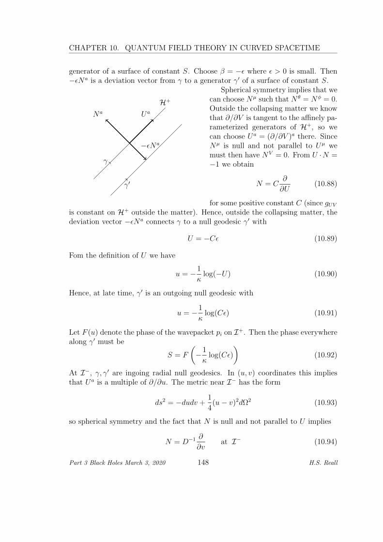
CHAPTER 10. QUANTUM FIELD THEORY IN CURVED SPACETIME
generator of a surface of constant S. Choose β = −ε where ε > 0 is small. Then−εNa is a deviation vector from γ to a generator γ′ of a surface of constant S.
H+
γ
γ′
Na Ua
−εNa
Spherical symmetry implies that wecan choose Nµ such that N θ = Nφ = 0.Outside the collapsing matter we knowthat ∂/∂V is tangent to the affinely pa-rameterized generators of H+, so wecan choose Ua = (∂/∂V )a there. SinceNµ is null and not parallel to Uµ wemust then have NV = 0. From U ·N =−1 we obtain
N = C∂
∂U(10.88)
for some positive constant C (since gUVis constant on H+ outside the matter). Hence, outside the collapsing matter, thedeviation vector −εNa connects γ to a null geodesic γ′ with
U = −Cε (10.89)
Fom the definition of U we have
u = −1
κlog(−U) (10.90)
Hence, at late time, γ′ is an outgoing null geodesic with
u = −1
κlog(Cε) (10.91)
Let F (u) denote the phase of the wavepacket pi on I+. Then the phase everywherealong γ′ must be
S = F
(−1
κlog(Cε)
)(10.92)
At I−, γ, γ′ are ingoing radial null geodesics. In (u, v) coordinates this impliesthat Ua is a multiple of ∂/∂u. The metric near I− has the form
ds2 = −dudv +1
4(u− v)2dΩ2 (10.93)
so spherical symmetry and the fact that N is null and not parallel to U implies
N = D−1 ∂
∂vat I− (10.94)
Part 3 Black Holes March 3, 2020 148 H.S. Reall

10.7. HAWKING RADIATION
for some positive constant D, which implies that γ′ intersects I− at
v = −D−1ε (10.95)
Combining with (10.92), we learn that the phase on I− is, for small v < 0,
S = F
(−1
κlog(−CDv)
)(10.96)
Hence on I− we have
p(2)i ≈
0 v > 0A(v) exp
[iF(− 1κ
log(−CDv))]
small v < 0(10.97)
where the amplitude A(v) is a smooth positive function. This shows that, on I−,most of our late time wavepacket is squeezed into a small region near v = 0 wherethe logarithm varies rapidly. To determine Bij we now have to decompose thisfunction into positive and negative frequency ”in” modes on I−.
So far we have been working with normalizable wavepackets built by superpos-ing modes of definite frequency. But now we will assume that pi contains only thesingle positive frequency ωi > 0 so F (u) = −ωiu. This means that pi is neithernormalizable nor localized at late time (as assumed above) but it makes the rest ofthe calculation easier. The result is the same as a more rigorous calculation usingwavepackets. We will also use ω to label the modes i.e. we will write pω insteadof pi (there will be additional labels (l,m) but we will suppress these). For thisfunction pω we have on I−:
p(2)ω ≈
0 v > 0Aω(v) exp
[iωκ
log(−CDv)]
small v < 0(10.98)
Similarly we will use a basis of ”in” modes fσ such that fσ has frequency σ > 0,i.e., fσ = (2πNσ)−1e−iσv on I− where Nσ is a normalization constant. Writing p
(2)ω
in terms of fσ, fσ is therefore just a Fourier transform w.r.t. v on I−. Since p(2)ω
is squeezed into a small range of v near v = 0 (or would be if it were a wavepacket),its Fourier transform will involve mainly high frequency modes, i.e. large σ. Forsuch modes, the Fourier transform is dominated by the region where p
(2)ω oscillates
most rapidly, i.e., near v = 0. So we can use the above expression and approximatethe amplitude Ai(v) as a constant. The Fourier transform is therefore
p(2)ω (σ) = Aω
∫ 0
−∞dv eiσv exp
[iω
κlog(−CDv)
](10.99)
with inverse
p(2)ω (v) =
∫ ∞−∞
dσ
2πe−iσvp(2)
ω (σ) (10.100)
=
∫ ∞0
dσNσp(2)ω (σ)fσ(v) +
∫ ∞0
dσNσp(2)ω (−σ)fσ(v)
Part 3 Black Holes March 3, 2020 149 H.S. Reall

CHAPTER 10. QUANTUM FIELD THEORY IN CURVED SPACETIME
R→∞
Figure 10.7: Choice of contour in complex v-plane.
the first term picks out the positive frequency components and second term thenegative frequency components. Hence in (10.80) we have
A(2)ωσ = Nσp
(2)ω (σ) Bωσ = Nσp
(2)ω (−σ) ω, σ > 0 (10.101)
The integral in (10.99) is not convergent but this is an artefact of working withnon-normalizable states. It would converge if we used wavepackets so we willmanipulate it as if it converged. We will want to extend the integrand into thecomplex v-plane so we define the logarithm with a branch cut in the lower halfplane:
log z = log |z|+ i arg z arg z ∈ (−π/2, 3π/2) (10.102)
which makes the integrand in (10.99) analytic in the lower half plane. If σ > 0 then
the integrand in p(2)ω (−σ) decays as v → ∞ in the lower half v-plane. Consider
the semi-circular contour shown in Fig. 10.7. The integral around this contourvanishes by Cauchy’s theorem. The integral around the curved part of the semi-circle vanishes as R→∞ (at least it would if we were working with wavepackets,by Jordan’s lemma). Hence we have, for σ > 0
p(2)ω (−σ) = −Aω
∫ ∞0
dv e−iσv exp[iω
κlog(−CDv)
]= −Aω
∫ ∞0
dv e−iσv exp[iω
κ(log(CDv) + iπ)
]= −Aωe−ωπ/κ
∫ 0
−∞dv eiσv exp
[iω
κlog(−CDv)
]= −e−ωπ/κp(2)
ω (σ) (10.103)
therefore|Bωσ| = e−ωπ/κ|A(2)
ωσ| (10.104)
Part 3 Black Holes March 3, 2020 150 H.S. Reall

10.7. HAWKING RADIATION
We now return to using wavepackets, for which the corresponding result is
|Bij| = e−ωiπ/κ|A(2)ij | (10.105)
Now the normalization of p(2) gives (upon substituting in the decomposition of p(2)
in terms of f, f)
T 2i = (p
(2)i , p
(2)i ) =
∑j
(|A(2)
ij |2 − |Bij|2)
=(e2ωiπ/κ − 1
)∑j
|Bij|2
=(e2ωiπ/κ − 1
)(BB†)ii (10.106)
hence the expected number of late time ”out” particles of type i is
〈0|b†ibi|0〉 =Γi
(e2ωiπ/κ − 1)(10.107)
where Γi ≡ T 2i . As explained above, Γi is the ”absorption cross-section” for the
mode fi (the ”in” mode with the same profile as the ”out mode” pi), i.e., thefraction of this mode that is absorbed by the black hole. This result is exactly thespectrum of a blackbody at the Hawking temperature
TH =κ
2π(10.108)
This result shows that particle production is not just a transient effect duringgravitational collapse: surprisingly, there is a steady flux of particles at late time.
The above argument can be generalized to other types of free field e.g. amassive scalar field, an electromagnetic field or a fermion field. In all cases, theresult is the same: a blackbody spectrum at the Hawking temperature. One canalso generalize to allow for non-spherically symmetric collapse, and collapse to arotating or charged black hole. In the latter cases, one finds that the temperatureis still given by (10.108) and the black hole preferentially emits particles with thesame sign angular momentum or charge as itself, just like a rotating or chargedblackbody.
For an astrophysical black hole, the Hawking temperature is tiny: for Schwarzschildwe have
TH = 6× 10⁻⁸MM
K (10.109)
this is well below the temperature of the cosmic microwave background radiation(2.7K) so astrophysical black holes absorb much more radiation from the CMBthan they emit in Hawking radiation, Tiny black holes, with M M, couldhave a non-negligible temperature. But there is no convincing evidence for theexistence of such small black holes.
Notice that TH decreases with M . So Schwarzschild black holes have negativeheat capacity.
Part 3 Black Holes March 3, 2020 151 H.S. Reall
CHAPTER 10. QUANTUM FIELD THEORY IN CURVED SPACETIME
10.8 Black hole thermodynamics
Hawking’s discovery implies that a stationary black hole is a thermodynamic ob-ject with temperature TH . Hence the zeroth law of black hole mechanics can beregarded as the zeroth law of thermodynamics applied to a black hole (the tem-perature is constant throughout a body in thermal equilibrium). ‘The first law ofblack hole mechanics can now be written
dE = THdSBH + ΩHdJ (10.110)
where
SBH =A
4(10.111)
This is identical in form to the first law of thermodynamics provided we interpretSBH as the entropy of the black hole: this is referred to as the Bekenstein-Hawkingentropy. Reinstating units we have
SBH =c3A
4G~(10.112)
The second law of black hole mechanics now states that SBH is non-decreasingclassically. But SBH does decrease quantum mechanically by Hawking radiation:the black hole loses energy by emitting radiation and therefore gets smaller. How-ever, this radiation itself has entropy and the total entropy Sradiation +SBH does notdecrease. This is a special case of the generalized second law (due to Bekenstein)which states that the total entropy
S = Smatter + SBH (10.113)
is non-decreasing in any physical process. Evidence in favour of this law comesfrom the failure of various thought experiments aimed at violating it.
The result that black holes have entropy has several consequences. First,plugging in numbers reveals that the entropy of a Schwarzschild black hole withM = M is SBH ∼ 1077. This is many orders of magnitude greater than theentropy of the matter in the Sun: S ∼ 1058. Hence the entropy of the Universewould be much greater if all of the mass were in the form of black holes. So ourUniverse is in a very special (i.e. low entropy) state. This observation is due toPenrose.
Second, Hawking’s result treats the gravitational field classically. But sta-tistical physics tells us that entropy measures how many quantum microstatescorrespond to the same macroscopic configuration. So a black hole must haveN ∼ exp(A/4) quantum microstates. What are these? To answer this requiresa quantum theory of gravity. A statistical physics derivation of SBH = A/4 is a
Part 3 Black Holes March 3, 2020 152 H.S. Reall

10.9. BLACK HOLE EVAPORATION
major goal of quantum gravity research. String theory has been successful in do-ing this for certain ”supersymmetric” black holes. Such black holes are necessarilyextreme (κ = 0) and include the extreme Reissner-Nordstrom solution.
10.9 Black hole evaporation
The energy of the Hawking radiation must come from the black hole itself. Hawk-ing’s calculation neglects the effect of the radiation on the spacetime geometry. Anaccurate calculation of this backreaction would involve quantum gravity. However,one can estimate the rate of mass loss by using Stefan’s law for the rate of energyloss by a blackbody:
dE
dt≈ −αAT 4 (10.114)
where α is a dimensionless constant and we approximate Γi by treating the blackhole as a perfectly absorbing sphere of area A (roughly the black hole horizon area)in Minkowski spacetime. Plugging in E = M with A ∝ M2 and T ∝ 1/M givesdM/dt ∝ −1/M2. Hence the black hole evaporates away completely in a time
τ ∼M3 ∼ 1071
(M
M
)3
sec (10.115)
This is a very crude calculation but it is expected to be a reasonable approximationat least until the size of the black hole becomes comparable to the Planck mass (1in our units) when quantum gravity effects are expected to become important.
This process of black hole evaporation leads to the information paradox. Con-sider gravitational collapse of matter to form a black hole which then evaporatesaway completely, leaving thermal radiation. It should be possible to arrange thatthe collapsing matter is in a definite quantum state, i.e., a pure state rather thana density matrix. However, the final state is a mixed state, i.e., only describablein terms of a density matrix. Evolution from a pure state to a mixed state isimpossible according to the usual unitary time evolution in quantum mechanics.
Another way of saying this is: information about the initial state appears to bepermanently lost in black hole formation and evaporation. This is in contrast with,say, burning an encyclopaedia. In that case one could reproduce (in principle) theinformation in the encyclopaedia if one collected all of the radiation and ashes andstudied them very carefully. Not so with Hawking radiation, which appears to beexactly thermal and hence contains no information about the initial state apartfrom its mass, angular momentum and charge.
Hawking interpreted this apparent paradox as indicating that quantum me-chanics would need modifying in a full quantum theory of gravity. Most otherphysicists take a more conservative view that information is not really lost and
Part 3 Black Holes March 3, 2020 153 H.S. Reall

CHAPTER 10. QUANTUM FIELD THEORY IN CURVED SPACETIME
that there are subtle correlations in the Hawking radiation which take a long timeto appear but could, in principle, be used to reconstruct information about theinitial state. However, this idea has run into trouble recently: if one assumes this,as well as several other cherished beliefs about black hole physics (e.g. nothingspecial happens at the event horizon, QFT in curved spacetime is a good descrip-tion of the physics until the black hole reaches the Planck scale) then one runsinto a contradiction (Almheiri, Marolf, Polchinski & Sully 2012).
Part 3 Black Holes March 3, 2020 154 H.S. Reall
Related Documents