Part 21: Generalized Method of Moments 1-1/67 Econometrics I Professor William Greene Stern School of Business Department of Economics

Part 21: Generalized Method of Moments 21-1/67 Econometrics I Professor William Greene Stern School of Business Department of Economics.
Dec 22, 2015
Welcome message from author
This document is posted to help you gain knowledge. Please leave a comment to let me know what you think about it! Share it to your friends and learn new things together.
Transcript

Part 21: Generalized Method of Moments21-1/67
Econometrics IProfessor William Greene
Stern School of Business
Department of Economics

Part 21: Generalized Method of Moments21-2/67
Econometrics I
Part 21 – GeneralizedMethod of Moments
Part 21: Generalized Method of Moments21-3/67
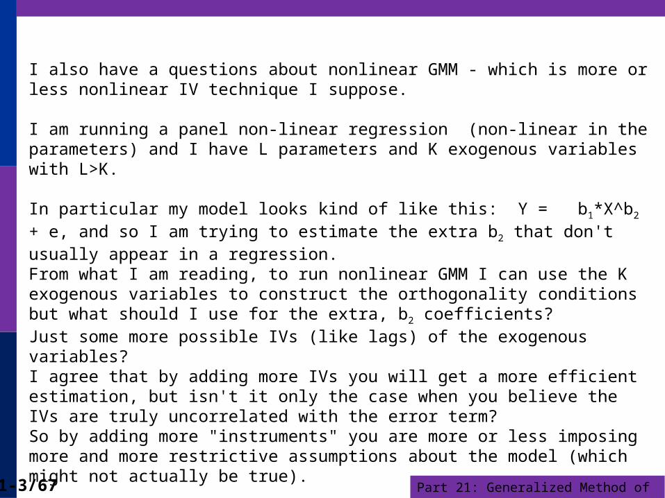
I also have a questions about nonlinear GMM - which is more or less nonlinear IV technique I suppose.
I am running a panel non-linear regression (non-linear in the parameters) and I have L parameters and K exogenous variables with L>K.
In particular my model looks kind of like this: Y = b1*X^b2 + e, and so I am trying to estimate the extra b2 that don't usually appear in a regression.From what I am reading, to run nonlinear GMM I can use the K exogenous variables to construct the orthogonality conditions but what should I use for the extra, b2 coefficients?Just some more possible IVs (like lags) of the exogenous variables?I agree that by adding more IVs you will get a more efficient estimation, but isn't it only the case when you believe the IVs are truly uncorrelated with the error term?So by adding more "instruments" you are more or less imposing more and more restrictive assumptions about the model (which might not actually be true).
I am asking because I have not found sources comparing nonlinear GMM/IV to nonlinear least squares. If there is no homoscadesticity/serial correlation what is more efficient/give tighter estimates?
Part 21: Generalized Method of Moments21-4/67
I’m trying to minimize a nonlinear program with the least square under nonlinear constraints. It’s first introduced by Ané & Geman (2000). It consisted on the minimization of the sum of squared difference between the moment generating function and the theoretical moment generating function
Part 21: Generalized Method of Moments21-5/67
2 212
2 2121
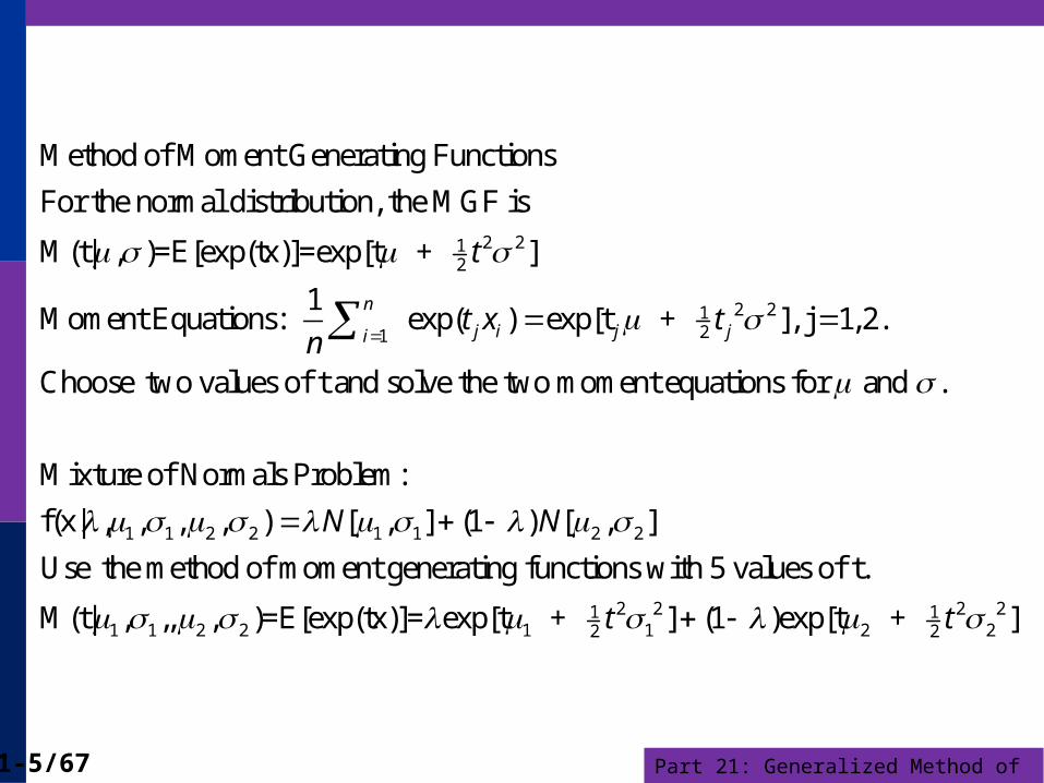
Method of Moment Generating Functions
For the normal distribution, the MGF is
M(t| , )=E[exp(tx)]=exp[t + ]
1Moment Equations: exp( ) exp[t + ], j 1, 2.
Choose two values of t
n
j i j ji
t
t x tn
1 1 2 2 1 1 2 2
1 1 2 2
and solve the two moment equations for and .
Mixture of Normals Problem:
f(x| , , , , ) [ , ] (1 ) [ , ]
Use the method of moment generating functions with 5 values of t.
M(t| , ,, , )=E
N N
2 2 2 21 11 1 2 22 2[exp(tx)]= exp[t + ] (1 )exp[t + ]t t

Part 21: Generalized Method of Moments21-6/67
1 1 21
1 1 2 2
5 2 2 2 21 11 1 2 22 21
Finding the solutions to the moment equations: Least squares
1M̂(t ) exp( ), and likewise for t ,...
Minimize( , , , , )
M̂(t ) exp[t + ] (1 )exp[t + ]
Altern
n
ii
jj
t xn
t t
1 1 2 2 1 1 2 21
ative estimator: Maximum Likelihood
L( , , , , ) log [x | , ] (1 ) [x | , ]N
i iiN N
Part 21: Generalized Method of Moments21-7/67
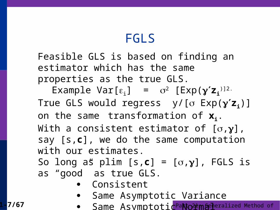
FGLSFeasible GLS is based on finding an estimator which has the same properties as the true GLS.
Example Var[i] = 2 [Exp(zi)]2.
True GLS would regress y/[ Exp(zi)] on the same transformation of xi.With a consistent estimator of [,], say [s,c], we do the same computation with our estimates.So long as plim [s,c] = [,], FGLS is as “good” as true GLS. Consistent Same Asymptotic Variance Same Asymptotic Normal Distribution
Part 21: Generalized Method of Moments21-8/67
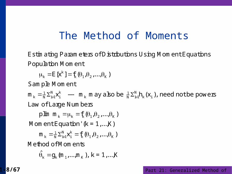
The Method of Moments
kk k 1 2 K
N k N1 1k i 1 i k i 1 k iN N
Estimating Parameters of Distributions Using Moment Equations
Population Moment
E[x ] f ( , ,..., )
Sample Moment
m x --- m may also be h (x ), need not be powers
Law of L
k k k 1 2 K
N k1k i 1 i k 1 2 KN
k k 1 K
arge Numbers
plim m f ( , ,..., )
'Moment Equation' (k = 1,...,K)
m x f ( , ,..., )
Method of Moments
ˆ g (m ,...,m ), k = 1,...,K

Part 21: Generalized Method of Moments21-9/67
Estimating a Parameter
Mean of Poisson p(y)=exp(-λ) λy / y! E[y]= λ.
plim (1/N)Σiyi = λ. This is the estimator
Mean of Exponential p(y) = λ exp(- λy) E[y] = 1/ λ.
plim (1/N)Σiyi = 1/λ

Part 21: Generalized Method of Moments21-10/67
Mean and Variance of a Normal Distribution
2
2
2 2 2
N N 2 2 21 1i 1 i i 1 iN N
2 N 2 2 N 21 1i 1 i i 1 iN n
1 (y )p(y) exp
22
Population Moments
E[y] , E[y ]
Moment Equations
y , y
Method of Moments Estimators
ˆ=y, ˆ y (y ) (y y)

Part 21: Generalized Method of Moments21-11/67
Gamma DistributionP P 1
22
exp( y)yp(y)
(P)
PE[y]
P(P 1)E[y ]
E[1/ y]P 1
E[logy] (P) log , (P)=dln (P)/dP
(Each pair gives a different answer. Is there a 'best' pair? Yes,
the ones that are 'sufficient' statistics.
E[y] and E[logy]. For a
different course....)
Part 21: Generalized Method of Moments21-12/67
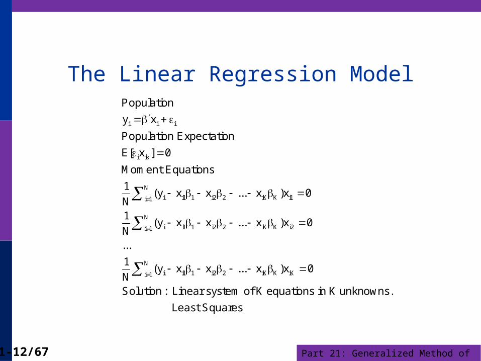
The Linear Regression Model
i i i
i ik
N
i i1 1 i2 2 iK K i1i 1
N
i i1 1 i2 2 iK K i2i 1
N
i i1 1 i2 2 iK K iKi 1
Population
y x
Population Expectation
E[ x ] 0
Moment Equations
1(y x x ... x )x 0
N1
(y x x ... x )x 0N...
1(y x x ... x )x 0
NSolution : Linea
r system of K equations in K unknowns.
Least Squares

Part 21: Generalized Method of Moments21-13/67
Instrumental Variables
i i i
i ik 1 K
N
i i1 1 i2 2 iK K i1i 1
N
i i1 1 i2 2 iK K i2i 1
i i1 1i 1
Population
y x
Population Expectation
E[ z ] 0 for instrumental variables z ... z .
Moment Equations
1(y x x ... x )z 0
N1
(y x x ... x )z 0N...
1(y x
N
N
i2 2 iK K iK
-1IV
x ... x )z 0
Solution : Also a linear system of K equations in K unknowns.
b = ( )
Z'X Z'y/n ( /n)
Part 21: Generalized Method of Moments21-14/67
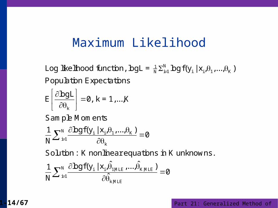
Maximum Likelihood
N1i 1 i i 1 KN
k
N i i 1 Ki 1
k
Log likelihood function, logL = logf(y | x , ,..., )
Population Expectations
logLE 0, k = 1,...,K
Sample Moments
logf(y | x , ,..., )10
N
Solution : K nonlinear equations in K un
N i i 1,MLE K,MLE
i 1k,MLE
knowns.
ˆ ˆlogf(y | x , ,..., )10
ˆN

Part 21: Generalized Method of Moments21-15/67
Behavioral Application
t 1t t
t
t
t
t+1 t 1 t
t t 1 t
Life Cycle Consumption (text, page 455)
c1E (1 r) 1 0
1 c
discount rate
c consumption
information at time t
Let =1/(1+ ), R c / c , =-
E [ (1 r)R 1| ] 0
What is in the information set? Each piece of 'information'
provides a moment equation for estimation of the two parameters.
Part 21: Generalized Method of Moments21-16/67
Identification Can the parameters be estimated? Not a sample ‘property’ Assume an infinite sample
Is there sufficient information in a sample to reveal consistent estimators of the parameters
Can the ‘moment equations’ be solved for the population parameters?
Part 21: Generalized Method of Moments21-17/67
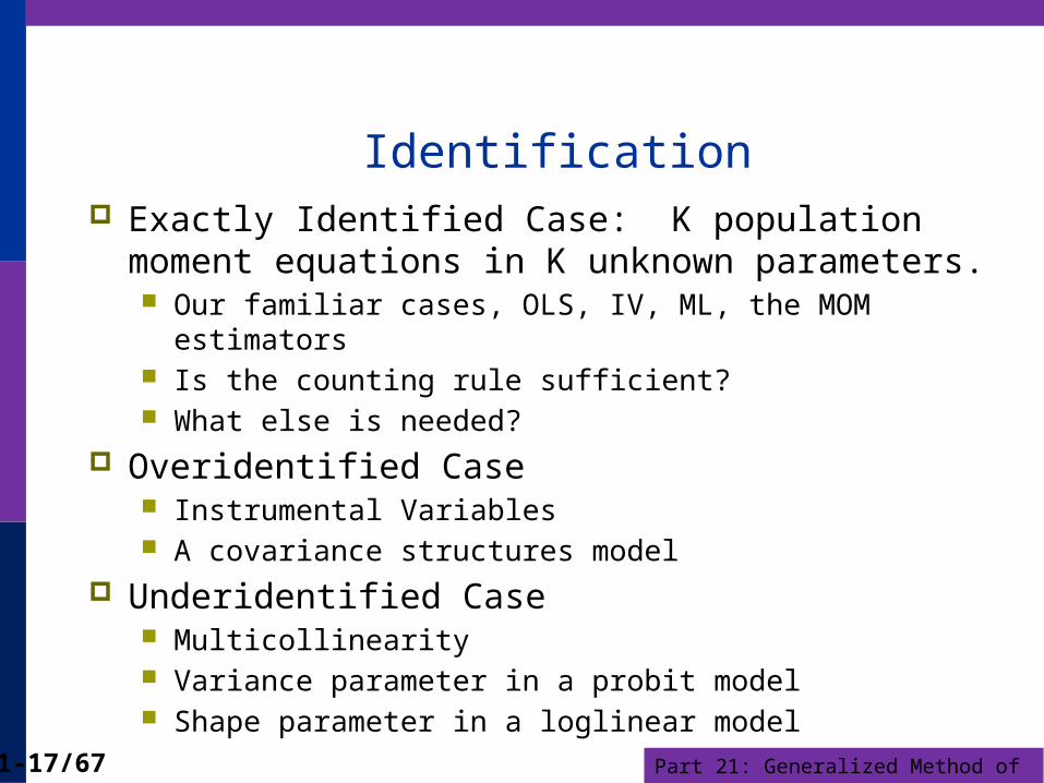
Identification Exactly Identified Case: K population moment equations
in K unknown parameters. Our familiar cases, OLS, IV, ML, the MOM estimators Is the counting rule sufficient? What else is needed?
Overidentified Case Instrumental Variables A covariance structures model
Underidentified Case Multicollinearity Variance parameter in a probit model Shape parameter in a loglinear model
Part 21: Generalized Method of Moments21-18/67
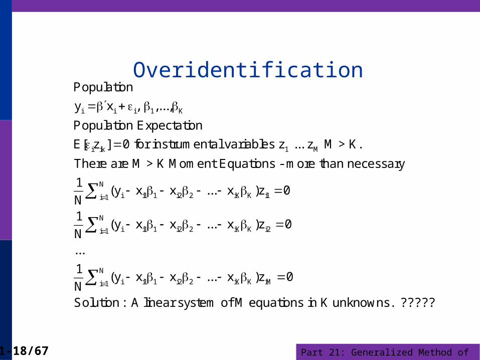
Overidentification
i i i 1 K
i ik 1 M
N
i i1 1 i2 2 iK K i1i 1
Population
y x , ,...,
Population Expectation
E[ z ] 0 for instrumental variables z ... z M > K.
There are M > K Moment Equations - more than necessary
1(y x x ... x )z 0
N1
N
i i1 1 i2 2 iK K i2i 1
N
i i1 1 i2 2 iK K iMi 1
(y x x ... x )z 0N...
1(y x x ... x )z 0
NSolution : A linear system of M equations in K unknowns. ?????
Part 21: Generalized Method of Moments21-19/67
Overidentification
1 1 1
2 2 2
1 1 1
2 2 2
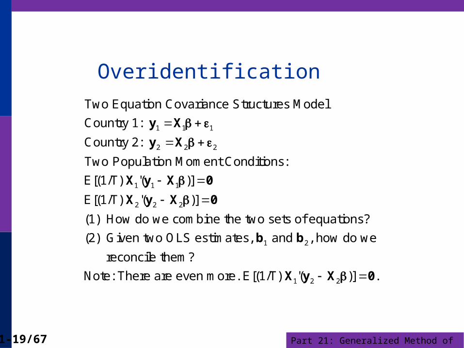
Two Equation Covariance Structures Model
Country 1:
Country 2:
Two Population Moment Conditions:
E[(1/T) '( )]
E[(1/T) '( )]
(1) How do we combine the two sets of eq
y X
y X
X y X 0
X y X 0
1 2
1 2 2
uations?
(2) Given two OLS estimates, and , how do we
reconcile them?
Note: There are even more. E[(1/T) '( )] .
b b
X y X 0
Part 21: Generalized Method of Moments21-20/67
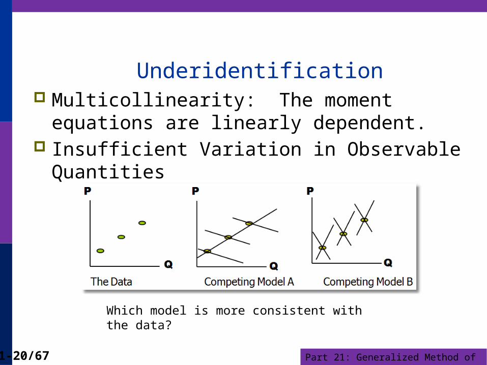
Underidentification Multicollinearity: The moment equations are
linearly dependent. Insufficient Variation in Observable Quantities
Which model is more consistent with the data?

Part 21: Generalized Method of Moments21-21/67
Underidentification – Model/Data
z
x
i i i
i i 0 i0
i
Consider the Mover - Stayer Model
Binary choice for whether an individual 'moves' or 'stays'
d 1( u 0)
Outcome equation for the individual, conditional on the state:
y | (d 0) =
y | (d 1)
xi 1 i1
2 2i0 i1 0 1 0 1
=
( , ) ~N[(0,0),( , , )]
An individual either moves or stays, but not both (or neither).
The parameter cannot be estimated with the observed data
regardless of the sample size.
It is unidentified.

Part 21: Generalized Method of Moments21-22/67
Underidentification - Math
0
0 1
1
0 1
When a parameter is unidentified, the log likelihood is invariant
to changes in it. Consider the logit binary choice model
exp( x)Prob[y=0]=
exp( x) exp( x)
exp( x)Prob[y=1]=
exp( x) exp( x)
Probabil
0 0
0 1 0 1
1 1
0 1 0
ities sum to 1, are monotonic, etc. But, consider, for any 0,
exp[( )x] exp( x)Prob[y=0]=
exp[( )x] exp[( )x] exp( x) exp( x)
exp[( )x] exp( x)Prob[y=1]=
exp[( )x] exp[( )x] exp( x
1
0
) exp( x)
The parameters are unidentified. A normalization such as 0 is needed.
Part 21: Generalized Method of Moments21-23/67
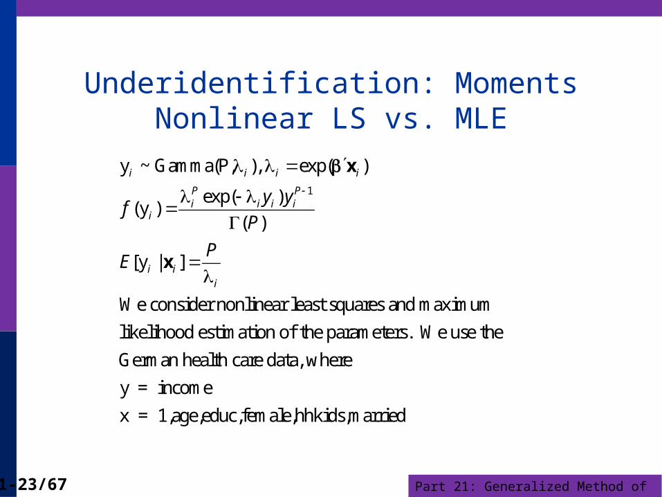
Underidentification: MomentsNonlinear LS vs. MLE
1
y ~ Gamma(P, ), exp( )
exp( )(y )
( )
[y | ]
We consider nonlinear least squares and maximum
likelihood estimation of the parameters. We use the
German health care data, where
y
i i i i
P Pi i i i
i
i ii
y yf
P
PE
x
x
= income
x = 1,age,educ,female,hhkids,married
Part 21: Generalized Method of Moments21-24/67
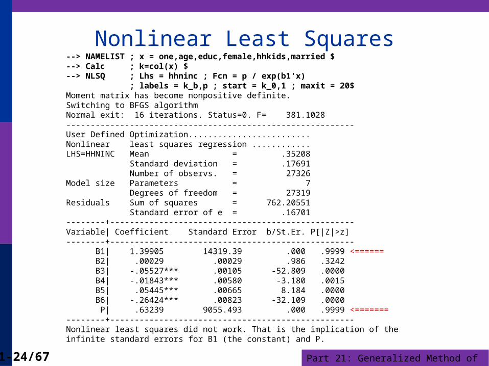
Nonlinear Least Squares--> NAMELIST ; x = one,age,educ,female,hhkids,married $--> Calc ; k=col(x) $--> NLSQ ; Lhs = hhninc ; Fcn = p / exp(b1'x) ; labels = k_b,p ; start = k_0,1 ; maxit = 20$Moment matrix has become nonpositive definite.Switching to BFGS algorithmNormal exit: 16 iterations. Status=0. F= 381.1028-----------------------------------------------------------User Defined Optimization.........................Nonlinear least squares regression ............LHS=HHNINC Mean = .35208 Standard deviation = .17691 Number of observs. = 27326Model size Parameters = 7 Degrees of freedom = 27319Residuals Sum of squares = 762.20551 Standard error of e = .16701--------+--------------------------------------------------Variable| Coefficient Standard Error b/St.Er. P[|Z|>z]--------+-------------------------------------------------- B1| 1.39905 14319.39 .000 .9999 <====== B2| .00029 .00029 .986 .3242 B3| -.05527*** .00105 -52.809 .0000 B4| -.01843*** .00580 -3.180 .0015 B5| .05445*** .00665 8.184 .0000 B6| -.26424*** .00823 -32.109 .0000 P| .63239 9055.493 .000 .9999 <=======--------+--------------------------------------------------Nonlinear least squares did not work. That is the implication of theinfinite standard errors for B1 (the constant) and P.
Part 21: Generalized Method of Moments21-25/67
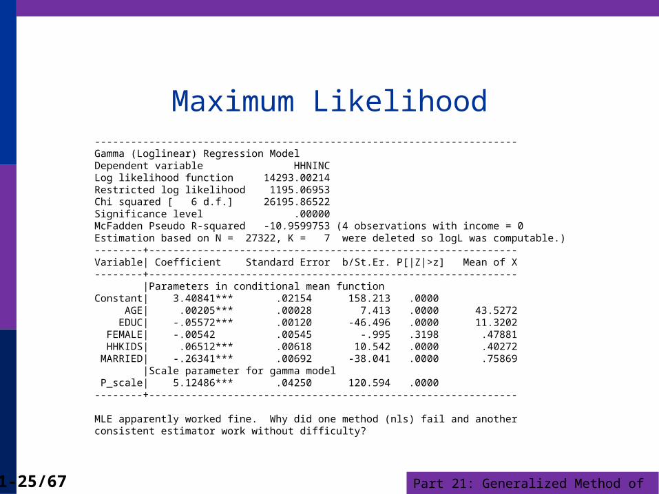
Maximum Likelihood----------------------------------------------------------------------Gamma (Loglinear) Regression ModelDependent variable HHNINCLog likelihood function 14293.00214Restricted log likelihood 1195.06953Chi squared [ 6 d.f.] 26195.86522Significance level .00000McFadden Pseudo R-squared -10.9599753 (4 observations with income = 0Estimation based on N = 27322, K = 7 were deleted so logL was computable.)--------+-------------------------------------------------------------Variable| Coefficient Standard Error b/St.Er. P[|Z|>z] Mean of X--------+------------------------------------------------------------- |Parameters in conditional mean functionConstant| 3.40841*** .02154 158.213 .0000 AGE| .00205*** .00028 7.413 .0000 43.5272 EDUC| -.05572*** .00120 -46.496 .0000 11.3202 FEMALE| -.00542 .00545 -.995 .3198 .47881 HHKIDS| .06512*** .00618 10.542 .0000 .40272 MARRIED| -.26341*** .00692 -38.041 .0000 .75869 |Scale parameter for gamma model P_scale| 5.12486*** .04250 120.594 .0000--------+-------------------------------------------------------------
MLE apparently worked fine. Why did one method (nls) fail and another consistent estimator work without difficulty?

Part 21: Generalized Method of Moments21-26/67
Moment Equations: NLS
2
1 1
1
1
1
[ | ] / exp( )
' / exp( )
2'0
exp( )
2'
exp( )
Consider the term for the constant in the model, . Notice that
the first order condition for
i
N N
i i ii i
N ii
i
N iii
i
E y P
y P e
e
P
e P
x x
e e x
e e
x
e ex 0
x
1
1
the constant term is
20. This doesn't depend on P, since we can divide
exp( )
both sides of the equation by P. This means that we cannot find
solutions for both and P. It is easy to see
N ii
i
e P
x
1 1
1
why NLS cannot distinguish
P from . E[y|x] = exp((logP- ) ...). There are an infinite number
of pairs of (P, ) that produce the same constant term in the model.
Part 21: Generalized Method of Moments21-27/67
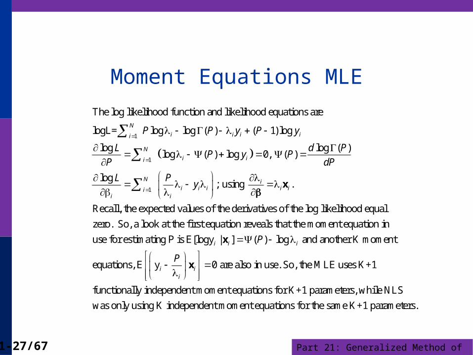
Moment Equations MLE
1
1
1
The log likelihood function and likelihood equations are
logL= log log ( ) ( 1) log
log log ( )log ( ) log 0, ( )
log; using .
Recall
N
i i i ii
N
i ii
N ii i i i ii
i i
P P y P y
L d PP y P
P dP
L Py
x
, the expected values of the derivatives of the log likelihood equal
zero. So, a look at the first equation reveals that the moment equation in
use for estimating P is E[logy | ] ( ) log and anothei i iP x r K moment
equations, E y 0 are also in use. So, the MLE uses K+1
functionally independent moment equations for K+1 parameters, while NLS
was only using K independent moment equation
i ii
P
x
s for the same K+1 parameters.
Part 21: Generalized Method of Moments21-28/67
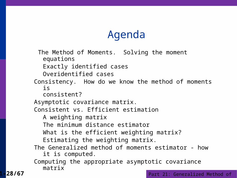
Agenda
The Method of Moments. Solving the moment equationsExactly identified casesOveridentified cases
Consistency. How do we know the method of moments is consistent?
Asymptotic covariance matrix.Consistent vs. Efficient estimation
A weighting matrixThe minimum distance estimatorWhat is the efficient weighting matrix?Estimating the weighting matrix.
The Generalized method of moments estimator - how it is computed.Computing the appropriate asymptotic covariance matrix

Part 21: Generalized Method of Moments21-29/67
The Method of MomentsMoment Equation: Defines a sample statistic that
mimics a population expectation:
The population expectation – orthogonality condition:
E[ mi () ] = 0. Subscript i indicates it depends on data vector indexed by 'i' (or 't' for a time series setting)

Part 21: Generalized Method of Moments21-30/67
The Method of Moments - Example
P P 1i i
i
i i
N1 i=1 i
N2 i=1 i
Gamma Distribution Parameters
exp( y )yp(y )
(P)
Population Moment Conditions
PE[y ] , E[logy ] (P) log
Moment Equations:
E[m ( ,P)] = E[{(1/n) y } P / ] 0
E[m ( ,P)] = E[{(1/n) logy } (
(P) log )] 0

Part 21: Generalized Method of Moments21-31/67
Application
2 21 1 2 2
2 21 2
1
2
Solving the moment equations
Use least squares:
Minimize {m E[m ]} {m E[m ]}
(m (P / )) (m ( (P) log ))
m 31.278
m 3.221387
Plot of Psi(P) Function
P
-10
-8
-6
-4
-2
0
2
-12
1 2 3 4 5 60
PSI
Part 21: Generalized Method of Moments21-32/67
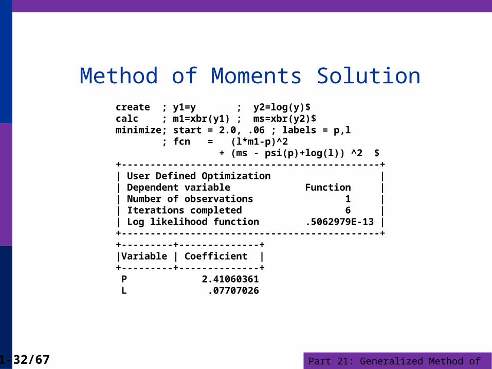
Method of Moments Solutioncreate ; y1=y ; y2=log(y)$calc ; m1=xbr(y1) ; ms=xbr(y2)$minimize; start = 2.0, .06 ; labels = p,l ; fcn = (l*m1-p)^2 + (ms - psi(p)+log(l)) ^2 $+---------------------------------------------+| User Defined Optimization || Dependent variable Function || Number of observations 1 || Iterations completed 6 || Log likelihood function .5062979E-13 |+---------------------------------------------++---------+--------------+ |Variable | Coefficient | +---------+--------------+ P 2.41060361 L .07707026
Part 21: Generalized Method of Moments21-33/67
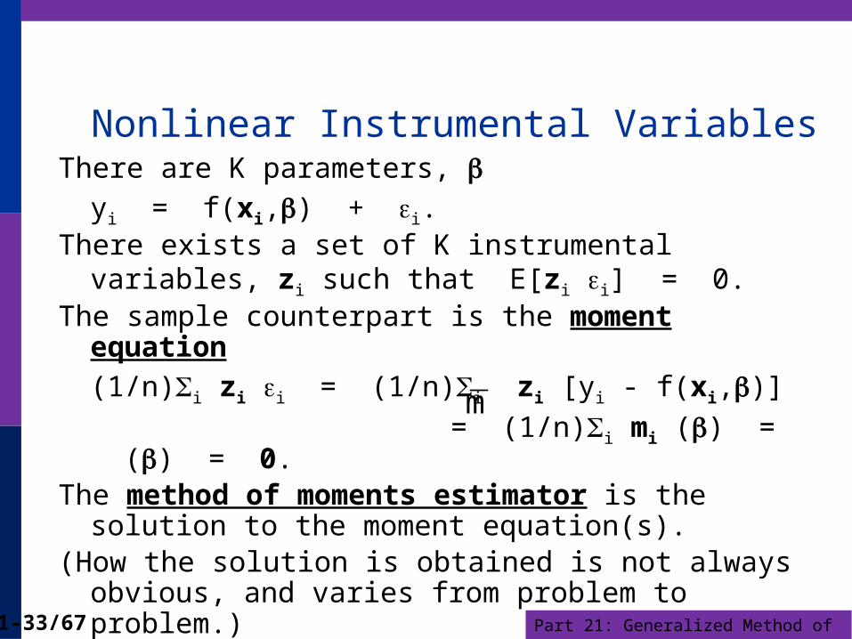
Nonlinear Instrumental VariablesThere are K parameters,
yi = f(xi,) + i.
There exists a set of K instrumental variables, zi such that E[zi i] = 0.
The sample counterpart is the moment equation
(1/n)i zi i = (1/n)i zi [yi - f(xi,)] = (1/n)i mi () = () = 0.The method of moments estimator is the solution to the
moment equation(s). (How the solution is obtained is not always obvious, and
varies from problem to problem.)
m
Part 21: Generalized Method of Moments21-34/67
The MOM Solution
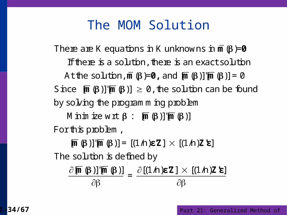
There are K equations in K unknowns in ( )=
If there is a solution, there is an exact solution
At the solution, ( )= and [ ( )]'[ ( )] = 0
Since [ ( )]'[ ( )] 0, the solution can be fou
m 0
m 0, m m
m m
nd
by solving the programming problem
Minimize wrt : [ ( )]'[ ( )]
For this problem,
[ ( )]'[ ( )] = [(1/n) ] [(1/n) ]
The solution is defined by
[ ( )]'[ ( )] [(1/n) ] =
m m
m m
m m
ε'Z Z'ε
ε'Z [(1/n) ]
Z'ε
Part 21: Generalized Method of Moments21-35/67
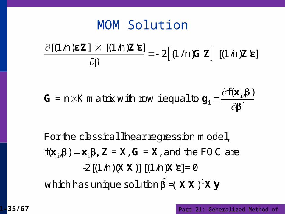
MOM Solution
ii
i i
[(1/n) ] [(1/n) ]2 (1/ n) [(1/n) ]
f( , ) = n K matrix with row i equal to
For the classical linear regression model,
f( , ) ' = , = , and the FOC are
-2[(1
xG g
x x Z X G X
ε'Z Z'εG'Z Z'ε
/n)( )] [(1/n) '
ˆ
X'X X
X'X X'y
ε-1
] = 0
which has unique solution =( )

Part 21: Generalized Method of Moments21-36/67
Variance of the Method of Moments Estimator
n
ii 1
i i
-1 -1
The MOM estimator solves m( )=
1 1( )= ( ) so the variance is for some
n NGenerally, = E[ ( ) ( ) ]
The asymptotic covariance matrix of the estimator is
1Asy.Var[ ]=( ) ( ) w
N
0
MOM
β
m β m β Ω Ω
Ω m β m β '
β G Ω G'( )
here m β
G=β'

Part 21: Generalized Method of Moments21-37/67
Example 1: Gamma Distribution
2
n1 P1 i 1 in
n12 i 1 in
i i i
i i i
1 PN
i 1 1
m (y )
m (logy (P) log )
Var(y ) Cov(y ,logy )1 1Cov(y ,logy ) Var(logy )n n
1
n '(P)G
Part 21: Generalized Method of Moments21-38/67
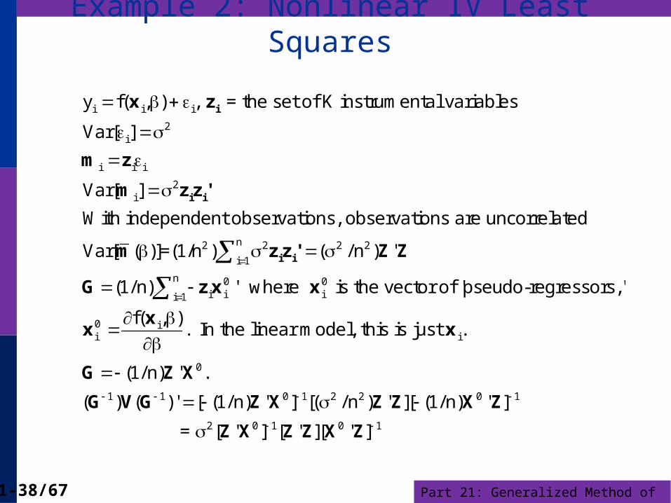
Example 2: Nonlinear IV Least Squares
i i i
2i
i i i
2i
n2 2 2 2
i 1
0i i
y f( , ) , = the set of K instrumental variables
Var[ ]
Var[ ]
With independent observations, observations are uncorrelated
Var[ ( )]=(1/n ) ( /n ) '
(1/n) '
i
i i
i i
x z
m z
m zz'
m zz' Z Z
G zx
n 0ii 1
0 ii i
0
1 1 0 1 2 2 0 1
2
where is the vector of 'pseudo-regressors,'
f( , ). In the linear model, this is just .
(1/n) ' .
( ) ( )' [ (1/n) ' ] [( / n ) ' ][ (1/n) ' ]
= [
x
xx x
G Z X
G V G Z X Z Z X Z
Z 0 1 0 1' ] [ ' ][ ' ]X Z Z X Z

Part 21: Generalized Method of Moments21-39/67
Variance of the Moments
i
n
i i i ii=1
n
i ii=1
How to estimate = (1/n) = Var[ ( )]
Var[ ( )]=(1/n)Var[ ( )] = (1/n)
Estimate Var[ ( )] with Est.Var[ ( )] = (1/n) ( ) ( )'
Then,
ˆ ˆ ˆ(1/ n) (1/ n) ( ) ( )'
For the linear regression
V m
m m
m m m m
V m m
i i i
n n 2i i i i i i ii=1 i=1
n-1 2 -1MOM i i ii=1
n-1 2 -1i i ii=1
model,
,
ˆ (1/ n) (1/ n) e e (1/ n) (1/ n) e
(1/ n)
Est.Var[b ] [(1/ n) ] [(1/ n) (1/ n) e ][(1/ n) ]
= [ ] [ e ][ ]
m x
V x x' x x'
G X'X
X'X x x' X'X
X'X x x' X'X (familiar?)

Part 21: Generalized Method of Moments21-40/67
Properties of the MOM Estimator Consistent?
The LLN implies that the moments are consistent estimators of their population counterparts (zero)
Use the Slutsky theorem to assert consistency of the functions of the moments
Asymptotically normal? The moments are sample means. Invoke a central limit theorem.
Efficient? Not necessarily Sometimes yes. (Gamma example) Perhaps not. Depends on the model and the available
information (and how much of it is used).
Part 21: Generalized Method of Moments21-41/67
Generalizing the Method of Moments Estimator
More moments than parameters – the overidentified case
Example: Instrumental variable case, M > K instruments

Part 21: Generalized Method of Moments21-42/67
Two Stage Least SquaresHow to use an “excess” of instrumental variables
(1) X is K variables. Some (at least one) of the K
variables in X are correlated with ε.
(2) Z is M > K variables. Some of the variables in
Z are also in X, some are not. None of the
variables in Z are correlated with ε.
(3) Which K variables to use to compute Z’X and
Z’y?

Part 21: Generalized Method of Moments21-43/67
Choosing the Instruments Choose K randomly? Choose the included Xs and the remainder randomly? Use all of them? How? A theorem: (Brundy and Jorgenson, ca. 1972) There is a
most efficient way to construct the IV estimator from this subset: (1) For each column (variable) in X, compute the predictions of
that variable using all the columns of Z. (2) Linearly regress y on these K predictions.
This is two stage least squares
Part 21: Generalized Method of Moments21-44/67
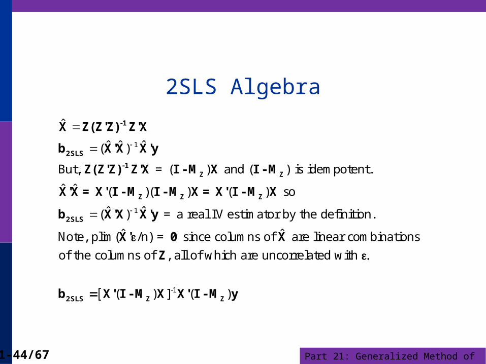
2SLS Algebra
1
1
ˆ
ˆ ˆ ˆ( )
But, = ( ) and ( ) is idempotent.
ˆ ˆ ( )( ) ( ) so
ˆ ˆ( ) = a real IV estimator by the definition.
ˆNote, plim( /n) =
-1
2SLS
-1Z Z
Z Z Z
2SLS
X Z(Z'Z) Z'X
b X'X X'y
Z(Z'Z) Z'X I -M X I -M
X'X= X' I -M I -M X= X' I -M X
b X'X X'y
X' 0
-1
ˆ since columns of are linear combinations
of the columns of , all of which are uncorrelated with
( ) ] ( )
2SLS Z Z
X
Z
b X' I -M X X' I -M y
Part 21: Generalized Method of Moments21-45/67
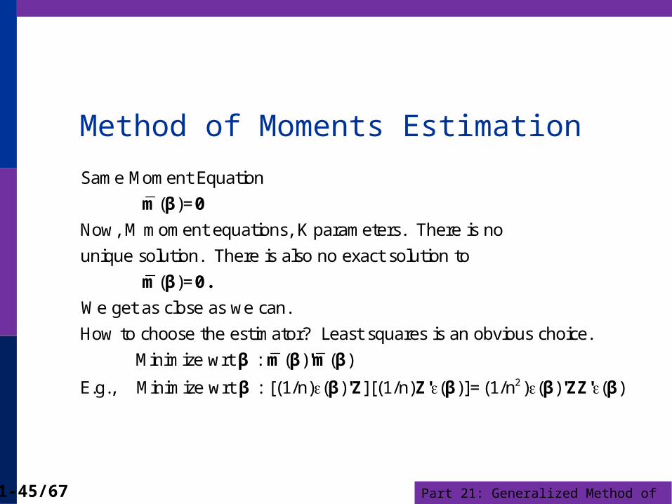
Method of Moments Estimation
m β 0
m β 0.
Same Moment Equation
( )=
Now, M moment equations, K parameters. There is no
unique solution. There is also no exact solution to
( )=
We get as close as we can.
How to cho
β m β 'm β
β β 'Z Z' β β 'ZZ' β2
ose the estimator? Least squares is an obvious choice.
Minimize wrt : ( ) ( )
E.g., Minimize wrt : [(1/n) ( ) ][(1/n) ( )]=(1/n ) ( ) ( )

Part 21: Generalized Method of Moments21-46/67
FOC for MOM
m β 'm β β= G β 'm β
β 'ZZ' β β = - X Z Z' y - Xβ
0
2 2
First order conditions
(1) General
( ) ( )/ 2 ( ) ( ) = 0
(2) The Instrumental Variables Problem
(1/n ) ( ) ( )/ (2/n )( ' )[ ( )]
=
Or,
X Z Z' y - Xβ 0
0
X Z Z' y - Xβ 0
Z' y - Xβ 0
( ' )[ ( )] =
(K M) (M N)(N 1) =
At the solution, ( ' )[ ( )] =
But, [ ( )] as it was before.

Part 21: Generalized Method of Moments21-47/67
Computing the Estimator
Programming Program No all purpose solution Nonlinear optimization problem –
solution varies from setting to setting.
Part 21: Generalized Method of Moments21-48/67
Asymptotic Covariance Matrix
-1
m β 0
G β 'm β 0 G β '
β G β ' V G β V= m-1
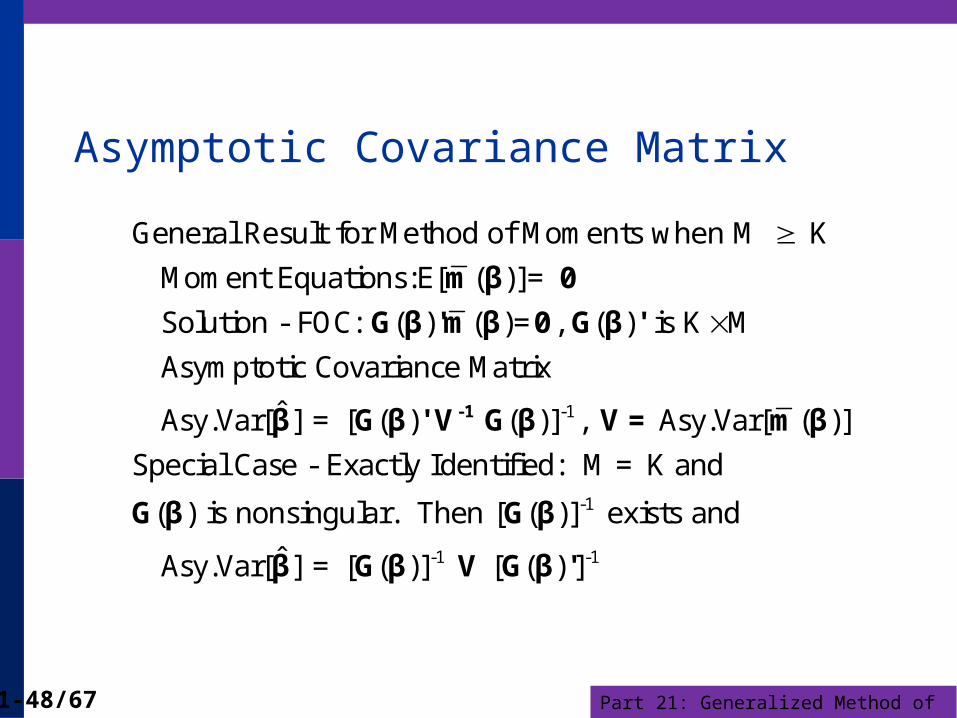
General Result for Method of Moments when M K
Moment Equations:E[ ( )]=
Solution - FOC: ( ) ( )= , ( ) is K M
Asymptotic Covariance Matrix
ˆ Asy.Var[ ] = [ ( ) ( )] , Asy.Var[ β
G β G β
β G β V G β '
-1
-1 -1
( )]
Special Case - Exactly Identified: M = K and
( ) is nonsingular. Then [ ( )] exists and
ˆ Asy.Var[ ] = [ ( )] [ ( ) ]
Part 21: Generalized Method of Moments21-49/67
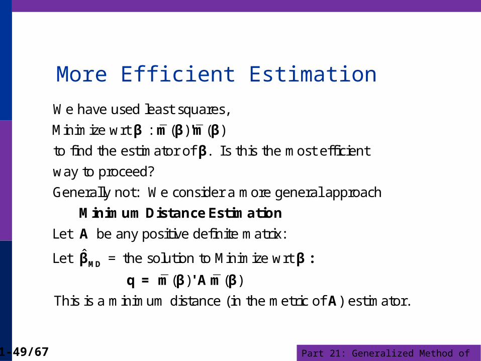
More Efficient Estimation
β m β 'm β
β
Minimum Distance Est
We have used least squares,
Minimize wrt : ( ) ( )
to find the estimator of . Is this the most efficient
way to proceed?
Generally not: We consider a more general approach
MD
imation
A
β β:
q = m β ' A m β
A
Let be any positive definite matrix:
ˆLet = the solution to Minimize wrt
( ) ( )
This is a minimum distance (in the metric of ) estimator.
Part 21: Generalized Method of Moments21-50/67
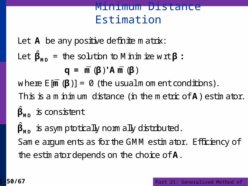
Minimum Distance Estimation
MD
A
β β:
q = m β ' A m β
m β
Let be any positive definite matrix:
ˆLet = the solution to Minimize wrt
( ) ( )
where E[ ( )] = 0 (the usual moment conditions).
This is a minimum distance (in th
MD
MD
A
β
β
A
e metric of ) estimator.
ˆ is consistent
ˆ is asymptotically normally distributed.
Same arguments as for the GMM estimator. Efficiency of
the estimator depends on the choice of .

Part 21: Generalized Method of Moments21-51/67
MDE Estimation: Application
i iy Xβ ε ε X
b β
i i i
i
N units, T observations per unit, T > K
, E[ | ] 0
Consider the following estimation strategy:
(1) OLS country by country, produces N estimators of
(2) How to combine the estimators?
We hav
2
N
b β
b β0
...
b β
β?
1
e 'moment' equation: E
How can I combine the N estimators of
Part 21: Generalized Method of Moments21-52/67
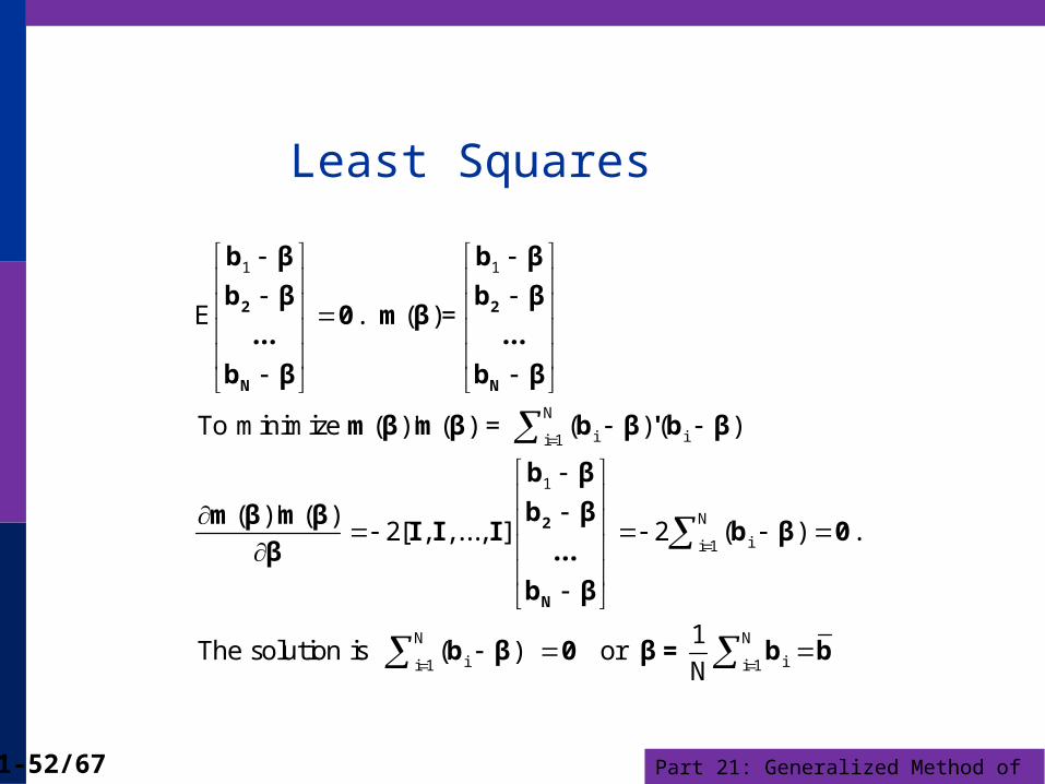
Least Squares
2 2
N N
2
N
b β b β
b β b β0 m β
... ...
b β b β
m β m β b β ' b β
b β
b βm β m βI I I b β 0
...β
b β
b β
1 1
N
i ii 1
1
N
ii 1
i
E . ( )=
To minimize ( )' ( ) = ( ) ( )
( )' ( )2[ , ,..., ] 2 ( ) .
The solution is ( )
0 β= b bN N
ii 1 i 1
1 or
N
Part 21: Generalized Method of Moments21-53/67
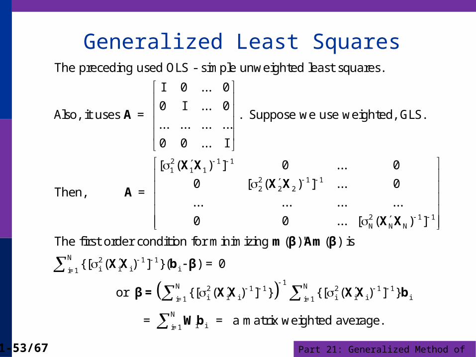
Generalized Least Squares
A
X X
X XA
2 1 11 1 1
22 2 2
The preceding used OLS - simple unweighted least squares.
I 0 ... 0
0 I ... 0Also, it uses = . Suppose we use weighted, GLS.
... ... ... ...
0 0 ... I
[ ( ) ] 0 ... 0
0 [ (Then, =
X X
m β Am β
XX b β
β = XX
1 1
2 1 1N N N
N 2 1 1i i i ii=1
1N 2 1 1 2i i i ii=1
) ] ... 0
... ... ... ...
0 0 ... [ ( ) ]
The first order condition for minimizing ( )' ( ) is
{[ ( ) ] }( ) = 0
or {[ ( ) ] } {[ (
XX b
Wb
N 1 1i i ii=1
N
i ii=1
) ] }
= = a matrix weighted average.

Part 21: Generalized Method of Moments21-54/67
Minimum Distance Estimation
The minimum distance estimator minimizes
( ) ( )
The estimator is
(1) Consistent
(2) Asymptotically normally distributed
(3) Has asymptotic covariance matrix
ˆAsy.Var[ ] [ ( )MD
q = m β ' A m β
β G β 1 1( )] [ ( ) ( )][ ( ) ( )] 'AG β G β 'AVAG β G β 'AG β

Part 21: Generalized Method of Moments21-55/67
Optimal Weighting Matrix
A
A
A
A
is the Weighting Matrix of the minimum distance estimator.
Are some 's better than others? (Yes)
Is there a best choice for ? Yes
The variance of the MDE is minimized when
= {Asy.
generalized method of moments estimator
m β
A V
-1
-1
Var[ ( )]}
This defines the .
=
Part 21: Generalized Method of Moments21-56/67
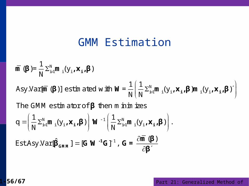
GMM Estimation
i
i i
i i
GM
m β m ,x ,β
m β W m ,x ,β m ,x ,β
β
m ,x ,β 'W m ,x ,β
β
Ni 1 i i
Ni 1 i i i i
N 1 Ni 1 i i i 1 i i
1( )= (y )
N1 1
Asy.Var[ ( )] estimated with = (y ) (y )N N
The GMM estimator of then minimizes
1 1q (y ) (y ) .
N N
ˆEst.Asy.Var[
-1
M
m βG'W G G=
β1 ( )
] [ ] ,

Part 21: Generalized Method of Moments21-57/67
GMM Estimation
i
i
m β m ,x ,β 0
m ,x ,β 'W m ,x
Ni 1 i i
N 1 Ni 1 i i i 1 i i
Exactly identified GMM problems
1When ( ) = (y ) is K equations in
NK unknown parameters (the exactly identified case),
the weighting matrix in
1 1q (y ) (y
N N
i
-1 -1 -1
,β
m β 0
G'W G G WG'1
)
is irrelevant to the solution, since we can set exactly
( ) so q = 0. And, the asymptotic covariance matrix
(estimator) is the product of 3 square matrices and becomes
[ ]
Part 21: Generalized Method of Moments21-58/67
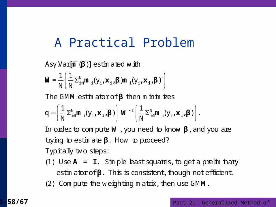
A Practical Problem
Ni 1 i i i i
N 1 Ni 1 i i i 1 i i
Asy.Var[ ( )] estimated with
1 1= (y ) (y )
N N
The GMM estimator of then minimizes
1 1q (y ) (y ) .
N N
In order to compute , you need to know
i i
i i
m β
W m ,x ,β m ,x ,β
β
m ,x ,β 'W m ,x ,β
W , and you are
trying to estimate . How to proceed?
Typically two steps:
(1) Use = Simple least squares, to get a preliminary
estimator of . This is consistent, though not efficient.
(2
β
β
A I.
β
) Compute the weighting matrix, then use GMM.
Part 21: Generalized Method of Moments21-59/67
Inference
Testing hypotheses about the parameters:
Wald test
A counterpart to the likelihood ratio test
Testing the overidentifying restrictions

Part 21: Generalized Method of Moments21-60/67
Testing Hypotheses
m β 'W m β
β
restricted unrestrict
(1) Wald Tests in the usual fashion.
(2) A counterpart to likelihood ratio tests
GMM criterion is q = ( ) ( )
when restrictions are imposed on
q increases.
q q ded chi squared[J]
(The weighting matrix must be the same for both.)

Part 21: Generalized Method of Moments21-61/67
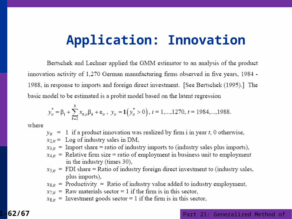
Application: Dynamic Panel Data Model
βxi,t i,t i,t 1 i,t i
(Arellano/Bond/Bover, Journal of Econometrics, 1995)
y y u
Dynamic random effects model for panel data.
Can't use least squares to estimate consistently. Can't use FGLS without
esti
x
xi,1 i i,1
i,1 i i,2
mates of parameters.
Many moment conditions: What is orthogonal to the period 1 disturbance?
E[( u) ] 0 = K orthogonality conditions, K+1 parameters
E[( u) ] 0 = K more orthogonality
xi,1 i i,1
conditions, same K+1 parameters
...
E[( u) ] 0 = K orthogonality conditions, same K+1 parameters
The same variables are orthogonal to the period 2 disturbance.
There are hundreds, sometimes thousands of moment conditions, even for
fairly small models.
Part 21: Generalized Method of Moments21-62/67
Application: Innovation

Part 21: Generalized Method of Moments21-63/67
Application: Innovation

Part 21: Generalized Method of Moments21-64/67
Application: Multivariate Probit Model
5 4 3 2 1
5 1 2 3 4 5
5 - variate Probit Model
y * , y 1[y * 0]
log [{(2 1) , 1,...,5}, ]
Requires 5 dimensional integration of the joint no
i i i i i
it it it it it
i it it i i i i iL y s t ds ds ds ds ds
x x x x x
x
1 1 1
2 2 2
3 3 31
4 4
rmal density. Very hard!
But, E[y | ] ( ).
Orthogonality Conditions: E[{y - ( )}
{y - ( )}
{y - ( )}1
Moment Equations: {y - ( )}
{y - ( )}
it it it
it it it
i i i
i i in
i i ii
i i
n
x x
x x 0
x x
x x
x x
x
4
5 5 5
45 equations in 9 parameters.
{y - ( )}i
i i i
0
x
x x
Part 21: Generalized Method of Moments21-65/67
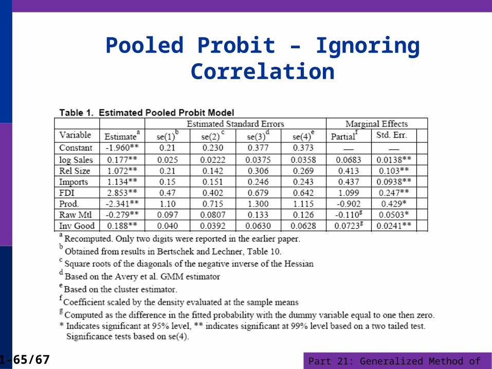
Pooled Probit – Ignoring Correlation
Part 21: Generalized Method of Moments21-66/67
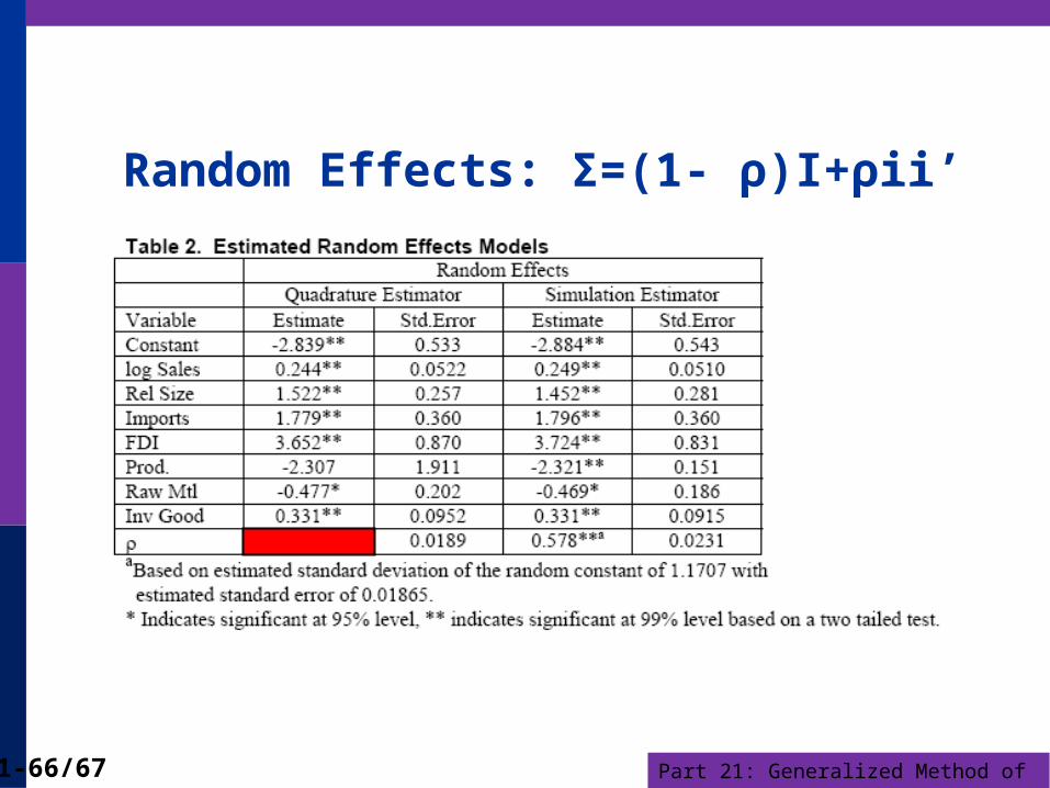
Random Effects: Σ=(1- ρ)I+ρii’
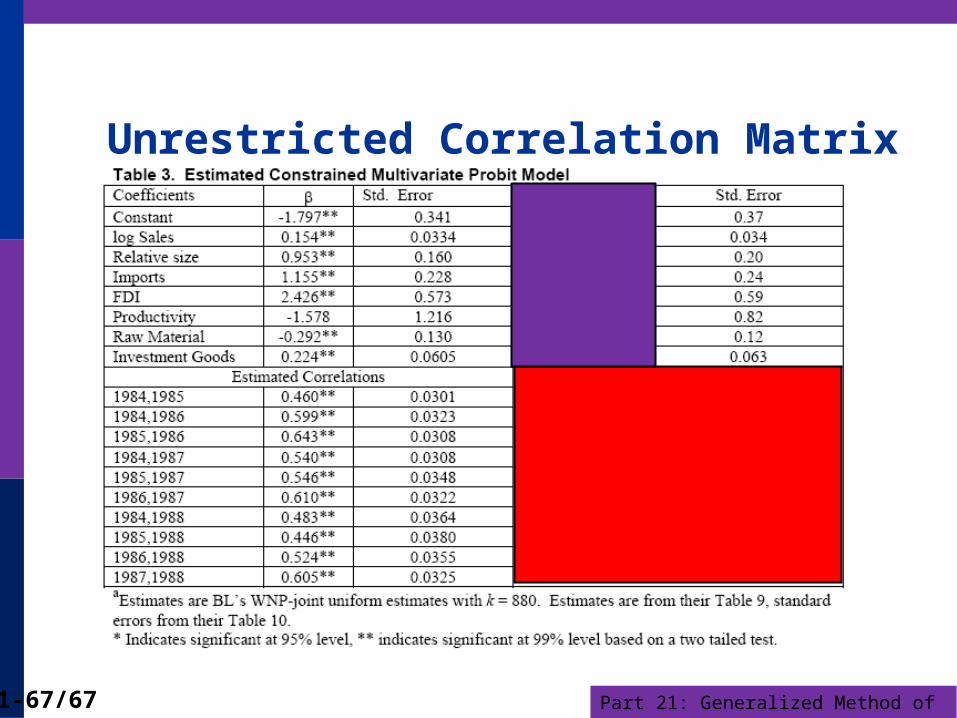
Part 21: Generalized Method of Moments21-67/67
Unrestricted Correlation Matrix
Related Documents


![Part 2: Basic Econometrics [ 1/51] Econometric Analysis of Panel Data William Greene Department of Economics Stern School of Business.](https://static.cupdf.com/doc/110x72/56649d305503460f94a09019/part-2-basic-econometrics-151-econometric-analysis-of-panel-data-william.jpg)
![Part 2A: Basic Econometrics [ 1/75] Econometric Analysis of Panel Data William Greene Department of Economics Stern School of Business.](https://static.cupdf.com/doc/110x72/5697bf731a28abf838c7f4cc/part-2a-basic-econometrics-175-econometric-analysis-of-panel-data-william.jpg)
