Parsing V The LR(1) Table Construction

Welcome message from author
This document is posted to help you gain knowledge. Please leave a comment to let me know what you think about it! Share it to your friends and learn new things together.
Transcript
Parsing V The LR(1) Table Construction
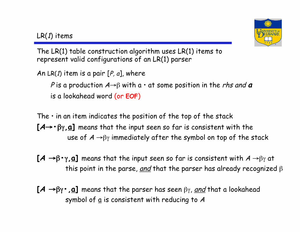
LR(1) items
The LR(1) table construction algorithm uses LR(1) items to represent valid configurations of an LR(1) parser
An LR(1) item is a pair [P, a], where P is a production A→β with a • at some position in the rhs and a is a lookahead word (or EOF)
The • in an item indicates the position of the top of the stack [A→•βγ,a] means that the input seen so far is consistent with the use of A →βγ immediately after the symbol on top of the stack
[A →β•γ,a] means that the input seen so far is consistent with A →βγ at this point in the parse, and that the parser has already recognized β
[A →βγ•,a] means that the parser has seen βγ, and that a lookahead symbol of a is consistent with reducing to A
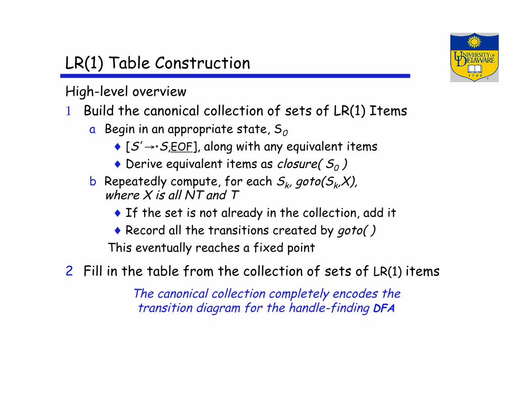
High-level overview 1 Build the canonical collection of sets of LR(1) Items
a Begin in an appropriate state, S0 ♦ [S’ →•S,EOF], along with any equivalent items ♦ Derive equivalent items as closure( S0 )
b Repeatedly compute, for each Sk, goto(Sk,X), where X is all NT and T ♦ If the set is not already in the collection, add it ♦ Record all the transitions created by goto( )
This eventually reaches a fixed point
2 Fill in the table from the collection of sets of LR(1) items The canonical collection completely encodes the transition diagram for the handle-finding DFA
LR(1) Table Construction
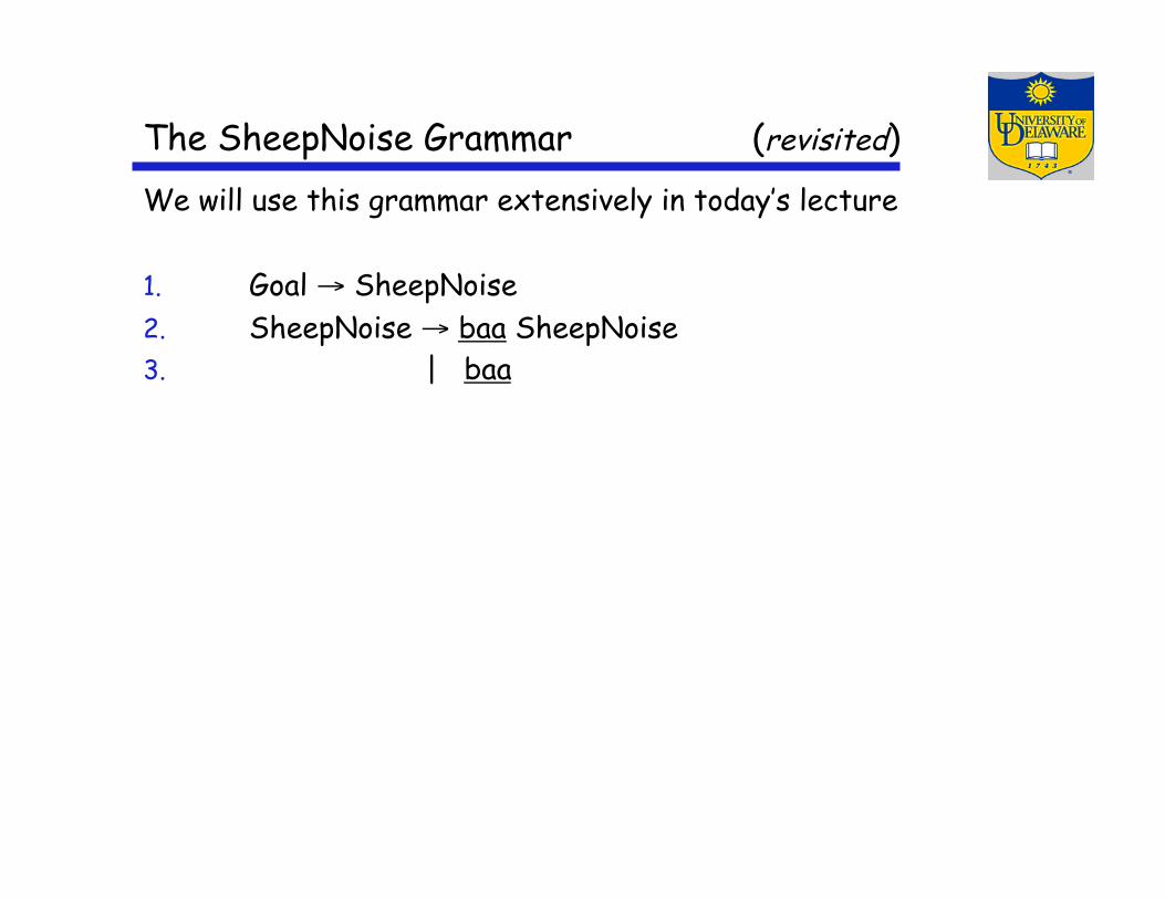
The SheepNoise Grammar (revisited) We will use this grammar extensively in today’s lecture
1. Goal → SheepNoise 2. SheepNoise → baa SheepNoise 3. | baa
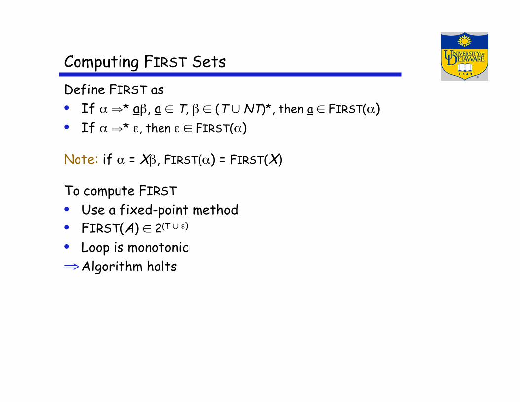
Computing FIRST Sets Define FIRST as • If α ⇒* aβ, a ∈ T, β ∈ (T ∪ NT)*, then a ∈ FIRST(α) • If α ⇒* ε, then ε ∈ FIRST(α)
Note: if α = Xβ, FIRST(α) = FIRST(X)
To compute FIRST • Use a fixed-point method • FIRST(A) ∈ 2(T ∪ ε) • Loop is monotonic ⇒ Algorithm halts
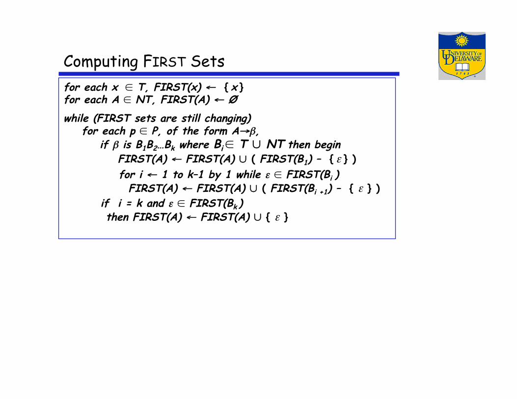
Computing FIRST Sets for each x ∈ T, FIRST(x) ← { x } for each A ∈ NT, FIRST(A) ← Ø while (FIRST sets are still changing) for each p ∈ P, of the form A→β, if β is B1B2…Bk where Bi ∈ T ∪ NT then begin FIRST(A) ← FIRST(A) ∪ ( FIRST(B1) – { ε } )
for i ← 1 to k–1 by 1 while ε ∈ FIRST(Bi ) FIRST(A) ← FIRST(A) ∪ ( FIRST(Bi +1) – { ε } )
if i = k and ε ∈ FIRST(Bk ) then FIRST(A) ← FIRST(A) ∪ { ε }
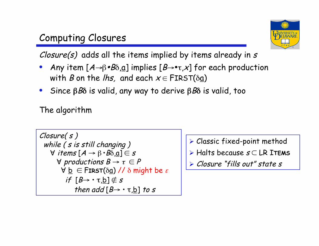
Computing Closures Closure(s) adds all the items implied by items already in s • Any item [A→β•Bδ,a] implies [B→•τ,x] for each production
with B on the lhs, and each x ∈ FIRST(δa) • Since βBδ is valid, any way to derive βBδ is valid, too
The algorithm
Closure( s ) while ( s is still changing ) ∀ items [A → β •Bδ,a] ∈ s ∀ productions B → τ ∈ P ∀ b ∈ FIRST(δa) // δ might be ε if [B→ • τ,b] ∉ s then add [B→ • τ,b] to s
Classic fixed-point method Halts because s ⊂ LR ITEMS Closure “fills out” state s
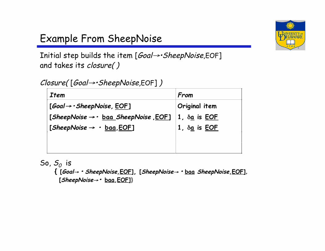
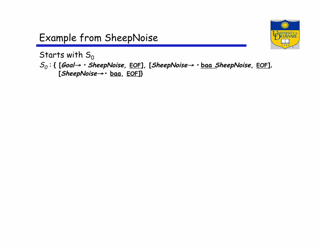
Example From SheepNoise Initial step builds the item [Goal→•SheepNoise,EOF] and takes its closure( )
Closure( [Goal→•SheepNoise,EOF] )
So, S0 is { [Goal→ • SheepNoise,EOF], [SheepNoise→ • baa SheepNoise,EOF], [SheepNoise→• baa,EOF]}
Item From [Goal→•SheepNoise, EOF] Original item
[SheepNoise→• baa SheepNoise ,EOF] 1, δa is EOF [SheepNoise→ • baa,EOF] 1, δa is EOF
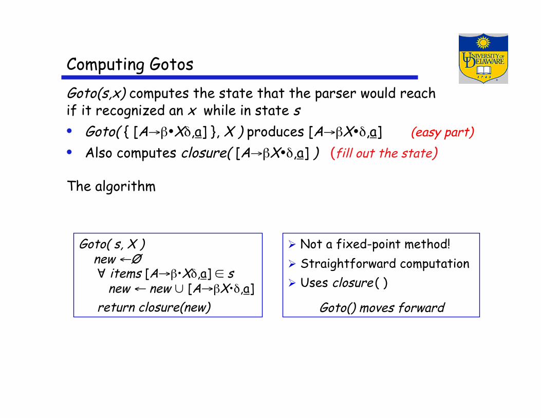
Computing Gotos Goto(s,x) computes the state that the parser would reach if it recognized an x while in state s • Goto( { [A→β•Xδ,a] }, X ) produces [A→βX•δ,a] (easy part) • Also computes closure( [A→βX•δ,a] ) (fill out the state)
The algorithm
Goto( s, X ) new ←Ø ∀ items [A→β•Xδ,a] ∈ s new ← new ∪ [A→βX•δ,a] return closure(new)
Not a fixed-point method! Straightforward computation Uses closure ( )
Goto() moves forward
Example from SheepNoise
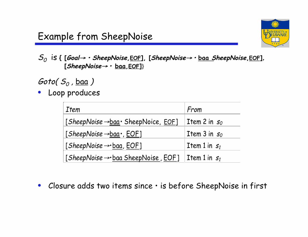
S0 is { [Goal→ • SheepNoise,EOF], [SheepNoise→ • baa SheepNoise,EOF], [SheepNoise→ • baa,EOF]}
Goto( S0 , baa ) • Loop produces
• Closure adds two items since • is before SheepNoise in first
Item From [SheepNoise→baa• SheepNoice, EOF] Item 2 in s0 [SheepNoise→baa•, EOF] Item 3 in s0
[SheepNoise→•baa, EOF] Item 1 in s1
[SheepNoise→•baa SheepNoise , EOF] Item 1 in s1
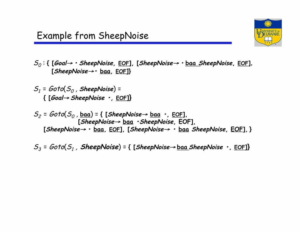
Example from SheepNoise
S0 : { [Goal→ • SheepNoise, EOF], [SheepNoise→ • baa SheepNoise, EOF], [SheepNoise→• baa, EOF]}
S1 = Goto(S0 , SheepNoise) = { [Goal→ SheepNoise •, EOF]}
S2 = Goto(S0 , baa) = { [SheepNoise→ baa •, EOF], [SheepNoise→ baa •SheepNoise, EOF],
[SheepNoise→ • baa, EOF], [SheepNoise→ • baa SheepNoise, EOF], }
S3 = Goto(S1 , SheepNoise) = { [SheepNoise→ baa SheepNoise •, EOF]}
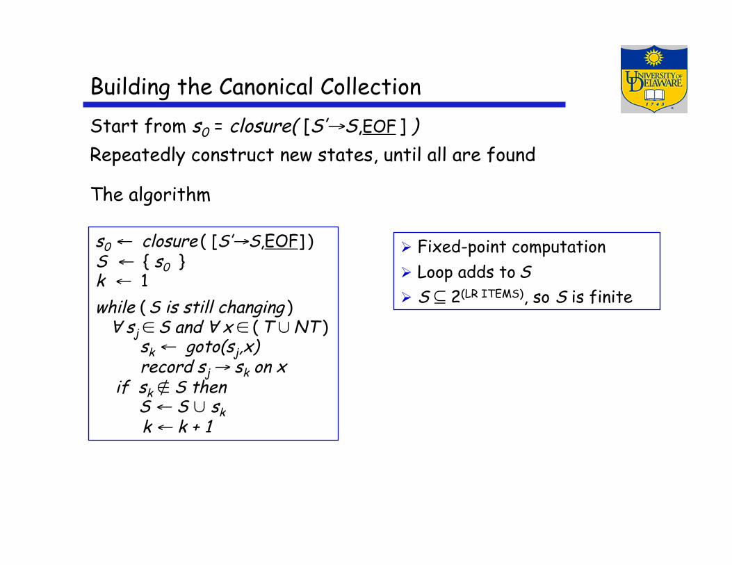
Building the Canonical Collection Start from s0 = closure( [S’→S,EOF ] ) Repeatedly construct new states, until all are found
The algorithm
s0 ← closure ( [S’→S,EOF] ) S ← { s0 } k ← 1 while ( S is still changing ) ∀ sj ∈ S and ∀ x ∈ ( T ∪ NT ) sk ← goto(sj,x) record sj → sk on x if sk ∉ S then
S ← S ∪ sk k ← k + 1
Fixed-point computation Loop adds to S S ⊆ 2(LR ITEMS), so S is finite
Example from SheepNoise Starts with S0 S0 : { [Goal→ • SheepNoise, EOF], [SheepNoise→ • baa SheepNoise, EOF],
[SheepNoise→• baa, EOF]}
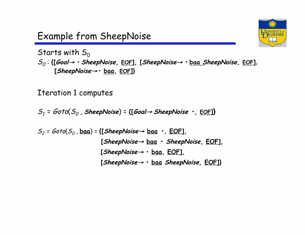
Example from SheepNoise Starts with S0 S0 : {[Goal→ • SheepNoise, EOF], [SheepNoise→ • baa SheepNoise, EOF],
[SheepNoise→• baa, EOF]}
Iteration 1 computes
S1 = Goto(S0 , SheepNoise) = {[Goal→ SheepNoise •, EOF]}
S2 = Goto(S0 , baa) = {[SheepNoise→ baa •, EOF], [SheepNoise→ baa • SheepNoise, EOF],
[SheepNoise→ • baa, EOF], [SheepNoise→ • baa SheepNoise, EOF]}
Example from SheepNoise
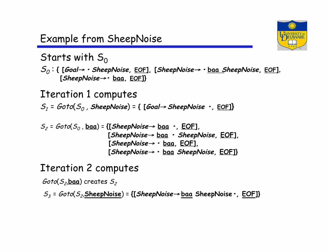
Starts with S0 S0 : { [Goal→ • SheepNoise, EOF], [SheepNoise→ • baa SheepNoise, EOF],
[SheepNoise→• baa, EOF]}
Iteration 1 computes S1 = Goto(S0 , SheepNoise) = { [Goal→ SheepNoise •, EOF]}
S2 = Goto(S0 , baa) = {[SheepNoise→ baa •, EOF], [SheepNoise→ baa • SheepNoise, EOF],
[SheepNoise→ • baa, EOF], [SheepNoise→ • baa SheepNoise, EOF]} Iteration 2 computes Goto(S2,baa) creates S2 S3 = Goto(S2,SheepNoise) = {[SheepNoise→ baa SheepNoise•, EOF]}
Example from SheepNoise
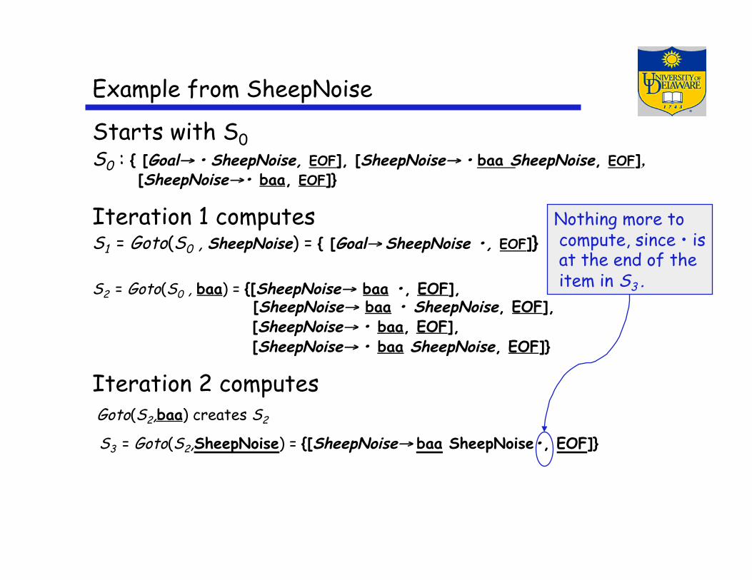
Starts with S0 S0 : { [Goal→ • SheepNoise, EOF], [SheepNoise→ • baa SheepNoise, EOF],
[SheepNoise→• baa, EOF]}
Iteration 1 computes S1 = Goto(S0 , SheepNoise) = { [Goal→ SheepNoise •, EOF]}
S2 = Goto(S0 , baa) = {[SheepNoise→ baa •, EOF], [SheepNoise→ baa • SheepNoise, EOF],
[SheepNoise→ • baa, EOF], [SheepNoise→ • baa SheepNoise, EOF]}
Iteration 2 computes Goto(S2,baa) creates S2 S3 = Goto(S2,SheepNoise) = {[SheepNoise→ baa SheepNoise•, EOF]}
Nothing more to compute, since • is at the end of the item in S3 .
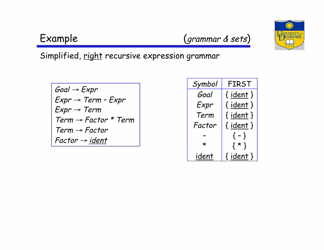
Example (grammar & sets) Simplified, right recursive expression grammar
Goal → Expr Expr → Term – Expr Expr → Term Term → Factor * Term Term → Factor Factor → ident
Symbol FIRSTGoal { ident }Expr { ident }Term { ident }
Factor { ident }– { – }* { * }
ident { ident }
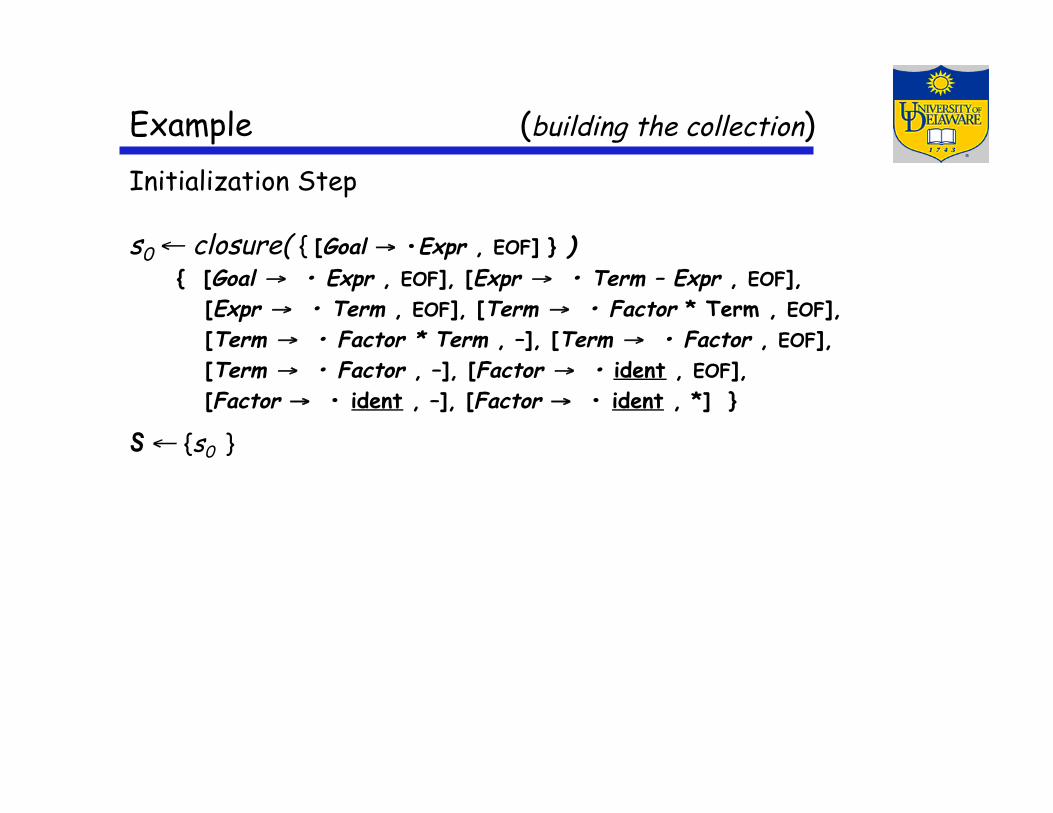
Example (building the collection) Initialization Step
s0 ← closure( { [Goal → •Expr , EOF] } ) { [Goal → • Expr , EOF], [Expr → • Term – Expr , EOF], [Expr → • Term , EOF], [Term → • Factor * Term , EOF], [Term → • Factor * Term , –], [Term → • Factor , EOF], [Term → • Factor , –], [Factor → • ident , EOF], [Factor → • ident , –], [Factor → • ident , *] }
S ← {s0 }
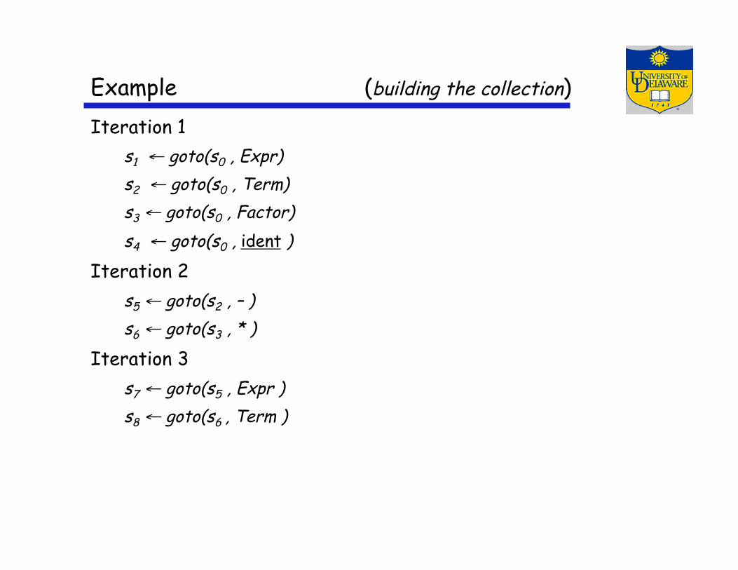
Example (building the collection) Iteration 1
s1 ← goto(s0 , Expr) s2 ← goto(s0 , Term) s3 ← goto(s0 , Factor) s4 ← goto(s0 , ident )
Iteration 2 s5 ← goto(s2 , – ) s6 ← goto(s3 , * )
Iteration 3 s7 ← goto(s5 , Expr ) s8 ← goto(s6 , Term )
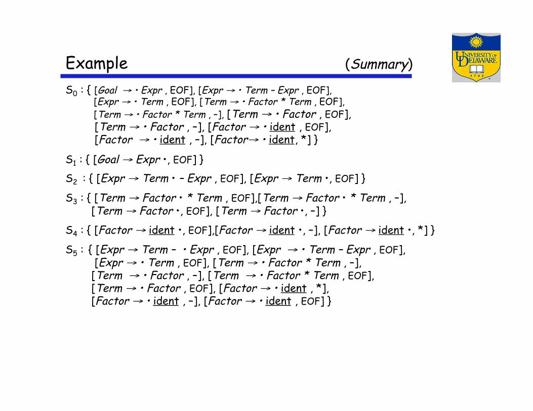
Example (Summary) S0 : { [Goal → • Expr , EOF], [Expr → • Term – Expr , EOF], [Expr → • Term , EOF], [Term → • Factor * Term , EOF], [Term → • Factor * Term , –], [Term → • Factor , EOF], [Term → • Factor , –], [Factor → • ident , EOF], [Factor → • ident , –], [Factor→ • ident, *] } S1 : { [Goal → Expr •, EOF] } S2 : { [Expr → Term • – Expr , EOF], [Expr → Term •, EOF] }
S3 : { [Term → Factor • * Term , EOF],[Term → Factor • * Term , –], [Term → Factor •, EOF], [Term → Factor •, –] }
S4 : { [Factor → ident •, EOF],[Factor → ident •, –], [Factor → ident •, *] }
S5 : { [Expr → Term – • Expr , EOF], [Expr → • Term – Expr , EOF], [Expr → • Term , EOF], [Term → • Factor * Term , –], [Term → • Factor , –], [Term → • Factor * Term , EOF], [Term → • Factor , EOF], [Factor → • ident , *], [Factor → • ident , –], [Factor → • ident , EOF] }
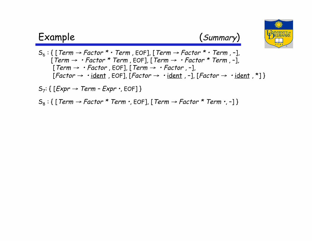
Example (Summary)
S6 : { [Term → Factor * • Term , EOF], [Term → Factor * • Term , –], [Term → • Factor * Term , EOF], [Term → • Factor * Term , –], [Term → • Factor , EOF], [Term → • Factor , –], [Factor → • ident , EOF], [Factor → • ident , –], [Factor → • ident , *] }
S7: { [Expr → Term – Expr •, EOF] }
S8 : { [Term → Factor * Term •, EOF], [Term → Factor * Term •, –] }
Example (Summary)
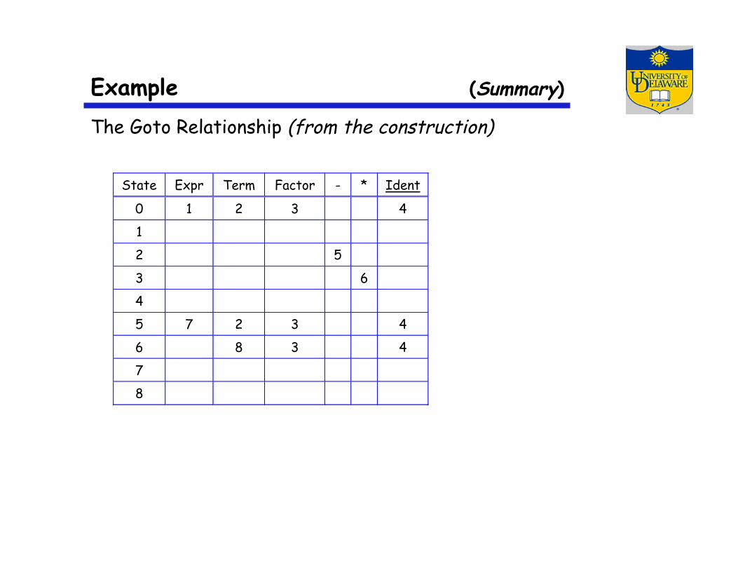
The Goto Relationship (from the construction)
State Expr Term Factor - * Ident
0 1 2 3 4
1
2 5
3 6
4
5 7 2 3 4
6 8 3 4
7
8
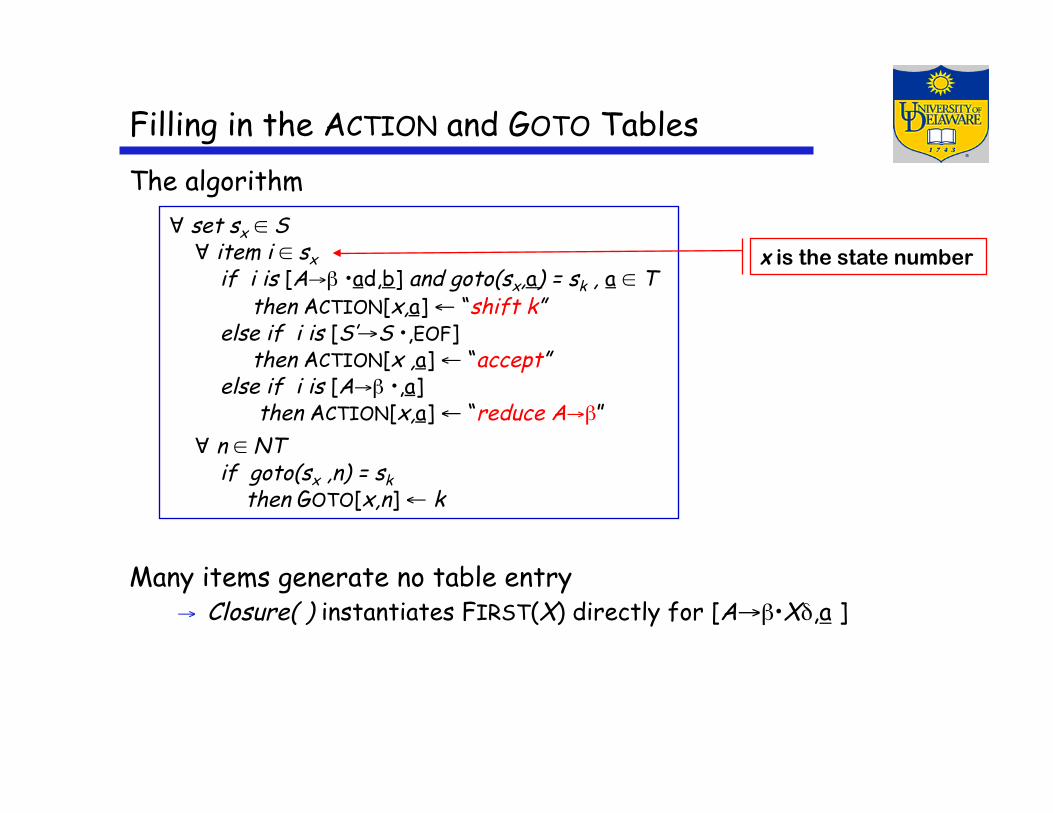
Filling in the ACTION and GOTO Tables The algorithm
Many items generate no table entry → Closure( ) instantiates FIRST(X) directly for [A→β•Xδ,a ]
∀ set sx ∈ S ∀ item i ∈ sx if i is [A→β •ad,b] and goto(sx,a) = sk , a ∈ T then ACTION[x,a] ← “shift k” else if i is [S’→S •,EOF] then ACTION[x ,a] ← “accept” else if i is [A→β •,a] then ACTION[x,a] ← “reduce A→β” ∀ n ∈ NT if goto(sx ,n) = sk then GOTO[x,n] ← k
x is the state number
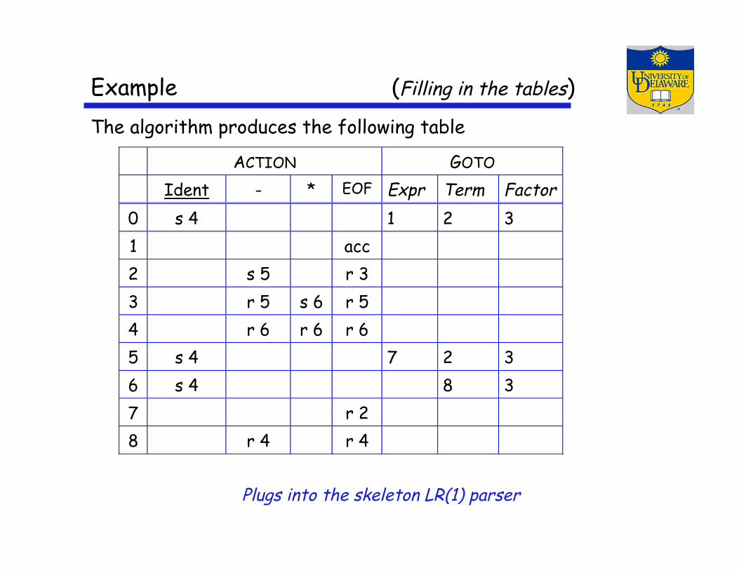
Example (Filling in the tables) The algorithm produces the following table
ACTION GOTO
Ident - * EOF Expr Term Factor0 s 4 1 2 31 acc2 s 5 r 33 r 5 s 6 r 54 r 6 r 6 r 65 s 4 7 2 36 s 4 8 37 r 28 r 4 r 4
Plugs into the skeleton LR(1) parser
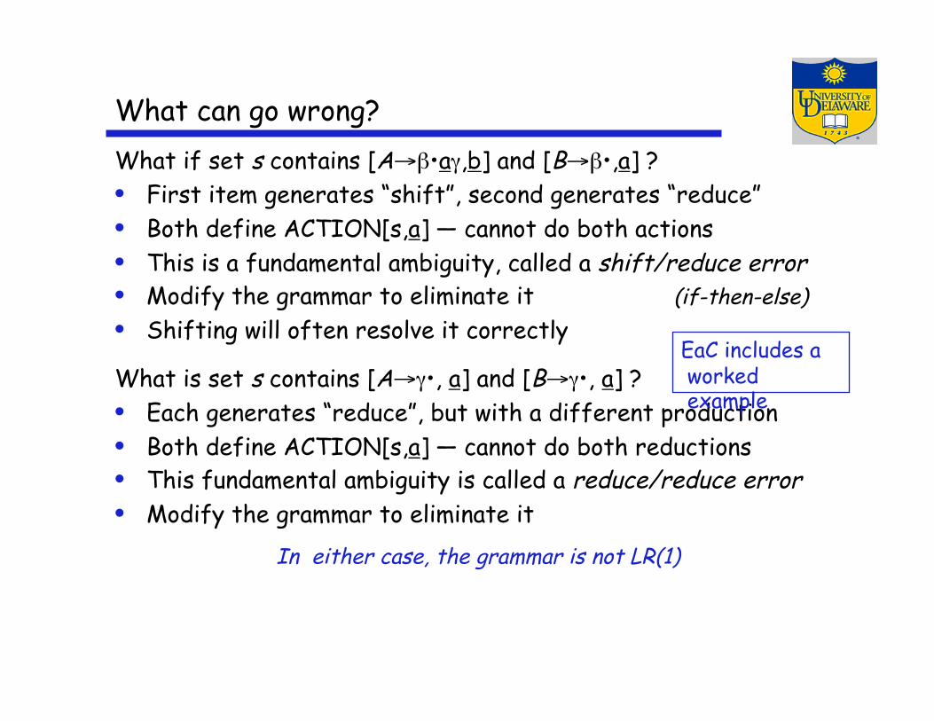
What can go wrong? What if set s contains [A→β•aγ,b] and [B→β•,a] ? • First item generates “shift”, second generates “reduce” • Both define ACTION[s,a] — cannot do both actions • This is a fundamental ambiguity, called a shift/reduce error • Modify the grammar to eliminate it (if-then-else) • Shifting will often resolve it correctly
What is set s contains [A→γ•, a] and [B→γ•, a] ? • Each generates “reduce”, but with a different production • Both define ACTION[s,a] — cannot do both reductions • This fundamental ambiguity is called a reduce/reduce error • Modify the grammar to eliminate it
In either case, the grammar is not LR(1)
EaC includes a worked example
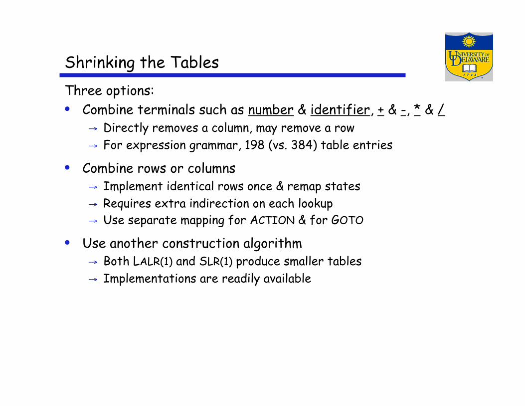
Shrinking the Tables Three options: • Combine terminals such as number & identifier, + & -, * & /
→ Directly removes a column, may remove a row → For expression grammar, 198 (vs. 384) table entries
• Combine rows or columns → Implement identical rows once & remap states → Requires extra indirection on each lookup → Use separate mapping for ACTION & for GOTO
• Use another construction algorithm → Both LALR(1) and SLR(1) produce smaller tables → Implementations are readily available
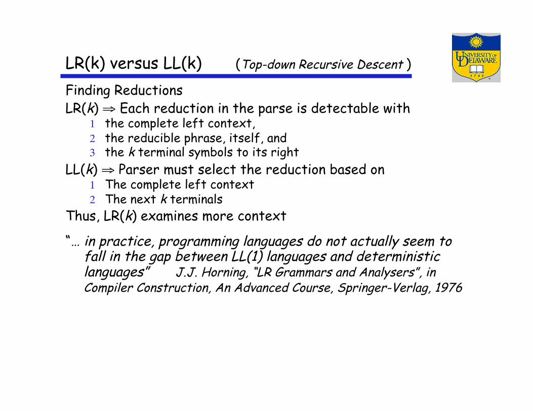
LR(k) versus LL(k) (Top-down Recursive Descent )
Finding Reductions LR(k) ⇒ Each reduction in the parse is detectable with
1 the complete left context, 2 the reducible phrase, itself, and 3 the k terminal symbols to its right
LL(k) ⇒ Parser must select the reduction based on 1 The complete left context 2 The next k terminals
Thus, LR(k) examines more context
“… in practice, programming languages do not actually seem to fall in the gap between LL(1) languages and deterministic languages” J.J. Horning, “LR Grammars and Analysers”, in Compiler Construction, An Advanced Course, Springer-Verlag, 1976
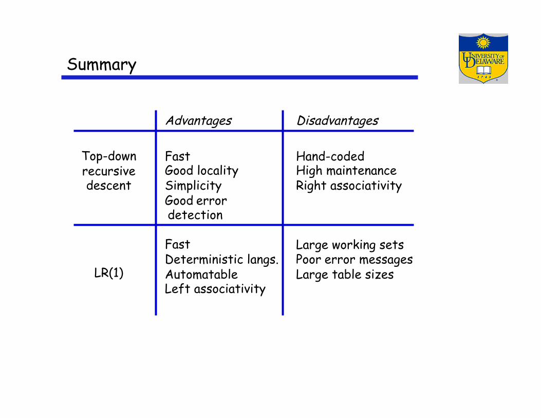
Summary
Advantages
Fast Good locality Simplicity Good error detection
Fast Deterministic langs. Automatable Left associativity
Disadvantages
Hand-coded High maintenance Right associativity
Large working sets Poor error messages Large table sizes
Top-down recursive descent
LR(1)
Related Documents