Parental Responses to Child Support Obligations: Causal ...cle/alluc/RossinSlater_Wust.pdf · Parental Responses to Child Support Obligations: Causal Evidence from Administrative

Page 1

Parental Responses to Child Support Obligations:Causal Evidence from Administrative Data∗

Maya Rossin-Slater†

Miriam Wüst‡

September 3, 2014

Abstract

We leverage non-linearities in Danish child support guidelines together with rich administrativedata to provide causal estimates of parental behavioral responses to child support obligations.We estimate that among families with formal child support agreements, a 1, 000 DKK ($183)increase in a father’s annual obligation is associated with a 573 DKK ($104) increase in hisannual payment. However, we also show that an increase in the obligation reduces the likeli-hood that the father lives with his child, pointing to some substitution between financial andnon-pecuniary investments. Further, we find that larger obligations are associated with highernew-partner fertility among both parents. The maternal fertility response is consistent with apositive income-fertility relationship, while the paternal fertility response may reflect increaseddemand for new offspring as a result of reduced contact with existing children. Finally, we findevidence that some fathers reduce their labor supply to avoid facing higher support obligations.Our findings suggest that government efforts to increase child investments through mandateson parents can be complicated by their behavioral responses to them.

JEL Codes: H4, I1, I3, J1, J2

Keywords: child support, family, divorce, parents, father involvement, fertility, labor supply

∗We thank Paul Bingley, Marianne Bitler, Janet Currie, Olivier Deschênes, Nabanita Datta Gupta, Peter Kuhn,Ilyana Kuziemko, Shelly Lundberg, Mai Heide Ottosen, and Heather Royer as well as seminar participants at UCSanta Barbara, the University of Copenhagen, the SFI annual conference, the ESPE annual conference, the Univer-sity of Wisconsin IRP Summer Research Workshop, and the NBER Summer Institute Children’s Meeting for theirhelpful comments. Rossin-Slater thanks the Danish National Centre for Social Research (SFI) for a research fellowappointment that allows access to the data, and gratefully acknowledges funding from the Regents Junior FacultyFellowship at UC Santa Barbara. All errors are our own.†University of California at Santa Barbara, Department of Economics. Contact e-mail: maya.rossin-

[email protected]‡The Danish National Centre for Social Research (SFI). Contact e-mail: [email protected]

Page 2

1 Introduction

Most modern governments engage in some redistributive policies, whereby income is transferred

from individuals who are taxed to individuals who receive benefits. The donors and recipients

usually do not have any direct connection, and a large body of research has examined the behavioral

responses of these two groups separately. For instance, numerous studies have analyzed the elasticity

of taxable income (see, e.g., Gruber and Saez, 2002; Saez et al., 2012; Piketty and Saez, 2013 for

some surveys), and the fertility and labor supply responses of welfare recipients (see, e.g., Hoynes,

1997; Moffitt, 1998; Schoeni and Blank, 2000; Moffitt, 2002).

However, as a result of the sharp increase in the proportion of children growing up in single-

parent households, a different type of redistributive policy has evolved in the last several decades.1

In the hopes of improving these children’s financial circumstances and shifting the burden of their

support from traditional welfare programs, governments mandate child support payments from

non-custodial parents to the custodial parents and their children.2 As the donors (e.g., fathers)

have a clear connection to the recipients (e.g., mothers and children), the implications of these

policies depend on both the recipients’ and the donors’ preferences and constraints, as well as their

interactions with one another (Weiss and Willis, 1985; Lerman and Sorenson, 2003).

In this paper, we use a new identification strategy and rich administrative data from Denmark

to provide causal estimates of the effects of child support obligations on a wide range of parental

behaviors, thus studying responses among both donors and recipients. To motivate our empirical

analysis, in Section 2, we begin with a conceptual framework that highlights the intertwined nature

of parental incentives and the complexity of their potential responses to child support mandates.

The model demonstrates that child support obligations do not resolve the underlying collective-

goods problem among separated parents (Weiss and Willis, 1985), as custodial parents have full

allocative power over how to spend the non-custodial parents’ payments. As a consequence, non-

custodial parents may view their obligations as taxes, which may not always benefit their children.

Moreover, the framework shows that when the child support obligation is linked to the custody

arrangement (e.g., if the child support mandate is different depending on whether the parents share1In the U.S., 9 percent of children under age 18 lived with only one biological parent in the household in 1960,

while over 26 percent do today. Many Western European countries have similar rates—for example, about 22 percentof British children, 18 percent of Danish children, and 15 percent of German children live with only one parent. Datafor the European countries are from EU Community Statistics on Income and Living Conditions, 2007. Data for U.S.are from the 1960 Decennial Census and the 2013 Current Population Survey.

2Children in single-mother households are disproportionately low-income. In the U.S., children in single-motherhouseholds are twice as likely to live in poverty relative to the average child. In Denmark, children in single-motherhouseholds are three times more likely to live in poverty relative to the average child. For more information on childpoverty rates in Europe, see: http://www.unicef-irc.org/publications/pdf/rc10_eng.pdf.

1

Page 3

custody), it may affect parental decisions about child custody, as well as other voluntary and non-

pecuniary investments and contact with children. These decisions may in turn have downstream

effects on a variety of other parental behaviors, including family formation with new partners and

labor market activities. The implications for child well-being and public spending are both complex

and theoretically ambiguous.

The existing evidence on the causal effects of child support mandates is limited. Researchers

are faced with two main challenges. First, child support obligations are not randomly assigned,

making it difficult to disentangle their causal effects from the possible influences of other (unobserv-

able) differences between families. The second challenge stems from a substantial data constraint,

especially in the United States, where most of the existing work has been set (see Garfinkel et al.,

1998; Del Boca, 2003; Lerman and Sorenson, 2003; Cancian et al., 2011 for some surveys). Data

sets typically measure outcomes for individuals in a given household, making it impossible to link

children to their non-custodial parents. Additionally, because many of the existing studies use

survey data such as the Current Population Survey, this literature relies heavily on self-reported

income measures, which may be missing or inaccurate for a significant fraction of respondents

(Weinberg, 2006). As such, researchers are unable to precisely identify child support obligations

(which are based on parental income), and to our knowledge, no studies have exploited variation

in child support guidelines across individuals with different incomes.

Our paper addresses these challenges by proposing a new identification strategy that exploits

non-linearities in Danish child support guidelines, which assign non-custodial parents different

obligations according to their incomes, numbers of children, and years of separation. As described in

more detail in Section 3, every year, all non-custodial parents under formal child support agreements

are required to pay the same base amount per child. Non-custodial parents with incomes above

certain thresholds must also pay additional percentages of the base amount, which range between 25

and 300 percent, depending on the location of the threshold. The locations of the income thresholds

vary by the number of children and by year. Additionally, the base amount has increased above

the rate of inflation in every year during our analysis time frame.

We use this variation together with administrative data on the universe of Danish children linked

to their parents regardless of their residence status and with precise information on parental income,

as described in detail in Section 4. We are thus able to comprehensively analyze the effects of child

support obligations on fathers’ payments to children, fathers’ likelihood of co-residence with their

children, as well as both parents’ post-separation family formation and labor market behavior, as

2

Page 4

we explain in Section 5.3 Our analysis uses data on all parents who divorce, separate, or have a child

outside marriage or cohabitation over 1999-2008. For each father and in each year post-separation

observed in the data, we calculate the annual child support obligation he should face based on his

income and number of children measured in the year of separation. Put differently, these calculated

obligations are based only on variation in the government-mandated guidelines, and do not take

into account any changes to the father’s income or number of children after separation, as such

changes may reflect endogenous responses. To identify the causal effects of these obligations, we

rely on an assumption that there are no omitted variables that systematically covary with the child

support guidelines and differentially affect fathers across income levels, number of children, and

years of separation. In support of this assumption, we: (1) provide evidence that our calculated

obligations are uncorrelated with a variety of parental characteristics that are not used in setting

them, and (2) show that anticipated child support obligations are uncorrelated with selection into

divorce, separation, or out-of-wedlock/cohabitation childbearing in the first place.

Our results point to important parental behavioral responses to the child support mandates,

as detailed in Section 6. First, we show that child support mandates are moderately effective at

increasing financial transfers from non-custodial fathers to children. Among all separated parents,

a 1, 000DKK ($183) increase in a father’s average annual child support obligation is associated with

a 430DKK ($78) increase in his average annual payment. Scaling by a formal agreement rate of 75

percent (Skinner et al., 2007) implies a treatment-on-the-treated (TOT) relationship of a 573DKK

($104) increase in payments for every 1, 000DKK increase in obligations.

Next, we examine how the child support obligation affects the likelihood that a father ever

resides with his child post-separation. In Denmark, parents who share equally in physical custody

are not mandated to make child support payments; hence, a higher obligation may increase the

incentive for the father to live with his child at least part of the time so to avoid making a larger

payment. However, mothers, who have substantial say in custody decisions, have the opposite

incentive to refuse to share custody and instead receive the higher payment. Moreover, fathers may

consider financial transfers as substitutes for other forms of non-pecuniary investments and contact

with children, which would also lead to a negative relationship between child support obligations

and paternal physical custody rates. We find that these latter forces dominate in our data—an3Our analysis focuses on studying the effects of fathers’ child support obligations because they are much more

likely than mothers to become the non-custodial parents in case of separation. For example, according to StatisticsDenmark, in 2010, about 26 percent of children lived with only one biological parent. Out of them, 23 percent livedwith only their mothers or their mothers and their partners, while 3 percent lived with only their fathers or theirfathers and their partners. While we observe information on whether the father lives with his child post-separation,we purposely do not drop these fathers since we show that residence with the child is an outcome that can be affectedby the child support obligation.

3

Page 5

additional 1, 000DKK in a father’s average annual child support obligation leads to an 1.8 percent

reduction in the likelihood that he resides with his child in at least one year post-separation.

We also analyze parental fertility responses. We find that a 1, 000DKK increase in the father’s

average annual child support obligation leads to a 2.7 percent increase in the likelihood that the

mother has an additional child post-separation, consistent with a positive income-fertility relation-

ship documented in other studies analyzing child tax and welfare benefits in Western Europe and

Canada (Laroque and Salanié, 2008; Brewer et al., 2012; Milligan, 2005).

Fathers face unique fertility incentives because the locations of the income thresholds in the

Danish child support guidelines are increasing in the number of biological children, and because

the per-child obligation is set according to the father’s total number of children (including those

within subsequent unions) but only applies to his non-custodial children. Consequently, some

fathers can reduce their obligations to their non-custodial children by having more children within

unions with new partners. Additionally, our result on father-child co-residence suggests that, for

all fathers, an increase in the obligation may lead to less attachment to existing children and more

time available to invest in new offspring. We find evidence consistent with these positive fertility

incentives: a 1, 000DKK increase in a father’s average annual obligation increases his likelihood of

having a subsequent child by 3.1 percent. This effect is driven by fathers having children while

married to or cohabiting with new partners, and by fathers who do not reside with their older

children.

Finally, we find that fathers change their labor market behavior in response to child support

obligations, while mothers do not. Overall, a 1, 000DKK increase in a father’s average annual child

support obligation reduces his labor force participation by 0.15 percent. This average treatment

effect masks important heterogeneity, however. Fathers with separation year incomes below the

first guideline threshold, who must all pay the same lump-sum base amount, actually increase their

labor supply. In contrast, fathers with separation year incomes above the first threshold—who must

make supplemental payments and thus face a competing incentive to reduce their earnings—are the

ones driving the decline in labor force participation. This labor supply decline reflects transitions

into disability insurance and discretionary early retirement programs. As such, we provide novel

support for the relationship between the relative value of labor market participation and the take-

up of these programs, which has been previously documented both in Scandinavia (Bratsberg et al.,

2010; Bingley et al., 2011) and in the U.S. (Black et al., 2002; Autor and Duggan, 2003).

As we discuss further in Section 7, our findings suggest that government interventions into

families with divorced and unmarried parents result in important parental behavioral changes that

4

Page 6

can distort their intended impacts on child investment levels, public spending, and overall child

well-being. While fathers respond to child support orders with increased financial transfers to

their children, they also reduce their contact with them. Moreover, the increases in both parents’

subsequent fertility rates point to possible reductions in the allocation of resources toward the

existing children whom child support guidelines are meant to help. Finally, the decreases in paternal

labor supply among higher-income fathers demonstrate the market distortions generated by the

“tax-like” nature of child support mandates. Our results suggest that although child support

mandates may shift some of the cost of single-mother household support from welfare programs to

the non-custodial fathers, they also pass part of this cost on to other government programs such

as disability insurance and early retirement.

In sum, our results highlight the role of parental agency in family resource allocation, and

suggest that government efforts to increase child investment levels through mandates on parents

can be complicated by their behavioral responses to them.

2 How Might Child Support Obligations Affect Parental Behaviors?

This section presents a general framework for understanding the channels through which non-

custodial parents’ child support obligations could affect parental behaviors after separation.4 This

framework draws on several existing models of interaction within non-intact families (e.g., Weiss and

Willis, 1985; Del Boca and Flinn, 1995; Willis, 1999; Flinn, 2000; Del Boca and Ribero, 2003; Roff

and Lugo-Gil, 2012). As noted above, throughout this paper, we treat fathers as the non-custodial

parents and mothers as the custodial parents.

2.1 Conceptual Framework

Consider a set of separated parents with one child between them, where mothers are denoted by

subscript m and fathers are denoted by subscript f . Each parent obtains utility from child quality,4Child support orders, which, in theory, make separation and family formation more costly for non-custodial

fathers and increase custodial mothers’ bargaining power, may also influence the rates of divorce and separationamong parents who are still together, as well as the rates of childbearing outside marriage and cohabitation amongmen and women who are not yet parents (Brown and Flinn, 2011). Other policies, such as unilateral divorce lawsand joint custody reforms, which aim to affect the outcomes of families with divorced and unmarried parents, havebeen shown to also impact divorce and marriage rates (Stevenson and Wolfers, 2006; Wolfers, 2006; Halla, 2013).Such effects can complicate the study of outcomes among separated parents because of bias due to the treatment (inour setting, the child support order) being correlated with selection in or out of the sample of analysis. However, thisissue is not empirically relevant in our context. As discussed in detail in Section 5, we find no relationship betweenchild support obligations and the likelihood of parental separation in our data.

5

Page 7

Q, their own private adult consumption, C, and their leisure time, L.5 Utility from child quality

is comprised of two components: Q0 (current child quality), Q1 (child quality from a possible

subsequent child born within a new union). For simplicity, we do not explicitly model future

children born outside marriage/cohabitation; however, we discuss how incorporating this decision

into the model would affect the main conclusions below. For each parent i ∈ {m, f}, denote the

number of subsequent children by ni, where ni can take on integer values {0, 1, 2, . . .}.

Additionally, assume that child quality is a function of two types of investments: financial,

F , and time, K. Denote the financial and time investments in the current child by F 0 and K0,

respectively. For mothers’ subsequent children, financial and time investments are F 1m and K1

m,

respectively; for fathers’ subsequent children, financial and time investments are F 1f and K1

f , re-

spectively.

Thus, in terms of time allocation, each parent must divide his/her time between work in the

labor market (denoted by H), time investments into children, and leisure. Each parent i ∈ {m, f}

earns wage wi in the labor market, and total time available is denoted by T .

We assume that the separated parents do not bargain cooperatively and instead face a static

Stackelberg game.6 In this setting, the non-custodial father can make two types of transfers to the

custodial mother: a financial transfer, s, and a time transfer, t. The custodial mother chooses how

to allocate these transfers. Intuitively, we can think of the time transfer as the amount of extra

time freed up for the mother as a result of the father offering to spend time with the child.

For subsequent children, we assume that the parents expect to bargain cooperatively with new

partners. Each parent i expects to be responsible for fraction λFi of the total financial investment

and fraction λKi of the total time investment per subsequent child born.5Note that our framework differs from the model in Neal (2004), which assumes that “absent fathers do not

enjoy any consumption gains from having children”. We instead follow Willis (1999) and Flinn (2000) (among manyothers) by assuming that non-custodial fathers in fact obtain utility from child quality. This assumption is arguablymore realistic in our setting, where an estimated 20 percent of Danish children with divorced or separated parentshave fathers who share in their physical custody (Bjarnason and Arnarsson, 2011), and another 45 percent havenon-custodial fathers who visit with them at least every other weekend (Kampmann and Nielsen, 2004).

6The non-cooperation assumption is common in the literature on non-intact families (e.g., Weiss and Willis, 1985;Del Boca and Flinn, 1995; Willis, 1999; Roff and Lugo-Gil, 2012). In an important contribution, Flinn (2000)instead develops a model where separated parents can choose between cooperative and non-cooperative equilibria,and where institutions (e.g., judges determining child support or custody settlements) are modeled as coordinationdevices. Such a model is useful for generating predictions about the impacts of changes to institutional enforcementcapabilities. For example, a key result of the model is that when institutions can perfectly enforce compliance withchild support orders, the custodial parent loses the incentive to engage in cooperative behavior; for a large set ofparental preferences, perfect child support enforcement can thus lead to lower child investments relative to imperfectenforcement. In our case, the empirical analysis uses variation in child support order amounts, rather than in thedegree of institutional enforcement (in fact, enforcement does not change throughout our sample time frame). Assuch, we do not take this approach, and instead assume perfect complicance with child support orders (see below).

6

Page 8

More concretely, ∀i ∈ {m, f} parental utility is represented by the following function:

U

(Q0, Q1

i , ni, Ci, Li

)= βiUc

(Q0(F 0,K0), ni ∗Q1(F 1

i ,K1i ))

+ (1− βi)Ua(Ci, Li

)

where Uc(·) represents utility from children, Ua(·) represents utility from adult activities, and βi,

0 < βi < 1, represents the weight each parent places on his/her preferences toward children relative

to other adult consumption goods.7

The mother chooses the optimal current and subsequent child investments, the number of

subsequent children she will have, and her own adult consumption and leisure, conditional on the

father’s transfers:8

maxF 0,K0,nm,F 1

m,K1m,Cm,Lm

βmUc

(Q0(F 0,K0), nm ∗Q1(F 1

m,K1m))

+ (1− βm)Ua(Cm, Lm

)

s.t. F 0 + nmλFmF

1m + Cm = wm

(T − Lm −K0 + t− nmλKmK1

m

)+ s

The father then maximizes his indirect utility function, taking into account the maternal optimal

response functions for current child investments, F 0(s, t)∗ and K0(s, t)∗. He chooses his optimal

financial and time transfers for the current child, the number of subsequent children he will have,

his investments into subsequent children, his private adult consumption, and his time spent in

leisure. Additionally, we assume that for the current child, the father is subject to a child support

mandate, R, which depends on his earned income, his number of children, and his time transfer,

and is defined further below. The father thus solves the following problem:

maxs,t,nf ,Lf ,F

1f,K1

f

{βfUc

(Q0(F 0(s, t)∗,K0(s, t)∗

), nf ∗Q1(F 1

f ,K1f

))

+(1− βf )Ua(wf (T − Lf − t− nfλKf K1

f )− s− nfλFf F 1f , Lf

)}s.t. s ≥ R(wfHf , nf , t)

The child support obligation for the current child, R(wfHf , nf , t), is set according to a formula

that depends on the father’s earned income, wfHf , his total number of biological children (nf +1),

and his time transfer, t, in a way similar to the actual Danish child support guidelines that we

study. In particular,7While we do not make any assumptions about a particular functional form of the utility function in this discussion,

we note that the utility function in this framework must allow for corner solutions as ni is allowed to be set to zero.More formally, it must be that limx→0 U ′(x) 6=∞.

8Prices of consumption goods are normalized to 1 for simplicity.

7

Page 9

R(wfHf , nf , t) =

ξ if wfHf ≤ Y nf

and t ≤ t

ξ + τ if wfHf > Y nfand t ≤ t

0 if t > t

for some ξ > 0, τ > 0, and t > 0. Additionally, Y nf> 0 and is strictly increasing in nf . In other

words, the guidelines are set such that fathers must pay a base amount, ξ, and fathers with incomes

above some threshold, Y nf, face an additional obligation of τ . The location of Y nf

is increasing

with the father’s subsequent number of children, nf . The child support constraint is removed once

fathers make high enough time transfers, t. For example, in our context, fathers who share in

physical custody of their children do not need to pay child support.

Denote the father’s optimal financial transfer by:

s∗ = max(sunc, R(·)

)

where sunc is the (unconstrained) solution to the father’s optimization problem if the child support

mandate constraint is not binding.9

2.2 Possible Effects on Parental Behaviors

Consider two order schemes: R1(wfHf , nf , t) and R2(wfHf , nf , t), with ξ2 > ξ1 and τ2 > τ1. What

happens to parental behaviors when we increase the child support obligation from R1 to R2? Our

model highlights the theoretical ambiguity of this question with regard to the following parental

behaviors:

Fathers’ Financial Transfers Consider three possible cases that depend on what fathers’ fi-

nancial transfers would have been in the absence of government intervention:

First, if sunc ≥ R2, the father optimally transfers as much or more than what is mandated

under the higher order, R2. This father will not alter s∗ in response to a switch from the lower to

the higher order.9As noted, we assume perfect compliance with child support mandates and do not model the compliance decision.

This decision is modeled explicitly through an incorporation of a cost associated with non-compliance in Del Bocaand Flinn (1995) and Flinn (2000). Modeling the compliance decision is important in a setting where the degreeof institutional enforcement changes and child support obligations are set endogenously (e.g., by judges). In ourcase, enforcement is stable over the analysis time frame, and we argue that our variation in child support orders ispolicy-driven and exogenous.

8

Page 10

Second, if R1 < sunc < R2, then the father would optimally pay more than the lower order, R1,

but less than the higher order, R2. When faced with a change from R1 to R2, it may be optimal

for the father to increase s∗ from sunc to R2. The magnitude of this increase is strictly less than

the difference between the two order schemes, R2−R1. However, as discussed further below, some

fathers may also respond by having more children or lowering their labor supply so to reduce their

R2 obligations from ξ2 + τ2 to ξ2. If ξ2 < sunc < ξ2 + τ2, then there may be a decrease in s∗ from

sunc to ξ2.

Third, if sunc ≤ R1, then the father would optimally pay less than the lower order. There are

two possibilites for these fathers as well. Some fathers may increase s∗ exactly from R1 to R2 (either

from ξ1 to ξ2 or from ξ1 + τ1 to ξ2 + τ2). However, as before, if some fathers respond by having

more children or lowering their labor supply, s∗ may instead change from ξ1 + τ1 to ξ2, which may

reflect either an increase or a decrease in optimal payments, depending on whether ξ2 is smaller or

larger than ξ1 + τ1.

Thus, while increases in child support orders are predicted to increase some fathers’ financial

transfers to their children, this relationship is complicated by other paternal behaviors, and may

not be one-for-one on average. Some fathers may just substitute for non-mandated transfers that

they would have made in the absence of government intervention. Additionally, fertility and labor

supply responses may even lead to a perverse relationship between child support mandates and

actual payments.

Fathers’ Time Investments There are two opposing forces on fathers’ time investments. On

the one hand, since fathers who make high enough time transfers do not face the child support

mandate, a higher order may lead to an increase in t∗ as the father can forego a larger financial

cost by being above t.

On the other hand, the higher order increases the maternal incentive to actually receive the

higher mandated financial transfer by ensuring (via her optimal response functions) that the father’s

time transfer does not exceed t. In our setting, when the father is faced with the higher order, the

mother has a greater incentive to make sure that the father does not share in physical custody.10

Moreover, since child quality is a function of both financial and time investments, and since higher10In practice, parents can either agree on a custody arrangement informally or they can go to the court if they

are unable to reach an agreement. Hence, if the mother refuses to share physical custody, the father can in principletake the issue to court. However, prior to a reform in October 2007, which made joint legal custody the defaultdetermination (and hence made joint physical custody more likely as well), courts were likely to rule in favor ofmaternal sole custody. Thus, it is reasonable to assume that, during our sample time frame of 1999-2008, mothershad substantial influence over the custody decision.

9

Page 11

orders increase financial investments, F , there may be additional downward pressure on paternal

optimal time transfers, t∗, due to properties of the child quality function (i.e., if financial and time

investments are at all substitutes).

Both Parents’ New Family Formation Fathers face complex fertility incentives. First, for

fathers with incomes below the threshold, Y nf, a higher order represents a negative income effect,

which may decrease subsequent fertility. However, since the income threshold is increasing in the

number of subsequent children, and since the father is only mandated to make financial transfers to

his one existing non-custodial child, some (higher-income) fathers have an incentive to have more

children so to reduce their child support obligation from ξ + τ to ξ. Additionally, for fathers at all

income levels, higher orders may lead to less time spent with existing children, t∗, freeing up time

available to invest in future children.

For mothers, consider the case where higher orders increase fathers’ financial transfers. For

them, higher orders constitute larger positive income effects, resulting in greater investments in

current children as well as greater demand for subsequent children. Mothers also face an opposite

incentive to lower subsequent fertility because their time available to invest in subsequent children

may be lower as a result of a reduction in the paternal time transfer.

Moreover, although we do not model this explicitly, there are different incentives for mothers’

and fathers’ subsequent fertility outside marriage and cohabitation. In particular, although a father

may lower his per-child obligation by having more children out-of-wedlock/cohabitation (since the

income threshold is increasing in his total number of children), fertility within unions is relatively

less costly as he is only subject to child support mandate for his out-of-union children. By contrast,

a mother may have larger incentives for childbearing outside unions because the receipt of a higher

payment for her existing child may increase her expectation of child support transfers associated

with subsequent offspring from new partners.11

Both Parents’ Labor Market Behavior Fathers face opposing labor supply incentives. For

a father with earnings below the threshold, Y nf, the child support order is a flat negative income

shock in the amount of ξ. This shock is predicted to reduce demand for leisure and increase labor

supply. In contrast, a father with an income above the threshold faces a type of tax on earnings.

This higher-income father has an incentive to lower his labor supply in order to reduce his income11Note that all of these fertility responses for fathers and mothers are relevant insofar as we hold the fertility

responses of the other parents constant. As these parents are all arguably in the same matching market post-separation, the net effects on overall parental fertility rates also depend on the numbers of men and women and theirrelative bargaining powers.

10

Page 12

and avoid paying the additional τ amount.

For a mother, again consider the case where a higher order increases the father’s financial

transfer. The child support order is then a positive income shock that is not dependent on her own

earned income. As such, we may expect an increase in maternal demand for leisure and therefore a

reduction in her labor supply. Additionally, maternal labor supply may also be affected by possible

changes to her time available to work due to impacts on the father’s time transfer.

2.3 Existing Evidence on Child Support

There are two strands of existing literature on issues related to child support, both focused on the

U.S. setting. One strand has used a structural model approach to directly estimate parameters of

utility functions among separated parents (see, e.g., Del Boca and Flinn, 1995; Flinn, 2000; Del Boca

and Ribero, 2003; Brown and Flinn, 2011; Roff and Lugo-Gil, 2012; Tartari, 2014). This approach

is also useful for generating predictions about the impacts of various policy counterfactuals (e.g.,

perfect institutional enforcement of child support orders versus weak enforcement). As with all

such structural estimations, however, functional form assumptions and concerns about endogeneity

present some limitations.

We take a complementary approach by using quasi-exogenous variation in an existing policy

(namely, the Danish child support guidelines) and studying the reduced-form impacts of child

support obligations on a wide range of parental behaviors. While our results cannot directly speak

to parental preferences or overall welfare, our analysis instead focuses on producing causal estimates.

We thus more directly contribute to the other strand of existing literature on child support,

which uses variation across U.S. states in child support enforcement spending or the implementation

of specific policies (such as automatic wage withholding and license revocation for non-payment) to

identify their effects. Several such studies have shown that child support enforcement policies and

spending are correlated with higher child support payments (Sorensen and Halpern, 1999; Freeman

and Waldfogel, 2001; Sorensen and Olivier, 2002; Cancian et al., 2007), and have varied effects

on non-mandated forms of involvement (Nepomnyaschy, 2007; Nepomnyaschy and Garfinkel, 2010;

Gunter, 2013).12 The evidence on paternal labor supply is also mixed: Freeman and Waldfogel

(1998) find no correlation between child support enforcement and fathers’ work behavior, while

Holzer et al. (2005) and Cancian et al. (2013) show a negative relationship between child support12In particular, Nepomnyaschy (2007) finds fathers who pay more child support increase contact with their children

(i.e., formal payments and contact are complements); Nepomnyaschy and Garfinkel (2010) find evidence of substitu-tion between formal and voluntary payments; Gunter (2013) shows that formal payments and in-kind transfers maybe substitutes as well.

11

Page 13

mandates and paternal formal labor supply. With regard to family formation, to the best of our

knowledge, no previous work has examined subsequent fertility patterns of mothers and fathers

who have already separated. However, there is evidence that greater child support enforcement is

negatively correlated with overall non-marital fertility rates, possibly implying that a deterrence

effect on men may dominate the opposite effect on women (Case, 1998; Huang, 2002; Plotnick et al.,

2004; Aizer and McLanahan, 2006).13

On the whole, the existing literature cannot yet paint a complete picture of the implications of

redistributive policies mandating transfers from non-custodial parents to the custodial parents and

their children. Moreover, studies may be limited in their ability to establish causal relationships as

child support enforcement spending and the timing of policy implementation may be correlated with

other state time-varying factors that could affect the outcomes of interest (e.g., local labor market

conditions, other welfare programs, changes to population demographics, etc.). Additionally, by

relying on survey data, most of the existing work is unable to calculate child support obligations

faced by fathers because of the substantial noise in self-reported income measures.

Most recently, two papers have used proprietary data from Wisconsin to study the impacts of

child support on parental employment and cohabitation decisions. In the first paper, Cancian et al.

(2013) study 23 Wisconsin counties and find that higher child support debt is associated with lower

subsequent earnings among low-income fathers. In the second paper, Cancian and Meyer (2014)

study a randomized experiment conducted on approximately 700 single mothers in Wisconsin’s

Temporary Assistance for Needy Families (TANF) program, and find that mothers who received

higher child support payments were less likely to cohabit with new partners.

Our work builds on this literature by developing a new identification strategy and using admin-

istrative population-level data to lend causal estimates of the effects of child support obligations

on a comprehensive set of parental behavioral outcomes.

3 The Danish Child Support System

In Denmark, all issues related to divorce, separation, and child support are handled by a central

government body called the County Governor’s Office. Parents who have sole physical custody of

their children can request a formal child support agreement from this agency, which then assigns

child support obligations to the non-custodial parents according to guidelines described in detail

below. Child support mandates apply to previously married, previously cohabiting, and never-13There is also some evidence that higher child support payments are correlated with lower subsequent remarriage

rates among fathers (Bloom et al., 1998).

12

Page 14

married/non-cohabiting parents in the same way.14 The non-custodial parent must start payments

in the year when he no longer lives with his children (i.e., married parents who separate do not

need to wait until they are divorced).

Not all separated and divorced parents institute a formal child support agreement, either because

they share physical custody of their children or because they establish an informal arrangement.

Without a formal agreement, parents do not face any mandates from the government regarding

child support payments. However, recent evidence suggests that most parents do seek government

intervention in determining child support payments—for example, in 2006, 75 percent of separated

parents had a formal child support agreement.15

In each year, a non-custodial parent’s child support obligation is determined according to a

schedule that takes into account his gross income and his total number of biological children under

age 18, including any new children from subsequent marriages or unions. For example, if a parent

has one non-custodial child and one child within a new union, then he is treated as a two-child

parent by the child support schedule (although he is only obligated to make payments for the one

non-custodial child).

The per-child obligation consists of a “normal amount” and an “extra amount,” the sum of which

all non-custodial parents must pay. Non-custodial parents with incomes above certain thresholds

must also pay an additional percentage of the “normal amount” that ranges between 25 and 300

percent. The locations of the thresholds are increasing with the number of children—for example,

the first income threshold was at 275, 000DKK ($50, 263) for one-child families and at 290, 000DKK

($53, 003) for two-child families in 1999, meaning that two-child parents with incomes slightly above

275, 000DKK were ordered to pay less per-child relative to one-child parents. Moreover, in every

year, the County Governor’s Office has increased both the “normal” and “extra” amounts above

the rate of inflation and changed the locations of the thresholds.16 As an example, Appendix Table

1 depicts the child support scheme for three of our analysis years: 1999, 2005, and 2008.17

14The only distinction is that among previously married couples, paternity of the ex-husband of the mother ispresumed and does not need to be established. Among previously cohabiting or never-married/non-cohabitingparents, the parents can either sign a “Declaration of Care and Responsibility” form if they wish to share cus-tody, or the father can sign an “Acknowledgement of Paternity” form if the parents do not want to share cus-tody. If neither form is signed, then the mother is required to designate a father on the child’s birth certifi-cate, and a DNA test is ordered to confirm paternity. As such, almost all children have a legal father, whois obligated to make child support payments if the mother establishes a formal child support agreement. Seehttp://www.york.ac.uk/inst/spru/research/childsupport/denmark.pdf and Skinner et al. (2007) for more details.

15See http://www.york.ac.uk/inst/spru/research/childsupport/denmark.pdf and Skinner et al. (2007) for moredetails.

16According to the County Governor’s Office, these changes are meant to follow average wage development inDenmark.

17Information on annual child support guidelines comes from Statsforvaltningen. For more information, please seehttp://www.statsforvaltningen.dk/site.aspx?p=6404.

13

Page 15

The structure of the child support mandates leads to substantial non-linear variation in the

child support orders faced by non-custodial parents depending on their incomes, their numbers of

children, and the year: 1) in the same year, non-custodial fathers face different child support orders

depending on their incomes and numbers of children, 2) at the same amount of real income, non-

custodial fathers face different child support orders depending on the year and number of children,

and 3) non-custodial fathers with the same number of children face different child support orders

depending on their incomes and the year. This variation is displayed in Figure 1 and Appendix

Figure 1, which plot the child support orders in real year 2000 DKK by year for parents with one

and two children, respectively, and in Appendix Figures 2 and 3, which plot the child support

orders for these parents in nominal amounts.

Notably, the guidelines have changed in such a way that over different time periods, fathers in

some income ranges have experienced increases in real obligations, while fathers in other income

ranges have experienced decreases.18 The magnitudes of these increases and decreases are different

across time periods, income ranges, and the number of children. In our main analysis sample,

real annual child support obligations have ranged between 9, 395DKK ($1, 705) and 42, 136DKK

($7, 649), representing between 3 and 15 percent of fathers’ annual real gross incomes.19

Importantly, non-custodial fathers face a strong incentive to make their payments—all child

support payments above the “extra amount” are tax-deductible for them, with the value of the

deduction amounting to an average compensation for around one third of the payment.20 The cus-

todial mothers also have an incentive to receive these payments, as child support orders constitute

non-trivial contributions to their incomes. In our sample, a father’s annual obligation represents

between 2 and 73 percent of the mother’s annual real gross income, with a median of 10 percent.

A non-custodial father must make payments directly to the custodial mother, and if he does not

comply with his order, the mother can inform the County Governor’s Office, which then issues18For example, fathers with real incomes below 275, 000DKK ($50, 199) have seen an increase in real orders in each

year over 1999-2008; fathers with real incomes around 300, 000DKK ($54, 762) experienced a decrease over 1999-2001and then an increase over 2001-2008; while fathers with real incomes around 350, 000DKK ($63, 889) witnessed anincrease over 1999-2002, a decrease over 2002-2003, an increase over 2003-2005, a decrease over 2005-2006, an increaseover 2006-2007, and a decrease over 2007-2008.

19In the U.S., states follow either the “Income Shares” or the “Percentage of Income” formula in determiningchild support orders. Under the “Income Shares” formula, non-custodial parents have to pay a share of the netjoint income of both parents: between 18 and 24% for families with one child and between 28 and 37% for familieswith two children. The “Percentage of Income” formula only considers the non-custodial parent’s gross income (asin Denmark): non-custodial fathers have to pay 17% of gross income if they have one child and 25% if they havetwo children. See Garfinkel et al. (1994) for more information. While these orders represent higher percentages ofnon-custodial fathers’ incomes than those in Denmark, it should be noted that non-compliance rates are quite highin the U.S. According to data from the 2010 CPS Child Support Supplement, 41% of custodial mothers with formalchild support agreements reported receiving all the child support that was due in the previous year.

20The “extra amount” was introduced in 2000 and has varied from 1, 224DKK ($221) to 1, 270DKK ($230) perchild during our analysis time frame.

14

Page 16

reminders.21 In case of further non-compliance, cases are turned over to the tax authorities who

can withhold non-custodial fathers’ tax benefits and refunds, as well as seize their assets.

As described in more detail in Section 5, we leverage the variation in child support obligations

in a type of “triple-difference” analysis, essentially comparing fathers who have different incomes,

different numbers of children, and separate, divorce, or have a child outside marriage and cohab-

itation in different years, while controlling flexibly for the main effects and double interactions of

income, number of children, and year.22 The effects of child support obligations are thus only

identified by quasi-exogenous variation in the mandates and not by any other factors. This iden-

tification strategy is similar in spirit to the approaches in Dahl and Lochner (2012) and Milligan

and Stabile (2011), who exploit variation in the U.S. Earned Income Tax Credit (EITC) guidelines

and Canadian tax benefits, respectively, to identify the causal effects of family income on child

outcomes.

4 Data

We link administrative birth records data for all children born in Denmark over 1985-2008 and their

siblings with information on their parents from the population register for every year that they reside

in Denmark. For each parent, we observe his/her income from different sources, cohabitation and

marital status, labor market behavior (employment, labor force status, and annual wages), and

educational attainment in every year, as well as demographics such as exact date of birth and

country of origin.

Analysis Sample To construct our analysis sample, we begin with all fathers who are observed

in the population register data in every year over 1998-2010. We then limit the sample to fathers

who either 1) were married to or cohabiting with their oldest children’s mothers at the time of

childbirth (or in 1998 for oldest children born before), or 2) had a first child between 1999 and 2008

while not married to or cohabiting with the child’s mother. For each father, the year in which he

either is no longer observed to reside with his oldest child’s mother or has a first child while not21The only exception to this rule is that non-custodial parents who are on public assistance and under a formal

agreement have child support payments automatically deducted from their benefits and transferred to the custodialparents by the municipality government. As described in Section 4, our analysis sample consists of relatively higher-income fathers who are very unlikely to qualify for social assistance.

22Since the thresholds in the guidelines induce discontinuities in obligations, one might in principle try to employ aregression discontinuity (RD) design in this setting as well. However, in practice, since the thresholds are quite closetogether in the income distribution (for example, in some cases, the thresholds are just 5, 000DKK apart), there arenot enough observations immediately surrounding each threshold to implement an RD. Moreover, the fact that thereare multiple thresholds in each year and for each number of children makes it challenging to center the observationsaround any particular threshold.

15

Page 17

married to or living with the child’s mother is referred to as the “separation year”. We limit to the

124, 114 fathers with separation years between 1999 and 2008. We only consider separations from

1999 onwards because child support guidelines prior to 1999 did not exhibit as much variation with

respect to income and were often not enforced.23 We choose 2008 as the final separation year to

allow for at least three years of post-separation observations in the data.

Finally, we limit the sample to fathers who had either one or two children aged less than 18

at the time of separation and who had annual separation year incomes in a 100, 000DKK window

surrounding the range of the first three thresholds in the child support schedule, where much of the

variation occurs (between 175, 000DKK/$31, 979 and 505, 000DKK/$92, 957).24 These restrictions

create a panel of 73,325 fathers linked to their children and their children’s mothers. Our analysis

uses one observation per father.25

Importantly, we do not condition our sample on parents who have a formal agreement, since

we do not observe this information in our data. Additionally, as child support obligations could

impact the likelihood that parents choose to establish such an agreement, selecting the sample

on this potentially endogenous variable could be problematic. Thus, estimates of the relationship

between child support mandates and payments in our sample represent intent-to-treat (ITT) effects.

To provide approximate treatment-on-the-treated (TOT) magnitudes, we sometimes scale them by

the 75 percent formal agreement rate available from Skinner et al. (2007).

Calculating Child Support Obligations For each father, we calculate the child support obli-

gation he should face in each year post-separation based on his gross income in the separation year

and his number of children with the oldest child’s mother aged less than 18 years. For example, for

fathers who separate in 2005, child support obligations are calculated for every year over 2005-2010.

Note that these calculated orders account for the father’s children aging out of child support by

turning 18, but do not take into account any new children that he might have with subsequent

partners. Additionally, these orders do not account for any changes in the father’s income post-

separation. We do this because changes in income and the number of children post-separation may23In supplementary analyses we have estimated our main regressions adding in data from 1993-1998. The results

are qualitatively similar to those presented here, although the relationship between child support orders and paymentsis weaker, likely due to the lower level of enforcement.

24We drop fathers with more than two children at the time of separation because they constitute a relatively smallfraction of the sample (10%) and experience much of the child support formula variation at higher income levelswhere the data contain fewer observations.

25The 73,325 observations represent unique fathers who are linked to their oldest children’s mothers. However,mothers can appear multiple times in these data as they can have multiple first births with different partners fromwhom they separate. As such, when we analyze mothers’ outcomes, we only consider their first separation spells andare left with 72,097 unique mother observations.

16

Page 18

occur in response to child support obligations and thus are potentially endogenous. As such, the

variation in child support obligations comes only from variation in what the father would have to

pay based on changes in the guidelines, holding constant any possible behavioral responses.26 We

then calculate average annual child support orders for each father over the time of separation as

well as over different time spans (e.g., the first 2, 3, 4, and 5 years of separation).

Data on Child Support Payments and Physical Custody Arrangements Our data on

actual child support payments come from the population register, which records annual monetary

transfers made by non-custodial parents to their children that are tax-deductible and reported

to the tax authorities. In other words, we only observe any payments made above the “extra

amount”. Additionally, as non-custodial parents do not need to have a formal agreement in order

to receive the tax deduction for transfers made to their children, the variable we observe includes

both payments that are mandated by formal agreements and additional payments not mandated

by the government (we cannot distinguish between the two types of payments).

The population register also contains information on the parents’ and children’s primary res-

idences. Thus, we can observe some fathers sharing in physical custody based on whether they

are registered at the same primary residence as their children. This measure captures both joint

and sole-father physical custody arrangements since children can only be registered at one primary

residence. However, this measure does not capture joint custody arrangements in which the child

is registered at the mother’s home, and we therefore underestimate the prevalence of joint custody

in our data.

Summary Statistics Appendix Table 2 provides summary statistics on selected variables. Col-

umn 1 reports information on all fathers in our sample, while columns 2-4 split the sample by

parental relationship status—previously married, previously cohabiting, and never-married/non-

cohabiting, respectively. The average separation year real gross incomes for fathers and mothers

in our sample are 286, 300DKK and 205, 600DKK, respectively, which are slightly larger than the

corresponding average real incomes of 262, 000DKK and 191, 300DKK for all Danish men and

women over the same time period.27 Additionally, previously married parents are older, wealthier,

and more educated than previously cohabiting parents, who in turn are more advantaged than26As we discuss in Section 6, we have also calculated the child support obligations that fathers under formal

agreements should face based on their current incomes and numbers of children in each year. We present some resultsfrom specifications where we instrument for this potentially endogenous calculated child support obligation with themeasure we describe here.

27Information on average incomes for Danish men and women comes from Statistics Denmark.

17

Page 19

never-married/non-cohabiting parents.

Appendix Table 2 also presents information on the average annual child support orders that

we calculate and the payments we observe. We report both the annual full child support orders

as well as the annual tax-deductible orders (i.e., orders net of the “extra amount”) so that we can

more accurately compare them to the tax-deductible payments we see in our data. For all fathers

in our sample over the time of separation, the average annual full order is 16, 830DKK, the average

order net of the “extra amount” is 15, 180DKK, while the average annual payment net of the “extra

amount” is 9, 211DKK.

Differences Between Calculated Orders and Actual Payments We investigate the dis-

crepancy between calculated orders and observed payments further in Appendix Table 3. Here, we

show that, on average, fathers pay about 61 percent of the tax-deductible order that we calculate

using the child support guidelines. This gap is partially driven by the 19 percent of sample fathers

who make zero child support payments post-separation. These “non-payers” are likely comprised

of two groups: 1) fathers without formal child support agreements (including those who have full

or joint physical custody of their children), and 2) fathers who are completely non-compliant with

their orders.28

While we inherently cannot distinguish between these two groups in our data, we provide some

indirect evidence suggesting that joint and sole-father physical custody arrangements likely play

a large role in explaining the zeros. As described in more detail in Appendix B, we link our

administrative data to survey data with parent-reported information on custody arrangements.

Since the surveys were only conducted in selected years and have small sample sizes, we do not

use these data for our main analysis and instead just examine them descriptively. We show that

survey reports of joint and sole-father physical cusody arrangements coincide with lower average

post-separation child support payments and with a higher prevalence of zero payments by fathers.

Additionally, in our administrative data, among the 6 percent of fathers who are registered at the

same residence as their oldest children in all years after separation (which is an underestimate of

the joint physical custody rate), nearly two-thirds make zero child support payments.29

Finally, while the “non-payers” account for some of the gap between average orders and pay-28A third possibility in our data is that some fathers make child support payments but do not report them to the

tax authorities. However, given that all payments above the “extra amount” are tax deductible, this seems unlikelyas fathers have a strong incentive to report these transfers.

29Moreover, other data suggest that out of all Danish children aged 11-15 who had split parents in 2005-2006, about20 percent lived in either joint or sole-father physical custody arrangements—a number very close to the percentageof “non-payers” that we observe in our sample (Bjarnason and Arnarsson, 2011).

18

Page 20

ments, they do not explain all of it. Among those who pay a strictly positive amount, fathers on

average pay 76 percent of the tax-deductible order that we calculate. We find that 65 percent of

the fathers in the sample pay more than zero but less than their calculated order, while 16 percent

pay the amount of the order or more. The “underpayment” likely results from the fact that we

observe both mandated and voluntary payments in one variable where voluntary payments do not

need to follow any guidelines, as well as possibly from imperfect compliance. “Overpayment” is

most common among previously married parents and is likely driven by voluntary transfers.30

5 Empirical Methods

We estimate the following baseline models for each father i who separated from his oldest child’s

mother in year t, with k number of children aged less than 18, and with T total years post-separation

observed in the data:

Yi = β0 + β1 ∗[ 1T

T∑j=0

CSorderik,t+j]

+ γ′Xit + δt + f(incomeit)

+ αkt +T∑j=1

αk,t+j + δt ∗ f(incomeit) + αkt ∗ f(incomeit) + δt ∗ αkt + εitk (1)

where Yi is an outcome of interest measured post-separation, such as the father’s average annual

child support payment or an indicator for having subsequent children.[

1T

∑Tj=0CSorderik,t+j

]is

the father’s average annual child support order in thousands of real year 2000 DKK during the time

of separation based on our calculations using the child support guidelines as described above.31

The vector Xit includes controls for a variety of family characteristics measured in the year

of separation: father’s age and age squared, dummies for the father’s education (less than high

school, high school, vocational/short-term higher education, college/university, and missing), an

indicator for the father being from Western Europe, mother’s age and age squared, dummies for30Additionally, all discrepancies shown in Appendix Table 3 are partially driven by our calculation of orders based

on fathers’ incomes and numbers of children in the year of separation. We do not capture how orders may be adjustedto reflect changes in fathers’ incomes and number of children post-separation. When we compare payments to the(potentially endogenous) calculated orders based on fathers’ actual incomes and numbers of children in each year, westill find similar-sized gaps between payments and orders.

31We use the average annual child support obligation as the main explanatory variable because we can relate iteasily to average annual payments (one of our outcomes of interest). We prefer to use average annual payments tocapture paternal monetary transfers during separation to reduce some of the measurement error that arises when,for example, fathers skip payments in one year and make extra (back-)payments in a subsequent year. However, ourresults are similar (although at times less precise) when we instead use the child support order measured in the yearof separation or in the year after separation as the key explanatory variables.

19

Page 21

the mother’s education (less than high school, high school, vocational/short-term higher education,

college/university, and missing), an indicator for the mother being from Western Europe, mother’s

total income in year 2000 DKK, oldest child’s age and age squared, youngest child’s age and

age squared, and indicators for original parental relationship status (married, cohabiting, never-

married/non-cohabiting).

We also include fixed effects for the year of separation, δt, fixed effects for the number of

children under age 18 in the year of separation, αkt, and a flexible function of the father’s real gross

income in the year of separation, f(incomeit), as well as all the double interactions between them.

Moreover, we include a set of indicators for the father’s number of children still under age 18 in

each year post-separation (but not including any new children born post-separation), denoted by∑Tj=1 αk,t+j . The key coefficient of interest is β1, which measures the effect of a 1, 000DKK increase

in the average annual child support order on the outcome of interest.

Additionally, while our baseline estimates represent the effects of average annual obligations

over all the years of separation, we also investigate the timing of their impacts more closely. For

these analyses, we estimate the following models:

Yi,t+τ+1 = β0 + β1 ∗[1τ

τ∑j=0

CSorderik,t+j]

+ γ′Xit + δt + f(incomeit)

+ αkt +τ∑j=1

αk,t+j + δt ∗ f(incomeit) + αkt ∗ f(incomeit) + δt ∗ αkt + εik,t+τ+1 (2)

where τ ranges between 1 and 5. In other words, for years τ ∈ [1, 5]—the first five years of

separation—we study the relationship between outcomes measured in year t+τ +1 and obligations

averaged over the preceding post-separation years only (i.e., years t to t+ τ).

Identifying Assumption The identifying assumption for the estimation of equations (1) and (2)

is that no variables systematically covary with the child support guidelines and differentially affect

fathers who have different incomes, numbers of children, and separate in different years. Note that

the fixed effects for the year of separation control for any overall trends in parental outcomes over

the time of our analysis and absorb any effects of national policies that may have been implemented

in any given year.32 Moreover, by including fixed effects for the number of children and interacting

them with year fixed effects, we control for the fact that one- and two-child families may be different32Additionally, the year of separation fixed effects control for differences in the length of separation time, T ,

observed in our data.

20

Page 22

and may have different trends over time. Finally, we allow for a flexible relationship between the

father’s annual separation year income and the outcomes of interest (e.g., we include different order

polynomials as well as some non-parametric specifications controlling for small income bins), and

allow for this relationship to be different over time (i.e., we control for potential wage growth) and

across families with different numbers of children by including interactions between f(incomeit)

and the fixed effects for separation year and number of children.

While the identifying assumption is fundamentally untestable, we conduct some indirect tests to

evaluate its plausibility. First, we examine the relationship between child support obligations and

the likelihood of parental separation in Table 1. If parents respond to (anticipated) child support

obligations by changing their decisions to divorce, separate, or have an out-of-wedlock/cohabitation

child, then studying the behavior of already separated parents may be subject to sample selection

bias as child support orders may affect the composition of parents who appear in the analysis

sample.

In Table 1, our sample is a panel of all fathers in our data observed over 1999-2010 (i.e., we do

not limit to those who have separated as we do for our main analysis).33 We only keep father-year

observations until the year of separation (if it occurs). Our outcome of interest is an indicator

for parents separating, divorcing, or having an out-of-wedlock/cohabitation birth. We regress this

outcome on the child support obligation that a father would face in that year (calculated based on

his income and number of children), with a full set of fixed effects and interactions for the number

of children, year, and different functions of the father’s income.34

The results in Table 1 show that child support obligations are generally uncorrelated with

the likelihood of parental separation. While there are some significant effects in specifications

using lower-order polynomial functions in father’s income, they have opposite signs. Moreover, in

our preferred specification that includes indicators for 20, 000DKK (approximately $3, 630) bins of

father’s income, we find no statistically significant relationship. We thus conclude that parents do

not seem to make their relationship and fertility decisions in anticipation of expected child support

orders in our data.33We do, however, make the same sample restrictions on income, number of children, and years of observation

as before: We limit to fathers who were either married to or cohabiting with their oldest children’s mothers at thetime of childbirth (or in 1998 for oldest children born before), or who had a first child between 1999 and 2010 whilenot cohabiting with their child’s mother. We also only keep father-year observations with nominal incomes between175, 000 and 505, 000DKK and with either one or two children aged less than 18.

34In column 5, when we include indicators for 20, 000DKK (approximately $3, 630) bins in the father’s income, forcomputational feasibility, we collapse the data into cells according to the interactions these father income bins, years1999-2010, and the number of children. The regression in column 5 is weighted by the number of observations in eachcell and has standard errors clustered on the cell level.

21

Page 23

We also present additional evidence that our primary treatment variable is uncorrelated with

parental characteristics not used in setting child support obligations. For this analysis, we focus

on our main analysis sample of separated parents, and estimate versions of equation (1), omit-

ting the controls in vector Xit and with the following variables measured in the year of separation

as outcomes: father’s age, mother’s age, indicators for the father’s and mother’s education lev-

els (university, vocational/short-term higher education, high school only), and mother’s income.

The results, presented in Table 2, show that child support orders have no statistically significant

relationships with any of these variables.

These results are reassuring as they support the conjecture that the variation in child support

mandates, conditional on the father’s income, year of separation, and his number of children, is

essentially random, at least based on observable characteristics. Nevertheless, we also examine the

robustness of our results to different specifications; see Section 6 for more details.

6 Results

6.1 Child Support Payments and Father-Child Co-Residence

We begin by analyzing how child support obligations affect fathers’ child support payments and

father-child co-residence. Table 3 presents results from estimating equation (1) for the following

outcomes measured post-separation: father’s average annual child support payment, an indicator

for the father paying zero child support in at least one year, and an indicator for the father living

with his oldest child in at least one year.35 In these specifications, the f(incomeit) function is

captured by indicators for 20, 000DKK (approximately $3, 630) bins in the father’s real separation

year income.

Column 1 shows that a 1, 000DKK increase in the average annual child support order is asso-

ciated with about a 430DKK increase in the average annual payment. Scaling by the 75 percent

formal agreement rate from Skinner et al. (2007), we obtain a TOT relationship where a 1, 000DKK

increase in the order induces a 573DKK increase in the payment among parents with formal agree-

ments. As hypothesized in Section 2, the lack of a one-for-one correlation between orders and

payments may reflect the possibility that mandated payments are partially substituting for volun-

tary payments that some fathers would have made in the absence of the orders, as well as other

parental behavioral responses, which we analyze below.35The regression results using average orders net of the “extra amount” are identical to those reported here as

the “extra amount” does not vary across the father’s income and so all variation in the “extra amount” is entirelyabsorbed by the interactions between the year of separation and the number of children.

22

Page 24

In column 2, we see that fathers facing higher obligations are less likely to pay zero in at least

one post-separation year.36 Column 3 shows that this effect seems to be driven by a reduction

paternal physical custody rates: a 1, 000DKK increase in the average order is associated with a 1.8

percent decrease in father-child co-residence post-separation, evaluated at the sample mean.

As discussed in Section 2, there are two opposing forces on paternal physical custody. On the

one hand, relative to fathers with lower child support obligations, fathers facing larger obligations

may have a greater incentive to avoid paying them by instead sharing in physical custody. On the

other hand, mothers have the opposite incentive to receive the higher payments by making sure that

fathers do not share in physical custody. Additionally, fathers with higher child support obligations

orders may be more likely to substitute away from other forms of non-pecuniary involvement with

their children. Our empirical results suggest that the latter forces seem to dominate in our sample,

leading to a negative relationship between obligations and paternal physical custody rates.

In Appendix Figure 4, we investigate the timing of the paternal physical custody effect during

the length of separation. This figure presents the coefficients and 95% confidence intervals from

five separate regressions of equation (2). For years x ∈ [1, 5]—the first five years of separation

displayed on the x-axis—each regression uses an indicator for the father living with his oldest child

in year x+ 1 post-separation as the dependent variable and the average annual obligation over the

preceding post-separation years (0 to x) as the explanatory variable. The results suggest that the

magnitude of the reduction in the paternal physical custody rate is increasing over the length of

separation, although the confidence intervals are large enough such that we cannot reject that all

five coefficients are equal.

We test the robustness of these results across different specifications in Appendix Tables 4 to

9. As outcomes, we look at average child support paid and an indicator for the father living with

his child in at least one year post-separation. Appendix Tables 4 and 5 consider four alternative

polynomial functions of father’s income: linear (column 1), quadratic (column 2), cubic (column

3), and quartic (column 4); the main specification from Table 3 is replicated in column 5 for

ease of comparison. Appendix Tables 6 and 7 consider four alternative “bin” indicator functions

of father’s income: 50,000DKK bins (column 1), 25, 000DKK bins (column 2), 20, 000DKK bins

(column 3; same as the main specification), 15, 000DKK bins (column 4), and 10, 000DKK bins

(column 5). Appendix Tables 8 and 9 consider four alternative samples based on father’s income36In supplemental results, we found no statistically significant relationship between the average annual obligation

and the likelihood of the father paying zero child support in all post-separation years, suggesting that fathers withhigher orders are no more or less likely to have full or joint physical custody during all years of separation, or to notcomply entirely.

23

Page 25

windows surrounding the first three thresholds in the child support formula: 20, 000DKK (column

1), 40, 000DKK (column 2), 60, 000DKK (column 3), 80, 000DKK (column 4), and 100, 000DKK

(column 5; same as the main sample of analysis). For both outcomes, across the additional 24

regressions, the coefficients are of the same sign and of similar magnitude as those reported in

Table 3. Moreover, 20 out of the 24 coefficients are statistically significant at the 5 percent level.

These robustness tests provide support for the validity of the identification strategy and the strength

of the results.

In sum, these results suggest that, while government-mandated child support orders are moder-

ately effective in increasing fathers’ monetary payments to children, they may also crowd-out other

forms of father involvement, such as father-child co-residence.

6.2 Parental Subsequent Family Formation

Next, we proceed to examine parental fertility behavior post-separation. Tables 4 and 5 present

results for family formation outcomes for the mothers and fathers, respectively.

We find that, for both parents, higher child support orders lead to increased subsequent fertility

with new partners. In particular, the first columns in both tables show that each 1, 000DKK increase

in the child support order is associated with 2.7 and 3.1 percent increases in the likelihoods of

mothers and fathers having more children, respectively. Notably, as seen in columns 2-4, fathers

increase their fertility only within marriage or cohabitation, while mothers increase their fertility

both in and outside these unions. Appendix Tables 10 and 11 test the sensitivity of these results to

different polynomial functions of the father’s income and show that the estimated coefficients are

quite stable across specifications.

We also explore the timing of the fertility effects for mothers and fathers in Appendix Figures

5 and 6, respectively. For fathers, fertility increases materialize after 4 to 5 years post-separation,

while for mothers, the positive impacts on fertility are present 3 and 5 years after separation.

As we discussed in Section 2, the positive impact on maternal fertility is consistent with higher

child support orders generating greater income effects. The magnitude of our estimate—a 2.7

percent increase for every 1, 000DKK increase in obligations—is comparable to estimates in the

existing literature on the income-fertility relationship. For example, after converting the estimates

from Canadian dollars to Danish krones, Milligan (2005) finds a 3.4 percent increase in fertility

associated with a 1, 000DKK increase in tax benefits in Quebec. In France, the relevant relationship

is a 4 percent increase in fertility for every 1, 000DKK increase in benefits (Laroque and Salanié,

2008). In the UK, there is a slightly more modest 2 percent increase in fertility for every 1, 000DKK

24

Page 26

increase in welfare benefits stemming from a 1999 reform (Brewer et al., 2012).37

For fathers, the positive relationship between obligations and fertility is consistent with two

incentives: First, fathers with incomes above the first threshold can reduce their obligations to

non-custodial children by having more children within new unions. Additionally, as we found

above that higher obligations are associated with a reduced incidence father-child co-residence,

fathers who are facing higher orders may have less attachment to their existing children and thus

more demand for new offspring with new partners. In fact, column 5 of Table 5 shows that the

fertility increase is driven by fathers who do not reside with their older children post-separation.38

Finally, the fact that fathers facing larger obligations only increase fertility within marriage or

cohabitation is consistent with them expecting higher costs of children born outside these unions.

In contrast, higher orders for mothers are associated with increased fertility both in and outside

new partnerships, consistent with larger orders signaling expectations of higher future transfers to

them if they are separated.

6.3 Parental Labor Market Behavior

Finally, we analyze the effects of child support orders on parental labor market outcomes. Table 6

presents the results on fathers’ post-separation labor market behavior. We find that, on average,

higher orders are associated with a reduction in the amount of time fathers spend in the labor

force. Specifically, each 1, 000DKK in the child support order reduces the fraction of years post-

separation during which they have any positive labor income by 0.15 percent and increases the

proportion of years they spend not in the labor force (“NILF”) by 4.2 percent at the respective

sample means. In contrast, we find no consistent evidence of changes to maternal labor market

behavior (see Appendix Table 12).

Appendix Table 13 shows that the result on paternal labor force participation is robust across

different polynomial functions of the father’s separation year income. Further, by studying labor

market outcomes that are measured both before and after separation, we can test for placebo effects37More precisely, Milligan (2005) finds that a $1, 000 (in Canadian dollars) increase in tax benefits increases fertility

by 17%. $1, 000 Canadian dollars is approximately 5, 000DKK. Laroque and Salanié (2008) find that 100 Euros permonth (i.e., 1, 200 Euros per year) increase higher-parity fertility by 37%. 1, 200 Euros is approximately 8, 957DKK.Brewer et al. (2012) find that the mean £900 increase in welfare benefits following a 1999 reform led to a 15% increasein fertility among low-income married women. £900 is approximately 8, 300DKK. The muted response in the U.K.may be in part due to an accompanying work incentive that likely reduced fertility.

38In supplementary analyses, we explored the heterogeneity in the paternal fertility response with regard to thefather’s separation year income. While we found no statistically significant differences across fathers with incomesabove and below the first guideline threshold, the signs and magnitudes of the coefficients are consistent with fatherswho have separation year incomes above the threshold having a greater incentive to have subsequent children withinnew unions.

25

Page 27

on paternal labor force participation pre-separation. Specifically, in Figure 2, in addition to looking

at the timing of effects post-separation, we also study whether obligations in the year of separation

are correlated with paternal labor force participation in the five years before separation. We find

that the coefficients in the years before separation are all very close to zero, and that the positive

effect on the likelihood of the father being out of the labor force begins to materialize about 3 years

following separation.

We explore the overall negative effect on paternal labor force participation further in columns 6-

8 of Table 6, and find that it seems to be driven by transitions into disability leaves and retirements

(including discretionary early retirements).39 In contrast, we find no effects on exiting the labor

force to receive welfare benefits, as this transition is likely unrealistic for the majority of our

(relatively higher-income) sample fathers due to the associated strict means-testing.

Moreover, although these results point to higher obligations being associated with lower pa-

ternal labor supply on average, they conceal important heterogeneity in responses. Because the

structure of the child support guidelines creates divergent labor supply incentives depending on

where the father’s income is located relative to the guideline thresholds, in Table 7 we include an

interaction term with an indicator for the father’s separation year nominal income being above

the first threshold in that year. We find that fathers with separation year incomes below the first

guideline threshold actually increase their labor supply. The decline in labor force participation

is driven entirely by fathers with separation year incomes above the first threshold, who have an

incentive to reduce their labor supply in order to avoid paying the additional percentages of the

“normal amount”.

While all fathers with incomes above the guideline thresholds have an incentive to reduce their

earnings, the relative value of such an action varies across fathers. Put differently, some fathers will

save a larger fraction of their incomes than others by reducing their child support obligations. We

therefore examine whether the labor supply response we observe is correlated with these expected

savings.

More specifically, for each father, we calculate the average annual real savings in child support39In Denmark, individuals mainly receive disability income through the Social Disability Pension (SDP) program.

SDP is granted based on several medical and social criteria, and there are three levels depending on the degree ofwork capacity. Eligibility for the lowest level depends on work capacity having been reduced to below half the normallevel, based on an evaluation using a combination of health and social criteria. Thus, although transitioning fromthe labor force and into disability leave is not costless, the subjectivity in the eligibility requirements leaves room forbehavioral responses on this margin that may be unrelated to changes in fathers’ actual health conditions. The mainretirement program in Denmark is the Old Age Pension program, for which individuals are eligible starting at age 65.The Post-Employment Wage (PEW) program is the program for early retirement, for which individuals are eligibleduring ages 60-64. Other eligibility requirements for the PEW include sufficient contributions to the UnemploymentInsurance fund and being in the labor force at age 59. See Larsen and Pedersen (2012) for more information.

26

Page 28

obligations, as a percentage of his real separation year income, that would accrue if his income

were below the first guideline threshold in each year post-separation. For instance, a father who

earns 425, 000DKK, separates in 2000, and has two children under age 18 throughout the length

of separation faces an average annual real obligation of 36, 606DKK. If he reduced his income such

that it fell below the first guideline threshold in each year post-separation, his average annual real

obligation would be 22, 056DKK—a reduction of 14, 550DKK, representing about 3.4 percent of

his separation year income. We calculate this value for all fathers in our sample (note, that it is

equal to zero for fathers whose separation year incomes are always below the guideline thresholds).

Then, we re-estimate equation (1), substituting this calculated percentage as the key explanatory

variable.

Appendix Table 14 presents the results from these specifications. We find that reductions in

paternal labor supply are greater when the relative value of such a reduction is higher. In particular,

each additional percent of paternal separation year income in child support obligation savings is

associated with a 1 percentage point increase in the fraction of years the father spends out of the

labor force, and either in retirement or on disability leave. In other words, fathers who have the

most to gain (in terms of child support savings) from exiting the labor force are the ones who are

most likely to do so.

Overall, as postulated in Section 2, the decline in paternal labor force participation implies that,

at least for some fathers, child support orders play the role of income taxes, with the substitution

effect dominating the income effect. Our findings are broadly consistent with other studies on

the relationship between the relative value of labor market participation and disability/retirement

program take-up in the U.S., Canada, and Europe.40 Thus, our estimates point to an unintended

consequence of child support mandates on public budgets: although they may shift the burden of

single-mother household support from welfare programs to non-custodial fathers, they also may

pass part of this cost on to other government programs including disability insurance and early

retirement.

6.4 Additional Results

Instrumental Variables Models As we have noted throughout the paper, we calculate fathers’

child support obligations using his income and number of children measured in the year of separa-

tion; obligations based on contemporaneous measures of these variables are endogenous because of40See, e.g., Black et al. (2002); Autor and Duggan (2003); Gruber (2000); Gruber and Wise (2004, 2009); Bratsberg

et al. (2010); Bingley et al. (2011).

27

Page 29

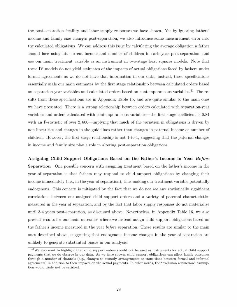
the post-separation fertility and labor supply responses we have shown. Yet by ignoring fathers’

income and family size changes post-separation, we also introduce some measurement error into

the calculated obligations. We can address this issue by calculating the average obligation a father

should face using his current income and number of children in each year post-separation, and

use our main treatment variable as an instrument in two-stage least squares models. Note that

these IV models do not yield estimates of the impacts of actual obligations faced by fathers under

formal agreements as we do not have that information in our data; instead, these specifications

essentially scale our main estimates by the first stage relationship between calculated orders based

on separation-year variables and calculated orders based on contemporaneous variables.41 The re-

sults from these specifications are in Appendix Table 15, and are quite similar to the main ones

we have presented. There is a strong relationship between orders calculated with separation-year

variables and orders calculated with contemporaneous variables—the first stage coefficient is 0.84

with an F-statistic of over 2, 600—implying that much of the variation in obligations is driven by

non-linearities and changes in the guidelines rather than changes in paternal income or number of

children. However, the first stage relationship is not 1-to-1, suggesting that the paternal changes

in income and family size play a role in altering post-separation obligations.

Assigning Child Support Obligations Based on the Father’s Income in Year Before

Separation One possible concern with assigning treatment based on the father’s income in the

year of separation is that fathers may respond to child support obligations by changing their

income immediately (i.e., in the year of separation), thus making our treatment variable potentially

endogenous. This concern is mitigated by the fact that we do not see any statistically significant

correlations between our assigned child support orders and a variety of parental characteristics

measured in the year of separation, and by the fact that labor supply responses do not materialize

until 3-4 years post-separation, as discussed above. Nevertheless, in Appendix Table 16, we also

present results for our main outcomes where we instead assign child support obligations based on

the father’s income measured in the year before separation. These results are similar to the main

ones described above, suggesting that endogenous income changes in the year of separation are

unlikely to generate substantial biases in our analysis.41We also want to highlight that child support orders should not be used as instruments for actual child support

payments that we do observe in our data. As we have shown, child support obligations can affect family outcomesthrough a number of channels (e.g., changes to custody arrangements or transitions between formal and informalagreements) in addition to their impacts on the actual payments. In other words, the “exclusion restriction” assump-tion would likely not be satisfied.

28

Page 30

Simpler “Double-Difference” Models Our main specification is a type of “triple-difference”

model that exploits variation across paternal incomes, number of children, and separation years.

We test the sensitivity of this specification by considering one- and two-child families separately

in analyses that only exploit variation in child support guidelines by year of separation and the

father’s income. These regressions still include the controls in vector Xit described above, as well as

fixed effects for the year of separation and 20, 000DKK bins in father’s income.42 Appendix Tables

17 and 18 present the results from these simpler “double-difference” type specifications. While we

lose some power and variation in these analyses, the effects are broadly consistent with the main

results reported above. Additionally, these results suggest that the effects of child support orders

on parental outcomes are similar across one- and two-child families.

7 Conclusion

As growing numbers of children in the United States and many Western European countries have

parents who are divorced or separated, understanding the causal effects of government interventions

into their families is important. Since unmarried and divorced mothers have historically retained

physical custody of their children and had full parental rights, most of these government inter-

ventions are centered around encouraging father involvement. These policies share the underlying

assumption that father involvement is essential to child well-being and seek to reduce public spend-

ing by shifting the burden of support of single-mother households from government programs to

the children’s fathers.

However, the implications of such policies for both child well-being and public budgets depend

crucially on their causal impacts on parental behavior. This type of research has thus far been

infeasible on a large scale in the United States primarily due to data constraints, and the Danish

context provides a unique opportunity to study these issues. We exploit Danish administrative data

together with non-linearities in child support guidelines that assign non-custodial parents different

obligations according to their incomes, numbers of children, and separation years to study the

causal effects of child support mandates on parental outcomes. We estimate that among parents

with a formal agreement, a 1, 000DKK increase in a father’s average annual child support obligation

is associated with about a 573DKK increase in the average annual child support payment.

We also show parental responses on other margins. In particular, higher orders reduce the42We also control for children aging out of child support by turning 18 by including fixed effects for the number of

children still under age 18 in each year post-separation (not including any new children born post-separation), as inour main regression equation.

29

Page 31

likelihood that fathers live with their children in at least one year post-separation, providing some

evidence of substitution between monetary and non-pecuniary paternal investments. Additionally,

we find that child support mandates increase post-separation fertility for both parents. While

both parents are more likely to have additional children while married to or cohabiting with new

partners, mothers are also more likely to have children outside these unions. The fertility effects

for mothers are consistent with a positive income-fertility relationship, while the fertility effects

for fathers are consistent with increased demand for new offspring as a result of reduced contact

with existing children. Finally, we find evidence that among higher-income fathers for whom child

support obligations represent taxes on earnings, higher orders are associated with reductions in

labor force participation and transitions into disability insurance and early retirement programs.

The findings in this paper point to important parental behavioral responses to redistributive

policies meant to address the needs of children growing up in so-called “broken homes”. By plac-

ing mandates on non-custodial parents to make financial transfers to their children, these policies

can disincentivize other forms of non-pecuniary involvement. Moreover, these obligations generate

shocks to parental income and time allocation, and can thus impact their subsequent family for-

mation decisions and the division of resources across children. As such, the net impacts on child

investment levels and overall child well-being are complicated and ambiguous. Our results cannot

directly speak to these implications, although future research might shed light on these issues by

exploring the effects of child support mandates on children’s cognitive and health outcomes.

The net effects on public spending are also potentially unclear. For example, the fact that some

fathers respond to obligations by exiting the labor force and taking up disability insurance or early

retirement benefits reveals a possible increase in public sector costs. In 2008, public expenditure

on disability pensions amounted to about 16.5 billion DKK ($3.1 billion) in Denmark.43 Given

that there were about 240, 000 recipients in that year, this translates to approximately 69, 000DKK

($13, 000) per recipient.44 Our estimated positive effect on the take-up of disability insurance alone

can thus be valued at approximately 21 million DKK ($4 million).45 Of course these increases

in public spending costs have to be weighed against any savings, such as those due to potential

reductions in maternal welfare benefit take-up, which we do not observe. Nevertheless, our findings

point to the possible unintended consequences of child support mandates on public budgets.43See OECD.Stat for more details: http://stats.oecd.org/Index.aspx?DataSetCode=SOCX_AGG.44In 2008, the Danish age 18-64 population was 3,418,273 according to Statistics Denmark, and approximately 7

percent of them were receiving disability income (Bingley et al., 2011). This amounts to 0.07 ∗ 3, 418, 273 = 239, 279recipients.

45This value is calculated as follows: We estimate a 0.00126 increase in the likelihood of disability insurancetake-up, which translates to 0.00126 ∗ 240, 000 = 302 additional recipients. This means that costs are increased by302 ∗ 69, 000DKK= 20, 838, 000DKK.

30

Page 32

References

Aizer, A. and McLanahan, S. (2006). The impact of child support enforcement on fertility,parental investments, and child well-being. Journal of Human Resources, 41 (1), 28–45.

Autor, D. and Duggan, M. (2003). The rise in the disability rolls and the decline in unemploy-ment. The Quarterly Journal of Economics, 118 (1), 157–206.

Bingley, P., Gupta, N. D. and Pedersen, P. J. (2011). Disability Programs, Health and Re-tirement in Denmark since 1960. Working Paper 17138, National Bureau of Economic Research.

Bjarnason, T. and Arnarsson, A. M. (2011). Joint physical custody and communication withparents: a cross-national study of children in 36 western countries. Journal of Comparative FamilyStudies, pp. 871–890.

Black, D., Daniel, K. and Sanders, S. (2002). The impact of economic conditions on participa-tion in disability programs: Evidence from the coal boom and bust. American Economic Review,pp. 27–50.

Bloom, D. E., Conrad, C. and Miller, C. (1998). Child support and fathers’ remarriage andfertility. In I. Garfinkel, S. McLanahan, D. Meyer and J. Seltzer (eds.), Fathers Under Fire: TheRevolution in Child Support Enforcement, New York: Russell Sage Foundation, pp. 128–150.

Bratsberg, B., Fevang, E. and Røed, K. (2010). Disability in the welfare state: An unemploy-ment problem in disguise? Tech. Rep. 4897, Institute for the Study of Labor (IZA).

Brewer, M., Ratcliffe, A. and Smith, S. (2012). Does welfare reform affect fertility? evidencefrom the uk. Journal of Population Economics, 25 (1), 245–266.

Brown, M. and Flinn, C. J. (2011). Family law effects on divorce, fertility and child investment,New York University, unpublished manuscript.

Cancian, M., Heinrich, C. and Chung, Y. (2013). Discouraging disadvantaged fathers’ em-ployment: An unintended consequence of policies designed to support families. Journal of PolicyAnalysis and Management, 32 (4), 758–784.

—, Meyer, D. and Roff, J. (2007). Testing New Ways to Increase the Economic Well-Being ofSingle-Parent Families: The Effects of Child Support Policies on Welfare Participants. DiscussionPaper 1330-07, Institute for Research on Poverty.

— and Meyer, D. R. (2014). Testing the economic independence hypothesis: The effect of an ex-ogenous increase in child support on subsequent marriage and cohabitation. Demography, 51 (3),857–880.

—, — and Han, E. (2011). Child support: responsible fatherhood and the quid pro quo. TheANNALS of the American Academy of Political and Social Science, 635 (1), 140–162.

Case, A. (1998). The effects of stronger child support enforcement on nonmarital fertility. InI. Garfinkel, S. McLanahan, D. Meyer and J. Seltzer (eds.), Fathers under fire: The revolutionin child support enforcement, New York: Russell Sage Foundation, pp. 191–215.

Dahl, G. B. and Lochner, L. (2012). The impact of family income on child achievement: Evi-dence from the earned income tax credit. American Economic Review, 102 (5), 1927–1956.

Del Boca, D. (2003). Mothers, fathers, and children after divorce: The role of institutions. Journalof Population Economics, 16, 399–422.

— and Flinn, C. J. (1995). Rationalizing child-support decisions. The American Economic Review,pp. 1241–1262.

— and Ribero, R. (2003). Visitations and transfers after divorce. Review of the Economics of theHousehold, 1, 187–204.

31

Page 33

Flinn, C. J. (2000). Modes of interaction between divorced parents. International Economic Re-view, 41 (3), 545–578.

Freeman, R. B. and Waldfogel, J. (1998). Does child support enforcement policy affect malelabor supply. In I. Garfinkel, S. McLanahan, D. Meyer and J. Seltzer (eds.), Fathers Under Fire:The Revolution in Child Support Enforcement, New York: Russell Sage Foundation, pp. 94–127.

— and — (2001). Dunning delinquent dads: The effects of child support enforcement policy onchild support receipt by never married women. Journal of Human Resources, 36 (2), 207–225.

Garfinkel, I., Mclanahan, S., Meyer, D. and Seltzer, J. (1998). Fathers under fire: Therevolution in child support enforcement. Russell Sage Foundation Publications.

—, Melli, M. S. and Robertson, J. G. (1994). Child support orders: A perspective on reform.The Future of Children, pp. 84–100.

Gruber, J. (2000). Disability insurance benefits and labor supply. The Journal of Political Econ-omy, 108 (6), 1162–1183.

— and Saez, E. (2002). The elasticity of taxable income: evidence and implications. Journal ofpublic Economics, 84 (1), 1–32.

— and Wise, D. A. (2004). Social Security Programs and Retirement around the World: Micro-Estimation. University of Chicago press.

— and — (2009). Social security programs and retirement around the world: Fiscal implications ofreform. University of Chicago press.

Gunter, S. P. (2013). Effects of child support pass-through and disregard policies on in-kind childsupport. Review of Economics of the Household, 11 (2), 193–209.

Halla, M. (2013). The effect of joint custody on family outcomes. Journal of the European Eco-nomic Association, 11 (2), 278–315.

Holzer, H. J., Offner, P. and Sorensen, E. (2005). Declining employment among young blackless-educated men: The role of incarceration and child support. Journal of Policy Analysis andManagement, 24 (2), 329–350.

Hoynes, H. W. (1997). Work, welfare, and family structure: What have we learned? In A. Auer-bach (ed.), Fiscal Policy: Lessons from Economic Research, MIT Press, pp. 101–146.

Huang, C.-C. (2002). The impact of child support enforcement on nonmarital and marital births:Does it differ by racial and age groups? Social Service Review, 76 (2), 275–301.

Kampmann, J. and Nielsen, H. W. (2004). Socialized childhood: Children’s childhoods in Den-mark. In A.-M. Jensen, A. Ben-Arieh, C. Conti, M. N. Ghiolla Phadraig and H. W. Nielsen(eds.), Children’s Welfare in Ageing Europe, vol. 2, pp. 649–702.

Laroque, G. and Salanié, B. (2008). Does fertility respond to financial incentives? DiscussionPaper 3575, Institute for the Study of Labor (IZA).

Larsen, M. and Pedersen, P. J. (2012). Paid Work after Retirement: Recent Trends in Denmark.Discussion Paper 6537.

Lerman, R. I. and Sorenson, E. (2003). Child support: Interactions between private and publictransfers. In Means-tested transfer programs in the United States, University of Chicago Press,pp. 587–628.

Milligan, K. (2005). Subsidizing the stork: New evidence on tax incentives and fertility. Reviewof Economics and Statistics, 87 (3), 539–555.

32

Page 34

— and Stabile, M. (2011). Do child tax benefits affect the well-being of children? evidencefrom canadian child benefit expansions. American Economic Journal: Economic Policy, 3 (3),175–205.

Moffitt, R. (2002). Welfare programs and labor supply. In A. Auerbach and M. Feldstein (eds.),Handbook of Public Economics, vol. 4, Elsevier, pp. 2393–2430.

Moffitt, R. A. (1998). The effect of welfare on marriage and fertility. In R. A. Moffitt (ed.),Welfare, the Family, and Reproductive Behavior:: Research Perspectives, National AcademiesPress, p. 50.

Neal, D. (2004). The relationship between marriage market prospects and never-married mother-hood. Journal of Human Resources, 39 (4), 938–957.

Nepomnyaschy, L. (2007). Child support and father-child contact: Testing reciprocal pathways.Demography, 44 (1), 93–112.

— and Garfinkel, I. (2010). Child support enforcement and fathers’ contributions to their non-marital children. The Social service review, 84 (3), 341.

Piketty, T. and Saez, E. (2013). Optimal labor income taxation. In A. J. Auerbach, R. Chetty,M. Feldstein and E. Saez (eds.), Handbook of Public Economics, vol. 5, pp. 391–474.

Plotnick, R. D., Garfinkel, I., McLanahan, S. S. and Ku, I. (2004). Better child supportenforcement can it reduce teenage premarital childbearing? Journal of Family Issues, 25 (5),634–657.

Roff, J. and Lugo-Gil, J. (2012). A model of child support and the underground economy.Labour Economics, 19 (5), 668–681.

Saez, E., Slemrod, J. and Giertz, S. H. (2012). The elasticity of taxable income with respectto marginal tax rates: A critical review. Journal of Economic Literature, 50 (1), 3–50.

Schoeni, R. and Blank, R. (2000). What has welfare reform accomplished? Impacts on welfareparticipation, employment, income, poverty, and family structure. Working Paper 7627, NationalBureau of Economic Research.

Skinner, C., Bradshaw, J. and Davidson, J. (2007). Child Support Policy: An InternationalPerspective. Research report, Department for Work and Pensions.

Sorensen, E. and Halpern, A. (1999). Child support enforcement: How well is it doing? Dis-cussion Paper 99-11, The Urban Institute.

— and Olivier, H. (2002). Child support reforms in PRWORA: Initial impacts. Discussion Paper02-02, The Urban Institute.

Stevenson, B. and Wolfers, J. (2006). Bargaining in the shadow of the law: Divorce laws andfamily distress. The Quarterly Journal of Economics, 121 (1), 267–288.

Tartari, M. (2014). Divorce and the cognitive achievement of children, University of Chicago,unpublished manuscript.

Weinberg, D. H. (2006). Income data quality issues in the CPS. Monthly Labor Review, 129, 38.

Weiss, Y. and Willis, R. (1985). Children as collective goods and divorce settlements. Journalof Labor Economics, 3 (3), 268–292.

Willis, R. J. (1999). A theory of out-of-wedlock childbearing. Journal of Political Economy,107 (S6), S33–S64.

Wolfers, J. (2006). Did unilateral divorce laws raise divorce rates? a reconciliation and newresults. The American Economic Review, 96 (5), 1802–1820.

33

Page 35

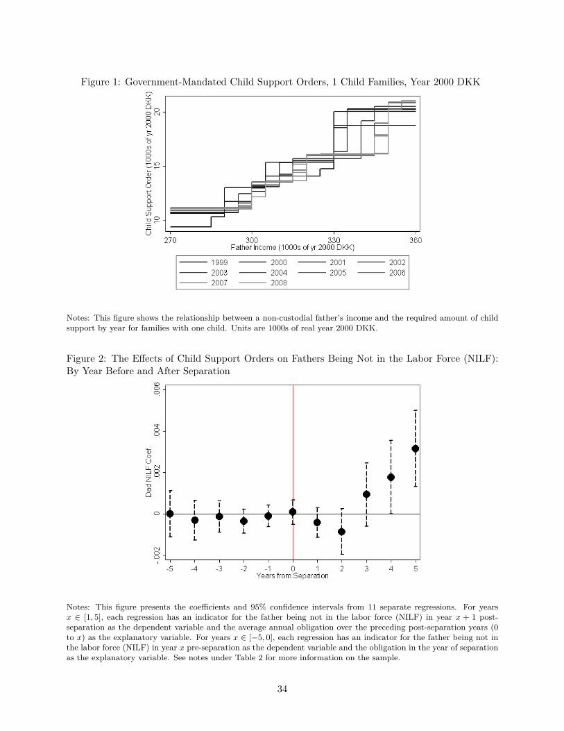
Figure 1: Government-Mandated Child Support Orders, 1 Child Families, Year 2000 DKK

Notes: This figure shows the relationship between a non-custodial father’s income and the required amount of childsupport by year for families with one child. Units are 1000s of real year 2000 DKK.

Figure 2: The Effects of Child Support Orders on Fathers Being Not in the Labor Force (NILF):By Year Before and After Separation

Notes: This figure presents the coefficients and 95% confidence intervals from 11 separate regressions. For yearsx ∈ [1, 5], each regression has an indicator for the father being not in the labor force (NILF) in year x + 1 post-separation as the dependent variable and the average annual obligation over the preceding post-separation years (0to x) as the explanatory variable. For years x ∈ [−5, 0], each regression has an indicator for the father being not inthe labor force (NILF) in year x pre-separation as the dependent variable and the obligation in the year of separationas the explanatory variable. See notes under Table 2 for more information on the sample.

34

Page 36

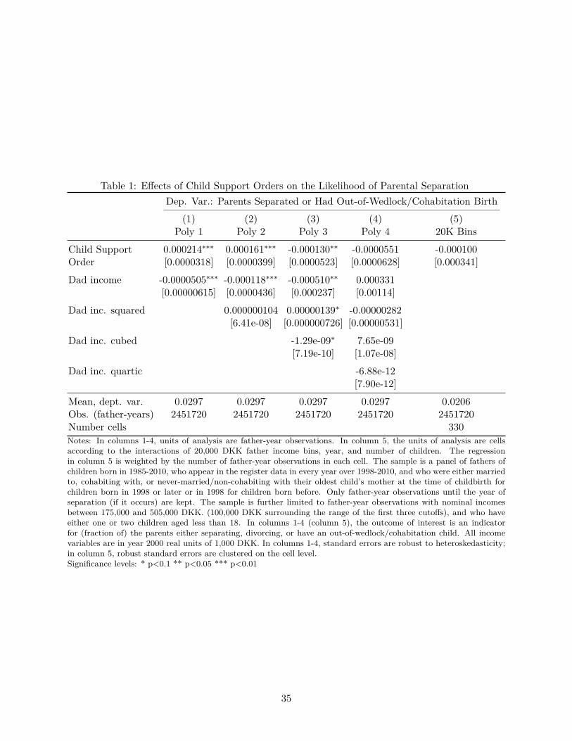
Table 1: Effects of Child Support Orders on the Likelihood of Parental SeparationDep. Var.: Parents Separated or Had Out-of-Wedlock/Cohabitation Birth

(1) (2) (3) (4) (5)Poly 1 Poly 2 Poly 3 Poly 4 20K Bins

Child Support 0.000214∗∗∗ 0.000161∗∗∗ -0.000130∗∗ -0.0000551 -0.000100Order [0.0000318] [0.0000399] [0.0000523] [0.0000628] [0.000341]

Dad income -0.0000505∗∗∗ -0.000118∗∗∗ -0.000510∗∗ 0.000331[0.00000615] [0.0000436] [0.000237] [0.00114]

Dad inc. squared 0.000000104 0.00000139∗ -0.00000282[6.41e-08] [0.000000726] [0.00000531]

Dad inc. cubed -1.29e-09∗ 7.65e-09[7.19e-10] [1.07e-08]

Dad inc. quartic -6.88e-12[7.90e-12]

Mean, dept. var. 0.0297 0.0297 0.0297 0.0297 0.0206Obs. (father-years) 2451720 2451720 2451720 2451720 2451720Number cells 330Notes: In columns 1-4, units of analysis are father-year observations. In column 5, the units of analysis are cellsaccording to the interactions of 20,000 DKK father income bins, year, and number of children. The regressionin column 5 is weighted by the number of father-year observations in each cell. The sample is a panel of fathers ofchildren born in 1985-2010, who appear in the register data in every year over 1998-2010, and who were either marriedto, cohabiting with, or never-married/non-cohabiting with their oldest child’s mother at the time of childbirth forchildren born in 1998 or later or in 1998 for children born before. Only father-year observations until the year ofseparation (if it occurs) are kept. The sample is further limited to father-year observations with nominal incomesbetween 175,000 and 505,000 DKK. (100,000 DKK surrounding the range of the first three cutoffs), and who haveeither one or two children aged less than 18. In columns 1-4 (column 5), the outcome of interest is an indicatorfor (fraction of) the parents either separating, divorcing, or have an out-of-wedlock/cohabitation child. All incomevariables are in year 2000 real units of 1,000 DKK. In columns 1-4, standard errors are robust to heteroskedasticity;in column 5, robust standard errors are clustered on the cell level.Significance levels: * p<0.1 ** p<0.05 *** p<0.01

35

Page 37

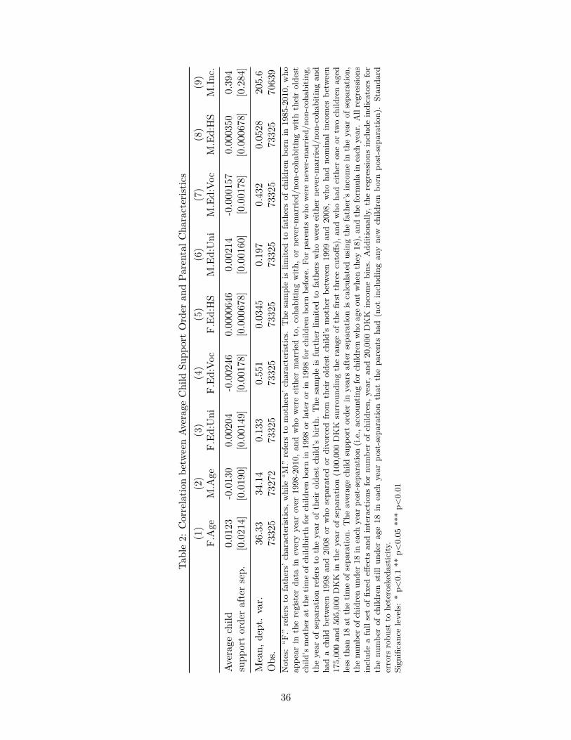
Table2:

Correlatio

nbe

tweenAv

erag

eChild

Supp

ortOrder

andPa

rental

Cha

racterist

ics

(1)

(2)

(3)

(4)

(5)

(6)

(7)

(8)

(9)

F.Age

M.A

geF.Ed

:Uni

F.Ed

:Voc

F.Ed

:HS

M.Ed:Uni

M.Ed:Vo

cM.Ed:HS

M.In

c.

Averag

echild

0.01

23-0.013

00.00

204

-0.002

460.00

0064

60.00

214

-0.000

157

0.00

0350

0.39

4supp

ortorde

raftersep.

[0.021

4][0.019

0][0.001

49]

[0.001

78]

[0.000

678]

[0.001

60]

[0.001

78]

[0.000

678]

[0.284

]

Mean,

dept.var.

36.33

34.14

0.13

30.55

10.03

450.19

70.43

20.05

2820

5.6

Obs.

7332

573

272

7332

573

325

7332

573

325

7332

573

325

7063

9Notes:“F

.”refers

tofathers’

characteris

tics,

while

“M.”refers

tomothe

rs’c

haracteristic

s.The

sampleis

limite

dto

fathersof

child

renbo

rnin

1985-2010,

who

appe

arin

theregister

data

ineveryyear

over

1998-2010,

andwho

wereeither

marrie

dto,coha

bitin

gwith

,or

never-marrie

d/no

n-coha

bitin

gwith

theirolde

stchild

’smothe

rat

thetim

eof

child

birthforchild

renbo

rnin

1998

orlateror

in1998

forchild

renbo

rnbe

fore.Fo

rpa

rentswho

werenever-marrie

d/no

n-coha

bitin

g,theyear

ofsepa

ratio

nrefers

totheyear

oftheirolde

stchild

’sbirth.

The

sampleis

furthe

rlim

itedto

fatherswho

wereeither

never-marrie

d/no

n-coha

bitin

gan

dha

dachild

betw

een1998

and2008

orwho

sepa

ratedor

divo

rced

from

theirolde

stchild

’smothe

rbe

tween1999

and2008,who

hadno

minal

incomes

betw

een

175,000an

d505,000DKK

intheyear

ofsepa

ratio

n(100,000

DKK

surrou

ndingtherang

eof

thefirst

threecutoffs),an

dwho

hadeither

oneor

twochild

renaged

less

than

18at

thetim

eof

sepa

ratio

n.The

averagechild

supp

ortorde

rin

yearsaftersepa

ratio

nis

calculated

usingthefather’s

incomein

theyear

ofsepa

ratio

n,thenu

mbe

rof

chidrenun

der18

ineach

year

post-sep

aration(i.e.,a

ccou

ntingforchild

renwho

ageou

twhe

nthey

18),an

dtheform

ulain

each

year.Allregression

sinclud

eafullsetof

fixed

effects

andinteractions

fornu

mbe

rof

child

ren,

year,a

nd20,000

DKK

incomebins.Add

ition

ally,t

heregression

sinclud

eindicators

for

thenu

mbe

rof

child

renstill

unde

rage18

ineach

year

post-sep

arationthat

thepa

rentsha

d(not

includ

ingan

yne

wchild

renbo

rnpo

st-sep

aration).Stan

dard

errors

robu

stto

heterosked

astic

ity.

Sign

ificancelevels:*p<

0.1**

p<0.05

***p<

0.01

36

Page 38

Table 3: Effects of Average Child Support Orders on Fathers’ Child Support Payments and Father-Child Co-Residence

(1) (2) (3)Average CS Zero CS Ever Ever live w/child

Average child 0.427∗∗∗ -0.0112∗∗∗ -0.00494∗∗∗support order after sep. [0.0317] [0.00123] [0.00171]

Mean, dept. var. 9.252 0.737 0.278Obs. 70639 70639 70639Notes: The outcomes are defined as follows: 1) “Average CS” refers to the average annual child support paid by thefather in the years post-separation; 2) “Zero CS Ever” refers to an indicator for zero child support paid by the fatherin at least one year post-separation; 3) “Ever live w/child” refers to an indicator for the father living with the child atleast one year post-separation. All income variables are in year 2000 real units of 1,000 DKK. See notes under Table2 for more information on the sample. All regressions include fixed effects for 20,000 DKK bins in father’s income,number of children, year of separation, and their double interactions. All regressions include controls (measured inthe year of separation) for the father’s age and age squared, dummies for the father’s education (less than high school,high school, vocational/short-term higher ed, college/university, and missing), an indicator for the father being fromWestern Europe, mother’s age and age squared, dummies for the mother’s education (less than high school, highschool, vocational/short-term higher ed, college/university, and missing), an indicator for the mother being fromWestern Europe, mother’s total income in year 2000 DKK, oldest child’s age and age squared, youngest child’s ageand age squared, and indicators for original parental relationship status (married, cohabiting, never-married/non-cohabiting). Additionally, the regressions include indicators for the number of children still under age 18 in each yearpost-separation that the parents had (not including any new children born post-separation). Standard errors robustto heteroskedasticity.Significance levels: * p<0.1 ** p<0.05 *** p<0.01

37

Page 39

Table 4: Effects of Average Child Support Orders on Mothers’ Post-Separation Fertility OutcomesMother Has More Kids After Sep.

(1) (2) (3) (4)Overall Mar. Coh. Not Mar./Coh.

Average child 0.00505∗∗∗ 0.00318∗∗∗ 0.00123∗∗ 0.000699∗∗support order after sep. [0.000844] [0.000593] [0.000625] [0.000314]

Mean, dept. var. 0.185 0.0657 0.0921 0.0287Obs. 68941 68941 68941 68941Notes: The outcomes are defined as follows: 1) “Overall” refers to an indicator for the mother having any childrenpost-separation (regardless of relationship status); 2) “Mar.” refers to an indicator for the mother having morechildren post-separation while married to a new partner; 3) “Coh.” refers to an indicator for the mother having morechildren post-separation while cohabiting with a new partner; 4) “Not Mar./Coh.” refers to an indicator for themother having more children post-separation while neither married or cohabiting. All income variables are in year2000 real units of 1,000 DKK. See notes under Tables 2 and 3 for more information on the sample, specifications,and controls. Standard errors robust to heteroskedasticity.Significance levels: * p<0.1 ** p<0.05 *** p<0.01

Table 5: Effects of Average Child Support Orders on Fathers’ Post-Separation Fertility OutcomesFather Has More Kids After Sep.

(1) (2) (3) (4) (5)Overall Mar. Coh. Not Mar./Coh. Not living w/ older child

Average child 0.00582∗∗∗ 0.00273∗∗∗ 0.00279∗∗∗ 0.000234 0.00640∗∗∗support order after sep. [0.00102] [0.000753] [0.000709] [0.000384] [0.000914]

Mean, dept. var. 0.186 0.0804 0.0830 0.0238 0.148Obs. 70639 70639 70639 70639 70639Notes: The outcomes are defined as follows: 1) “Overall” refers to an indicator for the father having any childrenpost-separation (regardless of relationship status); 2) “Mar.” refers to an indicator for the father having more childrenpost-separation while married to a new partner; 3) “Coh.” refers to an indicator for the father having more childrenpost-separation while cohabiting with a new partner; 4) “Not Mar./Coh.” refers to an indicator for the father havingmore children post-separation while neither married or cohabiting; 5) “Not living w/ older child” refers to an indicatorfor the father having more children post-separation while not living with his oldest child. All income variables are inyear 2000 real units of 1,000 DKK. See notes under Tables 2 and 3 for more information on the sample, specifications,and controls. Standard errors robust to heteroskedasticity.Significance levels: * p<0.1 ** p<0.05 *** p<0.01

38

Page 40

Table6:

Effects

ofAv

erag

eChild

Supp

ortOrderson

Fathers’

Post-Sep

arationLa

borMarketOutcomes

(1)

(2)

(3)

(4)

(5)

(6)

(7)

(8)

Any

Wag

eLo

gWag

eEm

p.Se

lf-Em

p.NILF

Dis.

Welf.

Ret.

Averag

echild

-0.001

39∗

-0.001

06-0.000

639

-0.000

335

0.00

176∗∗∗

0.00

103∗∗∗

-0.000

116

0.00

102∗∗∗

supp

ortorde

raftersep.

[0.000

827]

[0.003

90]

[0.000

996]

[0.000

842]

[0.000

458]

[0.000

298]

[0.000

263]

[0.000

256]

Mean,

dept.var.

0.91

512

.26

0.83

20.06

110.04

180.01

130.02

490.00

364

Obs.

7062

669

184

7063

970

639

7063

970

639

7063

970

639

Notes:The

outcom

esarede

fined

asfollo

ws:

1)“A

nyWage”

refers

totheprop

ortio

nof

yearsthefather

hasan

ywageincomepo

st-sep

aration,

2)“L

ogWage”

refers

tothelogof

thefather’s

averagean

nual

wageincomein

theyearspo

st-sep

aration,

3)“E

mp.”

refers

totheprop

ortio

nof

yearsthefather

isem

ployed

intheprivateor

public

sector

(not

self-em

ployed

)po

st-sep

aration,

4)“S

elf-E

mp.”

refers

totheprop

ortio

nof

yearsthefather

isself-em

ployed

post-sep

aration,

5)“N

ILF”

refers

totheprop

ortio

nof

yearsthefather

isno

tin

thelabo

rforcepo

st-separation,

6)“D

is.”

refers

totheprop

ortio

nof

yearsthefather

isno

tin

the

labo

rforcedu

eto

disabilityleavepo

st-sep

aration,

7)“W

elf.”

refers

totheprop

ortio

nof

yearsthefather

isno

tin

thelabo

rforcean

dreceivingwelfare

bene

fits,

and8)

“Ret.”

refers

totheprop

ortio

nof

yearsthefather

isno

tin

thelabo

rforcedu

eto

retir

ement(in

clud

ingearly

retir

ement)

post-sep

aration.

Allincome

varia

bles

arein

year

2000

real

units

of1,000DKK.S

eeno

tesun

derTa

bles

2an

d3formoreinform

ationon

thesample,

specificatio

ns,a

ndcontrols.Stan

dard

errors

robu

stto

heterosked

astic

ity.

Sign

ificancelevels:*p<

0.1**

p<0.05

***p<

0.01

39

Page 41

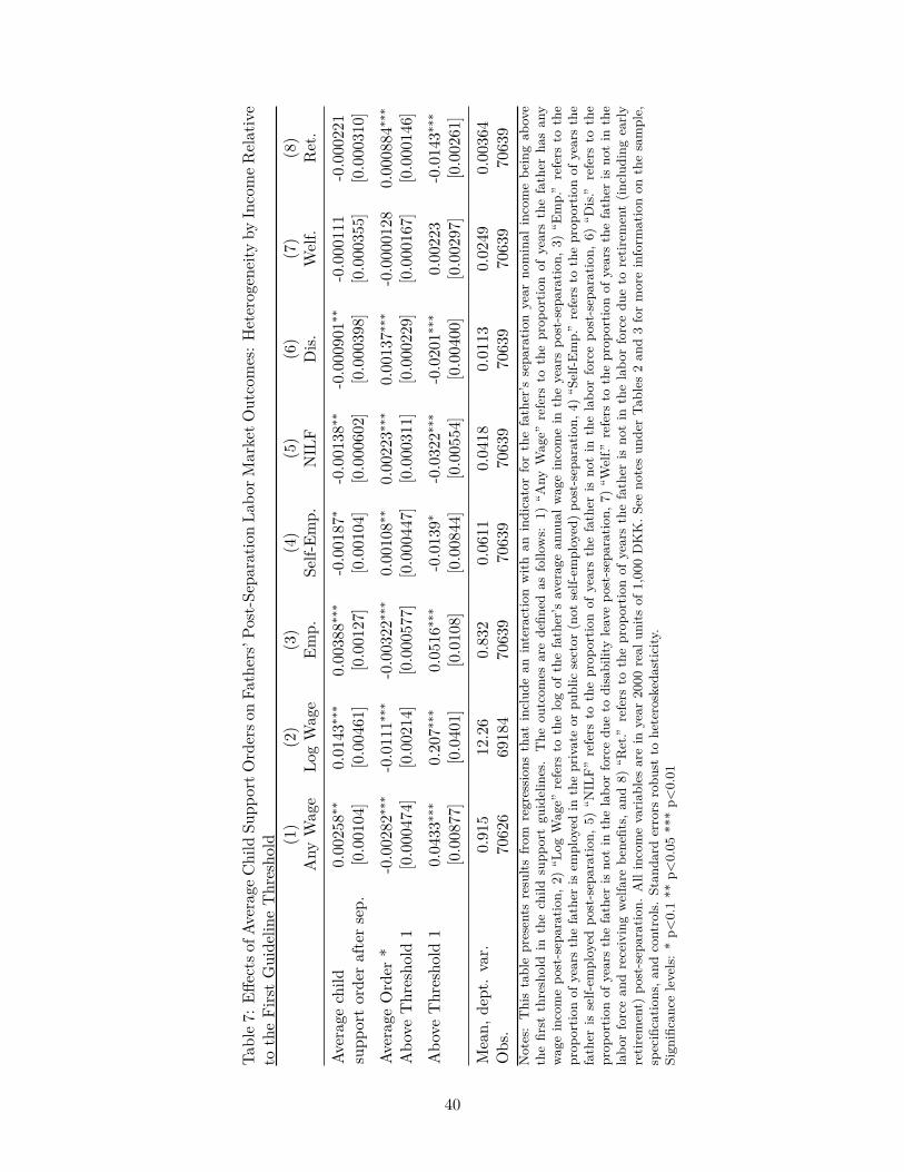
Table7:

Effects

ofAv

erag

eChild

Supp

ortO

rderso

nFa

thers’Po

st-Sep

arationLa

borM

arketO

utcomes:H

eterog

eneity

byIncomeRelative

totheFirstGuide

lineThresho

ld (1)

(2)

(3)

(4)

(5)

(6)

(7)

(8)

Any

Wag

eLo

gWag

eEm

p.Se

lf-Em

p.NILF

Dis.

Welf.

Ret.

Averag

echild

0.00

258∗∗

0.01

43∗∗∗

0.00

388∗∗∗

-0.001

87∗

-0.001

38∗∗

-0.000

901∗∗

-0.000

111

-0.000

221

supp

ortorde

raftersep.

[0.001

04]

[0.004

61]

[0.001

27]

[0.001

04]

[0.000

602]

[0.000

398]

[0.000

355]

[0.000

310]

Averag

eOrder

*-0.002

82∗∗∗

-0.011

1∗∗∗

-0.003

22∗∗∗

0.00

108∗∗

0.00

223∗∗∗

0.00

137∗∗∗

-0.000

0128

0.00

0884∗∗∗

Abo

veThresho

ld1

[0.000

474]

[0.002

14]

[0.000

577]

[0.000

447]

[0.000

311]

[0.000

229]

[0.000

167]

[0.000

146]

Abo

veThresho

ld1

0.04

33∗∗∗

0.20

7∗∗∗

0.05

16∗∗∗

-0.013

9∗-0.032

2∗∗∗

-0.020

1∗∗∗

0.00

223

-0.014

3∗∗∗

[0.008

77]

[0.040

1][0.010

8][0.008

44]

[0.005

54]

[0.004

00]

[0.002

97]

[0.002

61]

Mean,

dept.var.

0.91

512

.26

0.83

20.06

110.04

180.01

130.02

490.00

364

Obs.

7062

669

184

7063

970

639

7063

970

639

7063

970

639

Notes:Thistablepresents

results

from

regression

sthat

includ

ean

interactionwith

anindicatorforthefather’s

sepa

ratio

nyear

nominal

incomebe

ingab

ove

thefirst

thresholdin

thechild

supp

ortgu

idelines.The

outcom

esarede

fined

asfollo

ws:

1)“A

nyWage”

refers

totheprop

ortio

nof

yearsthefather

hasan

ywageincomepo

st-sep

aration,

2)“L

ogWage”

refers

tothelogof

thefather’s

averagean

nual

wageincomein

theyearspo

st-sep

aration,

3)“E

mp.”

refers

tothe

prop

ortio

nof

yearsthefather

isem

ployed

intheprivateor

public

sector

(not

self-em

ployed

)po

st-sep

aration,

4)“S

elf-E

mp.”refers

totheprop

ortio

nof

yearsthe

father

isself-em

ployed

post-sep

aration,

5)“N

ILF”

refers

totheprop

ortio

nof

yearsthefather

isno

tin

thelabo

rforcepo

st-sep

aration,

6)“D

is.”

refers

tothe

prop

ortio

nof

yearsthefather

isno

tin

thelabo

rforcedu

eto

disabilityleavepo

st-sep

aration,

7)“W

elf.”

refers

totheprop

ortio

nof

yearsthefather

isno

tin

the

labo

rforcean

dreceivingwelfare

bene

fits,

and8)

“Ret.”

refers

totheprop

ortio

nof

yearsthefather

isno

tin

thelabo

rforcedu

eto

retir

ement(in

clud

ingearly

retir

ement)

post-sep

aration.

Allincomevaria

bles

arein

year

2000

real

units

of1,000DKK.S

eeno

tesun

derTa

bles

2an

d3formoreinform

ationon

thesample,

specificatio

ns,a

ndcontrols.Stan

dard

errors

robu

stto

heterosked

astic

ity.

Sign

ificancelevels:*p<

0.1**

p<0.05

***p<

0.01

40

Page 42

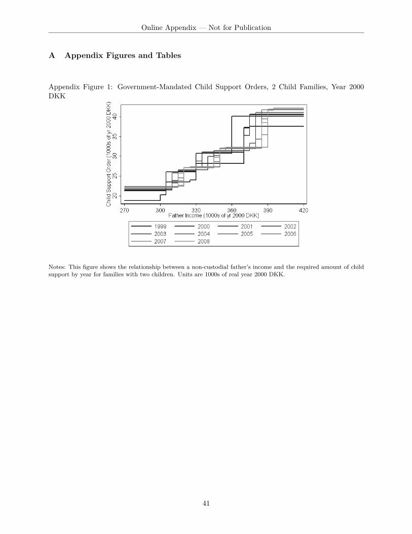
Online Appendix — Not for Publication

A Appendix Figures and Tables

Appendix Figure 1: Government-Mandated Child Support Orders, 2 Child Families, Year 2000DKK

Notes: This figure shows the relationship between a non-custodial father’s income and the required amount of childsupport by year for families with two children. Units are 1000s of real year 2000 DKK.

41

Page 43

Appendix Figure 2: Government-Mandated Child Support Orders, 1 Child Families, Nominal DKK

Notes: This figure shows the relationship between a non-custodial father’s income and the required amount of childsupport by year for families with one child. Units are 1000s of nominal DKK.

Appendix Figure 3: Government-Mandated Child Support Orders, 2 Child Families, Nominal DKK

Notes: This figure shows the relationship between a non-custodial father’s income and the required amount of childsupport by year for families with two children. Units are 1000s of nominal DKK.

42

Page 44

Appendix Figure 4: The Effects of Child Support Orders on Paternal Physical Custody: By YearAfter Separation

Notes: This figure presents the coefficients and 95% confidence intervals from five separate regressions. In particular,for years x ∈ [1, 5]—the first five years of separation displayed on the x-axis—each regression has an indicator forthe father living with his oldest child in year x + 1 post-separation as the dependent variable and the average annualobligation over the preceding post-separation years (0 to x) as the explanatory variable. See notes under Table 2for more information on the sample. All regressions include fixed effects for 20,000 DKK bins in father’s income,number of children, year of separation, and their double interactions. All regressions include controls (measured inthe year of separation) for the father’s age and age squared, dummies for the father’s education (less than high school,high school, vocational/short-term higher ed, college/university, and missing), an indicator for the father being fromWestern Europe, mother’s age and age squared, dummies for the mother’s education (less than high school, highschool, vocational/short-term higher ed, college/university, and missing), an indicator for the mother being fromWestern Europe, mother’s total income in year 2000 DKK, oldest child’s age and age squared, youngest child’s ageand age squared, and indicators for original parental relationship status (married, cohabiting, never-married/non-cohabiting). Additionally, the regressions include indicators for the number of children still under age 18 in each yearpost-separation that the parents had (not including any new children born post-separation). Standard errors robustto heteroskedasticity.

43

Page 45

Appendix Figure 5: The Effects of Child Support Orders on Mothers’ Subsequent Fertility: ByYear After Separation

Notes: This figure presents the coefficients and 95% confidence intervals from five separate regressions. In particular,for years x ∈ [1, 5]—the first five years of separation displayed on the x-axis—each regression has an indicator forthe mother having more children in year x + 1 post-separation as the dependent variable and the average annualobligation over the preceding post-separation years (0 to x) as the explanatory variable. See notes under Table 2 formore information on the sample, and notes under Appendix Figure 4 for more information on the estimation andcontrols.

44

Page 46

Appendix Figure 6: The Effects of Child Support Orders on Fathers’ Subsequent Fertility: By YearAfter Separation

Notes: This figure presents the coefficients and 95% confidence intervals from five separate regressions. In particular,for years x ∈ [1, 5]—the first five years of separation displayed on the x-axis—each regression has an indicator for thefather having more children in year x+1 post-separation as the dependent variable and the average annual obligationover the preceding post-separation years (0 to x) as the explanatory variable. See notes under Table 2 for moreinformation on the sample, and notes under Appendix Figure 4 for more information on the estimation and controls.

45

Page 47

Appendix Table 1: Child Support Obligation Schemes: 1999, 2005, 20081999: Normal Amount = 9,132 DKK; Extra Amount = 0 DKKObligation Income Range (1 Child) Income Range (2 Children)

Normal <=275,000 <=290,000Normal + 25% × Normal 275,001-290,000 290,001-315,000Normal + 50% × Normal 290,001-315,000 315,001-355,000Normal + 100% × Normal >315,000 >355,000

2005: Normal Amount = 10,824 DKK; Extra Amount = 1,392 DKKObligation Income Range (1 Child) Income Range (2 Children)

Normal + Extra <=325,000 <=345,000Normal + Extra + 25% × Normal 325,001-345,000 345,001-380,000Normal + Extra + 50% × Normal 345,001-380,000 380,001-420,000Normal + Extra + 100% × Normal 380,001-500,000 420,001-600,000Normal + Extra + 200% × Normal 500,001-900,000 600,001-1,100,000Normal + Extra + 300% × Normal >900,000 >1,100,000

2008: Normal Amount = 11,628 DKK; Extra Amount = 1,500 DKKObligation Income Range (1 Child) Income Range (2 Children)

Normal + Extra <=350,000 <=370,000Normal + Extra + 25% × Normal 350,001-370,000 370,001-405,000Normal + Extra + 50% × Normal 370,001-405,000 405,001-450,000Normal + Extra + 100% × Normal 405,001-600,000 450,001-700,000Normal + Extra + 200% × Normal 600,001-1,000,000 700,001-1,200,000Normal + Extra + 300% × Normal >1,000,000 >1,200,000

Notes: Information on the child support schemes comes from from Statsforvaltningen. For more information, pleasesee http://www.statsforvaltningen.dk/site.aspx?p=6404.

46

Page 48

Appendix Table 2: Summary Statistics(1) (2) (3) (4)

All Sep. Prev. Mar. Prev. Coh. Never Mar/Coh

Average child 9.211 10.19 9.025 5.735support paid after sep. (8.509) (9.529) (7.711) (5.136)

Average child 16.83 17.54 17.22 12.42support order after sep. (7.688) (8.467) (7.255) (2.790)

Average tax-ded. 15.18 15.86 15.48 11.15child support order after sep. (7.126) (7.847) (6.715) (2.788)

1st child’s age at 6.922 9.647 5.682 0sep. (5.586) (5.421) (4.335) (0)

Dad age at sep. 36.33 39.69 34.34 29.50(7.581) (7.060) (6.532) (5.972)

Dad inc. at sep. 286.3 298.6 279.7 258.6(71.92) (72.88) (68.73) (68.45)

Dad ed: uni/college 0.133 0.161 0.111 0.0939(0.339) (0.368) (0.314) (0.292)

Dad ed: short 0.551 0.565 0.554 0.476high-ed/vocational (0.497) (0.496) (0.497) (0.499)

Dad ed: high school 0.0345 0.0355 0.0303 0.0463(0.183) (0.185) (0.171) (0.210)

Dad from W. Europe 0.971 0.960 0.987 0.955(0.169) (0.197) (0.114) (0.206)

Mom age at sep. 34.14 37.17 32.40 27.78(7.111) (6.335) (6.497) (5.934)

Mom inc. at sep. 205.6 224.7 196.2 161.2(73.19) (73.07) (68.48) (63.97)

Mom ed: uni/college 0.197 0.231 0.176 0.133(0.398) (0.422) (0.381) (0.339)

Mom ed: short 0.432 0.481 0.416 0.287high-ed/vocational (0.495) (0.500) (0.493) (0.452)

Mom ed: high school 0.0528 0.0454 0.0547 0.0769(0.224) (0.208) (0.227) (0.266)

Mom from W. Europe 0.967 0.950 0.989 0.959(0.178) (0.218) (0.102) (0.197)

Obs. 73,325 34,663 30,481 8,181Notes: All income variables are in year 2000 real units of 1,000 DKK. The sample is limited to fathers of children bornin 1985-2010, who appear in the register data in every year over 1998-2010, and who were either married to, cohabitingwith, or never-married/non-cohabiting with their oldest child’s mother at the time of childbirth for children born in1998 or later or in 1998 for children born before. For parents who were never-married/non-cohabiting, the year ofseparation refers to the year of their oldest child’s birth. The sample is further limited to fathers who were eithernever-married/non-cohabiting and had a child between 1998 and 2008 or who separated or divorced from their oldestchild’s mother between 1999 and 2008, who had nominal incomes between 175,000 and 505,000 kr. in the year ofseparation (100,000 DKK surrounding the range of the first three cutoffs), and who had either one or two childrenaged less than 18 at the time of separation. The average child support order in years after separation is calculatedusing the father’s income in the year of separation, the number of chidren under 18 in each year post-separation (i.e.,accounting for children who age out when they 18), and the formula in each year.

47

Page 49

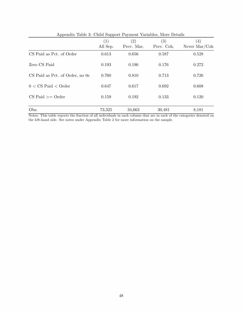
Appendix Table 3: Child Support Payment Variables, More Details(1) (2) (3) (4)

All Sep. Prev. Mar. Prev. Coh. Never Mar/Coh

CS Paid as Pct. of Order 0.613 0.656 0.587 0.528

Zero CS Paid 0.193 0.190 0.176 0.272

CS Paid as Pct. of Order, no 0s 0.760 0.810 0.713 0.726

0 < CS Paid < Order 0.647 0.617 0.692 0.608

CS Paid >= Order 0.159 0.192 0.133 0.120

Obs. 73,325 34,663 30,481 8,181Notes: This table reports the fraction of all individuals in each column that are in each of the categories denoted onthe left-hand side. See notes under Appendix Table 2 for more information on the sample.

48

Page 50

Appendix Table 4: Effect of Average Child Support Orders on Average Child Support Paid in theYears After Separation, Different Polynomial Specifications

Dep. Var.: Average Child Support Paid in Years After Sep.

(1) (2) (3) (4) (5)Poly 1 Poly 2 Poly 3 Poly 4 20K Bins

Average child 0.262∗∗∗ 0.365∗∗∗ 0.364∗∗∗ 0.400∗∗∗ 0.427∗∗∗support order after sep. [0.0154] [0.0253] [0.0260] [0.0304] [0.0317]

Dad inc. at sep. 0.0149∗∗∗ 0.00550 -0.0163 0.372[0.00158] [0.00956] [0.0530] [0.254]

Dad inc. squared 0.0000111 0.0000774 -0.00181[0.0000160] [0.000173] [0.00125]

Dad inc. cubed -6.39e-08 0.00000388[0.000000181] [0.00000264]

Dad inc. quartic -2.98e-09[2.03e-09]

Mean, dept. var. 9.252 9.252 9.252 9.252 9.252Obs. 70639 70639 70639 70639 70639R-squared 0.314 0.315 0.315 0.315 0.317Notes: All income variables are in year 2000 real units of 1,000 DKK. See notes under Appendix Table 2 and Table3 for more information on the sample and controls. The following functions of the father’s real income in the yearof separation are included: column 1 — linear polynomial, column 2 — quadratic polynomial, column 3 — cubicpolynomial, column 4 — quartic polynomial, column 5 — indicators for 20,000 DKK bins. All regressions include thecontrols listed in the notes under Table 3 as well as a full set of fixed effects and interactions for number of children,year of separation, and the interactions between them and the father’s income function. Additionally, the regressionsinclude indicators for the number of children still under age 18 in each year post-separation that the parents had (notincluding any new children born post-separation). Standard errors robust to heteroskedasticity.Significance levels: * p<0.1 ** p<0.05 *** p<0.01

49

Page 51

Appendix Table 5: Effect of Average Child Support Orders on the Incidence of Fathers Ever Livingwith Their Children After Separation, Different Polynomial Specifications

Dep. Var.: Father Ever Lives w/ Child After Sep.

(1) (2) (3) (4) (5)Poly 1 Poly 2 Poly 3 Poly 4 20K Bins

Average child -0.000987 -0.00477∗∗∗ -0.00403∗∗∗ -0.00565∗∗∗ -0.00494∗∗∗support order after sep. [0.000731] [0.00129] [0.00136] [0.00167] [0.00171]

Dad inc. at sep. -0.000151∗ -0.000298 -0.00151 -0.0127[0.0000823] [0.000559] [0.00310] [0.0149]

Dad inc. squared 0.000000373 0.00000427 0.0000594[0.000000872] [0.00000979] [0.0000712]

Dad inc. cubed -4.07e-09 -0.000000120[9.91e-09] [0.000000147]

Dad inc. quartic 8.86e-11[1.10e-10]

Mean, dept. var. 0.278 0.278 0.278 0.278 0.278Obs. 70639 70639 70639 70639 70639R-squared 0.0759 0.0762 0.0765 0.0767 0.0783Notes: All income variables are in year 2000 real units of 1,000 DKK. See notes under Appendix Table 2 and Table3 for more information on the sample and controls. The following functions of the father’s real income in the yearof separation are included: column 1 — linear polynomial, column 2 — quadratic polynomial, column 3 — cubicpolynomial, column 4 — quartic polynomial, column 5 — indicators for 20,000 DKK bins. All regressions include thecontrols listed in the notes under Table 3 as well as a full set of fixed effects and interactions for number of children,year of separation, and the interactions between them and the father’s income function. Additionally, the regressionsinclude indicators for the number of children still under age 18 in each year post-separation that the parents had (notincluding any new children born post-separation). Standard errors robust to heteroskedasticity.Significance levels: * p<0.1 ** p<0.05 *** p<0.01

50

Page 52

Appendix Table 6: Effect of Average Child Support Orders on Average Child Support Paid in theYears After Separation, Different Bin Specifications

Dep. Var.: Average Child Support Paid in Years After Sep.

(1) (2) (3) (4) (5)50K Bins 25K Bins 20K Bins 15K Bins 10K Bins

Average child 0.405∗∗∗ 0.428∗∗∗ 0.427∗∗∗ 0.436∗∗∗ 0.450∗∗∗support order after sep. [0.0268] [0.0309] [0.0317] [0.0324] [0.0334]

Mean, dept. var. 9.252 9.252 9.252 9.252 9.252Obs. 70639 70639 70639 70639 70639R-squared 0.315 0.317 0.317 0.318 0.320Notes: All income variables are in year 2000 real units of 1,000 DKK. See notes under Appendix Table 2 and Table3 for more information on the sample and controls. The following functions of the father’s real income in the year ofseparation are included: column 1 — indicators for 50,000 DKK bins, column 2 — indicators for 25,000 DKK bins,column 3 — indicators for 20,000 DKK bins, column 4 — indicators for 15,000 DKK bins, column 5 — indicatorsfor 10,000 DKK bins. All regressions include the controls listed in the notes under Table 3 as well as a full set offixed effects and interactions for number of children, year of separation, and the interactions between them and thefather’s income function. Additionally, the regressions include indicators for the number of children still under age 18in each year post-separation that the parents had (not including any new children born post-separation). Standarderrors robust to heteroskedasticity.Significance levels: * p<0.1 ** p<0.05 *** p<0.01

51

Page 53

Appendix Table 7: Effect of Average Child Support Orders on the Incidence of Fathers Ever Livingwith Their Children After Separation, Different Bin Specifications

Dep. Var.: Father Ever Lives w/ Child After Sep.

(1) (2) (3) (4) (5)50K Bins 25K Bins 20K Bins 15K Bins 10K Bins

Average child -0.00364∗∗∗ -0.00485∗∗∗ -0.00494∗∗∗ -0.00631∗∗∗ -0.00531∗∗∗support order after sep. [0.00130] [0.00164] [0.00171] [0.00178] [0.00183]

Mean, dept. var. 0.278 0.278 0.278 0.278 0.278Obs. 70639 70639 70639 70639 70639R-squared 0.0770 0.0779 0.0783 0.0789 0.0805Notes: All income variables are in year 2000 real units of 1,000 DKK. See notes under Appendix Table 2 and Table3 for more information on the sample and controls. The following functions of the father’s real income in the year ofseparation are included: column 1 — indicators for 50,000 DKK bins, column 2 — indicators for 25,000 DKK bins,column 3 — indicators for 20,000 DKK bins, column 4 — indicators for 15,000 DKK bins, column 5 — indicatorsfor 10,000 DKK bins. All regressions include the controls listed in the notes under Table 3 as well as a full set offixed effects and interactions for number of children, year of separation, and the interactions between them and thefather’s income function. Additionally, the regressions include indicators for the number of children still under age 18in each year post-separation that the parents had (not including any new children born post-separation). Standarderrors robust to heteroskedasticity.Significance levels: * p<0.1 ** p<0.05 *** p<0.01

52

Page 54

Appendix Table 8: Effect of Average Child Support Orders on Average Child Support Paid in theYears After Separation, Different Windows

Dep. Var.: Average Child Support Paid in Years After Sep.

(1) (2) (3) (4) (5)20K 40K 60K 80K 100K

Average child 0.498∗∗∗ 0.461∗∗∗ 0.429∗∗∗ 0.433∗∗∗ 0.427∗∗∗support order after sep. [0.0430] [0.0374] [0.0346] [0.0330] [0.0317]

Mean, dept. var. 9.369 9.357 9.320 9.302 9.252Obs. 45585 54002 60634 66002 70639R-squared 0.307 0.313 0.314 0.316 0.317Notes: All income variables are in year 2000 real units of 1,000 DKK. See notes under Appendix Table 2 and Table 3for more information on the sample, specifications, and controls. Samples of analysis are chosen based on the followingincome windows surrounding the first three thresholds: column 1 — 20,000 DKK, column 2 — 40,000 DKK, column3 — 60,000 DKK, column 4 — 80,000 DKK column 5 — 100,000 DKK. Standard errors robust to heteroskedasticity.Significance levels: * p<0.1 ** p<0.05 *** p<0.01

53

Page 55

Appendix Table 9: Effect of Average Child Support Orders on the Incidence of Fathers Ever Livingwith Their Children After Separation, Different Windows

Dep. Var.: Father Ever Lives w/ Child After Sep.

(1) (2) (3) (4) (5)20K 40K 60K 80K 100K

Average child -0.00396 -0.00317 -0.00288 -0.00418∗∗ -0.00494∗∗∗support order after sep. [0.00267] [0.00229] [0.00204] [0.00187] [0.00171]

Mean, dept. var. 0.277 0.278 0.278 0.278 0.278Obs. 45585 54002 60634 66002 70639R-squared 0.0765 0.0773 0.0781 0.0789 0.0783Notes: All income variables are in year 2000 real units of 1,000 DKK. See notes under Appendix Table 2 and Table 3for more information on the sample, specifications, and controls. Samples of analysis are chosen based on the followingincome windows surrounding the first three thresholds: column 1 — 20,000 DKK, column 2 — 40,000 DKK, column3 — 60,000 DKK, column 4 — 80,000 DKK column 5 — 100,000 DKK. Standard errors robust to heteroskedasticity.Significance levels: * p<0.1 ** p<0.05 *** p<0.01

54

Page 56

Appendix Table 10: Effect of Average Child Support Orders on the Likelihood of Mothers HavingChildren After Separation, Different Polynomial Specifications

Dep. Var.: Mother Has More Kids in Years After Sep.

(1) (2) (3) (4) (5)Poly 1 Poly 2 Poly 3 Poly 4 20K Bins

Average child 0.000799 0.00287∗∗∗ 0.00293∗∗∗ 0.00505∗∗∗ 0.00505∗∗∗support order after sep. [0.000543] [0.000787] [0.000812] [0.000857] [0.000844]

Dad inc. at sep. -0.0000799 -0.000521 -0.00166 -0.0178[0.0000702] [0.000482] [0.00267] [0.0130]

Dad inc. squared 0.000000554 0.00000411 0.0000832[0.000000734] [0.00000834] [0.0000615]

Dad inc. cubed -3.53e-09 -0.000000170[8.37e-09] [0.000000126]

Dad inc. quartic 1.27e-10[9.37e-11]

Mean, dept. var. 0.185 0.185 0.185 0.185 0.185Obs. 68941 68941 68941 68941 68941R-squared 0.213 0.213 0.213 0.213 0.215Notes: All income variables are in year 2000 real units of 1,000 DKK. See notes under Appendix Table 2 and Table3 for more information on the sample and controls. The following functions of the father’s real income in the yearof separation are included: column 1 — linear polynomial, column 2 — quadratic polynomial, column 3 — cubicpolynomial, column 4 — quartic polynomial, column 5 — indicators for 20,000 DKK bins. All regressions include thecontrols listed in the notes under Table 3 as well as a full set of fixed effects and interactions for number of children,year of separation, and the interactions between them and the father’s income function. Additionally, the regressionsinclude indicators for the number of children still under age 18 in each year post-separation that the parents had (notincluding any new children born post-separation). Standard errors robust to heteroskedasticity.Significance levels: * p<0.1 ** p<0.05 *** p<0.01

55

Page 57

Appendix Table 11: Effect of Average Child Support Orders on the Likelihood of Fathers HavingChildren After Separation, Different Polynomial Specifications

Dep. Var.: Father Has More Kids in Years After Sep.

(1) (2) (3) (4) (5)Poly 1 Poly 2 Poly 3 Poly 4 20K Bins

Average child 0.000386 0.00272∗∗∗ 0.00243∗∗∗ 0.00569∗∗∗ 0.00582∗∗∗support order after sep. [0.000577] [0.000912] [0.000934] [0.00101] [0.00102]

Dad inc. at sep. 0.000181∗∗ 0.000202 -0.00431 0.00282[0.0000763] [0.000520] [0.00288] [0.0139]

Dad inc. squared -0.000000174 0.0000143 -0.0000194[0.000000801] [0.00000904] [0.0000662]

Dad inc. cubed -1.47e-08 5.32e-08[9.11e-09] [0.000000136]

Dad inc. quartic -5.00e-11[1.01e-10]

Mean, dept. var. 0.186 0.186 0.186 0.186 0.186Obs. 70639 70639 70639 70639 70639R-squared 0.140 0.140 0.140 0.141 0.143Notes: All income variables are in year 2000 real units of 1,000 DKK. See notes under Appendix Table 2 and Table3 for more information on the sample and controls. The following functions of the father’s real income in the yearof separation are included: column 1 — linear polynomial, column 2 — quadratic polynomial, column 3 — cubicpolynomial, column 4 — quartic polynomial, column 5 — indicators for 20,000 DKK bins. All regressions include thecontrols listed in the notes under Table 3 as well as a full set of fixed effects and interactions for number of children,year of separation, and the interactions between them and the father’s income function. Additionally, the regressionsinclude indicators for the number of children still under age 18 in each year post-separation that the parents had (notincluding any new children born post-separation). Standard errors robust to heteroskedasticity.Significance levels: * p<0.1 ** p<0.05 *** p<0.01

56

Page 58

Appendix Table 12: Effects of Average Child Support Orders on Mothers’ Post-Separation LaborMarket Outcomes

(1) (2) (3) (4) (5)Any Wage Log Wage Emp. Self-Emp. NILF

Average child 0.000723 0.00734∗ 0.00102 0.000335 0.000561support order after sep. [0.000860] [0.00387] [0.000998] [0.000498] [0.000699]

Mean, dept. var. 0.847 11.82 0.753 0.0237 0.0691Obs. 68869 65525 68941 68941 68941Notes: The outcomes are defined as follows: 1) “Any Wage” refers to the proportion of years the mother has any wageincome post-separation, 2) “Log Wage” refers to the log of the mother’s average annual wage income in the yearspost-separation, 3) “Emp.” refers to the proportion of years the mother is employed in the private or public sector(not self-employed) post-separation, 4) “Self-Emp.” refers to the proportion of years the mother is self-employedpost-separation, and 5) “NILF” refers to the proportion of years the mother is not in the labor force post-separation.All income variables are in year 2000 real units of 1,000 DKK. See notes under Tables 2 and 3 for more informationon the sample, specifications, and controls. Standard errors robust to heteroskedasticity.Significance levels: * p<0.1 ** p<0.05 *** p<0.01

57

Page 59

Appendix Table 13: Effect of Average Child Support Orders on the Fraction of Years Fathers areNot in the Labor Force After Separation, Different Polynomial Specifications

Dep. Var.: Proportion of Time NILF in Years After Sep.

(1) (2) (3) (4) (5)Poly 1 Poly 2 Poly 3 Poly 4 20K Bins

Average child 0.00626∗∗∗ 0.000439 -0.000513 0.00204∗∗∗ 0.00176∗∗∗support order after sep. [0.000241] [0.000359] [0.000383] [0.000477] [0.000458]

Dad inc. at sep. -0.000406∗∗∗ -0.00143∗∗∗ -0.00415∗∗∗ -0.00684[0.0000250] [0.000171] [0.000928] [0.00450]

Dad inc. squared 0.00000192∗∗∗ 0.0000106∗∗∗ 0.0000249[0.000000254] [0.00000280] [0.0000208]

Dad inc. cubed -8.68e-09∗∗∗ -4.15e-08[2.72e-09] [4.15e-08]

Dad inc. quartic 2.65e-11[3.02e-11]

Mean, dept. var. 0.0418 0.0418 0.0418 0.0418 0.0418Obs. 70639 70639 70639 70639 70639R-squared 0.0941 0.102 0.107 0.109 0.109Notes: All income variables are in year 2000 real units of 1,000 DKK. See notes under Appendix Table 2 and Table3 for more information on the sample and controls. The following functions of the father’s real income in the yearof separation are included: column 1 — linear polynomial, column 2 — quadratic polynomial, column 3 — cubicpolynomial, column 4 — quartic polynomial, column 5 — indicators for 20,000 DKK bins. All regressions include thecontrols listed in the notes under Table 3 as well as a full set of fixed effects and interactions for number of children,year of separation, and the interactions between them and the father’s income function. Additionally, the regressionsinclude indicators for the number of children still under age 18 in each year post-separation that the parents had (notincluding any new children born post-separation). Standard errors robust to heteroskedasticity.Significance levels: * p<0.1 ** p<0.05 *** p<0.01

58

Page 60

App

endixTa

ble14

:Eff

ects

ofEx

pected

Saving

sin

Child

Supp

ortObligations

from

Havingan

IncomeBelow

the1stThresho

ldon

Fathers’

Post-Sep

arationLa

borMarketOutcomes

(1)

(2)

(3)

(4)

(5)

(6)

(7)

(8)

Any

Wag

eLo

gWag

eEm

p.Se

lf-Em

p.NILF

Dis.

Welf.

Ret.

Valueof

mov

ing

-0.007

63∗∗

-0.006

21-0.005

33-0.001

130.01

01∗∗∗

0.00

531∗∗∗

-0.000

235

0.00

556∗∗∗

below

thres.

1as

pctof

income

[0.003

77]

[0.018

5][0.004

54]

[0.003

91]

[0.002

00]

[0.001

31]

[0.001

14]

[0.001

06]

Mean,

dept.var.

0.91

512

.26

0.83

20.06

110.04

180.01

130.02

490.00

364

Obs.

7062

669

184

7063

970

639

7063

970

639

7063

970

639

Notes:Thistablepresents

results

from

regression

swhe

rethekeyexplan

atoryvaria

bleis

theaveragean

nual

real

saving

sin

child

supp

ortob

ligations,as

ape

rcentage

ofthefather’ssepa

ratio

nyear

real

income,

that

wou

ldaccrue

ifthefather

hadan

incomebe

low

the1stgu

idelinethreshold.

Thisvaria

bleisexpressed

inpe

rcentage

pointun

its.The

outcom

esarede

fined

asfollo

ws:

1)“A

nyWage”

refers

totheprop

ortio

nof

yearsthefather

hasan

ywageincomepo

st-sep

aration,

2)“L

ogWage”

refers

tothelogof

thefather’s

averagean

nual

wageincomein

theyearspo

st-sep

aration,

3)“E

mp.”

refers

totheprop

ortio

nof

yearsthefather

isem

ployed

intheprivateor

public

sector

(not

self-em

ployed

)po

st-sep

aration,

4)“S

elf-E

mp.”

refers

totheprop

ortio

nof

yearsthefather

isself-em

ployed

post-separation,

5)“N

ILF”

refers

totheprop

ortio

nof

yearsthefather

isno

tin

thelabo

rforcepo

st-sep

aration,

6)“D

is.”

refers

totheprop

ortio

nof

yearsthe

father

isno

tin

thelabo

rforcedu

eto

disabilityleavepo

st-sep

aration,

7)“W

elf.”

refers

totheprop

ortio

nof

yearsthefather

isno

tin

thelabo

rforcean

dreceiving

welfare

bene

fits,an

d8)

“Ret.”

refers

totheprop

ortio

nof

yearsthefather

isno

tin

thelabo

rforcedu

eto

retir

ement(in

clud

ingearly

retir

ement)

post-sep

aration.

Allincomevaria

bles

arein

year

2000

real

units

of1,000DKK.S

eeno

tesun

derApp

endixTa

ble2an

dTa

ble3formoreinform

ationon

thesample,

specificatio

ns,

andcontrols.Stan

dard

errors

robu

stto

heterosked

astic

ity.

Sign

ificancelevels:*p<

0.1**

p<0.05

***p<

0.01

59

Page 61

Appendix Table 15: Instrumental Variables Results(1) (2) (3) (4) (5)

Avg. CS Paid F. Live w/Child F. More Kids M. More Kids F. NILF

Average child 0.507∗∗∗ -0.00594∗∗∗ 0.00692∗∗∗ 0.00600∗∗∗ 0.00209∗∗∗support order, using [0.0369] [0.00203] [0.00116] [0.000997] [0.000547]current inc. and num kids

Mean, dept. var. 9.251 0.278 0.186 0.185 0.0418Fst. stage coef. 0.841 0.841 0.841 0.843 0.841Fst. stage F-stat 2619.5 2619.5 2619.5 2612.7 2619.5Obs. 70637 70637 70637 68940 70637Notes: “F.” refers to fathers’ outcomes, while “M.” refers to mothers’ outcomes. In these specifications, we cal-culate child support obligations based on fathers’ actual current incomes and numbers of children in each yearpost-separation, and then use our main treatment variable (based on income and number of children in the yearof separation) as an instrument. All income variables are in year 2000 real units of 1,000 DKK. See notes underAppendix Table 2 and Table 3 for more information on the sample, specifications, and controls. Standard errorsrobust to heteroskedasticity.Significance levels: * p<0.1 ** p<0.05 *** p<0.01

60

Page 62

Appendix Table 16: Results Using Father’s Income in Year Before Separation to Calculate ChildSupport Obligations

(1) (2) (3) (4) (5)Avg. CS Paid F. Live w/Child F. More Kids M. More Kids F. NILF

Average child 0.469∗∗∗ -0.00312∗ 0.00837∗∗∗ 0.00599∗∗∗ 0.00162∗∗∗support order after sep. [0.0348] [0.00176] [0.00106] [0.000853] [0.000506]

Mean, dept. var. 9.452 0.278 0.184 0.181 0.0435Obs. 70532 70532 70532 68910 70532Notes: “F.” refers to fathers’ outcomes, while “M.” refers to mothers’ outcomes. The results reported here are fromspecifications where child support obligations are assigned based on the father’s income measured in the year beforeseparation. All income variables are in year 2000 real units of 1,000 DKK. See notes under Appendix Table 2 andTable 3 for more information on the sample, specifications, and controls. Standard errors robust to heteroskedasticity.Significance levels: * p<0.1 ** p<0.05 *** p<0.01

61

Page 63

Appendix Table 17: Effects of Average Child Support Orders, 1-Child Families(1) (2) (3) (4) (5)

Avg. CS Paid F. Live w/Child F. More Kids M. More Kids F. NILF

Average child 0.333∗∗∗ -0.00219 0.00900∗∗∗ 0.0130∗∗∗ 0.00232∗∗∗support order after sep. [0.0368] [0.00240] [0.00144] [0.00120] [0.000766]

Mean, dept. var. 6.313 0.253 0.209 0.221 0.0470Obs. 39021 39021 39021 37466 39021Notes: “F.” refers to fathers’ outcomes, while “M.” refers to mothers’ outcomes. See notes under Appendix Table 2on the sample. Here, the sample is further limited to parents who had one child at the time of separation. All incomevariables are in year 2000 real units of 1,000 DKK. All regressions include fixed effects for 20,000 DKK bins in father’sincome and the year of separation. All regressions include controls (measured in the year of separation) for the father’sage and age squared, dummies for the father’s education (less than high school, high school, vocational/short-termhigher ed, college/university, and missing), an indicator for the father being from Western Europe, mother’s ageand age squared, dummies for the mother’s education (less than high school, high school, vocational/short-termhigher ed, college/university, and missing), an indicator for the mother being from Western Europe, mother’s totalincome in year 2000 DKK, the child’s age and age squared, and indicators for original parental relationship status(married, cohabiting, never-married/non-cohabiting). Additionally, the regressions include indicators for the numberof children still under age 18 in each year post-separation that the parents had (not including any new children bornpost-separation). Standard errors robust to heteroskedasticity.Significance levels: * p<0.1 ** p<0.05 *** p<0.01

62

Page 64

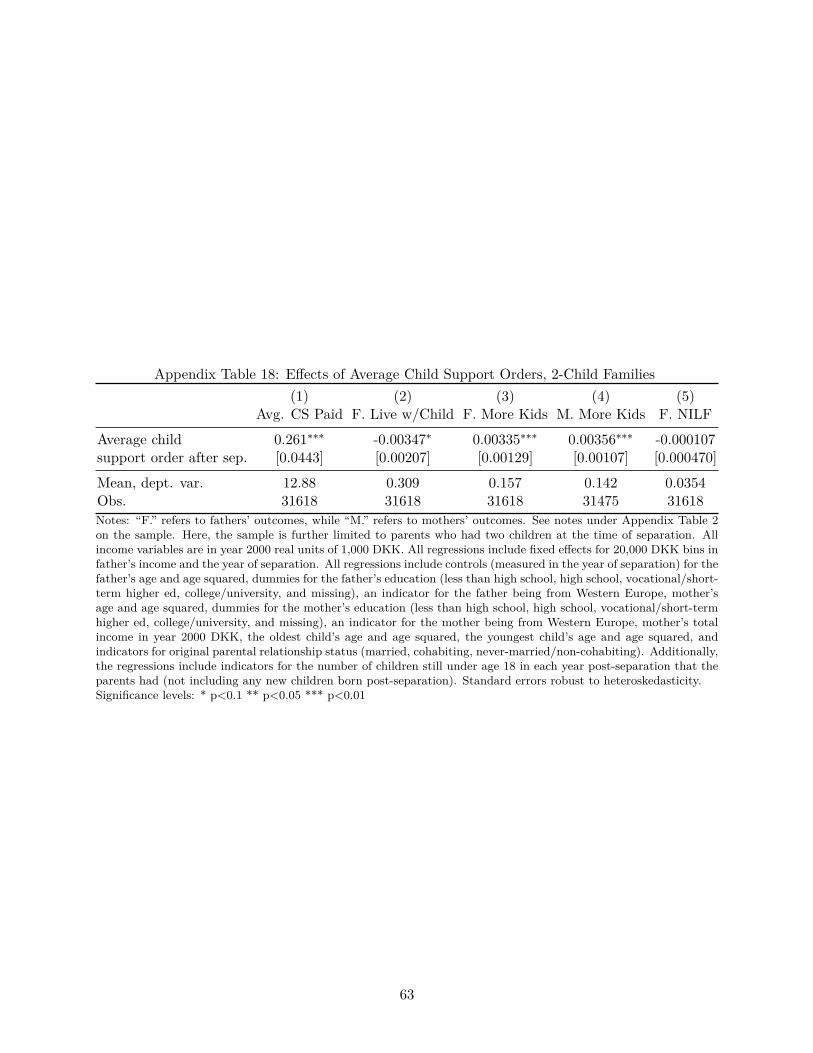
Appendix Table 18: Effects of Average Child Support Orders, 2-Child Families(1) (2) (3) (4) (5)

Avg. CS Paid F. Live w/Child F. More Kids M. More Kids F. NILF

Average child 0.261∗∗∗ -0.00347∗ 0.00335∗∗∗ 0.00356∗∗∗ -0.000107support order after sep. [0.0443] [0.00207] [0.00129] [0.00107] [0.000470]

Mean, dept. var. 12.88 0.309 0.157 0.142 0.0354Obs. 31618 31618 31618 31475 31618Notes: “F.” refers to fathers’ outcomes, while “M.” refers to mothers’ outcomes. See notes under Appendix Table 2on the sample. Here, the sample is further limited to parents who had two children at the time of separation. Allincome variables are in year 2000 real units of 1,000 DKK. All regressions include fixed effects for 20,000 DKK bins infather’s income and the year of separation. All regressions include controls (measured in the year of separation) for thefather’s age and age squared, dummies for the father’s education (less than high school, high school, vocational/short-term higher ed, college/university, and missing), an indicator for the father being from Western Europe, mother’sage and age squared, dummies for the mother’s education (less than high school, high school, vocational/short-termhigher ed, college/university, and missing), an indicator for the mother being from Western Europe, mother’s totalincome in year 2000 DKK, the oldest child’s age and age squared, the youngest child’s age and age squared, andindicators for original parental relationship status (married, cohabiting, never-married/non-cohabiting). Additionally,the regressions include indicators for the number of children still under age 18 in each year post-separation that theparents had (not including any new children born post-separation). Standard errors robust to heteroskedasticity.Significance levels: * p<0.1 ** p<0.05 *** p<0.01

63

Page 65

B Evidence on Custody Arrangements from Survey Data

In Section 4, we argue that an important factor driving the zero payments we observe in our data

is joint physical custody arrangements. Unfortunately, the administrative data we use contain an

imperfect measure of physical custody based on whether the child is registered at the same address

as the parent. As children can only have one address in our data (irrespective of their custody

arrangement), we underestimate joint physical custody arrangements by looking at children who

are registered at the same address as their fathers.

To further examine the relationship between physical custody arrangements and child support

payments, we link our administrative data to survey data from Denmark. As sample sizes for

children living in non-intact families in available surveys are small, we pool data from two sources:

first, the 2007 wave of the Danish longitudinal survey of children (DALSC), and second, the 2009

wave of the Children and Youth in Denmark (CYD) survey.46 The DALSC is a panel study of all

children born in Denmark in one week of October 1995. The CYD is a survey conducted among

random samples of seven cohorts aged 3-19 in 2009 and 2013. Both panel studies examine a broad

set of topics related to children’s living conditions, including custody arrangements.

We link the survey information to the administrative data on child support payments. Similar

to our sample construction described in Section 4, we keep children whose fathers are in the admin-

istrative data in all years after 1995 (the initiation year of the DALSC). We match 5, 738 DALSC

and 5, 988 CYU children to the administrative data (99/95% of the children with completed survey

questionnaires). In 2007, the DALSC children were 12 years old and thus we have a relatively large

share of children who have experienced a parental separation: After conditioning on the fathers

being in the data for all years after 1995 and experiencing a separation at any time during the

period, we end up with 2, 024 separated fathers with (singleton) children. For the CYD data, we

end up with 1, 428 fathers.

As we use parental reports on physical custody arrangements (the vast majority of question-

naires were completed by mothers), we further condition on the parents having answered ques-

tions on the custody arrangements (i.e., separated before the surveys in 2007/2009). Finally, we

only look at one- and two-children families with fathers in the relevant income range (around the

guideline thresholds), as in the main analysis. Our final survey sample consists of parents of 843

(DALSC)/765 (CYD) children.

Appendix Table 19 divides this sample of children into three groups: Column 1 reports summary46For details on the DALSC and CYU please see http://www.sfi.dk/about_the_research-11402.aspx and

http://www.sfi.dk/children_and_young_people_in_denmark-7395.aspx.

64

Page 66

statistics for the full survey sample of separated parents. Columns 2 and 3 show summary statistics

for the two sub-groups: children with sole-mother and children with either joint or sole-father

physical custody arrangements as reported in the respective survey years (2007 for DALSC and

2009 for CYD). Joint physical custody is defined as the child spending approximately half of the

time with each parent (in the survey year). Given that we only have 49 fathers with sole physical

custody in our data, and as paternal child support obligations do not apply to both joint and sole

physical custody fathers, we pool the two groups.

In the top panel, we report means and standard deviations of some of the child support variables

from the administrative data. While our main analysis focuses on fathers’ child support obligations

and payments, we also describe maternal child support payments here as they are especially relevant

for the joint and sole-father physical custody arrangements.

We find that fathers who share in the physical custody in the survey year (and especially if they

have sole custody) pay less child support over the separation time relative to fathers who do not.

The percentage of fathers with zero payments is higher among fathers who have sole or joint physical

custody in the survey year: 46 percent of sole- or joint-custody fathers make zero payments in that

year (relative to 35 percent of fathers whose children live in sole-mother custody arrangements).

These figures illustrate that a large share of the zeros we observe in our administrative data is likely

driven by fathers who share in physical custody of their children.

Additionally, while the 21 percent of fathers with joint or sole physical custody in the survey

year pay less than their non-custody counterparts, the survey data also show that mothers pay more

in these cases: Mothers of children in sole-father or joint physical custody arrangements pay more

than four times as much as sole-custody mothers, and are less likely to ever have zero payments

after separation. However, the relatively low level of average post-separation mother payments

reflects that mothers are most likely to have physical custody of their children in some (if not all)

of the pre-survey separation years.

The last row in the top panel shows that our measure of father-child co-residence—an indicator

for the father having the same address as the child in any year post-separation—is reasonable

(although imperfect). Fathers who have joint or sole physical custody are more likely to be registered

at the same address as their child relative to fathers of children in sole-mother custody arrangements.

Finally, the lower panel focuses on a variable only available in the DALSC data. We look at our

2007 DALSC sample of parents and their reports from any of the survey years (1996, 1999, 2003,

2007, 2011). These data show that joint physical custody arrangements are relatively fluid over

separation time: among parents who have a sole-mother arrangement in 2007, 13 percent have joint

65

Page 67

custody in any of the survey years. Overall, 33 percent of parents have a joint custody arrangement

in at least one of the survey years.

In sum, using the available survey data (linked to our administrative data), we find that joint

(and sole-father) physical custody arrangements (which we underestimate when using only ad-

ministrative data on addresses) coincide with lower average father child support payments, higher

prevalence of zero payments by fathers, and higher average mother payments. Moreover, as around

33 percent of parents have a joint physical custody arrangement at some point post-separation,

and as parents sharing physical custody do not face child support mandates, we conclude that a

large percentage of the observed zero-payments in our main analysis data set is attributable to the

prevalence of these arrangements.

66

Page 68

Appendix Table 19: Physical Custody Arrangements and Child Support Payments: Evidence fromAdministrative Data Linked to Survey Data from 2007 (DALSC) and 2009 (CYD)

DALSC and CYD samples, admin. data

(1) (2) (3)All parents Sole-Mother Joint and Sole-Father

Father: Child support payments in 11298.4 11666.8 9893.0survey year (12099.7) (12237.5) (11468.1)

Father: Zero 0.368 0.345 0.455child support in survey year (0.482) (0.476) (0.499)

Father: Average 11398.0 11846.5 9687.1child support paid after sep. (9746.5) (9697.4) (9758.0)

Father: Ever zero 0.704 0.684 0.781child support after sep. (0.457) (0.465) (0.414)

Father: Always zero 0.160 0.141 0.237child support after sep. (0.367) (0.348) (0.426)

Father: Average 21750.6 21438.9 22941.2child support order after sep. (9440.8) (9321.1) (9808.2)

Mother: Average 1035.9 599.8 2699.4child support paid after sep. (3210.9) (2330.9) (5047.6)

Mother: Ever zero 0.973 0.986 0.922child support after sep. (0.163) (0.118) (0.268)

Father: Ever lives 0.249 0.239 0.287with the child after sep. (0.433) (0.427) (0.453)

Obs. 1,608 1,274 334Survey data, DALSC

(1) (2) (3)

Joint physical 0.325 0.130 0.840custody, any survey year (0.469) (0.336) (0.367)

Obs. 843 618 225Notes: Columns 2-4 divide the sample by the physical custody arrangement (sole-mother, sole-father, joint) in thesurvey year (2007/2009).

67