Welcome message from author
This document is posted to help you gain knowledge. Please leave a comment to let me know what you think about it! Share it to your friends and learn new things together.
Transcript

Impressum
Copyright © 2020 by CEPOS InSilico GmbH
Waldstraße 15
90587 Obermichelbach
Germany
www.ceposinsilico.com
Manual Timothy Clark
Layout www.eh-bitartist.de

TABLE OF CONTENTS
ParaSurf20 Users´ Manual
© CEPOS InSilico GmbH 2020
TABLE OF CONTENTS
PROGRAM HISTORY 5
1 INTRODUCTION 6 1.1 Changes relative to ParaSurf19™ 7
1.1.1 EMPIRE™ 7
1.2 Isodensity surfaces 7 1.3 Solvent-excluded surfaces 8 1.4 Solvent-accessible surfaces 8 1.5 Shrink-wrap surface algorithm 9 1.6 Marching-cube algorithm 10 1.7 Spherical-harmonic fitting 11 1.8 Local properties 13
1.8.1 Molecular electrostatic potential 13 1.8.1.1 The natural atomic orbital/PC (NAO-PC) model 13 1.8.1.2 The multipole model 13
1.8.2 Local ionization energy, electron affinity, hardness and electronegativity 13 1.8.3 Local polarizability 15 1.8.4 Field normal to the surface 15
1.9 Descriptors 16 1.10 Surface-integral models (polynomial version) 22 1.11 Binned surface-integral models 23 1.12 Spherical harmonic “hybrids” 24 1.13 Descriptors and moments based on polynomial surface-integral models 25 1.14 Shannon entropy 26 1.15 Surface autocorrelations 28 1.16 Standard rotationally invariant fingerprints (RIFs) 30 1.17 Maxima and minima of the local properties 30 1.18 Atom-centred descriptors 30 1.19 Fragment analysis 30
2 PROGRAM OPTIONS 31 2.1 Command-line options 31 2.2 Options defined in the input SDF-file 36
2.2.1 Defining the centre for spherical-harmonic fits 36 2.2.2 Defining fragments 37
3 INPUT AND OUTPUT FILES 41 3.1 EMPIRE™HDF5 (*e.h5) output files 42 3.2 The EMPIRE™ or VAMP .sdf files as input 42
3.2.1 Multi-structure SD-files 45
3.3 The Cepos MOPAC 6.sdf file as input 45 3.4 The <Hamiltonian>.par file 45 3.5 The EMPIRE™ binary wavefunction file (.vwf) 46 3.6 The ParaSurf™ output file 47
3.6.1 For a spherical-harmonic surface 47

TABLE OF CONTENTS
ParaSurf20 Users´ Manual
© CEPOS InSilico GmbH 2020
3.6.2 For a marching-cube surface 55 3.6.3 For a job with Shannon entropy 61 3.6.4 For a job with autocorrelation similarity 62
3.7 ParaSurf™ SDF-output 63 3.7.1 Optional blocks in the SDF-output file 66
3.8 The surface (.psf) file 69 3.9 Anonymous SD (.asd) files 70
3.9.1 Optional blocks 71
3.10 Grid calculations with ParaSurf™ 72 3.10.1 User-specified Grid 72 3.10.2 Automatic grids 73
3.11 The SIM file format 74 3.12 Output tables 76 3.13 Binned SIM descriptor tables 80 3.14 Autocorrelation fingerprint and similarity tables 81 3.15 Shared files 81
4 TIPS FOR USING PARASURF20™ 82 4.1 Choice of surface 82 4.2 Local properties 82 4.3 QSAR using grids 82
5 SUPPORT 83 5.1 Contact 83 5.2 Error reporting 83 5.3 CEPOS InSilico GmbH 83
6 LIST OF TABLES 84
7 LIST OF FIGURES 85
8 REFERENCES 86

PROGRAM HISTORY
ParaSurf20 Users´ Manual
© CEPOS InSilico GmbH 2020
PROGRAM HISTORY
Release Date Version Platforms
1st July 2005 ParaSurf´05™ initial release(Revision A1) 32-bit Windows
32-bit Linux
Irix 1st January 2006 ParaSurf´05™ Revision B1 (customer-feedback release)
1st July 2006 ParaSurf´06™ Revision A1 32-bit Windows
32-bit Linux
64-bit Linux
Irix 1st July 2007 ParaSurf´07™ Revision A1
1st July 2008 ParaSurf´08™ Revision A1
32-bit Windows
64-bit Windows
32-bit Linux
64-bit Linux
22nd August 2008 ParaSurf´08™ Revision A2 (minor bug fix release)
16th December 2008 ParaSurf´08™ Revision A3 (minor bug fix release)
1st July 2009 ParaSurf´09™ Revision A1
1st September 2009 New Vhamil.par file including PM6 and
first-row transition metals in AM1*
1st February 2010 ParaSurf´09™ Revision B1
(additional atom-centred descriptors)
1st July 2010 ParaSurf´10™ Revision A1
1st July 2011 ParaSurf´11™ Revision A1
1st September 2013 ParaSurf´12™ Revision A1
1st November 2019 ParaSurf19™ Revision A1 64-bit Windows
64-bit Linux
1st March 2020 ParaSurf19™ Revision A2
(Vhamil.par replaced by EMPIRE <Hamiltonian>.par file)
64-bit Windows
64-bit Linux
1st September 2020 ParaSurf20™ Revision A1 64-bit Windows
64-bit Linux

INTRODUCTION 6
ParaSurf20 Users´ Manual
© CEPOS InSilico GmbH 2020
1 INTRODUCTION
ParaSurf™ is a program to generate isodensity or solvent-excluded surfaces from the results of
semiempirical molecular orbital calculations, either from VAMP [1] or a public-domain version of MOPAC
modified and made available by Cepos InSilico.[2] The surface may be generated by shrink-wrap [3] or
marching-cube [4] algorithms and the former may be fit to a spherical harmonic series.[5] The principles
of these two techniques are explained below, but for comparison Figure 1 shows default isodensity
surfaces calculated by ParaSurf™ for a tetracycline derivative. The surfaces are color-coded according
to the electrostatic potential at the surface.
Figure 1 Marching-cube (left) and shrink-wrap (right, fitted to a spherical-harmonic approximation) isodensity surfaces calculated with
ParaSurf™ using the default settings
Four local properties, the molecular electrostatic potential (MEP),[6] the local ionization energy (IEL), [7]
the local electron affinity (EAL), [8] and the local polarizability (L) [8] are calculated at the points on the
surface. Two further properties, the local hardness (L), [8] and the local electronegativity (L) [8] can be
derived from IEL and EAL.
The local properties can be used to generate a standard set of 81 descriptors [9] appropriate for
quantitative structure-property relationships (QSPRs) for determining physical properties.
ParaSurf™ can also generate local enthalpies and free energies of solvation [10] and integrate them
over the entire molecular surface to give the enthalpy or free energy of solvation. ParaSurf™ can read
so-called Surface-Integral Model (SIM) files that allow it to calculate properties such as, for instance, the
enthalpy and free energy of hydration and the free energies of solvation in n-octanol and chloroform.
The surface-integral models are expressed as summations of local solvation energies over the
molecular surface. These local solvation energies can be written to the ParaSurf™ surface file.
ParaSurf™ is the first program to emerge from the ParaShift collaboration between researchers at the
Universities of Erlangen, Portsmouth, Southampton, Oxford and Aberdeen. It is intended to provide the
molecular surfaces for small molecules (i.e. non-proteins) for subsequent quantitative structure-activity
relationship (QSAR), QSPR, high-throughput virtual screening (HTVS), docking and scoring, pattern-
recognition and simulation software that will be developed in the ParaShift project.

INTRODUCTION 7
ParaSurf20 Users´ Manual
© CEPOS InSilico GmbH 2020
1.1 Changes relative to ParaSurf19™
The functionality of ParaSurf20™ has been extended to allow EMPIRE™ *_e.h5 binary HDF5 files to be
used as input. The naming of files for the input has also been made more flexible. In detail, the changes
relative to ParaSurf’19™ are:
• ParaSurf20™ now uses EMPIRE™ *_e.h5 file as the primary input format. The hierarchy of the input
file formats is defined below.
• ParaSurf20™ now accepts the full name of input files (e.g. molecule_e.h5, molecule_e.vwf or
molecule .sdf to enable the automatic hierarchy to be avoided.
• ParaSurf20™ accepts lists of files as input (see option inlist=<s>).
1.1.1 EMPIRE™
ParaSurf20™ is compatible with CeposInSilico’s EMPIRE20™ program for performing semiempirical
molecular orbital calculations and communicates with EMPIRE using the .h5 or .sdf file formats.
1.2 Isodensity surfaces
Isodensity surfaces [11] are defined as the surfaces around a molecule at which the electron density
has a constant value. Usually this value is chosen to approximate the van der Waals’ shape of the
molecule. ParaSurf™ allows values of the isodensity level down to 0.00001 e-Å-3. Lower values than this
may result in failures of the surface algorithms for very diffuse surfaces.
INTRODUCTION 8
ParaSurf20 Users´ Manual
© CEPOS InSilico GmbH 2020
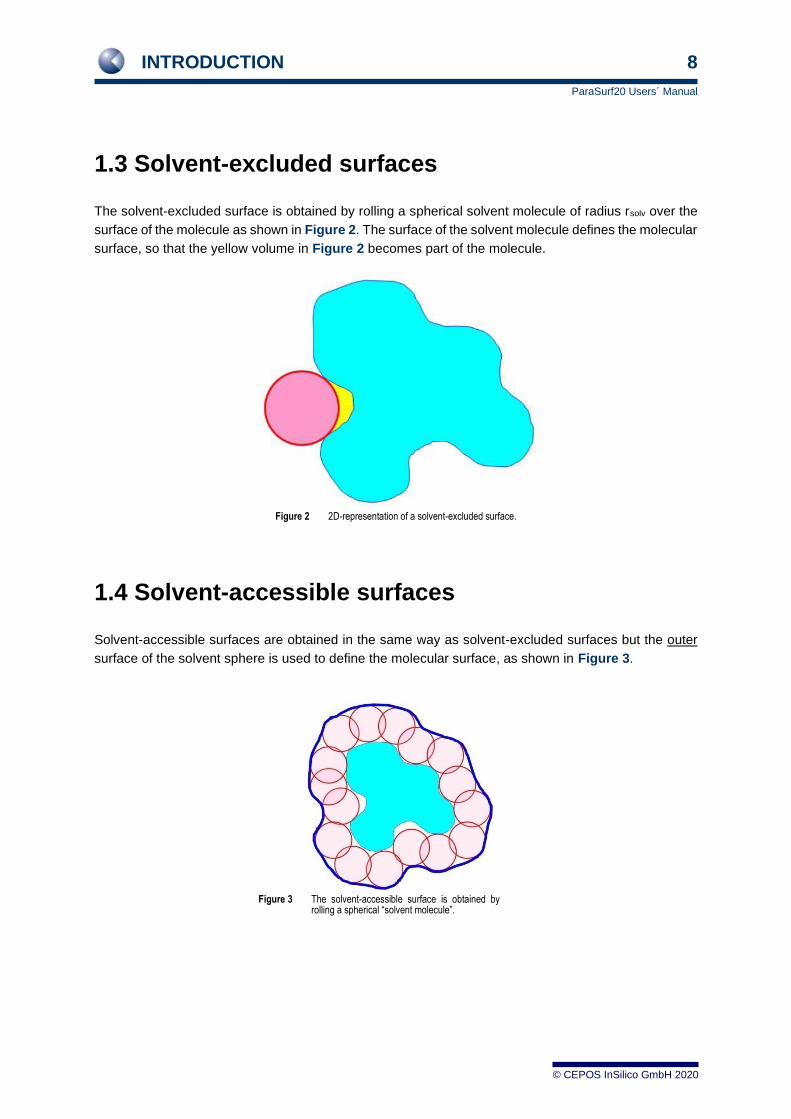
1.3 Solvent-excluded surfaces
The solvent-excluded surface is obtained by rolling a spherical solvent molecule of radius rsolv over the
surface of the molecule as shown in Figure 2. The surface of the solvent molecule defines the molecular
surface, so that the yellow volume in Figure 2 becomes part of the molecule.
Figure 2 2D-representation of a solvent-excluded surface.
1.4 Solvent-accessible surfaces
Solvent-accessible surfaces are obtained in the same way as solvent-excluded surfaces but the outer
surface of the solvent sphere is used to define the molecular surface, as shown in Figure 3.
Figure 3 The solvent-accessible surface is obtained by rolling a spherical “solvent molecule”.

INTRODUCTION 9
ParaSurf20 Users´ Manual
© CEPOS InSilico GmbH 2020
1.5 Shrink-wrap surface algorithm
Shrink-wrap surface algorithms [3] are used to determine single-valued molecular surfaces. Single-
valued in this case means that for any given radial vector from the centre of the molecule the surface is
only crossed once (vectors A and B in Figure 4) and not multiply (vectors C and D in Figure 4):
Figure 4 2D-representation of a molecular surface with single-valued (A and B) and multiply valued (C and D) radial vectors from the centre.
Single-valued surfaces are necessary for spherical-harmonic fitting (see Section 1.4). Thus, spherical-
harmonic fitting is only available for shrink-wrap surfaces in ParaSurf™. The shrink-wrap algorithm works
by starting outside the molecule (point a in Figure 5) and moving inwards along the radial vector until it
finds the surface (in our case defined by the predefined level of the electron density, point b in Figure
5). Thus, the shrink-wrapped surface may contain areas (marked by dashed lines in Figure 5) for which
the surface deviates from the true isodensity surface.
These areas of the surface, however, often have little consequence as they are situated above
indentations in the molecule that are poorly accessible to solvents or other molecules. The shrink-
wrapped surfaces generated by ParaSurf™ should normally be fitted to a spherical-harmonic series for
use in HTVS, similarity, pattern-recognition or high-throughput docking applications. The default
molecular centre in ParaSurf™ is the centre of gravity (CoG). In special cases in which the CoG lies
outside the molecule, another centre may be chosen.
Figure 5 2D-representation of the shrink-wrap algorithm. The algorithms scans along the vector from point a towards the centre of the molecule until the electron density reaches the preset value (point b). The algorithm results in enclosures (marked yellow) for multi-valued radial vectors.

INTRODUCTION 10
ParaSurf20 Users´ Manual
© CEPOS InSilico GmbH 2020
Figure 6 shows a spherical-harmonically fitted shrink-wrap surface for a difficult molecule. The areas
shown schematically in Figure 5 are clearly visible.
Figure 6 Spherical-harmonic approximation of a shrink-wrap isodensitiy surface. Note the areas where the surface does not follow the indentations of the molecule.
1.6 Marching-cube algorithm
The marching-cube algorithm [4] implemented in ParaSurf™ does not have the disadvantage of being
single-valued like the shrink-wrap surface. It cannot, therefore, be fitted to a spherical harmonic series
and is used as a purely numerical surface primarily for QSPR applications or surface-integral models.
[10] The algorithm works by testing the electron density at the corners of cubes on a cubic lattice laid
out through the molecular volume. The corners are divided into those “inside” the molecule (i.e. with a
higher electron density than the preset value) and those “outside”. The surface triangulation is then
generated for each surface cube and the positions of the surface points corrected to the preset electron
density.
INTRODUCTION 11
ParaSurf20 Users´ Manual
© CEPOS InSilico GmbH 2020
1.7 Spherical-harmonic fitting
Complex surfaces can be fitted to spherical harmonic series to give analytical approximations of the
surface.[5] The surfaces are fit to a series of distances from the centre along the radial vector
defined by the angles and as:
(1)
Where the distances are linear combinations of spherical harmonics Ylm
defined as:
(2)
where Pl
m (cos ) are associated Legendre functions and l and m are integers such that –l<=m<=l. In
the above form, spherical harmonics are complex functions. Duncan and Olson [12] have used the real
functions
(3)
where Nlm are normalization factors, to describe molecular surfaces using spherical harmonics.
ParaSurf™ not only fits the surface itself (i.e. the radial distances) to spherical harmonic expansions, but
also the four local properties (see Section 1.8). In this way, a completely analytical description of the
shape of the molecule and its intermolecular binding properties is obtained.[13] This description can be
truncated at different orders depending on the application and the precision needed. Thus, a simple
description of the molecular properties (shape, MEP, IEL, EAL and L) to order 2 consists of only five
sets of nine coefficients each, or 45 coefficients. These coefficients can be rotated, overlaps calculated
etc. [5] to give fast scanning of large numbers of compounds.
Note that, because of the approximate nature of the spherical-harmonic fits, the default isodensity level
for the shrink-wrapped surface (0.0005 e-Å-3) is lower than that (0.007 e-Å-3) appropriate for an
approximately van der Waals’ surface using the marching-cube algorithm. The lower value avoids the
surface coming too close to atoms. Note also that the fits are incremental, which means that the order
chosen for a given application can be obtained by ignoring coefficients of higher order in the spherical-
harmonic series.
In some cases, the default resolution of the molecular surface does not allow fitting the spherical-
harmonic expansion to very high orders without introducing noise (“ripples”) on the fitted surface. In this
case, the calculated RMSD becomes larger at higher orders of the spherical-harmonic expansion.
ParaSurf19™ recognizes this condition and truncates the fitting procedure at the optimum value. This
can be recognized in the output because the RMSD for later cycles remains constant and the coefficients
of the higher order spherical harmonics are all zero. This guarantees the optimum fit in each case and
is important for applications that use either the spherical-harmonic coefficients themselves or the
hybridization coefficients.
,r
,
0
N lm m
l l
l m l
r c Y
= =−
=
,r
(2 1)( )!( , ) (cos )
4 ( )!
m m im
l l
l l mY P e
l m
+ −=
+
( , ) (cos )cosm m
l lm lY N P m =
l
INTRODUCTION 12
ParaSurf20 Users´ Manual
© CEPOS InSilico GmbH 2020
The choice of centre for fitting to a spherical-harmonic expansion is critical. ParaSurf19™ therefore goes
through a multi-step procedure in order to find a suitable centre. This procedure is retained for all
molecules for which the ParaSurf’08™ found a suitable centre. However, if the algorithms implemented
in ParaSurf’08™ fail to find a suitable centre, the additional technique first implemented in ParaSurf’12™
will probably work.
The problem with many molecules is that, for instance, the centre of mass does not lie within the
molecular volume. This can easily be the case for, for instance, U- or L-shaped molecules. The
procedure implemented in ParaSurf19™ works as follows:
1. The program first calculates the centre of mass and tests whether it lies within the volume of
the molecule. If it does, it is used as the molecular centre. If not, the program moves on to the
next step.
2. ParaSurf™ calculates the principal moments of inertia of the molecule and derives a centre from
them by assuming that the molecule is U- or V-shaped. The procedure tries to place the centre
at the base centre of the molecule. This procedure was implemented in ParaSurf’08™ as a
fallback if the centre of mass proved unsuitable. If it also fails to find a suitable centre,
ParaSurf19™ moves on to a third option, which finds a centre for all but the most difficult
molecules.
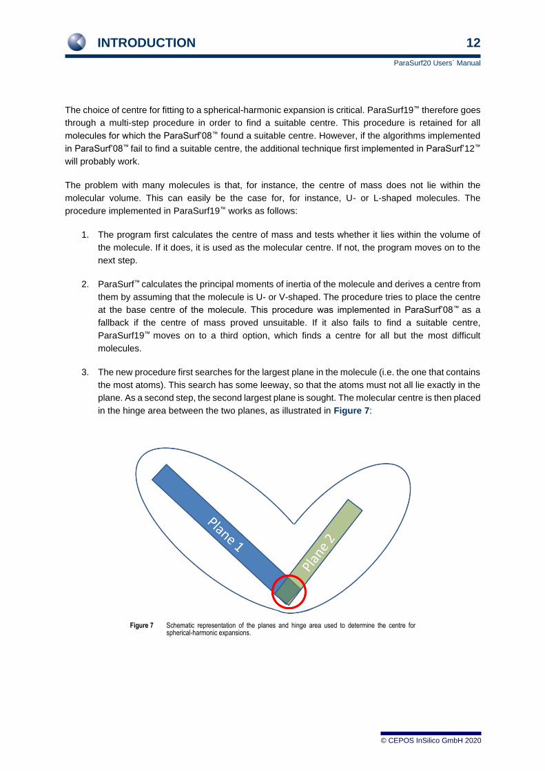
3. The new procedure first searches for the largest plane in the molecule (i.e. the one that contains
the most atoms). This search has some leeway, so that the atoms must not all lie exactly in the
plane. As a second step, the second largest plane is sought. The molecular centre is then placed
in the hinge area between the two planes, as illustrated in Figure 7:
Figure 7 Schematic representation of the planes and hinge area used to determine the centre for spherical-harmonic expansions.
INTRODUCTION 13
ParaSurf20 Users´ Manual
© CEPOS InSilico GmbH 2020
1.8 Local properties
The local properties calculated by ParaSurf™ are those related to intermolecular interactions. Local
properties, sometimes inaccurately called fields in QSAR work, are properties that vary in space around
the molecule and therefore have a distribution of values at the molecular surface. The best known and
most important local property in this context is the molecular electrostatic potential, which governs
Coulomb interactions, but the MEP only describes a part of the intermolecular interaction energy, so
that further local properties are needed.
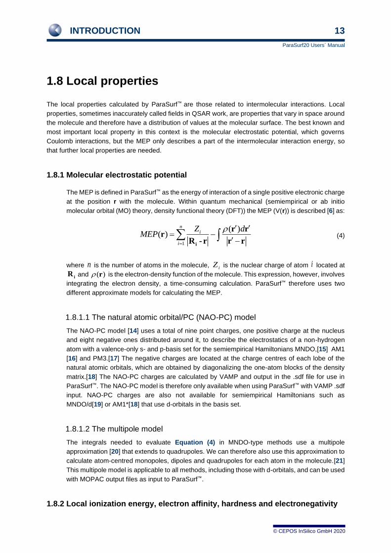
1.8.1 Molecular electrostatic potential
The MEP is defined in ParaSurf™ as the energy of interaction of a single positive electronic charge
at the position r with the molecule. Within quantum mechanical (semiempirical or ab initio
molecular orbital (MO) theory, density functional theory (DFT)) the MEP (V(r)) is described [6] as:
(4)
where is the number of atoms in the molecule, is the nuclear charge of atom located at
and is the electron-density function of the molecule. This expression, however, involves
integrating the electron density, a time-consuming calculation. ParaSurf™ therefore uses two
different approximate models for calculating the MEP.
1.8.1.1 The natural atomic orbital/PC (NAO-PC) model
The NAO-PC model [14] uses a total of nine point charges, one positive charge at the nucleus
and eight negative ones distributed around it, to describe the electrostatics of a non-hydrogen
atom with a valence-only s- and p-basis set for the semiempirical Hamiltonians MNDO,[15] AM1
[16] and PM3.[17] The negative charges are located at the charge centres of each lobe of the
natural atomic orbitals, which are obtained by diagonalizing the one-atom blocks of the density
matrix.[18] The NAO-PC charges are calculated by VAMP and output in the .sdf file for use in
ParaSurf™. The NAO-PC model is therefore only available when using ParaSurf™ with VAMP .sdf
input. NAO-PC charges are also not available for semiempirical Hamiltonians such as
MNDO/d[19] or AM1*[18] that use d-orbitals in the basis set.
1.8.1.2 The multipole model
The integrals needed to evaluate Equation (4) in MNDO-type methods use a multipole
approximation [20] that extends to quadrupoles. We can therefore also use this approximation to
calculate atom-centred monopoles, dipoles and quadrupoles for each atom in the molecule.[21]
This multipole model is applicable to all methods, including those with d-orbitals, and can be used
with MOPAC output files as input to ParaSurf™.
1.8.2 Local ionization energy, electron affinity, hardness and electronegativity
1
( )( )
ni
i
Z dMEP
=
= −
−
i
r rr
R -r r r
n iZ i
iR ( ) r

INTRODUCTION 14
ParaSurf20 Users´ Manual
© CEPOS InSilico GmbH 2020
The local ionization energy is defined [7] as a density-weighted Koopmans’ ionization
potential at a point near the molecule:
(5)
where is the number of the highest occupied MO, is the electron density at point
due to MO and is its Eigenvalue. The local ionization energy describes the tendency of
the molecule to interact with electron acceptors (Lewis acids) in a given region in space.[7-8]
The definition of the local electron affinity is a simple extension of Equation (5) to the virtual
MOs:[8]
(6)
The local electron affinity is the equivalent of the local ionization energy for interactions with
electron donors (Lewis bases).[8] An intensity-filtering technique [20b] was introduced in
ParaSurf’10™ to allow the local electron affinity to be calculated for Hamiltonians such as AM1*
and MNDO/d that use polarisation d-functions.
Equation (6) requires that the occupied and virtual orbitals be approximately equivalent to each
other. This is not the case for semiempirical Hamiltonians (such as AM1*) that include d-orbitals
as polarisation functions or for extensive basis sets in Hartree-Fock ab initio or in Density-
Functional theory (DFT) calculations. A new technique has therefore been defined [11] to exclude
pure polarisation functions from the summation in Equation (6). This technique is now default in
ParaSurf19™ and gives reliable results. For continuity, a new command-line option (EAL09) has
been introduced to request that the calculation of the local electron affinity be performed exactly
as in ParaSurf’09™ and earlier versions.
Two further, less fundamental local properties have been defined.[8] These are the local
hardness, :
(7)
and the local electronegativity, :
(8)
( )LIE r
r
1
1
( )
( )
( )
HOMO
i i
iL HOMO
i
i
IE
=
=
−
=
r
r
r
HOMO ( )i r
r ii
( )
( )
( )
norbs
i i
i LUMOL norbs
i
i LUMO
EA
=
=
−
=
r
r
r
L
( )2
L L
L
IE EA
−=
L
( )2
L L
L
IE EA
+=
INTRODUCTION 15
ParaSurf20 Users´ Manual
© CEPOS InSilico GmbH 2020
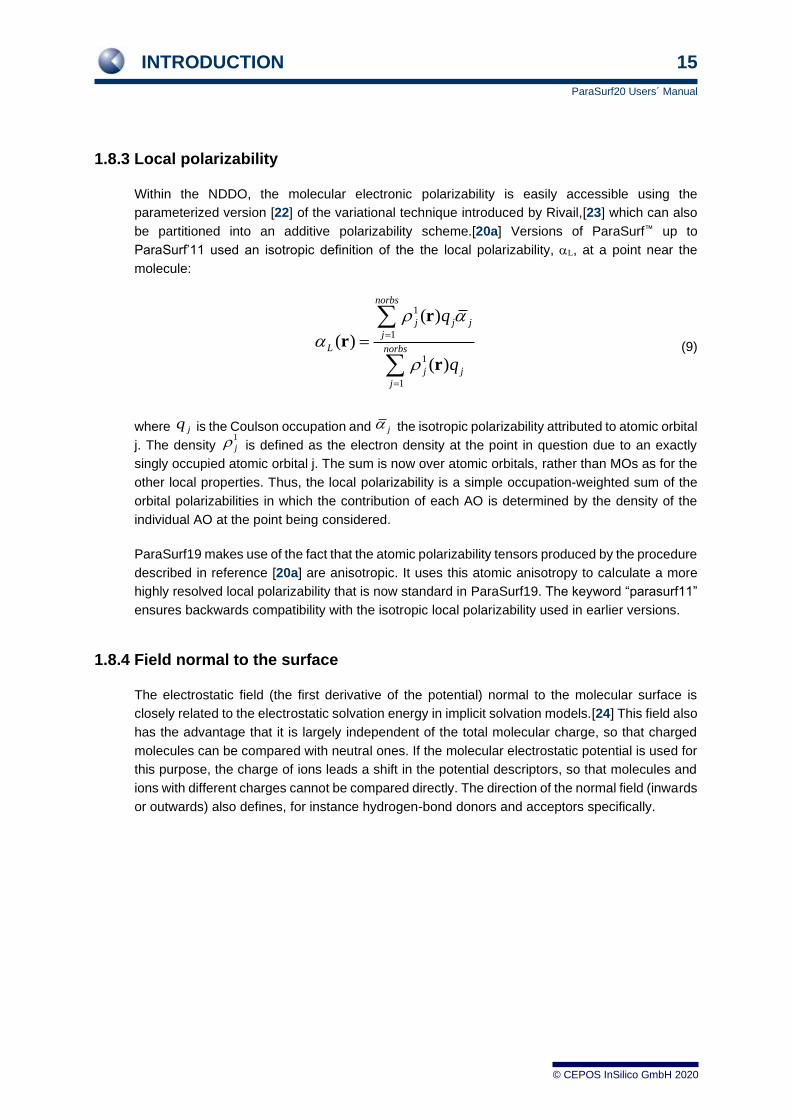
1.8.3 Local polarizability
Within the NDDO, the molecular electronic polarizability is easily accessible using the
parameterized version [22] of the variational technique introduced by Rivail,[23] which can also
be partitioned into an additive polarizability scheme.[20a] Versions of ParaSurf™ up to
ParaSurf’11 used an isotropic definition of the the local polarizability, L, at a point near the
molecule:
(9)
where is the Coulson occupation and the isotropic polarizability attributed to atomic orbital
j. The density is defined as the electron density at the point in question due to an exactly
singly occupied atomic orbital j. The sum is now over atomic orbitals, rather than MOs as for the
other local properties. Thus, the local polarizability is a simple occupation-weighted sum of the
orbital polarizabilities in which the contribution of each AO is determined by the density of the
individual AO at the point being considered.
ParaSurf19 makes use of the fact that the atomic polarizability tensors produced by the procedure
described in reference [20a] are anisotropic. It uses this atomic anisotropy to calculate a more
highly resolved local polarizability that is now standard in ParaSurf19. The keyword “parasurf11”
ensures backwards compatibility with the isotropic local polarizability used in earlier versions.
1.8.4 Field normal to the surface
The electrostatic field (the first derivative of the potential) normal to the molecular surface is
closely related to the electrostatic solvation energy in implicit solvation models.[24] This field also
has the advantage that it is largely independent of the total molecular charge, so that charged
molecules can be compared with neutral ones. If the molecular electrostatic potential is used for
this purpose, the charge of ions leads a shift in the potential descriptors, so that molecules and
ions with different charges cannot be compared directly. The direction of the normal field (inwards
or outwards) also defines, for instance hydrogen-bond donors and acceptors specifically.
1
1
1
1
( )
( )
( )
norbs
j j j
j
L norbs
j j
j
q
q
=
=
=
r
r
r
jq j1
j
INTRODUCTION 16
ParaSurf20 Users´ Manual
© CEPOS InSilico GmbH 2020
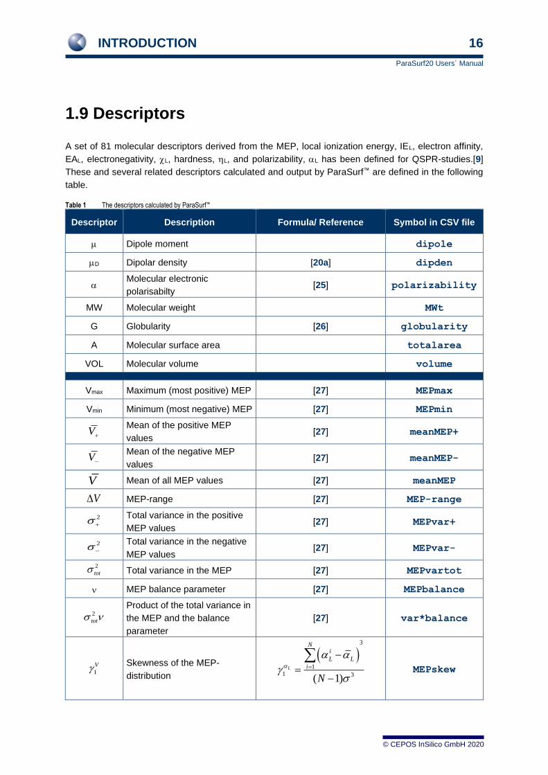
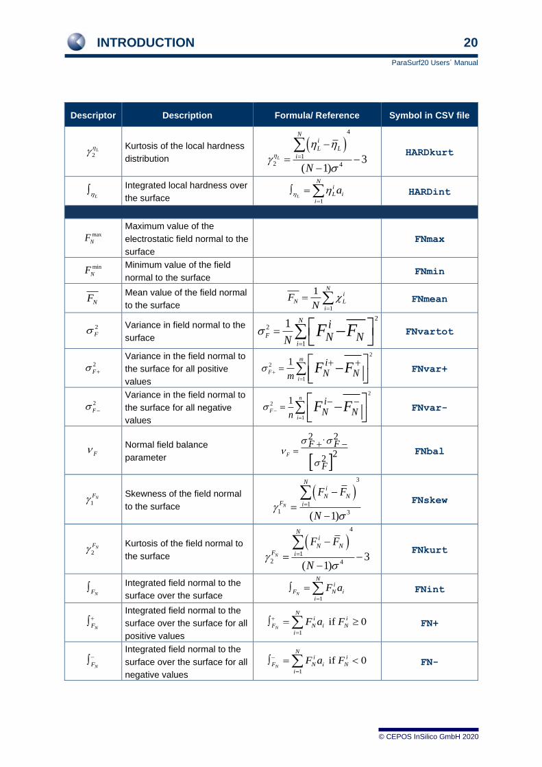
1.9 Descriptors
A set of 81 molecular descriptors derived from the MEP, local ionization energy, IEL, electron affinity,
EAL, electronegativity, L, hardness, L, and polarizability, L has been defined for QSPR-studies.[9]
These and several related descriptors calculated and output by ParaSurf™ are defined in the following
table.
Table 1 The descriptors calculated by ParaSurf™
Descriptor Description Formula/ Reference Symbol in CSV file
Dipole moment dipole
D Dipolar density [20a] dipden
Molecular electronic
polarisabilty [25] polarizability
MW Molecular weight MWt
G Globularity [26] globularity
A Molecular surface area totalarea
VOL Molecular volume volume
Vmax Maximum (most positive) MEP [27] MEPmax
Vmin Minimum (most negative) MEP [27] MEPmin
Mean of the positive MEP
values [27] meanMEP+
Mean of the negative MEP
values [27] meanMEP-
Mean of all MEP values [27] meanMEP
MEP-range [27] MEP-range
Total variance in the positive
MEP values [27] MEPvar+
Total variance in the negative
MEP values [27] MEPvar-
Total variance in the MEP [27] MEPvartot
MEP balance parameter [27] MEPbalance
Product of the total variance in
the MEP and the balance
parameter
[27] var*balance
Skewness of the MEP-
distribution
MEPskew
V+
V−
V
V
2 +
2 −
2
tot
2
tot
1
V( )
3
11 3( 1)
L
Ni
L L
i
N
=
−
=−

INTRODUCTION 17
ParaSurf20 Users´ Manual
© CEPOS InSilico GmbH 2020
Descriptor Description Formula/ Reference Symbol in CSV file
Kurtosis of the MEP-
distribution
MEPkurt
Integrated MEP over the
surface
MEPint
Maximum value of the local
ionization energy IELmax
Minimum value of the local
ionization energy IELmin
Mean value of the local
ionization energy IELbar
Range of the local ionization
energy IELrange
Variance in the local ionization
energy IELvar
Skewness of the local
ionization energy distribution IELskew
Kurtosis of the local ionization
energy distribution IELkurt
Integrated local ionization
energy over the surface IELint
Maximum of the local electron
affinity EALmax
Minimum of the local electron
affinity EALmin
Mean of the positive values of
the local electron affinity EALbar+
Mean of the negative values of
the local electron affinity EALbar-
Mean value of the local
electron affinity EALbar
Range of the local electron
affinity EALrange
2
V
V
max
LIE
min
LIE
LIE1
1 Ni
L L
i
IE IEN =
=
LIE max min
L L LIE IE IE = −
2
IE2
2
1
1 N
IE
i
iL LN
IE IE=
= −
1LIE
( )3
11 3( 1)
L
Ni
L LIE i
IE IE
N
=
−
=−
2LIE
( )4
12 4
3( 1)
L
Ni
L LIE i
IE IE
N
=
−
= −−
LIE1
L
Ni
IE L i
i
IE a=
=
max
LEA
min
LEA
LEA +
1
1 Ni
L L
i
EA EAN
+
+ ++=
=
LEA −
1
1 Ni
L L
i
EA EAN
−
− −−=
=
LEA1
1 Ni
L L
i
EA EAN =
=
LEA max min
L L LEA EA EA = −
( )4
12 4
3( 1)
N
iV i
V V
N
=
−
= −−
1
N
V i i
i
V a=
=

INTRODUCTION 18
ParaSurf20 Users´ Manual
© CEPOS InSilico GmbH 2020
Descriptor Description Formula/ Reference Symbol in CSV file
Variance in the local electron
affinity for all positive values
EALvar+
Variance in the local electron
affinity for all negative values
EALvar-
Sum of the positive and
negative variances in the local
electron affinity
EALvartot
Local electron affinity balance
parameter
EALbalance
Fraction of the surface area
with positive local electron
affinity
,
A = total surface area
EALfraction+
Surface area with positive
local electron affinity EALarea+
Skewness of the local electron
affinity distribution
EALskew
Kurtosis of the local electron
affinity distribution
EALkurt
Integrated local electron
affinity over the surface EALint
Maximum value of the local
polarizability POLmax
Minimum value of the local
polarizability POLmin
Mean value of the local
polarizability POLbar
Range of the local
polarizability POLrange
Variance in the local
polarizability POLvar
Skewness of the local
polarizability distribution POLskew
2
EA +
2
2
1
1 m
EA
iim
EA EA +
=
+ += −
2
EA −
2
2
1
1 n
EA
iin
EA EA −
=
− −= −
2
EAtot 2 2 2
EAtot EA EA + −= +
EA
2 2
22
EA
EA EA
EA
+ −
=
EA +EA
EA+
+ =
EA
+
1LEA
( )3
11 3( 1)
L
Ni
L LEA i
EA EA
N
=
−
=−
2LEA
( )4
12 4
3( 1)
L
Ni
L LEA i
EA EA
N
=
−
= −−
LEA1
L
Ni
IE L i
i
EA a=
=
max
L
min
L
L1
1 Ni
L L
iN
=
=
Lmax min
L L L = −
2
2
2
1
1 N
i
iL LN
=
= −
1L
( )3
11 3( 1)
L
Ni
L L
i
N
=
−
=−

INTRODUCTION 19
ParaSurf20 Users´ Manual
© CEPOS InSilico GmbH 2020
Descriptor Description Formula/ Reference Symbol in CSV file
Kurtosis of the local
polarizability distribution
POLkurt
Integrated local polarizability
over the surface POLint
Maximum value of the local
electronegativity ENEGmax
Minimum value of the local
electronegativity ENEGmin
Mean value of the local
electronegativity ENEGbar
Range of the local electron
electronegativity ENEGrange
Variance in the local
electronegativity ENEGvar
Skewness of the local
electronegativity distribution ENEGskew
Kurtosis of the local
electronegativity distribution ENEGkurt
Integrated local
electronegativity over the
surface
ENEGint
Maximum value of the local
hardness HARDmax
Minimum value of the local
hardness HARDmin
Mean value of the local
hardness HARDbar
Range of the local electron
hardness HARDrange
Variance in the local hardness
HARDvar
Skewness of the local
hardness distribution
HARDskew
2L
( )4
12 4
3( 1)
L
Ni
L L
i
N
=
−
= −−
L
1L
Ni
L i
i
a =
=
max
L
min
L
L1
1 Ni
L L
iN
=
=
Lmax min
L L L = −
2
2
2
1
1 N
i
iL LN
=
= −
1L
( )3
11 3( 1)
L
Ni
L L
i
N
=
−
=−
2L
( )4
12 4
3( 1)
L
Ni
L L
i
N
=
−
= −−
L
1L
Ni
L i
i
a =
=
max
L
min
L
L1
1 Ni
L L
iN
=
=
Lmax min
L L L = −
2
2
2
1
1 N
i
iL LN
=
= −
1L
( )3
11 3( 1)
L
Ni
L L
i
N
=
−
=−
INTRODUCTION 20
ParaSurf20 Users´ Manual
© CEPOS InSilico GmbH 2020
Descriptor Description Formula/ Reference Symbol in CSV file
Kurtosis of the local hardness
distribution
HARDkurt
Integrated local hardness over
the surface HARDint
Maximum value of the
electrostatic field normal to the
surface
FNmax
Minimum value of the field
normal to the surface FNmin
Mean value of the field normal
to the surface FNmean
Variance in field normal to the
surface FNvartot
Variance in the field normal to
the surface for all positive
values
FNvar+
Variance in the field normal to
the surface for all negative
values
FNvar-
Normal field balance
parameter FNbal
Skewness of the field normal
to the surface FNskew
Kurtosis of the field normal to
the surface FNkurt
Integrated field normal to the
surface over the surface FNint
Integrated field normal to the
surface over the surface for all
positive values
FN+
Integrated field normal to the
surface over the surface for all
negative values
FN-
2L
( )4
12 4
3( 1)
L
Ni
L L
i
N
=
−
= −−
L
1L
Ni
L i
i
a =
=
max
NF
min
NF
NF1
1 Ni
N L
i
FN
=
=
2
F
2
2
1
1 N
F
i
iN NN
F F=
= −
2
F +
2
2
1
1 m
F
i
iN Nm
F F +
=
+ += −
2
F −
2
2
1
1 n
F
i
iN Nn
F F −
=
− −= −
F
2 2
22
F
F F
F
+ −
=
1NF
( )3
11 3( 1)
N
Ni
N NF i
F F
N
=
−
=−
2NF
( )4
12 4
3( 1)
N
Ni
N NF i
F F
N
=
−
= −−
NF1
N
Ni
F N i
i
F a=
=
NF
+1
if 0N
Ni i
F N i N
i
F a F+
=
=
NF
−1
if 0N
Ni i
F N i N
i
F a F−
=
=

INTRODUCTION 21
ParaSurf20 Users´ Manual
© CEPOS InSilico GmbH 2020
Descriptor Description Formula/ Reference Symbol in CSV file
Integrated absolute field
normal to the surface over the
surface
FNabs
Additionally if the Shannon Entropy is calculated
Maximum value of the internal
Shannon Entropy SHANImax
Minimum value of the internal
Shannon Entropy SHANImin
Mean value of the internal
Shannon Entropy SHANIbar
Variance in the internal
Shannon Entropy
SHANIvar
Integrated internal Shannon
Entropy over the surface SHANItot
And if the external Shannon Entropy is available
Maximum value of the external
Shannon Entropy SHANEmax
Minimum value of the external
Shannon Entropy SHANEmin
Mean value of the external
Shannon Entropy SHANEbar
Variance in the external
Shannon Entropy
SHANEvar
Integrated internal Shannon
Entropy over the surface SHANEtot
NF
1N
Ni
F N i
i
F a=
=
max
inH
min
inH
inH1
1 Ni
in in
i
H HN =
=
2
inH
2
2
1
1in
N
H
i
iin inN
H H=
= −
inH1
in
Ni
H in i
i
H a=
=
max
exH
min
exH
exH1
1 Ni
ex ex
i
H HN =
=
2
exH
2
2
1
1ex
N
H
i
iex exN
H H=
= −
exH1
ex
Ni
H ex i
i
H a=
=

INTRODUCTION 22
ParaSurf20 Users´ Manual
© CEPOS InSilico GmbH 2020
1.10 Surface-integral models (polynomial version)
The polynomial surface-integral models that can be calculated by ParaSurf™ are defined [10] using the
expression
(10)
where is the target property, usually a free energy, is a polynomial function of the electrostatic
potential , the local ionization energy, , the local electron affinity, , the local polarizability,
and the local hardness, . is the area of the surface triangle .
The molecular property is printed to the output file and to the <filename>_p.sdf ParaSurf™
output SD-file. The individual values of the function are added to the list of local properties written
for each surface point to the .psf file if the surface details are output.
The surface-integral models themselves are not implemented directly in ParaSurf™, but are read in
general form from the SIM file, whose format is given in Section 3.11. Thus, the users’ own surface-
integral models can be added to ParaSurf™. Data for generating surface-integral models can be derived
simply from the .psf surface output for a normal ParaSurf™ run. Note that the program options given in
the SIM file must be the same for all the models included in the file and that they override conflicting
command-line options.
( )1
, , , ,ntri
i i i i i i
L L L L
i
P f V IE EA A =
=
P f
V LIE LEA
L LiA i
Pf
INTRODUCTION 23
ParaSurf20 Users´ Manual
© CEPOS InSilico GmbH 2020
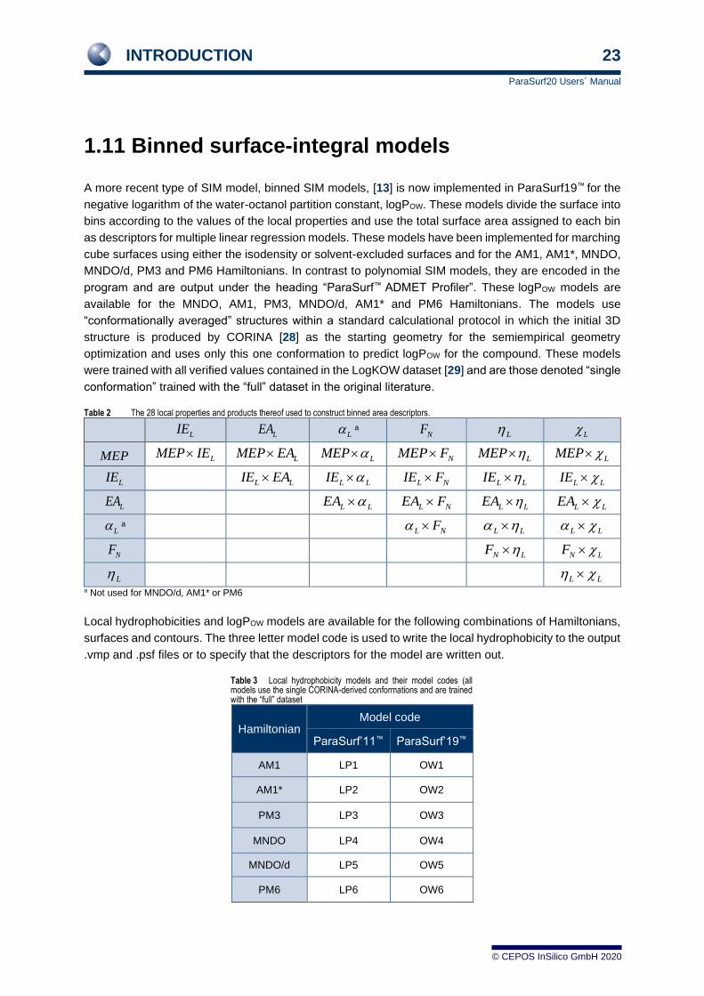
1.11 Binned surface-integral models
A more recent type of SIM model, binned SIM models, [13] is now implemented in ParaSurf19™ for the
negative logarithm of the water-octanol partition constant, logPOW. These models divide the surface into
bins according to the values of the local properties and use the total surface area assigned to each bin
as descriptors for multiple linear regression models. These models have been implemented for marching
cube surfaces using either the isodensity or solvent-excluded surfaces and for the AM1, AM1*, MNDO,
MNDO/d, PM3 and PM6 Hamiltonians. In contrast to polynomial SIM models, they are encoded in the
program and are output under the heading “ParaSurf™ ADMET Profiler”. These logPOW models are
available for the MNDO, AM1, PM3, MNDO/d, AM1* and PM6 Hamiltonians. The models use
“conformationally averaged” structures within a standard calculational protocol in which the initial 3D
structure is produced by CORINA [28] as the starting geometry for the semiempirical geometry
optimization and uses only this one conformation to predict logPOW for the compound. These models
were trained with all verified values contained in the LogKOW dataset [29] and are those denoted “single
conformation” trained with the “full” dataset in the original literature.
Table 2 The 28 local properties and products thereof used to construct binned area descriptors.
a
a
a Not used for MNDO/d, AM1* or PM6
Local hydrophobicities and logPOW models are available for the following combinations of Hamiltonians,
surfaces and contours. The three letter model code is used to write the local hydrophobicity to the output
.vmp and .psf files or to specify that the descriptors for the model are written out.
Table 3 Local hydrophobicity models and their model codes (all models use the single CORINA-derived conformations and are trained with the “full” dataset
Hamiltonian Model code
ParaSurf’11™ ParaSurf’19™
AM1 LP1 OW1
AM1* LP2 OW2
PM3 LP3 OW3
MNDO LP4 OW4
MNDO/d LP5 OW5
PM6 LP6 OW6
LIE LEA L NF L L
MEP LMEP IE LMEP EA LMEP NMEP F LMEP LMEP
LIE L LIE EA L LIE L NIE F L LIE L LIE
LEA L LEA L NEA F L LEA L LEA
L L NF L L L L
NF N LF N LF
L L L
INTRODUCTION 24
ParaSurf20 Users´ Manual
© CEPOS InSilico GmbH 2020
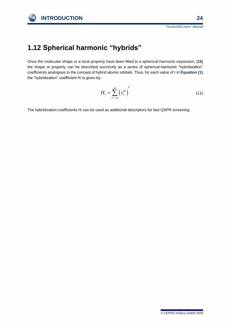
1.12 Spherical harmonic “hybrids”
Once the molecular shape or a local property have been fitted to a spherical-harmonic expansion, [16]
the shape or property can be described succinctly as a series of spherical-harmonic “hybridization”
coefficients analogous to the concept of hybrid atomic orbitals. Thus, for each value of l in Equation (1)
the “hybridization” coefficient Hl is given by:
(11)
The hybridization coefficients Hl can be used as additional descriptors for fast QSPR screening.
( )2m
m
l l
i m
H c=−
=
INTRODUCTION 25
ParaSurf20 Users´ Manual
© CEPOS InSilico GmbH 2020
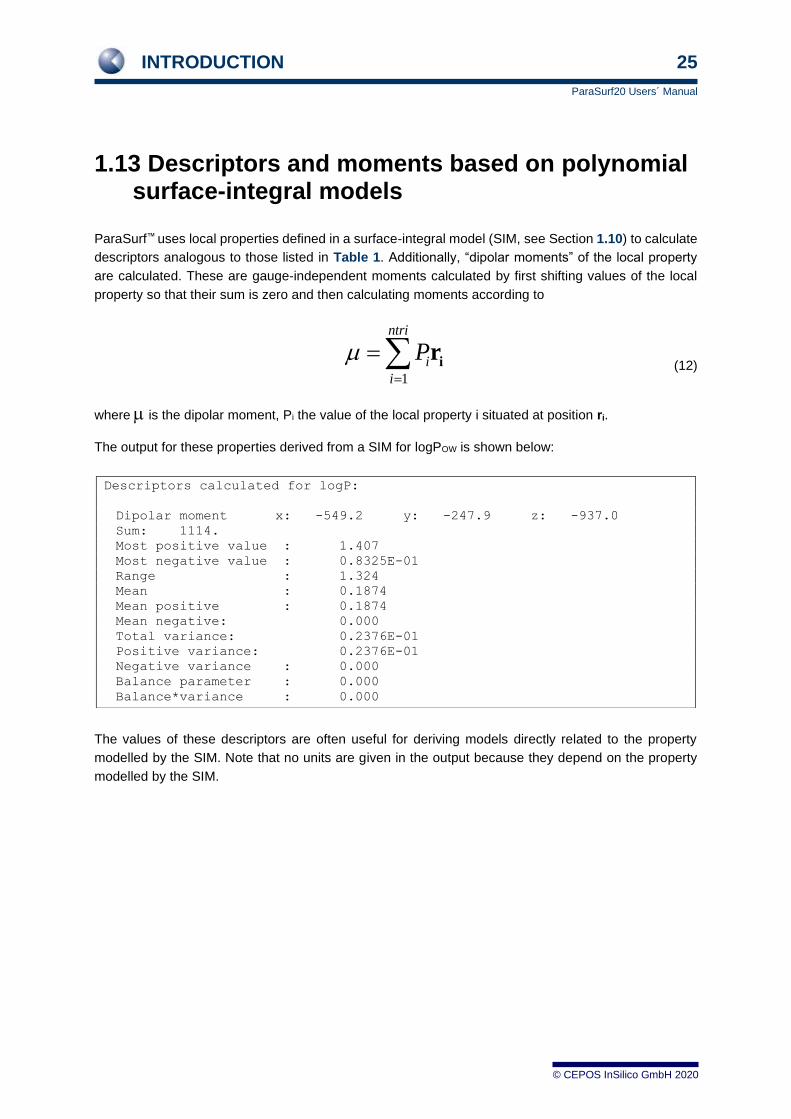
1.13 Descriptors and moments based on polynomial surface-integral models
ParaSurf™ uses local properties defined in a surface-integral model (SIM, see Section 1.10) to calculate
descriptors analogous to those listed in Table 1. Additionally, “dipolar moments” of the local property
are calculated. These are gauge-independent moments calculated by first shifting values of the local
property so that their sum is zero and then calculating moments according to
(12)
where is the dipolar moment, Pi the value of the local property i situated at position ri.
The output for these properties derived from a SIM for logPOW is shown below:
The values of these descriptors are often useful for deriving models directly related to the property
modelled by the SIM. Note that no units are given in the output because they depend on the property
modelled by the SIM.
1
ntri
i
i
P=
= ir
Descriptors calculated for logP:
Dipolar moment x: -549.2 y: -247.9 z: -937.0
Sum: 1114.
Most positive value : 1.407
Most negative value : 0.8325E-01
Range : 1.324
Mean : 0.1874
Mean positive : 0.1874
Mean negative: 0.000
Total variance: 0.2376E-01
Positive variance: 0.2376E-01
Negative variance : 0.000
Balance parameter : 0.000
Balance*variance : 0.000

INTRODUCTION 26
ParaSurf20 Users´ Manual
© CEPOS InSilico GmbH 2020
1.14 Shannon entropy
The information content at the surface of the molecule can be defined based on the distribution of the
four local properties over the surface using an approach analogous to that introduced by Shannon.[30]
Shannon defined the Shannon entropy, , which corresponds to the amount of information (in bits) as
(13)
where is the number of possible characters and is the probability that character will occur. Note
that, importantly, this definition of the amount of information is local (i.e. it only depends on the value of
the probability of character ).
For a continuous property, , Equation (13) becomes
(14)
If we now assume that the Shannon entropy at a point in space near a molecule is defined by the values
of the four continuous local properties described above, we obtain
(15)
where is the probability of finding the values and . However, we can simplify
this expression because the four properties are essentially independent of each other,[8-9] so that we
can write
(16)
Transferring this definition to a molecule for which a triangulated surface of triangles, where triangle
has area and average values of the four local properties , , and we obtain
(17)
where is the probability that the value of the property , where may be , , or
, will occur.
ParaSurf™ offers two alternatives as sources for the probabilities . The first, known as the
“external” Shannon entropy, is to use probabilities taken from an external dataset and defined in a
separate statistics file. The default “external” statistics file is called bins.txt and is read from the
H
( )2
1
logn
i i
i
H p p=
= −
n ip i
i
X
2( ) log ( )H p X p X dX
−
= −
( ) ( )2, , , log , , ,H p V I E V I E dVdIdEd = −
( ), , ,p V I E , ,V I E
( ) ( ) ( ) ( )
( ) ( ) ( ) ( )
2 2
2 2
log log
log log
H p V p V dV p I p I dI
p E p E dE p p d
= − −
− −
ki
iA iV iI iE i
2 2 2 2
1
( ) log ( ) ( ) log ( ) ( ) log ( ) ( ) log ( )k
i i i i i i i i i
i
H p V p V p I p I p E p E p p A =
= − + + +
( )ip X iX X X V I E
( )ip X

INTRODUCTION 27
ParaSurf20 Users´ Manual
© CEPOS InSilico GmbH 2020
ParaSurf™ root directory. The statistics defined in bins.txt were derived from AM1 calculations of
all the bound ligands defined in the PDBbind database [31] in their correct protonation states and at
geometries obtained by optimizing with AM1 starting from the bound conformation.[27]
Alternatively, the user can define a custom “external” statistics file using the ParaSurf™ module binner
(available free of charge for ParaSurf™ users). The “external” Shannon entropy is useful for relating a
series of molecules to each other, but is sensitive, for instance, to the total charge of the molecule.
The “internal” Shannon entropy is calculated using probabilities determined from the surface properties
of the molecule itself, and therefore corresponds more closely to Shannon’s classical definition than the
“external” Shannon entropy and the probabilities used are individual for each molecule. The “internal”
Shannon entropy can be considered to represent the information content of the molecule. The properties
of the two types of Shannon entropy will be described in a forthcoming paper.
INTRODUCTION 28
ParaSurf20 Users´ Manual
© CEPOS InSilico GmbH 2020
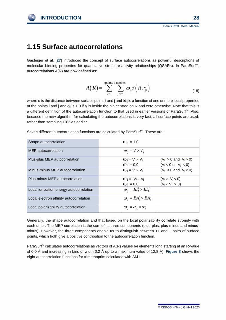
1.15 Surface autocorrelations
Gasteiger et al. [27] introduced the concept of surface autocorrelations as powerful descriptions of
molecular binding properties for quantitative structure-activity relationships (QSARs). In ParaSurf™,
autocorrelations A(R) are now defined as:
(18)
where rij is the distance between surface points i and j and ij is a function of one or more local properties
at the points i and j and ij is 1.0 if rij is inside the bin centred on R and zero otherwise. Note that this is
a different definition of the autocorrelation function to that used in earlier versions of ParaSurf™. Also,
because the new algorithm for calculating the autocorrelations is very fast, all surface points are used,
rather than sampling 10% as earlier.
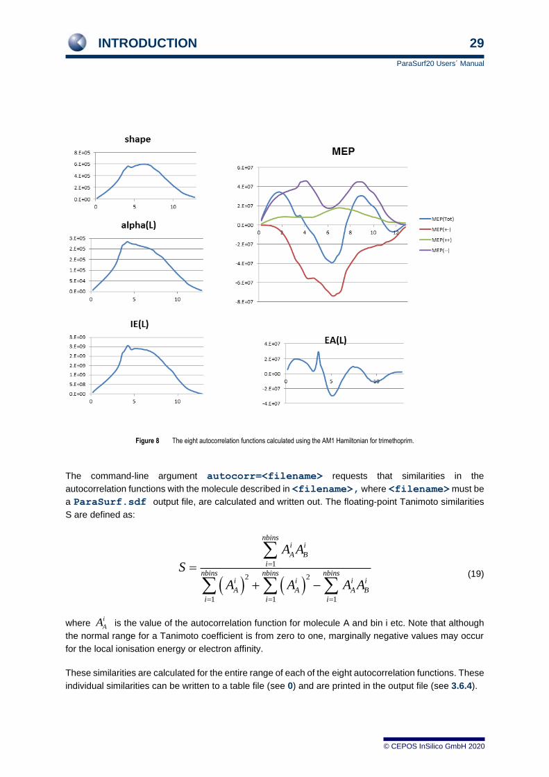
Seven different autocorrelation functions are calculated by ParaSurf™. These are:
Shape autocorrelation ij = 1.0
MEP autocorrelation ij i jV V =
Plus-plus MEP autocorrelation ij = Vi Vj
ij = 0.0
(Vi > 0 and Vj > 0)
(Vi < 0 or Vj < 0)
Minus-minus MEP autocorrelation ij = Vi Vj (Vi < 0 and Vj < 0)
Plus-minus MEP autocorrelation ij = -Vi Vj
ij = 0.0
(Vi Vj < 0)
(Vi Vj > 0)
Local ionization energy autocorrelation i j
ij L LIE IE =
Local electron affinity autocorrelation i j
ij L LEA EA =
Local polarizability autocorrelation i j
ij L L =
Generally, the shape autocorrelation and that based on the local polarizability correlate strongly with
each other. The MEP correlation is the sum of its three components (plus-plus, plus-minus and minus-
minus). However, the three components enable us to distinguish between ++ and – pairs of surface
points, which both give a positive contribution to the autocorrelation function.
ParaSurf™ calculates autocorrelations as vectors of A(R) values 64 elements long starting at an R-value
of 0.0 Å and increasing in bins of width 0.2 Å up to a maximum value of 12.8 Å). Figure 8 shows the
eight autocorrelation functions for trimethoprim calculated with AM1.
( ) ( )npoints-1 npoints
ij
1 j=i+1
, ij
i
A R R r =
=
INTRODUCTION 29
ParaSurf20 Users´ Manual
© CEPOS InSilico GmbH 2020
Figure 8 The eight autocorrelation functions calculated using the AM1 Hamiltonian for trimethoprim.
The command-line argument autocorr=<filename> requests that similarities in the
autocorrelation functions with the molecule described in <filename>, where <filename> must be
a ParaSurf.sdf output file, are calculated and written out. The floating-point Tanimoto similarities
S are defined as:
( ) ( )
1
2 2
1 1 1
nbinsi i
A B
i
nbins nbins nbinsi i i i
A A A B
i i i
A A
S
A A A A
=
= = =
=
+ −
(19)
where i
AA is the value of the autocorrelation function for molecule A and bin i etc. Note that although
the normal range for a Tanimoto coefficient is from zero to one, marginally negative values may occur
for the local ionisation energy or electron affinity.
These similarities are calculated for the entire range of each of the eight autocorrelation functions. These
individual similarities can be written to a table file (see 0) and are printed in the output file (see 3.6.4).
INTRODUCTION 30
ParaSurf20 Users´ Manual
© CEPOS InSilico GmbH 2020
1.16 Standard rotationally invariant fingerprints (RIFs)
Mavridis et al. [32] introduced standard rotationally invariant fingerprints (RIFs) based on the spherical-
harmonic hybridization coefficients defined above. These fingerprints provide a detailed description of
the molecular shape, electrostatics, donor/acceptor properties and polarizability as a standard series of
54 floating point numbers.
1.17 Maxima and minima of the local properties
Jakobi et al. [33] have described the calculation and use of the most significant maxima and minima of
the local properties on the surface of the molecule. These points were used in the ParaFrag procedure
to detect scaffold hops with high similarity and can be viewed as pharmacophore points.
1.18 Atom-centred descriptors
Hennemann et al. [34] have used atom-centred quantities calculated by ParaSurf™ as descriptors in
order to calculate the strengths of hydrogen bonds [34a] and for chemical reactivity models [34b]. These
descriptors (based on conventional solvent-accessible surface areas [35] using Bondi van der Waals
radii [36] and a default solvent radius of 1.4 Å), C-H bond orders for hydrogen atoms, the constitution of
the localized lone-pair orbitals on nitrogen atoms and the -charges of carbon atoms in conjugated -
systems. These descriptors are now output by ParaSurf19™.
1.19 Fragment analysis
ParaSurf19™ can divide the input molecule into fragments (which must be defined in the input SDF file)
and perform a full surface analysis for each fragment. This option and its output will be described in
detail below. ParaSurf19™ now outputs .psf and .sdf files for each fragment for use in CImatch19™ for
substructure similarity.

PROGRAM OPTIONS 31
ParaSurf20 Users´ Manual
© CEPOS InSilico GmbH 2020
2 PROGRAM OPTIONS
2.1 Command-line options
ParaSurf™ program options are given as command-line arguments. Arguments are separated by blanks,
so that no single argument may contain a blank character. Arguments may be written in any combination
of upper and lower case. The options are:
Table 4 ParaSurf™ command-line options
<name> Base name for the input file (must be the first
argument).<name> is not required if the first argument is –
version (see below).
The full file name can be given, in which case the name will be
used unchanged as input.
If an abbreviated file name
is used, the input file is
assumed to be
if a file with this name exists.
<name>_e.h5
Otherwise, the input file is
assumed to be
if a file with this name exists.
<name>_e.vwf
Otherwise an SDF file will
be used as input in the order
given.
<name>_v.sdf
<name>.sdf
If neither of these files are
found, the program will use
an .sdf file written by the
Cepos version of Mopac 6.
These files are called
<name>_m.sdf
The output files are
<name>_p.out
<name>_p.sdf
<name>.psf (optional)
<name>.asd (optional)
<name>_p.vmp (optional)
inlist= <filename> Alternatively, the first argument can give the name of a text file
containing a list of input files. The name of the output files will
be derived from the name of the list file. Any eligible input file
type can be given in the input list and mixtures of different file
types are accepted. The hierarchy of input file types defined
above applies.
surf= wrap
cube
Shrink-wrap surface (default)
Marching-cube surface

PROGRAM OPTIONS 32
ParaSurf20 Users´ Manual
© CEPOS InSilico GmbH 2020
contour= isoden
solvex
The surface is defined by the electron density
A solvent-excluded surface is used.
fit= sphh
isod
none
Spherical-harmonic fitting (default for surf=wrap)
Smooth to preset isodensity value (default for surf=cube)
No fitting
iso= n.nn Isodensity value set to n.nn e-Å-3
(default for shrink-wrap surface = 0.0005;
default for marching-cube surface = 0.007;
minimum possible value = 0.00001)
rsol= n.nn A solvent-probe radius of n.nn Å is used for calculating the
solvent-excluded or solvent-accessible surface (default=1.0,
allowed range is from 0.0 to 2.0 Å)
mesh= n.nn The mesh size used to triangulate the surface is set to n.nn
Å (default value = 0.2 Å, allowed range is from 0.1 to 1.0
Å)
estat= naopc
multi
newmp
Use NAO-PC electrostatics
Use multipole electrostatics (gives ParaSurf’11 electrostatics with the
“parasurf11” keyword, otherwise ParaSurf19)
Use ParaSurf’12 or 19 multipole electrostatics (default)
psf= on
off
Write .psf surface file
Do not write .psf surface file (default)
asd= on
off
Write anonymous SD (.asd) file
Do not write .asd file (default)
vmp= on
off
mep
iel
eal
pol
har
eng
anr
fnm
sha
<MOD>
Write .vmp file for debugging. Map the MEP onto the surface
Do not write .vmp file (default)
Write .vmp file for debugging. Map the MEP onto the surface
Write .vmp file for debugging. Map IEL onto the surface
Write .vmp file for debugging. Map EAL onto the surface
Write .vmp file for debugging. Map L onto the surface
Write .vmp file for debugging. Map L onto the surface
Write .vmp file for debugging. Map L onto the surface
Write .vmp file for debugging. Map the number of the atom
assigned to the surface element onto the surface
Write .vmp file for debugging. Map FN onto the surface
Write .vmp file for debugging. Map the Shannon entropy onto
the surface
Write .vmp file for debugging. Map the local property with the
three-character designator <MOD> defined in the SIM file onto
the surface

PROGRAM OPTIONS 33
ParaSurf20 Users´ Manual
© CEPOS InSilico GmbH 2020
vmpfrag= on
off
all
Equivalent to vmp=, but writes separate .vmp files for each
fragment with only its atoms and the MEP projected onto the
fragment surface. The files are named
<filename><fragmentname>.vmp, where
<fragmentname> is the name assigned to the fragment in
the input SDF file.
No fragment .vmp files will be written.
As for on, except that the atoms for the entire molecule are
written to the .vmp files with the surface for the fragment only.
grid= <filename>
auto
vdw
box
surf
Read the Cartesian coordinates at which to calculate a grid of
(log10(), MEP, IEL, EAL, L, L, L and their first derivatives in
x, y and z-directions). See Section 3.10.1
ParaSurf™ calculates an automatic grid that excludes areas
closer than 0.5 Å to the nuclei (see Section 3.10.2)
ParaSurf™ calculates an automatic grid that excludes areas
closer than the corresponding van der Waals radius to the
nuclei
ParaSurf™ calculates an automatic grid including all points
regardless of their proximity to nuclei
The properties of the surface points are written to the .psf file
lattice= n.nn Sets the lattice spacing for the grid=auto, vdw or box
option (see Section 3.10.2)
sim= <filename> One or more surface-integral models will be read from the file
<filename>.sim in the ParaSurf™ root directory.
<filename> can be upper or lower case or any mixture but
must be exactly three characters long.
center=
or
on The atomic and surface coordinates in the .psf output file
will be centred for calculations that use spherical-harmonic
fitting. Note that this means that the atomic coordinates in the
SDF-output file (which are the input coordinates) will be
different to those in the PSF-output file. This option is default.
centre= off The atomic and surface coordinates in the .psf output file
will not be centred and will correspond to the input coordinates
and those in the SDF-output file.
shannon =<filename> Requests that Shannon entropies (both internal and external)
be calculated. If no statistics file <filename> is given, the
default file (bins.txt in the ParaSurf™ Root directory) will
be used. If a statistics file is given that either does not exist,
contains errors or is derived from ParaSurf™ runs using
different options to the current one, only the internal Shannon
entropy is calculated.
autocorr =<filename> Requests that the surface autocorrelation functions be
calculated and written to the output .sdf file.
<filename> must be a ParaSurf™ output .sdf file that
contains the autocorrelation functions. In this case, similarities
between the two molecules will be calculated and printed (see
also aclist=).
PROGRAM OPTIONS 34
ParaSurf20 Users´ Manual
© CEPOS InSilico GmbH 2020
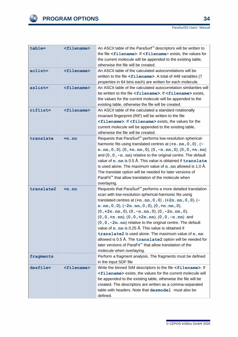
table= <filename> An ASCII table of the ParaSurf™ descriptors will be written to
the file <filename>. If <filename> exists, the values for
the current molecule will be appended to the existing table,
otherwise the file will be created.
aclist= <filename> An ASCII table of the calculated autocorrelations will be
written to the file <filename>. A total of 448 variables (7
properties in 64 bins each) are written for each molecule.
aslist= <filename> An ASCII table of the calculated autocorrelation similarities will
be written to the file <filename>. If <filename> exists,
the values for the current molecule will be appended to the
existing table, otherwise the file will be created.
riflist= <filename> An ASCII table of the calculated a standard rotationally
invariant fingerprint (RIF) will be written to the file
<filename>. If <filename> exists, the values for the
current molecule will be appended to the existing table,
otherwise the file will be created.
translate =n.nn Requests that ParaSurf™ performs low-resolution spherical-
harmonic fits using translated centres at (+n.nn,0,0) , (-
n.nn,0,0), (0,+n.nn,0), (0,-n.nn,0), (0,0,+n.nn)
and (0,0,-n.nn) relative to the original centre. The default
value of n.nn is 0.5 Å. This value is obtained if translate
is used alone. The maximum value of n.nn allowed is 1.0 Å.
The translate option will be needed for later versions of
ParaFit™ that allow translation of the molecule when
overlaying.
translate2 =n.nn Requests that ParaSurf™ performs a more detailed translation
scan with low-resolution spherical-harmonic fits using
translated centres at (+n.nn,0,0) , (+2n.nn,0,0), (-
n.nn,0,0), (-2n.nn,0,0), (0,+n.nn,0),
(0,+2n.nn,0), (0,-n.nn,0), (0,-2n.nn,0),
(0,0,+n.nn), (0,0,+2n.nn), (0,0,-n.nn) and
(0,0,-2n.nn) relative to the original centre. The default
value of n.nn is 0.25 Å. This value is obtained if
translate2 is used alone. The maximum value of n.nn
allowed is 0.5 Å. The translate2 option will be needed for
later versions of ParaFit™ that allow translation of the
molecule when overlaying.
fragments Perform a fragment analysis. The fragments must be defined
in the input SDF file
desfile= <filename> Write the binned SIM descriptors to the file <filename>. If
<filename> exists, the values for the current molecule will
be appended to the existing table, otherwise the file will be
created. The descriptors are written as a comma-separated
table with headers. Note that desmodel must also be
defined.

PROGRAM OPTIONS 35
ParaSurf20 Users´ Manual
© CEPOS InSilico GmbH 2020
desmodel= <code> The bin definitions for the model denoted by <code> will be
used to calculate the descriptors for the table of binned SIM
descriptors. The possible values of <code> and their
definitions are given in Table 2.
-version Must be the first argument. Requests that ParaSurf™ prints the
version number to the standard output channel and then stops
without performing a calculation.
eal09
Do not use the selection procedure for virtual orbitals [11]
when calculating the local electron affinity. This option
provides continuity with earlier versions of ParaSurf™
parasurf11
Backwards compatibility option: electron densities, local
properties and electrostatic potential and field are calculated
using the algorithms from ParaSurf’11
precise More precise output of the local properties in grid calculations
locpol= aniso
old
Use the local polarizability calculated from anisotropic atomic
polarizability tensors (default)
Use isotropic atomic polarizabilities to calculate the local
polarizability (implied by the “parasurf11” option)
no_derivatives
Do not calculate the first derivatives of the local properties
(default is to calculate the derivatives)
Examples:
parasurf test surf=wrap fit=sphh iso=0.03 psf=on estat=naopc
Use the input file test_e.h5, test_e.vwf, test_m.sdf, test.sdf or test_m.sdf to
calculate a shrink-wrap surface with an isodensity value of 0.03 e-Å-3, perform a spherical-harmonic fit,
use NAO-PC electrostatics and write the spherical-harmonic coefficients to test_P.sdf and the
entire surface to test_P.psf.
parasurf test_e.h5 surf=cube fit=none
Use the file test_e.h5 as input to perform a marching-cube surface determination without fitting and
to calculate the descriptor set.
PROGRAM OPTIONS 36
ParaSurf20 Users´ Manual
© CEPOS InSilico GmbH 2020
2.2 Options defined in the input SDF-file
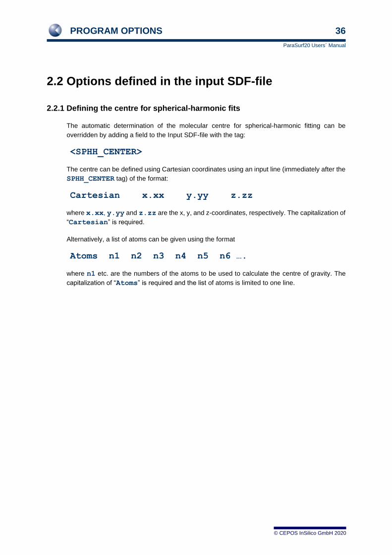
2.2.1 Defining the centre for spherical-harmonic fits
The automatic determination of the molecular centre for spherical-harmonic fitting can be
overridden by adding a field to the Input SDF-file with the tag:
<SPHH_CENTER>
The centre can be defined using Cartesian coordinates using an input line (immediately after the
SPHH_CENTER tag) of the format:
Cartesian x.xx y.yy z.zz
where x.xx, y.yy and z.zz are the x, y, and z-coordinates, respectively. The capitalization of
“Cartesian” is required.
Alternatively, a list of atoms can be given using the format
Atoms n1 n2 n3 n4 n5 n6 ….
where n1 etc. are the numbers of the atoms to be used to calculate the centre of gravity. The
capitalization of “Atoms” is required and the list of atoms is limited to one line.
PROGRAM OPTIONS 37
ParaSurf20 Users´ Manual
© CEPOS InSilico GmbH 2020
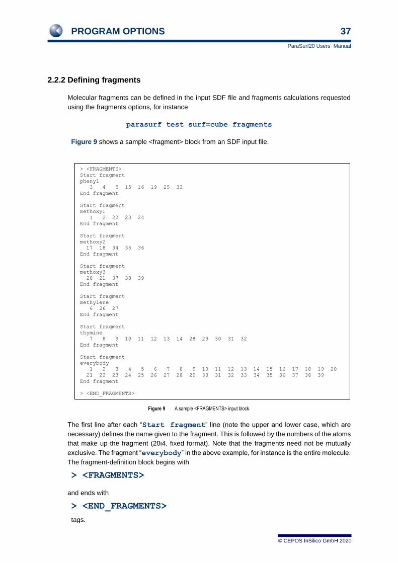
2.2.2 Defining fragments
Molecular fragments can be defined in the input SDF file and fragments calculations requested
using the fragments options, for instance
parasurf test surf=cube fragments
Figure 9 shows a sample <fragment> block from an SDF input file.
Figure 9 A sample <FRAGMENTS> input block.
The first line after each “Start fragment” line (note the upper and lower case, which are
necessary) defines the name given to the fragment. This is followed by the numbers of the atoms
that make up the fragment (20i4, fixed format). Note that the fragments need not be mutually
exclusive. The fragment “everybody” in the above example, for instance is the entire molecule.
The fragment-definition block begins with
> <FRAGMENTS>
and ends with
> <END_FRAGMENTS>
tags.
> <FRAGMENTS>
Start fragment
phenyl
3 4 5 15 16 19 25 33
End fragment
Start fragment
methoxy1
1 2 22 23 24
End fragment
Start fragment
methoxy2
17 18 34 35 36
End fragment
Start fragment
methoxy3
20 21 37 38 39
End fragment
Start fragment
methylene
6 26 27
End fragment
Start fragment
thymine
7 8 9 10 11 12 13 14 28 29 30 31 32
End fragment
Start fragment
everybody
1 2 3 4 5 6 7 8 9 10 11 12 13 14 15 16 17 18 19 20
21 22 23 24 25 26 27 28 29 30 31 32 33 34 35 36 37 38 39
End fragment
> <END_FRAGMENTS>
PROGRAM OPTIONS 38
ParaSurf20 Users´ Manual
© CEPOS InSilico GmbH 2020
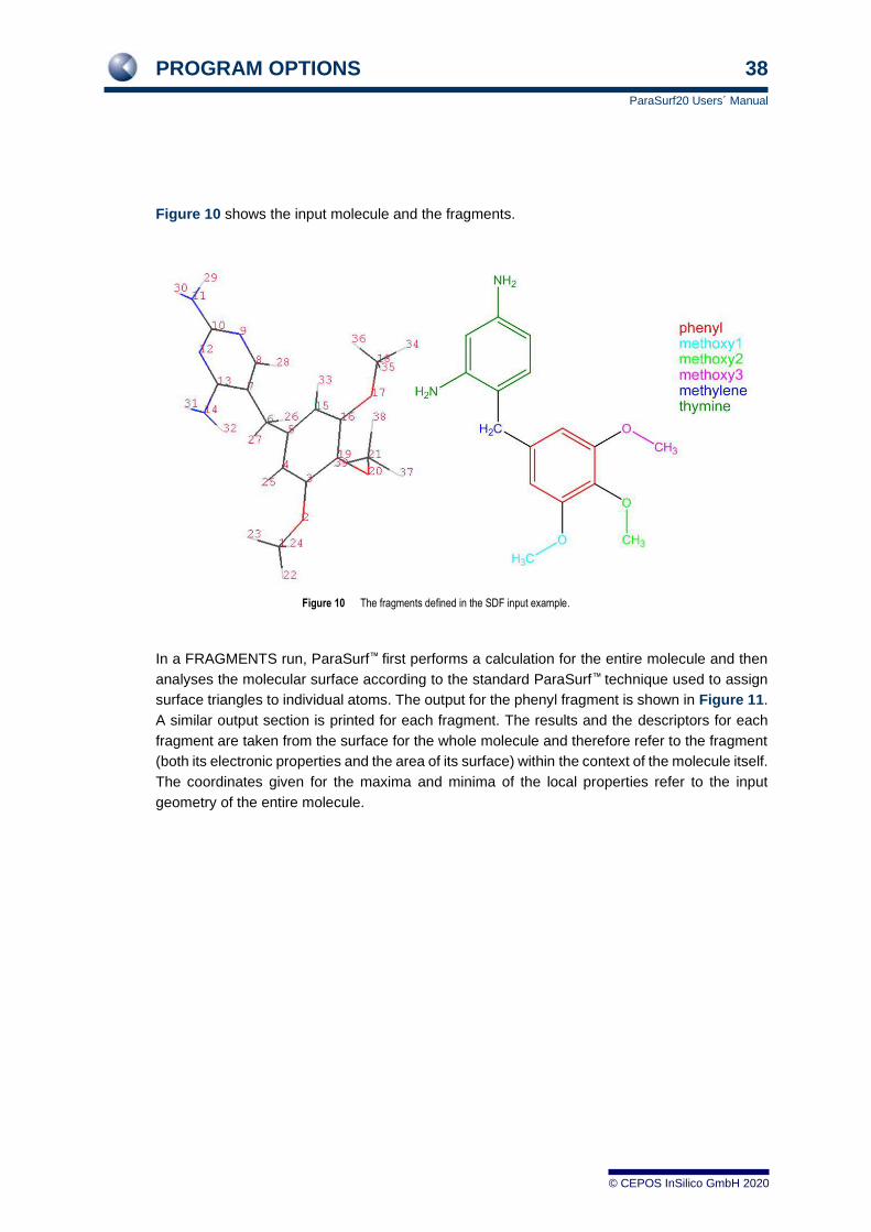
Figure 10 shows the input molecule and the fragments.
Figure 10 The fragments defined in the SDF input example.
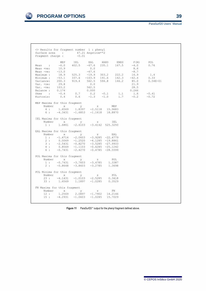
In a FRAGMENTS run, ParaSurf™ first performs a calculation for the entire molecule and then
analyses the molecular surface according to the standard ParaSurf™ technique used to assign
surface triangles to individual atoms. The output for the phenyl fragment is shown in Figure 11.
A similar output section is printed for each fragment. The results and the descriptors for each
fragment are taken from the surface for the whole molecule and therefore refer to the fragment
(both its electronic properties and the area of its surface) within the context of the molecule itself.
The coordinates given for the maxima and minima of the local properties refer to the input
geometry of the entire molecule.
PROGRAM OPTIONS 39
ParaSurf20 Users´ Manual
© CEPOS InSilico GmbH 2020
Figure 11 ParaSurf20™ output for the phenyl fragment defined above.
<> Results for fragment number 1 : phenyl
Surface area : 47.21 Angstrom**2
Fragment charge : -0.01
MEP IEL EAL HARD ENEG F(N) POL
Mean : -6.0 402.5 -67.6 235.1 167.5 -4.0 0.76
Mean +ve: 10.9 0.0 8.6
Mean -ve: -13.0 -67.6 -8.7
Maximum : 18.9 525.3 -19.9 303.2 222.2 16.9 1.4
Minimum : -53.1 337.6 -103.9 191.6 142.3 -42.4 0.33
Variance: 200.3 919.4 562.5 594.8 146.2 85.0 0.54E-01
Var. +ve: 29.8 0.0 21.9
Var. -ve: 103.2 562.5 28.5
Balance : 0.174 0.000 0.246
Skew : -0.4 0.7 0.2 -0.1 1.1 1.6 -0.41
Kurtosis: 0.4 0.6 -1.3 -1.0 1.7 -0.2 -0.72
MEP Maxima for this fragment
Number x y z MEP
4 : 1.6569 1.8397 -2.5118 15.9683
6 : -4.3431 -1.6853 -1.1618 18.8870
IEL Maxima for this fragment
Number x y z IEL
1 : 1.6861 -2.6103 -3.4142 525.3250
EAL Maxima for this fragment
Number x y z EAL
1 : -1.4714 -2.0603 -3.9285 -22.4779
2 : 0.0069 -1.2520 -4.1285 -19.8861
3 : -2.5431 -0.8270 -3.5285 -27.9933
4 : 0.8569 -1.1103 -0.6285 -25.1242
6 : -0.7431 -2.4270 -0.4785 -28.5599
POL Maxima for this fragment
Number x y z POL
1 : -0.7431 -3.7603 -3.4785 1.3387
2 : -0.8648 -3.8603 -3.2785 1.3698
POL Minima for this fragment
Number x y z POL
23 : -4.1431 -1.0103 -2.5285 0.3418
33 : 1.6569 1.1897 -1.0285 0.3529
FN Maxima for this fragment
Number x y z FN
12 : 1.2569 2.0897 -1.7902 14.2146
15 : -4.2931 -1.0603 -1.0285 15.7029
FN Minima for this fragment
Number x y z FN
4 : -2.4264 -0.6603 -3.5285 -15.7395
5 : -0.5931 0.5397 -3.7285 -15.8022
9 : -1.5431 -2.0103 -0.2285 -16.7298
10 : -0.0014 -0.0603 -0.2785 -18.9320
________________________________________________________________________________
PROGRAM OPTIONS 40
ParaSurf20 Users´ Manual
© CEPOS InSilico GmbH 2020
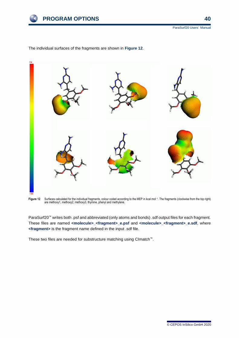
The individual surfaces of the fragments are shown in Figure 12.
Figure 12 Surfaces calculated for the individual fragments, colour coded according to the MEP in kcal mol−1. The fragments (clockwise from the top right) are methoxy1, methoxy2, methoxy3, thymine, phenyl and methylene.
ParaSurf20™ writes both .psf and abbreviated (only atoms and bonds) .sdf output files for each fragment.
These files are named <molecule>_<fragment>_e.psf and <molecule>_<fragment>_e.sdf, where
<fragment> is the fragment name defined in the input .sdf file.
These two files are needed for substructure matching using CImatch™.

INPUT AND OUTPUT FILES 41
ParaSurf20 Users´ Manual
© CEPOS InSilico GmbH 2020
3 INPUT AND OUTPUT FILES
ParaSurf™ uses the following files for input and output:
Table 5 ParaSurf™ input and output files
File Name Description
Input <filename>
<filename>_e.h5
(if available) or
<filename>.vwf
(if available) or
<filename>_v.sdf
or
<filename>.sdf
or
<filename>_m.sdf
The complete filename with extension.
EMPIRE™_e.h5 file
EMPIRE™.vwf file
VAMP.sdf file output.
VAMP must be run with the ALLVECT option to be able
to calculate all the properties. The VAMP version used
must be able to calculate AO-polarizabilities.
An input SDF file, typically produced by EMPIRE™ or
VAMP
If no VAMP.sdf file is found, ParaSurf™ defaults to a
CeposMopac 6.sdf file. It is strongly recommended to
use the EF option for geometry optimizations in Mopac.
alternatively
Inlist
The alternative input option is to define a file in which the
input files to be calculated are listed (one per row). All file
types can be used and mixed. The file-type rules given
above apply.
Hamiltonian <Hamiltonian>.par The EMPIRE parameters file (found in the EMPIRE etc directory). The environment variable EMPIRE_ROOT
must be set to point to this directory. The name <Hamiltonian> will be taken from the input SDF file.
Calculations using the hpCADD Hamiltonian must use an _e.h5 or .vwf file as input because atom types are not
defined in SDF files. In these cases, the <Hamiltonian>.par file is not required. The
parameters are read from the input file.
Output <filename>_p.out Always written.
SD-file <filename>_p.sdf Always written.
ASD-file <filename>.asd Anonymous SD-file. Requested by the option asd=on
PSF-file <filename>.psf ParaSurf™ surface file. Requested by the option psf=on
VMP-file <filename>_p.vmp Debug file.

INPUT AND OUTPUT FILES 42
ParaSurf20 Users´ Manual
© CEPOS InSilico GmbH 2020
SIM-file <filename>.sim Surface-integral model definition. <filename> must
have exactly three characters and the file must reside in the ParaSurf™ executable directory.
Descriptor table file
User defined An ascii, comma-separated file that contains a line of descriptors for each molecule. This file will be created if it does not exist or an extra line will be appended if it does exist.
Binned SIM descriptor file
User defined An ascii, comma-separated file that contains a line of the descriptors generated for the bin definitions used in the model defined by <code> in the desmodel=
command-line option. A header defining the descriptors is printed as the first line.
Autocorrelation fingerprint file
User defined An ascii, comma-separated file that contains the molecule’s ID and 448 binned autocorrelation values. The file will be overwritten if it exists
Autocorrelation similarity file
User defined An ascii, fixed format file that contains a line of seven autocorrelation similarities for each molecule. This file will be created if it does not exist or an extra line will be appended if it does exist.
RIF table file User defined An ascii, comma-separated file that contains a line of the standard rotationally invariant fingerprint (RIF [36] ) for each molecule. This file will be created if it does not exist or an extra line will be appended if it does exist.
3.1 EMPIRE™HDF5 (*e.h5) output files
EMPIRE™ _e.h5 output files are the primary input type for ParaSurf20™. The format is defined in the
EMPIRE20™ manual.
3.2 The EMPIRE™ or VAMP .sdf files as input
EMPIRE™ or VAMP .sdf files, an extension of the MDL .sdf file format,[37] are the primary
communication channel between VAMP and ParaSurf™. The atomic coordinates and bond definitions
are given in the MDL format as shown in Figure 13. The remaining fields are indicated by tags with the
form:
<FIELD_NAME> FIELD_NAME is a predefined text tag used to locate the relevant data within the .sdf file.
Only the important fields for a ParaSurf™ calculation will be described here:

INPUT AND OUTPUT FILES 43
ParaSurf20 Users´ Manual
© CEPOS InSilico GmbH 2020
Figure 13 The headers and titles, atomic coordinates and bond definitions from a VAMP .sdf file. The format follows the MDL definition. [26].
<HAMILTONIAN> The Hamiltonian field defines the semiempirical Hamiltonian (model and parameters) used for the
calculation. The Hamiltonian must be defined for ParaSurf™ to be able to calculate the electrostatics and
the local polarizabilities. NAO-PC electrostatics and the local polarizability are not available for all
methods. Quite generally, the multipole electrostatics model is to be preferred over the NAO-PC model,
which can only be used if the VAMP .sdf file contains a block with the tag:
<NAO-PC> NAO-PCs cannot be calculated for methods with d-orbitals. The local polarizability calculation has not
yet been extended to these methods, but will be in a future release.
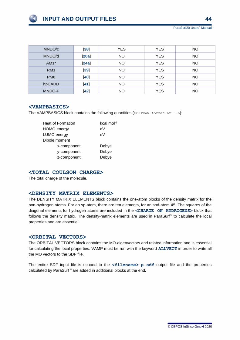
The following table gives an overview of the methods and their limitations:
Table 6 Hamiltonians and the available electrostatic and polarizability models.
Hamiltonian Reference Electrostatics Local
NAO-PC Multipole Polarizability
MNDO [20b] YES YES YES
AM1 [22] YES YES YES
PM3 [23] YES YES YES
1-Bromo-3,5-difluorobenzene
OMVAMP81A04250313563D 1 0.00000 0.00000 0
12 12 0 0 0 0 1 V2000
-2.6274 0.2410 0.0003 F
-1.2738 0.2410 0.0003 C
-0.5810 1.4623 0.0003 C
0.8231 1.4389 0.0003 C
1.5096 2.6055 0.0004 F
1.5266 0.2198 0.0001 C
0.8142 -0.9793 0.0001 C
1.7431 -2.6055 -0.0004 Br
-0.5805 -0.9840 0.0002 C
-1.1264 2.4167 -0.0003 H
2.6274 0.2339 0.0003 H
-1.1515 -1.9253 0.0001 H
1 2 1
2 3 4
3 4 4
4 5 1
4 6 4
6 7 4
7 8 1
2 9 4
7 9 4
3 10 1
6 11 1
9 12 1
M END
INPUT AND OUTPUT FILES 44
ParaSurf20 Users´ Manual
© CEPOS InSilico GmbH 2020
MNDO/c [38] YES YES NO
MNDO/d [20a] NO YES NO
AM1* [24a] NO YES NO
RM1 [39] NO YES NO
PM6 [40] NO YES NO
hpCADD [41] NO YES NO
MNDO-F [42] NO YES NO
<VAMPBASICS> The VAMPBASICS block contains the following quantities (FORTRAN format 6f13.6):
Heat of Formation kcal mol-1
HOMO energy eV
LUMO energy eV
Dipole moment
x-component Debye
y-component Debye
z-component Debye
<TOTAL COULSON CHARGE> The total charge of the molecule.
<DENSITY MATRIX ELEMENTS> The DENSITY MATRIX ELEMENTS block contains the one-atom blocks of the density matrix for the
non-hydrogen atoms. For an sp-atom, there are ten elements, for an spd-atom 45. The squares of the
diagonal elements for hydrogen atoms are included in the <CHARGE ON HYDROGENS> block that
follows the density matrix. The density-matrix elements are used in ParaSurf™ to calculate the local
properties and are essential.
<ORBITAL VECTORS> The ORBITAL VECTORS block contains the MO-eigenvectors and related information and is essential
for calculating the local properties. VAMP must be run with the keyword ALLVECT in order to write all
the MO vectors to the SDF file.
The entire SDF input file is echoed to the <filename>_p.sdf output file and the properties
calculated by ParaSurf™ are added in additional blocks at the end.
INPUT AND OUTPUT FILES 45
ParaSurf20 Users´ Manual
© CEPOS InSilico GmbH 2020
3.2.1 Multi-structure SD-files
ParaSurf™ can read SD-files containing more than one molecule (e.g. those produced by
EMPIRE™) and process them in one run. Multiple SDF files can also be contained in the input list
file if used. The command-line arguments apply to each molecule in the SD-file and the same
semiempirical Hamiltonian must be used for each molecule or an error message will be printed
and the program terminated.
As part of this enhancement, ParaSurf™ can use SD-files that do not contain the one-atom blocks
of the density matrix explicitly. Thus, SD-files that only contain the molecular-orbital Eigenvectors
and Eigenvalues give full ParaSurf™ functionality within the previous restrictions that:
• Polarisabilities are not yet available for Hamiltonians that use d-orbitals (MNDO/d and
AM1*).
• NAO-PC electrostatics are only available if the NAO-PCs are present in the SD-file.
Multipole electrostatics are available for all Hamiltonians.
The output SD-file written by ParaSurf™ also contains multiple molecules as in the input file. Other
ParaSurf™ output files (.asd, .vmp etc.) are also concatenated.
Multiple SD-files can be used with a SIM file exactly as single molecules.
3.3 The Cepos MOPAC 6.sdf file as input
Cepos Mopac 6 writes an .sdf file containing the above blocks with the exception that the
MOPACBASICS block replaces VAMPBASICS. No additional keywords are required to request the
correct .sdf output for ParaSurf™.
3.4 The <Hamiltonian>.par file
The file <Hamiltonian>.par is used by EMPIRE to define the named Hamiltonian and elements and
supply the parameters. This file is also used by ParaSurf™ for the same purpose. The <Hamiltonian>.par
file is not necessary if an EMPIRE™ .vwf file is used as input.
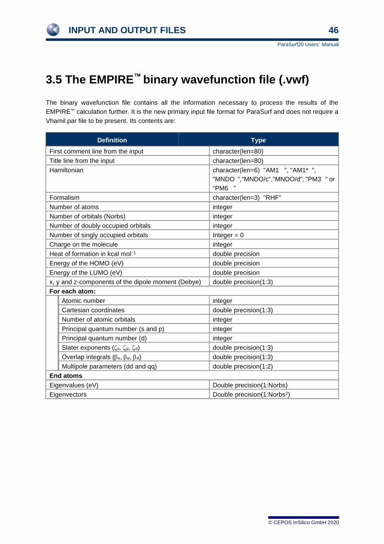
INPUT AND OUTPUT FILES 46
ParaSurf20 Users´ Manual
© CEPOS InSilico GmbH 2020
3.5 The EMPIRE™ binary wavefunction file (.vwf)
The binary wavefunction file contains all the information necessary to process the results of the
EMPIRE™ calculation further. It is the new primary input file format for ParaSurf and does not require a
Vhamil.par file to be present. Its contents are:
Definition Type
First comment line from the input character(len=80)
Title line from the input character(len=80)
Hamiltonian character(len=6) "AM1 ", "AM1* ",
"MNDO ","MNDO/c","MNDO/d", "PM3 " or
"PM6 "
Formalism character(len=3) "RHF"
Number of atoms integer
Number of orbitals (Norbs) integer
Number of doubly occupied orbitals integer
Number of singly occupied orbitals Integer = 0
Charge on the molecule integer
Heat of formation in kcal mol−1 double precision
Energy of the HOMO (eV) double precision
Energy of the LUMO (eV) double precision
x, y and z-components of the dipole moment (Debye) double precision(1:3)
For each atom:
Atomic number integer
Cartesian coordinates double precision(1:3)
Number of atomic orbitals integer
Principal quantum number (s and p) integer
Principal quantum number (d) integer
Slater exponents (s, p, d) double precision(1:3)
Overlap integrals (s, p, d) double precision(1:3)
Multipole parameters (dd and qq) double precision(1:2)
End atoms
Eigenvalues (eV) Double precision(1:Norbs)
Eigenvectors Double precision(1:Norbs2)

INPUT AND OUTPUT FILES 47
ParaSurf20 Users´ Manual
© CEPOS InSilico GmbH 2020
3.6 The ParaSurf™ output file
The ParaSurf™ output file provides the user with information about the calculation and the results. It is,
however, not intended as the primary means of communication between ParaSurf™ and other programs.
Thus, the essential information contained in the output file is also available from the ParaSurf™ output
.sdf file.
3.6.1 For a spherical-harmonic surface
Figure 14 shows the output for a calculation using the options surf=wrap fit=sphh
translate for trimethoprim, 1.
ParaSurf™ output for trimethoprim, 1, using a spherical-harmonic surface
<> ParaSurf'20, Revision 518
<> Copyright (c) 2006-2020 Cepos InSilico GmbH. All rights reserved.
<> Input = 02-trimethoprim_e.h5
<> Program options :
Using shrink-wrap isocontour surface
Fitting surface to spherical harmonics
Translations for spherical-harmonic fits: 1 step of 0.5000 Angstrom in each
direction.
Using an isodensity surface contour
Isodensity value = 0.5000E-03 electrons/Angstrom**3
Triangulation mesh = 0.20 Angstrom
Using multipole electrostatics
<<>> Molecule 1 of 1 (molecule 1 of file 1) <<>>
<> AM1 calculation for Trimethoprim
<> Translated spherical-harmonic fits:
dx dy dz rmsd
0.0000 0.0000 0.0000 0.3827
0.5000 0.0000 0.0000 0.5516
-0.5000 0.0000 0.0000 0.4939
0.0000 0.5000 0.0000 0.5333
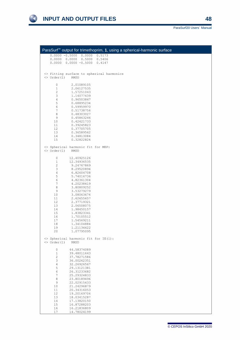
INPUT AND OUTPUT FILES 48
ParaSurf20 Users´ Manual
© CEPOS InSilico GmbH 2020
ParaSurf™ output for trimethoprim, 1, using a spherical-harmonic surface
0.0000 -0.5000 0.0000 0.5173
0.0000 0.0000 0.5000 0.5406
0.0000 0.0000 -0.5000 0.4147
<> Fitting surface to spherical harmonics
<> Order(l) RMSD
0 2.01089105
1 2.06127535
2 1.57251043
3 1.14077439
4 0.96503847
5 0.68895234
6 0.59959970
7 0.51738756
8 0.48303027
9 0.45863246
10 0.42421733
11 0.39245823
12 0.37705705
13 0.36589562
14 0.34813084
15 0.32822824
<> Spherical harmonic fit for MEP:
<> Order(l) RMSD
0 12.40925126
1 12.34936535
2 9.24767869
3 8.29520894
4 6.82604708
5 5.74016736
6 4.82361304
7 4.20238419
8 3.80809252
9 3.53279279
10 3.08063674
11 2.62655657
12 2.37719321
13 2.06508075
14 1.98450157
15 1.83823341
16 1.70105512
17 1.54569211
18 1.34104884
19 1.21134422
20 1.07795095
<> Spherical harmonic fit for IE(l):
<> Order(l) RMSD
0 44.58374089
1 39.48011643
2 37.78271586
3 36.00262351
4 32.26926567
5 29.13121381
6 26.31233682
7 25.29324833
8 23.80189496
9 22.02915433
10 21.24296879
11 20.34316053
12 19.20169704
13 18.03415287
14 17.13820150
15 16.87288203
16 16.21836809
17 14.78024199
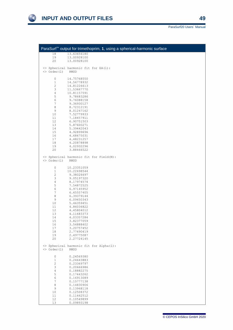
INPUT AND OUTPUT FILES 49
ParaSurf20 Users´ Manual
© CEPOS InSilico GmbH 2020
ParaSurf™ output for trimethoprim, 1, using a spherical-harmonic surface
18 13.63656180
19 13.00928100
20 13.00928100
<> Spherical harmonic fit for EA(l):
<> Order(l) RMSD
0 14.75768550
1 14.56778932
2 14.81226613
3 11.53667770
4 10.81157591
5 9.78683286
6 9.76088158
7 9.36930127
8 8.72312191
9 8.01247162
10 7.52779933
11 7.18457911
12 6.90751503
13 5.87600271
14 5.39442043
15 4.92899696
16 4.68675031
17 4.48231257
18 4.20878898
19 4.02932296
20 3.88466522
<> Spherical harmonic fit for Field(N):
<> Order(l) RMSD
0 10.23351059
1 10.22698544
2 9.38026697
3 9.05197320
4 8.17974574
5 7.54872525
6 6.97145952
7 6.65557405
8 6.39379144
9 6.09450343
10 5.46359451
11 4.86036822
12 4.45804012
13 4.11683373
14 4.03357284
15 3.82377059
16 3.54888402
17 3.20757452
18 2.77490419
19 2.49775087
20 2.27724145
<> Spherical harmonic fit for Alpha(l):
<> Order(l) RMSD
0 0.24569380
1 0.24643883
2 0.23369797
3 0.20666986
4 0.18882275
5 0.17443262
6 0.16913089
7 0.15777138
8 0.14830906
9 0.13948118
10 0.12508372
11 0.11462512
12 0.10549899
13 0.09893198

INPUT AND OUTPUT FILES 50
ParaSurf20 Users´ Manual
© CEPOS InSilico GmbH 2020
ParaSurf™ output for trimethoprim, 1, using a spherical-harmonic surface
14 0.09585367
15 0.09003283
16 0.08226668
17 0.07498713
18 0.06877556
19 0.06575083
20 0.06285391
<> Property ranges:
Density : 0.1002E-03 to 0.1834E-02
IE(l) : 325.71 to 554.60
EA(l) : -112.62 to -29.19
MEP : -50.24 to 19.03
Alpha(l) : 0.2167 to 1.5078
Field(N) : -52.88 to 19.79
<> Descriptors :
Dipole moment : 1.2492 Debye
Dipolar density : 0.2450E-02 Debye.Angstrom**-3
Molecular pol. : 31.2348 Angstrom**3
Molecular weight : 290.32
Globularity : 0.7559
Total surface area : 408.30 Angstrom**2
Molecular volume : 509.82 Angstrom**3
Most positive MEP : 19.03 kcal/mol
Most negative MEP : -50.24 kcal/mol
Mean +ve MEP : 6.29 kcal/mol
Mean -ve MEP : -11.87 kcal/mol
Mean MEP : -2.38 kcal/mol
MEP range : 69.26 kcal/mol
MEP +ve Variance : 15.51 (kcal/mol)**2
MEP -ve Variance : 133.18 (kcal/mol)**2
MEP total variance : 148.69 (kcal/mol)**2
MEP balance parameter: 0.0934
MEP balance*variance : 13.8910 kcal/mol
MEP skewness : -1.3150
MEP kurtosis : 1.5930
Integral MEP : -823.441 kcal.Angstrom**2/mol
Maximum IE(l) : 554.60 kcal/mol
Minimum IE(l) : 325.71 kcal/mol
Mean IE(l) : 422.42 kcal/mol
IE(l) range : 228.89 kcal/mol
IE(l) variance : 1947.78 (kcal/mol)**2
IE(l) skewness : 0.6852
IE(l) kurtosis : -0.3191
Integral IE(l) : 7450.24 eV.Angstrom**2
Maximum EA(l) : -29.19 kcal/mol
Minimum EA(l) : -112.62 kcal/mol
Mean +ve EA(l) : 0.00 kcal/mol
Mean -ve EA(l) : -93.26 kcal/mol
Mean EA(l) : -93.26 kcal/mol
EA(l) range : 83.43 kcal/mol
EA(l) +ve variance : 0.00 (kcal/mol)**2
EA(l) -ve variance : 203.22 (kcal/mol)**2
EA(l) total variance : 203.22 (kcal/mol)**2
EA(l) skewness : 1.5615
EA(l) kurtosis : 3.0492
Integral EA(l) : -1647.43 eV.Angstrom**2
EA(l) balance param. : 0.0000
Fraction pos. EA(l) : 0.0000 ( = 0.00 Angstrom**2)
Max. local Eneg. : 234.17 kcal/mol
Min. local Eneg. : 113.01 kcal/mol
Mean local Eneg. : 164.58 kcal/mol
Local Eneg. range : 121.15 kcal/mol
Local Eneg. variance : 453.89 (kcal/mol)**2
Local Eneg. skewness : 0.66
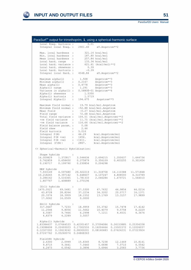
INPUT AND OUTPUT FILES 51
ParaSurf20 Users´ Manual
© CEPOS InSilico GmbH 2020
ParaSurf™ output for trimethoprim, 1, using a spherical-harmonic surface
Local Eneg. kurtosis : 0.01
Integral local Eneg. : 2901.40 eV.Angstrom**2
Max. local hardness : 321.14 kcal/mol
Min. local hardness : 187.80 kcal/mol
Mean local hardness : 257.84 kcal/mol
Local hard. range : 133.34 kcal/mol
Local hard. variance : 621.61 (kcal/mol)**2
Local hard. skewness : 0.39
Local hard. kurtosis : -0.39
Integral local Hard. : 4548.84 eV.Angstrom**2
Maximum alpha(l) : 1.508 Angstrom**3
Minimum alpha(l) : 0.2167 Angstrom**3
Mean alpha(l) : 0.4778 Angstrom**3
Alpha(l) range : 1.291 Angstrom**3
Variance in alpha(l) : 0.5880E-01 Angstrom**6
Alpha(l) skewness : 1.5350
Alpha(l) kurtosis : 1.5719
Integral Alpha(l) : 194.675 Angstrom**5
Maximum field normal : 19.79 kcal/mol.Angstrom
Minimum field normal : -52.88 kcal/mol.Angstrom
Mean field : -0.27 kcal/mol.Angstrom
Field range : 72.68 kcal/mol.Angstrom
Total field variance : 104.51 (kcal/mol.Angstrom)**2
+ve field variance : 11.75 (kcal/mol.Angstrom)**2
-ve field variance : 116.66 (kcal/mol.Angstrom)**2
Field balance param. : 0.08
Field skew : 2.46
Field kurtosis : 5.016
Integral F(N) : 44.29 kcal.Angstrom/mol
Integral F(N +ve) : 1456. kcal.Angstrom/mol
Integral F(N -ve) : -1411. kcal.Angstrom/mol
Integral |F(N)| : 2867. kcal.Angstrom/mol
<> Spherical-Harmonic Hybridization:
Shape hybrids :
16.009829 1.372817 3.546636 2.694215 1.350637 1.644736
0.762859 0.658450 0.375879 0.356109 0.403255 0.301454
0.190717 0.199790 0.230856 0.204298
MEP hybrids :
7.933149 4.597680 29.922219 11.318758 14.110388 11.571848
10.218265 8.397142 5.648607 4.107247 4.808593 4.310789
3.286162 3.516365 1.781333 2.046284 1.479721 1.564010
1.807767 1.408889 1.370196
IE(l) hybrids :
1475.0521 69.5481 57.5300 47.7632 44.9854 44.0214
43.8728 28.8264 37.2234 34.3202 20.0717 16.1371
20.3376 18.3959 18.1552 13.1769 13.3157 17.9899
17.9262 16.0509 0.0000
EA(l) hybrids :
317.0647 7.7233 18.9959 33.3742 15.7478 17.4142
11.2546 9.8056 11.5662 10.4079 9.5758 8.2229
6.5587 9.7466 6.2998 7.1211 4.4531 4.3676
4.8379 4.2289 3.5057
Alpha(l) hybrids :
1.83384637 0.07664533 0.42301457 0.37094086 0.26153885 0.25356338
0.19288699 0.22493023 0.17302555 0.16204464 0.15501572 0.12026037
0.12327202 0.10619242 0.08300201 0.08160683 0.07624231 0.07223924
0.07247762 0.05260074 0.04868363
Field(N) hybrids :
2.6300 2.0999 15.8345 8.7238 12.1449 10.8141
9.8715 9.3441 7.0440 5.6698 7.0710 6.5542
6.2473 6.0542 3.3896 3.6944 3.2583 3.7736

INPUT AND OUTPUT FILES 52
ParaSurf20 Users´ Manual
© CEPOS InSilico GmbH 2020
ParaSurf™ output for trimethoprim, 1, using a spherical-harmonic surface
4.2053 3.4600 2.9092
<> Standard rotationally invariant fingerprint:(L. Mavridis, B. D. Hudson
and D. W. Ritchie, J. Chem. Inf. Model., 2007, 47, 1787-1796.)
4.00123 1.17167 1.88325 1.64141 1.16217
1.28247 0.873418 2.81658 2.14422 5.47012
3.36434 3.75638 3.40174 3.19660 2.89778
2.37668 2.02663 2.19285 2.07624 1.81278
38.4064 8.33955 7.58486 6.91109 6.70712
6.63486 6.62365 17.8063 2.77909 4.35843
5.77704 3.96835 4.17304 3.35478 1.35420
0.276849 0.650396 0.609049 0.511409 0.503551
0.439189 1.62172 1.44910 3.97925 2.95360
3.48496 3.28849 3.14190 3.05682 2.65406
2.38113 2.65914 2.56012 2.49946
<> Atomic surface properties:
Atom Area MEP IE(l) EA(l) mean Field(N) Eneg(L) Hard(L)
max min max min max min pol. max min max min max min
C 1 1.190 -4.98 -24.62 474.52 440.67 -84.14 -97.48 0.695 -0.83 -19.62 195.19 171.59 279.33 268.79
O 2 3.298 -15.19 -48.76 483.54 395.34 -68.95 -88.24 1.012 -10.65 -35.98 204.70 153.55 278.84 238.13
C 3 5.583 2.77 -42.28 473.04 343.33 -31.90 -102.55 0.844 3.13 -23.13 198.97 137.79 274.58 192.50
C 4 2.301 -1.10 -11.02 420.69 358.04 -47.63 -88.64 0.765 0.11 -7.47 167.89 147.82 252.80 202.83
C 5 1.315 -2.84 -11.05 443.61 381.75 -69.71 -93.96 0.779 -2.54 -6.76 174.83 152.50 268.78 226.30
C 6 0.000
C 7 1.851 -1.56 -11.81 420.68 353.37 -51.21 -93.16 0.865 -0.54 -7.17 169.84 141.72 250.85 207.23
C 8 6.599 0.72 -22.08 435.15 362.30 -35.17 -99.13 0.778 2.08 -15.48 176.42 150.10 258.90 203.03
N 9 7.657 -9.91 -40.75 444.04 328.38 -82.14 -109.12 1.186 -10.05 -52.88 175.09 113.01 269.73 214.66
C 10 10.569 5.93 -23.31 493.59 388.55 -37.04 -96.74 0.790 4.70 -15.88 208.37 154.52 288.56 213.60
N 11 1.649 -14.32 -23.08 511.29 446.84 -62.99 -82.88 0.792 -16.62 -22.27 216.19 190.15 295.10 254.92
N 12 6.596 -9.44 -39.65 444.88 325.71 -80.14 -106.62 1.030 -10.90 -51.98 172.09 115.02 274.06 206.65
C 13 7.455 4.99 -25.73 511.75 366.67 -34.09 -96.81 0.812 6.63 -21.17 215.41 152.09 296.33 201.39
N 14 1.811 -14.21 -22.59 489.46 443.66 -66.68 -87.81 0.801 -18.52 -29.45 206.00 184.50 285.59 256.30
C 15 4.922 -0.84 -11.94 434.32 358.04 -52.10 -100.46 0.747 2.70 -9.38 173.09 145.62 261.23 205.09
C 16 5.487 -2.04 -37.62 476.46 346.23 -29.19 -99.46 0.820 2.98 -22.97 200.41 139.18 276.05 187.80
O 17 0.967 -23.74 -38.38 475.29 409.49 -71.32 -88.43 0.959 -11.17 -33.70 198.67 165.28 276.61 240.88
C 18 0.868 9.69 -22.92 505.07 434.72 -83.99 -98.88 0.689 5.54 -12.51 207.97 167.92 297.10 266.80
C 19 5.387 -1.42 -46.07 485.07 325.82 -36.31 -103.12 1.007 -5.14 -29.69 201.93 133.19 286.11 189.83
O 20 4.532 -34.23 -50.24 477.49 372.31 -73.80 -95.93 1.085 -18.29 -43.77 201.85 143.15 279.41 228.83
C 21 1.026 -20.40 -37.72 465.11 425.53 -93.35 -109.78 0.771 -4.76 -21.37 184.51 157.88 280.63 267.65
H 22 24.371 9.65 -29.37 508.62 383.66 -87.46 -97.42 0.402 6.63 -16.31 209.38 145.02 299.24 238.64
H 23 17.654 12.03 -11.10 503.81 382.61 -76.92 -97.29 0.369 7.51 -8.88 207.26 145.68 296.55 236.88
H 24 18.561 11.71 -14.41 502.89 382.82 -77.33 -96.23 0.366 6.31 -3.93 206.55 145.37 296.34 237.45
H 25 6.426 12.26 0.37 450.62 398.89 -84.39 -99.10 0.374 9.18 -4.08 178.64 152.19 271.98 243.06
H 26 14.980 8.86 -4.48 463.19 374.77 -88.80 -102.50 0.381 6.24 -3.26 182.46 139.03 281.27 235.75
H 27 14.448 8.05 -15.74 465.97 374.03 -85.10 -102.82 0.383 5.60 -6.12 190.43 137.77 279.85 236.26
H 28 18.509 9.52 -25.29 438.30 391.89 -70.52 -102.74 0.407 8.08 -22.53 174.27 149.40 270.04 233.26
H 29 23.100 18.95 -25.76 550.92 428.60 -78.35 -111.75 0.333 19.12 -24.36 232.81 159.06 321.14 269.54
H 30 22.787 19.03 -25.69 549.09 416.55 -78.18 -111.75 0.317 19.79 -23.61 234.17 154.02 320.16 262.53
H 31 22.912 15.18 -25.52 554.60 420.68 -77.19 -112.62 0.314 13.90 -26.29 234.03 156.03 320.57 264.64
H 32 8.917 14.54 -11.91 552.72 397.81 -78.67 -104.80 0.356 14.61 -19.29 232.59 149.52 320.14 248.30
H 33 6.289 10.08 -4.73 441.21 384.47 -73.09 -98.76 0.443 8.53 -6.17 172.35 147.80 268.86 228.78
H 34 23.000 9.47 -23.20 498.60 384.30 -87.92 -99.94 0.374 6.36 -15.55 204.59 145.05 294.02 238.59
H 35 18.461 9.75 -15.62 500.37 380.66 -73.15 -96.26 0.380 6.52 -6.88 205.63 145.27 294.74 231.11
H 36 18.392 9.64 -6.06 502.36 382.30 -80.87 -97.20 0.382 8.17 -12.01 206.73 145.23 295.62 237.07
H 37 24.578 3.25 -31.68 487.58 370.62 -99.57 -109.64 0.393 3.95 -22.88 192.71 133.07 294.87 237.54
H 38 17.255 2.55 -34.54 495.64 367.12 -87.21 -109.16 0.387 2.36 -21.42 196.50 130.27 299.14 236.79
H 39 21.194 2.66 -35.54 490.73 358.95 -87.35 -108.59 0.375 2.69 -25.26 194.18 130.18 296.55 226.34
Total 402.899
<> Stationary points on the molecular surface
(A. Jakobi, H. Mauser and T. Clark, J. Mol. Model., 2008, 14, 547-558)
x y z value
<> 9 MEP Maxima :
-2.0942 -1.9102 1.9957 14.49
1.9307 2.6574 -1.9069 10.08

INPUT AND OUTPUT FILES 53
ParaSurf20 Users´ Manual
© CEPOS InSilico GmbH 2020
ParaSurf™ output for trimethoprim, 1, using a spherical-harmonic surface
4.2002 2.2888 -1.9834 9.694
2.3854 4.1407 4.8110 19.03
1.4638 5.7587 5.4768 12.76
-1.4292 -1.7903 3.3076 15.18
-0.1036 3.5081 -2.4659 9.520
-4.5243 -1.3404 -0.6240 12.26
1.9418 3.3249 5.3086 17.29
<> 5 MEP Minima :
0.6146 5.8475 1.0368 -40.75
0.0000 -4.3477 -2.5240 -50.24
-1.4714 2.3729 4.3877 -39.65
0.8011 -3.6508 -3.4297 -45.17
2.6849 -2.2207 -2.9411 -38.38
<> 7 IEL Maxima :
-3.0426 -1.2047 2.7459 554.6
0.2652 -0.8162 2.3579 538.2
-0.1428 -1.3588 2.3664 539.8
-1.9645 -1.8861 2.7449 546.7
-0.9455 -1.8557 2.5130 543.5
2.1929 5.4999 5.4576 550.9
1.0590 5.7160 5.3689 550.8
<> 4 IEL Minima :
-1.3070 2.2638 4.5277 325.7
0.2228 -2.1196 -3.6914 325.8
-0.2633 1.6255 4.6957 332.6
0.9079 5.7325 1.0276 328.4
<> 4 EAL Maxima :
-2.9082 2.6186 2.2718 -34.09
-2.2331 4.3871 0.4313 -35.17
-1.0954 -2.0486 -3.3583 -31.90
0.4612 -0.8006 -3.6052 -29.19
<> 8 EAL Minima :
0.2957 -5.5121 -1.4811 -109.8
1.1122 -5.2323 -3.1054 -107.1
-0.9624 -0.1287 4.9079 -112.6
2.6860 -2.4185 0.9712 -106.7
3.1807 -3.6011 -3.0614 -109.3
4.1894 -2.5658 0.2149 -106.6
0.5537 2.7843 5.8595 -111.7
1.8617 6.2852 2.3982 -111.7
<> 1 Alpha(l) Maxima :
0.9079 5.7325 1.0276 1.508
<> 43 Alpha(l) Minima :
0.1941 -0.5973 3.5619 0.2183
-2.6409 -5.9315 0.0000 0.3148
0.0000 -5.4566 0.0000 0.3504
-3.8091 2.1992 -1.6009 0.3086
-3.2197 2.3393 -2.2977 0.3049
4.7631 -0.6017 -4.0285 0.3007
2.0760 1.6769 0.7161 0.3541
-1.7867 4.6717 -1.3420 0.2992
-3.8321 1.4764 1.1019 0.3536
-3.3600 -0.9080 1.6252 0.2680
0.0000 -1.1114 3.2108 0.2167
-1.8684 -5.7502 -2.2127 0.3169
2.5579 -5.0050 1.5082 0.3071
1.3440 3.4789 -1.7415 0.3159
1.3550 2.3350 -2.7116 0.3271
-4.8886 -2.1766 0.0000 0.3252
3.1678 0.2909 -4.5678 0.2969
2.2364 1.3735 0.8283 0.3513
-2.4257 0.7858 4.4900 0.2262
-2.5222 -3.6775 1.4074 0.3005
0.1013 -3.7289 1.1773 0.3635
-1.7602 -5.9234 -1.3715 0.3158
-5.0212 -3.6481 0.5445 0.3364
-2.4804 -5.5710 -2.8511 0.3163
4.0480 -0.2121 0.7177 0.2940

INPUT AND OUTPUT FILES 54
ParaSurf20 Users´ Manual
© CEPOS InSilico GmbH 2020
ParaSurf™ output for trimethoprim, 1, using a spherical-harmonic surface
2.4150 5.0622 5.1801 0.2208
3.0687 2.6190 -0.8974 0.3555
-0.4681 4.4658 5.9019 0.2284
4.6450 -3.9692 0.2672 0.3134
4.4727 -3.4302 -1.7843 0.3238
-4.8830 -1.8743 -1.9116 0.3160
-3.9257 -0.7207 -2.0799 0.3159
-3.3469 -3.7161 -3.8579 0.3006
3.5219 -6.1001 -0.6180 0.3327
3.0798 -4.7428 -3.2784 0.3042
5.4842 -1.0144 -0.7349 0.2993
5.7717 1.0662 -2.4400 0.3602
1.2319 -3.0702 1.4575 0.3175
2.0934 5.6781 2.0628 0.2653
2.5350 4.8424 2.6989 0.2363
2.0847 3.3491 4.9587 0.2218
2.6336 4.8200 3.3408 0.2302
0.3362 6.5479 2.7231 0.2359
<> 12 F(N) Maxima :
-0.5388 -1.6584 2.0781 14.28
1.1425 5.9891 5.1567 12.89
-1.6504 -1.7170 3.4430 13.58
0.3958 5.0471 6.0897 10.52
2.1544 3.5134 4.9573 17.87
-0.2643 0.4295 4.5982 11.43
-1.4216 -0.3912 4.9110 11.92
-0.0484 -1.0598 3.5334 13.59
1.9418 3.3249 5.3086 18.56
2.5160 4.5342 4.5738 14.91
2.6836 5.1541 3.8995 18.03
2.6861 5.2419 3.5888 18.51
<> 13 F(N) Minima :
-0.5249 1.6153 4.6665 -47.71
-1.3070 2.2638 4.5277 -45.59
2.8613 -2.0789 -2.9677 -31.34
-3.4166 1.0124 2.5039 -26.32
-0.7779 -4.8988 -0.4346 -30.95
-1.2132 5.3511 4.2166 -21.65
-0.6484 -4.9580 -1.1098 -31.96
0.9079 5.7325 1.0276 -50.34
0.0536 -4.2249 -2.7040 -41.20
-0.0608 1.3324 4.4423 -48.59
3.4584 -1.4319 0.1637 -12.76
-0.6374 -4.8513 -1.5489 -33.03
1.0472 -3.6236 -3.4753 -41.54
<> ParaSurf used 1.84 seconds CPU time
Figure 14 ParaSurf™ output for trimethoprim, 1, using a spherical-harmonic surface.
After printing the program options, ParaSurf19™ prints the shift in coordinates of the centre and
the RMSD fits for the surface requested by the translate option. For speed, these fits use a
lower number of surface points than the full fits that follow and are only calculated up to order six.
ParaSurf19™ then moves on to fit the calculated shrink-wrap surface at full resolution for each of
the local properties. It lists the root-mean-square deviations (RMSDs) for the surface points as a
function of the order of the spherical-harmonic expansion, first for the geometry of the surface
and then for each of the five local properties. The RMSD values give an idea of how well each
order of the spherical-harmonic expansion fits the calculated shrink-wrap surface or the relevant
property. The highest order used by ParaSurf™ is 15 for the surface itself and 20 for each property.
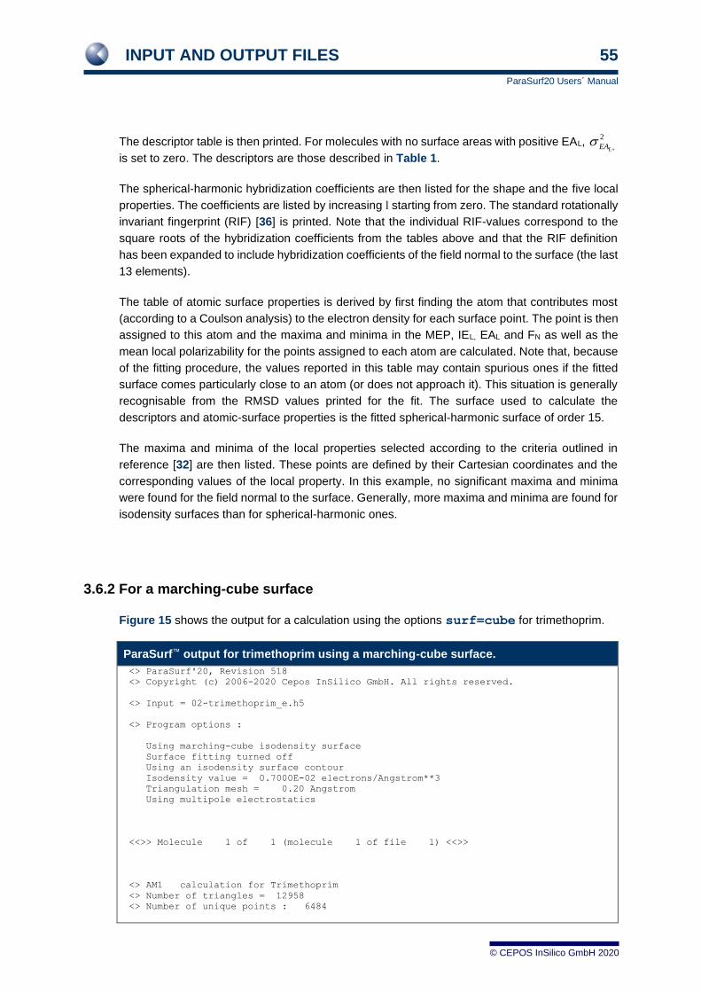
INPUT AND OUTPUT FILES 55
ParaSurf20 Users´ Manual
© CEPOS InSilico GmbH 2020
The descriptor table is then printed. For molecules with no surface areas with positive EAL,
is set to zero. The descriptors are those described in Table 1.
The spherical-harmonic hybridization coefficients are then listed for the shape and the five local
properties. The coefficients are listed by increasing l starting from zero. The standard rotationally
invariant fingerprint (RIF) [36] is printed. Note that the individual RIF-values correspond to the
square roots of the hybridization coefficients from the tables above and that the RIF definition
has been expanded to include hybridization coefficients of the field normal to the surface (the last
13 elements).
The table of atomic surface properties is derived by first finding the atom that contributes most
(according to a Coulson analysis) to the electron density for each surface point. The point is then
assigned to this atom and the maxima and minima in the MEP, IEL, EAL and FN as well as the
mean local polarizability for the points assigned to each atom are calculated. Note that, because
of the fitting procedure, the values reported in this table may contain spurious ones if the fitted
surface comes particularly close to an atom (or does not approach it). This situation is generally
recognisable from the RMSD values printed for the fit. The surface used to calculate the
descriptors and atomic-surface properties is the fitted spherical-harmonic surface of order 15.
The maxima and minima of the local properties selected according to the criteria outlined in
reference [32] are then listed. These points are defined by their Cartesian coordinates and the
corresponding values of the local property. In this example, no significant maxima and minima
were found for the field normal to the surface. Generally, more maxima and minima are found for
isodensity surfaces than for spherical-harmonic ones.
3.6.2 For a marching-cube surface
Figure 15 shows the output for a calculation using the options surf=cube for trimethoprim.
ParaSurf™ output for trimethoprim using a marching-cube surface.
<> ParaSurf'20, Revision 518
<> Copyright (c) 2006-2020 Cepos InSilico GmbH. All rights reserved.
<> Input = 02-trimethoprim_e.h5
<> Program options :
Using marching-cube isodensity surface
Surface fitting turned off
Using an isodensity surface contour
Isodensity value = 0.7000E-02 electrons/Angstrom**3
Triangulation mesh = 0.20 Angstrom
Using multipole electrostatics
<<>> Molecule 1 of 1 (molecule 1 of file 1) <<>>
<> AM1 calculation for Trimethoprim
<> Number of triangles = 12958
<> Number of unique points : 6484
2
LEA+

INPUT AND OUTPUT FILES 56
ParaSurf20 Users´ Manual
© CEPOS InSilico GmbH 2020
ParaSurf™ output for trimethoprim using a marching-cube surface.
<> Property ranges:
Density : 0.6667E-02 to 0.7293E-02
IE(l) : 313.25 to 539.63
EA(l) : -112.07 to -20.09
MEP : -64.19 to 28.40
Alpha(l) : 0.2316 to 1.5616
Field(N) : -96.24 to 62.75
<> Descriptors :
Dipole moment : 1.2492 Debye
Dipolar density : 0.4116E-02 Debye.Angstrom**-3
Molecular pol. : 31.2348 Angstrom**3
Molecular weight : 290.32
Globularity : 0.6827
Total surface area : 319.90 Angstrom**2
Molecular volume : 303.47 Angstrom**3
Most positive MEP : 28.40 kcal/mol
Most negative MEP : -64.19 kcal/mol
Mean +ve MEP : 10.18 kcal/mol
Mean -ve MEP : -19.04 kcal/mol
Mean MEP : -3.76 kcal/mol
MEP range : 92.59 kcal/mol
MEP +ve Variance : 41.22 (kcal/mol)**2
MEP -ve Variance : 267.69 (kcal/mol)**2
MEP total variance : 308.91 (kcal/mol)**2
MEP balance parameter: 0.1156
MEP balance*variance : 35.7161 kcal/mol
MEP skewness : -1.0386
MEP kurtosis : 0.6461
Integral MEP : -1123.74 kcal.Angstrom**2/mol
Maximum IE(l) : 539.63 kcal/mol
Minimum IE(l) : 313.25 kcal/mol
Mean IE(l) : 419.36 kcal/mol
IE(l) range : 226.38 kcal/mol
IE(l) variance : 1692.94 (kcal/mol)**2
IE(l) skewness : 0.5386
IE(l) kurtosis : -0.2650
Integral IE(l) : 5814.85 eV.Angstrom**2
Maximum EA(l) : -20.09 kcal/mol
Minimum EA(l) : -112.07 kcal/mol
Mean +ve EA(l) : 0.00 kcal/mol
Mean -ve EA(l) : -86.90 kcal/mol
Mean EA(l) : -86.90 kcal/mol
EA(l) range : 91.99 kcal/mol
EA(l) +ve variance : 0.00 (kcal/mol)**2
EA(l) -ve variance : 363.26 (kcal/mol)**2
EA(l) total variance : 363.26 (kcal/mol)**2
EA(l) skewness : 1.3467
EA(l) kurtosis : 1.2533
Integral EA(l) : -1215.64 eV.Angstrom**2
EA(l) balance param. : 0.0000
Fraction pos. EA(l) : 0.0000 ( = 0.00 Angstrom**2)
Max. local Eneg. : 231.46 kcal/mol
Min. local Eneg. : 108.12 kcal/mol
Mean local Eneg. : 166.23 kcal/mol
Local Eneg. range : 123.34 kcal/mol
Local Eneg. variance : 417.45 (kcal/mol)**2
Local Eneg. skewness : 0.33
Local Eneg. kurtosis : -0.11
Integral local Eneg. : 2299.60 eV.Angstrom**2
Max. local hardness : 312.11 kcal/mol
Min. local hardness : 191.60 kcal/mol
Mean local hardness : 253.13 kcal/mol
Local hard. range : 120.51 kcal/mol
Local hard. variance : 610.65 (kcal/mol)**2
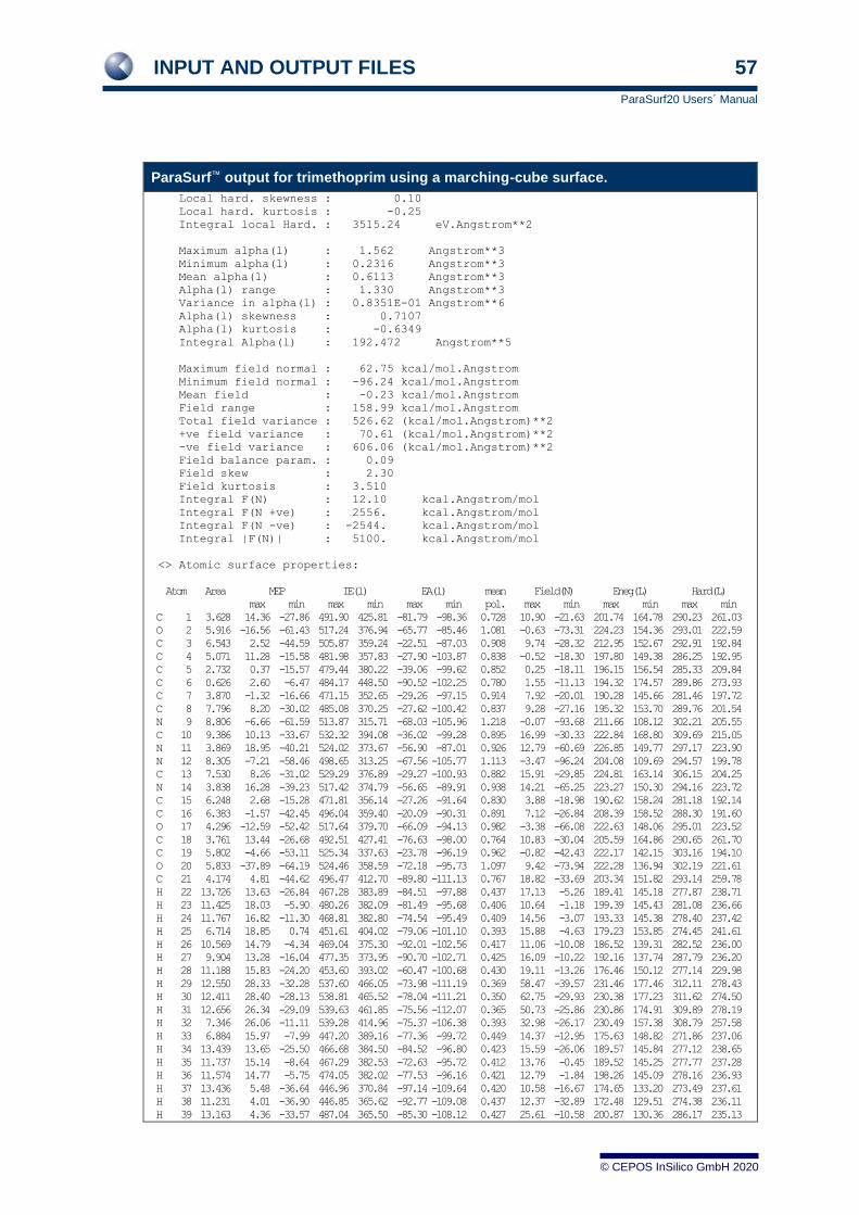
INPUT AND OUTPUT FILES 57
ParaSurf20 Users´ Manual
© CEPOS InSilico GmbH 2020
ParaSurf™ output for trimethoprim using a marching-cube surface.
Local hard. skewness : 0.10
Local hard. kurtosis : -0.25
Integral local Hard. : 3515.24 eV.Angstrom**2
Maximum alpha(l) : 1.562 Angstrom**3
Minimum alpha(l) : 0.2316 Angstrom**3
Mean alpha(l) : 0.6113 Angstrom**3
Alpha(l) range : 1.330 Angstrom**3
Variance in alpha(l) : 0.8351E-01 Angstrom**6
Alpha(l) skewness : 0.7107
Alpha(l) kurtosis : -0.6349
Integral Alpha(l) : 192.472 Angstrom**5
Maximum field normal : 62.75 kcal/mol.Angstrom
Minimum field normal : -96.24 kcal/mol.Angstrom
Mean field : -0.23 kcal/mol.Angstrom
Field range : 158.99 kcal/mol.Angstrom
Total field variance : 526.62 (kcal/mol.Angstrom)**2
+ve field variance : 70.61 (kcal/mol.Angstrom)**2
-ve field variance : 606.06 (kcal/mol.Angstrom)**2
Field balance param. : 0.09
Field skew : 2.30
Field kurtosis : 3.510
Integral F(N) : 12.10 kcal.Angstrom/mol
Integral F(N +ve) : 2556. kcal.Angstrom/mol
Integral F(N -ve) : -2544. kcal.Angstrom/mol
Integral |F(N)| : 5100. kcal.Angstrom/mol
<> Atomic surface properties:
Atom Area MEP IE(l) EA(l) mean Field(N) Eneg(L) Hard(L)
max min max min max min pol. max min max min max min
C 1 3.628 14.36 -27.86 491.90 425.81 -81.79 -98.36 0.728 10.90 -21.63 201.74 164.78 290.23 261.03
O 2 5.916 -16.56 -61.43 517.24 376.94 -65.77 -85.46 1.081 -0.63 -73.31 224.23 154.36 293.01 222.59
C 3 6.543 2.52 -44.59 505.87 359.24 -22.51 -87.03 0.908 9.74 -28.32 212.95 152.67 292.91 192.84
C 4 5.071 11.28 -15.58 481.98 357.83 -27.90 -103.87 0.838 -0.52 -18.30 197.80 149.38 286.25 192.95
C 5 2.732 0.37 -15.57 479.44 380.22 -39.06 -99.62 0.852 0.25 -18.11 196.15 156.54 285.33 209.84
C 6 0.626 2.60 -6.47 484.17 448.50 -90.52 -102.25 0.780 1.55 -11.13 194.32 174.57 289.86 273.93
C 7 3.870 -1.32 -16.66 471.15 352.65 -29.26 -97.15 0.914 7.92 -20.01 190.28 145.66 281.46 197.72
C 8 7.796 8.20 -30.02 485.08 370.25 -27.62 -100.42 0.837 9.28 -27.16 195.32 153.70 289.76 201.54
N 9 8.806 -6.66 -61.59 513.87 315.71 -68.03 -105.96 1.218 -0.07 -93.68 211.66 108.12 302.21 205.55
C 10 9.386 10.13 -33.67 532.32 394.08 -36.02 -99.28 0.895 16.99 -30.33 222.84 168.80 309.69 215.05
N 11 3.869 18.95 -40.21 524.02 373.67 -56.90 -87.01 0.926 12.79 -60.69 226.85 149.77 297.17 223.90
N 12 8.305 -7.21 -58.46 498.65 313.25 -67.56 -105.77 1.113 -3.47 -96.24 204.08 109.69 294.57 199.78
C 13 7.530 8.26 -31.02 529.29 376.89 -29.27 -100.93 0.882 15.91 -29.85 224.81 163.14 306.15 204.25
N 14 3.838 16.28 -39.23 517.42 374.79 -56.65 -89.91 0.938 14.21 -65.25 223.27 150.30 294.16 223.72
C 15 6.248 2.68 -15.28 471.81 356.14 -27.26 -91.64 0.830 3.88 -18.98 190.62 158.24 281.18 192.14
C 16 6.383 -1.57 -42.45 496.04 359.40 -20.09 -90.31 0.891 7.12 -26.84 208.39 158.52 288.30 191.60
O 17 4.296 -12.59 -52.42 517.64 379.70 -66.09 -94.13 0.982 -3.38 -66.08 222.63 148.06 295.01 223.52
C 18 3.761 13.44 -26.68 492.51 427.41 -76.63 -98.00 0.764 10.83 -30.04 205.59 164.86 290.65 261.70
C 19 5.802 -4.66 -53.11 525.34 337.63 -23.78 -96.19 0.962 -0.82 -42.43 222.17 142.15 303.16 194.10
O 20 5.833 -37.89 -64.19 524.46 358.59 -72.18 -95.73 1.097 9.42 -73.94 222.28 136.94 302.19 221.61
C 21 4.174 4.81 -44.62 496.47 412.70 -89.80 -111.13 0.767 18.82 -33.69 203.34 151.82 293.14 259.78
H 22 13.726 13.63 -26.84 467.28 383.89 -84.51 -97.88 0.437 17.13 -5.26 189.41 145.18 277.87 238.71
H 23 11.425 18.03 -5.90 480.26 382.09 -81.49 -95.68 0.406 10.64 -1.18 199.39 145.43 281.08 236.66
H 24 11.767 16.82 -11.30 468.81 382.80 -74.54 -95.49 0.409 14.56 -3.07 193.33 145.38 278.40 237.42
H 25 6.714 18.85 0.74 451.61 404.02 -79.06 -101.10 0.393 15.88 -4.63 179.23 153.85 274.45 241.61
H 26 10.569 14.79 -4.34 469.04 375.30 -92.01 -102.56 0.417 11.06 -10.08 186.52 139.31 282.52 236.00
H 27 9.904 13.28 -16.04 477.35 373.95 -90.70 -102.71 0.425 16.09 -10.22 192.16 137.74 287.79 236.20
H 28 11.188 15.83 -24.20 453.60 393.02 -60.47 -100.68 0.430 19.11 -13.26 176.46 150.12 277.14 229.98
H 29 12.550 28.33 -32.28 537.60 466.05 -73.98 -111.19 0.369 58.47 -39.57 231.46 177.46 312.11 278.43
H 30 12.411 28.40 -28.13 538.81 465.52 -78.04 -111.21 0.350 62.75 -29.93 230.38 177.23 311.62 274.50
H 31 12.656 26.34 -29.09 539.63 461.85 -75.56 -112.07 0.365 50.73 -25.86 230.86 174.91 309.89 278.19
H 32 7.346 26.06 -11.11 539.28 414.96 -75.37 -106.38 0.393 32.98 -26.17 230.49 157.38 308.79 257.58
H 33 6.884 15.97 -7.99 447.20 389.16 -77.36 -99.72 0.449 14.37 -12.95 175.63 148.82 271.86 237.06
H 34 13.439 13.65 -25.50 466.68 384.50 -84.52 -96.80 0.423 15.59 -26.06 189.57 145.84 277.12 238.65
H 35 11.737 15.14 -8.64 467.29 382.53 -72.63 -95.72 0.412 13.76 -0.45 189.52 145.25 277.77 237.28
H 36 11.574 14.77 -5.75 474.05 382.02 -77.53 -96.16 0.421 12.79 -1.84 198.26 145.09 278.16 236.93
H 37 13.436 5.48 -36.64 446.96 370.84 -97.14 -109.64 0.420 10.58 -16.67 174.65 133.20 273.49 237.61
H 38 11.231 4.01 -36.90 446.85 365.62 -92.77 -109.08 0.437 12.37 -32.89 172.48 129.51 274.38 236.11
H 39 13.163 4.36 -33.57 487.04 365.50 -85.30 -108.12 0.427 25.61 -10.58 200.87 130.36 286.17 235.13
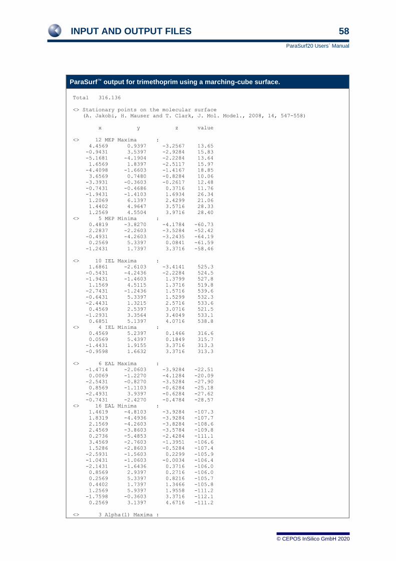
INPUT AND OUTPUT FILES 58
ParaSurf20 Users´ Manual
© CEPOS InSilico GmbH 2020
ParaSurf™ output for trimethoprim using a marching-cube surface.
Total 316.136
<> Stationary points on the molecular surface
(A. Jakobi, H. Mauser and T. Clark, J. Mol. Model., 2008, 14, 547-558)
x y z value
<> 12 MEP Maxima :
4.4569 0.9397 -3.2567 13.65
-0.9431 3.5397 -2.9284 15.83
-5.1681 -4.1904 -2.2284 13.64
1.6569 1.8397 -2.5117 15.97
-4.4098 -1.6603 -1.4167 18.85
3.6569 0.7480 -0.8284 10.06
-3.3931 -0.3603 -0.2617 12.48
-0.7431 -0.4686 0.3716 11.76
-1.9431 -1.4103 1.6934 26.34
1.2069 6.1397 2.4299 21.06
1.4402 4.9647 3.5716 28.33
1.2569 4.5504 3.9716 28.40
<> 5 MEP Minima :
0.4819 -3.8270 -4.1784 -60.73
2.2837 -2.2603 -3.5284 -52.42
-0.4931 -4.2603 -3.2435 -64.19
0.2569 5.3397 0.0841 -61.59
-1.2431 1.7397 3.3716 -58.46
<> 10 IEL Maxima :
1.6861 -2.6103 -3.4141 525.3
-0.5431 -4.2436 -2.2284 524.5
-1.9431 -1.4603 1.3799 527.8
1.1569 4.5115 1.3716 519.8
-2.7431 -1.2436 1.5716 539.6
-0.6431 5.3397 1.5299 532.3
-2.4431 1.3215 2.5716 533.6
0.4569 2.5397 3.0716 521.5
-1.2931 3.3564 3.4049 533.1
0.6851 5.1397 4.0716 538.8
<> 4 IEL Minima :
0.4569 5.2397 0.1466 316.6
0.0569 5.4397 0.1849 315.7
-1.4431 1.9155 3.3716 313.3
-0.9598 1.6632 3.3716 313.3
<> 6 EAL Maxima :
-1.4714 -2.0603 -3.9284 -22.51
0.0069 -1.2270 -4.1284 -20.09
-2.5431 -0.8270 -3.5284 -27.90
0.8569 -1.1103 -0.6284 -25.18
-2.4931 3.9397 -0.6284 -27.62
-0.7431 -2.4270 -0.4784 -28.57
<> 16 EAL Minima :
1.4619 -4.8103 -3.9284 -107.3
1.8319 -4.4936 -3.9284 -107.7
2.1569 -4.2603 -3.8284 -108.6
2.4569 -3.8603 -3.5784 -109.8
0.2736 -5.4853 -2.4284 -111.1
3.4569 -2.7603 -1.3951 -106.6
1.5286 -2.8603 -0.5284 -107.4
-2.5931 -1.5603 0.2299 -105.9
-1.0431 -1.0603 -0.0034 -106.4
-2.1431 -1.6436 0.3716 -106.0
0.8569 2.9397 0.2716 -106.0
0.2569 5.3397 0.8216 -105.7
0.4402 1.7397 1.3466 -105.8
1.2569 5.9397 1.9558 -111.2
-1.7598 -0.3603 3.3716 -112.1
0.2569 3.1397 4.6716 -111.2
<> 3 Alpha(l) Maxima :

INPUT AND OUTPUT FILES 59
ParaSurf20 Users´ Manual
© CEPOS InSilico GmbH 2020
ParaSurf™ output for trimethoprim using a marching-cube surface.
-0.7431 -3.7603 -3.4784 1.337
-0.8648 -3.8603 -3.2784 1.368
0.3370 5.3397 0.4216 1.562
<> 55 Alpha(l) Minima :
2.0569 0.1397 -4.9284 0.3175
2.2569 0.2447 -4.9784 0.3157
-3.8514 -3.4603 -4.3284 0.3187
-3.3981 -3.2603 -4.3284 0.3178
4.1569 -0.6936 -4.4284 0.3229
2.1402 -5.0603 -3.9284 0.3182
4.8069 0.5397 -3.4284 0.3793
-2.3931 1.5347 -3.7284 0.3308
-2.7431 1.7647 -3.6117 0.3267
-1.1431 2.0480 -3.5284 0.3533
1.4319 1.7230 -3.3917 0.3386
-3.0955 -5.4603 -3.3784 0.3364
3.0569 -5.0603 -3.3284 0.3311
-5.1431 -2.7603 -3.2151 0.3365
-5.0431 -2.4103 -2.9951 0.3334
-3.1264 2.1647 -3.2284 0.3250
-2.7431 -5.6436 -2.8534 0.3354
3.4569 -3.3103 -2.6284 0.3428
-4.3431 -1.7103 -2.7501 0.3453
4.9569 0.1623 -2.5784 0.3592
-0.2598 3.1397 -2.7284 0.3383
-2.7223 -5.7603 -2.2544 0.3334
3.0569 -5.7603 -2.2284 0.3454
-4.1431 -1.0103 -2.5284 0.3414
4.6569 -0.9802 -2.2284 0.3181
0.0902 3.3397 -2.5784 0.3334
-1.8431 4.3579 -2.2284 0.3197
2.0652 -6.2603 -1.8284 0.3638
-4.1431 1.5573 -2.1284 0.3376
-4.4199 -5.4603 -1.4284 0.3687
2.1069 1.7397 -1.6284 0.3606
-3.9064 -5.5603 -1.2284 0.3494
-0.3431 -4.9603 -1.1117 0.3570
-4.8931 -2.4603 -1.0284 0.3427
1.6569 1.1897 -1.0284 0.3527
-0.3264 -4.2153 -0.6284 0.3552
3.1361 -3.5493 -0.6284 0.3377
3.1319 -0.0603 -0.6284 0.3093
1.3402 -5.6603 -0.4284 0.3539
-3.9431 1.5340 -0.3284 0.3551
1.6402 -4.4353 0.1716 0.3238
-3.5931 -3.8603 0.0716 0.3171
-3.2931 -3.6603 0.0716 0.3128
-1.2988 -1.3603 0.5341 0.2578
-0.7431 -0.4686 0.3716 0.3956
1.7569 4.9397 2.0883 0.2452
0.0569 6.0897 1.9383 0.2528
-0.8431 -0.6603 2.4216 0.2322
0.2569 6.2397 2.9716 0.2825
-2.6431 0.3590 3.1716 0.2427
1.6569 4.8680 3.2591 0.2709
1.5569 5.1897 3.3716 0.2610
1.2569 3.2397 3.8166 0.2316
-0.7431 4.0397 4.5716 0.2467
0.4236 4.5397 4.6716 0.2663
<> 24 F(N) Maxima :
1.1569 -0.0803 -4.2284 13.42
-2.7431 -2.6936 -3.9284 13.90
4.9569 -0.4404 -3.8034 13.94
-2.2181 2.5397 -3.6284 10.92
2.4902 -2.8103 -3.1284 10.39
3.9402 -1.7603 -3.2534 14.08
-4.3431 -5.8436 -2.6284 13.93
-2.6431 -5.6603 -2.6117 14.21
-0.9764 4.3897 -2.7284 18.64
1.2569 2.0897 -1.7901 14.21
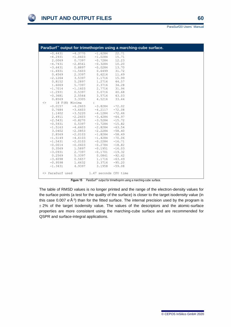
INPUT AND OUTPUT FILES 60
ParaSurf20 Users´ Manual
© CEPOS InSilico GmbH 2020
ParaSurf™ output for trimethoprim using a marching-cube surface.
-0.4431 -4.3770 -1.6284 22.71
-4.2931 -1.0603 -1.0284 15.71
2.0069 0.7397 -0.7284 12.23
-4.7431 -2.8561 -0.3284 10.20
-3.6431 0.8897 -0.0284 13.70
-1.6931 -1.5603 0.6499 31.72
0.4569 2.3397 0.6216 11.69
-2.1264 3.5397 1.1716 15.99
0.8152 5.2897 1.2716 44.57
1.6069 5.7397 2.3716 34.28
-1.7014 -1.1603 2.7716 31.94
-1.2931 0.5397 3.0716 40.68
-0.3681 2.5564 3.5716 43.03
0.8569 3.3305 4.5216 33.44
<> 18 F(N) Minima :
-0.0157 -4.2603 -3.8284 -72.02
0.7684 -3.6603 -4.2117 -72.08
1.1402 -3.5220 -4.1284 -72.46
2.4911 -2.2603 -3.4284 -64.97
-2.5431 -0.8270 -3.5284 -15.72
-0.5931 0.5397 -3.7284 -15.82
-1.5163 -4.6603 -2.8284 -63.54
3.0402 -2.0853 -2.2284 -58.40
2.8569 -2.0103 -1.8284 -58.49
-1.5149 -4.6103 -1.4284 -70.06
-1.5431 -2.0103 -0.2284 -16.71
-0.0014 -0.0603 -0.2784 -18.82
0.3569 1.5897 -0.1951 -16.03
-3.0931 2.7397 -0.1701 -19.32
0.2569 5.3397 0.0841 -92.42
-3.6098 0.5657 1.1716 -63.49
-0.9598 1.6632 3.3716 -95.20
-1.3431 4.9397 3.1958 -59.08
<> ParaSurf used 1.47 seconds CPU time
Figure 15 ParaSurf™ output for trimethoprim using a marching-cube surface.
The table of RMSD values is no longer printed and the range of the electron-density values for
the surface points (a test for the quality of the surface) is closer to the target isodensity value (in
this case 0.007 e-Å-3) than for the fitted surface. The internal precision used by the program is
2% of the target isodensity value. The values of the descriptors and the atomic-surface
properties are more consistent using the marching-cube surface and are recommended for
QSPR and surface-integral applications.
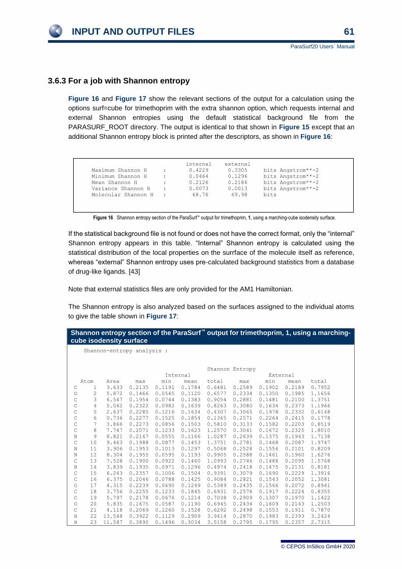
INPUT AND OUTPUT FILES 61
ParaSurf20 Users´ Manual
© CEPOS InSilico GmbH 2020
3.6.3 For a job with Shannon entropy
Figure 16 and Figure 17 show the relevant sections of the output for a calculation using the
options surf=cube for trimethoprim with the extra shannon option, which requests internal and
external Shannon entropies using the default statistical background file from the
PARASURF_ROOT directory. The output is identical to that shown in Figure 15 except that an
additional Shannon entropy block is printed after the descriptors, as shown in Figure 16:
Figure 16 Shannon entropy section of the ParaSurf™ output for trimethoprim, 1, using a marching-cube isodensity surface.
If the statistical background file is not found or does not have the correct format, only the “internal”
Shannon entropy appears in this table. “Internal” Shannon entropy is calculated using the
statistical distribution of the local properties on the surrface of the molecule itself as reference,
whereas “external” Shannon entropy uses pre-calculated background statistics from a database
of drug-like ligands. [43]
Note that external statistics files are only provided for the AM1 Hamiltonian.
The Shannon entropy is also analyzed based on the surfaces assigned to the individual atoms
to give the table shown in Figure 17:
Shannon entropy section of the ParaSurf™ output for trimethoprim, 1, using a marching-cube isodensity surface
Shannon-entropy analysis :
Shannon Entropy
Internal External
Atom Area max min mean total max min mean total
C 1 3.633 0.2135 0.1191 0.1784 0.6481 0.2589 0.1902 0.2189 0.7952
O 2 5.872 0.1466 0.0545 0.1120 0.6577 0.2334 0.1350 0.1985 1.1656
C 3 6.547 0.1954 0.0744 0.1383 0.9054 0.2881 0.1481 0.2100 1.3751
C 4 5.042 0.2322 0.0982 0.1639 0.8263 0.3080 0.1634 0.2373 1.1966
C 5 2.637 0.2285 0.1216 0.1634 0.4307 0.3065 0.1978 0.2332 0.6148
C 6 0.736 0.2277 0.1525 0.1854 0.1365 0.2571 0.2264 0.2415 0.1778
C 7 3.866 0.2273 0.0856 0.1503 0.5810 0.3133 0.1582 0.2203 0.8519
C 8 7.747 0.2071 0.1233 0.1623 1.2570 0.3041 0.1672 0.2325 1.8010
N 9 8.821 0.2147 0.0555 0.1166 1.0287 0.2639 0.1375 0.1943 1.7138
C 10 9.463 0.1988 0.0877 0.1453 1.3751 0.2781 0.1468 0.2087 1.9747
N 11 3.906 0.1953 0.1013 0.1297 0.5068 0.2528 0.1556 0.2101 0.8209
N 12 8.304 0.1955 0.0595 0.1193 0.9905 0.2588 0.1461 0.1960 1.6276
C 13 7.528 0.1900 0.0922 0.1460 1.0993 0.2746 0.1488 0.2095 1.5768
N 14 3.839 0.1935 0.0971 0.1296 0.4974 0.2418 0.1475 0.2131 0.8181
C 15 6.243 0.2357 0.1006 0.1504 0.9391 0.3079 0.1690 0.2229 1.3916
C 16 6.375 0.2046 0.0788 0.1425 0.9084 0.2821 0.1543 0.2052 1.3081
O 17 4.315 0.2239 0.0690 0.1249 0.5389 0.2435 0.1566 0.2072 0.8941
C 18 3.756 0.2255 0.1233 0.1845 0.6931 0.2578 0.1917 0.2224 0.8355
C 19 5.797 0.2178 0.0676 0.1214 0.7038 0.2909 0.1307 0.1970 1.1422
O 20 5.835 0.1675 0.0587 0.1190 0.6945 0.2434 0.1609 0.2143 1.2503
C 21 4.118 0.2069 0.1260 0.1528 0.6292 0.2498 0.1553 0.1911 0.7870
H 22 13.548 0.3922 0.1129 0.2909 3.9414 0.2870 0.1983 0.2393 3.2424
H 23 11.587 0.3890 0.1496 0.3034 3.5158 0.2795 0.1795 0.2357 2.7315
internal external
Maximum Shannon H : 0.4229 0.3305 bits Angstrom**-2
Minimum Shannon H : 0.0464 0.1296 bits Angstrom**-2
Mean Shannon H : 0.2126 0.2186 bits Angstrom**-2
Variance Shannon H : 0.0073 0.0013 bits Angstrom**-2
Molecular Shannon H : 68.76 69.98 bits
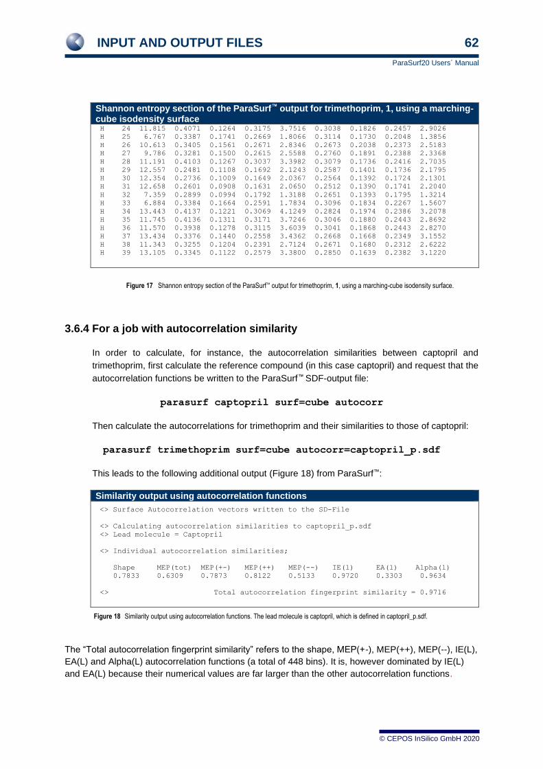
INPUT AND OUTPUT FILES 62
ParaSurf20 Users´ Manual
© CEPOS InSilico GmbH 2020
Shannon entropy section of the ParaSurf™ output for trimethoprim, 1, using a marching-cube isodensity surface H 24 11.815 0.4071 0.1264 0.3175 3.7516 0.3038 0.1826 0.2457 2.9026
H 25 6.767 0.3387 0.1741 0.2669 1.8066 0.3114 0.1730 0.2048 1.3856
H 26 10.613 0.3405 0.1561 0.2671 2.8346 0.2673 0.2038 0.2373 2.5183
H 27 9.786 0.3281 0.1500 0.2615 2.5588 0.2760 0.1891 0.2388 2.3368
H 28 11.191 0.4103 0.1267 0.3037 3.3982 0.3079 0.1736 0.2416 2.7035
H 29 12.557 0.2481 0.1108 0.1692 2.1243 0.2587 0.1401 0.1736 2.1795
H 30 12.354 0.2736 0.1009 0.1649 2.0367 0.2564 0.1392 0.1724 2.1301
H 31 12.658 0.2601 0.0908 0.1631 2.0650 0.2512 0.1390 0.1741 2.2040
H 32 7.359 0.2899 0.0994 0.1792 1.3188 0.2651 0.1393 0.1795 1.3214
H 33 6.884 0.3384 0.1664 0.2591 1.7834 0.3096 0.1834 0.2267 1.5607
H 34 13.443 0.4137 0.1221 0.3069 4.1249 0.2824 0.1974 0.2386 3.2078
H 35 11.745 0.4136 0.1311 0.3171 3.7246 0.3046 0.1880 0.2443 2.8692
H 36 11.570 0.3938 0.1278 0.3115 3.6039 0.3041 0.1868 0.2443 2.8270
H 37 13.434 0.3376 0.1440 0.2558 3.4362 0.2668 0.1668 0.2349 3.1552
H 38 11.343 0.3255 0.1204 0.2391 2.7124 0.2671 0.1680 0.2312 2.6222
H 39 13.105 0.3345 0.1122 0.2579 3.3800 0.2850 0.1639 0.2382 3.1220
Figure 17 Shannon entropy section of the ParaSurf™ output for trimethoprim, 1, using a marching-cube isodensity surface.
3.6.4 For a job with autocorrelation similarity
In order to calculate, for instance, the autocorrelation similarities between captopril and
trimethoprim, first calculate the reference compound (in this case captopril) and request that the
autocorrelation functions be written to the ParaSurf™ SDF-output file:
parasurf captopril surf=cube autocorr
Then calculate the autocorrelations for trimethoprim and their similarities to those of captopril:
parasurf trimethoprim surf=cube autocorr=captopril_p.sdf
This leads to the following additional output (Figure 18) from ParaSurf™:
Similarity output using autocorrelation functions
<> Surface Autocorrelation vectors written to the SD-File
<> Calculating autocorrelation similarities to captopril_p.sdf
<> Lead molecule = Captopril
<> Individual autocorrelation similarities;
Shape MEP(tot) MEP(+-) MEP(++) MEP(--) IE(l) EA(l) Alpha(l)
0.7833 0.6309 0.7873 0.8122 0.5133 0.9720 0.3303 0.9634
<> Total autocorrelation fingerprint similarity = 0.9716
Figure 18 Similarity output using autocorrelation functions. The lead molecule is captopril, which is defined in captopril_p.sdf.
The “Total autocorrelation fingerprint similarity” refers to the shape, MEP(+-), MEP(++), MEP(--), IE(L),
EA(L) and Alpha(L) autocorrelation functions (a total of 448 bins). It is, however dominated by IE(L)
and EA(L) because their numerical values are far larger than the other autocorrelation functions.

INPUT AND OUTPUT FILES 63
ParaSurf20 Users´ Manual
© CEPOS InSilico GmbH 2020
3.7 ParaSurf™ SDF-output
The SDF output file (a fixed-format file) contains additional blocks with the information generated by
ParaSurf™. These are:
<ParaSurf OPTIONS>
The ParaSurf™ OPTIONS block consists of one line giving the options used in the ParaSurf™ calculation.
These are:
<surface> <fit> <electrostatic model> <isodensity level> (a4,2x,a4,2x,a5,2x,f8.3)
Where the individual variables can be:
<surface> WRAP
CUBE
Shrink-wrap surface
Marching-cube surface
<fit> NONE
ISO
SPHH
No fitting, unsmoothed marching-cube surface
Marching-cube surface corrected to 2% of the
preset isodensity value
Spherical-harmonic surface fit
<electrostatic model> NAOPC
MULTI
NAO-PC electrostatics
Multipole electrostatics
<isodensity level> n.nn The target isodensity value in e-Å-3
<solvent probe radius> The radius of the solvent probe used to
calculate the SES or SAS
<triangulation mesh> The mesh size used to triangulate the
Surface
<MOLECULAR_CENTERS>
The molecular centres block appears only for calculations that use spherical harmonic fits. It includes
two lines of the form:
"Spherical harmonic center = ", 3f12.6
"Center of gravity = ", 3f12.6
These blocks give the x, y and z coordinates of the centre of the molecule used for the spherical-
harmonic fit and the centre of gravity, respectively. These two centres are usually identical, but may be
different if the centre of gravity lies outside the molecule (e.g. for U-shaped molecules).
<SPHERICAL_HARMONIC_……>
The spherical harmonic fits are described in <SPHERICAL_HARMONIC_…..> blocks. These blocks
all have the same format and vary only in the property described. Each block has the form:

INPUT AND OUTPUT FILES 64
ParaSurf20 Users´ Manual
© CEPOS InSilico GmbH 2020
Order = nn ("Order = ",i4)
l( )m = -l to l (I5, 10f8.4/5x,10f8.4/5x,10f8.4/5x,10f8.4)
(One set of coefficients each for l = 1 to 15)
RMSDs:
l, RMSD1, RMSD2
(“RMSDs:”)
(i8, 2f12.8)
(One line for each l for l = 1 to 15, where RMSD1 is the area-weighted RMSD and
RMSD2 the simple RMSD)
There are six such blocks, indicated by the tags:
<SPHERICAL_HARMONIC_SURFACE> The fitted molecular surface (radial distances) in Ångstrom
<SPHERICAL_HARMONIC_MEP> The MEP values at the spherical-harmonic surface (l = 20) in kcal mol-1
<SPHERICAL_HARMONIC_IE(l)> The IEL values at the spherical-harmonic surface (l = 20) in kcal mol-1
<SPHERICAL_HARMONIC_EA(l)> The EAL values at the spherical-harmonic surface (l = 20) in kcal mol-1
<SPHERICAL_HARMONIC_ALPHA(l)> The L values at the spherical-harmonic surface (l = 20) in kcal mol-1
<SPHERICAL_HARMONIC_FIELD(N)> The FN values at the spherical-harmonic surface (l = 20) in kcal mol-1 Å-1
<ParaSurf Descriptors>
The ParaSurf™ descriptors block lists the calculated descriptors in the following groups:
Molecular: , D, , MW, G, , VOL
("Molecular ",5f10.4,2f10.2)
MEP: , , , , , , , , , , , , ,
("MEP ",7f10.2/10x, f10.2,5f10.4,2x,g12.6)
IE(l): , , , , , , ,
("IE(l) ",5f10.2,2f10.4/12x,g12.6)
EA(l): , , , , , , , , , , , , ,
,
("EA(l) ",7f10.2/2f10.2,2f10.4,f10.2,2f10.4/12x,g12.6)
Eneg(l): , , , , , , ,
("Eneg(l) ",5f10.2,2f10.4/12x,g12.6)
Hard(l): , , , , , , ,
("Hard(l) ",5f10.2,2f10.4/12x,g12.6)
Alpha(l): , , , , , , ,
("Alpha(l) ",5f10.2,2f10.4/12x,g12.6)
FN , , , , , , , , , , , ,
("Field desc",7f10.4/" ",6f10.4)
Jobs that include Shannon entropy give two extra sets of descriptors:
m
lc
maxV minV V+ V− V V 2 +
2 −
2
Tot 2
tot 1
V 2
V V
max
LIE min
LIE LIE LIE 2
IE 1
IE 2
IE IE
max
LEA min
LEA LEA + LEA − LEA LEA 2
EA +
2
EA −
2
EA EAEA +
EA
+ 1
EA
2
EA EA
max
Lmin
L L L2
1
2
max
Lmin
L L L2
1
2
max
Lmin
L L L2
1
2
max
NF min
NF NF 2
F2
F +
2
F − F 1NF 2
NFNF NF
+NF
−NF

INPUT AND OUTPUT FILES 65
ParaSurf20 Users´ Manual
© CEPOS InSilico GmbH 2020
Shannon(i): , , , ,
("Shannon(i) ",4f10.4,f10.2,f10.4)
Shannon(e): , , , ,
("Shannon(e) ",4f10.4,f10.2,f10.4)
For calculations using a spherical-harmonic fit, the hybridization coefficients are printed to the .sdf file
as follows (tag line followed by as many lines with the coefficients as necessary):
<SHAPE HYBRIDS> (15 coefficients, 6f12.6)
<MEP HYBRIDS> (20 coefficients, 6f12.6
<IE(L) HYBRIDS> (20 coefficients, 6f12.2)
<EA(L) HYBRIDS> (20 coefficients, 6f12.2)
<ALPHA(L) HYBRIDS> (20 coefficients, 6f12.8)
<FIELD(N) HYBRIDS> (20 coefficients, 6f12.4)
The hybridization coefficients are listed in order of increasing i from zero, exactly as in the output file.
The atomic surface properties are listed in the atomic order according to the following headings (tag line
followed by as many lines with the surface properties as necessary):
<ATOMIC SURFACE AREAS> Areas (10f8.4)
<ATOMIC SURFACE MEP MAXIMA> MEP maxima (10f8.2)
<ATOMIC SURFACE MEP MINIMA> MEP minima (10f8.2)
<ATOMIC SURFACE IE(L) MAXIMA> IE(l) maxima (10f8.2)
<ATOMIC SURFACE IE(L) MINIMA> IE(l) minima (10f8.2)
<ATOMIC SURFACE EA(L) MAXIMA> EA(l) maxima (10f8.2)
<ATOMIC SURFACE EA(L) MINIMA> EA(l) minima (10f8.2)
<ATOMIC SURFACE MEAN POL> Mean pol. (10f8.4)
<ATOMIC SURFACE FIELD(N) MAXIMA> FN maxima (10f8.2)
<ATOMIC SURFACE FIELD(N) MINIMA> FN minima (10f8.2)
The properties correspond exactly to those printed in the table of surface properties in the output file.
<PROPERTY MAXIMA and MINIMA>
max
inH min
inH inH 2
inHinH
max
exH min
exH exH 2
exHexH
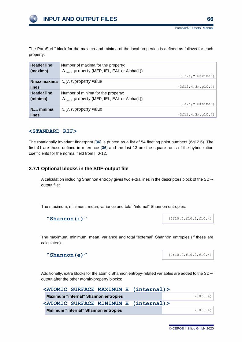
INPUT AND OUTPUT FILES 66
ParaSurf20 Users´ Manual
© CEPOS InSilico GmbH 2020
The ParaSurf™ block for the maxima and minima of the local properties is defined as follows for each
property:
Header line
(maxima)
Number of maxima for the property:
(MEP, IEL, EAL or Alpha(L))
(I3,a," Maxima")
Nmax maxima
lines
(3f12.4,3x,g10.4)
Header line
(minima)
Number of minima for the property:
(MEP, IEL, EAL or Alpha(L))
(I3,a," Minima")
Nmin minima
lines
(3f12.4,3x,g10.4)
<STANDARD RIF>
The rotationally invariant fingerprint [36] is printed as a list of 54 floating point numbers (6g12.6). The
first 41 are those defined in reference [36] and the last 13 are the square roots of the hybridization
coefficients for the normal field from l=0-12.
3.7.1 Optional blocks in the SDF-output file
A calculation including Shannon entropy gives two extra lines in the descriptors block of the SDF-
output file:
The maximum, minimum, mean, variance and total “internal” Shannon entropies.
“Shannon(i)” (4f10.4,f10.2,f10.4)
The maximum, minimum, mean, variance and total “external” Shannon entropies (if these are
calculated).
“Shannon(e)” (4f10.4,f10.2,f10.4)
Additionally, extra blocks for the atomic Shannon entropy-related variables are added to the SDF-
output after the other atomic-property blocks:
<ATOMIC SURFACE MAXIMUM H (internal)>
Maximum “internal” Shannon entropies (10f8.4)
<ATOMIC SURFACE MINIMUM H (internal)>
Minimum “internal” Shannon entropies (10f8.4)
max , propertyN
, , , property valuex y z
max , propertyN
, , , property valuex y z

INPUT AND OUTPUT FILES 67
ParaSurf20 Users´ Manual
© CEPOS InSilico GmbH 2020
<ATOMIC SURFACE MEAN H (internal)>
Mean “internal” Shannon entropies (10f8.4)
<ATOMIC SURFACE TOTAL H (internal)>
Total “internal” Shannon entropies (10f8.4)
If the external Shannon entropy is also calculated, the following blocks are also written:
<ATOMIC SURFACE MAXIMUM H (external)>
Maximum “external” Shannon entropies (10f8.4)
<ATOMIC SURFACE MINIMUM H (external)>
Minimum “external” Shannon entropies (10f8.4)
<ATOMIC SURFACE MEAN H (external)>
Mean “external” Shannon entropies (10f8.4)
<ATOMIC SURFACE TOTAL H (external)>
Total “external” Shannon entropies (10f8.4)
For calculations that include surface autocorrelations, these are written in the following blocks:
<SURFACE AUTOCORRELATION PARAMETERS>
The number of autocorrelation points ("ncorr = ",i6)
The lower end of the autocorrelation range ("rmin = ",f10.6)
The bin size ("dcorr = ",f10.6)
This block then contains a table that gives all the autocorrelations as a table with the following
headings:
Table 7 Column headings and definitions for autocorrelation tables.
Column heading Contents
R Reference distance (R in Equation (18))
shape Shape autocorrelation
MEP(Tot) Total MEP autocorrelation
MEP(+-) MEP +/- autocorrelation
MEP(++) MEP +/+ autocorrelation
MEP(--) MEP -/- autocorrelation
IE(L) IEL autocorrelation
EA(L) EAL autocorrelation
Alpha(L) Alpha(L) autocorrelation
The format of the columns is (f8.2,2x,8g15.6)
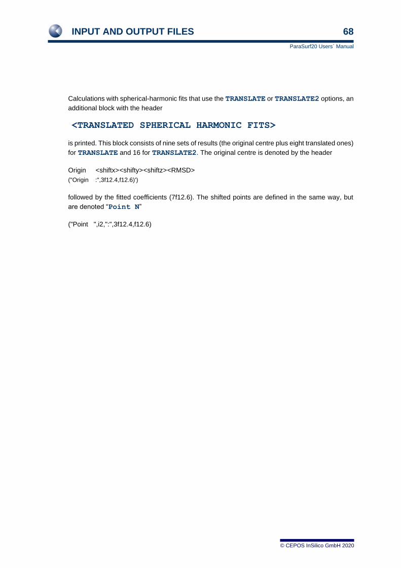
INPUT AND OUTPUT FILES 68
ParaSurf20 Users´ Manual
© CEPOS InSilico GmbH 2020
Calculations with spherical-harmonic fits that use the TRANSLATE or TRANSLATE2 options, an
additional block with the header
<TRANSLATED SPHERICAL HARMONIC FITS>
is printed. This block consists of nine sets of results (the original centre plus eight translated ones)
for TRANSLATE and 16 for TRANSLATE2. The original centre is denoted by the header
Origin <shiftx> <shifty> <shiftz> <RMSD>
("Origin :",3f12.4,f12.6)')
followed by the fitted coefficients (7f12.6). The shifted points are defined in the same way, but
are denoted “Point N”
("Point ",i2,":",3f12.4,f12.6)
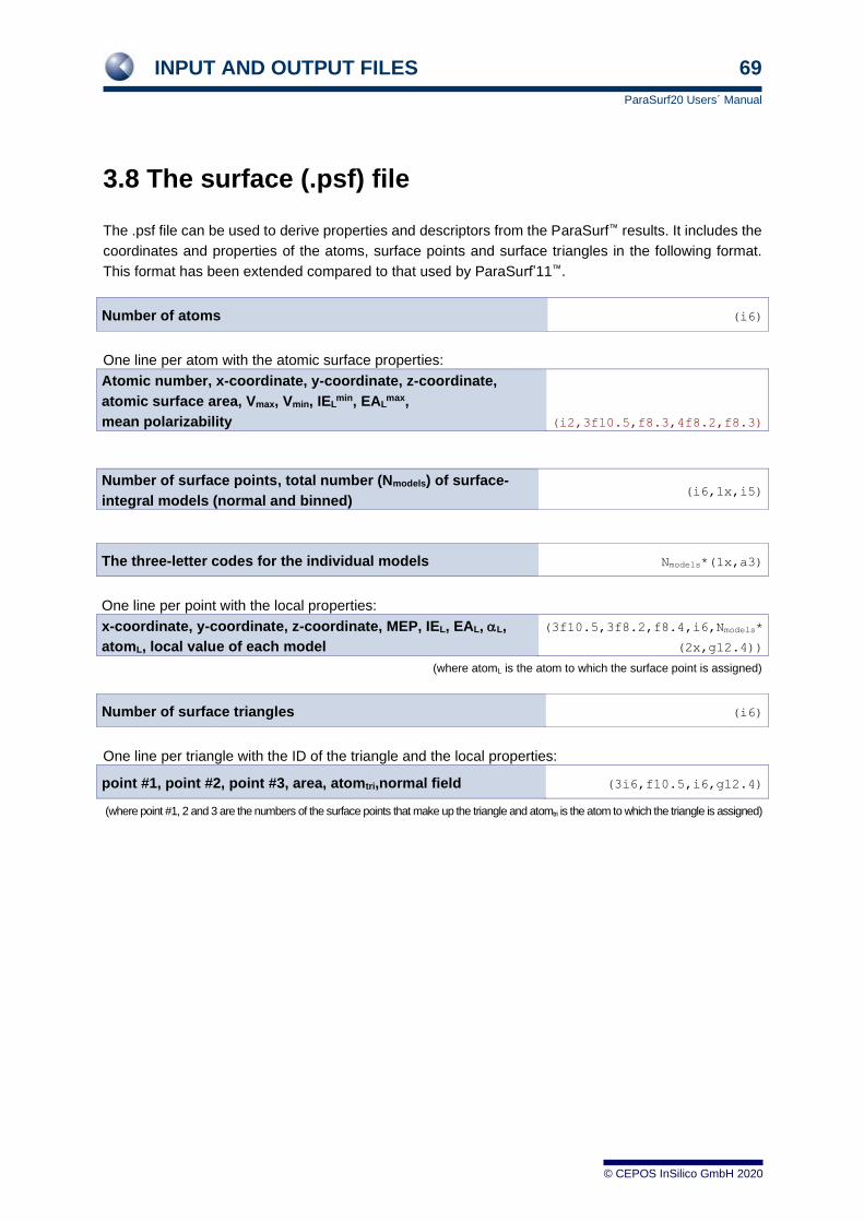
INPUT AND OUTPUT FILES 69
ParaSurf20 Users´ Manual
© CEPOS InSilico GmbH 2020
3.8 The surface (.psf) file
The .psf file can be used to derive properties and descriptors from the ParaSurf™ results. It includes the
coordinates and properties of the atoms, surface points and surface triangles in the following format.
This format has been extended compared to that used by ParaSurf’11™.
Number of atoms (i6)
One line per atom with the atomic surface properties:
Atomic number, x-coordinate, y-coordinate, z-coordinate,
atomic surface area, Vmax, Vmin, IELmin, EAL
max,
mean polarizability (i2,3f10.5,f8.3,4f8.2,f8.3)
Number of surface points, total number (Nmodels) of surface-
integral models (normal and binned) (i6,1x,i5)
The three-letter codes for the individual models Nmodels*(1x,a3)
One line per point with the local properties:
x-coordinate, y-coordinate, z-coordinate, MEP, IEL, EAL, L,
atomL, local value of each model
(3f10.5,3f8.2,f8.4,i6,Nmodels*
(2x,g12.4))
(where atomL is the atom to which the surface point is assigned)
Number of surface triangles (i6)
One line per triangle with the ID of the triangle and the local properties:
point #1, point #2, point #3, area, atomtri,normal field (3i6,f10.5,i6,g12.4)
(where point #1, 2 and 3 are the numbers of the surface points that make up the triangle and atomtri is the atom to which the triangle is assigned)
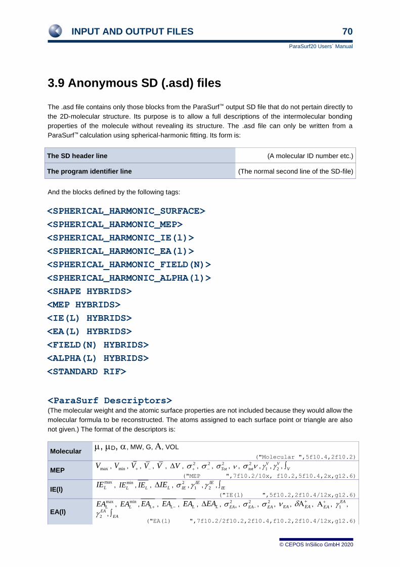
INPUT AND OUTPUT FILES 70
ParaSurf20 Users´ Manual
© CEPOS InSilico GmbH 2020
3.9 Anonymous SD (.asd) files
The .asd file contains only those blocks from the ParaSurf™ output SD file that do not pertain directly to
the 2D-molecular structure. Its purpose is to allow a full descriptions of the intermolecular bonding
properties of the molecule without revealing its structure. The .asd file can only be written from a
ParaSurf™ calculation using spherical-harmonic fitting. Its form is:
The SD header line (A molecular ID number etc.)
The program identifier line (The normal second line of the SD-file)
And the blocks defined by the following tags:
<SPHERICAL_HARMONIC_SURFACE>
<SPHERICAL_HARMONIC_MEP>
<SPHERICAL_HARMONIC_IE(l)>
<SPHERICAL_HARMONIC_EA(l)>
<SPHERICAL_HARMONIC_FIELD(N)>
<SPHERICAL_HARMONIC_ALPHA(l)>
<SHAPE HYBRIDS>
<MEP HYBRIDS>
<IE(L) HYBRIDS>
<EA(L) HYBRIDS>
<FIELD(N) HYBRIDS>
<ALPHA(L) HYBRIDS>
<STANDARD RIF>
<ParaSurf Descriptors> (The molecular weight and the atomic surface properties are not included because they would allow the
molecular formula to be reconstructed. The atoms assigned to each surface point or triangle are also
not given.) The format of the descriptors is:
Molecular , D, , MW, G, , VOL
("Molecular ",5f10.4,2f10.2)
MEP , , , , , , , , , , , , ,
("MEP ",7f10.2/10x, f10.2,5f10.4,2x,g12.6)
IE(l) , , , , , , ,
("IE(l) ",5f10.2,2f10.4/12x,g12.6)
EA(l) , , , , , , , , , , , , ,
, ("EA(l) ",7f10.2/2f10.2,2f10.4,f10.2,2f10.4/12x,g12.6)
maxV minV V+ V− V V 2 +
2 −
2
Tot 2
tot 1
V 2
V V
max
LIE min
LIE LIE LIE 2
IE 1
IE 2
IE IE
max
LEA min
LEA LEA + LEA − LEA LEA 2
EA +
2
EA −
2
EA EA EA +EA
+ 1
EA
2
EA EA
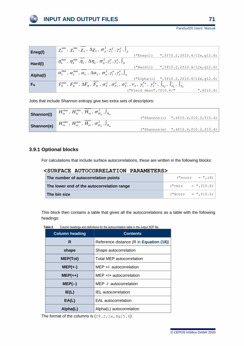
INPUT AND OUTPUT FILES 71
ParaSurf20 Users´ Manual
© CEPOS InSilico GmbH 2020
Eneg(l) , , , , , , ,
("Eneg(l) ",5f10.2,2f10.4/12x,g12.6)
Hard(l) , , , , , , ,
("Hard(l) ",5f10.2,2f10.4/12x,g12.6)
Alpha(l) , , , , , , ,
("Alpha(l) ",5f10.2,2f10.4/12x,g12.6)
FN , , , , , , , , , , , ,
("Field desc",7f10.4/" ",6f10.4)
Jobs that include Shannon entropy give two extra sets of descriptors:
Shannon(i) , , , ,
("Shannon(i) ",4f10.4,f10.2,f10.4)
Shannon(e) , , , ,
("Shannon(e) ",4f10.4,f10.2,f10.4)
3.9.1 Optional blocks
For calculations that include surface autocorrelations, these are written in the following blocks:
<SURFACE AUTOCORRELATION PARAMETERS>
The number of autocorrelation points ("ncorr = ",i6)
The lower end of the autocorrelation range ("rmin = ",f10.6)
The bin size ("dcorr = ",f10.6)
This block then contains a table that gives all the autocorrelations as a table with the following
headings:
Table 8 Column headings and definitions for the autocorrelation table in the output SDF file.
Column heading Contents
R Reference distance (R in Equation (18))
shape Shape autocorrelation
MEP(Tot) Total MEP autocorrelation
MEP(+-) MEP +/- autocorrelation
MEP(++) MEP +/+ autocorrelation
MEP(--) MEP -/- autocorrelation
IE(L) IEL autocorrelation
EA(L) EAL autocorrelation
Alpha(L) Alpha(L) autocorrelation
The format of the columns is (f8.2,2x,8g15.6)
max
Lmin
L L L2
1
2
max
Lmin
L L L2
1
2
max
Lmin
L L L2
1
2
max
NF min
NF NFNF 2
F2
F +
2
F − F 1NF 2
NFNF NF
+NF
−
max
inH min
inH inH 2
inHinH
max
exH min
exH exH 2
exHexH

INPUT AND OUTPUT FILES 72
ParaSurf20 Users´ Manual
© CEPOS InSilico GmbH 2020
3.10 Grid calculations with ParaSurf™
3.10.1 User-specified Grid
The command
parasurf <filename> estat=multi grid=grid.dat
instructs ParaSurf™ to read a set of Cartesian coordinates from the file grid.dat and to calculate
the log10 of the electron density, the four local properties, the electric field and the derivatives of
the local properties (log(), MEP (=V), IE(l), EA(l) Pol(l), Eneg(l), Hard(l), dV/dx, dV/dy, dV/dz,
d/dx, d/dy, d/dz, dlog()/dx, dlog()/dy, dlog()/dz, dIE(l)/dx, dIE(l)/dy, dIE(l)/dz, dEA(l)/dx,
dEA(l)/dy, dEA(l)/dz, dEneg/dx, dEneg/dy, dEneg/dz, dHard/dx, dHard/dy, dHard/dz). The format
of the file grid.dat (which must be in the same directory as the input) is one line per point
containing the x, y and z coordinates in free format, comma-separated, maximum line length 80
with no trailing comma. For instance, the following grid file (Figure 19):
Figure 19 Sample grid file
gives the output shown in Figure 20.
Sample grid output file (original)
<> ParaSurf'20
<> Copyright (c) 2006-2019 Cepos InSilico GmbH All rights reserved.
<> Input = trimethoprim.sdf
<<>> Molecule 1 of 1 <<>>
<> Program options :
Calculating local properties using grid file grid.txt
Using multipole electrostatics
<> AM1 calculation for Trimethoprim
x y z log(rho) MEP IE(l) EA(l) Pol(l) Eneg(l) Hard(l) dv/dx dv/dy dv/dz dRho/dx dRho/dy dRho/dz dlogR/dx dlogR/dy dlogR/dz dIEl/dx dIEl/dy dIEl/dz dEAl/dx dEAl/dy dEAl/dz dEneg/dx dEneg/dy dEneg/dz dHard/dx dHard/dy dHard/dz
-8.01100 -13.72910 -7.91090 -21.981311 -0.14 397.68 -93.93 0.4314 151.87 245.80 6.165E-02 -3.937E-04 -3.356E-02 1.787E-22 3.681E-22 2.289E-22 7.432E-01 1.531E+00 9.523E-01 -1.928E+00 2.328E+00 -2.815E+00 4.315E-02 -5.509E-02 6.822E-02 -9.423E-01 1.137E+00 -1.374E+00 -9.855E-01 1.192E+00 -1.442E+00
-8.01100 -13.72910 -6.91090 -21.096656 -0.10 395.21 -93.87 0.4454 150.67 244.54 6.241E-02 -9.348E-03 -4.102E-02 1.426E-21 2.938E-21 1.501E-21 7.739E-01 1.594E+00 8.142E-01 -1.870E+00 1.701E+00 -2.117E+00 4.256E-02 -4.129E-02 5.351E-02 -9.135E-01 8.301E-01 -1.032E+00 -9.561E-01 8.714E-01 -1.085E+00
-8.01100 -13.72910 -5.91090 -20.358433 -0.05 393.44 -93.82 0.4572 149.81 243.63 6.127E-02 -2.024E-02 -4.705E-02 8.086E-21 1.666E-20 6.653E-21 8.016E-01 1.651E+00 6.595E-01 -1.826E+00 1.224E+00 -1.434E+00 4.188E-02 -3.019E-02 3.833E-02 -8.922E-01 5.971E-01 -6.979E-01 -9.341E-01 6.273E-01 -7.362E-01
-8.01100 -13.72910 -4.91090 -19.782872 -0.01 392.34 -93.79 0.4658 149.27 243.07 5.815E-02 -3.235E-02 -5.068E-02 3.130E-20 6.447E-20 1.857E-20 8.245E-01 1.698E+00 4.892E-01 -1.809E+00 8.945E-01 -7.602E-01 4.140E-02 -2.211E-02 2.297E-02 -8.840E-01 4.362E-01 -3.686E-01 -9.254E-01 4.583E-01 -3.916E-01
-8.01100 -13.72910 -3.91090 -19.384276 0.05 391.92 -93.78 0.4701 149.07 242.85 5.324E-02 -4.454E-02 -5.122E-02 7.995E-20 1.647E-19 2.910E-20 8.412E-01 1.733E+00 3.061E-01 -1.830E+00 7.083E-01 -6.999E-02 4.138E-02 -1.717E-02 7.305E-03 -8.942E-01 3.456E-01 -3.134E-02 -9.356E-01 3.628E-01 -3.865E-02
-8.01100 -13.72910 -2.91090 -19.173520 0.10 392.22 -93.78 0.4694 149.22 243.00 4.695E-02 -5.549E-02 -4.847E-02 1.313E-19 2.705E-19 1.766E-20 8.503E-01 1.751E+00 1.143E-01 -1.896E+00 6.709E-01 6.788E-01 4.197E-02 -1.549E-02 -9.132E-03 -9.269E-01 3.277E-01 3.348E-01 -9.688E-01 3.432E-01 3.439E-01
-8.01100 -13.72910 -1.91090 -19.156717 0.14 393.32 -93.80 0.4634 149.76 243.56 3.983E-02 -6.402E-02 -4.281E-02 1.366E-19 2.814E-19 -1.297E-20 8.511E-01 1.753E+00 -8.082E-02 -2.012E+00 8.029E-01 1.542E+00 4.320E-02 -1.731E-02 -2.699E-02 -9.846E-01 3.928E-01 7.576E-01 -1.028E+00 4.101E-01 7.846E-01
-8.01100 -13.72910 -0.91090 -19.334354 0.18 395.36 -93.83 0.4522 150.76 244.60 3.246E-02 -6.935E-02 -3.510E-02 8.993E-20 1.852E-19 -2.917E-20 8.434E-01 1.737E+00 -2.736E-01 -2.180E+00 1.147E+00 2.583E+00 4.486E-02 -2.306E-02 -4.672E-02 -1.068E+00 5.618E-01 1.268E+00 -1.112E+00 5.849E-01 1.315E+00
-8.01100 -13.72910 0.08910 -19.701160 0.21 398.56 -93.89 0.4368 152.33 246.23 2.530E-02 -7.131E-02 -2.641E-02 3.793E-20 7.814E-20 -2.100E-20 8.279E-01 1.705E+00 -4.583E-01 -2.390E+00 1.765E+00 3.857E+00 4.646E-02 -3.306E-02 -6.811E-02 -1.172E+00 8.659E-01 1.895E+00 -1.218E+00 8.989E-01 1.963E+00
-8.01100 -13.72910 1.08910 -20.246709 0.23 403.16 -93.97 0.4182 154.60 248.57 1.868E-02 -7.022E-02 -1.770E-02 1.051E-20 2.166E-20 -8.224E-21 8.058E-01 1.660E+00 -6.304E-01 -2.622E+00 2.727E+00 5.387E+00 4.723E-02 -4.701E-02 -8.951E-02 -1.287E+00 1.340E+00 2.649E+00 -1.335E+00 1.387E+00 2.738E+00
<> ParaSurf used 0.15 seconds CPU time
Sample grid output file (.txt)
<> ParaSurf'20
<> Copyright (c) 2006-2020 Cepos InSilico GmbH. All rights reserved.
<> Input = trimethoprim.sdf
<<>> Molecule 1 of 1 <<>>
<> Program options :
-8.01100 , -13.72910 , -7.91090
-8.01100 , -13.72910 , -6.91090
-8.01100 , -13.72910 , -5.91090
-8.01100 , -13.72910 , -4.91090
-8.01100 , -13.72910 , -3.91090
-8.01100 , -13.72910 , -2.91090
-8.01100 , -13.72910 , -1.91090
-8.01100 , -13.72910 , -0.91090
-8.01100 , -13.72910 , 0.08910
-8.01100 , -13.72910 , 1.08910

INPUT AND OUTPUT FILES 73
ParaSurf20 Users´ Manual
© CEPOS InSilico GmbH 2020
Calculating local properties using grid file grid.txt
Using multipole electrostatics
<> AM1 calculation for Trimethoprim
x y z log(rho) MEP IE(l) EA(l) Pol(l) Eneg(l) Hard(l) dv/dx
dv/dy dv/dz dRho/dx dRho/dy dRho/dz dlogR/dx dlogR/dy dlogR/dz dIEl/dx dIEl/dy dIEl/dz
dEAl/dx dEAl/dy dEAl/dz dEneg/dx dEneg/dy dEneg/dz dHard/dx dHard/dy dHard/dz
-8.01100 -13.72910 -7.91090 -21.981311 -0.14 397.68 -93.93 0.4314 151.87 245.80 6.165E-02 -
3.937E-04 -3.356E-02 1.787E-22 3.681E-22 2.289E-22 7.432E-01 1.531E+00 9.523E-01 -1.928E+00 2.328E+00 -
2.815E+00 4.315E-02 -5.509E-02 6.822E-02 -9.423E-01 1.137E+00 -1.374E+00 -9.855E-01 1.192E+00 -1.442E+00
-8.01100 -13.72910 -6.91090 -21.096656 -0.10 395.21 -93.87 0.4454 150.67 244.54 6.241E-02 -
9.348E-03 -4.102E-02 1.426E-21 2.938E-21 1.501E-21 7.739E-01 1.594E+00 8.142E-01 -1.870E+00 1.701E+00 -
2.117E+00 4.256E-02 -4.129E-02 5.351E-02 -9.135E-01 8.301E-01 -1.032E+00 -9.561E-01 8.714E-01 -1.085E+00
-8.01100 -13.72910 -5.91090 -20.358433 -0.05 393.44 -93.82 0.4572 149.81 243.63 6.127E-02 -
2.024E-02 -4.705E-02 8.086E-21 1.666E-20 6.653E-21 8.016E-01 1.651E+00 6.595E-01 -1.826E+00 1.224E+00 -
1.434E+00 4.188E-02 -3.019E-02 3.833E-02 -8.922E-01 5.971E-01 -6.979E-01 -9.341E-01 6.273E-01 -7.362E-01
-8.01100 -13.72910 -4.91090 -19.782872 -0.01 392.34 -93.79 0.4658 149.27 243.07 5.815E-02 -
3.235E-02 -5.068E-02 3.130E-20 6.447E-20 1.857E-20 8.245E-01 1.698E+00 4.892E-01 -1.809E+00 8.945E-01 -7.602E-
01 4.140E-02 -2.211E-02 2.297E-02 -8.840E-01 4.362E-01 -3.686E-01 -9.254E-01 4.583E-01 -3.916E-01
-8.01100 -13.72910 -3.91090 -19.384276 0.05 391.92 -93.78 0.4701 149.07 242.85 5.324E-02 -
4.454E-02 -5.122E-02 7.995E-20 1.647E-19 2.910E-20 8.412E-01 1.733E+00 3.061E-01 -1.830E+00 7.083E-01 -6.999E-
02 4.138E-02 -1.717E-02 7.305E-03 -8.942E-01 3.456E-01 -3.134E-02 -9.356E-01 3.628E-01 -3.865E-02
-8.01100 -13.72910 -2.91090 -19.173520 0.10 392.22 -93.78 0.4694 149.22 243.00 4.695E-02 -
5.549E-02 -4.847E-02 1.313E-19 2.705E-19 1.766E-20 8.503E-01 1.751E+00 1.143E-01 -1.896E+00 6.709E-01 6.788E-
01 4.197E-02 -1.549E-02 -9.132E-03 -9.269E-01 3.277E-01 3.348E-01 -9.688E-01 3.432E-01 3.439E-01
-8.01100 -13.72910 -1.91090 -19.156717 0.14 393.32 -93.80 0.4634 149.76 243.56 3.983E-02 -
6.402E-02 -4.281E-02 1.366E-19 2.814E-19 -1.297E-20 8.511E-01 1.753E+00 -8.082E-02 -2.012E+00 8.029E-01 1.542E+00
4.320E-02 -1.731E-02 -2.699E-02 -9.846E-01 3.928E-01 7.576E-01 -1.028E+00 4.101E-01 7.846E-01
-8.01100 -13.72910 -0.91090 -19.334354 0.18 395.36 -93.83 0.4522 150.76 244.60 3.246E-02 -
6.935E-02 -3.510E-02 8.993E-20 1.852E-19 -2.917E-20 8.434E-01 1.737E+00 -2.736E-01 -2.180E+00 1.147E+00 2.583E+00
4.486E-02 -2.306E-02 -4.672E-02 -1.068E+00 5.618E-01 1.268E+00 -1.112E+00 5.849E-01 1.315E+00
-8.01100 -13.72910 0.08910 -19.701160 0.21 398.56 -93.89 0.4368 152.33 246.23 2.530E-02 -
7.131E-02 -2.641E-02 3.793E-20 7.814E-20 -2.100E-20 8.279E-01 1.705E+00 -4.583E-01 -2.390E+00 1.765E+00 3.857E+00
4.646E-02 -3.306E-02 -6.811E-02 -1.172E+00 8.659E-01 1.895E+00 -1.218E+00 8.989E-01 1.963E+00
-8.01100 -13.72910 1.08910 -20.246709 0.23 403.16 -93.97 0.4182 154.60 248.57 1.868E-02 -
7.022E-02 -1.770E-02 1.051E-20 2.166E-20 -8.224E-21 8.058E-01 1.660E+00 -6.304E-01 -2.622E+00 2.727E+00 5.387E+00
4.723E-02 -4.701E-02 -8.951E-02 -1.287E+00 1.340E+00 2.649E+00 -1.335E+00 1.387E+00 2.738E+00
<> ParaSurf used 0.15 seconds CPU time
Figure 20 Sample grid output file
The name and the extension (if any) of the grid file are free. Only the output file is written. The
units of the local properties are those used in the normal output (i.e. V, IEL, and EAL in kcal mol‑1,
L in Ångstrom3.
3.10.2 Automatic grids
ParaSurf™ can generate grids automatically for lead compounds in CoMFA®-like procedures. The
grid=auto option generates a grid around the molecule (with a 0.5 Å margin around the
positions of the atoms in each direction) and includes all points for which the electron density is
lower than 10-2 (i.e. for points outside the molecule). The spacing of the grid is set to a default
value of 1.0 Å, but can be set to any value up to a maximum of 2.0 Å by the command-line
argument lattice=n.n, which sets the lattice spacing to n.n Å. The grid thus generated is
output (with the values of the local properties analogously to a calculation that uses a predefined
grid and can be used for other molecules that have been aligned with the lead. An additional
output file named <filename>_p.grid. There are two further variations of the automatic grid-
generation procedure: grid=auto excludes any points that are within 0.5 Å of a nucleus,
whereas grid=vdw excludes all grid points within the van der Waals volume of the molecule
and grid=box calculates all points regardless of their proximity to a nucleus.

INPUT AND OUTPUT FILES 74
ParaSurf20 Users´ Manual
© CEPOS InSilico GmbH 2020
3.11 The SIM file format
SIM files must reside in the ParaSurf™ executable directory and are strictly fixed format. SIM files must
be called <filename>.sim, where <filename> must have exactly three characters. A sample
SIM file for a single model (the free energy of solvation in octanol) is shown in Figure 21:
Figure 21 Sample surface-integral model (SIM) file.
The first line, the OPTIONS tag, is compulsory and takes the form:
<OPTIONS>
The second to fifth lines, also compulsory in the order shown above, give the ParaSurf™ options to be
used for the surface-integral model. These options are given in lower case and override conflicting
command-line options.
Line 6 must be the MODELS tag with the format
<MODELS>
Line 7 contains the two integers (Nmodels and Maxterms) that define the number of models given
in the file and the maximum number of terms for any one model. The format is:
Nmodels Maxterms (2i4)
The remainder of the SIM file consists of Nmodels blocks, each of which defines a single model and
has the following format:
Model identifier tag
<MOD> where MOD is a three-letter unique identifier for the model.
Nterms (the number of terms in the model), constant (the constant in the
regression equation) (i4,g12.6)
Model name (for output, maximum 20 characters) (a20)
> <OPTIONS>
surf=cube
fit=isod
estat=multi
iso=0.05
> <MODELS>
1 3
> <DGO>
3 1.61058
DeltaG(n-Octanol)
kcal/mol
-0.01107 F 1.0 0.0 0.0 1.0 0.0 1.0
1.6793d-9 F 1.0 0.0 3.0 0.0 0.0 1.0
-2.0407d-10 T 1.0 0.0 1.0 0.0 1.0 1.5
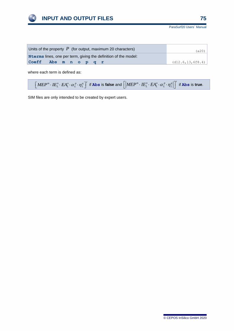
INPUT AND OUTPUT FILES 75
ParaSurf20 Users´ Manual
© CEPOS InSilico GmbH 2020
Units of the property (for output, maximum 20 characters) (a20)
Nterms lines, one per term, giving the definition of the model:
Coeff Abs m n o p q r (d12.6,l3,6f8.4)
where each term is defined as:
if Abs is false and if Abs is true.
SIM files are only intended to be created by expert users.
P
rm n o p q
L L L LMEP IE EA
rm n o p q
L L L LMEP IE EA
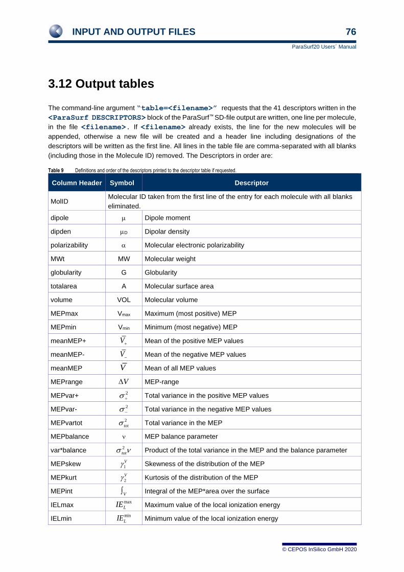
INPUT AND OUTPUT FILES 76
ParaSurf20 Users´ Manual
© CEPOS InSilico GmbH 2020
3.12 Output tables
The command-line argument “table=<filename>” requests that the 41 descriptors written in the
<ParaSurf DESCRIPTORS> block of the ParaSurf™ SD-file output are written, one line per molecule,
in the file <filename>. If <filename> already exists, the line for the new molecules will be
appended, otherwise a new file will be created and a header line including designations of the
descriptors will be written as the first line. All lines in the table file are comma-separated with all blanks
(including those in the Molecule ID) removed. The Descriptors in order are:
Table 9 Definitions and order of the descriptors printed to the descriptor table if requested.
Column Header Symbola Descriptor
MolID Molecular ID taken from the first line of the entry for each molecule with all blanks
eliminated.
dipole Dipole moment
dipden D Dipolar density
polarizability Molecular electronic polarizability
MWt MW Molecular weight
globularity G Globularity
totalarea A Molecular surface area
volume VOL Molecular volume
MEPmax Vmax Maximum (most positive) MEP
MEPmin Vmin Minimum (most negative) MEP
meanMEP+ Mean of the positive MEP values
meanMEP- Mean of the negative MEP values
meanMEP Mean of all MEP values
MEPrange MEP-range
MEPvar+ Total variance in the positive MEP values
MEPvar- Total variance in the negative MEP values
MEPvartot Total variance in the MEP
MEPbalance MEP balance parameter
var*balance Product of the total variance in the MEP and the balance parameter
MEPskew Skewness of the distribution of the MEP
MEPkurt Kurtosis of the distribution of the MEP
MEPint Integral of the MEP*area over the surface
IELmax Maximum value of the local ionization energy
IELmin Minimum value of the local ionization energy
V+
V−
V
V
2 +
2 −
2
tot
2
tot
1
V
2
V
V
max
LIE
min
LIE

INPUT AND OUTPUT FILES 77
ParaSurf20 Users´ Manual
© CEPOS InSilico GmbH 2020
Column Header Symbola Descriptor
IELbar Mean value of the local ionization energy
IELrange Range of the local ionization energy
IELvar Variance in the local ionization energy
IELskew Skewness of the distribution of IE(L)
IELkurt Kurtosis of the distribution of IE(L)
IELint Integral of the IE(L)*area over the surface
EALmax Maximum of the local electron affinity
EALmin Minimum of the local electron affinity
EALbar+ Mean of the positive values of the local electron affinity
EALbar- Mean of the negative values of the local electron affinity
EALbar Mean value of the local electron affinity
EALrange Range of the local electron affinity
EALvar+ Variance in the local electron affinity for all positive values
EALvar- Variance in the local electron affinity for all negative values
EALvartot Sum of the positive and negative variances in the local electron affinity
EALbalance Local electron affinity balance parameter
EALfraction+ Fraction of the surface area with positive local electron affinity
EALarea+ Surface area with positive local electron affinity
EALskew Skewness of the distribution of the MEP
EALkurt Kurtosis of the distribution of the MEP
EALint Integral of the MEP*area over the surface
POLmax Maximum value of the local polarizability
POLmin Minimum value of the local polarizability
POLbar Mean value of the local polarizability
POLrange Range of the local polarizability
POLvar Variance in the local polarizability
POLskew Skewness of the distribution of the local polarizability
POLkurt Kurtosis of the distribution of the local polarizability
POLint Integral of the (L)*area over the surface
ENEGmax Maximum of the local electronegativity
ENEGmin Minimum of the local electronegativity
ENEGbar Mean value of the local electronegativity
LIE
LIE
2
IE
1
IE
2
IE
IE
max
LEA
min
LEA
LEA +
LEA −
LEA
LEA
2
EA +
2
EA −
2
EAtot
EA
EA +
EA
+
1
EA
2
EA
EA
max
L
min
L
L
L
2
1
2
max
L
min
L
L
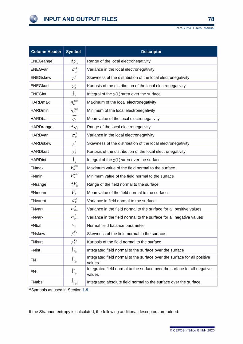
INPUT AND OUTPUT FILES 78
ParaSurf20 Users´ Manual
© CEPOS InSilico GmbH 2020
Column Header Symbola Descriptor
ENEGrange Range of the local electronegativity
ENEGvar Variance in the local electronegativity
ENEGskew Skewness of the distribution of the local electronegativity
ENEGkurt Kurtosis of the distribution of the local electronegativity
ENEGint Integral of the (L)*area over the surface
HARDmax Maximum of the local electronegativity
HARDmin Minimum of the local electronegativity
HARDbar Mean value of the local electronegativity
HARDrange Range of the local electronegativity
HARDvar Variance in the local electronegativity
HARDskew Skewness of the distribution of the local electronegativity
HARDkurt Kurtosis of the distribution of the local electronegativity
HARDint Integral of the (L)*area over the surface
FNmax Maximum value of the field normal to the surface
FNmin Minimum value of the field normal to the surface
FNrange Range of the field normal to the surface
FNmean Mean value of the field normal to the surface
FNvartot Variance in field normal to the surface
FNvar+ Variance in the field normal to the surface for all positive values
FNvar- Variance in the field normal to the surface for all negative values
FNbal Normal field balance parameter
FNskew Skewness of the field normal to the surface
FNkurt Kurtosis of the field normal to the surface
FNint Integrated field normal to the surface over the surface
FN+ Integrated field normal to the surface over the surface for all positive
values
FN- Integrated field normal to the surface over the surface for all negative
values
FNabs Integrated absolute field normal to the surface over the surface
aSymbols as used in Section 1.9.
If the Shannon entropy is calculated, the following additional descriptors are added:
L
2
1
2
max
L
min
L
L
L
2
1
2
max
NF
min
NF
NF
NF
2
F
2
F +
2
F −
F
1NF
2NF
NF
NF
+
NF
−
NF
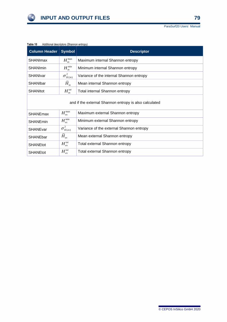
INPUT AND OUTPUT FILES 79
ParaSurf20 Users´ Manual
© CEPOS InSilico GmbH 2020
Table 10 Additional descriptors (Shannon entropy)
Column Header Symbol Descriptor
SHANImax Maximum internal Shannon entropy
SHANImin Minimum internal Shannon entropy
SHANIvar Variance of the internal Shannon entropy
SHANIbar Mean internal Shannon entropy
SHANItot Total internal Shannon entropy
and if the external Shannon entropy is also calculated
SHANEmax Maximum external Shannon entropy
SHANEmin Minimum external Shannon entropy
SHANEvar Variance of the external Shannon entropy
SHANEbar Mean external Shannon entropy
SHANEtot Total external Shannon entropy
SHANEtot Total external Shannon entropy
max
inH
min
inH
2
( )H in
inH
tot
inH
max
exH
min
exH
2
( )H ex
exH
tot
exH
tot
exH
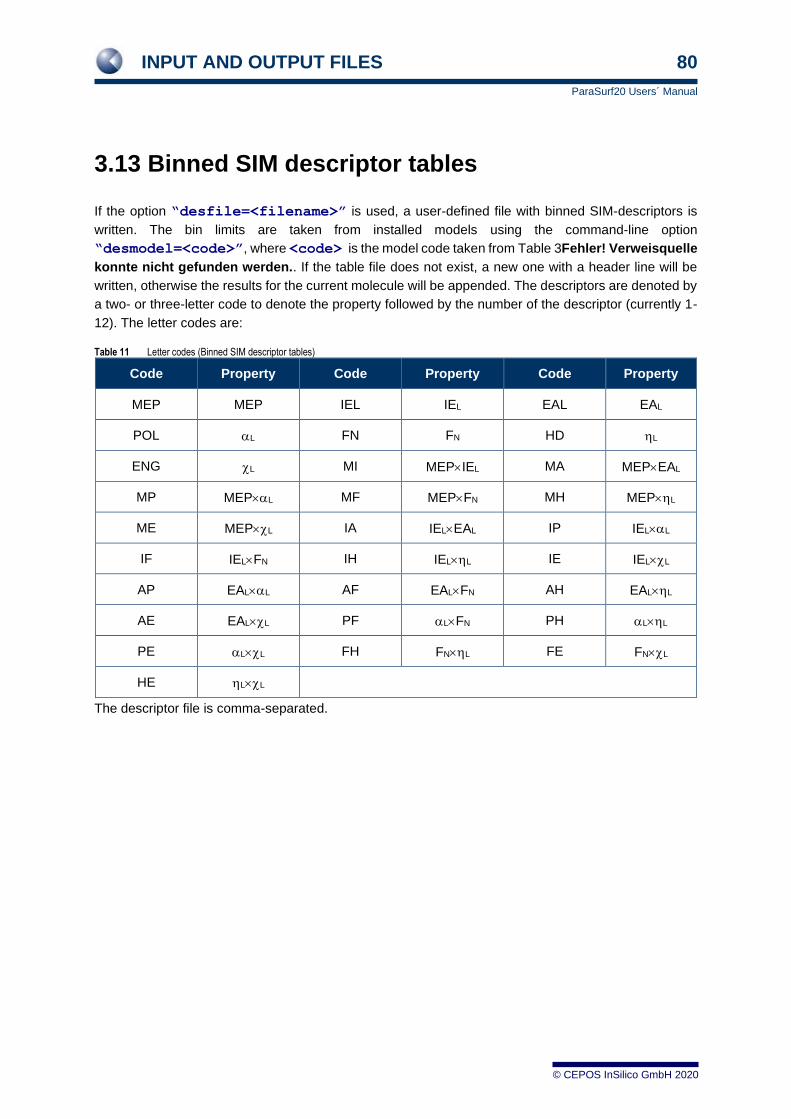
INPUT AND OUTPUT FILES 80
ParaSurf20 Users´ Manual
© CEPOS InSilico GmbH 2020
3.13 Binned SIM descriptor tables
If the option “desfile=<filename>” is used, a user-defined file with binned SIM-descriptors is
written. The bin limits are taken from installed models using the command-line option
“desmodel=<code>”, where <code> is the model code taken from Table 3Fehler! Verweisquelle
konnte nicht gefunden werden.. If the table file does not exist, a new one with a header line will be
written, otherwise the results for the current molecule will be appended. The descriptors are denoted by
a two- or three-letter code to denote the property followed by the number of the descriptor (currently 1-
12). The letter codes are:
Table 11 Letter codes (Binned SIM descriptor tables)
Code Property Code Property Code Property
MEP MEP IEL IEL EAL EAL
POL L FN FN HD L
ENG L MI MEPIEL MA MEPEAL
MP MEPL MF MEPFN MH MEPL
ME MEPL IA IELEAL IP IELL
IF IELFN IH IELL IE IELL
AP EALL AF EALFN AH EALL
AE EALL PF LFN PH LL
PE LL FH FNL FE FNL
HE LL
The descriptor file is comma-separated.

INPUT AND OUTPUT FILES 81
ParaSurf20 Users´ Manual
© CEPOS InSilico GmbH 2020
3.14 Autocorrelation fingerprint and similarity tables
If the option “aclist=<filename>” is used, a user-defined file with the autocorrelation fingerprint
is written. If this file does not exist, it is created and the header line written, otherwise entries are
appended. The ASCII file is comma-separated and contains the molecular identifier followed by 448
binned autocorrelation values in the order Shape, MEP(+-), MEP(++), MEP(--), IE(L), EA(L), Alpha(L)
(64 bins each).
The option “aclist=<filename>” requests a user-defined file with the autocorrelation similarities
to the lead compound defined using the “autocorr = <filename>” keyword. If this file does
not exist, it is created and the header line written, otherwise entries are appended. The ASCII file is has
a fixed format. The header line is
Molid Shape MEP(tot) MEP(+-) MEP(++) MEP(--) IE(l)
EA(l) Alpha(l) Fingerprint
and the similarities are written in format (a20,9f10.4). If the molecular identifier is longer than 20
characters, it will be truncated. The “Fingerprint” similarity considers all 448 autocorrelation values (but
see Section 0.
3.15 Shared files
The Vhamil.par and SIM files are accessed in shared, read-only mode so that multiple ParaSurf™ jobs
can access the same files.
TIPS FOR USING PARASURF19™ 82
ParaSurf20 Users´ Manual
© CEPOS InSilico GmbH 2020
4 TIPS FOR USING PARASURF20™
4.1 Choice of surface
ParaSurf™ was originally written to use isodensity surfaces. However, calculations that use a solvent-
excluded surface are very much faster than their equivalents with isodensity surfaces and will usually
give comparable results. Surface-integral models may benefit from using a solvent-excluded surface
with a solvent radius of 0.5-1.0 Å as this appears to be the most relevant surface for many physical
properties. Surfaces fitted to spherical-harmonic expansions require more CPU-time than marching-
cube surfaces but are essential for fast numerical applications such as ParaFit™. Again, solvent-
excluded shrink-wrap surfaces are faster to calculate than their isodensity equivalents.
4.2 Local properties
The improved local properties implemented in ParaSurf’12™ generally give better QSAR and QSPR
models than the earlier ones available up to ParaSurf’11™. It is therefore recommended that new
projects use the ParaSurf’12™ local properties.
4.3 QSAR using grids
As outlined in Section 3.10.2, ParaSurf™ can generate a grid for the lead molecule automatically that
can then be used for a set of aligned (e.g. with ParaFit™) molecules for grid-based QSAR. This
procedure has proven to be especially effective for test datasets, especially if the molecules are aligned
to a common scaffold, as outlined in Section 1.1
The automatic grid generated for a lead molecule is now written to the file <filename>_p.grid for
use with the remainder of the dataset.

SUPPORT 83
ParaSurf20 Users´ Manual
© CEPOS InSilico GmbH 2020
5 SUPPORT
5.1 Contact
Questions regarding ParaSurf™ should be sent directly to:
5.2 Error reporting
Some of the routines in ParaSurf™ may detect error conditions that have not yet been encountered in
our tests. In this case, an error message will be printed requesting that the input and output files be sent
to the programming team at the above e-mail address. We realize that this will not always be possible
for confidentiality reasons, but if the details can be sent, we will be able to treat the exception and
improve the program.
5.3 CEPOS InSilico GmbH
Waldstraße 25
90587 Obermichelbach
Germany
Tel. +49-9131-9704910
Fax. +49-9131-9704911
www.ceposinsilico.com/contact
LIST OF TABLES 84
ParaSurf20 Users´ Manual
© CEPOS InSilico GmbH 2020
6 LIST OF TABLES
Table 1 The descriptors calculated by ParaSurf™ 16
Table 2 The 28 local properties and products thereof used to construct binned area descriptors. 23
Table 3 Local hydrophobicity models and their model codes (all models use the single CORINA-derived
conformations and are trained with the “full” dataset 23
Table 4 ParaSurf™ command-line options 31
Table 5 ParaSurf™ input and output files 41
Table 6 Hamiltonians and the available electrostatic and polarizability models. 43
Table 7 Column headings and definitions for autocorrelation tables. 67
Table 8 Column headings and definitions for the autocorrelation table in the output SDF file. 71
Table 9 Definitions and order of the descriptors printed to the descriptor table if requested. 76
Table 10 Additional descriptors (Shannon entropy) 79
Table 11 Letter codes (Binned SIM descriptor tables) 80

LIST OF FIGURES 85
ParaSurf20 Users´ Manual
© CEPOS InSilico GmbH 2020
7 LIST OF FIGURES
Figure 1 Marching-cube (left) and shrink-wrap (right, fitted to a spherical-harmonic approximation) isodensity
surfaces calculated with ParaSurf™ using the default settings 6
Figure 2 2D-representation of a solvent-excluded surface. 8
Figure 3 The solvent-accessible surface is obtained by rolling a spherical “solvent molecule”. 8
Figure 4 2D-representation of a molecular surface with single-valued (A and B) and multiply valued (C and D)
radial vectors from the centre. 9
Figure 5 2D-representation of the shrink-wrap algorithm. The algorithms scans along the vector from point a
towards the centre of the molecule until the electron density reaches the preset value (point b). The
algorithm results in enclosures (marked yellow) for multi-valued radial vectors. 9
Figure 6 Spherical-harmonic approximation of a shrink-wrap isodensitiy surface. Note the areas where the
surface does not follow the indentations of the molecule. 10
Figure 7 Schematic representation of the planes and hinge area used to determine the centre for spherical-
harmonic expansions. 12
Figure 8 The eight autocorrelation functions calculated using the AM1 Hamiltonian for trimethoprim. 29
Figure 9 A sample <FRAGMENTS> input block. 37
Figure 10 The fragments defined in the SDF input example. 38
Figure 11 ParaSurf20™ output for the phenyl fragment defined above. 39
Figure 12 Surfaces calculated for the individual fragments, colour coded according to the MEP in kcal mol−1.
The fragments (clockwise from the top right) are methoxy1, methoxy2, methoxy3, thymine, phenyl
and methylene. 40
Figure 13 The headers and titles, atomic coordinates and bond definitions from a VAMP .sdf file. The format
follows the MDL definition. [26]. 43
Figure 14 ParaSurf™ output for trimethoprim, 1, using a spherical-harmonic surface. 54
Figure 15 ParaSurf™ output for trimethoprim using a marching-cube surface. 60
Figure 16 Shannon entropy section of the ParaSurf™ output for trimethoprim, 1, using a marching-cube
isodensity surface. 61
Figure 17 Shannon entropy section of the ParaSurf™ output for trimethoprim, 1, using a marching-cube
isodensity surface. 62
Figure 18 Similarity output using autocorrelation functions. The lead molecule is captopril, which is defined in
captopril_p.sdf. 62
Figure 19 Sample grid file 72
Figure 20 Sample grid output file 73
Figure 21 Sample surface-integral model (SIM) file. 74

REFERENCES 86
ParaSurf20 Users´ Manual
© CEPOS InSilico GmbH 2020
8 REFERENCES
[1] T. Clark, A. Alex, B. Beck, J. Chandrasekhar, P. Gedeck, A. H. C. Horn, M. Hutter, B. Martin, G. Rauhut,
W. Sauer, T. Schindler, T. Steinke, VAMP 8.2, 2002, Erlangen. Available from Accelrys Inc., San Diego,
USA (https://www.3dsbiovia.com/products/datasheets/vamp.pdf).
[2] J. J. P. Stewart, MOPAC2000, 1999, Fujitsu, Ltd, Tokyo, Japan. MOPAC 6.0 was once available as: J. J.
P. Stewart, QCPE # 455, Quantum Chemistry Program Exchange, Bloomsville, Indiana, 1990.
[3] a) J. H. Van Drie. 'Shrink-wrap' surfaces: a new method for incorporating shape into pharmacophoric 3D
database searching, Journal of Chemical Information & Computer Sciences 1997, 37, 38-42; b) J. H.
Van Drie, R. A. Nugent. Addressing the challenges of combinatorial chemistry: 3D databases,
pharmacophore recognition and beyond, SAR and QSAR in Env. Res.1998, 9, 1-21; c) J. Erickson, D. J.
Neidhart, J. H. Van Drie, D. J. Kempf, X. C. Wang, D. W. Norbeck, J. J. Plattner, J. W. Rittenhouse, M.
Turon, N. Wideburg, et al. Design, activity, and 2.8 A crystal structure of a C2 symmetric inhibitor
complexed to HIV-1 protease, Science 1990, 249, 527-533
[4] W. Heiden, T. Goetze, J. Brickmann. Fast generation of molecular surfaces from 3D data fields with an
enhanced "marching cube" algorithm, J. Comput. Chem. 1993, 14, 246-250
[5] D. W. Ritchie, G. J. L. Kemp. Fast computation, rotation, and comparison of low resolution spherical
harmonic molecular surfaces, J. Comput. Chem. 1999, 20, 383
[6] Chemical Applications of Atomic and Molecular Electrostatic Potentials. Reactivity, Structure, Scattering,
and Energetics of Organic, Inorganic, and Biological Systems, P. Politzer, D. G. Truhlar (Eds.), Plenum
Press, New York, NY, 1981.
[7] P. Sjoberg, J. S. Murray, T. Brinck, P. Politzer. Average local ionisation energies on the molecular
surfaces of aromatic systems as guides to chemical reactivity, Can. J. Chem. 1990, 68, 1440-1443
[8] B. Ehresmann, B. Martin, A. H. Horn, T. Clark. Local molecular properties and their use in predicting
reactivity, Journal of Molecular Modeling 2003, 9, 342-347. doi:10.1007/s00894-003-0153-x
[9] B. Ehresmann, M. J. de Groot, A. Alex, T. Clark. New molecular descriptors based on local properties at
the molecular surface and a boiling-point model derived from them, J Chem Inf Comput Sci 2004, 44,
658-668. doi:10.1021/ci034215e
[10] B. Ehresmann, M. J. de Groot, T. Clark. Surface-integral QSPR models: local energy properties, J Chem
Inf Model 2005, 45, 1053-1060. doi:10.1021/ci050025n
[11] L. M. Loew, W. R. MacArthur. A molecular orbital study of monomeric metaphosphate. Density surfaces
of frontier orbitals as a tool in assessing reactivity, J. Am. Chem. Soc. 1977, 99, 1019-1025
[12] B. S. Duncan, A. J. Olson. Approximation and visualization of large-scale motion of protein surfaces, J
Mol Graph 1995, 13, 250-257
[13] J. H. Lin, T. Clark. An analytical, variable resolution, complete description of static molecules and their
intermolecular binding properties, J Chem Inf Model 2005, 45, 1010-1016. doi:10.1021/ci050059v
[14] a) G. Rauhut, T. Clark. Multicenter Point Charge Model for High Quality Molecular Electrostatic
Potentials from AM1 Calculations, J. Comput. Chem. 1993, 14, 503-509; b) B. Beck, G. Rauhut, T. Clark.
The Natural Atomic Orbital Point Charge Model for PM3: Multipole Moments and Molecular Electrostatic
Potentials, J. Comput. Chem. 1994, 15, 1064-1073
[15] a) M. J. S. Dewar, W. Thiel. MNDO, J. Am. Chem. Soc. 1977, 99, 4899-4907; 4907-4917; b) W. Thiel.
MNDO, in Encyclopedia of Computational Chemistry, Vol. 1, P. v. R. Schleyer, N. L. Allinger, T. Clark, J.
Gasteiger, P. A. Kollman, H. F. Schaefer, III, P. R. Schreiner (Eds.), Wiley, Chichester, 1998, p. 1599
[16] a) M. J. S. Dewar, E. G. Zoebisch, E. F. Healy, J. J. P. Stewart. Development and use of quantum
mechanical molecular models. 76. AM1: a new general purpose quantum mechanical molecular model, J
Am Chem Soc 1985, 107, 3902-3909. doi:10.1021/ja00299a024; b) A. J. Holder. AM1, in Encyclopedia
of Computational Chemistry, Vol. 1, P. v. R. Schleyer, N. L. Allinger, T. Clark, J. Gasteiger, P. A.
Kollman, H. F. Schaefer, III, P. R. Schreiner (Eds.), Wiley, Chichester, 1998, pp. 8-11
[17] a) J. J. P. Stewart. Optimization of parameters for semiempirical methods I. Method, Journal of
Computational Chemistry 1989, 10, 209-220. doi:10.1002/jcc.540100208; b) J. J. P. Stewart.
Optimization of parameters for semiempirical methods II. Applications, Journal of Computational
Chemistry 1989, 10, 221-264. doi:10.1002/jcc.540100209; c) J. J. Stewart. PM3, in Encyclopedia of

REFERENCES 87
ParaSurf20 Users´ Manual
© CEPOS InSilico GmbH 2020
Computational Chemistry, Vol. 1, P. v. R. Schleyer, N. L. Allinger, T. Clark, J. Gasteiger, P. A. Kollman,
H. F. Schaefer, III, P. R. Schreiner (Eds.), Wiley, Chichester, 1998, pp. 2080-2086
[18] P. Winget, A. C. Horn, C. Selçuki, B. Martin, T. Clark. AM1* parameters for phosphorus, sulfur and
chlorine, Journal of Molecular Modeling 2003, 9, 408-414. doi:10.1007/s00894-003-0156-7
[19] a) W. Thiel, A. A. Voityuk. Extension of the MNDO formalism to d orbitals: integral approximations and
preliminary numerical results, Theor. Chim. Acta 1992, 81, 391-404; b) W. Thiel, A. A. Voityuk. Extension
of MNDO to d orbitals: parameters and results for the silicon, J. Mol. Struct. 1994, 313, 141-154; c) W.
Thiel, A. A. Voityuk. Extension of MNDO to d Orbitals: Parameters and Results for the Second-Row
Elements and for the Zinc Group, The Journal of Physical Chemistry 1996, 100, 616-626.
doi:10.1021/jp952148o; d) W. Thiel, A. A. Voityuk. Extension of MNDO to d orbitals: parameters and
results for the halogens, Theor. Chim. Acta 1996, 93, 315-315; e) W. Thiel. MNDO/d, in Encyclopedia of
Computational Chemistry, Vol. 3, P. v. R. Schleyer, N. L. Allinger, T. Clark, J. Gasteiger, P. A. Kollman,
H. F. Schaefer, III, P. R. Schreiner (Eds.), Wiley, Chichester, 1998, pp. 1604-1606
[20] a) B. Martin, M. Gedeck, T. Clark. An Additive NDDO-Based Atomic Polarizability Model, Int. J. Quant.
Chem. 2000, 77, 473-497; b) T. Clark. The local electron affinity for non-minimal basis sets, Journal of
Molecular Modeling 2010, 16, 1231-1238. doi:10.1007/s00894-009-0607-x
[21] A. H. C. Horn, J.-H. Lin, T. Clark. A Multipole Electrostatic Model for NDDO-based Semiempirical
Molecular Orbital Methods, Theor. Chem. Accts. 2005, 113, 159-168
[22] G. Schürer, M. Gedeck, M. Gottschalk, T. Clark. Accurate Parametrized Variational Calculations of the
Molecular Electronic Polarizability by NDDO-Based Methods, J. Quant. Chem. 1999, 75, 17
[23] a) D. Rinaldi, J.-L. Rivail. Molecular polarizabilities and dielectric effect of the medium in the liquid state.
Theoretical study of the water molecule and its dimers, Theor. Chim. Acta 1973, 32, 57-57; b) D. Rinaldi,
J.-L. Rivail. Calculation of molecular electronic polarizabilities. Comparison of different methods, Theor.
Chim. Acta 1974, 32, 243-251; c) J.-L. Rivail, D. Rinaldi. Variational calculation of multipole electric
polarizabilities, ComptesRendus, Serie B: Sciences Physiques 1976, 283-283
[24] a) R. J. Abraham, B. D. Hudson, M. W. Kermode, J. R. Mines. A general calculation of molecular
solvation energies, Journal of the Chemical Society, Faraday Transactions 1: Physical Chemistry in
Condensed Phases 1988, 84, 1911-1917. doi:10.1039/f19888401911; b) J. Tomasi, B. Mennucci, R.
Cammi. Quantum mechanical continuum solvation models, Chem Rev 2005, 105, 2999-3093.
doi:10.1021/cr9904009
[25] J. G. Cramer, G. R. Famini, A. H. Lowrey. Acc. Chem. Res. 1993, 26, 599-605
[26] A. Y. Meyer. Chem. Soc. Rev. 1986, 15, 449-475
[27] M. Wagener, J. Sadowski, J. Gasteiger. Autocorrelation of Molecular Surface Properties for Modeling
Corticosteroid Binding Globulin and Cytosolic A Receptor Activity by Neural Networks, J. Am. Chem.
Soc. 1995, 117, 7769-7775
[28] CORINA, Molecular Networks GmbH, Erlangen. https://www.mn-am.com/products/corina
[29] LogKOW dataset. http://www.tds-
tds.com/c5/application/files/7314/7360/9080/LOGKOWFS2016e.pdf
[30] C. E. Shannon, W. Weaver, The Mathematical Theory of Communication, University of Illinois Press,
Chicago, 1949.
[31] a) R. Wang, X. Fang, Y. Lu, S. Wang. The PDBbind database: collection of binding affinities for protein-
ligand complexes with known three-dimensional structures, J Med Chem 2004, 47, 2977-2980.
doi:10.1021/jm030580l; b) R. Wang, X. Fang, Y. Lu, C. Y. Yang, S. Wang. The PDBbind database:
methodologies and updates, J Med Chem 2005, 48, 4111-4119. doi:10.1021/jm048957q
[32] L. Mavridis, B. D. Hudson, D. W. Ritchie. Toward high throughput 3D virtual screening using spherical
harmonic surface representations, J Chem Inf Model 2007, 47, 1787-1796. doi:10.1021/ci7001507
[33] A. J. Jakobi, H. Mauser, T. Clark. ParaFrag--an approach for surface-based similarity comparison of
molecular fragments, Journal of Molecular Modeling 2008, 14, 547-558. doi:10.1007/s00894-008-0302-3
[34] a) M. Hennemann, T. Clark. A QSPR-approach to the estimation of the pK(HB) of six-membered
nitrogen-heterocycles using quantum mechanically derived descriptors, Journal of Molecular Modeling
2002, 8, 95-101. doi:10.1007/s00894-002-0075-z; b) M. Hennemann, A. Friedl, M. Lobell, J. Keldenich,
A. Hillisch, T. Clark, A. H. Goller. CypScore: Quantitative prediction of reactivity toward cytochromes
P450 based on semiempirical molecular orbital theory, ChemMedChem 2009, 4, 657-669.
doi:10.1002/cmdc.200800384
[35] M. Connelly. The molecular surface package, J. Mol. Graph. 1992, 11, 139-141
REFERENCES 88
ParaSurf20 Users´ Manual
© CEPOS InSilico GmbH 2020
[36] A. Bondi. van der Waals Volumes and Radii, J. Phys. Chem. 1964, 68, 441-451
[37] CTFile Formats. https://www.daylight.com/meetings/mug05/Kappler/ctfile.pdf
[38] W. Thiel. The MNDOC method, a correlated version of the MNDO model, J. Am. Chem. Soc. 1981, 103,
1413-1420
[39] G. B. Rocha, R. O. Freire, A. M. Simas, J. J. P. Stewart. RM1: A reparameterization of AM1 for H, C, N,
O, P, S, F, Cl, Br, and I, Journal of Computational Chemistry 2006, 27, 1101-1111.
doi:10.1002/jcc.20425
[40] J. J. P. Stewart. Optimization of parameters for semiempirical methods V: modification of NDDO
approximations and application to 70 elements, Journal of molecular modeling 2007, 13, 1173-1213.
doi:10.1007/s00894-007-0233-4
[41] H. B. Thomas, M. Hennemann, P. Kibies, F. Hoffgaard, S. Gussregen, G. Hessler, S. M. Kast, T. Clark.
The hpCADD NDDO Hamiltonian: Parametrization, J Chem Inf Model 2017, 57, 1907-1922.
doi:10.1021/acs.jcim.7b00080
[42] a) M. Kriebel, K. Weber, T. Clark. A Feynman dispersion correction: a proof of principle for MNDO, J Mol
Model 2018, 24, 338. doi:10.1007/s00894-018-3874-6; b) M. Kriebel, A. Heßelmann, M. Hennemann, T.
Clark. The Feynman dispersion correction for MNDO extended to F, Cl, Br and I, Journal of Molecular
Modeling 2019, 25, 156. doi:10.1007/s00894-019-4038-z; c) M. Kriebel, A. Heßelmann, M. Hennemann,
T. Clark. Correction to: The Feynman dispersion correction for MNDO extended to F, Cl, Br and I,
Journal of Molecular Modeling 2019, 25, 257. doi:10.1007/s00894-019-4142-0
[43] T. Clark, K. G. Byler, M. J. De Groot. Biological Communication via Molecular Surface, in Proceedings of
the International Beilstein Workshop, Bozen, Italy, 2008), Logos Verlag, Bozen, Italy, 129-146.
(https://www.beilstein-institut.de/en/publications/proceedings/bozen-2006)
Related Documents