Parametric Study of Buried Steel and HDPE Gas Pipelines due to Oblique-Reverse Faulting

ARTICLE

Parametric study of buried steel and high density polyethylenegas pipelines due to oblique-reverse faultingFayaz Rahimzadeh Rofooei, Himan Hojat Jalali, Nader Khajeh Ahmad Attari, Hadi Kenarangi,and Masoud Samadian

Abstract: A numerical study is carried out on buried steel and high density polyethylene (HDPE) pipelines subjected tooblique-reverse faulting. The components of the oblique-reverse offset along the horizontal and normal directions in the faultplane are determined using well-known empirical equations. The numerical model is validated using the experimental resultsand detailed finite element model of a 114.3 mm (4==) steel gas pipe subjected to a reverse fault offset up to 0.6 m along the faultingdirection. Different parameters such as the pipe material, the burial depth to the pipe diameter ratio (H/D), the pipe diameter towall thickness ratio (D/t), and the fault–pipe crossing angle are considered and their effects on the response parameters arediscussed. The maximum and minimum compressive strains are observed at crossing angles of 30° and 90°, respectively. It isfound that the dimensionless parameters alone are not sufficient for comparison purposes. Comparing steel and HDPE pipes, itis observed that HDPE pipes show larger compressive strains due to their lower strength and stiffness. For both steel andHDPE pipes, peak strains increase with increasing D/t and H/D ratio for a constant pipe diameter and fault offset. For a given H/Dratio, compressive strains increase with increasing D/t ratio in HDPE pipes, while in steel pipes considered in this study, thiseffect is negligible. Finally, the peak strains of the pipes are compared to those suggested by Canadian Standard Association forOil and Gas Pipeline System, CSA Z662.

Key words: buried pipeline, oblique-reverse faulting, lifeline, permanent ground displacement, high density polyethylene pipe,steel pipe.

Résumé : Une étude numérique est réalisée sur des pipelines enterrés en acier et en polyéthylène haute densité (PEHD) soumisaux effets de la formation de failles inverses obliques. Les composantes du mouvement oblique inverse selon des axes horizontalet normal dans le plan de faille sont déterminées a l’aide d’équations empiriques bien connues. Le modèle numérique est validégrâce aux résultats expérimentaux et a un modèle approfondi basé sur la méthode des éléments finis dans le cas d’une conduitede gaz en acier de 114,3 mm (4==) de diamètre, soumise a des mouvements de faille inverses dont l’amplitude peut atteindre 0,6 mdans l’axe de déplacement de la faille. Différents paramètres, tels que le matériau composant la conduite, le quotient de laprofondeur d’enfouissement de la conduite par son diamètre (H/D), le quotient du diamètre de la conduite par l’épaisseur de saparoi (D/t) et l’angle entre l’axe du déplacement de la faille et l’axe de la conduite, sont pris en considération et leurs effets surles paramètres de réponse sont analysés. Les déformations maximales et minimales dues a la compression sont observées pourdes valeurs d’angle de croisement respectives (entre l’axe de la conduite et celui du déplacement de la faille) de 30 et 90 degrés.On constate que les paramètres sans dimensions seuls ne permettent pas de faire des comparaisons. En comparant les pipelinesen acier avec ceux en PEHD, on observe que ces derniers présentent de plus grandes déformations dues a la compression, et ceen raison de leur plus faible résistance et rigidité. Pour les deux types de pipelines, les déformations maximales augmentent avecles quotients D/t et H/D, pour un diamètre de conduite et un mouvement de faille constants. Pour un quotient H/D donné, lesdéformations dues a la compression augmentent avec le quotient D/t dans le cas des pipelines en PEHD, alors que dans celui desconduites en acier utilisées pour la présente étude cet effet est négligeable. Enfin, les déformations maximales des pipelines sontcomparées a celles indiquées par l’Association canadienne de normalisation des oléoducs et gazoducs (Canadian StandardAssociation for Oil and Gas Pipeline System) dans les normes CSA Z662. [Traduit par le Rédaction]

Mots-clés : pipeline enterré, formation de failles obliques inverses, réseau vital, mouvement de terrain permanent, pipeline enpolyéthylène haute densité, pipeline en acier.

1. IntroductionBuried pipelines are considered among the most reliable means

for transporting oil, gas and other petrochemical products all overthe world. Therefore, maintaining their performance in case of anearthquake event is of great importance. Since buried pipelinesusually traverse large geographical distances, they could experi-ence a variety of failures due to permanent ground displacement

(PGD) and (or) wave propagation under earthquake excitations.Permanent ground displacement, commonly in the form of sur-face faulting, can result in significant damage to buried pipelines.Extensive researches have been carried out regarding the damagesincurred to the gas and water supply pipelines due to different earth-quakes such as 1971 San Fernando (O’Rourke and McCaffrey 1984),1994 Northridge (O’Rourke and Palmer 1996), 1995 Hyogoken-nanbu

Received 7 February 2014. Accepted 2 January 2015.

F.R. Rofooei, H. Hojat Jalali, and H. Kenarangi. Department of Civil Engineering, Sharif University of Technology, Tehran, Iran.N.K.A. Attari. Department of Structural Engineering, Building and Housing Research Center (BHRC), Tehran, Iran.M. Samadian. Tehran Province Gas Company, Tehran, Iran.Corresponding author: Fayaz Rahimzadeh Rofooei (e-mail: [email protected]).

178

Can. J. Civ. Eng. 42: 178–189 (2015) dx.doi.org/10.1139/cjce-2014-0047 Published at www.nrcresearchpress.com/cjce on 27 January 2015.

(Oka 1996), 1999 Chi-Chi (EERI 1999) and Izmit (JSCE 1999), andrecently 2010 Chile (EERI 2010) earthquakes.

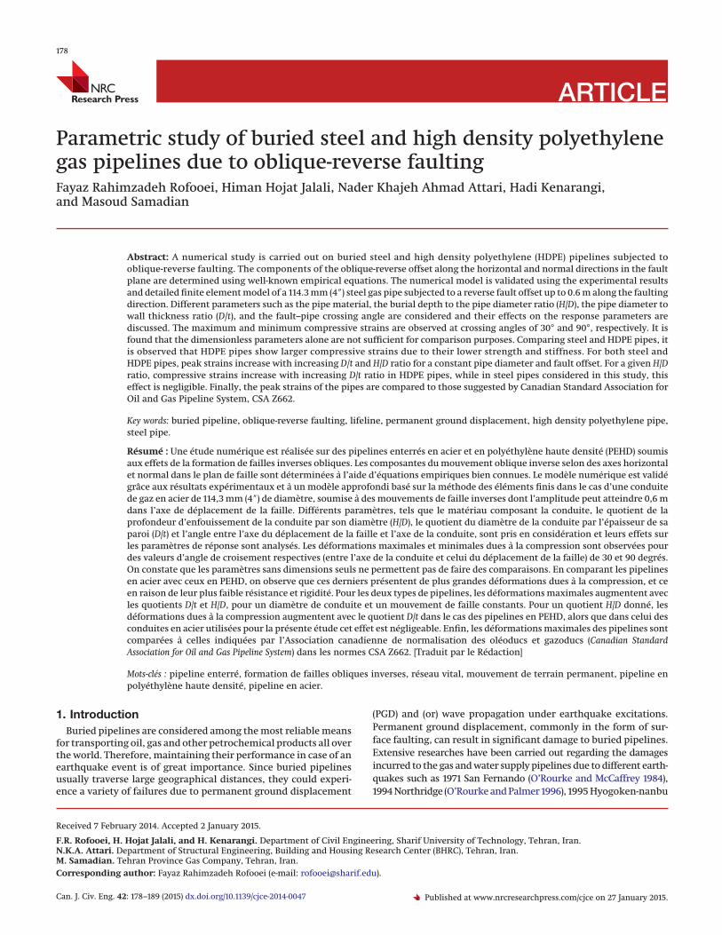
Pipelines could be subjected to different types of faulting such asnormal, reverse, strike-slip or a combination of these faults, referredto as oblique reverse and oblique normal faulting as shown in Fig. 1.Also, depending on the relative orientation of a pipeline with respectto the fault direction, various behaviors like mixed axial compres-sion and bending, or axial tension and bending of the pipes can beexpected. Consequently, different failure types such as tensile rup-ture or wrinkling and buckling may occur. In the case of oblique-reverse faulting, the pipeline is subjected to a three-dimensionalmovement inducing a combined axial compression and bending inthe pipeline. These forces could lead to local buckling of the pipe and(or) warping of the pipe cross section. In case of severe buckling,initiation of rupture failure in pipe could result in fire or other envi-ronmental hazards. Thus, it is essential to study the effect of oblique-reverse faulting on buried pipelines to identify the potential hazards.

A large amount of literature is available on the performance ofburied pipelines subjected to earthquakes. Analytical researchesin this field were initiated by Newmark and Hall (1975), Kennedyet al. (1977), Wang and Yeh (1985) and were extended by Karamitroset al. (2007, 2011) and Trifonov and Cherniy (2010, 2012). Ariman andLee (1992) carried out a parametric study on buried steel pipelinescrossing strike-slip faults using the finite element (FE) method. Intheir numerical analyses, various parameters such as the soil fric-tion angle, pipe diameter, burial depth, and fault–pipe inter-section angle were taken into account. Lee and Bohinsky (1996)studied the behavior of a buried steel pipe crossing a fault withstrike-slip faulting mechanism which resulted in mainly compres-sive strains using FE method. They realized that unlike axial forcethat occurs at the fault location, the peak strains take place at alocation away from the fault plane. Eidinger et al. (2002) evaluatedthe performance of a 2.2 m diameter, steel water pipeline underthe Izmit earthquake 1999 from field observations. They devel-oped a FE model to quantify the response of the same steel pipe-line subjected to a strike-slip fault offset of 3 m and to simulate thefield conditions. Ogawa et al. (2004) used a simple, yet efficientfinite element model to perform a series of nonlinear finite ele-ment analyses on buried gas pipelines subjected to seismic faultdisplacement with special attention to the rupture behavior of thepipelines. Shakib and Zia-Tohidi (2004) studied the behavior ofburied steel pipelines subjected to three-dimensional fault move-ments, considering material and geometrical nonlinearities intheir simple finite element model. Yoshizaki et al. (2003) carriedout an experimental investigation on the effects of PGD on buriedsteel gas distribution pipelines with elbows during earthquakes,using the large split box at Cornell University, and calibrated theirfinite element models for further studies. Ha et al. (2010) per-formed a number of centrifuge tests on buried HDPE pipes understrike-slip faulting. They investigated the effect of faulting direc-tion on these pipelines and compared the results with that of thewell-documented case history presented by Eidinger et al. (2002).Recently, Xie et al. (2011) studied the effect of various parameters

on the behavior of buried HDPE pipelines subjected to strike-slipfaulting using a simple finite element model. They comparedtheir results with those of the centrifuge tests performed atRensselaer Polytechnic Institute by Ha et al. (2008) on HDPE pipes.In another study, Xie et al. (2013) investigated the behavior ofburied HDPE pipes under normal faulting and introduced appro-priate soil–pipe interaction models for normal faulting. Rofooeiet al. (2012) performed a full-scale experiment on a 4== (114.3 mm)steel pipe under reverse faulting of 0.6 m with a dip angle of 61°and developed a three-dimensional FE model that was validatedusing the experimental results.

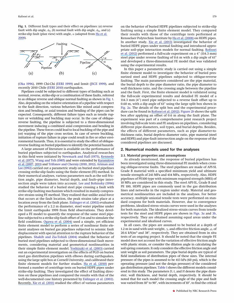
In this paper a parametric study is carried out using a simplefinite element model to investigate the behavior of buried pres-surized steel and HDPE pipelines subjected to oblique-reversefaulting. The main parameters considered are the pipe material,the burial depth to the pipe diameter ratio, the pipe diameter towall thickness ratio, and the crossing angle between the pipelineand the fault. First, the finite element model is validated usingthe full-scale experimental results and detailed FE model of a114.3 mm (4==) steel pipe subjected to a reverse fault offset up to0.60 m, with a dip angle of 61° using the large split box shown inFig. 2a. The details of the split box and the experimental proce-dure can be found in Rofooei et al. (2012). Figure 2b shows the splitbox after applying an offset of 0.6 m along the fault plane. Theexperiment was part of a comprehensive joint research projectinvolving full-scale tests and FE analyses on pipelines, consideringdifferent pipe diameters, soil types, and burial depths. Besides,the effects of different parameters, such as pipe diameter-to-thickness ratio, burial depth-to diameter ratio, pipe material (steeland HDPE) and pipe-fault intersection angle on the response of theconsidered pipelines are discussed.

2. Numerical models used for the analyses

2.1. Material properties and assumptionsAs already mentioned, the response of buried pipelines has

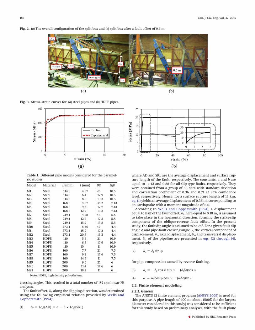
been investigated using three-dimensional FE models when cross-ing oblique-reverse faults. The steel pipelines are made of API-5LGrade B material with a specified minimum yield and ultimatetensile strength of 241 MPa and 414 MPa, respectively. Also, HDPEpipelines of PE100 type with minimum required strength (MRS) of10 MPa are considered in this study. The steel API-5L, Grade B andPE 100, HDPE pipes are commonly used in the gas distributionlines and networks in the region under study. Material and geo-metrical nonlinearities are included in the analyses. For betteraccuracy, multiple uniaxial tensile tests were performed on stan-dard coupons for both materials. However, due to convergenceproblems, idealized stress–strain curves were used in the analysesfor both materials. The idealized stress–strain curves from tensiletests for the steel and HDPE pipes are shown in Figs. 3a and 3b,respectively. They are obtained assuming equal areas under theexperimental and idealized curves.

In all cases, the pipes are assumed to be buried at a depth of1.2 m in sand with unit weight, �, and effective friction angle, �, of20.6 kN/m3 and 38°, respectively. They are obtained from in situtests of an ongoing project. It should be noted that the simple FEmodel does not account for the variation of effective friction anglewith plastic strain, or consider the dilation angle in calculating thesoil spring constants. It only considers the effective friction angle andunit weight as soil parameters. The pipe burial depths are typical offield installations of distribution pipes of these sizes. The internalpressure of the pipes is assumed to be 413 kPa (60 psi), which is theoperating pressure (and not the design pressure) of the consideredgas distribution pipelines. Table 1 shows the different models consid-ered in this study. The parameters D, t, and H denote the pipe diam-eter, wall thickness, and burial depth, respectively. It should benoted that for each model the crossing angle of the pipe and faultwas varied from 10° to 90°, with increments of 10°, to find the critical

Fig. 1. Different fault types and their effect on pipelines: (a) reversefault with dip angle, �T, (b) normal fault with dip angle, �N, and (c)strike-slip fault (plan view) with angle, � (adapted from Ha et al.2008).

Rafooei et al. 179

Published by NRC Research Press

crossing angles. This resulted in a total number of 189 nonlinear FEanalyses.

The fault offset, �f, along the slipping direction, was determinedusing the following empirical relation provided by Wells andCoppersmith (1994):

(1) �f � Log(AD) � a � b × Log(SRL)

where AD and SRL are the average displacement and surface rup-ture length of the fault, respectively. The constants, a and b areequal to −1.43 and 0.88 for all-slip-type faults, respectively. Theywere obtained from a group of 66 data with standard deviationand correlation coefficient of 0.36 and 0.71 at 95% confidencelevel, respectively. Hence, for a surface rupture length of 13 km,eq. (1) yields an average displacement of 0.36 m, corresponding toan earthquake with a moment magnitude of 6.6.

According to Wells and Coppersmith (1994), a displacementequal to half of the fault offset, �f, here equal to 0.18 m, is assumedto take place in the horizontal direction, forming the strike-slipcomponent of the oblique-reverse fault offset. In the presentstudy, the fault dip angle is assumed to be 75°. For a given fault dipangle � and pipe-fault crossing angle �, the vertical component ofdisplacement, �v, axial displacement, �a, and transversal displace-ment, �t, of the pipeline are presented in eqs. (2) through (4),respectively.

(2) �v � �f sin �

for pipe compression caused by reverse faulting,

(3) �a � �f cos � sin � (�f/2)cos �

(4) �t � �f cos � cos � (�f/2)sin �

2.2. Finite element modeling

2.2.1. GeneralThe ANSYS 12 finite element program (ANSYS 2009) is used for

this purpose. A pipe length of 400 m (about 1500D for the largestdiameter considered in this study) was considered to be sufficientfor this study based on preliminary analyses, with the fault plane

Fig. 2. (a) The overall configuration of the split box and (b) split box after a fault offset of 0.6 m.

Fig. 3. Stress–strain curves for: (a) steel pipes and (b) HDPE pipes.

Table 1. Different pipe models considered for the paramet-ric studies.

Model Material D (mm) t (mm) D/t H/D

M1 Steel 114.3 4.37 26 10.5M2 Steel 114.3 6.4 17.9 10.5M3 Steel 114.3 8.6 13.3 10.5M4 Steel 168.3 4.37 38.2 7.13M5 Steel 168.3 9.5 17.7 7.13M6 Steel 168.3 12.7 13.3 7.13M7 Steel 219.1 4.78 46 5.5M8 Steel 219.1 12.7 17.3 5.5M9 Steel 219.1 15.9 13.8 5.5M10 Steel 273.1 5.56 49 4.4M11 Steel 273.1 15.9 17.2 4.4M12 Steel 273.1 20.6 13.3 4.4M13 HDPE 110 5.3 21 10.9M14 HDPE 110 6.3 17.6 10.9M15 HDPE 110 10 11 10.9M16 HDPE 160 7.7 21 7.5M17 HDPE 160 9.1 17.6 7.5M18 HDPE 160 14.6 11 7.5M19 HDPE 200 9.6 21 6M20 HDPE 200 11.4 17.6 6M21 HDPE 200 18.2 11 6

Note: HDPE, high density polyethylene.

180 Can. J. Civ. Eng. Vol. 42, 2015

Published by NRC Research Press

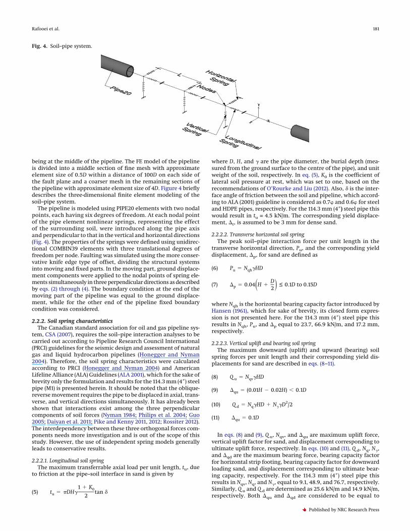
being at the middle of the pipeline. The FE model of the pipelineis divided into a middle section of fine mesh with approximateelement size of 0.5D within a distance of 100D on each side ofthe fault plane and a coarser mesh in the remaining sections ofthe pipeline with approximate element size of 4D. Figure 4 brieflydescribes the three-dimensional finite element modeling of thesoil–pipe system.

The pipeline is modeled using PIPE20 elements with two nodalpoints, each having six degrees of freedom. At each nodal pointof the pipe element nonlinear springs, representing the effectof the surrounding soil, were introduced along the pipe axisand perpendicular to that in the vertical and horizontal directions(Fig. 4). The properties of the springs were defined using unidirec-tional COMBIN39 elements with three translational degrees offreedom per node. Faulting was simulated using the more conser-vative knife edge type of offset, dividing the structural systemsinto moving and fixed parts. In the moving part, ground displace-ment components were applied to the nodal points of spring ele-ments simultaneously in three perpendicular directions as describedby eqs. (2) through (4). The boundary condition at the end of themoving part of the pipeline was equal to the ground displace-ment, while for the other end of the pipeline fixed boundarycondition was considered.

2.2.2. Soil spring characteristicsThe Canadian standard association for oil and gas pipeline sys-

tem, CSA (2007), requires the soil–pipe interaction analyses to becarried out according to Pipeline Research Council International(PRCI) guidelines for the seismic design and assessment of naturalgas and liquid hydrocarbon pipelines (Honegger and Nyman2004). Therefore, the soil spring characteristics were calculatedaccording to PRCI (Honegger and Nyman 2004) and AmericanLifeline Alliance (ALA) Guidelines (ALA 2001), which for the sake ofbrevity only the formulation and results for the 114.3 mm (4==) steelpipe (M1) is presented herein. It should be noted that the oblique-reverse movement requires the pipe to be displaced in axial, trans-verse, and vertical directions simultaneously. It has already beenshown that interactions exist among the three perpendicularcomponents of soil forces (Nyman 1984; Philips et al. 2004; Guo2005; Daiyan et al. 2011; Pike and Kenny 2011, 2012; Rossiter 2012).The interdependency between these three orthogonal forces com-ponents needs more investigation and is out of the scope of thisstudy. However, the use of independent spring models generallyleads to conservative results.

2.2.2.1. Longitudinal soil springThe maximum transferrable axial load per unit length, tu, due

to friction at the pipe–soil interface in sand is given by

(5) tu � DH�1 � K0

2tan �

where D, H, and � are the pipe diameter, the burial depth (mea-sured from the ground surface to the centre of the pipe), and unitweight of the soil, respectively. In eq. (5), K0 is the coefficient oflateral soil pressure at rest, which was set to one, based on therecommendations of O’Rourke and Liu (2012). Also, � is the inter-face angle of friction between the soil and pipeline, which accord-ing to ALA (2001) guideline is considered as 0.7� and 0.6� for steeland HDPE pipes, respectively. For the 114.3 mm (4==) steel pipe thiswould result in tu = 4.5 kN/m. The corresponding yield displace-ment, �t, is assumed to be 3 mm for dense sand.

2.2.2.2. Transverse horizontal soil springThe peak soil–pipe interaction force per unit length in the

transverse horizontal direction, Pu, and the corresponding yielddisplacement, �p, for sand are defined as

(6) Pu � Nqh�HD

(7) �p � 0.04�H �D2 � ≤ 0.1D to 0.15D

where Nqh is the horizontal bearing capacity factor introduced byHansen (1961), which for sake of brevity, its closed form expres-sion is not presented here. For the 114.3 mm (4==) steel pipe thisresults in Nqh, Pu, and �p equal to 23.7, 66.9 kN/m, and 17.2 mm,respectively.

2.2.2.3. Vertical uplift and bearing soil springThe maximum downward (uplift) and upward (bearing) soil

spring forces per unit length and their corresponding yield dis-placements for sand are described in eqs. (8–11).

(8) Q u � Nqv�HD

(9) �qu � (0.01H 0.02H) � 0.1D

(10) Q d � Nq�HD � N��D2/2

(11) �qu � 0.1D

In eqs. (8) and (9), Q u, Nqv, and �qu are maximum uplift force,vertical uplift factor for sand, and displacement corresponding toultimate uplift force, respectively. In eqs. (10) and (11), Q d, Nq, N�,and �qd are the maximum bearing force, bearing capacity factorfor horizontal strip footing, bearing capacity factor for downwardloading sand, and displacement corresponding to ultimate bear-ing capacity, respectively. For the 114.3 mm (4==) steel pipe thisresults in Nqv, Nq, and N�, equal to 9.1, 48.9, and 76.7, respectively.Similarly, Q u and Q d are determined as 25.6 kN/m and 14.9 kN/m,respectively. Both �qu and �qd are considered to be equal to

Fig. 4. Soil–pipe system.

Rafooei et al. 181

Published by NRC Research Press

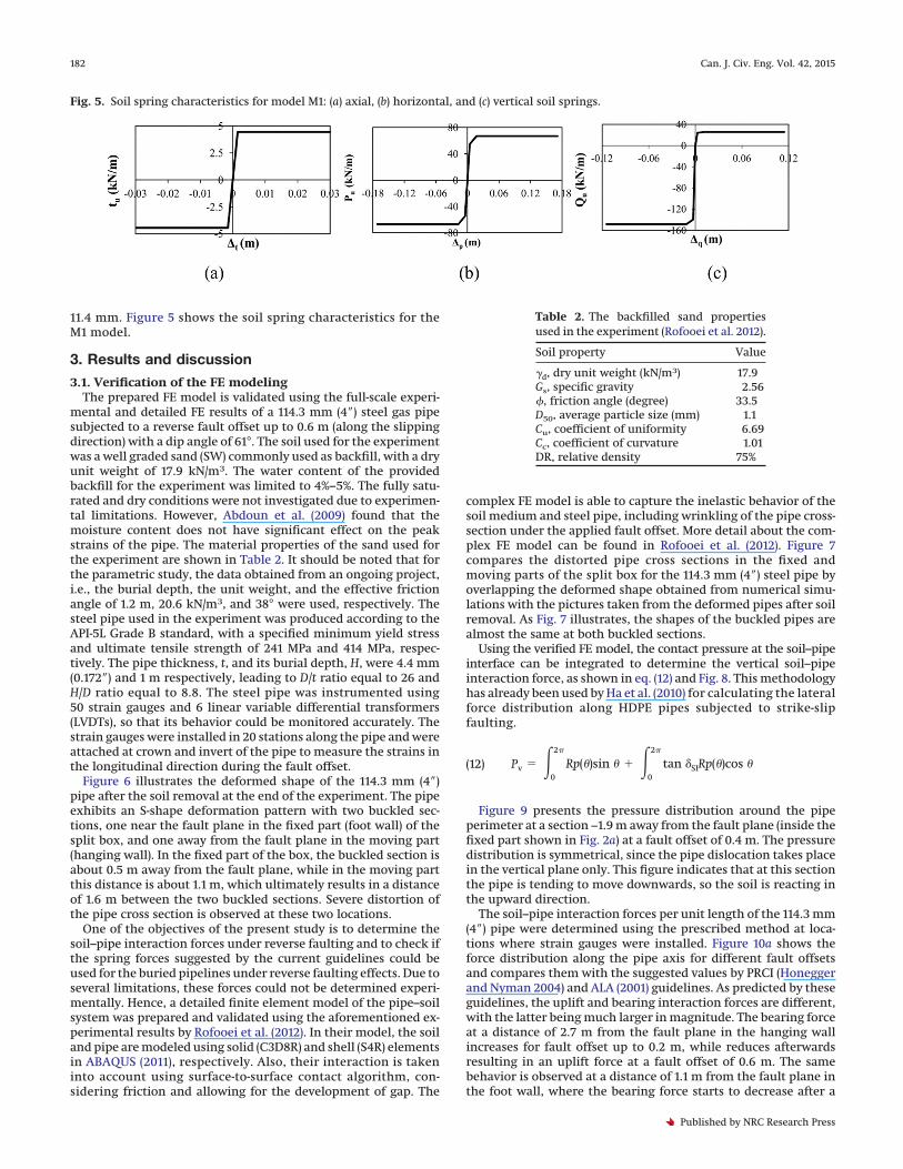
11.4 mm. Figure 5 shows the soil spring characteristics for theM1 model.

3. Results and discussion

3.1. Verification of the FE modelingThe prepared FE model is validated using the full-scale experi-

mental and detailed FE results of a 114.3 mm (4==) steel gas pipesubjected to a reverse fault offset up to 0.6 m (along the slippingdirection) with a dip angle of 61°. The soil used for the experimentwas a well graded sand (SW) commonly used as backfill, with a dryunit weight of 17.9 kN/m3. The water content of the providedbackfill for the experiment was limited to 4%–5%. The fully satu-rated and dry conditions were not investigated due to experimen-tal limitations. However, Abdoun et al. (2009) found that themoisture content does not have significant effect on the peakstrains of the pipe. The material properties of the sand used forthe experiment are shown in Table 2. It should be noted that forthe parametric study, the data obtained from an ongoing project,i.e., the burial depth, the unit weight, and the effective frictionangle of 1.2 m, 20.6 kN/m3, and 38° were used, respectively. Thesteel pipe used in the experiment was produced according to theAPI-5L Grade B standard, with a specified minimum yield stressand ultimate tensile strength of 241 MPa and 414 MPa, respec-tively. The pipe thickness, t, and its burial depth, H, were 4.4 mm(0.172==) and 1 m respectively, leading to D/t ratio equal to 26 andH/D ratio equal to 8.8. The steel pipe was instrumented using50 strain gauges and 6 linear variable differential transformers(LVDTs), so that its behavior could be monitored accurately. Thestrain gauges were installed in 20 stations along the pipe and wereattached at crown and invert of the pipe to measure the strains inthe longitudinal direction during the fault offset.

Figure 6 illustrates the deformed shape of the 114.3 mm (4==)pipe after the soil removal at the end of the experiment. The pipeexhibits an S-shape deformation pattern with two buckled sec-tions, one near the fault plane in the fixed part (foot wall) of thesplit box, and one away from the fault plane in the moving part(hanging wall). In the fixed part of the box, the buckled section isabout 0.5 m away from the fault plane, while in the moving partthis distance is about 1.1 m, which ultimately results in a distanceof 1.6 m between the two buckled sections. Severe distortion ofthe pipe cross section is observed at these two locations.

One of the objectives of the present study is to determine thesoil–pipe interaction forces under reverse faulting and to check ifthe spring forces suggested by the current guidelines could beused for the buried pipelines under reverse faulting effects. Due toseveral limitations, these forces could not be determined experi-mentally. Hence, a detailed finite element model of the pipe–soilsystem was prepared and validated using the aforementioned ex-perimental results by Rofooei et al. (2012). In their model, the soiland pipe are modeled using solid (C3D8R) and shell (S4R) elementsin ABAQUS (2011), respectively. Also, their interaction is takeninto account using surface-to-surface contact algorithm, con-sidering friction and allowing for the development of gap. The

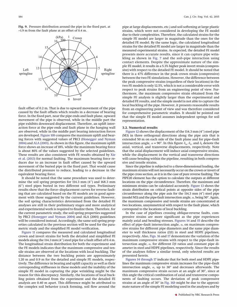
complex FE model is able to capture the inelastic behavior of thesoil medium and steel pipe, including wrinkling of the pipe cross-section under the applied fault offset. More detail about the com-plex FE model can be found in Rofooei et al. (2012). Figure 7compares the distorted pipe cross sections in the fixed andmoving parts of the split box for the 114.3 mm (4==) steel pipe byoverlapping the deformed shape obtained from numerical simu-lations with the pictures taken from the deformed pipes after soilremoval. As Fig. 7 illustrates, the shapes of the buckled pipes arealmost the same at both buckled sections.

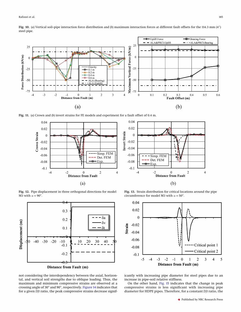
Using the verified FE model, the contact pressure at the soil–pipeinterface can be integrated to determine the vertical soil–pipeinteraction force, as shown in eq. (12) and Fig. 8. This methodologyhas already been used by Ha et al. (2010) for calculating the lateralforce distribution along HDPE pipes subjected to strike-slipfaulting.

(12) Pv � �0

2

Rp( )sin � �0

2

tan �SIRp( )cos

Figure 9 presents the pressure distribution around the pipeperimeter at a section −1.9 m away from the fault plane (inside thefixed part shown in Fig. 2a) at a fault offset of 0.4 m. The pressuredistribution is symmetrical, since the pipe dislocation takes placein the vertical plane only. This figure indicates that at this sectionthe pipe is tending to move downwards, so the soil is reacting inthe upward direction.

The soil–pipe interaction forces per unit length of the 114.3 mm(4==) pipe were determined using the prescribed method at loca-tions where strain gauges were installed. Figure 10a shows theforce distribution along the pipe axis for different fault offsetsand compares them with the suggested values by PRCI (Honeggerand Nyman 2004) and ALA (2001) guidelines. As predicted by theseguidelines, the uplift and bearing interaction forces are different,with the latter being much larger in magnitude. The bearing forceat a distance of 2.7 m from the fault plane in the hanging wallincreases for fault offset up to 0.2 m, while reduces afterwardsresulting in an uplift force at a fault offset of 0.6 m. The samebehavior is observed at a distance of 1.1 m from the fault plane inthe foot wall, where the bearing force starts to decrease after a

Fig. 5. Soil spring characteristics for model M1: (a) axial, (b) horizontal, and (c) vertical soil springs.

Table 2. The backfilled sand propertiesused in the experiment (Rofooei et al. 2012).

Soil property Value

�d, dry unit weight (kN/m3) 17.9Gs, specific gravity 2.56�, friction angle (degree) 33.5D50, average particle size (mm) 1.1Cu, coefficient of uniformity 6.69Cc, coefficient of curvature 1.01DR, relative density 75%

182 Can. J. Civ. Eng. Vol. 42, 2015

Published by NRC Research Press

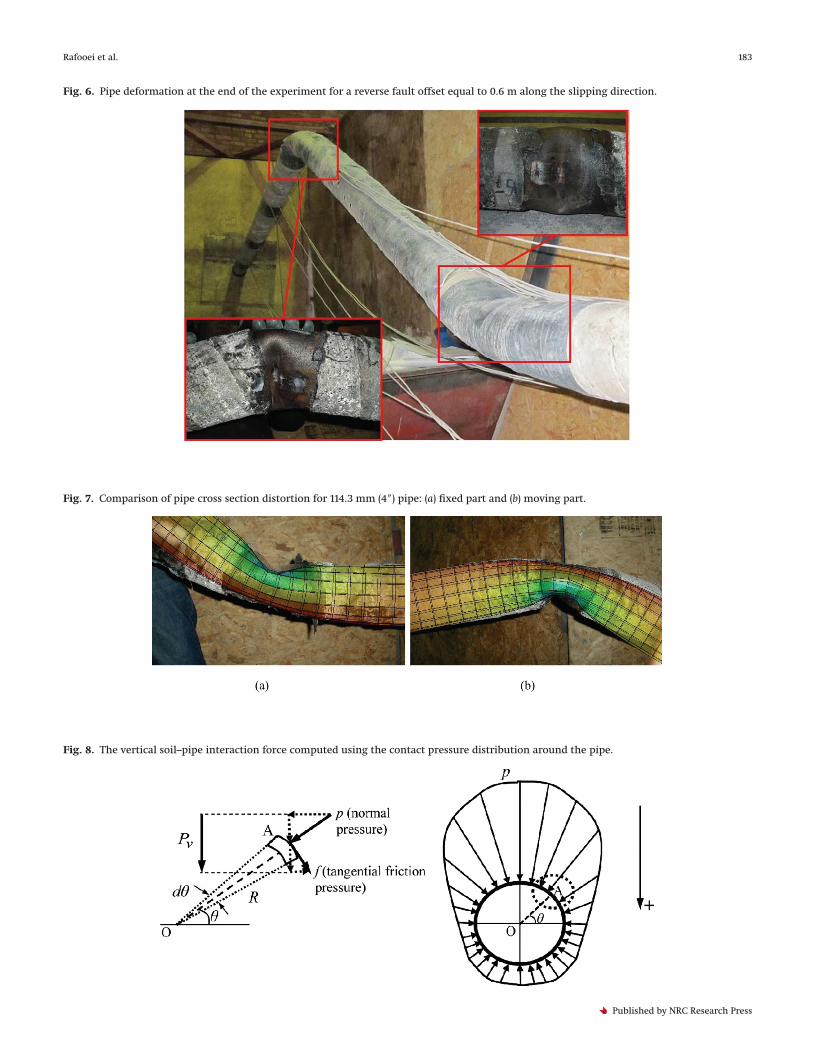
Fig. 6. Pipe deformation at the end of the experiment for a reverse fault offset equal to 0.6 m along the slipping direction.

Fig. 7. Comparison of pipe cross section distortion for 114.3 mm (4==) pipe: (a) fixed part and (b) moving part.

Fig. 8. The vertical soil–pipe interaction force computed using the contact pressure distribution around the pipe.

Rafooei et al. 183

Published by NRC Research Press

fault offset of 0.2 m. That is due to upward movement of the pipecaused by the fault offsets which results in a decrease of bearingforce. In the fixed part, near the pipe ends and fault plane, upwardmovement of the pipe is observed, while in the middle part thepipe exhibits downward displacement. Therefore, an uplift inter-action force at the pipe ends and fault plane in the hanging wallare observed, while in the middle part bearing interaction forcesare developed. Figure 10b compares the maximum uplift and bear-ing forces with suggested values of PRCI (Honegger and Nyman2004) and ALA (2001). As shown in this figure, the maximum upliftforce shows an increase of 18%, while the maximum bearing forceis about 80% of the values suggested by the selected guidelines.These results are also consistent with FE results obtained by Xieet al. (2013) for normal faulting. The maximum bearing force re-duces due to an increase in fault offset caused by the upwardmovement of the buried pipe in the fixed part. That would causethe distributed pressure to reduce, leading to a decrease in theequivalent bearing force.

It should be noted that the same procedure was used to deter-mine the soil spring properties for 114.3 mm (4==) and 168.3 mm(6==) steel pipes buried in two different soil types. Preliminaryresults show that the force–displacement curves for reverse fault-ing that are calculated based on the FE models are in good agree-ment with those suggested by the current guidelines. However,the soil spring characteristics determined from the detailed FEanalyses are still in their preliminary stages and more analyticaland experimental work is required to finalize them. Therefore, forthe current parametric study, the soil spring properties suggestedby PRCI (Honegger and Nyman 2004) and ALA (2001) guidelineswill be considered instead. Accordingly, the same soil spring prop-erties calculated in the previous section will be used for the para-metric study and the simplified FE model verification.

Figure 11 compares the measured and calculated longitudinalcrown and invert strains for both the detailed and simplified FEmodels along the 114.3 mm (4==) steel pipe for a fault offset of 0.4 m.The longitudinal strain distribution for both the experiment andthe FE models indicates that the maximum compressive and ten-sile strains are observed at the locations with local buckling. Thedistance between the two buckling points are approximately1.20 m and 0.9 m for the detailed and simple FE models, respec-tively. The difference in bearing and uplift capacity as well as theircorresponding stiffnesses in these models and the inability of thesimple FE model in capturing the pipe wrinkling might be thereason for this discrepancy. Similarly, the locations of local buck-ling points obtained from the experiment and the detailed FEanalysis are 0.40 m apart. This difference might be attributed tothe complex soil behavior (crack forming, soil flow around the

pipe at large displacements, etc.) and soil softening at large plasticstrains, which were not considered in developing the FE modeldue to their complexities. Therefore, the calculated strains for thesimple FE model are larger in magnitude than the ones for thedetailed FE model. By the same logic, the calculated longitudinalstrains for the detailed FE model are larger in magnitude than themeasured experimental strains. As expected, the detailed FE modelpresents more accurate results, since it can capture pipe wrin-kling as shown in Fig. 7 and the soil–pipe interaction usingcontact elements. Despite the approximate nature of the sim-ple FE model, it results in a 5.3% higher peak invert strain (compres-sive) with respect to the detailed FE model. It should be noted thatthere is a 47% difference in the peak crown strain (compressive)between the two FE simulations. However, the difference betweenthe peak compressive strains (regardless of their locations) in thetwo FE models is only 12.5%, which is not a considerable error withrespect to peak strains from an engineering point of view. Fur-thermore, the maximum compressive strain obtained from thesimple FE analysis is slightly larger than the experimental anddetailed FE results, and the simple model is not able to capture thelocal buckling of the pipe. However, it presents reasonable resultsfrom an engineering point of view and was therefore consideredfor comprehensive parametric studies. It should be pointed outthat the simple FE model assumes independent springs for soilrepresentation.

3.2. Numerical resultsFigure 12 shows the displacement of the 114.3 mm (4==) steel pipe

(M3) in three orthogonal directions along the pipe axis that isextended 50 m on each side of the fault plane and for pipe–faultintersection angle, � = 90°. In this figure �a, �v, and �t denote theaxial, vertical, and transverse displacements, respectively. Notethat the axial displacement will induce axial compressive strains,while the displacement in the vertical and transverse directionswill cause bending within the pipeline, resulting in both compres-sive and tensile strains.

Since the pipeline is subjected to a three-dimensional loading, themaximum strains will not necessarily occur on the crown or invert ofthe pipe cross section, as it is in the case of pure reverse faulting. ThePIPE20 element has the option to calculate the outputs at differentlocations on the pipe circumference. Therefore, the maximum andminimum strains can be calculated accurately. Figure 13 shows thestrain distribution on critical points at opposite sides of the pipecircumference along the pipe axis for the 114.3 mm (4==) steel pipe(model M3) and the pipe-fault intersection angle, �, being 50°. Again,the maximum compressive and tensile strains are concentrated attwo locations, unsymmetrical with respect to the fault plane, whichcorrespond to the locations of local buckling.

In the case of pipelines crossing oblique-reverse faults, com-pressive strains are more significant as the pipe experiencesmainly axial and bending stresses. Figures 14 and 15 describe theeffect of pipe–fault intersection angle, �, on maximum compres-sive strains for different pipe diameters and the same pipe diam-eter to wall thickness ratios (D/t) in steel and HDPE pipelines,respectively. Also, Figs. 16 and 17 demonstrate the variation of themaximum compressive strains with respect to the pipe–fault in-tersection angle, �, for different D/t ratios and constant pipe di-ameter in steel and HDPE pipelines, respectively. Since the resultsof the analyses follow a similar trend, only selected results arepresented herein.

Figures 14 through 17 indicate that for both steel and HDPE pipe-lines the maximum compressive strain increases for the pipe–faultintersection angle, �, up to 30° and decreases afterwards. Themaximum compressive strain occurs at an angle of 30°, since atthis angle the critical combination of axial and transverse compo-nents of faulting occurs. The deviation of peak compressivestrains at an angle of 30° in Fig. 16b might be due to the approxi-mate nature of the simple FE modeling used in the analyses and by

Fig. 9. Pressure distribution around the pipe in the fixed part, at−1.9 m from the fault plane at an offset of 0.4 m.

184 Can. J. Civ. Eng. Vol. 42, 2015

Published by NRC Research Press

not considering the interdependency between the axial, horizon-tal, and vertical soil strengths due to oblique loading. Thus, themaximum and minimum compressive strains are observed at acrossing angle of 30° and 90°, respectively. Figure 14 indicates thatfor a given D/t ratio, the peak compressive strains decrease signif-

icantly with increasing pipe diameter for steel pipes due to anincrease in pipe–soil relative stiffness.

On the other hand, Fig. 15 indicates that the change in peakcompressive strains is less significant with increasing pipediameter for HDPE pipes. Therefore, for a constant D/t ratio, the

Fig. 10. (a) Vertical soil–pipe interaction force distribution and (b) maximum interaction forces at different fault offsets for the 114.3 mm (4==)steel pipe.

Fig. 11. (a) Crown and (b) invert strains for FE models and experiment for a fault offset of 0.4 m.

Fig. 12. Pipe displacement in three orthogonal directions for modelM3 with � = 90°.

Fig. 13. Strain distribution for critical locations around the pipecircumference for model M3 with � = 50°.

Rafooei et al. 185

Published by NRC Research Press

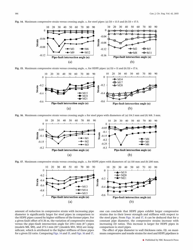
amount of reduction in compressive strain with increasing pipediameter is significantly larger for steel pipes in comparison tothe HDPE pipes caused by higher stiffness of the former pipes. Fora given fault offset of 0.36 m, the variation of compressive strainsversus the pipe–fault intersection angle for 219.1 mm (8==) pipes(models M8, M9), and 273.1 mm (10==) (models M11, M12) are insig-nificant, which is attributed to the higher stiffness of these pipesfor a given D/t ratio. Comparing Figs. 14 and 15, and Figs. 16 and 17,

one can conclude that HDPE pipes exhibit larger compressivestrains due to their lower strength and stiffness with respect tothe steel pipes. From Figs. 16 and 17, it can be deduced that for aconstant pipe diameter, the compressive strains increase withincreasing D/t ratios. This increase is larger for HDPE pipes incomparison to steel pipes.

The effect of pipe diameter to wall thickness ratio, D/t, on maxi-mum compressive and tensile strains for steel and HDPE pipelines is

Fig. 14. Maximum compressive strain versus crossing angle, �, for steel pipes: (a) D/t ≈ 13.5 and (b) D/t ≈ 17.5.

Fig. 15. Maximum compressive strain versus crossing angle, �, for HDPE pipes: (a) D/t = 11 and (b) D/t = 17.6.

Fig. 16. Maximum compressive strain versus crossing angle � for steel pipes with diameters of: (a) 114.3 mm and (b) 168. 3 mm.

Fig. 17. Maximum compressive strain versus crossing angle, �, for HDPE pipes with diameters of: (a) 110 mm and (b) 200 mm.

186 Can. J. Civ. Eng. Vol. 42, 2015

Published by NRC Research Press

shown in Fig. 18. One could observe that regardless of the pipe ma-terial, by increasing D/t ratio, both compressive and tensile strainstend to increase for a given fault offset and pipe diameter. Also for agiven D/t ratio, maximum strains decrease with increasing pipe di-ameter due to higher stiffness of these pipes. Again, this effect ismore significant for steel pipes in comparison to the HDPE pipes. Byevaluating the obtained results for M4, M7, and M10 models as well asM14 and M19 ones, it can be concluded that despite increasing D/tratio, the maximum strains were decreased. This is due to the factthat M10 has a larger pipe diameter and higher stiffness compared toM4 and M7. Thus, before drawing any general conclusion by compar-ing the results from different D/t ratios, one of the parameters, eitherD or t, should be kept constant. Otherwise, comparison betweendifferent D/t ratios with different diameters and (or) thicknessescould lead to erroneous conclusions.

Figure 19 presents the effect of burial depth to pipe diameterratio, H/D, on compressive strains for different D/t ratios. As it isshown in this figure, for both steel and HDPE pipelines and for agiven burial depth, increasing H/D would result in an increase inthe compressive strains. However, the variation of compressivestrains with H/D is more significant for steel pipes in comparisonto the HDPE pipes in which this effect is negligible, especially forlower D/t ratios. For a given H/D ratio, compressive strains increasewith increasing D/t ratio in HDPE pipes, while in steel pipes thiseffect is negligible. That could be attributed to the definition ofHDPE as an almost elastic – perfectly plastic material, while thesteel material exhibits hardening behavior. Therefore, the plasticstrain rate will significantly increase after yielding for HDPE pipesin comparison to steel pipes. This is the reason for the differencesthat exist in the strains of steel and HDPE pipes with differentD/t ratios. It should be noted that before drawing any conclusionby comparing the results for different H/D ratios, one of the pa-rameters, H or D should be kept constant (Fig. 19b, for models M14,M15, M16).

According to the CSA (2007) Z662 standard, the tensile strainlimit for preventing rupture in the pipe, including surface-breakingdefects, which is assumed to happen in the girth welds, can beobtained from

(13) �tcrit � �(2.361.58�0.101��)(1 � 16.1�4.45)

× (0.157 � 0.239�0.241�0.315)

where �tcrit is the tensile strain capacity (%), � is the crack tip

opening displacement (CTOD) toughness of the weld (mm), � isthe ratio of yield to tensile strength, � is the defect length to pipewall thickness ratio, and � is the defect height to pipe wall thick-ness ratio. Equation (13) is valid for: 0.1 ≤ � ≤ 0.3, 0.7 ≤ � ≤0.95, 1 ≤ � ≤ 10, and � ≤ 0.5. For a pipe with minor defects, one canassume � � 0.1, � � 0.7, � � 1, and � � 0.1, and the tensile straincapacity can be accordingly determined as 1.5%, which is some-what more conservative than the suggested value of 2% by ALA

(2001). The CSA (2007) Z662 and ALA (2001) do not consider anytensile strain limit for HDPE pipes. The Indian Institute of Tech-nology in Kanpur (IITK) Guidelines for Seismic Design of BuriedPipelines (2007) funded by the Gujarat State Disaster ManagementAuthority (GSDMA) (IITK-GSDMA 2007) limits the tensile strain to20% for polyethylene pipelines.

The compressive strain capacity of the pipe for the operatingpressure of 413 kPa can be obtained from eq. (14), which wasinitially proposed by Gresnigt (1986)

(14) �ccrit � 0.5� t

D� 0.0025 � 3000�(pi pe)D

2tE�2

where pi, pe, and E denote the internal and external pipe pressureand the pipe modulus of elasticity, respectively. Although eq. (14)has originally been developed for steel pipes (Gresnigt 1986; CSA2007; ALA 2001), it is also used for estimating the buckling strainof HDPE pipes, since there is no criterion in this regard in theliterature to the knowledge of the authors. Table 3 shows thecritical compressive strains versus D/t ratio for the pipelines con-sidered in the current study.

Considering the abovementioned acceptance criteria for tensileand compressive strains, only steel pipelines with diameters of219.1 mm (8==) and D/t equal to 13.8 (model M9) and 17.3 (model M8),as well as steel pipelines with diameter of 273.1 mm (10==) and D/tequal to 13.3 (model M12) and 17.2 (model M11) can remain func-tional when subjected to a fault offset of 0.36 m. Thus, it can beconcluded that based on the prescribed acceptance criteria, ex-cept for models M8, M9, M11, M12, the considered pipelines arevulnerable to moderate amount of oblique reverse faulting. Also,considering the results obtained from the parametric studies, thebest way to enhance the performance of gas pipelines with lowerD/t and H/D ratios is to place them, preferably, at right angle withrespect to the fault plane at locations near the fault zone.

4. Summary and conclusionsA parametric study was conducted on pressurized buried gas

pipelines subjected to oblique-reverse faulting of 0.36 m bymeans of a simple finite element model, where the pipe andsoil springs were modeled using discrete pipe and nonlinearspring elements from the ANSYS 12 library (ANSYS 2009), respec-tively. In all cases, the pipes were assumed to be buried at a depthof 1.2 m in sand with unit weight, �, and effective friction angle, �,of 20.6 kN/m3 and 38°, respectively. The values were obtainedfrom in situ tests of an ongoing project. The soil spring propertieswere determined according to PRCI (Honegger and Nyman 2004)and ALA (2001) guidelines as required per clause C.8.10 of CSAZ662 (CSA 2007). The internal pressure was assumed to be equal to413 kPa (60 psi), as the operating pressure for the considered gasdistribution network. A simple finite element model was devel-oped and validated using experimental and detailed FE results of

Fig. 18. Maximum strain versus D/t ratio for: (a) steel and (b) HDPE pipes.

Rafooei et al. 187

Published by NRC Research Press

a 114.3 mm (4==) steel pipe subjected to a reverse fault with an offsetup to 0.6 m along the slipping direction. A brief description of theexperiment as well as the detailed finite element study and theirresults were presented and the soil–pipe interaction forces ob-tained from the detailed FE model is compared to those sug-gested by PRCI (Honegger and Nyman 2004) and ALA (2001)guidelines. It is found that the detailed FE model, which is able tocapture the pipe wrinkling, presents more accurate results, re-garding the induced strains and the location of the buckledsections. However, since the difference between the peak com-pressive strains in the two FE models was not significant from anengineering point of view (only 12.5% regardless of their location),the simple FE model was considered for the comprehensive para-metric studies. Also, the spring properties suggested by PRCI(Honegger and Nyman 2004) and ALA (2001) were considered inmodeling the soil–pipe interaction. It should be noted that theinterdependency among axial-lateral and vertical soil restraintand its effects on the results needs more experimental and numer-ical investigation. Parameters considered in this study were thepipe material (steel and HDPE), the burial depth to the pipe diam-eter (H/D) ratio, the pipe diameter to wall thickness (D/t) ratio, andthe pipe-fault intersection angle (�). Both material and geometri-cal nonlinearities were considered in the analyses. Based on theresults of a large number of nonlinear finite element analyses thefollowing conclusions are made:

(1) The maximum and minimum compressive strains are ob-served at crossing angles of 30° and 90°, respectively. Thus, fornew pipelines to be subjected to oblique-reverse faulting, it isimportant to place the pipeline at right angle with respect tofault plane.

(2) HDPE pipes exhibit larger compressive strains due to theirlower strength and stiffness.

(3) When comparing the results for different D/t and (or) H/D ratios,one of the parameters, either D, t or H, should be kept constantbefore any general remark is made. In other words the dimension-less parameters (D/t and H/D) alone are not sufficient for compar-ison purposes, and the relative stiffness of the pipe should betaken into account as well.

(4) For a constant D/t ratio, the compressive strains reduce withincreasing pipe diameter. The amount of reduction in compres-sive strain with increasing pipe diameter is significantly larger forsteel pipes in comparison to the HDPE pipes, due to their higherstrength and stiffness.

(5) For a constant pipe diameter, the compressive strains in-crease with increasing D/t ratios. This increase is larger for HDPEpipes compared to steel pipes.

(6) For both steel and HDPE pipelines, the maximum compres-sive and tensile strains increase with increasing D/t ratio for agiven fault offset and pipe diameter. From an application point ofview, only pipes with low D/t ratios should be used in the vicinityof the fault zone.

(7) For both steel and HDPE pipelines, with increasing H/D ratiothe compressive strains increase for a given pipe diameter andfault offset. Again, it can be suggested that the pipes be buried ata shallow depth in the vicinity of the fault zone to minimize thecompressive strains.

(8) The variation of compressive strains with increasingH/D ratio is more significant for steel pipes compared to HDPEpipes. In the HDPE pipes, this effect is negligible, especially forlower D/t ratios.

(9) For a given H/D ratio, compressive strains increase with in-creasing D/t ratio in HDPE pipes, while in steel pipes considered inthis study, this effect is negligible. That could be attributed to thedefinition of HDPE as an almost elastic – perfectly plastic material,while the steel material exhibits hardening behavior. Therefore,the plastic strain rate will significantly increase after yielding forHDPE pipes in comparison to steel pipes.

AcknowledgementsThe work presented herein is part of an extensive experimental

and numerical project performed by Sharif University of Technol-ogy. The authors wish to thank the Research Bureau of the TehranProvince Gas Company for its valuable financial support and as-sistance.

ReferencesABAQUS. 2011. Users’ manual. Simulia, Providence, RI, USA.Abdoun, T.H., Ha, D., O’Rourke, M.J., Symans, M.D., O’Rourke, T.D., Palmer, M.C.,

and Stewart, H.E. 2009. Factors influencing the behavior of buried pipelinessubjected to earthquake faulting. Soil Dynamics and Earthquake Engineer-ing, 29(3): 415–427. doi:10.1016/j.soildyn.2008.04.006.

ALA. 2001. Guidelines for the design of buried steel pipes. American LifelineAlliance, American Society of Civil Engineers, and Federal Emergency Man-agement Agency, USA.

ANSYS. 2009. User’s manual. Version 12.1. ANSYS Inc., Houston, TX, USA.Ariman, T., and Lee, B.J. 1992. Tension/bending behavior of buried pipelines

subject to fault movements in earthquakes. In Proceedings of the 10th

World Conference on Earthquake Engineering, Madrid, Spain, 19–24 July.pp. 5423–5426.

CSA. 2007. CSA-Z662-07 - oil and gas pipeline systems. Canadian Standard Asso-ciation, Mississauga, Ont.

Daiyan, N., Kenny, S., Phillips, R., and Popescu, R. 2011. Investigating pipeline-soil interaction under axial-lateral relative movements in sand. CanadianGeotechnical Journal, 48(11): 1683–1695. doi:10.1139/t11-061.

EERI. 1999. The Chi-Chi, Taiwan Earthquake of September 21, 1999. EarthquakeEngineering Research Institute, Special Earthquake Report.

Fig. 19. Maximum compressive strain versus H/D for: (a) steel and (b) HDPE pipes.

Table 3. Compressive strain capacities for different pipes considered in this study.

D/t 11 13.3 13.8 17.2 17.3 17.6 17.7 17.9 21 26 38 46 49

�cr (%) 4.87 3.51 3.37 2.66 2.64 4.06 2.57 2.54 4.21 1.67 1.07 0.84 0.77

188 Can. J. Civ. Eng. Vol. 42, 2015

Published by NRC Research Press

EERI. 2010. The Mw 8.8 Chile Earthquake of February 27, 2010. EarthquakeEngineering Research Institute, Special Earthquake Report.

Eidinger, J.M., O’Rourke, M.J., and Bachhuber, J. 2002. Performance of pipelinesat fault crossings. In Proceedings of the 7th U.S. National Conference ofEarthquake Engineering, Earthquake Engineering Research Institute (EERI),July 21–25, Boston, MA.

Gresnigt, A.M. 1986. Plastic design of buried steel pipes in settlement areas.Heron, 31(4): 1–113.

Guo, P. 2005. Numerical modeling of pipe-soil interaction under oblique load-ing. Journal of Geotechnical and Geoenvirontmental Engineering, 131(2):260–268. doi:10.1061/(ASCE)1090-0241(2005)131:2(260).

Ha, D., Abdoun, T.H., O’Rourke, M.J., Symans, M.D., O’Rourke, T.D., Palmer, M.C.,and Stewart, H.E. 2008. Centrifuge modeling of earthquake effects on buriedhigh-density polyethylene (HDPE) pipelines crossing fault zones. Journal ofGeotechnical and Geoenvironmental Engineering, 134(10): 1501–1515. doi:10.1061/(ASCE)1090-0241(2008)134:10(1501).

Ha, D., Abdoun, T.H., O’Rourke, M.J., Symans, M.D., O’Rourke, T.D., Palmer, M.C.,and Stewart, H.E. 2010. Earthquake faulting effects on buried pipelines - casehistory and centrifuge study. Journal of Earthquake Engineering, 14(5): 646–669. doi:10.1080/13632460903527955.

Hansen, J.B. 1961. The ultimate resistance of rigid piles against transversal forces.Bulletin, 12: 5–9. Danish Geotechnical Institute, Copenhagen, Denmark.

Honegger, D.G., and Nyman, J. 2004. Guidelines for the seismic design andassessment of natural gas and liquid hydrocarbon. Pipeline Research CouncilInternational (PRCI), Catalog No. L51927. Pipeline Research Council Interna-tional, Houston, TX.

IITK-GSDMA. 2007. Guidelines for Seismic Design of Buried Pipelines, India,November 2007. Indian Institute of Technology Kanpur, funded by theGujarat State Disaster Management Authority.

JSCE. 1999. The 1999 Kocaeli Earthquake, Turkey- Investigation into the damageto civil engineering structures. Japan Society of Civil Engineers EarthquakeEngineering committee.

Karamitros, D.K., Bouckovalas, G.D., and Kouretzis, G.P. 2007. Stress analysis ofburied steel pipelines at strike-slip fault crossings. Soil Dynamics and Earth-quake Engineering, 27(3): 200–211. doi:10.1016/j.soildyn.2006.08.001.

Karamitros, D.K., Bouckovalas, G.D., Kouretzis, G.P., and Gkesouli, V. 2011. Ananalytical method for strength verification of buried steel pipelines at nor-mal fault crossings. Soil Dynamics and Earthquake Engineering, 31(11): 1452–1464. doi:10.1016/j.soildyn.2011.05.012.

Kennedy, R.P., Chow, A.W., and Williamson, R.A. 1977. Fault movement effectson buried oil pipeline. Journal of Transportation Engineering, 103(TE5): 617–633.

Lee, J.P., and Bohinsky, J.A. 1996. Design of buried pipeline subjected to largefault movement. In Proceedings of the 11th World Conference on EarthquakeEngineering, Acapulco, Mexico, 23–28 June. Paper No. 1600.

Newmark, N.M., and Hall, W.J. 1975. Pipeline design to resist large fault displace-ment. In Proceedings of U.S. National Conference on Earthquake Engineer-ing, Ann Arbor, MI, USA, 18–20 June. pp. 416–425.

Nyman, K.J. 1984. Soil response against oblique motion of pipes. Journal ofTransportation Engineering, 110(2): 190–202. doi:10.1061/(ASCE)0733-947X(1984)110:2(190).

Ogawa, Y., Yanou, Y., Kawakami, M., and Kurakake, T. 2004. Numerical study forrupture behavior of buried gas pipeline subjected to seismic fault displace-ment. In Proceedings of the 13th World Conference on Earthquake Engineer-ing, Vancouver, BC, Canada, 1–6 August. Paper No. 724.

Oka, S. 1996. Damage of gas facilities by great Hanshin earthquake and restora-tion process. In Proceedings of the 6th Japan-U.S. Workshop on EarthquakeResistant Design of Lifeline Facilities and Countermeasures against Soil Liq-

uefaction, National Center for Earthquake Engineering Research, Buffalo,NY, USA, September 1996. pp. 111–124.

O’Rourke, M.J., and Liu, X. 2012. Seismic design of buried and offshore pipelines.Monograph MCEER-12-MN04. Buffalo, NY, USA.

O’Rourke, T.D., and McCaffrey, M.A. 1984. Buried pipeline response to perma-nent earthquake ground movements. In Proceedings of the 8th World Con-ference on Earthquake Engineering, Vol. 7, Earthquake EngineeringResearch Institute (EERI), San Francisco, CA, USA. pp. 215–222.

O’Rourke, T.D., and Palmer, M.C. 1996. Earthquake performance of gas trans-mission pipelines. Earthquake Spectra, 12(3): 493–527. doi:10.1193/1.1585895.

Philips, R., Nobahar, A., and Zhou, J. 2004. Combined axial and lateral pipe-soilinteraction relationships. In Proceedings of the 5th International PipelineConference, Calgary, Alta., Canada, 4–8 October. Paper No. IPC2004-0144.

Pike, K., and Kenny, S. 2011. Advancement of CEL procedures to analyze largedeformation pipeline/soil interaction events. In Proceedings of OffshoreTechnology Conference, Houston, TX, USA, 2–5 May. Paper OTC 22004.

Pike, K., and Kenny, S. 2012. Lateral-axial pipe/soil interaction events: numericalmodelling trends and technical issues. In Proceedings of the 9th Interna-tional Pipeline Conference, Calgary, Alta., Canada, 24–28 September. PaperNo. IPC2012-90055.

Rofooei, F.R., Hojat Jalali, H., Attari Nader, K.A., and Alavi, M. 2012. Full-scalelaboratory testing of buried pipelines subjected to permanent ground dis-placement caused by reverse faulting. In Proceedings of the 15th World Con-ference on Earthquake Engineering, Lisboa, Portugal, 24–28 September.Paper No. 4381.

Rossiter, C. 2012. Assessment of ice keel/soil and pipeline/soil interactions: con-tinuum modelling in clay. M.Eng. Thesis, Faculty of Engineering and AppliedScience, Memorial University of Newfoundland, St. John’s, Newfoundland.

Shakib, H., and Zia-Tohidi, R. 2004. Response of steel buried pipelines to three-dimensional fault movements by considering material and geometrical non-linearities. In Proceedings of the 13th World Conference on EarthquakeEngineering, Vancouver, BC, Canada, 1–6 August. Paper No. 694.

Trifonov, O.V., and Cherniy, V.P. 2010. A semi-analytical approach to a nonlinearstress-strain analysis of buried steel pipelines crossing active faults. Soil Dy-namics and Earthquake Engineering, 30(11): 1298–1308. doi:10.1016/j.soildyn.2010.06.002.

Trifonov, O.V., and Cherniy, V.P. 2012. Elastoplastic stress–strain analysis ofburied steel pipelines subjected to fault displacements with account for ser-vice loads. Soil Dynamics and Earthquake Engineering, 33(1): 54–62. doi:10.1016/j.soildyn.2011.10.001.

Wang, L.R.L., and Yeh, Y.H. 1985. A refined seismic analysis and design of buriedpipeline for fault movement. Earthquake Engineering & Structural Dynam-ics, 13(1): 75–96. doi:10.1002/eqe.4290130109.

Wells, D.L., and Coppersmith, K.J. 1994. New empirical relationships amongmagnitude, rupture length, rupture width, rupture area, and surface displace-ment. Bulletin of the Seismological Society of America, 84(4): 974–1002.

Xie, X., Symans, M.D., O’Rourke, M.J., Abdoun, T.H., O’Rourke, T.D., Palmer, M.C.,and Stewart, H.E. 2011. Numerical modeling of buried HDPE pipelines sub-jected to strike-slip faulting. Journal of Earthquake Engineering, 15(8): 1273–1296. doi:10.1080/13632469.2011.569052.

Xie, X., Symans, M.D., O’Rourke, M.J., Abdoun, T.H., O’Rourke, T.D., Palmer, M.C.,and Stewart, H.E. 2013. Numerical modeling of buried HDPE pipelines sub-jected to normal faulting: a case study. Earthquake Spectra, 29(2): 609–632.doi:10.1193/1.4000137.

Yoshizaki, K., O’Rourke, T.D., and Hamada, M. 2003. Large scale experiments ofburied steel pipelines with elbows subjected to permanent ground deforma-tion. Structural Engineering/Earthquake Engineering, 20(1): 1S–11S. doi:10.2208/jsceseee.20.1s.

Rafooei et al. 189

Published by NRC Research Press