1 Politechnika Gdańska WYDZIAŁ OCEANOTECHNIKI I OKRĘTOWNICTWA Thesis: Parametric B-Wagenigen screw model. Verify compliance CFD computation with hydrodynamics plots. Performed : Andrzej Rachwalik Gdańsk 18.02.2013

Welcome message from author
This document is posted to help you gain knowledge. Please leave a comment to let me know what you think about it! Share it to your friends and learn new things together.
Transcript
1
Politechnika Gdańska
WYDZIAŁ OCEANOTECHNIKI
I OKRĘTOWNICTWA
Thesis:
Parametric B-Wagenigen screw model.
Verify compliance CFD computation with
hydrodynamics plots.
Performed : Andrzej Rachwalik
Gdańsk 18.02.2013

2
I want to thanks for:
Cd-Adapco for sparing STAR-CCM+ software.
Especially Ralph Habig for be my software guide

3
Gdansk University of Technology
Faculty of Ocean Engineering and Ship Technology
B.Sc. course in Ocean Engineering
Specialization: Shipbuilding Technology
Title: Parametric B-Wageningen screw model. Verify compliance CFD
computation with hydrodynamics plots.
Author: Andrzej Rachwalik
Album No: 128305
Supervisor: dr hab. inż. Cezary Żrodowski
Abstract:
B-Wageningen screw series is one of the oldest propellers. Due to its simplicity is one of the most
frequently used. With several polynomials describing it we could create new marine propeller. If
someone fell into in the twenty-first century to use the latest technology and software cad / cam we
can create a parametric 3D geometric model of the screw. Then we performed CFD studies and see
how it behaves in a stream of water, and find the right parameters for a given screw ship contracted
speed. In work I will try to improve that CFD calculation it’s equal to B-Wageningen hydrodynamics
series graph.
Keywords: B-Wageningen propeller, cfd propeller calculation
Gdansk, 18 February 2013

4
1. Introduction .............................................................................................................................5
1.1. Target of work. ................................................................................................................5
1.2. Argument. .........................................................................................................................5
1.3. Methodology. ...................................................................................................................5
2. Description of a B-Wageningen series. ............................................................................6
2.1. History, propeller description and how does it work. ............................................6
2.2. Description of the geometry of B-Wageningen screw........................................... 11
2.3. Description of the properties of B-Wageningen screw. ........................................ 18
3. CFD simulation. .................................................................................................................... 21
4. Description of the process of creating parametric model 3D. ..................................... 21
4.1. Describing of model 3D ............................................................................................... 22
5. Describing CFD simulation. ............................................................................................ 30
6. Analysis of the results. ....................................................................................................... 57
7. Analysis of the results. ....................................................................................................... 62
8. Bibliography .......................................................................................................................... 63

5
1. Introduction
1.1. Target of work.
Evaluation of the usefulness of CFD analysis by comparing the simulation results with the
propeller model results. For this I choose B-Wageningen screw series, because it is very
good knowed. So we can verify CFD results with plots from books. Finding information on
the geometric description of individual profiles is not a problem. The geometry of these
propeller is described accurately. The parameterization is very simple.
1.2. Argument.
CFD simulation, the current level of software development, allow for reliable opinion
marine propeller characteristic.
1.3. Methodology.
Verification of the CFD simulation results is done by comparing the dimensionless
characteristics of the propeller simulation results with model research. To do it, we make
a series of simulations for one screw to prevent accidental compatibility we do several
variants of B-Wagenigen screw. For this purpose it was made parametric screw geometry
model, allowing for rapid generation variant geometry. In this way we obtain random
diameter propeller from smallest for fishship to biggest like large ships. The model was
made in Siemens NX 8.0 and CFD simulations in the STAR-CCM+ from Cd-Adapco.

6
2. Description of a B-Wageningen series.
2.1. History, propeller description and how does it work.
Marine propellers are mechanical traction equipment that produce pressure which make
vessel in motion. There are many types of propellers, with different rules of engagement
and various construction. The best known include propellers, paddle wheels. In my
engineering work I will limit myself to the most commonly used propeller. Work propulsor is
rejection by the masses of water surrounding the hull of the rig in the opposite direction to the
movement of the ship. Water propeller reject patches that assume the reaction forces
rejected the masses, giving pressure. Propellers include: fixed pitch propeller, adjustable
pitch propeller , nozzle-screw assemblies, supercavitating screw and tandem screw (two-
stage) concurrent and counter. Also divide them in terms of speed on the shaft at high speed
and low speed (about 120 rpm / s) Integrated Speed is a high-speed motorboat propellers
and large low-speed vessels. Much depends on the number of wings on the screw and there
is another division. Double-wing propellers are fast boats while three to are ships. Another
division of the selection function in terms of the bolt or screw is used as pulling, who has a
small stroke did not disperse the boat, however, gives greater traction or power. Pitch
propellers are set fixed pitch propellers are used in the propulsion of motor reversing, where
the direction and speed of the ship is controlled speed and direction of rotation of the main
drive motor ship. However, the propeller or so. variable pitch is the ability to set the angle of
the blades, so that keeps one direction of rotation and constant speed main engine by
changing the tilt angle of the blades. This allows you to flow forward and backward with
variable speed. If you set the propeller flaps in neutral position that is neutral, does not
produce any propeller thrust forces. Propeller generally horizontal axis, the longitudinal
consist of several (2 to 7) of the wings situated radially in the hub, in equal angular intervals
from each other. Uniform motion while rotating screws and uniform movement of the ship
progressive wing sections describe in the regular screw lines. The detailed work principle of
the screw shown in Figure 1 Wing screws lengthwise two cylindrical surfaces coaxial with the
axis of the rays r and r + dr creates a flap elementary, where water flows at VR for αE attack.
VR speed is the sum of the speed ωr, progressive VA and speed work produced the same
screws UI. At the elementary panel formed elementary resultant force dF, which consists of
elementary lift force dL and dF elemental resistance, which consists of elementary lift force
dL and dD elemental resistance. This force is distributed over the direction of the screw axis
and the direction of the tangent to the circle of radius r gives, respectively pressure
elementary dT and elementary moment dQ = dKr. Total sum of elementary and elementary
kinetic moments taken over the whole screw give respectively the resultant pressure and
resultant bolt load torque drive motor.

7
Figure.1: The principle of screw (uniform velocity field) [2]
Helix is a circuit point which moves along the peripheral surface of a circular cylinder in such a way that there is constant velocity return retaining components: Vx parallel and normal to the axis Vϴ of the cylinder. Helical pitch P is called the stretch between two consecutive points of intersection of the cylinder by either creating a helix. An angle of pitch of the helix angle Θ is called that the tangent to the helix formed with a plane normal to the axis of the cylinder. If the ratio of the two components remains constant speed
, helix Has a constant pitch angle.
Figure.2: Constant pitch helix line. [2]

8
Propeller blade surface are screw surfaces, wherein at least one of them is abnormal helical
surface. Wing surface facing towards the stern is called the suction side / dorsal surface
facing towards the stern side or bottom press. Edge of the wing bolts designated direction of
rotation is called the leading edge, the edge is a trailing edge opposite. In plan view the
surface normal to the axis of the screw wing is sometimes elliptical outline and knife
Figure.3: Wing contour shapes. [2]
Cylindrical cross-section of the wing surface, the axis coincides with the axis of the screw, is
a profile of the wing, the side push is usually part of the helix with constant pitch.
Figure.4: Cross-wing propeller cylinder coaxial with the axis of the screw [2]

9
The most common propulsor is a fixed pitch propeller. It is relatively simple, easy to install on the hull, is characterized by high efficiency, low weight and relatively low cost. The disadvantages of a fixed pitch propeller include: inability to use the full power of the drive motor operating conditions other than those strictly defined, and little flexibility for maneuvers. In order to eliminate these drawbacks constructed pitch propeller: propeller blade is adjusted by turning the hub. This screw is structurally more complex, more vulnerable to damage and requires handling with higher qualifications. It also has a slightly lower performance than the corresponding fixed pitch propeller. The elimination of these defects fixed pitch propeller, however, caused the propeller is now quite widely used, especially on ships that sailed the heavily changing load propulsor such as tugs, minesweepers. In the description of the shape profile of the reference string is usually a point lying in the middle of its length, or at the maximum thickness of the profile. Plane normal to the axis of the screw routed through the base profile of the reference point is called the plane of the wing bolt circle, the plane passing through the same point of reference and the screw axis in the plane of the circle of intersection with the edge of the screw creates a known axis of the wing, and the intersection of the surface gives the nominal screw forming.
Figure.5: Propeller geometry elements. [2]
Is the pitch of the propeller pitch screw surface or nominal P helical pitch surface tangent to the PF wing press. Pitch of the propeller may be any within the same or may vary with the radius. Instead of frequently used stroke stroke ratio which is the ratio of the diameter of the screw pitch P / D. The surface area of the nominal helical limited contour of the wings and wing chords basics section is equal to the surface area AE upright. Straight wing surface is formed by a combination of a smooth line segments of equal length ends chords plotted on the respective

10
radii (Fig. 6), while maintaining the appropriate distance between the leading edge and a line of maximum thickness.
Figure.6: Straight wing surface. [2]
11
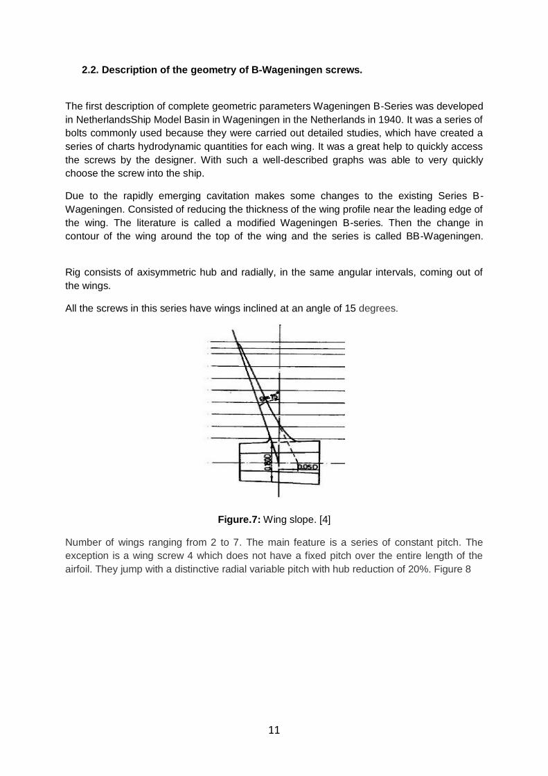
2.2. Description of the geometry of B-Wageningen screws.
The first description of complete geometric parameters Wageningen B-Series was developed
in NetherlandsShip Model Basin in Wageningen in the Netherlands in 1940. It was a series of
bolts commonly used because they were carried out detailed studies, which have created a
series of charts hydrodynamic quantities for each wing. It was a great help to quickly access
the screws by the designer. With such a well-described graphs was able to very quickly
choose the screw into the ship.
Due to the rapidly emerging cavitation makes some changes to the existing Series B-
Wageningen. Consisted of reducing the thickness of the wing profile near the leading edge of
the wing. The literature is called a modified Wageningen B-series. Then the change in
contour of the wing around the top of the wing and the series is called BB-Wageningen.
Rig consists of axisymmetric hub and radially, in the same angular intervals, coming out of
the wings.
All the screws in this series have wings inclined at an angle of 15 degrees.
Figure.7: Wing slope. [4]
Number of wings ranging from 2 to 7. The main feature is a series of constant pitch. The
exception is a wing screw 4 which does not have a fixed pitch over the entire length of the
airfoil. They jump with a distinctive radial variable pitch with hub reduction of 20%. Figure 8

12
Figure.8: Distribution pitch on the B-Wageningen screw. [2]
The most important features are parameterized geometric screw pitch coefficients, the coefficient of the surface of the upright and the number of wings. It is also important deflection profile, which affects the performance profile. The rest of the parameters are less important in driving characteristics. Parameters such as angle of attack, the airfoil contour profile are important in the phenomenon of cavitation. B-series has a small angle of the airfoil. Thus sound is cavitation properties. It's great if you do not need a special optimization for cavitation conditions.

13
Wing contour:
For 2 and 3 wings propeller table 1
For 4 to 7 wings propeller table 2.
r/R b/D*Z/(Ae/Ao) b1/b b0/b
0,2 1,633 0,616 0,35
0,3 1,832 0,611 0,35
0,4 2 0,599 0,35
0,5 2,12 0,583 0,355
0,6 2,186 0,558 0,389
0,7 2,168 0,526 0,442
0,8 2,027 0,481 0,478
0,9 1,657 0,4 0,5
1 0 0 0
Table 1.
r/R b/D*Z/(Ae/Ao) b1/b b0/b
0,2 1,662 0,617 0,35
0,3 1,882 0,613 0,35
0,4 2,05 0,601 0,351
0,5 2,152 0,586 0,355
0,6 2,187 0,561 0,389
0,7 2,144 0,524 0,443
0,8 1,97 0,463 0,479
0,9 1,582 0,351 0,5
1 0 0 0
Table 2.

14
b – chord length
b1 – distance from the axis of the leading edge of the wing
b0 – the distance from the leading edge of the Line of maximum thickness
D – diameter of the screw
Z – wings number
AE – screw upright surface area
AO – screw circle area
Maksymalne grubości profili zostały opisane współczynnikami w tabeli 3:
r/R tmax/D
2-skrzydła 3-skrzydła 4-skrzydła 5-skrzydeł 6-skrzydeł 7-skrzydeł
0.2 0.0406 0.0406 0.0366 0.0326 0.0286 0.0246
0.3 0.0359 0.0359 0.0324 0.0289 0.0254 0.0219
0.4 0.0312 0.0312 0.0282 0.0252 0.0222 0.0192
0.5 0.0265 0.0265 0.0240 0.0215 0.0190 0.0165
0.6 0.0218 0.0218 0.0198 0.0178 0.0158 0.0138
0.7 0.0171 0.0171 0.0156 0.0141 0.0126 0.0111
0.8 0.0124 0.0124 0.0114 0.0104 0.0094 0.0084
0.9 0.0077 0.0077 0.0072 0.0067 0.0062 0.0057
1.0 0.0030 0.0030 0.0030 0.0030 0.0030 0.0030
Table 3.
where,
tmax – wing thickness at a given radius.
Wings geometry profile:
Y coordinates of the contour profiles at different radius are meaning by formula:
For the contour points from the drailing edge to the Line of maximum thickness:
yc=V1(tmax-tte)
ys-yc=V2(tmax-tte)+tte
For the contour points from the Line of maximum thickness to the leading edge:
yc= V1(tmax-tle)
ys-yc=V2(tmax-tle)+tle

15
Figure. 9: Wings geometry profile.
where:
yc- pressure ordinate side of profile
ys- suction ordinate side of profile
tmax- maximum profile thickness
tte- trailing edge thickness
tle- leading edge thickness
V1- coefficient
V2- coefficient
ys-yc – local thickness of the profile measured perpendicular to the pitch
r/R – ratio of the distance of individual sections of the screw axis
Coefficient value V1
(r/R) -1 -0,8 -0,6 -0,4 -0,2 0 0,2 0,4 0,6 0,8 1
1 0 0 0 0 0 0 0 0 0 0 0
0,9 0 0 0 0 0 0 0 0 0 0 0
0,8 0 0 0 0 0 0 0 0 0 0 0
0,7 0 0 0 0 0 0 0 0 0 0 0
0,6 0 0 0 0 0 0 0 0 0 0,0006 0,0382
0,5 0,0522 0,019 0,004 0 0 0 0 0 0,0034 0,0211 0,1278
0,4 0,1467 0,063 0,0126 0,0044 0 0 0 0,0033 0,0189 0,0637 0,2181
0,3 0,2306 0,1333 0,0623 0,0202 0,0033 0 0,0027 0,0148 0,0503 0,1191 0,2923
0,2 0,2826 0,1967 0,1207 0,0592 0,0172 0 0,0049 0,0304 0,0804 0,1685 0,356

16
Table 4.
Coefficient value V1 from -1 to 0 are the values of the contour of the trailing edge to the line
of maximum thickness of the profile. From 0 to 1 are the values of the stroke than the
maximum thickness to the leading edge.
Coefficient value V2
(r/R) -1 -0,8 -0,6 -0,4 -0,2 0 0,2 0,4 0,6 0,8 1
1 0 0,36 0,64 0,84 0,96 1 0,96 0,84 0,64 0,36 0
0,9 0 0,36 0,64 0,84 0,96 1 0,96 0,84 0,64 0,36 0
0,8 0 0,36 0,64 0,84 0,96 1 0,9635 0,852 0,6545 0,3765 0
0,7 0 0,36 0,64 0,84 0,96 1 0,9675 0,866 0,684 0,414 0
0,6 0 0,3585 0,6415 0,8426 0,9613 1 0,969 0,879 0,72 0,462 0
0,5 0 0,3569 0,6439 0,8456 0,9639 1 0,971 0,888 0,7478 0,5039 0
0,4 0 0,35 0,6353 0,8415 0,9645 1 0,9725 0,8933 0,7593 0,522 0
0,3 0 0,336 0,6195 0,8265 0,9583 1 0,975 0,892 0,752 0,513 0
0,2 0 0,306 0,5842 0,7984 0,9446 1 0,975 0,8875 0,7277 0,4777 0
Table 5.
Coefficient value V2 from -1 to 0 are the values of the contour of the drailing edge to the Line
of maximum thickness of the profile. From 0 to 1 are the values of the stroke than the
maximum thickness to the leading edge.

17
Rys.10. Description of the trailing edge and leading edge.
Value tle and tte designer selects the tight local resistance of the propeller blade.
Recommended values for the initial calculation can be determined from table 6.
r/R tte/tmax tle/tmax
0.2 0.065562 0.1072
0.3 0.0775602 0.0968
0.4 0.1 0.0986
0.5 0.115 0.0994
0.6 0.12 0.0998
0.7 0.125 0.121
0.8 0.13 0.1335
0.9 0.142969 0.142969
Table 6.

18
2.3. Description of the properties of B-Wageningen screw.
The results of model tests are presented screws free charts usually called hydrodynamic
characteristics of the propeller.
The y-axis (ordinate) are dimensionless coefficients of the screw:
Coefficient of thrust
Coefficient moment
Coefficient of efficient
The x-axis
Advance ratio
Figure.11: Hydrodynamic charakcteristics of fixed screw. [2]

19
Where:
T – pressure [N]
ρ – water density [kg/m3]
Q – torque [Nm}
n – screw speed [Obr/s]
D – screw diameter [m]
VA – relative forward speed [m/s]
Modelling studies emerged some bolt group giving the best results in terms of performance
and efficiency. Maximum efficiency falls to a certain value of the load factor of stroke.
Propeller should be designed to work as long as possible in terms of the state. Variables
swimming conditions do not allow for continuous operation at maximum efficiency. Swimming
in the heavier conditions would decrease efficiency.
An important parameter that affects hydrodynamic characteristics is to change the pitch
position. Has the greatest influence on the change in the value of thrust force and torque
screws. With the increase in the value of the coefficient of stroke increases the pressure
coefficient and torque. With the increased stroke rate also increases the maximum efficiency
point of the screw. Maximum then shifts toward higher values of J. So screw has a high
efficiency, if it is a high rate of stroke, the relationship unfortunately works only to the
appropriate value of the feed. To the extreme point of the function η then decreases with
increasing feed rate.
Figure:12. Hydrodynamic characteristics of the screw. Extreme values of efficiency.
20
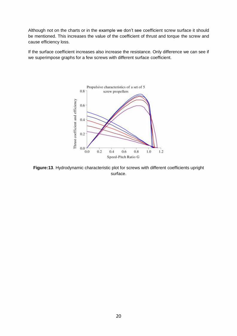
Although not on the charts or in the example we don’t see coefficient screw surface it should
be mentioned. This increases the value of the coefficient of thrust and torque the screw and
cause efficiency loss.
If the surface coefficient increases also increase the resistance. Only difference we can see if
we superimpose graphs for a few screws with different surface coefficient.
Figure:13. Hydrodynamic characteristic plot for screws with different coefficients upright
surface.

21
3. CFD simulation.
CFD, Computational Fluid Dynamics is a numerical fluid mechanic. This is a branch of fluid
mechanics that uses numerical methods for solving fluid flow problems.
With the numerical solution of partial differential equations describing the flow, we can
determine the approximate distribution of temperature, pressure, speed, etc. Recent CFD
programs allow to solve flows including viscosity and compressibility of multiphase flows,
flows in which there are chemical reactions and combustion processes and flows of
Newtonian fluid where we or non-Newtonian.
A large part of today's program is based on the Navier-Stokes equation which is the equation
of conservation of mass, momentum and energy of the fluid) and digitizes (the field is divided
into finite elements) them using the finite volume method, finite element or finite difference
methods.
4. Description of the process of creating parametric model 3D.
The basic requirement to perform my simulation is to have a 3D model that describes the
geometry of the propeller Wageningen B-series. My goal is to create a series of multi-
parametric model Wageningen B-screw to modify any of its geometrical characteristics.
In this way we obtain models of bolts of any diameter of the smallest diameter for boats
inland to the huge size of the bolts screws several meters in diameter. With some
variable is given the ability to create a variety of screws, e.g. by changing the pitch
uciągowej. We can influence the number of leaves and an upright surface ratio. The
finished model can be entered in the electronic version of 3D printers (small models) or
the machine number and receive the finished product. Here we will use only the model
for CFD simulation and verification of compliance charts hydrodynamic characteristics.
We create a parametric model screw-dependent of input variables:
Pitch coeffcient
Screw diameter
Wing number
Coefficient upright surface

22
4.1. Describing of model 3D
Parametric model based on the approximately 650 parameters and is dependent on four
variables. These variables are:
D – screw diameter
P/D – pitch coeffcient (in software called PD)
A – coefficient upright surface
z – wings number
Figure. 14: Table having variables manipulating the model.

23
Figure. 15: Profile created by polylines.
Begin to build a model by creating profiles on various levels described the ratio r / R
which is the radius of the beam cross-section of the screw. So in turn created profiles at
0.2, 0.3, etc. to 1.0. First of all, create the local coordinates of points defining the outline
of the profile. The coordinates are parameterized dependencies in model. Thanks for the
input data change automatically changes the profile of the wing.
Points combine function "spline" (a NURBS curve) and we formed the outline of the
profile.
Figure. 16: Profile tangent curve to spiral.

24
For each profile, we define a spiral, with a stroke of the screw, allowing for proper orientation
of the profile with respect to the axis.
Is tangent to the spiral plane on which a profile of the wing. We want our profile has changed
its tilt angle with the change of the spiral spring. It has a relationship exist between them. The
best solution is to create a line tangent to the spiral. The line must be on a plane where you
have created a profile to make it all made sense. The beginning of this line must be in the
intersection point between the plane and the spiral profile. Then create a line of acting at that
point, and also tangent to the spiral. We determine the relationship between the line parallel
to the axis of the helix and the local profile. Then, each time the helix pitch changes the angle
profile. Repeat operations for each profile.
Having already built the profile of the wing on the right pitch diameter cylinder creating a
spiral and a plane tangent to the (so-called tangent datum) Figure 17
Hub screw 2 and 3 - the wing has a coefficient of diameter D and the 0180*D 4 - 7 have a
diameter of 0.167*D.
Figure. 17: The plane tangent to the cylinder.

25
Figure. 18: The plane tangent to cylinder, second sketch.
Then coiled function „wrap” profile on the roller and we get a wings profile.
Figure. 19: Sketched onto the roller profile.

26
Repeat operations for each section until you get to r/R = 1.0.
Figure. 20: Effects work, sketches a few profiles.
The ends of profile sketches points in profiles like leading and trailing edges we sketch on
cylinders and join by spline function and we get the contour of wing.
Figure. 21: Preliminary profile of the wing.

27
Fill it surfaces constructed by using the "through curve". The result is a model of wing.
Figure. 22: The finished product. B-Wageningen screw model.
The flap we copy by function "instance geometry" around the hub. This is a feature that
allows us to quickly replicate any objects. We get a series of B-screw Wageningen.
Parameters describing the screw profiles differ between options for different numbers of
wings, so saved them in batches "2.txt", "3.txt", "4.txt", "5.txt", "6.txt" "7.txt "and can be
specified in one command.

28
Figure. 23: View of window with files for the model.
Simplifying the model:
Hub has been modeled as a shaft and end chamfering although normally in a series
of B-Wageningen appeared like an arc in the drawing selected No.1 line.
Figure.24: Simplifying the model:hub.
No rounding the leading and trailing edges of the wings. Are not included. B-series
models Wagenigen tested in the cavitation tunnel contained rounded edges, and the
lack of accurate data on how rounding them. That's why I decided not to create them
in the model.
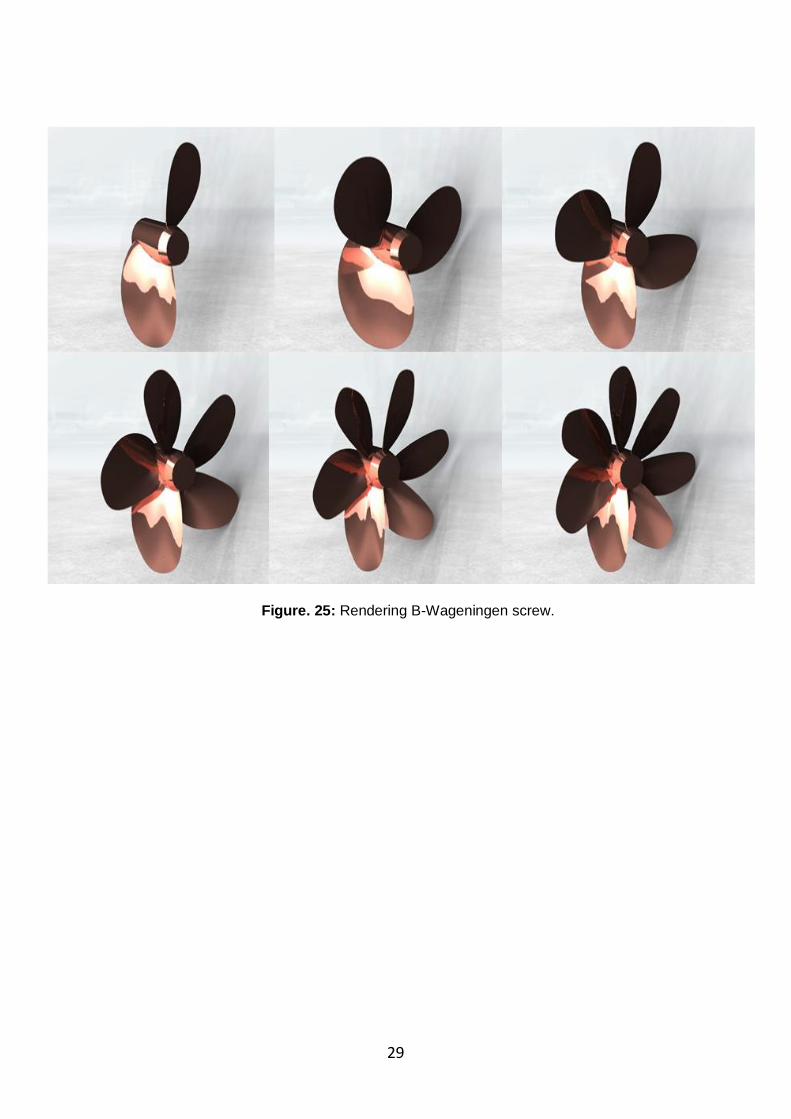
29
Figure. 25: Rendering B-Wageningen screw.

30
5. Describing CFD simulation.
Calculations were done in the STAR-CCM+. To create charts hydrodynamic characteristics
CFD simulations conducted nine screws for a series of three leaf surface with a coefficient of
0.50 upright. All calculations were performed in a standardized environment. Only the flow of
water to change to get the proper feed rate J at constant speeds 5 revolutions per second. 3
sets of calculations were obtained for three different values of pitch position (0.5, 0.8, 1.4).
Model has a screw diameter of 0.6 meters.
Figure. 26: View on propeller environment.
Screw is surrounded by water in the environment and more specifically in the cylinder of
water. Mesh was by the method of Finite Volume Method polyhedralmesher function. Our
net shapely form polyhedra (octahedron, dodecahedron)

31
Figure. 27:Water volume. Finite Volume Method. 1.093.692 cells.
Figure. 28: Grid computing on the surface of the screw.

32
Screw with the transmission shaft is disposed in the cylinder of water.
Cylinder diameter 3,5 m.
The distance from the inflow was 4 screws to the outlet is 2.1 m
Speed 5 revolutions per second.
Turbulence model: K-Epsilon
Water density 997,561 kg/m3
Dynamic viscosity 8,8871e-4
Grid computing Finite Volume Method: 1.093.692 cells.
Figure. 29: The properties are in the program describing simulation paramaters.
Figure. 30: The tab corresponding to the model grid.

33
We developed a bookmark or a description of the properties of the Continua, meshing model and
physical properties. We choose mesher polyhedral mesh method, because it is a better model than
Tetrahedral mesh. The difference is the geometry of the grid elements. Three-dimensional grid of
"Tetrahedral" consists of tetrahedra. However, grid-type "polyhedral" based on regular polyhedra
such as octahedron and dodecahedron giving greater accuracy, because it has more points, edges
and faces. In addition, polyhedral cells are less susceptible to stretching. Intelligent generation and
optimization techniques offer many possibilities grid: cells can automatically connect, share lib
modified by introducing additional points, edges, and faces. They also have a lower memory
requirement, increased computational speed and less number of iterations needed to obtain a result.
We have also added Prism Layer mesher, because we want to screw around patches of wall surfaces
were created. STAR-CCM+ asks you to input a number and the rest in an intelligent way he adjusts to
the calculation.
Figure. 31: Option in Reference Values.

34
Figure. 32: Option in physics properties.
The physical properties of the model:
Numerical soultions can be either implicit or explicit.
a) Implicit is a transient state when a solution is defined as a series of
interdependent equations or matrix dependent variables in an iterative way.
b) Exlicit it is clear the state where the simulation is described in more
interdependent equations giving the so-called clear solution. identity.
Likewise, we can choose whether the model is to be unsteady or shaky or Steady or
constant.
a) Model Steady in each iteration will be resolved first continuous flow lines are then
calculated from the current state of the specified initial conditions input and output
stream of water..
b) Model unsteady is that the fluid particles trajectories are calculated step by step
by step after each specified time, the particle will have a new position. At each
step, a new iteration is created between a continuous flow of particles. Each
iteration contains a certain amount of DPM or Discrete Phase Model or
poditeracji.
Select the method of Implicit unsteady.

35
Turbulence model types in STAR-CCM+:
a) K-Epsilon Turbulence is the most common model of turbulence. Turbulence
model comprises two equations which are solved for the turbulent kinetic energy
and its dissipation rate. The program has seven different models of K-Epsilon.
b) K-Omega Turbulence also has two equations and is alternative for K-Epsilon.
Plus over the previous model is the improved perfomance of boundary layers in
adverse pressure gradient. Minus by which is less used than the k-epsilon model
is that the calculation boundary layer is very sensitive to flow freely, and there are
problems with the inlet.
c) Reynolds Stress Turbulance (RST) some of the most complex models of
turbulence. They are used to calculate the model, where the quick-change and
the strain rate for simulation, where there is a secondary flow in the channels.
d) Spalart-Almaras Turbulence (SAT) consists of only one equation. It occurs in the
aerospace industry because of the ease of calculation. Unfortunately, our
calculations have checked up.
For the calculations we model K-Epsilon because of the good modeling of the boundary
layer, which under the influence of the inlet stream is not disrupted. It is very versatile and
does not need a model for the extended RST or SAT tests because they are too simple
to model these phenomena air will not be satisfied with us.

36
Figure. 33: In the physical properties of the initial flow rate set.
The physical properties we set the initial data such as inlet pressure, the type of
turbulence and velocity. Last given what will be our crucial because only it will change.
We will give the speed in m / s with a negative sign, so we have created since the frame
of reference.
.

37
Figure. 34: Defininig elements in program.
In the "Region 1" have placed our body that is defined elements such as screw shaft wall environment, the inlet and outlet of the cylinder.
Figure. 35: Solvers type we use.
Solvers tab from which we will use computational methods.
Figure. 36: Plots.

38
Plots serves us to obtain the graph of the results of the simulation.
Figure. 37: By this function arises screw rotation.
In the title Motions we set number of turns screws environment. In a simulation, it does not
screw rotate but the environment revolves around the water only environment around the
propeller. With a speed of 5 revolutions per second.
Research propeller description:
Propeller diameter 0.6 m
We have got three different screw pitch
For each stroke rate fall three calculations for three different feed rates to achieve
hydrodynamic characteristics charts
Studies enviromental is everywhere the same
In any calculation of the flow velocity changes of water flow due to the normalized
number of turns to get the proper feed rates.
Name description:
B – this is series of B-Wageningen screw
B_3 – 3 wings
B_3_50 – coefficient upright surface is 0.50
B_3_50_pitch50 – pitch coefficient equal 0.50
B_3_50_pitch50_015 – feed coefficient is 0.15

39
First simulation B_3_50_pitch50_015:
1) Absolute pressure
2) Pressure

40
3) Moments plot obtained by three wings.
4) Force plot obtained by three wings.

41
Second simulation B_3_50_pitch50_020:
1) Absolute pressure
2) Pressure

42
3) Moments plot obtained by three wings.
4) Force plot obtained by three wings.

43
Third simulation B_3_50_pitch50_030:
1) Absolute pressure
2) Pressure

44
3) Moment plot obtained by three wings.
4) Force plot obtained by three wings.

45
Fourth simulation B_3_50_pitch80_030:
1) Absolute pressure
2) Pressure
46
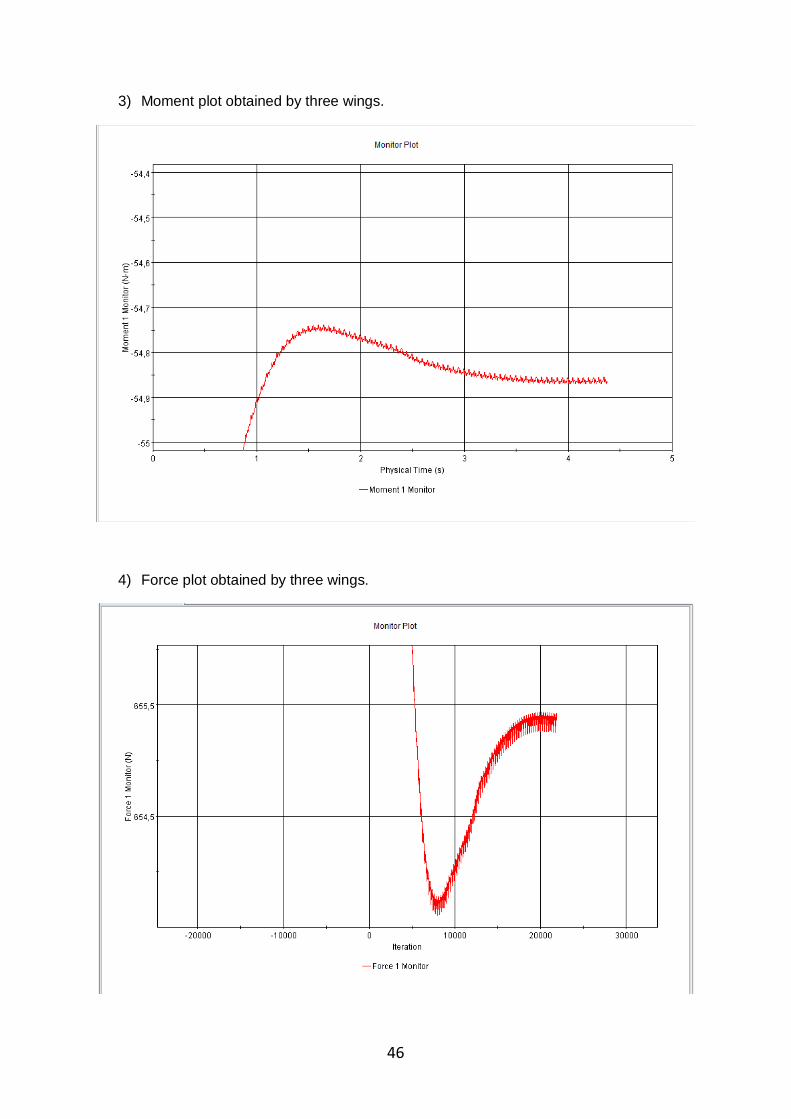
3) Moment plot obtained by three wings.
4) Force plot obtained by three wings.

47
Fifth simulation B_3_50_pitch80_045:
1) Absolute pressure
2) Pressure

48
3) Moment plot obtained by three wings.
4) Force plot obtained by three wings.

49
Six simulation B_3_50_pitch80_060:
1) Absolute pressure
2) Pressure

50
3) Moment plot obtained by three wings.
4) Force plot obtained by three wings.

51
Seventh simulation B_3_50_pitch140_060:
1) Absolute pressure
2) Pressure
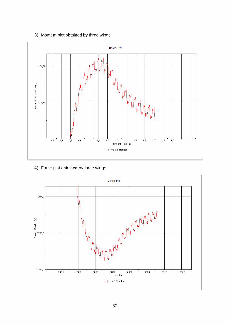
52
3) Moment plot obtained by three wings.
4) Force plot obtained by three wings.

53
Eighth simulation B_3_50_pitch140_080:
1) Absolute pressure
2) Pressure

54
3) Moment plot obtained by three wings.
4) Force plot obtained by three wings.

55
Ninth simulation B_3_50_pitch140_110:
1) Absolute pressure
2) Pressure

56
3) Moment plot obtained by three wings.
4) Force plot obtained by three wings.
57
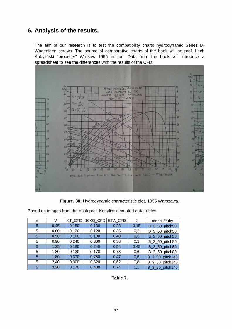
6. Analysis of the results.
The aim of our research is to test the compatibility charts hydrodynamic Series B-
Wagenigen screws. The source of comparative charts of the book will be prof. Lech
Kobyliński "propeller" Warsaw 1955 edition. Data from the book will introduce a
spreadsheet to see the differences with the results of the CFD.
Figure. 38: Hydrodynamic characteristic plot, 1955 Warszawa.
Based on images from the book prof. Kobylinski created data tables.
n V KT_CFD 10KQ_CFD ETA_CFD J model śruby
5 0,45 0,150 0,130 0,28 0,15 B_3_50_pitch50
5 0,60 0,130 0,120 0,35 0,2 B_3_50_pitch50
5 0,90 0,100 0,100 0,48 0,3 B_3_50_pitch50
5 0,90 0,240 0,300 0,38 0,3 B_3_50_pitch80
5 1,35 0,180 0,240 0,54 0,45 B_3_50_pitch80
5 1,80 0,130 0,170 0,73 0,6 B_3_50_pitch80
5 1,80 0,370 0,750 0,47 0,6 B_3_50_pitch140
5 2,40 0,300 0,620 0,62 0,8 B_3_50_pitch140
5 3,30 0,170 0,400 0,74 1,1 B_3_50_pitch140
Table 7.

58
where:
n – propeller rotation speed [rot/s]
V – inlet water velocity [m/s]
KT_CFD – coefficient KT[-]
10KQ_CFD – coeffcient KQ [-]
ETA_CFD – propeller effciency [-]
J – feed coeffcient
Variable in our calculations is the feed rate is thanks to him we generate flow velocity.
The data that we obtained from studies in STAR-CCM+ from CD-Adapco are listed
below:
n V T Q KT_CFD 10KQ_CFD ETA_CFD J model śruby
5 0,45 304,50 20,80 0,094 0,107 0,21 0,15 B_3_50_pitch50
5 0,60 259,80 18,84 0,080 0,097 0,26 0,2 B_3_50_pitch50
5 0,90 158,92 14,40 0,049 0,074 0,32 0,3 B_3_50_pitch50
5 0,90 655,00 54,85 0,203 0,283 0,34 0,3 B_3_50_pitch80
5 1,35 462,85 41,32 0,143 0,213 0,48 0,45 B_3_50_pitch80
5 1,80 258,50 26,85 0,080 0,138 0,55 0,6 B_3_50_pitch80
5 1,80 1263,60 174,83 0,391 0,901 0,41 0,6 B_3_50_pitch140
5 2,40 975,15 138,84 0,302 0,716 0,54 0,8 B_3_50_pitch140
5 3,30 534,20 83,68 0,165 0,431 0,67 1,1 B_3_50_pitch140
Table 8.
where:
T – Force on three wings [N]
Q – Moment on three wings [Nm]
The graphs below are the presentation of the results of the charts hydrodynamic read from
the book "propeller" marked by "TK" or cavitation tunnel. The graphs are the values resulting
from CFD simulation models for each end of the bolt and have a "CFD".

59
Figure.39: Hydrodynamic characteristic plot for screw B_3_50 with pitch coefficient 0.50.
Comparison of CFD results and cavitation tunnel (CT)
Measuring differences: B_3_50_pitch50
KT [%] KQ [%] n [%]
J=0.15 37,2 17,5 23,9
J=0.20 38,2 19,1 23,6
J=0.30 50,9 25,8 33,8
Rys.40: Hydrodynamic characteristic plot for screw B_3_50 with pitch coefficient 0.80.
Comparison of CFD results and cavitation tunnel (CT)

60
Measuring difference: B_3_50_pitch80
KT [%] KQ [%] n [%]
J=0.30 15,6 5,8 10,4
J=0.45 20,5 11,3 10,4
J=0.60 38,5 18,6 24,5
Rys.41: Hydrodynamic characteristic plot for screw B_3_50 with pitch coefficient 1.40.
Comparison of CFD results and cavitation tunel (CT)
Measuring difference: B_3_50_pitch140
% KT [%] KQ [%] n [%]
J=0.60 -5,6 -20,2 12,1
J=0.80 -0,5 -15,4 12,9
J=1.10 2,8 -7,8 9,9
There is a big difference between the closest matching measurements to reach 0.5% in
the model B_3_50_pitch140 B_3_50_pitch50 to 50.9%. The data that we obtained from
CFD calculations for bolts and B_3_50_pitch80 B_3_50_pitch50 are always below the
charts of the cavitation tunnel. However, for the screw marked KT B_3_50_pitch140
characteristics obtained from CFD simulation is the characteristics of the cavitation tunnel
and efficiency graphs intersect.
After the tests, the CFD model did not obtain satisfactory characteristics compliance with
the graphs of the results obtained from the book Prof. Kobylinski "Śruby okrętowe".
Potential sources of differences:
a) other provisions adopted in the simulation during the test (temperature, pressure,
viscosity of water)
b) errors in the preparation of the data (simulation conditions, simplified geometry,
coarse mesh)
c) errors in the selection of computational models
d) software error

61
Figure. 42: Drawing of the edge of the propeller blade. The simplified geometry.
Figure. 43: Stress concentration AT the leading edge.
In Figure 43 showing strongly reduced pressure in the center of wings. The reason causing
the phenomenon may be to simplify the modeling of edge or screw geometry error. I think
that may be the flow separation at the leading edge and the formation of turbulent flow.

62
The big problem in CFD simulation was problem that we didn’t know conditions in the
cavitation tunnel tests contained in the book prof. Lech Kobylinski. That's why I decided to
use the default value of ambient water for STAR-CCM+: water density and viscosity 997.561
kg/m3 8.8871 e-4 Pa / s
To test the effect of temperature, I make addtional simualtion on the screw B_3_50_pitch50.
T Q KT_CFD 10KQ_CFD ETA_CFD J water temp. density viscosity
310,58 21,15 0,096 0,109 0,21 0,15 about 25 degree 997,561 0,00088871
304,50 20,80 0,094 0,107 0,21 0,15 23 degree 998,29 0,00100300
Tabela 9.
Value was previously used for the water temperature around 25 degrees. After checking the
temperature effect on the calculations say that it has a big impact. For such small
temperature changes of up two degrees difference in the calculation of coefficients KT and
KQ is 2%. In summary it has a great impact on the results of the CFD. If the tunnel was a
different temperature, pressure and salinity than those established in this numerical
difference can be very large.
7. Analysis of the results.
The results do not support the thesis clearly staked, showing differences from the
experimental results. However, keep in mind that even in the case of measurements made at
different times and in different centers, there are differences in the results achieved [3]. The
problem requires further examination, however, it is outside the scope of engineering work. It
would also be interesting to examine the compatibility of the results obtained using different
programs.
The simulations do not cover the full range of variability mainly due to the long-term
calculations and the need to reduce the execution time of a diploma. Full, systematic studies
are carried out by research centers and go far beyond the scope of engineering work.
The fact that he could not confirm the compatibility of the results with the results of the
simulation model does not prove erroneous method. The results may be the result of errors
made in the preparation and implementation of the simulation.
Very important is a thorough knowledge of all the conditions of the study. It turns out that
even a well documented series of research, it is fully described in terms of the study, which
introduces significant uncertainty in the process.

63
8. Bibliography
[1] Carlton John „Marine Propellers and Propulsion”, 2007 Second Edition
[2] Dudziak J. „Teoria okrętu”, 2008 Gdańsk
[3] Kobyliński L. „Śruby okrętowe”, 1955 Warszawa
[4] The Wageningen Propeller Series
[5] Wanot J. opracowanie “Geometria śrub serii B i BB Wageningen”
Related Documents


