Parameterized Machine Learning for High-Energy Physics · Parameterized Machine Learning for High-Energy Physics ... more parameters that describe the larger scope of the ... 4 3

Parameterized Machine Learning for High-Energy Physics

Pierre Baldi,1 Kyle Cranmer,2 Taylor Faucett,3 Peter Sadowski,1 and Daniel Whiteson3

1Department of Computer Science, University of California, Irvine, CA 926972Department of Physics, NYU, New York, NY

3Department of Physics and Astronomy, University of California, Irvine, CA 92697(Dated: February 1, 2016)

We investigate a new structure for machine learning classifiers applied to problems in high-energyphysics by expanding the inputs to include not only measured features but also physics parameters.The physics parameters represent a smoothly varying learning task, and the resulting parameterizedclassifier can smoothly interpolate between them and replace sets of classifiers trained at individualvalues. This simplifies the training process and gives improved performance at intermediate values,even for complex problems requiring deep learning. Applications include tools parameterized interms of theoretical model parameters, such as the mass of a particle, which allow for a singlenetwork to provide improved discrimination across a range of masses. This concept is simple toimplement and allows for optimized interpolatable results.

PACS numbers:

INTRODUCTION

Neural networks have been applied to a wide variety ofproblems in high-energy physics [1, 2], from event classi-fication [3, 4] to object reconstruction [5, 6] and trigger-ing [7, 8]. Typically, however, these networks are appliedto solve a specific isolated problem, even when this prob-lem is part of a set of closely related problems. An il-lustrative example is the signal-background classificationproblem for a particle with a range of possible masses.The classification tasks at different masses are related,but distinct. Current approaches require the training ofa set of isolated networks [9, 10], each of which are igno-rant of the larger context and lack the ability to smoothlyinterpolate, or the use of a single signal sample in train-ing [11, 12], sacrificing performance at other values.

In this paper, we describe the application of the ideasin Ref. [13] to a new neural network strategy, a param-eterized neural network in which a single network tack-les the full set of related tasks. This is done by simplyextending the list of input features to include not onlythe traditional set of event-level features but also one ormore parameters that describe the larger scope of theproblem such as a new particle’s mass. The approachcan be applied to any classification algorithm; however,neural networks provide a smooth interpolation, whiletree-based methods may not.

A single parameterized network can replace a set ofindividual networks trained for specific cases, as wellas smoothly interpolate to cases where it has not beentrained. In the case of a search for a hypothetical newparticle, this greatly simplifies the task – by requiringonly one network – as well as making the results morepowerful – by allowing them to be interpolated betweenspecific values. In addition, they may outperform iso-lated networks by generalizing from the full parameter-

dependent dataset.In the following, we describe the network structure

needed to apply a single parameterized network to a setof smoothly related problems and demonstrate the ap-plication for theoretical model parameters (such as newparticle masses) in a set of examples of increasing com-plexity.

NETWORK STRUCTURE & TRAINING

A typical network takes as input a vector of features,x̄, where the features are based on event-level quantities.After training, the resulting network is then a functionof these features, f(x̄). In the case that the task at handis part of a larger context, described by one or more pa-rameters, θ̄. It is straightforward to construct a networkthat uses both sets of inputs, x̄ and θ̄, and operates as afunction of both: f(x̄, θ̄). For a given set of inputs x̄0, atraditional network evaluates to a real number f(x̄0). Aparameterized network, however, provides a result that isparameterized in terms of θ̄: f(x̄0, θ̄), yielding differentoutput values for different choices of the parameters θ̄;see Fig. 1.

Training data for the parameterized network has theform (x̄, θ̄, y)i, where y is a label for the target class.The addition of θ̄ introduces additional considerationsin the training procedure. While traditionally the train-ing only requires the conditional distribution of x̄ givenθ̄ (which is predicted by the theory and detector sim-ulation), now the training data has some implicit priordistribution over θ̄ as well (which is arbitrary). When thenetwork is used in practice it will be to predict y condi-tional on both x̄ and θ̄, so the distribution of θ̄ used fortraining is only relevant in how it affects the quality ofthe resulting parameterized network – it does not imply

arX

iv:1

601.

0791

3v1

[he

p-ex

] 2

8 Ja

n 20

16

2

x1x2

fa(x1,x2)

θ=θa

x1x2

f(x1,x2,θ)

θ

x1x2

fb(x1,x2)

θ=θb

FIG. 1: Left, individual networks with input features(x1, x2), each trained with examples with a single value ofsome parameter θ = θa, θb. The individual networks arepurely functions of the input features. Performance for in-termediate values of θ is not optimal nor does it necessarilyvary smoothly between the networks. Right, a single networktrained with input features (x1, x2) as well as an input pa-rameter θ; such a network is trained with examples at severalvalues of the parameter θ.

that the resulting inference is Bayesian. In the studiespresented below, we simply use equal sized samples fora few discrete values of θ̄. Another issue is that some orall of the components of θ̄ may not be meaningful for aparticular target class. For instance, the mass of a newparticle is not meaningful for the background trainingexamples. In what follows, we randomly assign values tothose components of θ̄ according to the same distribu-tion used for the signal class. In the examples studiedbelow the networks have enough generalization capacityand the training sets are large enough that the resultingparameterized classifier performs well without any tuningof the training procedure. However, the robustness of theresulting parameterized classifier to the implicit distribu-tion of θ̄ in the training sample will in general depend onthe generalization capacity of the classifier, the numberof training examples, the physics encoded in the distribu-tions p(x̄|θ̄, y), and how much those distributions changewith θ̄.

TOY EXAMPLE

As a demonstration for a simple toy problem, we con-struct a parameterized network, which has a single in-put feature x and a single parameter θ. The networkis trained using labeled examples where examples withlabel 0 are drawn from a uniform background and exam-ples with label 1 are drawn from a Gaussian with meanθ and width σ = 0.25. Training samples are generatedwith θ = −2,−1, 0, 1, 2; see Fig. 2a.

As shown in Fig. 2, this network generalizes the so-lution and provides reasonable output even for valuesof the parameter where it was given no examples. Notethat the response function has the same shape for thesevalues (θ = −1.5,−0.5, 0.5, 1.5) as for values where train-ing data was provided, indicating that the network has

4 3 2 1 0 1 2 3 4x

0

1000

2000

3000

4000

5000

6000

7000

Num

ber

of

events/0.1

00x

θ=-2.0θ=-1.0θ=0.0θ=1.0θ=2.0

4 3 2 1 0 1 2 3 4input

0.0

0.2

0.4

0.6

0.8

1.0

NN

outp

ut

θ=−1.0

θ=−0.5

θ=0

θ=0.5

θ=1.0

TrainedInterpolated

FIG. 2: Top, training samples in which the signal is drawnfrom a Gaussian and the background is uniform. Bottom,neural network response as a function of the value of the inputfeature x, for various choices of the input parameter θ; notethat the single parameterized network has seen no trainingexamples for θ = −1.5,−0.5, 0.5, 1.5.

successfully parameterized the solution. The signal-background classification accuracy is as good for valueswhere training data exist as it is for values where trainingdata does not.

1D PHYSICAL EXAMPLE

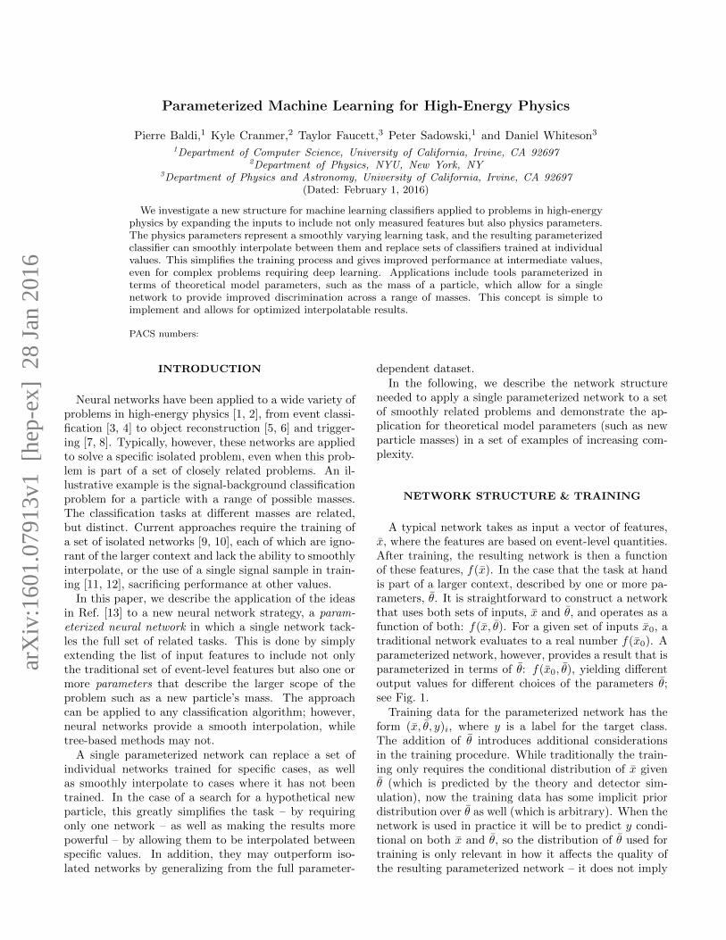
A natural physical case is the application to the searchfor new particle of unknown mass. As an example, weconsider the search for a new particle X which decaysto tt̄. We treat the most powerful decay mode, in whichtt̄ → W+bW−b̄ → qq′b`νb̄. The dominant backgroundis standard model tt̄ production, which is identical infinal state but distinct in kinematics due to the lack ofan intermediate resonance. Figure 3 shows diagrams forboth the signal and background processes.

We first explore the performance in a one-dimensionalcase. The single event-level feature of the network ismWWbb, the reconstructed resonance mass, calculatedusing standard techniques identical to those describedin Ref. [14]. Specifically, we assume resolved top quarksin each case, for simplicity. Events are are simulated atparton level with madgraph5 [15], using pythia [16]for showering and hadronization and delphes [17] with

3

t

t̄

W+ ℓ+

νq

q′

b̄

bq

q̄

X

W−

g

g

t

t̄

W+ ℓ+

νq

q′

b̄

b

W−

FIG. 3: Feynman diagrams showing the production and de-cay of the hypothetical particle X → tt̄, as well as the dom-inant standard model background process of top quark pairproduction. In both cases, the tt̄ pair decay to a single chargedlepton (`), a neutrino (ν) and several quarks (q, b).

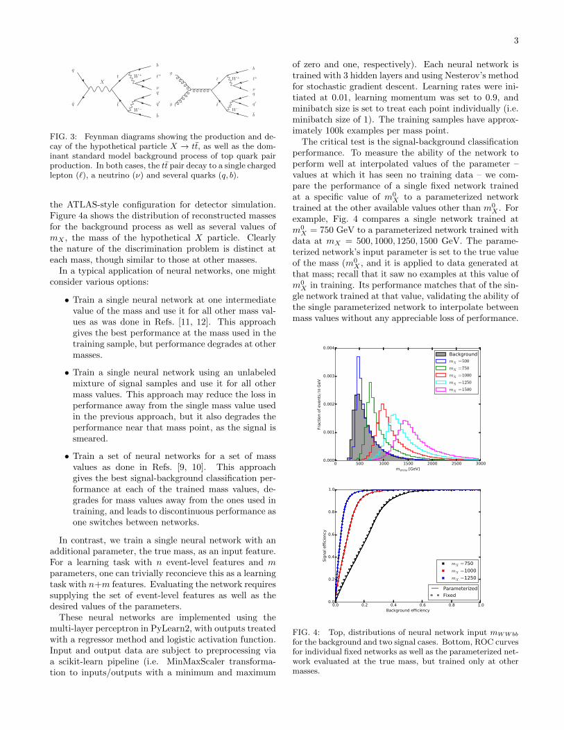
the ATLAS-style configuration for detector simulation.Figure 4a shows the distribution of reconstructed massesfor the background process as well as several values ofmX , the mass of the hypothetical X particle. Clearlythe nature of the discrimination problem is distinct ateach mass, though similar to those at other masses.

In a typical application of neural networks, one mightconsider various options:

• Train a single neural network at one intermediatevalue of the mass and use it for all other mass val-ues as was done in Refs. [11, 12]. This approachgives the best performance at the mass used in thetraining sample, but performance degrades at othermasses.

• Train a single neural network using an unlabeledmixture of signal samples and use it for all othermass values. This approach may reduce the loss inperformance away from the single mass value usedin the previous approach, but it also degrades theperformance near that mass point, as the signal issmeared.

• Train a set of neural networks for a set of massvalues as done in Refs. [9, 10]. This approachgives the best signal-background classification per-formance at each of the trained mass values, de-grades for mass values away from the ones used intraining, and leads to discontinuous performance asone switches between networks.

In contrast, we train a single neural network with anadditional parameter, the true mass, as an input feature.For a learning task with n event-level features and mparameters, one can trivially reconcieve this as a learningtask with n+m features. Evaluating the network requiressupplying the set of event-level features as well as thedesired values of the parameters.

These neural networks are implemented using themulti-layer perceptron in PyLearn2, with outputs treatedwith a regressor method and logistic activation function.Input and output data are subject to preprocessing viaa scikit-learn pipeline (i.e. MinMaxScaler transforma-tion to inputs/outputs with a minimum and maximum

of zero and one, respectively). Each neural network istrained with 3 hidden layers and using Nesterov’s methodfor stochastic gradient descent. Learning rates were ini-tiated at 0.01, learning momentum was set to 0.9, andminibatch size is set to treat each point individually (i.e.minibatch size of 1). The training samples have approx-imately 100k examples per mass point.

The critical test is the signal-background classificationperformance. To measure the ability of the network toperform well at interpolated values of the parameter –values at which it has seen no training data – we com-pare the performance of a single fixed network trainedat a specific value of m0

X to a parameterized networktrained at the other available values other than m0

X . Forexample, Fig. 4 compares a single network trained atm0X = 750 GeV to a parameterized network trained with

data at mX = 500, 1000, 1250, 1500 GeV. The parame-terized network’s input parameter is set to the true valueof the mass (m0

X , and it is applied to data generated atthat mass; recall that it saw no examples at this value ofm0X in training. Its performance matches that of the sin-

gle network trained at that value, validating the ability ofthe single parameterized network to interpolate betweenmass values without any appreciable loss of performance.

0 500 1000 1500 2000 2500 3000mWWbb [GeV]

0.000

0.001

0.002

0.003

0.004

Fract

ion o

f events/5

0 G

eV

BackgroundmX =500

mX =750

mX =1000

mX =1250

mX =1500

0.0 0.2 0.4 0.6 0.8 1.0Background efficiency

0.0

0.2

0.4

0.6

0.8

1.0

Sig

nal eff

icie

ncy

mX =750

mX =1000

mX =1250

ParameterizedFixed

FIG. 4: Top, distributions of neural network input mWWbb

for the background and two signal cases. Bottom, ROC curvesfor individual fixed networks as well as the parameterized net-work evaluated at the true mass, but trained only at othermasses.

4

HIGH-DIMENSIONAL PHYSICAL EXAMPLE

The preceding examples serve to demonstrate the con-cept in one-dimensional cases where the variation of theoutput on both the parameters and features can be eas-ily visualized. In this section, we demonstrate that theparameterization of the problem and the interpolationpower that it provides can be achieved also in high-dimensional cases.

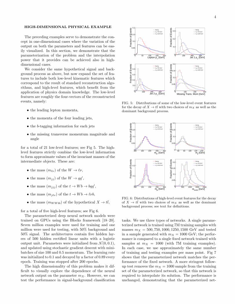
We consider the same hypothetical signal and back-ground process as above, but now expand the set of fea-tures to include both low-level kinematic features whichcorrespond to the result of standard reconstruction algo-rithms, and high-level features, which benefit from theapplication of physics domain knowledge. The low-levelfeatures are roughly the four-vectors of the reconstructedevents, namely:

• the leading lepton momenta,

• the momenta of the four leading jets,

• the b-tagging information for each jets

• the missing transverse momentum magnitude andangle

for a total of 21 low-level features; see Fig 5. The high-level features strictly combine the low-level informationto form approximate values of the invariant masses of theintermediate objects. These are:

• the mass (m`ν) of the W → `ν,

• the mass (mjj) of the W → qq′,

• the mass (mjjj) of the t→Wb→ bqq′,

• the mass (mj`ν) of the t→Wb→ `νb,

• the mass (mWWbb) of the hypothetical X → tt̄,

for a total of five high-level features; see Fig 6.The parameterized deep neural network models were

trained on GPUs using the Blocks framework [18–20].Seven million examples were used for training and onemillion were used for testing, with 50% background and50% signal. The architectures contain five hidden lay-ers of 500 hidden rectified linear units with a logisticoutput unit. Parameters were initialized from N (0, 0.1),and updated using stochastic gradient descent with mini-batches of size 100 and 0.5 momentum. The learning ratewas initialized to 0.1 and decayed by a factor of 0.89 everyepoch. Training was stopped after 200 epochs.

The high dimensionality of this problem makes it dif-ficult to visually explore the dependence of the neuralnetwork output on the parameter mX . However, we cantest the performance in signal-background classification

[GeV]T

Lepton p0 50 100 150 200

Fra

ctio

n of

Eve

nts

0

0.05

0.1

0.15

0.2Backg.

=750 GeVXm

=1250 GeVXm

[GeV]T

Jet 1 p0 200 400 600

Fra

ctio

n of

Eve

nts

0

0.1

0.2

0.3Backg.

=750 GeVXm

=1250 GeVXm

[GeV]T

Jet 2 p0 200 400 600

Fra

ctio

n of

Eve

nts

0

0.1

0.2

0.3

0.4

Backg.

=750 GeVXm

=1250 GeVXm

Missing Trans. Mom [GeV]0 100 200 300

Fra

ctio

n of

Eve

nts

0

0.05

0.1

0.15

0.2Backg.

=750 GeVXm

=1250 GeVXm

FIG. 5: Distributions of some of the low-level event featuresfor the decay of X → tt̄ with two choices of mX as well as thedominant background process.

[GeV]νjlm100 150 200 250 300

Fra

ctio

n of

Eve

nts

0

0.05

0.1

0.15

0.2Backg.

=750 GeVXm

=1250 GeVXm

[GeV]jjm60 80 100 120 140

Fra

ctio

n of

Eve

nts

0

0.05

0.1

0.15

0.2Backg.

=750 GeVXm

=1250 GeVXm

[GeV]jjjm100 150 200 250 300

Fra

ctio

n of

Eve

nts

0

0.1

0.2

Backg.

=750 GeVXm

=1250 GeVXm

[GeV]wwbbm0 500 1000 1500 2000

Fra

ctio

n of

Eve

nts

0

0.05

0.1

0.15

0.2Backg.

=750 GeVXm

=1250 GeVXm

FIG. 6: Distributions of high-level event features for the decayof X → tt̄ with two choices of mX as well as the dominantbackground process; see text for definitions.

tasks. We use three types of networks. A single parame-terized network is trained using 7M training samples withmasses mX = 500, 750, 1000, 1250, 1500 GeV and testedin a sample generated with mX = 1000 GeV; the perfor-mance is compared to a single fixed network trained withsamples at mX = 1000 (with 7M training examples).In each case, we use approximately the same numberof training and testing examples per mass point. Fig 7shows that the parameterized network matches the per-formance of the fixed network. A more stringent follow-up test removes the mX = 1000 sample from the trainingset of the parameterized network, so that this network isrequired to interpolate its solution. The performance isunchanged, demonstrating that the parameterized net-

5

0.0 0.2 0.4 0.6 0.8 1.0

Background efficiency

0.0

0.2

0.4

0.6

0.8

1.0

Sig

nal eff

icie

ncy

Parameterized NN

Parameterized NN (no data at 1000)

Network trained on all masses

Network trained at mass=1000 only

FIG. 7: Comparison of the signal-to-background discrimi-nation for four classes of networks for a testing sample withmX = 1000 GeV. A parameterized network trained on a setof masses (mX = 500, 750, 1000, 1250, 1500) is compared to asingle network trained at mX = 1000 GeV. The performanceis equivalent. A second parameterized network is trained onlywith samples at mx = 500, 750, 1250, 1500, forcing it to in-terpolate the solution at mX = 1000 GeV. Lastly, a singlenon-parameterized network trained with all the mass pointsshows a reduced performance. The results are indistinguish-able for cases where the networks use only low-level features(shown) or low-level as well as high-level features (not shown,but identical).

work is capable of generalizing the solution even in ahigh-dimensional example.

Conversely, Fig 8 compares the performance of theparameterized network to a single network trained atmX = 1000 GeV when applied across the mass rangeof interest, which is a common application case. Thisdemonstrates the loss of performance incurred by tradi-tional approaches and recovered in this approach. Simi-larly, we see that a single network trained an unlabeledmixture of signal samples from all masses has reducedperformance at each mass value tested.

In previous work, we have shown that deep networkssuch as these do not require the additional of high-levelfeatures [21, 22] but are capable of learning the necessaryfunctions directly from the low-level four-vectors. Herewe extend that by repeating the study above withoutthe use of the high-level features; see Fig 7. Using onlythe low-level features, the parameterized deep networkis achieves essentially indistinguishable performance forthis particular problem and training sets of this size.

DISCUSSION

We have presented a novel structure for neural net-works that allows for a simplified and more powerful so-lution to a common use case in high-energy physics anddemonstrated improved performance in a set of exam-ples with increasing dimensionality for the input featurespace. While these example use a single parameter θ, the

500 750 1000 1250 1500

Mass of signal

0.5

0.6

0.7

0.8

0.9

1.0

AU

C

Parameterized NN (mass is a feature)

Network trained on all masses

Network trained at mass=1000 only

FIG. 8: Comparison of the performance in the signal-background discrimination for the parameterized network,which learns the entire problem as a function of mass, and asingle network trained only at mX = 1000 GeV. As expected,the AUC score decreases for the single network as the massdeviates from the value in the training sample. The param-eterized network shows improvement over this performance;the trend of improving AUC versus mass reflects the increas-ing separation between the signal and background sampleswith mass, see Figs. 5 and 6. For comparison, also shown inthe performance a single network trained with an unlabeledmixture of signal samples at all masses.

technique is easily applied to higher dimensional param-eter spaces.

Parameterized networks can also provide optimizedperformance as a function of nuisance parameters thatdescribe systematic uncertainties, where typical networksare optimal only for a single specific value used duringtraining. This allows statistical procedures that makeuse of profile likelihood ratio tests [23] to select the net-work corresponding to the profiled values of the nuisanceparameters [13].

Datasets used in this paper containing millions ofsimulated collisions can be found in the UCI MachineLearning Repository [24] at archive.ics.uci.edu/ml/

datasets/HEPMASS.

Acknowledgements

We thank Tobias Golling, Daniel Guest, Kevin Lan-non, Juan Rojo, Gilles Louppe, and Chase Shimminfor useful discussions. KC is supported by the US Na-tional Science Foundation grants PHY-0955626, PHY-1205376, and ACI-1450310. KC is grateful to UC-Irvinefor their hospitality while this research was initiated andthe Moore and Sloan foundations for their generous sup-port of the data science environment at NYU. We thankYuzo Kanomata for computing support. We also wish toacknowledge a hardware grant from NVIDIA, NSF grantIIS-1550705, and a Google Faculty Research award toPB.

6

[1] Bruce H. Denby. Neural Networks and Cellular Au-tomata in Experimental High-energy Physics. Comput.Phys. Commun., 49:429–448, 1988.

[2] Carsten Peterson, Thorsteinn Rognvaldsson, and LeifLonnblad. JETNET 3.0: A Versatile artificial neuralnetwork package. Comput. Phys. Commun., 81:185–220,1994.

[3] P. Abreu et al. Classification of the hadronic decays ofthe Z0 into b and c quark pairs using a neural network.Phys. Lett., B295:383–395, 1992.

[4] Hermann Kolanoski. Application of artificial neural net-works in particle physics. Nucl. Instrum. Meth., A367:14–20, 1995.

[5] Carsten Peterson. Track Finding With Neural Networks.Nucl. Instrum. Meth., A279:537, 1989.

[6] Georges Aad et al. A neural network clustering algorithmfor the ATLAS silicon pixel detector. JINST, 9:P09009,2014.

[7] Leif Lonnblad, Carsten Peterson, and Thorsteinn Rogn-valdsson. Finding Gluon Jets With a Neural Trigger.Phys. Rev. Lett., 65:1321–1324, 1990.

[8] Bruce H. Denby, M. Campbell, Franco Bedeschi,N. Chriss, C. Bowers, and F. Nesti. Neural Networks forTriggering. IEEE Trans. Nucl. Sci., 37:248–254, 1990.

[9] T. Aaltonen et al. Evidence for a particle produced inassociation with weak bosons and decaying to a bottom-antibottom quark pair in Higgs boson searches at theTevatron. Phys. Rev. Lett., 109:071804, 2012.

[10] Serguei Chatrchyan et al. Combined results of searchesfor the standard model Higgs boson in pp collisions at√s = 7 TeV. Phys. Lett., B710:26–48, 2012.

[11] Georges Aad et al. Search for W ′ → tb̄ in the lepton plusjets final state in proton-proton collisions at a centre-of-mass energy of

√s = 8 TeV with the ATLAS detector.

Phys. Lett., B743:235–255, 2015.[12] Serguei Chatrchyan et al. Search for Z ’ resonances de-

caying to tt̄ in dilepton+jets final states in pp collisionsat√s = 7 TeV. Phys. Rev., D87(7):072002, 2013.

[13] Kyle Cranmer. Approximating Likelihood Ratios withCalibrated Discriminative Classifiers. 2015.

[14] Georges Aad et al. Search for a multi-Higgs-boson cas-cade in W+Wbb̄ events with the ATLAS detector in ppcollisions at

√s = 8TeV. Phys. Rev., D89(3):032002,

2014.[15] Johan Alwall, Michel Herquet, Fabio Maltoni, Olivier

Mattelaer, and Tim Stelzer. MadGraph 5 : Going Be-yond. JHEP, 1106:128, 2011.

[16] Torbjorn Sjostrand, Stephen Mrenna, and Peter Z.Skands. PYTHIA 6.4 Physics and Manual. JHEP,0605:026, 2006.

[17] J. de Favereau et al. DELPHES 3, A modular frame-work for fast simulation of a generic collider experiment.JHEP, 1402:057, 2014.

[18] Bart van Merrinboer, Dzmitry Bahdanau, Vincent Du-moulin, Dmitriy Serdyuk, David Warde-Farley, JanChorowski, and Yoshua Bengio. Blocks and Fuel: Frame-works for deep learning. arXiv:1506.00619 [cs, stat], June2015. arXiv: 1506.00619.

[19] Frdric Bastien, Pascal Lamblin, Razvan Pascanu, JamesBergstra, Ian J. Goodfellow, Arnaud Bergeron, NicolasBouchard, and Yoshua Bengio. Theano: new features and

speed improvements. 2012. Published: Deep Learningand Unsupervised Feature Learning NIPS 2012 Work-shop.

[20] James Bergstra, Olivier Breuleux, Frdric Bastien, Pas-cal Lamblin, Razvan Pascanu, Guillaume Desjardins,Joseph Turian, David Warde-Farley, and Yoshua Bengio.Theano: a CPU and GPU Math Expression Compiler.In Proceedings of the Python for Scientific ComputingConference (SciPy), Austin, TX, June 2010. Oral Pre-sentation.

[21] Pierre Baldi, Peter Sadowski, and Daniel Whiteson.Searching for Exotic Particles in High-Energy Physicswith Deep Learning. Nature Commun., 5:4308, 2014.

[22] Pierre Baldi, Peter Sadowski, and Daniel Whiteson. En-hanced Higgs Boson to τ+τ− Search with Deep Learning.Phys. Rev. Lett., 114(11):111801, 2015.

[23] Glen Cowan, Kyle Cranmer, Eilam Gross, and OferVitells. Asymptotic formulae for likelihood-based testsof new physics. Eur. Phys. J., C71:1554, 2011.

[24] Pierre Baldi, Kyle Cranmer, Taylor Faucett, Pe-ter Sadowski, and Daniel Whiteson. UCI machinelearning repository. http://archive.ics.uci.edu/ml/

datasets/HEPMASS, 2015.