Parameterization-free Projection for Geometry …lipmanya/lop/LOP_final_TR.pdfParameterization-free Projection for Geometry Reconstruction Yaron Lipman Daniel Cohen-Or David Levin

Parameterization-free Projection for Geometry ReconstructionYaron Lipman Daniel Cohen-Or David Levin

Tel-Aviv UniversityHillel Tal-Ezer

Academic Collegeof Tel-Aviv Yaffo

Abstract

We introduce a Locally Optimal Projection operator (LOP) forsurface approximation from point-set data. The operator is parame-terization free, in the sense that it does not rely on estimating a localnormal, fitting a local plane, or using any other local parametricrepresentation. Therefore, it can deal with noisy data which cluttersthe orientation of the points. The method performs well in casesof ambiguous orientation, e.g., if two folds of a surface lie neareach other, and other cases of complex geometry in which methodsbased upon local plane fitting may fail. Although defined by aglobal minimization problem, the method is effectively local, and itprovides a second order approximation to smooth surfaces. Henceallowing good surface approximation without using any explicit orimplicit approximation space. Furthermore, we show that LOP ishighly robust to noise and outliers and demonstrate its effectivenessby applying it to raw scanned data of complex shapes.

Keywords: point-cloud, surface reconstruction, geometry,projection operator

1 Introduction

Reconstructing the geometry of a shape from scanned data has beenan important research objective in the last two decades [Hoppeet al. 1992; Amenta et al. 1998; Levoy et al. 2000; Kazhdan et al.2006]. Despite the proliferation of surface reconstruction tech-niques, many aspects of the problem remain open. Two prominentdifficulties in the reconstruction process are shape complexity andnoise. Surface reconstruction methods (e.g., [Hoppe et al. 1992;Alexa et al. 2001; Carr et al. 2001; Ohtake et al. 2003; Amentaand Kil 2004; Kazhdan et al. 2006]) work well when the data isdensely sampled and the orientation of the points can be deducedfrom the samples themselves. In the case of complex geometry(e.g., Figure 1) the surface cannot be reasonably approximated bya simple oriented manifold, that is, it cannot be well parameterizedand approximated over a local plane. Such a scenario, for example,is manifested in thin parts where two folds of the shape are closeto each other and the noise level is high. Therefore, augmentingthe data points with orientation, either by supplying normals oroff-surface points, is an extremely hard task.

Reconstruction by a projection operator has an important virtue:It defines a consistent geometry based on the data points, andprovides constructive means to up-sample it. For example, theMLS projection operator [Levin 2003] has been established as apowerful surface reconstruction technique. However, the MLS

(a)

(b)

(b)

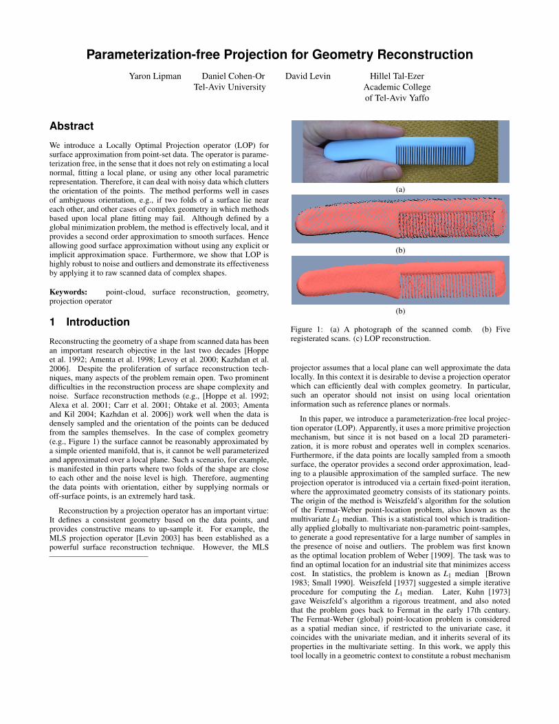
Figure 1: (a) A photograph of the scanned comb. (b) Fiveregisterated scans. (c) LOP reconstruction.

projector assumes that a local plane can well approximate the datalocally. In this context it is desirable to devise a projection operatorwhich can efficiently deal with complex geometry. In particular,such an operator should not insist on using local orientationinformation such as reference planes or normals.

In this paper, we introduce a parameterization-free local projec-tion operator (LOP). Apparently, it uses a more primitive projectionmechanism, but since it is not based on a local 2D parameteri-zation, it is more robust and operates well in complex scenarios.Furthermore, if the data points are locally sampled from a smoothsurface, the operator provides a second order approximation, lead-ing to a plausible approximation of the sampled surface. The newprojection operator is introduced via a certain fixed-point iteration,where the approximated geometry consists of its stationary points.The origin of the method is Weiszfeld’s algorithm for the solutionof the Fermat-Weber point-location problem, also known as themultivariate L1 median. This is a statistical tool which is tradition-ally applied globally to multivariate non-parametric point-samples,to generate a good representative for a large number of samples inthe presence of noise and outliers. The problem was first knownas the optimal location problem of Weber [1909]. The task was tofind an optimal location for an industrial site that minimizes accesscost. In statistics, the problem is known as L1 median [Brown1983; Small 1990]. Weiszfeld [1937] suggested a simple iterativeprocedure for computing the L1 median. Later, Kuhn [1973]gave Weiszfeld’s algorithm a rigorous treatment, and also notedthat the problem goes back to Fermat in the early 17th century.The Fermat-Weber (global) point-location problem is consideredas a spatial median since, if restricted to the univariate case, itcoincides with the univariate median, and it inherits several of itsproperties in the multivariate setting. In this work, we apply thistool locally in a geometric context to constitute a robust mechanism

(a) (b) (c) (d) (e) (f)

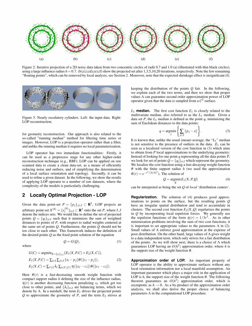
Figure 2: Iterative projection of a 2D noisy data taken from two concentric circles of radii 0.7 and 1.0 (a) (illustrated with thin black circles),using a large influence radius h = 0.7. (b),(c),(d),(e),(f) show the projected set after 1,3,5,10,20 iterations, respectively. Note the few remaining“floating points”, which can be removed by local analysis, see Section 2. Moreover, note that the expected shrinkage effect is insignificant (f).

Figure 3: Nearly osculatory cylinders. Left: the input data. Right:LOP reconstruction.

for geometry reconstruction. Our approach is also related to theso-called ”running median” method for filtering time series orimages. However, LOP is a projection operator rather than a filter,and unlike the running median it requires no local parameterization.

LOP operator has two immediate functionalities: Firstly, itcan be used as a preprocess stage for any other higher-orderreconstruction technique (e.g., RBF). LOP can be applied on rawscanned data to create a clean data-set, as a means of efficientlyreducing noise and outliers, and of simplifying the determinationof a local surface orientation and topology. Secondly, it can beused to refine a given dataset. In the following, we show the resultsof applying LOP operator to a number of raw datasets, where thecomplexity of the models is particularly challenging.

2 Locally Optimal Projection - LOP

Given the data point-set P = {p j} j∈J ⊂ R3, LOP projects an

arbitrary point-set X (0) = {x(0)i }i∈I ⊂ R3 onto the set P, where I,J

denote the indices sets. We would like to define the set of projectedpoints Q = {qi}i∈I such that it minimizes the sum of weighteddistances to points of P, with respect to radial weights centered atthe same set of points Q. Furthermore, the points Q should not betoo close to each other. This framework induces the definition ofthe desired points Q as the fixed point solution of the equation

Q = G(Q), (1)where

G(C) = argminX={xi}i∈I{E1(X ,P,C)+E2(X ,C)},

E1(X ,P,C) = ∑i∈I ∑ j∈J ‖xi− p j‖θ(‖ci− p j‖),

E2(X ,C) = ∑i′∈I λi′ ∑i∈I\{i′}η(‖xi′ − ci‖)θ(‖ci′ − ci‖).

(2)

Here θ(r) is a fast-decreasing smooth weight function withcompact support radius h defining the size of the influence radius,η(r) is another decreasing function penalizing xi′ which get tooclose to other points, and {λi}i∈I are balancing terms, which wedenote by Λ. In a nutshell, the term E1 drives the projected pointsQ to approximate the geometry of P, and the term E2 strives at

keeping the distribution of the points Q fair. In the following,we explain each of the two terms, and then we show that propervalues Λ can guarantee second order approximation power of LOPoperator given that the data is sampled from a C2 surface.

L1 median. The first cost function E1 is closely related to themultivariate median, also referred to as the L1 median. Given adata set P, the L1 median is defined as the point q, minimizing thesum of Euclidean distances to the data points:

q = argminx

{∑j∈J‖p j − x‖

}. (3)

It is known that, unlike the usual (mean) average, the “L1” medianis not sensitive to the presence of outliers in the data. E1 can beseen as a localized version of the cost function in (3) which aimsto obtain from P local approximations to the underlying geometry:Instead of looking for one point q representing all the data points P,we look for set of points Q = {qi}i∈I which represent the geometry.We localize the cost function using a fast-decaying weight functionθ with the finite support radius h (we used the approximationθ(r) = e−r2/(h/4)2

). The solution ofQ = argmin

XE1(X ,P,Q) (4)

can be interpreted as being the set Q of local ‘distribution centers’.

Regularization. The solution of (4) produces good approx-imations to points on the surface, but the resulting points Qhave an irregular spatial distribution and tend to accumulate inclusters. The second cost function E2(X ,Q) regularizes the pointsin Q by incorporating local repulsion forces. We generally usethe repulsion functions of the form η(r) = 1/3r3. As in otherminimization problems involving the sum of two cost functions, itis important to set appropriate values to the parameters Λ in (2).Small values of Λ enforce good approximation at the expense ofpoor distribution. On the other hand, large values of Λ gives weightto a data independent term, which only strives for a fair distributionof the points. As we will show next, there is a choice of Λ whichguarantees LOP having an O(h2) approximation order, where h isthe support size of the weight function θ .

Approximation order of LOP. An important property ofLOP operator is the ability to approximate surfaces without anylocal orientation information nor a local manifold assumption. Animportant parameter which plays a major role in the application ofLOP is h, the support size of the weight function θ . The followingtheorem guarantees an O(h2) approximation order, which isasymptotic as h → 0. As a by-product of the approximation orderanalysis, we shall also derive the proper choice of balancingparameters Λ in the computational LOP procedure.

Theorem 2.1. If the data set P is sampled from a C2-smoothsurface S, LOP operator has an O(h2) approximation order to S ,provided that Λ is carefully chosen.

Proof. In letting h tend to zero we assume that thenumber of projected points, I, is fixed, while the num-ber of input points, J, may grow. G(C), as defined in(2), satisfies ∇X |X=G(C) (E1(X ,P,C)+E2(X ,C)) = 0. There-fore, the points Q = {qi}i∈I defined by Eq. (1) satisfying∇X |X=Q (E1(X ,P,Q)+E2(X ,Q)) = 0, which leads to the relation:

∑j∈J

(qi′ − p j)α i′j −λi′ ∑

i∈I\{i′}(qi′ −qi)β i′

i = 0 , i′ ∈ I, (5)

where α i′j = θ(‖qi′−p j‖)

‖qi′−p j‖ , j ∈ J and β i′i = θ(‖qi′−qi‖)

‖qi′−qi‖

∣∣∣ ∂η(‖qi′−qi‖)∂ r

∣∣∣,i ∈ I \ {i′}. Note that we have used the fact that η is decreasing,that is, its derivative is always negative. After rearranging and

setting λi′ = µ∑ j∈J α i′

j

∑i∈I\{i′} β i′i

, µ > 0, we get

(1−µ)qi′ +µ ∑i∈I\{i′}

qiβ i′

i

∑i∈I\{i′} β i′i

= ∑j∈J

p jα i′

j

∑ j∈J α i′j

, i′ ∈ I. (6)

Viewing (6) as a system of equations for Q,

AQ = R, (7)

Note that both A and R are also depending on Q, yet, by analyzingA−1 and R we show below that Q = A−1R are points at distanceO(h2) from the surface S. The proof is by showing that each qi′ is anaverage of nearby points, on the surface or near it. We shall use theobservation that an affine average of points on a plane is also on thatplane, and that the surface can be locally approximated by a plane,with an approximation error of O(h2). The sum on the r.h.s. of (6)represents a local convex combination of points within a distance hfrom qi′ . We may assume that this sum is not empty. Otherwise, by(6) it follows that qi′ is at, or near, the origin, and such points willbe discarded. Thus, using the local plane reconstruction property ofaffine combinations, we have that the r.h.s. equals F +O(h2), whereF = { fi′}i′∈I are points on S. Also, due to the finite support of θ , wefurther have | fi−qi| ≤ h+O(h2). Next, we have AQ = F +O(h2).If we take µ ∈ [0,1/2), then A is strictly diagonally dominantand therefore we can bound ‖A−1‖∞ ≤ 1

1−µ ∑∞k=0(

µ

1−µ)k = 1

1−2µ.

Now, since the rows of A sum up to one, so do the rows ofA−1. Furthermore, we note that |(A−1)`,m| ≤ a1(

µ

1−µ)k when the

distance between q` and qm is greater or equal to kh; that is, theinfluence of distant points decays exponentially with distance.The above implies that Q = A−1F + O(h2), and each element(A−1F)i′ is an affine average of fi on the surface, with weightsexponentially decaying with the distance ‖ fi′ − fi‖. Let T bethe tangent plane to S at fi′ , and let fi = ti + ri where ti is theprojection of fi on T . It can be shown that ‖ri‖ < a2‖ fi − fi′‖2.Then (A−1F)i′ = ∑i∈I A−1

i′,i (ti + ri) = ∑i∈I A−1i′,i ti + ∑i∈I A−1

i′,i ri.

We would first like to show that ‖∑i∈I A−1i′,i ti − fi′‖ = O(h)

and since ∑i∈I A−1i′,i ti is on T it will follow that it is an O(h2)

distant from S. Secondly, we will show ∑i∈I A−1i′,i ri = O(h2).

This will show that (A−1F)i′ and consequently qi′ is O(h2)distant from S. Then, for a fixed i′ let us denote by Ik theset of indices of points qi such that ‖qi − qi′‖ ∈ [kh,(k + 1)h).∥∥∥∑i∈I A−1

i′,i ti− fi′∥∥∥ =

∥∥∥∑i∈I A−1i′,i (ti− fi′)

∥∥∥≤∑k≥0 ∑i∈Ik

a1(µ

1−µ)k ((k +1)h+O(h)) = O(h). (8)

Next, in the same way, using the observation that‖ri‖ < a2((k + 1)h + O(h))2, for i ∈ Ik, we conclude that‖∑i∈I A−1

i′,i ri‖= O(h2).

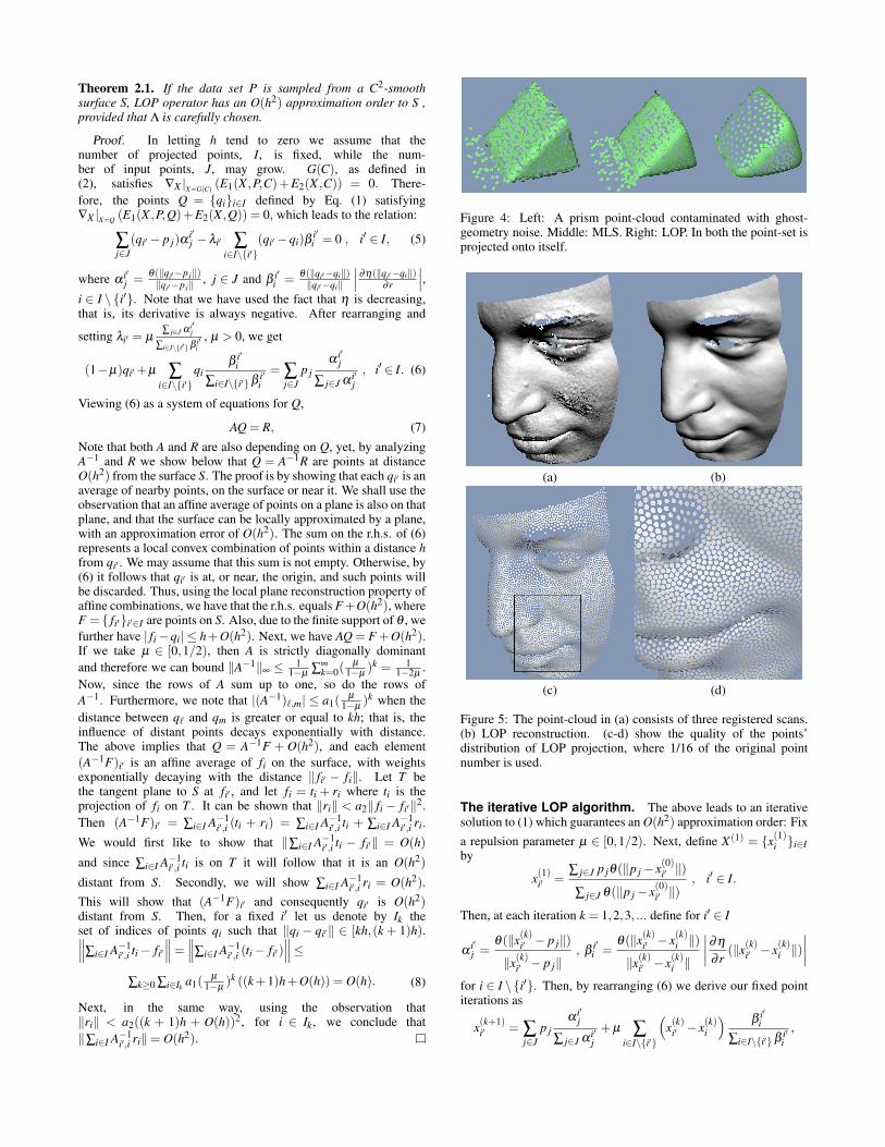
Figure 4: Left: A prism point-cloud contaminated with ghost-geometry noise. Middle: MLS. Right: LOP. In both the point-set isprojected onto itself.

(a) (b)

(c) (d)

Figure 5: The point-cloud in (a) consists of three registered scans.(b) LOP reconstruction. (c-d) show the quality of the points’distribution of LOP projection, where 1/16 of the original pointnumber is used.

The iterative LOP algorithm. The above leads to an iterativesolution to (1) which guarantees an O(h2) approximation order: Fixa repulsion parameter µ ∈ [0,1/2). Next, define X (1) = {x(1)

i }i∈Iby

x(1)i′ =

∑ j∈J p jθ(‖p j − x(0)i′ ‖)

∑ j∈J θ(‖p j − x(0)i′ ‖)

, i′ ∈ I.

Then, at each iteration k = 1,2,3, ... define for i′ ∈ I

αi′j =

θ(‖x(k)i′ − p j‖)

‖x(k)i′ − p j‖

, βi′i =

θ(‖x(k)i′ − x(k)

i ‖)

‖x(k)i′ − x(k)

i ‖

∣∣∣∣∂η

∂ r(‖x(k)

i′ − x(k)i ‖)

∣∣∣∣for i ∈ I \ {i′}. Then, by rearranging (6) we derive our fixed pointiterations as

x(k+1)i′ = ∑

j∈Jp j

α i′j

∑ j∈J α i′j

+ µ ∑i∈I\{i′}

(x(k)

i′ − x(k)i

)β i′

i

∑i∈I\{i′} β i′i

,

for every i′ ∈ I. Upon convergence, the limit satisfies the necessarycondition (5), and by Theorem 2.1 the approximation order isguaranteed. Figure 2 exhibits a 2D example of the iterative process.There could be a small number of points which LOP operatormight not project as expected. There are two typical scenarios:(i) The point’s distance from the surface is larger than the supportsize of the influence weight function θ , that is h. (ii) The point isexactly midway between two attractors; for example, see Figure 2(f). In both cases these problematic points can easily be detectedvia a local points’ distribution analysis, since the weighted densityin the vicinity of such points is smaller than the density of thepoints on the surface. In our implementation we detect these pointsusing a parameter and discard them.

(a) (b) (c) (d)

Figure 6: Up-sample/down-sample example. A planar point-cloud(a) was projected onto itself using LOP (b). (c) shows projectionof a halved set onto the original data (a) (down-sample). (d) showsprojection of doubled set (up-sample).

Application of LOP. LOP can be used to project an arbitraryset of points X (0) onto an input point-cloud P. We observe that tak-ing X (0) with less points than P results in more regular distributionof projected points, see Figure 6 and 5(c–d). The rationale is thatthe input data can be regarded as consisting of multiple observationof the same data (e.g., multiple registered scans), and LOP operatorgenerates a concise set of points that represents well the input data.In a sense, it operates like a multivariate median, which defines arepresentative to a set of samples. Then, to up-sample the initialprojection, we enriched the above projected set and performed few(≈ 3 or 4) iterations of LOP. It is important to note that LOP israther independent of the initial guess X (0). See Figure 8 where aninitial crude guess results in a fair and faithful approximation. LOPalgorithm is controlled by two parameters: h and µ . To study theirinfluence on the properties of the projected set Q, see Figure 12. his the local influence size of the operator; it is usually best to startthe iterations with h as large as the expected outliers magnitudeand then refine h as the iterations progress. Similarly, one can startwith a small µ and then increase it. µ reflects the tradeoff betweenaccuracy (µ ∈ [0.1,0.25]) and regular distribution (µ ∈ [0.3,0.45]).

3 Results and conclusions

Figures 1, 5, 7, 10 show the results of applying LOP to rawdata-sets acquired by a scanner. For each model a number of scansare registered, forming a noisy and incomplete point-cloud. Theshape of the models that we use are challenging. Figure 3 showsa synthetic example where the correct topology of two near oscu-latory cylinders is reconstructed by LOP. Figures 4, 9, 10 and 11show different comparisons of LOP and MLS. All the examples arerendered using PointShop3D [Zwicker et al. 2002]. The normalsused for shading are computed with the same local PCA algorithm.In Figure 10 we used voxel data extracted from multi-view video.

The algorithm requires typically 20 iterations of averaging forprojecting a point-set onto itself. An exception is the exampledepicted in Figure 8, where the initial guess X (0) is very crude,

(a) (b) (c)

(d) (e) (f)

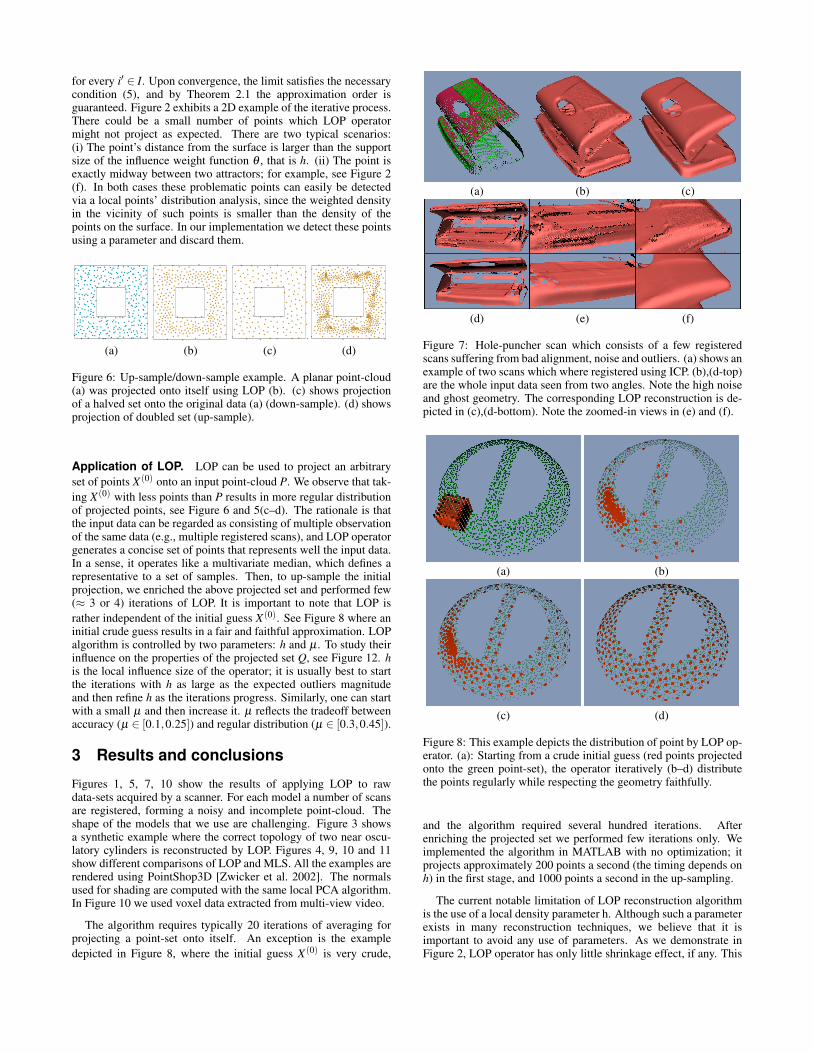
Figure 7: Hole-puncher scan which consists of a few registeredscans suffering from bad alignment, noise and outliers. (a) shows anexample of two scans which where registered using ICP. (b),(d-top)are the whole input data seen from two angles. Note the high noiseand ghost geometry. The corresponding LOP reconstruction is de-picted in (c),(d-bottom). Note the zoomed-in views in (e) and (f).

(a) (b)

(c) (d)

Figure 8: This example depicts the distribution of point by LOP op-erator. (a): Starting from a crude initial guess (red points projectedonto the green point-set), the operator iteratively (b–d) distributethe points regularly while respecting the geometry faithfully.

and the algorithm required several hundred iterations. Afterenriching the projected set we performed few iterations only. Weimplemented the algorithm in MATLAB with no optimization; itprojects approximately 200 points a second (the timing depends onh) in the first stage, and 1000 points a second in the up-sampling.

The current notable limitation of LOP reconstruction algorithmis the use of a local density parameter h. Although such a parameterexists in many reconstruction techniques, we believe that it isimportant to avoid any use of parameters. As we demonstrate inFigure 2, LOP operator has only little shrinkage effect, if any. This

(a) (b)

(c) (d)

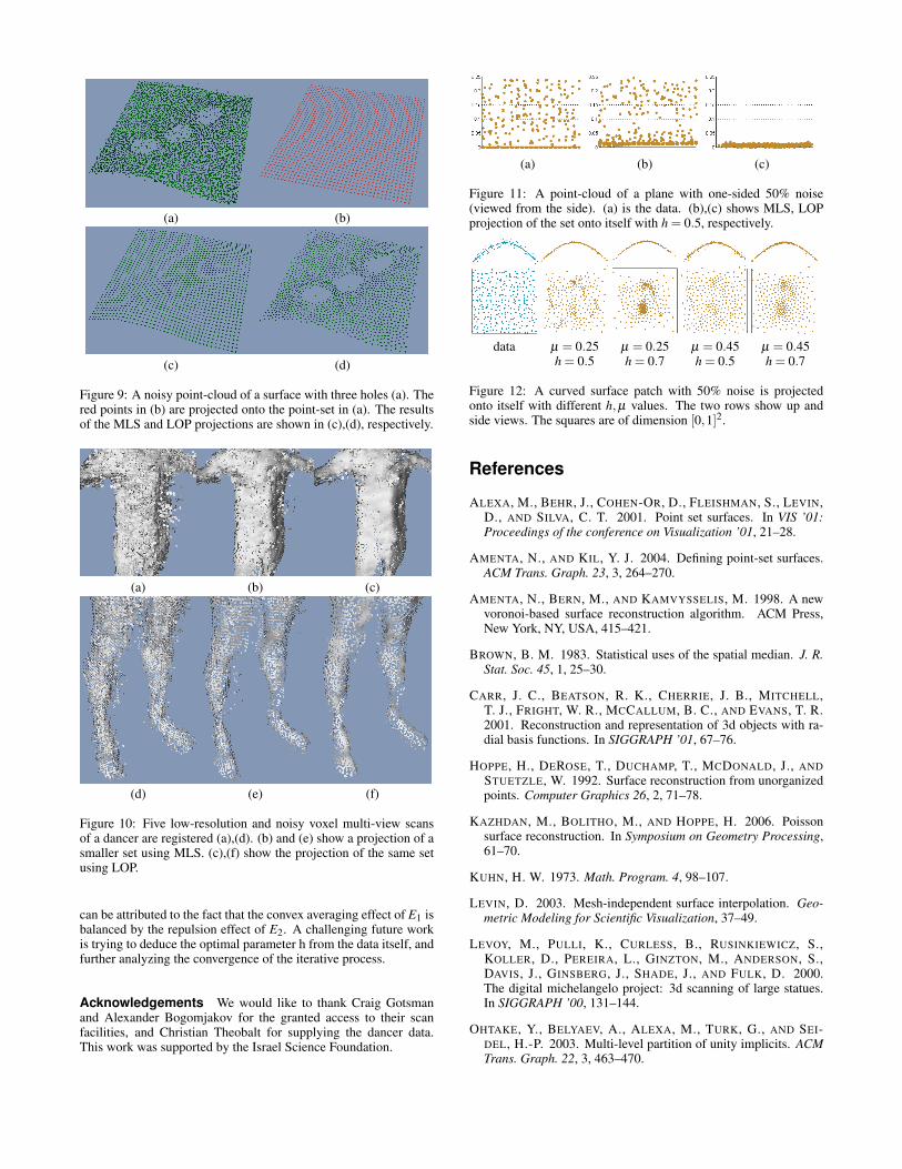
Figure 9: A noisy point-cloud of a surface with three holes (a). Thered points in (b) are projected onto the point-set in (a). The resultsof the MLS and LOP projections are shown in (c),(d), respectively.

(a) (b) (c)

(d) (e) (f)

Figure 10: Five low-resolution and noisy voxel multi-view scansof a dancer are registered (a),(d). (b) and (e) show a projection of asmaller set using MLS. (c),(f) show the projection of the same setusing LOP.

can be attributed to the fact that the convex averaging effect of E1 isbalanced by the repulsion effect of E2. A challenging future workis trying to deduce the optimal parameter h from the data itself, andfurther analyzing the convergence of the iterative process.

Acknowledgements We would like to thank Craig Gotsmanand Alexander Bogomjakov for the granted access to their scanfacilities, and Christian Theobalt for supplying the dancer data.This work was supported by the Israel Science Foundation.

(a) (b) (c)

Figure 11: A point-cloud of a plane with one-sided 50% noise(viewed from the side). (a) is the data. (b),(c) shows MLS, LOPprojection of the set onto itself with h = 0.5, respectively.

data µ = 0.25 µ = 0.25 µ = 0.45 µ = 0.45h = 0.5 h = 0.7 h = 0.5 h = 0.7

Figure 12: A curved surface patch with 50% noise is projectedonto itself with different h,µ values. The two rows show up andside views. The squares are of dimension [0,1]2.

References

ALEXA, M., BEHR, J., COHEN-OR, D., FLEISHMAN, S., LEVIN,D., AND SILVA, C. T. 2001. Point set surfaces. In VIS ’01:Proceedings of the conference on Visualization ’01, 21–28.

AMENTA, N., AND KIL, Y. J. 2004. Defining point-set surfaces.ACM Trans. Graph. 23, 3, 264–270.

AMENTA, N., BERN, M., AND KAMVYSSELIS, M. 1998. A newvoronoi-based surface reconstruction algorithm. ACM Press,New York, NY, USA, 415–421.

BROWN, B. M. 1983. Statistical uses of the spatial median. J. R.Stat. Soc. 45, 1, 25–30.

CARR, J. C., BEATSON, R. K., CHERRIE, J. B., MITCHELL,T. J., FRIGHT, W. R., MCCALLUM, B. C., AND EVANS, T. R.2001. Reconstruction and representation of 3d objects with ra-dial basis functions. In SIGGRAPH ’01, 67–76.

HOPPE, H., DEROSE, T., DUCHAMP, T., MCDONALD, J., ANDSTUETZLE, W. 1992. Surface reconstruction from unorganizedpoints. Computer Graphics 26, 2, 71–78.

KAZHDAN, M., BOLITHO, M., AND HOPPE, H. 2006. Poissonsurface reconstruction. In Symposium on Geometry Processing,61–70.

KUHN, H. W. 1973. Math. Program. 4, 98–107.

LEVIN, D. 2003. Mesh-independent surface interpolation. Geo-metric Modeling for Scientific Visualization, 37–49.

LEVOY, M., PULLI, K., CURLESS, B., RUSINKIEWICZ, S.,KOLLER, D., PEREIRA, L., GINZTON, M., ANDERSON, S.,DAVIS, J., GINSBERG, J., SHADE, J., AND FULK, D. 2000.The digital michelangelo project: 3d scanning of large statues.In SIGGRAPH ’00, 131–144.

OHTAKE, Y., BELYAEV, A., ALEXA, M., TURK, G., AND SEI-DEL, H.-P. 2003. Multi-level partition of unity implicits. ACMTrans. Graph. 22, 3, 463–470.

SMALL, C. G. 1990. A survey of multidimensional medians. Int.Stat. rev. 58, 3, 263–277.

WEBER, A. 1909. [translated by Carl J. Friedrich from Weber’s1909 book]. Theory of the Location of Industries. Chicago: TheUniversity of Chicago Press, 1929.

WEISZFELD, E. 1937. Sur le point pour lequel la somme desdistances de points dennes est minimum. Tohoko Math. J. 43,355–386.

ZWICKER, M., PAULY, M., KNOLL, O., AND GROSS, M. 2002.Pointshop 3d: an interactive system for point-based surface edit-ing. ACM Trans. Graph. 21, 3, 322–329.