Parameter estimation under orthant restrictions

The Canadian Journal of StatisticsVol. 28, No. ?, 2000, Pages ???-???La revue canadienne de statistique

Parameter estimation underorthant restrictionsMiguel A. FERNANDEZ, Cristina RUEDA andBonifacio SALVADORUniversidad de Valladolid

Key words and phrases: Restricted maximum likelihood estimation,universal domination, mean square error, orthant cones.Mathematics subject classification codes (1991): Primary: 62F30, 62F10;Secondary: 62J10, 62J15.

ABSTRACT

The authors consider the estimation of linear functions of a multivariate pa-rameter under orthant restrictions. These restrictions are considered bothfor location models and for the Poisson distribution. For these models,situations are characterized for which the restricted maximum likelihoodestimator dominates the unrestricted one for the estimation of any linearfunction of the parameter. The results obtained point directly to the impor-tance of the dimension of the parameter space, the central direction of thecone and its vertex in these cases. Special attention is given to examples,such as the one-way analysis of variance, where the estimation of individualinteresting linear functions of the parameter, as the coordinates and thedifferences between them, is also treated.

RESUME

Les auteurs etudient l’estimation des fonctions lineaires d’un parametre mul-tivarie, etant donne son appartenance a une region de type octant. Ce typede restrictions est considere tant dans des modeles de localisation que pourla loi de Poisson. Dans les deux cas, les auteurs caracterisent les situa-tions dans lesquelles l’estimateur a vraisemblance maximale de n’importequelle fonction lineaire du parametre est domine par sa version contrainte.Les resultats obtenus montrent l’importance de la dimension de l’espaceparametrique, de la direction centrale et du sommet du cone. Une atten-tion particuliere est portee aux exemples, dont le modele d’analyse de lavariance a un facteur dans lequel on considere l’estimation de certainesfonctions lineaires individuelles d’interet particulier comme les coordonneeset les differences entre elles.

1

1. INTRODUCTION

When estimating a multidimensional parameter θ = (θ1, . . . , θk), itis not unusual for the sign of the coordinates to be known. This mayhappen, for example, when θ is the vector of parameters in a regressionmodel Y = Xθ + ε or in a one-way analysis of variance model Yir =θi + εir.

Estimation under the condition that

θ ∈ O+k =

{θ ∈ IRk : θi ≥ 0, i = 1, . . . , k

}.

or other common restrictions has been widely treated in the literature(cf., e.g., Robertson et al. 1988). It is well known that the maximumlikelihood estimator (MLE) of θ, say X, has higher expected squarederror loss than the restricted one, X∗, but that such a property doesnot always hold when estimating linear functions d′θ of the parameterfor arbitary d ∈ IRk (cf. Kelly 1989 and Lee 1981, 1988). However, thereasons why d′X∗ does not dominate d′X are not completely under-stood.

A partial answer to this question is given here in terms of a notionof concentration due to Lehmann (1983) according to which X∗ is moreconcentrated about θ than X if

E (d′X∗ − d′θ)2 ≤ E (d′X − d′θ)2

for all d ∈ IRk. It will be seen, under fairly weak conditions on thedistributions, that when restrictions are of the orthant type, X∗ dom-inates X under Lehmann’s criterion if and only if the mean squarederror of c′X∗ is lower than that of c′X, where c is central direction ofthe cone, at the vertex of that cone. As a consequence, it is enoughto check a single point of a single direction to know if that dominationholds or not. It will be shown also that the dimension of the cone of re-strictions plays a key role as the domination holds only for small valuesof k. The importance of these concepts has already been illustrated byFernandez et al. (1999) under other restrictions, such as circular ones.

The results obtained here are interesting from a practical as wellas from a theoretical viewpoint. Positive orthant restrictions are fre-quently treated in the applied econometric literature (cf. Geweke 1986and references therein) although most authors tackle the problem fromthe Bayesian viewpoint. The examples provided in those referenceshighlight the importance of this kind of restricted inference in lin-ear regression models. In this paper, the question is solved for theone-way ANOVA model. However, our framework also includes otherinteresting situations such as Poisson or uniform models for example.Furthermore, our results are valid for general orthant cones when anhomocedastic uncorrelated normal distribution is considered.

In the sequel, a cone

C ={x ∈ IRk : a′

ix ≥ 0, i = 1, . . . , n}

2

is called an orthant if a′i ·aj = 0 for i 6= j and 1 ≤ i, j ≤ n ≤ k. Another

concept we will need in this context is the lineality of a cone. Thelineality of C, denoted as LS (C), is the subspace of highest dimensioncontained in C, namely

LS (C) ={x ∈ IRk : a′

ix = 0, i = 1, . . . , n}

.

The extension of our results to these general orthant cones followsstrongly from the circular character of the homocedastic uncorrelatednormal model. We choose an orthonormal base of IRk in the followingway

B =

{ai

‖ai‖ , i = 1, . . . , n

}∪ Orthonormal base of LS (C) (1)

and denote by M the orthonormal matrix whose rows are the vectorsin B. Notice that when X ∼ Nk (θ, σ2I) with θ ∈ C we have thatY = MX ∼ Nk (µ, σ2I) with µ = Mθ ∈ MC = O+

n .Some of these orthant cones appear frequently in applications. The

most usual ones, which will be treated specifically, are the starshapedcone and the monotone-on-the-average cone. As mentioned in Dykstra& Robertson (1983), the latter occurs when a regression function isknown to be generically monotone but it is not known whether it ful-fills the simple order restrictions. In this situation, the “monotone onthe average” assumption is useful as it allows the order to be reversedin a small range of values. Other applications can be found in Shaked(1979), where starshaped restrictions are considered in reliability con-texts.

The layout of the article is the following. We start Section 2 by con-sidering location models under positive orthant restrictions and provethe main result dealing with the central direction. We also consider theindividual estimation of other interesting linear functions of θ, namelyits coordinates and the differences between them. Applications of theseresults are given for the most usual distributions fitting in our model,and the extension to the one-way ANOVA model is also provided. Thenwe focus on an homocedastic uncorrelated normal model and considergeneral orthant cones; results related to the global and individual es-timation of linear functions of the parameter are obtained.

Section 3 is devoted to the study of the Poisson model under pos-itive orthant restrictions (with vertex different from the origin, obvi-ously). In Section 4 we give a summary of the results obtained anddiscuss the criterion used through the paper. Many of the mathemat-ical developments are relegated to an appendix.

2. LOCATION MODELS UNDER ORTHANT RESTRICTIONS

Consider a vector X = (X1, . . . , Xk) of k independent variables from asymmetric unimodal location model with mean E (X) = θ and finitevariance. Suppose also that θ ∈ O+

k . Many common distributions such

3

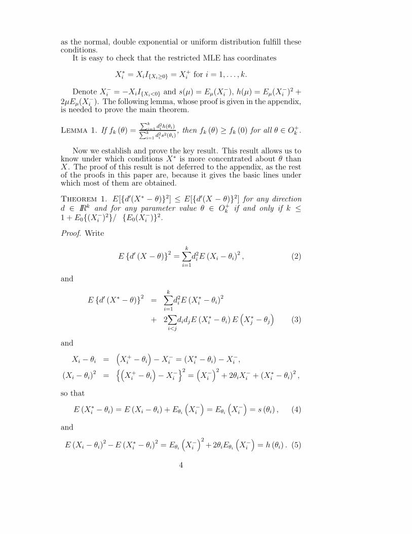
as the normal, double exponential or uniform distribution fulfill theseconditions.

It is easy to check that the restricted MLE has coordinates

X∗i = XiI{Xi≥0} = X+

i for i = 1, . . . , k.

Denote X−i = −XiI{Xi<0} and s(µ) = Eµ(X

−i ), h(µ) = Eµ(X

−i )2 +

2µEµ(X−i ). The following lemma, whose proof is given in the appendix,

is needed to prove the main theorem.

Lemma 1. If fk (θ) =∑k

i=1d2

i h(θi)∑k

i=1d2

i s2(θi), then fk (θ) ≥ fk (0) for all θ ∈ O+

k .

Now we establish and prove the key result. This result allows us toknow under which conditions X∗ is more concentrated about θ thanX. The proof of this result is not deferred to the appendix, as the restof the proofs in this paper are, because it gives the basic lines underwhich most of them are obtained.

Theorem 1. E[{d′(X∗ − θ)}2] ≤ E[{d′(X − θ)}2] for any directiond ∈ IRk and for any parameter value θ ∈ O+

k if and only if k ≤1 + E0{(X−

i )2}/ {E0(X−i )}2.

Proof. Write

E {d′ (X − θ)}2=

k∑i=1

d2i E (Xi − θi)

2 , (2)

and

E {d′ (X∗ − θ)}2=

k∑i=1

d2i E (X∗

i − θi)2

+ 2∑i<j

didjE (X∗i − θi)E

(X∗

j − θj

)(3)

and

Xi − θi =(X+

i − θi

)− X−

i = (X∗i − θi) − X−

i ,

(Xi − θi)2 =

{(X+

i − θi

)− X−

i

}2=

(X−

i

)2+ 2θiX

−i + (X∗

i − θi)2 ,

so that

E (X∗i − θi) = E (Xi − θi) + Eθi

(X−

i

)= Eθi

(X−

i

)= s (θi) , (4)

and

E (Xi − θi)2 −E (X∗

i − θi)2 = Eθi

(X−

i

)2+2θiEθi

(X−

i

)= h (θi) . (5)

4

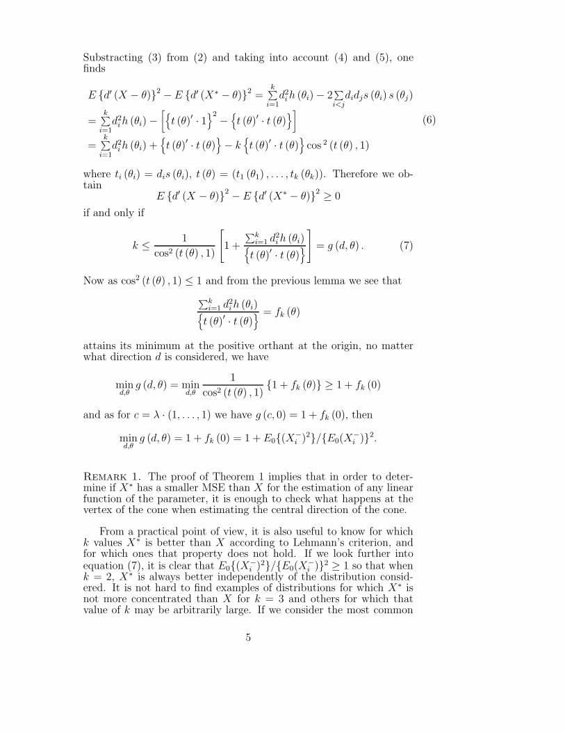
Substracting (3) from (2) and taking into account (4) and (5), onefinds

E {d′ (X − θ)}2 − E {d′ (X∗ − θ)}2 =k∑

i=1d2

i h (θi) − 2∑i<j

didjs (θi) s (θj)

=k∑

i=1d2

i h (θi) −[{

t (θ)′ · 1}2 −

{t (θ)′ · t (θ)

}]

=k∑

i=1d2

i h (θi) +{t (θ)′ · t (θ)

}− k

{t (θ)′ · t (θ)

}cos 2 (t (θ) , 1)

(6)

where ti (θi) = dis (θi), t (θ) = (t1 (θ1) , . . . , tk (θk)). Therefore we ob-tain

E {d′ (X − θ)}2 − E {d′ (X∗ − θ)}2 ≥ 0

if and only if

k ≤ 1

cos2 (t (θ) , 1)

1 +

∑ki=1 d2

i h (θi){t (θ)′ · t (θ)

} = g (d, θ) . (7)

Now as cos2 (t (θ) , 1) ≤ 1 and from the previous lemma we see that

∑ki=1 d2

i h (θi){t (θ)′ · t (θ)

} = fk (θ)

attains its minimum at the positive orthant at the origin, no matterwhat direction d is considered, we have

mind,θ

g (d, θ) = mind,θ

1

cos2 (t (θ) , 1){1 + fk (θ)} ≥ 1 + fk (0)

and as for c = λ · (1, . . . , 1) we have g (c, 0) = 1 + fk (0), then

mind,θ

g (d, θ) = 1 + fk (0) = 1 + E0{(X−i )2}/{E0(X

−i )}2.

Remark 1. The proof of Theorem 1 implies that in order to deter-mine if X∗ has a smaller MSE than X for the estimation of any linearfunction of the parameter, it is enough to check what happens at thevertex of the cone when estimating the central direction of the cone.

From a practical point of view, it is also useful to know for whichk values X∗ is better than X according to Lehmann’s criterion, andfor which ones that property does not hold. If we look further intoequation (7), it is clear that E0{(X−

i )2}/{E0(X−i )}2 ≥ 1 so that when

k = 2, X∗ is always better independently of the distribution consid-ered. It is not hard to find examples of distributions for which X∗ isnot more concentrated than X for k = 3 and others for which thatvalue of k may be arbitrarily large. If we consider the most common

5

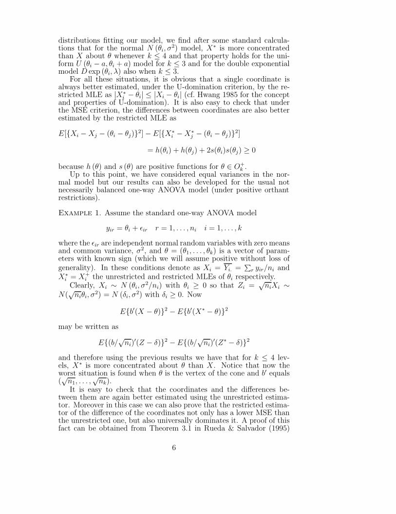
distributions fitting our model, we find after some standard calcula-tions that for the normal N (θi, σ

2) model, X∗ is more concentratedthan X about θ whenever k ≤ 4 and that property holds for the uni-form U (θi − a, θi + a) model for k ≤ 3 and for the double exponentialmodel D exp (θi, λ) also when k ≤ 3.

For all these situations, it is obvious that a single coordinate isalways better estimated, under the U-domination criterion, by the re-stricted MLE as |X∗

i − θi| ≤ |Xi − θi| (cf. Hwang 1985 for the conceptand properties of U-domination). It is also easy to check that underthe MSE criterion, the differences between coordinates are also betterestimated by the restricted MLE as

E[{Xi − Xj − (θi − θj)}2] − E[{X∗i − X∗

j − (θi − θj)}2]

= h(θi) + h(θj) + 2s(θi)s(θj) ≥ 0

because h (θ) and s (θ) are positive functions for θ ∈ O+k .

Up to this point, we have considered equal variances in the nor-mal model but our results can also be developed for the usual notnecessarily balanced one-way ANOVA model (under positive orthantrestrictions).

Example 1. Assume the standard one-way ANOVA model

yir = θi + εir r = 1, . . . , ni i = 1, . . . , k

where the εir are independent normal random variables with zero meansand common variance, σ2, and θ = (θ1, . . . , θk) is a vector of param-eters with known sign (which we will assume positive without loss ofgenerality). In these conditions denote as Xi = Yi. =

∑r yir/ni and

X∗i = X+

i the unrestricted and restricted MLEs of θi respectively.Clearly, Xi ∼ N (θi, σ

2/ni) with θi ≥ 0 so that Zi =√

niXi ∼N(

√niθi, σ

2) = N (δi, σ2) with δi ≥ 0. Now

E{b′(X − θ)}2 − E{b′(X∗ − θ)}2

may be written as

E{(b/√ni)′(Z − δ)}2 − E{(b/√ni)

′(Z∗ − δ)}2

and therefore using the previous results we have that for k ≤ 4 lev-els, X∗ is more concentrated about θ than X. Notice that now theworst situation is found when θ is the vertex of the cone and b′ equals(√

n1, . . . ,√

nk).It is easy to check that the coordinates and the differences be-

tween them are again better estimated using the unrestricted estima-tor. Moreover in this case we can also prove that the restricted estima-tor of the difference of the coordinates not only has a lower MSE thanthe unrestricted one, but also universally dominates it. A proof of thisfact can be obtained from Theorem 3.1 in Rueda & Salvador (1995)

6

taking into account that, in this situation, the direction εi − εj is inthe subspace spanned by the coordinates to be compared and that therestrictions corresponding to the rest of the coordinates do not affect,because of independence, the probabilities to be computed so that

P{|X∗i − X∗

j − (θi − θj)| ≤ t} ≥ P {|Xi − Xj − (θi − θj)| ≤ t}for all t > 0.

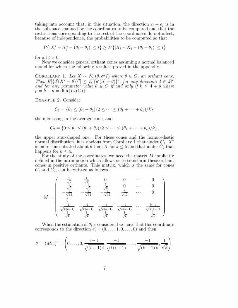
Now we consider general orthant cones assuming a normal balancedmodel for which the following result is proved in the appendix.

Corollary 1. Let X ∼ Nk (θ, σ2I) where θ ∈ C, an orthant cone.Then E[{d′(X∗ − θ)}2] ≤ E[{d′(X − θ)}2] for any direction d ∈ IRk

and for any parameter value θ ∈ C if and only if k ≤ 4 + p wherep = k − n = dim{LS(C)}.Example 2. Consider

C1 = {θ1 ≤ (θ1 + θ2)/2 ≤ · · · ≤ (θ1 + · · · + θk)/k},the increasing in the average cone, and

C2 = {0 ≤ θ1 ≤ (θ1 + θ2)/2 ≤ · · · ≤ (θ1 + · · ·+ θk)/k} ,

the upper star-shaped one. For these cones and the homocedasticnormal distribution, it is obvious from Corollary 1 that under C1, X∗is more concentrated about θ than X for k ≤ 5 and that under C2 thathappens for k ≤ 4.

For the study of the coordinates, we need the matrix M implicitlydefined in the introduction which allows us to transform these orthantcones in positive orthants. This matrix, which is the same for conesC1 and C2, can be written as follows

M =

− 1√2

1√2

0 0 · · · 0

− 1√6

− 1√6

2√6

0 · · · 0

− 1√12

− 1√12

− 1√12

3√12

· · · 0...−1√

k(k−1)

−1√k(k−1)

−1√k(k−1)

−1√k(k−1)

· · · k−1√k(k−1)

1√k

1√k

1√k

1√k

· · · 1√k

When the estimation of θi is considered we have that this coordinatecorresponds to the direction e′i = (0, . . . , 1, 0, . . . , 0) and then

b′ = (Mei)′ =

0, . . . , 0,

i − 1√(i − 1) i

,−1√

i (i + 1), . . . ,

−1√(k − 1) k

,1√k

.

7

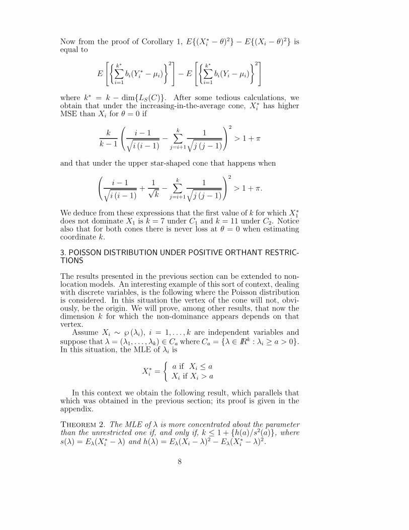
Now from the proof of Corollary 1, E{(X∗i − θ)2} − E{(Xi − θ)2} is

equal to

E

{k∗∑i=1

bi(Y∗i − µi)

}2 − E

{k∗∑i=1

bi(Yi − µi)

}2

where k∗ = k − dim{LS(C)}. After some tedious calculations, weobtain that under the increasing-in-the-average cone, X∗

i has higherMSE than Xi for θ = 0 if

k

k − 1

i − 1√

i (i − 1)−

k∑j=i+1

1√j (j − 1)

2

> 1 + π

and that under the upper star-shaped cone that happens when

i − 1√

i (i − 1)+

1√k−

k∑j=i+1

1√j (j − 1)

2

> 1 + π.

We deduce from these expressions that the first value of k for which X∗1

does not dominate X1 is k = 7 under C1 and k = 11 under C2. Noticealso that for both cones there is never loss at θ = 0 when estimatingcoordinate k.

3. POISSON DISTRIBUTION UNDER POSITIVE ORTHANT RESTRIC-TIONS

The results presented in the previous section can be extended to non-location models. An interesting example of this sort of context, dealingwith discrete variables, is the following where the Poisson distributionis considered. In this situation the vertex of the cone will not, obvi-ously, be the origin. We will prove, among other results, that now thedimension k for which the non-dominance appears depends on thatvertex.

Assume Xi ∼ ℘ (λi), i = 1, . . . , k are independent variables andsuppose that λ = (λ1, . . . , λk) ∈ Ca where Ca = {λ ∈ IRk : λi ≥ a > 0}.In this situation, the MLE of λi is

X∗i =

{a if Xi ≤ aXi if Xi > a

In this context we obtain the following result, which parallels thatwhich was obtained in the previous section; its proof is given in theappendix.

Theorem 2. The MLE of λ is more concentrated about the parameterthan the unrestricted one if, and only if, k ≤ 1 + {h(a)/s2(a)}, wheres(λ) = Eλ(X

∗i − λ) and h(λ) = Eλ(Xi − λ)2 − Eλ(X

∗i − λ)2.

8

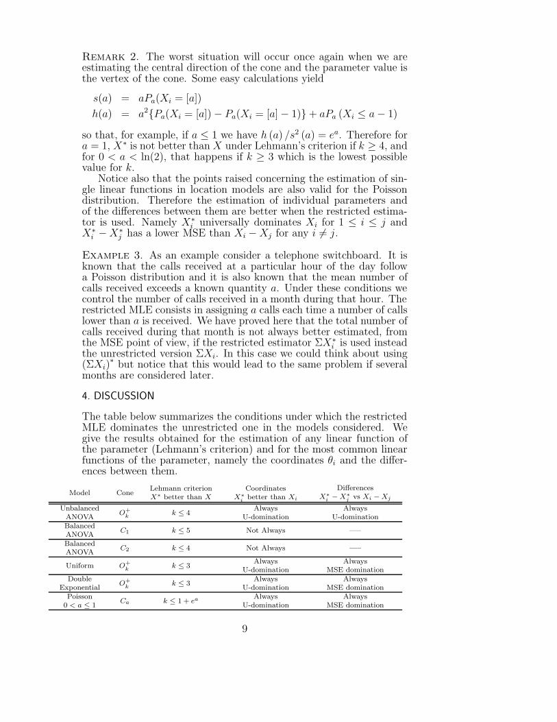
Remark 2. The worst situation will occur once again when we areestimating the central direction of the cone and the parameter value isthe vertex of the cone. Some easy calculations yield

s(a) = aPa(Xi = [a])

h(a) = a2{Pa(Xi = [a]) − Pa(Xi = [a] − 1)} + aPa (Xi ≤ a − 1)

so that, for example, if a ≤ 1 we have h (a) /s2 (a) = ea. Therefore fora = 1, X∗ is not better than X under Lehmann’s criterion if k ≥ 4, andfor 0 < a < ln(2), that happens if k ≥ 3 which is the lowest possiblevalue for k.

Notice also that the points raised concerning the estimation of sin-gle linear functions in location models are also valid for the Poissondistribution. Therefore the estimation of individual parameters andof the differences between them are better when the restricted estima-tor is used. Namely X∗

i universally dominates Xi for 1 ≤ i ≤ j andX∗

i − X∗j has a lower MSE than Xi − Xj for any i 6= j.

Example 3. As an example consider a telephone switchboard. It isknown that the calls received at a particular hour of the day followa Poisson distribution and it is also known that the mean number ofcalls received exceeds a known quantity a. Under these conditions wecontrol the number of calls received in a month during that hour. Therestricted MLE consists in assigning a calls each time a number of callslower than a is received. We have proved here that the total number ofcalls received during that month is not always better estimated, fromthe MSE point of view, if the restricted estimator ΣX∗

i is used insteadthe unrestricted version ΣXi. In this case we could think about using(ΣXi)

∗ but notice that this would lead to the same problem if severalmonths are considered later.

4. DISCUSSION

The table below summarizes the conditions under which the restrictedMLE dominates the unrestricted one in the models considered. Wegive the results obtained for the estimation of any linear function ofthe parameter (Lehmann’s criterion) and for the most common linearfunctions of the parameter, namely the coordinates θi and the differ-ences between them.

Model ConeLehmann criterionX∗ better than X

CoordinatesX∗

i better than Xi

DifferencesX∗

i − X∗j vs Xi − Xj

UnbalancedANOVA

O+k

k ≤ 4Always

U-dominationAlways

U-dominationBalancedANOVA

C1 k ≤ 5 Not Always —–

BalancedANOVA

C2 k ≤ 4 Not Always —–

Uniform O+k

k ≤ 3Always

U-dominationAlways

MSE dominationDouble

ExponentialO+

kk ≤ 3

AlwaysU-domination

AlwaysMSE domination

Poisson0 < a ≤ 1

Ca k ≤ 1 + ea AlwaysU-domination

AlwaysMSE domination

9

Table 1 makes it obvious that in none of the models considereddoes X∗ dominate X in Lehmann’s sense when k is big enough. Thishappens even though X∗ always dominates X in terms of global MSE,for instance. Given this peculiar phenomenon, some may be temptedto reject the criterion as unusual or too restrictive.

At this point, it is worth emphasizing that Lehmann’s criterionis frequently used in the linear models framework. In that context,it is usually referred to as the MSE matrix criterion or the MDE Icriterion. See, for example, Rao & Toutenburg (1995) p. 30, where theauthors explain that “As the MDE (mean dispersion error) containsall relevant information about the quality of an estimate, comparisonsbetween different estimators may be made on the basis of their MDEmatrices.” In this book, other criterions are defined from the MDEmatrix as, for example, the usual global MSE criterion, see p. 121,which is built from the trace of the MDE matrix. This criterion turnsto be obviously weaker than the previous one and is therefore referredto as the “first weak MDE criterion” in their writing.

Many times an estimator is compared to another using the weakMDE criterion, usually because it is computationally easier, and noth-ing is said about the MSE of a linear function of the parameter. Itis well known, for example, that when the estimation of a multidi-mensional normal mean is considered and k ≥ 3, the sample mean isdominated by the James-Stein estimator under the global MSE crite-rion. However it is not that often pointed out that the James-Steinestimator is not necessarily better for the estimation of all linear func-tions of the parameter.

Stein-type estimators bear some resemblance with those studied inthis paper. One similarity is that they are biased. The dominationexhibited by the restricted estimator is also somehow similar to that ofthe Stein estimator. The fact that X∗ has lower global MSE error thanX does not imply the preference of d′X∗ for the estimation of any linearfunction of the parameter d′θ. Moreover, in this paper, conditions aregiven where X∗ can be proved to be better than X using a strongcriterion such as Lehmann’s which is a result that cannot be obtainedfor Stein-type estimators. Notice also that this criterion never declaresthat X is better than X∗, nor that d′X is better than d′X∗ for theestimation of d′θ as the MSE of d′X∗ is never higher than that of d′Xfor all values of d′θ, θ ∈ O+

k .It may be argued that the conditions imposed here, independence

in particular, are not the usual ones in linear models. Nevertheless, wethink that the results obtained here are representative of what wouldhappen in the general covariance matrix case. That is, if there areproblems in the independence case it would be unlikely, we think, thatproblems would disappear in the more complex situations. The moraleof our story, therefore, is that care must be taken when a restrictedestimator is used to estimate a linear function of the parameter. Evenin the independence case, it is not hard to find examples where theestimation of θ1 + · · · + θk (central direction of the cone) may havepractical interest.

10

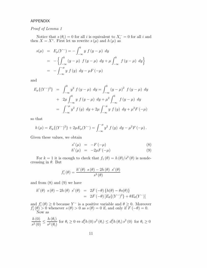
APPENDIX

Proof of Lemma 1

Notice that s (θi) = 0 for all i is equivalent to X−i = 0 for all i and

then X = X∗. First let us rewrite s (µ) and h (µ) as

s(µ) = Eµ(Y −) = −∫ 0

−∞y f (y − µ) dy

= −{∫ 0

−∞(y − µ) f (y − µ) dy + µ

∫ 0

−∞f (y − µ) dy

}

= −∫ −µ

−∞y f (y) dy − µF (−µ)

and

Eµ{(Y −)2} =∫ 0

−∞y2 f (y − µ) dy =

∫ 0

−∞(y − µ)2 f (y − µ) dy

+ 2µ∫ 0

−∞y f (y − µ) dy + µ2

∫ 0

−∞f (y − µ) dy

=∫ −µ

−∞y2 f (y) dy + 2µ

∫ −µ

−∞y f (y) dy + µ2F (−µ)

so that

h (µ) = Eµ{(Y −)2} + 2µEµ(Y−) =

∫ −µ

−∞y2 f (y) dy − µ2F (−µ) .

Given these values, we obtain

s′ (µ) = −F (−µ) (8)

h′ (µ) = −2µF (−µ) (9)

For k = 1 it is enough to check that f1 (θ) = h (θ)/s2 (θ) is nonde-creasing in θ. But

f ′1 (θ) =

h′ (θ) s (θ) − 2h (θ) s′ (θ)s3 (θ)

and from (8) and (9) we have

h′ (θ) s (θ) − 2h (θ) s′ (θ) = 2F (−θ) {h(θ) − θs(θ)}= 2F (−θ) [Eθ{(Y −)2} + θEθ(Y

−)]

and f ′1 (θ) ≥ 0 because Y − is a positive variable and θ ≥ 0. Moreover

f ′1 (θ) > 0 whenever s (θ) > 0 as s (θ) = 0 if, and only if F (−θ) = 0.

Now as

h (0)

s2 (0)≤ h (θi)

s2 (θi)for θi ≥ 0 ⇔ d2

i h (0) s2 (θi) ≤ d2i h (θi) s2 (0) for θi ≥ 0

11

we find that for θi ≥ 0, i = 1, . . . , k.

h (0)

{k∑

i=1

d2i s

2(θi)

}=

k∑i=1

d2i s

2 (θi) h (0)

≤k∑

i=1

d2i h (θi) s2(0) = s2(0)

{k∑

i=1

d2i h(θi)

}

and the lemma is proved.

Proof of Corollary 1.

From the properties of projections, the maximum likelihood esti-mator of µ is

Y ∗ = P (Y/MC) = P (MX/MC) = M · P (X/C) = MX∗,

where M is the matrix defined from (1). This estimator can also bewritten as

Y ∗i =

{Y +

i for i = 1, . . . , nYi for i = n + 1, . . . , k

(10)

Now if we denote b = Md and take into account the identityM ′M = I, we have

E[{d′(X∗ − θ)}2] − E[{d′(X − θ)}2]

= E[{(Md)′(MX∗ − Mθ)}2] − E[{(Md)′(MX − Mθ)}2]

= E[{b′(Y ∗ − µ)}2] − E[{b′(Y − µ)}2]

Moreover from (10) and the independence of the Y ∗i ,

E[{∑ki=1 bi(Y

∗i − µi)}2]

=k∑

i=1

b2i E

{(Y ∗

i − µi)2}

+k∑

i,j=1

bibjE (Y ∗i − µi) E

(Y ∗

j − µj

)

=k∑

i=1

b2i E

{(Y ∗

i − µi)2}

+n∑

i,j=1

bibjE (Y ∗i − µi) E

(Y ∗

j − µj

)

and therefore, considering once more the definition of Y ∗i given in (10),

we obtain

E[{d′(X∗ − θ)}2] − E[{d′(X − θ)}2]

= E[{n∑

i=1

bi(Y∗i − µi)}2] − E[{

n∑i=1

bi(Yi − µi)}2]

so that the result is easily obtained if we recall that for a normaldistribution fk (0) = π.

12

Proof of Theorem 2.

Following the arguments in our previous theorem, we can writeXi −a = (Xi −a)+ − (Xi −a)−, where (Xi −a)+ = max(Xi −a, 0) ≥ 0and (Xi − a)− = −min(Xi − a, 0) ≥ 0. Now

Xi − λi = (Xi − a) − (λi − a) ={(Xi − a)+ − (λi − a)

}− (Xi − a)−

= (X∗i − λi) − (Xi − a)−

and

s(λ) = Eλ(X∗i − λ) = Eλ{(Xi − a)−} = −

[a]∑k=0

(k − a) e−λ λk

k!

= aPλ(Xi ≤ a) − λPλ(X ≤ a − 1)

h(λ) = Eλ(Xi − λ)2 − Eλ(X∗i − λ)2

= Eλ{(Xi − a)−}2 + 2(λ − a)Eλ{(Xi − a)−}= λ2Pλ(Xi ≤ a − 2) + a2Pλ(Xi ≤ a) − (2a − 1)λPλ(Xi ≤ a − 1)

+ 2(λ − a) {aPλ(Xi ≤ a) − λPλ(Xi ≤ a − 1)} ,

where [a] denotes the integer part of a.From Theorem 1 and Lemma 1, it will be enough to prove that the

minimum of the function f(λ) = h(λ)/s2(λ) when λ ≥ a is reached atλ = a. As we did in that previous lemma, we will prove that f (λ) isnondecreasing in λ by checking that h′(λ)s(λ)− 2h(λ)s′(λ) ≥ 0. Sometedious calculations yield

s(λ) = aPλ(X = [a]) − (λ − a)Pλ(X ≤ [a] − 1)

s′(λ) = ([a] − a)Pλ(X = [a]) − Pλ(X ≤ [a] − 1)

h(λ) = {a(λ − a) + λ(a − [a])}Pλ(X = [a])

+ {λ − (λ − a)2}Pλ(X ≤ [a] − 1)

h′(λ) = {a(a − 2λ + 2) − [a]([a] − 2λ + 2)}Pλ(X = [a])

+ (2a − 2λ + 1)Pλ(X ≤ [a] − 1)

and then after some more calculations, h′(λ)s(λ) − 2h(λ)s′(λ) is seento equal

Pλ(X ≤ [a]−1)Pλ(X = [a]) {a + 2(λ + a)(a − [a]) + (λ − a)(a − [a])2}

+ P 2λ (X = [a])

{(a − [a])2(2λ − a) + 2a(a − [a])

}+ P 2

λ (X ≤ [a] − 1)(λ + a)

where the three factors are positive and the theorem is done.

13

ACKNOWLEDGEMENTS

This research was partially supported by Spanish DGES grant PB97-0475 and by PAPIJCL grant VA26/99. The authors are grateful tothe Editor, the Associate Editor and two referees for their suggestionsand comments which led to this improved version of the paper.

REFERENCES

Abelson, R. P., & Tukey, J. W. (1963). Efficient utilization of non-numerical information in quantitative analysis: General theory andthe case of the simple order. Ann. Math. Statist., 34, 1347–1369.

Dykstra, R. L., & Robertson, T. (1983). On testing monotone tendencies.J. Amer. Statist. Assoc., 78, 342–350.

Fernandez, M. A., Rueda, C., & Salvador B. (1999). The loss of efficiencyestimating linear functions under restrictions. Scand. J. Statist., inpress.

Geweke, J. (1986). Exact inference in the inequality constrained normallinear regression model. J. Applied Econometrics, 1, 127–141.

Hwang, J. T. (1985). Universal domination and stochastic domination:Estimation simultaneously under a broad class of loss functions. Ann.Statist., 13, 295–314.

Hwang, J. T., & Peddada, S. D. (1994). Confidence interval estimationsubject to order restrictions. Ann. Statist., 22, 67–93.

Lehmann, E. L. (1983). Theory of Point Estimation. John Wiley, NewYork.

Rao, C. R., & Toutenburg, H. (1995). Linear Models. Least Squares andAlternatives. Springer-Verlag, New York.

Robertson, T., Wright, F. T., & Dykstra, R. L. (1988). Order RestrictedStatistical Inference. John Wiley, New York.

Rueda, C., & Salvador, B. (1995). Reduction of risk using restricted esti-mators. Comm. Statist. Theory and Meth., 24, 1011–1023.

Shaked, M. (1979). Estimation of starshaped sequences of Poisson andnormal means. Ann. Statist., 7, 729–741.

Received 18 November 1998 Departamento de Estadıstica e I.O.Accepted 29 June 1999 Universidad de Valladolid

47005 ValladolidEspana

e-mail: [email protected]

14