Parameter estimation of delay differential equations: an integration-free LS-SVM approach

Parameter estimation of delay differential equations:an integration-free LS-SVM approach

Siamak Mehrkanoona,∗, Saeid Mehrkanoonb, Johan A.K. Suykensa

aKU Leuven, ESAT-SCD, Kasteelpark Arenberg 10, B-3001 Leuven (Heverlee), Belgium,Email: siamak.mehrkanoon,[email protected]

bUniversity of New South Wales, Black Dog Institute, Hospital Rd, Randwick, NSW 2031, Australia, Email:[email protected]

Abstract

This paper introduces an estimation method based on Least Squares Support Vector Machines (LS-SVMs) for ap-proximating time-varying as well as constant parameters indeterministic parameter-affine delay differential equations(DDEs). The proposed method reduces the parameter estimation problem to an algebraic optimization problem. Thus,as opposed to conventional approaches, it avoids iterativesimulation of the given dynamical system and therefore asignificant speedup can be achieved in the parameter estimation procedure. The solution obtained by the proposedapproach can be further utilized for initialization of the conventional nonconvex optimization methods for parameterestimation of DDEs. Approximate LS-SVM based models for thestate and its derivative are first estimated from theobserved data. These estimates are then used for estimationof the unknown parameters of the model. Numericalresults are presented and discussed for demonstrating the applicability of the proposed method.

Keywords: Delay differential equations, Parameter identification, Least squares support vector machines,Closed-form approximation

1. Introduction

Delay differential equations (DDEs) have been successfully used in the mathematical formulation of real lifephenomena in a wide variety of applications especially in science and engineering such as population dynamics,infectious disease, control problems, secure communication, traffic control and economics [1, 2, 3]. In contrast withordinary differential equations (ODEs) where the unknown function and its derivatives are evaluated at the same timeinstant, in a DDE the evolution of the system at a certain timeinstant, depends on the state of the system at an earliertime. A typical first order single-delay scalar DDE model maybe expressed as:

x(t) = f1(t, x(t), x(t − τ1), θ(t)), t ≥ tin,

x(t) = H1(t), ρ ≤ t ≤ tin(1)

whereH1(t) is the initial function (history function),τ1 is the delay or lag which is non-negative and can in generalbe constant, time dependent or state dependent i.e.τ1 = τ1(t, x(t)) andρ = min

t≥tint− τ1. The termx(t− τ1) is called the

delay term. In more general models, the derivative ˙x(t) may depend onx(t) andx(t) itself at some past valuet − τ1. Inthis case equation (1) can be rewritten in a more general formas follows

x(t) = f2(t, x(t), x(t − τ1), x(t − τ2), θ(t)), t ≥ tin,

x(t) = H2(t), ρ ≤ t ≤ tin(2)

∗Corresponding authorEmail address:[email protected] (Siamak Mehrkanoon )

Preprint submitted to Commun Nonlinear Sci Numer Simulat October 23, 2013

whereρ = min1≤i≤2min

t≥tin(t−τi). Equation (2) is called delay differential equation of neutral type (NDDE). Models (1) and

(2) usually involve some unknown parameters that require tobe estimated from the observational data. We considersetsθ(t),H1(t), τ1 andθ(t),H2(t), τ1, τ2 as parameters of the models (1) and (2) respectively.

Identification of unknown parameters in differential equations has been studied and addressed by many authors(see [4, 5, 6, 7, 8, 9]). Most of the available approaches utilize the classical parametric inference such as the leastsquares estimator or the maximum likelihood estimation [10]. In these approaches first the dynamical system issimulated using initial guesses for the parameters. Then model predictions are compared with measured data and anoptimization algorithm updates the parameters. Thereforeconsidering the dynamical system (1) one has to solve thefollowing optimization problem:

argminθ(t),τ1

J(θ(t), τ1) =N∑

k=1

(ym(tk) − yp(tk))2, (3)

whereym(t) andyp(t) are the measured data and model prediction respectively. It should be noted that the objectivefunction of the optimization problem for DDE differs from that of ODE. The cost functionJ(θ(t), τ1) in (3) might benon-smooth because the state trajectory might be non-smooth in the parameter and this will make the optimizationproblem more complicated.

Solving (3) requires repeated simulation of the system of DDE under study. Since the analytic solution of DDEis usually not available, therefore one needs to apply a numerical algorithm to simulate the given dynamic system.Although quite efficient numerical routines for solving differential equations are available they usually slow downthe parameterization process dramatically and this situation is even more sensible when the underlying dynamic isdescribed by delay differential equations. That is due to the existence of delay terms that force the solver to usean interpolation technique in order to advance the solution. It should also be noted that, as opposed to ordinarydifferential equation, the numerical solution of DDE not only depends on the parameter values, but also on the historyfunction,H1(t) for t ∈ [ρ, tin], which is usually unknown. Given that the initial functionis an infinite-dimensional set,the problem becomes an infinite-dimensional optimization problem and very difficult to solve [11]. Consequently, itwould be of great benefit to eliminate any need of numerical DDE solvers.

Varah [13], proposed an approach for time-invariant parameter estimation of ODEs that does not require repeatednumerical integration and is referred to as a two-step approach. First a cubic spline is used to estimate the systemdynamics and its derivative from observational data. In thesecond step these estimates are plugged into a givendifferential equation and the unknown parameters are found by minimizing the squared difference of both sides of thedifferential equation.

The authors in [12] first estimate the derivative ˙x(t) from the noisy data using nonparametric smoothing methodsand then inferred the constant delayτ, for a special DDE model, in the framework of the generalizedadditive model.

The author in [14] proposed a method where an artificial neural network model is used to estimate the timeinvariant parameters of a dynamical systems governed by ordinary differential equations. Despite the fact that theclassical neural networks have nice properties such as universal approximation, they still suffer from having twopersistent drawbacks. The first problem is the existence of many local minima solutions. The second problem is howto choose the number of hidden units.

The parameter estimation in ordinary differential equations using least squares support vector machines is stud-ied in [15]. It is the aim of this paper to extend the method proposed in [15] for estimating the unknown timevarying/invariant parameters in parameter-affine delay differential equations for both non-neutral and neutral cases.Throughout this paper, we assume that the dynamical system is uniquely solvable and that the parameters of the modelare identifiable. For stability of the solutions of systems with delays one may refer to [16, 17].

The paper is organized as follows. In section 2, the problem statement is given. In section 3, estimation of thestate trajectory and its derivative by means of least squares support vector machines is discussed. Section 4 describesleast squares support vector machines formulation to approximate the time varying/invariant parameters in DDEs andNDDEs. In section 5, examples are given in order to confirm thevalidity and applicability of the proposed method.

2

2. Problem statement

2.1. Reconstruction of fixed delays

Consider the dynamics of a process during a given time interval modeled by a system of nonlinear DDEs withassociated history functionsH(t) of the form:

x(t) = f (t, x(t), x(t − τ1), x(t − τ2), . . . , x(t − τp)), t ≥ tin,

x(t) = H(t), ρ ≤ t ≤ tin(4)

whereρ = min1≤i≤pmin

t≥tin(t − τi), x(t) ∈ R

n and the delaysτipi=1 are constant and unknown. In order to estimate the

model parameters, all the states of the system are measured i.e. y(ti) = x(ti) + e(ti) wheree(ti)Ni=1 are independentmeasurement errors with zero mean. Throughout this paper a particular structure of (4) is considered. It is assumedthat nonlinear model (4) exhibits the parameter-affine form i.e. it is affine in thex(t − τi) for i = 1, . . . , p.

2.2. Reconstruction of time varying parameters

Consider the nonlinear state-dependent delay differential equation given in (1) with associated history functionH1(t). In order to estimate the unknown parameters, a set of measurementsy(ti) are collected. In general the set ofmeasurementsy(ti) do not necessarily correspond to the model statesx(ti). However here it is assumed that the systemstates are measured with measurement errore(ti), therefore the sate space model has the following form:

x(t) = f1(t, x(t), x(t − τ1), θ(t)), t ≥ tin,

y(ti) = x(ti) + ei , i = 1, . . . ,N(5)

wherey(t) is the output of the system which has been observed atN time instants andeiNi=1 are independent mea-

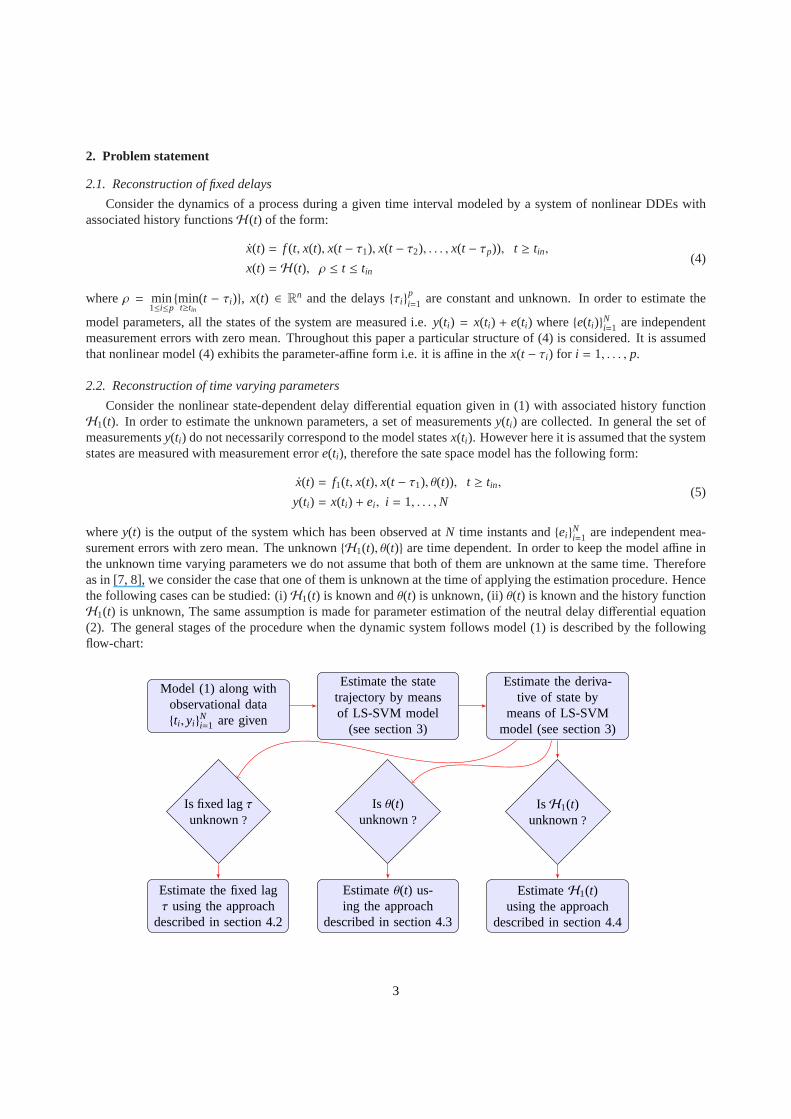
surement errors with zero mean. The unknownH1(t), θ(t) are time dependent. In order to keep the model affine inthe unknown time varying parameters we do not assume that both of them are unknown at the same time. Thereforeas in [7, 8], we consider the case that one of them is unknown atthe time of applying the estimation procedure. Hencethe following cases can be studied: (i)H1(t) is known andθ(t) is unknown, (ii)θ(t) is known and the history functionH1(t) is unknown, The same assumption is made for parameter estimation of the neutral delay differential equation(2). The general stages of the procedure when the dynamic system follows model (1) is described by the followingflow-chart:

Model (1) along withobservational datati , yi

Ni=1 are given

Estimate the statetrajectory by meansof LS-SVM model

(see section 3)

Estimate the deriva-tive of state by

means of LS-SVMmodel (see section 3)

IsH1(t)unknown?

Is θ(t)unknown?

Is fixed lagτunknown?

EstimateH1(t)using the approach

described in section 4.4

Estimateθ(t) us-ing the approach

described in section 4.3

Estimate the fixed lagτ using the approach

described in section 4.2

3

3. Estimation of the state trajectory and its derivative

Let us consider a given training setti , yiNi=1 with input datati ∈ R and output datayi ∈ R that are obtained from

(5). The goal in regression is to estimate a model of the form ˆx(t) = wTϕ(t) + b. The primal LS-SVM model forregression can be written as follows [18, 19]

minimizew,b,e

12

wTw+γ

2eTe

subject to yi = wTϕ(ti) + b+ ei , i = 1, ...,N(6)

whereγ ∈ R+,b ∈ R, w ∈ Rh. ϕ(·) : R→ Rh is the feature map andh is the dimension of the feature space. The dual

solution is then given by

Ω + IN/γ 1N

1TN 0

α

b

=

y

0

whereΩi j = K(ti , t j) = ϕ(ti)Tϕ(t j) is the (i, j)-th entry of the positive definite kernel matrix. 1N = [1, . . . ,1]T ∈ RN,

α = [α1, . . . , αN]T , y = [y1, . . . , yN]T andIN is the identity matrix. The model in dual form becomes:

x(t) = wTϕ(t) + b =N∑

i=1

αiK(ti , t) + b, (7)

whereK is the kernel function. Making use of Mercer’s theorem [20],derivatives of the feature map can be writtenin terms of derivatives of the kernel function. Therefore one can obtain a closed-form approximate expression for thederivative of the model (7) with respect to time as follows [21],

ddt

x(t) =wT ϕ(t) =N∑

i=1

αiKs(ti , t), (8)

whereKs(t, s) =∂(ϕ(t)Tϕ(s))

∂s .

4. Parameter estimation of DDE

4.1. General Methodology

The proposed scheme will make use of the LS-SVM ability to provide a closed-form approximation for the statetrajectory and its derivative from measured data. We approximate the trajectory ˆx(t) on the basis of observations atNpointsti , y(ti)Ni=1 using (7). Then (8) is utilized for approximating the state derivative. These closed-form expressionswill be used later in the process of parameter estimation.

4.2. Fixed delayτ is unknown

For the sake of simplicity the methodology is described for ascalar DDE with single delay, but the approach isapplicable for identifying multi-delays in a system of DDEsprovided that they are identifiable. Consider the followingsingle delay parameter-affine DDE:

x(t) = f (t, x(t))x(t − τ), t ≥ tin, (9)

where f (·) : R2 −→ R is an arbitrary nonlinear function andτ is the constant parameter of the system which is

unknown. In order to estimate the unknownτ value, the state of the system is measured i.e.y(ti) = x(ti) + e(ti) wheree(ti)Ni=1 are independent measurement errors with zero mean. Let us assume an explicit LS-SVM model

xτ(t) = vTψ(t) + d,

4

as an approximation for the termx(t − τ) whereψ(·) : R → Rh is the feature map. Substituting the closed-form

expressions for the state and its derivative,ddt x(t) and x(t) obtained from (7) and (8) respectively, into the model

description (9), the sought parametersv andd are identified as those minimizing the following optimization problem:

minimizev,d,e

12

vTv+γ

2

M∑

i=1

e2i

subject toddt

x(ti) =(

vTψ(ti) + d)

f (ti , x(ti)) + ei , for i = 1, ...,M.

(10)

Remark 4.1. Since closed-form expressions for the state and its derivative are available we are not limited to chooseM = N, i.e. we can evaluate the constraint of the above optimization problem at the time instant ti which is notnecessarily the same as time instants that the system is measured.

Lemma 4.1. Given a positive definite kernel functionK : R × R → R with K(t, s) = ψ(t)Tψ(s) and a regularizationconstantγ ∈ R+, the solution to (10) is given by the following dual problem

DΩD + γ−1I F

FT 0

α

d

=

dxdt

0

(11)

whereΩ(i, j) = K(ti , t j) = ψ(ti)Tψ(t j) is the(i, j)-th entry of the positive definite kernel matrix and I is the identitymatrix. Alsoα = [α1, . . . , αM]T , F = [ f (t1, x(t1)), . . . , f (tM , x(tM))]T , dx

dt = [ ddt x(t1), . . . , d

dt x(tM)]T . D is a diagonalmatrix with the elements of F on the main diagonal.

Proof 4.1. The Lagrangian of the constrained optimization problem (10) becomes

L(v,d,ei , αi) =12

vTv+γ

2

M∑

i=1

e2i −

M∑

i=1

αi

[(

vTψ(ti) + d)

f (ti , x(ti)) + ei −ddt

x(ti)]

,

where

αiMi=1 are Lagrange multipliers. Then the Karush-Kuhn-Tucker (KKT) optimality conditions are as follows,

∂L

∂v= 0→ v =

M∑

i=1

αi f (ti , x(ti))ψ(ti),

∂L

∂d= 0→

M∑

i=1

αi f (ti , x(ti)) = 0,

∂L

∂ei= 0→ ei =

αi

γ, i = 1, . . . ,M,

∂L

∂αi= 0→

(

vTψ(ti) + d)

f (ti , x(ti)) + ei =ddt

x(ti), for i = 1, . . . ,M.

After elimination of the primal variables v andeiMi=1 and making use of Mercer’s Theorem, the solution is given in

the dual by

ddt x(ti) =

M∑

j=1

α j f (t j , x(t j))Ω ji f (ti , x(ti)) +αi

γ+ d f(ti , x(ti)), i = 1, . . . ,M

0 =M∑

i=1

αi f (ti , x(ti))

Writing these equations in matrix form gives the linear system in (11).

The model in the dual form becomes

xτ(t) = vTψ(t) + d =M∑

i=1

αi f (ti , x(ti))K(ti , t) + d, (12)

whereK is the kernel function.

5

Remark 4.2. If one is not interested in having a closed-form approximation to the term x(t− τ), an alternative way toobtain an approximation for x(t − τ) at the time instant ti is by using (9) directly, i.e. x(ti − τ) = d

dt x(ti)−1 f (ti , x(ti)). Asimilar strategy can be applied in the case that the dynamicsof the process is described by a system of delay differentialequations. After substituting the closed-form expressions for the states and their derivatives into the model, then onehas to solve a system of linear equations (provided that the underlying system is affine in the unknown parameter) toobtain the approximation of the delay terms x(t − τ j) for j = 1, . . . , p at time instants t= ti , for i = 1, . . . ,N.

After obtaining the estimation ˆxτ(t), the task is to estimate the fixed delayτ. To this end, let us first define a shiftingoperator∆m(·) which will be used in the process of estimation of the delayτ. Operator∆m(·) shifts the given timeseries, which in our problem setting can for example be ˆx(t) or ˆx(t), msteps forward in time in a certain manner, whilekeeping the length of the time series unchanged. This is doneby adding a constant vector of sizem (whose values willbe clarified later) from the left to the time series and removing them last elements of the time series simultaneously.Therefore, given the time series ˆx(t) = [ x(t1), x(t2), . . . , x(tN)]T , operator∆m(·) is defined as follows:

z(t) = ∆m(x(t)) =

[z(t1), z(t2), . . . , z(tm)︸ ︷︷ ︸

Constant vector

, x(t1), x(t2), . . . , x(tN−m)]T , for 1 ≤ m≤ N − 1

x(t), for m= 0(13)

with z(t1) = z(t2) = . . . , z(tm) = c wherec is a constant. Noting that in an ideal case (noise free) one can expect a delaydifferential equation to have the following property

xτ(t)

t=τ

= x(t)

t=tin

, for τ ≥ 0, (14)

it is natural to utilize the first element of ˆx(t), i.e., x(t1) as a constantc used in operator∆m(·). In order to estimate thedelayτ, we use the sample correlation coefficient function defined as:

rzxτ =

∑Ni=1(z(ti) − µ1)(xτ(ti) − µ2)

√∑N

i=1(z(ti) − µ1)2√∑N

i=1(xτ(ti) − µ2)2, (15)

whereµ1 andµ2 denote the sample mean of time seriesz(t) and xτ(t) respectively. Given ˆx(t) and xτ(t) the process ofestimating the unknown delayτ is described in Algorithm 1.

Algorithm 1: Approximating the constant delay of a given DDEInput: Time series ˆx(t) and xτ(t) of sizeN; sampling timeTs (in seconds).Output: Time delayτ

1 for m← 0 to N − 1 do2 z(t)← ∆m(x(t))3 R(m)← Corrcoef(z(t), xτ(t))

4 τ← Ts × argmaxm

R(m)

5 return τ

In Algorithm 1, Corrcoef is a Matlab built-in function that computes the correlationcoefficient of two signalsandR(m) corresponds torzxτ . One may notice that in this approach we are not using the history function for estimatingthe time delayτ. But if the history function is known a priori, one may use it for constructing the constant vector usedin operator∆m(·) by taking the value of history function at timetin.

4.3. Parameterθ(t) is unknown

Consider model (1) and case (i) where the time varying parameter θ(t) is unknown and delayτ1 is known. There-fore with a slight abuse of notation, let us assume an explicit LS-SVM model

θ(t) = vTψ(t) + d,

6

as an approximation for the parameterθ(t). The adjustable parametersv andd are to be found by solving the followingoptimization problem

minimizev,d,e,ǫ,θi

12

vTv+γ

2(

M∑

i=1

e2i +

M∑

i=1

ǫ2i )

subject toddt

x(ti) = f1(ti , x(ti), x(ti − τ1), θi) + ei , for i = 1, . . . ,M,

θi = vTψ(ti) + d + ǫi , for i = 1, . . . ,M.

(16)

Here the obtained closed-form expressions for the state andits derivative,ddt x(t) andx(t) obtained from (7) and (8), are

substituted into the model description (1). Iff1 is nonlinear inθ(t) then the above optimization problem is non-convex.The solution of (16) in the dual can be obtained by solving a system of nonlinear equations. However, throughout thispaper, we present our results for the case that the nonlinearmodel (1) is affine in the parameterθ(t). More preciselywe consider the following parameter-affine form of (1)

x(t) = θ(t) f1(t, x(t), x(t − τ1)), t ≥ tin,

x(t) = H1(t), t ≤ tin.

This will result in the following convex optimization problem:

minimizev,d,e

12

vTv+γ

2

M∑

i=1

e2i

subject toddt

x(ti) =(

vTψ(ti) + d)

f1(ti , x(ti), x(ti − τ1)) + ei , for i = 1, . . . ,M.

(17)

Lemma 4.2. Given a positive definite kernel functionK : R × R → R with K(t, s) = ψ(t)Tψ(s) and a regularizationconstantγ ∈ R+, the solution to (17) is given by the following dual problem

DΩD + γ−1I F1

FT1 0

α

d

=

dxdt

0

(18)

whereΩ(i, j) = K(ti , t j) = ψ(ti)Tψ(t j) is the(i, j)-th entry of the positive definite kernel matrix and I is the identity ma-trix. Alsoα = [α1, . . . , αM]T , F1 = [ f1(t1, x(t1), x(t1−τ1)), . . . , f1(tM , x(tM), x(tM −τ1))]T , dx

dt = [ ddt x(t1), . . . , d

dt x(tM)]T .D is a diagonal matrix with the elements of F1 on the main diagonal.

The model in the dual form becomes:

θ(t) =M∑

i=1

αi f1(ti , x(ti), x(ti − τ1))K(ti , t) + d, (19)

whereK is the kernel function.

Proof 4.2. The approach is the same as in proof of Lemma 4.1.

It should be noted that in the process of estimatingθ(t), the values of the history functionH1(t) are not used.ThereforeH1(t) can also be unknown whileθ(t) is being estimated which is the advantage of the proposed methodcompared with conventional approaches that require the history function for simulating the underlying model.

Remark 4.3. The same procedure can be applied for estimating the unknownparameterθ(t) in parameter-affine formof model (2).

7

4.4. History functionH1(t) is unknown

Consider model (1) and case (ii) where the parameterH1(t) is unknown and all the other parameters are known. Itis assumed that the nonlinear functionf1 is affine inx(t − τ1). More precisely we consider the following form of (1):

x(t) = x(t − τ1) f1(t, x(t), θ(t)), t ≥ tin,

x(t) = H1(t), t ≤ tin(20)

whereτ1 can be time and state dependent. Since the history function is time varying let us, with a slight abuse ofnotation, assume an explicit LS-SVM model

H1(t) = vTψ(t) + d,

as an approximation to the trueH1(t). Optimal value forv andd can be obtained by solving the following convexoptimization problem:

minimizev,d,e

12

vTv+γ

2

|T|∑

i=1

e2i

subject toddt

x(tisel) =(

vTψ(tisel) + d)

f1(tisel, x(tisel), θ(tisel)) + ei , for i = 1, . . . , |T|,

(21)

where ddt x(tisel) and x(tisel) are estimations of the state trajectory and its derivativeobtained by using LS-SVM models

(7) and (8) respectively.|T| is the cardinality of the ordered setT = t1sel, t2sel, . . . , t

|T|

sel whose elements are selectedusing Algorithm 2.

Algorithm 2: Approximating the model’s time varying history function

Input: VectorT consists of time instantstiNi=1 and the delayτ1

Output: setT1 for i ← 1 to N do2 tlag(i)← ti − τ1(ti)

3 Find a vector of indices of elements oftlag whose values are less thantin (assuming thattin = t1)4 T ← elements ofT corresponding to the indices found in step 2.5 return T

The solution to (21) in the dual can be obtained by solving linear system (18) withα = [α1, . . . , α|T|]T , F1 =

[ f1(t1sel, x(t1sel), θ(t1sel)), . . . , f1(t|T|sel, x(t|T|sel), θ(t

|T|

sel))]T and dx

dt = [ ddt x(t1sel), . . . ,

ddt x(t|T|sel)]

T . D is a diagonal matrix with theelements ofF1 on the main diagonal. The model in the dual form becomes:

H1(t) =|T|∑

i=1

αi f1(tisel, x(tisel), θ(tisel))K(ti , t) + d, (22)

whereK is the kernel function. If delayτ1 in the model (20) is constant, one can first utilize Algorithm1 to estimatethe delayτ1 and then apply Algorithm 2 to obtain a closed-form approximation to the history functionH1(t).

Remark 4.4. The same procedure can be applied for estimating the unknownhistory functionH2(t) in a parameter-affine form of model (2).

5. Experiments

In this section, six experiments are performed to demonstrate the capability of the proposed method for timevarying/invariant parameters of parameter-affine non-neutral DDEs and neutral DDEs. The last three test problemsare taken from [7] and [8], but in contrast with the approach given in these references, we allow to have measurement

8

errors. The performance of the LS-SVM model depends on the choice of the tuning parameters. In this paper, for

all experiments, the Gaussian RBF kernel i.e.K(x, y) = exp(−‖x−y‖22σ2 ) is used. Therefore, a model is determined by

the regularization parameterγ and the kernel bandwidthσ. The 10-fold cross validation criterion is used to tunethese parameters. The SNR stands for signal to noise ratio which is calculated using 20 log10(

Asignal

Anoise) whereAsignal and

Anoise are the root mean square of the signal and noise respectively. The estimated parameter values are obtained byaveraging over 10 simulation runs. As error bounds we used about twice the standard deviation of the error.

5.1. Constant parameters

Problem 5.1. Consider a Kermack-McKendrick model of an infectious disease with periodic outbreak [22, Ex-ample 1]

x1(t) = −x1(t)x2(t − τ1) + x2(t − τ2)

x2(t) = x1(t)x2(t − τ1) − x2(t)

x3(t) = x2(t) − x2(t − τ2)

(23)

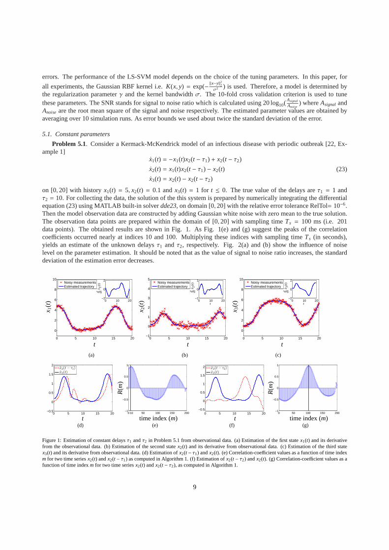
on [0,20] with history x1(t) = 5, x2(t) = 0.1 andx3(t) = 1 for t ≤ 0. The true value of the delays areτ1 = 1 andτ2 = 10. For collecting the data, the solution of the this system is prepared by numerically integrating the differentialequation (23) using MATLAB built-in solverdde23, on domain [0,20] with the relative error tolerance RelTol= 10−6.Then the model observation data are constructed by adding Gaussian white noise with zero mean to the true solution.The observation data points are prepared within the domain of [0,20] with sampling timeTs = 100 ms (i.e. 201data points). The obtained results are shown in Fig. 1. As Fig. 1(e) and (g) suggest the peaks of the correlationcoefficients occurred nearly at indices 10 and 100. Multiplying these indices with sampling timeTs (in seconds),yields an estimate of the unknown delaysτ1 and τ2, respectively. Fig. 2(a) and (b) show the influence of noiselevel on the parameter estimation. It should be noted that asthe value of signal to noise ratio increases, the standarddeviation of the estimation error decreases.

0 5 10 15 20

0

2

4

6

8

10

0 10 20−2

0

2Noisy measurementsEstimated trajectory

t

x 1(t

)

d dtx 1

(t)

t

(a)

0 5 10 15 20−1

0

1

2

3

4

5

0 10 20−1

0

1Noisy measurementsEstimated trajectory

t

d dtx 2

(t)

x 2(t

)

t

(b)

0 5 10 15 20

0

2

4

6

8

10

0 10 20−2

0

2Noisy measurementsEstimated trajectory

t

d dtx 3

(t)

x 3(t

)

t

(c)

0 5 10 15 20−0.5

0

0.5

1

1.5

2

x2(t− τ1)x2(t)

t(d)

0 10 50 100 150 200−1

−0.5

0

0.5

1

R(m

)

time index (m)(e)

0 5 10 15 20−0.5

0

0.5

1

1.5

2

x2(t− τ2)x2(t)

t(f)

0 50 100 150 200−1

−0.5

0

0.5

1

R(m

)

time index (m)(g)

Figure 1: Estimation of constant delaysτ1 andτ2 in Problem 5.1 from observational data. (a) Estimation of thefirst statex1(t) and its derivativefrom the observational data. (b) Estimation of the second state x2(t) and its derivative from observational data. (c) Estimationof the third statex3(t) and its derivative from observational data. (d) Estimationof x2(t − τ1) andx2(t). (e) Correlation-coefficient values as a function of time indexm for two time seriesx2(t) andx2(t − τ1) as computed in Algorithm 1. (f) Estimation ofx2(t − τ2) andx2(t). (g) Correlation-coefficient values as afunction of time indexm for two time seriesx2(t) andx2(t − τ2), as computed in Algorithm 1.

9

30 24 18 15

0

1

2

3

4

5

τ1

SNR

(a)

30 24 18 159.9

9.95

10

10.05

10.1

10.15

10.2

τ2

SNR

(b)

31 20 16 13

1

1.2

1.4

1.6

1.8

2

τ

SNR

(c)

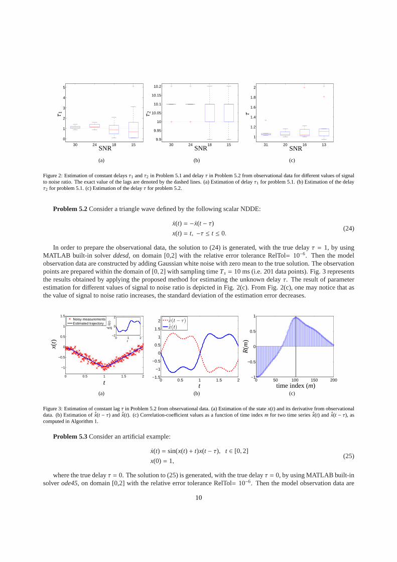
Figure 2: Estimation of constant delaysτ1 andτ2 in Problem 5.1 and delayτ in Problem 5.2 from observational data for different values of signalto noise ratio. The exact value of the lags are denoted by the dashed lines. (a) Estimation of delayτ1 for problem 5.1. (b) Estimation of the delayτ2 for problem 5.1. (c) Estimation of the delayτ for problem 5.2.

Problem 5.2 Consider a triangle wave defined by the following scalar NDDE:

x(t) = −x(t − τ)

x(t) = t, −τ ≤ t ≤ 0.(24)

In order to prepare the observational data, the solution to (24) is generated, with the true delayτ = 1, by usingMATLAB built-in solver ddesd, on domain [0,2] with the relative error tolerance RelTol= 10−6. Then the modelobservation data are constructed by adding Gaussian white noise with zero mean to the true solution. The observationpoints are prepared within the domain of [0,2] with sampling timeTs = 10 ms (i.e. 201 data points). Fig. 3 representsthe results obtained by applying the proposed method for estimating the unknown delayτ. The result of parameterestimation for different values of signal to noise ratio is depicted in Fig. 2(c). From Fig. 2(c), one may notice that asthe value of signal to noise ratio increases, the standard deviation of the estimation error decreases.

0 0.5 1 1.5 2

−1

−0.5

0

0.5

1

1.5

0 1 2−2

0

2Noisy measurementsEstimated trajectory

t

x(t)

d dtx(

t)

t

(a)

0 0.5 1 1.5 2−1.5

−1

−0.5

0

0.5

1

1.5

2

ˆx(t− τ)ˆx(t)

t(b)

0 50 100 150 200−1

−0.5

0

0.5

1

R(m

)

time index (m)(c)

Figure 3: Estimation of constant lagτ in Problem 5.2 from observational data. (a) Estimation of thestatex(t) and its derivative from observationaldata. (b) Estimation ofx(t − τ) and ˆx(t). (c) Correlation-coefficient values as a function of time indexm for two time seriesx(t) and ˆx(t − τ), ascomputed in Algorithm 1.

Problem 5.3 Consider an artificial example:

x(t) = sin(x(t) + t)x(t − τ), t ∈ [0,2]

x(0) = 1,(25)

where the true delayτ = 0. The solution to (25) is generated, with the true delayτ = 0, by using MATLAB built-insolverode45, on domain [0,2] with the relative error tolerance RelTol= 10−6. Then the model observation data are

10

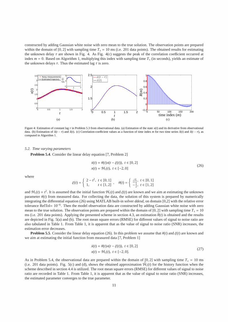
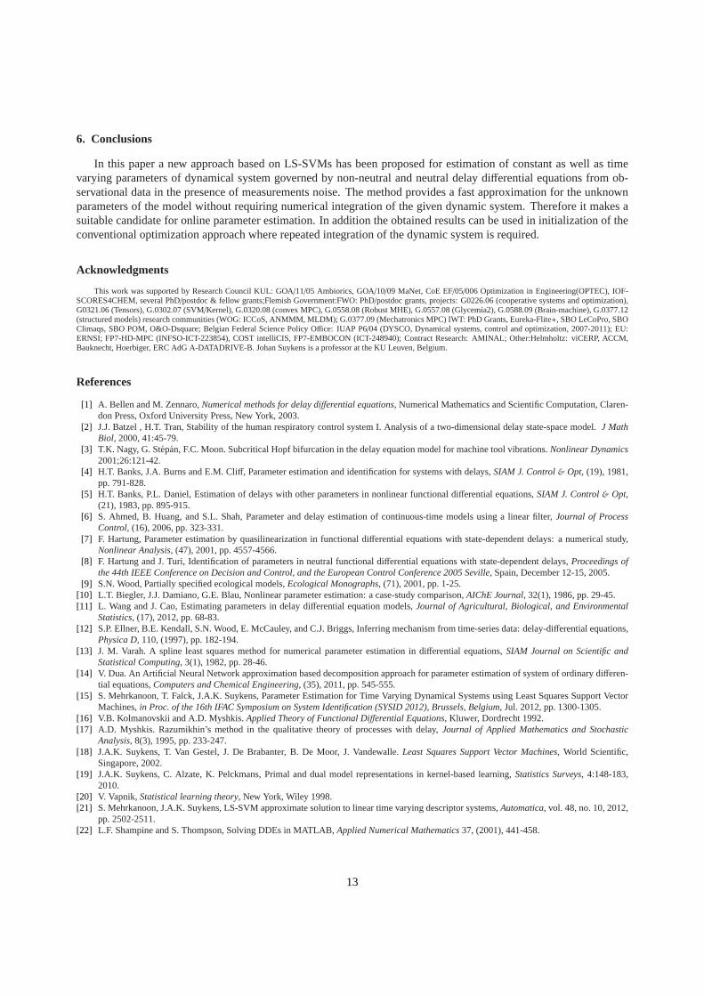
constructed by adding Gaussian white noise with zero mean tothe true solution. The observation points are preparedwithin the domain of [0,2] with sampling timeTs = 10 ms (i.e. 201 data points). The obtained results for estimatingthe unknown delayτ are shown in Fig. 4. As Fig. 4(c) suggests the peak of the correlation coefficient occurred atindexm= 0. Based on Algorithm 1, multiplying this index with sampling timeTs (in seconds), yields an estimate ofthe unknown delaysτ. Thus the estimated lagτ is zero.

0 0.5 1 1.5 20

0.5

1

1.5

2

2.5

3

3.5

0 1 2−2

0

2Noisy measurementsEstimated trajectory

t

x(t)

d dtx(

t)

t

(a)

0 0.5 1 1.5 21

1.5

2

2.5

x(t− τ)x(t)

t(b)

0 50 100 150 200−0.2

0

0.2

0.4

0.6

0.8

1

R(m

)

time index (m)(c)

Figure 4: Estimation of constant lagτ in Problem 5.3 from observational data. (a) Estimation of thestatex(t) and its derivative from observationaldata. (b) Estimation of ˆx(t − τ) and x(t). (c) Correlation-coefficient values as a function of time indexm for two time series ˆx(t) and x(t − τ), ascomputed in Algorithm 1.

5.2. Time varying parameters

Problem 5.4. Consider the linear delay equation [7, Problem 2]

x(t) = θ(t)x(t − ξ(t)), t ∈ [0,2]

x(t) = H1(t), t ∈ [−2,0](26)

where

ξ(t) =

2− t2, t ∈ [0,1]1, t ∈ [1,2]

, θ(t) =

−tt+1 , t ∈ [0,1]− 1

2 , t ∈ [1,2]

andH1(t) = t2. It is assumed that the initial functionH1(t) andξ(t) are known and we aim at estimating the unknownparameterθ(t) from measured data. For collecting the data, the solution of this system is prepared by numericallyintegrating the differential equation (26) using MATLAB built-in solverddesd, on domain [0,2] with the relative errortolerance RelTol= 10−6. Then the model observation data are constructed by adding Gaussian white noise with zeromean to the true solution. The observation points are prepared within the domain of [0,2] with sampling timeTs = 10ms (i.e. 201 data points). Applying the presented scheme in section 4.3, an estimationθ(t) is obtained and the resultsare depicted in Fig. 5(a) and (b). The root mean square errors(RMSE) for different values of signal to noise ratio arealso tabulated in Table 1. From Table 1, it is apparent that asthe value of signal to noise ratio (SNR) increases, theestimation error decreases.

Problem 5.5. Consider the linear delay equation (26). In this problem weassume thatθ(t) andξ(t) are known andwe aim at estimating the initial function from measured data[7, Problem 1]

x(t) = θ(t)x(t − ξ(t)), t ∈ [0,2]

x(t) = H1(t), t ∈ [−2,0].(27)

As in Problem 5.4, the observational data are prepared within the domain of [0,2] with sampling timeTs = 10 ms(i.e. 201 data points). Fig. 5(c) and (d), shows the obtainedapproximationH1(t) for the history function when thescheme described in section 4.4 is utilized. The root mean square errors (RMSE) for different values of signal to noiseratio are recorded in Table 1. From Table 1, it is apparent that as the value of signal to noise ratio (SNR) increases,the estimated parameter converges to the true parameter.

11

0 0.5 1 1.5 2−0.8

−0.6

−0.4

−0.2

0Exact ParameterEstimated ParameterError bounds

θ(t

)

SNR≈ 6

t(a)

0 0.5 1 1.5 2−0.6

−0.4

−0.2

0

0.2Exact ParameterEstimated ParameterError bounds

θ(t

)

SNR≈ 24

t(b)

−2 −1.5 −1 −0.5 0−2

0

2

4

6Exact history functionEstimated history functionError bounds

H1(t

)

SNR≈ 6

t(c)

−2 −1.5 −1 −0.5 00

1

2

3

4

5Exact history functionEstimated history functionError bounds

H1(t

)

SNR≈ 24

t(d)

Figure 5: (a) and (b) Estimation of time varying parameterθ(t) in Problem 5.4 from observational data for different values of signal to noise ratio.(c) and (d) Estimation of History functionH1(t) in Problem 5.5 from observational data for different values of signal to noise ratio.

Table 1: The influence of signal to noise ratio on the parameterestimates for problems 5.4, 5.5, 5.6 when 201 data points is used.

RMS ErrorSNR Problem 5.4 Problem 5.5 Problem 5.6

6 1.72e− 2 2.87e− 1 1.13e− 111 1.32e− 2 2.12e− 2 1.17e− 218 7.01e− 3 4.02e− 3 3.14e− 324 2.10e− 3 2.03e− 3 1.01e− 3

SNR stands for signal to noise ratio.

Problem 5.6. Consider the following state dependent delay neutral delay differential equations [8, Problem 1]

x(t) = θ(t) + x(t −t2

t2 + 4|x(t)| − 1), t ∈ [0,1]

x(t) =14

t2 + 1, t ≤ 0.(28)

It is assumed that the time varying parameterθ(t) is unknown and has to be estimated from measured data. The trueparameter isθ(t) = 1

8t2 + 12. It is easy to check that the true solution of for the givenθ(t) is x(t) = 1

4t2 + 1.The model observation data are constructed by adding Gaussian white noise with zero mean to the true solution.

The observation points are prepared within the domain of [0,1] with sampling timeTs = 5 ms (i.e. 201 data points).The obtained results are shown in Fig. 6. The root mean squareerrors (RMSE) for different values of signal to noiseratio are given in Table 1. The results reveal that higher order accuracy can be achieved by increasing the value ofsignal to noise ratio.

0 0.5 10.8

1

1.2

1.4

1.6

True stateNoisy measurements

x(t)

SNR≈ 11

t(a)

0 0.2 0.4 0.6 0.8 10.45

0.5

0.55

0.6

0.65

0.7Exact ParameterEstimated ParameterError bounds

θ(t

)

SNR≈ 11

t(b)

0 0.5 10.9

1

1.1

1.2

1.3

True stateNoisy measurements

x(t)

SNR≈ 24

t(c)

0 0.2 0.4 0.6 0.8 10.45

0.5

0.55

0.6

0.65Exact ParameterEstimated ParameterError bounds

θ(t

)

SNR≈ 24

t(d)

Figure 6: Estimation of time varying parameterθ(t) in Problem 5.6 from observational data for different values of signal to noise ratio.

12

6. Conclusions

In this paper a new approach based on LS-SVMs has been proposed for estimation of constant as well as timevarying parameters of dynamical system governed by non-neutral and neutral delay differential equations from ob-servational data in the presence of measurements noise. Themethod provides a fast approximation for the unknownparameters of the model without requiring numerical integration of the given dynamic system. Therefore it makes asuitable candidate for online parameter estimation. In addition the obtained results can be used in initialization of theconventional optimization approach where repeated integration of the dynamic system is required.

Acknowledgments

This work was supported by Research Council KUL: GOA/11/05 Ambiorics, GOA/10/09 MaNet, CoE EF/05/006 Optimization in Engineering(OPTEC), IOF-SCORES4CHEM, several PhD/postdoc & fellow grants;Flemish Government:FWO: PhD/postdoc grants, projects: G0226.06 (cooperative systems and optimization),G0321.06 (Tensors), G.0302.07 (SVM/Kernel), G.0320.08 (convex MPC), G.0558.08 (Robust MHE), G.0557.08 (Glycemia2), G.0588.09 (Brain-machine), G.0377.12(structured models) research communities (WOG: ICCoS, ANMMM, MLDM); G.0377.09 (Mechatronics MPC) IWT: PhD Grants, Eureka-Flite+, SBO LeCoPro, SBOClimaqs, SBO POM, O&O-Dsquare; Belgian Federal Science Policy Office: IUAP P6/04 (DYSCO, Dynamical systems, control and optimization, 2007-2011); EU:ERNSI; FP7-HD-MPC (INFSO-ICT-223854), COST intelliCIS, FP7-EMBOCON (ICT-248940); Contract Research: AMINAL; Other:Helmholtz: viCERP, ACCM,Bauknecht, Hoerbiger, ERC AdG A-DATADRIVE-B. Johan Suykens is a professor atthe KU Leuven, Belgium.

References

[1] A. Bellen and M. Zennaro,Numerical methods for delay differential equations, Numerical Mathematics and Scientific Computation, Claren-don Press, Oxford University Press, New York, 2003.

[2] J.J. Batzel , H.T. Tran, Stability of the human respiratory control system I. Analysis of a two-dimensional delay state-space model.J MathBiol, 2000, 41:45-79.

[3] T.K. Nagy, G. Stepan, F.C. Moon. Subcritical Hopf bifurcation in the delay equation model for machine tool vibrations.Nonlinear Dynamics2001;26:121-42.

[4] H.T. Banks, J.A. Burns and E.M. Cliff, Parameter estimation and identification for systems with delays,SIAM J. Control& Opt, (19), 1981,pp. 791-828.

[5] H.T. Banks, P.L. Daniel, Estimation of delays with other parameters in nonlinear functional differential equations,SIAM J. Control& Opt,(21), 1983, pp. 895-915.

[6] S. Ahmed, B. Huang, and S.L. Shah, Parameter and delay estimation of continuous-time models using a linear filter,Journal of ProcessControl, (16), 2006, pp. 323-331.

[7] F. Hartung, Parameter estimation by quasilinearization in functional differential equations with state-dependent delays: a numerical study,Nonlinear Analysis, (47), 2001, pp. 4557-4566.

[8] F. Hartung and J. Turi, Identification of parameters in neutral functional differential equations with state-dependent delays,Proceedings ofthe 44th IEEE Conference on Decision and Control, and the European Control Conference 2005 Seville, Spain, December 12-15, 2005.

[9] S.N. Wood, Partially specified ecological models,Ecological Monographs, (71), 2001, pp. 1-25.[10] L.T. Biegler, J.J. Damiano, G.E. Blau, Nonlinear parameter estimation: a case-study comparison,AIChE Journal, 32(1), 1986, pp. 29-45.[11] L. Wang and J. Cao, Estimating parameters in delay differential equation models,Journal of Agricultural, Biological, and Environmental

Statistics, (17), 2012, pp. 68-83.[12] S.P. Ellner, B.E. Kendall, S.N. Wood, E. McCauley, and C.J. Briggs, Inferring mechanism from time-series data: delay-differential equations,

Physica D, 110, (1997), pp. 182-194.[13] J. M. Varah. A spline least squares method for numerical parameter estimation in differential equations,SIAM Journal on Scientific and

Statistical Computing, 3(1), 1982, pp. 28-46.[14] V. Dua. An Artificial Neural Network approximation based decomposition approach for parameter estimation of system of ordinary differen-

tial equations,Computers and Chemical Engineering, (35), 2011, pp. 545-555.[15] S. Mehrkanoon, T. Falck, J.A.K. Suykens, Parameter Estimation for Time Varying Dynamical Systems using Least Squares Support Vector

Machines,in Proc. of the 16th IFAC Symposium on System Identification (SYSID 2012), Brussels, Belgium, Jul. 2012, pp. 1300-1305.[16] V.B. Kolmanovskii and A.D. Myshkis.Applied Theory of Functional Differential Equations, Kluwer, Dordrecht 1992.[17] A.D. Myshkis. Razumikhin’s method in the qualitative theory of processes with delay,Journal of Applied Mathematics and Stochastic

Analysis, 8(3), 1995, pp. 233-247.[18] J.A.K. Suykens, T. Van Gestel, J. De Brabanter, B. De Moor, J.Vandewalle.Least Squares Support Vector Machines, World Scientific,

Singapore, 2002.[19] J.A.K. Suykens, C. Alzate, K. Pelckmans, Primal and dual model representations in kernel-based learning,Statistics Surveys, 4:148-183,

2010.[20] V. Vapnik,Statistical learning theory, New York, Wiley 1998.[21] S. Mehrkanoon, J.A.K. Suykens, LS-SVM approximate solutionto linear time varying descriptor systems,Automatica, vol. 48, no. 10, 2012,

pp. 2502-2511.[22] L.F. Shampine and S. Thompson, Solving DDEs in MATLAB,Applied Numerical Mathematics37, (2001), 441-458.

13