Parallel solution in time of ODEs: some achievements and perspectives

ARTICLE IN PRESS APNUM:2119JID:APNUM AID:2119 /FLA [m3SC+; v 1.91; Prn:15/04/2008; 9:44] P.1 (1-12)

Applied Numerical Mathematics ••• (••••) •••–•••www.elsevier.com/locate/apnum

Parallel solution in time of ODEs:some achievements and perspectives ✩

Pierluigi Amodio a,∗, Luigi Brugnano b

a Dipartimento di Matematica, Via Orabona 4, 70125 Bari, Italyb Dipartimento di Matematica “U. Dini”, Viale Morgagni 67/A, 50134 Firenze, Italy

Abstract

The parallel solution of initial value problems for ordinary differential equations (ODE-IVPs) has received much interest frommany researchers in the past years. In general, the possibility of using parallel computing in this setting concerns different aspectsof the numerical solution of ODEs, depending on the parallel platform to be used and/or the complexity of the problem to besolved. In particular, in this paper we examine possible extensions of a parallel method previously proposed in the mid-nineties[P. Amodio, L. Brugnano, Parallel implementation of block boundary value methods for ODEs, J. Comput. Appl. Math. 78 (1997)197–211; P. Amodio, L. Brugnano, Parallel ODE solvers based on block BVMs, Adv. Comput. Math. 7 (1997) 5–26], and analyzeits connections with subsequent approaches to the parallel solution of ODE-IVPs, in particular the “Parareal” algorithm proposedin [J.L. Lions, Y. Maday, G. Turinici, Résolution d’EDP par un schéma en temps “pararéel”, C. R. Acad. Sci. Paris, Ser. I 332(2001) 661–668; Y. Maday, G. Turinici, A parareal in time procedure for the control of partial differential equations, C. R. Acad.Sci. Paris, Ser. I 335 (2002) 387–392].© 2008 IMACS. Published by Elsevier B.V. All rights reserved.

PACS: 65L05; 65L06; 65L80; 65H10

Keywords: Ordinary Differential Equations; Initial Value Problems; Stiff Problems; Parallel Computing; Parallel methods “in time” for ODEs;Boundary Value Methods (BVMs); Block one step methods; Parallel factorizations; “Parareal” algorithm

1. Introduction

The parallel solution of ODE-IVPs has received interest from many researchers, starting in the sixties, leading tomany approaches able to exploit, at different levels, the possibility of using parallel computing platforms. In orderto have a good account of what has going on about this subject up to the mid-nineties, good references are themonograph [13] and the special issue [14], both edited by K. Burrage. Even though the various approaches to theproblem may differ substantially each other, all the parallel methods devised so far can be roughly collected in threemain categories (see, for example, the introduction of [14]):

✩ Research supported by the Italian M.I.U.R.* Corresponding author.

E-mail addresses: [email protected] (P. Amodio), [email protected] (L. Brugnano).

Please cite this article in press as: P. Amodio, L. Brugnano, Parallel solution in time of ODEs: some achievements and perspectives, AppliedNumerical Mathematics (2008), doi:10.1016/j.apnum.2008.03.024

0168-9274/$30.00 © 2008 IMACS. Published by Elsevier B.V. All rights reserved.doi:10.1016/j.apnum.2008.03.024


2 P. Amodio, L. Brugnano / Applied Numerical Mathematics ••• (••••) •••–•••

• Parallelism across the method: in which the computation required to perform a single integration step of a givennumerical method is split (in some way) among more parallel computing units;

• Parallelism across the system: in which the parallelism is exploited at the level of the problem to be solved, e.g.by defining suitable splittings of the continuous problem and corresponding Picard’s type iterations;

• Parallelism across the steps: in which several integration steps are performed concurrently with a given numericalmethod.

In this paper we shall be concerned with parallel methods in the third category which are, therefore, aimed toperform several integration steps at the same time. In particular, we shall consider the approach which has beenproposed in [3,4] (see also [10,12,11,5]). This approach was at first introduced with particular reference to blockBoundary Value Methods (BVMs) [12] but it is clearly generalizable to any block method for ODEs. The basic idea onwhich this method relies is the definition of a coarse mesh, defined by a suitable partition of the integration interval,on which the problem can be solved in parallel, provided that a global information, consisting in the solution of acorresponding reduced system, is obtained. In Section 2 we provide a description of this approach, by emphasizingthat it is not related to any specific integration procedure. We shall here consider the application of the method to thelinear problem

y′ = Ly + g(t), t ∈ [t0, T ], y(t0) = y0 ∈ Rm, (1)

which is sufficient to grasp the main features of this approach.More recently, much attention has been devoted to another method, exploiting parallelism across the steps, which

has been named “Parareal” algorithm [19,20]. In particular, this approach has become quite popular among peopleinvolved in domain decomposition methods (see, e.g., [9,16,17,21,24,25]). It turns out that this method is deeplyrelated to the previous approach and, therefore, in Section 3 we show the existing connections between the twomethods.

The parallel algorithm described in Section 2 has been originally implemented by using a direct factorization of theresulting discrete problem. This, however, may be impractical when the dimension, m, of problem (1) is very large,with L a sparse matrix. In Section 4 we show how it is possible, in such a case, to modify the original approach, inorder to take account of this feature. Finally, in Section 5 we report some numerical tests to assess the potentialities ofthe proposed extension, along with a few concluding remarks.

2. The parallel method

Let us consider a suitable coarse mesh, defined by the following partition of the integration interval in (1):

t0 ≡ τ0 < τ1 < · · · < τp ≡ T . (2)

Suppose, for simplicity, that inside each subinterval we apply a given method with constant stepsize

hi = τi − τi−1

N, i = 1, . . . , p, (3)

to approximate the problem

y′ = Ly + g(t), t ∈ [τi−1, τi], y(τi−1) = y0i , i = 1, . . . , p. (4)

If y(t) denotes the solution of problem (1), and we call

yni ≈ y(τi−1 + nhi), n = 0, . . . ,N, i = 1, . . . , p, (5)

the entries of the discrete approximation, then, in order the numerical solutions of (1) and (4) to be equivalent, werequire that (see (2) and (5))

y01 = y0, y0i ≡ yN,i−1, i = 2, . . . , p. (6)

For convention, we also set

y01 ≡ yN0. (7)



P. Amodio, L. Brugnano / Applied Numerical Mathematics ••• (••••) •••–••• 3

Let now suppose that the numerical approximations to the solutions of (4) are obtained by solving discrete problemsin the form

Miyi = viy0i + gi , yi = (y1i , . . . , yNi)T , i = 1, . . . , p, (8)

where the matrices Mi ∈ RmN×mN and vi ∈ R

mN×m, and the vector gi ∈ RmN , do depend on the chosen method (see,

e.g., [3,4], for the case of block BVMs) and on the problems (4). Clearly, this is a quite general framework, whichencompasses most of the currently available methods for solving ODE-IVPs. By taking into account all the abovefacts, one obtains that the global approximation to the solution of (1) is obtained by solving a discrete problem in theform (hereafter, Ir will denote the identity matrix of dimension r):

My ≡

⎛⎜⎜⎜⎜⎝

Im

−v1 M1−V2 M2

. . .. . .

−Vp Mp

⎞⎟⎟⎟⎟⎠

⎛⎜⎜⎜⎜⎝

yN0y1y2...

yp

⎞⎟⎟⎟⎟⎠ =

⎛⎜⎜⎜⎜⎝

y0g1g2...

gp

⎞⎟⎟⎟⎟⎠ ,

Vi = [O | vi] ∈ RmN×mN, i = 2, . . . , p. (9)

Obviously, this problem may be solved in a sequential fashion, by means of the iteration (see (6)–(7)):

yN0 = y0, Miyi = gi + viyN,i−1, i = 1, . . . , p.

Nevertheless, in [3,4] it has been suggested to use a suitable parallel factorization of the matrix in (9), in orderto derive a corresponding parallel algorithm. By the way, we mention that the concept of “parallel factorization” hasbeen first introduced in [1] (see also [8,2]) for tridiagonal matrices, but it can be extended straightforwardly to the caseof block tridiagonal (and then, lower block bidiagonal) matrices, as well as to more general settings (see, e.g., [6,7]).In particular, we consider the factorization:

M = DW ≡

⎛⎜⎜⎜⎜⎝

Im

M1M2

. . .

Mp

⎞⎟⎟⎟⎟⎠

⎛⎜⎜⎜⎜⎝

Im

−w1 ImN

−W2 ImN

. . .. . .

−Wp ImN

⎞⎟⎟⎟⎟⎠ ,

where (see (9))

Wi = [O | wi] ∈ RmN×mN, wi = M−1

i vi ∈ RmN×m. (10)

Consequently, at first we solve, in parallel, the systems

Mizi = gi , zi = (z1i , . . . , zNi)T , i = 1, . . . , p, (11)

and, then, (see (10) and (6)) recursively update the local solutions,

y1 = z1 + w1y01,

yi = zi + Wiyi−1 ≡ zi + wiy0i , i = 2, . . . , p. (12)

The latter recursion, however, has still much parallelism. Indeed, if we consider the partitionings (see (8), (11),and (10))

yi =(

yi

yNi

), zi =

(zi

zNi

), wi =

(wi

wNi

), wNi ∈ R

m×m, (13)

then (12) is equivalent to solve, at first, the reduced system⎛⎜⎜⎝

Im

−wN1 Im

. . .. . .

⎞⎟⎟⎠

⎛⎜⎜⎝

y01y02...

⎞⎟⎟⎠ =

⎛⎜⎜⎝

y0zN1...

⎞⎟⎟⎠ , (14)


−wN,p−1 Im y0p zN,p−1



i.e.,

y01 = y0, y0,i+1 = zNi + wNiy0i , i = 1, . . . , p − 1, (15)

after which performing the p parallel updates

yi = zi + wiy0i , i = 1, . . . , p − 1, yp = zp + wpy0p. (16)

We observe that:

• the parallel solution of the p systems in (11) is equivalent to compute the approximate solution of the followingp ODE-IVPs,

z′ = Lz + g(t), t ∈ [τi−1, τi], z(τi−1) = 0, i = 1, . . . , p, (17)

in place of the corresponding ones in (4);• the solution of the reduced system (14)–(15) consists in computing the proper initial values {y0i} for the previous

ODE-IVPs;• the parallel updates (16) update the approximate solutions of the ODE-IVPs (17) to those of the corresponding

ODE-IVPs in (4).

Remark 1. Clearly, the solution of the first (parallel) system in (11) and the first (parallel) update in (12) (see also (16))can be executed together, by solving the linear system (see (6))

M1y1 = g1 + v1y0, (18)

thus directly providing the final discrete approximation on the first processor; indeed, this is possible, since the initialcondition y0 is given.

We end this section by emphasizing that one obtains an almost perfect parallel speed-up, if p processors are used,provided that the cost for the solution of the reduced system (14) and of the parallel updates (16) is small, with respectto that of (11) (see [3,4] for more details). This is, indeed, the case when the parameter N in (3) is large enough andthe coarse partition (2) can be supposed to be a priori given.

3. Connections with the “Parareal” algorithm

We now briefly describe the “Parareal” algorithm introduced in [19,20] (see also [17,21,24]), showing the ex-isting connections with the parallel method previously described. This method, originally defined for solving PDEproblems, for example linear or quasi-linear parabolic problems, can be directly cast into the ODE setting via thesemi-discretization of the space variables; that is, by using the method of lines. In more detail, let consider the prob-lem

∂

∂ty = Ly, t ∈ [t0, T ], y(t0) = y0, (19)

where L is an operator from a Hilbert space V into V ′. Let us consider again the partition (2) of the time interval, andconsider the problems

∂

∂ty = Ly, t ∈ [τi−1, τi], y(τi−1) = y0i , i = 1, . . . , p. (20)

Clearly, in order (19) and (20) to be equivalent, one must require that

y0i = y(τi−1), i = 1, . . . , p. (21)

The initial data (21) are then formally related by means of suitable propagators Fi such that

y0,i+1 = Fiy0i , i = 1, . . . , p − 1. (22)




The previous relations can be cast in matrix form as (I is now the identity operator)

Fy ≡

⎛⎜⎜⎝

I−F1 I

. . .. . .

−Fp−1 I

⎞⎟⎟⎠

⎛⎜⎜⎝

y01y02...

y0p

⎞⎟⎟⎠ =

⎛⎜⎜⎝

y00...

0

⎞⎟⎟⎠ ≡ η. (23)

For solving (23), the authors essentially define the splitting

F = (F − G) + G, G =

⎛⎜⎜⎝

I−G1 I

. . .. . .

−Gp−1 I

⎞⎟⎟⎠ ,

with coarse propagators

Gi ≈ Fi , i = 1, . . . , p,

and consider the iterative procedure

Gy(k+1) = (G − F)y(k) + η, k = 0,1, . . . ,

with an obvious meaning of the upper index. This is equivalent to solve the problems

y(k+1)01 = y0,

y(k+1)0,i+1 = Giy

(k+1)0i + (Fi − Gi )y

(k)0i , i = 1, . . . , p − 1, (24)

thus providing good parallel features, if we can assume that the coarse operators Gi are “cheap” enough. The iteration(24) defines the “Parareal” algorithm, which is iterated until∥∥y

(k+1)0i − y

(k)0i

∥∥, i = 2, . . . , p,

are suitably small. In the practice, in case of linear operators, problem (19) becomes, via the method of lines, an ODEin the form (1), with L a huge and very sparse matrix. Similarly, problems (20) become in the form (4). Similarly,the propagator Fi consists in the application of a suitable discrete method for approximating the solution of thecorresponding ith problem in (4), and the coarse propagator Gi describes the application of a much cheaper methodfor solving the same problem. As a consequence, if the discrete problems corresponding to the propagators {Fi} are inthe form (8), then the discrete version of the recurrence (22) becomes exactly (15), as well as the discrete counterpartof the matrix form (23) becomes (14).

We can then conclude that the “Parareal” algorithm in [19,20] exactly coincides with the iterative solution of thereduced system (14), induced by a suitable splitting. For a corresponding convergence analysis, we refer to [15,16].We observe that the previous iterative procedure may be very appropriate, when the matrix L is large and sparse since,in this case, the computations of the block vectors {wi} in (10), and then of the matrices {wNi} (see (13)) would beclearly impractical. In the next section, we propose a modification of the approach described in Section 2, able toovercome this drawback.

4. Extensions

In this section, we consider an extension of the parallel algorithm described in Section 2, which is able to copewith the case in which the matrix L in (1) is very large and sparse, such as for problems deriving from the applicationof the method of lines for solving PDEs. Problem (1) indeed results from the discretization of linear parabolic PDEs,which we shall here consider, even though the whole approach can be straightforwardly extended to the case of quasi-linear problems. Our purpose is then that of reformulating the parallel algorithm, by avoiding the factorization of theinvolved matrices. Let us analyze the basic steps. Whatever the numerical ODE-methods used, at first we have to solve,in parallel, the p linear systems (11) of dimension mN . This can be done by using a suitable (possibly preconditioned)iterative solver, without requiring any factorization. After this has been done (with an almost perfect parallel speed-up, provided that the coarse mesh (2) has been suitably chosen), we have to solve the reduced system (14)–(15).




Nevertheless, this would require the computation of the matrices wNi , i = 1, . . . , p, in (13) which, in turn, wouldrequire the solution of the linear systems (see (10))

Miwi = vi , i = 1, . . . , p. (25)

However, this computation would be too costly, since the right-hand sides have m columns, with m very large. Nev-ertheless, we observe that the last block entry of wi , i.e. wNi , is nothing but a discrete approximation to e(τi−τi−1)L.Therefore, it suffices to get an accurate enough approximation, say ϕi , of

wNiy0i ≈ e(τi−τi−1)Ly0i ,

in order to be able to compute (approximately) the recurrence (15). In more detail, we have:

y01 = y0, y0,i+1 = zNi + ϕi, i = 1, . . . , p − 1, (26)

where

ϕi ≈ e(τi−τi−1)Ly0i , i = 1, . . . , p − 1. (27)

Once the {y0i} have been computed, we can solve, in place of the parallel updates (16) (which would again requirethe vectors {wi} in (25)), the linear systems

Miyi = gi + viy0i , i = 1, . . . , p. (28)

Evidently, they can be solved in parallel with the same iterative solver used for (11). Moreover, this can be done byusing a good initial guess, due to the knowledge of the (approximated) {y0i}. We observe that the solution of (28) isnothing but the approximate solution of (4). The problem is, therefore, that of computing the approximations (27).This will be done by means of a low-rank Krylov approximation of e(τi−τi−1)L, able to provide a suitably accurateϕi in (27). The approach that we shall consider is similar to what suggested, for example, in [23,18], even thoughdifferent approaches can be also considered (see, e.g., [22]). Here are the details. For sake of simplicity, let us skip theindexes, thus computing the generic approximation, for given y ∈ R

m and �τ > 0,

ϕ ≈ e�τLy. (29)

Let us then initialize (hereafter, ‖ · ‖ will denote the Euclidean norm):

u1 = y

‖y‖ , (30)

and compute the following Arnoldi iteration,

vj = Luj ,

hij = uTi vj , vj ← vj − hijui, i = 1, . . . , j,

hj+1,j = ‖vj‖,uj+1 = vj /hj+1,j , j = 1, . . . , k, (31)

until a suitable index k m. The choice of k (see also [18]) will be discussed later. Let then be

Uk = (u1, . . . , uk) ∈ Rm×k, Hk = (hij ) ∈ R

k×k. (32)

Clearly, the columns of Uk are orthonormal vectors and Hk is an upper Hessemberg matrix (symmetric tridiagonal, ifL is symmetric). We then consider the approximation (see (30))

ϕ ≡ ϕ(k) = Uke�τHkUTk y = Uke�τHke1‖y‖, (33)

where, as usual, e1 is the first unit vector in Rk . This, in turn, requires to store the k vectors uj and to compute the

matrix exponential of a k×k matrix (actually, only the first column of the matrix exponential is needed). Nevertheless,since we expect k to be very small, this is not a problem at all.

Remark 2. We observe that, when L is not symmetric, a Lanczos procedure could be used in place of the Arnoldiprocess (31) (see, e.g., [23]), thus always resulting in a tridiagonal Hk . In this case, however, possible breakdowns ofthe procedure, requiring a corresponding “look-ahead” recovery, could occur.




We end this section by recalling that a dynamic error estimate in the approximation (29)–(33) can be obtained, asdescribed in [23], with a very small extra cost, with respect to that for computing (33), at least when the spectral radiusof �τL is suitably small (see [23, Sections 2, 4, and 5]). In more detail, after the Arnoldi iteration (31), we know thematrices (see (32))

Uk+1 = (Uk uk+1) ∈ Rm×k+1,

(Hk

hk+1,k(eTk )

)∈ R

k+1×k,

with ek ∈ Rk the kth unit vector. We observe that the vector uk+1, as well as hk+1,k , are not actually involved in the

approximation (33). However, by setting

Hk =(

Hk 0

hk+1,k(eTk ) 0

)∈ R

k+1×k+1,

it can be proved that (see [23, Section 2.3])

e�τHk =(

e�τHk 0

hk+1,k(eTk ψ(�τHk)) 1

), ψ(z) = ez − 1

z,

and moreover, by setting e1 ∈ Rk+1 the first unit vector,

ϕ(k) = Uk+1e�τHk e1‖y‖= Uke�τHke1‖y‖ + uk+1

(eTk ψ(�τHk)e1

)(hk+1,k‖y‖)

≡ ϕ(k) + uk+1(eTk ψ(�τHk)e1

)(hk+1,k‖y‖),

is an approximation to e�τLy which is more accurate than ϕ(k), when the spectral radius of �τL is suitably small.Consequently, the estimate

‖ϕ(k) − e�τLy‖ ≈ ‖ϕ(k) − ϕ(k)‖can be conveniently used, since ϕ(k) can be computed with a very little overhead, with respect to that for comput-ing ϕ(k). As a matter of fact, one actually computes, at first, the vector

pk = e�τHk e1‖y‖ ≡(

pk

αk

)∈ R

k+1, pk ∈ Rk.

Then, one obtains that

ϕ(k) = Ukpk,∥∥ϕ(k) − ϕ(k)

∥∥ ≡ |αk|. (34)

If only a rough estimate is needed, one can then compute directly

ϕ(k) = Uke�τHke1‖y‖ ≡ Ukpk,

and then use the approximation (see [23, Section 5.2])∥∥ϕ(k) − ϕ(k)∥∥ ≈ hk+1,k

∣∣eTk pk

∣∣. (35)

When the spectral radius �τL is not sufficiently small, then the estimate∥∥ϕ(k) − e�τLy∥∥ ≈ ∥∥ϕ(k) − ϕ(k+1)

∥∥ ≡ �ϕ(k) (36)

turns out to be more appropriate, even though it is slightly more expensive than (34) and (35).

5. Numerical results and concluding remarks

In this section we consider some numerical tests, obtained by using the approach proposed in Section 4, and providesome comments and concluding remarks. We consider the heat equation,

∂y(x1, x2, t) = �y(x1, x2, t), (x1, x2, t) ∈ (0,4)2 × (0,6π],


∂t



with initial and boundary conditions respectively given by:

y(x1, x2,0) = cosπ

4x1 cos

π

4x2,

y(0, x2, t) = −y(4, x2, t) = cosπ

4x2 cos t,

y(x1,0, t) = −y(x1,4, t) = cosπ

4x1 cos t,

x1, x2 ∈ [0,4], t ∈ [0,6π].Second order semi-discretization of the space variables with stepsizes

hx1 = hx2 = 4

ν + 1,

then leads to a differential problem in the form (1) with t0 = 0 and T = 6π ,

L = Cν ⊗ Iν + Iν ⊗ Cν, Cν = (ν + 1)2

⎛⎜⎜⎜⎝

−2 1

1. . .

. . .. . .

. . . 15 1 −2

⎞⎟⎟⎟⎠ ∈ R

ν×ν,

and g(t) ∈ Rν2

suitably defined. The dimension of the problem is, therefore, m = ν2. For simplicity, we consider thefollowing uniform partition, which defines the coarse mesh (2),

τi = 6π

pi, i = 0, . . . , p.

Then, in each subinterval [τi−1, τi] we consider discrete problems (8) defined by the application of one initial step ofthe implicit Euler method, with subsequent N − 1 steps of the second order BDF, with stepsize hi as defined in (3).One then obtains (8) with

Mi = AN ⊗ Im − hiIN ⊗ L, vi = vN ⊗ Im, (37)

where

AN = 1

2

⎛⎜⎜⎜⎜⎝

2−4 31 −4 3

. . .. . .

. . .

1 −4 3

⎞⎟⎟⎟⎟⎠ ∈ R

N×N, vN = 1

2

⎛⎜⎜⎜⎜⎝

2−10...

0

⎞⎟⎟⎟⎟⎠ ∈ R

N.

Finally, at the right-hand side in (8),

gi = hi(g1i , . . . , gNi)T , gni = g(τi−1 + nhi), (38)

where the same ordering in (5) has been used. The corresponding linear systems (11) are solved by using the conjugategradient method with diagonal preconditioning. In doing this, we obviously exploit the lower block triangular structureof the matrices (37). The stopping criterion used for this method, on the generic ith processor, is (see (38)),∥∥r

()ni

∥∥ � tol(hi‖gni‖

), n = 1, . . . ,N, (39)

where r()ni is the residual vector at the th iteration, and tol is a prescribed tolerance. Moreover, with the only exception

of the first processor (see Remark 1), the initial approximations

z(0)1i = 0, z

(0)n+1,i = z

(ni )ni , n = 1, . . . ,N − 1, (40)

are considered for the iterative solver, where ni is the number of iterations needed for convergence, when computingzni . The approximation (33) and the error estimate (36) have been used for solving the reduced system (26), withstopping criterion, on processor i,

�ϕ(k) � min

{tol

∥∥zNi + ϕ(k)

∥∥,√

tol∥∥ϕ

(k)∥∥}

. (41)


i i i



Table 1Execution statistics, p = 4 and ν = 50

N (1)min–

(1)max Kmin–Kmax Ktot

(2)min–

(2)max seq max err sp

100 2481–2510 24–34 58 2466–2475 9929 8.4 × 10−5 2.0200 3311–3343 24–34 58 3286–3327 13 270 4.6 × 10−5 2.0400 4055–4146 24–34 58 4030–4125 16 343 5.6 × 10−5 2.0


N (1)min–


(2)min–


100 4627–4711 42–63 105 4619–4630 18 571 1.3 × 10−4 2.0200 6408–6474 42–63 105 6369–6399 25 620 1.1 × 10−4 2.0400 8319–8394 42–63 105 8265–8358 33 318 6.0 × 10−5 2.0


N (1)min–


(2)min–


50 1159–1345 23–34 179 1153–1316 9929 8.4 × 10−5 3.5100 1542–1818 23–33 177 1522–1778 13 270 4.6 × 10−5 3.5200 1875–2266 23–33 177 1841–2218 16 343 5.6 × 10−5 3.5


N (1)min–


(2)min–


50 2137–2539 39–63 326 2129–2481 18 571 1.3 × 10−4 3.5100 2948–3519 39–63 326 2939–3454 25 620 1.1 × 10−4 3.5200 3842–4600 39–63 326 3790–4518 33 318 6.0 × 10−5 3.5


N (1)min–


(2)min–


25 492–762 23–39 451 479–752 9929 1.2 × 10−4 5.150 644–1065 23–39 451 618–1046 13 270 6.7 × 10−5 5.2

100 774–1375 23–39 451 724–1332 16 343 9.2 × 10−5 5.2

At last, the linear systems (28) are solved by the same preconditioned iterative solver and similar stopping criterionas above, with initial guesses obtained by the knowledge of the approximated local initial values {y0i}. In Tables 1–6we list the obtained results, for ν = 50,100 and when the tolerance tol = 10−5 is used in each subinterval, in thecases p = 4,8,16, respectively. Clearly, the product pN is kept constant on the ith row of each table, i = 1,2,3.All executions are performed in Matlab, thus only simulating a parallel computing platform with p processors. Thereference solution is obtained by solving sequentially the linear systems (8), by means of the same iterative solverand initial approximations as described above. The parameters listed in the tables are:





N (1)min–


(2)min–


25 898–1461 38–66 813 870–1446 18 571 1.4 × 10−4 5.050 1217–2062 38–66 813 1173–2042 25 620 1.1 × 10−4 5.2

100 1550–2759 38–66 813 1481–2712 33 318 8.8 × 10−5 5.3

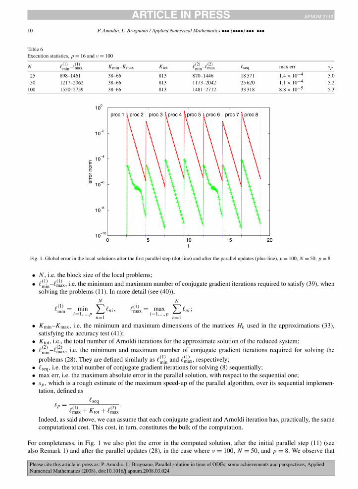
Fig. 1. Global error in the local solutions after the first parallel step (dot-line) and after the parallel updates (plus-line), ν = 100, N = 50, p = 8.

• N , i.e. the block size of the local problems;•

(1)min–

(1)max, i.e. the minimum and maximum number of conjugate gradient iterations required to satisfy (39), when

solving the problems (11). In more detail (see (40)),

(1)min = min

i=1,...,p

N∑n=1

ni, (1)max = max

i=1,...,p

N∑n=1

ni;

• Kmin–Kmax, i.e. the minimum and maximum dimensions of the matrices Hk used in the approximations (33),satisfying the accuracy test (41);

• Ktot, i.e., the total number of Arnoldi iterations for the approximate solution of the reduced system;•

(2)min–

(2)max, i.e. the minimum and maximum number of conjugate gradient iterations required for solving the

problems (28). They are defined similarly as (1)min and

(1)max, respectively;

• seq, i.e. the total number of conjugate gradient iterations for solving (8) sequentially;• max err, i.e. the maximum absolute error in the parallel solution, with respect to the sequential one;• sp , which is a rough estimate of the maximum speed-up of the parallel algorithm, over its sequential implemen-

tation, defined as

sp = seq

(1)max + Ktot +

(2)max

.

Indeed, as said above, we can assume that each conjugate gradient and Arnoldi iteration has, practically, the samecomputational cost. This cost, in turn, constitutes the bulk of the computation.

For completeness, in Fig. 1 we also plot the error in the computed solution, after the initial parallel step (11) (seealso Remark 1) and after the parallel updates (28), in the case where ν = 100, N = 50, and p = 8. We observe that




in the window which concerns the first processor (“proc 1”, in the figure) the error is zero, since on this processor(see Remark 1) the discrete solution is directly computed, as in the sequential algorithm, by solving the system (18).We observe that the “spikes” at the beginning of each window are due to the use of the approximation (33), whoseaccuracy criterion (see (41)) has been chosen in order to obtain the same maximum global error of the sequentialimplementation.

From the obtained results, one has that

(1)min ≈

(2)min, (1)

max ≈ (2)max.

Consequently, it follows that the maximum asymptotic speed-up for the parallel algorithm is p/2. Indeed, it would be(approximately) achieved, provided that the choice of the coarse mesh (2) would result in

Ktot (j)

min = (j)max, j = 1,2.

This is certainly not the case for some of the considered tests (as also confirmed by the column labeled sp in the tables),even though it is a realistic goal, at least for linear and quasi-linear parabolic problems. Moreover, we observe that ineach table the columns labeled Kmin–Kmax and Ktot contain almost exactly the same values. This is a remarkable resultwhich confirms that the sequential section of the algorithm has a cost which is independent of N , as we expect fromthe theory. We would like to emphasize that the maximum asymptotic speed-up p/2 of the algorithm is considerablybetter than that of the “Parareal” algorithm, which cannot exceed p/k∗, if k∗ (� 2) iterations of (24) are needed forits convergence.

5.1. Summary and concluding remarks

In this paper we have recalled the basic facts regarding a parallel method “across the steps” for solving ODE-IVPs.Such method is characterized by the definition of the reduced system (14), whose solution allows to decouple theoriginal problem into p independent sub-problems. Moreover, we have put into evidence the existing connectionswith a subsequent approach, known as “Parareal” algorithm. In fact, the latter is obtained when an iterative solutionof the reduced system (14), induced by a suitable operator splitting, is considered. At last, we propose a straightmodification of the first parallel method, able to cope with problems with large and sparse Jacobians, in particularproblems deriving by the solution, via the method of lines, of linear or quasi-linear parabolic problems. Numericaltests, carried out on a prototype problem, show that the maximum asymptotic speed-up for this approach, when p

parallel processor are used, is p/2.

References

[1] P. Amodio, L. Brugnano, Parallel factorizations and parallel solvers for tridiagonal linear systems, Linear Algebra Appl. 172 (1992) 347–364.[2] P. Amodio, L. Brugnano, The parallel QR factorization algorithm for tridiagonal linear systems, Parallel Computing 21 (1995) 1097–1110.[3] P. Amodio, L. Brugnano, Parallel implementation of block boundary value methods for ODEs, J. Comput. Appl. Math. 78 (1997) 197–211.[4] P. Amodio, L. Brugnano, Parallel ODE solvers based on block BVMs, Adv. Comput. Math. 7 (1997) 5–26.[5] P. Amodio, L. Brugnano, ParalleloGAM: a parallel code for ODEs, Appl. Numer. Math. 28 (1998) 95–106.[6] P. Amodio, I. Gladwell, G. Romanazzi, Numerical solution of general Bordered ABD linear systems by cyclic reduction, J. Numer. Anal. Ind.

Appl. Math. 1 (2006) 5–12.[7] P. Amodio, G. Romanazzi, BABDCR: a Fortran 90 package for the solution of Bordered ABD linear systems, ACM Trans. Math. Software 32

(2006) 597–608.[8] P. Amodio, L. Brugnano, T. Politi, Parallel factorizations for tridiagonal matrices, SIAM J. Numer. Anal. 30 (1993) 813–823.[9] C. Le Bris, Computational chemistry from the perspective of numerical analysis, Acta Numerica 14 (2005) 363–444.

[10] L. Brugnano, D. Trigiante, On the potentiality of sequential and parallel codes based on extended trapezoidal rules (ETRs), Appl. Numer.Math. 25 (1997) 169–184.

[11] L. Brugnano, D. Trigiante, Parallel implementation of block boundary value methods on nonlinear problems: theoretical results, Appl. Numer.Math. 78 (1997) 197–211.

[12] L. Brugnano, D. Trigiante, Solving Differential Problems by Multistep Initial and Boundary Value Methods, Gordon and Breach, Amsterdam,1998.

[13] K. Burrage, Parallel and Sequential Methods for Ordinary Differential Equations, Clarendon Press, Oxford, 1995.[14] K. Burrage (Ed.), Parallel Methods for ODEs, Adv. Comput. Math. 7 (1–2) (1997).[15] M.J. Gander, E. Hairer, Nonlinear convergence analysis for the Parareal algorithm, in: U. Langer, M. Discacciati, D.E. Keyes, O.B. Widlund,

W. Zulehner (Eds.), Domain Decomposition Methods in Science and Engineering XVII, in: Lecture Notes in Computational Science andEngineering, vol. 60, Springer, Berlin, 2008, pp. 45–56.




[16] M.J. Gander, S. Vandewalle, On the superlinear and linear convergence of the Parareal algorithm, in: O.B. Widlund, D.E. Keyes (Eds.),Domain Decomposition Methods in Science and Engineering XVI, in: Lecture Notes in Computational Science and Engineering, vol. 55,Springer, Berlin, 2007, pp. 291–298.

[17] M.J. Gander, S. Vandewalle, Analysis of the Parareal time-parallel time-integration method, SIAM J. Sci. Comput. 29 (2007) 556–578.[18] M. Hochbruck, C. Lubich, On Krylov subspace approximations to the matrix exponential operator, SIAM J. Numer. Anal. 34 (1997) 1911–

1925.[19] J.L. Lions, Y. Maday, G. Turinici, Résolution d’EDP par un schéma en temps “pararéel”, C. R. Acad. Sci. Paris, Ser. I 332 (2001) 661–668.[20] Y. Maday, G. Turinici, A parareal in time procedure for the control of partial differential equations, C. R. Acad. Sci. Paris, Ser. I 335 (2002)

387–392.[21] Y. Maday, G. Turinici, The Parareal in time iterative solver: a further direction to parallel implementation, in: T.J. Barth, M. Griebel,

D.E. Keyes, R.M. Nieminen, D. Roose, T. Schlick, R. Kornhuber, R. Hoppe, J. Périaux, O. Pironneau, O. Widlund, J. Xu (Eds.), DomainDecomposition Methods in Science and Engineering, in: Lecture Notes in Computational Science and Engineering, vol. 40, Springer, Berlin,2005, pp. 441–448.

[22] I. Moret, P. Novati, RD-rational approximations of the matrix exponential, BIT 44 (2004) 595–615.[23] Y. Saad, Analysis of some Krylov subspace approximations to the matrix exponential operator, SIAM J. Numer. Anal. 29 (1992) 209–228.[24] G.A. Staff, The Parareal algorithm. A survey of present work, Report of the Norwegian University of Science and Technology, Dept. of Math.

Sciences, 2003.[25] S. Ulbrich, Generalized SQP-methods with “Parareal” time decomposition for time-dependent PDE-constrained optimization, Technical Re-

port, Fachbereich Mathematik, TU Darmstadt, 2005.


Parallel solution in time of ODEs: some achievements and perspectives

Documents