Parallel Programming - archer.ac.uk · • In effect, parallel programming is required for all computing, not just ... • Or they can be 1-sided – only the sender or receiver is

Parallel Programming Overview and Concepts

Dr Mark Bull, EPCC [email protected]

Outline • Why use parallel programming? • Parallel models for HPC

•  Shared memory (thread-based) •  Message-passing (process-based) •  Other models

• Assessing parallel performance: scaling •  Strong scaling •  Weak scaling

•  Limits to parallelism •  Amdahl’s Law •  Gustafson’s Law

Why use parallel programming? It is harder than serial so why bother?

Drivers for parallel programming •  Traditionally, the driver for parallel programming was that

a single core alone could not provide the time-to-solution required for complex simulations •  Multiple cores were tied together as a HPC machine •  This is the origin of HPC and explains the symbiosis of HPC and

parallel programming

• Recently, due to the physical limits on the increase in power of single cores, the driver is due to the fact that all modern processors are parallel •  In effect, parallel programming is required for all computing, not just

HPC

Focus on HPC •  In HPC, the driver is the same as always

•  Need to run complex simulations with a reasonable time to solution •  Single core or even single/multiple processors in a workstation do

not provide the compute/memory/IO performance required

• Solution is to harness the power of multiple cores/memory/storage simultaneously

•  In order to do this we require concepts to allow us to exploit the resources in a parallel manner •  Hence, parallel programming

• Over time a number of different parallel programming models have emerged.

Parallel models How can we write parallel programs

Shared-memory programming • Shared memory programming is usually based on threads

•  Although some hardware/software allows processes to be programmed as if they share memory

•  Sometimes known as Symmetric Multi-processing (SMP) although this term is now a little old-fashioned

• Most often used for Data Parallelism •  Each thread operates the same set of instructions on a separate

portion of the data

• More difficult to use for Task Parallelism •  Each thread performs a different set of instructions

Shared-memory concepts •  Threads “communicate” by having access to the same

memory space •  Any thread can alter any bit of data •  No explicit communications between the parallel tasks

Advantages and disadvantages • Advantages:

•  Conceptually simple •  Usually minor modifications to existing code •  Often very portable to different architectures

• Disadvantages •  Difficult to implement task-based parallelism – lack of flexibility •  Often does not scale very well •  Requires a large amount of inherent data parallelism (e.g. large

arrays) to be effective •  Can be surprisingly difficult to get good performance

Message-passing programming • Message passing programming is process-based • Processes running simultaneously communicate by

exchanging messages •  Messages can be 2-sided – both sender and receiver are involved

in the process •  Or they can be 1-sided – only the sender or receiver is involved

• Used for both data and task parallelism •  In fact, most message passing programs employ a mixture of data

and task parallelism

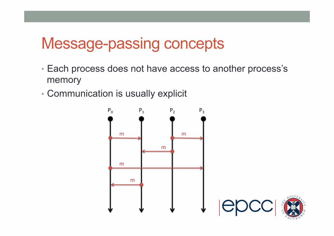
Message-passing concepts • Each process does not have access to another process’s

memory • Communication is usually explicit

Advantages and disadvantages • Advantages:

•  Flexible – almost any parallel algorithm imaginable can be implemented

•  Scaling usually only limited by your choice of algorithm •  Portable – MPI library is provided on all HPC platforms

• Disadvantages •  Parallel routines usually become part of the program due to explicit

nature of communications •  Can be a large task to retrofit into existing code

•  May not give optimum performance on shared-memory machines •  Can be difficult to scale to very large numbers of processes

(>100,000) due to overheads

Scaling Assessing parallel performance

Scaling • Scaling is how the performance of a parallel application

changes as the number of parallel processes/threads is increased

•  There are two different types of scaling: •  Strong Scaling – total problem size stays the same as the number

of parallel elements increases •  Weak Scaling – the problem size increases at the same rate as the

number of parallel elements, keeping the amount of work per element the same

• Strong scaling is generally more useful and more difficult to achieve than weak scaling

Limits to parallel performance How much can you gain from parallelism

Performance improvement •  Two theoretical descriptions of the limits to parallel

performance improvement are useful to consider: •  Amdahl’s Law – how much improvement is possible for a fixed

problem size given more cores

•  Gustafson’s Law – how much improvement is possible given a fixed amount of time and given more cores

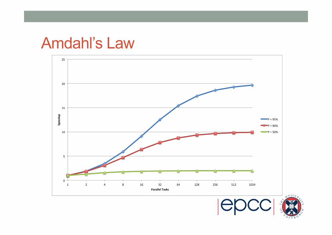
Amdahl’s Law • Performance improvement from parallelisation is strongly

limited by serial portion of the code •  As the serial part’s performance is not increased by adding more

processes/threads •  Based on having a fixed problem size

•  For example, 90% parallelisable (P=0.9): •  S(16) = 6.4 •  S(1024) = 9.9

Amdahl’s Law

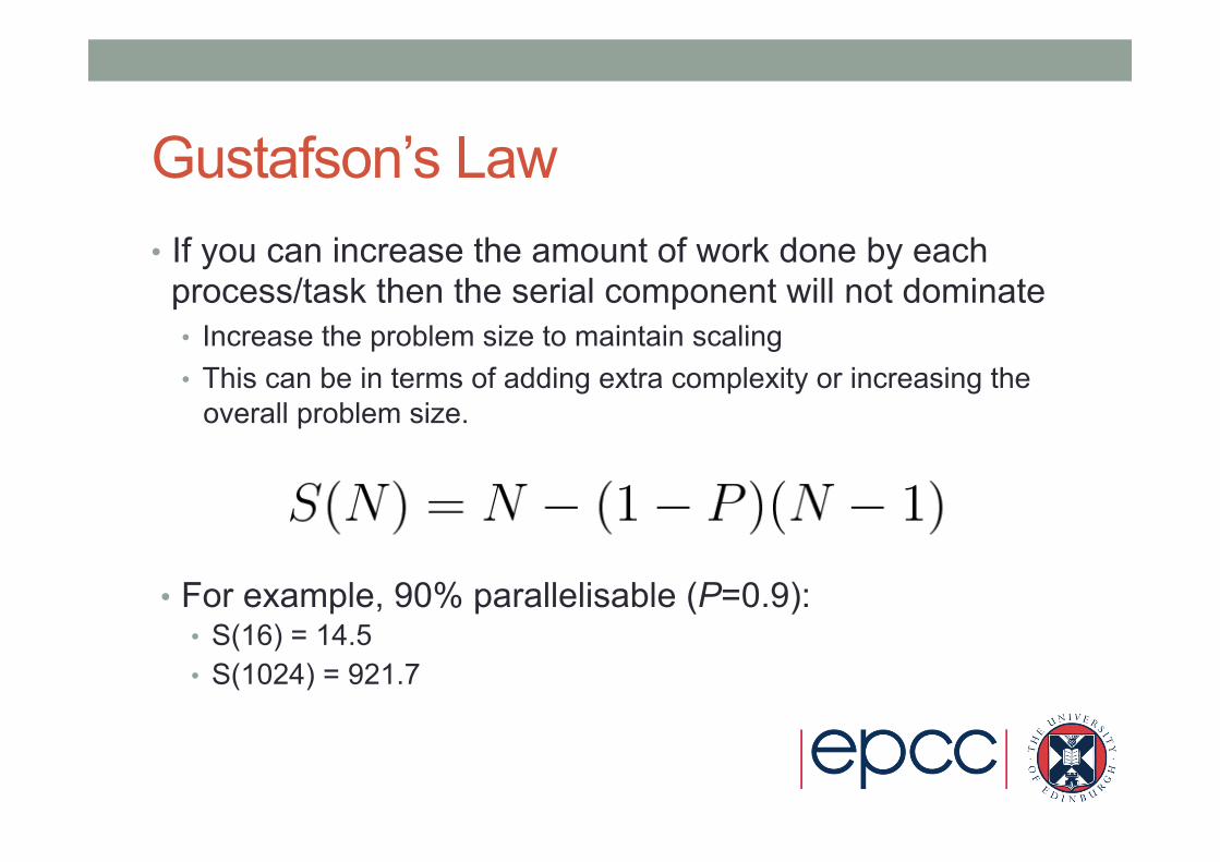
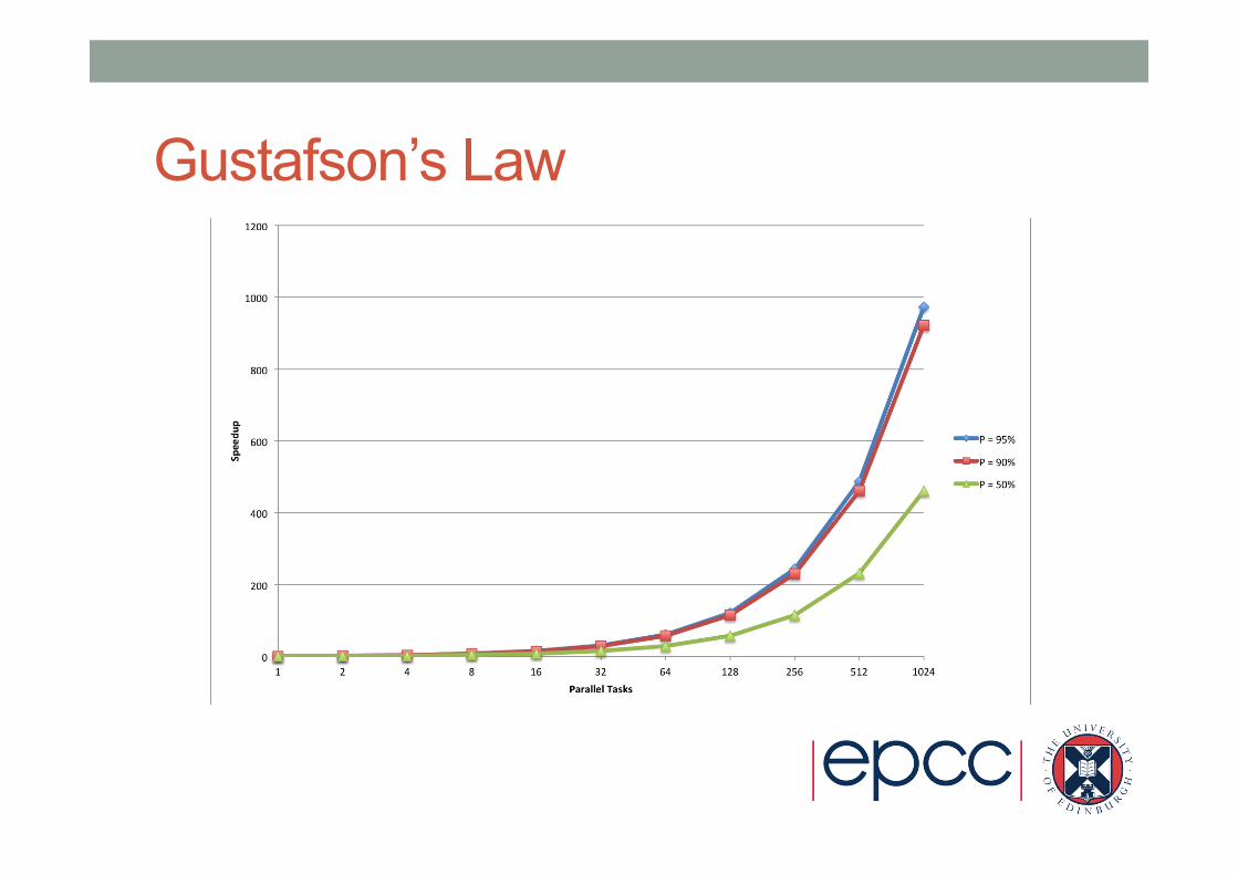
Gustafson’s Law •  If you can increase the amount of work done by each

process/task then the serial component will not dominate •  Increase the problem size to maintain scaling •  This can be in terms of adding extra complexity or increasing the

overall problem size.

•  For example, 90% parallelisable (P=0.9): •  S(16) = 14.5 •  S(1024) = 921.7

Gustafson’s Law

Summary