Parallel implementation of Newton’s method for solving large-scale linear programs

ISSN 0965�5425, Computational Mathematics and Mathematical Physics, 2009, Vol. 49, No. 8, pp. 1303–1317. © Pleiades Publishing, Ltd., 2009.Original Russian Text © V.A. Garanzha, A.I. Golikov, Yu.G. Evtushenko, M.Kh. Nguen, 2009, published in Zhurnal Vychislitel’noi Matematiki i Matematicheskoi Fiziki,2009, Vol. 49, No. 8, pp. 1369–1384.

1303

1. INTRODUCTION

Many applied problems can be reduced to linear problems (LPs), for which numerical methods andsoftware were developed long ago. It may seem that there is not difficult to find an optimal solution in sucha problem. However, the dimension of modern problems (millions of variables and hundreds of thousandsof constraints) is sometimes too large to be solved by conventional methods. Therefore, new approachesare needed for solving such problems on powerful computers.

Large�scale LPs usually have more than one solution. Such techniques as the simplex method, interiorpoint method, or quadratic penalty function method (e.g., see [1, 2]) make it possible to obtain differentsolutions in the case of nonuniqueness. For example, the simplex method yields a solution belonging to avertex of a polyhedron. The interior point method converges to a solution satisfying the strict complemen�tary slackness condition. The method of exterior quadratic penalty function enables one to find the exactnormal solution.

In [3, 4], a new method for solving LPs is proposed that is close to the quadratic penalty functionmethod of the form described in [5, 6] and to the modified Lagrangian function method. When applied tothe dual LP, this method yields the exact projection of the given point on the set of solutions to the primalLP as a result of the one�time unconstrained maximization of an auxiliary piecewise quadratic functionwith a finite penalty coefficient. The use of the generalized Newton method for the maximization of theauxiliary function enables one to solve LPs with a very large number of nonnegative variables (several tensof millions) and a moderate number of constraints (several thousand) on computers based on Pentium�IVprocessors. This paper is devoted to the parallelization of this method so as to make it possible to solve LPswith a larger number of constraints (up to several hundreds of thousands).

In Section 1, we briefly outline the theoretical foundations of the method designed for solving LPs thatenables one to find the projection of the given point on the set of solutions to the primal LP. Using dualitytheory, the auxiliary maximization problem for a concave piecewise quadratic function is obtained inwhich the number of variables is equal to the number of constraints in the primal LP. Formulas for deter�mining the threshold value of the parameter of this function are given; for this threshold, the one�timemaximization of the auxiliary function makes it possible to find the projection of a point on the solutionset of the primal LP using simple formulas. The repeated maximization of the same function in which thesolution of the primal problem is substituted allows one to solve the dual LP.

In Section 2, we recommend to use the generalized Newton method to maximize the auxiliary concavepiecewise quadratic function, which converges in a finite number of steps as shown in [6, 7]. The resultsof solving test LPs on a uniprocessor computer using this method are presented in Section 3. The com�

Parallel Implementation of Newton’s Methodfor Solving Large�Scale Linear Programs

V. A. Garanzha, A. I. Golikov, Yu. G. Evtushenko, and M. Kh. NguenComputing Center, Russian Academy of Sciences, ul. Vavilova 40, Moscow, 119333 Russia

e�mail: [email protected] February 24, 2009

Abstract—Parallel versions of a method based on reducing a linear program (LP) to an unconstrainedmaximization of a concave differentiable piecewise quadratic function are proposed. The maximiza�tion problem is solved using the generalized Newton method. The parallel method is implemented inC using the MPI library for interprocessor data exchange. Computations were performed on the par�allel cluster MVC�6000IM. Large�scale LPs with several millions of variables and several hundreds ofthousands of constraints were solved. Results of uniprocessor and multiprocessor computations arepresented.

DOI: 10.1134/S096554250908003X

Key words: linear programming, generalized Newton’s method, unconstrained optimization, parallelcomputations.

1304

COMPUTATIONAL MATHEMATICS AND MATHEMATICAL PHYSICS Vol. 49 No. 8 2009

GARANZHA et al.

parison of the proposed method (which was implemented in MATLAB) with available commercial andresearch packages showed that it is competitive with the simplex and the interior point methods.

In Section 4, we propose several variants for parallelizing the generalized Newton method as appliedto solving LPs.

In Section 5, we present some numerical results obtained on a parallel cluster. These results show thatthe proposed approach to solving LPs using the generalized Newton method can be efficiently parallelizedand used to solve LPs with several million variables and up to two hundred thousand constraints. Forexample, for LPs with one million variables and 10000 constraints, one of the parallelizing schemes for144 processors of the cluster MVC�6000IM accelerated the computations approximately by a factor of 50,and the computation time was 28 s. A LP with two million variables and 200000 constraints was solved inabout 40 min. on 80 processors.

2. REDUCING LP TO UNCONSTRAINED OPTIMIZATION

Let the LP in normal form

(P)

be given. The dual problem is

(D)

Here, A ∈ �m × n

, c ∈ �n, and b ∈ �

m are given, x is the vector of primal variables, u is the vector of dual

variables, and 0i is the i�dimensional zero vector.Assume that the solution set X* of primal problem (P) is not empty; therefore, the solution set U* of

dual problem (D) is not empty either. We write the Kuhn–Tucker necessary and sufficient conditions forproblems (P) and (D) in the form

(1)

(2)

Here, we introduced the nonnegative vector of slack variables v = c – ATu ≥ 0n in the constraints of dualproblem (D). By D(z), we denote the diagonal matrix in which the ith diagonal entry is the ith componentof the vector z.

Consider the problem of finding the projection of the given point on the solution set X* of primalproblem (P):

(3)

Here and in what follows, we use the Euclidean norm of vectors, and f * is the optimal value of the objec�tive function of the original LP.

For this problem we define the Lagrangian function

Here, p ∈ �m

and β ∈ �1 are the Lagrange multipliers for problem (3). The dual problem for (3) is

(4)

Let us write out the Kuhn–Tucker conditions for problem (3):

(5)

(6)It is easy to verify that conditions (5) are equivalent to the equation

(7)This formula yields a solution of the inner minimization problem in (4).

Substituting (7) in the Lagrangian function L(x, p, β), we obtain the dual function for problem (4):

f* cT

x, Xx X∈min x R

n : Ax = b x 0n≥,∈{ }= =

f* bT

u, Uu U∈max u R

m : A

Tu c≤∈{ }.= =

Ax* b– 0m, x* 0n, D x*( )v*≥ 0n,= =

v* c AT

u*– 0n.≥=

x̂

12�� x̂* x̂–

2 12�� x x̂–

2, X*

x X*∈min x �

n : Ax = b c

Tx = f* x 0n≥, ,∈{ }.= =

L x p β, ,( ) 12�� x x̂–

2p

Tb Ax–( ) β c

Tx f*–( ).+ +=

L x p β, ,( ).x R+

n∈

minβ R

1∈

maxp R

m∈

max

x x̂– AT

p– βc 0n, D x( ) x x̂– AT

p– βc+( )≥+ 0n, x 0n,≥=

Ax b, cT

x f*.= =

x x̂ AT

p βc–+( )+.=

L̂ p β,( ) bT

p 12�� x̂ A

тp βc–+( )+

2

– βf*– 12�� x̂

2.+=


PARALLEL IMPLEMENTATION OF NEWTON’S METHOD 1305

The function (p, β) is concave, piecewise quadratic, and continuously differentiable in its variablesp and β.

Dual problem (4) reduces to the solution of the outer maximization problem

(8)

Solving problem (8), we find the optimizers p and β. Substituting them in (7), we find a solution ofproblem (3), that is, the projection of on the solution set of primal problem (P). The necessary and suf�ficient conditions for (8) are

where x is determined by (7). These conditions are fulfilled if and only if x ∈ X* and x = .Unfortunately, unconstrained optimization problem (8) includes the quantity f *—the optimal value

of the objective function in the original LP—which is not known a priori. However, this problem can besimplified by eliminating this difficulty. For that purpose, we propose to solve the simplified unconstrainedmaximization problem

(9)

where the scalar β is fixed and the function S(p, β) is defined by

(10)

Consider problem (9) and its relationship with primal problem (P). Note that, in distinction from (3),the solution of its dual problem (8) is not unique. Naturally, it is desirable to find among all the solutionsof problem (8) the minimal value β∗ of the Lagrange multiplier β. Then, it follows from Theorem 1 below

that we may fix a β ≥ β∗ in dual problem (8) and maximize the dual function (p, β) only in p; that is, we

can solve problem (9). In this case, the pair [p, β] is a solution of problem (8), and the triple [ , p, β] isa saddle point of problem (3), in which the projection —a solution of (P)—is determined by for�mula (7).

To find the minimal β, we use the Kuhn–Tucker conditions for problem (3), which are necessary andsufficient optimality conditions for this problem. Without loss of generality, assume that the first l compo�nents of are strictly greater than zero. Then, we can represent the vectors , , and c and the matrixA in the form

(11)

where > 0l, = 0d, and d = n – l.

According to decomposition (11), the optimal vector of slack variables v* appearing in the Kuhn–

Tucker conditions (1), (2) for problems (P) and (D) can be represented in the form v*T = [ , ].

Then, by the complementary slackness condition, we have x*Tv* = 0, x* ≥ 0n, v* ≥ 0n, and expression (2)

is written as

(12)

(13)

Using the notation introduced in (11), the necessary and sufficient optimality conditions (5), (6) for prob�lem (3) can be written as

(14)

(15)

(16)

L̂

L̂ p β,( ).β �

1∈

maxp �

m∈

max

x̂*x̂

L̂p p β,( ) b A x̂ Aтp βc–+( )+– b Ax– 0m,= = =

L̂β p β,( ) cT

x̂ Aтp βc–+( )+ f*– c

Tx f*– 0,= = =

x̂*

I S p β,( ),p �

m∈

max=

S p β,( ) bT

p 12�� x̂ A

Tp βc–+( )+

2

.–=

L̂

x̂*x̂*

x̂* x̂* x̂

x̂*T x̂l

*Tx̂d

*T,[ ], x̂T x̂l

T x̂dT,[ ], c

Tcl

Tcd

T,[ ], A Al Ad[ ],= = = =

x̂l* x̂d

*

vl*T

vd*T

vl* cl Al

Tu*– 0l,= =

vd* cd Ad

Tu*– 0d.≥=

x̂l* x̂l Al

Tp βcl–+ 0l,>=

x̂d* 0d, x̂d Ad

Tp βcd–+ 0d,≤=

Alx̂l* b, cl

Tx̂l

* f*.= =

1306


GARANZHA et al.

Among the solutions of system (14)–(16), we find the Lagrange multipliers [p, β] such that β is mini�mal; that is, we have the LP

(17)

The constraints in this problem are consistent; however, the objective function can be unbounded below.In this case, we assume that β∗ = γ, where γ is a certain scalar.

Theorem 1 (see [3, 4]) states that, if the system of equations in (17) has a unique solution with respectto p, then β∗ * can be written in the form

(18)

Here, σ = {l + 1 ≤ i ≤ n : ( )i > 0} is an index set and γ is an arbitrary number.

Theorem 1. Let the solution set X* of problem (P) be not empty. Then, for any β ≥ β∗, where β∗ is defined

by (17), the pair [p(β), β], where p(β) is a solution to unconstrained maximization problem (9) (or, which isthe same, a solution to system A( + ATp – βc)+ = b), determines the projection of the given point onthe solution set X* of primal problem (P) by the formula

(19)

If, in addition, the rank of the matrix Al corresponding to the nonzero components of is m, then β∗ is

found by formula (18) and an exact solution of dual problem (D) is found by solving unconstrained maximi�zation problem (9) by the formula

Theorem 1 allows us to replace problem (8), which involves an a priori unknown number f *, with prob�lem (9), in which this number is replaced by the half�interval [β∗, +∞). The latter problem is considerablysimpler from the computational point of view. Note that β∗ found by solving LP (17) or by formula (18)can be negative.

The next theorem asserts that, if a point x* ∈ X* is known, a solution of dual problem (D) can beobtained by solving (one time) unconstrained maximization problem (9).

Theorem 2. Let the solution set X* of problem (P) be not empty. Then, for any β > 0 and = x* ∈ X*, anexact solution of dual problem (D) is found by the formula u* = p(β)/β, where p(β) is a solution of uncon�strained maximization problem (9).

To illustrate the application of this theorem, consider the exterior quadratic penalty method applied todual problem (D); that is, we consider the problem

(20)

It turns out that an exact solution u* of dual problem (D) can be obtained without letting the penalty coef�ficient β tend to +∞ in (20). If β ≥ β∗ in (20), then, due to Theorem 1, we find the normal solution of

primal problem (P) by formula (19) in which = 0n. According to Theorem 2, the unconstrained maxi�mization problem must then be solved or an arbitrary β > 0:

(21)

Using its solution p(β), we obtain the solution p(β)/β = u* ∈ U* of dual problem (D). Note that the com�plexity of problem (21) does not exceed that of problem (20). Therefore, solving only two unconstrainedmaximization problems, one can obtain the exact projection on the solution set of the primal problem anda solution of the dual problem if one takes β ≥ β∗ in (20) and an arbitrary positive β in (21).

To simultaneously solve the primal and dual LPs, we propose to use the iterative process

(22)

β* β : AlTp βcl = x̂l

*– x̂l– AdT

p βcd– x̂d–≤,{ }p R

m∈

infβ R

1∈

inf .=

β*

x̂d AdT AlAl

T( )1–Al x̂l

* x̂l–( )+( )i

vd*( )

i��, σ

i σ∈max 0≠

γ ∞, σ–> 0.=⎩⎪⎨⎪⎧

=

vd*

x̂ x̂* x̂

x̂* x̂ AT

p β( ) βc–+( )+.=

x̂*

u* 1β�� p β( ) AlAl

T( )1–Al x̂* x̂l–( )–( ).=

x̂

bT

p 12�� A

Tp βc–( )+

2

–⎩ ⎭⎨ ⎬⎧ ⎫

.p �

m∈

max

x̃*

x̂

bT

p 12�� x̃* β A

Tp βc–( )+( )+

2

–⎩ ⎭⎨ ⎬⎧ ⎫

.p �

m∈

max

xs 1+ xs AT

ps 1+ βc–+( )+,=



where the arbitrary parameter β > 0 is fixed and the vector ps + 1 is determined by solving the unconstrainedmaximization problem

(23)

Theorem 3. Let the solution set X* of primal problem (P) be not empty. Then, for any β > 0 and any initialpoint x0, iterative process (22), (23) converges to x* ∈ X* in a finite number of steps ω. The formula u* =pω + 1/β gives an exact solution of dual problem (D).

This iterative process is finite and gives an exact solution of primal problem (P) and an exact solutionof dual problem (D). Note that this method does not require that the threshold value of the penalty coef�ficient be known. However, if the value of this coefficient used in the computations is less than the thresh�old value, the method yields a solution to the primal problem in a finite number of steps rather than theprojection of the initial point on the solution set of the primal LP. Note that x

ω = x* ∈ X* is the projection

of xω – 1 on the solution set X* of problem (P).

2. GENERALIZED NEWTON’S METHOD FOR UNCONSTRAINED MAXIMIZATION OF A PIECEWISE QUADRATIC FUNCTION

Unconstrained maximization problem (23) can be solved using any method, for example, the conju�gate gradient method. However, Mangasarian showed that the generalized Newton method is especiallyefficient for the unconstrained optimization of piecewise quadratic functions (see [7]). A brief descriptionof this method follows.

The function S(p, β, ) to be maximized (see (10)) in problem (9) or in (23) is concave, piecewise qua�dratic, and differentiable. The conventional Hessian for this function does not exist. Indeed, the gradient

of S(p, β, ) is not differentiable. However, we can define a generalized Hessian for this function by

where D#(z) is an n × n diagonal matrix with the ith diagonal entry zi equal to 1 if ( + ATp – βc)i > 0 andto 0 if ( + ATp – βc)i ≤ 0 for i = 1, 2, …, n. The generalized Hessian thus defined is an m × m symmetricnegative semidefinite matrix. Since it can be singular, we use the modified Newton direction

where δ is a small positive number (in the computations, we usually used δ = 10–4) and Im is the identitymatrix of order m.

In this case, the modified Newton method is written as

We used the termination rule

Mangasarian studied the convergence of the generalized Newton method for the unconstrained opti�mization of such a concave piecewise quadratic function with a stepsize chosen using Armijo’s rule. Aproof of the finite global convergence of the generalized Newton method for the unconstrained optimiza�tion of a piecewise quadratic function can be found in [7].

3. COMPUTATIONAL EXPERIMENTS ON A UNIPROCESSOR COMPUTER

We solved randomly generated LPs with a large number of nonnegative variables (up to several mil�lions) and a much smaller number of equality constraints (n � m).

We specified m and n (the number of rows and columns in the matrix A) and the density of filling thematrix with nonzero entries ρ. For example, ρ = 1 implies that all the entries of A were randomly gener�

ps 1+ bT

p 12�� xs A

Tp βc–+( )+

2

–⎩ ⎭⎨ ⎬⎧ ⎫

.p �

m∈

maxarg∈

x̂

∂∂p��S p β x̂, ,( ) b A x̂ A

Tp βc–+( )+–=

x̂

∂2

∂p2

��S p β x̂, ,( ) AD#

z( )AT

,–=

x̂x̂

∂2

∂p2

��S p β x̂, ,( ) δIm–⎝ ⎠⎛ ⎞

1– ∂∂p��S p β x̂, ,( ),–

pk 1+ pk∂2

∂p2

��S pk β x̂, ,( ) δIm–⎝ ⎠⎛ ⎞

1– ∂∂p��S pk β x̂, ,( ).–=

pk 1+ pk– tol.≤

1308


GARANZHA et al.

ated, and, for ρ = 0.01, only 1% of entries were generated and the other entries were set to zero. The entriesof A were randomly chosen in the interval [–50, +50]. The solution x* of primal problem (P) and the solu�tion u* of dual problem (D) were generated as follows. n – 3m components of x* were set to zero, and theothers were randomly chosen in the interval [0, 10]. Half of the components of u* were set to zero, and theothers were randomly chosen in the interval [–10, 10]. The solutions x* and u* were used to find the coef�ficients in the objective function c and the right�hand sides b of LP (P). The vectors b and c were deter�mined by the formulas

if > 0, then ξi = 0; if = 0, then ξi was randomly chosen in the interval

In the results presented below, we assumed that all γi = 1 and θi = 10. Note that, for γi close to zero, ξi =

(c – ATu*)i = ( )i can also be very small. According to formula (18), the a priori unknown quantity β∗can be very large in this case. Then, the generated LP can be difficult to solve.

The proposed method for solving the primal and dual LPs, which combines the use of iterativeprocess (22), (23) and the generalized Newton method, is implemented in MATLAB (see [3, 4]). A2.6 GHz Pentium�IV computer with 1 Gb of memory was used for the computations. Numerical experi�ments with randomly generated LPs showed that the proposed method is very efficient for LPs with a largenumber of nonnegative variables (up 50 million variables) and a moderate number of equality constraints(up to 5 thousand). The time needed to solve such problems was in the range from several tens of secondsto one and a half hour. The high efficiency of these computations is explained by the fact that the majorcomputational effort in the proposed method goes for solving the auxiliary unconstrained maximizationproblem using the generalized Newton method. The dimension of this problem is determined by the num�ber of equality constraints, and this number is considerably less than the number of nonnegative variablesin the original LP.

Table 1 presents the results of the test computations obtained using the program EGM (see [4]), whichimplements method (22), (23) in MATLAB, and other commercial and research packages. All the prob�lems were solved on a 2.02 GHz Celeron computer with 1 Gb of memory. The following packages wereused: BPMPD v. 2.3 (the interior point method, see [8]), MOSEK v. 2.0 (the interior point method, see[9]), and the popular commercial package CPLEX (v. 6.0.1, the interior point and simplex methods).

Table 1 shows the dimensions m and n of the problems, the density ρ of the nonzero entries in thematrix A, the time T needed to solve the LP in seconds, and the number of iterations Iter (for EGM, thetotal number of systems of linear equations that were solved in the Newton method when problem (23)was solved). Everywhere, we assumed that β = 1. The Chebyshev norms of the residual vectors were cal�culated:

(24)

b Ax*, c AT

u* ξ;+= =

xi* xi

*

0 γi ξi θi.≤ ≤ ≤

vd*

∆1 Ax b– ∞, ∆2 AT

u c–( )+ ∞, ∆3 cT

x bT

u– .= = =

Table 1

m × n × ρ Program T, s Iter ∆1 ∆2 ∆3

500 × 104 × 1

EGM (NEWTON) 55.0 12 1.5 × 10–8 1.8 × 10–12 1.2 × 10–7

BPMPD (Interior point) 37.4 23 2.3 × 10–10 1.8 × 10–11 1.1 × 10–10

MOSEK (Interior point) 87.2 6 9.7 × 10–8 3.8 × 10–9 1.6 × 10–6

CPLEX (Interior point) 80.3 11 1.8 × 10–8 1.1 × 10–7 0.0

CPLEX (Simplex) 61.8 8308 8.6 × 10–4 1.9 × 10–10 7.2 × 10–3

3000 × 104 × 0.01

EGM (NEWTON) 155.4 11 6.1 × 10–10 3.4 × 10–13 3.6 × 10–8

BPMPD (Interior point) 223.5 14 4.6 × 10–9 2.9 × 10–10 3.9 × 10–9

MOSEK (Interior point) 42.6 4 3.1 × 10–8 1.2 × 10–8 3.7 × 10–8

CPLEX (Interior point) 69.9 5 1.1 × 10–6 1.3 × 10–7 0.0

CPLEX (Simplex) 1764.9 6904 3.0 × 10–3 8.1 × 10–9 9.3 × 10–2

1000 × (5 × 106) × 0.01 EGM (NEWTON) 1007.5 10 3.9 × 10–8 1.4 × 10–13 6.1 × 10–7

1000 × 105 × 1 EGM (NEWTON) 2660.8 8 2.1 × 10–7 1.4 × 10–12 7.1 × 10–7



The results presented in Table 1 showed that the program EGM for MATLAB is close in terms of effi�ciency to the well�known packages based on the interior point and simplex methods. The third row ofTable 1 shows the results for a LP with five millions of nonnegative variables, 1000 constraints, and 1%density of filling the matrix A by nonzero entries. The computation time of EGM was 16 min. The fourthrow shows the results in the case of 1000 constraints, a completely filled matrix A, and n = 105. The com�putation time in this case was 44 min. Both problems were solved very accurately (the norms of the resid�uals did not exceed 7.1 × 10–7). The other packages failed to solve both problems. Therefore, for large LPs,the program EGM implemented in MATLAB for a uniprocessor computer turned out to be considerablymore efficient than the other packages. Note that an implementation of the same algorithm in C wasapproximately by a factor of eight more efficient in terms of computation time.

In order to increase the number of constraints up to hundreds of thousands, it is reasonable to developa parallel implementation of the proposed method.

4. PARALLEL ITERATIVE ALGORITHMS

We consider parallel implementations of method (22), (23) with the use of the generalized Newtonmethod in the distributed memory model. In this case, each process (program being executed) has anindividual address space and the data exchange between processes is performed using the MPI library. Itis assumed that each process if executed on a separate processor (core).

4.1. Computation Formulas

First, we write out the computation formulas used in the parallel implementation of iterativemethod (22), (23) and the generalized Newton method.

Step 1. Set β > 0, the accuracies for the outer and inner iterations tol1 and tol, respectively, and the ini�tial approximations x0 and p0.

Step 2. Calculate the value of the function

(25)

Here, k is the index of the inner iteration of the Newton method for solving unconstrained maximizationproblem (23) and s is the index of the outer iteration.

Step 3. Calculate the gradient of function (25) with respect to p:

(26)

Step 4. Using the generalized Hessian of function (25), form the matrix Hk ∈ �m × m

:

(27)

Here, the diagonal matrix Dk ∈ �n × n

is specified by

(28)

Step 5. Find the direction of maximization δp by solving the linear system. (29)

using the preconditioned conjugate gradient method. The diagonal part of Hk is used as a preconditioner.Step 6. Determine pk + 1 by the formula

where the iteration parameter τk is found by solving the one�dimensional maximization problem using thebisection or Armijo’s method

.

In practice, in all the computations described below, τk = 1 specified the desired solution of the local max�imization problem so that the search was not required.

Step 7. If the stopping criterion for the inner iterations on k

S pk β xs, ,( ) bT

pk12�� xs A

Tpk βc–+( )+

2

.–=

Gk∂S∂p�� pk β xs, ,( ) b A xs A

Tpk βc–+( )+.–= =

Hk δI ADkAT

.+=

Dk( )ii

1, xs AT

pk βc–+( )i

0>

0, xs AT

pk βc–+( )i � 0.⎩

⎨⎧

=

Hkδp Gk–=

pk 1+ pk τkδp,–=

τk S pk τδp– β xs, ,( )τ

max=

pk 1+ pk– tol≤

1310


GARANZHA et al.

is fulfilled, then set = pk + 1 and find xs + 1 by the formula

(30)

Otherwise, set k = k + 1 and go to Step 2.Step 8. If the stopping criterion for the outer iterations on s

is fulfilled, then find the solution of dual problem (D)

The solution of primal problem (P) is x* = xs + 1. Otherwise, set p0 = , s = s + 1, and go to Step 2.

4.2. Main Operations of the Parallel Algorithm

In algorithm 1–8, the main computationally costly operations are the construction of the system of lin�ear equations (29) and its solution. The parallel implementation of the algorithm requires that the follow�ing main operations be parallelized:

multiplication of a matrix by a vector: Ax and ATp;calculation of scalar products xTy, where x, y ∈ �

n, and pTq, where p, q ∈ �

m;

construction of generalized Hessian (27);multiplication of the generalized Hessian by a vector.Note that all the remaining computations in algorithm 1–8 are local. For example, the conjugate gra�

dient method requires the computation of distributed scalar products and distributed multiplication of amatrix by a vector. The other computations are local and do not require data exchange. For the evaluationof function (25), the distributed multiplication of a matrix by a vector is needed to find the vector

and to find the scalar product bTpk. To calculate gradient (26), one more multiplication of a matrix by avector is needed.

From the viewpoint of the structure of the parallel algorithm, one may assume that an underdetermi�nate linear system with the matrix A is solved using the least squares method because all the major diffi�culties of the parallel algorithm appear already at this stage. Various variants of data decomposition forconstructing parallel algorithms were discussed, for example, in [10, 11].

4.3. Data Decomposition: Column Scheme

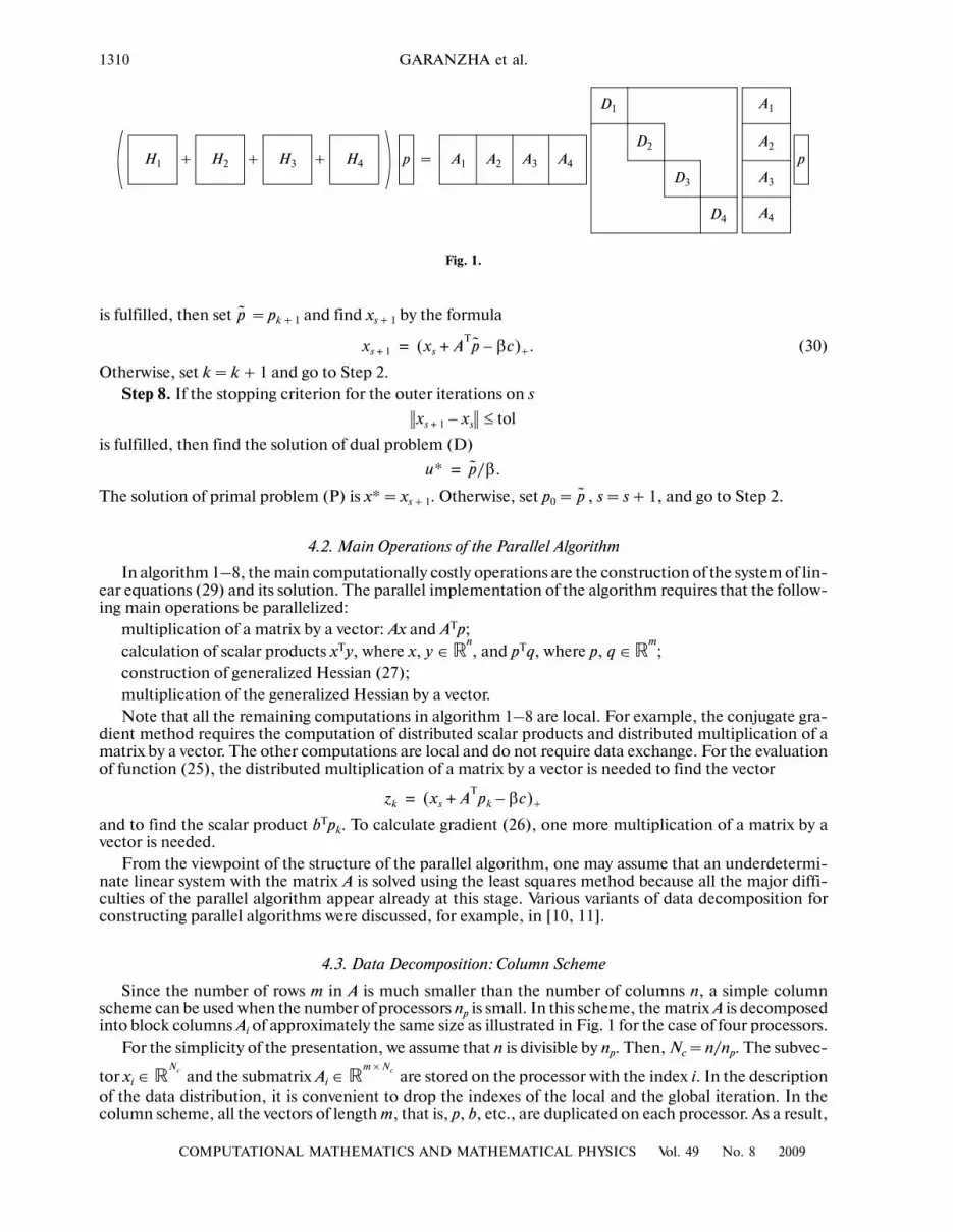
Since the number of rows m in A is much smaller than the number of columns n, a simple columnscheme can be used when the number of processors np is small. In this scheme, the matrix A is decomposedinto block columns Ai of approximately the same size as illustrated in Fig. 1 for the case of four processors.

For the simplicity of the presentation, we assume that n is divisible by np. Then, Nc = n/np. The subvec�

tor xi ∈ and the submatrix Ai ∈ are stored on the processor with the index i. In the descriptionof the data distribution, it is convenient to drop the indexes of the local and the global iteration. In thecolumn scheme, all the vectors of length m, that is, p, b, etc., are duplicated on each processor. As a result,

p̃

xs 1+ xs AT

p̃ βc–+( )+.=

xs 1+ xs– tol≤

u* p̃/β.=

p̃

zk xs AT

pk βc–+( )+=

�Nc

�m Nc×

H1 H2+ + +H3 H4 p A1 A2 A3 A4

D1

D2

D3

D4

A1

A2

A3

A4

p=

Fig. 1.



the multiplication by the transposed matrix, that is, the calculation of the expression ATp is local. On theother hand, the multiplication of A by a vector can be written as

The multiplication of the submatrices by the subvectors xi is performed independently, and the np resultingvectors of length m are added using the function MPI_Allreduce included in the MPI library.

The Hessian H can be written as

where Di ∈ are the diagonal blocks of D. In the column scheme, H is not constructed. The localmatrix Hi is computed on the ith processor. To multiply the matrix by a vector q

,

each component Hiq is calculated locally, and the np resulting vectors are summed up using the functionMPI_Allreduce so that the sum becomes available on all the processors.

As a result, the conjugate gradient method for solving linear system (29) is not parallel, and its compu�tational cost increases proportionally to the number of processors. Denote by γ the ratio of the computa�tional cost of solving the linear system to the other computational costs at a single iteration of the Newtonmethod. Neglecting the time needed to exchange data, we can write an upper bound on the parallelspeedup as

(31)

Therefore, if γ = 0.05, then s(4) = 3.5 and s(6) = 4.85. It is clear that such a simple algorithm is efficientonly when the coefficient γ is sufficiently small.

If the actual communication overheads are taken into account, the speedup can be considerably lower.

4.4. Data Decomposition: Cellular Scheme

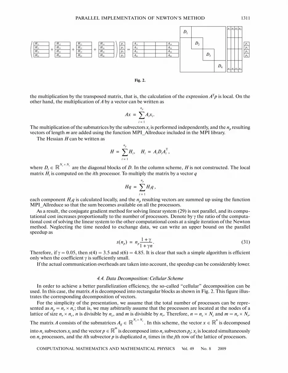
In order to achieve a better parallelization efficiency, the so�called “cellular” decomposition can beused. In this case, the matrix A is decomposed into rectangular blocks as shown in Fig. 2. This figure illus�trates the corresponding decomposition of vectors.

For the simplicity of the presentation, we assume that the total number of processors can be repre�sented as np = nr × nc; that is, we may arbitrarily assume that the processors are located at the nodes of alattice of size nr × nc, n is divisible by nc, and m is divisible by nr. Therefore, n = nc × Nc and m = nr × Nr.

The matrix A consists of the submatrices Aij ∈ . In this scheme, the vector x ∈ �n is decomposed

into nc subvectors xi and the vector p ∈ �m

is decomposed into nr subvectors pj; xi is located simultaneouslyon nr processors, and the ith subvector p is duplicated nc times in the jth row of the lattice of processors.

Ax Aixi.

i 1=

np

∑=

H Hi, Hi

i 1=

np

∑ AiDiAiT

,= =

�Nc Nc×

Hq Hiqi 1=

np

∑=

s np( ) np1 γ+

1 γn+��.=

�Nr Nc×

H11

H21

H31

H41

H12

H22

H32

H42

H13

H23

H33

H43

H14

H24

H34

H44

p1

p2

p3

p4

A11

A21

A31

A41

A14

A24

A34

A44

D1

D2

D3

D4

p1

p2

p3

p4

A11т A21

т A31т A41

т

A14т A24

т A34т A44

т

+ + + =

Fig. 2.

1312


GARANZHA et al.

Consider the main distributed operations for such a decomposition.(a) The operation x = ATp is represented in the form

(32)

At first glance, all the computations are local and, in order to find xi, the sum of nr vectors of length Ncmust be found using, for example, the function MPI_Allreduce included in the MPI library. To find thissum, it is convenient to use the mechanism of splitting the communicators provided by the MPI library.The sums of vectors that reside in different rows of the lattice of processors can be calculated indepen�dently. However, if n is very large, the time spent on data exchange is overly large and no speedup isachieved.

A simple solution is to abandon the optimal computational complexity when multiplying the matrix AT

by a vector. Assume that, for each j, it is known that the jth processor in the ith row of the lattice of pro�cessors contains the entire ith block column of A rather than only the submatrix Aij; that is A is duplicatednr times. If we assume that the vector p is entirely available on each of the nr × nc processors, the same for�mula (32) is independently repeated on all the processors belonging to the same column of the lattice.Therefore, the vector xi is available on all the processors belonging to the ith column of the lattice of pro�cessors without extra exchanges. However, for this purpose, the matrix AT is multiplied by the vector p × nrtimes so that the number of multiplications at this stage is close to ρmnnr.

(b) The operation Ax is almost local because only nc subvectors of length Nr must be added indepen�dently in each of the nr rows of the lattice of processors.

(c) The computations at the stage of forming the matrix H are completely local and require no dataexchange. The number of multiplications at this stage can be estimated as m2ρ2ρzn, where ρz is the fractionof nonzero entries in the diagonal matrix D. In this reasoning, we assumed that the nonzero entries arerandomly distributed over A, that is, the distribution is uniform on the average.

The assembly result is the sum of nc matrices, where the jth summand is distributed over the jth columnof the lattice of processors, as is seen in Fig. 2.

Let the coefficient γhave the same meaning as in formula (31); that is γ is the ratio of the computationalcost of solving the linear system to the other computational costs in a uniprocessor implementation of thealgorithm. The coefficient

(33)

shows an approximate ratio of the cost of multiplying the matrix A by a vector to the cost of forming H ina uniprocessor implementation. Then, we obtain the following very coarse but simple upper bound on thespeedup in the case of using the cellular scheme:

(34)

In practice, the coefficient α is considerably smaller than that given by formula (33). If we set γ = 0.05 andα = 0.1 in (34), then su(8 × 8) = 30.3.

In the analysis of this scheme, we did not consider the question of how to write the whole jth block col�umn of A on every processor in the jth column of the lattice of processors. Indeed, if A is formed locally,that is, if every cell is constructed on one processor, much more time can be needed for such data redistri�bution than for solving the problem. Since, in this study, we formed the matrices using explicit formulas,this question eluded our attention. Note that it is very difficult to construct optimal data structures in thisproblem because the matrix A is very sparse and the Hessian can be assumed to be filled almost completely.

4.5. Data Decomposition: Cyclic Mirror Scheme

In the parallel implementation of the cellular scheme of the decomposition of A, we neglected the factthat the generalized Hessian H is symmetric; therefore the cost of its calculation can be almost halvedcompared with the quadratic matrix of the general form. This cost can be easily reduced in the columnscheme; however, an attempt to do the same in the cellular or row scheme results in a misbalance of theprocessor load both at the stage of constructing H and at the stage of multiplying H by a vector.

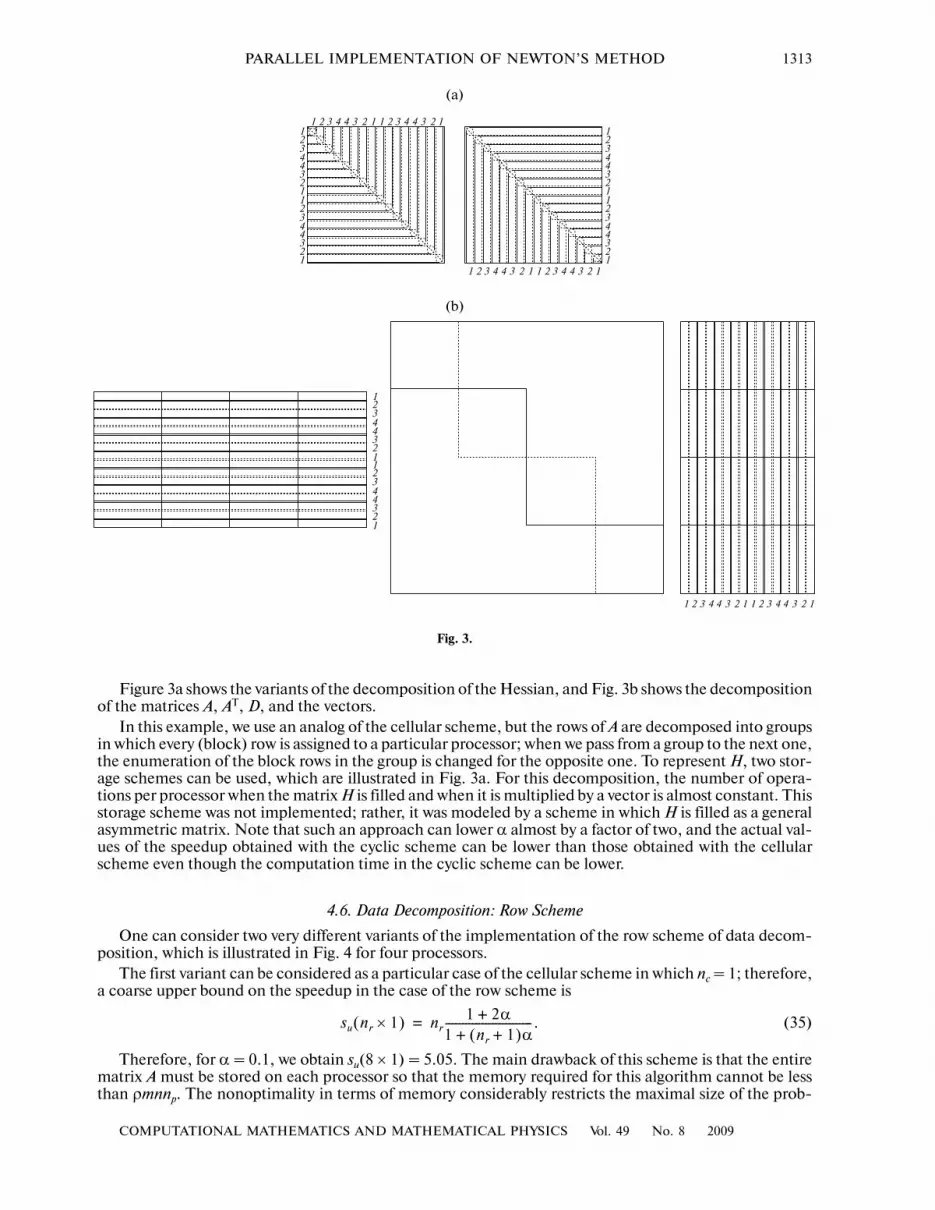
To balance the processor load, the well known cyclic mirror decomposition scheme should be used;this scheme is illustrated in Fig. 3 for the 4 × 4 lattice of processors.

xi AjiT

pj, ij 1=

nr

∑ 1 2 … nc., , ,= =

α ρmn

m2nρ2ρz

�� 1mρρz

��= =

su nr nc×( ) nr1 2α+

1 nr 1+( )α+��nc

1 γ+1 γnc+��.=



Figure 3a shows the variants of the decomposition of the Hessian, and Fig. 3b shows the decompositionof the matrices A, AT, D, and the vectors.

In this example, we use an analog of the cellular scheme, but the rows of A are decomposed into groupsin which every (block) row is assigned to a particular processor; when we pass from a group to the next one,the enumeration of the block rows in the group is changed for the opposite one. To represent H, two stor�age schemes can be used, which are illustrated in Fig. 3a. For this decomposition, the number of opera�tions per processor when the matrix H is filled and when it is multiplied by a vector is almost constant. Thisstorage scheme was not implemented; rather, it was modeled by a scheme in which H is filled as a generalasymmetric matrix. Note that such an approach can lower α almost by a factor of two, and the actual val�ues of the speedup obtained with the cyclic scheme can be lower than those obtained with the cellularscheme even though the computation time in the cyclic scheme can be lower.

4.6. Data Decomposition: Row Scheme

One can consider two very different variants of the implementation of the row scheme of data decom�position, which is illustrated in Fig. 4 for four processors.

The first variant can be considered as a particular case of the cellular scheme in which nc = 1; therefore,a coarse upper bound on the speedup in the case of the row scheme is

(35)

Therefore, for α = 0.1, we obtain su(8 × 1) = 5.05. The main drawback of this scheme is that the entirematrix A must be stored on each processor so that the memory required for this algorithm cannot be lessthan ρmnnp. The nonoptimality in terms of memory considerably restricts the maximal size of the prob�

su nr 1×( ) nr1 2α+

1 nr 1+( )α+��.=

� � � � � � � � � � � � � � � ��

��

� � � � � � � � � � � � � � � �

��

� � � � � � � � � � � � � � � �

(b)

(a)

Fig. 3.

1314


GARANZHA et al.

lems that can be solved. Hence, we face the problem of designing an algorithm that is optimal in terms ofmemory when each processor stores only a block row of A.

We implemented the so�called matrix�free algorithm in which the matrix H is not constructed at all;only its main diagonal is found, and the sequence of operations q = ADATp or

is used to multiply H by the vector p. Here, the vector pj is located at the jth processor. In order to avoidthe exchange of vectors of length n, the sparsity of the diagonal matrix D is used; this property implies that

the number of nonzero components of the vector cannot be greater than in D. Therefore, afterpacking the sparse vectors, the length of the vectors that each processor transmits to its neighbors can beestimated as 2ρzn, which can be considerably less than n.

Unfortunately, at the stage of constructing D, we need the quantity ATp, so that one cannot avoid onesummation of np vectors of length n per each iteration of the Newton method. To optimize this operation,one can use the simultaneous execution of computations and data exchanges. One can hardly expect anefficient parallelization from the matrix�free method. Rather, we would like the parallel version of thealgorithm not to be much slower than the sequential version. Then, the parallel implementation is muchmore efficient than the methods that use virtual memory when the required memory exceeds the avail�able RAM.

On the other hand, if A is a very sparse matrix in the sense that H can also be assumed to be sparse, therow scheme can be very efficient although it must be considerably modified. In addition, in the frameworkof the row scheme, one can efficiently implement the parallel preconditioned conjugate gradient methodfor solving the linear system; as a preconditioner, the reliable incomplete LU factorization can be used asthe preconditioner (see [12]).

5. NUMERICAL RESULTS

For the numerical experiments, we used the generator of random test LPs described in Section 3.The computations were performed on the cluster MVC�6000IM consisting of two�processor nodes

based on 1.6 GHz Intel Itanium 2 processors connected by Myrinet 2000.

qi AjDAjT

pj

j 1=

np

∑=

DAjT

pj

=

H1

H2

H3

H4

p1

p2

p3

p4

A1

A2

A3

A4

D

A1т A2

т A3т A4

т

p1

p2

p3

p4

Fig. 4.

Table 2

T, s snp

1 2 4 8 16 32 64

Ttot 1439.32 1311.40 568.79 408.94 236.68 188.17 142.65

stot 1 1.10 2.53 3.52 6.08 7.65 10.09

Tlin 121.88 124.42 122.09 120.60 116.87 109.80 106.17

slin 1 0.98 1.00 1.01 1.04 1.11 1.15

Trem 1317.35 1186.69 446.61 288.25 119.73 78.30 36.40

srem 1 1.11 2.95 4.57 11.00 16.82 36.19



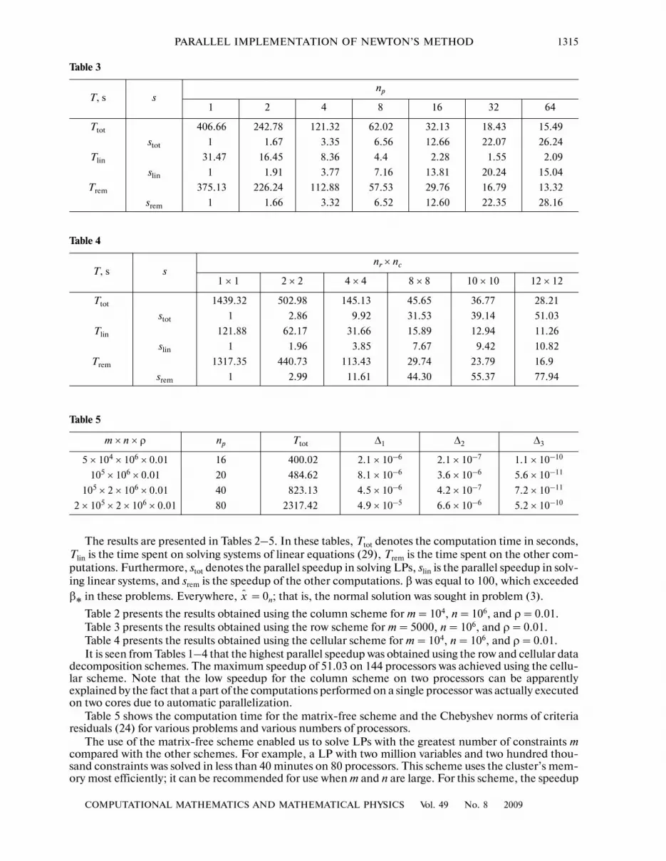
The results are presented in Tables 2–5. In these tables, Ttot denotes the computation time in seconds,Tlin is the time spent on solving systems of linear equations (29), Trem is the time spent on the other com�putations. Furthermore, stot denotes the parallel speedup in solving LPs, slin is the parallel speedup in solv�ing linear systems, and srem is the speedup of the other computations. β was equal to 100, which exceededβ∗ in these problems. Everywhere, = 0n; that is, the normal solution was sought in problem (3).

Table 2 presents the results obtained using the column scheme for m = 104, n = 106, and ρ = 0.01.Table 3 presents the results obtained using the row scheme for m = 5000, n = 106, and ρ = 0.01.Table 4 presents the results obtained using the cellular scheme for m = 104, n = 106, and ρ = 0.01.It is seen from Tables 1–4 that the highest parallel speedup was obtained using the row and cellular data

decomposition schemes. The maximum speedup of 51.03 on 144 processors was achieved using the cellu�lar scheme. Note that the low speedup for the column scheme on two processors can be apparentlyexplained by the fact that a part of the computations performed on a single processor was actually executedon two cores due to automatic parallelization.

Table 5 shows the computation time for the matrix�free scheme and the Chebyshev norms of criteriaresiduals (24) for various problems and various numbers of processors.

The use of the matrix�free scheme enabled us to solve LPs with the greatest number of constraints mcompared with the other schemes. For example, a LP with two million variables and two hundred thou�sand constraints was solved in less than 40 minutes on 80 processors. This scheme uses the cluster’s mem�ory most efficiently; it can be recommended for use when m and n are large. For this scheme, the speedup

x̂

Table 3

T, s snp

1 2 4 8 16 32 64

Ttot 406.66 242.78 121.32 62.02 32.13 18.43 15.49

stot 1 1.67 3.35 6.56 12.66 22.07 26.24

Tlin 31.47 16.45 8.36 4.4 2.28 1.55 2.09

slin 1 1.91 3.77 7.16 13.81 20.24 15.04

Trem 375.13 226.24 112.88 57.53 29.76 16.79 13.32

srem 1 1.66 3.32 6.52 12.60 22.35 28.16

Table 4

T, s snr × nc

1 × 1 2 × 2 4 × 4 8 × 8 10 × 10 12 × 12

Ttot 1439.32 502.98 145.13 45.65 36.77 28.21

stot 1 2.86 9.92 31.53 39.14 51.03

Tlin 121.88 62.17 31.66 15.89 12.94 11.26

slin 1 1.96 3.85 7.67 9.42 10.82

Trem 1317.35 440.73 113.43 29.74 23.79 16.9

srem 1 2.99 11.61 44.30 55.37 77.94

Table 5

m × n × ρ np Ttot ∆1 ∆2 ∆3

5 × 104 × 106 × 0.01 16 400.02 2.1 × 10–6 2.1 × 10–7 1.1 × 10–10

105 × 106 × 0.01 20 484.62 8.1 × 10–6 3.6 × 10–6 5.6 × 10–11

105 × 2 × 106 × 0.01 40 823.13 4.5 × 10–6 4.2 × 10–7 7.2 × 10–11

2 × 105 × 2 × 106 × 0.01 80 2317.42 4.9 × 10–5 6.6 × 10–6 5.2 × 10–10

1316


GARANZHA et al.

for relatively small m can be less than unity. On the other hand, in the most interesting and difficult caseof large m, this scheme is very efficient and sometimes gave the speedup greater than unity. In any case,the matrix�free scheme is much more efficient than the methods that use slow disk memory when the ran�dom access memory is insufficiently large.

The computation time for typical test problems and the speedup for different data decompositionschemes are shown in Fig. 5.

6. CONCLUSIONS AND THE DIRECTIONS OF FURTHER RESEARCH

In this study, parallel versions of the generalized Newton method for solving linear programs based onvarious data distribution schemes (column, row, and cellular schemes) were developed. The resulting par�allel algorithms were successfully used to solve large�scale LPs (up to several millions of variables and sev�eral hundreds of thousands of constraints) for a relatively dense matrix A.

As could be expected, the development of an efficient solver proved to be a very challenging task; forevery parallel variant of the algorithm, a reasonable tradeoff between the computational scalability and thescalability in terms of memory had to be found. The highest speedup was obtained for the cellular scheme.However, depending on the dimension of the problem and the sparsity structure of the matrix A, the cel�lular, row, or column scheme can be optimal.

0 10 20 30 40 50 60 0 10 20 30 40 50 60

0 10 20 30 40 50 60 0 10 20 30 40 50 60

400350300250200150100

50

T, s Computation time for the row scheme m = 5000, n = 1000000, ρ = 0.01

Speedup for the row scheme m = 5000, n = 1000000, ρ = 0.0130

25

20

15

10

5

Computation time for the column scheme m = 10000, n = 1000000, ρ = 0.01

Speedup for the column schemem = 10000, n = 1000000, ρ = 0.01

s

0 20 40 60 80 100 140 0 20 40 60 100 120 140

40353025201510

5

140012001000

800600400200

1400 80Computation time for the cellular schemem = 10000, n = 1000000, ρ = 0.01

Speedup for the cellular scheme m = 10000, n = 1000000, ρ = 0.01

70605040302010

12001000

800600400200

Number of processorsTtot Tlin TremStot Slin Srem

120 80

Fig. 5.



The cost of constructing the generalized Hessian can be considerably reduced by calculating only avariable correction to the Hessian at each iteration of the Newton method.

The resulting speedup is quite acceptable (about 30 for 64 processors); however, it must be taken intoaccount that the parallel assignment of the input data for the solver is a nontrivial task, and it can takelonger time than the parallel solution of the problem.

In the implementation of the parallel algorithm proposed in this paper, shared memory was not used.One can expect that a combination of the algorithms based on a combination of distributed and sharedmemory using MPI/Open MP will produce more efficient algorithms for modern multicore architecturesof computer clusters.

An important factor in the speedup of computations is the optimization of operations on dense andsparse matrices. We used the library Lapack for working with dense matrices. However, the vector andmatrix operations on sparse matrices leave additional possibilities for optimization. In particular, one canuse special representations of sparse matrices that combine portability and make use of the cache memorycharacteristics of modern processors (see [13, 14]); such representations can considerably reduce the timeneeded for vector and matrix multiplications.

ACKNOWLEDGMENTS

This study was supported by the Russian Foundation for Basic Research (project no. 08�01�00619), bythe Program of the State Support of Leading Scientific Schools (project no. NSh�5073.2008.1), and bythe Program P�2 of the Presidium of the Russian Academy of Sciences.

REFERENCES

1. I. I. Eremin, Linear Optimization Theory (Ural’skoe Otdelenie Ross. Akad. Nauk, Yekaterinburg, 1998) [in Rus�sian].

2. F. P. Vasil’ev and A. Yu. Ivanitskii, Linear Programminge (Faktorial, Moscow, 2003) [in Russian].

3. A. I. Golikov and Yu. G. Evtushenko, “Solution Method for Large�Scale Linear Programming Problems,”Dokl. Akad. Nauk 397 (6), 727–732 (2004) [Dokl. Math. 70, 615–619 (2004)].

4. A. I. Golikov, Yu. G. Evtushenko, and N. Mollaverdi, “Application of Newton’s Method for Solving Large Lin�ear Programming Problems,” Zh. Vychisl. Mat. Mat. Fiz. 44, 1564–1573 (2004) [Comput. Math. Math. Phys.44, 1484–1493 (2004)].

5. A. I. Golikov and Yu. G. Evtushenko, “Search for Normal Solutions in Linear Programming Problems,” Zh.Vychisl. Mat. Mat. Fiz. 40, 1766–1786 (2000) [Comput. Math. Math. Phys. 40, 1694–1714 (2000)].

6. C. Kanzow, H. Qi, and L. Qi, “On the Minimum Norm Solution of Linear Programs,” J. Optimizat. TheoryAppl. 116, 333–345 (2003).

7. O. L. Mangasarian, “A Newton Method for Linear Programming,” J. Optimizat. Theory Appl. 121, 1–18(2004).

8. Cs. Meszaros, “The BPMPD Interior Point Solver for Convex Quadratic Programming Problems,” Optimizat.Meth. Software 11, 431–449 (1999).

9. E. D. Andersen and K. D. Andersen, “The MOSEK Interior Point Optimizer for Linear Programming: AnImplementation of Homogeneous Algorithm” in High Performance Optimization (Kluwer, New York, 2000),pp. 197–232.

10. G. Karypis, A. Gupta, and V. Kumar, “A Parallel Formulation of Interior Point Algorithms,” Proc. Supercom�puting, 204–213 (1994).

11. T. F. Coleman, J. Czyzyk, C. Sun, et al., “pPCx: Parallel Software for Linear Programming,” in Proc. EighthSIAM Conf. Parallel Processing for Scientific Computing, PPSC, 1997 (SIAM, 1997).

12. I. E. Kaporin, “High Quality Preconditioning of a General Symmetric Positive Definite Matrix Based on ItsUTU+UTR+RTU�Decomposition,” Numer. Linear Algebra Appl. 5, 483–509 (1998).

13. M. Frigo, C. E. Leiserson, H. Prokop, and S. Ramachandran, “Cache�Oblivious Algorithms,” in Proc. 40thAnn. Symposium on Foundations of Computer Science, New York, 1999, pp. 285–297.

14. G. S. Brodal, “Cache�Oblivious Algorithms and Data Structures,” in Proc. 9th Scandinavian Workshop on Algo�rithm Theory, Lect. Notes Comput. Sci. 3111, (Springer, Berlin, 2004), pp. 3–13.

Parallel implementation of Newton’s method for solving large-scale linear programs

Documents