Parallel Gröbner Basis Algorithms over Finite Fields Christian Eder and Jean-Charles Faugère University of Kaiserslautern October 14, 2016 1 / 50

Welcome message from author
This document is posted to help you gain knowledge. Please leave a comment to let me know what you think about it! Share it to your friends and learn new things together.
Transcript
Parallel Gröbner Basis Algorithms over Finite Fields
Christian Eder and Jean-Charles Faugère
University of Kaiserslautern
October 14, 2016
1 / 50
Table of Contents
1. Gröbner Bases and Buchberger’s Algorithm
2. Faugère’s F4 Algorithm
3. Specialized Linear Algebra for Gröbner Basis Computation
4. GBLA – A Gröbner Basis Linear Algebra Library
5. GB – A Gröbner Basis Library
6. Some benchmarks
7. Outlook
2 / 50

Buchberger’s criterion
S-polynomialsLet f ̸= 0,g ̸= 0 ∈ R and let λ = lcm (lt (f) , lt (g)) be the least common multiple oflt (f) and lt (g). The S-polynomial between f and g is given by
spol (f ,g) ..=λ
lt (f) f −λ
lt (g)g.
Buchberger’s criterion [2]Let I = ⟨f1, . . . , fm⟩ be an ideal in R. A finite subset G ⊂ R is a Gröbner basis for Iif G ⊂ I and for all f ,g ∈ G : spol (f ,g) G−→ 0.
3 / 50

Buchberger’s algorithm
Input: Ideal I = ⟨f1, . . . , fm⟩Output: Gröbner basis G for I1. G← ∅2. G← G ∪ {fi} for all i ∈ {1, . . . ,m}3. Set P← {spol
(fi, fj
)| fi, fj ∈ G, i > j}
4. Choose p ∈ P, P← P \ {p}(a) If p G−→ 0 ▶▶ no new information
Go on with the next element in P.(b) If p G−→ q ̸= 0 ▶▶ new information
Build new S-pair with q and add them to P.Add q to G.Go on with the next element in P.
5. When P = ∅ we are done and G is a Gröbner basis for I.
4 / 50

Buchberger’s algorithm
Input: Ideal I = ⟨f1, . . . , fm⟩Output: Gröbner basis G for I1. G← ∅2. G← G ∪ {fi} for all i ∈ {1, . . . ,m}3. Set P← {spol
(fi, fj
)| fi, fj ∈ G, i > j}
4. Choose p ∈ P, P← P \ {p}
(a) If p G−→ 0 ▶▶ no new informationGo on with the next element in P.
(b) If p G−→ q ̸= 0 ▶▶ new informationBuild new S-pair with q and add them to P.Add q to G.Go on with the next element in P.
5. When P = ∅ we are done and G is a Gröbner basis for I.
4 / 50

Buchberger’s algorithm
Input: Ideal I = ⟨f1, . . . , fm⟩Output: Gröbner basis G for I1. G← ∅2. G← G ∪ {fi} for all i ∈ {1, . . . ,m}3. Set P← {spol
(fi, fj
)| fi, fj ∈ G, i > j}
4. Choose p ∈ P, P← P \ {p}(a) If p G−→ 0 ▶▶ no new information
Go on with the next element in P.(b) If p G−→ q ̸= 0 ▶▶ new information
Build new S-pair with q and add them to P.Add q to G.Go on with the next element in P.
5. When P = ∅ we are done and G is a Gröbner basis for I.
4 / 50
Faugère’s F4 algorithm

Faugère’s F4 algorithm
Input: Ideal I = ⟨f1, . . . , fm⟩Output: Gröbner basis G for I1. G← ∅2. G← G ∪ {fi} for all i ∈ {1, . . . ,m}3. Set P← {(af ,bg) | f ,g ∈ G}4. d← 05. while P ̸= ∅:
(a) d← d+ 1(b) Pd ← Select (P), P← P \ Pd(c) Ld ← {af ,bg | (af ,bg) ∈ Pd}(d) Ld ← Symbolic Preprocessing(Ld,G)(e) Fd ← Reduction(Ld,G)(f) for h ∈ Fd:
▶ If lt (h) /∈ L(G) (all other h are “useless”):▷ P← P ∪ {new pairs with h}▷ G← G ∪ {h}
6. Return G
6 / 50
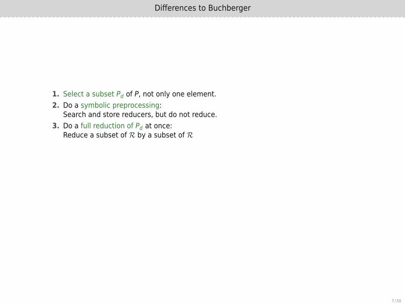
Differences to Buchberger
1. Select a subset Pd of P, not only one element.2. Do a symbolic preprocessing:
Search and store reducers, but do not reduce.3. Do a full reduction of Pd at once:
Reduce a subset of R by a subset of R
If Select (P) selects only one pair F4 is just Buchberger’s algorithm.Usually one chooses the normal selection strategy,
i.e. all pairs of lowest degree.
7 / 50
Symbolic preprocessing
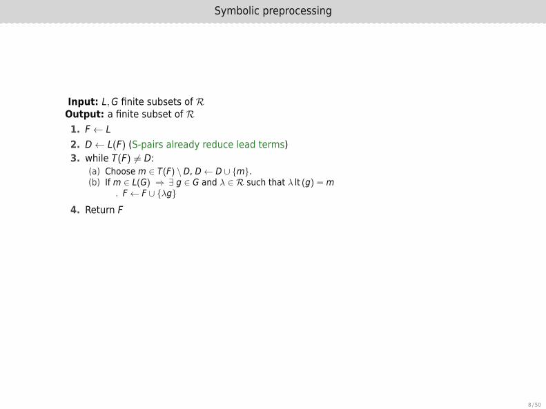
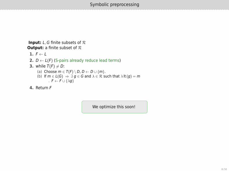
Input: L,G finite subsets of ROutput: a finite subset of R1. F← L2. D← L(F) (S-pairs already reduce lead terms)3. while T(F) ̸= D:
(a) Choose m ∈ T(F) \ D, D← D ∪ {m}.(b) If m ∈ L(G) ⇒ ∃ g ∈ G and λ ∈ R such that λ lt (g) = m
▷ F← F ∪ {λg}
4. Return F
We optimize this soon!
8 / 50
Symbolic preprocessing
Input: L,G finite subsets of ROutput: a finite subset of R1. F← L2. D← L(F) (S-pairs already reduce lead terms)3. while T(F) ̸= D:
(a) Choose m ∈ T(F) \ D, D← D ∪ {m}.(b) If m ∈ L(G) ⇒ ∃ g ∈ G and λ ∈ R such that λ lt (g) = m
▷ F← F ∪ {λg}
4. Return F
We optimize this soon!
8 / 50

Reduction
Input: L finite subsets of ROutput: a finite subset of R1. M← Macaulay matrix of L2. M← Gaussian Elimination of M (Linear algebra)3. F← polynomials from rows of M4. Return F
Macaulay matrix: columns =̂ monomials (sorted by monomial order <)rows =̂ coefficients of polynomials in L
9 / 50

Reduction
Input: L finite subsets of ROutput: a finite subset of R1. M← Macaulay matrix of L2. M← Gaussian Elimination of M (Linear algebra)3. F← polynomials from rows of M4. Return F
Macaulay matrix: columns =̂ monomials (sorted by monomial order <)rows =̂ coefficients of polynomials in L
9 / 50

Example: Cyclic-4
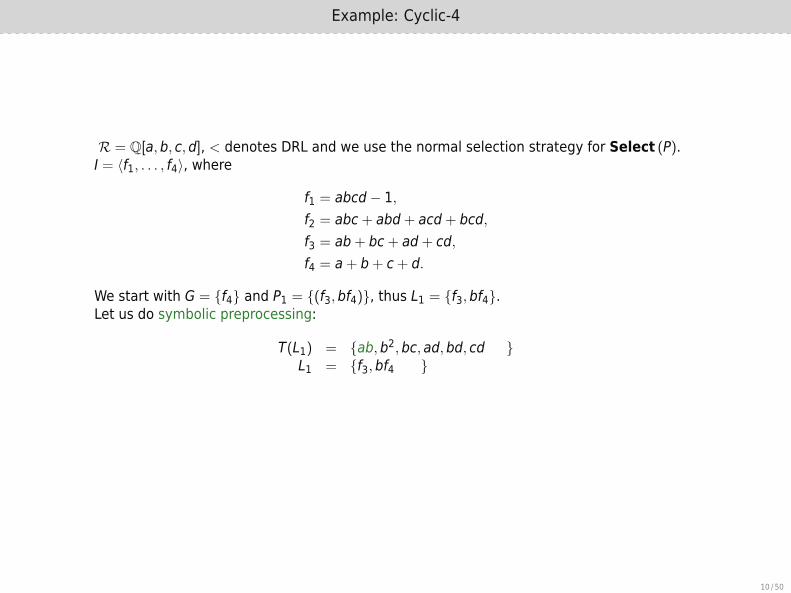
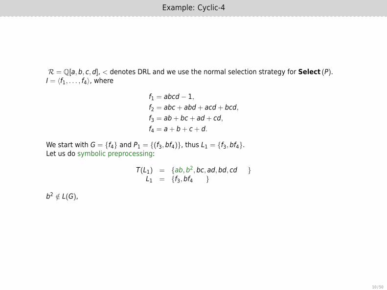
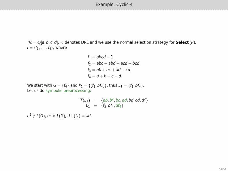
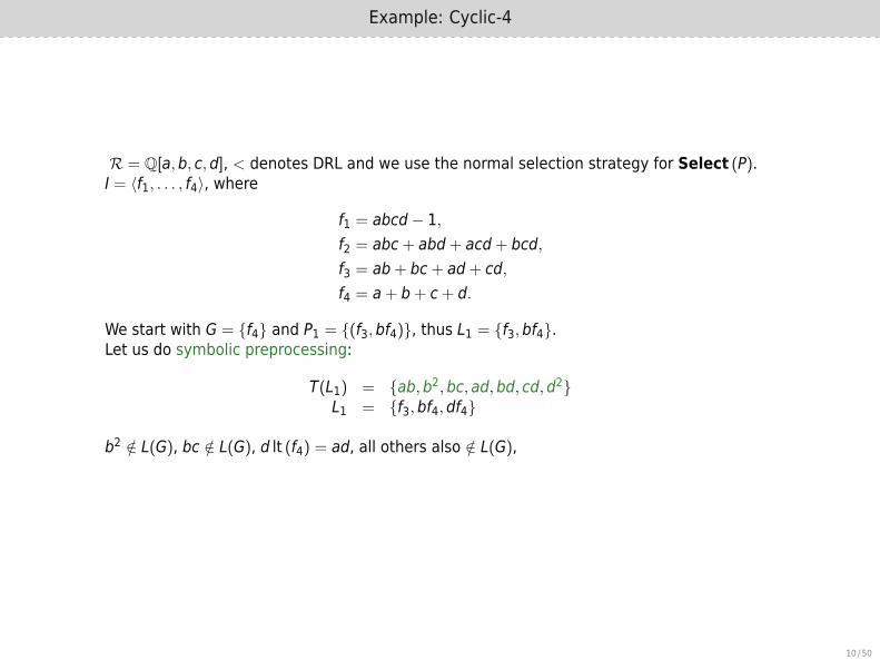
R = Q[a,b, c,d], < denotes DRL and we use the normal selection strategy for Select (P).I = ⟨f1, . . . , f4⟩, where
f1 = abcd− 1,f2 = abc+ abd+ acd+ bcd,f3 = ab+ bc+ ad+ cd,f4 = a+ b+ c+ d.
We start with G = {f4} and P1 = {(f3,bf4)}, thus L1 = {f3,bf4}.Let us do symbolic preprocessing:
T(L1) = {ab,b2,bc, ad,bd, cd
,d2
}L1 = {f3,bf4
,df4
}
b2 /∈ L(G), bc /∈ L(G), d lt (f4) = ad, all others also /∈ L(G),
10 / 50

Example: Cyclic-4
R = Q[a,b, c,d], < denotes DRL and we use the normal selection strategy for Select (P).I = ⟨f1, . . . , f4⟩, where
f1 = abcd− 1,f2 = abc+ abd+ acd+ bcd,f3 = ab+ bc+ ad+ cd,f4 = a+ b+ c+ d.
We start with G = {f4} and P1 = {(f3,bf4)}, thus L1 = {f3,bf4}.
Let us do symbolic preprocessing:
T(L1) = {ab,b2,bc, ad,bd, cd
,d2
}L1 = {f3,bf4
,df4
}
b2 /∈ L(G), bc /∈ L(G), d lt (f4) = ad, all others also /∈ L(G),
10 / 50
Example: Cyclic-4
R = Q[a,b, c,d], < denotes DRL and we use the normal selection strategy for Select (P).I = ⟨f1, . . . , f4⟩, where
f1 = abcd− 1,f2 = abc+ abd+ acd+ bcd,f3 = ab+ bc+ ad+ cd,f4 = a+ b+ c+ d.
We start with G = {f4} and P1 = {(f3,bf4)}, thus L1 = {f3,bf4}.Let us do symbolic preprocessing:
T(L1) = {ab,b2,bc, ad,bd, cd
,d2
}L1 = {f3,bf4
,df4
}
b2 /∈ L(G), bc /∈ L(G), d lt (f4) = ad, all others also /∈ L(G),
10 / 50
Example: Cyclic-4
R = Q[a,b, c,d], < denotes DRL and we use the normal selection strategy for Select (P).I = ⟨f1, . . . , f4⟩, where
f1 = abcd− 1,f2 = abc+ abd+ acd+ bcd,f3 = ab+ bc+ ad+ cd,f4 = a+ b+ c+ d.
We start with G = {f4} and P1 = {(f3,bf4)}, thus L1 = {f3,bf4}.Let us do symbolic preprocessing:
T(L1) = {ab,b2,bc, ad,bd, cd
,d2
}L1 = {f3,bf4
,df4
}
b2 /∈ L(G),
bc /∈ L(G), d lt (f4) = ad, all others also /∈ L(G),
10 / 50

Example: Cyclic-4
R = Q[a,b, c,d], < denotes DRL and we use the normal selection strategy for Select (P).I = ⟨f1, . . . , f4⟩, where
f1 = abcd− 1,f2 = abc+ abd+ acd+ bcd,f3 = ab+ bc+ ad+ cd,f4 = a+ b+ c+ d.
We start with G = {f4} and P1 = {(f3,bf4)}, thus L1 = {f3,bf4}.Let us do symbolic preprocessing:
T(L1) = {ab,b2,bc, ad,bd, cd
,d2
}L1 = {f3,bf4
,df4
}
b2 /∈ L(G), bc /∈ L(G),
d lt (f4) = ad, all others also /∈ L(G),
10 / 50
Example: Cyclic-4
R = Q[a,b, c,d], < denotes DRL and we use the normal selection strategy for Select (P).I = ⟨f1, . . . , f4⟩, where
f1 = abcd− 1,f2 = abc+ abd+ acd+ bcd,f3 = ab+ bc+ ad+ cd,f4 = a+ b+ c+ d.
We start with G = {f4} and P1 = {(f3,bf4)}, thus L1 = {f3,bf4}.Let us do symbolic preprocessing:
T(L1) = {ab,b2,bc, ad,bd, cd,d2}L1 = {f3,bf4,df4}
b2 /∈ L(G), bc /∈ L(G), d lt (f4) = ad,
all others also /∈ L(G),
10 / 50
Example: Cyclic-4
R = Q[a,b, c,d], < denotes DRL and we use the normal selection strategy for Select (P).I = ⟨f1, . . . , f4⟩, where
f1 = abcd− 1,f2 = abc+ abd+ acd+ bcd,f3 = ab+ bc+ ad+ cd,f4 = a+ b+ c+ d.
We start with G = {f4} and P1 = {(f3,bf4)}, thus L1 = {f3,bf4}.Let us do symbolic preprocessing:
T(L1) = {ab,b2,bc, ad,bd, cd,d2}L1 = {f3,bf4,df4}
b2 /∈ L(G), bc /∈ L(G), d lt (f4) = ad, all others also /∈ L(G),
10 / 50
Example: Cyclic-4
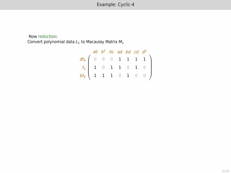
Now reduction:Convert polynomial data L1 to Macaulay Matrix M1
0 0 0 1 1 1 1
1 0 1 1 0 1 0
1 1 1 0 1 0 0
ab b2 bc ad bd cd d2
df4f3
bf4
Gaussian Elimination of M1:
0 0 0 1 1 1 1
1 0 1 0 −1 0 −1
0 1 0 0 2 0 1
ab b2 bc ad bd cd d2
df4f3
bf4
11 / 50

Example: Cyclic-4
Now reduction:Convert polynomial data L1 to Macaulay Matrix M1
0 0 0 1 1 1 1
1 0 1 1 0 1 0
1 1 1 0 1 0 0
ab b2 bc ad bd cd d2
df4f3
bf4
Gaussian Elimination of M1:
0 0 0 1 1 1 1
1 0 1 0 −1 0 −1
0 1 0 0 2 0 1
ab b2 bc ad bd cd d2
df4f3
bf4
11 / 50

Example: Cyclic-4
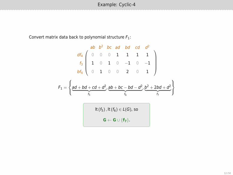
Convert matrix data back to polynomial structure F1:
0 0 0 1 1 1 1
1 0 1 0 −1 0 −1
0 1 0 0 2 0 1
ab b2 bc ad bd cd d2
df4f3
bf4
F1 =
ad+ bd+ cd+ d2︸ ︷︷ ︸f5
, ab+ bc− bd− d2︸ ︷︷ ︸f6
,b2 + 2bd+ d2︸ ︷︷ ︸f7
lt (f5) , lt (f6) ∈ L(G), so
G← G ∪ {f7}.
12 / 50
Example: Cyclic-4
Convert matrix data back to polynomial structure F1:
0 0 0 1 1 1 1
1 0 1 0 −1 0 −1
0 1 0 0 2 0 1
ab b2 bc ad bd cd d2
df4f3
bf4
F1 =
ad+ bd+ cd+ d2︸ ︷︷ ︸f5
, ab+ bc− bd− d2︸ ︷︷ ︸f6
,b2 + 2bd+ d2︸ ︷︷ ︸f7
lt (f5) , lt (f6) ∈ L(G), so
G← G ∪ {f7}.
12 / 50

Example: Cyclic-4
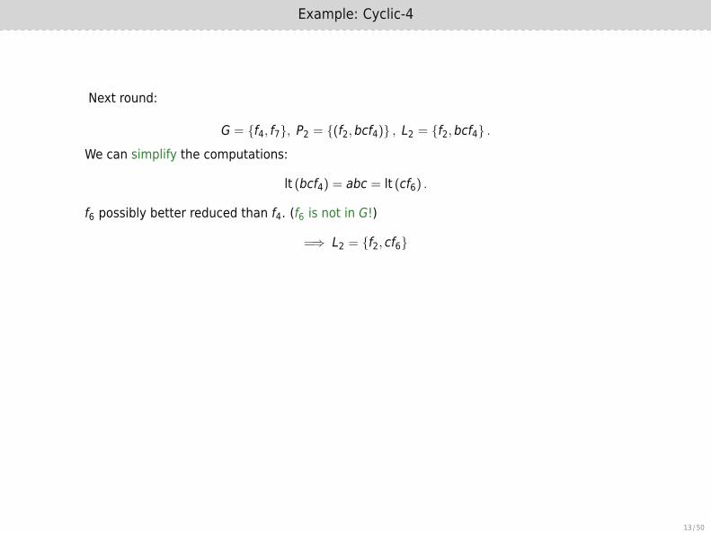
Next round:
G = {f4, f7}, P2 = {(f2,bcf4)} , L2 = {f2,bcf4} .
We can simplify the computations:
lt (bcf4) = abc = lt (cf6) .
f6 possibly better reduced than f4. (f6 is not in G!)
=⇒ L2 = {f2, cf6}
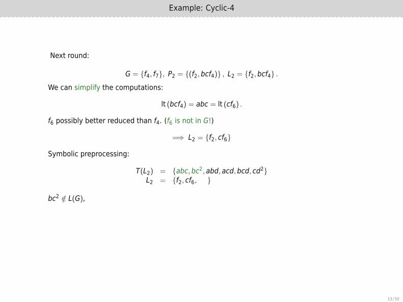
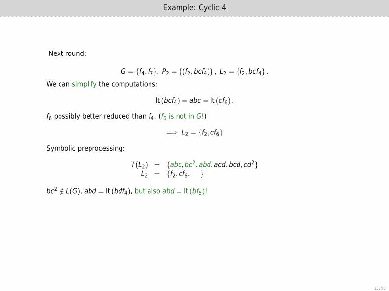
Symbolic preprocessing:
T(L2) = {abc,bc2, abd, acd,bcd, cd2}L2 = {f2, cf6, }
bc2 /∈ L(G), abd = lt (bdf4), but also abd = lt (bf5)!
Let us investigate this in more detail.
13 / 50
Example: Cyclic-4
Next round:
G = {f4, f7}, P2 = {(f2,bcf4)} , L2 = {f2,bcf4} .
We can simplify the computations:
lt (bcf4) = abc = lt (cf6) .
f6 possibly better reduced than f4. (f6 is not in G!)
=⇒ L2 = {f2, cf6}
Symbolic preprocessing:
T(L2) = {abc,bc2, abd, acd,bcd, cd2}L2 = {f2, cf6, }
bc2 /∈ L(G), abd = lt (bdf4), but also abd = lt (bf5)!
Let us investigate this in more detail.
13 / 50
Example: Cyclic-4
Next round:
G = {f4, f7}, P2 = {(f2,bcf4)} , L2 = {f2,bcf4} .
We can simplify the computations:
lt (bcf4) = abc = lt (cf6) .
f6 possibly better reduced than f4. (f6 is not in G!)
=⇒ L2 = {f2, cf6}
Symbolic preprocessing:
T(L2) = {abc,bc2, abd, acd,bcd, cd2}L2 = {f2, cf6, }
bc2 /∈ L(G),
abd = lt (bdf4), but also abd = lt (bf5)!
Let us investigate this in more detail.
13 / 50
Example: Cyclic-4
Next round:
G = {f4, f7}, P2 = {(f2,bcf4)} , L2 = {f2,bcf4} .
We can simplify the computations:
lt (bcf4) = abc = lt (cf6) .
f6 possibly better reduced than f4. (f6 is not in G!)
=⇒ L2 = {f2, cf6}
Symbolic preprocessing:
T(L2) = {abc,bc2, abd, acd,bcd, cd2}L2 = {f2, cf6, }
bc2 /∈ L(G), abd = lt (bdf4), but also abd = lt (bf5)!
Let us investigate this in more detail.
13 / 50

Interlude – Simplify
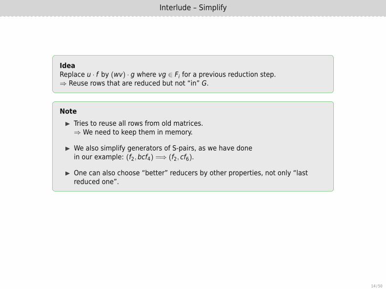
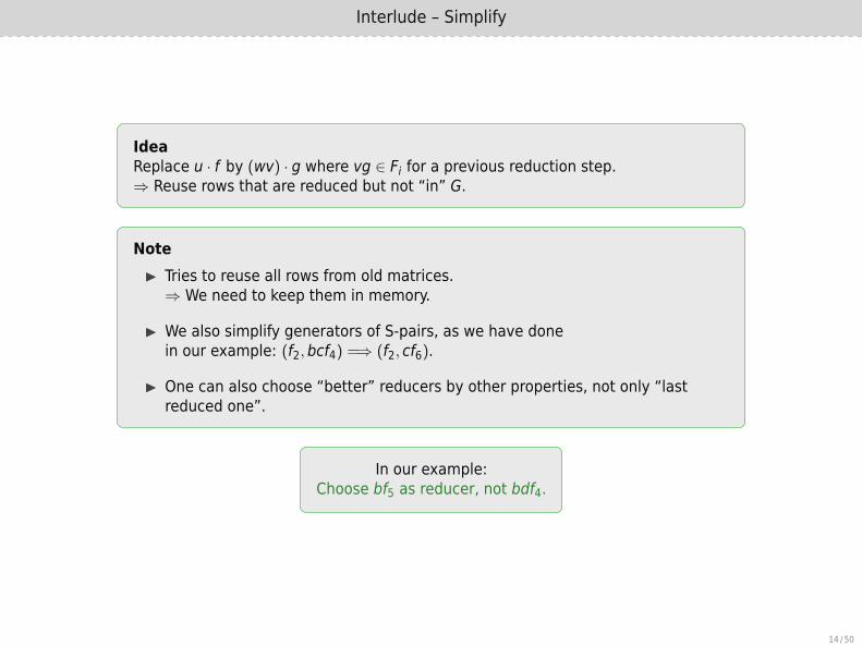
IdeaReplace u · f by (wv) · g where vg ∈ Fi for a previous reduction step.⇒ Reuse rows that are reduced but not “in” G.
Note▶ Tries to reuse all rows from old matrices.⇒ We need to keep them in memory.
▶ We also simplify generators of S-pairs, as we have donein our example: (f2,bcf4) =⇒ (f2, cf6).
▶ One can also choose “better” reducers by other properties, not only “lastreduced one”.
In our example:Choose bf5 as reducer, not bdf4.
14 / 50
Interlude – Simplify
IdeaReplace u · f by (wv) · g where vg ∈ Fi for a previous reduction step.⇒ Reuse rows that are reduced but not “in” G.
Note▶ Tries to reuse all rows from old matrices.⇒ We need to keep them in memory.
▶ We also simplify generators of S-pairs, as we have donein our example: (f2,bcf4) =⇒ (f2, cf6).
▶ One can also choose “better” reducers by other properties, not only “lastreduced one”.
In our example:Choose bf5 as reducer, not bdf4.
14 / 50
Example: Cyclic-4
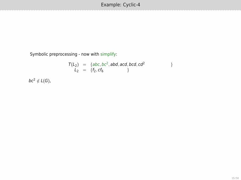
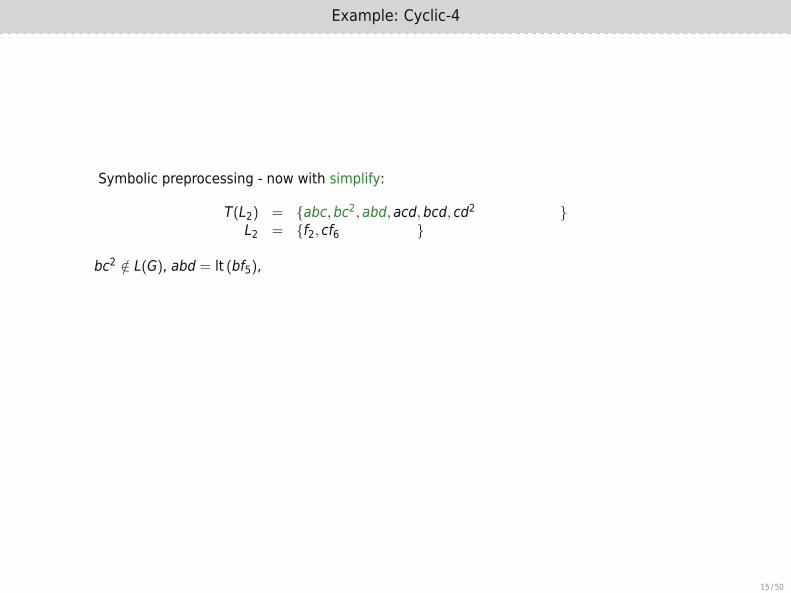
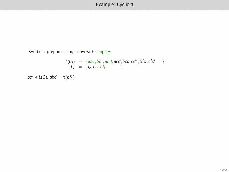
Symbolic preprocessing - now with simplify:
T(L2) = {abc,bc2, abd, acd,bcd, cd2
,b2d, c2d, . . .
}L2 = {f2, cf6
,bf5, cf5,df7
}
bc2 /∈ L(G),
abd = lt (bf5), and so on.
Now try to exploit the special structure of the Macaulay matrices.
15 / 50
Example: Cyclic-4
Symbolic preprocessing - now with simplify:
T(L2) = {abc,bc2, abd, acd,bcd, cd2
,b2d, c2d, . . .
}L2 = {f2, cf6
,bf5, cf5,df7
}
bc2 /∈ L(G), abd = lt (bf5),
and so on.
Now try to exploit the special structure of the Macaulay matrices.
15 / 50
Example: Cyclic-4
Symbolic preprocessing - now with simplify:
T(L2) = {abc,bc2, abd, acd,bcd, cd2,b2d, c2d
, . . .
}L2 = {f2, cf6,bf5
, cf5,df7
}
bc2 /∈ L(G), abd = lt (bf5),
and so on.
Now try to exploit the special structure of the Macaulay matrices.
15 / 50

Example: Cyclic-4
Symbolic preprocessing - now with simplify:
T(L2) = {abc,bc2, abd, acd,bcd, cd2,b2d, c2d, . . . }L2 = {f2, cf6,bf5, cf5,df7}
bc2 /∈ L(G), abd = lt (bf5), and so on.
Now try to exploit the special structure of the Macaulay matrices.
15 / 50

Example: Cyclic-4
Symbolic preprocessing - now with simplify:
T(L2) = {abc,bc2, abd, acd,bcd, cd2,b2d, c2d, . . . }L2 = {f2, cf6,bf5, cf5,df7}
bc2 /∈ L(G), abd = lt (bf5), and so on.
Now try to exploit the special structure of the Macaulay matrices.
15 / 50

Specialized Linear Algebra for Gröbner Basis Computation

Idea by Faugère & Lachartre
Specialize Linear Algebra for reduction steps in GB computations.
1 3 0 0 7 1 01 0 4 1 0 0 50 1 6 0 8 0 10 1 0 0 0 7 00 0 0 0 1 3 1
S-pair
S-pair
reducer
Try to exploit underlying GB structure.
Main ideaDo a static reordering before the Gaussian Elimination to achieve
a better initial shape. Invert the reordering afterwards.
17 / 50

Idea by Faugère & Lachartre
1st step: Sort pivot and non-pivot columns
1 3 0 0 7 1 01 0 4 1 0 0 50 1 6 0 8 0 10 1 0 0 0 7 00 0 0 0 1 3 1
Pivot column Non-Pivot column
1 3 7 0 0 1 01 0 0 4 1 0 50 1 8 6 0 0 90 1 0 0 0 7 00 0 1 0 0 3 1
18 / 50

Idea by Faugère & Lachartre
1st step: Sort pivot and non-pivot columns
1 3 0 0 7 1 01 0 4 1 0 0 50 1 6 0 8 0 10 1 0 0 0 7 00 0 0 0 1 3 1
Pivot column
Non-Pivot column
1 3 7 0 0 1 01 0 0 4 1 0 50 1 8 6 0 0 90 1 0 0 0 7 00 0 1 0 0 3 1
18 / 50

Idea by Faugère & Lachartre
1st step: Sort pivot and non-pivot columns
1 3 0 0 7 1 01 0 4 1 0 0 50 1 6 0 8 0 10 1 0 0 0 7 00 0 0 0 1 3 1
Pivot column
Non-Pivot column
1 3 7 0 0 1 01 0 0 4 1 0 50 1 8 6 0 0 90 1 0 0 0 7 00 0 1 0 0 3 1
18 / 50

Idea by Faugère & Lachartre
1st step: Sort pivot and non-pivot columns
1 3 0 0 7 1 01 0 4 1 0 0 50 1 6 0 8 0 10 1 0 0 0 7 00 0 0 0 1 3 1
Pivot column Non-Pivot column
1 3 7 0 0 1 01 0 0 4 1 0 50 1 8 6 0 0 90 1 0 0 0 7 00 0 1 0 0 3 1
18 / 50

Idea by Faugère & Lachartre
1st step: Sort pivot and non-pivot columns
1 3 0 0 7 1 01 0 4 1 0 0 50 1 6 0 8 0 10 1 0 0 0 7 00 0 0 0 1 3 1
Pivot column Non-Pivot column
1 3 7 0 0 1 01 0 0 4 1 0 50 1 8 6 0 0 90 1 0 0 0 7 00 0 1 0 0 3 1
18 / 50

Idea by Faugère & Lachartre
1st step: Sort pivot and non-pivot columns
1 3 0 0 7 1 01 0 4 1 0 0 50 1 6 0 8 0 10 1 0 0 0 7 00 0 0 0 1 3 1
Pivot column Non-Pivot column
1 3 7 0 0 1 01 0 0 4 1 0 50 1 8 6 0 0 90 1 0 0 0 7 00 0 1 0 0 3 1
18 / 50

Idea by Faugère & Lachartre
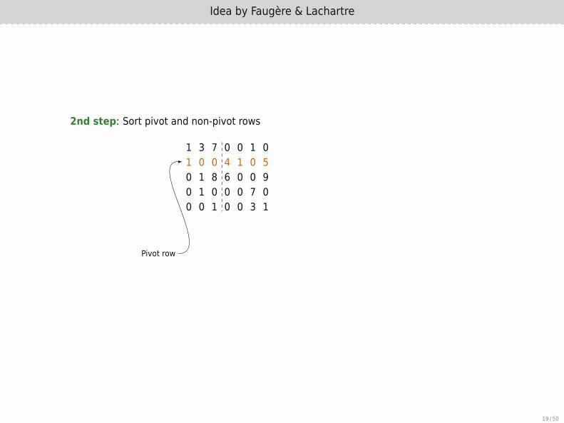
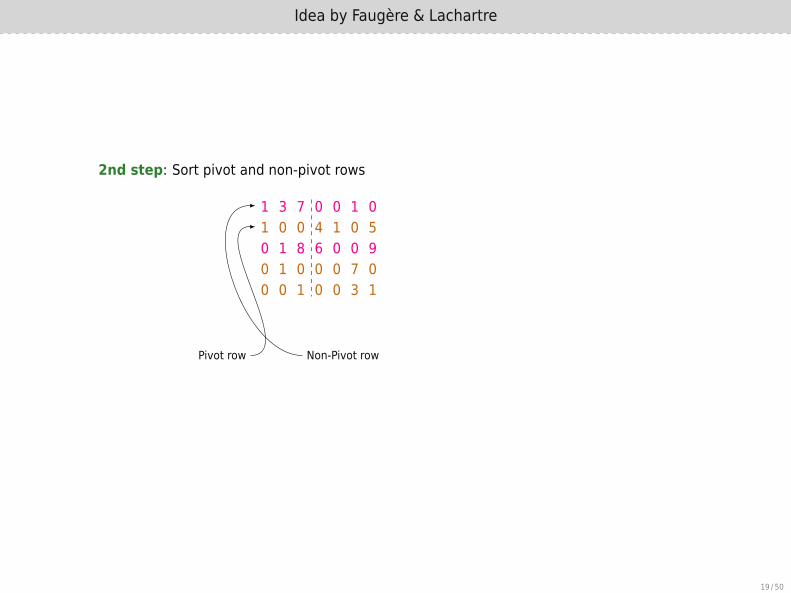
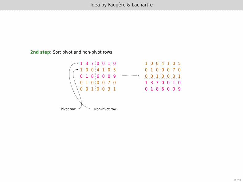
2nd step: Sort pivot and non-pivot rows
1 3 7 0 0 1 01 0 0 4 1 0 50 1 8 6 0 0 90 1 0 0 0 7 00 0 1 0 0 3 1
Pivot row Non-Pivot row
1 0 0 4 1 0 50 1 0 0 0 7 00 0 1 0 0 3 11 3 7 0 0 1 00 1 8 6 0 0 9
19 / 50
Idea by Faugère & Lachartre
2nd step: Sort pivot and non-pivot rows
1 3 7 0 0 1 01 0 0 4 1 0 50 1 8 6 0 0 90 1 0 0 0 7 00 0 1 0 0 3 1
Pivot row
Non-Pivot row
1 0 0 4 1 0 50 1 0 0 0 7 00 0 1 0 0 3 11 3 7 0 0 1 00 1 8 6 0 0 9
19 / 50

Idea by Faugère & Lachartre
2nd step: Sort pivot and non-pivot rows
1 3 7 0 0 1 01 0 0 4 1 0 50 1 8 6 0 0 90 1 0 0 0 7 00 0 1 0 0 3 1
Pivot row Non-Pivot row
1 0 0 4 1 0 50 1 0 0 0 7 00 0 1 0 0 3 11 3 7 0 0 1 00 1 8 6 0 0 9
19 / 50
Idea by Faugère & Lachartre
2nd step: Sort pivot and non-pivot rows
1 3 7 0 0 1 01 0 0 4 1 0 50 1 8 6 0 0 90 1 0 0 0 7 00 0 1 0 0 3 1
Pivot row Non-Pivot row
1 0 0 4 1 0 50 1 0 0 0 7 00 0 1 0 0 3 11 3 7 0 0 1 00 1 8 6 0 0 9
19 / 50
Idea by Faugère & Lachartre
2nd step: Sort pivot and non-pivot rows
1 3 7 0 0 1 01 0 0 4 1 0 50 1 8 6 0 0 90 1 0 0 0 7 00 0 1 0 0 3 1
Pivot row Non-Pivot row
1 0 0 4 1 0 50 1 0 0 0 7 00 0 1 0 0 3 11 3 7 0 0 1 00 1 8 6 0 0 9
19 / 50

Idea by Faugère & Lachartre
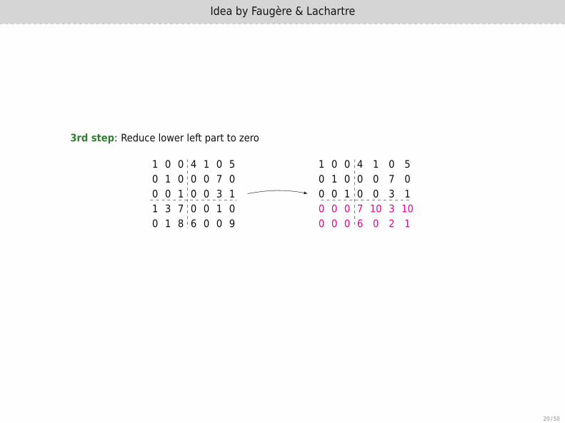
3rd step: Reduce lower left part to zero
1 0 0 4 1 0 50 1 0 0 0 7 00 0 1 0 0 3 11 3 7 0 0 1 00 1 8 6 0 0 9
1 0 0 4 1 0 50 1 0 0 0 7 00 0 1 0 0 3 10 0 0 7 10 3 100 0 0 6 0 2 1
20 / 50
Idea by Faugère & Lachartre
3rd step: Reduce lower left part to zero
1 0 0 4 1 0 50 1 0 0 0 7 00 0 1 0 0 3 11 3 7 0 0 1 00 1 8 6 0 0 9
1 0 0 4 1 0 50 1 0 0 0 7 00 0 1 0 0 3 10 0 0 7 10 3 100 0 0 6 0 2 1
20 / 50

Idea by Faugère & Lachartre
4th step: Reduce lower right part
1 0 0 4 1 0 50 1 0 0 0 7 00 0 1 0 0 3 10 0 0 7 10 3 100 0 0 6 0 2 1
1 0 0 4 1 0 50 1 0 0 0 7 00 0 1 0 0 3 10 0 0 7 0 6 30 0 0 0 4 1 5
5th step: Remap columns and get new polynomials for GB out of lower right part.
21 / 50

Idea by Faugère & Lachartre
4th step: Reduce lower right part
1 0 0 4 1 0 50 1 0 0 0 7 00 0 1 0 0 3 10 0 0 7 10 3 100 0 0 6 0 2 1
1 0 0 4 1 0 50 1 0 0 0 7 00 0 1 0 0 3 10 0 0 7 0 6 30 0 0 0 4 1 5
5th step: Remap columns and get new polynomials for GB out of lower right part.
21 / 50

Idea by Faugère & Lachartre
4th step: Reduce lower right part
1 0 0 4 1 0 50 1 0 0 0 7 00 0 1 0 0 3 10 0 0 7 10 3 100 0 0 6 0 2 1
1 0 0 4 1 0 50 1 0 0 0 7 00 0 1 0 0 3 10 0 0 7 0 6 30 0 0 0 4 1 5
5th step: Remap columns and get new polynomials for GB out of lower right part.
21 / 50

“Real world” matrices?
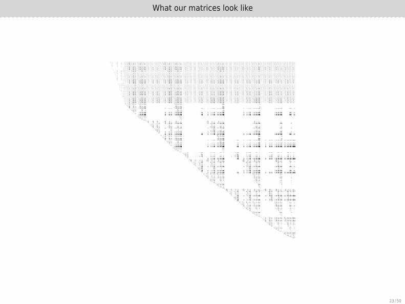
What our matrices look like
23 / 50

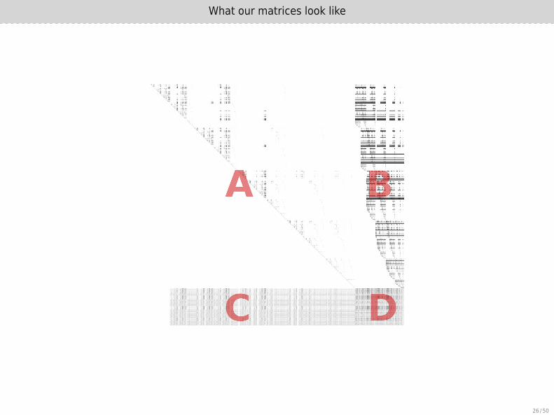
What our matrices look like
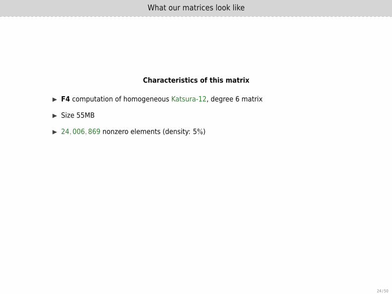
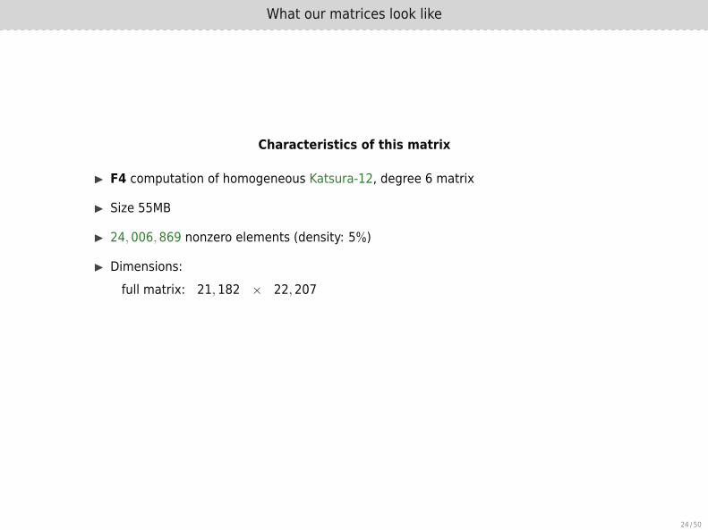
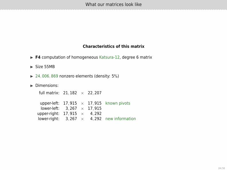
Characteristics of this matrix
▶ F4 computation of homogeneous Katsura-12, degree 6 matrix
▶ Size 55MB
▶ 24,006,869 nonzero elements (density: 5%)
▶ Dimensions:full matrix: 21,182 × 22,207
upper-left: 17,915 × 17,915 known pivotslower-left: 3,267 × 17,915
upper-right: 17,915 × 4,292lower-right: 3,267 × 4,292 new information
24 / 50
What our matrices look like
Characteristics of this matrix
▶ F4 computation of homogeneous Katsura-12, degree 6 matrix
▶ Size 55MB
▶ 24,006,869 nonzero elements (density: 5%)
▶ Dimensions:full matrix: 21,182 × 22,207
upper-left: 17,915 × 17,915 known pivotslower-left: 3,267 × 17,915
upper-right: 17,915 × 4,292lower-right: 3,267 × 4,292 new information
24 / 50

What our matrices look like
25 / 50
What our matrices look like
26 / 50

Hybrid Matrix Multiplication A-1B
27 / 50

Hybrid Matrix Multiplication A-1B
28 / 50

Reduce C to zero
29 / 50

Gaussian Elimination on D
30 / 50

New information
31 / 50

GBLA – A Gröbner Basis Linear Algebra Library

Library Overview
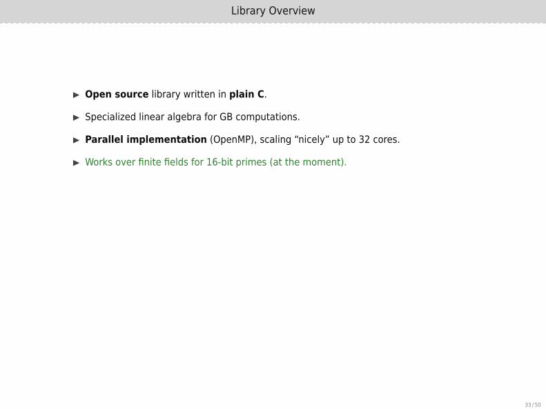
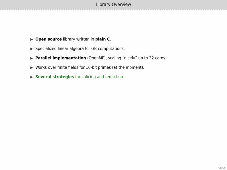
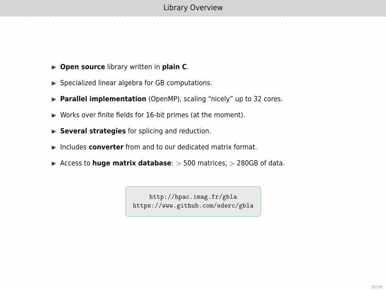
▶ Open source library written in plain C.
▶ Specialized linear algebra for GB computations.
▶ Parallel implementation (OpenMP), scaling “nicely” up to 32 cores.
▶ Works over finite fields for 16-bit primes (at the moment).
▶ Several strategies for splicing and reduction.
▶ Includes converter from and to our dedicated matrix format.
▶ Access to huge matrix database: > 500 matrices, > 280GB of data.
http://hpac.imag.fr/gbla
https://www.github.com/ederc/gbla
33 / 50

Library Overview
▶ Open source library written in plain C.
▶ Specialized linear algebra for GB computations.
▶ Parallel implementation (OpenMP), scaling “nicely” up to 32 cores.
▶ Works over finite fields for 16-bit primes (at the moment).
▶ Several strategies for splicing and reduction.
▶ Includes converter from and to our dedicated matrix format.
▶ Access to huge matrix database: > 500 matrices, > 280GB of data.
http://hpac.imag.fr/gbla
https://www.github.com/ederc/gbla
33 / 50
Exploiting block structures in GB matrices
34 / 50

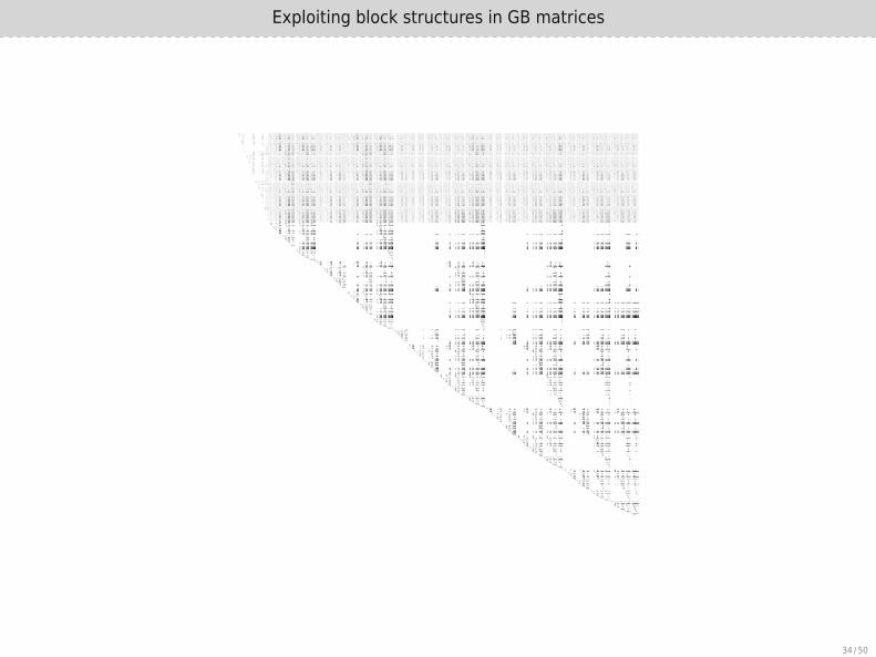
Exploiting block structures in GB matrices
Matrices from GB computations have nonzero entries often grouped in blocks.
Horizontal Pattern If mi,j ̸= 0 then often mi,j+1 ̸= 0.
Vertical Pattern If mi,j ̸= 0 then often mi+1,j ̸= 0.
▶ Can be used to optimize AXPY and TRSM operations in FL reduction.
▶ Horizontal pattern taken care of canonically.
▶ Need to take care of vertical pattern.
35 / 50

Exploiting block structures in GB matrices
Matrices from GB computations have nonzero entries often grouped in blocks.
Horizontal Pattern If mi,j ̸= 0 then often mi,j+1 ̸= 0.Vertical Pattern If mi,j ̸= 0 then often mi+1,j ̸= 0.
▶ Can be used to optimize AXPY and TRSM operations in FL reduction.
▶ Horizontal pattern taken care of canonically.
▶ Need to take care of vertical pattern.
35 / 50

Exploiting block structures in GB matrices
. . . ......
......
......
1 · · · ∗ ∗ ∗ ∗1 · · · ai,j ai,j+1 ∗. . . ...
......
1 · · · ∗1 ∗
1
A......
......
......
...∗ ∗ · · · ∗ · · · ∗ ∗∗ ∗ · · · bi,k ∗ · · · ∗......
......
......
...∗ ∗ · · · bj,k ∗ · · · ∗∗ ∗ · · · bj+1,k ∗ · · · ∗∗ ∗ · · · ∗ · · · ∗ ∗
B
Exploiting horizontal and vertical patterns in the TRSM step.
36 / 50

Multiline data structure – an example
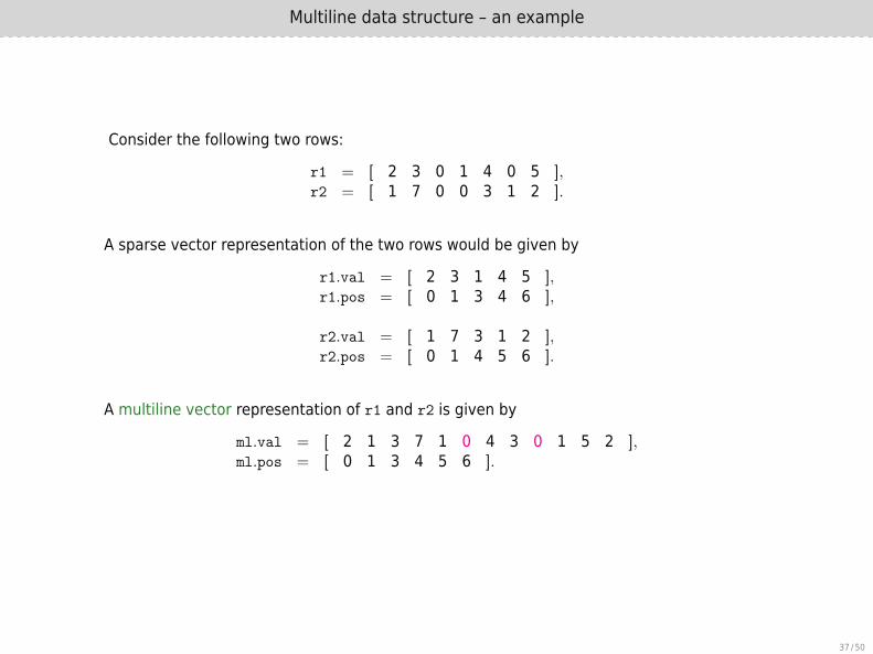
Consider the following two rows:
r1 = [ 2 3 0 1 4 0 5 ],r2 = [ 1 7 0 0 3 1 2 ].
A sparse vector representation of the two rows would be given by
r1.val = [ 2 3 1 4 5 ],r1.pos = [ 0 1 3 4 6 ],
r2.val = [ 1 7 3 1 2 ],r2.pos = [ 0 1 4 5 6 ].
A multiline vector representation of r1 and r2 is given by
ml.val = [ 2 1 3 7 1 0 4 3 0 1 5 2 ],ml.pos = [ 0 1 3 4 5 6 ].
37 / 50

Multiline data structure – an example
Consider the following two rows:
r1 = [ 2 3 0 1 4 0 5 ],r2 = [ 1 7 0 0 3 1 2 ].
A sparse vector representation of the two rows would be given by
r1.val = [ 2 3 1 4 5 ],r1.pos = [ 0 1 3 4 6 ],
r2.val = [ 1 7 3 1 2 ],r2.pos = [ 0 1 4 5 6 ].
A multiline vector representation of r1 and r2 is given by
ml.val = [ 2 1 3 7 1 0 4 3 0 1 5 2 ],ml.pos = [ 0 1 3 4 5 6 ].
37 / 50

New order of operations
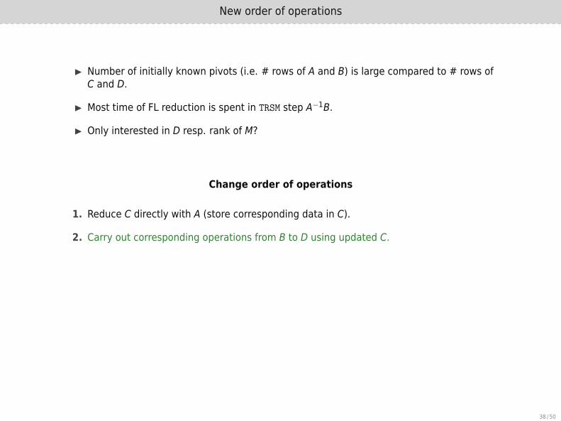
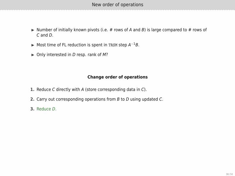
▶ Number of initially known pivots (i.e. # rows of A and B) is large compared to # rows ofC and D.
▶ Most time of FL reduction is spent in TRSM step A−1B.
▶ Only interested in D resp. rank of M?
Change order of operations
1. Reduce C directly with A (store corresponding data in C).
2. Carry out corresponding operations from B to D using updated C.
3. Reduce D.
This leads to reduced matrices that keep A and B untouched,i.e. the computation has a smaller memory footprint.
38 / 50
New order of operations
▶ Number of initially known pivots (i.e. # rows of A and B) is large compared to # rows ofC and D.
▶ Most time of FL reduction is spent in TRSM step A−1B.
▶ Only interested in D resp. rank of M?
Change order of operations
1. Reduce C directly with A (store corresponding data in C).
2. Carry out corresponding operations from B to D using updated C.
3. Reduce D.
This leads to reduced matrices that keep A and B untouched,i.e. the computation has a smaller memory footprint.
38 / 50

GBLA Matrix formats
▶ Matrices are pretty sparse, but structured.
▶ GBLA supports two matrix formats, both use binary format.
▶ GBLA includes a converter between the two supported formats and can also dump toMagma matrix format.
Table: Old matrix format (legacy version)
Size Length Data Descriptionuint32_t 1 b version numberuint32_t 1 m # rowsuint32_t 1 n # columnsuint32_t 1 p prime / field characteristicuint64_t 1 nnz # nonzero entriesuint16_t nnz data entry in matrixuint32_t nnz cols column index of entryuint32_t m rows length of rows
39 / 50

GBLA Matrix formats
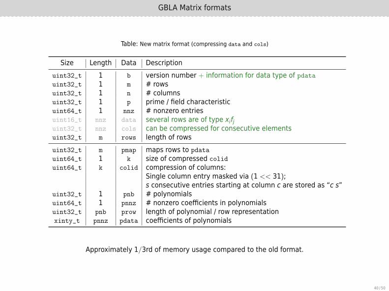
Table: New matrix format (compressing data and cols)
Size Length Data Descriptionuint32_t 1 b version number + information for data type of pdatauint32_t 1 m # rowsuint32_t 1 n # columnsuint32_t 1 p prime / field characteristicuint64_t 1 nnz # nonzero entriesuint16_t nnz data several rows are of type xifjuint32_t nnz cols can be compressed for consecutive elementsuint32_t m rows length of rowsuint32_t m pmap maps rows to pdata
uint64_t 1 k size of compressed colid
uint64_t k colid compression of columns:Single column entry masked via (1 << 31);s consecutive entries starting at column c are stored as “c s”
uint32_t 1 pnb # polynomialsuint64_t 1 pnnz # nonzero coefficients in polynomialsuint32_t pnb prow length of polynomial / row representationxinty_t pnnz pdata coefficients of polynomials
Approximately 1/3rd of memory usage compared to the old format.
40 / 50
GBLA Matrix formats
Table: New matrix format (compressing data and cols)
Size Length Data Descriptionuint32_t 1 b version number + information for data type of pdatauint32_t 1 m # rowsuint32_t 1 n # columnsuint32_t 1 p prime / field characteristicuint64_t 1 nnz # nonzero entriesuint16_t nnz data several rows are of type xifjuint32_t nnz cols can be compressed for consecutive elementsuint32_t m rows length of rowsuint32_t m pmap maps rows to pdata
uint64_t 1 k size of compressed colid
uint64_t k colid compression of columns:Single column entry masked via (1 << 31);s consecutive entries starting at column c are stored as “c s”
uint32_t 1 pnb # polynomialsuint64_t 1 pnnz # nonzero coefficients in polynomialsuint32_t pnb prow length of polynomial / row representationxinty_t pnnz pdata coefficients of polynomials
Approximately 1/3rd of memory usage compared to the old format.
40 / 50

GBLA Matrix formats – Comparison
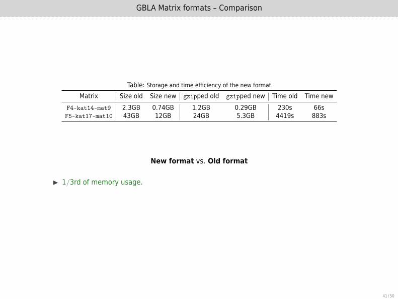
Table: Storage and time efficiency of the new formatMatrix Size old Size new gzipped old gzipped new Time old Time new
F4-kat14-mat9 2.3GB 0.74GB 1.2GB 0.29GB 230s 66sF5-kat17-mat10 43GB 12GB 24GB 5.3GB 4419s 883s
New format vs. Old format
▶ 1/3rd of memory usage.
▶ 1/4th of memory usage when compressed with gzip.
▶ Compression 4− 5 times faster.
41 / 50

GBLA Matrix formats – Comparison
Table: Storage and time efficiency of the new formatMatrix Size old Size new gzipped old gzipped new Time old Time new
F4-kat14-mat9 2.3GB 0.74GB 1.2GB 0.29GB 230s 66sF5-kat17-mat10 43GB 12GB 24GB 5.3GB 4419s 883s
New format vs. Old format
▶ 1/3rd of memory usage.
▶ 1/4th of memory usage when compressed with gzip.
▶ Compression 4− 5 times faster.
41 / 50

GB – A Gröbner Basis Library

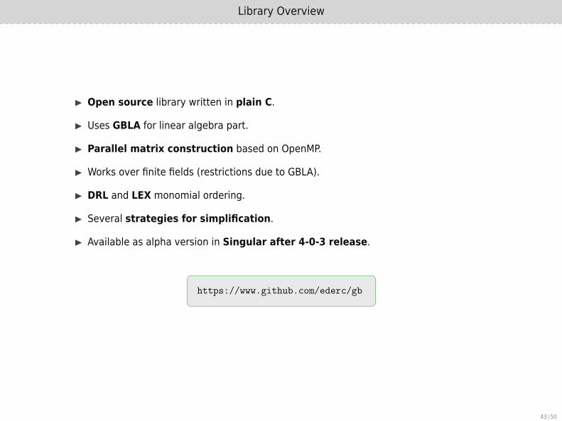
Library Overview
▶ Open source library written in plain C.
▶ Uses GBLA for linear algebra part.
▶ Parallel matrix construction based on OpenMP.
▶ Works over finite fields (restrictions due to GBLA).
▶ DRL and LEX monomial ordering.
▶ Several strategies for simplification.
▶ Available as alpha version in Singular after 4-0-3 release.
https://www.github.com/ederc/gb
43 / 50

Katsura–n w.r.t. DRL (single-threaded)
n
Time (log 2) in seconds
12 13 14 150
2
4
6
8
10
12
14
16
Singular 4-0-3FGb v1.68GB v0.1 w/ GBLA v0.2
44 / 50

Cyclic–n w.r.t. DRL (single-threaded)
n
Time (log 2) in seconds
7 8 9 100
2
4
6
8
10
12
14
16
Singular 4-0-3FGb v1.68GB v0.1 w/ GBLA v0.2
Magma v2.21 / Maple 2016
45 / 50

Cyclic–n w.r.t. DRL (single-threaded)
n
Time (log 2) in seconds
7 8 9 100
2
4
6
8
10
12
14
16
Singular 4-0-3FGb v1.68GB v0.1 w/ GBLA v0.2Magma v2.21 / Maple 2016
45 / 50

Cyclic–10 w.r.t. DRL (n-threads)
n
Time (log 2) in seconds
1 2 4 8 120
2
4
6
8
10
12
14
16
GB v0.1 w/ GBLA v0.2Maple 2016
46 / 50

Next steps
▶ v0.3 of GBLA.
▶ Optimizing GBLA for floating point and 32-bit unsigned int arithmetic.
▶ Multi-modular computation in GB.
▶ Parallel hashing in GB.
▶ Better handling of memory bounds in GB/GBLA.
▶ FGLM in GB for zero-dimensional system solving.
▶ First steps exploiting heterogeneous CPU/GPU platforms for GBLA.
▶ Deeper investigation on parallelization on networks.
47 / 50

References
[1] Boyer, B. and Eder, C. and Faugère, J.-C. and Lachartre, S. and Martani, F. GBLA -Gröbner Basis Linear Algebra Package, 2016. Proceedings of the 2016 InternationalSymposium on Symbolic and Algebraic Computation
[2] Buchberger, B. Ein Algorithmus zum Auffinden der Basiselemente desRestklassenringes nach einem nulldimensionalen Polynomideal, 1965. PhD thesis,Universtiy of Innsbruck, Austria
[3] Buchberger, B. A criterion for detecting unnecessary reductions in the construction ofGröbner bases, 1979. EUROSAM ’79, An International Symposium on Symbolic andAlgebraic Manipulation
[4] Buchberger, B. Gröbner Bases: An Algorithmic Method in Polynomial Ideal Theory,1985. Multidimensional Systems Theory, D. Reidel Publication Company
[5] Eder, C. and Faugère, J.-C. A survey on signature-based Gröbner basis algorithms,2016. Journal of Symbolic Computation
[6] Faugère, J.-C. A new efficient algorithm for computing Gröbner bases (F4), 1999.Journal of Pure and Applied Algebra
[7] Faugère, J.-C. A new efficient algorithm for computing Gröbner bases without reductionto zero (F5), 2002. Proceedings of the 2002 International Symposium on Symbolic andAlgebraic Computation
[8] Faugère, J.-C. and Lachartre, S. Parallel Gaussian Elimination for Gröbner basescomputations in finite fields, 2010. Proceedings of the 4th International Workshop onParallel and Symbolic Computation
[9] Gebauer, R. and Möller, H. M. On an installation of Buchberger’s algorithm, 1988.Journal of Symbolic Computation
48 / 50

Thank you!

Questions? Comments?
Related Documents


![arXiv:1701.06248v1 [cs.SC] 23 Jan 2017 · 2018. 8. 31. · arXiv:1701.06248v1 [cs.SC] 23 Jan 2017 Criteria for Finite Difference Gröbner Bases of Normal Binomial Difference Ideals∗](https://static.cupdf.com/doc/110x72/5fc5adc80e42145195662f19/arxiv170106248v1-cssc-23-jan-2017-2018-8-31-arxiv170106248v1-cssc.jpg)