SpringSim’20, May 19-May 21, 2020, Fairfax, VA, USA; ©2020 Society for Modeling & Simulation International (SCS) PARALLEL EXECUTION OF DEVS IN SHARED-MEMORY MULTICORE ARCHITECTURES Juan Lanuza Guillermo G. Trabes Faculty of Natural and Exact Sciences University of Buenos Aires Department of Systems and Computer Engineering, Carleton University and Intendente Güiraldes 2160 Universidad Nacional de San Luis Buenos Aires, C1428, ARGENTINA 1125 Colonel By Dr. [email protected] Ottawa, ON K1S 5B6, CANADA [email protected] Gabriel Wainer Department of Systems and Computer Engineering, Carleton University 1125 Colonel By Dr. Ottawa, ON K1S 5B6, CANADA [email protected] ABSTRACT Complex models in science and engineering need better techniques to execute simulations efficiently. The Discrete-Event System Specification (DEVS) formalism, a well-known technique for modeling and simula- tion, has been enhanced by executing in parallel computers. Here, we present the design and implemen- tation of a parallel version of the Cadmium DEVS simulator. We conducted empirical evaluation for exe- cuting the protocol in multithreading architectures and discuss performance by applying these techniques in real problems. Keywords: DEVS, parallel simulation, concurrency 1 INTRODUCTION Discrete Event System Specification (DEVS) (Zeigler et al. 2000) is a well-known formalism for modeling and simulation where models are described in a hierarchical and modular manner. DEVS has been used for modeling and simulations of systems in multiple fields of study and there has been a growing demand to simulate complex models, leading to increasing execution times. There have been multiple attempts to achieve parallel executions of DEVS using parallel discrete-event simulation approaches, but, in practice, the resulting simulation architectures end up being very complex and several issues arise related to zero lookahead loops and correctness, in the sense that the correct result for the simulation cannot be achieved in every situation. In (Zeigler 2017), the authors introduce a simple high-level DEVS simulation protocol with parallel execu- tion was presented, allowing multiple simultaneous transitions in the model to execute in parallel, while

Welcome message from author
This document is posted to help you gain knowledge. Please leave a comment to let me know what you think about it! Share it to your friends and learn new things together.
Transcript

SpringSim’20, May 19-May 21, 2020, Fairfax, VA, USA; ©2020 Society for Modeling & Simulation International (SCS)
PARALLEL EXECUTION OF DEVS IN SHARED-MEMORY MULTICORE ARCHITECTURES
Juan Lanuza
Guillermo G. Trabes
Faculty of Natural and Exact Sciences
University of Buenos Aires
Department of Systems and Computer
Engineering, Carleton University and
Intendente Güiraldes 2160 Universidad Nacional de San Luis
Buenos Aires, C1428, ARGENTINA 1125 Colonel By Dr.
[email protected] Ottawa, ON K1S 5B6, CANADA
Gabriel Wainer
Department of Systems and Computer
Engineering, Carleton University
1125 Colonel By Dr.
Ottawa, ON K1S 5B6, CANADA
ABSTRACT
Complex models in science and engineering need better techniques to execute simulations efficiently. The
Discrete-Event System Specification (DEVS) formalism, a well-known technique for modeling and simula-
tion, has been enhanced by executing in parallel computers. Here, we present the design and implemen-
tation of a parallel version of the Cadmium DEVS simulator. We conducted empirical evaluation for exe-
cuting the protocol in multithreading architectures and discuss performance by applying these techniques
in real problems.
Keywords: DEVS, parallel simulation, concurrency
1 INTRODUCTION
Discrete Event System Specification (DEVS) (Zeigler et al. 2000) is a well-known formalism for modeling
and simulation where models are described in a hierarchical and modular manner. DEVS has been used
for modeling and simulations of systems in multiple fields of study and there has been a growing demand
to simulate complex models, leading to increasing execution times. There have been multiple attempts to
achieve parallel executions of DEVS using parallel discrete-event simulation approaches, but, in practice,
the resulting simulation architectures end up being very complex and several issues arise related to zero
lookahead loops and correctness, in the sense that the correct result for the simulation cannot be
achieved in every situation.
In (Zeigler 2017), the authors introduce a simple high-level DEVS simulation protocol with parallel execu-
tion was presented, allowing multiple simultaneous transitions in the model to execute in parallel, while

Lanuza, Trabes, and Wainer
guaranteeing the correctness on the execution of the simulation. Here, we introduce a software architec-
ture and an implementation of such protocol. We also discuss a few results obtained when studying the
benefits of executing it in a parallel computer empirically.
The implementation we present is aimed for shared memory architectures parallel computers, as recently
they have become an industry standard and almost every personal computing device has multiple cores.
In this context, multithreaded systems have become popular due to the efficient use of systems resources
and low communication latency compared to distributed memory systems. Nevertheless, many new chal-
lenges arise in the programming of these architectures: race conditions, synchronization and coordination
problems, and context switching between the threads.
We use the protocol proposed in (Zeigler 2017) and define a solution using shared-memory parallelism
and the thread pool design pattern. It was built as a feature of Cadmium (Vicino et al. 2019), a DEVS
simulator. We conducted an empirical evaluation to compare execution times of the sequential and con-
current implementations and a study of how different characteristics of the model affect speedup gains
is presented. Both synthetic and real-life models were used to conduct experimentation.
2 BACKGROUND
In discrete-event simulation, the operation of a system is represented as an ordered sequence of events,
where each event occurs at an instant in time. There have been different research efforts related to run-
ning discrete event simulations in parallel. The reader can find the main efforts in the Proceedings of the
PADS conferences between 1990 and 2019, and an introduction to this field can be found in (Fujimoto
1999).
The main methods presented in Parallel Discrete-Event Simulation (PDES) consist on the concept of Logical
Processes (LPs) LPs act as the simulation entities, which do not share any state variables, and interact with
each other through timestamped event messages. The major challenge in PDES is being able to produce
exactly the same results as in a sequential execution. Synchronization among these LPs is violated when
one of the LPs receives an event that is older than the current clock time of the recipient LP. Such violation
is referred to as causality error. To deal with causality errors, different synchronization techniques have
been proposed (Fujimoto 1990, Fujimoto 1999).
In this work we focus on the parallel execution of DEVS simulations. In DEVS, atomic models provide be-
havior and coupled models provided structure. DEVS is a mathematical formalism that provides a theo-
retical framework to think about modeling using a hierarchical, modular approach. This formalism is
proven universal for discrete-event simulation modeling, meaning that any model described by other dis-
crete-event model formalism has an equivalent model in DEVS. In DEVS there is clear separation between
model and simulation: models are described using a formal notation, and simulation algorithms are pro-
vided for executing any model. Parallel DEVS (PDEVS) (Chow and Zeigler 1994, Chow et al. 1994) was
introduced to deal with tie-breaking of simultaneous events and better handling in when simultaneous
events occur.
To implement parallel DEVS simulations, there have been efforts on traditional optimistic (Liu et al. 2009,
Nutaro 2009) as well as conservative approaches (Jafer at al. 2011). Nevertheless, as stated in (Zeigler
2017), only some conservative techniques have been proven to exactly represent the behavior of the
DEVS reference simulator, for example the ones presented in (Adegoke at al. 2013, Cardoen et al. 2018).

Lanuza, Trabes, and Wainer
This feature distinguishes DEVS from the numerous other simulation engines derived from the LP ap-
proaches, which cannot reproduce the behavior of the DEVS reference simulator in all scenarios.
A different approach proposed in (Zeigler 2017) enables the execution of simultaneous events in parallel. The main idea behind this approach is to allow a simple and error free algorithm for the execution of DEVS simulations by identifying the tasks that are independent on the execution, and therefore can be executed in parallel guaranteeing a correct execution. The protocol consists in the following steps:
1. Until a specified number of global transitions done
2. Do global transition {
3. For each imminent model (own tN=global tN), compute output and send it to receivers (*)
4. For each active model (imminent and input receiver), compute state transition
(internal, external, confluent) (*)
5. Send own tN
6. Advance global clock, global tN = min active tNs }
Steps 1 and 2 set the main loop for the simulation: it will finish after a sequence of global transitions Each global transition is a sequence of tasks where all the events occurring on a specific time are computed, and the simulation time advances. In Step 3 the output function is calculated for every imminent model and the outputs are converted into inputs and send to the receiver components. This loop can be executed in parallel (*). In step 4, the receivers and imminent components compute their state transitions. The imminent components compute an internal transition if they do not receive any input, and a confluent function when they do. Receivers compute their external transition. This step can also be executed in parallel (*). In Steps 5 and 6 each component sends the time for its next event and the minimum of then is calculated to advance the simulation time. The protocol guarantees the correct execution of the simulation in the sense that if the component mod-els are DEVS models, then the result is also a well-defined DEVS coupled model. As it can be observed on the protocol, the execution time can be reduced by applying the parallelism on the execution of the sim-ulation in two situations: - When multiple atomic models have their internal transitions scheduled at the same time, the output functions can be executed in parallel; after that, all internal transitions can be executed in parallel. - When the output of a model is connected to the input of one or more models, the internal transition of the first model can be computed concurrently with the external transitions of the receiving models. In (Zeigler 2017), a theoretical analysis was made, concluding that speedups are related to specific model characteristics, such as the level of activity defined as the probability of being imminent on a global tran-sition. The level of coupling is defined as the probability of a model of receiving an external event. The theoretical analysis concludes that this protocol can achieve an execution time 60% higher on average than the best possible parallel execution with this simple parallel implementation which has little over-head. Nevertheless, no empirical results exist to show the actual speedups. Shared memory multiprocessor architectures are now standard in most devices, and multithreaded sys-tems are popular (Hennessy at al. 2011). To program multithreaded systems efficiently several techniques can be used. One of the most used technique in well-known multithreading libraries like OpenMP (Dagum et. al. 1998) is the fork-join approach (Nyman 2016). In this technique, every time a part of the code can be executed in parallel, new threads are created and the work is distributed among them, when the par-allel part concludes the threads are destroyed and the main thread continues with the execution. How-ever, creation and destruction of threads require runtime memory allocation and deallocation that can end up affecting the overall execution time. A thread pool architecture (Schmidt et. al 1996) addresses this problem by creating a pool of threads that are reused between tasks, this means a set of threads is created only once at the beginning of the execution and they are always ready to execute the parallel

Lanuza, Trabes, and Wainer
parts of the algorithm. The size of the pool can influence the performance considerably; if the size is too small, the level of concurrency of the system would be suboptimal, and if is too large, the pool introduces an excessive amount of context switching and synchronization overhead. To evaluate the performance of our proposed datatypes empirically, we used the DEVStone synthetic benchmark (Wainer et al. 2011). This benchmark creates varied synthetic models with different structure that are representative of those found in real world applications. Hence, it is possible to analyze the effi-ciency of a simulation engine with relation to the characteristics of a category of models of interest. A DEVStone generator builds varied models using the following parameters:
type: different structure and interconnection schemes between the components.
depth: the number of levels in the modeling hierarchy.
width: the number of components in each intermediate coupled model.
internal transition time: the execution time spent by internal transition functions.
external transition time: the execution time spent by external transition functions. Internal and external transition functions are programmed to execute an amount of time specified by the user, which execute Dhrystones (Weicker 1984). The Dhrystone synthetic benchmark, intended to be rep-resentative for system programming, uses published statistics on the use of programming language fea-tures, and it is available for different programming languages (C++, Java, Python, etc.). Dhrystone code consists of a mix of instructions using integer arithmetic; therefore, it is a good choice for analyzing models like DEVS in which we use discrete state variables. Any simulation tool based on a programming language in which Dhrystones can be defined and executed, can be adapted to execute the DEVStone benchmark. DEVStone uses two key parameters: d, the depth and w, the width, with which a DEVStone model of any given size can be implemented, where each depth level, except the last, will have w-1 atomic models, and each atomic model provides customizable Dhrystone running time. The inner model of such scheme is comprised of a coupled model that embeds a single atomic model. In general, being d the depth and w the width, we build a coupled model with d coupled components in the hierarchy, all of which consist of w-1 atomic models (in the lower level of the hierarchy, the coupled component consists of a single atomic model). The model can be conceived as a coupled component that wraps w atomic components and an-other coupled component, which in turn has a similar structure. The connection with the exterior is done by one input and one output links. The input feeds the first coupled component; the coupled component then builds links from the single input each of its subcomponents. Non-hierarchical modeling and simula-tion tools can use DEVStone by defining d=0 and use a single-level model to test the performance. DEVStone uses four different types of internal and external structures:
LI: models with a low level of interconnections for each coupled model. Each coupled component has only one input and one output port. The input port is connected to each component but only one component produced an output through the output port.
HI: models with a high level of input couplings. HI models have the same number of atomic com-ponents with more interconnections: each atomic component (a) connects its output port to the input port of the (a+1)th component.
HO: models with high level of coupling and numerous outputs. The HO type models have a more complex interconnection scheme with the same number of atomic and coupled components. HO coupled models have two input and two output ports in each level. The second input port in the coupled component is connected to its first atomic component.
HOmod: models with an exponential level of coupling and outputs. The HOmod models increment the message traffic, and they exponentially explode the interchange of messages among coupled models. They use a second set of (w-1) models where each one of the atomic components triggers
Lanuza, Trabes, and Wainer
the entire first set of (w-1) atomic models. These in turn have their outputs connected to the second input of the coupled model within the level. With such interconnections, the inner model receives a number of events that has an exponential relationship between the width and the depth at each level. External events are forwarded by each coupled component to its w-1 atomic children and to its coupled child, and the process is repeated in each coupled module until the arrival to the leaf component.
The implementation presented here is an extension to the Cadmium DEVS simulator (Belloli et al. 2019),
which is an open source simulator written in C++ that implements a single-threaded sequential algorithm
described in (Vicino et al. 2015). Cadmium uses typed messages and typed ports, a time representation
independent of the model implementation and it includes automated checking of some properties of the
DEVS models for early error detection.
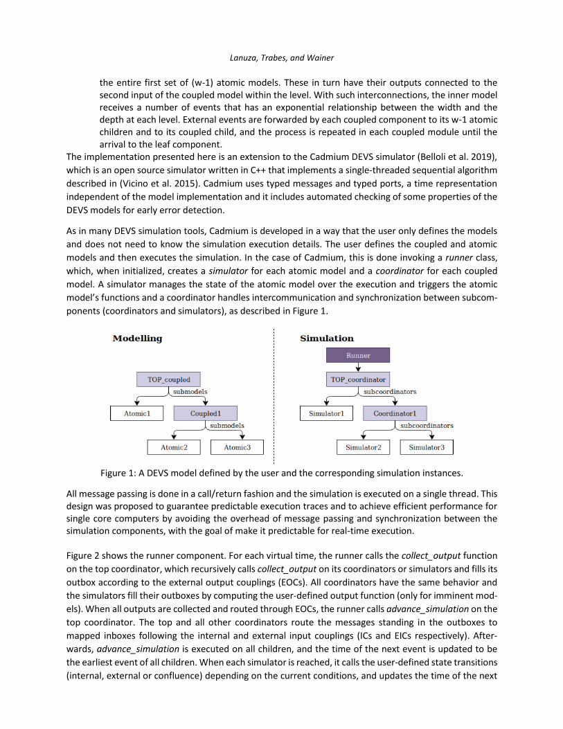
As in many DEVS simulation tools, Cadmium is developed in a way that the user only defines the models
and does not need to know the simulation execution details. The user defines the coupled and atomic
models and then executes the simulation. In the case of Cadmium, this is done invoking a runner class,
which, when initialized, creates a simulator for each atomic model and a coordinator for each coupled
model. A simulator manages the state of the atomic model over the execution and triggers the atomic
model’s functions and a coordinator handles intercommunication and synchronization between subcom-
ponents (coordinators and simulators), as described in Figure 1.
Figure 1: A DEVS model defined by the user and the corresponding simulation instances.
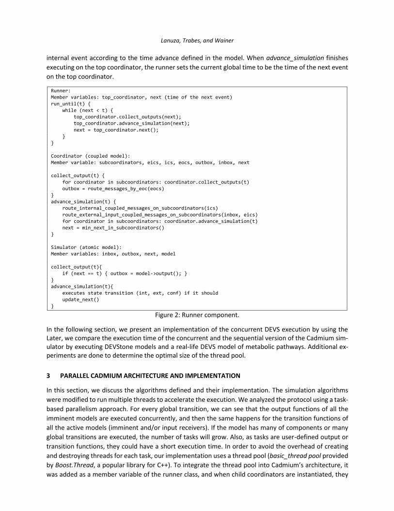
All message passing is done in a call/return fashion and the simulation is executed on a single thread. This design was proposed to guarantee predictable execution traces and to achieve efficient performance for single core computers by avoiding the overhead of message passing and synchronization between the simulation components, with the goal of make it predictable for real-time execution. Figure 2 shows the runner component. For each virtual time, the runner calls the collect_output function
on the top coordinator, which recursively calls collect_output on its coordinators or simulators and fills its
outbox according to the external output couplings (EOCs). All coordinators have the same behavior and
the simulators fill their outboxes by computing the user-defined output function (only for imminent mod-
els). When all outputs are collected and routed through EOCs, the runner calls advance_simulation on the
top coordinator. The top and all other coordinators route the messages standing in the outboxes to
mapped inboxes following the internal and external input couplings (ICs and EICs respectively). After-
wards, advance_simulation is executed on all children, and the time of the next event is updated to be
the earliest event of all children. When each simulator is reached, it calls the user-defined state transitions
(internal, external or confluence) depending on the current conditions, and updates the time of the next
Lanuza, Trabes, and Wainer
internal event according to the time advance defined in the model. When advance_simulation finishes
executing on the top coordinator, the runner sets the current global time to be the time of the next event
on the top coordinator.
Runner:
Member variables: top_coordinator, next (time of the next event)
run_until(t) {
while (next < t) {
top_coordinator.collect_outputs(next);
top_coordinator.advance_simulation(next);
next = top_coordinator.next();
}
}
Coordinator (coupled model):
Member variable: subcoordinators, eics, ics, eocs, outbox, inbox, next
collect_output(t) {
for coordinator in subcoordinators: coordinator.collect_outputs(t)
outbox = route_messages_by_eoc(eocs)
}
advance_simulation(t) {
route_internal_coupled_messages_on_subcoordinators(ics)
route_external_input_coupled_messages_on_subcoordinators(inbox, eics)
for coordinator in subcoordinators: coordinator.advance_simulation(t)
next = min_next_in_subcoordinators()
}
Simulator (atomic model):
Member variables: inbox, outbox, next, model
collect_output(t){
if (next == t) { outbox = model->output(); }
}
advance_simulation(t){
executes state transition (int, ext, conf) if it should
update_next()
}
Figure 2: Runner component.
In the following section, we present an implementation of the concurrent DEVS execution by using the Later, we compare the execution time of the concurrent and the sequential version of the Cadmium sim-ulator by executing DEVStone models and a real-life DEVS model of metabolic pathways. Additional ex-periments are done to determine the optimal size of the thread pool.
3 PARALLEL CADMIUM ARCHITECTURE AND IMPLEMENTATION
In this section, we discuss the algorithms defined and their implementation. The simulation algorithms
were modified to run multiple threads to accelerate the execution. We analyzed the protocol using a task-
based parallelism approach. For every global transition, we can see that the output functions of all the
imminent models are executed concurrently, and then the same happens for the transition functions of
all the active models (imminent and/or input receivers). If the model has many of components or many
global transitions are executed, the number of tasks will grow. Also, as tasks are user-defined output or
transition functions, they could have a short execution time. In order to avoid the overhead of creating
and destroying threads for each task, our implementation uses a thread pool (basic_thread pool provided
by Boost.Thread, a popular library for C++). To integrate the thread pool into Cadmium’s architecture, it
was added as a member variable of the runner class, and when child coordinators are instantiated, they

Lanuza, Trabes, and Wainer
save a reference to that thread pool. When the coordinators execute the collect_output and advance_sim-
ulation functions, they submit the recursive calls to the thread pool instead of executing it in the same
thread.
Coordinator (coupled model)
collect_output(t) {
concurrent_for_each(thread pool, subcoordinators.begin(), subcoordinators.end(), collect_outputs)
_outbox = route_messages_by_eoc()
}
advance_simulation(t) {
Route the messages standing in the outboxes to
mapped inboxes following ICs and EICs
concurrent_for_each(thread pool, subcoordinators.begin(), subcoordinators.end(), advance_simula-
tion)
_next = min_next_in_subcoordinators()
}
Figure 3: concurrent coordinator component.
On the Figure 3, we show the concurrent coordinator. A helper function concurrent_for_each was defined to abstract the concurrent execution. This function submits all tasks received by the parameter to the thread pool, and the function does not return until all the tasks are finished. The execution of all tasks is guaranteed because in the worst case scenario (when all threads in the pool are busy) the current thread will execute sequentially. Figure 4 shows concurrent_for_each. concurrent_for_each(basic_thread_pool thread pool, ITERATOR first, ITERATOR last, FUNC& f) {
vector<future<void>> task_statuses;
for (auto it= first; it != last; it++) {
packaged_task<void> task(bind(f, *it));
task_statuses.push_back(task.get_future());
thread pool.submit(task);
}
while(!all_of(task_statuses.begin(), task_statuses.end(), future_ready))) {
// if there are tasks wait to be executed, the current thread executes one
thread pool.schedule_one_or_yield();
}
// when concurrent_for_each ends, all tasks have been executed
}
Figure 4: concurrent_for_each function.
Regarding correctness, it is trivial to notice that all the outputs functions (called in collect_output) are executed before all transitions (called in advance_simulation). What is not clear is that all the output mes-sages are routed correctly through the couplings before calling the transition functions. For each coordi-nator in the coordinator tree, collect_output executes in all its children (if they are simulators, the outbox is filled with the result of the output function) and then the coordinator fills its outbox according to EOCs, leaving it full for the coordinator one level up. The advance_simulation function is not called until the outboxes on all levels are full. Afterwards, for each level, the messages are routed through EICs and ICs before calling to advance simulation on its children (which end up executing the transition functions). The next event time is set correctly because it is calculated after the coordinators finish advancing the simu-lation and updating their next event time.
4 EXPERIMENTAL RESULTS
In this section we present an empirical evaluation for the implementation proposed (which is available at
https://github.com/SimulationEverywhere/). Several experiments were made in order to compare the

Lanuza, Trabes, and Wainer
concurrent solution with the sequential algorithm. Experiments involve studying execution times of
DEVStone models to understand how different properties of the model impact the speedup of the parallel
algorithm. The execution time of both implementations was also measured with a real DEVS model of
metabolic pathways. Finally, speedup was studied in relation to the number of threads used in the execu-
tion. All the experiments were executed on a computer using an Intel i7 -7700 CPU with 4 cores and hy-
perthreading support for two threads per core. Unless specified otherwise, each experiment was executed
using 8 threads, the main thread and 7 for the threads pool. This value was used because it is the number
of threads specified by the hardware.
For the first experiment, we executed DEVStone models type LI and HI using a fixed value for depth (D=5)
and width (W=20), and a variable number of executions of the Dhrystone benchmark in the internal and
external transitions of each atomic model. In all the executions, the number of internal transitions is equal
to the number of the external transition.
Figure 5. LI model with Depth=5 and width=20 Figure 6. HI model with Depth=5 and width=20
Figure 5 shows the execution time of an LI model using the sequential and the concurrent implementa-
tions and the speedup obtained by the concurrent version. Figure 6 shows the results of the same exper-
iment for the HI model. In both models, when each transition function has a larger execution time, the
time of the concurrent algorithm is much smaller than the sequential one, getting up to a speedup of 2
(50% of execution time). For smaller execution time of the transitions, less speedup is achieved and even
in some cases, the sequential version ends up being faster than the concurrent. Also, the execution time
in both algorithms seem to grow linearly as a function of the number of operations executed and for both
models, the speedup gets up to a value around 2, and then remains constant.
Based on the results of this experiment, we decided to study more in detail models with transition func-
tions with a small number of computations. For this experiment, we simulated LI and HI models of differ-
ent sizes and we set internal and external transitions to execute only one Dhrystone benchmark operation
execution. Results are shown in Figure 7 for the LI topology and in Figure 8 for the HI.

Lanuza, Trabes, and Wainer
Figure 7. LI model. Figure 8. HI model.
The results suggest that if the model is big enough, even when only small computations are done in tran-
sition functions, the concurrent algorithm will outperform the sequential. This behavior for large models
could be explained by many tasks being sent to the thread pool queue in a short period of time. Conse-
quently, when a thread finishes one task, it directly continues with the next one, already in the queue,
and does not allow another process to run. For small models, the number of tasks that each thread exe-
cutes until they all must be synchronized is much smaller and could also lead to an unbalanced workload
between threads.
The next experiment is based on the predications from (Zeigler 2017) where is stated that the probability
of a model being imminent, and the effect of coupling are two important parameters that affect the
speedup of concurrent execution of the DEVS protocol. In the following experiment, we measure the
speedup of the four different types of DEVStones topologies (LI, HI, HO, HOmod) and measure their level
of activity and coupling. This was done using internal_cycles=2000, external_cycles=2000, D= 3 and W=40.
We used two empirical metrics to evaluate the level of activity and coupling of models:
level_of_activity = (#internal transitions + #confluence transitions) / (#atomics x #global transi-
tions)
level_of_coupling = (#external transitions + #confluence transitions) / (#atomics x #global transi-
tions)
The level_of_activity represents the estimated probability of a model having an internal transition at a
given instant and the level_of_coupling represents the probability of a model receiving an input (which
executes an external transition) at a given virtual time.
Table 1. DEVStones results summary
Sequential exe-
cution time (s)
Concurrent exe-
cution time (s)
Speedup
level_of_activity
level_of_coupling
LI 0.4870 0.2451 1.9868 0.923 0.911
HI 9.5841 5.252250 1.8247 0.923 0.948
HO 10.2476 5.8990 1.7372 0.923 0.948
HOmod 212.8980 108.8790 1.9553 0.544 0.580
On Table 1, a comparison between different DEVStone execution performance is presented. For all four
types of DEVStone models, the concurrent version’s execution time is considerably smaller than the se-
quential. On the other side, levels of activity and coupling for all of them have very high values and do not

Lanuza, Trabes, and Wainer
seem to represent accurately most real-life DEVS models.
To test our implementation on a real-world problem, we made another experiment where we compared
by execution times of both algorithms on a complex real DEVS model of metabolic pathways (Belloli et al.
2016). The model structure has 1608 atomic models and 23 coupled models distributed in 4 levels of
hierarchy. Additionally, both metrics of level_of_activity and level_of_coupling were calculated for the
model.
The results from executing this problem are the following ones:
Sequential execution time (in seconds): 90.8599
Concurrent execution time (in seconds): 51.4995
Speedup: 1.7643
level_of_activity: 0.2585
level_of_coupling: 0.2665
As it can be seen, even though the metrics of the level of activity and level of coupling are much lower
than for the different DEVStone topologies, there is still a considerable speedup in execution.
In the last experiment, we measured the execution times of simulating DEVStones and the metabolic
pathway models using different numbers of threads. DEVStone models of the four topologies were simu-
lated using width=100, depth=5, internal_cycles=200 and external_cycles=200.
Figure 9. Speedup of DEVS models with different number of threads.
Results are shown in Figure 9. The total number of threads from the x axis includes the main thread and
the threads from the thread pool. The DEVStone models seem to have a very similar behavior: if less than
5 threads are used the sequential algorithm is faster than the concurrent one (speedup is smaller than 1)
and for a larger number of threads the speedup grows until it reaches its peak with 8 or 9 threads. For
bigger values the speedup declines.
When the size of the thread pool is too small, the performance gains of using multiple threads declines
and the overhead of the communication between threads becomes an important factor. If the number of
threads used is too big, then scheduling overheads grow because of excessive context switching and
memory resources are wasted resulting in a performance decline. The best value is close to 8 threads,
which seems to be highly correlated with the number of simultaneous threads supported by the hard-
ware.

Lanuza, Trabes, and Wainer
Results for the metabolic pathway model also show an important increase in speedup from using 2
threads to 3, but after that the slope declines and no considerable improvements are obtained by using
more threads. This is related to the number of tasks submitted in each global transition and the internal
structure of the model.
5 CONCLUSIONS AND FUTURE WORK
In this work we presented an implementation for the DEVS protocol to execute in parallel in multithread-
ing architectures. We discussed the details in this implementation, and we show an empirical evaluation
with benchmarks models and a real application. The results obtained show how this implementation can
achieve lower execution times and therefore speedup over the sequential version. As future work we
propose to evaluate this implementation on different multithreading architectures and to implement ad-
ditional real applications to test the advantage of using this implementation.
REFERENCES
Adegoke A., H. Togo, and M.K. Traoré, “A Unifying Framework for Specifying DEVS Parallel and Distrib-
uted Simulation Architectures,” SIMULATION, vol. 89, no. 11, 2013, pp. 1293–1309.
Belloli, L. Vicino D., C. Ruiz-Martin and G. Wainer. 2019. “Building DEVS Models with the Cadmium Tool”.
In Proceedings of the 2019 Winter Simulation Conference, edited by N. Mustafee, K.-H.G. Bae, S.
Lazarova-Molnar, M. Rabe, C. Szabo, P. Haas, and Y.-J. Son, pp. 45–59. Piscataway, New Jersey, Insti-
tute of Electrical and Electronics Engineers, Inc.
Belloli, L., G. Wainer, and R. Najmanovich. 2016. "Parsing and Model Generation for Biological Pro-
cesses." in Proceedings of the Symposium on Theory of Modeling and Simulation (TMS-DEVS). IEEE.
(art. 21) Pasadena, CA, USA.
Cardoen, B., S. Manhaeve, Y. Van Tendeloo, Y., and J. Broeckhove. 2018. “A PDEVS simulator supporting
multiple synchronization protocols: implementation and performance analysis”. SIMULATION, 94(4),
281–300.
Chow, A. and B. P. Zeigler. 1994. “Parallel DEVS: a parallel, hierarchical, modular, modeling formalism”.
In Proceedings of the 1994 Winter Simulation Conference, edited by J. D. Tew, S. Manivannan, D. A.
Sadowski, and A. F. Seila, pp. 716–722. Piscataway, New Jersey, Institute of Electrical and Electronics
Engineers, Inc.
Chow, A.C., B. P. Zeigler and D. H. Kim. 1994. "Abstract Simulator for the Parallel DEVS Formalism". Proc.
of the Fifth Conference on AI, Simulation, and Planning in High Autonomy Systems, (pp. 157-163)
Gainesville, FL.
Dagum, L. and R. Menon. 1998. "OpenMP: an industry standard API for shared-memory programming."
Computational Science & Engineering IEEE, vol. 1, no. 5, pp. 46-55.
Hennessy J.L. and David A. Patterson. 2011. Computer Architecture, A Quantitative Approach (5th. ed.).
San Francisco, CA, USA: Morgan Kaufmann Publishers Inc.
Fujimoto R. M. 1999. Parallel and Distribution Simulation Systems (1st. ed.). New York, NY, USA: John
Wiley & Sons, Inc.
Fujimoto R. M. 1990. Parallel discrete event simulation, Communications of the ACM, 33(10), 30–53.

Lanuza, Trabes, and Wainer
Jafer, S. and G. Wainer. 2011. “Conservative synchronization methods for parallel DEVS and Cell-DEVS”.
In Proceedings of the 2011 Summer Computer Simulation Conference (SCSC ’11). pp. 60-67. Vista, CA:
Society for Modeling & Simulation International.
Jafer S., Q. Liu, G. Wainer. 2013. “Synchronization methods in parallel and distributed discrete-event sim-
ulation”, Simulation Modelling Practice and Theory, Volume 30, Pages 54-73.
Liu, Q. and G. Wainer. 2009. "A Performance Evaluation of the Lightweight Time Warp Protocol in Opti-
mistic Parallel Simulation of DEVS-Based Environmental Models," ACM/IEEE/SCS 23rd Workshop on
Principles of Advanced and Distributed Simulation, Lake Placid, NY, pp. 27-34
Nutaro, J. “On Constructing Optimistic Simulation Algorithms for the Discrete Event System Specification”.
ACM Transactions on Modeling and Computer Simulation (TOMACS). Vol. 19, No. 1. January 2019.
Nyman L. and M. Laakso. 2016. "Notes on the History of Fork and Join," in IEEE Annals of the History of
Computing, vol. 38, no. 3, pp. 84-87.
Schmidt D. C. and S. Vinoski. 1996. “Object Interconnections: Comparing Alternative Programming
Techniques for Multithreaded Servers the Thread-Pool Concurrency Model”, C++ Report, SIGS, Vol 8,
No 4.
Vicino D., D. Niyonkuru, G. Wainer, and O. Dalle. 2015. “Sequential PDEVS architecture”. In Proceedings
of the Symposium on Theory of Modeling & Simulation: DEVS Integrative M&S Symposium (DEVS
’15), edited by. Society for Computer Simulation International, San Diego, CA, USA, 165–172.
Wainer, G., E. Glinsky and M. Gutierrez-Alcaraz, 2011 "Studying Performance of DEVS Modeling and Sim-
ulation Environments using the DEVStone Benchmark," Simulation, vol. 87, no. 7, pp. 555-580.
Weicker, R. P. 1984. “Dhrystone: a synthetic systems programming benchmark”. Commun. ACM vol. 27,
no. 10, pp. 1013-1030.
Zeigler, B.P., H. Praehofer and T. G. Kim. 2000. Theory of modeling and simulation: Integrating Discrete
Event and Continuous Complex Dynamic Systems, San Diego, CA: Academic Press.
Zeigler, B. 2017. "Using the Parallel DEVS Protocol for General Robust Simulation with Near Optimal Per-
formance". Computing in Science & Engineering, vol. 19, no. 03, pp. 68-77.
AUTHOR BIOGRAPHIES
JUAN LANUZA is a Licenciate degree student in Computer Science at the Department of Computer Science
at University of Buenos Aires. His email is [email protected].
GUILLERMO G. TRABES is a Ph.D. student in Electrical and Computer Engineering (Carleton University)
and Computer Science (Universidad Nacional de San Luis). His email address is [email protected]
leton.ca.
GABRIEL A. WAINER is Professor at the Department of Systems and Computer Engineering at Carleton
University. He is a Fellow of the Society for Modeling and Simulation International (SCS). His email address
Related Documents


