Parallel Algorithms for Adding a Collection of Sparse Matrices

Parallel Algorithms forAdding a Collection of Sparse Matrices

Md Taufique Hussain∗, Guttu Sai Abhishek† Aydin Buluc‡ and Ariful Azad§∗ Indiana University, Bloomington, IN, USA ([email protected])

† IIT Bombay, India ([email protected])‡ Lawrence Berkeley National Laboratory, Berkeley, CA, USA ([email protected])

§ Indiana University, Bloomington, IN, USA ([email protected])

Abstract—We develop a family of parallel algorithms for theSpKAdd operation that adds a collection of k sparse matrices.SpKAdd is a much needed operation in many applications in-cluding distributed memory sparse matrix-matrix multiplication(SpGEMM), streaming accumulations of graphs, and algorithmicsparsification of the gradient updates in deep learning. Whileadding two sparse matrices is a common operation in Matlab,Python, Intel MKL, and various GraphBLAS libraries, theseimplementations do not perform well when adding a large col-lection of sparse matrices. We develop a series of algorithms usingtree merging, heap, sparse accumulator, hash table, and slidinghash table data structures. Among them, hash-based algorithmsattain the theoretical lower bounds both on the computationaland I/O complexities and perform the best in practice. The newly-developed hash SpKAdd makes the computation of a distributed-memory SpGEMM algorithm at least 2x faster than that theprevious state-of-the-art algorithms.

I. INTRODUCTION

Sparse matrices power many modern scientific codes, in-cluding those that arise in simulations, data analytics, andmachine learning. An overlooked operation that is commonacross many applications is the summation (or reduction) of acollection of sparse matrices. In the deep learning community,this is called the sparse allreduce problem [1], [2] thatarises due to algorithmic sparsification of the gradient updatesfor reduced communication. While most papers describe theproblem as the reduction of sparse vectors, each holdinggradient updates from one processor, in practice the computa-tion becomes the reduction of a collection of sparse matricesdue to mini-batching commonly used in gradient-based deeplearning training. The existing work on this sparse allreduceproblem is exclusively on the communication and distributed-memory aspects, leaving the actual in-node reduction itselfunderstudied.

The use case that primarily motivated our work is thedistributed-memory multiplication of two sparse matrices(SpGEMM). In virtually all algorithms for the distributedmemory SpGEMM, there is a step where each processor hasto sum intermediate products of the form

∑ki=1 AiBi. We

call this operation SpKAdd. While local SpGEMM algorithmshave seen significant advances in their performance within thelast 15 years [3], SpKAdd has not received any attention, leav-ing it a potential bottleneck. This is especially true when we tryto achieve strong scaling or when there is overdecompositionof the problem for ease of load balancing: the more processes

perform distributed SpGEMM, the more computation shiftsfrom local SpGEMMs to SpKAdd. This seemingly counter-intuitive fact is easy to verify when considering the extremecase where each process owns a single 1×1 matrix and thereare n2 processors for multiplying two n×n sparse matrices:SpKAdd does half the flops (i.e., all the additions) neededfor the distributed SpGEMM. Furthermore, communication-avoiding SpGEMM algorithms [4], [5] utilize SpKAdd at twodifferent phases: one within each 2D grid of the overall 3Dprocess grid and another when reducing results across different2D grids.

Finally, SpKAdd is needed for assembling local finite-element matrices into a global matrix [6]. This problem hastraditionally been labeled as one that presents few opportu-nities for parallelism. In this work, we show this not to betrue. In fact, SpKAdd has plenty of parallelism. However,existing implementations use suboptimal data structures forthe accumulation, hurting their performance. In this paper, wesystematically evaluate various different data structures andmethods for SpKAdd in shared memory.

The main contribution of this paper is to develop efficientparallel SpKAdd algorithms that are work-efficient, use spatiallocality when accessing memory, and do not require threadsynchronization. We achieve these goals by utilizing heap,sparse accumulator (SPA) [7], hash table data structures. Wedesigned a sliding hash algorithm after carefully considering(a) the data access patterns for different data structures, (b)matrix shapes and sparsity patterns, and (c) hardware featuressuch as the cache size. We theoretically and experimentallydemonstrate that hash and sliding hash based SpKAdd algo-rithms run the fastest for input matrices with various shapesand sparsity patterns on three different shared-memory plat-forms. We demonstrate the impact of fast SpKAdd algorithmsby plugging the hash algorithm in a distributed SpGEMMimplementation in the CombBLAS library [8]. When runningSpGEMM on 2K nodes of a Cray XC40 supercomputer, thehash-based SpKAdd made the computation of the distributedSpGEMM 2× faster than the previous implementation.

arX

iv:2

112.

1022

3v1

[cs

.DC

] 1

9 D

ec 2

021

Algorithm 1 SpKAdd using 2-way addition of columns.Input: A list of k sparse matrices A1, ...,Ak. Output: B. Allmatrices are in Rm×n

1: procedure SPKADD2WAY(A1, ...,Ak)2: B← A1

3: for i← 2 to k do4: for j ← 1 to n do5: B(:, j)← ColAdd (B(:, j),Ai(:, j))6: return B

II. ALGORITHMIC LANDSCAPE OF THESPKADD OPERATION

A. The problem

We consider the operation SpKAdd that adds k sparsematrices A1,A2, ...,Ak and returns the summed (poten-tially sparse) matrix B=

∑ki=1 Ai, where Ai∈Rm×n and

B∈Rm×n. We assume that all input matrices A1,A2, ...,Ak

are available in memory before performing the SpKAddoperation. Let nnz(Ai) denote the number of nonzeros in Ai.Then, nnz(B) ≤∑k

i=1 nnz(Ai). The compression factor cf ofan SpKAdd operation is defined as

∑ki=1 nnz(Ai)/nnz(B),

where cf ≥1. When k=2, the operation simply adds two sparsematrices. In this special case of k=2, SpKAdd is equivalent tomkl_sparse_d_add in MKL, the “+” operator in Matlaband Python (with scipy sparse matrices as operands). Whileadding two sparse matrices sequentially or in parallel is awidely-implemented operation in any sparse matrix library,SpKAdd is rarely implemented in most libraries. One canrepeatedly add sparse matrices in pairs to add k sparsematrices. However, we will analytically and experimentallydemonstrate that the pairwise addition could be significantlyslower than a unified SpKAdd operation when k is large.

Throughout the paper, we assume that input and outputmatrices are represented in the compressed sparse column(CSC) format that stores nonzero entries column by column.However, all algorithms discussed in this paper are equally ap-plicable to compressed sparse row (CSR), coordinate (COO),doubly compressed, and other sparse matrix formats [9].

B. SpKAdd using 2-way additionsAt first, we describe SpKAdd algorithms that rely on 2-way

addition of a pair of matrices. We have implemented parallel2-way additions in our library, but an implementation fromMKL, Matlab, and GraphBLAS [10], [11] can be used.

1) SpKAdd using 2-way incremental additions: The sim-plest approach to implement SpKAdd is to incrementally addk sparse matrices in pairs. Algorithm 1 provides a skeletonof SpKAdd implemented with 2-way incremental additions.Here, the ith iteration of the outer loop adds the current partialresult with the next input matrix Ai. Since matrices are storedin the CSC format, the jth columns of Ai and B can be addedindependently as denoted by the ColAdd operation in line 5of Algorithm 1. Here, the jth columns of a matrix is an array of(rowid, val) tuples where rowid denotes the row indexof a nonzero entry. If columns are sorted in the ascending

order of row index, the ColAdd function simply merges twolists of tuples, which is similar to the merging operation ofthe merge sort algorithm. Fig. 1(b) shows an example of 2-way incremental addition for the jth columns of four matricesshown in Fig. 1(a).

Computational complexity. First, consider the cost ofadding two matrices A1 and A2. If each columns are sortedbased on their row indices, a linear merging algorithm hasO(nnz(A1)+nnz(A2)) complexity. Even though faster merg-ing algorithm exists for imbalanced lists [12], they often aretoo complicated for parallel implementations. In the worst casewhere the matrices have no common row indices, nnz(A1 +A2) = nnz(A1) + nnz(A2). This is especially true whennonzeros in the input matrices are uniformly distributed suchas in Erdos-Renyi (ER) random matrices. In this worst-casemodel, the ith iteration of the 2-way incremental algorithm hasthe cost of

∑il=1 nnz(Al) and the total cost of the algorithm

is∑k

i=2

∑il=1 nnz(Al). If all input are ER matrices with

d nonzeros per column, the overall computational cost is∑ki=2

∑il=1 nd = O(k2nd).

I/O complexity. In this paper, the I/O complexity measuresthe amount of data transferred to and from the main memory. Ifwe assume that the output of every 2-way addition is stored inthe main memory, the I/O complexity of the 2-way incrementalalgorithm matches the computational complexity discussedabove. That means O(k2nd) data is accessed from the mainmemory for ER matrices.

2) SpKAdd using 2-way tree additions: The 2-way incre-mental addition is expensive both in terms of the computa-tional complexity and data movements. One reason of thisinefficiency is the imbalanced nature of the binary additiontree shown in Fig. 1(b) where the height of the tree isk − 1. To address this problem, we consider a balancedbinary tree as shown in Fig. 1(c) where the height of thetree is lg k. In the 2-way tree addition, input matrices areadded in pairs in the leaves of the tree before the resultantmatrices are added at internal nodes. Thus, the computationalcomplexity of all additions at a given level of the binary tree isO(

∑ki=1 nnz(Ai)), which results in the overall complexity of

O(lg k∑k

i=1 nnz(Ai)). Assuming that the intermediate matri-ces are stored in memory, the amount of data movement is alsoO(lg k

∑ki=1 nnz(Ai)). For ER input matrices, the computa-

tional and data movement complexity become O(ndk lg k).Hence, for any large value of k, 2-way tree addition is fasterthan 2-way incremental addition both in theory and in practice.This performance improvement comes for free as we can stilluse any off-the-shelf function to add a pair of matrices.C. SpKAdd using k-way additions

Since repeated use of 2-way additions leads to an inefficientSpKAdd operation, we developed several algorithms that usek-way additions. Algorithm 2 provides a template for such analgorithm where jth columns of all input matrices are addedto form the jth column of the output. Line 3 of Algorithm 2calls the k-way addition of columns for which we consideredseveral data structures including heaps, sparse accumulators,and hash tables.

(1,3)(3,2)(6,1)

(0,2)(3,1)(5,3)

(5,2)(7,1)

(1,2)(6,1)(7,3)

(0,2)(1,5)(3,3)(5,5)(6,2)(7,4)

+ + + =

(1,3)(3,2)(6,1)

+ (0,2)(3,1)(5,3)

(0,2)(1,3)(3,3)(5,3)(6,1)

(5,2)(7,1)

(1,2)(6,1)(7,3)

+

(1,3)(3,2)(6,1)

+

(0,2)(3,1)(5,3)

(0,2)(1,3)(3,3)(5,3)(6,1)

+

(1,2)(5,2)(6,1)(7,4)

(5,2)(7,1)

(1,2)(6,1)(7,3)

+

(0,2)

(1,5)

(3,3)

(5,5)

(6,2)

(7,4)

+

(0,2)

(1,3)

(3,3)

(5,5)

(6,1)

(7,1)

(0,2)(1,5)(3,3)(5,5)(6,2)(7,4)

(1,1,3)

(0,2,2)

(5,3,2)

(1,4,2) (1,4,2)

(1,1,3)

(5,3,2)

(3,2,1) (3,1,2)

(1,4,2)

(5,3,2)

(3,2,1)

(0,2) (0,2)(1,3)

(0,2)(1,5)

heap

current output

heap heap

(1,3)(3,2)(6,1)

(1,3)(3,2)

(6,1)

(0,2)(1,3)(3,3)(5,3)(6,1)

table(0,2)(1,3)(3,3)(5,5)(6,1)(7,1)

tableA1(:,j)(0,2)(3,1)(5,3)

(5,2)(7,1)

After col 1 After col 2 After col 3

(0,2)(1,3)

(3,3)

(5,5)(6,1)(7,1)

(1,3)

(3,2)

(6,1)

(0,2)(1,3)

(3,3)

(5,3)(6,1)

(f) Hash table size: nnz(B(:,j)); op cost: O(1)#hash operations: ∑ 𝑛𝑛𝑧(𝐴!(: , 𝑗))"

!#$ ;

(d) Heap size: k; each op cost: O(lg k)#heap operations: ∑ 𝑛𝑛𝑧(𝐴!(: , 𝑗))"

!#$ ;

A2(:,j) A3(:,j)table

(e) SPA size: m; op cost: O(1)#SPA operations: ∑ 𝑛𝑛𝑧(𝐴!(: , 𝑗))"

!#$ ;

(1,3)(3,2)(6,1)

SPA SPAA1(:,j)(0,2)(3,1)(5,3)

(5,2)(7,1)

After col 1 After col 2 After col 3

A2(:,j) A3(:,j)SPA

A1(:,j) A2(:,j) A3(:,j) A4(:,j) B(:,j)

A1(:,j) A3(:,j) A4(:,j)A2(:,j)

B(:,j)

A1(:,j)A3(:,j) A4(:,j)A2(:,j)

B(:,j)

(b) 2-way Incremental: #2-way merge: k-1 Total ops: k* ∑ 𝑛𝑛𝑧(𝐴!(: , 𝑗))"

!#%

(c) 2-way tree: #2-way merge: k-1 Total ops: lgk ∗ ∑ 𝑛𝑛𝑧(𝐴!(: , 𝑗))"

!#%

(a) The SpKAdd operation for column j

HeapOperation 1

current output

current output

HeapOperation 2

HeapOperation 3

Fig. 1: Data structure and algorithmic choices when adding the jth columns of four input matrices. (a) Input and outputcolumns, where each column stores (rowid, value) tuples. Different colors are used to show different input columns. (b) 2-wayincremental addition. (c) 2-way tree addition where inputs are at the leaves of a binary tree. (d) k-way addition using a min-heap of size k = 4. The heap stores (rowid, matrixid, value) tuples and holds at most one entry from each input column. Theentry with the minimum row index is at the root of the tree representing the min-heap. Only the first three heap operations(extracting the minimum entry and inserting another entry) are shown. We also show the current status of the output column.(e) k-way addition using a SPA of size m = 8. Any entry from the ith row of an input matrix such as A1(i, j) is added to theith entry of the SPA. (f) k-way addition using a hash table of size B(:, j) = 6. For simplicity of depiction, we assume that thehash function maps row indices to hash table in the ascending order of row indices in B(:, j) (e.g., B(5, j)) is the 4th entryof the output and mapped to the 4th position of the hash table).

Algorithm 2 SpKAdd using k-way addition of columns.Input: A list of k sparse matrices A1, ...,Ak; Output: B. Allmatrices are in Rm×n

1: procedure SPKADD(A1, ...,Ak)2: for j ← 1 to n do3: B(:, j)← ColAddKWay (A1(:, j), ...,Ak(:, j)) .

HeapAdd, SPAAdd, HashAdd, etc.4: return B

1) HeapSpKAdd: k-way additions using a heap: Algo-rithm 3 shows the HeapAdd operation that uses a min-heap toadd jth columns of all input matrices. Here, Heap represents abinary tree storing k tuples with each (r, i, v) tuple representsv = Ai(r, j), i.e., v is stored in the rth row and jth columnof Ai. Each tuple in the heap has a unique matrix index (themiddle entry of the tuple), meaning that at most one tuplein the heap is from an input matrix. The min-heap uses rowindices as the key and stores the tuple with the minimum rowindex at the root. Hence, extracting a tuple with the minimumrow index takes O(1) time, but inserting a new entry to the

heap takes O(lg k) time. See Fig. 1(d) for an example.Lines 3-5 of Algorithm 3 initialize the heap with the

smallest row indices from all input columns. Each iteration ofthe loop at line 6 extracts the minimum entry (r, i, v) (basedonly on the row index) from the heap. If this is the first timewe extract an entry from row r, we append (r, v) at the the endof the output. If there is already an entry in the output columnat row r, we simply add v to this row index. Since the outputcolumn is formed in the ascending order of row indices, theexistence of B(r, j) in line 8 can be checked in O(1) time. Ifthe minimum entry from the heap came from Ai, we insertthe next entry from Ai into the heap (line 12-14). Here, theheap algorithm assumes that all columns of input matrices aresorted in the ascending order of row indices.

Complexity: Inserting a tuple to the heap takes O(lg k)time. Since every nonzero entry from the input must be in-serted to the heap for processing, the total computational com-plexity of the heap based algorithm is O(lg k

∑ki=1 nnz(Ai)),

which is equivalent to the 2-way tree algorithm algorithm. ForI/O complexity, we assume that the heap (of size O(k)) fits in a

Algorithm 3 SpKAdd using a min-heap. Only the addition ofjth columns is shown. The jth column A(:, j) is stored as alist of tuples (r, v) where r and v denote row index and value.

1: procedure HEAPADD(A1(:, j), ...,Ak(:, j))2: Heap ← φ3: for i← 1 to k do4: (r, v) ← the nonzero entry with the smallest row

index in Ai(:, j)5: INSERT(Heap, (r, i, v))6: while Heap 6= φ do7: (r, i, v)← EXTRACTMIN(Heap)8: if B(r, j) exists then9: B(r, j)← B(r, j) + v

10: else . append at the end of the output11: B(:, j)← B(:, j) ∪ (r, v)

12: if Ai still has unused entries then13: (rnext, vnext)← the next element from Ai

14: INSERT(Heap, (rnext, i, vnext))15: return B(:, j)

Algorithm 4 SpKAdd using a SPA. Only the addition of jthcolumns is shown. The jth column A(:, j) is stored as a listof tuples (r, v) where r and v denote row index and value.

1: procedure SPAADD(A1(:, j), ...,Ak(:, j))2: SPA← a dense array of length m3: idx ← φ . a list of valid indices in SPA4: for i← 1 to k do5: for (r, v) ∈ Ai(:, j) do6: if r ∈ idx then SPA[r]← SPA[r] + v7: else SPA[r]← v; idx ← idx ∪r8: SORT(idx ) . if sorted output is desired9: for r ∈ idx do

10: append (r,SPA[r]) into B(:, j)

11: return B(:, j)

thread-private cache and HeapSpKAdd streams input columnsfrom memory and writes the output column to memory withoutstoring any intermediate matrices. Thus, the I/O cost of theheap algorithm is O(

∑ki=1 nnz(Ai)). For ER matrices, the

computational and I/O complexity of HeapSpKAdd becomeO(ndk lg k) and O(ndk), respectively.

2) SPASpKAdd: k-way addition using a SPA: Algorithm 4describes the addition of columns using a SPA. We representSPA with two dense arrays SPA of length m (number of rowsin matrices) and idx of length nnz(B(:, j)). The rth entry ofSPA stores the value at the rth row of the output nnz(B(r, j)).The idx array stores the indices of SPA with valid entries.Each iteration of the loop at line 4 in Algorithm 4 processesthe input column from the i matrix. Consider an entry (r, v)from the current column Ai(:, j). If this row exists in the (idx)array (i.e., a valid entry exists at SPA[r ]), the value v is addedto the corresponding location at SPA (line 6). Otherwise, therow index r is inserted into the idx array. If sorted output isdesired the idx array is sorted before generating the result.

Algorithm 5 SpKAdd using a hash table. Only the addition ofjth columns is shown. The jth column A(:, j) is stored as alist of tuples (r, v) where r and v denote row index and value.

1: procedure HASHADD(A1(:, j), ...,Ak(:, j))2: HT ← an array whose size is a power of two and

greater than nnz(B(:, j)); initialized with (−1, 0)3: for i← 1 to k do4: for (r, v) ∈ Ai(:, j) do5: h← HASH(r) . hash index from row index6: while true do7: if HT [h] is empty then8: HT [h]← (r, v); break9: else if r is found at HT [h] then

10: add v to the value at HT [h]; break11: else . hash conflict resolution12: h← next hash index13: for every valid hash index h ∈ HT do14: append HT [h] into B(:, j)

15: SORT(B(:, j)) . if sorted output is desired16: return B(:, j)

See Fig. 1(e) for an example.Complexity. Since every nonzero entry from the input is

inserted once to SPA, the computational complexity of the SPAbased algorithm is O(

∑ki=1 nnz(Ai)). The I/O complexity is

also O(∑k

i=1 nnz(Ai)).3) HashSpKAdd: using k-way additions using a hash table:

Algorithm 5 shows the HashAdd operation that uses a hashtable HT to add jth columns of all input matrices. The size ofHT is a power of two and it is greater than nnz(B(:, j)) (whichis obtained via a symbolic phase discussed in Section II-D).The hash table HT stores r, v tuples of row indices and valuesfor all unique row indices in input columns. HT is initializedwith (−1, 0) where a negative row index denotes an unusedentry in the hash table.

Each iteration of the loop at line 3 in Algorithm 5 processesthe input column from the i matrix. Consider an entry (r, v)from the current column Ai(:, j). A suitable hash function isused to map the row index r to a hash index h (line 5). Inour implementation, we used a multiplicative masking schemeHASH(r) = (a ∗ r)&(2q − 1), where r is the row index usedas the hash key, a is a prime number, 2q is the size of thehash table with 2q ≥ nnz(B(:, j)). The bitwise and operator(&) masks off the bottom q bits so that the output of the hashfunction can be used as an index into a table of size 2q . Thewhile loop at line 6 search for the row index r in HT . If suchan entry is found, its value is updated in line 8. If not found(meaning that we encounter r for the first time), the currenttuple (r, v) is stored in HT (line 7). When a valid entry witha different row index is encountered (line 11), it indicates acollision in hash tables. We used the linear probing schemeto resolve collisions. After we process all input columns, weinsert all valid entries from the hash table to form the output.See Fig. 1(f) for an example.

Complexity. Inserting a value into a Hash table takes, on

Algorithm 6 Computing nnz(B(:, j)) using a hash table.

1: procedure HASHSYMBOLIC(A1(:, j), ...,Ak(:, j))2: HT ← an array whose size is a power of two and

greater than∑k

i=1 nnz(Ai); initialized with −13: nz ← 04: for i← 1 to k do5: for (r, v) ∈ Ai(:, j) do6: h← HASH(r) . hash index from row index7: while true do8: if HT [h] is empty then9: nz ← nz + 1

10: HT [h]← r; break11: else if r is found at HT [h] then break12: else h← next hash index13: return nz

the average case, O(1) time. Since every nonzero entry fromthe input is inserted to the hash table for processing, theaverage computational complexity of the hash based algorithmis O(

∑ki=1 nnz(Ai)). The I/O cost of the hash algorithm is

O(∑k

i=1 nnz(Ai)). For ER matrices, both the computationaland I/O complexity of HashSpKAdd become O(ndk).

D. The symbolic step to compute the output size

All k-way SpKAdd algorithms need to know nnz(B(:, j))for every column of the output to pre-allocate necessarymemory for the output. This estimation is also needed todetermine the hash table size. We pre-compute nnz(B(:, j))using a symbolic phase as shown in Algorithm 6. Here we usehash based symbolic phase, but heap and SPA could also beused to compute nnz(B(:, j)). The hash table in the symbolicphase needs to store indices only. Algorithm 6 first createsa hash table of size

∑ki=1 nnz(Ai) and initializes it with -1.

Then, similar to the actual addition (Algorithm 5), we searchfor the current row index r in the hash table. The first timer is found in the table, we increment the nonzero counterby one (lines 8-9). The computation and I/O complexity ofAlgorithm 6 is similar to that of Algorithm 5.

III. PARALLEL AND CACHE EFFICIENTSPKADD ALGORITHMS

A. Parallel algorithms

The way we design 2-way and k-way SpKAdd algorithmsmakes it very easy to parallelize them. Since each column ofB can be computed independently, we can parallelize line 4of Algorithm 1 and line 2 of Algorithm 2. This parallelizationstrategy does not require any thread synchronization and itdoes not depend on the data structure (heap, hash, SPA, etc.)used to add the jth columns of input matrices. In this case,we always execute Algorithms 3, 4 , 5, and 6 sequentially bya single thread. Note that parallelizing SpKAdd as a singlemultiway merging problem (e.g., when each matrix is stored asa list of (rowidx, colidx, val) tuples in the coordinate format) isnot a trivial task as it requires the lists to be partitioned amongthreads [13]. Even though SpKAdd (when dividing columnsamong threads) is an embarrassingly parallel problem, the

Algorithm 7 Computing nnz(B(:, j)) using a sliding hashtable. T : number of threads; M : total last-level cache; m:number of rows in matrices; b: number bytes needed for eachentry in the hash table (4 bytes for the symbolic phase).

1: procedure SLHASHSYMBOLIC(A1(:, j), ...,Ak(:, j))2: inz ←∑k

i=1 nnz(Ai)3: parts ← d(inz ∗b ∗ T )/Me4: nz ← 05: if parts=1 then . normal hash6: HASHSYMBOLIC(A1(:, j), ...,Ak(:, j))7: else . sliding hash8: for i← 1 to parts do9: r1 ← i ∗m/ parts; r2 ← (i+ 1) ∗m/ parts

10: nz ←nz + HASHSYMBOLIC(A1(r1 :r2, j), ...,Ak(r1 : r2, j))

11: return nz

choices of data structures, matrix shapes and sparsity patterns,and the memory subsystem of the computing platform playsignificant roles on the attained performance of SpKAdd .

The impact of data structures on the parallel perfor-mance. Our parallel SpKAdd algorithms maintain thread-private data structures (because Algorithms 3, 4 , 5, and 6 areexecuted sequentially). Hence the total memory requirementsfor different data structures across T threads are as follows:heap: O(T ·k), SPA: O(T ·m), Hash: O(T ·maxni=1 nnz(Bi)).The higher memory requirement of SPA may make the corre-sponding algorithm very slow because the algorithm accessesSPA at random locations. For example, if matrices have 32Mrows, and 48 threads are used, the memory requirement forSPA could be more than 100GB. In contrast the memory re-quirement of heap is very small. However, the heap algorithmaccesses all matrices concurrently (see Figure 1(d)). This couldcreate bandwidth bottleneck if different matrices are stored inmultiple sockets of a shared-memory platform.

Impact of matrix shapes and sparsity patterns onload imbalance. The computations in different columns ofSpKAdd are fairly load balanced when nonzeros in input ma-trices are uniformly distributed such as in Erdos-Renyi matri-ces. However, for matrices with skewed nonzero distributionssuch as RMAT matrices, the computations can vary dramati-cally across columns. In the latter case, a static scheduling ofthreads hurts the parallel performance of the algorithm. In thesymbolic phase we use total input non-zeros per column andin addition phase we use total output non-zeros per column tobalance loads dynamically.

B. The Sliding Hash algorithm

In Algorithm 6 and Algorithm 5 we used a single hash tablefor the computation of the entire column of the output. Theseapproaches work perfectly well as long as all hash tables usedby all threads fit in the last level cache. To understand thememory requirements of hash tables, let M be the size of lastlevel cache in bytes, T be the number of threads and b be thenumber of bytes needed to store each entry in the hash table.When 32 bit indices and single-precision floating point values

Algorithm 8 SpKAdd using a sliding hash table. T : numberof threads; M : total last-level cache; m: number of rows inmatrices; b: number bytes needed for each entry in the hashtable (8 bytes for 32 bit indices and values).

1: procedure SLHASHADD(A1(:, j), ...,Ak(:, j))2: onz ← SLHASHSYMBOLIC(A1(:, j), ...,Ak(:, j))3: parts ← d(onz ∗b ∗ T )/Me4: nz ← 05: if parts=1 then . normal hash6: HASHADD(A1(:, j), ...,Ak(:, j))7: else . sliding hash8: for i← 1 to parts do9: r1 ← i ∗m/ parts ; r2 ← (i+ 1) ∗m/ parts

10: B(r1:r2, j)← HASHADD(A1(r1 :r2, j), ...,Ak(r1 : r2, j))

11: return B(:, j)

are stored, b is 4 bytes for the symbolic phase and 8 bytes forthe addition phase. Then, the total hash table memory requiredfor the symbolic phase is MemSym = b∗T∗∑k

i=1 nnz(Ai(:, j))bytes. Similarly, the total hash table memory required foraddition phase is MemAdd= b∗T ∗nnz(B(:, j)) bytes. If eitherMemSym or MemAdd is greater than M , the hash table goesout of cache. Since hash tables are accessed randomly, out ofcache accesses are quite expensive.

To address this problem, we designed a modified hashalgorithm that limit the size of hash tables so that they fitwithin the last level cache. For example, when MemAdd isgreater than M , we create each hash table with no more thanM/(b ∗ T ) entries so that all hash tables across threads fitin M bytes. Since such a collection of hash tables cannotcover the entire output column, we slide a hash table alongthe column to produce outputs. Hence, we call it the slidinghash algorithm.

Algorithm 7 and Algorithm 8 describes the symbolic andSpKAdd algorithms using sliding hash tables. In Algorithm 7we divide the required memory by M to determine the numberof parts (line 3). If the number of parts is one (i.e., all hashtables fit in M byes), we simply call Algorithm 6 (lines 5-6). Ifmore parts are needed, we partition rows equally (using binarysearches) and then call Algorithm 6 for each part (lines 8-11).Similarly, Algorithm 7 identifies the memory requirement forall hash tables and uses the sliding hash strategy (lines 8-11)when needed. Thus, the sliding hash algorithms ensure thathash tables accesses are always performed within the cache,which gives significant performance boosts when the numberof input matrices is large or when input matrices are denser.Note that hash tables in the symbolic phase could be largerthan hash tables in the addition phase. For example, whencf of an SpKAdd operation is 10, the symbolic phase maydemand 10× more memory for hash tables. Hence, the slidinghash table is more beneficial for the symbolic phase.

C. Summary of all SpKAdd algorithmsTable I shows the complexity summary of algorithms when

adding k ER matrices each with d nonzeros per column on

average. We observe that 2-way and heap algorithms are notwork efficient, and 2-way algorithms access more data frommemory than other algorithms. Thus, we expect 2-way andheap algorithms to run slower than other algorithms. Ourexperimental results confirm this theoretical prediction. Thememory requirements for various data structures also varysignificantly. SPA requires the most memory, while the heapalgorithm needs the least memory (assuming that k � m).The sliding hash algorithm allocates hash tables based on theavailable cache. Both SPA and hash algorithms accesses theirdata structures randomly. Random accesses can be a potentialperformance bottleneck if hash tables and SPA do not fitin the cache. The sliding hash table mitigates this problemby limiting the size of hash table. Finally, SPA and hashalgorithms can operate with unsorted input columns, but 2-way and heap algorithms require sorted inputs.

IV. RESULTS

A. Experimental setupExperimental platforms. Most of our experiments are

conducted on two different servers with Intel and AMDprocessors as described in Table II. To demonstrate the im-pact of our SpKAdd algorithms on a distributed SpGEMMalgorithm, we ran some experiments on the KNL partitionof Cori supercomputer at NERSC. We have implementedour in C/C++ programming language with OpenMP multi-threading. For distributed memory experiments, we pluggedin our code in the sparse SUMMA algorithm available in theCombinatorial BLAS (CombBLAS) library [8].

Datasets. We use two types of matrices for the evaluation.We generate synthetic matrices using matrix generator, andalso use publicly available protein similarity matrices. We useR-MAT [14], the recursive matrix generator, to generate twodifferent non-zero patterns of synthetic matrices representedas ER and RMAT. ER matrix represents Erdos-Renyi randomgraphs, and RMAT represents graphs with power-law degreedistributions used for Graph500 benchmark. These matricesare generated with R-MAT seed parameters; a=b=c=d=0.25for ER matrix and a=0.57, b=c=0.19, d=0.05 for G500 ma-trix. Most of our experiments use rectangular matrices withmore rows than columns (m > n). To generate k RMATmatrices for SpKAdd experiments, we create a matrix m×nmatrix and then split this matrix along the column to create km×m/k matrices.

We also use protein-similarity networks Eukarya (3Mrows, 3M columns, 360M nonzeros) and Isolates (35Mrows, 35M columns, 17B nonzeros) that represent networksgenerated from isolate genomes in the IMG database andare publicly available with the HipMCL software [15]. Wealso used Metaclust50 (282M rows, 282M columns, 37Bnonzeros) that stores similarities of proteins in Metaclust50(https://metaclust.mmseqs.com/) dataset which contains pre-dicted genes from metagenomes and metatranscriptomes ofassembled contigs from IMG/Mand NCBI. We used thesematrices to demonstrate the use of SpKAdd in distributedSpGEMM algorithms.

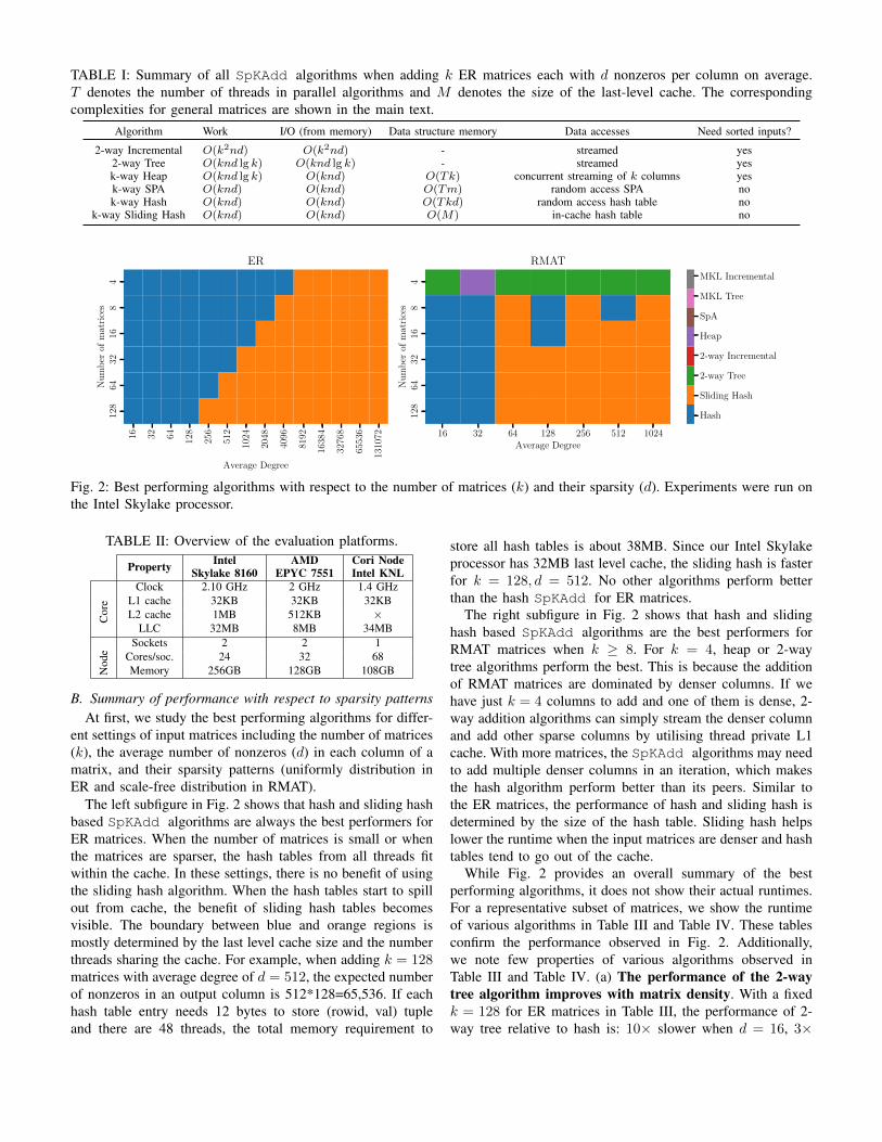
TABLE I: Summary of all SpKAdd algorithms when adding k ER matrices each with d nonzeros per column on average.T denotes the number of threads in parallel algorithms and M denotes the size of the last-level cache. The correspondingcomplexities for general matrices are shown in the main text.

Algorithm Work I/O (from memory) Data structure memory Data accesses Need sorted inputs?

2-way Incremental O(k2nd) O(k2nd) - streamed yes2-way Tree O(knd lg k) O(knd lg k) - streamed yesk-way Heap O(knd lg k) O(knd) O(Tk) concurrent streaming of k columns yesk-way SPA O(knd) O(knd) O(Tm) random access SPA nok-way Hash O(knd) O(knd) O(Tkd) random access hash table no

k-way Sliding Hash O(knd) O(knd) O(M) in-cache hash table no

16 32 64 128

256

512

1024

2048

4096

8192

1638

4

3276

8

6553

6

1310

72

Average Degree

48

1632

6412

8N

um

ber

ofm

atri

ces

ER

16 32 64 128 256 512 1024Average Degree

48

1632

6412

8N

um

ber

ofm

atri

ces

RMAT

Hash

Sliding Hash

2-way Tree

2-way Incremental

Heap

SpA

MKL Tree

MKL Incremental

Fig. 2: Best performing algorithms with respect to the number of matrices (k) and their sparsity (d). Experiments were run onthe Intel Skylake processor.

TABLE II: Overview of the evaluation platforms.

Property IntelSkylake 8160

AMDEPYC 7551

Cori NodeIntel KNL

Cor

e

Clock 2.10 GHz 2 GHz 1.4 GHzL1 cache 32KB 32KB 32KBL2 cache 1MB 512KB ×

LLC 32MB 8MB 34MB

Nod

e

Sockets 2 2 1Cores/soc. 24 32 68Memory 256GB 128GB 108GB

B. Summary of performance with respect to sparsity patternsAt first, we study the best performing algorithms for differ-

ent settings of input matrices including the number of matrices(k), the average number of nonzeros (d) in each column of amatrix, and their sparsity patterns (uniformly distribution inER and scale-free distribution in RMAT).

The left subfigure in Fig. 2 shows that hash and sliding hashbased SpKAdd algorithms are always the best performers forER matrices. When the number of matrices is small or whenthe matrices are sparser, the hash tables from all threads fitwithin the cache. In these settings, there is no benefit of usingthe sliding hash algorithm. When the hash tables start to spillout from cache, the benefit of sliding hash tables becomesvisible. The boundary between blue and orange regions ismostly determined by the last level cache size and the numberthreads sharing the cache. For example, when adding k = 128matrices with average degree of d = 512, the expected numberof nonzeros in an output column is 512*128=65,536. If eachhash table entry needs 12 bytes to store (rowid, val) tupleand there are 48 threads, the total memory requirement to

store all hash tables is about 38MB. Since our Intel Skylakeprocessor has 32MB last level cache, the sliding hash is fasterfor k = 128, d = 512. No other algorithms perform betterthan the hash SpKAdd for ER matrices.

The right subfigure in Fig. 2 shows that hash and slidinghash based SpKAdd algorithms are the best performers forRMAT matrices when k ≥ 8. For k = 4, heap or 2-waytree algorithms perform the best. This is because the additionof RMAT matrices are dominated by denser columns. If wehave just k = 4 columns to add and one of them is dense, 2-way addition algorithms can simply stream the denser columnand add other sparse columns by utilising thread private L1cache. With more matrices, the SpKAdd algorithms may needto add multiple denser columns in an iteration, which makesthe hash algorithm perform better than its peers. Similar tothe ER matrices, the performance of hash and sliding hash isdetermined by the size of the hash table. Sliding hash helpslower the runtime when the input matrices are denser and hashtables tend to go out of the cache.

While Fig. 2 provides an overall summary of the bestperforming algorithms, it does not show their actual runtimes.For a representative subset of matrices, we show the runtimeof various algorithms in Table III and Table IV. These tablesconfirm the performance observed in Fig. 2. Additionally,we note few properties of various algorithms observed inTable III and Table IV. (a) The performance of the 2-waytree algorithm improves with matrix density. With a fixedk = 128 for ER matrices in Table III, the performance of 2-way tree relative to hash is: 10× slower when d = 16, 3×

TABLE III: Runtime (sec) of different algorithms for different values of k and different average nonzeros per column (d) ofER matrices on the Intel Skylake processor (48 cores). Green cells represent the smallest runtime in each column.

Algorithm d = 16 d = 1024 d = 8192k = 4 k = 32 k = 128 k = 4 k = 32 k = 128 k = 4 k = 32 k = 128

2-way Incremental 0.0022 0.0316 0.4506 0.0357 0.6618 5.7806 0.1746 2.7200 could not runMKL Incremental 0.0588 0.6924 3.9971 0.1638 3.4144 29.1978 0.4717 12.9322 172.2600

2-way Tree 0.0019 0.0186 0.0832 0.0279 0.2440 1.2798 0.4416 0.8273 4.0545MKL Tree 0.0499 0.5237 2.2155 0.1425 1.8711 8.2814 0.4121 5.4968 26.1705

Heap 0.0037 0.0112 0.0374 0.0730 0.5570 2.1732 0.5914 4.5293 16.1049SPA 0.1237 0.1274 0.1309 0.1351 0.2844 0.8173 0.2579 1.3776 4.5269Hash 0.0007 0.0016 0.0083 0.0110 0.1362 0.4463 0.1312 0.8062 4.3987

Sliding Hash 0.0021 0.0045 0.0162 0.0272 0.0936 0.3330 0.0993 0.5773 1.8096

TABLE IV: Runtime (sec) of different algorithms for different values of k and different average nonzeros per column (d) ofRMAT matrices on the Intel Skylake processor (48 cores). Green cells represent the smallest runtime in each column.

Algorithm d = 16 d = 64 d = 512k = 4 k = 32 k = 128 k = 4 k = 32 k = 128 k = 4 k = 32 k = 128

2-way Incremental 0.1155 0.8078 3.1727 0.3269 2.4913 9.3310 2.1307 could not run could not runMKL Incremental 0.9839 6.0211 17.1921 3.5291 18.3133 47.9294 24.6052 109.5036 264.0963

2-way Tree 0.0774 0.2315 0.4691 0.2358 0.5673 0.9890 1.5213 3.3897 4.6937MKL Tree 0.8670 2.2720 4.1899 2.9447 5.9594 8.3661 19.8781 31.0663 33.3237

Heap 0.1371 0.1384 0.1960 0.2422 1.0980 0.7603 1.8223 3.5277 6.7888SPA 0.2467 0.2448 0.2386 0.5705 0.5659 0.6199 4.3047 4.6626 9.2565Hash 0.1068 0.0739 0.0719 0.3240 0.3121 0.2925 1.7651 1.8187 1.8500

Sliding Hash 0.1251 0.0794 0.0762 0.3206 0.2625 0.2562 1.7909 1.7053 1.5471

21 23 25

Number of threads

20

22

24

Tim

e(s

ec)

(a) ER, row=4M, col=1K,d=1024, k=128

21 23 25

Number of threads

22

24

26

Tim

e(s

ec)

(b) RMAT, row=4M, col=32K,d=512, k=128

21 23 25

Number of threads

2−1

21

23

25

Tim

e(s

ec)

(c) SpGEMM Intermediate matrices of Eukaryarow=3M, col=50K,

d=240, k=64

Hash Sliding Hash 2-way Tree MKL Tree SPA Heap

Fig. 3: Strong scaling of various SpKAdd algorithms on the Intel processor.

slower when d = 1024, and 1.1× faster when d = 8196.Similarly, for RMAT matrices with a fixed k = 128 inTable IV, the performance of 2-way tree relative to hash is:6× slower when d = 16, 3× slower when d = 1024, and2× slower when d = 8196. This is expected as hash tablesbecome larger for denser matrices, making the 2-way treealgorithm more efficient. However, the sliding hash algorithmis still the fastest at the extreme setting with d = 8196. (b)The SPA SpKAdd algorithm is as efficient as the hashSpKAdd algorithm for denser matrices as seen in the lastcolumn of Table III. This is expected because the hash tablesize (nnz(B(:, j))) becomes O(m) for dense output columns.This also suggests that the benefits of sliding hash can also beobserved in the SPA algorithm if we partition the SPA arraybased on row indices [16]. (c) 2-way SpKAdd using MKL issignificantly slower than other algorithms. The MKL-based2-way SpKAdd algorithms do not show promising results inour experiments. This especially true for larger values of k.

C. Scalability

We conducted the strong scaling experiments on the IntelSkylake processors with up to 48 threads (at most one threadper core). Fig. 3 shows the scalability results with (a) ER ma-trices, (b) RMAT matrices, and (c) 64 lower rank matrices gen-erated when running a distributed SpGEMM algorithm withthe Eukarya matrix. We observe that most algorithms scalealmost linearly except 2-way SpKAdd algorithms (MKL Treeand 2-way tree) and SPA-based SpKAdd . Our load balancingtechnique ensures that k-way SpKAdd implementations scalewell for matrices with skewed nonzero distributions. Theperformance of SPA suffers at high thread counts becauseof O(Tm) memory requirement where T is the number ofthreads and m is the number of rows in matrices. However, thesequential SPA-SpKAdd performs better than other algorithmson a single thread because a SPA with 4M entries can still fitin the cache that is not shared among threads. However, formatrices with more rows (e.g., more that 32M rows), SPAwould go out of cache even with a single thread.

27 29 211 213

Hash table size

0.02

0.04

0.06T

ime

(sec

)(a) ER, row=4M, col=1024,d=64, k=128, cf=1.00098,

machine=Skylake

28 211 214 217 220

Hash table size

2

4

6

8

Tim

e(s

ec)

(b) ER, row=4M, col=1024,d=8192, k=128, cf=1.12,

machine=Skylake

28 211 214 217 220

Hash table size

2

4

6

8

Tim

e(s

ec)

(c) RMAT, row=4M, col=32k,d=512, k=128, cf=1.25,

machine=Skylake

27 29 211 213 215

Hash table size

0.0

0.5

1.0

1.5

Tim

e(s

ec)

(d) Eukarya, row=3M, col=50K,d=240, k=64, cf=22.614,

machine=Skylake

28 211 214 217 220

Hash table size

5

10

15

Tim

e(s

ec)

(e) ER, row=4M, col=1024,d=8192, k=128, cf=1.12,

machine=EPYC

28 211 214 217 220

Hash table size

2

4

6

8

Tim

e(s

ec)

(f) RMAT, row=4M, col=32k,d=512, k=128, cf=1.25,

machine=EPYC

Symbolic Computation Total

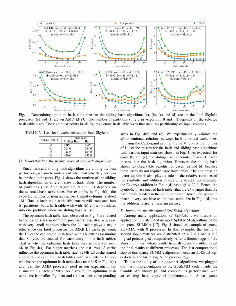
Fig. 4: Determining optimum hash table size for the sliding hash algorithm. (a), (b), (c) and (d) are on the Intel Skylakeprocessor. (e) and (f) are on AMD EPYC. The number of partitions (line 3 in Algorithm 8 and 7) depends on the selectedhash table sizes. The rightmost points in all figures denote hash table sizes that need no partitioning of input columns.

TABLE V: Last level cache misses on Intel Skylake.

Cases (Fig. 4) LL miss readSliding Hash Hash

(a) 1.8M 1.4M(b) 214M 734M(c) 344M 409M(d) 150M 152M

D. Understanding the performance of the hash algorithms

Since hash and sliding hash algorithms are among the bestperformers, we aim to understand when and why they performbetter than their peers. Fig. 4 shows the runtime of the slidinghash algorithm for different sizes of hash tables. The numberof partitions (line 3 in Algorithm 8 and 7) depends onthe selected hash table sizes. For example, in Fig. 4(b), theexpected number of nonzeros across k input columns is about1M. Thus, a hash table with 16K entries will translates into64 partitions, but a hash table with with 1M entries translatesinto one partition where no sliding hash is used.

The optimum hash table sizes observed in Fig. 4 are relatedto the cache sizes in different processors. Fig. 4(a) is a casewith very small matrices where the L1 cache plays a majorrole. Since our Intel processor has 32KB L1 cache per core,the L1 cache can hold a hash table with 4K entries (assumingthat 8 bytes are needed for each entry in the hash table).That is why the optimum hash table size is observed near4K in Fig. 4(a). For bigger matrices, the last level L3 cacheinfluence the optimum hash table size. 32MB L3 cache sharedamong threads can hold hash tables with 64K entries. Hence,we observe the optimum hash table sizes near 64K in Fig. 4(b)and (c). The AMD processor used in our experiment hasa smaller L3 cache (8MB). As a result, the optimum hashtable size is smaller Fig. 4(e) and (f) that their corresponding

sizes in Fig. 4(b) and (c). We experimentally validate theaforementioned relations between hash table and cache sizesby using the Cachegrind profiler. Table V reports the numberof LL cache misses for the hash and sliding hash algorithmswith various input matrices shown in Fig. 4. As expected, forcases (b) and (c), the sliding hash encounter fewer LL cachemisses than the hash algorithm. However, the sliding hashshows no observable benefits for cases (a) and (d) becausethese cases do not require large hash tables. The compressionfactor SpKAdd also plays a role in the relative runtimes ofthe symbolic and addition phases of spkadd. For example,the Eukarya addition in Fig. 4(d) has a cf = 22.6. Hence, thesymbolic phase needed hash tables that are 27× larger than thehash tables needed in the addition phase. Hence, the symbolicphase is very sensitive to the hash table size in Fig. 4(d), butthe addition phase remains insensitive.

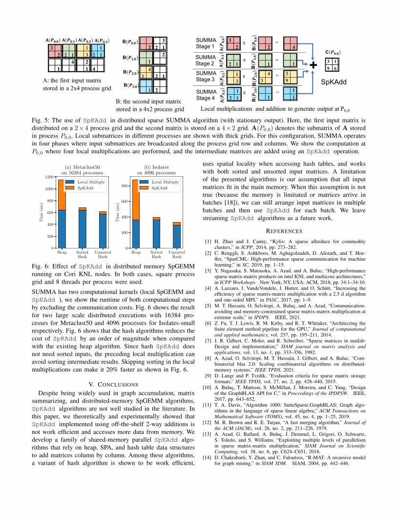
E. Impact on the distributed SpGEMM algorithmAmong many applications of SpKAdd , we discuss an

application in distributed memory SpGEMM algorithms basedon sparse SUMMA [17]. Fig. 5 shows an example of sparseSUMMA with 8 processes. In this example, the first andsecond input matrices are distributed on a 2 × 4 and 4 × 2logical process grids, respectively. After different stages of thealgorithm, intermediate results from all stages are added to getthe final results at different processes. The last computationalstep of this sparse SUMMA algorithm needs an SpKAdd op-eration as shown in Fig. 5 for process P0,0.

To test the utility of our SpKAdd algorithms, we pluggedour hash implementation in the SpGEMM code inside theCombBLAS library [8] and compare its performance withan existing heap SpKAdd implementation. Since sparse

1 13 2 121 4

32 2 1

41 4

3 2 1

1 2

32 2 1

21

32 2

2 1 1

13

43

12 1 1

x

x

x

x

4

1

39

11

=

=

=

=

3 19 6+

SpKAddA: the first input matrixstored in a 2x4 process grid

𝐀(𝑷𝟎,𝟎) 𝐀(𝑷𝟎,𝟑)𝐀(𝑷𝟎,𝟏) 𝐀(𝑷𝟎,𝟐) B(𝑷𝟎,𝟎)

B(𝑷𝟑,𝟎)

B(𝑷𝟏,𝟎)

B(𝑷𝟐,𝟎)

C(𝑷𝟎,𝟎)

𝐀(𝑷 𝟎

,𝟎)

B(𝑷

𝟎,𝟎)

𝐀(𝑷 𝟎

,𝟏)

𝐀(𝑷 𝟎

,𝟐)

𝐀(𝑷 𝟎

,𝟑)

B(𝑷

𝟏,𝟎)

B(𝑷

𝟐,𝟎)

B(𝑷

𝟑,𝟎)

B: the second input matrixstored in a 4x2 process grid

SUMMAStage 2

SUMMAStage 1

SUMMAStage 3

SUMMAStage 4

Local multiplications and addition to generate output at P0,0

Fig. 5: The use of SpKAdd in distributed sparse SUMMA algorithm (with stationary output). Here, the first input matrix isdistributed on a 2× 4 process grid and the second matrix is stored on a 4× 2 grid. A(P0,0) denotes the submatrix of A storedin process P0,0. Local submatrices in different processes are shown with thick grids. For this configuration, SUMMA operatesin four phases where input submatrices are broadcasted along the process grid row and columns. We show the computation atP0,0 where four local multiplications are performed, and the intermediate matrices are added using an SpKAdd operation.

Heap SortedHash

UnsortedHash

0

200

400

600

800

1000

1200

Tim

e(s

ec)

(a) Metaclust50on 16384 processes

Local Multiply

SpKAdd

Heap SortedHash

UnsortedHash

0

200

400

600

800

Tim

e(s

ec)

(b) Isolateson 4096 processes

Local Multiply

SpKAdd

Fig. 6: Effect of SpKAdd in distributed memory SpGEMMrunning on Cori KNL nodes. In both cases, square processgrid and 8 threads per process were used.

SUMMA has two computational kernels (local SpGEMM andSpKAdd ), we show the runtime of both computational stepsby excluding the communication costs. Fig. 6 shows the resultfor two large scale distributed executions with 16384 pro-cesses for Metaclust50 and 4096 processes for Isolates-smallrespectively. Fig. 6 shows that the hash algorithms reduces thecost of SpKAdd by an order of magnitude when comparedwith the existing heap algorithm. Since hash SpKAdd doesnot need sorted inputs, the preceding local multiplication canavoid sorting intermediate results. Skipping sorting in the localmultiplications can make it 20% faster as shown in Fig. 6.

V. CONCLUSIONS

Despite being widely used in graph accumulation, matrixsummarizing, and distributed-memory SpGEMM algorithms,SpKAdd algorithms are not well studied in the literature. Inthis paper, we theoretically and experimentally showed thatSpKAdd implemented using off-the-shelf 2-way additions isnot work efficient and accesses more data from memory. Wedevelop a family of shared-memory parallel SpKAdd algo-rithms that rely on heap, SPA, and hash table data structuresto add matrices column by column. Among these algorithms,a variant of hash algorithm is shown to be work efficient,

uses spatial locality when accessing hash tables, and workswith both sorted and unsorted input matrices. A limitationof the presented algorithms is our assumption that all inputmatrices fit in the main memory. When this assumption is nottrue (because the memory is limitated or matrices arrive inbatches [18]), we can still arrange input matrices in multiplebatches and then use SpKAdd for each batch. We leavestreaming SpKAdd algorithms as a future work.

REFERENCES

[1] H. Zhao and J. Canny, “Kylix: A sparse allreduce for commodityclusters,” in ICPP, 2014, pp. 273–282.

[2] C. Renggli, S. Ashkboos, M. Aghagolzadeh, D. Alistarh, and T. Hoe-fler, “SparCML: High-performance sparse communication for machinelearning,” in SC, 2019, pp. 1–15.

[3] Y. Nagasaka, S. Matsuoka, A. Azad, and A. Buluc, “High-performancesparse matrix-matrix products on intel KNL and multicore architectures,”in ICPP Workshops. New York, NY, USA: ACM, 2018, pp. 34:1–34:10.

[4] A. Lazzaro, J. VandeVondele, J. Hutter, and O. Schutt, “Increasing theefficiency of sparse matrix-matrix multiplication with a 2.5 d algorithmand one-sided MPI,” in PASC, 2017, pp. 1–9.

[5] M. T. Hussain, O. Selvitopi, A. Buluc, and A. Azad, “Communication-avoiding and memory-constrained sparse matrix-matrix multiplication atextreme scale,” in IPDPS. IEEE, 2021.

[6] Z. Fu, T. J. Lewis, R. M. Kirby, and R. T. Whitaker, “Architecting thefinite element method pipeline for the GPU,” Journal of computationaland applied mathematics, vol. 257, pp. 195–211, 2014.

[7] J. R. Gilbert, C. Moler, and R. Schreiber, “Sparse matrices in matlab:Design and implementation,” SIAM journal on matrix analysis andapplications, vol. 13, no. 1, pp. 333–356, 1992.

[8] A. Azad, O. Selvitopi, M. T. Hussain, J. Gilbert, and A. Buluc, “Com-binatorial blas 2.0: Scaling combinatorial algorithms on distributed-memory systems,” IEEE TPDS, 2021.

[9] D. Langr and P. Tvrdik, “Evaluation criteria for sparse matrix storageformats,” IEEE TPDS, vol. 27, no. 2, pp. 428–440, 2015.

[10] A. Buluc, T. Mattson, S. McMillan, J. Moreira, and C. Yang, “Designof the GraphBLAS API for C,” in Proceedings of the IPDPSW. IEEE,2017, pp. 643–652.

[11] T. A. Davis, “Algorithm 1000: SuiteSparse:GraphBLAS: Graph algo-rithms in the language of sparse linear algebra,” ACM Transactions onMathematical Software (TOMS), vol. 45, no. 4, pp. 1–25, 2019.

[12] M. R. Brown and R. E. Tarjan, “A fast merging algorithm,” Journal ofthe ACM (JACM), vol. 26, no. 2, pp. 211–226, 1979.

[13] A. Azad, G. Ballard, A. Buluc, J. Demmel, L. Grigori, O. Schwartz,S. Toledo, and S. Williams, “Exploiting multiple levels of parallelismin sparse matrix-matrix multiplication,” SIAM Journal on ScientificComputing, vol. 38, no. 6, pp. C624–C651, 2016.

[14] D. Chakrabarti, Y. Zhan, and C. Faloutsos, “R-MAT: A recursive modelfor graph mining,” in SIAM SDM. SIAM, 2004, pp. 442–446.

[15] A. Azad, A. Buluc, G. A. Pavlopoulos, N. C. Kyrpides, and C. A.Ouzounis, “HipMCL: a high-performance parallel implementation of theMarkov clustering algorithm for large-scale networks,” Nucleic AcidsResearch, vol. 46, no. 6, pp. e33–e33, 01 2018.

[16] M. M. A. Patwary, N. R. Satish, N. Sundaram, J. Park, M. J. Anderson,S. G. Vadlamudi, D. Das, S. G. Pudov, V. O. Pirogov, and P. Dubey,“Parallel efficient sparse matrix-matrix multiplication on multicore plat-forms,” in International Conference on High Performance Computing.Springer, 2015, pp. 48–57.

[17] A. Buluc and J. R. Gilbert, “Parallel sparse matrix-matrix multiplicationand indexing: Implementation and experiments,” SIAM Journal onScientific Computing, vol. 34, no. 4, pp. C170–C191, 2012.

[18] O. Selvitopi, M. T. Hussain, A. Azad, and A. Buluc, “Optimizinghigh performance Markov clustering for pre-exascale architectures,” inIPDPS, 2020.