Parabolic-elliptic systems with general density-pressure relations

31

Parabolic-elliptic systemswith general density-pressure relations

Piotr BILER, Robert STANCZYInstytut Matematyczny, Uniwersytet Wrodawski, pi. Grunwaldzki 2/4, 50-384 Wroclaw, Poland

Piotr.Biler , stanczr}@math.uni .wroc.pl

AbstractThis survey paper contains generalizations of results on the behavior of solutions

of particular systems describing the interaction of gravitationally attracting particlesthat obey either the Maxwell-Boltzmann or the Fermi-Dirac statistics.

Key words and phrases: generalized Chavanis-Sommeria-Robert model, mean fieldequation, nonlinear nonlocal parabolic system, steady states, blow up of solutions.

2000 Mathematics Subject Classi ication: $35\mathrm{Q}$ , $35\mathrm{K}60,35\mathrm{B}40$ , $82\mathrm{C}21$

1 Introduction and derivation of the systemWe study in this paper parabolic-elliptic systems of the form

$n_{t}$ $=$ $\nabla\cdot(D_{*}(\nabla p+n\nabla\varphi))$ , (1)$\Delta\varphi$ $=$ $n$ , (2)

which are considered in statistical mechanics as hydrodynamical models for self-interactingparticles. Here $n=n(x, t)\geq 0$ is the density function defined for (x) $t)\in\Omega\cross \mathbb{R}^{+}$ , $\Omega\subset \mathbb{R}^{d}$,$\varphi$ $=\varphi(x, t)$ is the Newtonian potential generated by the particles of density $n$ , and thepressure $p\geq 0$ is determined by the density-pressure relation with a sufficiently regular(say, $C^{2}(\mathbb{R}^{+}\cross \mathbb{R}^{+})$) function $p$

$p=p(n, \theta)$ . (3)

The parameter $\theta>0$ plays the role of the temperature, and $D_{*}>0$ is a coefficient whichmay depend on $n$ , $\mathrm{f}\mathrm{i}$ , $\mathrm{f}$ , $x$ , . . Such systems can be studied either in the canonicalensemble (i.e. the isothermal setting), when rt $=$ const is fixed, or in the microcanonicalensemble with a variable temperature: either $\theta=\theta(t)$ or t9 $=\theta(x, t)$ . Then, the energybalance is described either by a relation like

$E=c_{0} \int_{\Omega}pdx+\frac{1}{2}\int_{\Omega}n\varphi dx=$ const (4)

数理解析研究所講究録 1405巻 2004年 31-53

32

(which, for a given $n$ , defines $\theta=\theta(t)$ in an implicit way) in the former case, or by anevolution partial differential equation for $\theta$ $=\theta(x, t)$ as was in [26, 27, 6] in the latter case.Thus, $(1)-(2)$ can be viewed as evolution equations for self-consistent gravitational field Q.

In fact, the starting point of the derivation of related mean field models in astrophysicsin [17] consists of an analysis of kinetic equations whose evolution in time is governed bythe Maximum Entropy Production Principle. More precisely, if $0\leq f=f(x, v, t)$ is thedensity of particles at the point $(x, t)\in \mathit{7}\mathit{2}$

$\mathrm{x}\mathbb{R}^{+}$ , $\Omega\subset \mathbb{R}^{d}$ , moving at the velocity $v$ , then $f$

satisfies a kinetic equation

$f_{t}+v\cdot \mathit{7}_{x}f-\nabla\varphi\cdot \mathit{7}_{v}f=-$ $\mathrm{s}7v\mathrm{j}$

with a general dissipation flux term $-\nabla_{v}\mathrm{j}$ . Moreover, a priori an integral functional$S= \int_{\mathrm{R}^{d}}s$ ( $f$ (x, $v,$ $t$ )) $dv$ , called the local entropy, is given. Distribution functions $f$ thatmaximize this functional (under local density and pressure constraints, see (5), (6) below)have a particular form depending on some parameters A $=\lambda(x, t)$ , $\theta=\theta(t)$ , etc., see theexamples presented in Section 2. Then, the term Vvj is determined (up to a positivediffusion coefficient) by the requirement that the system evolves with maximal entropyproduction rate at each moment $t$ . Averaging $f$ over the velocities $v\in \mathbb{R}^{d}$ , and thenpassing to the limit of large friction (or large times) lead to “hydrodynamic” equations inthe $(x, t)$ space. For the details of that construction we refer to $[17, 16]$ and [7].Given the distribution $f$ on the kinetic level, the spati0-temporal density is

$n(x, t)=/$$d$

$f(x, v, t)dv$ , (5)

and the pressure is defined by

$p(x, t)= \frac{1}{d}\int_{\mathrm{R}^{d}}|v|^{2}f(x, v, t)dv$. (6)

Thus, the first term in the energy (4) corresponds to the kinetic energy of particles (withthe natural choice $c_{0}=d/2$ in (4) $)$ , and the second is the potential energy of the systemof self-gravitating particles. As we will see further, mild assumptions (26) on the form of$f$ lead to natural density-pressure relations between $n$ and $p$ , see (28).

We consider the system $(1)-(‘ 2)$ with the natural n0- lux boundary condition on an$(\nabla p+n\nabla\varphi)$ . $\overline{\nu}=0$ (7)

($\overline{\nu}$ is the unit exterior normal vector to $\partial\Omega$), and an initial condition

$n(x, 0)=n_{0}(x)\geq 0.$ (8)

We impose on the potential ? either a physically acceptable “free” condition

$l\mathit{2}$$=E_{d}\mathrm{E}$ $n$ , (9)

33

$E_{d}(z)=-((d-2)\sigma_{d})^{-1}|z|^{2-d}$ being the fundamental solution of the Laplacian in $\mathbb{R}^{d}$ , $d\geq 3,$

or the homogeneous Dirichlet boundary condition

$?|\partial\Omega$ $=0,$ (10)

which is mathematically somewhat simpler. In the case of radially symmetric solutions(10) is, however, equivalent to (9) which can be obtained by adding a constant to thepotential $\varphi$ , cf. the discussion of this issue in [8, 9, 3]. As a consequence of (7), total mass

$M= \int_{\Omega}n(x, t)dx$ (11)

is conserved during the evolution. Moreover, sufficiently regular solutions of the evolutionproblem with $n_{0}\geq 0$ remain positive.

The main mathematical questions concerning the system are the following:

$\circ$ existence, nonexistence and multiplicity of steady states, either for given $M$, $\theta$ or for$M$ , $E$ fixed,

$\circ$ local in time existence of solutions of the evolution problem,

$\circ$ asymptotics of global in time solutions,

$\circ$ possibility of finite time blow up of solutions (corresponding to either a gravitationalcollapse or an explosion).

Two systems with particular density-pressure relations have been recently studied: forBrownian (or Maxwell-Boltzmann) and for Fermi-Dirac particles.

The model of self-gravitating Brownian particles, which consists of $(1)-(2)$ , (13) below,supplemented by (4), has been considered in [17, 15, 19] for radially symmetric solutions$(n, \varphi)$ (with $c_{0}=d/2$), and in $[18, 10]$ without this symmetry assumption. Studies ofthe corresponding isothermal problem with $?\equiv 1$ had been conducted earlier, see e.g.$[8, 1]$ . However, the motivations there had been a bit different – stemming from statisticalmechanics of interacting charged particles in semiconductors, electrolytes, plasmas (seealso [4] and [21] for different density-pressure relations) with (2) replaced by $\Delta\varphi=-n$ ,and afterwards for gravitating particles. Besides the statistical mechanics, systems of theform $(1)-(2)$ appear also in modelling of chemotaxis phenomena in biology, generalizingthe classical approach of E. F. Keller and L. A. Segel which involved the linear diffusionwith $p=$ const $n$ . These biological models, supplemented by the homogeneous Neumannconditions for $n$ and ? are applicable in description of concentration of either cells ormicroorganisms due to chemical agents. We refer the reader to [20] for a comprehensivereview of these aspects of parabolic-elliptic systems like $(1)-(2)$ . The papers [15, 18, 10, 3, 9]deal with the Brownian particles models. The main issues are:

34

$\circ$ gravitational collapse is possible for $d\geq 2$ in the isothermal model and for $d\geq 3$ inthe nonisothermal model,

$\circ$ the existence of steady states with prescribed mass and energy in $d\geq 3$ dimensionsis controlled by the parameter $E/M^{2}$ which should be large enough.

Since the Fermi-Dirac model, see (17) below, involves nonlinear diffusion, even localin time existence of solutions is much harder to establish than in the Brownian (lineardiffusion) case, see [7] where in the isothermal case a specific choice of the coefficient$D_{*}$ has been considered. There are also many results on radially symmetric stationarysolutions in [12, 13, 14]. In particular:

$\circ$ structure of the set of steady states with given $M$ and $\theta$ is different (and less com-plicated) than in the Brownian case ([13]),

$\circ$ the existence of steady states with given mass and energy is controlled by the pa-rameter $\min\{\frac{E}{M}7, \frac{E}{M^{1+2/d}}\}([11,25])$ ,

$\circ$ gravitational collapse cannot occur in $d\leq 3$ dimensions in the isothermal case ([7]),

$\circ$ the gravitational collapse is possible for $d\geq 4$ for suitable initial data in the non-isothermal case ([11]).

We will study in this paper:

$\circ$ examples of density-pressure relations more general than Maxwell-Boltzmann andFermi-Dirac (in Section 2),

$\circ$ existence of entropy functionals and entropy production rates (in Section 3),

$\circ$ existence of steady states with prescribed mass and sufficiently large energy (in Sec-than 4),

$\circ$ nonexistence of global in time solutions of $(1)-(2)$ with general density-pressure rela-than$\mathrm{s}$ (3), $D_{*}=1,$ one of the conditions (9), (10), and either negative initial entropyor low energy (in Section 5), and thus, a fortiori, we obtain nonexistence of steadystates for arbitrary $D_{*}$ ,

$\circ$ continuation of local in time solutions of $(1)-(2)$ with polytropic density-pressurerelations (in Section 6).

We do not consider here the question of the local in time existence of solutions of theevolution problem which seems to be a rather difficult question (mainly because of nonlinearboundary conditions for $n$ and possible degeneracies of diffusion) in such a general settingwith (3), cf. the isothermal Fermi-Dirac case in [7]. Note that results for systems of

35

(several species of) repulsing particles with linear boundary conditions for $n$ are in themonograph [21].

It is worth noting that while “local” results on the existence of steady states (i.e. fora small range of control parameters $M$ , $\theta$ , $E$ ) are quite similar for general $p=p(n, \theta)$ ,see Th. 4.2 below, the global structure of the set of steady states is rather sensitive tovariations of the form of $p$ in (3), cf. results for the Boltzmann and Fermi-Dirac models.Notation. In the sequel $|$ . $|_{p}$ will denote the $L^{p}(\Omega)$ norm. The letter $C$ will denoteinessential constants which may vary from line to line.

2 Examples of density-pressure relationsIn this section recall some important distributions and density-pressure relations instatistical mechanics, generalize these examples, and formulate our assumptions on thestructure of the pressure function $p$ .2.1. Maxwell-Boltzmann distributionsThey are characterized by

f $=\lambda^{-1}e^{-|v|^{2}/2\theta}$ , (12)

where $A$ $=$ A $(x, t)>0$ is a physical parameter of fugacity, and t9 $=\theta(t)>0$ is aninstantaneous temperature uniform in $x$ . With some abuse of notation we will write $f=$$f(x, v, t)=f(\lambda, \theta, v)$ . These are maximizers of the Boltzmann entropy

$S= \frac{-1}{\int_{\mathrm{R}^{d}}fdv}\int_{\mathbb{R}^{d}}f\log fdv$ .

The corresponding macroscopic density and the pressure are

$n= \lambda^{-1}\sigma_{d}2^{d/2-1}\theta^{d/2}\Gamma(\frac{d}{2})$ . $p= \lambda^{-1}\sigma_{d}2^{d/2-1}\theta^{d/2+1}\Gamma(\frac{d}{2})$ ,

so that$p_{\mathrm{M}\mathrm{B}}(n, 9)$ $=On.$ (13)

This is the classical Boltzmann relation leading to linear (Brownian) diffusion term in (1).Indeed, $n(x, t)= \int_{1\mathrm{R}^{d}}\lambda^{-1}e^{-1}v|^{2}/2$’ $dv=\lambda^{-1}\mathrm{v}_{d}(2\mathrm{t}5)^{d/2}$ $\int_{0}^{\infty}e^{-r^{2}}rd-1dr$ , and $p$ is calculated ina similar manner.2.2. Fermi-Dirac distributionsThey have the form

$f= \frac{\eta_{0}}{\lambda e^{|v|^{2}/2\theta}+1}$ (14)

with a fixed $\eta_{0}>0,$ and again $\lambda=\lambda(x, t)>0$, $\theta=\theta(t)>0.$ They maximize the entropy

$S= \frac{-1}{\int_{\mathrm{R}^{d}}fdv}\int_{\mathrm{R}^{d}}$ ( $\frac{f}{\eta_{0}}\log\frac{f}{\eta_{0}}+$ $(1-4)$ $\log(1-\frac{f}{\eta_{0}})$ ) $dv$

3Ei

whose form a priori prevents from the overcrowding of particles at $(x, v, t):0\leq f\leq\eta 0.$

Then we have (see e.g. [15], [7, (1.1)-(1.3)])

$n=\eta_{0}2^{d/2-1}\sigma_{d}\theta^{d/2}I_{d/2-1}(\lambda)$ , $p= \eta_{0^{\underline{9}^{d/2}}}\frac{\sigma_{d}}{d}\theta^{d/2+1}I_{d/2}(\lambda)$, (15)

where $I_{\alpha}$ denotes the Fermi integral of order $\alpha>-1$ defined for all $\lambda>0$

$I_{\alpha}( \lambda)=\int_{0}$

”

$\frac{y^{\alpha}dy}{\lambda e^{y}+1}$ . (16)

Hence$p_{\mathrm{F}\mathrm{D}}(n, \theta)=\frac{\mu}{d}5^{d/2+1}$ $(I_{d/2} \circ I_{\overline{d/}2-1}^{1})(\frac{2}{\mu}\frac{n}{\theta^{d/2}})$ (17)

for a constant $\mu>0,$ which leads to a nonlinear diffusion in (1). Properties of Fermiintegrals (16) (convexity, asymptotics, etc.) relevant to study of the system $(1)-(2)$ arecollected in [7, Sec. 2] and [11, Sec. 5].

2.3. Bose-Einstein distributionsThey a $\mathrm{e}$ of the form

$f= \frac{\eta_{0}}{\lambda e^{|v|^{2}/2\theta}-1}$ (18)

with $\eta_{0}>0$ , $\lambda=\lambda(x, t)>1$ , $\theta=$ #(t) $>0.$ Similarly as before, we obtain

$p_{\mathrm{B}\mathrm{E}}(n, \theta)=\frac{\mu}{d}11^{d/2+1}$ $(J_{d/2}\circ J_{d/2-1}^{-1}$ ) $( \frac{2}{\mu}\frac{n}{\theta^{d/2}})$ , (19)

where $J_{\alpha}$ denotes the integral$J_{a}( \lambda)=\int_{0}^{\infty}\frac{y^{\alpha}dy}{\lambda e^{y}-1}$ (20)

defined either for $at>-1$ and $\lambda>1,$ or $\alpha>0$ and $\lambda\geq 1.$ Note that $\sup_{\lambda>1}J_{\alpha}(\lambda)$ is finiteif and only if $\alpha>0.$

Examples 2.2 and 2.3 are well known in quantum statistical mechanics of particles withspin: fermions and bosons, respectively.

2.4. tropic equations of stateThe distributions corresponding to polytropic equations of state of a gas on the kineticlevel have the form

$f=A( \alpha-\frac{|v|^{2}}{2})_{+}^{\frac{1}{q-1}}$ (21)

(or, more generally $f=A( \alpha-\varphi-\frac{|v|^{2}}{2})_{+}^{\frac{1}{q-1}}$ ), where $r_{+}= \max(r,0)$ , $q>1$ , $A=(\mathrm{L})^{\frac{1}{q-1}}q^{\frac{-1}{\theta}}$

’

$\alpha=\frac{1-(q-1)\lambda}{q-1}\theta$ with A $=\lambda(x, t)\in(-\infty, 1/(q-1))$ , t9 $=\theta(t)>0.$ They are obtained byextremizing the R\’enyi-Tsallis entropy

$S= \frac{-1}{q-1}\int_{\Omega \mathrm{x}\mathbb{R}^{d}}(f^{q}-f)dxdv$

37

$n\mathrm{a}\mathrm{t}$ $=A2^{d/2-1}\sigma_{d}\alpha^{\frac{\mathrm{d}1}{q-1}+\frac{d}{2}}B\mathrm{f}\mathrm{i}\mathrm{x}\mathrm{e}\mathrm{d}\mathrm{m}\mathrm{a}\mathrm{s}\mathrm{s}\mathrm{a}\mathrm{n}\mathrm{e}\mathrm{n}\mathrm{e}\mathrm{r}\mathrm{g}\mathrm{y}$

cf. [16].$\mathrm{A}\mathrm{f}\mathrm{t}\mathrm{e}\mathrm{r}\mathrm{i}\mathrm{n}\mathrm{t}\mathrm{e}\mathrm{g}\mathrm{r}\mathrm{a}\mathrm{t}\mathrm{i}\mathrm{n}\mathrm{g}\mathrm{w}\mathrm{i}\mathrm{t}\mathrm{r}\mathrm{e}\mathrm{s}\mathrm{p}\mathrm{e}\mathrm{c}\mathrm{t}p=A2^{d/2-\mathrm{l}}\sigma_{d}\alpha^{\frac{\mathrm{h}1}{q-1}+\frac{d}{2}+1}B(\begin{array}{ll} ||\frac{d}{2},1+ \frac{1}{q-1}\end{array}) \mathrm{t}\mathrm{o}r=v\mathrm{w}\mathrm{e}\frac{\mathrm{o}\mathrm{b}\mathrm{t}\mathrm{a}\mathrm{i}\mathrm{n}1}{\frac{d}{2}+\frac{1}{q-1}+1}$

,

where $B$ denotes the Euler Beta function $B(s, t)= \frac{\Gamma(s)\Gamma(t)}{\Gamma(s+t)}$ , see [16). Thus we arrive at therelation

$p_{1+\gamma}(n,\theta)=\kappa_{\gamma}\theta^{1-\gamma\frac{d}{2}}n^{1+\gamma}$ (22)

with $1/\gamma=1/(q-1)$ $+d/2>d/2$ , so that $q=1+ \frac{1}{1/\gamma-d/2}$ , and the polytropic constant

$\kappa_{\gamma}=\Delta\gamma+\overline{1}$ ($2^{d/2-1}\sigma_{d}B$ ( $\frac{d}{2}$ , $1$$\mathrm{t}$ $\frac{1}{\gamma}-\frac{d}{2}$)) $(1+ \frac{1}{\gamma}-\frac{d}{2})^{\gamma\frac{d}{2}-1}$ , since

$(^{q} \frac{-1}{q})^{\frac{1}{q-1}}=(1+\frac{1}{\gamma}-\frac{d}{2})^{\frac{1}{\gamma}-\frac{d}{2}}$ Passing to the limit $q\nearrow\infty$ , we have $\gamma=2/d$, and $p$ isindependent of $\theta$

$p_{1+2/d}(n, \theta)=\kappa_{2/d}n^{1+2/d}$ . (23)

The limit case $q\mathrm{s}$$1$ corresponds to the Boltzmann density-pressure relation (13), cf. also

the limit Boltzmann entropy $S$ .Remark. The Fermi-Dirac model results, in certain sense, as an interpolation betweenmean field models involving the Brownian diffusion and diffusion in gases. In the classicallimit $\lambda/$ oo (i.e. $n/\theta^{d/2}\backslash$ 0, e.g. for fixed $\theta>0$ and the small density $narrow 0$) therelation

$\frac{p_{\mathrm{F}\mathrm{D}}}{n}=\frac{2}{d}\mathrm{y}$ $\frac{I_{d/2}(\lambda)}{I_{d/2-1}(\lambda)}\sim y$ (24)

holds. This limit corresponds to the linear Brownian diffusion as was in [15, 10, 18]. Thecompletely degenerate case (white dwari in astrophysics), A $\mathrm{s}$ $0$ (i.e. $n/\theta^{d/2}\nearrow\infty$ , e.g.for $\theta>0$ fixed, and the large density $narrow\infty$ ), corresponds to the relation

$\frac{p_{\mathrm{F}\mathrm{D}}}{n^{1+2/d}}\sim\frac{2}{d+2}$,

$\frac{d}{\mu}$ )$2/d$

$=\kappa=$ const, (25)

i.e., to a polytropic equation of state of a gas.Note that the distribution function $f$ in (21) can be written using $n$ , $\theta$ and $v$ as

$f=C_{d,\gamma}(( \frac{n}{\theta^{d/2}})^{\gamma}-\frac{\gamma}{(\gamma+1)\kappa_{\gamma}}\frac{|v|^{2}}{2\theta})_{+}^{1/\gamma-d/2}$

These polytropic relations define evolution equations with nonlinear diffusions as, e.g.,in the porous media equation.

There are also other relevant density-pressure relations including nonlocal ones con-sidered in [5] and references therein, and leading to linear diffusions defined by pseudodif-ferential operators of L\’evy-Khinchin type so that the associated stochastic processes havediscontinuous trajectories.

In the examples $2.1-2\mathrm{A}$ the scaling relation$f(\lambda, \theta, \theta^{1/2}v)\equiv f(\lambda, 1, v)$ (26)

38

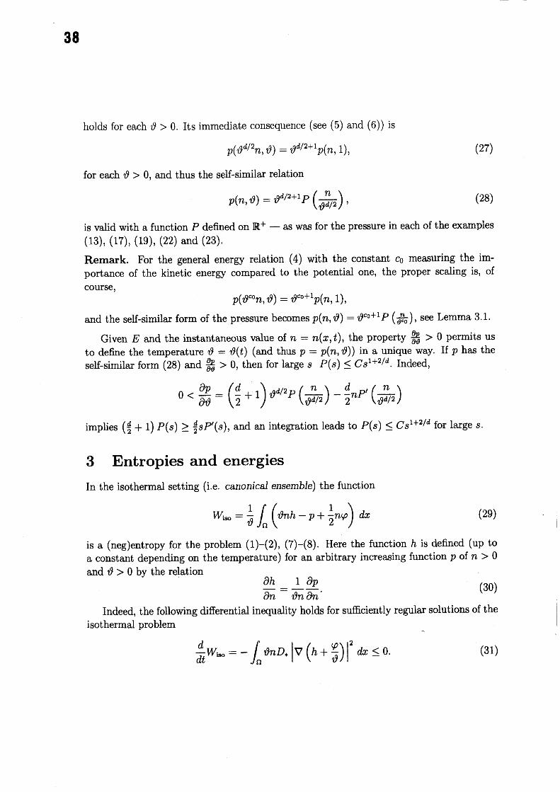
holds for each $\theta>0.$ Its immediate consequence (see (5) and (6)) is

$p(\theta^{d/2}n, 2)$ $=7^{d/2+1}p(n, 1)$ , (27)

for each $\theta>0,$ and thus the self-similar relation

$p(n, 7)$ $= \theta^{d/2+1}P(\frac{n}{\theta^{d/2}})$ , (28)

i $\mathrm{s}$ valid with a function $P$ defined on $\mathbb{R}^{+}-$ as was for the pressure in each of the examples(13), (17), (19), (22) and (23).

Remark. For the general energy relation (4) with the constant $c_{0}$ measuring the im-portance of the kinetic energy compared to the potential one, the proper scaling is, ofcourse,

$p(\theta^{c0}n, 9)$ $=\theta^{c\mathrm{o}+1}p(n, 1)$ ,

and the self-similar form of the pressure becomes $p(n, \theta)=\theta^{c_{0}+1}P(\frac{n}{\theta^{\mathrm{c}}0})$ , see Lemma 3.1.

Given $E$ and the instantaneous value of $n=n(x, t)$ , the property $\frac{\theta p}{\partial\theta}>0$ permits usto define the temperature t7 $=\theta(t)$ (and thus $p=p$($n$ , $\theta$)) in a unique way. If $p$ has theself-similar form (28) and $\mathrm{p}\partial\partial\theta>0,$ then for large $sP(s)\leq Cs^{1+2/d}$ . Indeed,

$0< \frac{\partial p}{\partial\theta}=(\frac{d}{2}+1)\theta^{d/2}P(\frac{n}{\theta^{d/2}})-\frac{d}{2}nP$’

$( \frac{n}{\theta^{d/2}})$

implies $( \frac{d}{2}+1)P(s)\geq\frac{d}{2}sP’(s)$ , and an integration leads to $P(s)$ $\leq Cs^{1+2/d}$ for large $s$ .

3 Entropies and energiesIn the isothermal setting (i.e. canonical ensemble) the function

$W_{\mathrm{i}\mathrm{s}\mathrm{o}}= \frac{1}{\theta}\int_{\Omega}$ ($\theta nh-p$ $+ \frac{1}{2}n\varphi$ ) $dx$ (29)

is a $(\mathrm{n}\mathrm{e}\mathrm{g})\mathrm{e}\mathrm{n}\mathrm{t}\mathrm{r}\mathrm{o}\mathrm{p}\mathrm{y}$ for the problem $(1)-(2)$ , $(7)-(8)$ . Here the function $h$ is defined (up toa constant depending on the temperature) for an arbitrary increasing function $p$ of $n>0$

and $\theta>0$ by the relation$\frac{\partial h}{\partial n}=\frac{1}{\theta n}.\frac{\partial p}{\partial n}$ , (30)

Indeed, the following differential inequality holds for sufficiently regular solutions of theisothermal problem

$\frac{d}{dt}W_{\mathrm{i}\mathrm{s}\mathrm{o}}=-\int_{\Omega}\theta nD_{*}|\nabla(h+\frac{\varphi}{\theta})|^{2}dx\leq 0$ . (31)

38

This is obtained multiplying (1) by $(h\mathrm{f}\varphi/\theta)$ , integrating by parts using the n0-fluxcondition (7), and noting that $\frac{\partial}{\partial n}(nh-\frac{p}{\theta})=h,$ $\frac{d}{dt}(\frac{1}{2}\int_{\Omega}n\varphi dx)=\int_{\Omega}\frac{dn}{dt}$ ’ $dx$ .

In the nonisothermal setting (i.e. microcanonical ensemble) the existence of a nontrivialentropy needs an assumption on the structure of $p$ in (3), i.e. on the dependence on $\theta$ .A simple sufficient condition is (28).

(32)

Lemma 3.1 If for the density-pressure relation (3) the condition $(\mathit{2}S)$ is satisfied witha function $P\in C^{1}$ , then

$W= \int_{\Omega}(nh-(\frac{d}{2}+1)\frac{p}{\theta})dx$

is an entropy for the problem $(\mathit{1})-(\mathit{2})$ , $(7)-(\mathit{8})$ , one of the boundary condition (9) or (10),with the energy relation (4), $c_{0}=d/2$ . Moreover, the following production of entropyformula holds

$\frac{d}{dt}W=-\int_{\Omega}\theta nD_{*}|\nabla(h+\frac{\varphi}{\theta})|^{2}dx\leq 0.$ (33)

Proof. Note that $p\in C^{2}$ is required in order to have (1) defined classically. However, weonly need $P\in C^{1}$ in the following calculations.

Observe that $W=W_{\mathrm{i}\mathrm{s}\mathrm{o}}-E/\theta$ . Let us compute $\frac{d}{dt}$ ( $\frac{1}{\theta}/*$ j. $dx$ ) in two ways.First, using the energy relation (4) and denoting $\frac{d}{dt}\theta$ by $\theta$ , we obtain

$\frac{d}{dt}(\frac{d}{2}\frac{1}{\theta}\int_{\Omega}pdx)$ $=$ $\frac{1}{\theta}\frac{d}{dt}(\frac{d}{2}\int_{\Omega}pdx)-\frac{d}{2}\frac{\dot{\theta}}{\theta^{2}}\int_{\Omega}pdx$

$=$ $\frac{1}{\theta}\frac{d}{dt}(E-\frac{1}{2}\int_{\Omega}n\varphi dx)-\frac{d}{2}\frac{\dot{\theta}}{\theta^{2}}\int_{\Omega}pdx$

$=$ $- \frac{1}{\theta}\int_{\Omega}n_{t}\varphi dx-\frac{d}{2}\frac{\dot{\theta}}{\theta^{2}}\Omega$$pdx$ .

Second, since by (28) the relation $p \partial\partial\theta=(\frac{d}{2}+1)R-\theta\frac{d}{2}\frac{n}{\theta}\frac{\partial p}{\partial n}$ holds, we have

$\frac{d}{dt}(\frac{1}{\theta}\int_{\Omega}pdx)$ $=$ $\frac{1}{\theta}\int_{\Omega}\frac{\partial p}{\partial n}n_{t}dx+\frac{\dot{\theta}}{\theta}\int_{\Omega}\frac{\partial p}{\partial\theta}dx-\frac{\dot{\theta}}{\theta^{2}}\int_{\Omega}pdx$

$=$ $\frac{1}{\theta}\int_{\Omega}.\frac{\partial p}{\partial n}n_{t}dx-\frac{d}{2}\frac{\dot{\theta}}{\theta^{2}}\int_{\Omega}n\frac{\partial p}{\partial n}dx\mathrm{f}$ $\frac{d}{2}\frac{\dot{\theta}}{\theta^{2}}\int_{\Omega}pdx$ .

Now we get

$\frac{d}{dt}W$ $=$ $\int_{\Omega}n_{t}hdx+\int_{\Omega}nh_{t}dx+\frac{1}{\theta}\int_{\Omega}ntydx+\frac{d}{2}\frac{\dot{\theta}}{\theta^{2}}\int_{\Omega}pdx$

$- \frac{1}{\theta}\int_{\Omega}\frac{\partial p}{\partial n}n_{\mathrm{t}}dx+\frac{d}{2}\frac{\dot{\theta}}{\theta^{2}}\int_{\Omega}n\frac{\partial p}{\partial n}dx$ $- \frac{d}{2}\frac{\dot{\theta}}{\theta^{2}}\int_{\Omega}p$ dx.

40

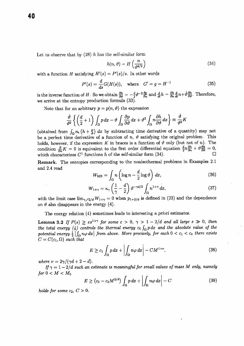
Let us observe that by (28) $h$ has the self-similar form

$h(n, \theta)=H(\frac{n}{\theta^{d/2}})$ (34)

with a function $H$ satisfying $H’(s)=P’(s)/s$ . In other words

$P’(s)=$ $\mathrm{B}G(H(s))$ , where $G’=g=H^{-1}$ (35)

$\mathrm{w}\mathrm{e}\mathrm{a}\mathrm{r}\mathrm{r}\mathrm{i}\mathrm{v}\mathrm{e}\mathrm{a}\mathrm{t}\mathrm{t}\mathrm{h}\mathrm{e}\mathrm{e}\mathrm{n}\mathrm{t}\mathrm{r}\mathrm{o}\mathrm{p}\mathrm{y}\mathrm{p}\mathrm{r}\mathrm{o}\mathrm{d}\mathrm{u}\mathrm{c}\mathrm{t}\mathrm{i}\mathrm{o}\mathrm{n}\mathrm{f}\mathrm{o}\mathrm{r}\mathrm{m}1’ \mathrm{a}(33\mathrm{i}\mathrm{s}\mathrm{t}\mathrm{h}\mathrm{e}\mathrm{i}\mathrm{n}\mathrm{v}\mathrm{e}\mathrm{r}\mathrm{s}\mathrm{e}\mathrm{f}\mathrm{u}\mathrm{n}\mathrm{c}\mathrm{t}\mathrm{i}\mathrm{o}\mathrm{n}\mathrm{o}\mathrm{f}H.\mathrm{S}\mathrm{o}\mathrm{w}\mathrm{e}\mathrm{o}\mathrm{b}\mathrm{t}\mathrm{a}\mathrm{i}\mathrm{n}\frac{\partial h}{\mathrm{u}\partial\theta}=-\frac{d}{)2}.\theta_{\partial n}^{-2\mathrm{g}}$

and $\frac{d}{dt}h=\frac{\partial h}{\partial n}\frac{d}{dt}n+\dot{\theta}\frac{\partial h}{\partial\theta}$ . Therefore,

Note that for an arbitrary $p=p(n, \theta)$ the expression

$\frac{\dot{\theta}}{\theta^{2}}\{(\frac{d}{2}+1)\int_{\Omega}pdx-\theta f_{\Omega}\frac{\partial p}{\partial\theta}dx+\theta^{2}\int_{\Omega}n\frac{\partial h}{\partial\theta}dx\}\equiv\frac{\theta}{\theta^{2}}K$

(obtained from $\int_{\Omega}n_{t}(h+\mathrm{E})\theta dx$ by subtracting time derivative of a quantity) may notbe a perfect time derivative of a function of $n$ , $\theta$ satisfying the original problem. Thisholds, however, if the expression $K$ in braces is a function of 19 only (but not of $n$ ). Thecondition $\frac{\partial}{\partial n}K=0$ is equivalent to the first order differential equation $\frac{d}{2}n\frac{\partial h}{\partial n}+$ $\mathrm{y}\frac{\partial h}{\partial\theta}=0,$

which characterizes $C^{1}$ functions $h$ of the self-similar form (34). $\square$

Remark. The entropies corresponding to the nonisothermal problems in Examples 2.1and 2.4 read

$W_{\mathrm{M}\mathrm{B}}$ $= \int_{\Omega}n(\log n-\frac{d}{2}\log\theta)dx$, (36)

$W_{1+\gamma}= \kappa_{\gamma}.(\frac{1}{\gamma}-\frac{d}{2})\theta^{-\gamma d/2}\int_{\Omega}n^{1+\gamma}dx$ , (37)

with the limit case $\lim_{\gamma\nearrow 2/d}W_{1+\gamma}=0$ when $p_{1+2/d}$ is defined in (23) and the dependenceon $\theta$ also disappears in the energy (4).

The energy relation (4) sometimes leads to interesting a priori estimates.

Lemma 3.2 If $P(s)\geq\epsilon s^{1+\gamma}$ for some $\epsilon$ $>0,$ $\gamma>1-2/d$ and all large $s\gg 0,$ thenthe total energy (4) controls the thermal energy $c_{0} \int_{\Omega}$ pclx and the absolute value of thepotential energy $\frac{1}{2}|\int_{\Omega}n\varphi dx|$ from above. More precisely, for each $0<c_{1}<c_{0}$ there exists$C=C(c_{1}, \Omega)$ such that

$E \geq c_{1}\int_{\Omega}pdx+|\mathit{1}_{\Omega}n\varphi dx|-CM^{1+}$’: (38)

$t$ here $\nu$ $=2\gamma/(\gamma d42-d)$ .If $\gamma=1-2/d$ such an estimate is meaningful for small values of mass $M$ only, namely

for $0<M<M_{0}$

$E \geq(c_{0}-c_{2}M^{2/d})\int_{\Omega}pdx+|\int_{\Omega}n\varphi dx|-C$ (39)

holds for some $c_{2}$ , $C>0.$

41

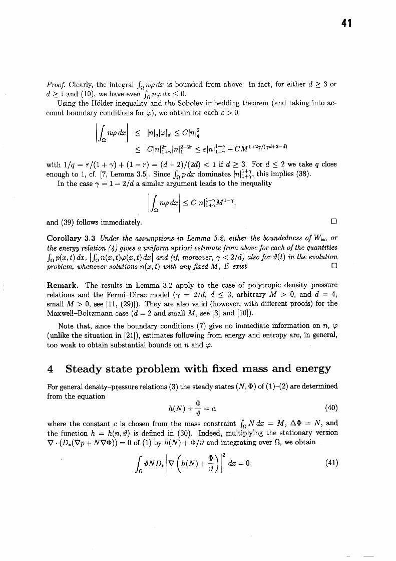
Proof. Clearly, the integral $\int_{\Omega}n\varphi dx$ is bounded from above. In fact, for either $d\geq 3$ or$d\geq 1$ and (10), we have even $\int_{\Omega}n\varphi dx\leq 0.$

Using the Holder inequality and the Sobolev imbedding theorem (and taking into ac-count boundary conditions for $\varphi$), we obtain for each $\epsilon>0$

$| \int_{\Omega}n\varphi dx|$ $\leq$ $|n|_{q}|\varphi|_{q’}\leq C|n|_{q}^{2}$

$\leq$ $C|n|_{1+\gamma}^{2r}|n|_{1}^{2-2r}\leq\epsilon|n|_{1+\gamma}^{1+\gamma}+CM^{1+2\gamma/(\gamma d+2-d)}$

with $1/q=r/(1+\gamma)+(1-r)=(d+2)/(2d)<1$ if $d\geq 3.$ For $d\leq 2$ we take $q$ closeenough to 1, cf. [7, Lemma 3.5]. Since $\int_{\Omega}pdx$ dominates $|n|_{1+\gamma}^{1+\gamma}$ , this implies (38).

In the case $\gamma$ $=1-2/d$ a similar argument leads to the inequality

$| \int_{\Omega}n\varphi dx|\leq C|n|_{1+\gamma}^{1+\gamma}M^{1-\gamma}$ ,

and (39) follows immediately. $\mathrm{C}1$

Corollary 3.3 Under the assumptions in Lemma 3.2, either the boundedness of $W_{\mathrm{i}\mathrm{s}\mathrm{o}}$ orthe energy relation (4) gives a uniform apriori estimate from above for each of the quantities$\int_{\Omega}p(x, t)dx$ , $|$ $/\Omega n(x, t)\varphi(x, t)dx|$ and ($\iota^{i}f_{f}$ moreover, $\gamma<2/d$) also for $\theta(t)$ in the evolutionproblem, whenever solutions $n(x, t)$ with any fixed $M$ , $Ee\dot{m}$ $t$ . $\square$

Remark. The results in Lemma 3.2 apply to the case of polytropic density-pressurerelations and the Fermi-Dirac model ($\gamma=2/d$ , $d\leq 3,$ arbitrary $M>0,$ and $d=4,$small $M>0,$ see [11, (29)] $)$ . They are also valid (however, with different proofs) for theMaxwell-Boltzmann case ($d=2$ and small $M$ , see [3] and [10]).

Note that, since the boundary conditions (7) give no immediate information on $n$ , $\varphi$

(unlike the situation in [21]), estimates following from energy and entropy are, in general,too weak to obtain substantial bounds on $n$ and 2.

4 Steady state problem with fixed mass and energy

For general density-pressure relations (3) the steady states $(N, \Phi)$ of $(1)-(2)$ are determinedfrom the equation

$h(N)+ \frac{\Phi}{\theta}=c,$ (40)

where the constant $c$ is chosen from the mass constraint $\int_{\Omega}Ndx=M$ , $\Delta I$ $=N,$ andthe function $h=h(n, \theta)$ is defined in (30). Indeed, multiplying the stationary version$\nabla\cdot(D_{*}(\nabla p+N\nabla\Phi))=0$ of (1) by $h(N)+\Phi/\mathrm{t}9$ and integrating over $\Omega$ , we obtain

$\int_{\Omega}\theta ND_{*}|\nabla$ ($h(N)$ $+ \frac{\Phi}{\theta}$ ) $|^{2}dx=0,$ (41)

42

which implies (40).Whenever $h$ is of self-similar form (34), the equation (40) can be written as

-t96$\Psi=\theta^{d/2}g(\Psi+c)$ , (42)

where $\Psi=-4\mathrm{I}?/\mathrm{t}9$ and $g=H^{-1}$ as in (35). Then, mass normalization becomes

$\theta^{d/2-1}\int_{\Omega}g(\Psi+c)dx=\frac{M}{\theta}$ . (43)

The energy constraint (4) with $c_{0}=d/2$ is now

$E= \mathit{7}_{2}^{d}\int_{\Omega}pd_{X}-\frac{\theta}{2}I_{\Omega}^{N\Psi d_{X}}$ . (44)

Entropies give an alternative way to derive and solve the equation (40) for steady

states. Namely, the production of entropy formula leads to (40) as was in the Browniancase studied in $[3, 9]$ and the Fermi-Dirac one in $[7, 11]$ . Moreover, we can use the entropy

$W_{\mathrm{i}\mathrm{s}\mathrm{o}}\mathrm{I}$ for the isothermal problem to obtain steady states as global minimizers of $W_{\mathrm{i}\mathrm{s}\mathrm{o}}$ . Thisis possible for $P(s)\geq Cs^{1+\gamma}$ with $\gamma$ $\geq 1-2/d$ . Using Lemma 3.2 we get relative weakcompactness of minimizing sequences for $W\mathrm{i}_{\mathrm{s}\mathrm{o}}$ considered on the set $\{W_{\mathrm{i}\mathrm{s}\mathrm{o}}\leq W0<\infty\}$ ,and $W_{\mathrm{i}\mathrm{s}\mathrm{o}}$ satisfies usual weak lower semicontinuity properties.

The second variational approach is possible via an analysis of the dual functional aswas in [28]. Without entering into the details (cf. [7, Sec. 4.1]), we recall that this givesfor each $M>0$ and $\theta>0,$ solvability of (42) supplemented with the Dirichlet condition(10) and mass constraint expressed as $\int_{\partial\Omega}\frac{\partial\Psi}{\partial\overline{\nu}}d\sigma=-M/\theta$ , whenever $P(s)\sim Cs^{1+\gamma}$ forlarge $s>0$ with $\gamma>1-2/d$ . Indeed, then $H(s)\sim Cs^{\gamma}$ , so $g(s|)$ $=H^{-1}(s)\sim Cs^{1/\gamma}$ , andthe sufficient condition in [28] reads $\lim_{sarrow\infty}g(s)/s^{p^{*}}=0$ for $p^{*}=d/(d-2)$ if $d\geq 3$ or$p^{*}<$ oo if $d=2.$ This is, of course, $1/\gamma<d/(d-2)$ , i.e. the same condition as before forminimization of $\mathrm{V}_{\mathrm{i}\mathrm{s}\mathrm{o}}$ .

Summarizing, we get for t9 $=$ const and either of the boundary conditions (9), (10),the following existence results similar to those in Propositions 4.1, 4.2 in [11].

Proposition 4.1 Under the assumption $P(s)\geq\epsilon s^{1+\gamma}$ with $\gamma>1-2/d$ and large $s>>0$

(as in Lemma 3.2), given $M>0$ there exists at least one solution $\Psi$ of the equation (42)

satisfying the condition (9) and (43). A similar result holds true for the case of boundarycondition (10). If $\gamma$ $=1-2/d$ those solutions exist for sufficiently small $M>0.$ $\square$

The question of the existence of multiple solutions of the equation (41), and theirstability as solutions of the evolution problem $(1)-(8)$ , is rather delicate. The problemis relatively well understood in the case of the Boltzmann model, cf. [3] and referencestherein. There are some numerical results in the case of radially symmetric solutions ofthe Fermi-Dirac model in the ball of $\mathbb{R}^{3}$ in [12, 13, 14].

43

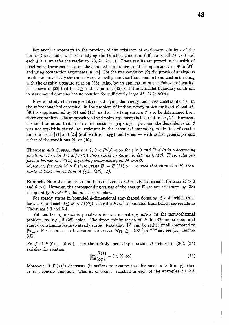
For another approach to the problem of the existence of stationary solutions of theFermi-Dirac model with 1 satisfying the Dirichlet condition (10) for small $M>0$ andeach $d\geq 3,$ we refer the reader to [23, 24, 25, 11]. These results are proved in the spirit offixed point theorems based on the compactness properties of the operator $N\mapsto\Psi$ in [23],and using contraction arguments in [24]. For the free condition (9) the proofs of analogousresults are practically the same. Here, we will generalize these results to an abstract settingwith the density-pressure relation (28). Also, by an application of the Pohozaev identity,it is shown in [23] that for $d\geq 5,$ the equation (42) with the Dirichlet boundary conditionin star-shaped domains has no solution for sufficiently large $M$ , $M\geq M(\theta)$ .

Now we study stationary solutions satisfying the energy and mass constraints, i.e. inthe microcanonical ensemble. In the problem of finding steady states for fixed $E$ and $M$ ,(40) is supplemented by (4) and (11), so that the temperature 19 is to be determined fromthese constraints. The approach via fixed point arguments is like that in $[23, 24]$ . However,it should be noted that in the aforementioned papers $p=p_{\mathrm{F}\mathrm{D}}$ and the dependence on $\theta$

was not explicitly stated (as irrelevant in the canonical ensemble), while it is of crucialimportance in [11] and [25] (still with $p=p_{\mathrm{F}\mathrm{D}}$) and herein – with rather general $p$’s andeither of the conditions (9) or (10).

Theorem 4.2 Suppose that $d\geq 2,$ $0<P’(s)<$ oo for $s\geq 0$ and $P’(s)/s$ is a decreasingfunction. Then for $0<M/\theta<<1$ there exists a solution of (42) with (43). These solutionsform a branch in $L^{\infty}(\Omega)$ depending continuously on $M$ and 19.Moreover, for each $M>0$ there exists $E_{0}=E_{0}(M)>$ $-\circ \mathrm{p}$ such that given $E>E_{0}$ thereeists at least one solution of (42), (43), (4).

Remark. Note that under assumptions of Lemma 3.2 steady states exist for each $M>0$

and $\theta>0.$ However, the corresponding values of the energy $E$ are not arbitrary: by (38)the quantity $E/M^{1+\nu}$ is bounded from below.

For steady states in bounded $d$-dimensional star-shaped domains, $d\geq 4$ (which existfor $\theta>0$ and each $0\leq M<M(\theta))$ , the ratio $E/M^{2}$ is bounded from below, see results inTheorems 5.3 and 5.4.

Yet another approach is possible whenever an entropy exists for the nonisothermalproblem, so, e.g., if (28) holds. The direct minimization of $W$ in (32) under mass andenergy constraints leads to steady states. Note that $|$ T4 $|$ can be rather small compared to

$|W_{\mathrm{i}\mathrm{s}\mathrm{o}}|$ . For instance, in the Fermi-Dirac case $W_{\mathrm{F}\mathrm{D}}\geq-C\theta$ $\int_{\Omega}n^{1-2/d}$ dx, see [11, Lemma3.5].

proofs If $P’(\mathrm{O})$ $\in(0, \infty)$ , then the strictly increasing function $H$ defined in (30), (34)satisfies the relation

$\lim\underline{H(s)}=\ell\in(0, \infty)$ . (45)$sarrow 0\log s$

Moreover, if $P’(s)/s$ decreases (it suffices to assume that for small $s>0$ only), then$H$ is a concave function. This is, of course, satisfied in each of the examples 2.1-2.3,

44

see $[7, 11]$ for the Fermi-Dirac case. Since $g=H^{-1}$ is a convex function, the function$g$ defined in (35), as well as its derivative $g’$ , are strictly increasing on $(-\infty, 0)$ with$\mathrm{g}(\mathrm{z})\sim\ell g’(z)\sim$ const $e^{z/\ell}$ , $zarrow-\infty$ .

Using this together with the positivity of $\Psi$ , we get from (43)

$c \leq g^{-1}(\frac{M}{\theta^{d}\mathit{1}^{2}|\Omega|})$ (46)

Moreover, for any $\Psi$ $\in L^{\infty}(\Omega)$ there exists a unique value $c$ satisfying (43), which we willdenote $c(\Psi)$ . The function $c$ is Lipschitz continuous: $|c($’ $1)-c(\Psi_{2})|\leq|$ I $1-\mathrm{I}$ $2|_{\infty}$ by (43)

and the mean value theorem, cf. [23, (1.11)]. Thus, looking for a solution of the problem(42)-(43) is reduced to finding a fixed point of the integral operator

$\mathrm{i}(\Psi)=\theta^{d/2-1}(-\Delta)^{-1}(g(\Psi+c(\Psi)))$ . (47)

Here $(-\Delta)^{-1}$ denotes the inverse of $-\mathrm{A}$ with an appropriate boundary condition, definedeither by the Green function of 0 or by the convolution with the fundamental solution.Its norm, as the operator considered in $L^{\infty}(\Omega)$ , is denoted by $A$ . Applying the meanvalue theorem for the function $g$ and monotonicity properties of 9 and $g’$ , we see that theLipschitz constant $L(M,\theta)$ of 7 on the unit ball $B(0,1)\subset L^{\infty}(\Omega)$ satisfies the estimate

$L(M, \theta)\leq 2A\theta^{d/2-1}g’(1+g^{-1}(\frac{M}{\theta^{d/2}|\Omega|}))$ (48)

Moreover, $\mathcal{T}$ maps the ball $B(0,1)$ into itself provided the inequality

$A \theta^{d/2-1}g(1+g^{-1}(\frac{M}{\theta^{d/2}|\Omega|}))\leq 1,$ (49)

holds. Since $1-d/2\leq 0,$ we conclude from (45), (48) that for sufficiently large $\theta$ : $0<$

$M/\theta\ll 1,$ say $M/\theta\leq m_{0}$ , the conditions

$L(M, \theta)\leq C\frac{M}{0?}<\frac{1}{2}$ , (50)

and (49) are satisfied. Applying the Contraction Mapping Principle we get, for each positive$M$ , $\theta$ such that (49)-(50) are satisfied, a solution I $=\#$

$M,\mathit{4}J$ , unique in the ball $B(0,1)$ .The norm of that solution $\Psi=$ $\mathrm{r}(\Psi)$ satisfies by (50) and $|$ $7$ $(0)|_{\infty} \leq C\frac{M}{\theta}$

$|\Psi M,$’ $|_{\infty} \leq 2C\frac{M}{\theta}\leq 1.$ (51)

Stationary solutions constructed above have positive energy. Indeed, the assumption$P’(0)>0$ implies $p(n, \theta)\geq kiln$ for some $k>0$ and small $n/\theta^{d/2}$ . Thus for fixed $M>0,$

45

the energy $E$ defined in (44) for the solution $-\mathrm{t}\mathrm{y}\mathrm{V}$ $=-\mathrm{t}\mathrm{y}\mathrm{V}M,$’ of (42) with mass $M$ in (43),at the sufficiently large temperature $\mathrm{t}\mathit{9}$ , satisfies, by $|1$ $|_{\infty} \leq 2C\frac{M}{\theta}$

$E \geq\frac{dk}{2}IM-\frac{1}{2}\theta M|\Psi|_{\infty}\geq(\frac{dk}{2}-C\frac{M}{\theta})\theta M>0$

for $M/\theta$ small enough, thus $\sup_{\theta\geq\frac{M}{m0}}E=\infty$ . Since by the contraction mapping argumentsboth $\Psi_{M}$ , $\cdot$ and $E$ are continuous functions of 19 along the branch of solutions constructedabove, we obtain the conclusion. $\square$

A similar reasoning, but with completely different asymptotics of functions $H$ , $g$ , worksin the case of density-pressure relations covering the polytropic case. Namely, we have

Theorem 4.3 Suppose that $d\geq 2,$ $0<\gamma\leq$ 2/d, $\lim_{sarrow 0}P(s)/s^{1+\gamma}\in(0, \infty)$, and $P’(s)/s$

is a decreasing function. Then for a fixed $M>0$ and sufficiently large $\theta$ , e.g. if $M\ll$

$\min\{\theta^{d/2}$ , $\theta^{(1-\gamma\frac{d}{2})/(1-\gamma)}\}$ there exists a solution of (42) with (43). These solutions forma branch in $L^{\infty}(\Omega)$ depending continuously on $M$ and 19.

Proof. Under the assumptions of this theorem, $H$ is a concave function satisfying therelation

$\lim_{sarrow 0}\frac{H(s)}{s^{\gamma}}=\ell\in(0, \infty)$ . (52)

The functions $g$ and $g’$ , defined as before: $g=H^{-1}$ , for $\gamma$$\leq 1$ satisfy $g(s)\sim$ const $s^{1/\gamma}$ ,

$g’(s)\sim$ const $s^{1/\gamma-1}$ as $s$ $arrow 0.$ Now, following the lines of the proof of Theorem 4.2, wesee that sufficient conditions (48)-(49) of the applicability of the Contraction MappingPrinciple to the equation (47) in the ball $B(0, R)\subset L^{\infty}(\Omega)$ become

$L(M, \theta)\leq 2A\theta^{d/2-1\prime}g(R+g^{-1}(\frac{M}{\theta^{d/2}|\Omega|}))$ , $A\theta^{d/2-1}g$ ’ $R+g^{-1}$ ’ $\frac{M}{\theta^{d/2}|\Omega|}))\leq R.$

(53)

Asymptotically for $M\ll\theta^{d/2}$ , these read $A \theta^{d/2-1}(R+(\frac{M}{\theta^{d/2}|\Omega|})^{\gamma})^{1/\gamma}\leq R$ and

$\frac{2}{\gamma}A\theta^{d/2-1}(R+(\frac{M}{\theta^{d/2}|\Omega|})^{\gamma})^{1/\gamma-1}\leq 1.$ thus they are satisfied for a fixed $M$ and $\theta$ large

enough with, e.g., $R=g^{-1}( \frac{M}{\theta^{d/2}|\Omega|})\sim\frac{M^{\gamma}}{\theta^{\gamma\text{\’{e}}}}$ . Indeed, if $M \ll\min\{\theta^{d/2},$ $\theta^{(1-\gamma\frac{d}{2})/(1-\gamma)}\}$ , thenthe both conditions in (53) are verified, and (47) has a unique solution in $B(0, R)$ $\subset L^{\infty}(\Omega)$ .

The analysis above shows that for $\gamma=2/d$ those solutions can be constructed forsufficiently small $M>0$ only.

For sufficiently small domains $\Omega$ , the solutions constructed above have positive energy.This can be seen from the estimates

$E$ $\geq$ $\frac{d}{2}\kappa_{\gamma}\theta^{1-\gamma\frac{d}{2}}\int_{\Omega}n^{1+\gamma}dx-\frac{1}{2}\theta M|\Psi|_{\infty}$

$\geq$ $\frac{d}{2}\kappa_{\gamma}\theta^{1-\gamma\frac{d}{2}}|\Omega|^{-\gamma}M^{1+\gamma}-\frac{1}{2}\theta MCM^{\gamma}\theta^{-\gamma\frac{d}{2}}$

$=$ $\frac{1}{2}M^{1+\gamma}\theta^{1-\gamma\frac{d}{2}}(d\kappa_{\gamma}|\Omega|^{-\gamma}-C)$ .

49

the last quantity being positive for $0<|\Omega|$ small enough. $\square$

5 Nonexistence of global in time solutionsHere we prove some results on the nonexistence of steady states and, more generally,nonexistence of solutions of the evolution problem defined for all $t\geq 0.$ These are results onthe isothermal problem with the pressure $p$ asymptotically resembling polytropic relation(22), and in the microcanonical setting with quite general density-pressure relations, thelatter are recalled from [11, Sec. 2].

These results show that weakly nonlinear diffusion (i.e. that in (22) with small $\gamma>0$)is not strong enough to prevent from a blow up of solutions, at least for initial data ofnegative energy. We will see in the next section that strongly nonlinear diffusion (i.e. (22)with relatively large $\gamma$) guarantees the continuation of local in time solutions to the globalones. The immediate reason for those different properties of solutions can be explained byanalyzing possible singularities of parabolic-elliptic systems considered here. Indeed,

$u_{\mathrm{s}\mathrm{i}\mathrm{n}\mathrm{g}}(x)=c(d,\gamma)|x|^{-2/(1-\gamma)}$

formally satisfies $(1)-(2)\mathrm{a}.\mathrm{e}$ . in $\mathbb{R}^{d}\backslash \{0\}$ . This singular unbounded solution is a counterpartof the Chandrasekhar radially symmetric stationary solution $u_{\mathrm{c}}(x)=2(d-2)|x|^{-2}$ for theclassical model with Brownian diffusion, whose role in the formation of singularities forboth stationary and evolutionary problem has been studied extensively, see for instance[2]. For larger values of $\mathrm{y}$ such a solution is not integrable at the origin. Thus, simplyimposing integrability conditions on $n$ we may get rid of such singular objects. On theother hand, $u_{\mathrm{s}\mathrm{i}\mathrm{n}\mathrm{g}}$ is locally integrable whenever 7 is small. Therefore, it is not excludedthat this could appear as a singularity of a (suitable) weak solution.

Star-shaped domains $0\in\Omega\subset \mathbb{R}^{d}$ are defined by the condition $\beta \mathrm{Z}$ $0$ , where

$\beta=\inf_{x\in\Omega}x\cdot\overline{\nu}$. (54)

Similarly, strictly star-shaped domains are those with $\beta>0.$ Geometric assumptionson the shape of the domain $\Omega$ expressed in terms of $\beta$ permit us to prove, under somerestrictions on the ratio $E/M^{2}$ , nonexistence of steady states of $(1)-(2)$ , (4), (7) with fairlygeneral density-pressure relations (3). In this section, by solutions we mean the classicalones $n\in C^{2}(\Omega\cross(0, \infty))\cap C^{1}(\overline{\Omega}\mathrm{x}[0, \infty))$.

Let us begin with the isothermal case of polytropic $p=p(n)$ with small exponents in(22), i.e. with relatively weak diffusion for large $n$ .

Theorem 5.1 Let $\Omega\subset \mathbb{R}^{d}$ be a bounded star-shaped domain, $d\geq 3$ , $p$ is such that$p(s)/s^{2-2/d}$ is a decreasing function for all sufficiently large values of $s$ . Then there existinitial data $n_{0}$ such that sufficiently regular, positive solutions of the problem $(\mathit{1})-(\mathit{2})$, (7),(9), with a constant temperature $\theta>0,$ cannot be defined globally in time.

47

Proof. Multiplying (1) by $|x|^{2}$ and integrating over $\Omega$ we get the relation

$\frac{d}{dt}\int_{\Omega}n|x|^{2}dx$ $=$ -2 $\int_{\Omega}\nabla p\cdot xdx-2\int_{\Omega}n\nabla\varphi\cdot xdx$

$=$ $2d \int_{\Omega}p$ ix-2 $\int_{\partial\Omega}px\cdot\overline{\nu}d\sigma$ (55)

$- \frac{2}{\sigma_{d}}\int_{\Omega}\int_{\Omega}\frac{n(x,t)n(y,t)}{|x-y|^{d}}(x-y)$ . $xdxdy$

for the second moment $V(t)$ $= \int_{\Omega}n(x, t)|x|^{2}dx$ . After symmetrization of the double integralabove, we arrive at

$\frac{d}{dt}V$ $\leq$ $2d \int_{\Omega}pdx-\frac{1}{\sigma_{d}}J_{\Omega}^{\cdot}\int_{\Omega}\frac{n(x,t)n(y,t)}{|x-y|^{d-2}}dxdy$ (56)

since $(x-y)\cdot x+(y-x)\cdot y=|x-y$ $|^{2}$ . Next, we see that from (29) that $W\mathrm{L}$

$\circ$ can be usedto estimate

$\frac{d}{dt}V$ $\leq$ $2d \int_{\Omega}pdx+2(d-2)(\theta W_{1\mathrm{S}\mathrm{O}}+$ $7(-\theta nh+p)dx)$

$\leq$ 2 $(d-2) \theta W_{\mathrm{i}\mathrm{s}\mathrm{o}}(0)+2\int_{\Omega}((2d-2)p-(d-2)\theta nh)dx$ . (57)

Now, observe that if, more generally than in the assumption, $p$ is a $C^{1}$ function suchthat $p(s)/s^{1+}$ $\mathrm{y}$ decreases for large $s$ , say $s>s_{*}$ , then $\frac{p’(s)}{s^{1+\gamma}}-$ $(1 + \mathrm{y})7$ $\leq 0,$ so that$(1+ \gamma)(\frac{p(s)}{s})’-\gamma\frac{p’(s)}{s}\leq 0.$ This reads $( \frac{1}{\gamma}+1)\frac{p(s)}{s}\leq\theta h(s)+C_{*}$ for $s\geq s_{*}$ , or

$sC_{*}+ \theta sh(s)-p(s)\geq\frac{1}{\gamma}p(s)$

for large $s$ and some $C_{*}$ . Finally, (57) implies $\frac{d}{dt}V\leq 2(d-2)\theta W_{\mathrm{i}\mathrm{s}\mathrm{o}}(0)+C$ , where $C=C(n_{*})$

takes also into account the value of the integral of $(2d-2)p-(d-2)\theta nh$ over small valuesof $n$ , $n\leq n_{*}$ with a fixed $n_{*}$ . Evidently, for $n_{0}$ sufficiently large and well concentrated(e.g. for Gaussian $n_{0}$ with small variance, cf. [11, Lemma 3.5]), the entropy is negative:$W_{\mathrm{i}\mathrm{s}\mathrm{o}}\ll-1$ , so that we obtain for such initial data

$\frac{d}{dt}V=\frac{d}{dt}\int_{\Omega}n|x|^{2}dx\leq-\epsilon<0$

for some $\epsilon$ $>0.$ This leads to a contradiction with the existence of a positive solution $n$

for $t \geq T_{\max}=\int_{\Omega}n_{0}|x|^{2}dx/\epsilon$ . $\square$

Corollary 5.2 For $d\geq 4$ there exist initial data such that solutions of the isothermalsystem $(\mathit{1})-(\mathit{2})$ with the Fermi-Dirac density-pressure relation (17), conditions (7), (9),cease to exist after a finite time.

48

Proof. Indeed, for $d\geq 4$ $1+2/d\leq 2-2/d$ holds and Theorem 5.1 applies to the Fermi-Dirac case with $p(s)\sim s^{1+\gamma}$ for large $s$ and $\gamma=2/d$ . Note that for $d=4$ the initial dataleading to a blow up of solutions must have a sufficiently large mass (cf. existence resultsin Proposition 4.1), while for $d\geq 5$ a blow up is possible for arbitrarily small mass andhighly concentrated $n_{0}$ . This can be inferred from the computations in Lemma 3.2. $\square$

Similar nonexistence results can be proved also for the isothermal problem with theDirichlet condition (10) for the potential.

We have two results on the nonexistence of solutions in the microcanonical setting.

Theorem 5.3 Let $\Omega\subset \mathbb{R}^{d}$ be a bounded star-shaped domain, $d\geq 3,$ and $c_{0}\geq d/(d-2)$ ,$E/M^{2}<((d-2)c_{0}-d)/(2d\sigma_{d}(d-2)(\mathrm{d}\mathrm{i}\mathrm{a}\mathrm{m}\Omega)^{d-2})$ . Then sufficiently regular, positivesolutions of the problem $(\mathit{1})-(\mathit{2})$ , (7), with $D_{*}=1,$ and (9), satisfying the energy relation(4) cannot be defined globally in time.

Remark. There exist initial data $(n_{0}, \theta_{0})$ leading to $E/M^{2}\ll 0.$ It suffices to consider anarbitrary $0\leq n_{0}\not\equiv 0$ in (8), $\theta_{0}>0,$ and take the density $Mn_{0}$ with $M>>1$ large enough.

Proof. Repeating the computations (55)-(56) for the moment $V(t)= \int_{\Omega}n(x,t)|x|^{2}dx$ inthe beginning of the proof of Theorem 5.1, we arrive at the inequality

$\frac{d}{dt}V$ $\leq$ $\frac{2d}{c_{0}}E+\frac{1}{\sigma_{d}}(\frac{d}{(d-2)c_{0}}-1)\int_{\Omega}\int_{\Omega}\frac{n(x,t)n(y,t)}{|x-y|^{d-2}}dxdy$

$\leq$ $\frac{1}{c_{0}}$ ($2dE+ \frac{1}{\sigma_{d}}\frac{d-(d-2)c_{0}}{d-2}M^{2}$ $($ diam $\Omega)^{2-d}$) :

where we used (4). Under the assumptions of Theorem 5.3 we obtain $\frac{d}{d\mathrm{t}}V\leq-\epsilon$ $<0$

for some $\epsilon$ $>0.$ As before, this contradicts the existence of a positive solution $n$ after$T_{\mathrm{m}\mathrm{a}[] \mathrm{c}}= \int_{\Omega}n_{0}|x|^{2}dx/\epsilon$ . $\square$

A counterpart of Theorem 5.3 for the Dirichlet condition (10) is

Theorem 5.4 Let $\Omega\subset \mathbb{R}^{d}$ be a bounded star-shaped domain, $d\geq 3$ , $c_{0}\geq d/(d-2)$ and$E/M^{2}<c_{0}\beta/(2d|\partial\Omega|)$ . Then sufficiently regular, positive solutions of the problem $(\mathit{1})-(\mathit{2})$ ,$(7)_{f}$ with $D_{*}=1$ and (10), satisfying the energy relation (4) cannot be defined globally intime.

Proof. Proceeding as in the proof of Theorem 5.3, let us multiply (1) by $|x|^{2}$ and integrateover $\Omega$ . Taking into account the n0-flux boundary condition (7) and the Pohozaev-Rellichidentity for $1^{\mathrm{t}}$

$\in C^{2}(\Omega)\cap C^{1}(\overline{\Omega})$ , $\varphi|\mathrm{a}\mathrm{o}$$=0$

$1^{\Delta\varphi}\mathit{7}\varphi$$\cdot xdx=\frac{1}{2}\int_{\partial\Omega}x\cdot\overline{\nu}(\frac{\partial\varphi}{\partial\overline{\nu}})^{2}d\sigma+\frac{d-2}{2}\int_{\Omega}|\mathit{7}_{\mathit{1}}t|^{2}dx$,

49

we get a differential inequality for the second moment $V(t)= \int_{\Omega}\mathrm{n}(\mathrm{x}, t)|x|^{2}dx$ of thedistribution $n(x, t)$ . Namely, we have

$\frac{d}{dt}V$ $=$ -2 $\int_{\Omega}\nabla p\cdot x$ dx-2 $J_{\Omega}^{\cdot}n\nabla\varphi\cdot xdx$

$=$ $2d \int_{\Omega}$ pdx-2 $\int_{\partial\Omega}px\cdot\overline{\nu}d\sigma$

$- \int_{\partial\Omega}x\cdot$ $\overline{\nu}(\frac{\partial\varphi}{\partial\overline{\nu}})^{2}$ $do-(d-2) \int_{\Omega}|$ Vp $|^{2}dx$

$\leq$ $\frac{2d}{c_{0}}$ ($E+ \frac{1}{2}\mathrm{f}$ $|\nabla\varphi|^{2}dx$) $- \beta\int_{\partial\Omega}(\frac{\partial\varphi}{\partial\overline{\nu}})^{2}$ $do-(d-2)$ $\int_{\Omega}|\nabla\varphi|^{2}dx$

$=$ $\frac{2d}{c_{0}}E+(\frac{d}{c_{0}}+2-d)\int_{\Omega}|\nabla\varphi|^{2}dx-\beta\frac{M^{2}}{|\partial\Omega|}<0.$

The remainder of the reasoning is as was in the proof of Theorem 5.3. $\square$

Corollary 5.5 Under the assumptions of either Th. 5.3 or Th. 54, there is no positivesteady state of the system $(\mathit{1})-(\mathit{2})$ , (3), (7) with the energy (4), arbitrary $D_{*}>0,$ inbounded star-shaped domains $\Omega\subset \mathbb{R}^{d}$ .

Proof. Evidently, steady states do not depend on $D_{*}>0,$ cf. (41), so that$\frac{d}{dt}/_{\Omega}\cdot n|x|^{2}dx\equiv 0\square$

for each steady state. Thus, the proofs of Theorems 5.3, 5.4 apply in this situation.

Remark. Using the comparison results discussed in [1] (see also [10, Sec. 3]) one can showthat $\mathrm{h}.\mathrm{m}_{t\nearrow T_{\mathrm{m}u}}\int_{\Omega}n(x, t)|x|^{2}dx=0$ implies by the Shannon inequality (e.g. [1, Lemma 1])$\lim_{t\nearrow T_{\mathrm{m}\mathrm{r}}}\int_{\Omega}n(x, t)\log n(x, t)dx=\infty$ , and thus for each $\delta>0\lim_{t\nearrow T_{\mathrm{m}u}}\int_{\Omega}n^{1+\delta}(x, t)dx=$

$\infty$ , so by the energy relation (4) one infers that $\lim_{t\nearrow T_{\max}}\int_{\Omega}n(x, t)\varphi(x, t)dx=-\mathrm{o}\mathrm{o}$ . Thisgives an insight into the problem: How do the blowing up solutions behave near themaximal existence time (which obviously can be strictly less than $7\mathrm{t}$

$\mathrm{a}\mathrm{x}$ )?

6 Uniform estimates for solutions of the evolutionproblem for polytropes

We present in this section an argument which would permit us to continue local in timesolutions of the evolution isothermal problem with strong diffusion and $D_{*}=1$ to theglobal in time ones. This reasoning is formal because, as far as we know, there are no localin time existence results for general $p$ as in (3), except for the Boltzmann and Fermi-Diraccases, see [8] and [7]. For $p(s)\sim\kappa s^{1+\gamma}$ with $\gamma>1-2/d$ , using the entropy $W_{\mathrm{i}\mathrm{s}\mathrm{o}}$ , wewill show that, first, $\sup_{t>0}\int_{\Omega}p(x, t)dx<00$ with a bound depending on the initial data,cf. Corollary 3.3. Then, we will prove that $\sup_{\delta\leq t\leq T}|n(t)|_{q}<$ oo for any $q<\infty$ and$0<\delta<T<\infty$ , with a bound depending also on $\delta$ and $T$ , Since, by results in Theorem

so

5.1, we know that for $\gamma\leq 1-2/d$ blow up of solutions, caused by $\int_{\Omega}n(x, t)|x|^{2}dxarrow 0$

as $t\nearrow T_{\max}$ , is accompanied by the unboundedness of $L^{q}(\Omega)$ norms as $t\nearrow T_{\max}$ , we canconclude that such a phenomenon do not occur in the complementary range of polytropicexponents $\gamma$ , $\gamma>1-$ 2/d, i.e. for diffusion terms $\Delta p(n)$ in (1) strong enough.

Proposition 6.1 Let $\Omega\subset \mathbb{R}^{d}$ $be$ a bounded domain in $\mathbb{R}^{d}$ , $d\geq 2,$ $p$ is a $C^{1}$ functionsuch that $p(s)\geq\epsilon s^{1+\gamma}$ , $\epsilon>0,$ $\gamma>1-2/d$ and large $s$ , and $p(s)/\mathrm{s}^{1+\overline{\gamma}}$ $de$creases for allsufficiently large $s$ and some $\tilde{\gamma}>$ $1$ – $2/d$ . Suppose that the initial data $n_{0}$ are such that$W_{\mathrm{i}\mathrm{s}\mathrm{o}}$ in (29) is finite. Then each local in time positive solution of the system $(\mathit{1})-(\mathit{2})$ , (7),with $D_{*}=1,$ either (9) or (10) satisfies the bound $\sup_{\delta\leq t\leq T}|n(t)|_{q}<\mathrm{o}\mathrm{o}$ for each $q>1$ ,$\delta>0$ and $T<\infty$ .

Proof Recall from the beginning of the proof of Theorem 5.1 that the assumption on $p$

implies $\theta sh(s^{\backslash })-p(s)\geq\frac{1}{\overline{\gamma}}p(s)$ . This, together with the estimate recorded in Lemma 3.2,

shows that the entropy $\mathrm{U}_{\mathrm{s}\mathrm{o}}$ controls $\int_{\Omega}p(x, t)dx$ : $W_{\mathrm{i}\mathrm{s}\mathrm{o}}\geq$ 2i $\int_{\Omega}p$ dx-C with a constant$C=C(M)$ . Thus, $\int_{\Omega}p(x,t)dx\sim|$tion$++\mathrm{y}$ is a priori uniformly bounded for all $t\geq 0,$ seealso Corollary 3.3.

Prom now on, avoiding clumsy notation, we will write our proof for ) $=\tilde{\gamma}$ and $p(s)=$

$\kappa s^{1+\gamma}$ , $s$ $\geq 0,$ the modifications necessary to cover the case $p(s)\sim r_{\dot{v}}s^{1+}$’ for $s\geq s_{*}$ (sothat, e.g., $p(s) \geq\frac{\kappa}{2}s^{1+}’-C)$ being fairly standard.

Let us multiply (1) by $n^{q}" 1$ and integrate over $\Omega$ taking into account (7), and either$\frac{\partial\varphi}{\partial\overline{\nu}}\leq 0$ on ac in (9) case or $\varphi=0$ in (10) case, to estimate the boundary integrals. Thisleads to the differential inequality

$\frac{1}{q}\frac{d}{dt}\int_{\Omega}n^{q}dx$ $\leq$ $-(q-1) \int_{\Omega}n^{q+\gamma-2}|\nabla n|^{2}dx+\frac{q-1}{q}\int_{\Omega}n^{q+1}dx$

$=$ $-4 \frac{q-1}{(q+\gamma)^{2}}\int_{\Omega}|\nabla(n^{\mathrm{m}_{2}})|^{2}dx+(1-\frac{1}{q})|n|_{q+1}^{q+1}$ . (58)

Our strategy is to estimate the term $|n|_{q}^{q}\mathrm{E}1$ $=|v|_{\Delta 2_{\mathrm{L}}+\lrcorner 1}^{q+\gamma}\underline{2}[perp]rightarrow+1q+\gamma$ with $v=n^{\mathrm{z}\pm f}2$ by $|\nabla v|$ : and a func-

tion $c=c$ ( $|v|_{1}$ , $|v|_{\frac{2(1+\gamma)}{q+\gamma}}$ ). Here we will use the Sobolev and (a version of) the Poincar\’e

inequality: $||v||\mathrm{L}1(\Omega)\leq C$$(|\nabla v|_{2}^{2}+|v\mathrm{h})$ .

The Sobolev inequality gives us

$|v|\mathrm{a}_{q+\gamma}\mathrm{a}+\Delta^{1}\leq C||v||_{H^{1}(\Omega)}^{\nu}|v|_{\frac{1-\nu 2(1+\gamma)}{q+\gamma}}$

with $\frac{-d(q+\gamma)}{2(q+1)}=\nu(1-\frac{d}{2})+(1-\nu)_{2\langle 1+\gamma)}^{\lrcorner-dg\Delta}+$ 1, or $\nu=\frac{d}{1+q}\frac{(q+\gamma)(q-\gamma)}{2+2\gamma+d(q-1)}$ . Since)>(d-2)/d $>$

$(d-2)/(d+2)$ , we have $\frac{2(q+1)}{q+\gamma}\nu<2,$ so that

$|v|_{\lrcorner 2_{\mathrm{I}}+\Delta^{1}}^{q+\gamma}\lrcorner \mathit{2}q+\gamma \mathrm{z}\pm\lrcorner 1\leq-$ $(|\nabla v|_{2}^{2}+|v|?)$$+C_{\mathrm{g}}|v|_{\frac{\mu 2(1+\gamma)}{q+\gamma}}$

si

with $\mu=2\frac{1-\nu}{4\pm 1,q+1-},$, $= \frac{1+\gamma}{(d+2)\gamma-(d-^{1}2)}(_{\overline{q}+\overline{\gamma}}^{2\mathrm{g}}+\frac{d\gamma-(d-2)}{q[perp]\gamma})$ , and an arbitrarily small (but fixed)$\epsilon>0.$

Since $|v|_{\frac{}{q+\gamma}}^{\frac{2(1+\gamma)}{2(1+\gamma)q+\gamma}}=|n|\mathrm{c}\mathrm{F}\mathrm{r}$ and $|v\mathrm{h}$ $=|n|\mathrm{p}$ , it suffices to control the last term $|n(t)|_{\mathrm{z}\pm_{2}2}$ .

To accomplish this goal, we will apply this scheme of estimates with $q_{0}=2+$ $\mathrm{X}$ , $q_{m+1}=$

$2q_{m}-\gamma(=2^{m+1}+\gamma)\nearrow\infty$, $m=0,1,2,3\ldots$ Note that $L^{0_{2}}+\Delta=1+\gamma$ , so the recurrentprocedure can be started with the preliminary estimate of $\mathrm{j}_{\Omega}p(x, t)dx\sim|$ $(t) $|_{1+\gamma}^{1+\gamma}$ , andthen this works with $|n(\mathrm{O}$ $|_{q_{n}}$ , $q_{m}=q_{m+1},.\underline{+\gamma}$ . $\square$

Remark. In the context of Fermi-Dirac isothermal systems, Proposition 6.1 says thatsolutions in either the $d\leq 3$ dimensional case with arbitrary mass $M>0,$ or in the fourdimensional case with sufficiently small $M>0,$ are locally bounded in each $L^{q}(\Omega)$ , $q<\infty$ .Related results for a system with a particular coefficient $D_{*}\not\equiv 1$ are in [7].

Remark. Concerning the nonisothermal evolution in the polytropic case, assuming $2/d>$$\gamma>1$ – $2/d$, the nonisothermal entropy $W$ in (32) controls the pressure from above:$W2$ t9-1 $( \frac{1}{\gamma}-\frac{d}{2})\int_{\Omega}pdx$ . Moreover, a locally uniform in time a priori estimate of the norm

$|$ $(t) $|_{q}$ can be proved for each $q<\infty$ under the assumptions of Proposition 6.1 togetherwith an a priori estimate of the temperature $0<\theta_{1}\leq\theta(t)\leq\theta_{2}<\infty$. The estimatefrom above is provided by Corollary 3.3. However, we are able to prove an estimate forthe temperature from below only for the Fermi-Dirac model in $d\leq 3$ dimensions withparticular initial data, see [11, Lemma 3.6].

Acknowledgements. The preparation of this paper was supported by the KBN (MNI)grant $2/\mathrm{P}03\mathrm{A}/002/24$ , University of Wroclaw funds (grant $2476/\mathrm{W}/\mathrm{I}\mathrm{M}$ ), and by the EUnetwork HYKE under the contract HPRN-CT-2002-00282. We are grateful to TadeuszNadzieja for inspiring discussions.

References[1] P. Biler, Existence and nonexistence of solutions for a model of gravitational interac-

tion of particles, III, Colloq. Math. 68 (1995), 229-239.

[2] P. Biler, M. Cannone, I. A. Guerra, G. Karch, Global regular and singular solutionsfor a model of gravitating particles, Math. Ann., DOI: 10.1007/s00208-004-0565-7, inprint (2004).

[3] P. Biler, J. Dolbeault, M. J. Esteban, P. A. Markowich, T. Nadzieja, Steady states forStreater’s energy-transport models of self-gravitating particles, 37-56 in: ”Transportin Transition Regimes” , N. Ben Abdallah, A. Arnold, P. Degond et al, Eds., SpringerIMA Volumes in Mathematics and Its Applications 135 (2003).

52

[4] P. Biler, J. Dolbeault, P. A. Markowich, Large time asymptotics of nonlinear drift-diffusion systems with Poisson coupling, Transport Th. Stat. Physics 30 (2001), 521-536.

[5] P. Biler, G. Karch, Generalized Fokker-Plandc equations and convergence to theirequilibria, 307-318 in: Proceedings of the conference “Evolution Equations 2001”,

Banach Center Publications 60, Polish. Acad. Sci., Warsaw 2003.

[6] P. Biler, A. Krzywicki, T. Nadzieja, Self-interaction of Brownian particles coupledwith thermodynamic processes, Rep. Math. Phys. 42 (1998), 359-372.

[7] P. Biler, Ph. Laurengot, T. Nadzieja, On an evolution system describing self-gravitating Fermi-Dirac particles, Adv. Diff. Eq. 9 (2004), 563-586.

[8] P. Biler, T. Nadzieja, Existence and nonexistence of solutions for a model of gravita-tional interaction of particles, I, Colloq. Math. 66 (1994), 319-334.

[9] P. Biler, T. Nadzieja, Structure of steady states for Streater’s energy-transport modelsof gravitating particles, Topol. Methods Nonlinear Anal. 19 (2002), 283-301.

[10] P. Biler, T. Nadzieja, Global and exploding solutions ill a model of self-gravitatingsystems, Rep. Math. Phys. 52 (2003), 205-225.

[11] P. Biler, T. Nadzieja, R. Staflczy, Nonisothermal systems of self-interacting Fermi-Dirac particles, 1-20, Proceedings of the conference “Nonlocal Elliptic and ParabolicProblems” 2003, Banach Center Publications, in print.

[12] P.-H. Chavanis, Phase transitions in self-gravitating systems: self-gravitating fermionsand hard sphere models, Phys. Rev. E65 (2002), 056123.

[13] P.-H. Chavanis, Statistical mechanics and thermodynamic limit of self-gravitatingfermions in D dimensions, Phys. Rev. E69 (2004), 066126.

[14] P.-H. Chavanis, M. Ribot, C. Rosier, C. Sire, Collapses, explosions and hysteresis inself-gravitating systems: a thermodynamical approach, in preparation.

[15] P.-H. Chavanis, C. Rosier, C. Sire, Thermodynamics of self-gravitating systems, Phys.Rev. E66 (2002), 036105.

[16] P.-H. Chavanis, C. Sire, Anomalous diffusion and collapse of self-gravitating Langevinparticles in D dimensions, Phys. Rev. E69 (2004), 016116.

[17] P.-H. Chavanis, J. Sommeria, R. Robert, Statistical mechanics of tw O-dimensionalvortices and collisionless stellar systems, Astrophys. J. 471 (1996), 385-399.

[18] C. J. van Duijn, I. A. Guerra, M. A. Peletier, Global existence conditions for a non-local problem arising in statistical mechanics, Adv. Diff. Eq. 9 (2004), 133-158.

[7] P. Biler, Ph. Lauren\caot, T. Nadzieja, On an evolution system describing self-gravitating Fermi-Dirac particles, Adv. Diff. Eq. 9(2004), 563-586.

[8] P. Biler, T. Nadzieja, Existence and nonexistence of solutions for a model of gravita-tional interaction of particles, I, Colloq. Math. 66 (1994), 319-334.

[9] P. Biler, T. Nadzieja, Structure of steady states for Streater’s energy-transport modelsof gravitating particles, Topol. Methods Nonlinear Anal. 19 (2002), 283-301.

10] P. Biler, T. Nadzieja, Global and exploding solutions in amodel of self-gravitatingsystems, Rep. Math. Phys. 52 (2003), 205-225.

[11] P. Biler, T. Nadzieja, R. Staflczy, Nonisothermal systems of self-interacting Fermi-Dirac particles, 1-20, Proceedings of the conference “Nonlocal Elliptic and ParabolicProblems” 2003, Banach Center Publications, in print.

[12] P.-H. Chavanis, Phase transitions in self-gravitating systems: self-gravitating fermionsand hard sphere models, Phys. Rev. E65 (2002), 056123.

13] P.-H. Chavanis, Statistical mechanics and thermodynamic limit of self-gravitatingfermions in D dimensions, Phys. Rev. E69 (2004), 066126.

14] P.-H. Chavanis, M. Ribot, C. Rosier} C. Sire, Collapses, explosions and hysteresis inself-gravitating systems: a thermodynamical approach, in preparation.

[15] P.-H. Chavanis, C. Rosier, C. Sire, Thermodynamics of self-gravitating systems, Phys.Rev. E66 (2002), 036105.

16] P.-H. Chavanis, C. Sire, Anomalous diffusion and collapse self-gravitating Langevinparticles in D dimensions, Phys. Rev. E69 (2004), 016116.

[17] P.-H. Chavanis, J. Sommeria, R. Robert, Statistical mechanics of twO-dimensionalvortices and collisionless stellar systems, Astrophys. J. 471 (1996), 385-399.

[18] C. J. van Duijn, I. A. Guerra, M. A. Peletier, Global existence conditions for a non-local problem arising in statistical mechanics, Adv. Diff. Eq. 9(2004), 133-158.

53

[19] I. A. Guerra, T. Nadzieja, Convergence to stationary solutions in a model of self-gravitating systems, Colloq. Math. 98 (2003), 42-47.

[20] D. Horstmann, F}om1970 until present: The Keller-Segel model in chemotaxis andits consequences 1, Jahresber. Deutsch. Math.-Verein. 105 (2003), 103-165.

[21] A. Jiingel, “Quasi-hydrodynamic Semiconductor Equations”, PNLDE 41, Birkh\"auser,Basel, Boston, 2001.

[22] A. Raczynski, On a nonlocal elliptic problem, Appl Math. (Warsaw) 26 (1999), 107-119.

[23] R. Stariczy, Steady states for a system describing self-gravitating Fermi-Dirac paxti-cles, preprint.

[24] R. Stanczy, On some elliptic equation with nonlocal nonlinearity, Proceedings of theconference “Equadiff 2003” , Hasselt, Belgium, to appear.

[25] R. Stanczy, Self-attracting Fermi-Dirac particles in canonical and microcanonical set-ting, preprint.

[26] R. F. Streater, A model of dense fluids, 381-393 in: “Quantum Probability” (Gdansk1997), Banach Center Publications 43, Polish Acad. ScL, Warsaw 1998.

[27] R. F. Streater, The Soret and Dufour effects in statistical dynamics, Proc. R. Soc.London A 456 (2000), 205-211.

[28] G. Wolansky, Critical behaviour of semi-linear elliptic equations with sub-critical ex-ponents, -Nonlinear Anal. 26 (1996), 971-995.