Paper GEM

GEOPHYSICS, VOL. 65, NO. 6 (NOVEMBER-DECEMBER 2000); P. 1931–1945, 16 FIGS., 2 TABLES.

3-D inversion of induced polarization data

Yaoguo Li∗ and Douglas W. Oldenburg‡

ABSTRACT

We present an algorithm for inverting induced polar-ization (IP) data acquired in a 3-D environment. Thealgorithm is based upon the linearized equation for theIP response, and the inverse problem is solved by mini-mizing an objective function of the chargeability modelsubject to data and bound constraints. The minimizationis carried out using an interior-point method in which thebounds are incorporated by using a logarithmic barrierand the solution of the linear equations is acceleratedusing wavelet transforms. Inversion of IP data requiresknowledge of the background conductivity. We studythe effect of different approximations to the backgroundconductivity by comparing IP inversions performed us-ing different conductivity models, including a uniformhalf-space and conductivities recovered from one-pass3-D inversions, composite 2-D inversions, limited AIMupdates, and full 3-D nonlinear inversions of the dc resis-tivity data. We demonstrate that, when the backgroundconductivity is simple, reasonable IP results are obtain-able without using the best conductivity estimate derivedfrom full 3-D inversion of the dc resistivity data. As a fi-nal area of investigation, we study the joint use of surfaceand borehole data to improve the resolution of the re-covered chargeability models. We demonstrate that thejoint inversion of surface and crosshole data produceschargeability models superior to those obtained frominversions of individual data sets.

INTRODUCTION

In recent years, there has been much progress in rigorous in-version of induced polarization (IP) data assuming a 2-D earthstructure. Published work on 2-D inversions has demonstratedthat inversion can help extract information that is otherwiseunavailable from direct interpretation of the pseudosections.

Manuscript received by the Editor February 23, 1999; revised manuscript received June 2, 2000.∗Formerly University of British Columbia, Department of Earth and Ocean Sciences; presently Colorado School of Mines, Department of Geo-physics,1500 Illinois St., Golden, Colorado 80401. E-mail: [email protected].‡University of British Columbia, Department of Earth and Ocean Sciences, 2219 Main Mall, Vancouver, B.C. V6T1Z4, Canada. E-mail: [email protected]© 2000 Society of Exploration Geophysicists. All rights reserved.

In application, the technique has matured sufficiently that it isnow routinely applied to data sets acquired in mineral explo-ration projects and in environmental problems.

The 2-D IP data are commonly inverted using a linearizedapproach (LaBrecque, 1991; Oldenburg and Li, 1994), in whichthe chargeability is assumed to be relatively small and the ap-parent chargeability data are expressed as a linear functional ofthe intrinsic chargeability. A linear inverse problem is solved toobtain the chargeability model. In addition to the linearized ap-proach, Oldenburg and Li (1994) also propose two other meth-ods. The second obtains the chargeability by performing twoseparate dc resistivity inversions and then taking the relativedifference of the recovered conductivities. The third methodmakes no assumption about the magnitude of the chargeabilityand performs a full nonlinear inversion to construct its distri-bution.

The effectiveness of IP inversions has been documented inseveral case histories (e.g., Oldenburg et al., 1997; Kowalczyket al., 1997; Mutton, 1997). When the data set is acquired in atruly 2-D environment, the inversion algorithm has performedwell. However, 2-D inversions face difficulties when the basic2-D assumption is violated because of the use of 3-D acquisitiongeometry or the presence of a 3-D geoelectrical structure suchas severe 3-D topography or 3-D variation of conductivity andchargeability. Under these circumstances, a 3-D algorithm isrequired.

The methods developed in 2-D are general and applicable to3-D problems. For instance, recovering chargeability by com-puting the difference between two conductivity inversions isdemonstrated by Ellis and Oldenburg (1994) using pole–poledata. The implementation of the linearized approach is alsostraightforward in principle; however, numerical and compu-tational challenges require specific treatment. The foremostchallenge is the computational complexity related to generat-ing background conductivity in three dimensions and the so-lution of the large-scale constrained minimization problem toconstruct the 3-D chargeability model. This paper concentrateson these associated computational issues. We assume that the

1931

1932 Li and Oldenburg

chargeability is small and that the data are not affected by EMcoupling effect. Therefore, we adopt the linearized representa-tion of the IP response and develop the inversion methodologyapplicable for general electrode configurations, including sur-face arrays, downhole arrays, and crosshole electrode configu-rations. We present a detailed algorithm that solves large-scaleproblems.

Our paper begins with a summary of the basics of IP in-version and the formulation of the inverse solution. The useof approximate conductivity models in the 3-D IP inversionis discussed next to demonstrate how an efficient IP solutioncan be obtained in practice. We then study the joint inversionof surface and crosshole data and its improvement in modelresolution. We conclude with an application to a field data setand a discussion.

BACKGROUND

The commonly used electrode configurations in most explo-ration work include the pole–pole, pole–dipole, dipole–dipole,and gradient arrays. These arrays are usually arranged in a co-linear configuration, and the source and potential electrodesare generally aligned parallel to the traverse direction. How-ever, to image a 3-D structure, truly 3-D data are often needed.This requires that off-line or cross-line data be acquired andthat the orientation of the current electrodes be varied. In addi-tion, high-resolution surveys carried out in ore delineation andgeotechnical investigations often acquire surface-to-boreholeand crosshole data in three dimensions. Thus, a generally ap-plicable inversion algorithm must be able to work with arbi-trary electrode configurations. In this paper, we assume that thetime-domain IP measurements are acquired using an arbitraryelectrode geometry over a 3-D structure. The current sourcecan be a single pole, dipole, or widely separated bipole eitheron the earth’s surface or in boreholes. The resulting potentialor potential difference can be measured as data anywhere onthe surface or in the borehole. The commonly used pole–pole,pole–dipole, and dipole–dipole arrays on the surface or in theborehole constitute only a small number of possible configura-tions.

Let σ (r) be the conductivity as a function of position in threedimensions beneath the earth’s surface and η(r) be the charge-ability as defined by Seigel (1959). The dc potential producedby a current of unit strength placed at rs is governed by thepartial differential equation

∇ · (σ∇φσ ) = −δ(r − rs), (1)

where φσ denotes the potential in the absence of IP effect.When the chargeability is nonzero, it effectively decreases theelectrical conductivity of the media by a factor of (1−η)(Seigel,1959). The corresponding total potential φη is given by

∇ · (σ (1 − η)∇φη) = −δ(r − rs). (2)

Thus, the secondary potential measured in an IP survey is givenby the difference

φs = φη − φσ , (3)

while the apparent chargeability is defined

ηa = φη − φσ

φη

. (4)

The apparent chargeability is the preferred form of IP data,and it is well defined in some surface and downhole surveys.

However, in crosshole experiments using dipole sources orreceivers, the electric field often reverses direction along theborehole, and the measured total potential differences can ap-proach zero in the vicinity of the zero crossing. The zero cross-ing can also occur with noncolinear arrays on the surface. Thesenear-zero potentials cause the apparent chargeability to be un-defined. It is therefore necessary to use the secondary potentialas data when these conditions occur.

When the magnitude of the chargeability is moderate, thesecondary potential φs measured in an IP experiment is wellapproximated by a linear relationship with the intrinsic charge-ability. Applying a Taylor expansion to equation (3), neglect-ing higher order terms, and discretizing the earth into cellsof constant conductivity σ j and chargeability η j results inthe following equation (e.g., Seigel, 1959; Oldenburg and Li,1994):

φsi =M∑j=1

−η j∂φηi

∂ ln σ j≡

M∑j=1

η j Jφ

i j , (5)

where J φ

i j is the sensitivity of the secondary potential φsi andφηi is the corresponding total potential. If the total potentialsdo not approach zero, the linearized equation for apparentchargeability ηa is given by

ηai =M∑j=1

−η j∂ ln φηi

∂ ln σ j≡

M∑j=1

η j Jη

i j , (6)

where J η

i j is the corresponding sensitivity. Note that J η

i j is un-defined when φηi approaches zero.

Given a set of measured IP data, inversion of either equa-tion (5) or (6) allows the recovery of the intrinsic chargeabil-ity model. Since the true conductivity structure is unknown inpractical applications, an approximation to it is substituted incalculating the sensitivities. This approximation is usually ob-tained by inverting the accompanying dc potential data. Thus,the IP inverse problem is a two-stage process. In the first stage,an inverse problem is solved to recover a background conduc-tivity from the dc resistivity data. This conductivity is then usedto generate the sensitivity for the IP inversion, and a linear in-verse problem is solved to obtain the chargeability.

FORMULATING THE INVERSION

Assume we have a set of N IP data, which can be apparentchargeabilities or secondary potentials. Further assume that adc resistivity inversion has been performed (see next section)to obtain a reasonable approximation to the true conductivity;the IP sensitivity is calculated from it. To invert these IP datafor a 3-D model of chargeability, we first use the same mesh asin the dc resistivity inversion to divide the model region intoM cells and assume a constant chargeability value in each cell.The data are formally related to the chargeabilities in the cellsby the relation in equations (5) and (6),

d = Jη, (7)

where the data vector d = (d1, . . . , dN )T and the model vectorη = (η1, . . . , ηM)T . J is the sensitivity matrix corresponding tothe data, whose elements Ji j are calculated from the assumedapproximation to the background conductivity by using anadjoint equation approach (McGillivary and Oldenburg, 1990).For this calculation and all the numerical simulations in this

3-D Inversion of IP Data 1933

paper, we use the finite-volume method (Dey and Morrison,1979) to solve equation (1) to obtain the electrical potentials.

The number of model cells is generally far greater than thenumber of data available; thus, an underdetermined problemis solved. To obtain a particular solution, we minimize a modelobjective function, subject to the data constraints in equa-tion (7). We used a model objective function that is similarto that for the 2-D case but that has an extra derivative term inthe third dimension. Let m = η generically denote the model.The objective function is given by

ψm = αs

∫V

(m − m0)2 dv + αx

∫V

{∂(m − m0)

∂x

}2

dv

+ αy

∫V

{∂(m − m0)

∂y

}2

dv + αz

∫V

{∂(m − m0)

∂z

}2

dv,

(8)where m0 is a reference model. The positive scalars αs , αx , αy ,and αz are coefficients that affect the relative importance of thedifferent components. We usually choose αs to be much smallerthan the other three coefficients, so the recovered model be-comes smoother as the ratios αx/αs , αy/αs , and αz/αs increase.For numerical solutions, equation (8) is discretized using thefinite-difference approximation. The resulting matrix equationhas the following form;

ψm = (m − m0)T(αsWT

s Ws + αxWTx Wx + αyWT

y Wy

+ αzWTz Wz

)(m − m0)

≡ ‖Wm(m − m0)‖2. (9)

The data constraints are satisfied by requiring that the totalmisfit between the observed and predicted data be equal to atarget value. We measure the data misfit using the function

ψd = ∥∥Wd(dpre − dobs

)∥∥2, (10)

where dpre and dobs are, respectively, predicted and observeddata and where Wd is a diagonal matrix whose elements arethe inverse of the standard deviation of the estimated error ofeach datum: Wd = diag{1/ε1, . . . , 1/εN }. If we assume that thecontaminating noise is independent Gaussian noise with zeromean, then ψd has X 2 distribution with N degrees of freedom,and its expected value is equal to N . Thus, a reasonable targetvalue is ψ

d = N .In addition to the data constraints, we also need to impose a

lower and an upper bound on the recovered chargeability. Thebounds are required because the chargeability is defined in therange [0,1). The bound constraints ensure that the recoveredmodel is physically plausible. For numerical implementation,the lower bound must be zero since the chargeability of thegeneral background is zero. The upper bound, denoted by u,can take on the theoretical value of unity or can be smaller ifa better estimate of the upper bound is known.

Having defined the model objective function, the data misfitand its expected value, and the appropriate bounds, we nowsolve the inverse problem of constructing the 3-D chargeabilitymodel by the Tikhonov regularization method (Tikhonov andArsenin, 1977) with additional bound constraints:

minimize ψ = ψd + µψm

subject to 0 ≤ m < u, (11)

where µ is the regularization parameter that controls the trade-off between the model norm and misfit. Ultimately, we wantto choose µ such that the data misfit function is equal to a pre-scribed target value ψ

d . The minimization is solved when a min-imizer m is found whose elements are all within the bounds.

This is a quadratic programming problem, and the main dif-ficulties arise from the presence of the bound constraints. Weuse an interior-point method to perform the minimization. Theoriginal problem in equation (11) is solved by a sequence ofnonlinear minimizations in which the bound constraints areimplemented by including a logarithmic barrier term in theobjective function (e.g., Gill et al., 1991; Saunders, 1995):

B(m, λ) = ψd + µψm − 2λ

{M∑j=1

ln(m j

u

)

+M∑j=1

ln(

1 − m j

u

)}, (12)

where λ is the barrier parameter and the regularization pa-rameter µ is fixed during the minimization. The minimizationstarts with a large λ and an initial model whose elements arewell within the lower and upper bounds. It then iterates to thefinal solution as λ is decreased toward zero. As λ approacheszero, the sequence of solutions approaches the model that min-imizes the original total objective function ψ in equation (11).Since we are only interested in the final solution, we do notcarry out the minimization completely for each value of λ inthe decreasing sequence. Instead, we take only one Newtonstep and limit the step length during the model update to keepthe model within the bounds throughout the minimization. Thesteps of the algorithm are as follows:

1) Set the initial model m and the µ, and calculate the start-ing value of the barrier parameter by

λ = ψd + µψm

−2M∑j=1

[ln

(m j

u

)+ ln

(1 − m j

u

)] . (13)

2) Take one Newton step for each value of λ by solving thefollowing equation for a model perturbation �m:(

JTWTd WdJ + µWT

mWm + λX−2 + λY−2)�m

= −JTWTd Wd(d − dobs) − µWT

mWm(m − m0)

+ λ(X−1 − Y−1)e, (14)

where X = diag{m1, . . . ,mM }, Y = uI − X, ande = (1, . . . , 1)T .

3) Determine the maximum step length of the model updatethat satisfies the bounds:

ρ− = min�m j<0

m j

|�m j | ,

ρ+ = min�m j>0

u − m j

�m j,

ρ = min(ρ−, ρ+). (15)


4) Update the model and barrier parameter by the limitedstep length:

m ← m + γρ�m,

λ ← [1 − min(γ, ρ)]λ. (16)

5) Return to step 2 and iterate until convergence accordingto the criteria that ψd + µψm has reached a plateau andthe barrier term is much smaller than this quantity. Theparameter γ is usually prescribed to be a value close tounity. Its role is to prevent model elements from reach-ing the bounds exactly so that the logarithmic barrieriteration can continue. Values between (0.99, 0.999) havebeen commonly used in literature (e.g., Gill et al., 1991).Our experience with IP inversions suggests that a slightlysmaller value works better, so we have typically used0.925 in our algorithm.

The central task of the algorithm is solving the linear sys-tem in equation (14). We obtain the solution by using the con-jugate gradient (CG) technique. The reasons for using a CGsolver are twofold. First, any practical application will require alarge number of cells (at least on the order of 104) to representthe geology reasonably. As a result, the linear system in equa-tion (14) is large, and explicit formation of JTWT

d WdJ is im-practical. This precludes the use of any direct solver. The CGtechnique is the obvious choice for an iterative solver since thematrix (JTWT

d WdJ + µWTmWm) is symmetric. Also, each sub-

problem at a given value of barrier parameter only generatesone step among a sequence that leads to the final solution. It isunnecessary to solve equation (14) precisely. Instead, it is com-mon to solve the central equation approximately to producea partial solution. The resulting update is called a truncatedNewton step. This is designed to reduce the required amountof computation without compromising the quality of the finalsolution. The CG technique can be terminated at an early stageby supplying it with a relaxed stopping criterion. We have typ-ically used a criterion that the ratio of the norm of the residualand the norm of the right-hand side in equation (14) be lessthan 10−2. This has led to large computational savings.

CG iterations require the repeated multiplication of the ma-trix JTWT

d WdJ and WTmWm to vectors. The matrix WT

mWm isextremely sparse, and the matrix–vector multiplication is eas-ily obtained. However, applying JTWT

d WdJ is computationallyintensive since J is dense. We perform a fast matrix–vectormultiplication by using wavelet transforms (Li and Oldenburg,1999a), in which a sparse representation of the dense matrix isformed in the wavelet domain and matrix–vector multiplica-tion is carried out by sparse multiplications.

The remaining issue is how to determine the optimal valueµ so that the data constraint ψd = ψ

d is satisfied. There aretwo situations that require different treatments. In the first,a reliable estimate is available for the standard deviation ofthe errors that have contaminated the data and, therefore, thevalue ofψ

d is known. We then need to find the value of µ thatyields this target misfit. This is achieved by an efficient line-search technique that uses a number of approximate solutionsto the minimization problem. In the second case, the standarddeviations of errors are unknown; hence, the optimal valueof µ must be estimated independently. We achieve this withthe generalized cross-validation technique (Golub et al., 1979;

Wahba, 1990; Haber and Oldenburg, 2000). The use of thesetechniques in large-scale 3-D inversions is detailed in Li andOldenburg (1999a).

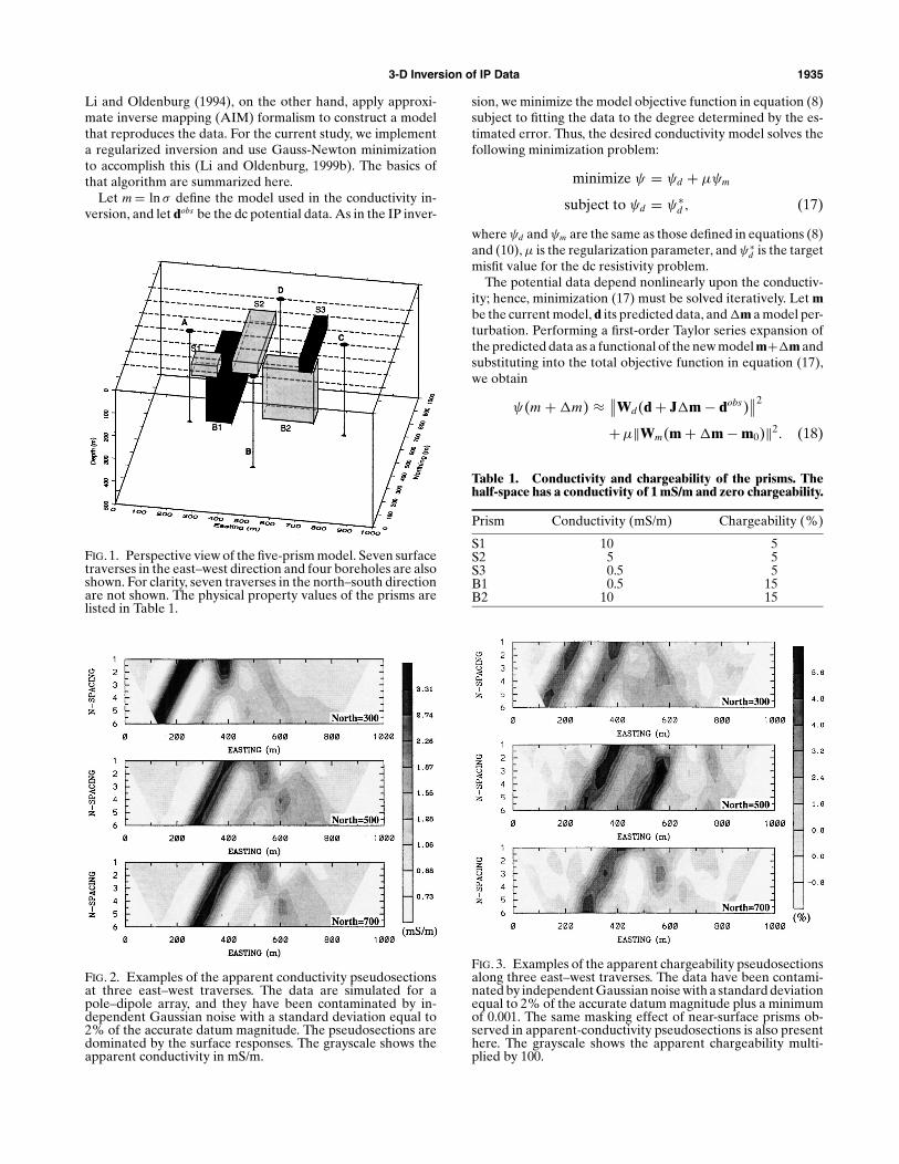
We now illustrate our algorithm using a test model com-posed of five anomalous rectangular prisms embedded in a uni-form half-space (Figure 1). Three surface prisms simulate near-surface distortions, and two buried prisms simulate deeper tar-gets. The conductivity and chargeability of the prisms are listedin Table 1. The dc resistivity and IP data from both surface andcrosshole experiments have been computed.

The surface experiment is carried out using a pole–dipolearray with a= 50 m and n= 1 to 6. There are seven traversesspaced 100 m apart in both east–west and north–south direc-tions. There are 1384 observations, and these have been con-taminated with uncorrelated Gaussian noise whose standarddeviation is equal to 2% of the datum value. Figures 2 and 3show apparent conductivity pseudosections and apparentchargeability pseudosections at three selected east–west tra-verses. The pseudosections are dominated by the responses tothe near-surface prisms, and there are only subtle indicationsof the buried conductive prism.

We first inverted the dc resistivity data using a Gauss-Newtonapproach that constructs a minimum structure model using amodel objective function similar to that in equation (8) butapplied to the logarithmic conductivity as the model. We setthe coefficients to αs = 0.0001 and αx = αy = αz = 1 and used areference conductivity model of 1 mS/m. The recovered con-ductivity model is shown by two plan sections and one crosssection in Figure 4. It is a reasonably good representation ofthe true conductivity model. All three surface prisms and theburied conductive prism are clearly imaged, and there is indi-cation of a resistive prism at depth. This conductivity model isthen used to calculate the sensitivity for the subsequent IP in-version. The inverted chargeability model is shown in Figure 5in the same plan and cross-sections. The surface prisms areclearly imaged, and the chargeability at depth is concentratedat the location of the two buried targets. The separation of thesebodies is not clearly defined, but this decrease of anomaly def-inition with increasing depth is expected when surface dataare inverted. Overall, the model is a good representation ofthe true anomalous chargeability zone. The contrast betweenthe pseudosections shown in Figure 3 and the cross-section ofthe recovered model in Figure 5 illustrates the improvementgained by performing the 3-D inversion.

CONSTRUCTION OF APPROXIMATE CONDUCTIVITIES

As discussed in the preceding section, the inversion of IPdata requires a background conductivity model for calculatingthe sensitivity. IP inversion is therefore a two-stage process,and its success depends upon the availability of a conductivitymodel that is a reasonable approximation to the true conduc-tivity. The usual approach to generating such a conductivitymodel is to invert the dc resistivity data that accompany theIP data. Numerous papers have been published on 3-D dc re-sistivity inversions, and different approaches have been pro-posed. For example, Park and Van (1991), Ellis and Oldenburg(1994a), Sasaki (1994), Zhang et al. (1995), and LaBrecque andMorelli (1996) all perform linearized inversion to construct aconductivity model from the dc resistivity data, although de-tails of their algorithms and implementations may vary greatly.


Li and Oldenburg (1994), on the other hand, apply approxi-mate inverse mapping (AIM) formalism to construct a modelthat reproduces the data. For the current study, we implementa regularized inversion and use Gauss-Newton minimizationto accomplish this (Li and Oldenburg, 1999b). The basics ofthat algorithm are summarized here.

Let m= ln σ define the model used in the conductivity in-version, and let dobs be the dc potential data. As in the IP inver-

FIG. 1. Perspective view of the five-prism model. Seven surfacetraverses in the east–west direction and four boreholes are alsoshown. For clarity, seven traverses in the north–south directionare not shown. The physical property values of the prisms arelisted in Table 1.

FIG. 2. Examples of the apparent conductivity pseudosectionsat three east–west traverses. The data are simulated for apole–dipole array, and they have been contaminated by in-dependent Gaussian noise with a standard deviation equal to2% of the accurate datum magnitude. The pseudosections aredominated by the surface responses. The grayscale shows theapparent conductivity in mS/m.

sion, we minimize the model objective function in equation (8)subject to fitting the data to the degree determined by the es-timated error. Thus, the desired conductivity model solves thefollowing minimization problem:

minimize ψ = ψd + µψm

subject to ψd = ψ∗d , (17)

where ψd and ψm are the same as those defined in equations (8)and (10), µ is the regularization parameter, and ψ∗

d is the targetmisfit value for the dc resistivity problem.

The potential data depend nonlinearly upon the conductiv-ity; hence, minimization (17) must be solved iteratively. Let mbe the current model, d its predicted data, and �m a model per-turbation. Performing a first-order Taylor series expansion ofthe predicted data as a functional of the new model m+�m andsubstituting into the total objective function in equation (17),we obtain

ψ(m + �m) ≈ ∥∥Wd(d + J�m − dobs)∥∥2

+ µ‖Wm(m + �m − m0)‖2. (18)

Table 1. Conductivity and chargeability of the prisms. Thehalf-space has a conductivity of 1 mS/m and zero chargeability.

Prism Conductivity (mS/m) Chargeability (%)

S1 10 5S2 5 5S3 0.5 5B1 0.5 15B2 10 15

FIG. 3. Examples of the apparent chargeability pseudosectionsalong three east–west traverses. The data have been contami-nated by independent Gaussian noise with a standard deviationequal to 2% of the accurate datum magnitude plus a minimumof 0.001. The same masking effect of near-surface prisms ob-served in apparent-conductivity pseudosections is also presenthere. The grayscale shows the apparent chargeability multi-plied by 100.


The value J is the sensitivity matrix of the potential data. Itselements are given by

Ji j = ∂φi

∂ ln σ j(19)

and are evaluated at the current model. Differentiating withrespect to �m and setting the derivative to zero yields theequation for the model perturbation:

(JTWT

d WdJ + µWmWm)�m

= −JTWTd Wd(d − dobs) − µWT

mWm(m − m0). (20)

FIG. 4. The conductivity model recovered from inversion ofsurface data using a Gauss-Newton method. The model isshown in one cross-section and two plan sections. The posi-tions of the true prisms are indicated by the white lines.

This is the basic equation solved for a Gauss-Newton step.The new model is then formed by updating the current model:m ← m + �m. This process is repeated iteratively until theminimization converges and an optimal value of µ is found toproduce the desired data misfit in equation (17).

The nonlinear inversion of 3-D dc resistivity data providesthe best approximation to the actual conductivity distribution,but it is a costly undertaking. One may not always want toexpend that amount of computation, especially when the re-covery of the conductivity model is but an intermediate step to-ward the end goal of constructing a chargeability model. Moreimportantly, good IP inversion results are often obtained byusing less rigorous approximations to the conductivity. Our

FIG. 5. The chargeability model recovered from inversion ofsurface data. The conductivity from full 3-D dc inversion isused to calculate sensitivities. The positions of the true prismsare indicated by the white lines.


experience with 2-D inversions (Oldenburg and Li, 1994) hasshown that good first-order results concerning the chargeabilitydistribution can often be obtained by approximating the earthusing a homogeneous conductive half-space. This suggests thata reasonable recovery of a 3-D chargeability model might beachieved by using intermediate approximations between thetwo end members corresponding to a uniform half-space andthe conductivity model recovered from a full nonlinear 3-D dcinversion.

To explore this, we compare five options for generating aconductivity model to be used in the IP inversion. The firstfour require much less computation than does the full 3-D in-version:

1) A uniform half-space: This is the simplest approximation,and no inversion of dc data is involved. When invert-ing apparent chargeability data, the actual value of thehalf-space conductivity is arbitrary since the sensitivity isindependent of it. However, when the secondary poten-tials are inverted, the best fitting half-space from the dcresistivity data should be used.

2) One-pass approximate 3-D inversion: This conductivitymodel is obtained from a linear inversion of the dcdata assuming that the actual conductivity consists ofweak perturbations of a uniform half-space (e.g., Li andOldenburg, 1994; Mø/ller et al., 1996). Such a modelcaptures the gross features in the conductivity structureand demands the least amount of computation. We haveimplemented the approximate inversion in the spatialdomain, in which the model objective function in equa-tion (8) is minimized explicitly so that a minimum struc-ture model is obtained. This is identical to performing thefirst iteration of the Gauss-Newton inversion with boththe initial and reference model being equal to the chosenbackground, mb. The equation to be solved is(

JTWTd WdJ + µWmWm

)�m

= −JTWTd Wd(d − dobs), (21)

where d is the predicted data. The approximate conduc-tivity is given by m = mb + �m.

3) Composite 2-D inversions: When surface data along par-allel traverses are available, independent 2-D inversionscan be carried out along each line so that a 2-D model thatreproduces the observations is generated (Oldenburget al., 1993; Loke and Barker, 1996). The series of 2-Dmodels are then combined to form a 3-D representationof the true conductivity structure. Such a model shouldperform well when there are strong 2-D features in thedata.

4) Limited 3-D AIM updates: Using the one-pass 3-D inver-sion as an AIM, we can iteratively update the conductivitymodel by the AIM algorithm (Oldenburg and Ellis, 1991)

Table 2. List of the dc and IP misfit for different approximations to the background conductivity. The dc misfit is calculated betweenthe observed dc resistivity data and the predicted data obtained from 3-D forward modeling of the approximate conductivities. TheIP misfit is the value achieved by the IP inversion when an approximate conductivity is used to calculate the sensitivity.

Misfit Half-space One-pass 3-D approximation 2-D composite Limited AIM updates Nonlinear inversion

DC 2.96 × 106 6.44 × 104 1.22 × 105 6.96 × 103 1.35 × 103

IP 2184 1720 1637 1634 1510

such that a final model reproducing the 3-D observationsis constructed. The greatest misfit reduction is achievedwithin the first two or three iterations (Li and Oldenburg,1994). Thus, by performing only a limited number of AIMupdates, we can obtain a conductivity model for the IPinversion. Let F−1 denote the one-pass approximate in-version and m be the current model. The model pertur-bation is defined by the difference between models gen-erated by applying the approximate inverse mapping tothe observed and predicted data, respectively:

m ← m + F−1[dobs] − F−1[d], (22)

where d is the predicted data from the current model.The iteration starts with an initial model which can besupplied by m = F−1[dobs].

5) Full 3-D nonlinear inversion: We use the Gauss-Newtoninversion discussed at the beginning of this section. Thisapproach provides the best approximation to the conduc-tivity, but it is the most computationally intensive. Eachiteration requires calculation of the sensitivity and sev-eral additional forward modelings.

The relative merits of these five methods will probably de-pend upon the complexity of the actual conductivity distribu-tion. A general statement may therefore be difficult to make,but insight can be obtained from applications to specific datasets. We have applied these five methods to the inversion ofour synthetic test data set shown in Figures 2 and 3.

We first focus upon generating the approximate conductiv-ities. The composite 2-D conductivity was obtained by invert-ing the data from the seven east–west lines using a 2-D algo-rithm and stitching together the resulting 2-D conductivities toform a 3-D model. The one-pass approximate 3-D inversionwas carried out using a uniform background of 1 mS/m and amodel objective function with αs = 0.0001 and αx = αy = αz = 1;we chose an optimal regularization parameter by the L-curvecriterion (Hansen, 1992) to account for both the linearizationerror and the added random errors. The selected regularizationparameter, together with the objective function, also definedthe approximate inverse mapping. We performed two itera-tions of AIM updates to produce the AIM approximation ofthe conductivity. Last, we had the conductivity model from afull 3-D inversion (Figure 4). For comparison, we have listedin Table 2 the data misfit between the observed dc potentialdata and the predicted data obtained by applying 3-D forwardmodeling to each of the five approximate conductivity mod-els. A comparison of these models with the true conductivitymodel is shown in Figure 6. We selected the cross-section atnorthing = 475 m, which passes through four of the five prismsin the model. The four models from different inversions showdifferent levels of detail about the conductivity anomaly, andthey present a general progression toward better representa-tions of the true model. However, the improvement diminishes


as the approximation approaches the best model that is ob-tained from the full 3-D inversion. Although the inverted con-ductivity models are similar, there is a substantial differencebetween the true model and any one of these approximations.

Using these five approximations to calculate the sensitivities,we performed five different inversions of the IP data. Sincesome of the conductivity models are poorer approximations,the corresponding IP inversions are not expected to achievethe expected data misfit. Instead, we chose an optimal regular-ization parameter for each inversion according to a generalizedcross-validation criterion. The result is that different inversionsmisfit the observed IP data by different amounts (Table 2).The resulting chargeability models are compared with the truemodel in Figure 7. Each panel in that figure is the cross-sectionof the recovered chargeability model at northing 475 m. Allfive models recover the essential features of the true model,and they present a general trend of improvement as the ap-proximation to the background conductivity improves. How-ever, the improvement in the recovered chargeability model isnot proportional to the increased computational cost involvedin constructing a better conductivity approximation. Less rig-orous approximations of conductivity which require much lesscomputation have produced good representations of the truechargeability model.

FIG. 6. Comparison between the five approximate conductivity models with the true conductivity. All sections are atnorthing = 475 m, which passes through four of the five prisms. The positions of the true prisms are outlined by the white boxes. Asthe approximation improves, the inverted conductivity model is a better representation of the true model.

JOINT INVERSION OF SURFACE AND CROSSHOLE DATACrosshole data have been used to achieve higher resolution

image of the subsurface structure obtained from dc resistivityand IP experiments (e.g., Spies and Ellis, 1995; LaBrecque andMorelli, 1996). However, although crosshole data are sensitiveto the vertical variation of conductivity and chargeability, theyhave rather poor sensitivity to the lateral variation because thedata have limited spatial distribution and the array separationis restricted to a small range. Surface data, however, usuallyhave good areal coverage and therefore possess better resolv-ing power for determining lateral variations in the subsurfacestructure. Surface data can provide good complementary in-formation to the crosshole data if the targets are within thedepth of penetration of the surface arrays. Joint inversion ofthese two data sets was expected to improve the resolution ofthe recovered chargeability model.

We placed four vertical boreholes around the anomalous re-gion in the test model. The locations are shown in Figure 1. Wesimulated crosshole data from a pole–dipole tomographic ex-periment. Current sources were placed along the source holefrom 0 to 400 m depth at an interval of 25 m. For each currentlocation, potentials in another borehole (receiver hole) weremeasured with a 50-m dipole at an interval of 25 m betweenz= 0 and 400 m. Figure 8 illustrates the electrode configuration


between two holes. Only one borehole in any pair of boreholeswas used as the source hole, and the reverse configuration ofswitching the source and receiver holes was not used. This re-sulted in six independent pairs of source–receiver holes.

A total of 1530 observations were generated for both dc andIP experiments using this configuration. Because of the pres-ence of zero crossings in the measured total potentials, we usedthe secondary potential, instead of apparent chargeability, asthe IP data. The data were contaminated with independentGaussian noise. The standard deviation for dc potentials wasequal to 2% of each accurate datum; for secondary potentialsit was equal to 5% of each accurate datum plus a minimumof 0.1 mV. (All the potentials were normalized to unit currentstrength.) Figure 9 displays the crosshole dc data as the appar-ent conductivity between two pairs of boreholes. The verticalaxis of the plot indicates the position of the current electrode inthe source hole, and the horizontal axis indicates the midpointof the potential dipole in the receiver hole. The data plots areremarkably featureless, and identification of individual prismsin the true model is impossible. Figure 10 displays the secondarypotentials in the same two pairs of boreholes. Again, there isno distinct feature in the secondary potential plots. The lackof distinct features in the borehole data is a direct indicationof the data’s poor sensitivities to the lateral variations in theconductivity and chargeability distributions.

FIG. 7. Comparison of chargeability models recovered from the 3-D inversion of surface IP data using five different approximationsto the background conductivity. The process by which each conductivity approximation is obtained is shown in each panel. Thelower-right panel is the true chargeability model.

Next, we compared the chargeability models obtained frominverting the crosshole data alone with the model obtainedby jointly inverting the surface and crosshole data. For thisstudy, we inverted the dc resistivity data using the full nonlinearinversion so that the best conductivity approximation at ourdisposal was used for the sensitivity calculation. In both dc andIP inversions, we chose a model objective function by settingthe coefficients to αs = 0.0001 and αx = αy = αz = 1. A uniformhalf-space of 1 mS/m was used as the reference model for dcresistivity inversion, and a zero reference model was used forthe IP inversion. In the inversions, the known values of the errorstandard deviations were used, and the target misfit value wasset to the number of data points being inverted. All inversionsconverged to the expected misfit value.

Figure 11 shows the conductivity model obtained from in-verting the crosshole dc resistivity data, displayed in two plansections and one cross-section. This model is a crude represen-tation of the true conductivity. Only the large surface conduc-tor and the buried conductor are identified, and the recoveredanomaly amplitude is very low. We used this conductivity in theinversion of crosshole IP data and the recovered chargeabilitymodel (Figure 12). This model is a poor representation of thetrue chargeability. Anomalies are recovered near the surface,but they do not correspond to the locations of the true prisms.The two deep prisms are marginally identified. The vertical


FIG. 8. Crosshole electrode configuration for collecting tomo-graphic data. The current source A in hole B moves at an in-terval of 25 m from z = 0 m to z = 400 m. For each currentlocation, the potential electrodes M and N , separated by 50 m,measure the potential differences in hole D. The midpoint ofthe potential dipole moves at an interval of 25 m from z = 25 mto z = 375 m. For a given pair of holes, no data are collectedby interchanging the current and potential holes.

FIG. 9. The crosshole plot of apparent-conductivity data. The vertical axis is the location of the current source in the source hole,and the horizontal axis is the midpoint of the potential dipole in the receiver hole. The left panel is for data between holes C andA, and the right panel is for data between holes B and D, as shown in Figure 1.

FIG. 10. The crosshole plot of secondary potential data in the same format as the crosshole apparent conductivity plots in Figure 8.The potentials are normalized to unit current strength, and the grayscale indicates the value in millivolts.

extent is well imaged, as would be expected from boreholedata, but the orientations and horizontal boundaries of therecovered anomalies differ from those of the true model. Inaddition, there is excessive structure in the region immediatelysurrounding the boreholes. This is typical when crosshole dataare inverted unless special weighting in the objective functionis included to counter it.

We next jointly inverted the surface data in Figures 2 and 3and the crosshole data in Figures 8 and 9. Figure 13 displaysthe recovered conductivity model from the joint inversion ofsurface and borehole data. This model is dominated by the fea-tures recovered in the surface data inversion. The minor im-provements are the increased amplitude and the slightly betterdefinition of the depth extent of the conductivity prism. Usingthis model we calculated the sensitivity and then performed thejoint inversion of the two IP data sets to recover the chargeabil-ity model shown in Figure 14. It shows dramatic improvementcompared with the models from individual inversions in Fig-ures 5 and 12. All five prisms are well resolved, and artifactssurrounding the boreholes are minimized. The most noticeableimprovement is the clear image of the two separate buried tar-gets. The recovered amplitudes, positions, and orientations ofthe two anomalies all correspond well with the true model.


FIELD EXAMPLE

As our last example, we illustrate the 3-D inversion algo-rithm using a set of pole–dipole data from the Mt. Milligancopper–gold porphyry deposit in central British Columbia,Canada. These data were first analyzed by Oldenburg et al.(1997) using a 2-D algorithm. We invert them using the 3-Dalgorithm, which illustrates the 3-D inversion in a mineral ex-ploration setting and provides a comparison with the resultfrom a series of 2-D inversions.

The Mt. Milligan deposit lies within the Early MesozoicQuesnel terrane, which hosts a number of Cu-Au porphyry de-posits, and it occurs within porphyritic monzonite stocks andadjacent volcanic rocks. The initial deposit model consists of avertical monzonitic stock, known as the MBX stock, intruded

FIG. 11. Conductivity model recovered from the crosshole dataalone. This model shows an elongated conductor on the sur-face and a broad conductor at depth. Both conductors are sur-rounded by resistive halos, and the amplitude is small.

into volcanic host rocks. Dykes extend from the stock andcut through the porous trachytic units in the host. Emplace-ment of the monzonite intrusive is accompanied by intensivehydrothermal alteration primarily near the boundaries of thestock and in and around the porous trachytic units cross-cutby monzonite dykes. Potassic alteration, which produced chal-copyrite, occurs in a region surrounding the initial stock, and itsintensity decreases away from the boundary. Propylitic alter-ation, which produces pyrite, exists outward from the potassicalteration zone. Strong IP effects are produced by these alter-ation products, and the IP survey is well suited for mappingthe alteration zones. The pole–dipole dc resistivity and IP sur-veys over Mt. Milligan were carried out along east–west linesspaced 100 m apart. The dipole length was 50 m, and n-spacingwas from 1 to 4. This yielded 946 data points along 11 lines in

FIG. 12. Chargeability model recovered from the crossholedata alone. This model shows little resolution near the sur-face where the anomalies are confined to small volumes. Thedeeper anomalies are identified but not well resolved. As ex-pected, the depth extent of the buried chargeable bodies is welldelineated.


our study area of 1.2 × 1.0 km. This area, directly above theMBX stoc, has a gentle surface topography, and the total reliefis about 100 m. Figure 15 displays the apparent chargeabilitydata in plan maps of constant n-spacings. For brevity, we havenot shown the dc resistivity data here. The apparent chargeabil-ity data show large anomalies toward the western and southernregions. The north-central region of low apparent chargeabilityis related to the intrusive stock that has significantly less sulfidefrom the alteration processes.

To invert these data, we used a mesh that consisted of cells25 m wide in both horizontal directions and 12.5 m thick inthe region of interest. The mesh was extended horizontally anddownward by cells of increasing sizes. The total number of cellsin the inversion was about 72 000. We first performed the fullnonlinear inversion of the DC resistivity data and then used it to

FIG. 13. Conductivity model recovered from the joint inversionof surface and crosshole data. This model is similar to thatobtained from surface data alone, but it has a slightly higheramplitude for the buried conductive anomaly. The depth extentof the anomaly is also slightly better defined.

carry out the IP inversion. The resulting model is shown in Fig-ure 16. For comparison, we also plotted the chargeability modelcreated by combining the 2-D sections obtained from invertingthe 11 lines of data separately using a 2-D algorithm. The re-covered 3-D chargeability models from these two approacheswere consistent, and they both imaged the large-scale anoma-lies reasonably well. This was not surprising since the limitedarray length meant there was little redundant information inthe data from adjacent lines. The model recovered from the 3-D inversion was somewhat smoother and showed less spuriousstructure than the composite 2-D model. It also showed a well-defined central zone of low chargeability at depth. This was aclearer image of the monzonite stock than what was imaged inthe 2-D inversions.

FIG. 14. Chargeability model recovered from the joint inver-sion of surface and crosshole data. This model shows the greatimprovement achieved by joint inversion of the two comple-mentary data sets. All five anomalies are well resolved. Es-pecially noticeable is that the boundaries of the two buriedchargeable bodies are well delineated.


DISCUSSION

We developed a 3-D IP inversion algorithm that applies todata acquired using arbitrary electrode configurations on a to-pographically variable earth surface or in boreholes. We as-sumed that the chargeability is small and formulated the in-version as a two-step process. First, the dc resistivity data areinverted to generate a background conductivity. That conduc-tivity is used to generate the sensitivity matrix for the IP equa-tions. The 3-D chargeability model is then generated by solvingthe system of equations, subject to a restriction that the charge-ability is everywhere positive and smaller than an upper bound.

The analysis of large IP data sets often takes place in stages.The first goal is to obtain an image that reveals the major sub-surface structures, answers questions about the existence ofburied targets, and supplies approximate details about size andlocation. Major components affecting this image are the choiceof model objective function, the amount and type of errors onthe data, and the degree to which the data are fit. For our two-step process, we must also pay attention to how valid the lin-earization process is and how close the recovered conductivityis to the true conductivity.

The question of how close the recovered conductivity needsto be to the true conductivity so that sensitivity J is a good esti-mate of the true sensitivities is not addressed quantitatively inthis paper. We have, however, carried out an empirical test ina single example. Four approximate conductivities were usedto generate the sensitivities. In general, higher quality dc in-

FIG. 15. The IP data from an area above the MBX stock of the Mt. Milligan copper–gold porphyry deposit in central BritishColumbia. The data were acquired using a pole–dipole array with a dipole length of 50 m and n-spacing from 1 to 4. The four panelsare plan maps of the data corresponding to different n-spacings.

versions yielded better IP results, with the half-space conduc-tivity, a one-pass linearized inversion, a few passes of an AIMapproach, and the Gauss-Newton inversion giving progressiveimprovement. However, the differences in the final IP inver-sions from these various approximations were fairly subtle (seeFigure 7). In fact, these differences were smaller than changesin the image obtained by adjusting the degree to which the dataare misfit or by slightly altering the model objective functionbeing minimized. Yet the various approximations to the con-ductivity can be produced with substantially fewer computa-tions than the full Gauss-Newton solution. This allows the userto carry out a number of first-pass inversions with a data setto achieve insight about the gross distribution of earth charge-ability. If the conductivity structure is not overly complicated,then this result may be satisfactory for final interpretation. Thequestion of how well the conductivity must be known is a po-tential area for further research.

Another approximate conductivity model is that generatedby combining results from 2-D inversions. The prevalence of2-D inversion algorithms means that this information is gen-erally available when data have been collected along parallellines. We know that off-line anomalies and 3-D topography willcause distortions in the recovered 2-D conductivity models, sosome degree of caution is required. In the synthetic modelingpresented here and in the Mt. Milligan example, the 2-D anal-ysis for conductivity worked satisfactorily. Further research isrequired to provide more detailed rules about when 2-D is ap-plicable.


An important aspect of our IP inversion is the incorporationof upper and lower bounds on the chargeability. The lowerbound is physical since chargeability is positive. The upperbound might be (1) assignable from a priori knowledge aboutthe nature of the mineralization or (2) assigned to generate amodel consistent with the linearized formulation of the equa-tions. Linearization requires that the chargeability be small.The positivity and upper bounds are implemented through aprimal logarithmic barrier method. This increases the complex-ity of the algorithm, but the method is well established in theliterature and we provide an explicit algorithm for its imple-mentation.

Another major component of our algorithm is the introduc-tion of the wavelet transform to perform the matrix–vectormultiplications. The sensitivity matrix can be compressed by afactor of at least 10. This leads to substantial savings in both re-

FIG. 16. Comparison of the chargeability models obtained from 2-D and 3-D inversions of the data from Mt. Milligan shown inFigure 15. The column on the left shows one cross-section and two plan sections of the 3-D model obtained by combining eleven 2-Dsections recovered from 2-D inversions. The column on the right shows the model obtained by performing a single 3-D inversionof all the data. The two results are generally consistent. However, less spurious structure is present in the model from the 3-Dinversion, and the central zone of low chargeability corresponding to the MBX stock is imaged better.

quired memory and CPU time. This has made the algorithm atleast ten times faster than a direct approach and consequentlyhas allowed us to routinely handle problems that have a fewthousand data and a hundred thousand cells with relative effi-ciency.

Last, the application of our algorithm to joint surface andcrosshole data has demonstrated that the inversion of these twocomplementary data sets can greatly improve the resolutionof the inverted chargeability model. The noticeable gains arein the enhanced definition of both horizontal boundary andvertical extent of buried chargeable zones.

ACKNOWLEDGMENTS

We thank Roman Shekhtman for his valuable assistancein programming the code and in running numerical exam-ples. This work has been supported by an NSERC IOR grant


and an industry consortium, 3-D Inversion of DC resistivityand Induced Polarization Data (INDI). Participating compa-nies are Placer Dome, BHP Minerals, Cominco Exploration,Falconbridge, INCO Exploration & Technical Services, New-mont Gold Company, and Rio Tinto Exploration.

REFERENCES

Dey, A., and Morrison, H. F., 1979, Resistivity modelling for arbitrarilyshaped three-dimensional structures: Geophysics, 44, 753–780.

Ellis, R. G., and Oldenburg, D. W., 1994a, The pole-pole 3-D DC-resistivity inverse problem: A conjugate-gradient approach: Geo-phys. J. Internat., 119, 187–194.

——— 1994b, 3-D induced polarization inversion using conjugate gra-dients: Presented at the John Sumner Memorial Internat. Workshopon Induced Polarization (IP) in Mining and the Environment.

Gill, P. E., Murray, W., Ponceleon, D. B., and Saunders, M., 1991, Solvingreduced KKT systems in barrier methods for linear and quadraticprogramming: Stanford Univ. Technical Report SOL 91–7.

Golub, G. H., Heath, M., and Wahba, G., 1979, Generalized cross-validation as a method for choosing a good ridge parameter: Tech-nometrics, 21, 215–223.

Haber, E., and Oldenburg, D. W., 2000, A GCV-based method fornonlinear ill-posed problems: Comp. Geosci., in press.

Hansen, P. C., 1992, Analysis of discrete ill-posed problems by meansof the L-curve: SIAM Review, 34, 561–580.

Kowalczyk, P. L., Logan, K. J., and Bradshaw, P. M. D., 1997, Newmethods in geophysics to visualize geology in tropical terrains: 4thDecennial Internat. Conf. Min. Expl., Proceedings, 829–834.

LaBrecque, D. J., 1991, IP tomography: 61st Ann. Internat. Mtg., Soc.Expl. Geophys., Expanded Abstracts, 413–416.

LaBrecque, D. J., and Morelli, G., 1996, 3-D electrical resistivity to-mography for environmental monitoring: Symp. on Appl. Geophys.to Engin. and Environ. Problems, Proceedings.

Li, Y., and Oldenburg, D. W., 1994, Inversion of 3-D DC resistivity datausing an approximate inverse mapping: Geophys. J. Internat., 116,527–537.

——— 1999a, Fast inversion of large scale magnetic data using wavelettransforms: Geophysical J. Internat., accepted for publication.

——— 1999b, 3-D inversion of DC resistivity data using an L-curvecriterion: 69th Ann. Internat. Mtg., Soc. Expl. Geophys., Expanded

Abstracts, 251–254.Loke, M. H., and Barker, R. D., 1996, Rapid least-squares inversion of

apparent conductivity pseudosection using a quasi-Newton method:Geophys. Prosp., 44, 131–152.

McGillivary, P. R., and Oldenburg, D. W., 1990, Methods for calculatingFrechet derivatives and sensitivities for nonlinear inverse problem:A comparative study: Geophys. Prosp., 38, 499–524.

Møller, I., Christensen, N. B., and Jacobsen, B. H., 1996, 2-D inversionof resistivity profile data: Symp. on Appli. Geophys. to Engin. andEnviron. Problems, Proceedings.

Mutton, A. J., 1997, The application of geophysics during evaluation ofthe Century zinc deposit: 4th Decennial Internat. Conf. Min. Expl.,Proceedings, 599–614.

Oldenburg, D. W., and Ellis, R. G., 1991, Inversion of geophysical datausing an approximate inverse mapping: Geophys. J. Internat., 105,325–353.

Oldenburg, D. W., and Li, Y., 1994, Inversion of induced polarizationdata: Geophysics, 59, 1327–1341.

Oldenburg, D. W., McGillivary, P. R., and Ellis, R. G., 1993, General-ized subspace method for large scale inverse problems: Geophys. J.Internat., 114, 12–20.

Oldenburg, D. W., Li, Y., and Ellis, R. G., 1997, Inversion of geophys-ical data over a copper-gold porphyry deposit: A case history forMt. Milligan: Geophysics, 62, 1419–1431.

Park, S. K., and Van, G. P., 1991, Inversion of pole-pole data for 3-Dresistivity structure beneath arrays of electrodes: Geophysics, 56,951–960.

Sasaki, Y., 1994, 3-D resistivity inversion using the finite-elementmethod: Geophysics, 59, 1839–1848.

Saunders, M., 1995, Cholesky-based methods for sparse least squares:The benefits of regularization: Stanford Univ. Technical Report SOL95–1.

Seigel, H. O., 1959, Mathematical formulation and type curves for in-duced polarization: Geophysics, 24, 547–565.

Spies, B. R., and Ellis, R. G., 1995, Cross-borehole resistivity tomogra-phy of a pilot-scale, in-situ vitrification test: Geophysics, 60, 886–898.

Tikhonov, A. V., and Arsenin, V. Y., 1977, Solution of ill-posed prob-lems, ed. J. Fritz: John Wiley & Sons.

Wahba, G., 1990, Spline models for observational data: Soc. Ind. Appl.Math.

Zhang, J., MacKie, R. D., and Madden, T. R., 1995, 3-D resistivityforward modelling and inversion using conjugate gradients: Geo-physics, 60, 1313–1325.

Paper GEM

Documents

d ip data

ip inversions

dc resistivity data

pass3d inversions

d nonlinear inversions

apparent chargeability

d earthstructure

d environment