2012 EDITION | Study System ® ATC International became a part of Becker Professional Education in 2011. ATC International has 20 years of experience providing lectures and learning tools for ACCA Professional Qualifications. Together, Becker Professional Education and ATC International offer ACCA candidates high quality study materials to maximize their chances of success. ACCA Paper F5 | PERFORMANCE MANAGEMENT

Welcome message from author
This document is posted to help you gain knowledge. Please leave a comment to let me know what you think about it! Share it to your friends and learn new things together.
Transcript

2012 EDITION | Study System
®
®
ATC International became a part of Becker
Professional Education in 2011. ATC International
has 20 years of experience providing lectures
and learning tools for ACCA Professional
Qualifications. Together, Becker Professional
Education and ATC International offer ACCA
candidates high quality study materials to maximize
their chances of success.
ACCA Paper F5 | PERFORMANCE MANAGEMENT

In 2011 Becker Professional Education, a global leader in professional education, acquired ATC
International. ATC International has been developing study materials for ACCA for 20 years, and
thousands of candidates studying for the ACCA Qualification have succeeded in their professional
examinations through its Platinum and Gold ALP training centers in Central and Eastern Europe and
Central Asia.*
Becker Professional Education-ATC International has also been awarded ACCA Approved Learning
Partner-content Gold Status for materials for the Diploma in International Financial Reporting (DipIFR).
Nearly half a million professionals have advanced their careers through Becker Professional Education's
courses. Throughout its more than 50 year history, Becker has earned a strong track record of student
success through world-class teaching, curriculum and learning tools.
Together with ATC International, we provide a single destination for individuals and companies in need of
global accounting certifications and continuing professional education.
*Platinum – Moscow, Russia and Kiev, Ukraine. Gold – Almaty, Kazakhstan
BECKER PROFESSIONAL EDUCATION’S ACCA STUDY MATERIALS
All of Becker’s materials are authored by experienced ACCA lecturers and are used in the delivery of
classroom courses.
Study System*: Provides comprehensive coverage of the core syllabus areas and is designed to be
used both as a reference text and as part of integrated study to provide you with the knowledge, skill and
confidence to succeed in your ACCA examinations. It also includes a bank of practice questions relating
to each topic covered.
Revision Question Bank*: Exam style and standard questions with model answers to give guidance in
final preparation.
Revision Essentials: A condensed, easy-to-use aid to revision containing essential technical content,
examiners' insights and exam guidance.
* ACCA Gold Approved Learning Partner – content
®
LICENSE AGREEMENT DO NOT USE ANY OF THESE MATERIALS UNTIL YOU HAVE READ THIS AGREEMENT CAREFULLY. IF YOU USE ANY OF THE MATERIALS, YOU ARE AGREEING AND CONSENTING TO BE BOUND BY AND ARE BECOMING A PARTY TO THIS AGREEMENT. These materials are NOT for sale and are not being sold to you. You may NOT transfer these materials to any other person or permit any other person to use these materials. You may only acquire a license to use these materials and only upon the terms and conditions set forth in this license agreement. Read this agreement carefully before using these materials. Do not use these materials unless you agree with all terms of this agreement. NOTE: You may already be a party to this agreement if you are registered for a Becker Professional Education® ACCA course. (the "Course"), or if you placed an order for these materials on-line or using a printed form that included this license agreement. Please review the termination section regarding your rights to terminate this license agreement and receive a refund of your payment. Grant: Upon your acceptance of the terms of this agreement, in a manner set forth above, DeVry/Becker Educational Development Corp. ("Becker") hereby grants to you a non-exclusive, revocable, non-transferable, non-sublicensable, limited license to use the materials, including eBooks ("Materials"), as defined below, and any Materials to which you are granted access as a result of your license to use the Materials and/or in connection with the Course on the following terms: You may: • use the Materials for the Course, for preparation for one or more parts of the ACCA exam (the "Exam"), and/or for your studies relating to the
subject matter covered by the Course and/or the Exam; and • take electronic and/or handwritten notes during the Program; provided, however, that all notes taken by you during the Course that relate to the
subject matter of the Course are and shall remain Materials subject to the terms of this agreement. You may not: • use the Materials for any purpose other than as expressly permitted above; • make copies of all or any part of the Materials; • rent, lease, license, lend, or otherwise transfer or provide (by gift, sale, or otherwise) all or any part of the Materials to anyone; • permit the use of all or any part of the Materials by anyone other than you; or • create derivative works of the Materials. Materials: Materials means and includes any and all written and electronic materials provided to you in connection with the Course and/or otherwise provided to you and/or to which you are otherwise granted access by Becker (directly or indirectly) in connection with your license of the accompanying materials and/or the Course, and shall include notes you take (by hand, electronically, digitally, or otherwise) during the Course relating to the subject matter of the Course. Materials may include, but are not limited to, one or more hardcover workbooks and/or eBooks (books in electronic format) for each of the subject matter areas of the Exam. Title: Becker is and will remain the owner of all title, ownership rights, intellectual property, and all other rights and interests in and to the Materials and all other Materials that are subject to the terms of this agreement. The Materials are protected by the copyright laws of the United States and international copyright laws and treaties. Termination: This license shall terminate the earlier of: (i) ten (10) business days after notice to you of non-payment of or default on any payment due Becker which has not been cured within such 10 day period; or (ii) immediately if you fail to comply with any of the limitations described above. On termination of this license in its entirety, you must destroy all copies of the Materials, including, but not limited to, any archival copies you may have made. On termination of this license with respect to a particular Material, you must destroy such Material, including, but not limited to, any archival copies you may have made. Your Limited Right to Terminate this License and Receive a Refund: You may terminate this license in accordance with Becker's refund policy as provided at www.beckeratci.com No Warranty: BECKER MAKES NO WARRANTIES, EXPRESS OR IMPLIED, WITH RESPECT TO THE PRINTED MATERIALS, THEIR MERCHANTABILITY OR FITNESS FOR A PARTICULAR PURPOSE AND NO WARRANTY OF NONINFRINGEMENT OF THIRD PARTIES' RIGHTS. NO DEALER, AGENT OR EMPLOYEE OF BECKER IS AUTHORIZED TO MAKE ANY MODIFICATIONS, EXTENSIONS OR ADDITIONS TO THIS NO WARRANTY. Exclusion of Damages: UNDER NO CIRCUMSTANCES AND UNDER NO LEGAL THEORY, TORT, CONTRACT, OR OTHERWISE, SHALL BECKER OR ITS DIRECTORS, OFFICERS, EMPLOYEES OR AGENTS, BE LIABLE TO YOU OR ANY OTHER PERSON FOR ANY CONSEQUENTIAL, INCIDENTAL, INDIRECT, PUNITIVE, EXEMPLARY OR SPECIAL DAMAGES OF ANY CHARACTER, INCLUDING, WITHOUT LIMITATION, DAMAGES FOR LOSS OF GOODWILL, WORK STOPPAGE, COMPUTER FAILURE OR MALFUNCTION OR ANY AND ALL OTHER DAMAGES OR LOSSES, OR FOR ANY DAMAGES IN EXCESS OF BECKER'S LIST PRICE FOR A LICENSE TO THE MATERIALS, EVEN IF BECKER SHALL HAVE BEEN INFORMED OF THE POSSIBILITY OF SUCH DAMAGES, OR FOR ANY CLAIM BY ANY OTHER PARTY. Indemnification and Remedies: You agree to indemnify and hold Becker and its employees, representatives, agents, attorneys, affiliates, directors, officers, members, managers and shareholders harmless from and against any and all claims, demands, losses, damages, penalties, costs or expenses (including reasonable attorneys' and expert witness' fees and costs) of any kind or nature, arising from or relating to any violation, breach or nonfulfillment by you of any provision of this license. If you are obligated to provide indemnification pursuant to this provision, Becker may, in its sole and absolute discretion, control the disposition of any indemnified action at your sole cost and expense. Without limiting the foregoing, you may not settle, compromise or in any other manner dispose of any indemnified action without the consent of Becker. If you breach any material term of this license, Becker shall be entitled to equitable relief by way of temporary and permanent injunction and such other and further relief as any court with jurisdiction may deem just and proper. Severability of Terms: If any term or provision of this license is held invalid or unenforceable by a court of competent jurisdiction, such invalidity shall not affect the validity or operation of any other term or provision and such invalid term or provision shall be deemed to be severed from the license. This license agreement may only be modified by written agreement signed by both parties. Governing Law: This license agreement shall be governed and construed according to the laws of the state of Illinois, save for any choice of law provisions. Any legal action regarding this Agreement shall be brought only in the U.S. District Court for the Northern District of Illinois, or another court of competent jurisdiction in DuPage County, Illinois, and all parties hereto consent to jurisdiction and venue in DuPage County, Illinois. ACCA and Chartered Certified Accountants are registered trademarks of The Association of Chartered Certified Accountants and may not be used without their express, written permission. Becker Professional Education is a registered trademark of DeVry/Becker Educational Development Corp. and may not be used without its express, written permission.

©2012 DeVry/Becker Educational Development Corp. All rights reserved.
ACCA
PAPER F5
PERFORMANCE MANAGEMENT
STUDY SYSTEM
JUNE 2012
®
©2012 DeVry/Becker Educational Development Corp. All rights reserved.
No responsibility for loss occasioned to any person acting or refraining from action as a result of any material in this publication can be accepted by the author, editor or publisher.
This training material has been published and prepared by Accountancy Tuition Centre (International Holdings) Limited
16 Elmtree Road Teddington TW11 8ST United Kingdom.
Copyright ©2012 DeVry/Becker Educational Development Corp. All rights reserved.
No part of this training material may be translated, reprinted or reproduced or utilised in any form either in whole or in part or by any electronic, mechanical or other means, now known or hereafter invented, including photocopying and recording, or in any information storage and retrieval system. Request for permission or further information should be addressed to the Permissions Department, DeVry/Becker Educational Development Corp.
.
SESSION 00 – CONTENTS
©2012 DeVry/Becker Educational Development Corp. All rights reserved. (iii)
CONTENTS
Page
Introduction (v)
Syllabus (vi)
Study Guide (x)
Formulae (xv)
Exam technique (xvi)
1 Traditional management and cost accounting 0101
2 Activity based costing 0201
3 Developments in management accounting 0301
4 Relevant cost analysis 0401
5 Cost Volume Analysis 0501
6 Limiting factor decisions 0601
7 Pricing 0701
8 Risk and uncertainty 0801
9 Budgeting 0901
10 Quantitative Techniques for Budgeting 1001
11 Budgeting and standard costing 1101
12 Basic variance analysis 1201
13 Advanced variance analysis 1301
14 Behavioural aspects of standard costing 1401
15 Performance measurement 1501
16 Further aspects of performance measurement 1601
17 Divisional performance evaluation 1701
18 Transfer pricing 1801
Index 1901

SESSION 00 – CONTENTS
(iv) ©2012 DeVry/Becker Educational Development Corp. All rights reserved.
SESSION 00 – INTRODUCTION
©2012 DeVry/Becker Educational Development Corp. All rights reserved. (v)
Introduction
This Study System has been specifically written for the Association of Chartered Certified Accountants fundamentals level examination, Paper F5 Performance Management.
It provides comprehensive coverage of the core syllabus areas and is designed to be used both as a reference text and interactively with the ATC Learning System to provide you with the knowledge, skill and confidence to succeed in your ACCA studies.
About the author: Nick Ryan is ATC International’s lead tutor in performance management and has more than 10 years’ experience in delivering ACCA exam-based training.
How to use this Study System
You should first read through the syllabus, study guide and approach to examining the syllabus provided in this session to familiarise you with the content of this paper. The sessions which follow include:
An overview diagram at the beginning of each session. This provides a visual summary of the topics covered in each Session and how they are related
The body of knowledge which underpins the syllabus. Features of the text include:
Definitions Terms are defined as they are introduced.
Illustrations These are to be read as part of the text. Any solutions
to numerical illustrations follow on immediately.
Examples These should be attempted using the proforma solution provided (where applicable).
Key points Attention is drawn to fundamental rules and
underlying concepts and principles.
Commentaries These provide additional information.
Focus These are the learning outcomes relevant to the
session, as published in ACCA’s Study Guide.
Example solutions are presented at the end of each session.
A bank of practice questions is contained in the Study Question Bank provided. These are linked to the topics of each session and should be attempted after studying each session.

SESSION 00 – SYLLABUS
(vi) ©2012 DeVry/Becker Educational Development Corp. All rights reserved.
SYLLABUS
Aim
To develop knowledge and skills in the application of management accounting techniques to quantitative and qualitative information for planning, decision-making, performance evaluation, and control
Main capabilities
On successful completion of this paper candidates should be able to:
A Explain, apply, and evaluate cost accounting techniques.
B Select and appropriately apply decision-making techniques to evaluate business choices and promote efficient and effective use of scarce business resources, appreciating the risks and uncertainty inherent in business and controlling those risks.
C Apply budgeting techniques and evaluate alternative methods of budgeting, planning and control.
D Use standard costing systems to measure and control business performance and to identify remedial action.
E Assess the performance of a business from both a financial and non-financial viewpoint, appreciating the problems of controlling divisionalised businesses and the importance of allowing for external aspects.
Rationale
The syllabus for Paper F5, Performance Management, builds on the knowledge gained in Paper F2, Management Accounting. It also prepares candidates for more specialist capabilities which are covered in P5 Advanced Performance Management.
The syllabus begins by introducing more specialised management accounting topics. There is some knowledge assumed from Paper F2 – primarily overhead treatments. The objective here is to ensure candidates have a broader background in management accounting techniques.
The syllabus then considers decision-making. Candidates need to appreciate the problems surrounding scarce resource, pricing and make-or-buy decisions, and how this relates to the assessment of performance. Risk and uncertainty are a factor of real-life decisions and candidates need to understand risk and be able to apply some basic methods to help resolve the risks inherent in decision-making.
Budgeting is an important aspect of many accountants’ lives. The syllabus explores different budgeting techniques and the problems inherent in them. The behavioural aspects of budgeting are important for accountants to understand, and the syllabus includes consideration of the way individuals react to a budget.

SESSION 00 – SYLLABUS
©2012 DeVry/Becker Educational Development Corp. All rights reserved. (vii)
Standard costing and variances are then built on. All the variances examined in Paper F2 are examinable here. The new topics are mix and yield variances, and planning and operational variances. Again, the link is made to performance management. It is important for accountants to be able to interpret the numbers that they calculate and ask what they mean in the context of performance.
The syllabus concludes with performance measurement and control. This is a major area of the syllabus. Accountants need to understand how a business should be managed and controlled. They should appreciate the importance of both financial and non-financial performance measures in management. Accountants should also appreciate the difficulties in assessing performance in divisionalised businesses and the problems caused by failing to consider external influences on performance. This section leads directly to Paper P5.
Relational diagram of main capabilities
Specialist cost and management accounting
techniques (A)
Decision-making techniques (B)
Budgeting (C)
Standard costing and variance analysis (D)
Performance measurement and
control (E)
Syllabus structure
APM (P5)
PM (F5)
MA (F2)

SESSION 00 – SYLLABUS
(viii) ©2012 DeVry/Becker Educational Development Corp. All rights reserved.
Detailed syllabus
A Specialist cost and management accounting techniques
1. Activity-based costing
2. Target costing
3. Life-cycle costing
4. Throughput accounting
5. Environmental Accounting
B Decision-making techniques
1. Relevant cost analysis
2. Cost volume profit analysis
3. Limiting factors
4. Pricing decisions
5. Make or buy and other short term decisions
6. Dealing with risk and uncertainty in decision-making
C Budgeting
1. Objectives
2. Budgetary systems
3. Types of budget
4. Quantitative analysis in budgeting
5. Behavioural aspects of budgeting
D Standard costing and variances analysis
1. Budgeting and standard costing
2. Basic variances and operating statements
3. Material mix and yield variances
4. Sales mix and quantity variances
5. Planning and operational variances
6. Behavioural aspects of standard costing
E Performance measurement and control
1. The scope of performance measurement
2. Divisional performance and transfer pricing
3. Performance analysis in not-for-profit organisations and the public sector
4. External considerations and behavioural aspects
SESSION 00 – SYLLABUS
©2012 DeVry/Becker Educational Development Corp. All rights reserved. (ix)
Approach to examining the syllabus
Paper F5, Performance Management, seeks to examine candidates’ understanding of how to manage the performance of a business.
The paper builds on the knowledge acquired in Paper F2, Management Accounting, and prepares those candidates who choose to study Paper P5, Advanced Performance Management, at the Professional level.
The syllabus is assessed by a three-hour paper-based examination. The examination contains five compulsory 20-mark questions. There will be calculation and discursive elements to the paper with the balance being broadly in line with the pilot paper. The pilot paper contains questions from four of the five syllabus sections. Generally, the paper will seek to draw questions from as many of the syllabus sections as possible.
ACCA Support
For examiner’s reports, guidance and technical articles relevant to this paper see http://www2.accaglobal.com/students/acca/exams/f5/
The ACCA’s Study Guide which follows is referenced to the Sessions in this Study System.
SESSION 00 – STUDY GUIDE
(x) ©2012 DeVry/Becker Educational Development Corp. All rights reserved.
STUDY GUIDE
A SPECIALIST COST AND MANAGEMENT ACCOUNTING TECHNIQUES
1. Activity based costing
Identify appropriate cost drivers under ABC.
Calculate costs per driver and per unit using ABC.
Compare ABC and traditional methods of overhead absorption based on production units, labour hours or machine hours.
2. Target costing
Derive a target cost in manufacturing and service industries.
Explain the difficulties of using target costing in service industries.
Suggest how a target cost gap might be closed.
3. Life-cycle costing
Identify the costs involved at different stages of the life-cycle.
Derive a life cycle cost in manufacturing and service industries.
Identify the benefits of life cycle costing.
4. Throughput accounting
Calculate and interpret a throughput accounting ratio (TPAR).
Suggest how a TPAR could be improved.
Apply throughput accounting to a multi-product decision-making problem.
Ref: 2 3 3 3
5. Environmental accounting
Discuss the issues business face in the management of environmental costs.
Describe the different methods a business may use to account for its environmental costs.
B DECISION-MAKING TECHNIQUES
1. Relevant cost analysis
Explain the concept of relevant costing.
Identify and calculate relevant costs for a specific decision situations from given data.
Explain and apply the concept of opportunity costs.
2. Cost volume profit analysis
Explain the nature of CVP analysis.
Calculate and interpret breakeven point and margin of safety.
Calculate the contribution to sales ratio, in single and multi-product situations, and demonstrate an understanding of its use.
Calculate target profit or revenue in single and multi-product situations, and demonstrate an understanding of its use.
Prepare break even charts and profit volume charts and interpret the information contained within each, including multi-product situations.
Discuss the limitations of CVP analysis for planning and decision making.
Ref: 3 4 5

SESSION 00 – STUDY GUIDE
©2012 DeVry/Becker Educational Development Corp. All rights reserved. (xi)
3. Limiting factors
Identify limiting factors in a scarce resource situation and select an appropriate technique.
Determine the optimal production plan where an organisation is restricted by a single limiting factor, including within the context of “make” or “buy” decisions.
Formulate and solve multiple scarce resource problem both graphically and using simultaneous equations as appropriate.
Explain and calculate shadow prices (dual prices) and discuss their implications on decision-making and performance management.
Calculate slack and explain the implications of the existence of slack for decision-making and performance management. (Excluding simplex and sensitivity to changes in objective functions)
4. Pricing decisions
Explain the factors that influence the pricing of a product or service.
Explain the price elasticity of demand.
Derive and manipulate a straight line demand equation. Derive an equation for the total cost function (including volume-based discounts).
Calculate the optimum selling price and quantity for an organisation, equating marginal cost and marginal revenue
Evaluate a decision to increase production and sales levels, considering incremental costs, incremental revenues and other factors.
Ref: 6 7
Determine prices and output levels for profit maximisation using the demand based approach to pricing (both tabular and algebraic methods).
Explain different price strategies, including:
− All forms of cost-plus − Skimming − Penetration − Complementary product − Product-line − Volume discounting − Discrimination − Relevant cost
Calculate a price from a given
strategy using cost-plus and relevant cost.
5. Make-or-buy and other short-term decisions
Explain the issues surrounding make vs buy and outsourcing decisions.
Calculate and compare make costs with “buy-in” costs.
Compare in-house costs and outsource costs of completing tasks and consider other issues surrounding this decision.
Apply relevant costing principles in situations involving shut down, one-off contracts and the further processing of joint products.
6. Dealing with risk and uncertainty in decision-making
Suggest research techniques to reduce uncertainty (e.g. focus groups, market research).
Explain the use of simulation, expected values and sensitivity.
Ref: 6 8

SESSION 00 – STUDY GUIDE
(xii) ©2012 DeVry/Becker Educational Development Corp. All rights reserved.
Apply expected values and sensitivity to decision-making problems.
Apply the techniques of maximax, maximin, and minimax regret to decision-making problems including the production of profit tables.
Draw a decision tree and use it to solve a multi-stage decision problem
Calculate the value of perfect information.
C BUDGETING
1. Objectives
Outline the objectives of a budgetary control system.
Explain how corporate and divisional objectives may differ and can be reconciled.
Identify and resolve conflicting objectives and explain implications.
2. Budgetary systems
Explain how budgetary systems fit within the performance hierarchy.
Select and explain appropriate budgetary systems for an organisation, including top-down, bottom-up, rolling, zero-base, activity-base, incremental and feed-forward control.
Describe the information used in budget systems and the sources of the information needed.
Explain the difficulties of changing a budgetary system.
Explain how budget systems can deal with uncertainty in the environment.
Ref: 9 9
3. Types of Budget
Indicate the usefulness and problems with different budget types (zero-base, activity-based, incremental, master, functional and flexible).
Explain the difficulties of changing the type of budget used.
4. Quantitative analysis in budgeting
Analyse fixed and variable cost elements from total cost data using high/low and regression methods.
Explain the use of forecasting techniques, including time series, simple average growth models and estimates based on judgement and experience. Predict a future value from provided time series analysis data using both additive and proportional data.
Estimate the learning effect and apply the learning curve to a budgetary problem, including calculations on steady states.
Discuss the reservations with the learning curve.
Apply expected values and explain the problems and benefits.
Explain the benefits and dangers inherent in using spreadsheets in budgeting.
5. Behavioural aspects of budgeting
Identify the factors which influence behaviour.
Discuss the issues surrounding setting the difficulty level for a budget.
Explain the benefits and difficulties of the participation of employees in the negotiation of targets.
Ref: 9 10 9

SESSION 00 – STUDY GUIDE
©2012 DeVry/Becker Educational Development Corp. All rights reserved. (xiii)
D STANDARD COSTING AND VARIANCES ANALYSIS
1. Budgeting and standard costing
Explain the use of standard costs.
Outline the methods used to derive standard costs and discuss the different types of cost possible.
Explain the importance of flexing budgets in performance management.
Prepare budgets and standards that allow for waste and idle time.
Explain and apply the principle of controllability in the performance management system.
Prepare a flexed budget and comment on its usefulness.
2. Basic variances and operating statements
Calculate, identify the cause of and interpret basic variances:
− Sales price and volume − Materials total, price and usage − Labour total, rate and efficiency − Variable overhead total,
expenditure and efficiency − Fixed overhead total,
expenditure and, where appropriate, volume, capacity and efficiency.
Explain the effect on labour variances where the learning curve has been used in the budget process.
Produce full operating statements in both a marginal cost and full absorption costing environment, reconciling actual profit to budgeted profit.
Calculate the effect of idle time and waste on variances including where idle time has been budgeted for.
Ref: 11 12 13 12 13
Explain the possible causes of idle
time and waste and suggest methods of control.
Calculate, using a simple situation, ABC-based variances.
Explain the different methods available for deciding whether or not too investigate a variance cause.
3. Material mix and yield variances
Calculate, identify the cause of, and explain material mix and yield variances.
Explain the wider issues involved in changing material mix (e.g. cost, quality and performance measurement issues).
Identify and explain the relationship of the material price variance with the material mix and yield variances.
Suggest and justify alternative methods of controlling production processes.
4. Sales mix and quantity variances
Calculate, identify the cause of, and explain sales mix and quantity variances.
Identify and explain the relationship of the sales volume variances with the sales mix and quantity variances.
5. Planning and operational variances
Calculate a revised budget.
Identify and explain those factors that could and could not be allowed to revise an original budget.
Calculate planning and operational variances for sales, including market size and market share, materials and labour.
Explain and discuss the manipulation issues involved in revising budgets.
Ref: 13 13 13 13

SESSION 00 – STUDY GUIDE
(xiv) ©2012 DeVry/Becker Educational Development Corp. All rights reserved.
6. Behavioural aspects of standard costing
Describe the dysfunctional nature of some variances in the modern environment of JIT and TQM.
Discuss the behavioural problems resulting from using standard costs in rapidly changing environments.
Discuss the effect that variances have on staff motivation and action.
E PERFORMANCE MEASUREMENT AND CONTROL
1. The scope of performance measurement
Describe, calculate and interpret financial performance indicators (FPIs) for profitability, liquidity and risk in both manufacturing and service businesses. Suggest methods to improve these measures.
Describe, calculate and interpret non-financial performance indicators (NFPIs) and suggest method to improve the performance indicated.
Explain the causes and problems created by short-termism and financial manipulation of results and suggest methods to encourage a long term view.
Explain and interpret the Balanced Scorecard, and the Building Block model proposed by Fitzgerald and Moon.
Discuss the difficulties of target setting in qualitative areas.
Ref:
14 15 16
2. Divisional performance and transfer pricing
Explain and illustrate the basis for setting a transfer price using variable cost, full cost and the principles behind allowing for intermediate markets.
Explain how transfer prices can distort the performance assessment of divisions and decisions made.
Explain the meaning of, and calculate, Return on Investment (ROI) and Residual Income (RI), and discuss their shortcomings.
Compare divisional performance and recognise the problems of doing so.
3. Performance analysis in not for profit organisations and the public sector
Comment on the problems of having non-quantifiable objectives in performance management.
Explain how performance could be measured in this sector.
Comment on the problems of having multiple objectives in this sector.
Outline Value for Money (VFM) as a public sector objective)
4. External considerations and behavioural aspects
Explain the need to allow for external considerations in performance management, including stakeholders, market conditions and allowance for competitors.
Suggest ways in which external considerations could be allowed for in performance management.
Interpret performance in the light of external considerations.
Identify and explain the behaviour aspects of performance management.
Ref: 18 18 17 17 16 16

SESSION 00 – FORMULAE
©2012 DeVry/Becker Educational Development Corp. All rights reserved. (xv)
Formulae Sheet
Learning curve
Y = axb
Where Y = cumulative average time per unit to produce x units a = time taken for the first unit of output x = total number of units produced b = the index of learning (log LR/log 2) LR = the learning rate as a decimal
Regression analysis
y = a + bx
b = 22 )(∑∑∑ ∑∑−
−
xxnyxxyn
a = nxb
ny ∑∑ −
r = ( )( ) ( )( )2222 ∑∑∑∑∑ ∑ ∑
−−
−
yynxxn
yxxyn
Demand curve
P = a – bQ
b = qualityin changepricein change
a = price when Q = 0
MR = a – 2bQ
SESSION 00 – EXAM TECHNIQUE
(xvi) ©2012 DeVry/Becker Educational Development Corp. All rights reserved.
EXAM TECHNIQUE
Reading and planning time
At the start of the paper, you have 15 minutes reading and planning time. This is in addition to the three hours of exam time. During reading and planning time, you may write on your question paper, and do calculations. The thing you cannot do is to write on your answer paper.
Since all the questions in F5 are of equal length, the best use of reading and planning time is:
Read the requirements of all questions;
Decide in which order to do the questions;
Write a timetable on the front of your question paper, stating at what time you will start each question. You should allocate 36 minutes to each question;
If any reading and planning time remains, start to plan your first question.
Exam strategy
Do your best question first. If you feel that you are very strong on variance analysis for example, and there is a variance analysis question that you feel comfortable with, do that first. It will build up your confidence.
All questions contain easy marks- aim to get these. Many questions also contain a discriminator- that is a small part of the question, usually worth three or four marks that is very difficult. The examiner does not expect most candidates to get that part right. Remember this, and don’t get stressed about difficult parts of questions. Ignore them, and remind yourself that you need 50% to pass. So why not aim to get the easiest 50 marks instead of the hardest 50 marks.
Do answer all questions. The longer you spend on a question, the less marks you generate per minute spent. If you miss a question, it means you need to get 62.5% of the marks available for the four questions you do attempt. That is a lot harder than getting 50%in each of five questions. Even if one of the questions looks hard, there will still be some easy marks available.
Remember at F5, you cannot pass on calculations alone. You must attempt the discussion parts of questions.
Numerical parts
Before starting a computation, picture your route. Do this by jotting down the steps you are going to take and imagining the layout of your answer.
Set up a pro-forma structure to your answer before working the numbers.
Include all your workings and cross-reference them to the face of your answer.

SESSION 00 – FORMULAE
©2012 DeVry/Becker Educational Development Corp. All rights reserved. (xvii)
A clear approach and workings will help earn marks even if you make an arithmetic mistake.
If you do spot a mistake in your answer, it is not worthwhile spending time amending the consequent effects of it. The marker of your script will not punish you for errors caused by an earlier mistake.
Don’t ignore marks for written recommendations or comments based upon your computation. These are easy marks to gain.
If you could not complete the calculations required for comment then assume an answer to the calculations. As long as your comments are consistent with your assumed answer you can still pick up all the marks for the comments.
Written questions
Planning
Read the requirements carefully at least twice to identify exactly how many points you are being asked to address. Focus on the key work in the requirement- for example, explain, describe, outline. The meaning of these terms is explained in an article by the F5 examiner Ann Irons, “Approaching Written Questions” which can be downloaded from the ACCA web site.
Jot down relevant thoughts on your plan- use the scenario for clues, plus your technical knowledge.
Give your plan a structure which you will follow when you write up the answer. Take into account the marking guide.
Presentation
Use short paragraphs for each point that you are making.
Separate paragraphs by leaving at least one line of space between each one.
Style
Long philosophical debate does not impress markers. Concise, easily understood language scores marks.
Imagine that you are a marker; you would like to see a short, concise answer which clearly addresses the requirement.

SESSION 00 – EXAM TECHNIQUE
(xviii) ©2012 DeVry/Becker Educational Development Corp. All rights reserved.
SESSION 01 – TRADITIONAL MANAGEMENT AND COST ACCOUNTING
©2012 DeVry/Becker Educational Development Corp. All rights reserved. 0101
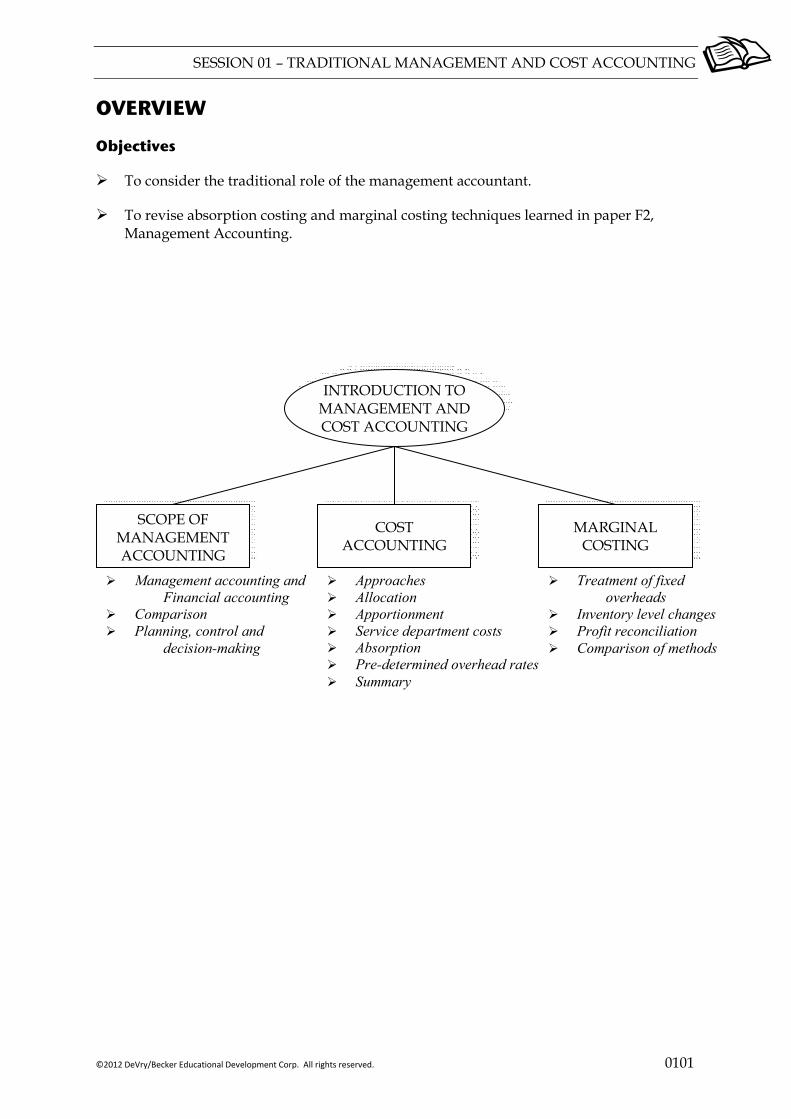
OVERVIEW
Objectives
To consider the traditional role of the management accountant.
To revise absorption costing and marginal costing techniques learned in paper F2, Management Accounting.
COST ACCOUNTING
SCOPE OF MANAGEMENT ACCOUNTING
INTRODUCTION TO MANAGEMENT AND COST ACCOUNTING
MARGINAL COSTING
Management accounting and Financial accounting
Comparison Planning, control and
decision-making
Approaches Allocation Apportionment Service department costs Absorption Pre-determined overhead rates Summary
Treatment of fixed overheads
Inventory level changes Profit reconciliation Comparison of methods
SESSION 01 – TRADITIONAL MANAGEMENT AND COST ACCOUNTING
0102 ©2012 DeVry/Becker Educational Development Corp. All rights reserved.
1 SCOPE OF TRADITIONAL MANAGEMENT ACCOUNTING
Commentary The material in this session is background information, and is not likely to feature largely in the F5 exam. However, an understanding of absorption costing is necessary to understand activity based costing which is covered in session 2. It is likely that exam questions will require candidates to compare and contrast traditional absorption costing with activity based costing.
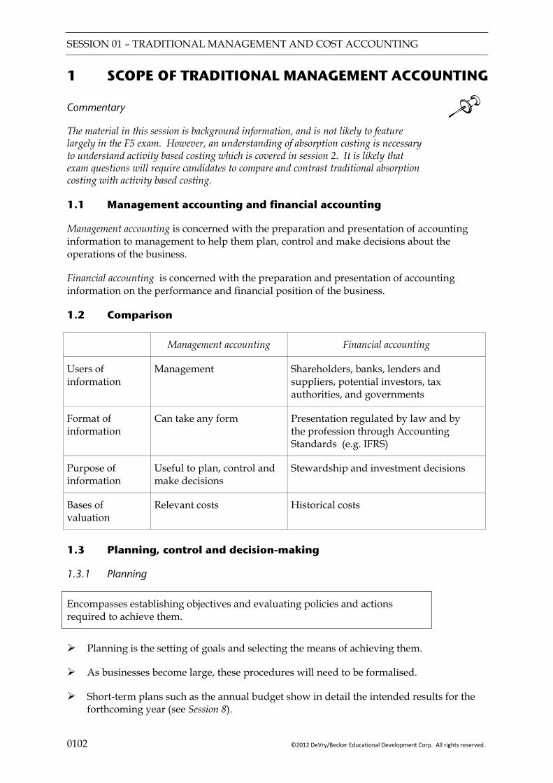
1.1 Management accounting and financial accounting
Management accounting is concerned with the preparation and presentation of accounting information to management to help them plan, control and make decisions about the operations of the business.
Financial accounting is concerned with the preparation and presentation of accounting information on the performance and financial position of the business.
1.2 Comparison
Management accounting Financial accounting
Users of information
Management Shareholders, banks, lenders and suppliers, potential investors, tax authorities, and governments
Format of information
Can take any form Presentation regulated by law and by the profession through Accounting Standards (e.g. IFRS)
Purpose of information
Useful to plan, control and make decisions
Stewardship and investment decisions
Bases of valuation
Relevant costs Historical costs
1.3 Planning, control and decision-making
1.3.1 Planning
Encompasses establishing objectives and evaluating policies and actions required to achieve them.
Planning is the setting of goals and selecting the means of achieving them.
As businesses become large, these procedures will need to be formalised.
Short-term plans such as the annual budget show in detail the intended results for the forthcoming year (see Session 8).
SESSION 01 – TRADITIONAL MANAGEMENT AND COST ACCOUNTING
©2012 DeVry/Becker Educational Development Corp. All rights reserved. 0103
Long-term plans (also called “strategic” plans) are usually documents showing the long-term objectives of the business.
1.3.2 Control
Control means checking that an organisation is on track to meet its long and short term objectives, and taking action to correct any deviations from these.
Long term control includes strategic performance evaluation, which aims to measure how the organisation is performing against its strategic objectives
Short term control focuses on comparing the budgeted results with actual results.
This usually takes the form of an operating statement which breaks down the difference into its component parts (variances). (See Sessions 10 & 11.)
1.3.3 Decision-making
Decision-making usually involves using the information provided by the costing system to make decisions (see Sessions 3 to 7).
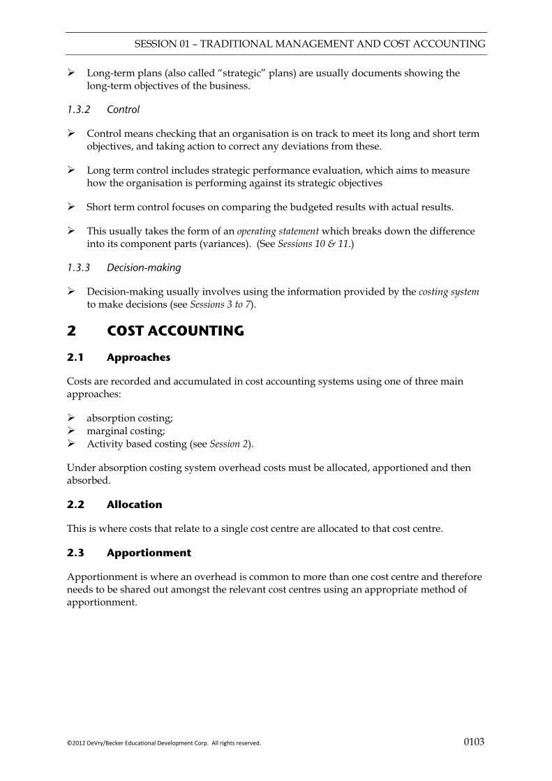
2 COST ACCOUNTING
2.1 Approaches
Costs are recorded and accumulated in cost accounting systems using one of three main approaches:
absorption costing; marginal costing; Activity based costing (see Session 2).
Under absorption costing system overhead costs must be allocated, apportioned and then absorbed.
2.2 Allocation
This is where costs that relate to a single cost centre are allocated to that cost centre.
2.3 Apportionment
Apportionment is where an overhead is common to more than one cost centre and therefore needs to be shared out amongst the relevant cost centres using an appropriate method of apportionment.
SESSION 01 – TRADITIONAL MANAGEMENT AND COST ACCOUNTING
0104 ©2012 DeVry/Becker Educational Development Corp. All rights reserved.
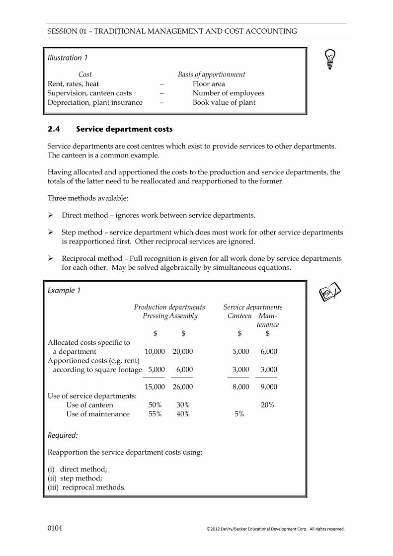
Illustration 1
Cost Basis of apportionment Rent, rates, heat − Floor area Supervision, canteen costs − Number of employees Depreciation, plant insurance − Book value of plant
2.4 Service department costs
Service departments are cost centres which exist to provide services to other departments. The canteen is a common example.
Having allocated and apportioned the costs to the production and service departments, the totals of the latter need to be reallocated and reapportioned to the former.
Three methods available:
Direct method – ignores work between service departments.
Step method – service department which does most work for other service departments is reapportioned first. Other reciprocal services are ignored.
Reciprocal method – Full recognition is given for all work done by service departments for each other. May be solved algebraically by simultaneous equations.
Example 1
Production departments Service departments Pressing Assembly Canteen Main- tenance $ $ $ $ Allocated costs specific to a department 10,000 20,000 5,000 6,000 Apportioned costs (e.g. rent) according to square footage 5,000 6,000 3,000 3,000 ______ ______ ______ ______ 15,000 26,000 8,000 9,000 Use of service departments: Use of canteen 50% 30% 20% Use of maintenance 55% 40% 5%
Required:
Reapportion the service department costs using:
(i) direct method; (ii) step method; (iii) reciprocal methods.

SESSION 01 – TRADITIONAL MANAGEMENT AND COST ACCOUNTING
©2012 DeVry/Becker Educational Development Corp. All rights reserved. 0105
Solution
(i) Direct method
Pressing Assembly Canteen Maintenance $ $ $ $ Canteen (50:30)
Maintenance (55:40)
15,000
26,000
8,000
9,000
______ ______
______ ______
______ ______
______ ______
(ii) Step (down) method
Pressing Assembly Canteen Maintenance $ $ $ $ Canteen (50:30:20)
15,000
26,000
8,000
9,000
______ ______ ______ ______
Maintenance (55:40)
______ ______
______ ______
______ ______
______ ______
(iii) Reciprocal method
Repeated distribution also Pressing Assembly Canteen Maintenance $ $ $ $ Canteen (50:30:20)
15,000
26,000
8,000
9,000
_______ _______ Maintenance (55:40:5)
_______ _______ Canteen (50:30:20)
_______ _______ Maintenance (55:40:5)
_______ _______ Canteen (50:30:20)
_______ _______
_______ _______
_______ _______
_______ _______
SESSION 01 – TRADITIONAL MANAGEMENT AND COST ACCOUNTING
0106 ©2012 DeVry/Becker Educational Development Corp. All rights reserved.
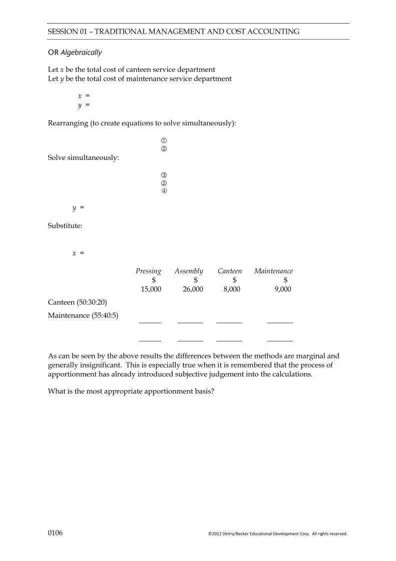
OR Algebraically
Let x be the total cost of canteen service department Let y be the total cost of maintenance service department
x = y =
Rearranging (to create equations to solve simultaneously):
Solve simultaneously:
y = Substitute:
x =
Pressing Assembly Canteen Maintenance $ $ $ $
Canteen (50:30:20)
Maintenance (55:40:5)
15,000
26,000
8,000
9,000
______ ______
_______ _______
_______ _______
_______ _______
As can be seen by the above results the differences between the methods are marginal and generally insignificant. This is especially true when it is remembered that the process of apportionment has already introduced subjective judgement into the calculations.
What is the most appropriate apportionment basis?
SESSION 01 – TRADITIONAL MANAGEMENT AND COST ACCOUNTING
©2012 DeVry/Becker Educational Development Corp. All rights reserved. 0107
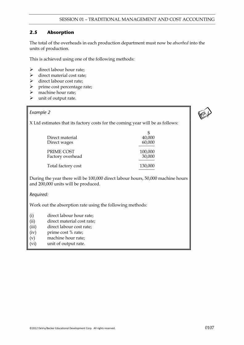
2.5 Absorption
The total of the overheads in each production department must now be absorbed into the units of production.
This is achieved using one of the following methods:
direct labour hour rate; direct material cost rate; direct labour cost rate; prime cost percentage rate; machine hour rate; unit of output rate.
Example 2
X Ltd estimates that its factory costs for the coming year will be as follows:
$ Direct material 40,000 Direct wages 60,000 _______ PRIME COST 100,000 Factory overhead 30,000 _______ Total factory cost 130,000 _______ During the year there will be 100,000 direct labour hours, 50,000 machine hours and 200,000 units will be produced.
Required:
Work out the absorption rate using the following methods:
(i) direct labour hour rate; (ii) direct material cost rate; (iii) direct labour cost rate; (iv) prime cost % rate; (v) machine hour rate; (vi) unit of output rate.

SESSION 01 – TRADITIONAL MANAGEMENT AND COST ACCOUNTING
0108 ©2012 DeVry/Becker Educational Development Corp. All rights reserved.
Solution
(i) Direct labour hour rate
(ii) Direct material cost rate
(iii) Direct labour cost rate
(iv) Prime cost % rate
(v) Machine hour rate
(vi) Unit of output rate
2.6 Pre-determined overhead rates
As the above figures have been calculated using estimates of costs for the coming year, it is known as a pre-determined overhead absorption rate (POAR). This is then used to apportion the overheads to the products. This rate is generally derived from the budgeted overhead and the normal level of production figures, in order to avoid distortion caused by seasonal fluctuations and to provide a consistent basis for measuring costs.
Finally there are three relevant figures relating to overheads:
originally budgeted overhead; actual overhead spent; overhead absorbed (POAR × Actual activity level).
The difference between (2) and (3) is the under or over absorption which will be adjusted for in the income statement for the period.
> = under-absorption – debit to income statement > = over-absorption – credit to income statement

SESSION 01 – TRADITIONAL MANAGEMENT AND COST ACCOUNTING
©2012 DeVry/Becker Educational Development Corp. All rights reserved. 0109
2.7 Summary
The diagram below shows the process described above:
PRODUCTION OVERHEADS
PRODUCTION COST
PRODUCTION DEPARTMENT B
SERVICE DEPARTMENT
DIRECT COSTS
Allocation Apportionment Reapportionment Absorption Charging of direct costs
PRODUCTION DEPARTMENT B
SESSION 01 – TRADITIONAL MANAGEMENT AND COST ACCOUNTING
0110 ©2012 DeVry/Becker Educational Development Corp. All rights reserved.
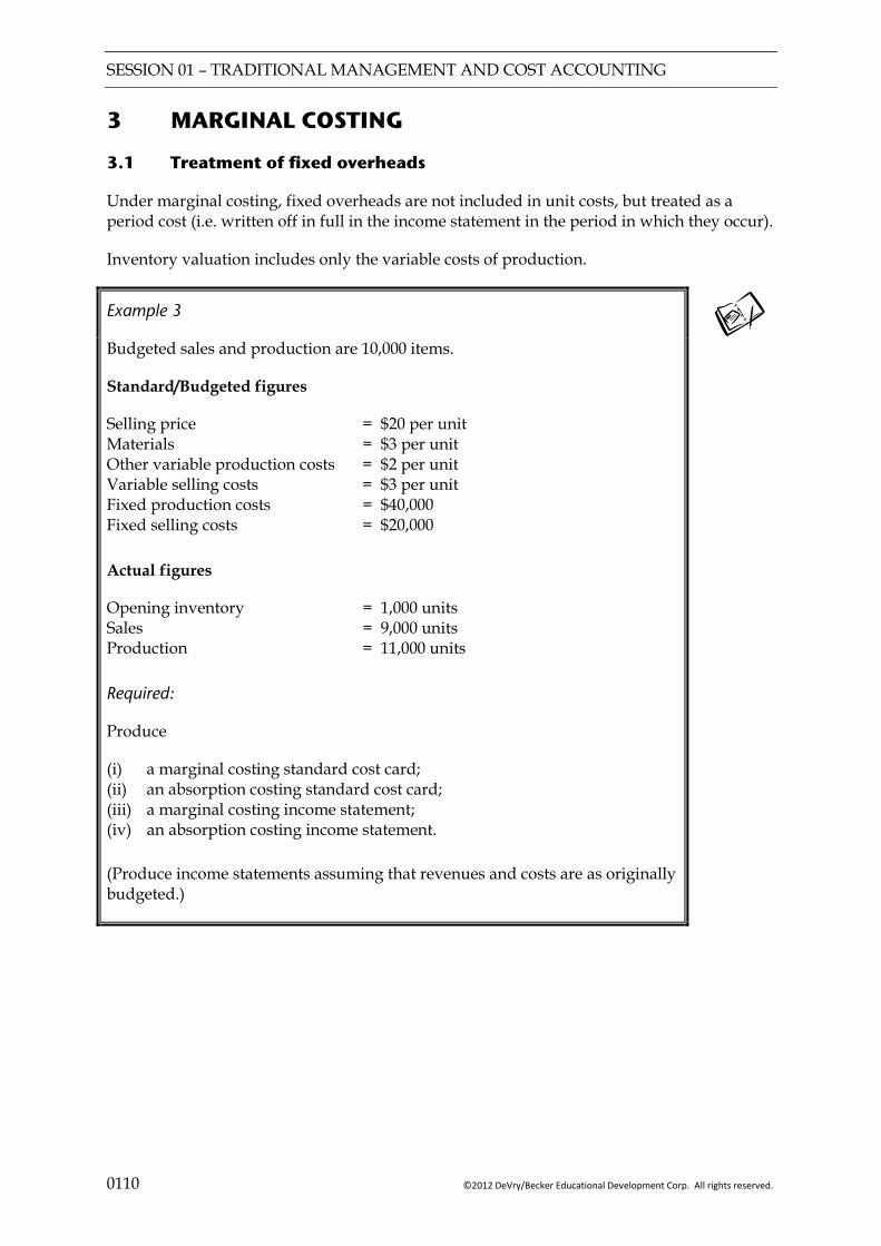
3 MARGINAL COSTING
3.1 Treatment of fixed overheads
Under marginal costing, fixed overheads are not included in unit costs, but treated as a period cost (i.e. written off in full in the income statement in the period in which they occur).
Inventory valuation includes only the variable costs of production.
Example 3
Budgeted sales and production are 10,000 items.
Standard/Budgeted figures
Selling price = $20 per unit Materials = $3 per unit Other variable production costs = $2 per unit Variable selling costs = $3 per unit Fixed production costs = $40,000 Fixed selling costs = $20,000
Actual figures
Opening inventory = 1,000 units Sales = 9,000 units Production = 11,000 units
Required:
Produce
(i) a marginal costing standard cost card; (ii) an absorption costing standard cost card; (iii) a marginal costing income statement; (iv) an absorption costing income statement.
(Produce income statements assuming that revenues and costs are as originally budgeted.)
SESSION 01 – TRADITIONAL MANAGEMENT AND COST ACCOUNTING
©2012 DeVry/Becker Educational Development Corp. All rights reserved. 0111
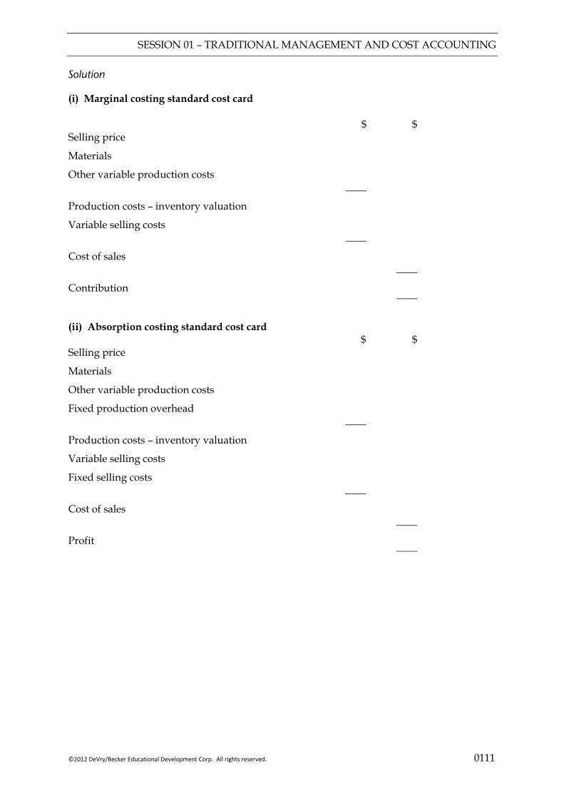
Solution
(i) Marginal costing standard cost card $ $ Selling price
Materials
Other variable production costs
____ Production costs – inventory valuation
Variable selling costs
____ Cost of sales
Contribution
____ ____
(ii) Absorption costing standard cost card $ $ Selling price
Materials
Other variable production costs
Fixed production overhead
____ Production costs – inventory valuation
Variable selling costs
Fixed selling costs
____ Cost of sales
Profit
____ ____

SESSION 01 – TRADITIONAL MANAGEMENT AND COST ACCOUNTING
0112 ©2012 DeVry/Becker Educational Development Corp. All rights reserved.
(iii) Marginal costing income statement $000 $000 Sales
Less: Cost of sales
Opening inventory †
Variable production costs
Closing inventory †
____ ____ Variable selling and administrative costs
____ Contribution
Fixed production costs
Fixed selling and administrative costs
Net profit
____ ____
† Inventory valued at variable production cost per unit only.
(iv) Absorption costing income statement $000 $000 Sales
Less: Cost of sales
Opening inventory*
Variable production costs
Fixed production costs
Closing inventory*
____ ____ Gross profit
Fixed selling and administrative costs
Variable selling and administrative costs
Net profit
____ ____
* Inventory valued at variable production cost plus fixed production cost per unit.

SESSION 01 – TRADITIONAL MANAGEMENT AND COST ACCOUNTING
©2012 DeVry/Becker Educational Development Corp. All rights reserved. 0113
An alternative layout of the absorption costing income statement, which clearly shows the over or under-absorption of overheads, would be as follows:
$000 $000
Sales
Opening inventory
Total production costs Closing inventory
____ ____
Under/over absorption
Overhead absorbed Overhead spent
____
Over absorption
____
Gross profit
Fixed selling and administrative costs
Variable selling and administrative costs
Net profit
____ ____
Example 4
$ Direct variable costs 7 Fixed production overheads 5 __ Total cost 12 __
Selling price 20
Opening inventory 1,000 units
Production 8,000 units per month
Sales Month 1 6,000 units Month 2 8,500 units Month 3 8,000 units
Required:
Produce income statements for months 1–3 using:
(a) total absorption costing; (b) marginal costing.

SESSION 01 – TRADITIONAL MANAGEMENT AND COST ACCOUNTING
0114 ©2012 DeVry/Becker Educational Development Corp. All rights reserved.
Solution
(a) Absorption costing
Month 1 Month 2 Month 3 $ $ $ $ $ $ Sales
Opening inventory
Variable production costs
Fixed production costs
Closing inventory
_______ _______ _______
Cost of goods sold
Gross profit
_______ _______
_______ _______
_______ _______
(b) Marginal costing
Month 1 Month 2 Month 3 $ $ $ $ $ $ Sales
Opening inventory
Variable production costs
Closing inventory
_______ _______ _______
Cost of goods sold
_______ _______ _______
CONTRIBUTION
Fixed production costs
Gross profit
_______ _______
_______ _______
_______ _______
3.2 Inventory level changes
Change in inventory Effect on profit
(1) (2) (3)
Closing inventory > Opening inventory Closing inventory = Opening inventory Closing inventory < Opening inventory
TAC profit > MC profit TAC profit = MC profit TAC profit < MC profit

SESSION 01 – TRADITIONAL MANAGEMENT AND COST ACCOUNTING
©2012 DeVry/Becker Educational Development Corp. All rights reserved. 0115
3.3 Profit reconciliation
Using Example 4 figures: Month 1 Month 2 Month3 $ $ $ Marginal cost profit 38,000 70,500 64,000 Difference in profit (Change in stock level × Fixed prodn o/h per unit) 2,000 × $5 500 × $5 10,000 (2,500) − ______ ______ ______ Absorption cost profit 48,000 68,000 64,000 ______ ______ ______
The above profit reconciliation assumes that the fixed overhead absorption rate per unit remains constant. If this were to change, the reconciling difference would become the difference between fixed production costs:
(i) b/f in opening inventory; and (ii) c/f in closing inventory.
3.4 Comparison of methods
Total absorption costing Marginal costing
Inventory valuation Conforms to accounting standards
Prudent valuation
Profits Depends on sales and production (manipulate it by over-inventorying)
Depends on sales
Costing procedures Avoids splitting semi-variable costs
Avoids allocation, apportionment and absorption
Decision-making Pricing More useful and relevant
Cost control Focuses on all costs Focuses on controllable costs
SESSION 01 – TRADITIONAL MANAGEMENT AND COST ACCOUNTING
0116 ©2012 DeVry/Becker Educational Development Corp. All rights reserved.
Key points
Management accounting is concerned with the preparation and presentation of accounting information to assist management to plan, control and make decisions.
Costing involves calculating the unit cost of a product or service. Traditional methods are absorption costing and marginal costing.
Under absorption costing, a share of fixed production overheads is included in the unit cost. Steps used in absorption costing are:
As fixed overheads are incurred, they are allocated to, or apportioned between the cost centres in the factory.
Overheads of the service cost centres are apportioned between the production cost centres.
Total costs in each production cost centre are absorbed into the unit cost using an appropriate basis (e.g. labour or machine hours).
Overhead absorption rates may be calculated in advance of an accounting period, based on budgeted amounts. At the end of the year, the difference between actual fixed overheads and absorbed overheads is written off to the income statement.
Marginal costing means that fixed overheads are not absorbed into unit costs. They are treated as period costs and written off to the income statement in the period in which they occur.
Profit figures based on absorption costing may differ from profits based on marginal costing. The difference is due to inventory valuation.
FOCUS
You should now be able to:
outline and distinguish between the nature and scope of management accounting and
the role of costing in meeting the needs of management;
describe the purpose of costing as an aid to planning, monitoring and controlling business activity;
explain the potential for different costing approaches to influence cost accumulation and profit reporting;
explain the requirement to allocate overheads;
describe, explain and apply absorption and marginal costing;
reconcile the resulting profits/losses from absorption and marginal costing;
SESSION 01 – TRADITIONAL MANAGEMENT AND COST ACCOUNTING
©2012 DeVry/Becker Educational Development Corp. All rights reserved. 0117
EXAMPLE SOLUTIONS
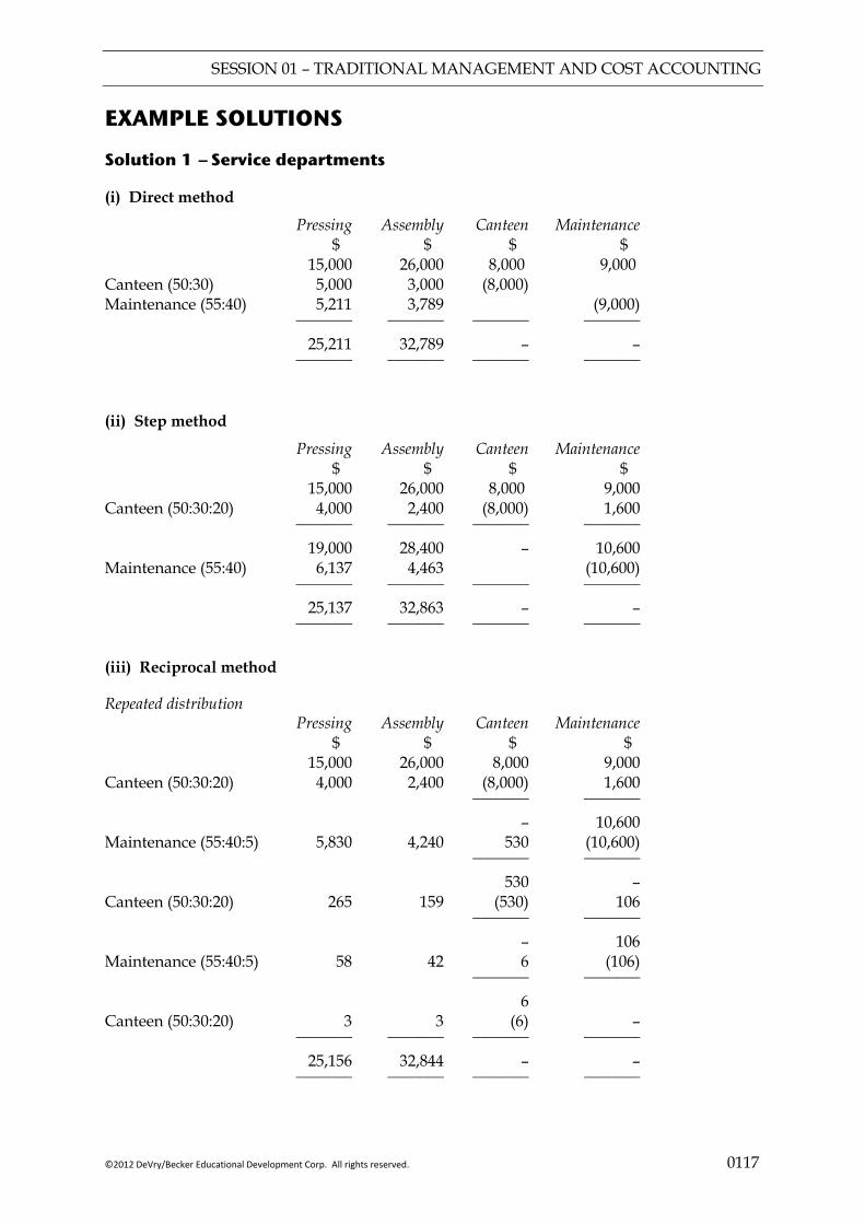
Solution 1 — Service departments
(i) Direct method
Pressing Assembly Canteen Maintenance $ $ $ $ Canteen (50:30) Maintenance (55:40)
15,000 5,000 5,211
26,000 3,000 3,789
8,000 (8,000)
9,000
(9,000) _______
25,211 _______
_______ 32,789 _______
_______ – _______
_______ – _______
(ii) Step method
Pressing Assembly Canteen Maintenance $ $ $ $ Canteen (50:30:20)
15,000 4,000
26,000 2,400
8,000 (8,000)
9,000 1,600
_______ _______ _______ _______ 19,000 28,400 – 10,600 Maintenance (55:40) 6,137 4,463 (10,600) _______
25,137 _______
_______ 32,863 _______
_______ – _______
_______ – _______
(iii) Reciprocal method
Repeated distribution Pressing Assembly Canteen Maintenance $ $ $ $ Canteen (50:30:20)
15,000 4,000
26,000 2,400
8,000 (8,000)
9,000 1,600
_______ _______ Maintenance (55:40:5)
5,830
4,240
– 530
10,600 (10,600)
_______ _______ Canteen (50:30:20)
265
159
530 (530)
– 106
_______ _______ Maintenance (55:40:5)
58
42
– 6
106 (106)
_______ _______ Canteen (50:30:20)
3
3
6 (6)
–
_______ 25,156 _______
_______ 32,844 _______
_______ – _______
_______ – _______
SESSION 01 – TRADITIONAL MANAGEMENT AND COST ACCOUNTING
0118 ©2012 DeVry/Becker Educational Development Corp. All rights reserved.
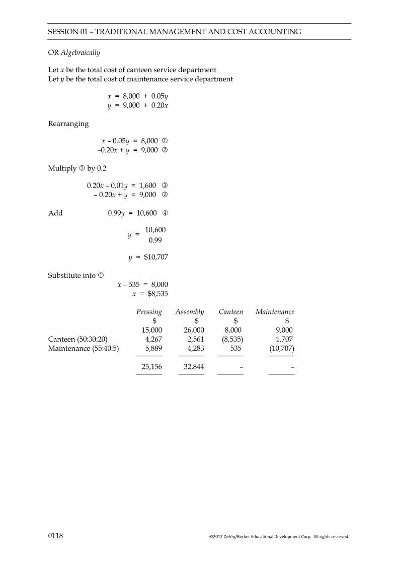
OR Algebraically
Let x be the total cost of canteen service department Let y be the total cost of maintenance service department
x = 8,000 + 0.05y y = 9,000 + 0.20x
Rearranging
x – 0.05y = 8,000 –0.20x + y = 9,000
Multiply by 0.2
0.20x – 0.01y = 1,600 – 0.20x + y = 9,000
Add 0.99y = 10,600
y = 99.0600,10
y = $10,707 Substitute into x – 535 = 8,000
x = $8,535
Pressing Assembly Canteen Maintenance $ $ $ $ Canteen (50:30:20) Maintenance (55:40:5)
15,000 4,267 5,889
26,000 2,561 4,283
8,000 (8,535)
535
9,000 1,707
(10,707) _______
25,156 _______
_______ 32,844 _______
_______ – _______
_______ – _______
SESSION 01 – TRADITIONAL MANAGEMENT AND COST ACCOUNTING
©2012 DeVry/Becker Educational Development Corp. All rights reserved. 0119
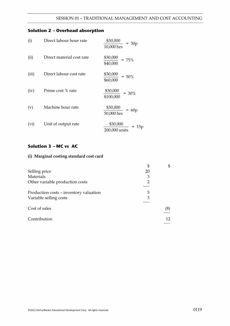
Solution 2 — Overhead absorption
(i) Direct labour hour rate hrs 10,000
$30,000 = 30p
(ii) Direct material cost rate 00040$00030$
,, = 75%
(iii) Direct labour cost rate 00060$00030$
,, = 50%
(iv) Prime cost % rate 000100$
00030$,, = 30%
(v) Machine hour rate hrs 00050
00030$,
, = 60p
(vi) Unit of output rate units 000200
000$30,
, = 15p
Solution 3 — MC vs AC
(i) Marginal costing standard cost card
$ $ Selling price 20 Materials Other variable production costs
3 2
___ Production costs – inventory valuation Variable selling costs
5 3
___ Cost of sales (8) Contribution
___ 12 ___
SESSION 01 – TRADITIONAL MANAGEMENT AND COST ACCOUNTING
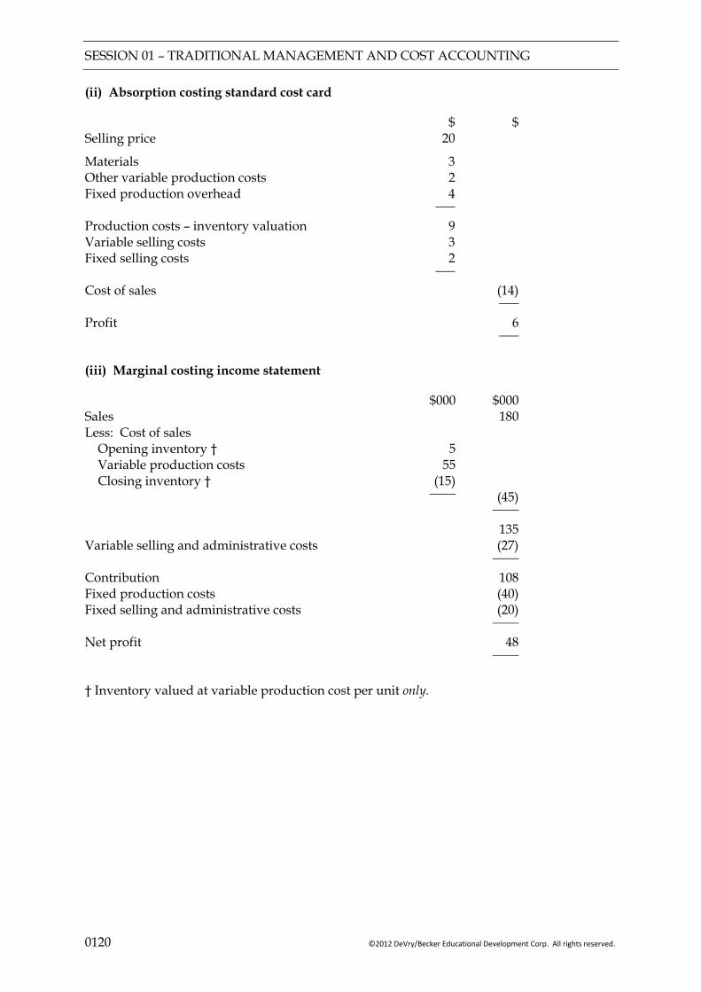
0120 ©2012 DeVry/Becker Educational Development Corp. All rights reserved.
(ii) Absorption costing standard cost card
$ $ Selling price 20
Materials Other variable production costs Fixed production overhead
3 2 4
___ Production costs – inventory valuation Variable selling costs Fixed selling costs
9 3 2
___ Cost of sales (14) Profit
___ 6 ___
(iii) Marginal costing income statement
$000 $000 Sales 180 Less: Cost of sales Opening inventory † Variable production costs Closing inventory †
5 55
(15)
____ (45) ____ 135 Variable selling and administrative costs (27) ____ Contribution Fixed production costs Fixed selling and administrative costs
108 (40) (20)
Net profit
____ 48 ____
† Inventory valued at variable production cost per unit only.
SESSION 01 – TRADITIONAL MANAGEMENT AND COST ACCOUNTING
©2012 DeVry/Becker Educational Development Corp. All rights reserved. 0121
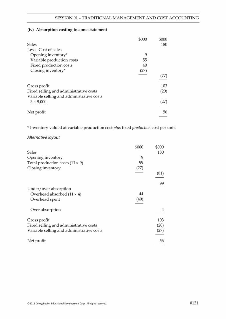
(iv) Absorption costing income statement
$000 $000 Sales 180 Less: Cost of sales Opening inventory* Variable production costs Fixed production costs Closing inventory*
9 55 40
(27)
____ (77) ____ Gross profit Fixed selling and administrative costs Variable selling and administrative costs 3 × 9,000
103 (20)
(27)
Net profit
____ 56 ____
* Inventory valued at variable production cost plus fixed production cost per unit.
Alternative layout
$000 $000 Sales Opening inventory Total production costs (11 × 9) Closing inventory
9
99 (27)
180
____ (81) ____ 99 Under/over absorption Overhead absorbed (11 × 4) Overhead spent
44 (40)
____ Over absorption 4 ____ Gross profit Fixed selling and administrative costs Variable selling and administrative costs
103 (20) (27)
Net profit
____ 56 ____
SESSION 01 – TRADITIONAL MANAGEMENT AND COST ACCOUNTING
0122 ©2012 DeVry/Becker Educational Development Corp. All rights reserved.
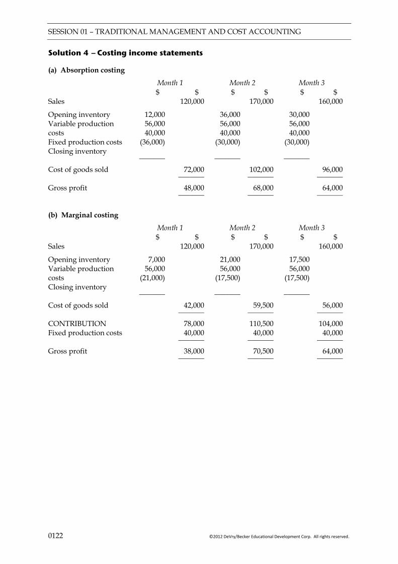
Solution 4 — Costing income statements
(a) Absorption costing
Month 1 Month 2 Month 3 $ $ $ $ $ $ Sales 120,000 170,000 160,000
Opening inventory Variable production costs Fixed production costs Closing inventory
12,000 56,000 40,000
(36,000)
36,000 56,000 40,000
(30,000)
30,000 56,000 40,000
(30,000)
_______ _______ _______ Cost of goods sold 72,000 102,000 96,000 Gross profit
_______ 48,000 _______
_______ 68,000 _______
_______ 64,000 _______
(b) Marginal costing
Month 1 Month 2 Month 3 $ $ $ $ $ $ Sales 120,000 170,000 160,000
Opening inventory Variable production costs Closing inventory
7,000 56,000
(21,000)
21,000 56,000
(17,500)
17,500 56,000
(17,500)
_______ _______ _______ Cost of goods sold 42,000 59,500 56,000 _______ _______ _______ CONTRIBUTION Fixed production costs
78,000 40,000
110,500 40,000
104,000 40,000
Gross profit
_______ 38,000 _______
_______ 70,500 _______
_______ 64,000 _______
SESSION 02 – ACTIVITY BASED COSTING
©2012 DeVry/Becker Educational Development Corp. All rights reserved. 0201
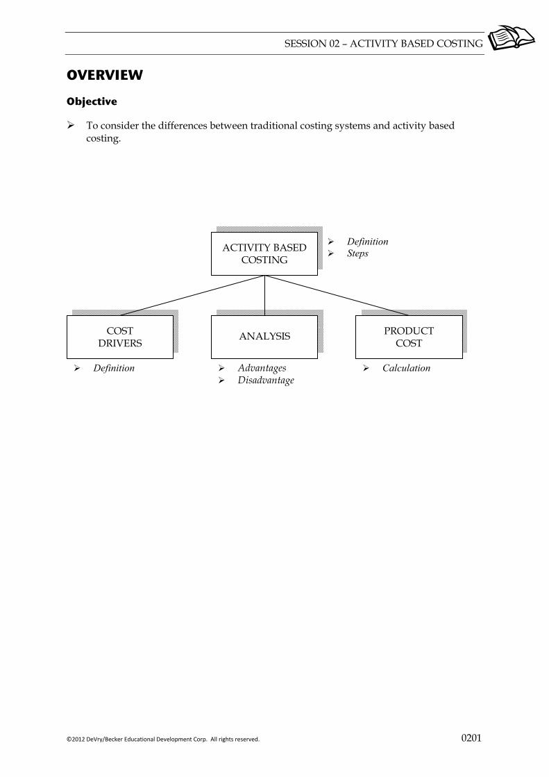
OVERVIEW
Objective
To consider the differences between traditional costing systems and activity based costing.
ACTIVITY BASED COSTING
PRODUCT COST
COST DRIVERS
ANALYSIS
Definition Steps
Definition Advantages Disadvantage
Calculation

SESSION 02 – ACTIVITY BASED COSTING
0202 ©2012 DeVry/Becker Educational Development Corp. All rights reserved.
1 ACTIVITY BASED COSTING
Definition
Activity-based costing (ABC) is an approach to costing and activity monitoring which assigns resources consumed to activities and activities to cost objects (based on estimated consumption). Cost drivers are used to apportion activity costs to output.
Commentary “ABC” as a costing method is not to be confused with ABC inventory systems.
This approach for calculating product costs was developed by Cooper and Kaplan.
It recognises that traditional ideas of fixed and variable cost categorisations are not always appropriate and that, as the proportion of overhead costs in manufacture has increased, there is a need for a more accurate method of absorbing these costs into cost units.
It looks for a clearer picture of cost behaviour and a better understanding of what determines the level of costs (i.e. “cost drivers”).
1.1 Steps
To find total product costs, overheads are traced to individual production departments, as usual, with common costs being apportioned using suitable bases.

SESSION 02 – ACTIVITY BASED COSTING
©2012 DeVry/Becker Educational Development Corp. All rights reserved. 0203
Then
Identify major activities within each
department which create cost
Determine what causes the cost of each activity – the “cost
driver”
Create a cost centre/cost pool
for each activity – the “activity cost pool”
Step 1
Step 2
Step 3
Step 4
Examples (1) Production scheduling (2) Machining (3) Despatching of orders (4) Inspections (1) Number of batch set-ups for production
scheduling (2) Machine hours for machining (3) Number of despatch orders for
despatching (4) Number of inspections Cost pool for: (1) all production scheduling costs (2) all machining costs (3) all despatching costs (4) all inspection costs Cost per (1) batch set up (2) machine hour (3) despatch order (4) inspection E.g. Product Z (1) No of batch set ups for Product Z × Cost per batch set up x (2) No of machine hours for Product Z × Cost per machine hour x (3) No of despatch orders for Product Z × Cost per despatch order x (4) No of inspections for Product Z × Cost per inspection x ___ y ___ E.g. Product Z
Overhead cost per unit = produced Zs of Noy
Calculate an absorption rate
for each “cost driver”
Calculate the total overhead cost
for manufacturing each product
Calculate overhead
cost per unit
Step 5
Step 6
Having discovered the cost drivers within the business, the original production departments may be re-organised to take advantage of potential cost savings.
SESSION 02 – ACTIVITY BASED COSTING
0204 ©2012 DeVry/Becker Educational Development Corp. All rights reserved.
2 COST DRIVERS
Definition
A factor that can causes a change in the cost of an activity.
An activity can have more than one cost driver attached to it. For example, cost drivers associated with a production activity may be:
machine operator(s); floor space occupied; power consumed; and quantity of waste and/or rejected output.
Therefore, rather than use a single absorption rate, different types of overhead cost are absorbed into units of production using more appropriate rates based on cost drivers. For example, for a particular production department the following rates may be suitable:
a warehousing cost/kg of material used; electricity cost/machine hour; production scheduling cost/production order, etc.
These can then be applied and aggregated to calculate an overhead cost per unit as set-out in Step 5 of the previous section.
3 ANALYSIS OF ABC
3.1 Advantages
Allotment of overhead is fairer and therefore product costs are more accurate.
There is a better understanding of what causes cost.
The company can concentrate on producing the most profitable items.
Control of overheads is easier, as responsibility for incoming costs must be established before ABC can be implemented.
Performance appraisal is more meaningful.
Cost driver rates can be monitored and used to identify areas of weakness or inefficiency.
Budget setting and sensitivity analysis are more accurate.
Activity based budgeting (ABB) can be used.
SESSION 02 – ACTIVITY BASED COSTING
©2012 DeVry/Becker Educational Development Corp. All rights reserved. 0205
Definition
Activity-based budgeting (ABB) is a budgeting method based on an activity framework which uses cost driver data in the processes of budget-setting and variance feedback.
New products can be designed to utilise efficient cost drivers. Cost can be designed out
of products.
When cost plus methods of pricing are used, prices based on ABC are likely to reflect more accurately the true cost of producing a product.
3.2 Disadvantages
ABC may be based on historic information but could be used for future strategic decisions.
Selection of cost drivers may not be easy.
Additional time and cost of setting up and administering the system.
Cost measurement may not be easy.
Exclusion of non-production overheads can be difficult.
Assessing the degree of completion of work in progress with respect to each cost driver is difficult.
Variance analysis is complicated.
Many judgemental decisions still required in the construction of an ABC system.

SESSION 02 – ACTIVITY BASED COSTING
0206 ©2012 DeVry/Becker Educational Development Corp. All rights reserved.
4 PRODUCT COST
4.1 Calculation
Example 1
Total budgeted fixed overheads for a firm are $712,000. These have traditionally been absorbed on a machine hour basis. The firm makes two products, A and B.
A B
Direct material cost $20 $60 Direct labour cost $50 $40 Machine time 3 hrs 4 hrs Annual output 6,000 40,000
Required:
(a) Calculate the total cost for each product on the assumption that the firm continues to absorb overheads on a machine hours’ basis.
(b) The firm is considering changing to an activity based costing system and has identified the following information:
Machine Annual Total Number of Number of hours/unit output machine hours set ups purchase orders Product A 3 6,000 18,000 16 52 Product B 4 40,000 160,000 30 100
_______ _______ _______ _______ 46,000 178,000 46 152
_______ _______ _______ _______ Cost pools: Cost driver: $ Machine related 178,000 Machine hours Set-up related 230,000 Set-ups Purchasing related 304,000 Purchase orders
_______ Total overheads 712,000
_______ Required:
Calculate the cost per unit using the ABC system.
SESSION 02 – ACTIVITY BASED COSTING
©2012 DeVry/Becker Educational Development Corp. All rights reserved. 0207
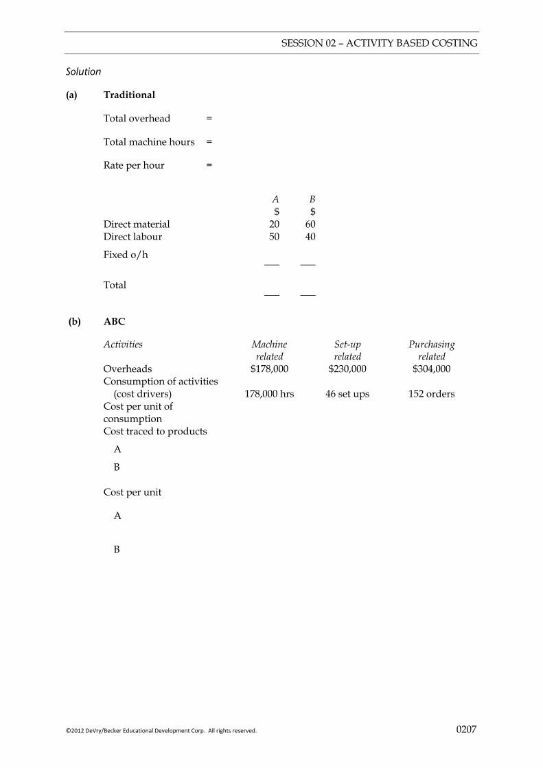
Solution
(a) Traditional
Total overhead =
Total machine hours =
Rate per hour =
A $
B $
Direct material Direct labour
20 50
60 40
Fixed o/h
___ ___ Total
___ ___ (b) ABC
Activities Machine related
Set-up related
Purchasing related
Overheads $178,000 $230,000 $304,000 Consumption of activities
(cost drivers)
178,000 hrs
46 set ups
152 orders Cost per unit of
consumption
Cost traced to products A
B
Cost per unit
A
B
SESSION 02 – ACTIVITY BASED COSTING
0208 ©2012 DeVry/Becker Educational Development Corp. All rights reserved.
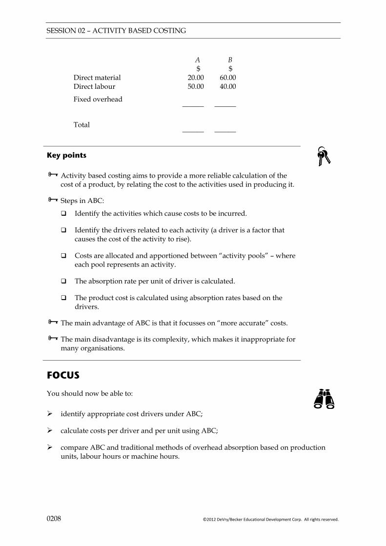
A
$ B $
Direct material Direct labour
Fixed overhead
20.00 50.00
60.00 40.00
______ ______
Total
______ ______
Key points
Activity based costing aims to provide a more reliable calculation of the cost of a product, by relating the cost to the activities used in producing it.
Steps in ABC:
Identify the activities which cause costs to be incurred.
Identify the drivers related to each activity (a driver is a factor that causes the cost of the activity to rise).
Costs are allocated and apportioned between “activity pools” – where each pool represents an activity.
The absorption rate per unit of driver is calculated.
The product cost is calculated using absorption rates based on the drivers.
The main advantage of ABC is that it focusses on “more accurate” costs.
The main disadvantage is its complexity, which makes it inappropriate for many organisations.
FOCUS
You should now be able to:
identify appropriate cost drivers under ABC;
calculate costs per driver and per unit using ABC;
compare ABC and traditional methods of overhead absorption based on production units, labour hours or machine hours.
SESSION 02 – ACTIVITY BASED COSTING
©2012 DeVry/Becker Educational Development Corp. All rights reserved. 0209
EXAMPLE SOLUTIONS
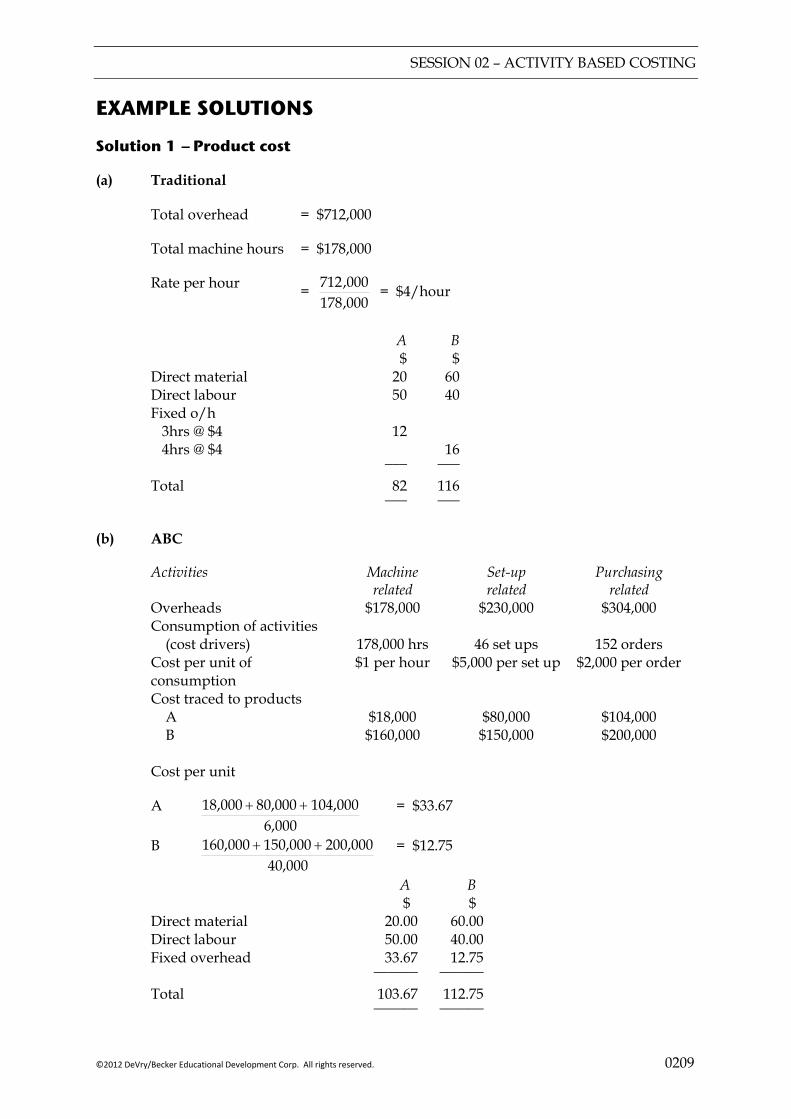
Solution 1 — Product cost
(a) Traditional
Total overhead = $712,000
Total machine hours = $178,000
Rate per hour = 000,178000,712 = $4/hour
A
$ B $
Direct material Direct labour
20 50
60 40
Fixed o/h 3hrs @ $4
4hrs @ $4 12
16 ___ ___ Total 82 116 ___ ___ (b) ABC
Activities Machine related
Set-up related
Purchasing related
Overheads $178,000 $230,000 $304,000 Consumption of activities
(cost drivers)
178,000 hrs
46 set ups
152 orders Cost per unit of
consumption $1 per hour $5,000 per set up $2,000 per order
Cost traced to products A
B $18,000 $160,000
$80,000 $150,000
$104,000 $200,000
Cost per unit
A 6,000
104,000 80,000 18,000 ++ = $33.67
B 40,000
200,000 150,000 160,000 ++ = $12.75
A $
B $
Direct material Direct labour Fixed overhead
20.00 50.00 33.67
60.00 40.00 12.75
______ ______
Total 103.67 112.75 ______ ______

SESSION 02 – ACTIVITY BASED COSTING
0210 ©2012 DeVry/Becker Educational Development Corp. All rights reserved.
SESSION 03 – DEVELOPMENTS IN MANAGEMENT ACCOUNTING
©2012 DeVry/Becker Educational Development Corp. All rights reserved. 0301
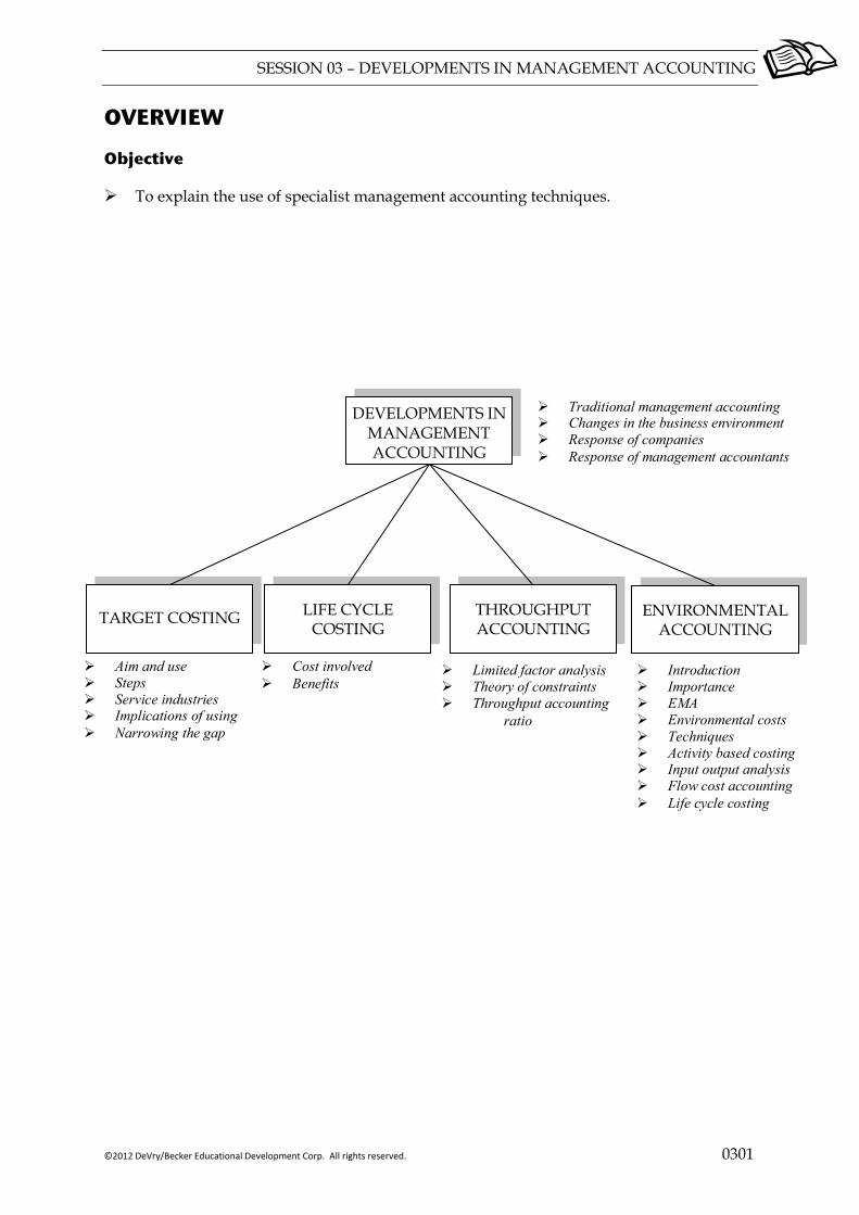
OVERVIEW
Objective
To explain the use of specialist management accounting techniques.
TARGET COSTING
Traditional management accounting Changes in the business environment Response of companies Response of management accountants
THROUGHPUT ACCOUNTING
DEVELOPMENTS IN MANAGEMENT ACCOUNTING
Aim and use Steps Service industries Implications of using Narrowing the gap
LIFE CYCLE COSTING
Limited factor analysis Theory of constraints Throughput accounting
ratio
Cost involved Benefits
ENVIRONMENTAL ACCOUNTING
Introduction Importance EMA Environmental costs Techniques Activity based costing Input output analysis Flow cost accounting Life cycle costing

SESSION 03 – DEVELOPMENTS IN MANAGEMENT ACCOUNTING
0302 ©2012 DeVry/Becker Educational Development Corp. All rights reserved.
1 DEVELOPMENTS IN MANAGEMENT ACCOUNTING
1.1 Traditional management accounting
Traditional management accounting was inward looking, focusing on controlling costs. You are already familiar with many of the techniques used in traditional management accounting from earlier papers. The most important of these are:
Costing systems (marginal and absorption costing); Budgeting systems; Standard costing and variance analysis; Working capital management
1.2 Changes in the business environment
During the 1950s and 1960s, the Western industrialised nations enjoyed strong positions in international markets. There was little competition either on price or quality. Businesses could continue to be successful by just continuing to do what they had always done. During the 1970s however, this stable business world began to disappear:
Less protection in home markets and increased globalisation led to increased competition from newly emerging industrialised nations (particularly Japan).
Introduction of computerised manufacturing systems led to the opportunity to reduce manufacturing costs while increasing quality of products.
Products’ life cycles began to fall so there was increased demand for new products from consumers.
The growth of service industries.
Business combinations resulted in larger multi-national organisations with diverse operations.
Change in the structure of business with more decentralised decision making.
1.3 Response of companies
Two developments in the commercial world are worth specific mention:
1.3.1 Total Quality Management (TQM)
Definition
Total quality management consists of continuous improvement in activities involving everyone in the organisation, managers and workers, in a totally integrated effort towards improving performance at every level.
Commentary TQM is a philosophy of getting it right first time. It is recognised that the costs of bad quality may exceed the costs of good quality. Quality is considered in more detail in a later session.
SESSION 03 – DEVELOPMENTS IN MANAGEMENT ACCOUNTING
©2012 DeVry/Becker Educational Development Corp. All rights reserved. 0303
1.3.2 Weaknesses of traditional western approach
The traditional western approach to manufacturing was to produce maximum capacity. Production was driven by internal plans rather than external demand. This led to:
Excessive holding of inventory with the associated costs of storage and obsolescence;
Delays between customer ordering products and the delivery of the products;
Bottlenecks in the production process were not highlighted;
A lack of flexibility in meeting changes in customer requirements.
1.3.3 JIT production
A just-in-time (JIT) production system is driven by the demand for finished products so each component on a production line is only produced when needed for the next stage.
A “pull through philosophy” – customer demand drives production.
Requires careful planning of demand and production requirements.
1.3.4 JIT purchasing
JIT purchasing means the receipt of materials closely with usage so that raw material stock is reduced to near zero levels.
Achieved by having a series of small production units to which stock is delivered.
A few dedicated suppliers deliver defect-free components on time two or three times per day.
1.4 Response of management accountants
In response to the changes outlined above, several new management accounting techniques have evolved. The techniques which are included in the syllabus for paper F5 are as follows:
Activity Based Costing (see previous session); Target Costing; Life Cycle Costing; Throughput Accounting.
Commentary Environmental issues are also important, so Environmental Management Accounting is covered at the end of this session.
SESSION 03 – DEVELOPMENTS IN MANAGEMENT ACCOUNTING
0304 ©2012 DeVry/Becker Educational Development Corp. All rights reserved.
2 TARGET COSTING
2.1 Aim and use
In traditional cost plus pricing models, the cost of a product is the starting point for calculating price. Having determined the unit cost of a product, a profit margin is then added to calculate the price. In a competitive world, such an approach may not be realistic. The price calculated in this way may be too high for the market to accept.
In a competitive market the price of a product may be determined by the market. Companies therefore have to accept the market price.
Target costing is an attempt to achieve an acceptable margin in a situation where the price of a product is determined externally by the market. This acceptable margin is achieved by identifying ways to reduce the costs of producing the product.
Commentary Traditionally, the cost of producing a product or service was something that companies assumed was a variable that they had little control over. More recently, Japanese companies in particular showed that no matter how efficient operations are, there are always ways to identify further cost savings. This philosophy underlies target costing.
Target costing may be used:
during the design phase of a product (where cost savings can be identified by changing the design of the product);
for existing products (where cost savings can be achieved without changing the design of the product).
2.2 Steps in target costing
(1) Determine the price which the market will accept for the product, based on market research. This may take into account the market share required.
(2) Deduct a required profit margin from this price-this gives the target cost.
(3) Estimate the actual cost of the product. If it is a new product, this will be an estimate.
(4) Identify ways to narrow the gap between the actual cost of the product and the target cost.
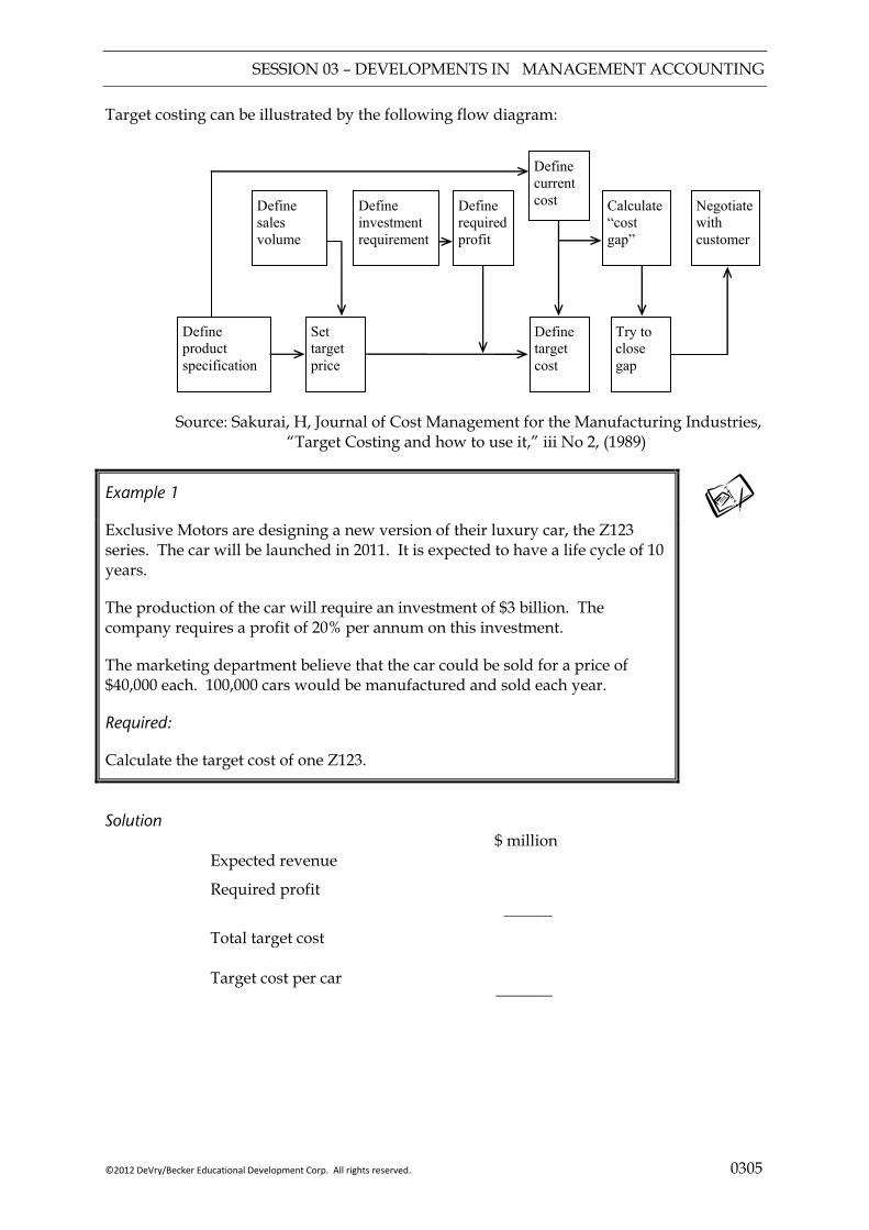
SESSION 03 – DEVELOPMENTS IN MANAGEMENT ACCOUNTING
©2012 DeVry/Becker Educational Development Corp. All rights reserved. 0305
Target costing can be illustrated by the following flow diagram:
Define sales volume
Define investment requirement
Define requiredprofit
Define current cost Calculate
“cost gap”
Negotiate with customer
Define product specification
Set target price
Define target cost
Try to close gap
Source: Sakurai, H, Journal of Cost Management for the Manufacturing Industries, “Target Costing and how to use it,” iii No 2, (1989)
Example 1
Exclusive Motors are designing a new version of their luxury car, the Z123 series. The car will be launched in 2011. It is expected to have a life cycle of 10 years.
The production of the car will require an investment of $3 billion. The company requires a profit of 20% per annum on this investment.
The marketing department believe that the car could be sold for a price of $40,000 each. 100,000 cars would be manufactured and sold each year.
Required:
Calculate the target cost of one Z123.
Solution $ million Expected revenue
Required profit
______
Total target cost Target cost per car _______
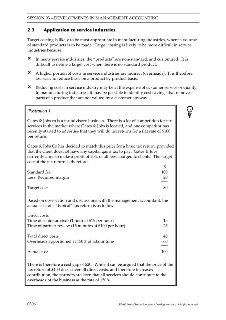
SESSION 03 – DEVELOPMENTS IN MANAGEMENT ACCOUNTING
0306 ©2012 DeVry/Becker Educational Development Corp. All rights reserved.
2.3 Application to service industries
Target costing is likely to be most appropriate in manufacturing industries, where a volume of standard products is to be made. Target costing is likely to be more difficult in service industries because:
In many service industries, the “products” are non-standard, and customised. It is difficult to define a target cost when there is no standard product.
A higher portion of costs in service industries are indirect (overheads). It is therefore less easy to reduce these on a product by product basis.
Reducing costs in service industry may be at the expense of customer service or quality. In manufacturing industries, it may be possible to identify cost savings that remove parts of a product that are not valued by a customer anyway.
Illustration 1
Gates & Jobs co is a tax advisory business. There is a lot of competition for tax services in the market where Gates & Jobs is located, and one competitor has recently started to advertise that they will do tax returns for a flat rate of $100 per return.
Gates & Jobs Co has decided to match this price for a basic tax return, provided that the client does not have any capital gains tax to pay. Gates & Jobs currently aims to make a profit of 20% of all fees charged to clients. The target cost of the tax return is therefore: $ Standard fee 100 Less: Required margin 20 ___
Target cost 80 ___
Based on observation and discussions with the management accountant, the actual cost of a “typical” tax return is as follows:
Direct costs Time of senior advisor (1 hour at $15 per hour) 15 Time of partner review (15 minutes at $100 per hour) 25 ___
Total direct costs 40 Overheads apportioned at 150% of labour time 60 ___
Actual cost 100 ___
There is therefore a cost gap of $20. While it can be argued that the price of the tax return of $100 does cover all direct costs, and therefore increases contribution, the partners are keen that all services should contribute to the overheads of the business at the rate of 150%.
SESSION 03 – DEVELOPMENTS IN MANAGEMENT ACCOUNTING
©2012 DeVry/Becker Educational Development Corp. All rights reserved. 0307
Illustration 2
Following on from Illustration 1 methods that might be used to reduce the cost gap include:
Reduce the time taken by the senior (e.g. using a software package).
Reduce partner time (e.g. the partner might not review really basic returns at all).
Reduce the overheads of the business (e.g. by using activity based costing methods to identify more accurately the drivers of overheads) and finding ways to economise.
2.4 Narrowing the target cost gap
Target costing relies on multi-disciplinary teams, which discuss ways to reduce the gap between the actual (expected) cost and the target cost.
Some methods which have been used successfully in practice are as follows:
Reconsider the design to eliminate non value added elements; Reduce the number of components or standardise components; Use less expensive materials; Employ a lower grade of staff on production; Invest in new technology; Outsource elements of the production or support activities; Reduce manning levels or redesigning the work flow.
Such methods may be assisted by the following techniques:
“Tear down analysis” (also called “reverse engineering”) – this involves examining a competitor’s product to identify possible improvements or cost reductions.
Value engineering – involves investigating the factors that affect the cost of a product or service. The aim is to improve the design of a product so that the same functions can be provided for a lower cost, or eliminating functions which the customer does not value, but which increase costs.
Functional analysis – involves identifying the attributes/functions of a product that customers value. The determination of a price that the customer is prepared to pay for each of these functions is then performed. If the cost of providing the function exceeds the value, then the function is dropped.
SESSION 03 – DEVELOPMENTS IN MANAGEMENT ACCOUNTING
0308 ©2012 DeVry/Becker Educational Development Corp. All rights reserved.
3 LIFE CYCLE COSTING
Definition
A system which tracks and accumulates the actual costs and revenues attributable to each product from development through to abandonment.
In the modern manufacturing environment a high proportion of a product’s costs will
be incurred at the early stages in its life cycle (e.g. development, design and set-up costs). However, revenues only arise when the product is actually being manufactured and sold.
Traditional financial and management accounting systems focus only on costs and revenues incurred during the manufacturing stage of the products life. They therefore ignore:
costs incurred in developing and designing the product; and any abandonment and disposal costs at the end of the product’s life.
Life cycle costing estimates and accumulates costs over the a products entire life cycle to determine whether the profits earned during the manufacturing stage will cover the costs incurred pre and post manufacturing.
It traces development, design and set-up costs to individual products over their entire life cycles.
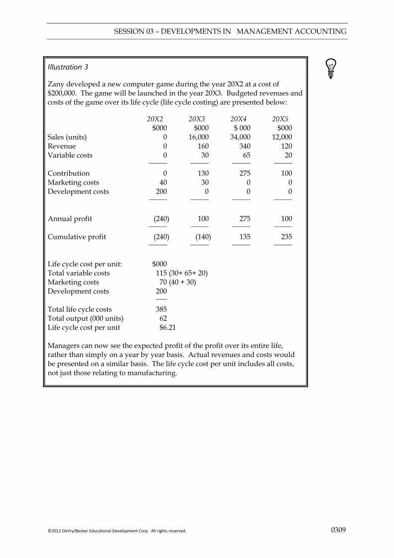
SESSION 03 – DEVELOPMENTS IN MANAGEMENT ACCOUNTING
©2012 DeVry/Becker Educational Development Corp. All rights reserved. 0309
Illustration 3
Zany developed a new computer game during the year 20X2 at a cost of $200,000. The game will be launched in the year 20X3. Budgeted revenues and costs of the game over its life cycle (life cycle costing) are presented below:
20X2 20X3 20X4 20X5 $000 $000 $ 000 $000 Sales (units) 0 16,000 34,000 12,000 Revenue 0 160 340 120 Variable costs 0 30 65 20 _____ _____ _____ _____
Contribution 0 130 275 100 Marketing costs 40 30 0 0 Development costs 200 0 0 0 _____ _____ _____ _____
Annual profit (240) 100 275 100 _____ _____ _____ _____
Cumulative profit (240) (140) 135 235 _____ _____ _____ _____
Life cycle cost per unit: $000 Total variable costs 115 (30+ 65+ 20) Marketing costs 70 (40 + 30) Development costs 200 ___ Total life cycle costs 385 Total output (000 units) 62 Life cycle cost per unit $6.21 Managers can now see the expected profit of the profit over its entire life, rather than simply on a year by year basis. Actual revenues and costs would be presented on a similar basis. The life cycle cost per unit includes all costs, not just those relating to manufacturing.

SESSION 03 – DEVELOPMENTS IN MANAGEMENT ACCOUNTING
0310 ©2012 DeVry/Becker Educational Development Corp. All rights reserved.
3.1 Cost involved at different stages of the life cycle
For the purposes of life cycle costing, three stages can be identified in the product’s life cycle:
Planning and design stage; Manufacturing stage; Service and abandonment stage.
During the planning and design phase, many of the decisions made about the products design will determine the costs that will be incurred during the future. These are committed costs. Although they are not actually incurred during the design phase the company is committed to incurring the expenditure in the future (mainly during the manufacturing stage).
Tools such as target costing (see above) may be used to reduce such committed costs, if they exceed what is acceptable.
Actual costs incurred during the planning and design phase include the costs of design, including the development of prototypes, and the cost of market research.
Marketing and advertising costs will be incurred during the manufacturing stage. These are likely to be higher at the start of the manufacturing phase as the product is new, and needs to be introduced to the market.
In some industries there may be abandonment costs as the end of the products life. In the nuclear power industry, for example, costs of decontaminating the land on which the plant is built may be high.
Clearly the pattern of expenditure will vary from industry to industry. However it is not uncommon for committed costs during the planning and design phase to reach 80% of the total costs over the product’s life.
Costs committed
Costs incurred
Planning and design stage
Manufacturing and sales stage
Service and abandonment stage
Product life cycle phase
Perc
enta
ge o
f cos
ts
100 -
70
SESSION 03 – DEVELOPMENTS IN MANAGEMENT ACCOUNTING
©2012 DeVry/Becker Educational Development Corp. All rights reserved. 0311
3.2 Benefits of life cycle costing
It encourages management to plan the pricing strategy for the whole product life, rather than on a short term basis. Pricing, and in particular, the impact of the product life cycle on pricing decisions is discussed in session 6 of this study system.
Identifying the costs that will be incurred throughout the product’s life means that management understands the costs better and therefore enables management to control them better.
By monitoring a product’s revenues and costs on a cumulative basis over the life of the product, management is provided with more meaningful information for control, than by monitoring costs and revenues on a period by period basis.
It is much easier to “design out costs” during the design phase of a product than to “control out costs” later in the product’s life cycle. By considering the whole life cycle of the product at the design phase, management is more likely to achieve reasonable cost base and therefore reasonable profits.
Decisions about whether to continue to develop and manufacture products will be based on more complete information when the product life cycle is considered. Where costs and revenues are monitored on a period by period basis, there is the risk that products in the development phase will be scrapped because they do not bring in revenues.
4 THROUGHPUT ACCOUNTING
4.1 Limited factor analysis (Key Factor Analysis)
Before covering throughput accounting ratio, it is useful to consider the basics of limited factor analysis. (This is developed further in a later session.)
In the short term, sales demand may be greater than productive capacity. For example, output may be restricted by a shortage of:
labour; materials; machinery; factory space.
Where such limiting factors apply, contribution (and therefore profit) is maximised by
using scarce resources on the product(s) which make the “best use” of them.

SESSION 03 – DEVELOPMENTS IN MANAGEMENT ACCOUNTING
0312 ©2012 DeVry/Becker Educational Development Corp. All rights reserved.
4.1.1 Method
Rule: Where resources are unlimited – make all those products which give “positive contribution”.
Rule: Where a factor of production is limited – contribution and profit because the difference is fixed costs) will be maximised by concentrating production on that product(s) which make(s) “best use” of the scarce resource.
This is the product which gives the highest contribution per unit of key (limiting) factor or resource, calculated as:
used resource scarce of Unitsunit peron Contributi
The following approach is used to decide which product(s) to make to maximise profit which means maximising contribution), where one of the factors of production is limited:
(1) Calculate contribution per key factor for each product;
(2) Rank the products according to the contribution per unit (CPU) of scarce resource calculated;
(3) Concentrate production on those products with the highest CPU of scarce resource – until all of the scarce resource is used up.
Example 2
Material I is restricted to 12,000 kilos.
Product A B C
Contribution per unit ($) 16 10 24 Kilos of I per unit 4 2 8
Required:
Calculate the maximum contribution which can be achieved.
Solution
Product A B C Contribution per unit No of kilos per unit Contribution per kilo Rank
Therefore produce
Maximum contribution =
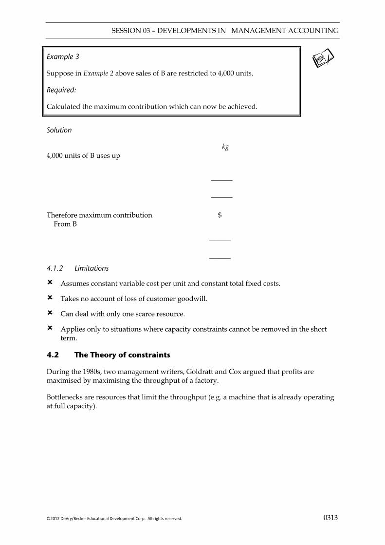
SESSION 03 – DEVELOPMENTS IN MANAGEMENT ACCOUNTING
©2012 DeVry/Becker Educational Development Corp. All rights reserved. 0313
Example 3
Suppose in Example 2 above sales of B are restricted to 4,000 units.
Required:
Calculated the maximum contribution which can now be achieved.
Solution
kg 4,000 units of B uses up
______
______ Therefore maximum contribution $ From B
______
______ 4.1.2 Limitations
Assumes constant variable cost per unit and constant total fixed costs.
Takes no account of loss of customer goodwill.
Can deal with only one scarce resource.
Applies only to situations where capacity constraints cannot be removed in the short term.
4.2 The Theory of constraints
During the 1980s, two management writers, Goldratt and Cox argued that profits are maximised by maximising the throughput of a factory.
Bottlenecks are resources that limit the throughput (e.g. a machine that is already operating at full capacity).

SESSION 03 – DEVELOPMENTS IN MANAGEMENT ACCOUNTING
0314 ©2012 DeVry/Becker Educational Development Corp. All rights reserved.
Illustration 4
A factory makes 3 products, all of which pass through 3 machines. The time spent on each machine is the same for all three products. Demand for the company’s products exceeds the amount that the company can produce. The maximum daily output of the three machines is as follows:
Machine 2 is the bottleneck, as this produces the lowest volume of output.
Goldratt and Cox proposed the following process to maximise profit when faced with bottlenecks:
(1) Identify the systems bottlenecks. In the real world this will be more complex than the simplified Illustration 4 above.
(2) Decide which products to make, given the bottlenecks. This requires limiting factor analysis using the time spent on the bottleneck as the limited factor (see Example 5 below).
(3) Ensure that other resources do not produce at a higher rate than the bottleneck. In Illustration 4, if machine 1 were to operate at its maximum capacity of 200 units per day, machine 2 would only be able to take 180 units, so 20 units of work in progress would build up.
(4) Eliminate the systems bottlenecks. This can be done for example by buying additional machines, training the machine operators, or reducing the time spent on the bottleneck resource.
(5) Once the bottleneck has been broken, another resource becomes the bottleneck. For example, if the capacity of machine 2 were increased to 240 units per day, Machine 1 would become the bottleneck. Steps 1 – 4 are repeated. The theory of constraints is therefore a process of continuous improvement.
Commentary This process they called “the theory of constraints”. The ideas above conflict with traditional management accounting:
The idea that Machine A should not operate at full capacity would lead to idle time of the operators of Machine A. Goldratt and Cox argue that this is fine as the cost of idle time is less than the cost of the work in progress that would build up if machine A were to operate at full capacity.
Machine 1 200 units
Machine 2 180 units
Machine 3 210 units

SESSION 03 – DEVELOPMENTS IN MANAGEMENT ACCOUNTING
©2012 DeVry/Becker Educational Development Corp. All rights reserved. 0315
Under traditional management accounting, the build-up of work in progress would not affect the profits of the business (since closing work in progress is part of closing inventory and deducted in determining cost of sales). Goldratt and Cox argue that this is wrong because the build-up of work in progress in front of a bottleneck is a cost to the company if the volume of work in progress is continually increasing.
Goldratt and Cox introduced the idea of “throughput contribution” as the measure of performance.
Definition
Throughput contribution is sales revenue less direct material costs.
They argue that all other costs which are traditionally treated as variable are fixed in the short run (e.g. labour). When performing limited factor analysis to determine which products to produce, given a bottleneck, they would advocate producing those products that produce maximum throughput contribution per hour of bottleneck.
Example 4a
Two products, the Ding and the Dong, are manufactured in a factory. They pass through 3 processes; process 1, process 2 and process 3. Process 2 has been identified as the bottleneck. There are 10 hours of process 2 time available per day. Information relating to the two products is as follows:
Ding Dong $ $ Selling price per unit 100 80 Direct materials per unit 70 60 Direct labour per unit 5 10 _____ _____
Traditional contribution per unit 25 10 _____ _____
Maximum demand per day 8 14 Time on process 2 per unit (hours) 1 0.5 Required:
Determine the daily production plan that would maximise:
(a) traditional contribution; and (b) throughput contribution.
State the value of each of these contributions.
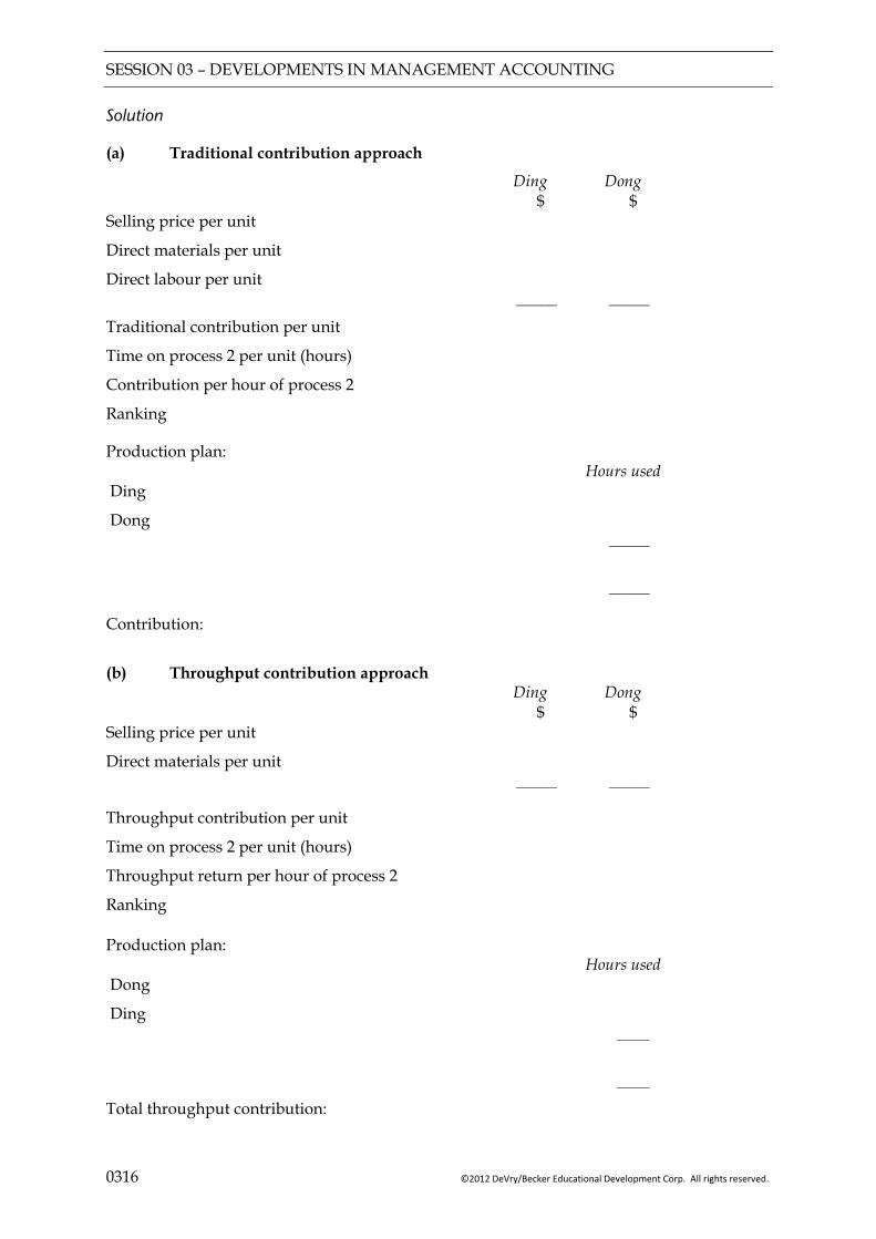
SESSION 03 – DEVELOPMENTS IN MANAGEMENT ACCOUNTING
0316 ©2012 DeVry/Becker Educational Development Corp. All rights reserved.
Solution
(a) Traditional contribution approach
Ding Dong $ $ Selling price per unit
Direct materials per unit
Direct labour per unit _____ _____
Traditional contribution per unit
Time on process 2 per unit (hours)
Contribution per hour of process 2
Ranking
Production plan: Hours used Ding
Dong
_____
_____
Contribution:
(b) Throughput contribution approach Ding Dong $ $ Selling price per unit
Direct materials per unit _____ _____
Throughput contribution per unit
Time on process 2 per unit (hours)
Throughput return per hour of process 2
Ranking Production plan: Hours used Dong
Ding
____
____ Total throughput contribution:
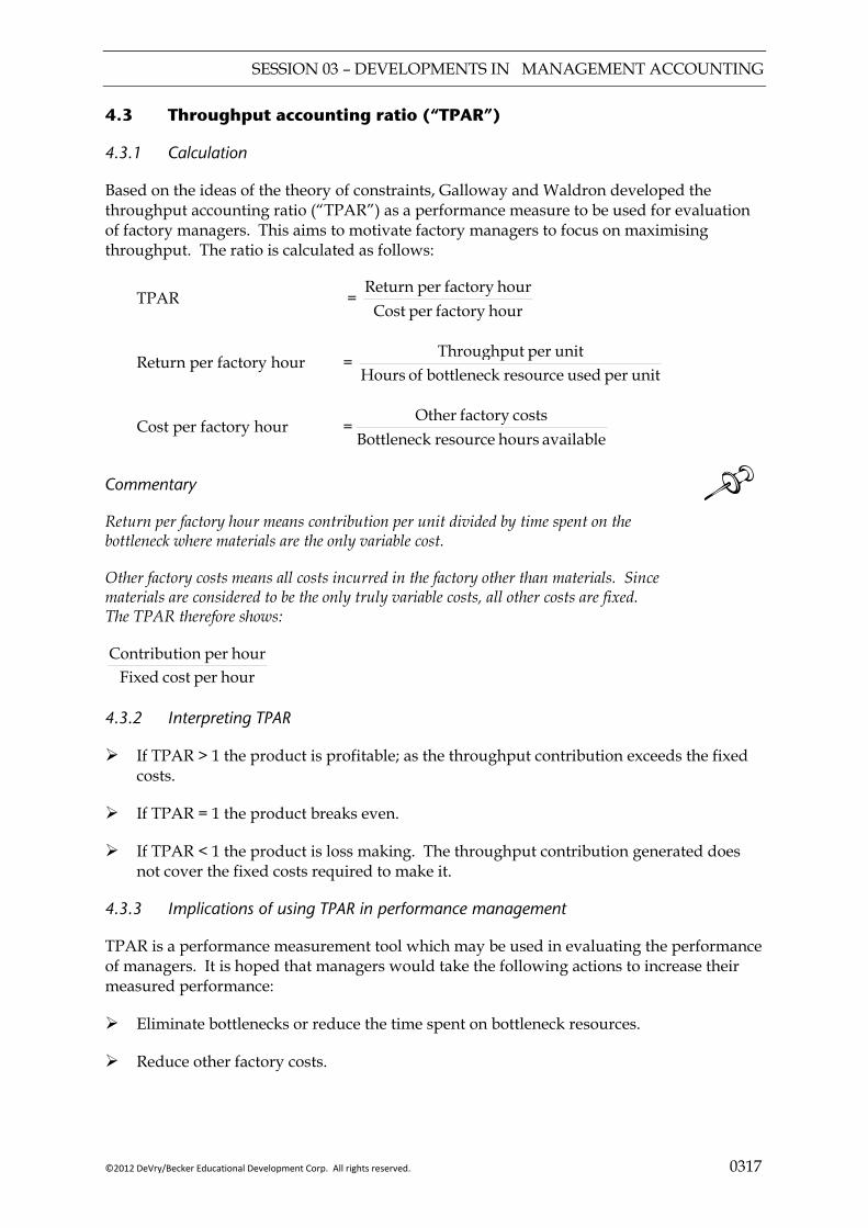
SESSION 03 – DEVELOPMENTS IN MANAGEMENT ACCOUNTING
©2012 DeVry/Becker Educational Development Corp. All rights reserved. 0317
4.3 Throughput accounting ratio (“TPAR”)
4.3.1 Calculation
Based on the ideas of the theory of constraints, Galloway and Waldron developed the throughput accounting ratio (“TPAR”) as a performance measure to be used for evaluation of factory managers. This aims to motivate factory managers to focus on maximising throughput. The ratio is calculated as follows:
TPAR = hour factory per Cost
hour factory perReturn
Return per factory hour = unit per used resource bottleneck of Hours
unit per Throughput
Cost per factory hour =available hours resource Bottleneck
costs factory Other
Commentary Return per factory hour means contribution per unit divided by time spent on the bottleneck where materials are the only variable cost.
Other factory costs means all costs incurred in the factory other than materials. Since materials are considered to be the only truly variable costs, all other costs are fixed. The TPAR therefore shows:
hour per cost Fixedhour peron Contributi
4.3.2 Interpreting TPAR
If TPAR > 1 the product is profitable; as the throughput contribution exceeds the fixed costs.
If TPAR = 1 the product breaks even.
If TPAR < 1 the product is loss making. The throughput contribution generated does not cover the fixed costs required to make it.
4.3.3 Implications of using TPAR in performance management
TPAR is a performance measurement tool which may be used in evaluating the performance of managers. It is hoped that managers would take the following actions to increase their measured performance:
Eliminate bottlenecks or reduce the time spent on bottleneck resources.
Reduce other factory costs.

SESSION 03 – DEVELOPMENTS IN MANAGEMENT ACCOUNTING
0318 ©2012 DeVry/Becker Educational Development Corp. All rights reserved.
Mathematically the ratio could also be improved by increasing selling prices or reducing material costs. In a competitive environment however, increasing selling prices may not be feasible. Reducing material costs may have implications on quality, so this may also not be desirable.
Example 5
Continuing on from Example 4. The fixed costs per day of the factory are as follows:
$ Labour costs 120 Variable overheads 180 Fixed 50 ____
Total fixed costs per day 350 ____ Required:
Calculate the TPAR for the Ding and the Dong.
5 ENVIRONMENTAL MANAGEMENT ACCOUNTING
5.1 Introduction
Over the past thirty years, environmental issues have become an area of increasing interest. Environmental activists are claiming that current human activity is causing global warming and warning of dire consequences for the planet unless we reduce our poor environmental behaviour. The most pressing issues are:
Global warming, caused by the emission of greenhouse gasses.
Many natural resources are scarce, and global reserves of these resources are being depleted. In particular, energy and water are resources that are forecast to become very scarce over the next 50 years.
Pollution is causing the loss of habitats for nature and for humans.
5.2 Importance of the environment for business
As far as business is concerned, environmental behaviour is important for the following reasons:
Poor environmental behaviour can have an adverse impact on an organisation’s image, which may lead to a loss of sales as customers boycott the organisations products.
Many governments may impose heavy fines on companies that harm the environment. Companies may also have to pay large amounts to clean up any pollution that they are responsible for.
SESSION 03 – DEVELOPMENTS IN MANAGEMENT ACCOUNTING
©2012 DeVry/Becker Educational Development Corp. All rights reserved. 0319
Increasing government regulations on environmental issues such as pollution has increased the costs of compliance for businesses.
Improving environmental behaviour can reduce costs. For example, a programme of increasing energy efficiency will lead to a reduction on depletion of natural resources, while at the same time reducing energy costs for the companies concerned.
Businesses as corporate citizens have a moral duty to play their part in helping to reduce the harm they do to the environment.
Illustration 5
The deep water horizon oil spill in April 2010 was one of the worst environmental disasters on record. An exploratory oil rig in the Gulf of Mexico exploded, leading to a partially capped oil well one mile below the surface of the water. Experts estimate that between 35,000 to 60,000 barrels of oil per day leaked from this well, depending on weather conditions. It took approximately three months to re seal the oil well and stop the leek.
BP was the majority owner of the oil field. Although the rig was operated by a sub-contractor on behalf of BP, the US Government stated that it held BP primarily responsible for the leak.
BP recognised a pre-tax cost of $40.9 billion in its 2010 financial statements relating to the oil spill (Compared to a profit for the year 2009 of $16.6. billion.) This includes a fund of $20 billion that has been set up to compensate the local community for damages caused as well as costs incurred on cleaning up the spill.
5.3 Environmental Management Accounting (EMA)
Traditional management accounting systems do not provide any analysis of environmental costs. Management are often unaware of them. The implication of this is that:
Management cannot do enough to manage their environmental activities.
Management accounts underestimate the costs of poor environmental behaviour and underestimate the benefits of good environmental behaviour.
Environmental Management Accounting aims to overcome this.
Definition
EMA is the identification, collection, analysis and use of two types of information for internal decision making; physical information on the use, flows and rates of energy, water and materials (including wastes); and monetary information on environment related costs, earnings and savings. Environmental Management Accounting Research and Information Centre EMARIC

SESSION 03 – DEVELOPMENTS IN MANAGEMENT ACCOUNTING
0320 ©2012 DeVry/Becker Educational Development Corp. All rights reserved.
It is important to remember that there are two aspects to environmental management accounting:
Physical information, which focuses on the physical use of scarce resources and how much waste occurs.
Monetary information on environment related costs, earnings and savings.
5.4 Defining environmental costs
The first step in dealing with environmental costs is to define what is meant by environmental costs. Various different definitions or categories of environmental costs have been suggested. One of these is the definitions provided by the US environmental protection agency, which identified the following categories of environmental costs:
Conventional costs: costs having environmental relevance (e.g. costs of buying energy and other scarce resources).
Potentially hidden costs are those environmental costs that are recorded, but simply included within general overheads, so management is not aware of them.
Contingent costs are potential future costs (e.g. costs of cleaning up damage caused by pollution).
Commentary In financial statements these might be disclosed as contingent liabilities or provided for if they meet the definition and recognition criteria of IAS 37 “Provisions, Contingent Liabilities and Contingent Assets”.
Image and relationship costs are the costs of producing environmental reports and
promoting the company’s environmental activities.
An alternative categorisation of environmental costs was proposed by Hansen and Mendova, who came up with a definition based on total quality management:
Environmental prevention costs are the costs of activities undertaken to prevent the production of waste (e.g. spending on redesigning processes to reduce the amount of pollution released into the atmosphere).
Environmental detection costs are those incurred to ensure that the organisation complies with regulations and voluntary standards (e.g. costs of auditing the organisation’s environmental activities).
Environmental internal failure costs are costs incurred to clean up environmental waste and pollution before it has been released into the environment (e.g. costs of disposing of toxic waste).
Environmental external failure costs are costs incurred on activities performed after discharging waste into the environment (e.g. costs of cleaning up an ocean after spilling oil).
SESSION 03 – DEVELOPMENTS IN MANAGEMENT ACCOUNTING
©2012 DeVry/Becker Educational Development Corp. All rights reserved. 0321
5.5 EMA techniques
Having identified the various types of environmental costs, it is necessary to provide useful information to management to help them to manage and control their environmental activities – with the purpose of saving money and reducing the harm caused by operation s to the environment. Various tools have been proposed for this:
An environmental cost report, based on the costs defined by Hansen and Mendova, with each category of costs shown as a percentage of revenues;
Environmental activity based costing;
Input output analysis;
Flow cost accounting;
Life cycle costing.
5.6 Environmental activity based costing
Environmental activity based costing applies activity based costing principles to environmental costs, so that the environmental costs are apportioned “correctly” to the products that use the drivers that cause the costs to be incurred.
Normally many environmental costs are hidden within general overheads and therefore apportioned to products using inappropriate drivers. This can mean that product costs do not truly reflect the environmental costs associated with making them.
Under environmental activity based costing, environmental-related costs are removed from general overheads and allocated to environmental activities. Investigation of these activities occurs to identify the key drivers of the cost. For example, one activity may be monitoring emissions. The driver of this may be production time of products using a particular process that produces emissions. The costs of monitoring emissions can then be apportioned to the products based on the amount of production time used by each product.
The main methods of allocating the environmental cost (the allocation keys) to the various activities might be the following:
Volume of emissions or waste;
Toxicity of emission and waste treated;
Volume of emission treated;
The relative costs of treating different types of emissions.
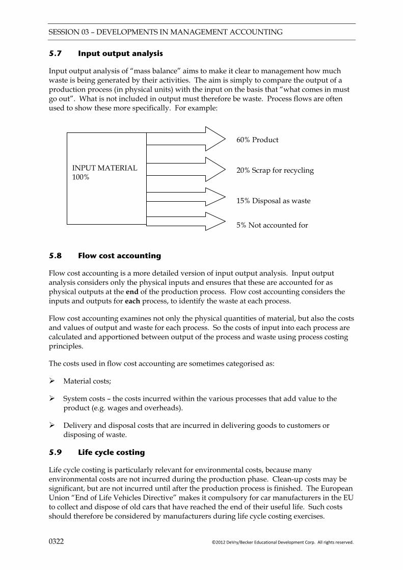
SESSION 03 – DEVELOPMENTS IN MANAGEMENT ACCOUNTING
0322 ©2012 DeVry/Becker Educational Development Corp. All rights reserved.
5.7 Input output analysis
Input output analysis of “mass balance” aims to make it clear to management how much waste is being generated by their activities. The aim is simply to compare the output of a production process (in physical units) with the input on the basis that “what comes in must go out”. What is not included in output must therefore be waste. Process flows are often used to show these more specifically. For example:
5.8 Flow cost accounting
Flow cost accounting is a more detailed version of input output analysis. Input output analysis considers only the physical inputs and ensures that these are accounted for as physical outputs at the end of the production process. Flow cost accounting considers the inputs and outputs for each process, to identify the waste at each process.
Flow cost accounting examines not only the physical quantities of material, but also the costs and values of output and waste for each process. So the costs of input into each process are calculated and apportioned between output of the process and waste using process costing principles.
The costs used in flow cost accounting are sometimes categorised as:
Material costs;
System costs – the costs incurred within the various processes that add value to the product (e.g. wages and overheads).
Delivery and disposal costs that are incurred in delivering goods to customers or disposing of waste.
5.9 Life cycle costing
Life cycle costing is particularly relevant for environmental costs, because many environmental costs are not incurred during the production phase. Clean-up costs may be significant, but are not incurred until after the production process is finished. The European Union “End of Life Vehicles Directive” makes it compulsory for car manufacturers in the EU to collect and dispose of old cars that have reached the end of their useful life. Such costs should therefore be considered by manufacturers during life cycle costing exercises.
INPUT MATERIAL 100%
60% Product
20% Scrap for recycling
15% Disposal as waste
5% Not accounted for
SESSION 03 – DEVELOPMENTS IN MANAGEMENT ACCOUNTING
©2012 DeVry/Becker Educational Development Corp. All rights reserved. 0323
Illustration 6
Xerox Ltd leases photocopying machines to clients. These machines are returned to the company at the end of their lives. One cost that had previously been ignored was the cost of packaging. Xerox would provide packaging for the new machines that were delivered to the customer. The customer would then dispose of this packaging, and have to pay to re pack the old machine that was being returned to Xerox.
As a result of including the costs of packaging in the life cycle costs of the photocopying, the company was able to see how large these costs were. The company now uses a standard re-usable pack. When a machine is delivered to a customer, the package in which it is delivered is used to pack the old machine that is being returned to Xerox. Two standard types of packing have been developed that cover all of Xerox’s machines. This lead to a reduction in packaging costs, and increased customer satisfaction.
Key points
The business environment within which companies operate has become more competitive. Products have shorter life cycles and there is emphasis on quality.
New management accounting techniques have evolved to meet this new environment.
Target costing is used to identify what unit costs would ensure companies make sufficient profit to justify investment. Companies then try to narrow the gap between the actual cost and the target cost by redesigning the product, to “design out” costs.
Life cycle costing involves tracking the cumulative costs and revenues over the life of a product, rather than using the traditional approach to accounting, where costs and revenues are reviewed on a period by period basis. Life cycle costing enables managers to see more clearly how successful a product has been over its whole life.
Throughput accounting is a system which aims to focus management attention onto bottlenecks. Throughput means sales revenue less material cost. Throughput accounting aims to maximise throughput generated per hour by eliminating bottlenecks.
Environmental management accounting aims to provide management with monetary and non-monetary information to enable them to understand and manage the environmental impact of the organisation’s activities.

SESSION 03 – DEVELOPMENTS IN MANAGEMENT ACCOUNTING
0324 ©2012 DeVry/Becker Educational Development Corp. All rights reserved.
FOCUS
You should now be able to:
derive a target cost in manufacturing and service industries;
explain the difficulties of using target costing in service industries;
suggest how a target cost gap might be closed;
identify the costs involved at different stages of the life cycle;
identify the benefits of life cycle costing;
calculate and interpret a throughput accounting ratio (TPAR);
suggest how a TPAR could be improved;
apply throughput accounting to a multi-product decision making problem;
discuss the issues businesses face in the management of environmental costs;
describe the different methods a business may use to account for its environmental costs.
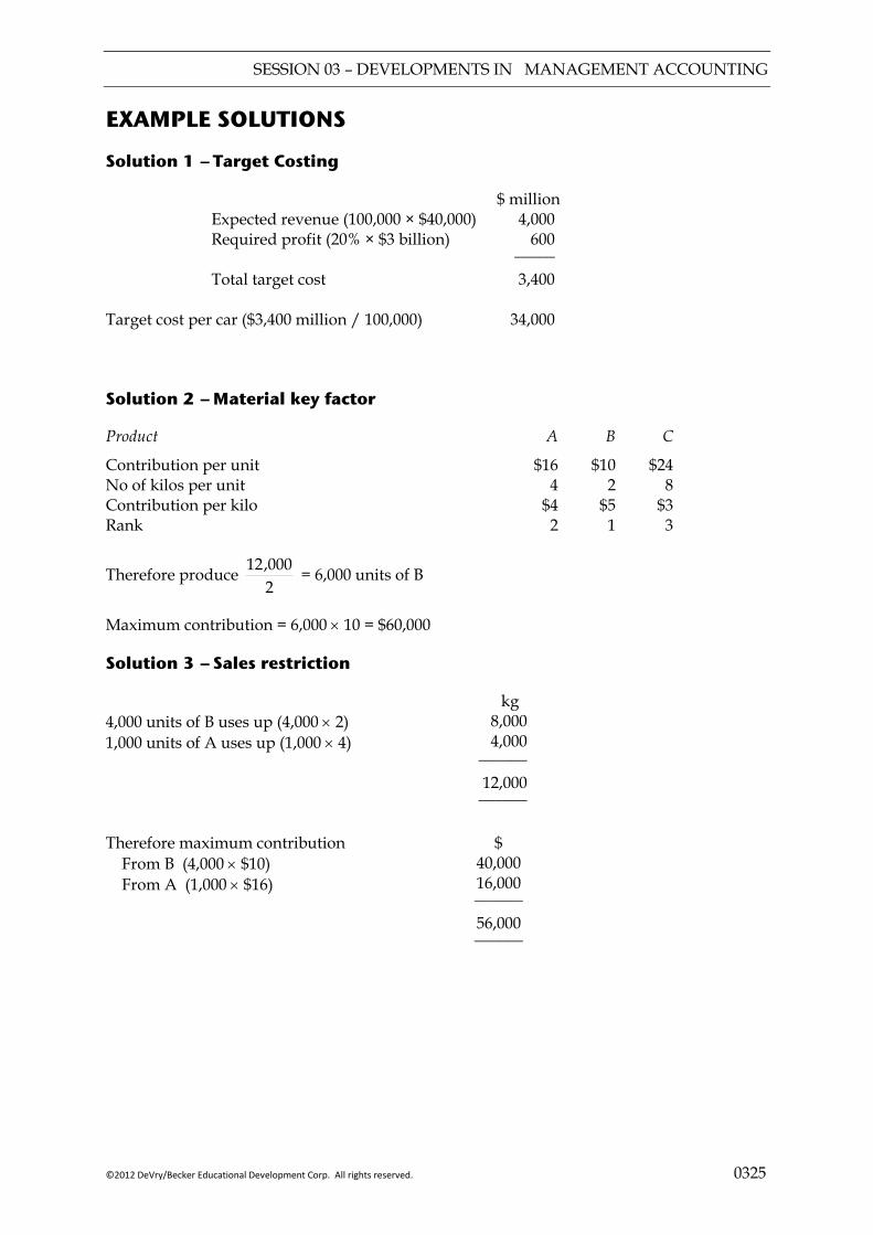
SESSION 03 – DEVELOPMENTS IN MANAGEMENT ACCOUNTING
©2012 DeVry/Becker Educational Development Corp. All rights reserved. 0325
EXAMPLE SOLUTIONS
Solution 1 — Target Costing
$ million Expected revenue (100,000 × $40,000) 4,000 Required profit (20% × $3 billion) 600 _____
Total target cost 3,400 Target cost per car ($3,400 million / 100,000) 34,000
Solution 2 — Material key factor
Product A B C
Contribution per unit No of kilos per unit Contribution per kilo Rank
$16 4
$4 2
$10 2
$5 1
$24 8
$3 3
Therefore produce 2000,12 = 6,000 units of B
Maximum contribution = 6,000 × 10 = $60,000
Solution 3 — Sales restriction
kg 4,000 units of B uses up (4,000 × 2) 1,000 units of A uses up (1,000 × 4)
8,000 4,000
______ 12,000
______ Therefore maximum contribution $ From B (4,000 × $10) From A (1,000 × $16)
40,000 16,000 ______ 56,000 ______
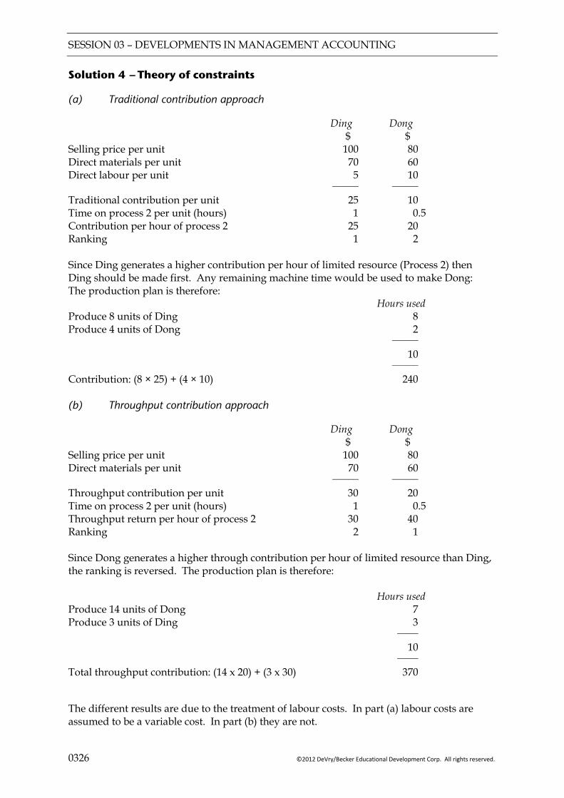
SESSION 03 – DEVELOPMENTS IN MANAGEMENT ACCOUNTING
0326 ©2012 DeVry/Becker Educational Development Corp. All rights reserved.
Solution 4 — Theory of constraints
(a) Traditional contribution approach
Ding Dong $ $ Selling price per unit 100 80 Direct materials per unit 70 60 Direct labour per unit 5 10 _____ _____
Traditional contribution per unit 25 10 Time on process 2 per unit (hours) 1 0.5 Contribution per hour of process 2 25 20 Ranking 1 2 Since Ding generates a higher contribution per hour of limited resource (Process 2) then Ding should be made first. Any remaining machine time would be used to make Dong: The production plan is therefore: Hours used Produce 8 units of Ding 8 Produce 4 units of Dong 2 _____ 10 _____ Contribution: (8 × 25) + (4 × 10) 240 (b) Throughput contribution approach
Ding Dong $ $ Selling price per unit 100 80 Direct materials per unit 70 60 _____ _____
Throughput contribution per unit 30 20 Time on process 2 per unit (hours) 1 0.5 Throughput return per hour of process 2 30 40 Ranking 2 1 Since Dong generates a higher through contribution per hour of limited resource than Ding, the ranking is reversed. The production plan is therefore: Hours used Produce 14 units of Dong 7 Produce 3 units of Ding 3 ____ 10 ____ Total throughput contribution: (14 x 20) + (3 x 30) 370
The different results are due to the treatment of labour costs. In part (a) labour costs are assumed to be a variable cost. In part (b) they are not.
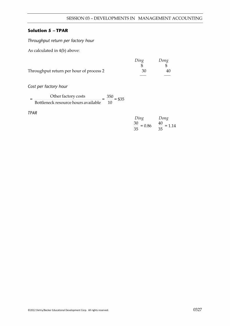
SESSION 03 – DEVELOPMENTS IN MANAGEMENT ACCOUNTING
©2012 DeVry/Becker Educational Development Corp. All rights reserved. 0327
Solution 5 — TPAR
Throughput return per factory hour
As calculated in 4(b) above:
Ding Dong $ $ Throughput return per hour of process 2 30 40 ___ ___ Cost per factory hour
= available hours resource Bottleneck
costs factory Other=
10350 = $35
TPAR Ding Dong
3530 = 0.86
3540 = 1.14

SESSION 03 – DEVELOPMENTS IN MANAGEMENT ACCOUNTING
0328 ©2012 DeVry/Becker Educational Development Corp. All rights reserved.

SESSION 04 – RELEVANT COST ANALYSIS
©2012 DeVry/Becker Educational Development Corp. All rights reserved. 0401
OVERVIEW
Objective
To apply relevant costing principles in short-term decision making.
ONE OFF CONTRACTS
RELEVANT COSTS
OPPORTUNITY COST
SHUT DOWN DECISIONS
Meaning Non-relevant costs
Materials Labour Non-current assets Difficulties in using
opportunity costs
Importance Definition
FURTHER PROCESSING DECISIONS

SESSION 04 – RELEVANT COST ANALYSIS
0402 ©2012 DeVry/Becker Educational Development Corp. All rights reserved.
1 RELEVANT COSTS
1.1 Meaning
“Relevant costs are those costs that are appropriate to aiding the making of specific management decisions.”
Only those costs (and revenues) which will be affected by a decision are “relevant”.
They are:
future;
incremental – i.e. the amount by which costs/revenues will change as a result of the decision;
cash flows – therefore ignore depreciation and gains/ (losses) on disposal, etc.
Avoidable costs – i.e. those which would be avoided if a particular course of action were taken are relevant.
Controllable costs – can be influenced by the actions of the person who controls the budget or cost centre (also called “managed cost”).
1.2 Non-relevant costs
Sunk costs concept – the historic cost of an asset is said to be “sunk” and is irrelevant to any decision.
Commentary However, any realisable value (an incremental, future cash flow) would be relevant – see non-current assets later in this session.
Research and development costs already incurred are similarly “sunk”.
Committed costs (e.g. contract rental and lease payments) are not relevant – although future and cash flows, they are not incremental.
Commentary If a contract is cancellable, such payments are not committed and any penalty costs incurred in cancelling the contract would be relevant.
Fixed costs which are incurred regardless of the decision being taken are irrelevant (but an increment in a fixed cost will be relevant).
Common costs (i.e. allocations and apportionments of shared costs) are subjective (even arbitrary) and not relevant to decisions (e.g. the apportionment of joint costs to joint products).
SESSION 04 – RELEVANT COST ANALYSIS
©2012 DeVry/Becker Educational Development Corp. All rights reserved. 0403
Uncontrollable (“non-controllable”) costs – can be influenced only indirectly by the person in charge of the budget or cost centre. Typically these include “management charges” (i.e. reallocated non-production overheads).
2 OPPORTUNITY COST
2.1 Importance
All opportunity costs are “relevant”.
However, only some relevant costs are opportunity costs.
Commentary The terms “relevant” cost and “opportunity” cost are not synonymous.
2.2 Definition
“The value of the benefit sacrificed when one course of action is chosen, in preference to an alternative. The opportunity cost is represented by the foregone potential benefit from the best rejected course of action.”
For example, the contribution lost if a key worker is moved to a new project is an
opportunity cost relevant to assessing that new project.
Opportunity costs only apply to the use of scarce resources; where resources are not scarce then no sacrifice exists from using these resources.
Illustration 1
A company has been invited to tender for a contract to produce a component, R2D2.
Production of R2D2 will require 100 hours of processing on machine X.
Machine X is working at full capacity producing 50 units of Product Z an hour. Each unit of Product Z makes a contribution of $2.
The lost contribution of $10,000 is an opportunity cost of producing R2D2 and should be taken into account when deciding how much to tender for the contract.
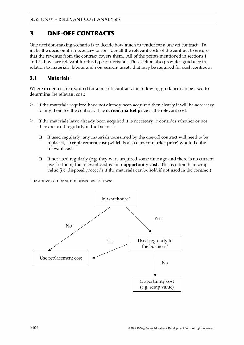
SESSION 04 – RELEVANT COST ANALYSIS
0404 ©2012 DeVry/Becker Educational Development Corp. All rights reserved.
3 ONE-OFF CONTRACTS
One decision-making scenario is to decide how much to tender for a one off contract. To make the decision it is necessary to consider all the relevant costs of the contract to ensure that the revenue from the contract covers them. All of the points mentioned in sections 1 and 2 above are relevant for this type of decision. This section also provides guidance in relation to materials, labour and non-current assets that may be required for such contracts.
3.1 Materials
Where materials are required for a one-off contract, the following guidance can be used to determine the relevant cost:
If the materials required have not already been acquired then clearly it will be necessary to buy them for the contract. The current market price is the relevant cost.
If the materials have already been acquired it is necessary to consider whether or not they are used regularly in the business:
If used regularly, any materials consumed by the one-off contract will need to be replaced, so replacement cost (which is also current market price) would be the relevant cost.
If not used regularly (e.g. they were acquired some time ago and there is no current use for them) the relevant cost is their opportunity cost. This is often their scrap value (i.e. disposal proceeds if the materials can be sold if not used in the contract).
The above can be summarised as follows:
In warehouse?
No
Use replacement cost
Used regularly in the business?
Yes
Yes
No
Opportunity cost (e.g. scrap value)

SESSION 04 – RELEVANT COST ANALYSIS
©2012 DeVry/Becker Educational Development Corp. All rights reserved. 0405
Key points
Historic costs or book values are never relevant costs of materials.
Commentary Examiners may provide a lot of superfluous information, such as “the auditors have demanded that the value of materials be written down to their net realisable value”, which is completely irrelevant.
3.2 Labour
One-off contracts will usually require some labour. The relevant cost of labour can be determined from the following situations:
If the organisation has spare (idle) labour time which can be used on the contract, then the relevant cost is zero. This might arise for example where workers are being paid a fixed weekly wage and are currently under-employed.
If additional labour time is required and this can be obtained without taking workers away from other activities, then the direct cost of the labour is relevant. This may be paid at a higher rate if overtime is involved.
If there is a limit on the amount of labour available a contract may require workers to be taken away from other profitable activities. In this case the relevant cost of labour is the direct cost plus the lost contribution from the other activities. (Learn this as a rule but see Example 2 in Session 6 for further explanation.)
3.3 Non-current assets
Where a contract requires the use of a machine or other non-current asset, then the deprival value is the relevant cost. This measures the value to a business of an existing asset in terms of the cost incurred if the business were to be deprived of it (in other words, if the machine is used on a one off contract, it would not be available for “normal activities”.
Deprival value is calculated as follows:
RC = Replacement cost NRV = Net realisable value EV = Economic value (i.e. the PV of expected future earnings which the asset will generate
The lower of
RC and The higher of
NRV EV
SESSION 04 – RELEVANT COST ANALYSIS
0406 ©2012 DeVry/Becker Educational Development Corp. All rights reserved.
Commentary This is easily remembered as a two-stage decision: Decision 1 – should the asset be kept in use in the business or sold? (For assets in use EV should be higher than NRV.) Decision 2 – if deprived of the asset (e.g. through sale or use elsewhere) will it be replaced?
Illustration 2
An asset which will be transferred to a new contract, if it is undertaken, has:
Replacement cost $200,000 Net realisable value $50,000 Economic value $100,000
The opportunity cost of the asset is $100,000.
Example 1
Identify the deprival value in each for the following cases:
Case RC NRV EV
1 500 600 550
2 700 600 550
3 700 600 650
Solution
1
2
3

SESSION 04 – RELEVANT COST ANALYSIS
©2012 DeVry/Becker Educational Development Corp. All rights reserved. 0407
Example 2
Stella is about to tender for a contract which requires the use of two raw materials, steel and tungsten. 500 tons of steel and 1,000 tons of tungsten will be required to complete the contract. In addition 2,000 hours of labour will be needed. Of this, 1,200 hours are in the assembly process and the remainder in the finishing process. Stella will quote a price that allows a 50% mark-up on relevant cost.
The following additional information is available for the resources required:
In inventory Original price Current price Net realisable now per ton per ton value Steel 200 tons $10 $12 $8 Tungsten 400 tons $20 $23 $15 Steel cannot be used by Stella for any other purpose, but tungsten is used in all the company’s manufacturing processes.
All labour is paid $4 per hour, but to complete the contract in time, labour for the finishing process will have to be transferred from other work which generates contribution at a rate of $3 per hour (after labour costs). There is currently surplus capacity for assembly labour amounting to 1,000 hours for the duration of the contract. Owing to other urgent work any additional assembly labour will have to be hired on a temporary basis at the rate of $5 per hour.
Required:
Determine the price Stella will quote on the contract.
SESSION 04 – RELEVANT COST ANALYSIS
0408 ©2012 DeVry/Becker Educational Development Corp. All rights reserved.
Solution
WORKING $ Steel:
Held
Purchased
Tungsten:
Finishing labour:
Cost
Lost contribution
Assembly labour:
______
Relevant cost
Mark-up
______
Quote
______
3.4 Difficulties in using opportunity costs
Estimating future costs/revenues and hence the benefit sacrificed.
Identifying alternative uses and hence the best alternative forgone.
Ignores effect on accounting profit.
Ignores the risk of each alternative.
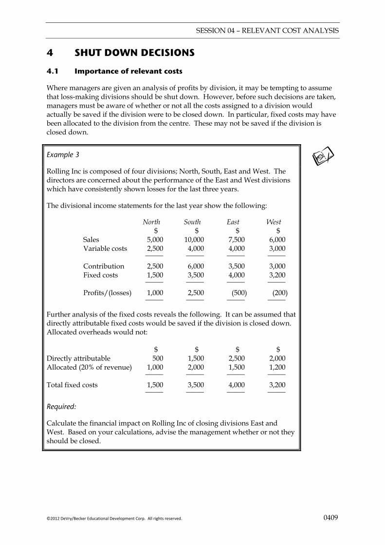
SESSION 04 – RELEVANT COST ANALYSIS
©2012 DeVry/Becker Educational Development Corp. All rights reserved. 0409
4 SHUT DOWN DECISIONS
4.1 Importance of relevant costs
Where managers are given an analysis of profits by division, it may be tempting to assume that loss-making divisions should be shut down. However, before such decisions are taken, managers must be aware of whether or not all the costs assigned to a division would actually be saved if the division were to be closed down. In particular, fixed costs may have been allocated to the division from the centre. These may not be saved if the division is closed down.
Example 3
Rolling Inc is composed of four divisions; North, South, East and West. The directors are concerned about the performance of the East and West divisions which have consistently shown losses for the last three years.
The divisional income statements for the last year show the following:
North South East West $ $ $ $ Sales 5,000 10,000 7,500 6,000 Variable costs 2,500 4,000 4,000 3,000 _____ _____ _____ _____
Contribution 2,500 6,000 3,500 3,000 Fixed costs 1,500 3,500 4,000 3,200 _____ _____ _____ _____
Profits/(losses) 1,000 2,500 (500) (200) _____ _____ _____ _____
Further analysis of the fixed costs reveals the following. It can be assumed that directly attributable fixed costs would be saved if the division is closed down. Allocated overheads would not: $ $ $ $ Directly attributable 500 1,500 2,500 2,000 Allocated (20% of revenue) 1,000 2,000 1,500 1,200 _____ _____ _____ _____
Total fixed costs 1,500 3,500 4,000 3,200 _____ _____ _____ _____
Required:
Calculate the financial impact on Rolling Inc of closing divisions East and West. Based on your calculations, advise the management whether or not they should be closed.
SESSION 04 – RELEVANT COST ANALYSIS
0410 ©2012 DeVry/Becker Educational Development Corp. All rights reserved.
Solution
East West $ $
_____ _____
Net savings/(losses)
_____ _____
Conclusion:
5 FURTHER PROCESSING DECISIONS
5.1 Joint-product situations
These types of decision are based on situations where several products are produced by a process. It may be possible to increase the value of some of the products if they are further processed. The approach is therefore to look at the additional revenue that would be gained if further processing takes place, and deduct from this the costs of further processing.
Illustration 3
Two products G and H are created from a joint process. G can be sold immediately after split-off. H requires further processing before it is in a saleable condition. There are no opening stocks and no work in progress. The following data are available for last period:
$ Total joint production costs 384,000 Further processing costs (product H) 159,600 Product Selling price per unit G $0·84 (400,000) H $1·82 (200,000 units) The relevant costs and revenues in determining whether H should be processed further are the additional revenue of $364,000 less the costs of further processing of $159,600. Further processing of H increases profits by $204,400, so H should be further processed.

SESSION 04 – RELEVANT COST ANALYSIS
©2012 DeVry/Becker Educational Development Corp. All rights reserved. 0411
Key points
In decision making, the relevant costs and revenues are those that change as a result of the decision. All other revenues and costs should be ignored.
Opportunity costs should be taken into consideration, as these are a relevant to the decision.
Decision-making scenarios include “one off contracts” where the relevant cost of performing a contract is calculated.
Shut down decisions involve the decision to close a loss making division. In making such decisions, it should be recognised that some of the costs of the loss making division may not be saved if the division is closed, so are not therefore relevant to the decision.
Further processing decisions involve whether it is worthwhile processing joint or by products further.
FOCUS
You should now be able to:
explain the concept of relevant costing;
identify and calculate relevant costs for a specific decision situation from given data;
explain and apply the concept of opportunity cost;
apply relevant costing principles in situations involving shut down, one off contracts and the further processing of joint products.

SESSION 04 – RELEVANT COST ANALYSIS
0412 ©2012 DeVry/Becker Educational Development Corp. All rights reserved.
EXAMPLE SOLUTIONS
Solution 1 — Deprival value
Case RC NRV PV 1 500 600 550 2 700 600 550 3 700 600 650
Solution 2 — Relevant costs
WORKING $ Steel Held (NRV) 200 tons @ $8 1,600
Purchased 300 tons @ $12 3,600
Tungsten 1,000 tons @ 23 23,000
Finishing labour – Cost 800 hours @ $4 3,200
– Lost contribution 800 hours @ $3 2,400
Assembly labour 200 hours @ $5 1,000 ______ Relevant cost 34,800 Mark-up 17,400 ______ Quote 52,200 ______ Solution 3 — Shut down decisions
East West $ $ Lost contribution (3,500) (3,000) Saved fixed costs (attributable only) 2,500 2,000 _____ _____
Net savings/(losses) (1,000) (1,000) _____ _____
Conclusion
Closing each division would lead to a reduction in profits of $1,000 per year. They should not be closed. The two departments make a positive contribution to the company’s overall profits and only show a loss because of allocation of central fixed costs.

SESSION 05 – CVP ANALYSIS
©2012 DeVry/Becker Educational Development Corp. All rights reserved. 0501
OVERVIEW
Objective
To understand the concept of breakeven and margin of safety and carry out CVP analysis.
BREAKEVEN ANALYSIS
MATHEMATICAL APPROACH CHARTS
Breakeven point Simplifying assumptions
Breakeven chart Profit-volume chart
Contribution Breakeven formulae C/S ratio Margin of safety
MULTI-PRODUCT ANALYSIS
Assumption Calculation
Simplifying assumptions Multi product situations
LIMITATIONS IN PLANNING AND
DECISION MAKING

SESSION 05 – CVP ANALYSIS
0502 ©2012 DeVry/Becker Educational Development Corp. All rights reserved.
1 BREAKEVEN ANALYSIS
Definition
Breakeven point is the level of activity at which neither a profit nor a loss is made.
Commentary That is, where total contribution = total fixed costs.
It indicates the lowest activity level at which the activity is viable. (It may be regarded as a “life and death” measure.)
It is ascertained by a breakeven chart or calculation.
1.1 Simplifying assumptions
Within the range of activity under consideration total cost behaves as a strictly linear semi-variable cost:
Fixed costs remain fixed over; Total variable costs change proportionally with volume.
Unit selling prices do not change with volume.
Costs and income are matched (i.e. there is no significant change in inventory levels).
Levels of efficiency and productivity do not change (as this would affect cost behaviour).
There is only a single product or a constant sales mix of more than one product.
Total costs and total revenue are linear functions of output.
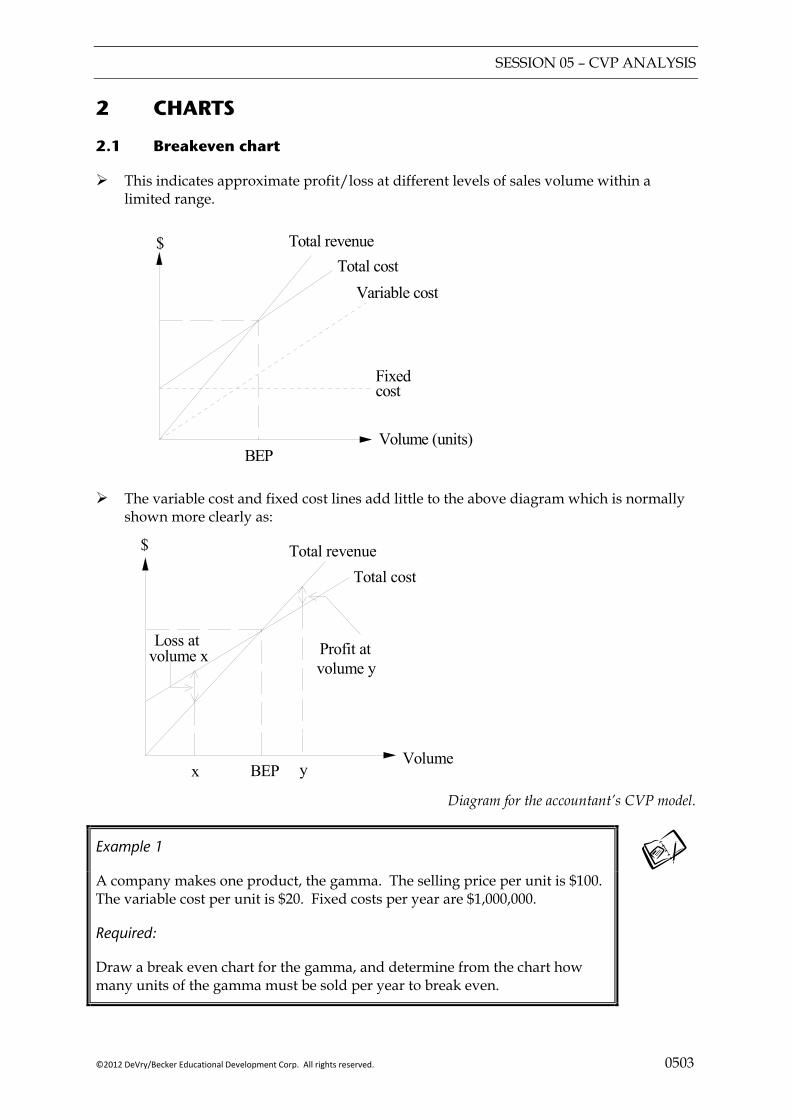
SESSION 05 – CVP ANALYSIS
©2012 DeVry/Becker Educational Development Corp. All rights reserved. 0503
2 CHARTS
2.1 Breakeven chart
This indicates approximate profit/loss at different levels of sales volume within a limited range.
$ Total revenueTotal cost
Variable cost
Fixed
Volume (units)
cost
BEP
The variable cost and fixed cost lines add little to the above diagram which is normally shown more clearly as:
$ Total revenueTotal cost
Profit atvolume y
Loss atvolume x
x BEP yVolume
Diagram for the accountant’s CVP model.
Example 1
A company makes one product, the gamma. The selling price per unit is $100. The variable cost per unit is $20. Fixed costs per year are $1,000,000.
Required:
Draw a break even chart for the gamma, and determine from the chart how many units of the gamma must be sold per year to break even.

SESSION 05 – CVP ANALYSIS
0504 ©2012 DeVry/Becker Educational Development Corp. All rights reserved.
Solution
2.2 Profit-volume chart
A “PV” chart is another way of presenting the same information as a breakeven chart but it emphasises profits and losses at different activity levels (i.e. sales volume or value).
To draw it requires only the following information:
profit/(loss) at any (i.e. just one) level of sales; and total fixed costs.
Profit
VolumeBEP
x y
Profit atvolume y
0
Loss atvolume x
$
Fixedcosts
Commentary At zero sales volume, total loss is the amount of the fixed costs.
$000
Sales (units)
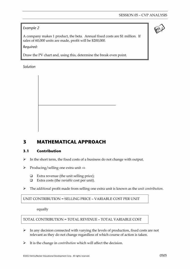
SESSION 05 – CVP ANALYSIS
©2012 DeVry/Becker Educational Development Corp. All rights reserved. 0505
Example 2
A company makes 1 product, the beta. Annual fixed costs are $1 million. If sales of 60,000 units are made, profit will be $200,000.
Required:
Draw the PV chart and, using this, determine the break even point.
Solution
3 MATHEMATICAL APPROACH
3.1 Contribution
In the short term, the fixed costs of a business do not change with output.
Producing/selling one extra unit ⇒
Extra revenue (the unit selling price); Extra costs (the variable cost per unit).
The additional profit made from selling one extra unit is known as the unit contribution.
UNIT CONTRIBUTION = SELLING PRICE – VARIABLE COST PER UNIT
equally
TOTAL CONTRIBUTION = TOTAL REVENUE – TOTAL VARIABLE COST
In any decision connected with varying the levels of production, fixed costs are not
relevant as they do not change regardless of which course of action is taken.
It is the change in contribution which will affect the decision.
SESSION 05 – CVP ANALYSIS
0506 ©2012 DeVry/Becker Educational Development Corp. All rights reserved.
3.2 Breakeven formulae
3.2.1 BEP
Profit = Sales – Variable cost – Fixed cost = Total contribution – Fixed cost
At BEP, profit = 0 Therefore Total contribution = Fixed cost
But, Total contribution = Number of units × Unit contribution
Therefore, Number of units to be sold to breakeven
oncontributi Unitcost fixed Total
=
3.2.2 Target profits
Sales volume to achieve a target profit
oncontributi Unitprofit required + cost Fixed
=
Sales revenue to achieve a target profit = × unit selling price
3.2.3 Break even revenue
BEP is expressed in terms of the number of units that must be sold in order to break even.
Break even revenue is the revenue that is achieved at the BEP. One way of calculating this is simply to multiply the selling price per unit times the number of units at BEP.
Example 3
Using the information in Example 1 calculate:
(a) the break even point for the gamma using the numerical approach; (b) the sales volume required to make a profit of $100,000; (c) the revenue at break even point.
Solution

SESSION 05 – CVP ANALYSIS
©2012 DeVry/Becker Educational Development Corp. All rights reserved. 0507
3.3 C/S ratio
Commentary Although this is also called the profit/volume (or P/V) ratio this is a misnomer. As profit is not the same as contribution and volume is not the same as sales.
3.3.1 C/S Ratio
Contribution/sales ratio (also called “contribution margin”) is the proportion of selling price which contributes to fixed overheads and profits.
unit per priceSelling unit peron Contributi
=
revenue sales Totaloncontributi Total or
3.3.2 Breakeven revenue
The C/S ratio can be used as an alternative way of calculating break even revenue, without calculating break even point.
Break even revenue ratio C/S
cost Fixed=
Revenue required to achieve a target profit ratio C/S
profit required + cost Fixed=
Example 4
Using the information in Example 1, calculate:
(a) the C/S ratio for the gamma; and
(b) the break even revenue using the C/S ratio.
Solution
SESSION 05 – CVP ANALYSIS
0508 ©2012 DeVry/Becker Educational Development Corp. All rights reserved.
3.4 Margin of safety
Definition
The amount by which anticipated or existing activity exceeds (or falls short of) breakeven.
In units or $s Margin of safety = Budgeted sales – Breakeven sales
As a percentage %100
sales BudgetedsalesBreakeven -sales Budgeted
×
Example 5
Continuing on from Examples 3 and 4, the company expects to sell 20,000 units of the gamma per year.
Required:
Calculate the margin of safety in terms of number of units, and as a percentage.
Solution
In units
As a percentage
Example 6
A company manufactures a single product which has the following cost structure based on a production budget of 10,000 units. $ Materials – 4 kg at $3/kg 12 Direct labour – 5 hours at $7/hour 35
Variable production overheads are recovered at the rate of $8 per direct labour hour. Other costs incurred by the company are: $ Factory fixed overheads 120,000 Selling and distribution overheads 160,000 Fixed administration overheads 80,000
The selling and distribution overheads include a variable element due to a distribution cost of $2 per unit. The fixed selling price of the unit is $129.
Required:
(a) Calculate how many units have to be sold for the company to breakeven. (b) Calculate the sales revenue which would give a net profit of $40,000.
SESSION 05 – CVP ANALYSIS
©2012 DeVry/Becker Educational Development Corp. All rights reserved. 0509
Solution
(a) Break even number of units $ Materials
Labour
Variable overheads
Distribution
_____
Total variable cost
Selling price
_____
Unit contribution
_____
Fixed costs $
Factory
Selling and distribution (after excluding variable element)
Administration _______ Total fixed cost _______
BEP =
(b) Sales revenue ⇒ Target profit $40,000 $ Total fixed costs
Profit required _______ Total contribution required _______
oncontributi Unitoncontributi Total =
Total revenue required:
SESSION 05 – CVP ANALYSIS
0510 ©2012 DeVry/Becker Educational Development Corp. All rights reserved.
4 MULTI-PRODUCT ANALYSIS
4.1 Assumption
CVP analysis can be extended to multi-product situations if a pre-determined sales mix is held to be constant.
If the assumption of standard mix is relaxed, there will be no unique BEP.
4.2 Calculation of break even point
Define a standard “basket” (or “batch”) of products, based on the expected sales mix (e.g. if expected sales volume of product A is twice that of Product B, then one basket is defined as “2 units of product A and 1 units of product B”).
Calculate the contribution per basket.
Use break even formulae as for single-product analysis to calculate the number of baskets that would need to be sold to achieve break even:
Break even point basket peron Contributi oncontributi Total
Having calculated the number of baskets that must be sold to achieve break even or target profits, convert back to number of units of each product by multiplying the number of baskets by the unit of each product in one batch.
Example 7
Pear manufactures laptop computers and smart phones. The company has prepared the following forecast for the following financial period:
Lap tops Smart phones Budgeted sales 1200 600 $ $ Unit selling price 1,000 500 Unit variable cost 700 400 _____ _____
Unit contribution 300 100 _____ _____
Budgeted fixed costs are $245,000 for the period.
Required:
Assuming that the sales mix will always be 2 laptops to 1 smart phone, calculate:
(a) The break even point expressed in terms of units of each product.
(b) The margin of safety in percentage terms, based on budgeted sales.

SESSION 05 – CVP ANALYSIS
©2012 DeVry/Becker Educational Development Corp. All rights reserved. 0511
Solution
A “basket” is
Contribution of a basket is
(a) Break even point
In baskets:
In units:
(b) Margin of safety
4.3 C/S Ratio in multi-product situations
4.3.1 Calculation
As described above, the C/S ratio in single product situations:
unit per priceSelling unit peron Contributi
=
revenue sales Totaloncontributi Total or
In multi-product situations, a weighted average C/S ratio can easily be found taking total contribution divided by total sales revenue.
4.3.2 Meaning
The C/S ratio specifies how much contribution will be generated by an increase in sales revenue of $1. In multi-product situations, sales mix is assumed to remain constant.
4.3.3 Uses
The C/S ratio can be used to find the following:
Break even revenue; Sales revenue required to generate a target profit.
There is nothing new here – simply apply the same formulae used above in single-product situations to a multi-product situation:
Break even revenue ratio C/S average Weighted
cost Fixed=
Revenue required to achieve a target profit ratio C/S average Weighted
profit required + cost Fixed=

SESSION 05 – CVP ANALYSIS
0512 ©2012 DeVry/Becker Educational Development Corp. All rights reserved.
Example 8
Required:
Using the date in Example 7 calculate:
(a) The break even revenue, using the weighted average C/S ratio; (b) The sales revenue required to make a target profit of $245,000.
Solution
WORKINGS
(a) Break even revenue
(b) Sales revenue to make a profit of $245,000
4.4 Multi-product P/V graphs
In a multi-product environment, sales revenue is drawn on the horizontal axis (x axis), and profit on the vertical axis (y axis). Two approaches are taken to drawing the line denoting profit/loss:
constant (fixed) sales mix; ranking of products by profitability.
4.4.1 Assuming a constant sales mix
Assuming a constant mix of products based on the budgeted sales it is only necessary to know profit for two values of sales (to plot on the graph and draw a straight line between them):
The easiest point is where revenue = 0 (i.e. where the company makes a loss equal to fixed costs;
For the second point it makes most sense to calculate profit for budgeted sales.
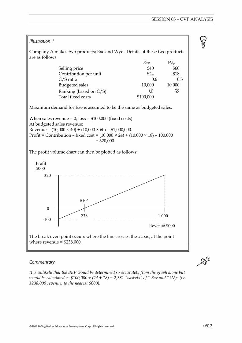
SESSION 05 – CVP ANALYSIS
©2012 DeVry/Becker Educational Development Corp. All rights reserved. 0513
Illustration 1
Company A makes two products; Exe and Wye. Details of these two products are as follows: Exe Wye Selling price $40 $60 Contribution per unit $24 $18 C/S ratio 0.6 0.3 Budgeted sales 10,000 10,000 Ranking (based on C/S) Total fixed costs $100,000
Maximum demand for Exe is assumed to be the same as budgeted sales. When sales revenue = 0; loss = $100,000 (fixed costs) At budgeted sales revenue: Revenue = (10,000 × 40) + (10,000 × 60) = $1,000,000. Profit = Contribution – fixed cost = (10,000 × 24) + (10,000 × 18) – 100,000 = 320,000. The profit volume chart can then be plotted as follows:
The break even point occurs where the line crosses the x axis, at the point where revenue = $238,000.
Commentary It is unlikely that the BEP would be determined so accurately from the graph alone but would be calculated as $100,000 ÷ (24 + 18) = 2,381 “baskets” of 1 Exe and 1 Wye (i.e. $238,000 revenue, to the nearest $000).
Revenue $000
1,000
Profit $000
-100
0
320
BEP
238

SESSION 05 – CVP ANALYSIS
0514 ©2012 DeVry/Becker Educational Development Corp. All rights reserved.
4.4.2 Assuming sales by “profitability”
An alternative assumption is that sales are not made in a standard sales mix but by profitability of product (i.e. the company produces and sells the product with the highest contribution first). Products are therefore ranked according to the C/S ratios.
In this case, the PV chart will no longer be a straight line; it will be “kinked”. To draw the graph, it is advisable to do a table first, calculating profit at the following points:
(1) Sales revenue = 0 (2) Maximum sales of the most profitable product, with no sales of the second product. (3) Maximum sales of the first and second products. (4) Maximum sales of the first, second and third products (if there are three products). And so on.
Illustration 3
Continuing from Illustration 2, assume now that company A decides to produce and sell product Exe first, as this has the highest C/S ratio, followed by product Wye. The calculation of profits at the key points is as follows:
Contribution Cumulative Revenue Cumulative Profit/(loss) Revenue Sales revenue = 0 0 (100,000) 0 0 Max sales of Exe 240,000 140,000 400,000 400,000 Max sales of Wye 180,000 320,000 600,000 1,000,000 Drawing the line joining these key points gives the CVP graph:
Up to revenue of $240,000 the company is selling only Exe. After this it starts to sell Wye. Since Wye generates contribution at a lower rate per $ of revenue than Exe, the line is more flat after this point. The break even point is where the line crosses the x axis, at the point where sales = $166,000. This is lower than the break even point assuming a constant sales mix (Illustration 1). This is because the C/S ratio of product Exe is higher than the weighted average C/S ratio of the two products together.
Revenue $000
1,000
Profit $000
-100
0
320
Break even point
240
140
166
SESSION 05 – CVP ANALYSIS
©2012 DeVry/Becker Educational Development Corp. All rights reserved. 0515
Example 9
Plum manufactures two types of car; the “boy racer” and the “family saloon”. The following budgeted daily information has been prepared:
Boy racer Family saloon Budgeted sales 300 600 $ $ Unit selling price 10,000 15,000 Unit variable cost 5,000 12,000 _____ _____
Unit contribution 5,000 3,000 _____ _____
Budgeted fixed costs are $1 million per day.
Required:
Assuming that the budgeted sales represents maximum sales of each of the two products, draw the CVP chart for the two products based on the assumption that:
(a) Sales occur in the standard (budgeted) mix; and (b) Sales of the most profitable product occur first, followed by sales of the
second product.
Draw both lines on one graph.
Solution

SESSION 05 – CVP ANALYSIS
0516 ©2012 DeVry/Becker Educational Development Corp. All rights reserved.
5 LIMITATIONS IN PLANNING AND DECISION MAKING
5.1 Simplifying assumptions
The main limitations of CVP analysis for planning and decision making relate to the assumptions that have to be made. In summary, these are:
Fixed costs remain constant regardless of the production decision. In practice fixed costs may not be truly fixed and may vary as output changes.
Variable cost per unit is constant (which may not be the case due to discounts and other economies of scale).
Selling price remains constant. This may not be true in practice, where an increase in volume of sales can only be achieved by lowering the price.
5.2 Multi product situations
It is necessary to assume a fixed product mix to work with multi product situations. If the product mix is allowed to vary, there could potentially be many break even points. In practice companies would want to know how varying their product mix will affect profits.
Key points
Break even point is the point at which a company makes a profit of zero. To break even a company needs to sell enough units to cover its fixed and variable costs.
It is common in exams to see a break even chart which shows how total costs and total revenues vary with output. Another type of chart is the PV (Profit-Volume) chart, which shows how profit varies with output.
The following formulae are all easily derived and are not provided in the examination:
Break even point oncontributi Unit
cost fixed Total=
C/S ratio unit per priceSelling unit peron Contributi
=
Break even revenue ratio C/S
cost Fixed=
In multi-product situations, a standard product mix is assumed. The same calculations can then be done as for a single product case, by defining a standard “batch” or “basket” of the products.
The usefulness of CVP analysis is limited by the assumptions that have to be made to make it workable.

SESSION 05 – CVP ANALYSIS
©2012 DeVry/Becker Educational Development Corp. All rights reserved. 0517
FOCUS
You should now be able to:
explain the nature of CVP analysis;
calculate and interpret break even point and margin of safety;
calculate the contribution to sales ratio, in single and multi-product situations and demonstrate an understanding of its use;
prepare break even charts and profit volume charts and interpret the information contained within each, including multi-product situations;
discuss the limitations of CVP analysis for planning and decision making.

SESSION 05 – CVP ANALYSIS
0518 ©2012 DeVry/Becker Educational Development Corp. All rights reserved.
EXAMPLE SOLUTIONS
Solution 1 — Break Even Chart
From the diagram below, it can be seen that the break even level of sales is 12,500 units.
$000
1,000
1,500
Sales (units) 15,00012,500
1,300
Total revenue
Total costs
Commentary In order to draw each line, it is necessary to calculate total cost or total revenue at two levels of output, and draw a straight line between them:
Total revenue
When output is 0, total revenue is zero. An output level of 15,000 units was chosen at random. At an output level of 15,000 units, total revenue would be $15 million ($100 per unit × 15,000 units.)
Total costs
When output = 0, total costs = fixed costs, = $1 million.
At output level of 15,000 units (chosen at random) total variable costs are $300,000 ($20 per unit × 15,000). Fixed costs are $1 million. Therefore total costs are $1,300,000.
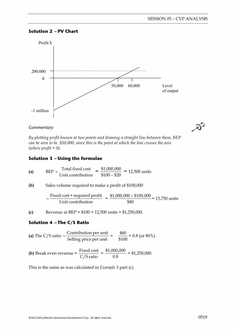
SESSION 05 – CVP ANALYSIS
©2012 DeVry/Becker Educational Development Corp. All rights reserved. 0519
Solution 2 — PV Chart
Commentary By plotting profit known at two points and drawing a straight line between them, BEP can be seen to be $50,000, since this is the point at which the line crosses the axis (where profit = 0).
Solution 3 — Using the formulae
(a) BEP oncontributi Unit
cost fixed Total= =
20$100$000,000,1$
− = 12,500 units
(b) Sales volume required to make a profit of $100,000
oncontributi Unit
profit required + cost Fixed= =
80$000,100$000,000,1$ + = 13,750 units
(c) Revenue at BEP = $100 × 12,500 units = $1,250,000.
Solution 4 — The C/S Ratio
(a) The C/S ratio unit per priceSelling unit peron Contributi
= = 100$80$ = 0.8 (or 80%).
(b) Break even revenue = ratio C/Scost Fixed =
8.0000,000,1$ = $1,250,000.
This is the same as was calculated in Example 3 part (c).
Level of output
60,000
Profit $
200,000
-1 million
50,000
0

SESSION 05 – CVP ANALYSIS
0520 ©2012 DeVry/Becker Educational Development Corp. All rights reserved.
Solution 5 — Margin of Safety
In units Margin of safety = Budgeted sales – Breakeven sales
= 20,000 – 12,500 = 7,500 units.
As a percentage %100
sales BudgetedsalesBreakeven -sales Budgeted
×
00020
5001200020,
,, − × 100% = 37.5%.
This means that sales can fall by 37.5% before the company will no longer make a profit.
Solution 6 — More complex example
(a) Break even number of units $ Materials 12 Labour 35 Variable overheads 40 Distribution 2 ____
Total variable cost 89 Selling price 129
Unit contribution
____
40 ____
$ Factory 120,000 Selling and distribution
(after excluding variable element)
140,000 Administration 80,000
Total fixed cost
_______
340,000 _______
BEP = units 500,840
000,340oncontributi Unit
costs fixed Total==
(b) Sales revenue ⇒ Target profit $40,000 $ Total fixed costs 340,000 Profit required 40,000
Total contribution required
_______
380,000 _______
units 9,500 40
000,380oncontributi Unitoncontributi Total
==
Total revenue required: 9,500 × $129 = $1,225,500
SESSION 05 – CVP ANALYSIS
©2012 DeVry/Becker Educational Development Corp. All rights reserved. 0521
Solution 7 — Multi product break even point
A “basket” consists of 2 laptops and 1 smart phone. The contribution generated by a basket is $700 (2 × 300 +1×100)
(a) Break even point
Using the standard formula, BEP = baskets 350 700
000245oncontributi Unitoncontributi Total
==,
350 baskets equates to 700 laptops and 350 smart phones.
(b) Margin of safety
Working in baskets, budgeted sales equates to 600 baskets. Break even sales = 350 baskets.
Margin of safety = %100sales Budgeted
salesBreakeven -sales Budgeted× = %100
600350 -600
× = 41.47%.
Solution 8 — Using C/S ratio in a multi-product situation
The weighted average C/S ratio is sales (budgeted) Total
oncontributi (budgeted) Total
Total budgeted contribution is (1,200 × 300) + (600 × 100) = $420,000
Total budgeted revenue is (1,200 × 1,000) + (600 × 500) = $1,500,000
Weighted average C/S ratio is therefore 1,500,000420,000 = 0.28
(a) Break even revenue
ratio C/S average Weighted cost Fixed
= = 280000245
., = $875,000.
(b) Sales revenue to make a profit of $245,000
ratio C/S average Weightedprofit required + cost Fixed
= = 280
000245000245.
,, + $1,750,000
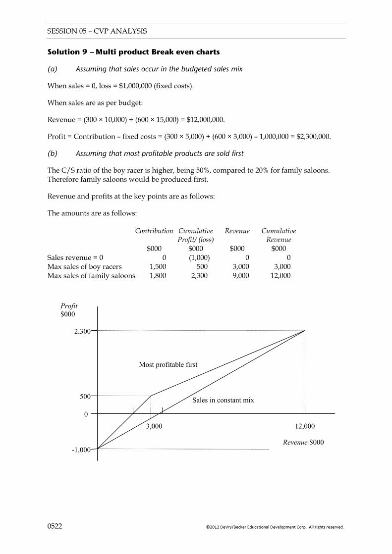
SESSION 05 – CVP ANALYSIS
0522 ©2012 DeVry/Becker Educational Development Corp. All rights reserved.
Solution 9 — Multi product Break even charts
(a) Assuming that sales occur in the budgeted sales mix
When sales = 0, loss = $1,000,000 (fixed costs).
When sales are as per budget:
Revenue = (300 × 10,000) + (600 × 15,000) = $12,000,000.
Profit = Contribution – fixed costs = (300 × 5,000) + (600 × 3,000) – 1,000,000 = $2,300,000.
(b) Assuming that most profitable products are sold first
The C/S ratio of the boy racer is higher, being 50%, compared to 20% for family saloons. Therefore family saloons would be produced first.
Revenue and profits at the key points are as follows:
The amounts are as follows: Contribution Cumulative Revenue Cumulative Profit/ (loss) Revenue $000 $000 $000 $000 Sales revenue = 0 0 (1,000) 0 0 Max sales of boy racers 1,500 500 3,000 3,000 Max sales of family saloons 1,800 2,300 9,000 12,000
Revenue $000
3,000
Profit $000
-1,000
0
2,300
500
12,000
Most profitable first
Sales in constant mix
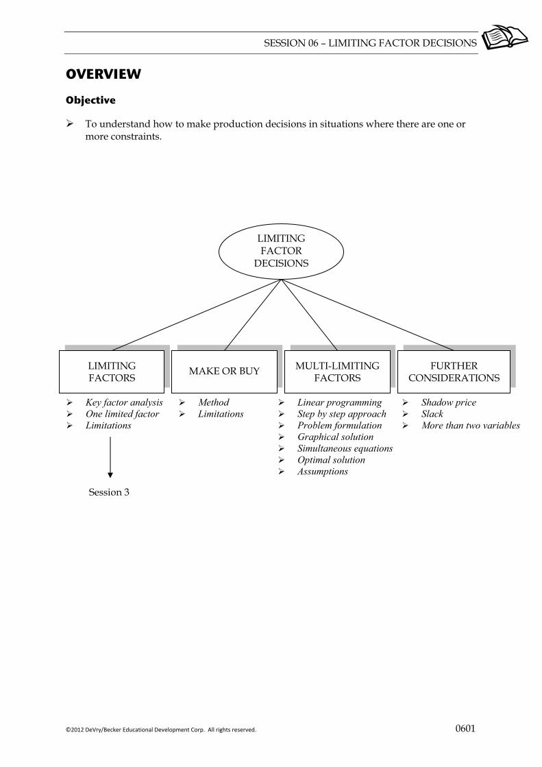
SESSION 06 – LIMITING FACTOR DECISIONS
©2012 DeVry/Becker Educational Development Corp. All rights reserved. 0601
OVERVIEW
Objective
To understand how to make production decisions in situations where there are one or more constraints.
LIMITING FACTORS
FURTHER CONSIDERATIONS
MULTI-LIMITING FACTORS
Key factor analysis One limited factor Limitations
MAKE OR BUY
Method Limitations
Linear programming Step by step approach Problem formulation Graphical solution Simultaneous equations Optimal solution Assumptions
Shadow price Slack More than two variables
LIMITING FACTOR
DECISIONS
Session 3
SESSION 06 – LIMITING FACTOR DECISIONS
0602 ©2012 DeVry/Becker Educational Development Corp. All rights reserved.
1 LIMITING FACTORS
1.1 Key factor analysis
In the short term, sales demand may be greater than productive capacity. For example, output may be limited by a shortage of factors such as:
labour; materials; machinery; floor space.
Where limiting factors apply, profit is maximised by maximising contribution. Contribution is sales revenue minus variable costs. Maximising contribution automatically maximises profit, because profit is equal to contribution minus fixed costs.
1.2 One limited factor
1.2.1 Method
The method of dealing with one limited factor was dealt with in Session 3 as an introduction to throughput accounting.
2 MAKE OR BUY
2.1 Outsourcing
Outsourcing is the practice of buying goods or services externally, rather than making or providing them internally. In recent years there has been a trend towards outsourcing of non-core services in particular. Examples of services that are often outsourced include:
Office cleaning; Canteen and catering services; Payroll services; IT services; Security services.
Outsourcing is not limited to the provision of services; certain parts of the manufacturing may also be outsourced. It is quite common for manufacturing companies to buy in some, or the entire component used in their products. This trend has been strengthened by the reduced costs of international trade; many components may be made in lower cost economies, while the assembly of the final products may take place closer to the markets in which the products are sold. The decision that companies may have to make therefore is whether to make components or to buy them in.
SESSION 06 – LIMITING FACTOR DECISIONS
©2012 DeVry/Becker Educational Development Corp. All rights reserved. 0603
2.2 Advantages of outsourcing or buying in
Lower cost: many companies have discovered that some services may be purchased for a lower price than providing them internally. This may be assisted by the economies of scale enjoyed by the provider of the services.
Services may become a variable cost rather than a fixed cost if outsourced. For example, the cost of outsourcing payroll services may be based on the number of personnel. If payroll services were sourced in house, staff would have to be employed to provide this service (i.e. effectively a fixed (or stepped) cost).
It allows management to focus on the core competencies of the business, without being distracted by managing peripheral areas.
Better quality of the goods or service provided by a specialist third party.
Access to a wider range of expertise as the provider deals with several clients. For example, a provider of IT services may have employees with a wider range of skills and knowledge than an internal IT function.
2.3 Disadvantages of outsourcing or buying in
The company relies on a third party to provide a reliable supply. It therefore loses control over a part of its business processes.
Outsourcing may mean trusting a third party with confidential information about goods or services.
2.4 Financial benefits of make vs buy-in
To overcome scarce resource problems a firm may buy-in a product/component rather than make it.
Rule: If incremental costs of manufacture are less than those of buying in the firm should make, assuming resources are unlimited (i.e. there is spare capacity).
Rule: Where resources are limited (i.e. there is full capacity) the firm should concentrate on making those products which give the greatest saving (over buying in) per unit of the scarce resource.
Method: To decide which products should be made and which should be bought, calculate the saving per unit of scarce resource from making the product rather than from buying it:
Saving per unit of scarce resource = unit per used resource scarce of units of Number
make to cost Variable pricein -Buy −
The products with the greatest saving per unit of scarce resource should be given the highest priority for manufacture.
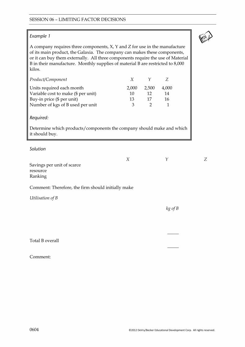
SESSION 06 – LIMITING FACTOR DECISIONS
0604 ©2012 DeVry/Becker Educational Development Corp. All rights reserved.
Example 1
A company requires three components, X, Y and Z for use in the manufacture of its main product, the Galaxia. The company can makes these components, or it can buy them externally. All three components require the use of Material B in their manufacture. Monthly supplies of material B are restricted to 8,000 kilos.
Product/Component X Y Z
Units required each month 2,000 2,500 4,000 Variable cost to make ($ per unit) 10 12 14 Buy-in price ($ per unit) 13 17 16 Number of kgs of B used per unit 3 2 1
Required:
Determine which products/components the company should make and which it should buy.
Solution
X Y Z Savings per unit of scarce resource
Ranking Comment: Therefore, the firm should initially make
Utilisation of B
kg of B
Total B overall
_____
_____
Comment:
SESSION 06 – LIMITING FACTOR DECISIONS
©2012 DeVry/Becker Educational Development Corp. All rights reserved. 0605
3 MULTI-LIMITING FACTORS
3.1 Linear programming
In situations where more than one factor is limited, an alternative approach is used to determine the optimal production so as to maximise contribution (and therefore profit). This technique is linear programming:
A mathematical technique for problems of rationing scarce resources among “products” to achieve optimum benefit.
Objective function – quantifies the objective. For example:
profit maximisation (which is always by maximising contribution); cost minimisation.
Based on the assumption that the objective and the constraints may be expressed as linear equations.
The syllabus only includes situations involving two variables – this allows the equations to be plotted as straight lines on a graph.
The graph can be used to identify the optimal solution.
The optimal solution must be solved algebraically (e.g. using simultaneous equations).
Commentary Do not merely read from the graph – it is relatively crude and although it should be sufficiently reliable to identify the optimal solution it should not be relied on to specify the solution.
3.2 Step by step approach
Step 1 Define unknowns.
Step 2 Formulate the objective function (use contribution not profit).
Step 3 Express constraints in terms of inequalities (including non-negativity).
Step 4 Plot all constraints on a graph and identify the feasible region.
Step 5 Plot the objective function and identify the optimal point.
Step 6 Solve (algebraically if necessary) for the unknowns at the optimal point.
Step 7 Answer the question set.
SESSION 06 – LIMITING FACTOR DECISIONS
0606 ©2012 DeVry/Becker Educational Development Corp. All rights reserved.
3.3 Problem formulation
Illustration 1
A company makes two products, cabinets and chests. Each product passes through two departments, carpentry and polishing. The time spent in each department is as follows. Departmental time (hours) Carpentry Polishing
Cabinets 3 2 Chests 4 6
There are 4,800 hours available in each department.
Annual production of cabinets must not exceed 1,200 units. Apart from this, all items produced can be sold.
The contribution to profit and fixed overheads is $100 for a cabinet and $150 for a chest.
Required:
Calculate the optimal product mix which will maximise the total contribution to profit.
Solution
Step 1 — Define unknowns
Let: x = number of cabinets to be produced per annum y = number of chests to be produced per annum C = total contribution to profit Step 2 — Formulate the objective function
The function to be maximised is the total contribution to profit (i.e. C). Since cabinets and chests contribute $100 and $150 respectively, for each item produced
C = 100x + 150y Step 3 — Formulate constraints
4,800 carpentry hours are available to provide 3 hours per cabinet and 4 hours per chest:
3 4x y+ ≤ 4,800
4,800 polishing hours are available to provide 2 hours per cabinet and 6 hours per chest:
2 6x y+ ≤ 4,800
Production of cabinets must not exceed 1,200 units: x ≤ 1,200
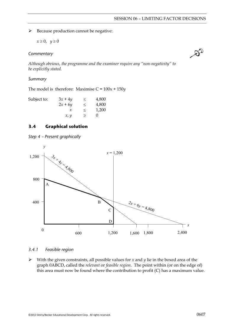
SESSION 06 – LIMITING FACTOR DECISIONS
©2012 DeVry/Becker Educational Development Corp. All rights reserved. 0607
Because production cannot be negative:
x ≥ 0, y ≥ 0
Commentary Although obvious, the programme and the examiner require any “non-negativity” to be explicitly stated.
Summary
The model is therefore: Maximise C = 100x + 150y
Subject to: 3x + 4y ≤ 4,800 2x + 6y ≤ 4,800 x ≤ 1,200 x, y ≥ 0 3.4 Graphical solution
Step 4 — Present graphically
600 1,200 1,600 1,800 2,400
1,200
800
400
0x
yx = 1,200
A
B
C
D
3x + 4y = 4,800
2x + 6y = 4,800
3.4.1 Feasible region
With the given constraints, all possible values for x and y lie in the boxed area of the graph 0ABCD, called the relevant or feasible region. The point within (or on the edge of) this area must now be found where the contribution to profit (C) has a maximum value.
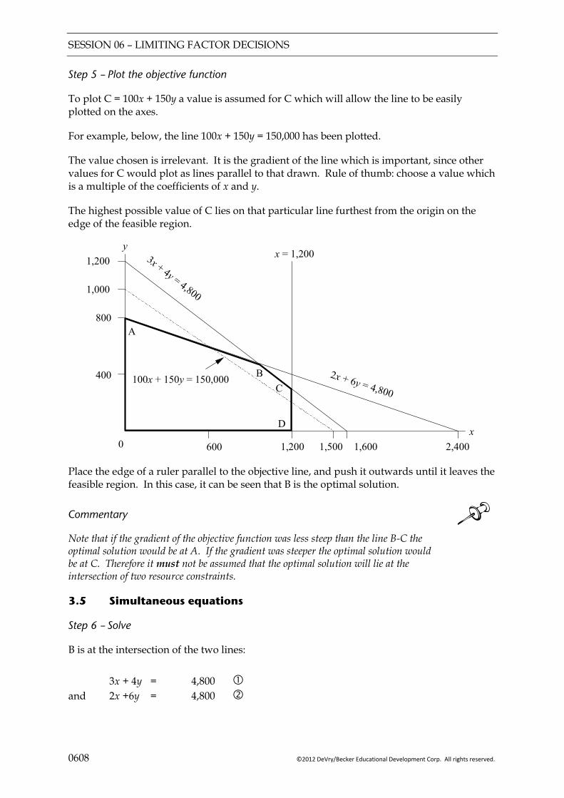
SESSION 06 – LIMITING FACTOR DECISIONS
0608 ©2012 DeVry/Becker Educational Development Corp. All rights reserved.
Step 5 — Plot the objective function
To plot C = 100x + 150y a value is assumed for C which will allow the line to be easily plotted on the axes.
For example, below, the line 100x + 150y = 150,000 has been plotted.
The value chosen is irrelevant. It is the gradient of the line which is important, since other values for C would plot as lines parallel to that drawn. Rule of thumb: choose a value which is a multiple of the coefficients of x and y.
The highest possible value of C lies on that particular line furthest from the origin on the edge of the feasible region.
600 1,200 1,600 2,400
1,200
800
400
0x
yx = 1,200
A
BC
D
3x + 4y = 4,800
2x + 6y = 4,800
1,000
100x + 150y = 150,000
1,500
Place the edge of a ruler parallel to the objective line, and push it outwards until it leaves the feasible region. In this case, it can be seen that B is the optimal solution.
Commentary Note that if the gradient of the objective function was less steep than the line B-C the optimal solution would be at A. If the gradient was steeper the optimal solution would be at C. Therefore it must not be assumed that the optimal solution will lie at the intersection of two resource constraints.
3.5 Simultaneous equations
Step 6 — Solve
B is at the intersection of the two lines:
3x + 4y = 4,800 and 2x +6y = 4,800
SESSION 06 – LIMITING FACTOR DECISIONS
©2012 DeVry/Becker Educational Development Corp. All rights reserved. 0609
Solving simultaneously:
1½ × 3x + 9y = 7,200 (new equation ) 3x + 4y = 4,800 (original equation )
– 5y = 2,400
Therefore y = 480
Substitute for y in (1):
3x + 1,920 = 4,800 3x = 2,880
Therefore x = 960
3.6 Optimal solution
The optimal solution is to produce 960 cabinets and 480 chests.
This will give a contribution of C = 100x + 150y = ($100 × 960) + ($150 × 480) = $168,000
Example 2
A manufacturer produces two types of garden furniture – tables and benches. Both use the same material and are produced by the same workforce, which consists of skilled and unskilled workers. The managing director is trying to decide on the optimal production plan to maximise contribution each week.
The following standard cost cards apply:
Table Bench $ $
Material ($5/kg) 15 10 Skilled labour ($10/hour) 50 20 Unskilled labour ($4/hour) 16 4 Variable overhead ($2/hour) 18 6 ___ ___
Total variable cost 99 40 Selling price 134 50 ___ ___
Contribution per unit 35 10 ___ ___ There is a shortage of the required material and only 120 kilos are available each week. There are four skilled workmen, each working a 35-hour week. Unskilled labour is employed on a part-time basis and there are 100 hours available per week.
Required:
Determine graphically how many units of each type of furniture should be produced each week to maximise contribution. Calculate the maximum weekly contribution.

SESSION 06 – LIMITING FACTOR DECISIONS
0610 ©2012 DeVry/Becker Educational Development Corp. All rights reserved.
Solution
Let x be
Let y be
Objective function to maximise contribution ©, given by
Subject to constraints:
Materials
Skilled labour
Unskilled labour
Non negative
From the graph
SESSION 06 – LIMITING FACTOR DECISIONS
©2012 DeVry/Becker Educational Development Corp. All rights reserved. 0611
SESSION 06 – LIMITING FACTOR DECISIONS
0612 ©2012 DeVry/Becker Educational Development Corp. All rights reserved.
Feasible region is
A sample contribution line, C = 700
The optimum point is at
Solving simultaneously:
So to maximise contribution, the company should
The contribution will be
3.7 Assumptions
The following assumptions give rise to limitations using the graphical method:
Linearity – contribution per unit and resource utilisation per unit are same for any quantity produced and sold in the range under consideration.
Infinite divisibility – of products and resources. Solution may not have integer values (e.g. 121/4 units of x and 93/4 units of y) and should not be rounded. For example, for an optimisation problem:
rounding up will be to a point outside the feasible region; if rounding down, it will depend on the gradient of the objective function which
integer value lies furthest from the origin.
Solution is dependent on the quality of input data:
Complete; Accurate; Valid.
Only one quantifiable objective can be satisfied. Non-quantifiable objectives are not considered at all.
Single value estimates (e.g. expected values) can be used for uncertain variables.
Only two “products” for graphical solution (but see below).

SESSION 06 – LIMITING FACTOR DECISIONS
©2012 DeVry/Becker Educational Development Corp. All rights reserved. 0613
4 FURTHER CONSIDERATIONS
4.1 Shadow price
The shadow price (or dual price) is a term that is applied to limited resources. It is the additional contribution that the company would generate if one more unit of the resource were made available.
The significance of the shadow price is that companies may be able to obtain additional quantities of a scarce resource if they are prepared to pay a higher price. The shadow price represents the maximum premium over the normal price that the company would be prepared to pay for each additional unit.
It is not worth paying more than the normal price plus the shadow price for additional units, as the additional contribution from producing extra units is more than offset by the extra price paid.
Illustration 2
In Example 4 there are only 100 hours of unskilled labour available. Solving Example 4 using linear programming demonstrated that the maximum contribution that can be generated each week is $900, if 20 tables and 20 benches are made. Additional unskilled labour hours may be available at a premium rate.
Required:
Calculate the shadow price of unskilled labour
Solution
The constraint for unskilled labour now becomes: 4x + y ≤ 101.
The other constraints remain the same. In summary therefore it is necessary to solve the linear program:
Objective function to maximise contribution (C) given by: C =35 x + 10 y
Subject to constraints:
Materials: 3x + 2y ≤ 120
Skilled labour: 5x + 2y ≤ 140
Unskilled labour: 4 x + y ≤ 101
Non negativity: x≥ 0, y ≥ 0.
Plotting the equations graphically:

SESSION 06 – LIMITING FACTOR DECISIONS
0614 ©2012 DeVry/Becker Educational Development Corp. All rights reserved.
101
0
10
20
30
40
50
60
70
80
90
5 10 15 20 25 30 35 40
Unskilled labour
Skilled labour
Materials
A
C
D
Tables
B
Benches
The feasible region is OABCD.
A sample contribution line, C= 700 is represented by the broken line.
Since the unskilled labour equation has changed, the line showing the skilled labour constraint becomes very slightly steeper. The optimal point C is the intersection of the skilled and unskilled constraints:
Solving simultaneously
5x + 2y = 140 (1) 4x + y = 101 (2)
2 × (2) 8x + 2y = 202 (3) (3) – (1) 3x = 62 x = 20.67
By substitution in (2)
82.68 + y = 101 y = 18.32
Contribution becomes (20.67 x $35) + (18.32 x $10) = $906.65.
This compares to contribution of $900 when only 100 hours of unskilled labour were available (see Example 4 solution).
This means that the availability of 1 additional hour of unskilled labour increases contribution by $6.65. This is the shadow price of unskilled labour.
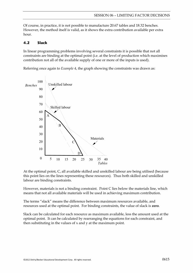
SESSION 06 – LIMITING FACTOR DECISIONS
©2012 DeVry/Becker Educational Development Corp. All rights reserved. 0615
Of course, in practice, it is not possible to manufacture 20.67 tables and 18.32 benches. However, the method itself is valid, as it shows the extra contribution available per extra hour.
4.2 Slack
In linear programming problems involving several constraints it is possible that not all constraints are binding at the optimal point (i.e. at the level of production which maximises contribution not all of the available supply of one or more of the inputs is used).
Referring once again to Example 4, the graph showing the constraints was drawn as:
100
0
10
20
30
40
50
60
70
80
90
5 10 15 20 25 30 35 40
Unskilled labour
Skilled labour
Materials
A
C
D
Tables
B
Benches
At the optimal point, C, all available skilled and unskilled labour are being utilised (because this point lies on the lines representing these resources). Thus both skilled and unskilled labour are binding constraints.
However, materials is not a binding constraint. Point C lies below the materials line, which means that not all available materials will be used in achieving maximum contribution.
The terms “slack” means the difference between maximum resources available, and resources used at the optimal point. For binding constraints, the value of slack is zero.
Slack can be calculated for each resource as maximum available, less the amount used at the optimal point. It can be calculated by rearranging the equations for each constraint, and then substituting in the values of x and y at the maximum point.
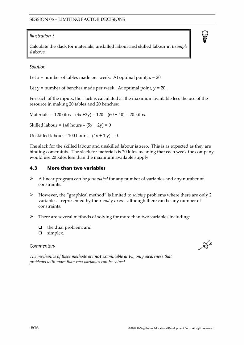
SESSION 06 – LIMITING FACTOR DECISIONS
0616 ©2012 DeVry/Becker Educational Development Corp. All rights reserved.
Illustration 3
Calculate the slack for materials, unskilled labour and skilled labour in Example 4 above
Solution
Let x = number of tables made per week. At optimal point, x = 20
Let y = number of benches made per week. At optimal point, y = 20.
For each of the inputs, the slack is calculated as the maximum available less the use of the resource in making 20 tables and 20 benches:
Materials: = 120kilos – (3x +2y) = 120 – (60 + 40) = 20 kilos.
Skilled labour = 140 hours – (5x + 2y) = 0
Unskilled labour = 100 hours – (4x + 1 y) = 0.
The slack for the skilled labour and unskilled labour is zero. This is as expected as they are binding constraints. The slack for materials is 20 kilos meaning that each week the company would use 20 kilos less than the maximum available supply.
4.3 More than two variables
A linear program can be formulated for any number of variables and any number of constraints.
However, the “graphical method” is limited to solving problems where there are only 2 variables – represented by the x and y axes – although there can be any number of constraints.
There are several methods of solving for more than two variables including:
the dual problem; and simplex.
Commentary The mechanics of these methods are not examinable at F5, only awareness that problems with more than two variables can be solved.

SESSION 06 – LIMITING FACTOR DECISIONS
©2012 DeVry/Becker Educational Development Corp. All rights reserved. 0617
Key points
Where factors of production are scarce, production decisions have to be made to maximise contribution (and hence profit) given limited resources.
Where one resource is scarce, the approach is to rank products by contribution generated per unit of scarce resource.
For make or buy decisions the method is to rank products by saving per unit of scarce resource.
Where there is more than one constraint, use linear programming:
(1) Define variables;
(2) Define the objective function (usually to maximise contribution);
(3) Formulate constraints;
(4) Plot constraints on a graph and determine the feasible area;
(5) Draw a sample contribution line and use this to find the point on the feasible region which generates the highest contribution.
(6) Solve the equation(s) for the optimal point in (5) to specify the corresponding values of the variables.
(7) Answer the question. Maximum profit MUST be calculated as maximum contribution less total fixed overheads never using unit profit!
The shadow price of a resource is the amount by which contribution would be increased if one more unit of the scarce resource was available.
Slack arises where the company does not use all of the resource available. Slack can be calculated as resource available less resource used.

SESSION 06 – LIMITING FACTOR DECISIONS
0618 ©2012 DeVry/Becker Educational Development Corp. All rights reserved.
FOCUS
You should now be able to:
identify limiting factors in a scarce resource situation and select an appropriate
technique;
determine the optimal production plan where an organisation is restricted by a simple limiting factor, including within the context of “make” or “buy” decisions;
formulate and solve a multiple scarce resource program both graphically and using simultaneous equations as appropriate;
explain and calculate shadow prices (dual prices) and discuss their implications on decision-making and performance management;
calculate slack and explain the implications of the existence of slack for decision making and performance management;
explain the issues surrounding make vs buy and outsourcing decisions;
calculate and compare make costs with buy in costs;
compare in -house costs and outsource costs of completing tasks and consider other issues surrounding this decision;
apply relevant costing principles in situations involving shut down, one off contracts and the further processing of joint costs.

SESSION 06 – LIMITING FACTOR DECISIONS
©2012 DeVry/Becker Educational Development Corp. All rights reserved. 0619
EXAMPLE SOLUTIONS
Solution 1 — Make or buy
X Y Z Savings per unit of scarce resource 3
10 13 − = 1 2
12 17 − = 2.5
114 16 − = 2
Ranking Comment: Therefore, the firm should initially make Ys and then make as many Zs as possible.
Utilisation of B
kg of B 2,500 Ys × 2 kg each uses 3,000 Zs × 1 kg each uses
5,000 3,000
Total B overall
_____ 8,000 _____
Comment: The additional 1,000 Zs and 2,000 Xs required should be bought in.
Solution 2 — Linear program
Let x be the number of tables made per week Let y be the number of benches made per week
Objective function to maximise contribution (C), given by 35x + 10y
Subject to constraints
Materials 3x + 2y ≤ 120 Skilled labour 5x + 2y ≤ 140 Unskilled labour 4x + y ≤ 100 Non negative x, y ≥ 0
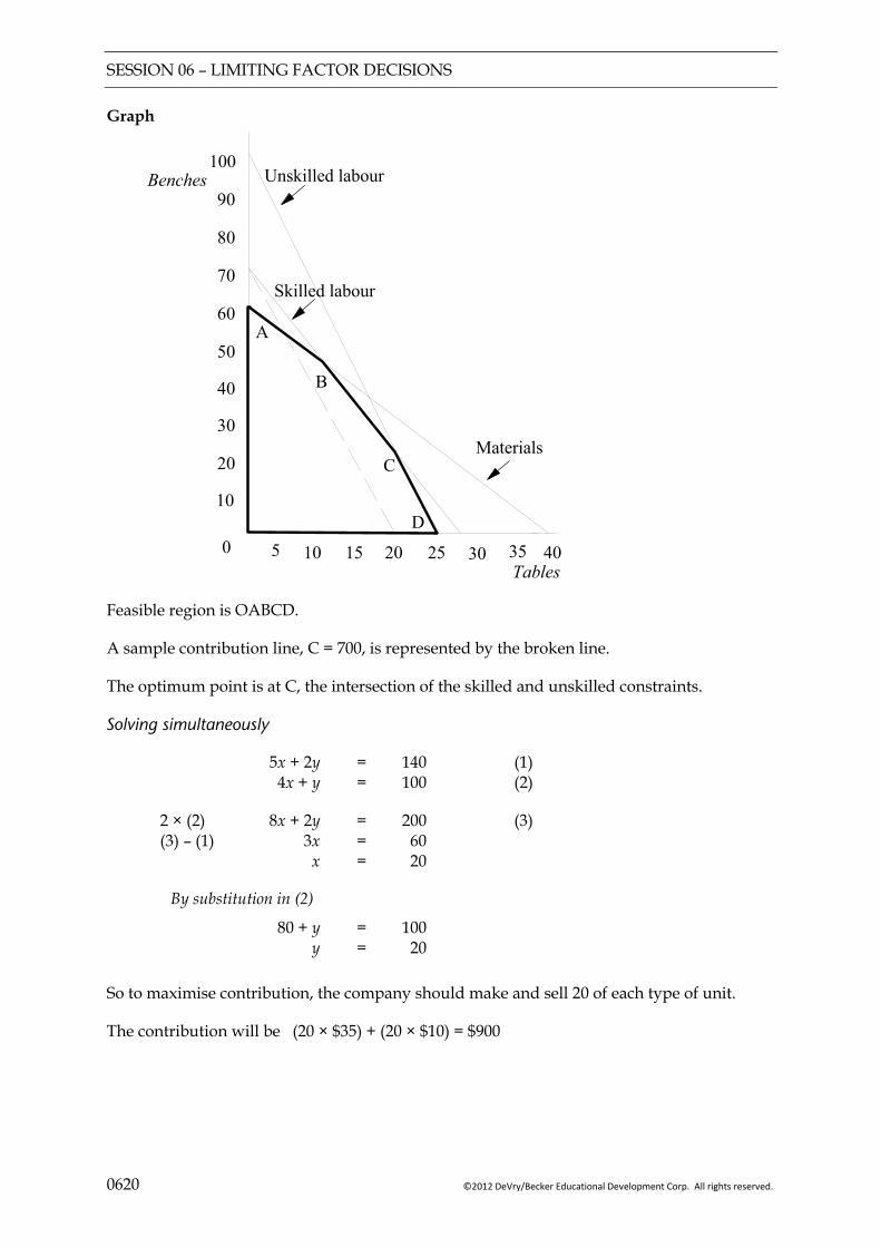
SESSION 06 – LIMITING FACTOR DECISIONS
0620 ©2012 DeVry/Becker Educational Development Corp. All rights reserved.
Graph
100
0
10
20
30
40
50
60
70
80
90
5 10 15 20 25 30 35 40
Unskilled labour
Skilled labour
Materials
A
C
D
Tables
B
Benches
Feasible region is OABCD.
A sample contribution line, C = 700, is represented by the broken line.
The optimum point is at C, the intersection of the skilled and unskilled constraints.
Solving simultaneously
5x + 2y = 140 (1) 4x + y = 100 (2)
2 × (2) 8x + 2y = 200 (3) (3) – (1) 3x = 60 x = 20
By substitution in (2)
80 + y = 100 y = 20
So to maximise contribution, the company should make and sell 20 of each type of unit.
The contribution will be (20 × $35) + (20 × $10) = $900
SESSION 07 – PRICING
©2012 DeVry/Becker Educational Development Corp. All rights reserved. 0701
OVERVIEW
Objective
To identify, discuss and implement a range of product-pricing methods applicable in particular market situations.
FACTORS INFLUENCING PRICE
THE ECONOMIST’S
MODEL
PRICING
OTHER PRICING POLICIES
Demand curve Elasticity of demand Marginal revenue Marginal cost Profit maximising output
ACCOUNTANT’SMETHOD
COST PLUS OPPORTUNITY COST PRICING
Full cost Marginal cost
When used Limitations
RETURN ON INVESTMENT
PRICING
Target return Advantages Disadvantages
Market skimming Market penetration Complementary product Price discrimination Loss leaders Going-rate pricing Product-line pricing
Level of demand Elasticity of demand The product life cycle Competitors Customers

SESSION 07 – PRICING
0702 ©2012 DeVry/Becker Educational Development Corp. All rights reserved.
1 COST PLUS
1.1 Full cost plus pricing
$/unit Direct production costs X
Absorption of overheads Variable production overhead Fixed production overhead Variable non-production overhead Fixed non-production overhead
X X X X
Full cost Mark-up %
___ X X
Selling price
___ X ___
Selling price per unit =
units sales BudgetedupMark cost production-non budgeted total cost production budgeted Total ++
1.1.1 Advantages
If the budget sales level is achieved, profit will be made.
The full cost should be readily available if a system of standard costing is in operation.
Appropriate where fixed costs are significant.
Useful for justifying prices (and price rises).
Simple and cheap to operate.
1.1.2 Disadvantages
The method of accounting for overheads will have a large impact on the costs calculated for different products.
If actual sales are below budget, losses may occur.
Ignores external factors (e.g. demand/price relationship, competitors’ prices).
Size of mark-up is arbitrary.
May not maximise profits.
Full cost plus pricing is a long-term pricing method. It ensures prices cover all variable and fixed costs.
SESSION 07 – PRICING
©2012 DeVry/Becker Educational Development Corp. All rights reserved. 0703
The problems regarding overheads can be reduced by using activity based costing. This simply means that the cost per unit of the product is calculated using activity based costing (see Session 2). A margin is added to this cost.
1.2 Marginal cost plus pricing
Selling price per unit =
units sales Budgetedupmark cost production-non variablebudgeted cost production variableBudgeted ++
1.2.1 Advantages
Mark-up represents contribution – useful in short-run pricing decisions (e.g. market penetration policy).
Appropriate where fixed costs are relatively small.
1.2.2 Disadvantages
May lead to failure to recover fixed costs.
Not appropriate for long-term pricing, particularly where fixed costs are significant.
2 RETURN ON INVESTMENT PRICING
2.1 Target return
Prices are set to achieve a target percentage return on the capital invested in production.
Unit selling price = units sales Budgeted
employed) capital % (target cost full Budgeted ×+
2.2 Advantages
Links price to both short-term costs and long-term capital employed Consistent with ROI as a performance measure. Target ROI can be set to take account of risk.
2.3 Disadvantages
Ignores external factors. Problems in calculating capital employed (e.g. whether to use book values or
replacement cost). Subjective split of shared investment between products.
ROI pricing is a long-term pricing method.
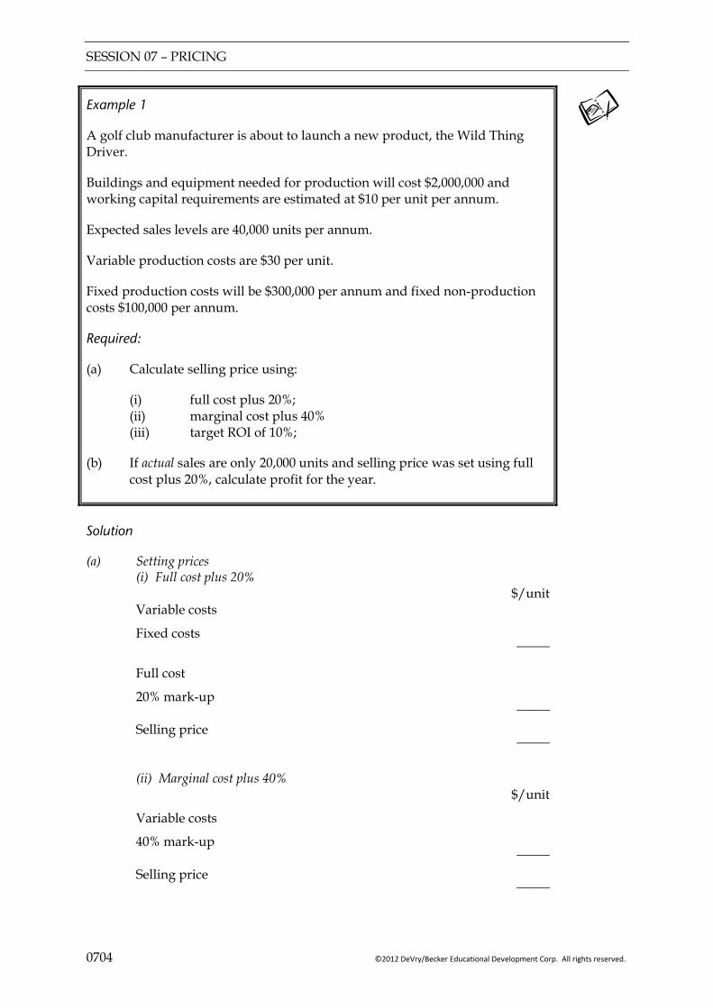
SESSION 07 – PRICING
0704 ©2012 DeVry/Becker Educational Development Corp. All rights reserved.
Example 1
A golf club manufacturer is about to launch a new product, the Wild Thing Driver.
Buildings and equipment needed for production will cost $2,000,000 and working capital requirements are estimated at $10 per unit per annum.
Expected sales levels are 40,000 units per annum.
Variable production costs are $30 per unit.
Fixed production costs will be $300,000 per annum and fixed non-production costs $100,000 per annum.
Required:
(a) Calculate selling price using:
(i) full cost plus 20%; (ii) marginal cost plus 40% (iii) target ROI of 10%;
(b) If actual sales are only 20,000 units and selling price was set using full cost plus 20%, calculate profit for the year.
Solution
(a) Setting prices (i) Full cost plus 20% $/unit Variable costs
Fixed costs
Full cost
20% mark-up
_____
Selling price
_____ _____
(ii) Marginal cost plus 40% $/unit Variable costs
40% mark-up
Selling price
_____ _____
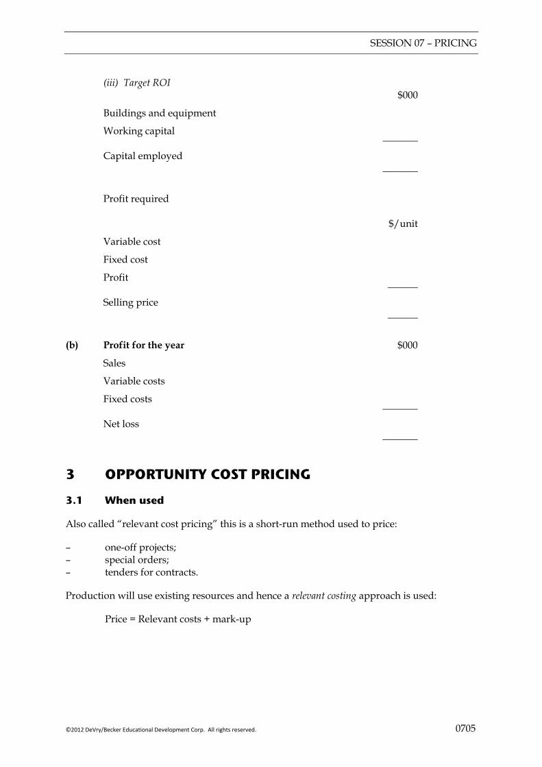
SESSION 07 – PRICING
©2012 DeVry/Becker Educational Development Corp. All rights reserved. 0705
(iii) Target ROI $000 Buildings and equipment
Working capital
Capital employed
_______
_______ Profit required $/unit Variable cost
Fixed cost
Profit
Selling price
______
______ (b) Profit for the year $000 Sales
Variable costs
Fixed costs
Net loss
_______
_______ 3 OPPORTUNITY COST PRICING
3.1 When used
Also called “relevant cost pricing” this is a short-run method used to price:
– one-off projects; – special orders; – tenders for contracts.
Production will use existing resources and hence a relevant costing approach is used:
Price = Relevant costs + mark-up

SESSION 07 – PRICING
0706 ©2012 DeVry/Becker Educational Development Corp. All rights reserved.
Example 2
After spending $500 on market research, Bobco Engineering wants to bid on an important one-off contract and needs to ensure its costing is both competitive and commercially rational. To complete the project, it will need to devote the following resources to its construction:
1,500 kg of standard steel regularly used in its production process. Its currently has inventory of 6,000 kg purchased at an average price of $8/kg. With recent market conditions, purchase cost is now $9.35/kg.
500 kg of specialty steel. It has 500 kg of such steel in inventory. This was purchased 16 months ago at $12/kg. As it has not been used since purchasing, the auditors insisted on a write-down to estimated net realizable value of $4/kg. The purchasing manager figures he can sell it for scrap at $2/kg. Costs to remove it from the warehouse and deliver it would be $1,000.
380 hours of unskilled labour. While the existing union contract pays $6/hour for such labour, extra workers would have to be hired in the “temporary” labour market at $7/hour.
196 hours of semi-skilled being paid $9/hour under the existing union contract. Currently there is a surplus of such labour in the plant.
51 hours of skilled labour being paid $18/hour under the current union contract. The workers are currently busy in another department where they are producing output that is sold for $96 and that uses $15 of direct material, $9 of skilled labour, $27 of semi-skilled labour, $15 of variable overheads and $8 fixed cost overheads allocated. It takes ½ hour of skilled labour to work on this product. The department head has agreed to release “his” skilled workers but must be compensated so he is no worse off.
Use of equipment which was scheduled to be disposed of this period for $12,000. If used in the project, it will have to be disposed of later at an estimated selling price of $4,000.
Exclusive use of a piece of manufacturing equipment (a fribulator) that will not survive its use in the project. The machine originally cost $51,000 and currently has a carrying (i.e. “book”) value of $6,000. It could be currently sold in the used fribulator market for $8,000 (since new ones now cost $45,000). If it was left in its existing use, it could generate cash flows with an estimated present value of $5,000.
38 kg of Ecotox which was originally purchased for $600/kg. Under current government environmental rules, Bobco will have to pay $3,000 for the recycling company to take it away if it is not used in the contract.
Required:
Calculate the price that Bobco should bid for the contract on the assumption that it wishes to charge a price equal to relevant cost plus 25%.
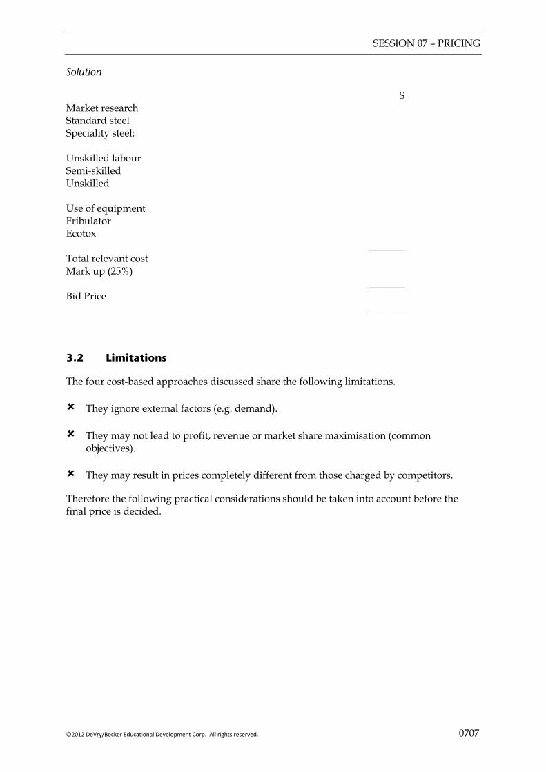
SESSION 07 – PRICING
©2012 DeVry/Becker Educational Development Corp. All rights reserved. 0707
Solution
$ Market research Standard steel Speciality steel: Unskilled labour Semi-skilled Unskilled Use of equipment Fribulator Ecotox _______ Total relevant cost Mark up (25%) _______ Bid Price _______
3.2 Limitations
The four cost-based approaches discussed share the following limitations.
They ignore external factors (e.g. demand).
They may not lead to profit, revenue or market share maximisation (common objectives).
They may result in prices completely different from those charged by competitors.
Therefore the following practical considerations should be taken into account before the final price is decided.

SESSION 07 – PRICING
0708 ©2012 DeVry/Becker Educational Development Corp. All rights reserved.
4 ECONOMIST’S MODEL
4.1 Demand curve
4.1.1 The concept
Demand means the total quantity of a product or service that the buyers in a market would wish to buy in a given period.
It depends on the price charged by suppliers. For most goods, as the price falls, demand for the goods rises.
This can be shown graphically as follows:
4.1.1 Equation
The demand curve can be expressed as an equation of the form:
P = a + bQ
Where:
P is the price that would achieve a given demand, Q;
a is the price at which demand would be zero;
b is the slope of the line – it shows by how much the price must change to achieve a given increase in demand:
b = quantityin change
pricein change
b is normally negative (i.e. as the price falls, demand rises).
Price $
Demand (Units)
a
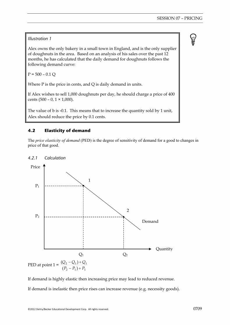
SESSION 07 – PRICING
©2012 DeVry/Becker Educational Development Corp. All rights reserved. 0709
Illustration 1
Alex owns the only bakery in a small town in England, and is the only supplier of doughnuts in the area. Based on an analysis of his sales over the past 12 months, he has calculated that the daily demand for doughnuts follows the following demand curve:
P = 500 – 0.1 Q
Where P is the price in cents, and Q is daily demand in units.
If Alex wishes to sell 1,000 doughnuts per day, he should charge a price of 400 cents (500 – 0, 1 × 1,000).
The value of b is -0.1. This means that to increase the quantity sold by 1 unit, Alex should reduce the price by 0.1 cents.
4.2 Elasticity of demand
The price elasticity of demand (PED) is the degree of sensitivity of demand for a good to changes in price of that good.
4.2.1 Calculation
Price
Quantity
Demand
Q1 Q2
P1
P2
•
•
1
2
PED at point 1 =
112
112
)()(
PPPQQQ
÷−÷−
If demand is highly elastic then increasing price may lead to reduced revenue.
If demand is inelastic then price rises can increase revenue (e.g. necessity goods).
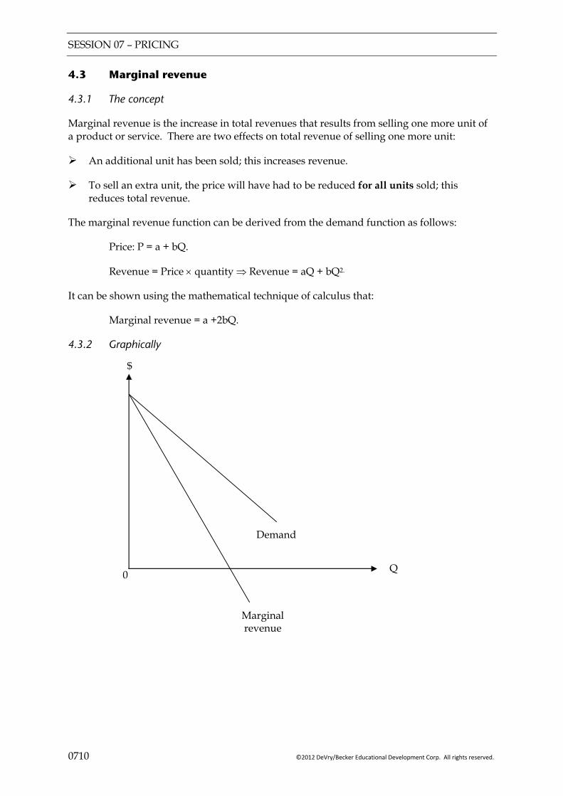
SESSION 07 – PRICING
0710 ©2012 DeVry/Becker Educational Development Corp. All rights reserved.
4.3 Marginal revenue
4.3.1 The concept
Marginal revenue is the increase in total revenues that results from selling one more unit of a product or service. There are two effects on total revenue of selling one more unit:
An additional unit has been sold; this increases revenue.
To sell an extra unit, the price will have had to be reduced for all units sold; this reduces total revenue.
The marginal revenue function can be derived from the demand function as follows:
Price: P = a + bQ.
Revenue = Price × quantity ⇒ Revenue = aQ + bQ2.
It can be shown using the mathematical technique of calculus that:
Marginal revenue = a +2bQ.
4.3.2 Graphically
$
Q 0
Marginal revenue
Demand
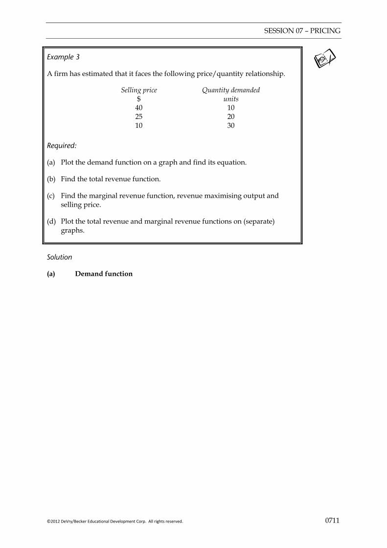
SESSION 07 – PRICING
©2012 DeVry/Becker Educational Development Corp. All rights reserved. 0711
Example 3
A firm has estimated that it faces the following price/quantity relationship.
Selling price Quantity demanded $ units 40 10 25 20 10 30
Required:
(a) Plot the demand function on a graph and find its equation.
(b) Find the total revenue function.
(c) Find the marginal revenue function, revenue maximising output and selling price.
(d) Plot the total revenue and marginal revenue functions on (separate) graphs.
Solution
(a) Demand function
SESSION 07 – PRICING
0712 ©2012 DeVry/Becker Educational Development Corp. All rights reserved.
(b) Total revenue, TR =
(c) Marginal revenue, MR =
Revenue maximisation is where MR = 0
q =
Substitute into demand function to find revenue maximising selling price:
p =
Maximum revenue =
(d) Graphs
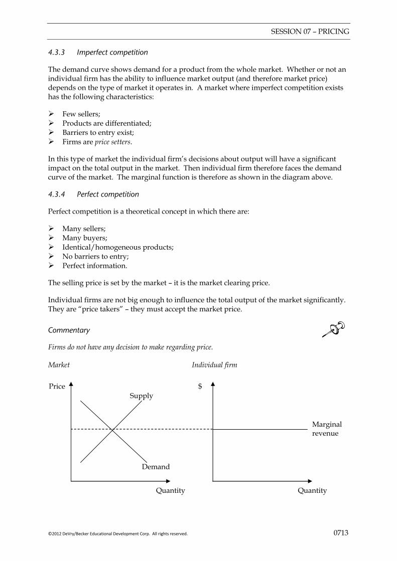
SESSION 07 – PRICING
©2012 DeVry/Becker Educational Development Corp. All rights reserved. 0713
4.3.3 Imperfect competition
The demand curve shows demand for a product from the whole market. Whether or not an individual firm has the ability to influence market output (and therefore market price) depends on the type of market it operates in. A market where imperfect competition exists has the following characteristics:
Few sellers; Products are differentiated; Barriers to entry exist; Firms are price setters.
In this type of market the individual firm’s decisions about output will have a significant impact on the total output in the market. Then individual firm therefore faces the demand curve of the market. The marginal function is therefore as shown in the diagram above.
4.3.4 Perfect competition
Perfect competition is a theoretical concept in which there are:
Many sellers; Many buyers; Identical/homogeneous products; No barriers to entry; Perfect information.
The selling price is set by the market – it is the market clearing price.
Individual firms are not big enough to influence the total output of the market significantly. They are “price takers” – they must accept the market price.
Commentary Firms do not have any decision to make regarding price. Market Individual firm
Price $ Supply
Demand
Quantity Quantity
Marginalrevenue

SESSION 07 – PRICING
0714 ©2012 DeVry/Becker Educational Development Corp. All rights reserved.
If an individual firm charges a price higher than the market price, that firm will not make any sales, since buyers have perfect information, and will know that they can buy at a lower price from the other suppliers in the market.
There is no incentive for firms to sell for a price below the market price since the firm could sell all of its output for the market price.
In a competitive market therefore, firms will charge the market price.
4.4 Marginal cost
This is the increase in total cost from producing and selling an additional unit of a product or service.
Economists assume that marginal cost changes as output increases. Initially marginal cost falls, as output rises, due to economies of scale. Once the firm reaches its lowest marginal cost, however, marginal cost begins to rise as output increases further.
Accountants (and examiners) take a simpler approach and assume that marginal cost is equal to variable cost per unit (at least until full capacity is reached).
4.5 Maximising profits
In the economist’s model, firms do not make a decision about price but about the quantity of output. Price is then determined by the demand curve.
To maximise profits, firms should produce the quantity where:
Marginal cost = Marginal revenue
Diagrammatically
$
Profit maximising
output
Q
Marginal cost
0
Marginal revenue
Demand
Profit maximising
price
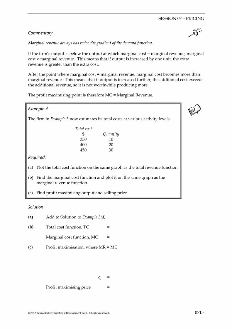
SESSION 07 – PRICING
©2012 DeVry/Becker Educational Development Corp. All rights reserved. 0715
Commentary Marginal revenue always has twice the gradient of the demand function. If the firm’s output is below the output at which marginal cost = marginal revenue, marginal cost > marginal revenue. This means that if output is increased by one unit, the extra revenue is greater than the extra cost.
After the point where marginal cost = marginal revenue, marginal cost becomes more than marginal revenue. This means that if output is increased further, the additional cost exceeds the additional revenue, so it is not worthwhile producing more.
The profit maximising point is therefore MC = Marginal Revenue.
Example 4
The firm in Example 3 now estimates its total costs at various activity levels:
Total cost $ Quantity 350 10 400 20 450 30
Required:
(a) Plot the total cost function on the same graph as the total revenue function.
(b) Find the marginal cost function and plot it on the same graph as the marginal revenue function.
(c) Find profit maximising output and selling price.
Solution
(a) Add to Solution to Example 3(d)
(b) Total cost function, TC =
Marginal cost function, MC =
(c) Profit maximisation, where MR = MC
q =
Profit maximising price =
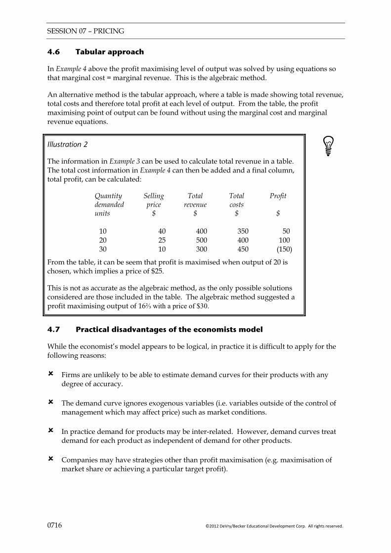
SESSION 07 – PRICING
0716 ©2012 DeVry/Becker Educational Development Corp. All rights reserved.
4.6 Tabular approach
In Example 4 above the profit maximising level of output was solved by using equations so that marginal cost = marginal revenue. This is the algebraic method.
An alternative method is the tabular approach, where a table is made showing total revenue, total costs and therefore total profit at each level of output. From the table, the profit maximising point of output can be found without using the marginal cost and marginal revenue equations.
Illustration 2
The information in Example 3 can be used to calculate total revenue in a table. The total cost information in Example 4 can then be added and a final column, total profit, can be calculated:
Quantity Selling Total Total Profit demanded price revenue costs units $ $ $ $ 10 40 400 350 50 20 25 500 400 100 30 10 300 450 (150)
From the table, it can be seem that profit is maximised when output of 20 is chosen, which implies a price of $25.
This is not as accurate as the algebraic method, as the only possible solutions considered are those included in the table. The algebraic method suggested a profit maximising output of 16⅔ with a price of $30.
4.7 Practical disadvantages of the economists model
While the economist’s model appears to be logical, in practice it is difficult to apply for the following reasons:
Firms are unlikely to be able to estimate demand curves for their products with any degree of accuracy.
The demand curve ignores exogenous variables (i.e. variables outside of the control of management which may affect price) such as market conditions.
In practice demand for products may be inter-related. However, demand curves treat demand for each product as independent of demand for other products.
Companies may have strategies other than profit maximisation (e.g. maximisation of market share or achieving a particular target profit).

SESSION 07 – PRICING
©2012 DeVry/Becker Educational Development Corp. All rights reserved. 0717
5 OTHER PRICING STRATEGIES
5.1 Market skimming
Set very high launch price for new product ( where customers are expected to pay more to be the first owners of a new product).
Must be “breakthrough” product (e.g. new technology).
May need to reduce prices later as competitors enter market.
Common in consumer electronics (e.g. wide-screen televisions).
5.2 Market penetration
Set low launch price when entering an already competitive market.
Gain market share.
Gain reputation.
Later increase price towards competitors’ prices.
Requires a price sensitive market.
5.3 Complementary product pricing
Where companies sell complementary products (e.g. computer hardware and software) the pricing strategy used for one of the products will affect demand for both products.
Therefore one product may be sold at a lower price to attract demand for the other.
5.4 Price discrimination
Sell a single product in different markets.
Set different price in each market.
Must be barriers between markets (e.g. geographical).
Increasingly difficult within EU due to legislation.
5.5 Loss leaders
Short run promotional offer on one product.
Sell very cheaply.
Attract customers to other products at normal price.
Often used in retailing (e.g. supermarkets).
5.6 Going-rate pricing
Set price at industry average.
Appropriate in competitive markets.

SESSION 07 – PRICING
0718 ©2012 DeVry/Becker Educational Development Corp. All rights reserved.
5.7 Product-line pricing
A product-line is a group of products that are closely related. This may be because they are sold to the same customer groups, or sold through the same outlets.
Product-line pricing involves setting the differentials between the prices of the various products in a product-line based on the difference costs of making the products, or the different features valued by the customers.
5.8 Volume discounting
Many organisations offer discounts for customers that buy a certain number of products. In retail stores for example, it is quite common to see “buy one, get one for 50%”.
The reason for using such a strategy is twofold:
To offer a more competitive price overall (as the average price paid for two items will obviously be lower than the price for one).
To acknowledge the law of “diminishing marginal utility” (i.e. the idea that the consumer gets most satisfaction from the first unit of a product or service). As subsequent units of a product or service are consumed, the satisfaction derived from them declines. Offering the second item for a lower price encourages consumers to buy it even though it offers less satisfaction.
5.9 Relevant cost pricing
Relevant cost pricing, also referred to as opportunity cost pricing, is often used for one-off contracts or orders. The relevant cost of the contract is calculated, and then a mark-up added to get the price. (See Example 2 earlier in this session.)
6 FACTORS INFLUENCING THE PRICE OF A PRODUCT
6.1 Level of demand
Demand is the quantity of a good which consumers want, and are willing and able to pay for. In practice, firms may not know what the demand curve for their product is. However, the level of demand will still influence pricing. If demand is high, firms would be able to charge a higher price for a product or service.
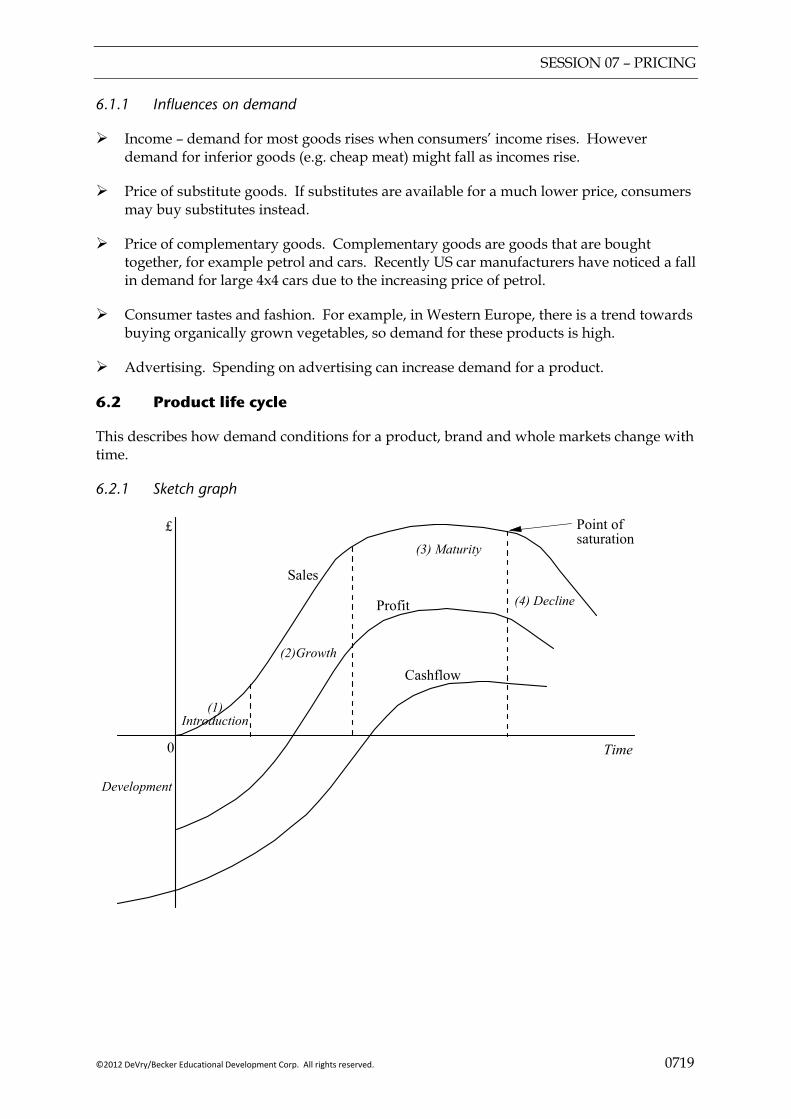
SESSION 07 – PRICING
©2012 DeVry/Becker Educational Development Corp. All rights reserved. 0719
6.1.1 Influences on demand
Income – demand for most goods rises when consumers’ income rises. However demand for inferior goods (e.g. cheap meat) might fall as incomes rise.
Price of substitute goods. If substitutes are available for a much lower price, consumers may buy substitutes instead.
Price of complementary goods. Complementary goods are goods that are bought together, for example petrol and cars. Recently US car manufacturers have noticed a fall in demand for large 4x4 cars due to the increasing price of petrol.
Consumer tastes and fashion. For example, in Western Europe, there is a trend towards buying organically grown vegetables, so demand for these products is high.
Advertising. Spending on advertising can increase demand for a product.
6.2 Product life cycle
This describes how demand conditions for a product, brand and whole markets change with time.
6.2.1 Sketch graph
Time
£
(2)Growth
(1) Introduction
(3) Maturity
(4) Decline
Cashflow
Profit
Sales
0
Development
Point ofsaturation
SESSION 07 – PRICING
0720 ©2012 DeVry/Becker Educational Development Corp. All rights reserved.
(1) Introduction phase/launch – special pricing strategies may be used during the launch of a new product such as market skimming, market penetration (see above). Companies also need to consider that the pricing strategy used at the introductory stage may affect demand in later years. For example, setting a low price initially may discourage competitors from entering the market, so allowing the company to enjoy higher demand later in the product life cycle.
(2) Growth – competition may rise due to new suppliers entering the market. This may force lower prices.
(3) Maturity – most profits are made during this phase. Prices may be stable. The company’s price strategy during this phase is more likely to focus on maximising short term profits, unlike in the introduction phase.
(4) Decline – prices may fall with demand unless a “niche” market can be found.
6.3 Competitors
If there are many competing suppliers in the market then an individual firm may have little power to influence prices.
On the other hand, a monopolist can dominate the market and set the price.
If a firm has competitors it must consider their possible reaction to its pricing policy. For example, cutting prices could lead to retaliation – a price war (this is common in supermarkets).
6.4 Customers
If the firm has one dominant customer it may find it difficult to increase prices and might be forced to offer bulk buying discounts.
Firms in the service sector sometimes try to attract “prestige” clients by offering low prices. The hope is the improve reputation and attract other clients (paying normal prices).
SESSION 07 – PRICING
©2012 DeVry/Becker Educational Development Corp. All rights reserved. 0721
Key points
Cost plus pricing methods involve adding a given margin to the cost of a product. The cost may be the marginal cost, the full cost, or even the relevant cost.
Cost plus methods of pricing do not consider external factors (e.g. what the market will pay for a product).
In the economist’s model, price is a function of the quantity supplied. As the quantity supplied rises, the price falls. The quantity provided is determined as the point where the marginal cost = marginal revenue.
Pricing is a strategic decision, and in practice there are several pricing strategies that may be adopted.
FOCUS
You should now be able to:
explain the factors that influence the pricing of a product or service;
explain the price elasticity of demand;
derive and manipulate a straight line demand equation. Derive an equation for the total cost function (including volume based discounts);
evaluate a decision to increase production and sales levels, considering incremental costs, incremental revenues and other factors;
explain different price strategies, including:
all forms of cost-plus; skimming; penetration; complementary product; product-line; volume discounting; discrimination; relevant cost;
calculate a price from a given strategy using cost-plus and relevant cost.

SESSION 07 – PRICING
0722 ©2012 DeVry/Becker Educational Development Corp. All rights reserved.
EXAMPLE SOLUTIONS
Solution 1 — Cost plus and target ROI
(a) Setting prices
(i) Full cost plus 20% $/unit Variable costs
Fixed costs 000,40
000,100000,300 +
30 10
Full cost 20% mark-up
__ 40
8
Selling price
__ 48 __
(ii) Marginal cost plus 40% $/unit Variable costs
40% mark-up 30 12
Selling price
__ 42 __
(iii) Target ROI $ Buildings and equipment
Working capital (10 × 40,000) 2,000,000
400,000
Capital employed
_________ 2,400,000 _________
Profit required = 2,400,000 × 10% = $240,000 $/unit Variable cost
Fixed cost
Profit 000,40000,240
30 10
6
Selling price
__ 46 __
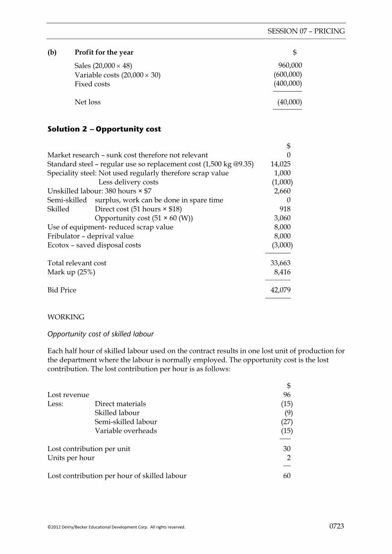
SESSION 07 – PRICING
©2012 DeVry/Becker Educational Development Corp. All rights reserved. 0723
(b) Profit for the year $
Sales (20,000 × 48) Variable costs (20,000 × 30) Fixed costs
960,000 (600,000) (400,000)
Net loss
________ (40,000) ________
Solution 2 — Opportunity cost
$ Market research – sunk cost therefore not relevant 0 Standard steel – regular use so replacement cost (1,500 kg @9.35) 14,025 Speciality steel: Not used regularly therefore scrap value 1,000 Less delivery costs (1,000) Unskilled labour: 380 hours × $7 2,660 Semi-skilled surplus, work can be done in spare time 0 Skilled Direct cost (51 hours × $18) 918 Opportunity cost (51 × 60 (W)) 3,060 Use of equipment- reduced scrap value 8,000 Fribulator – deprival value 8,000 Ecotox – saved disposal costs (3,000) _______
Total relevant cost 33,663 Mark up (25%) 8,416 _______
Bid Price 42,079 _______
WORKING
Opportunity cost of skilled labour
Each half hour of skilled labour used on the contract results in one lost unit of production for the department where the labour is normally employed. The opportunity cost is the lost contribution. The lost contribution per hour is as follows:
$ Lost revenue 96 Less: Direct materials (15) Skilled labour (9) Semi-skilled labour (27) Variable overheads (15) ___
Lost contribution per unit 30 Units per hour 2 __
Lost contribution per hour of skilled labour 60

SESSION 07 – PRICING
0724 ©2012 DeVry/Becker Educational Development Corp. All rights reserved.
Solution 3 — Revenue maximisation
(a) Demand function
Price
a 40 25 10
0 10 20 30 Quantity
x
x
x
b
demand
Equation of demand function, P
= a + bq
= 55 +
−−
10204025 q
= 55 – 1½q (b) Total revenue, TR = 55q – 1½q2
(c) Marginal revenue, MR = 55 – 3q
Revenue maximisation is where MR = 0 55 – 3q = 0 55 = 3q q = 18⅓ – revenue maximising output
Substitute into demand function to find revenue maximising selling price:
p = 55 – (1½ × 18⅓) $27½
Maximum revenue = 27.5 × 18⅓
$504.17

SESSION 07 – PRICING
©2012 DeVry/Becker Educational Development Corp. All rights reserved. 0725
(d) Graphs
$
500
400
300
200
100
x
x x
x
x
x
Total revenue
q
Total costs
10 18 31 20 30
10 16 32 20 30
$
25
5
0
–35
x
x
x
q
Marginal revenue
Marginal cost •
Commentary The total cost line is included for Example 4(a).
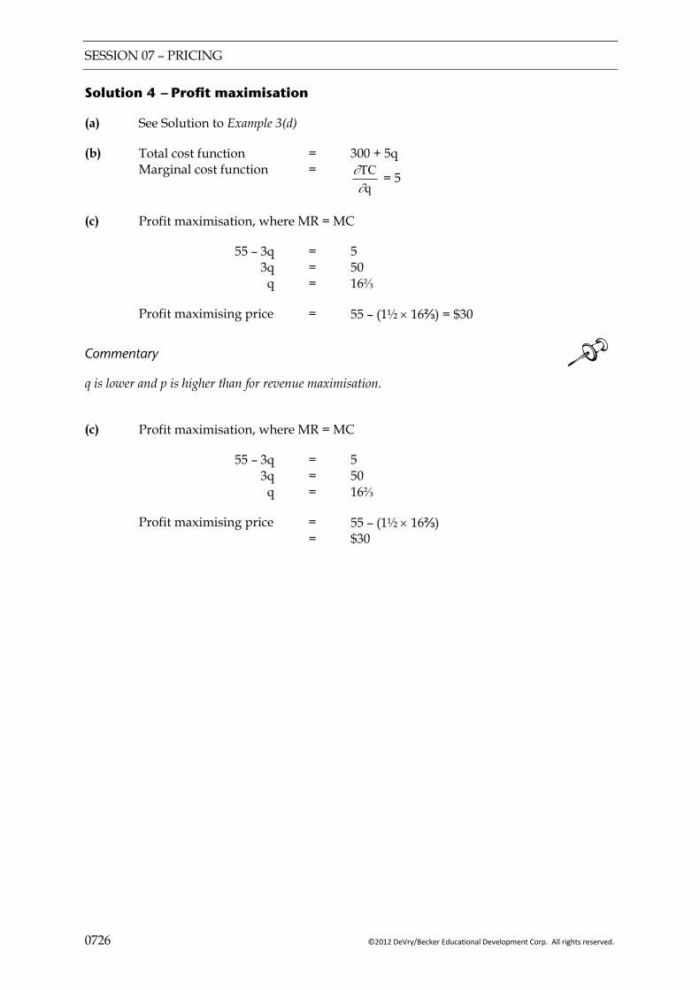
SESSION 07 – PRICING
0726 ©2012 DeVry/Becker Educational Development Corp. All rights reserved.
Solution 4 — Profit maximisation
(a) See Solution to Example 3(d)
(b) Total cost function = 300 + 5q Marginal cost function =
qTC∂∂ = 5
(c) Profit maximisation, where MR = MC
55 – 3q = 5 3q = 50 q = 16⅔
Profit maximising price = 55 – (1½ × 16⅔) = $30
Commentary q is lower and p is higher than for revenue maximisation.
(c) Profit maximisation, where MR = MC
55 – 3q = 5 3q = 50 q = 16⅔
Profit maximising price = 55 – (1½ × 16⅔) = $30
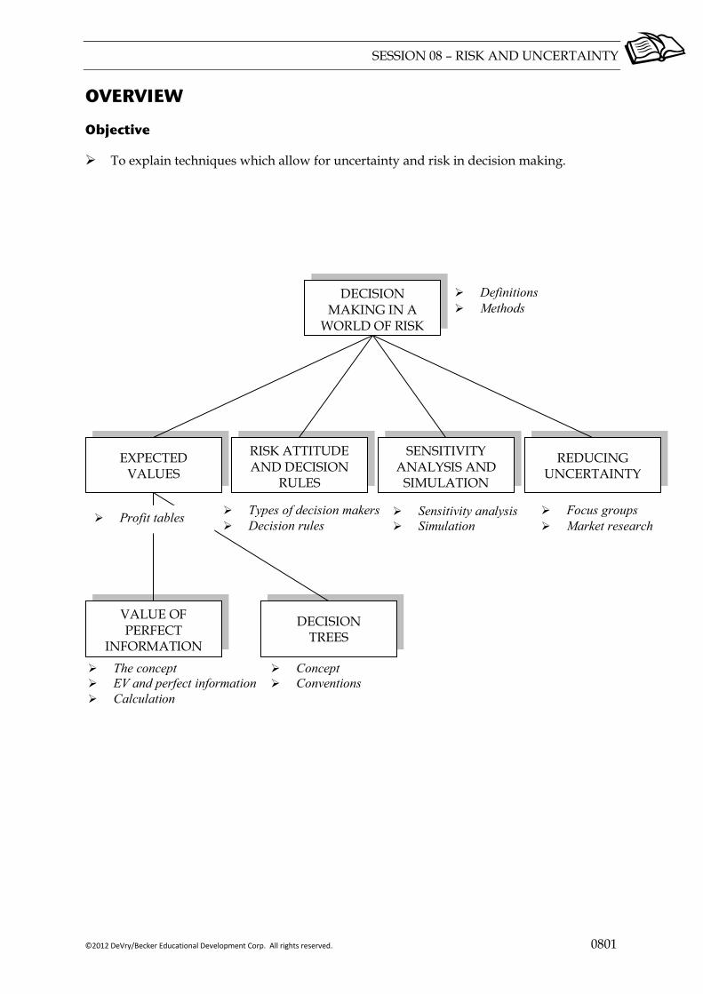
SESSION 08 – RISK AND UNCERTAINTY
©2012 DeVry/Becker Educational Development Corp. All rights reserved. 0801
OVERVIEW
Objective
To explain techniques which allow for uncertainty and risk in decision making.
EXPECTED VALUES
Definitions Methods
REDUCING UNCERTAINTY
DECISION MAKING IN A
WORLD OF RISK
SENSITIVITY ANALYSIS AND
SIMULATION
RISK ATTITUDE AND DECISION
RULES
Types of decision makers Decision rules
Sensitivity analysis Simulation
VALUE OF PERFECT
INFORMATION
DECISION TREES
Concept Conventions
Profit tables Focus groups Market research
The concept EV and perfect information Calculation
SESSION 08 – RISK AND UNCERTAINTY
0802 ©2012 DeVry/Becker Educational Development Corp. All rights reserved.
1 DECISION MAKING IN A WORLD OF RISK
1.1 Definitions
So far decision-making questions have assumed that the results of various courses of action are known with certainty. In the real world, this is seldom the case. Decisions often have to be made where various uncertain outcomes could result from the decision.
Definitions
Risk means that there are several possible outcomes, and these are known in advance, along with the related probability.
Uncertainty means that the potential outcomes of a decision are not known in advance. Clearly then associated probability cannot be known either.
1.2 Methods
There are several methods of dealing with risk in decision making. The methods that are dealt with in the syllabus for F5 are:
Expected value; Value of perfect information; Decision trees; Maximax; Maximin; Minimax regret.
The examiner also wants you to be aware of practical ways to deal with uncertainty.
2 EXPECTED VALUE (EV)
Expected value = weighted arithmetic mean of possible outcomes. = ∑ (x p(x))
Example 1
State of market Diminishing Static Expanding
Probability 0.4 0.3 0.3
Project 1 100 200 1,000
Project 2 0 500 600
Project 3 180 190 200
Payoffs represent the net present value of projects (in $000) under each market state.
Required:
Determine the best project based on expected value.
SESSION 08 – RISK AND UNCERTAINTY
©2012 DeVry/Becker Educational Development Corp. All rights reserved. 0803
Solution
Project 1 EV =
Project 2 EV =
Project 3 EV =
Advantages of EV
It reduces the information down to one number for each choice.
The idea of an average is easily understood.
Limitations of EV
The probabilities of the different possible outcomes may be difficult to estimate.
The average may not correspond to any of the possible outcomes.
Unless the same decision has to be made many times, the average will not be achieved; it is therefore unsuitable for decision making in “one off” situations.
The average gives no indication of the spread of possible results (i.e. it ignores risk).
2.1 Profit tables
A profit table (also referred to as a payoff matrix) shows all possible “payoffs” (NPVs, contribution, profits, etc) which may result from a decision maker’s chosen strategy. The data given in Example 1 is in the form of a payoff matrix.
Example 2
A baker pays 10¢ per cake and sells them for 30¢. At the end of a day any cakes not sold must be thrown away. On any particular day the level of demand follows the following probability distribution
No of cakes 20 40 60
Probability 0.3 0.5 0.2
Required:
(a) Construct a profit table to show the possible outcomes
(b) Calculate the daily order the baker should place in order to maximize the expected value of daily profits.
SESSION 08 – RISK AND UNCERTAINTY
0804 ©2012 DeVry/Becker Educational Development Corp. All rights reserved.
Solution
(a) Profit table
Order Demand 0.3 0.5 0.2 20 40 60
20
40
60
(b) EV if order 20 =
EV if order 40 =
EV if order 60 =
3 VALUE OF PERFECT INFORMATION
3.1 The concept
Imagine that, in a situation of uncertainty, it is possible to buy an accurate forecast that predicts with certainty what the uncertain variable is going to be each time a decision has to be made.
The value of perfect information is the maximum amount that a decision maker would be willing to pay for advance information to know which outcome will occur.
Illustration 1
If the baker in Example 2 could buy a daily forecast that would tell him how much demand would be each day, he would know exactly how many cakes to order. He would not buy too many cakes, but he would always have enough to meet demand. The maximum amount that he would be prepared to pay for such a report is the value of that perfect information.
3.2 EV with perfect information
Even if the baker were to order a daily forecast that would provide him with accurate data about daily sales, he still faces risk. The risk arises because although the daily forecasts will be accurate, the baker does not know what the forecasts will say for each day.
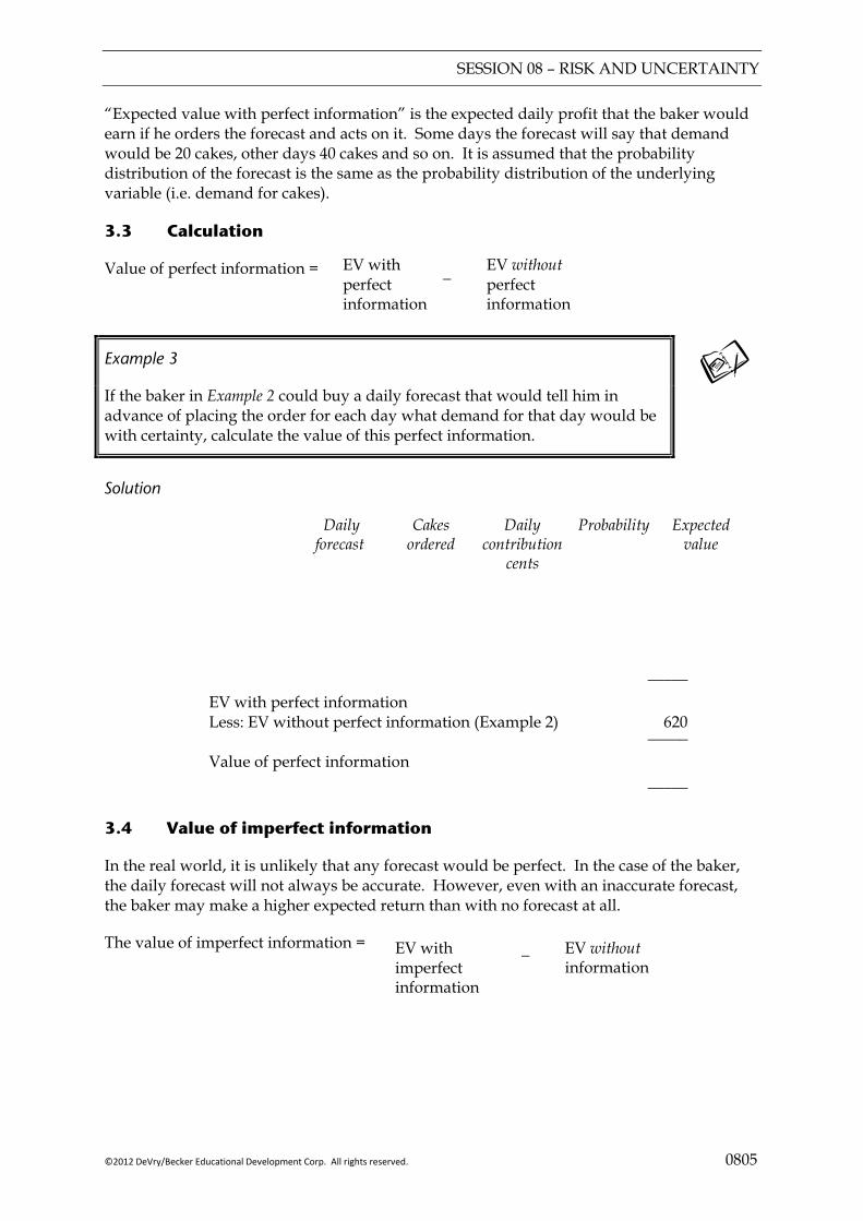
SESSION 08 – RISK AND UNCERTAINTY
©2012 DeVry/Becker Educational Development Corp. All rights reserved. 0805
“Expected value with perfect information” is the expected daily profit that the baker would earn if he orders the forecast and acts on it. Some days the forecast will say that demand would be 20 cakes, other days 40 cakes and so on. It is assumed that the probability distribution of the forecast is the same as the probability distribution of the underlying variable (i.e. demand for cakes).
3.3 Calculation
Value of perfect information =
Example 3
If the baker in Example 2 could buy a daily forecast that would tell him in advance of placing the order for each day what demand for that day would be with certainty, calculate the value of this perfect information.
Solution
Daily Cakes Daily Probability Expected forecast ordered contribution value cents _____
EV with perfect information Less: EV without perfect information (Example 2) 620 _____
Value of perfect information
_____
3.4 Value of imperfect information
In the real world, it is unlikely that any forecast would be perfect. In the case of the baker, the daily forecast will not always be accurate. However, even with an inaccurate forecast, the baker may make a higher expected return than with no forecast at all.
The value of imperfect information =
EV with perfect information
EV without perfect information
−
EV with imperfect information
− EV without information
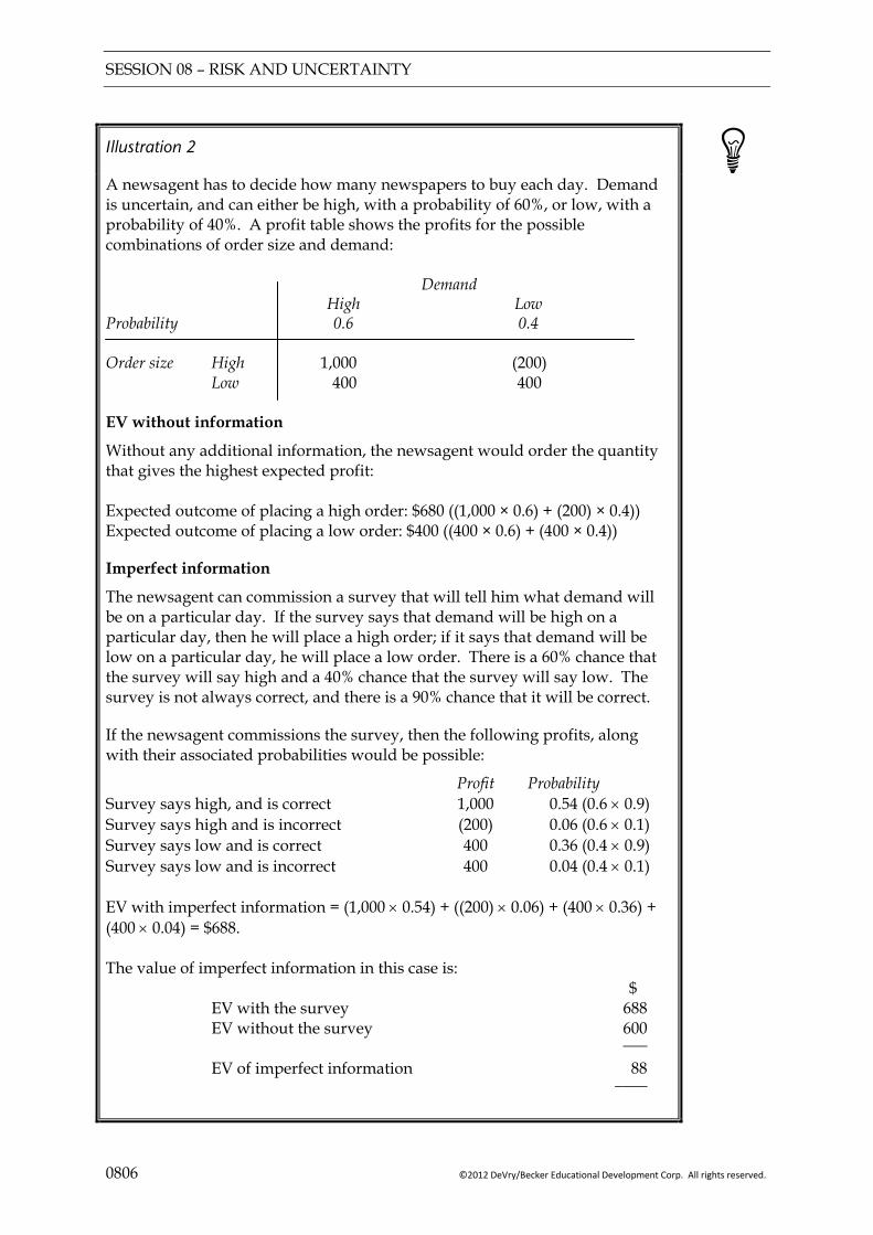
SESSION 08 – RISK AND UNCERTAINTY
0806 ©2012 DeVry/Becker Educational Development Corp. All rights reserved.
Illustration 2
A newsagent has to decide how many newspapers to buy each day. Demand is uncertain, and can either be high, with a probability of 60%, or low, with a probability of 40%. A profit table shows the profits for the possible combinations of order size and demand: Demand High Low Probability 0.6 0.4 Order size High 1,000 (200) Low 400 400 EV without information
Without any additional information, the newsagent would order the quantity that gives the highest expected profit: Expected outcome of placing a high order: $680 ((1,000 × 0.6) + (200) × 0.4)) Expected outcome of placing a low order: $400 ((400 × 0.6) + (400 × 0.4))
Imperfect information
The newsagent can commission a survey that will tell him what demand will be on a particular day. If the survey says that demand will be high on a particular day, then he will place a high order; if it says that demand will be low on a particular day, he will place a low order. There is a 60% chance that the survey will say high and a 40% chance that the survey will say low. The survey is not always correct, and there is a 90% chance that it will be correct.
If the newsagent commissions the survey, then the following profits, along with their associated probabilities would be possible:
Profit Probability Survey says high, and is correct 1,000 0.54 (0.6 × 0.9) Survey says high and is incorrect (200) 0.06 (0.6 × 0.1) Survey says low and is correct 400 0.36 (0.4 × 0.9) Survey says low and is incorrect 400 0.04 (0.4 × 0.1) EV with imperfect information = (1,000 × 0.54) + ((200) × 0.06) + (400 × 0.36) + (400 × 0.04) = $688. The value of imperfect information in this case is: $ EV with the survey 688 EV without the survey 600 ___ EV of imperfect information 88 ____
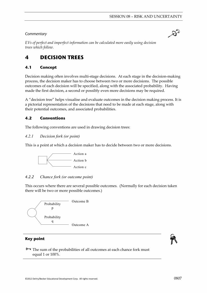
SESSION 08 – RISK AND UNCERTAINTY
©2012 DeVry/Becker Educational Development Corp. All rights reserved. 0807
Commentary EVs of perfect and imperfect information can be calculated more easily using decision trees which follow.
4 DECISION TREES
4.1 Concept
Decision making often involves multi-stage decisions. At each stage in the decision-making process, the decision maker has to choose between two or more decisions. The possible outcomes of each decision will be specified, along with the associated probability. Having made the first decision, a second or possibly even more decisions may be required.
A “decision tree” helps visualise and evaluate outcomes in the decision making process. It is a pictorial representation of the decisions that need to be made at each stage, along with their potential outcomes, and associated probabilities.
4.2 Conventions
The following conventions are used in drawing decision trees:
4.2.1 Decision fork (or point)
This is a point at which a decision maker has to decide between two or more decisions.
Action a
Action b
Action c
4.2.2 Chance fork (or outcome point)
This occurs where there are several possible outcomes. (Normally for each decision taken there will be two or more possible outcomes.)
Probabilityp
Probabilityq
Outcome B
Outcome A
Key point
The sum of the probabilities of all outcomes at each chance fork must equal 1 or 100%.
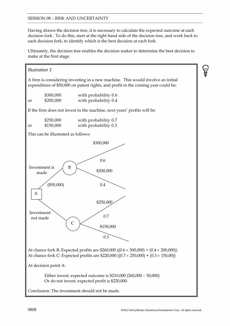
SESSION 08 – RISK AND UNCERTAINTY
0808 ©2012 DeVry/Becker Educational Development Corp. All rights reserved.
Having drawn the decision tree, it is necessary to calculate the expected outcome at each decision fork. To do this, start at the right hand side of the decision tree, and work back to each decision fork, to identify which is the best decision at each fork.
Ultimately, the decision tree enables the decision maker to determine the best decision to make at the first stage.
Illustration 3
A firm is considering investing in a new machine. This would involve an initial expenditure of $50,000 on patent rights, and profit in the coming year could be:
$300,000 with probability 0.6 or $200,000 with probability 0.4
If the firm does not invest in the machine, next years’ profits will be:
$250,000 with probability 0.7 or $150,000 with probability 0.3 This can be illustrated as follows:
At chance fork B: Expected profits are $260,000 ((0.6 × 300,000) + (0.4 × 200,000)) At chance fork C: Expected profits are $220,000 ((0.7 × 250,000) + (0.3 × 150,00))
At decision point A:
Either invest: expected outcome is $210,000 (260,000 − 50,000) Or do not invest: expected profit is $220,000.
Conclusion: The investment should not be made.
($50,000)
Investment is made
0.3
$250,000
A
Investment not made
B
C
$200,000
$150,000
0.6
0.4
$300,000
0.7

SESSION 08 – RISK AND UNCERTAINTY
©2012 DeVry/Becker Educational Development Corp. All rights reserved. 0809
Example 4
Slim Foods is considering launching a non-sugar snack bar into a new market. Although the company has not yet undertaken any market research the marketing director estimates that the product has a 60% chance of success and a 40% chance of failure in the market.
A market research company has offered to do some research in the new market prior to any decision being made to launch the product or not. Management believe that there is a 60% chance that the market research will recommend the launch, and a 40% chance that it will advise Slim Foods not to launch the product. The cost of the market research will be $30,000.
The market research company has admitted that their research findings do not always turn out to be as expected once the product has been launched. They advise that if they recommend the launch, there will be an 80% chance that the product will succeed and a 20% chance that it will fail. If they do not recommend the launch, there will be a 30% chance that the product would succeed if management were to launch it, and a 70% chance that it would fail.
In all cases, if the product succeeds, the present value of future profits from the product will be $10 million (excluding the market research costs), and if the product fails, the net present value of the loss would be $4.5 million (excluding the market research costs).
The directors of the company are trying to decide whether or not to accept the offer of the market research company, or to make a decision based only on the gut feel of the marketing director.
Required:
(a) Draw a decision tree to illustrate the possible decisions and their associated potential outcomes.
(b) Advise management how they should proceed.
(c) Calculate the value of the imperfect information provided by the market research company.
Solution

SESSION 08 – RISK AND UNCERTAINTY
0810 ©2012 DeVry/Becker Educational Development Corp. All rights reserved.
5 RISK ATTITUDE AND DECISION RULES
5.1 Three types of decision makers
“Risk seekers” are those who seek the maximum possible return regardless of the probability of it occurring. As optimists they consider the “best case” scenario.
“Risk neutral” are those who consider the most likely outcome.
“Risk averse” are those who make decisions based on the worst possible outcome.
5.2 Decision rules
MAXIMAX – Select the alternative with the maximum possible payoff (i.e. highest return under the best case scenario). The risk seeker’s (i.e. optimist’s) rule.
MAXIMIN – Select the alternative with the highest return under the worst case scenario. The pessimist’s rule (i.e. risk averse).
MINIMAX REGRET – Select the alternative with the lowest maximum “regret”. Regret is defined as the opportunity loss from having made the wrong decision.
Example 5
Using the payoff table in Example 1, determine which project would be chosen using the following decision rules:
(a) maximax; (b) maximin; (c) minimax regret.
Solution
(a)
(b)
(c) Opportunity loss table
Diminishing Static Expanding Maximum regret
Project 1
Project 2
Project 3
Conclusion:
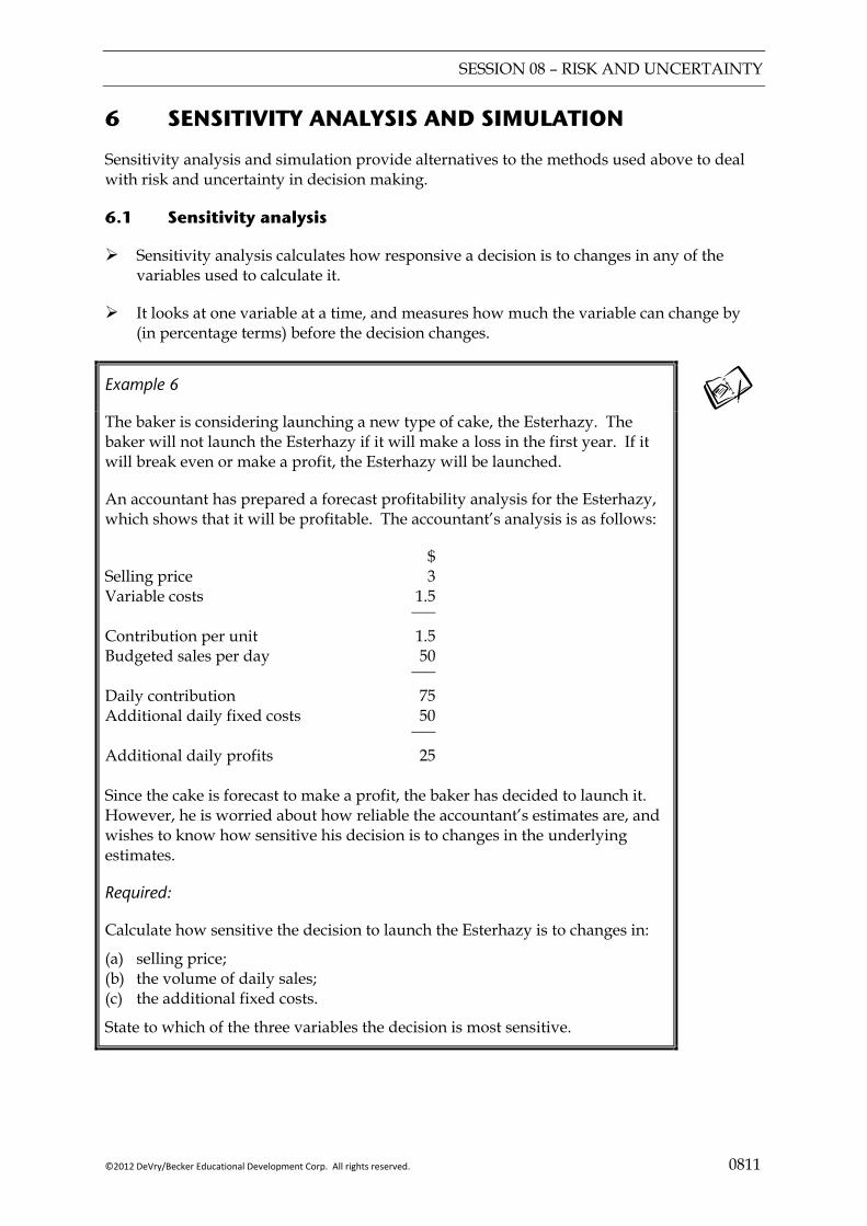
SESSION 08 – RISK AND UNCERTAINTY
©2012 DeVry/Becker Educational Development Corp. All rights reserved. 0811
6 SENSITIVITY ANALYSIS AND SIMULATION
Sensitivity analysis and simulation provide alternatives to the methods used above to deal with risk and uncertainty in decision making.
6.1 Sensitivity analysis
Sensitivity analysis calculates how responsive a decision is to changes in any of the variables used to calculate it.
It looks at one variable at a time, and measures how much the variable can change by (in percentage terms) before the decision changes.
Example 6
The baker is considering launching a new type of cake, the Esterhazy. The baker will not launch the Esterhazy if it will make a loss in the first year. If it will break even or make a profit, the Esterhazy will be launched.
An accountant has prepared a forecast profitability analysis for the Esterhazy, which shows that it will be profitable. The accountant’s analysis is as follows:
$ Selling price 3 Variable costs 1.5 ___
Contribution per unit 1.5 Budgeted sales per day 50 ___ Daily contribution 75 Additional daily fixed costs 50 ___ Additional daily profits 25 Since the cake is forecast to make a profit, the baker has decided to launch it. However, he is worried about how reliable the accountant’s estimates are, and wishes to know how sensitive his decision is to changes in the underlying estimates.
Required:
Calculate how sensitive the decision to launch the Esterhazy is to changes in:
(a) selling price; (b) the volume of daily sales; (c) the additional fixed costs.
State to which of the three variables the decision is most sensitive.

SESSION 08 – RISK AND UNCERTAINTY
0812 ©2012 DeVry/Becker Educational Development Corp. All rights reserved.
Solution
(a) Sensitivity to price
(b) Sensitivity to volume of daily sales
(c) Additional fixed costs
6.1.1 Advantages
It gives an idea of how sensitive the decision taken is to changes in any of the original estimates.
It can be readily adapted for use in spreadsheet packages.
6.1.2 Limitations
Although it can be adapted to deal with multi-variable changes, sensitivity is usually only used to examine what happens when one variable changes and others remain constant.
Without a computer it can be time consuming.
SESSION 08 – RISK AND UNCERTAINTY
©2012 DeVry/Becker Educational Development Corp. All rights reserved. 0813
6.2 Simulation
Definition
A mathematical model constructed to represent the operation of a real-life process or situation.
It is a technique which allows more than one variable to change at the same time.
Most real-life problems are complex in that there is more than one uncertain variable. Models can be generated which “simulate” the real world environment within which the decision must be made.
Illustration 4
A computer model could simulate the conditions which exist for the baker in Example 4. Each time the simulation is run (each trial) the model would randomly generate a selling price per unit, daily demand and daily fixed cost. The profit for the trial would then be calculated.
The simulation would be run many times. Based on the results of the simulation, a probability distribution of daily profit of the baker could be constructed.
Although a simulation is not likely to be used in such a simple situation (as alternative models are available), it may be the only suitable method of analysing more complex situations where there are many variables which could change.
One example of a mathematical model used in simulation is the “Monte Carlo” method.
Commentary This was the code name given to this method by the physicists who developed simulations to estimate the probability of success in nuclear weapon projects.
6.2.1 Stages
(1) Specify the major variables. (Excessive detail will over-complicate.)
(2) Specify the relationship between the variables.
(3) Attach probability distributions to each variable and assign random numbers to reflect the distribution.
(4) Simulate the environment by generating random numbers.
(5) Record the outcome of each simulation.
(6) Repeat simulation many times to obtain a probability distribution of the likely outcomes.
SESSION 08 – RISK AND UNCERTAINTY
0814 ©2012 DeVry/Becker Educational Development Corp. All rights reserved.
6.2.2 Advantages
It overcomes the limitations of sensitivity analysis by examining the effects of all possible combinations of variables and their realisations.
It therefore provides more information about the possible outcomes and their relative probabilities.
Commentary This helps in highlighting implausible assumptions and detecting bias (e.g. in optimistic assumptions).
It is useful for problems which cannot be solved analytically by other means.
6.2.3 Limitations
It is not a technique for making a decision, only for getting more information about the possible outcomes.
It can be very time consuming without a computer.
It could prove expensive in designing and running the simulation on a computer.
It relies on reliable estimates of the probability distributions of the underlying variables.
7 REDUCING UNCERTAINTY
7.1 Focus Groups
Much of the uncertainty that companies face in the real world relates to new products, and whether or not they will be successful. To reduce this uncertainty focus groups may be used prior to the launch of a new product.
A group of people is asked to give their opinion about a new product or service. The discussion takes place in an interactive environment where participants are free to give their opinions and discuss them with other members of the group.
Members of the group are chosen at random. Often they are approached by employees of the marketing organisation in the street and asked to participate.
Prior to the meeting, the members of the group may be screened to ensure they belong to the target market to which the product is aimed.
A moderator may be present to ease the discussion.
During the meeting itself, the participants may be observed, usually without their knowledge, by marketing professionals, who examine their body language, facial expressions and group behaviour.

SESSION 08 – RISK AND UNCERTAINTY
©2012 DeVry/Becker Educational Development Corp. All rights reserved. 0815
7.2 Market research
Market research is the systematic gathering of information about customers, competitors and the market. The type of information gathered in market research seeks to answer the following types of question:
Who are the customers? Where are they located? What quantity and quality do they want? What is the best time to sell? What is the long-term price? Who are the competitors?
Market research can be used to help companies make decisions about the development and marketing of new products.
The earlier the market research is conducted in the development of a product, the better, from a risk point of view.
Market research can be based on primary or secondary data. Primary data means that the company collects its own original data, for example by conducting interviews. Secondary data means that already published data is used, such as published statistics.
Key points
Various techniques can be used to make decisions in situations of uncertainty.
EV analysis involves choosing the outcome with the highest expected outcome. This is based on probabilities, and is an average value. It may not be appropriate for one off decisions.
Value of perfect information shows the maximum amount that a company would be prepared to pay for an accurate forecast of the uncertain variables it faces. It is defined as:
EV with perfect information (the forecast) less EV without the forecast.
Decision trees may be used to document multi-stage decisions with various potential outcomes at each stage.
Maximax decision making involves choosing the option with the highest potential outcome. Maximax decision makers are risk seekers.
Maximin decision makers are pessimists, who assume that only the worst outcome will occur. They therefore select the option where the worst outcome is higher.
In the real world, much of the risk that commercial organisations face comes from new products. Such risk can be reduced by focus groups or other forms of market research.
SESSION 08 – RISK AND UNCERTAINTY
0816 ©2012 DeVry/Becker Educational Development Corp. All rights reserved.
FOCUS
You should now be able to:
explain the use of simulation, expected values and sensitivity;
apply expected values and sensitivity to decision-making problems;
apply the techniques of maximax, maximin and minimax regret to decision-making problems including the production of profit tables;
draw a decision tree and use it to solve a multi-stage decision program;
calculate the value of perfect information;
suggest research techniques to reduce uncertainty (e.g. focus groups, market research).
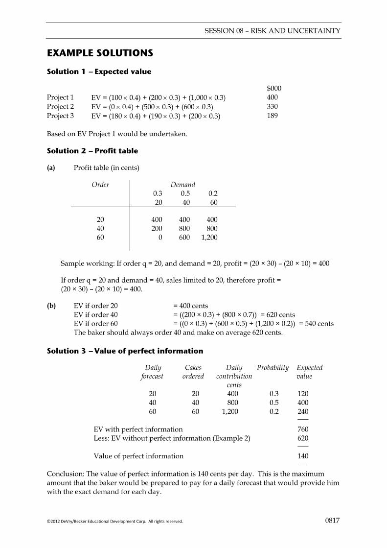
SESSION 08 – RISK AND UNCERTAINTY
©2012 DeVry/Becker Educational Development Corp. All rights reserved. 0817
EXAMPLE SOLUTIONS
Solution 1 — Expected value
$000 Project 1 EV = (100 × 0.4) + (200 × 0.3) + (1,000 × 0.3) 400 Project 2 EV = (0 × 0.4) + (500 × 0.3) + (600 × 0.3) 330 Project 3 EV = (180 × 0.4) + (190 × 0.3) + (200 × 0.3) 189 Based on EV Project 1 would be undertaken.
Solution 2 — Profit table
(a) Profit table (in cents)
Order Demand 0.3 0.5 0.2 20 40 60
20 40 60
400 400 400 200 800 800 0 600 1,200
Sample working: If order q = 20, and demand = 20, profit = (20 × 30) – (20 × 10) = 400
If order q = 20 and demand = 40, sales limited to 20, therefore profit = (20 × 30) – (20 × 10) = 400.
(b) EV if order 20 = 400 cents EV if order 40 = ((200 × 0.3) + (800 × 0.7)) = 620 cents EV if order 60 = ((0 × 0.3) + (600 × 0.5) + (1,200 × 0.2)) = 540 cents The baker should always order 40 and make on average 620 cents. Solution 3 — Value of perfect information
Daily Cakes Daily Probability Expected forecast ordered contribution value cents 20 20 400 0.3 120 40 40 800 0.5 400 60 60 1,200 0.2 240 ___
EV with perfect information 760 Less: EV without perfect information (Example 2) 620 ___
Value of perfect information 140 ___
Conclusion: The value of perfect information is 140 cents per day. This is the maximum amount that the baker would be prepared to pay for a daily forecast that would provide him with the exact demand for each day.

SESSION 08 – RISK AND UNCERTAINTY
0818 ©2012 DeVry/Becker Educational Development Corp. All rights reserved.
Solution 4 — Decision trees
(a) Decision tree
A
Market research
No research
C
Launch
Success0.6
0.4
($30,000)
Do not launch
Fail
0.8
Fail
0.2 ($4.5 million)
Success$10 million
$0
Success$10 million
($4.5 million)
$0
D
Launch
Do not launch
E
Launch
Do not launch
Launchrecommended
Launch not recommended
0.6
0.4
B
F
G
H 0.3
0.7
Fail
$0
$10 million
($4.5 million)
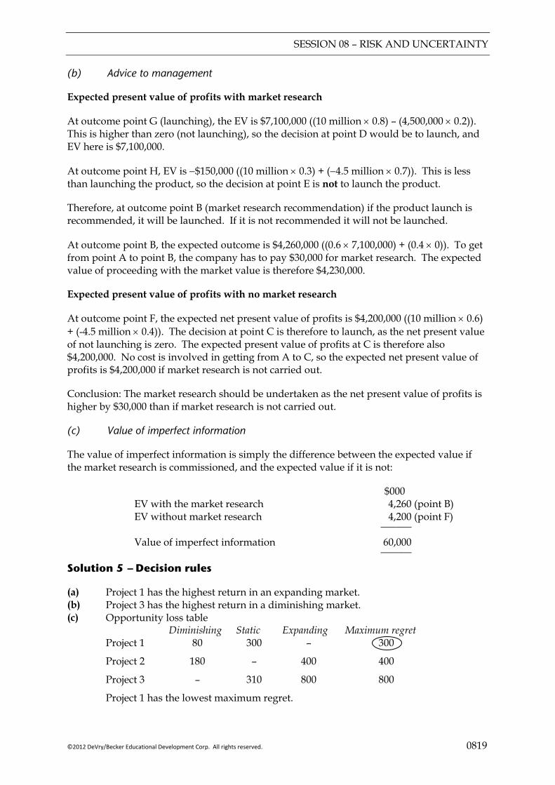
SESSION 08 – RISK AND UNCERTAINTY
©2012 DeVry/Becker Educational Development Corp. All rights reserved. 0819
(b) Advice to management
Expected present value of profits with market research
At outcome point G (launching), the EV is $7,100,000 ((10 million × 0.8) – (4,500,000 × 0.2)). This is higher than zero (not launching), so the decision at point D would be to launch, and EV here is $7,100,000.
At outcome point H, EV is −$150,000 ((10 million × 0.3) + (−4.5 million × 0.7)). This is less than launching the product, so the decision at point E is not to launch the product.
Therefore, at outcome point B (market research recommendation) if the product launch is recommended, it will be launched. If it is not recommended it will not be launched.
At outcome point B, the expected outcome is $4,260,000 ((0.6 × 7,100,000) + (0.4 × 0)). To get from point A to point B, the company has to pay $30,000 for market research. The expected value of proceeding with the market value is therefore $4,230,000.
Expected present value of profits with no market research
At outcome point F, the expected net present value of profits is $4,200,000 ((10 million × 0.6) + (-4.5 million × 0.4)). The decision at point C is therefore to launch, as the net present value of not launching is zero. The expected present value of profits at C is therefore also $4,200,000. No cost is involved in getting from A to C, so the expected net present value of profits is $4,200,000 if market research is not carried out.
Conclusion: The market research should be undertaken as the net present value of profits is higher by $30,000 than if market research is not carried out.
(c) Value of imperfect information
The value of imperfect information is simply the difference between the expected value if the market research is commissioned, and the expected value if it is not:
$000 EV with the market research 4,260 (point B) EV without market research 4,200 (point F) ______
Value of imperfect information 60,000 ______
Solution 5 — Decision rules
(a) Project 1 has the highest return in an expanding market. (b) Project 3 has the highest return in a diminishing market. (c) Opportunity loss table Diminishing Static Expanding Maximum regret Project 1 80 300 – 300
Project 2 180 – 400 400
Project 3 – 310 800 800
Project 1 has the lowest maximum regret.
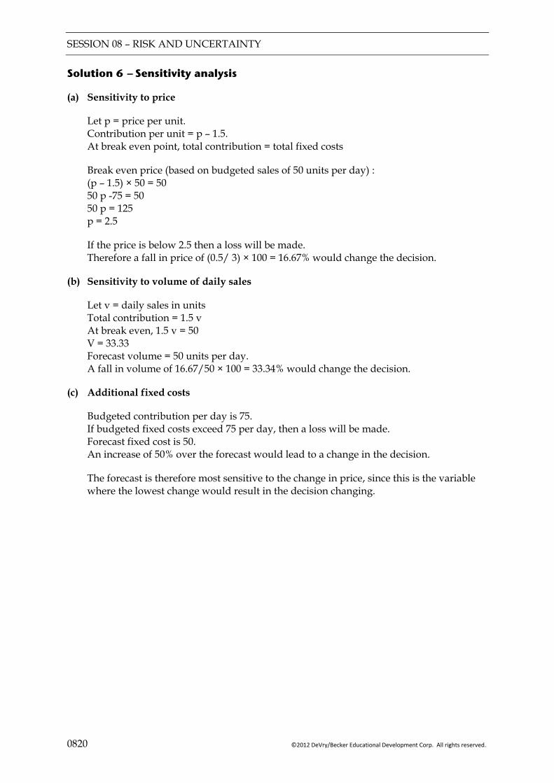
SESSION 08 – RISK AND UNCERTAINTY
0820 ©2012 DeVry/Becker Educational Development Corp. All rights reserved.
Solution 6 — Sensitivity analysis
(a) Sensitivity to price
Let p = price per unit. Contribution per unit = p – 1.5. At break even point, total contribution = total fixed costs
Break even price (based on budgeted sales of 50 units per day) : (p – 1.5) × 50 = 50 50 p -75 = 50 50 p = 125 p = 2.5
If the price is below 2.5 then a loss will be made. Therefore a fall in price of (0.5/ 3) × 100 = 16.67% would change the decision.
(b) Sensitivity to volume of daily sales
Let v = daily sales in units Total contribution = 1.5 v At break even, 1.5 v = 50 V = 33.33 Forecast volume = 50 units per day. A fall in volume of 16.67/50 × 100 = 33.34% would change the decision.
(c) Additional fixed costs
Budgeted contribution per day is 75. If budgeted fixed costs exceed 75 per day, then a loss will be made. Forecast fixed cost is 50. An increase of 50% over the forecast would lead to a change in the decision.
The forecast is therefore most sensitive to the change in price, since this is the variable where the lowest change would result in the decision changing.

SESSION 09 – BUDGETING
©2012 DeVry/Becker Educational Development Corp. All rights reserved. 0901
OVERVIEW
Objective
To describe, illustrate and comment on the planning and control uses of budgeting.
OBJECTIVES OF A BUDGETARY
CONTROL SYSTEM
BEHAVIOURAL ASPECTS OF BUDGETING
CORPORATE AND DIVISIONAL OBJECTIVES
CONFLICTING OBJECTIVES
Introduction Objectives
Potential conflicts Corporate objectives Divisional objectives How reconciled
Potential for conflict
DIFFERENT TYPES OF BUDGETARY
SYSTEMS
INFORMATION USED
Introduction Top-down vs bottom-up Rolling budgets Incremental Budgeting Zero base budgeting (ZBB) Activity based budgeting (ABB) Feedback and feed forward control
PERFORMANCE HIERARCHY
Long term planning Mission Corporate objectives Unit objectives Setting strategies Role of budgeting in long term
planning
Quality aspects Sources of data and information
DIFFICULTIES OF CHANGING
Traditional approaches to budgeting
Difficulties
UNCERTAINTY IN THE ENVIRONMENT
Forecasting Flexible budgets Flexed budgets
Factors which influence behaviour Hopwood’s management styles Setting the level of difficulty Standards Benefits and difficulties of
participation
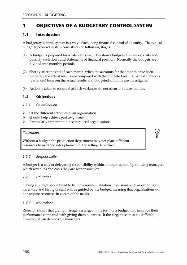
SESSION 09 – BUDGETING
0902 ©2012 DeVry/Becker Educational Development Corp. All rights reserved.
1 OBJECTIVES OF A BUDGETARY CONTROL SYSTEM
1.1 Introduction
A budgetary control system is a way of achieving financial control of an entity. The typical budgetary control system consists of the following stages:
(1) A budget is prepared for a calendar year. This shows budgeted revenues, costs and possibly cash flows and statements of financial position. Normally the budgets are divided into monthly periods.
(2) Shortly after the end of each month, when the accounts for that month have been prepared, the actual results are compared with the budgeted results. Any differences (variances) between the actual results and budgeted amounts are investigated.
(3) Action is taken to ensure that such variances do not occur in future months.
1.2 Objectives
1.2.1 Co-ordination
Of the different activities of an organisation. Should help achieve goal congruence. Particularly important in decentralised organisations.
Illustration 1
Without a budget, the production department may not plan sufficient resources to meet the sales planned by the selling department.
1.2.2 Responsibility
A budget is a way of delegating responsibility within an organisation, by showing managers which revenues and costs they are responsible for.
1.2.3 Utilisation
Having a budget should lead to better resource utilisation. Decisions such as ordering of inventory and hiring of staff will be guided by the budget, meaning that organisations do not acquire resources in excess of the needs. 1.2.4 Motivation
Research shows that giving managers a target in the form of a budget may improve their performance compared with giving them no target. If the target becomes too difficult, however, it can demotivate managers.
SESSION 09 – BUDGETING
©2012 DeVry/Becker Educational Development Corp. All rights reserved. 0903
1.2.5 Planning
Budgets are a financial plan. Requiring managers to prepare budgets forces them to think about the budget period. It makes them consider what conditions may exist and how they will respond to them. This should lead to better decision making than simply “taking each day as it comes”. Budgets cover a short-term time frame, typically one year. Most organisations have a long-term plan too. The budget should be consistent with the long-term plan as it shows, in detail, how the budgeted period will contribute towards the longer-term objectives. 1.2.6 Evaluation
Managers’ performance is likely to be evaluated, at least in part, by how they perform against the budget they are given. In some organisations, managers may receive bonuses based on how they perform relative to the budget. Promotions may also depend on this. In such situations, managers will be extremely keen to ensure that they achieve the budget. 1.2.7 Telling
Budgets are a means by which superiors communicate their expectations of the managers below them.
Commentary The first letter of each of the objectives of budgeting spells the word “Crumpet”. This may help you to remember the objectives of budgeting.
2 CORPORATE AND DIVISIONAL OBJECTIVES
2.1 Goal congruence
A budgetary control system should help achieve “goal congruence” by motivating the divisional managers to behave in a way that helps the organisation to achieve its corporate objectives. However, budgets may lead to conflicts between the objectives of an organisation and the division.
2.2 Corporate objectives
Corporate objectives are objectives that apply to the whole organisation.
They are usually formulated by the board of directors of a company.
A common assumption for commercial organisations is that the primary objective is to maximise the wealth of shareholders.
Corporate objectives may also focus on other areas, such as achieving a certain share of the market, behaving in an ethical fashion, and providing satisfactory working conditions for the staff.
SESSION 09 – BUDGETING
0904 ©2012 DeVry/Becker Educational Development Corp. All rights reserved.
2.3 Divisional objectives
The objectives of the management of a division are likely to focus on achieving the targets that have been set for the managers, particularly if promotion or bonuses depend on these.
If the targets are based on budgets, management of divisions are likely to spend energy ensuring that they achieve their budgets.
2.4 Potential conflicts
While it may appear at first sight that managers trying to achieve their targets should not conflict with corporate objectives, there may be conflicts if:
If the performance measures set are not consistent with the corporate objectives. This may be the case if the results that are required to achieve the corporate objectives can only be partially specified.
There is a risk that performance measures will only focus on things that can be measured, such as revenues and costs, while ignoring other important objectives that are less easy to measure such as quality and staff morale.
Performance measures may encourage a short-term view among managers, while corporate objective may take a longer-term view.
Goal incongruence is the term used to describe the situation where the objectives of divisions or managers are not the same as the objectives of the organisation.
Illustration 2
The corporate objectives of a consultancy company are likely to include recruiting and retaining high calibre staff.
If divisional managers are judged on whether or not they achieve budgeted profits, those managers may take actions such as freezing salaries, or reducing headcount. This may help to achieve the budgeted profits. However, it may mean that the better employees leave the company to find higher paid jobs elsewhere. Thus the objectives of the divisional managers are conflicting with the corporate objectives.
2.5 How to reconcile corporate and divisional objectives
The following steps can be taken to try to reconcile corporate and divisional objectives:
Use a wider range of performance measures rather than relying only on budget targets. (See Sessions 15 & 16 for the use of financial and non-financial performance measures.)
Use performance measures that are consistent with the corporate objectives, such as residual income, discussed in the session on divisional performance evaluation.
Enable the divisional managers to participate in the setting of their own targets so they have faith in them.
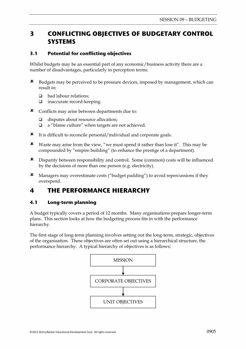
SESSION 09 – BUDGETING
©2012 DeVry/Becker Educational Development Corp. All rights reserved. 0905
3 CONFLICTING OBJECTIVES OF BUDGETARY CONTROL SYSTEMS
3.1 Potential for conflicting objectives
Whilst budgets may be an essential part of any economic/business activity there are a number of disadvantages, particularly in perception terms.
Budgets may be perceived to be pressure devices, imposed by management, which can result in:
bad labour relations; inaccurate record-keeping.
Conflicts may arise between departments due to:
disputes about resource allocation; a “blame culture” when targets are not achieved.
It is difficult to reconcile personal/individual and corporate goals.
Waste may arise from the view, “we must spend it rather than lose it”. This may be compounded by “empire building” (to enhance the prestige of a department).
Disparity between responsibility and control. Some (common) costs will be influenced by the decisions of more than one person (e.g. electricity).
Managers may overestimate costs (“budget padding”) to avoid repercussions if they overspend.
4 THE PERFORMANCE HIERARCHY
4.1 Long-term planning
A budget typically covers a period of 12 months. Many organisations prepare longer-term plans. This section looks at how the budgeting process fits in with the performance hierarchy.
The first stage of long-term planning involves setting out the long-term, strategic, objectives of the organisation. These objectives are often set out using a hierarchical structure, the performance hierarchy. A typical hierarchy of objectives is as follows:
MISSION
CORPORATE OBJECTIVES
UNIT OBJECTIVES
SESSION 09 – BUDGETING
0906 ©2012 DeVry/Becker Educational Development Corp. All rights reserved.
4.2 Mission
The mission of an organisation can be described as the reason for the organisation’s existence. In the case of commercial organisations, the mission is normally to maximise the wealth of shareholders.
Non-profit organisations’ missions will not normally be to maximise the wealth of shareholders, but will be based on achieving some other aim. The mission of the environmental group Greenpeace, for example is set out in a mission statement. This includes the following statement: “Greenpeace is an independent global campaigning organisation that acts to change attitudes and behaviour, to protect and conserve the environment and to promote peace.”
4.3 Corporate objectives
Whether or not an organisation is achieving its objectives is often a matter of opinion, as it is not normally set out in quantifiable terms. Corporate objectives are more concrete and set out what the organisation must do in order to achieve its mission. Corporate objectives are specific and quantifiable. Examples of corporate objectives are as follows:
To increase revenues by 10% per annum
To increase dividends by 5% per year.
To reduce global emissions of carbon gasses by 10% by the year 2015.
4.4 Unit objectives
Having set objectives for the organisation as a whole (Corporate objectives), objectives may then be set for each business unit. These should be consistent with the Corporate Objectives.
4.5 Setting strategies
Having established the objectives of the organisation, possibly using the performance hierarchy approach, organisations need to determine what actions they will take to achieve those objectives. These strategies may be set out in a long-term plan.
4.6 Role of budgeting in long-term planning
A budget is concerned with implementing the long-term plan for the budget period. The budget will be more detailed than the long-term plan, and shows essentially how the budget period will contribute towards the long-term plan.
4.6.1 Diagram
The following diagram summarises the discussion above about how budgetary systems fit within the performance hierarchy:

SESSION 09 – BUDGETING
©2012 DeVry/Becker Educational Development Corp. All rights reserved. 0907
Examples • Sales volume maximisation • Sales revenue maximisation • Profit maximisation
Establish long term corporate
Long term plannin
Produce a specific (but rolling) corporate plan
Produce sales forecasts which would enable plans to be
Functional Sales Production Material usage Materials purchases Labour Fixed overhead
Financial Capital expenditure Cash
MASTER BUDGET
BOARD APPROVAL
Redraft long term plan in the form of annual budgets
Budget officer
+
Budget committee
Compare budgets with actual performance: calculate variances
Take action on variances − improve performance − revise plans
Short term planning and budgetary control
5 DIFFERENT TYPES OF BUDGETARY SYSTEMS
5.1 Introduction
A number of different approaches to the preparation of budgets have evolved. It is important to understand what these approaches are, and to appreciate which would be appropriate for different types of organisation. The approaches mentioned in the ACCA Study Guide are as follows:
Top-down; Bottom-up; Rolling budgets; Zero-based budgeting (ZBB); Activity-based budgeting (ABB); Incremental; Feed-forward control.
SESSION 09 – BUDGETING
0908 ©2012 DeVry/Becker Educational Development Corp. All rights reserved.
5.2 Top-down vs bottom-up
Definition
Top-down budgeting means that budgets are prepared by senior management.
Bottom-up means that managers participate in the preparation of their department’s budget.
In practice top-down budgets are often prepared through a finance department.
Bottom-up budgeting usually means that managers prepare the budgets for the department they are responsible for. These budgets are then approved by senior management (usually after some negotiation and discussion).
Example 1
Suggest four advantages of top-down budgeting and four advantages of bottom-up budgeting.
Solution
Top-down
Bottom-up

SESSION 09 – BUDGETING
©2012 DeVry/Becker Educational Development Corp. All rights reserved. 0909
5.2.2 Appropriateness of top-down and bottom-up budgeting
Whether top-down or bottom-up budgeting is more appropriate for a particular organisation depends on the nature and talents of the managers.
Douglas McGregor developed two theories of human behaviour at work:
Theory X − people dislike work; − people dislike responsibility; − they are only motivated by money; − they must be told what to do.
Theory Y − people seek responsibility; − they want to participate in decision making.
Some organisations employ theory X managers, while other organisations employ theory Y managers. The type of managers employed will determine what method of budgetary control is more appropriate:
Employee type X Y Motivated by Money Many factors Dues participation increase motivation? No Yes Management style Authoritarian Participative approach approach Budgeting style TOP DOWN BOTTOM UP
5.3 Rolling Budgets (Rolling forecasts)
Definition
A rolling budget is a system of budgeting where the budget is continuously updated. The budget horizon (typically one year) is kept constant by adding another month (or quarter) to the end of the budgeted period as each month (or quarter) expires.
SESSION 09 – BUDGETING
0910 ©2012 DeVry/Becker Educational Development Corp. All rights reserved.
Illustration 3
A budget is prepared for the year 2012.
At the end of January 2012, the actual performance for the month of January is compared against the budget. Based on this comparison, it may be decided that the budgets for the period 1 Feb to 31 Dec 2012 should be changed to reflect changes in external factors. Once this has been done, a budget is also prepared for January 2013. The new budget therefore covers the period from 1 February 2012 to 31 January 2013.
5.3.1 Usefulness of rolling budgets
The budget is always updated to reflect external changes. It is therefore more relevant and more valid for comparison against actual performance.
There will always be a budget for the next twelve months. This can be useful for planning things such as cash flows.
Managers will be more motivated as the budget is more realistic, since it will be updated to take account of changes that occur that are outside of their control.
5.3.2 Problems with rolling budgets
Time consuming Budgets may be changed to hide operational inefficiencies Not necessary in a stable environment
5.3.3 Appropriateness of rolling budgets
Rolling budgets are likely to be more appropriate in industries that are dynamic, where external changes can lead to the original budget becoming out of date quickly. In stable industries, little benefit may be obtained by continuously updating the budget, so a rolling budget may be less useful.
Example 2
For organisations in each of the following industries, discuss whether rolling budgets would be appropriate or not:
A food retailer;
A developer of handheld computer devices and mobile telephones;
An airline;
An advertising agency;
A retail bank.
SESSION 09 – BUDGETING
©2012 DeVry/Becker Educational Development Corp. All rights reserved. 0911
5.4 Incremental budgeting
5.4.1 Use of historic data
An incremental budget is a budget prepared using a previous period’s budget or actual performance as a basis with incremental amounts added for the new budget period. The allocation of resources is based upon allocations in the previous period. It is not generally recommended as it fails to take into account changing circumstances. Also it encourages a “spend it or lose” mentality as spending the budget is likely to ensure a reasonable allocation in the next period.
5.4.2 Usefulness of incremental budgeting
The budget is stable and change is gradual. Managers can operate their departments on a consistent basis. The system is relatively simple to operate and easy to understand. Conflicts should be avoided if departments can be seen to be treated similarly. Co-ordination between budgets is easier to achieve. The impact of change can be seen quickly.
5.4.3 Problems with incremental budgeting
Assumes activities and methods of working will continue in the same way.
No incentive for developing new ideas.
No incentives to reduce costs.
Encourages “spend it or lose” mentality so that the budget is maintained next year.
The budget may become out of date and no longer relate to the level of activity or type of work being carried out.
The priority for resources may have changed since the budgets were set originally.
There may be budgetary “slack” built into the budget, which is never reviewed.
Commentary Managers may have overestimated their requirements in the past to obtain a budget which is easier to work to, and which will allow them to achieve favourable results.
5.5 Zero-base budgeting (ZBB)
5.5.1 Weakness of incremental budgeting
When a budgeting system has been in operation for some time, there is a tendency for next year’s budget to be justified by reference to the actual levels currently being achieved. However, the analysis process should take into account all changes which should affect the future activities of the organisation.
SESSION 09 – BUDGETING
0912 ©2012 DeVry/Becker Educational Development Corp. All rights reserved.
Even using such an analytical base, some organisations find that historical comparisons, and particularly the current level of constraints on resources, can inhibit innovative changes in budgets. This can severely handicap an organisation because the budget should be the first year of the long-term strategic plan. If changes are not started in the budget period, it will be more difficult for the organisation to make the progress necessary to achieve long-term objectives.
One way of breaking out of this “cyclical” budgeting problem is to go back to basics and develop the budget from an assumption of no existing resources (i.e. a “zero base”). Using this bases all resources have to be justified and the chosen way of achieving any specified objectives has to be compared with the alternatives. For example, in considering budgeted sales, the current existing sales force would be ignored, and the optimum means of achieving the sales objectives in a particular market for a particular product or service would be developed. This might not include any of the sales force, or a different-sized team, and the company then has to plan how to implement this new strategy.
5.5.2 Features of ZBB
Start each budget period afresh-not based on historical data.
Budgets are zero unless managers make the case for resources-the relevant manager must justify the whole of the budget allocation.
Each activity is questioned as if it were new before any resources are allocated to it. A decision package is prepared for each activity, stating the total costs and revenues associated with the activity, and some narrative explaining the benefits to the organisation of performing the activity.
A budgeting committee will then review all decision packages and decide which packages should be accepted and which rejected.
The final budget is prepared by consolidating the costs and revenues associated with the decision packages that have been accepted.
5.5.3 Usefulness of ZBB
Forces budget setters to examine every item. Allocation of resources linked to results and needs. Develops a questioning attitude. Wastage and budget slack should be eliminated. Prevents budgets “creeping” based on previous year’s figures with a % add-on. Encourages managers to look for alternatives.
5.5.4 Problems with ZBB
It a complex and time-consuming process. Short-term benefits may be emphasised to the detriment of long-term planning. Internal politics can result in annual conflicts over budget allocation.
SESSION 09 – BUDGETING
©2012 DeVry/Becker Educational Development Corp. All rights reserved. 0913
Commentary The main problem with ZBB is the huge amount of managerial time needed to carry out the exercise. Hence, the full process may be carried out only every five years (say). However, this could result in a business almost grinding to a halt during the budgeting process. An alternative approach is to look in depth at one area of the business each year on a rolling basis so that each area prepares a ZBB every five years.
5.5.5 When ZBB is appropriate
ZBB is most appropriate in organisations that have a high portion of discretionary costs. A discretionary cost means that managers have some choice as to the amount they spend on a particular item. Discretionary costs normally include items such as research and development, training and advertising. Expenditure on such items may be reduced without the organisation ceasing to function; however such expenditure does bring benefits. The use of ZBB enables organisations to reassess how much they spend on such discretionary items.
Organisations that enjoy few such discretionary items of expenditure would not gain so much from introducing ZBB.
Example 3
Discuss whether or not zero-based budgeting should be used in preparing the budgets of central governments.
Solution
5.6 Activity-based budgeting (ABB)
5.6.1 Principles of ABB
Most budgeting techniques assume that costs vary with the level of output. However, costs of support activities do not necessarily depend on the number of units produced or sold (see Session 2). For these types of cost, a more sophisticated type of budgeting is called for.
ABB follows principles of activity based costing (ABC) “in reverse”. Having decided how many units to produce and sell, the organisation then needs to define the cost of the activities required to produce them. These depend on the drivers identified for each activity. A typical ABB exercise may follow the following steps:
(1) Estimate the expected output (units) for each product.
(2) Identify the number of units of each activity that will be required to produce the output. This is based on knowledge of the relationships between the output and the activities that are required to be performed to product the output.

SESSION 09 – BUDGETING
0914 ©2012 DeVry/Becker Educational Development Corp. All rights reserved.
(3) Determine the resources needed to perform the activities required. This is based on knowledge of the drivers – the factors that influence the price of the activities.
(4) If the current commitment of resources is such that too many or too few resources exist to perform the activities required in (3)d, then adjust accordingly.
Illustration 4
Alex uses activity based costing and wishes to adopt an activity-based approach to budgeting.
Having estimated the total budgeted sales for the next financial year (Step 1 above), Alex has identified that one of the activities needed for to support the budgeted sales is “Processing sales orders”. Alex has identified that 2,800 orders will be received next year (Step 2).
One of the resources needed for processing orders is staff. Each member of staff in the Sales Order department can handle 60 orders per month, or 720 order per year. Since Alex expects 2,800 orders next year, the company will need 3.88, or 4 members of staff. (Step 3).
Currently Alex employs 6 members of staff in the Sales Order Processing department. Alex should consider relocating two members of staff to other departments.
Activity-based budgets are performed by repeating the steps above for all activities in an organisation and preparing a total budget. Organisations often use a matrix approach to such budgets, with a column for each activity, and a line for each type of expenditure.
Example 4
Suggest two advantages and two disadvantages of using activity-based budgeting.
Solution
SESSION 09 – BUDGETING
©2012 DeVry/Becker Educational Development Corp. All rights reserved. 0915
5.6.2 Appropriateness of ABB
ABB is a complex method. It is likely to only be used in large companies that have the resources to implement such an approach. It is most appropriate in situations where:
The organisation has large volume of overheads. There are several different activities that the overheads relate to. The organisation has many products with differing production times and methods.
5.7 Feedback and feed-forward Control
5.7.1 Feedback control
A feedback control system is a system where outputs are monitored against a pre-determined standard, and if there are any deviations from the standard, action is taken to remedy these. The feedback is the information concerning the difference between the actual output and the desired output.
A budgetary control system is an example of a feedback control system. Each period, the actual results are compared against the budget. If the budget was not achieved, then action can be taken to correct the factor that caused the budget to be missed.
5.7.2 Feed-forward control
The major problem with feedback control systems is that by the time the feedback is received, it is too late to take action to correct the deviation for the period under review. If actual costs are higher than budget for example, action can be taken that will stop the same deviation occurring in future periods. The current period however is already history, so no action can be taken to change that.
In feed-forward control systems, predicted future results are compared against the desired outcome. If it appears that the desired outcome will not be achieved based on the current prediction, action can be taken now, so that the desired outcome is achieved.
Illustration 5
Alpha operates in a business that is not subject to seasonal variations in demand or costs. The company has budgeted to make a profit of $10 million for the current financial year, which ends on 31 December. On 30 June, profits for the first half of the year are $4 million. Based on this, the directors forecast that profits for the year will only be $8 million, not $10 million, unless some action is taken.
Since this information is available half way through the year, the directors can still take action to remedy the situation to try to achieve the budgeted profit figure of $10 million for the year. The forecast profit of $8 million is therefore feed forward.
SESSION 09 – BUDGETING
0916 ©2012 DeVry/Becker Educational Development Corp. All rights reserved.
6 INFORMATION USED IN BUDGETARY SYSTEMS
6.1 Aspects of information quality
In considering the sources of information for use in budgetary systems attention should be paid to aspects of the quality of information. These may be summarised as “prompt”:
Aspect Meaning Considerations
Presentation Information is clearly communicated.
Language, layout, structure, etc.
Relevance Information matches the needs of the user.
Level of detail, summary information, exception reporting.
Objectivity The information is not biased (e.g. by the person providing it).
What vested interests might lie in the information, whether the language is emotive or “value-laden”?
Method (e.g. research reports)
The means by which underlying data has been collected.
Population size, sample size, selection method,
Provenance It is clear where and from whom the information has been obtained.
Identification of source, format of report, protection of information contained (e.g. from unauthorised changes).
Timeliness It is clear when the information was produced.
Date, time, possible obsolescence, alternative sources available.
6.2 Sources of data and information
Data and information come from multiples sources – both internal (inside the business) and external. Businesses need to capture and use information that is relevant and reliable.
6.2.1 Internal
Accounting records are a primary source. They detail past transactions which may be used as the basis for planning for the future (e.g. preparing a financial budget or forecast). They are primarily used to record what has happened to the financial resources of a business. For example, how cash has been obtained and spent; what assets have been acquired; what profits or losses have been made on business activities.
Accounting records also provide non-financial information. For example, documented reasons for raising debit notes to suppliers or credit notes to customers can provide useful information about the quality of materials purchased/finished goods sold. Data analysed from sales invoices provides a profile of which products, to whom and in which markets sales are being made.

SESSION 09 – BUDGETING
©2012 DeVry/Becker Educational Development Corp. All rights reserved. 0917
A lot of internal information is related to the accounting system – but not a direct part of it. For example:
Employee records (personal details; wage rates or salary; skills and experience; training records);
Costings for tenders for contracts;
Production department data (e.g. number of machines; operating capacity; repairs and maintenance records);
Records of direct contact with customers (e.g. complaint letters, calls received by a customer service centre).
Not all internal information is provided formally. For example, relevant and reliable information may be communicated through regular meetings of staff and management without formal documentation.
6.2.2 Categories of external information
Information about ways in which business activities need to be undertaken. For example:
Businesses must keep records to collect taxes on behalf of the government and so need regular and up-to-date information about the taxation system (e.g. VAT, corporate profits tax) and what actions needs to take (e.g. returns submitted, payments made).
Businesses need to be aware of laws which impact on their activities (e.g. environmental legislation; health and safety regulations; labour law).
“Market” or “competitive intelligence” (i.e. information about the market(s) in which a business operates). This may be obtained through market research (see next).
7 DIFFICULTIES OF CHANGING A BUDGETARY SYSTEM
7.1 Traditional approaches to budgeting
The traditional approach to budgeting uses an incremental approach. Changes to budgetary systems are likely to occur when organisations move away from traditional approaches to budgeting to more sophisticated methods (e.g. ZBB or ABB).
7.2 Difficulties
In changing the approach to budgeting, organisations are likely to encounter the following obstacles:
Resistance to change – employees who do not appreciate the value of change may be reluctant to help, particularly if it requires additional work.
Scepticism – particularly at senior management levels. Managers who do not understand the benefit of the change may not give their full support.
SESSION 09 – BUDGETING
0918 ©2012 DeVry/Becker Educational Development Corp. All rights reserved.
Training everyone involved in the process of change. New methods will require an investment in training so that all those involved will be competent to perform the new types of budgets.
Additional time and costs involved in moving to a new system. This may include costs of consultants and overtime for staff.
8 UNCERTAINTY IN THE ENVIRONMENT
8.1 Forecasting
A budget is effectively a forecast of what can be achieved. The forecast has to make assumptions about the external environment. Clearly there may be some uncertainty particularly relating to items such as sales.
The following methods can be used to deal with uncertainty:
flexed or flexible budgets;
rolling budgets (see above in this session);
revision of the budgets at the end of the period before comparing with the actual results.
8.2 Flexible budgets
Flexible budgeting is where two or more budgets are prepared, using different assumptions about the level of sales or production. At the end of the financial period, the budget whose activity level is closest to actual activity levels is used for comparing the actual performance against.
8.3 Flexed budgets
At the end of the year, prior to comparing the actual figures against the budget, the budget are recalculated (flexed), using the original budget assumptions, but the actual activity levels. This means that the comparison is more valid.
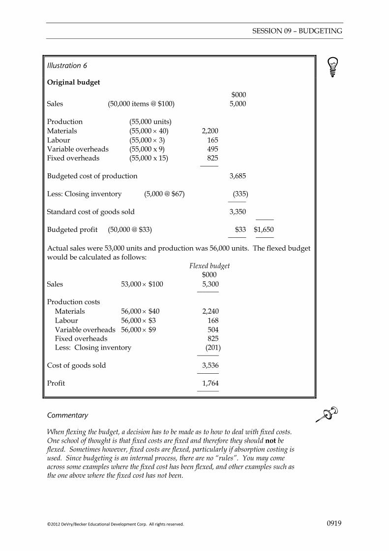
SESSION 09 – BUDGETING
©2012 DeVry/Becker Educational Development Corp. All rights reserved. 0919
Illustration 6
Original budget
$000 Sales (50,000 items @ $100) 5,000 Production (55,000 units) Materials (55,000 × 40) 2,200 Labour (55,000 × 3) 165 Variable overheads (55,000 x 9) 495 Fixed overheads (55,000 x 15) 825 _____ Budgeted cost of production 3,685 Less: Closing inventory (5,000 @ $67) (335) _____ Standard cost of goods sold 3,350 _____ Budgeted profit (50,000 @ $33) $33 $1,650 _____ _____ Actual sales were 53,000 units and production was 56,000 units. The flexed budget would be calculated as follows: Flexed budget $000 Sales 53,000 × $100 5,300 ______ Production costs Materials 56,000 × $40 2,240 Labour 56,000 × $3 168 Variable overheads 56,000 × $9 504 Fixed overheads 825 Less: Closing inventory (201) ______ Cost of goods sold 3,536 ______ Profit 1,764 ______
Commentary When flexing the budget, a decision has to be made as to how to deal with fixed costs. One school of thought is that fixed costs are fixed and therefore they should not be flexed. Sometimes however, fixed costs are flexed, particularly if absorption costing is used. Since budgeting is an internal process, there are no “rules”. You may come across some examples where the fixed cost has been flexed, and other examples such as the one above where the fixed cost has not been.
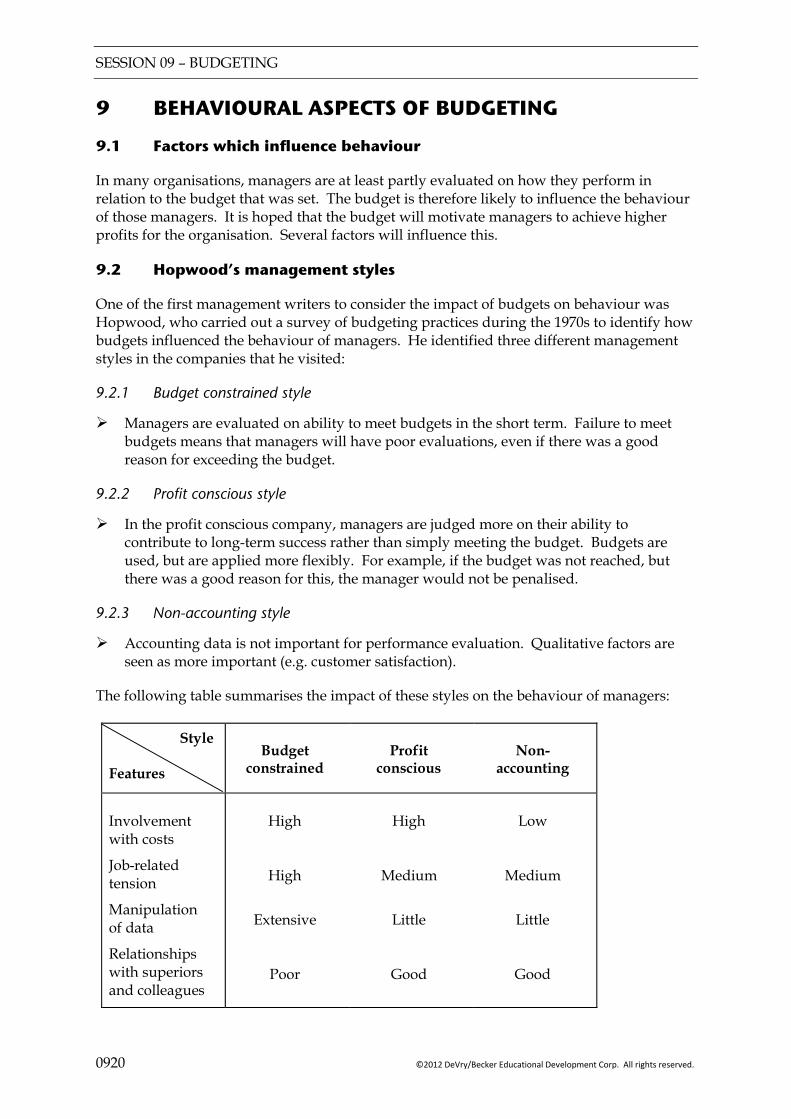
SESSION 09 – BUDGETING
0920 ©2012 DeVry/Becker Educational Development Corp. All rights reserved.
9 BEHAVIOURAL ASPECTS OF BUDGETING
9.1 Factors which influence behaviour
In many organisations, managers are at least partly evaluated on how they perform in relation to the budget that was set. The budget is therefore likely to influence the behaviour of those managers. It is hoped that the budget will motivate managers to achieve higher profits for the organisation. Several factors will influence this.
9.2 Hopwood’s management styles
One of the first management writers to consider the impact of budgets on behaviour was Hopwood, who carried out a survey of budgeting practices during the 1970s to identify how budgets influenced the behaviour of managers. He identified three different management styles in the companies that he visited:
9.2.1 Budget constrained style
Managers are evaluated on ability to meet budgets in the short term. Failure to meet budgets means that managers will have poor evaluations, even if there was a good reason for exceeding the budget.
9.2.2 Profit conscious style
In the profit conscious company, managers are judged more on their ability to contribute to long-term success rather than simply meeting the budget. Budgets are used, but are applied more flexibly. For example, if the budget was not reached, but there was a good reason for this, the manager would not be penalised.
9.2.3 Non-accounting style
Accounting data is not important for performance evaluation. Qualitative factors are seen as more important (e.g. customer satisfaction).
The following table summarises the impact of these styles on the behaviour of managers:
Style Features
Budget
constrained
Profit
conscious
Non-
accounting
Involvement with costs
Job-related tension
Manipulation of data
Relationships with superiors and colleagues
High
High
Extensive
Poor
High
Medium
Little
Good
Low
Medium
Little
Good
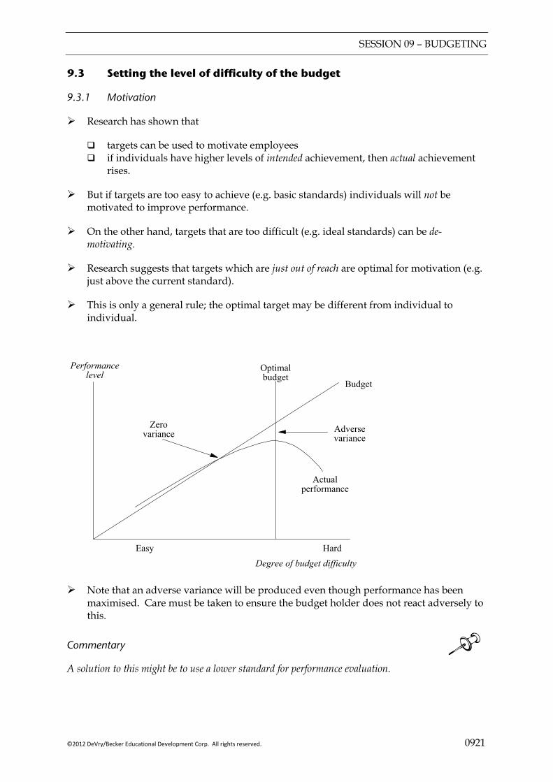
SESSION 09 – BUDGETING
©2012 DeVry/Becker Educational Development Corp. All rights reserved. 0921
9.3 Setting the level of difficulty of the budget
9.3.1 Motivation
Research has shown that
targets can be used to motivate employees if individuals have higher levels of intended achievement, then actual achievement
rises.
But if targets are too easy to achieve (e.g. basic standards) individuals will not be motivated to improve performance.
On the other hand, targets that are too difficult (e.g. ideal standards) can be de-motivating.
Research suggests that targets which are just out of reach are optimal for motivation (e.g. just above the current standard).
This is only a general rule; the optimal target may be different from individual to individual.
Optimalbudget
Zerovariance
Actualperformance
Adversevariance
Budget
Easy HardDegree of budget difficulty
Performancelevel
Note that an adverse variance will be produced even though performance has been maximised. Care must be taken to ensure the budget holder does not react adversely to this.
Commentary A solution to this might be to use a lower standard for performance evaluation.
SESSION 09 – BUDGETING
0922 ©2012 DeVry/Becker Educational Development Corp. All rights reserved.
9.4 Standards
When sitting the level of budget difficulty, three approaches can be used to setting standards:
9.4.1 Ideal standard
Calculated assuming 100% efficiency from all factors of production (e.g. no losses, no idle time, etc).
Too difficult as a target, therefore may lead to de-motivation.
9.4.2 Basic standard
Long-run (underlying) average standard. Based on historic data (i.e. past performance). Out of date. Likely to be too easy to achieve in the future.
9.4.3 Expected standard
Based on normal efficiency (e.g. after normal loss, expected idle time, normal machine down time).
May be a useful standard to use in variance analysis.
But may not be an appropriate target for motivation as can be met without any improvement over normal efficiency.
9.4.4 Current standard
A standard established for use over a short period of time, reflecting current conditions.
Obtained by adjusting the expected standard.
Use is time consuming (e.g. new current standards must be recalculated each month).
9.5 Benefits and difficulties of employee participation
The benefits of bottom-up budgeting, whereby managers or employees participate in the setting of their budgets, have already been discussed earlier in this session. The same benefits apply to setting other performance targets.
9.5.1 Benefits of employee participation
Employees are more likely to accept and work towards targets they have been involved in setting.
Employees will be more motivated if they are given more autonomy
The targets should be realistic, as employees would not agree to targets that are not.

SESSION 09 – BUDGETING
©2012 DeVry/Becker Educational Development Corp. All rights reserved. 0923
9.5.2 Potential problems of employee participation
Employees may try to set targets that are too easy. In budgets, they may add “slack” to the budgets. Budgetary slack means adding expenses to the budget in excess of what is really needed.
Setting the targets is likely to be more time consuming if employees are involved.
Setting of targets may not be fair, given that some employees will be better negotiators than others and will therefore be able to negotiate lower targets.
Key points
A budgetary control system is a means of management exercising control over the organisation by setting budgets, and comparing the performance of the organisation against the budget. Action is taken to remedy deviations from the budget.
The main objectives of budgetary control system are planning, coordination of the activities of the organisation and ensuring better resource utilisation. Budgets may also be used to delegate responsibility to managers, who are then evaluated on how they perform relative to the budget.
Budgets should contribute towards the long-term plans of the organisation.
Top-down budgeting means that budgets are prepared by senior management and imposed on the departments responsible for achieving them. Bottom-up budgeting means that departments participate in preparing their own budgets.
Incremental budgeting is where the starting point for the preparation of a budget is the previous year’s budget or actual figures. ZBB is where the preparation of the budget starts from zero and the costs and benefits of all activities have to be quantified and justified.
Budgets influence the behaviour of managers, since their evaluation depends on whether they achieve the budget.
The difficulty of a budget should be sufficient to challenge, but not unachievable, or it will demotivate.
SESSION 09 – BUDGETING
0924 ©2012 DeVry/Becker Educational Development Corp. All rights reserved.
FOCUS
You should now be able to:
outline the objectives of a budgetary control system;
explain how corporate and divisional objectives may differ and can be reconciled;
identify and resolve conflicting objectives and explain implications;
explain how budgets fit in with the performance hierarchy;
select and explain appropriate budgetary systems for an organisation, including top-down, bottom-up, rolling, zero-base, activity-based, incremental and feed-forward control;
describe the information used in budget systems and the sources of the information needed;
explain the difficulties of changing a budget system;
explain how budget systems can deal with uncertainty in the environment;
indicate the usefulness and problems with different budget types (zero-based, activity-based, incremental, master, functional and flexible;
explain the difficulties of changing a budgetary system;
identify the factors which influence behaviour;
discuss the issues surrounding setting the difficulty level for a budget;
explain the benefits and difficulties of the participation of employees in the negotiation of targets.
SESSION 09 – BUDGETING
©2012 DeVry/Becker Educational Development Corp. All rights reserved. 0925
EXAMPLE SOLUTIONS
Solution 1
Advantages of top-down budgeting
Senior management have greater control of the budgetary process. The budgets will therefore reflect more accurately the corporate objectives and the long-term plan.
Where managers prepare their own budgets, and are assessed on how they perform relative to these, there is a temptation for the managers to add “budgetary slack” (i.e. they overstate budgeted expenses or understate budgeted revenues to make their budgets easier to achieve). Using top-down budgeting avoids this risk.
Since budgets are prepared centrally, the activities of the various departments should be better coordinated.
It may be difficult for managers with little financial or accounting knowledge to prepare budgets for their own departments. Top-down budgeting means that these managers would not have to prepare their own budgets.
The various budgets are more likely to be set at the same level of difficulty and would therefore be fairer than if bottom-up budgeting is used.
Advantages of bottom-up budgeting
Managers are more likely to accept the budgeted targets for their departments and work towards achieving them if they have been involved in setting the budgets.
Managers have a more detailed knowledge of the work that their departments do than senior management, and can therefore produce more realistic budgets.
Managers may feel more motivated if they are given greater autonomy and more responsibility for their departments. Giving managers greater autonomy would normally include giving them the right to participate in preparing their own budgets.
At the end of the budget period, when managers performance is being assessed, the managers cannot claim that they budget was unrealistic if they prepare the budget.
Managers will better understand the financial objectives of the organisation if they are involved in budgeting. Thus the budget process can be seen as a type of education given to non-financial managers.

SESSION 09 – BUDGETING
0926 ©2012 DeVry/Becker Educational Development Corp. All rights reserved.
Solution 2
Food retailer
Food retailing is a stable business. Few unexpected external changes are likely to occur. Therefore little benefit would be gained by continuously updating budgets, so rolling budgets are unlikely to be used.
Manufacturer of mobile computer devices and mobile telephones
This industry is very dynamic as new products are constantly being developed. As competitors introduce new products, this may well change demand for the companies own products. It may also impact on whether or not existing development projects are speeded up, scrapped or changes. Accordingly, rolling budgets may be useful in this type of business.
Airlines
Airlines are also subject to many external factors. Fuel typically accounts for 50% of the total costs of many airlines, so changes in the market price of oil will impact on profits. Economic factors impact heavily on demand, since travel is a “discretionary” activity for many travellers. Accordingly rolling budgets may be useful, as otherwise budgets could become out of date very quickly.
Advertising agencies
Budgeting is likely to be very difficult in advertising agencies. Revenues may vary significantly from month to month depending on whether or not clients decide to spend on campaigns. Accordingly rolling forecasts could be useful.
Retail banking
Retail banking is a fairly stable business. As such, little benefit may be gained from using rolling budgets.
Solution 3
In practice most governments use incremental budgeting. Due to the sheer size of central government budgets, introducing zero-based budgeting would be very time consuming.
There are however very good arguments in favour of using ZBB in central governments. Much government spending is discretionary in nature. ZBB would enable governments to re-examine the benefits associated with this discretionary expenditure and decide whether or not to continue to allocate so much of the state’s funds to these types of activities.
In recent years, many governments in the European Union appear to have lost control of their spending and are having to make cut backs to correct high budget deficits. Countries such as Greece, Spain and the UK are now looking for ways to reduce spending. ZBB could be a very useful tool in this.

SESSION 09 – BUDGETING
©2012 DeVry/Becker Educational Development Corp. All rights reserved. 0927
Certain areas of government expenditure may not be discretionary (e.g. spending in areas of welfare benefits and health services may be determined by demand for those services). As such, ZBB would not be appropriate. In other areas (e.g. funding for arts and culture and defence) ZBB could be useful as these are areas where governments have discretion as to how much to spend.
Due to the huge amount of work involved in ZBB it is unlikely that it would be carried out annually. However, it could be performed over a longer period (e.g. every five years) with incremental budgeting used during the interim periods.
Solution 4 — Activity Based Budgeting
Advantages of ABB
Management attention is focussed on the activities of the organisation. These are something that management can control more easily than focussing on total costs.
Better understanding of what causes costs to be incurred may provide opportunities for cost reductions.
May identify non-value added activities which can be estimated.
Disadvantages of ABB
Complicated and expensive to implement. More suited to large organisations with multiple products and many drivers.
Many fixed costs do not vary with changes in the volume of drivers in the short run – so ABB may provide misleading information.

SESSION 09 – BUDGETING
0928 ©2012 DeVry/Becker Educational Development Corp. All rights reserved.
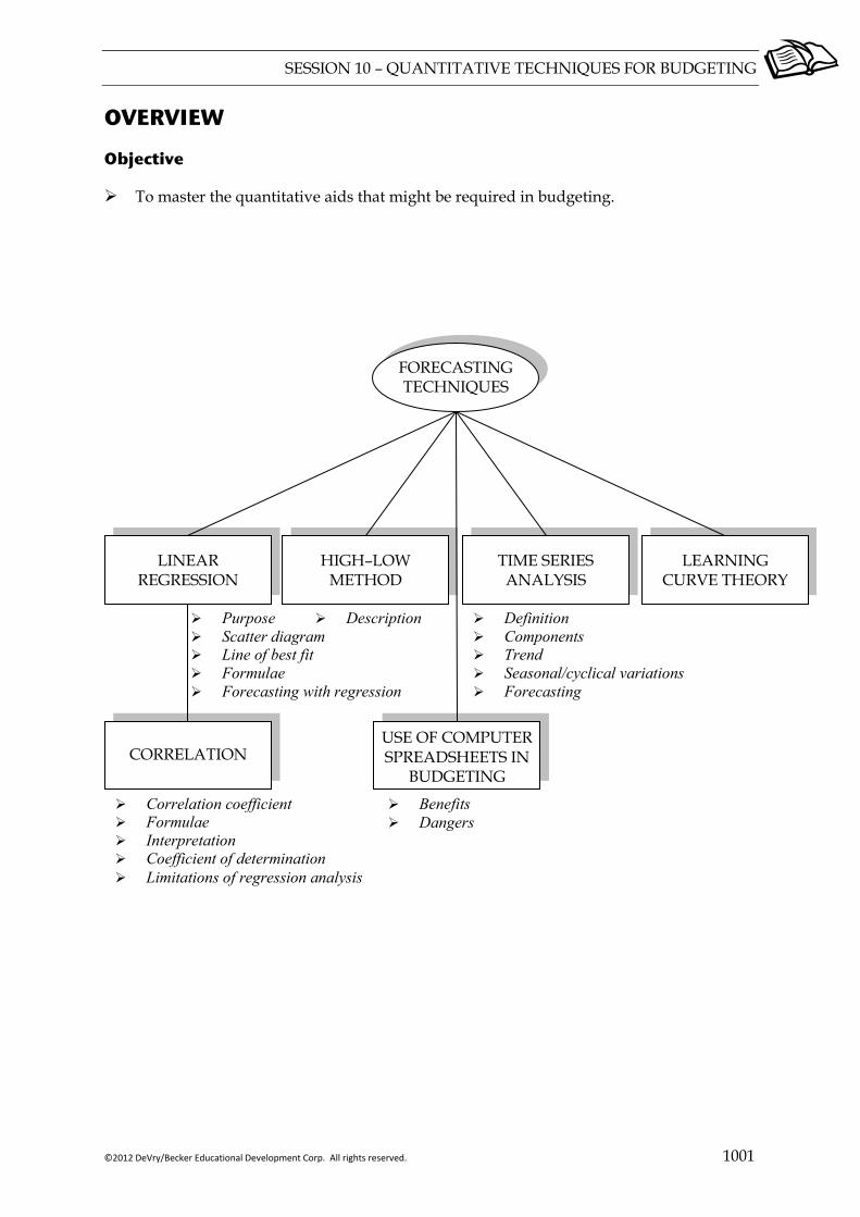
SESSION 10 – QUANTITATIVE TECHNIQUES FOR BUDGETING
©2012 DeVry/Becker Educational Development Corp. All rights reserved. 1001
OVERVIEW
Objective
To master the quantitative aids that might be required in budgeting.
LINEAR REGRESSION
LEARNING CURVE THEORY
TIME SERIES ANALYSIS
Purpose Scatter diagram Line of best fit Formulae Forecasting with regression
HIGH–LOW METHOD
Definition Components Trend Seasonal/cyclical variations Forecasting
FORECASTING TECHNIQUES
CORRELATION
Correlation coefficient Formulae Interpretation Coefficient of determination Limitations of regression analysis
USE OF COMPUTER SPREADSHEETS IN
BUDGETING
Benefits Dangers
Description

SESSION 10 – QUANTITATIVE TECHNIQUES FOR BUDGETING
1002 ©2012 DeVry/Becker Educational Development Corp. All rights reserved.
1 LINEAR REGRESSION AND CORRELATION
1.1 Purpose
There are various techniques which can be used to try to predict future costs from historical data.
The aim is to try to predict levels of costs at different output levels to assist in decision making and planning
1.2 Scatter diagram
In practice there is often a causal relationship between the two variables in question. For example:
Costs depend on volume not vice versa
Dependent variable
Independent variable
Usually the independent variable is denoted by x and plotted horizontally, whilst the dependent variable is denoted by y and plotted vertically.
Normally the first step is to plot the collected data on a scatter diagram. If the variables are related, a pattern will emerge.
x x
x x
x x x
x x
x x
x x
x x x
x x x
x x x
x x x x x x
x x x x
x
x x
x x x x
x x
x x
x x x x
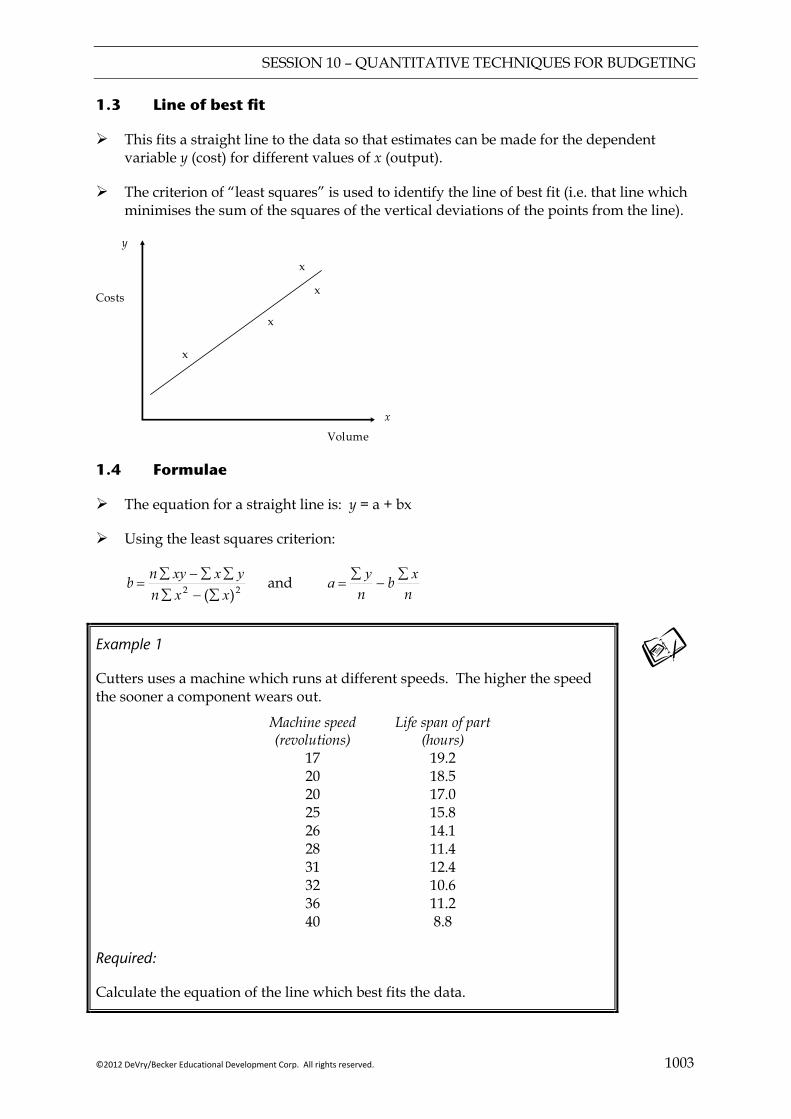
SESSION 10 – QUANTITATIVE TECHNIQUES FOR BUDGETING
©2012 DeVry/Becker Educational Development Corp. All rights reserved. 1003
1.3 Line of best fit
This fits a straight line to the data so that estimates can be made for the dependent variable y (cost) for different values of x (output).
The criterion of “least squares” is used to identify the line of best fit (i.e. that line which minimises the sum of the squares of the vertical deviations of the points from the line).
Costs
x
x
x
x
x
y
Volume
1.4 Formulae
The equation for a straight line is: y = a + bx
Using the least squares criterion:
22 )( xxyxxy
∑−∑∑∑−∑
=nnb and
nb
nxya ∑
−∑
=
Example 1
Cutters uses a machine which runs at different speeds. The higher the speed the sooner a component wears out.
Machine speed Life span of part (revolutions) (hours) 17 19.2 20 18.5 20 17.0 25 15.8 26 14.1 28 11.4 31 12.4 32 10.6 36 11.2 40 8.8 Required:
Calculate the equation of the line which best fits the data.

SESSION 10 – QUANTITATIVE TECHNIQUES FOR BUDGETING
1004 ©2012 DeVry/Becker Educational Development Corp. All rights reserved.
Solution
x y xy x2 y2
17
20
20
25
26
28
31
32
36
40
19.2
18.5
17.0
15.8
14.1
11.4
12.4
10.6
11.2
8.8
_______ _______
_______ _______
_______ _______
_______ _______
_______ _______
Now substitute into the formulae (start with b)
n =
b
=
a
=
y =
1.5 Forecasting with regression
This data can now be substituted into the straight line formula and values of y can be predicted for chosen values of x.
Illustration 1
For example if a machine operates at 30 revolutions per minute, then by setting x equal to 30
y = 26.55 − 0.46 × 30 = 12.75
SESSION 10 – QUANTITATIVE TECHNIQUES FOR BUDGETING
©2012 DeVry/Becker Educational Development Corp. All rights reserved. 1005
2 CORRELATION
2.1 Correlation coefficient (r)
The reliability of predictions depends upon how closely the line fits the data
If the data fits the line perfectly it is said to be perfectly correlated
If the scatter diagram reveals no pattern at all, the variables are said to be uncorrelated
2.2 Formulae
The degree of correlation (r) is calculated as follows:
])(][)([ 2222 yyxxyxxy
∑−∑∑−∑
∑∑−∑=
nnnr
When r = +1 there is perfect positive linear correlation (i.e. all points lie on a straight line with a positive gradient).
When r = –1 there is perfect negative linear correlation (i.e. all points lie on a straight line with a negative gradient).
As r tends to 0 the less close is the linear relationship.
2.3 Interpretation of r — cause and effect
A high correlation between two variables does not necessarily justify the conclusion that a causal relationship exists
There may be no direct connection at all, in which case the correlation is termed spurious correlation.
This can occur for two reasons:
There may be an indirect connection whereby both x and y depend on a third variable;
The correlation may be due entirely to chance.
Example 2
Using Example 1, calculate the correlation coefficient.
Solution

SESSION 10 – QUANTITATIVE TECHNIQUES FOR BUDGETING
1006 ©2012 DeVry/Becker Educational Development Corp. All rights reserved.
2.4 Coefficient of determination (r2)
The purpose of this is to measure the extent to which the total variations in the dependent variable are due to the relationship between the two variables
It indicates the proportion of the variance of the dependent variable from its mean value which is explained by the independent variable.
It is a measure of the cause of the variation – unlike the correlation coefficient.
2.5 Limitations of regression analysis
Number of variables – a number of other variables may also be relevant.
Linearity – the relationship between variables may not be linear.
Dangers in extrapolation – using regression analysis to estimate costs for a level of activity outside the range currently known is dangerous.
Amount of data – this may be limited.
Accuracy of data – the data may not be accurate.
Significance of correlation coefficient – this may be less than perfect.
Interpretation of relationship – the relationship may have arisen for spurious reasons.
3 HIGH—LOW METHOD
3.1 Description
A crude method of estimating a value of y (cost) for a value of x (volume)
It selects costs associated with the highest and lowest levels of activity (i.e. x) and assumes all other costs lie on a straight line
This method is limited by its crudeness. Furthermore, the use of extreme values to determine the relationship between two variables is probably dangerous, as extreme values are likely to be atypical.
Example 3
Output Costs $ 3,000 3,500 2,400 3,000 3,600 4,350 4,000 4,800
Required:
Find the equation y = a + bx. Where y is cost and x is output level.

SESSION 10 – QUANTITATIVE TECHNIQUES FOR BUDGETING
©2012 DeVry/Becker Educational Development Corp. All rights reserved. 1007
Solution
High
Low
y = a + bx
Gradient, b =
Substituting in
when x = y =
a =
y = 4 FORECASTING TECHNIQUES
4.1 Need for forecasting
Management accountants need to use forecasts for many areas of their work. In budgeting, for example, it is useful to be able to forecast sales. This session looks at some mathematical forecasting techniques.
4.2 Simple average growth models
Such models take average growth from the past, using the geometric mean, and assume that this level of growth will continue in the future.
SESSION 10 – QUANTITATIVE TECHNIQUES FOR BUDGETING
1008 ©2012 DeVry/Becker Educational Development Corp. All rights reserved.
Illustration 2
The sales of Beta during the last three years were as follows:
Year Sales $000 2008 100 2009 180 2010 210 2011 300 The growth rate of sales each year is as follows:
2009 80% (180 -100)/100 2010 16.67% (210 -180)/180 2011 42.9% (300-210)/210 The simple average growth rate is 46.5% (80% + 16.67% + 42.9%)/ 3. This overstates the rate of growth however; if the 2008 sales of $100,000 were to increase by 46.5% each year for three years, the sales in 2011 would be $314,000 not $300,000. The more accurate growth rate is obtained using the geometric mean. Growing by 80% is the same as multiplying by 1.8 , so the geometric mean for the three years is 3 429.11667.18.1 ×× = 1.442, so the average growth rate is 44.2%. This can then be used to calculate expected sales in future period.
4.3 Time series analysis (trend analysis)
A more sophisticated method of forecasting is known as time series analysis. This technique takes account of past growth rates, but also takes into account seasonal variations that may occur. Seasonal variations occur in many businesses- in retail, for example, sales are often high in the final quarter of the year, as people buy presents for the Christmas period, and sales fall significantly in the first quarter of the year.
Definition
A set of figures relating to the changing values of a variable over a period of time (e.g. quarterly sales).

SESSION 10 – QUANTITATIVE TECHNIQUES FOR BUDGETING
©2012 DeVry/Becker Educational Development Corp. All rights reserved. 1009
4.4 Components of a time series
A time series is a set of data recorded over a period of time. It could be made up of:
Trend (T) The “long-term” effect when fluctuations have been smoothed out
Cyclical variation (C) A cyclical fluctuation over a number of years (e.g. a five-yearly cycle of booms and depressions).
Seasonal variation (S) An annual cycle of variations due to seasonal influences.
Residual variations (R) Randomly occurring variations due to non-recurring influences.
4.5 Calculation of the trend
4.5.1 Methods
Linear regression − only suitable if trend is linear. It spans all the data.
Moving average − an average over complete cycles, moving along one period at a time. Some data at each end is lost in the averaging. For an even number of periods per cycle (e.g. a 4 quarterly cycle), the moving average must be centred by averaging in pairs.
4.5.2 Moving average
Calculate a moving total for whatever number of periods makes up a normal cycle (usually a year).
Calculate a moving average by dividing the moving total by the number of periods in a normal cycle. This is the trend figure (T).
(As a trend figure is required for each specific period, where the moving average is made up of an even number of periods, the trend figure must finally be found by averaging two of the moving average figures.)

SESSION 10 – QUANTITATIVE TECHNIQUES FOR BUDGETING
1010 ©2012 DeVry/Becker Educational Development Corp. All rights reserved.
Illustration 3
Quarter Sales 4 quarter 4 quarter Average moving moving total average $000 $000 $000 $000 2009 1 116 2 160 636 159 3 140 162 660 165 4 220 165 660 165 2010 1 140 2 160
162 is the trend figure for 2009 quarter 3 165 is the trend figure for 2009 quarter 4
If the trend is linear, then linear regression may be used.
4.6 Calculation of seasonal or cyclical variations
4.6.1 Additive model
For each trend value (T), calculate A − T where A is the actual data
Average all the values for the same period in a cycle (e.g. all the figures relating to quarter 1) so that one average is obtained for each of the periods in the normal cycle.
Quarterly data will have four averages, one for each quarter.
Apply a suitable adjustment to make the total of the averages equal zero The resulting values are the seasonal (S) or cyclical (C) values.

SESSION 10 – QUANTITATIVE TECHNIQUES FOR BUDGETING
©2012 DeVry/Becker Educational Development Corp. All rights reserved. 1011
Illustration 3 — continued
Quarter Trend Actual (T) (A) (A – T) 2010 3 162 140 – 22 4 165 220 55 2011 1 167 140 – 27 2 171 160 – 11 3 176 156 – 20 4 179 236 57 Quarters 1 2 3 4 2010 – 22 55 2011 – 27 –11 – 20 57 ___ ___ ___ ___ – 27 – 11 – 42 112 Average – 27 – 11 – 21 56
Total of averages: Adjustments Final variations Quarter 1 – 27 + 1 – 26 2 – 11 – 11 3 – 21 + 1 – 20 4 56 + 1 57 ___ ___ – 3 0 ___ ___
4.6.2 Multiplicative model (proportional method)
Using the multiplicative model A is expressed as a % of T to give a seasonal index.
The seasonal figures are then tabulated to calculate the average seasonal indices for each quarter.
SESSION 10 – QUANTITATIVE TECHNIQUES FOR BUDGETING
1012 ©2012 DeVry/Becker Educational Development Corp. All rights reserved.
Illustration 4 — Using the data from illustration 3
Quarter Trend Actual (T) (A) A/T x 100 2010 3 162 140 86.4% 4 165 220 133.3% 2011 1 167 140 83.8% 2 171 160 93.6% 3 176 156 88.6% 4 179 236 131.8% Quarters 1 2 3 4 2010 86.4 133.3 2011 83.8 93.6 88.6 131.8 _____ _____ _____ _____ Total 83.8 93.6 175 265.1 _____ _____ _____ _____ Average 83.8 93.6 87.5 132.6
Example 4
Given below are the quarterly sales figures for a new business for the first four years of trade.
Quarter 2008 2009 2010 2011 $000 $000 $000 $000 1 400 410 430 500 2 320 320 330 350 3 80 90 100 100 4 180 200 200 220
Required:
Analyse this data using time series analysis.
SESSION 10 – QUANTITATIVE TECHNIQUES FOR BUDGETING
©2012 DeVry/Becker Educational Development Corp. All rights reserved. 1013
Solution
Use moving total and average to calculate trend: Quarter 4 period
moving total 4 period
moving average Trend
(T) (A-T)
$000 $000 $000 $000 $000 2008 1 400 2 320 3 80 4 180 2009 1 410 2 320 3 90 4 200 2010 1 430 2 330 3 100 4 200 2011 1 500 2 350 3 100 4 220 Average the seasonal factors:
Quarter 1 2 3 4 2008 2009 2010 2011
Average
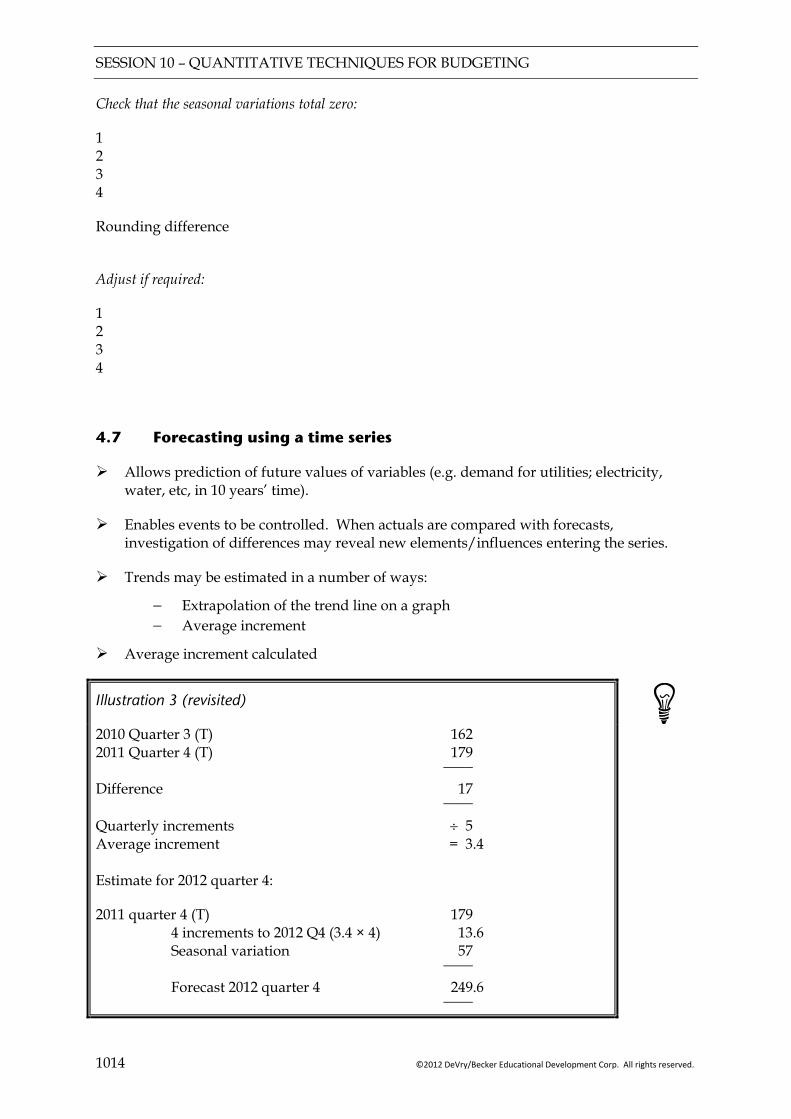
SESSION 10 – QUANTITATIVE TECHNIQUES FOR BUDGETING
1014 ©2012 DeVry/Becker Educational Development Corp. All rights reserved.
Check that the seasonal variations total zero:
1 2 3 4
Rounding difference
Adjust if required:
1 2 3 4
4.7 Forecasting using a time series
Allows prediction of future values of variables (e.g. demand for utilities; electricity, water, etc, in 10 years’ time).
Enables events to be controlled. When actuals are compared with forecasts, investigation of differences may reveal new elements/influences entering the series.
Trends may be estimated in a number of ways:
− Extrapolation of the trend line on a graph − Average increment
Average increment calculated
Illustration 3 (revisited)
2010 Quarter 3 (T) 162 2011 Quarter 4 (T) 179 ____
Difference 17 ____
Quarterly increments ÷ 5 Average increment = 3.4 Estimate for 2012 quarter 4:
2011 quarter 4 (T) 179 4 increments to 2012 Q4 (3.4 × 4) 13.6 Seasonal variation 57 ____
Forecast 2012 quarter 4 249.6 ____
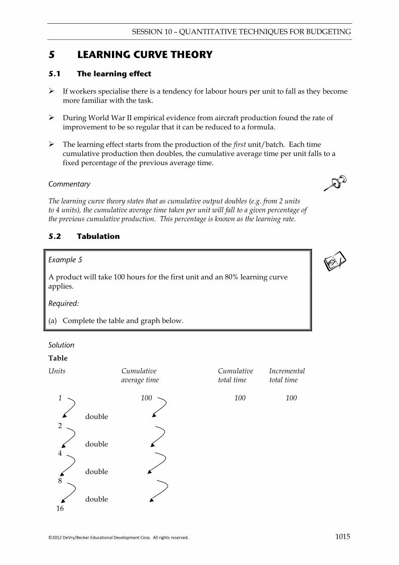
SESSION 10 – QUANTITATIVE TECHNIQUES FOR BUDGETING
©2012 DeVry/Becker Educational Development Corp. All rights reserved. 1015
5 LEARNING CURVE THEORY
5.1 The learning effect
If workers specialise there is a tendency for labour hours per unit to fall as they become more familiar with the task.
During World War II empirical evidence from aircraft production found the rate of improvement to be so regular that it can be reduced to a formula.
The learning effect starts from the production of the first unit/batch. Each time cumulative production then doubles, the cumulative average time per unit falls to a fixed percentage of the previous average time.
Commentary The learning curve theory states that as cumulative output doubles (e.g. from 2 units to 4 units), the cumulative average time taken per unit will fall to a given percentage of the previous cumulative production. This percentage is known as the learning rate.
5.2 Tabulation
Example 5
A product will take 100 hours for the first unit and an 80% learning curve applies.
Required:
(a) Complete the table and graph below.
Solution
Table
Units Cumulative Cumulative Incremental average time total time total time
1 100 100 100 double
2 double
4 double
8 double
16
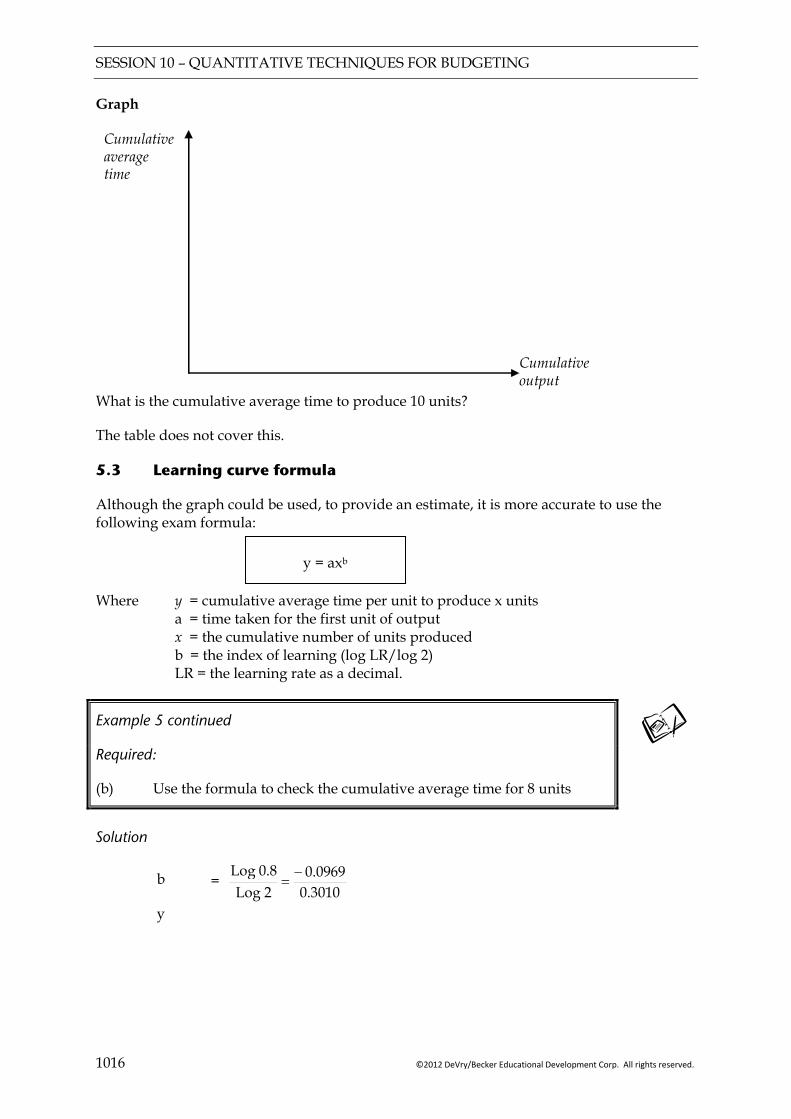
SESSION 10 – QUANTITATIVE TECHNIQUES FOR BUDGETING
1016 ©2012 DeVry/Becker Educational Development Corp. All rights reserved.
Graph
Cumulative average time
Cumulative output
What is the cumulative average time to produce 10 units?
The table does not cover this.
5.3 Learning curve formula
Although the graph could be used, to provide an estimate, it is more accurate to use the following exam formula:
y = axb
Where y = cumulative average time per unit to produce x units a = time taken for the first unit of output x = the cumulative number of units produced b = the index of learning (log LR/log 2) LR = the learning rate as a decimal.
Example 5 continued
Required:
(b) Use the formula to check the cumulative average time for 8 units
Solution
b = 0.30100.0969
2Log 0.8Log −
=
y
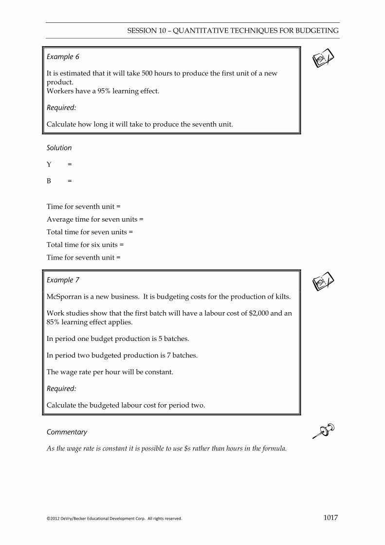
SESSION 10 – QUANTITATIVE TECHNIQUES FOR BUDGETING
©2012 DeVry/Becker Educational Development Corp. All rights reserved. 1017
Example 6
It is estimated that it will take 500 hours to produce the first unit of a new product. Workers have a 95% learning effect.
Required:
Calculate how long it will take to produce the seventh unit.
Solution
Y =
B =
Time for seventh unit =
Average time for seven units =
Total time for seven units =
Total time for six units =
Time for seventh unit =
Example 7
McSporran is a new business. It is budgeting costs for the production of kilts.
Work studies show that the first batch will have a labour cost of $2,000 and an 85% learning effect applies.
In period one budget production is 5 batches.
In period two budgeted production is 7 batches.
The wage rate per hour will be constant.
Required:
Calculate the budgeted labour cost for period two.
Commentary As the wage rate is constant it is possible to use $s rather than hours in the formula.
SESSION 10 – QUANTITATIVE TECHNIQUES FOR BUDGETING
1018 ©2012 DeVry/Becker Educational Development Corp. All rights reserved.
Labour cost for period two =
b = 2Log
0.85Log 3010.00706.0−
Total cost for 12 batches =
Total cost for 5 batches =
Labour cost for period two =
In practice (and in many questions) the learning curve effect does not continue forever. At some point a “steady state” is reached – beyond this point hours per unit is constant.
5.4 Conditions for a learning curve to apply
The activity is labour intensive. The units are identical (i.e. a repetitive task). Low labour turnover. No prolonged breaks in production.
Commentary Unfortunately such conditions may lead to low morale and hence reduce the learning effect.
5.5 Applications of learning curve theory
Standard setting – the labour standard should be set/revised based upon the expected learning effect.
Budgeting – variable costs are expected to fall with an increase in production – particularly important to cash budgeting.
Pricing decisions – an accurate labour cost may be predicted into the future.
Work scheduling – manpower planning (e.g. as part of MRPII).
Commentary MRPII is a manufacturing resource planning system which integrates functions in a manufacturing firm. It encompasses production scheduling, job costing, control of workforce, performance measurement, etc.

SESSION 10 – QUANTITATIVE TECHNIQUES FOR BUDGETING
©2012 DeVry/Becker Educational Development Corp. All rights reserved. 1019
5.6 Reservations with the learning curve
When using the learning curve in practice, there are some weaknesses:
Knowing what the learning rate will be for new products. The usual assumption is that it will be similar to products made in the past. This may not always be a valid assumption.
The learning curve is useful in situations where production of a product takes place on a continuous basis. If there is a break in production, however, workers may “forget” the skill and the learning curve will not be so predictable.
In the modern business world, many products are tailor made for customers- the idea of mass producing identical items, which is where learning curves are strongest, is not always appropriate.
In some heavily unionised industries there may be “go slow” agreements where workers agree not to work to their full capacity in order to save jobs.
6 USE OF COMPUTER SPREADSHEETS IN BUDGETING
The use of spreadsheet applications such as Microsoft Excel or Lotus 123 is widespread in most organisations, and budgeting is one area where spreadsheets are likely to be use. Advantages of using spreadsheets in budgeting are:
6.1 Benefits of using spreadsheets in budgeting
Budgets may contain many lines of detail. By preparing budgets in spreadsheets, any line of the budget can easily be changed, and it is not necessary to manually add up the budget totals.
Flexed budgets can easily be performed using spreadsheets. All the user would need to do is to change the value in the sales units’ cell, and all the other cells would automatically be recalculated.
Master budgets, which are summarised budgets for the whole organisation can be prepared in the same spreadsheet and linked into the subsidiary budgets, so that any changes to the subsidiary budgets will automatically be reflected in the master budget.
6.2 Dangers of using spreadsheets in budgeting
It is easy for errors to appear in formulas in spreadsheet models. This may mean that budgeted figures may be incorrect if they are based on an incorrect formula.
Because users may be familiar with spreadsheet models, they may change parts of the standard budgeting proformas without authorisation.

SESSION 10 – QUANTITATIVE TECHNIQUES FOR BUDGETING
1020 ©2012 DeVry/Becker Educational Development Corp. All rights reserved.
Key points
Linear regression is used to identify the relationship between two variables based on sample data.
The correlation coefficient measures how well changes in the dependent variable can be explained by changes in the independent variable. It can take any value between 1 and -1.
The high low method is a crude method used to find the relationship, which takes only the highest and lowest values from the sample.
Trend analysis can also be used to determine the relationship between two variables, but is used more commonly to determine the change in the value of a variable over time.
FOCUS
You should now be able to:
analyse fixed and variable cost elements from total cost data using high/low and
regression analysis;
explain the use of forecasting techniques, including time series, simple average growth models and estimates based on judgement and experience. Predict a future value from provided time series analysis data using both additive and proportional data;
estimate the learning effect and apply the learning curve to a budgetary problem, including calculations on steady states;
discuss the reservations with the learning curve;
explain the benefits and dangers inherent in using spreadsheets in budgeting.

SESSION 10 – QUANTITATIVE TECHNIQUES FOR BUDGETING
©2012 DeVry/Becker Educational Development Corp. All rights reserved. 1021
EXAMPLE SOLUTIONS
Solution 1 — Line of best fit
x y xy x2 y2 17
20 20 25 26 28 31 32 36 40
19.2 18.5 17.0 15.8 14.1 11.4 12.4 10.6 11.2
8.8
326.4 370.0 340.0 395.0 366.6 319.2 384.4 339.2 403.2 352.0
289 400 400 625 676 784 961
1,024 1,296 1,600
368.65 342.25 289.00 249.64 198.81 129.96 153.76 112.36 125.44
77.44 _______
275 _______
_______ 139.0 _______
_______ 3,596.0 _______
_______ 8,055 _______
_______ 2,047.30 _______
n = 10 b
925,4265,2
)275(055,810139275596,310
2−
=−×
×−×= = – 0.4599
a 102754599.0
10139
×+= = 26.55
y = 26.55 – 0.46x Solution 2 — Correlation coefficient
=−×−×
×−×=
)1393.047,210)(275805510(
13927535961022
r11524925
265,2×
−= −0.9509
Solution 3 — High-low
High (4,000, 4,800) Low (2,400, 3,000)
y = a + bx
Gradient, b = 400,2 000,4000,3 800,4
−− =
600,1800,1 =
1618 = 1.125
Substituting in low level of activity (alternatively, use high level)
When x = 2,400 y = 3,000
3,000 = a + 1.125 × 2,400 3,000 = a + 2,700 a = 300
y = 300 + 1.125x
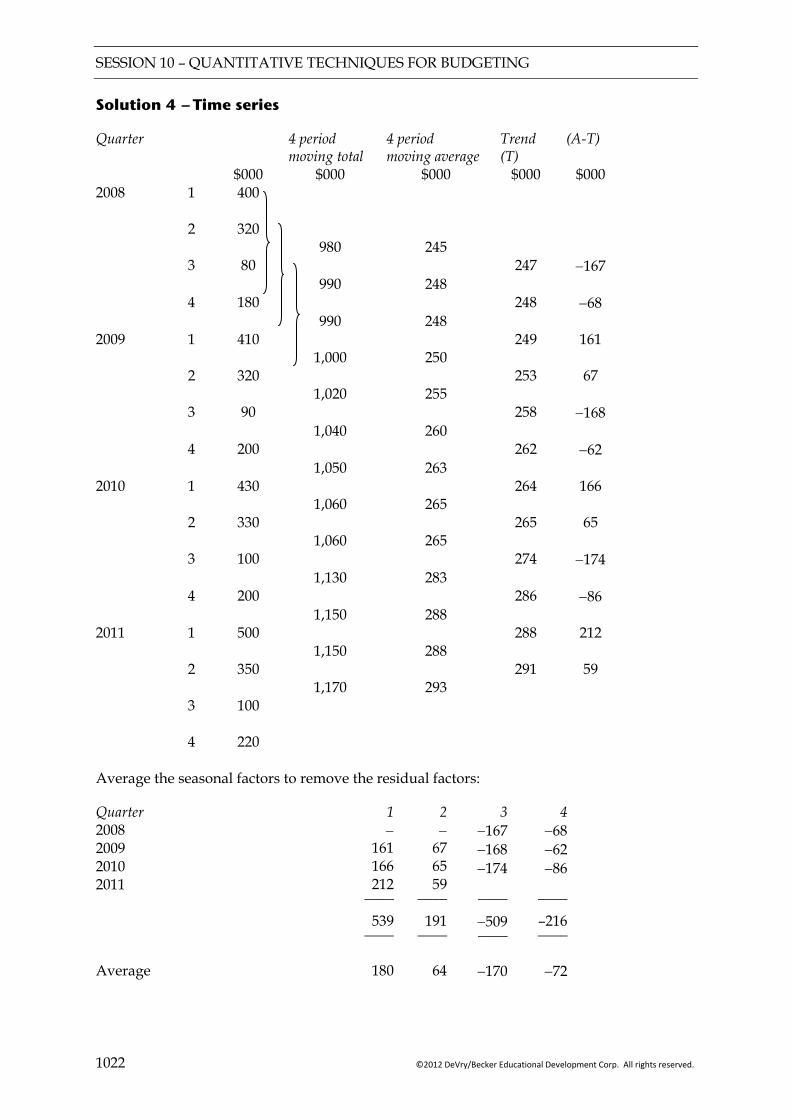
SESSION 10 – QUANTITATIVE TECHNIQUES FOR BUDGETING
1022 ©2012 DeVry/Becker Educational Development Corp. All rights reserved.
Solution 4 — Time series
Quarter 4 period moving total
4 period moving average
Trend (T)
(A-T)
$000 $000 $000 $000 $000 2008 1 400 2 320 980 245 3 80 247 −167 990 248 4 180 248 −68 990 248 2009 1 410 249 161 1,000 250 2 320 253 67 1,020 255 3 90 258 −168 1,040 260 4 200 262 −62 1,050 263 2010 1 430 264 166 1,060 265 2 330 265 65 1,060 265 3 100 274 −174 1,130 283 4 200 286 −86 1,150 288 2011 1 500 288 212 1,150 288 2 350 291 59 1,170 293 3 100 4 220 Average the seasonal factors to remove the residual factors:
Quarter 1 2 3 4 2008 2009 2010 2011
− 161 166 212
− 67 65 59
−167 −168 −174
−68 −62 −86
____ 539 ____
____ 191 ____
____ −509 ____
____ –216 ____
Average 180 64 −170 −72
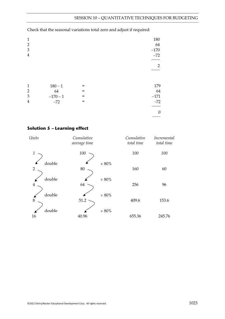
SESSION 10 – QUANTITATIVE TECHNIQUES FOR BUDGETING
©2012 DeVry/Becker Educational Development Corp. All rights reserved. 1023
Check that the seasonal variations total zero and adjust if required:
1 2 3 4
180 64
−170 −72
____
2 ____
1 2 3 4
180 − 1 64
−170 − 1 −72
= = = =
179 64
−171 −72
____
0 ____
Solution 5 — Learning effect
Units Cumulative Cumulative Incremental average time total time total time
1 100 100 100 double × 80%
2 80 160 60 double × 80%
4 64 256 96 double × 80%
8 51.2 409.6 153.6 double × 80%
16 40.96 655.36 245.76
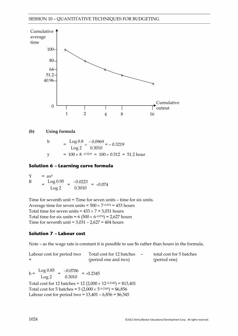
SESSION 10 – QUANTITATIVE TECHNIQUES FOR BUDGETING
1024 ©2012 DeVry/Becker Educational Development Corp. All rights reserved.
Cumulative average time
100
80
6451.2
40.96
0Cumulative output
x
x
x x
x
1 2 4 8 16
(b) Using formula
b = 0.30100.0969
2Log 0.8Log −
= = – 0.3219
y = 100 × 8 –0.3219 = 100 × 0.512 = 51.2 hour Solution 6 — Learning curve formula
Y = axb B =
2Log 0.95Log
= 3010.00223.0− = –0.074
Time for seventh unit = Time for seven units – time for six units. Average time for seven units = 500 × 7–0.074 = 433 hours Total time for seven units = 433 × 7 = 3,031 hours Total time for six units = 6 (500 × 6–0.074) = 2,627 hours Time for seventh unit = 3,031 – 2,627 = 404 hours Solution 7 — Labour cost
Note – as the wage rate is constant it is possible to use $s rather than hours in the formula.
Labour cost for period two =
Total cost for 12 batches (period one and two)
– total cost for 5 batches (period one)
b = 2Log
0.85Log =
3010.00706.0− = –0.2345
Total cost for 12 batches = 12 (2,000 × 12–0.2345) = $13,401 Total cost for 5 batches = 5 (2,000 × 5–0.2345) = $6,856 Labour cost for period two = 13,401 – 6,856 = $6,545
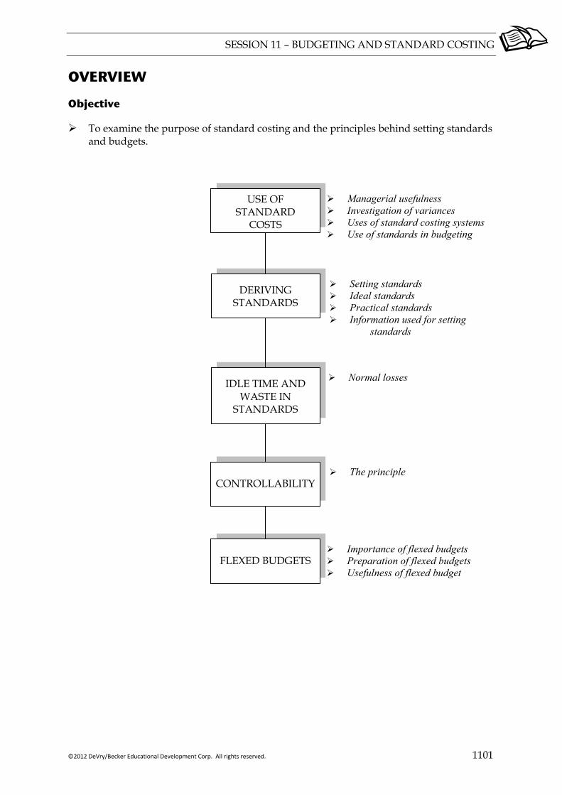
SESSION 11 – BUDGETING AND STANDARD COSTING
©2012 DeVry/Becker Educational Development Corp. All rights reserved. 1101
OVERVIEW
Objective
To examine the purpose of standard costing and the principles behind setting standards and budgets.
USE OF STANDARD
COSTS
Managerial usefulness Investigation of variances Uses of standard costing systems Use of standards in budgeting
Setting standards Ideal standards Practical standards Information used for setting
standards
The principle
DERIVING STANDARDS
IDLE TIME AND WASTE IN
STANDARDS
Normal losses
Importance of flexed budgets Preparation of flexed budgets Usefulness of flexed budget
CONTROLLABILITY
FLEXED BUDGETS

SESSION 11 – BUDGETING AND STANDARD COSTING
1102 ©2012 DeVry/Becker Educational Development Corp. All rights reserved.
1 USE OF STANDARD COSTS
1.1 Managerial usefulness
Production costs are affected by internal factors over which management has a large degree of control. An important role of executive management is to help departmental managers to understand their part in contributing to the success of the firm. Standard costs and the variances that arise from them:
keep management informed about the economy, efficiency and effectiveness of production processes;
facilitate supervisory personnel being made directly responsible for the variances under their control.
Variances provide a measure of the fairness of standards and facilitate further analysis, investigation, and action (e.g. to eliminate causes of undesirable variances). Adjustments should be made to unreasonable standard if variance analysis is to be meaningful. Variance analysis should encourage and reward cost control commensurate with desired levels of performance.
Definition
Standard cost: the predetermined cost of producing a single unit (or batch) of a product (goods or service) during a specific period in the near future. It is the planned cost of a product under current and/or anticipated operating conditions.
An example of a calculation of a standard cost, often referred to as a “standard cost card” is shown below:
Illustration 1 — Standard cost card (absorption costing)
Product XYZ $ per unitSales price 100 ___
Production Materials (2 kg @ $20/kg) 40 Labour (1½ hrs @ $2/hr) 3 Variable O/H (1½ hrs @ $6/hr) 9 Fixed O/H (1½ hrs @ $10/hr) 15 ___ Standard cost of production 67 ___ Standard profit per unit 33 ___
SESSION 11 – BUDGETING AND STANDARD COSTING
©2012 DeVry/Becker Educational Development Corp. All rights reserved. 1103
A standard provides a “benchmark” or “norm” for measuring performance. Standards are widely used (e.g. “RDA” (recommended daily allowances), drinking measures, materials standards for building constructions, quality standards, health and safety standards). In management accounting standards generally relate to two aspects of inputs used in producing goods/services:
Quantity standards specify how much resource (raw materials, labour) should be input to produce a unit of product/service.
Price (or cost) standards stipulate how much should be paid for each unit of resource.
The main reason for categorising standards – into price and quantity is because different managers are usually responsible for the activities of buying and using inputs which occur at different points in time. For example:
The purchasing manager’s responsibility is exercised when materials are purchased. The production or factory manager’s responsibility is exercised only when the materials are used, which could be months later (even in a different budget period). Differences between actual prices and standard prices and actual quantities and standard quantities are called variances. “Variance analysis” is the process of calculating and interpreting variances.
Management needs to investigate the significant variances revealed (by a comparison of actual quantities and prices against the standards) to establish their cause(s) and so take corrective action to prevent their reoccurrence. Management “By Exception” is facilitated because investigation is unnecessary if deviations are insignificant.
Commentary The notion of management by exception can be likened to switching on a desktop computer – press the button and it starts – there is no need to check that the power is on, cables connected, fan working, etc. The standard (expectation) is that the computer will start. Only if the expectation is not met is it necessary to investigate the discrepancy. An expectation that has not been met is an opportunity to uncover the root of the problem. If the underlying cause is not discovered and corrected, the problem is likely to recur and may worsen.
1.2 Investigation of variances
The main purpose of variance investigation is to improve operations. Actual cost and performance is compared with the standard cost of actual performance reports and the level of actual performance against what was expected (budgeted). The differences between actual results and what should have happened according to the standards are variances. Management should consider both their nature (“why did it arise?”) and magnitude (“why has it increased”?) A corrective action could include re-calibrating/re-setting the specifications of an item of equipment or changing a supplier. An amended standard cost may be prepared for the next period.
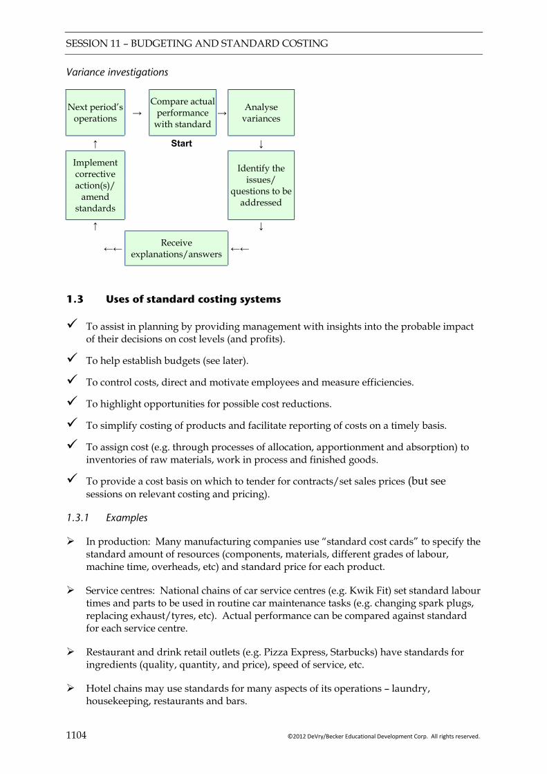
SESSION 11 – BUDGETING AND STANDARD COSTING
1104 ©2012 DeVry/Becker Educational Development Corp. All rights reserved.
Variance investigations
Next period’s operations →
Compare actual performance
with standard → Analyse
variances
↑ Start ↓
Implement corrective action(s)/
amend standards
Identify the issues/
questions to be addressed
↑ ↓
←← Receive explanations/answers ←←
1.3 Uses of standard costing systems
To assist in planning by providing management with insights into the probable impact of their decisions on cost levels (and profits).
To help establish budgets (see later).
To control costs, direct and motivate employees and measure efficiencies.
To highlight opportunities for possible cost reductions.
To simplify costing of products and facilitate reporting of costs on a timely basis.
To assign cost (e.g. through processes of allocation, apportionment and absorption) to inventories of raw materials, work in process and finished goods.
To provide a cost basis on which to tender for contracts/set sales prices (but see sessions on relevant costing and pricing).
1.3.1 Examples
In production: Many manufacturing companies use “standard cost cards” to specify the standard amount of resources (components, materials, different grades of labour, machine time, overheads, etc) and standard price for each product.
Service centres: National chains of car service centres (e.g. Kwik Fit) set standard labour times and parts to be used in routine car maintenance tasks (e.g. changing spark plugs, replacing exhaust/tyres, etc). Actual performance can be compared against standard for each service centre.
Restaurant and drink retail outlets (e.g. Pizza Express, Starbucks) have standards for ingredients (quality, quantity, and price), speed of service, etc.
Hotel chains may use standards for many aspects of its operations – laundry, housekeeping, restaurants and bars.
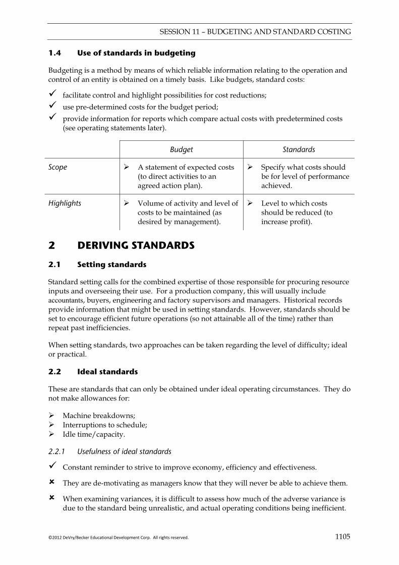
SESSION 11 – BUDGETING AND STANDARD COSTING
©2012 DeVry/Becker Educational Development Corp. All rights reserved. 1105
1.4 Use of standards in budgeting
Budgeting is a method by means of which reliable information relating to the operation and control of an entity is obtained on a timely basis. Like budgets, standard costs:
facilitate control and highlight possibilities for cost reductions; use pre-determined costs for the budget period; provide information for reports which compare actual costs with predetermined costs
(see operating statements later).
Budget Standards
Scope A statement of expected costs (to direct activities to an agreed action plan).
Specify what costs should be for level of performance achieved.
Highlights Volume of activity and level of costs to be maintained (as desired by management).
Level to which costs should be reduced (to increase profit).
2 DERIVING STANDARDS
2.1 Setting standards
Standard setting calls for the combined expertise of those responsible for procuring resource inputs and overseeing their use. For a production company, this will usually include accountants, buyers, engineering and factory supervisors and managers. Historical records provide information that might be used in setting standards. However, standards should be set to encourage efficient future operations (so not attainable all of the time) rather than repeat past inefficiencies.
When setting standards, two approaches can be taken regarding the level of difficulty; ideal or practical.
2.2 Ideal standards
These are standards that can only be obtained under ideal operating circumstances. They do not make allowances for:
Machine breakdowns; Interruptions to schedule; Idle time/capacity.
2.2.1 Usefulness of ideal standards
Constant reminder to strive to improve economy, efficiency and effectiveness.
They are de-motivating as managers know that they will never be able to achieve them.
When examining variances, it is difficult to assess how much of the adverse variance is due to the standard being unrealistic, and actual operating conditions being inefficient.
SESSION 11 – BUDGETING AND STANDARD COSTING
1106 ©2012 DeVry/Becker Educational Development Corp. All rights reserved.
2.3 Practical standards
Practical standards are challenging but should be attainable under existing operating conditions. They do make an allowance for a normal (i.e. expected) level of:
Machine breakdowns; Breaks (rests) by workforce.
On the other hand, they do require a high, though reasonable, level of efficiency. Practical standards are more likely to be used than ideal because:
They are achievable so managers will be motivated.
Any variances will highlight only abnormal conditions for the attention of management. This is useful for assisting in “management by exception”.
2.4 Information used for setting standards
In setting standards, for each input used, two standards have to be determined; the price per unit of input (kgs, hours) and the quantity used per unit of output. The following methods might be used for setting these:
2.4.1 Price per unit of input
The price is normally set to reflect current market prices for the budgeted period. The difficulty with prices is that they may change due to external factors. A solution to this is that the budget or standard may be revised prior to performing variance analysis to take this into account. Revisions of budgets are dealt with in a later session.
2.4.2 Quantity of materials
Quantity may be determined by a “Bill of materials” prepared by product design or engineering department or works foreman.
Allowance may also be made for an expected level of waste.
2.4.3 Direct labour hours
“Time and motion” studies of operations may be used to determine the most efficient production method.
Time measurements determine standard hours for the average worker to complete a job.
2.4.4 Wage rates
Wage rates are determined by company policy/negotiations between management and unions. Sometimes standards may have to be set before the annual wage negotiations have been concluded.
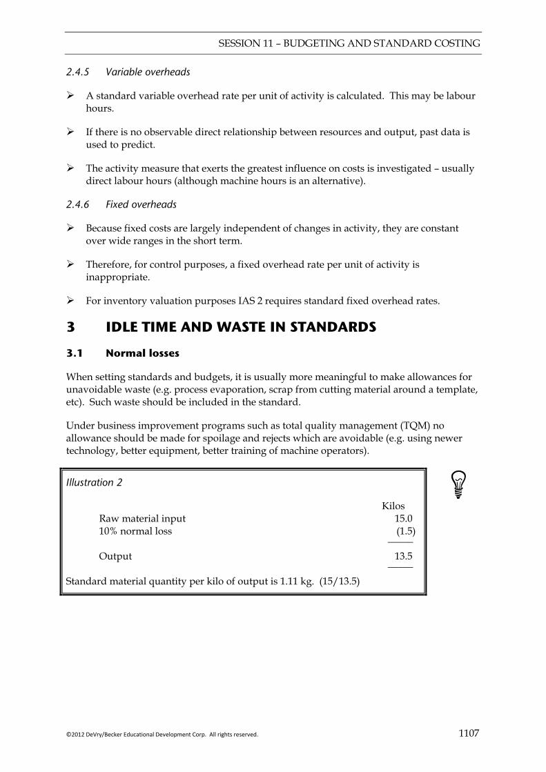
SESSION 11 – BUDGETING AND STANDARD COSTING
©2012 DeVry/Becker Educational Development Corp. All rights reserved. 1107
2.4.5 Variable overheads
A standard variable overhead rate per unit of activity is calculated. This may be labour hours.
If there is no observable direct relationship between resources and output, past data is used to predict.
The activity measure that exerts the greatest influence on costs is investigated – usually direct labour hours (although machine hours is an alternative).
2.4.6 Fixed overheads
Because fixed costs are largely independent of changes in activity, they are constant over wide ranges in the short term.
Therefore, for control purposes, a fixed overhead rate per unit of activity is inappropriate.
For inventory valuation purposes IAS 2 requires standard fixed overhead rates.
3 IDLE TIME AND WASTE IN STANDARDS
3.1 Normal losses
When setting standards and budgets, it is usually more meaningful to make allowances for unavoidable waste (e.g. process evaporation, scrap from cutting material around a template, etc). Such waste should be included in the standard.
Under business improvement programs such as total quality management (TQM) no allowance should be made for spoilage and rejects which are avoidable (e.g. using newer technology, better equipment, better training of machine operators).
Illustration 2
Kilos Raw material input 15.0 10% normal loss (1.5) _____
Output 13.5 _____
Standard material quantity per kilo of output is 1.11 kg. (15/13.5)
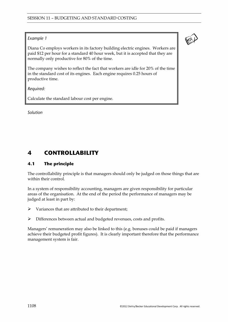
SESSION 11 – BUDGETING AND STANDARD COSTING
1108 ©2012 DeVry/Becker Educational Development Corp. All rights reserved.
Example 1
Diana Co employs workers in its factory building electric engines. Workers are paid $12 per hour for a standard 40 hour week, but it is accepted that they are normally only productive for 80% of the time.
The company wishes to reflect the fact that workers are idle for 20% of the time in the standard cost of its engines. Each engine requires 0.25 hours of productive time.
Required:
Calculate the standard labour cost per engine.
Solution
4 CONTROLLABILITY
4.1 The principle
The controllability principle is that managers should only be judged on those things that are within their control.
In a system of responsibility accounting, managers are given responsibility for particular areas of the organisation. At the end of the period the performance of managers may be judged at least in part by:
Variances that are attributed to their department;
Differences between actual and budgeted revenues, costs and profits.
Managers’ remuneration may also be linked to this (e.g. bonuses could be paid if managers achieve their budgeted profit figures). It is clearly important therefore that the performance management system is fair.

SESSION 11 – BUDGETING AND STANDARD COSTING
©2012 DeVry/Becker Educational Development Corp. All rights reserved. 1109
Example 2
Ron is the production manager of a factory making ball bearings. His performance is judged using variance analysis. The variance analysis for the last month has just been performed, and includes the following:
An adverse materials price variance due to a change in the supplier. The supplier was changed because the production manager complained that the quality of the products sold by the old supplier were sub-standard.
A labour idle time variance caused by two factors:
A strike lasting two days over pay.
A machine break down, meaning staff could not work until the machine was fixed.
A fixed overhead variance caused by an increase in factory rent. All rental contracts are dealt with by the company’s legal department.
Required:
Discuss which of the events above (if any) you think are outside of the control of Ron, and should therefore be ignored when assessing his performance.
Solution
5 FLEXED BUDGETS
5.1 Importance of flexed budgets
At the start of the year when a budget is prepared, estimates are made about the volume of sales and production. It is unlikely that the actual volume of sales and production will be the same as per the budget. This makes it difficult to compare actual performance against the budget, as they are based on different levels of activity.
The budget can be flexed at the end of the period before this comparison takes place. Flexing the budget simply means that the budget is recalculated based on the original budget assumptions (such as cost per unit, selling prices etc.) but based on the actual volume of sales and production. This flexed budget is then compared to the actual results. This results in a more valid comparison, as like is being compared with like.

SESSION 11 – BUDGETING AND STANDARD COSTING
1110 ©2012 DeVry/Becker Educational Development Corp. All rights reserved.
Finally three figures arise:
(1) Original budget (standard costs/revenues at expected activity level) (2) Flexed budget (standard costs/revenues at actual activity level) (3) Actual results
Volume variances
Other variances
Illustration 3
The following are extracts from a firm’s budgeted and actual results:
Budgeted production 100 units Budgeted materials cost per unit $5 Actual production 200 units Actual materials cost per unit $4
The three relevant figures here are as follows:
Original budget 100 × $5 = $500 Flexed budget 200 × $5 = $1,000 Actual cost 200 × $4 = $800
The $500 difference between the original budget and the flexed budget reflects the additional expected cost due to the fact that the volume of activity was higher than expected. The $200 difference between the flexed budget and the actual cost reflects the fact that $200 less has been spent on materials than would be expected given the volume of activity. This variance is the more useful assessment of performance.
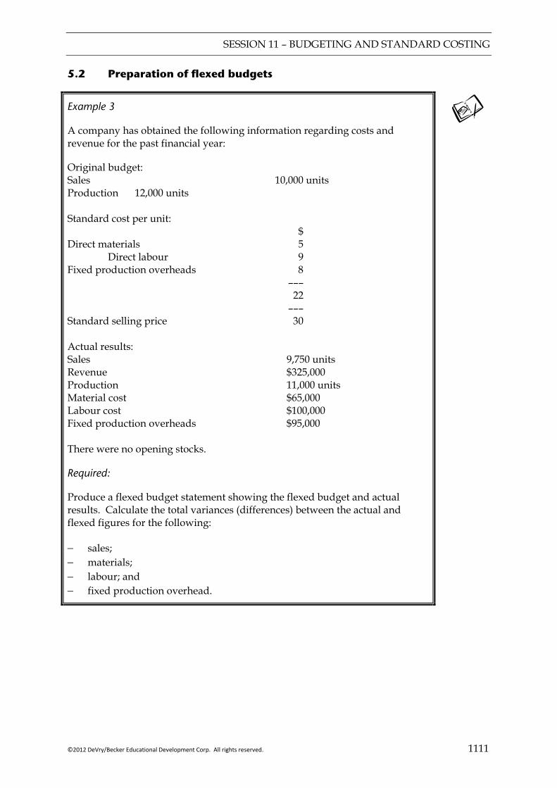
SESSION 11 – BUDGETING AND STANDARD COSTING
©2012 DeVry/Becker Educational Development Corp. All rights reserved. 1111
5.2 Preparation of flexed budgets
Example 3
A company has obtained the following information regarding costs and revenue for the past financial year:
Original budget: Sales 10,000 units Production 12,000 units Standard cost per unit: $ Direct materials 5
Direct labour 9 Fixed production overheads 8 ––– 22 ––– Standard selling price 30 Actual results: Sales 9,750 units Revenue $325,000 Production 11,000 units Material cost $65,000 Labour cost $100,000 Fixed production overheads $95,000 There were no opening stocks.
Required:
Produce a flexed budget statement showing the flexed budget and actual results. Calculate the total variances (differences) between the actual and flexed figures for the following:
− sales; − materials; − labour; and − fixed production overhead.
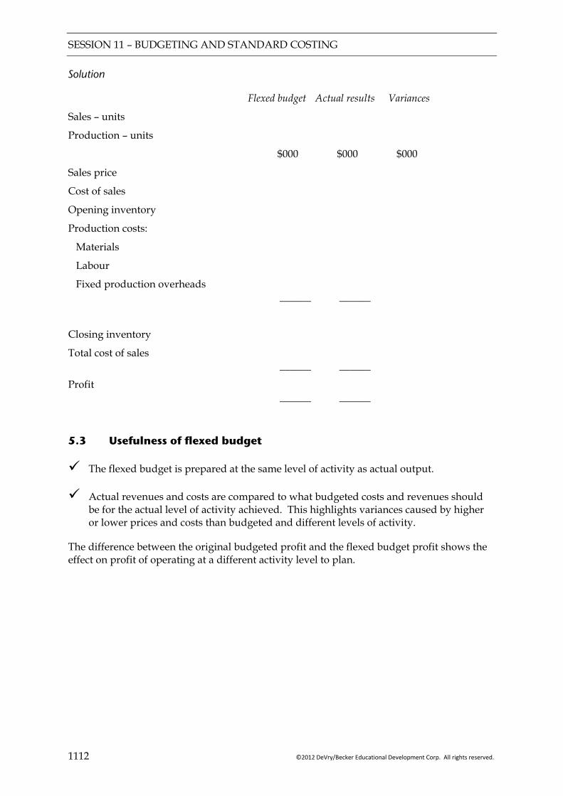
SESSION 11 – BUDGETING AND STANDARD COSTING
1112 ©2012 DeVry/Becker Educational Development Corp. All rights reserved.
Solution
Flexed budget Actual results Variances
Sales – units
Production – units
$000 $000 $000
Sales price
Cost of sales
Opening inventory
Production costs:
Materials
Labour
Fixed production overheads ______ ______
Closing inventory
Total cost of sales ______ ______
Profit ______ ______
5.3 Usefulness of flexed budget
The flexed budget is prepared at the same level of activity as actual output.
Actual revenues and costs are compared to what budgeted costs and revenues should be for the actual level of activity achieved. This highlights variances caused by higher or lower prices and costs than budgeted and different levels of activity.
The difference between the original budgeted profit and the flexed budget profit shows the effect on profit of operating at a different activity level to plan.
SESSION 11 – BUDGETING AND STANDARD COSTING
©2012 DeVry/Becker Educational Development Corp. All rights reserved. 1113
Key points
A standard cost is a planned cost for a product or service. Actual costs are compared against the standard, and the resulting variances investigated to identify the cause. Thus standard costing is an important element in financial control.
Ideal standards may be set, that assume perfect operating efficiency. This is unlikely to be achieved in practice, and so the use of ideal standards is de-motivating. An alternative method is to set practical standards that are challenging but achievable under existing operating conditions.
Controllability principle is the principle that managers should only be evaluated on things that are within their control. Controllability is an important factor to take into account when using variance analysis to assess a manager.
Budgets may be “flexed” prior to comparison with actual results. Flexing a budget means re calculating the budget based on the original budget assumptions, at the actual level of activity.
FOCUS
You should now be able to:
explain the use of standard costs;
outline methods used to derive standard costs and discuss the different types of cost possible;
explain the importance of flexing budgets in performance management;
prepare budgets and standards that allow for waste and idle time;
explain the principle of controllability in the performance management system;
prepare a flexed budget and comment on its usefulness.
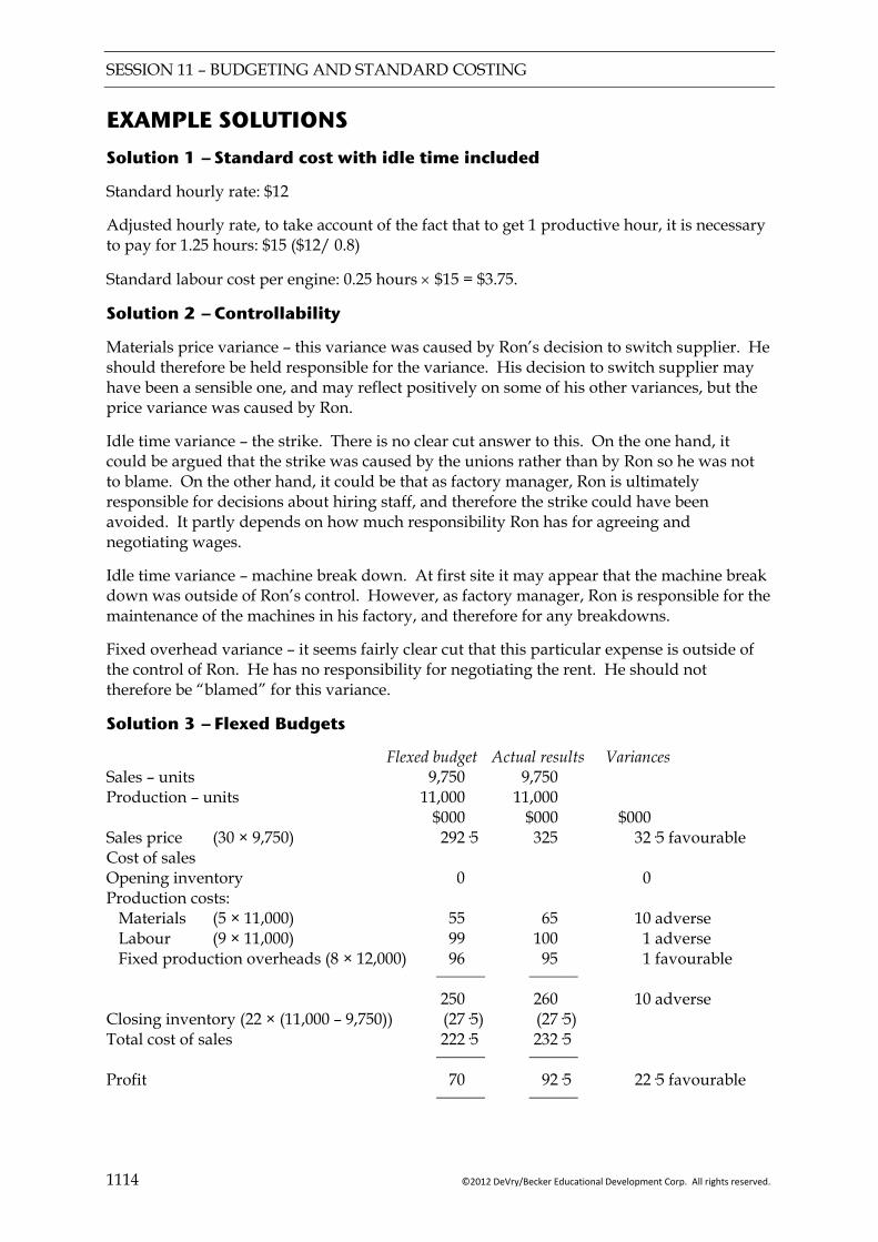
SESSION 11 – BUDGETING AND STANDARD COSTING
1114 ©2012 DeVry/Becker Educational Development Corp. All rights reserved.
EXAMPLE SOLUTIONS
Solution 1 — Standard cost with idle time included
Standard hourly rate: $12
Adjusted hourly rate, to take account of the fact that to get 1 productive hour, it is necessary to pay for 1.25 hours: $15 ($12/ 0.8)
Standard labour cost per engine: 0.25 hours × $15 = $3.75.
Solution 2 — Controllability
Materials price variance – this variance was caused by Ron’s decision to switch supplier. He should therefore be held responsible for the variance. His decision to switch supplier may have been a sensible one, and may reflect positively on some of his other variances, but the price variance was caused by Ron.
Idle time variance – the strike. There is no clear cut answer to this. On the one hand, it could be argued that the strike was caused by the unions rather than by Ron so he was not to blame. On the other hand, it could be that as factory manager, Ron is ultimately responsible for decisions about hiring staff, and therefore the strike could have been avoided. It partly depends on how much responsibility Ron has for agreeing and negotiating wages.
Idle time variance – machine break down. At first site it may appear that the machine break down was outside of Ron’s control. However, as factory manager, Ron is responsible for the maintenance of the machines in his factory, and therefore for any breakdowns.
Fixed overhead variance – it seems fairly clear cut that this particular expense is outside of the control of Ron. He has no responsibility for negotiating the rent. He should not therefore be “blamed” for this variance.
Solution 3 — Flexed Budgets
Flexed budget Actual results Variances Sales – units 9,750 9,750 Production – units 11,000 11,000 $000 $000 $000 Sales price (30 × 9,750) 292·5 325 32·5 favourable Cost of sales Opening inventory 0 0 Production costs: Materials (5 × 11,000) 55 65 10 adverse Labour (9 × 11,000) 99 100 1 adverse Fixed production overheads (8 × 12,000) 96 95 1 favourable ______ ______
250 260 10 adverse Closing inventory (22 × (11,000 – 9,750)) (27·5) (27·5) Total cost of sales 222·5 232·5 ______ ______
Profit 70 92·5 22·5 favourable ______ ______
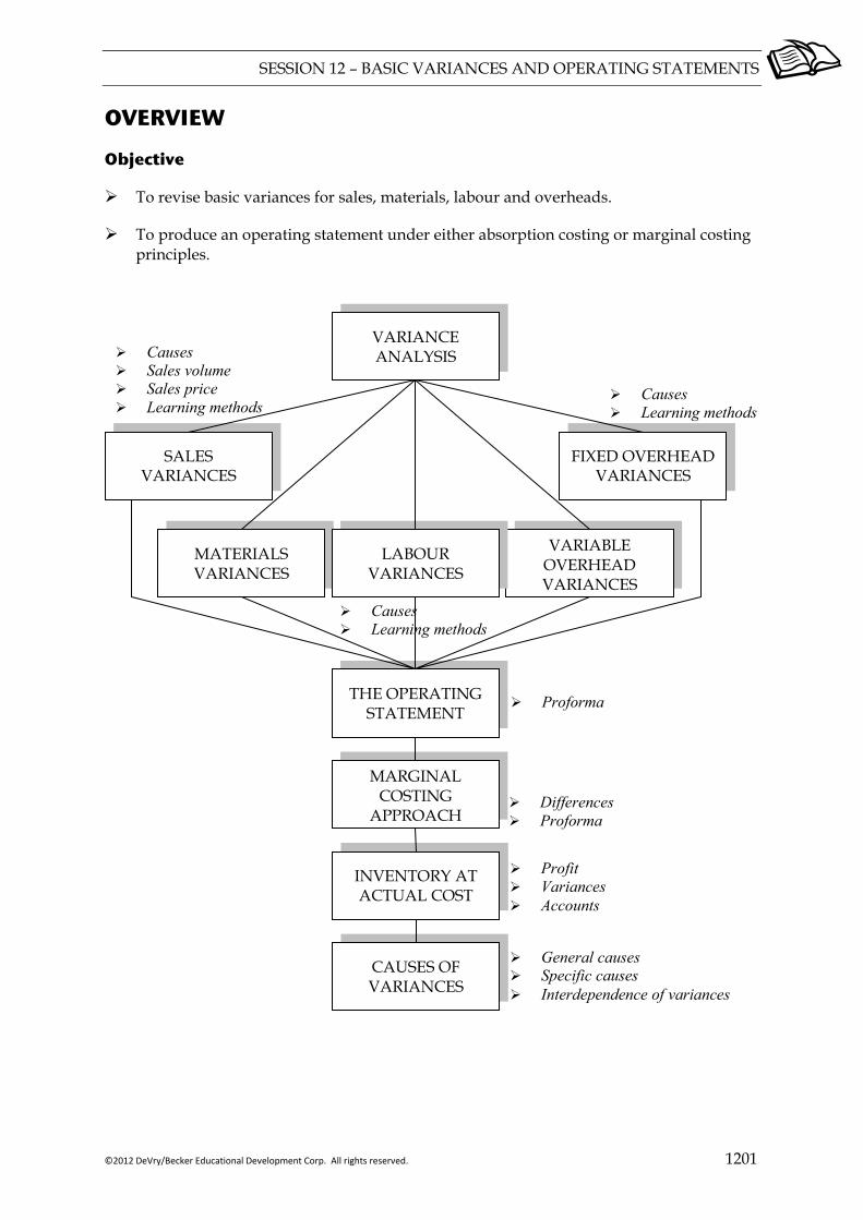
SESSION 12 – BASIC VARIANCES AND OPERATING STATEMENTS
©2012 DeVry/Becker Educational Development Corp. All rights reserved. 1201
OVERVIEW
Objective
To revise basic variances for sales, materials, labour and overheads.
To produce an operating statement under either absorption costing or marginal costing principles.
Causes Learning methods
VARIANCE ANALYSIS
FIXED OVERHEAD VARIANCES
SALES VARIANCES
MATERIALS VARIANCES
Causes Sales volume Sales price Learning methods
Profit Variances Accounts
VARIABLE OVERHEAD VARIANCES
LABOUR VARIANCES
Causes Learning methods
THE OPERATING STATEMENT
MARGINAL COSTING
APPROACH
INVENTORY AT ACTUAL COST
CAUSES OF VARIANCES
General causes Specific causes Interdependence of variances
Proforma
Differences Proforma
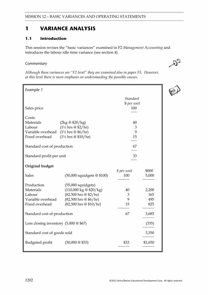
SESSION 12 – BASIC VARIANCES AND OPERATING STATEMENTS
1202 ©2012 DeVry/Becker Educational Development Corp. All rights reserved.
1 VARIANCE ANALYSIS
1.1 Introduction
This session revises the “basic variances” examined in F2 Management Accounting and introduces the labour idle time variance (see section 4).
Commentary Although these variances are “F2 level” they are examined also in paper F5. However, at this level there is more emphasis on understanding the possible causes.
Example 1
Standard $ per unit Sales price 100 ___
Costs: Materials (2kg @ $20/kg) 40 Labour (1½ hrs @ $2/hr) 3 Variable overhead (1½ hrs @ $6/hr) 9 Fixed overhead (1½ hrs @ $10/hr) 15 ___ Standard cost of production 67 ___ Standard profit per unit 33 ___ Original budget $ per unit $000 Sales (50,000 squidgets @ $100) 100 5,000 ______ ______ Production (55,000 squidgets) Materials (110,000 kg @ $20/kg) 40 2,200 Labour (82,500 hrs @ $2/hr) 3 165 Variable overhead (82,500 hrs @ $6/hr) 9 495 Fixed overhead (82,500 hrs @ $10/hr) 15 825 ______ ______ Standard cost of production 67 3,685 ______ Less closing inventory (5,000 @ $67) (335) ______ Standard cost of goods sold 3,350 ______ Budgeted profit (50,000 @ $33) $33 $1,650 ______ ______
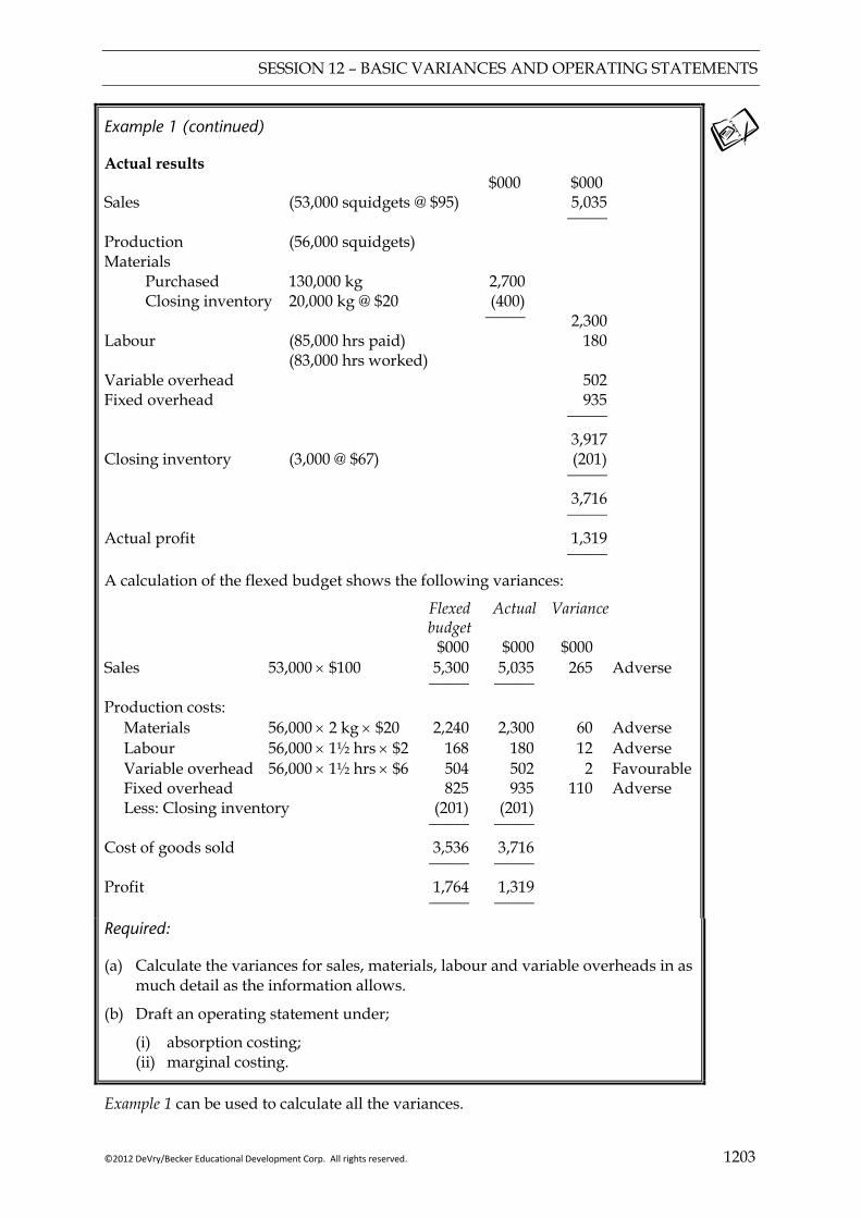
SESSION 12 – BASIC VARIANCES AND OPERATING STATEMENTS
©2012 DeVry/Becker Educational Development Corp. All rights reserved. 1203
Example 1 (continued)
Actual results $000 $000 Sales (53,000 squidgets @ $95) 5,035 _____
Production (56,000 squidgets) Materials
Purchased 130,000 kg 2,700 Closing inventory 20,000 kg @ $20 (400)
_____ 2,300 Labour (85,000 hrs paid) 180 (83,000 hrs worked) Variable overhead 502 Fixed overhead 935 _____ 3,917 Closing inventory (3,000 @ $67) (201) _____ 3,716 _____ Actual profit 1,319 _____ A calculation of the flexed budget shows the following variances:
Flexed Actual Variance budget $000 $000 $000 Sales 53,000 × $100 5,300 5,035 265 Adverse _____ _____ Production costs: Materials 56,000 × 2 kg × $20 2,240 2,300 60 Adverse Labour 56,000 × 1½ hrs × $2 168 180 12 Adverse Variable overhead 56,000 × 1½ hrs × $6 504 502 2 Favourable Fixed overhead 825 935 110 Adverse Less: Closing inventory (201) (201) _____ _____ Cost of goods sold 3,536 3,716 _____ _____ Profit 1,764 1,319 _____ _____
Required:
(a) Calculate the variances for sales, materials, labour and variable overheads in as much detail as the information allows.
(b) Draft an operating statement under;
(i) absorption costing; (ii) marginal costing.
Example 1 can be used to calculate all the variances.
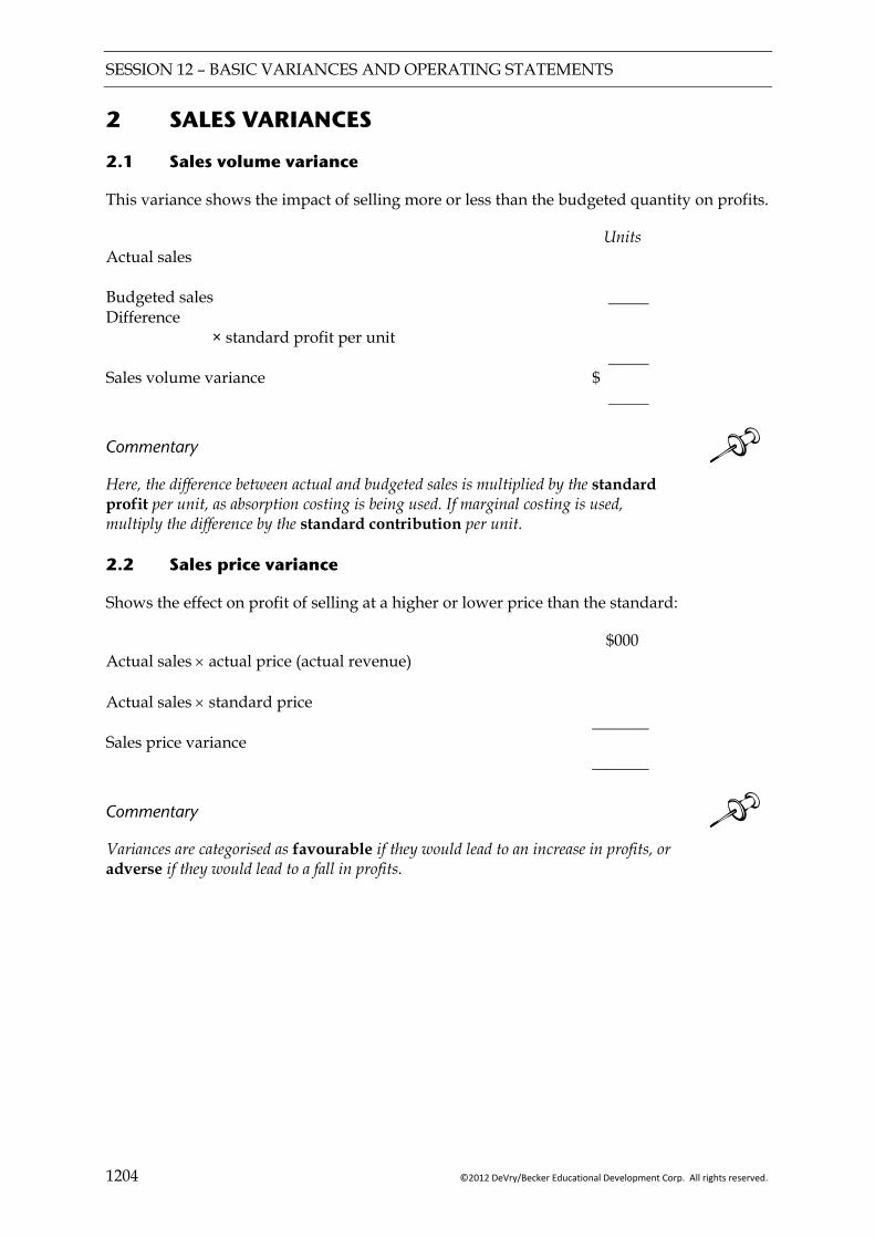
SESSION 12 – BASIC VARIANCES AND OPERATING STATEMENTS
1204 ©2012 DeVry/Becker Educational Development Corp. All rights reserved.
2 SALES VARIANCES
2.1 Sales volume variance
This variance shows the impact of selling more or less than the budgeted quantity on profits.
Units Actual sales Budgeted sales _____ Difference × standard profit per unit _____ Sales volume variance $ _____
Commentary Here, the difference between actual and budgeted sales is multiplied by the standard profit per unit, as absorption costing is being used. If marginal costing is used, multiply the difference by the standard contribution per unit.
2.2 Sales price variance
Shows the effect on profit of selling at a higher or lower price than the standard:
$000 Actual sales × actual price (actual revenue) Actual sales × standard price _______ Sales price variance _______
Commentary Variances are categorised as favourable if they would lead to an increase in profits, or adverse if they would lead to a fall in profits.
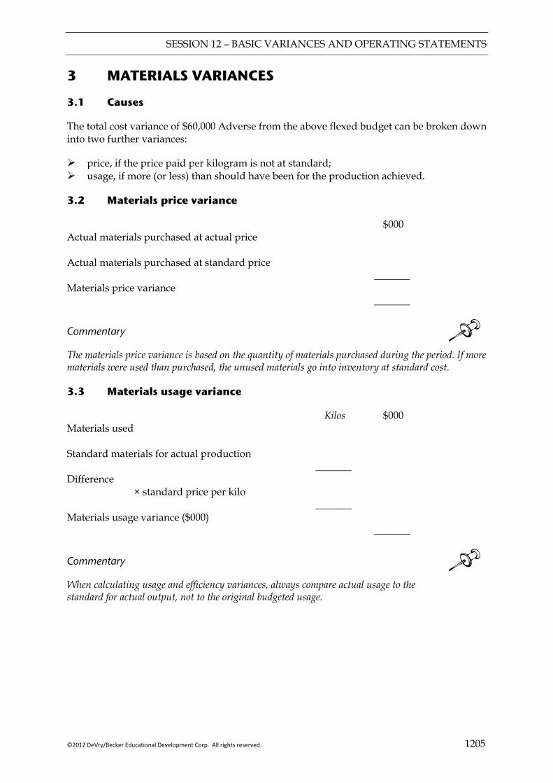
SESSION 12 – BASIC VARIANCES AND OPERATING STATEMENTS
©2012 DeVry/Becker Educational Development Corp. All rights reserved. 1205
3 MATERIALS VARIANCES
3.1 Causes
The total cost variance of $60,000 Adverse from the above flexed budget can be broken down into two further variances:
price, if the price paid per kilogram is not at standard; usage, if more (or less) than should have been for the production achieved.
3.2 Materials price variance
$000 Actual materials purchased at actual price Actual materials purchased at standard price _______ Materials price variance _______
Commentary The materials price variance is based on the quantity of materials purchased during the period. If more materials were used than purchased, the unused materials go into inventory at standard cost.
3.3 Materials usage variance
Kilos $000 Materials used Standard materials for actual production _______ Difference × standard price per kilo _______ Materials usage variance ($000) _______
Commentary When calculating usage and efficiency variances, always compare actual usage to the standard for actual output, not to the original budgeted usage.
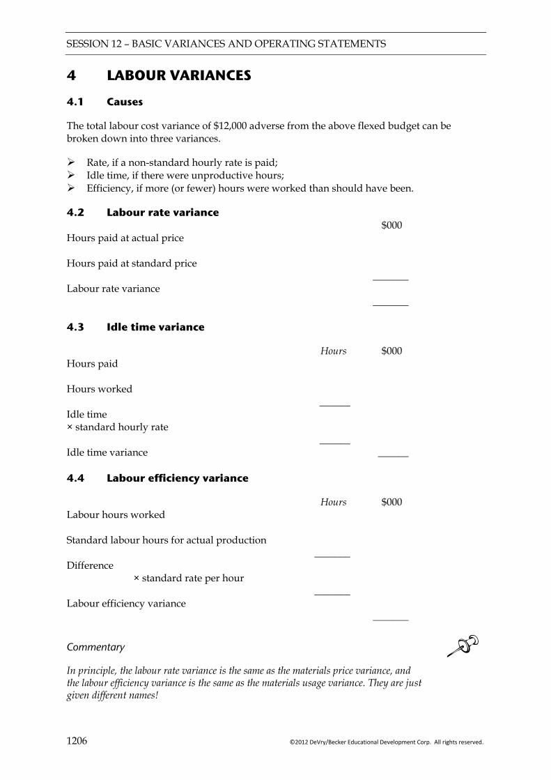
SESSION 12 – BASIC VARIANCES AND OPERATING STATEMENTS
1206 ©2012 DeVry/Becker Educational Development Corp. All rights reserved.
4 LABOUR VARIANCES
4.1 Causes
The total labour cost variance of $12,000 adverse from the above flexed budget can be broken down into three variances.
Rate, if a non-standard hourly rate is paid; Idle time, if there were unproductive hours; Efficiency, if more (or fewer) hours were worked than should have been.
4.2 Labour rate variance $000 Hours paid at actual price Hours paid at standard price _______ Labour rate variance _______ 4.3 Idle time variance
Hours $000 Hours paid Hours worked ______ Idle time × standard hourly rate ______ Idle time variance ______ 4.4 Labour efficiency variance
Hours $000 Labour hours worked Standard labour hours for actual production _______ Difference × standard rate per hour _______ Labour efficiency variance _______
Commentary In principle, the labour rate variance is the same as the materials price variance, and the labour efficiency variance is the same as the materials usage variance. They are just given different names!
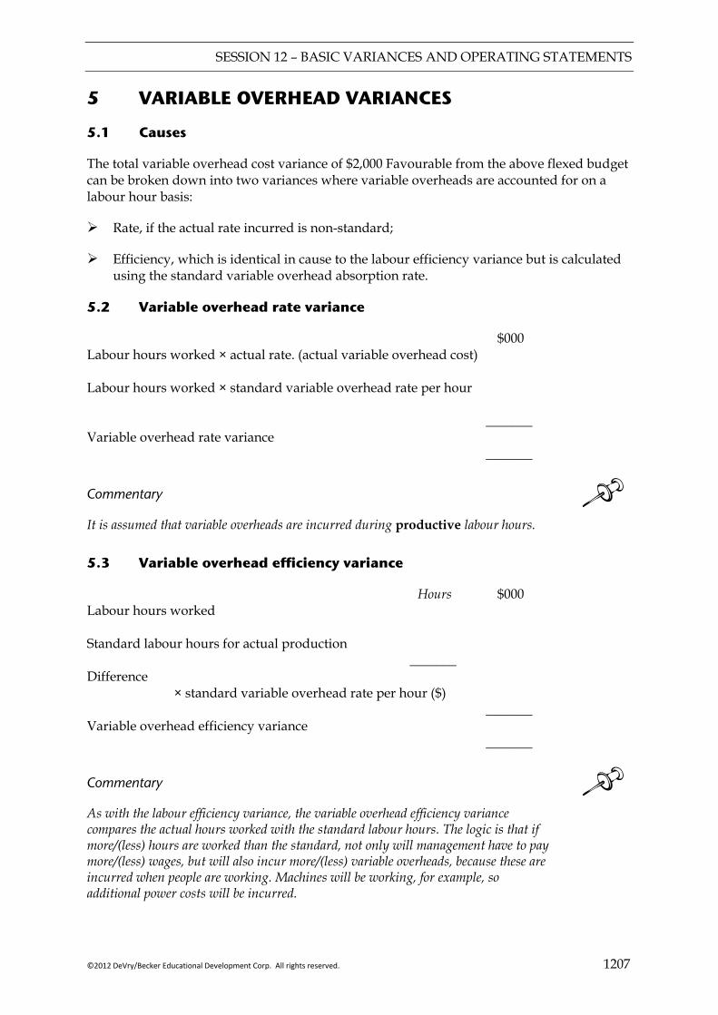
SESSION 12 – BASIC VARIANCES AND OPERATING STATEMENTS
©2012 DeVry/Becker Educational Development Corp. All rights reserved. 1207
5 VARIABLE OVERHEAD VARIANCES
5.1 Causes
The total variable overhead cost variance of $2,000 Favourable from the above flexed budget can be broken down into two variances where variable overheads are accounted for on a labour hour basis:
Rate, if the actual rate incurred is non-standard;
Efficiency, which is identical in cause to the labour efficiency variance but is calculated using the standard variable overhead absorption rate.
5.2 Variable overhead rate variance
$000 Labour hours worked × actual rate. (actual variable overhead cost) Labour hours worked × standard variable overhead rate per hour _______ Variable overhead rate variance _______
Commentary It is assumed that variable overheads are incurred during productive labour hours. 5.3 Variable overhead efficiency variance
Hours $000 Labour hours worked Standard labour hours for actual production _______ Difference × standard variable overhead rate per hour ($) _______ Variable overhead efficiency variance _______
Commentary As with the labour efficiency variance, the variable overhead efficiency variance compares the actual hours worked with the standard labour hours. The logic is that if more/(less) hours are worked than the standard, not only will management have to pay more/(less) wages, but will also incur more/(less) variable overheads, because these are incurred when people are working. Machines will be working, for example, so additional power costs will be incurred.
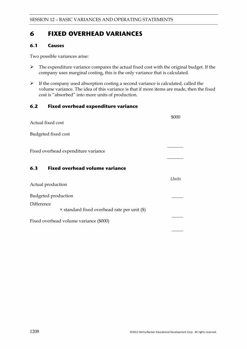
SESSION 12 – BASIC VARIANCES AND OPERATING STATEMENTS
1208 ©2012 DeVry/Becker Educational Development Corp. All rights reserved.
6 FIXED OVERHEAD VARIANCES
6.1 Causes
Two possible variances arise:
The expenditure variance compares the actual fixed cost with the original budget. If the company uses marginal costing, this is the only variance that is calculated.
If the company used absorption costing a second variance is calculated, called the volume variance. The idea of this variance is that if more items are made, then the fixed cost is “absorbed” into more units of production.
6.2 Fixed overhead expenditure variance
$000 Actual fixed cost Budgeted fixed cost _______ Fixed overhead expenditure variance _______ 6.3 Fixed overhead volume variance
Units Actual production Budgeted production _____
Difference × standard fixed overhead rate per unit ($) _____ Fixed overhead volume variance ($000)
_____
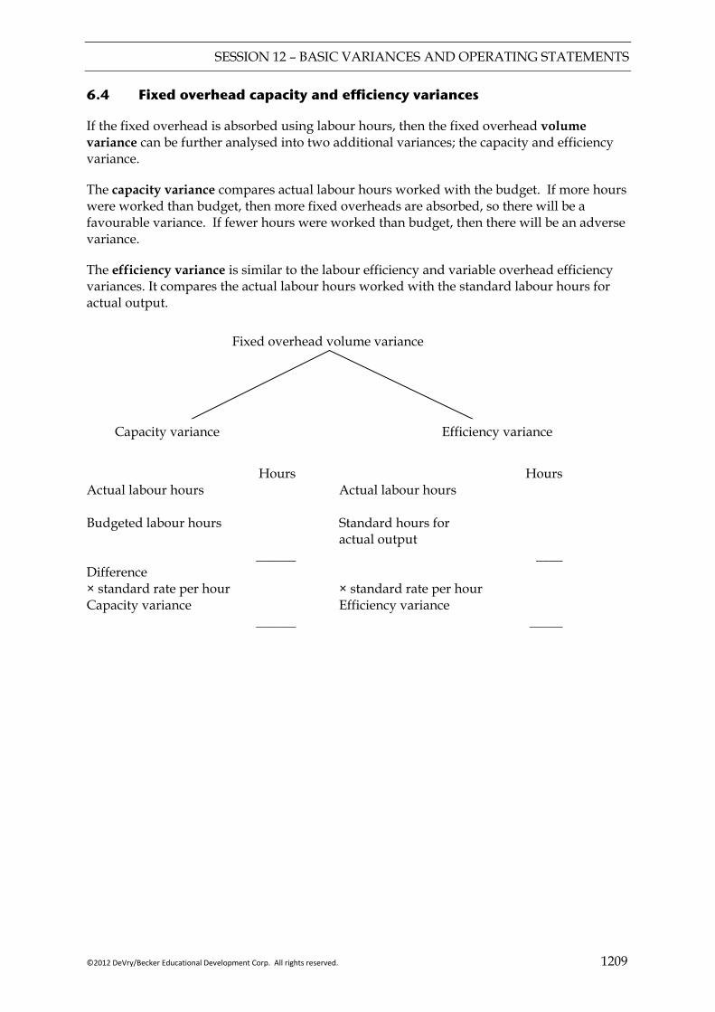
SESSION 12 – BASIC VARIANCES AND OPERATING STATEMENTS
©2012 DeVry/Becker Educational Development Corp. All rights reserved. 1209
6.4 Fixed overhead capacity and efficiency variances
If the fixed overhead is absorbed using labour hours, then the fixed overhead volume variance can be further analysed into two additional variances; the capacity and efficiency variance.
The capacity variance compares actual labour hours worked with the budget. If more hours were worked than budget, then more fixed overheads are absorbed, so there will be a favourable variance. If fewer hours were worked than budget, then there will be an adverse variance.
The efficiency variance is similar to the labour efficiency and variable overhead efficiency variances. It compares the actual labour hours worked with the standard labour hours for actual output.
Hours Hours Actual labour hours Actual labour hours Budgeted labour hours Standard hours for actual output ______ ____ Difference × standard rate per hour × standard rate per hour Capacity variance Efficiency variance ______ _____
Fixed overhead volume variance
Capacity variance Efficiency variance

SESSION 12 – BASIC VARIANCES AND OPERATING STATEMENTS
1210 ©2012 DeVry/Becker Educational Development Corp. All rights reserved.
7 THE OPERATING STATEMENT
7.1 Proforma
This summarises the earlier work and reconciles budgeted with actual profit.
For Example 1, a proforma statement follows:
Variance analysis proforma operating statement for the period ended
Favourable Adverse $000 $000 $000 Budgeted profit BQ × standard profit per unit 1,650 Sales margin variances Price (AP – SP) AQ Volume (AQ – BQ) standard profit per unit _____ _____ _____ Cost variances
Materials – price (SP – AP) AQp
– usage (SQ – AQu) SP
Labour – rate (SR – AR) AHp
– idle time (AHw – AHp) SR
– efficiency (SH – AHw) SR
Variable overhead
– rate (SR – AR) AHw
– efficiency (SH – AHw) SR
Fixed overhead
– expenditure budget – actual
– capacity (AHw – BH) SR
– efficiency (SH – AHw) SR
_____ _____
_____ _____ _____ Actual profit* 1,319 _____ * All inventories must be stated at standard absorption cost in determining actual profit.
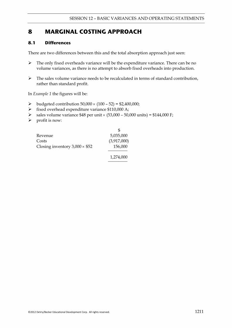
SESSION 12 – BASIC VARIANCES AND OPERATING STATEMENTS
©2012 DeVry/Becker Educational Development Corp. All rights reserved. 1211
8 MARGINAL COSTING APPROACH
8.1 Differences
There are two differences between this and the total absorption approach just seen:
The only fixed overheads variance will be the expenditure variance. There can be no volume variances, as there is no attempt to absorb fixed overheads into production.
The sales volume variance needs to be recalculated in terms of standard contribution, rather than standard profit.
In Example 1 the figures will be:
budgeted contribution 50,000 × (100 – 52) = $2,400,000; fixed overhead expenditure variance $110,000 A; sales volume variance $48 per unit × (53,000 – 50,000 units) = $144,000 F; profit is now:
$ Revenue 5,035,000 Costs (3,917,000) Closing inventory 3,000 × $52 156,000 _________ 1,274,000 _________
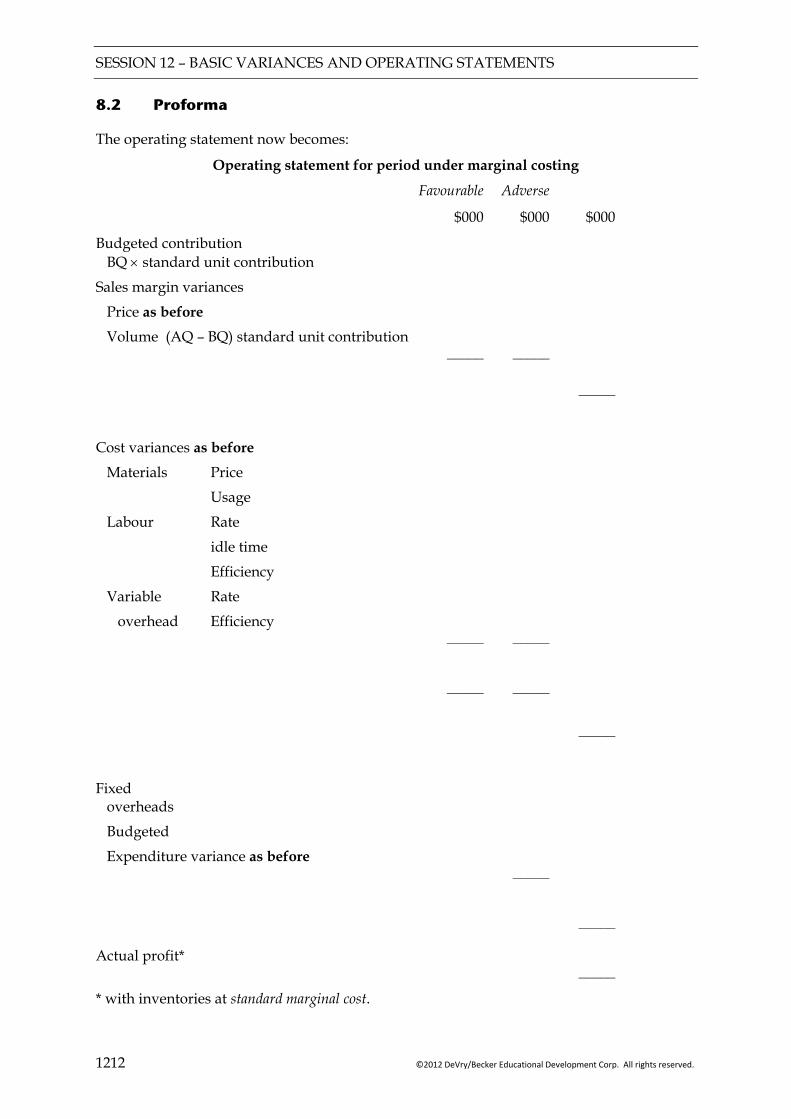
SESSION 12 – BASIC VARIANCES AND OPERATING STATEMENTS
1212 ©2012 DeVry/Becker Educational Development Corp. All rights reserved.
8.2 Proforma
The operating statement now becomes:
Operating statement for period under marginal costing
Favourable Adverse
$000 $000 $000
Budgeted contribution BQ × standard unit contribution
Sales margin variances
Price as before
Volume (AQ – BQ) standard unit contribution
_____ _____
_____
Cost variances as before
Materials Price
Usage
Labour Rate
idle time
Efficiency
Variable Rate
overhead Efficiency
_____ _____
_____ _____
_____
Fixed overheads
Budgeted
Expenditure variance as before
_____
_____
Actual profit*
_____
* with inventories at standard marginal cost.
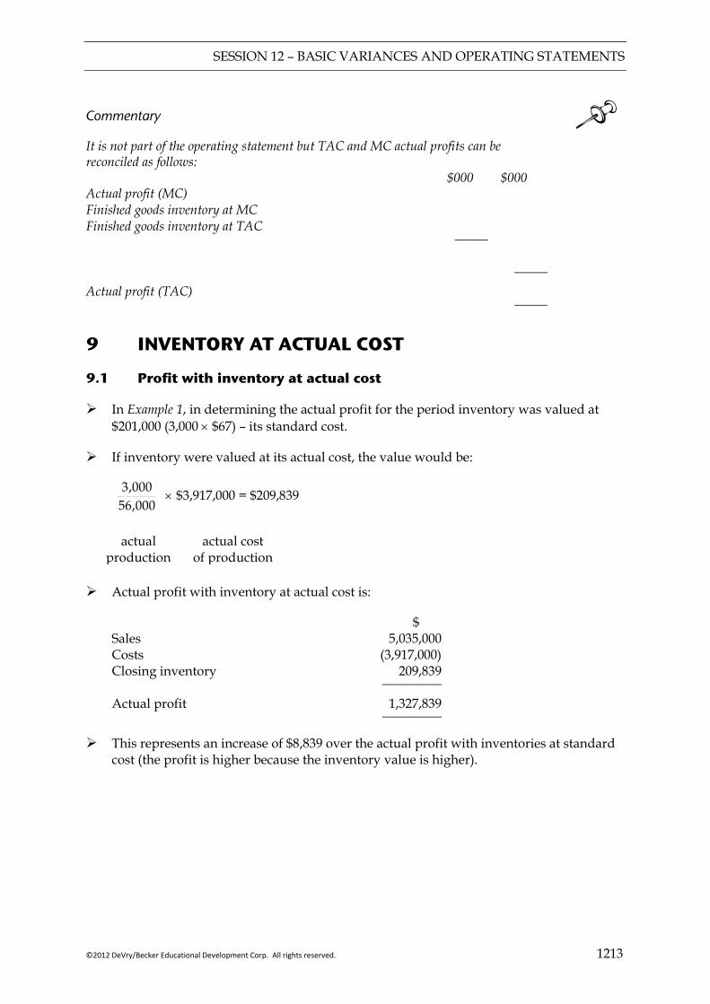
SESSION 12 – BASIC VARIANCES AND OPERATING STATEMENTS
©2012 DeVry/Becker Educational Development Corp. All rights reserved. 1213
Commentary It is not part of the operating statement but TAC and MC actual profits can be reconciled as follows:
$000 $000 Actual profit (MC) Finished goods inventory at MC Finished goods inventory at TAC _____ _____ Actual profit (TAC) _____ 9 INVENTORY AT ACTUAL COST
9.1 Profit with inventory at actual cost
In Example 1, in determining the actual profit for the period inventory was valued at $201,000 (3,000 × $67) – its standard cost.
If inventory were valued at its actual cost, the value would be:
000,56
000,3 × $3,917,000 = $209,839
actual
production actual cost
of production
Actual profit with inventory at actual cost is:
$ Sales 5,035,000 Costs (3,917,000) Closing inventory 209,839 _________
Actual profit 1,327,839 _________
This represents an increase of $8,839 over the actual profit with inventories at standard
cost (the profit is higher because the inventory value is higher).
SESSION 12 – BASIC VARIANCES AND OPERATING STATEMENTS
1214 ©2012 DeVry/Becker Educational Development Corp. All rights reserved.
9.2 Variances
$8,839 represents
000,56
000,3 × $165,000
total production cost variances
Commentary When inventory is valued at actual cost, some of the current period’s production cost variances are carried forward in the inventory value, rather than being expensed in profit or loss (which is what happens when inventory is valued at its standard cost).
9.3 Accounts
For internal (management control) purposes inventory is normally valued at its standard cost to highlight variances and to encourage any necessary remedial action to be taken.
For external financial reporting (e.g. annual accounts) inventory is normally valued at its actual cost.
10 CAUSES OF VARIANCES
10.1 General causes
Variances may be caused by:
planning errors (e.g. inaccurate standards); measurement errors (e.g. time recording errors); random factors (e.g. natural disasters); operational factors (e.g. management policies).
Operational factors may indicate that the process is out of control, and it is these which are considered below.
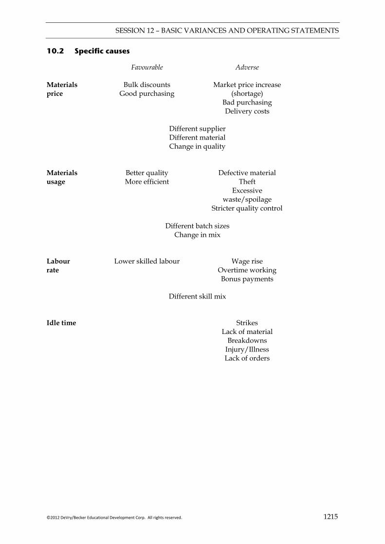
SESSION 12 – BASIC VARIANCES AND OPERATING STATEMENTS
©2012 DeVry/Becker Educational Development Corp. All rights reserved. 1215
10.2 Specific causes
Favourable Adverse Materials Bulk discounts Market price increase price Good purchasing (shortage) Bad purchasing Delivery costs Different supplier Different material Change in quality Materials Better quality Defective material usage More efficient Theft Excessive waste/spoilage Stricter quality control Different batch sizes Change in mix Labour Lower skilled labour Wage rise rate Overtime working Bonus payments Different skill mix Idle time Strikes Lack of material Breakdowns Injury/Illness Lack of orders

SESSION 12 – BASIC VARIANCES AND OPERATING STATEMENTS
1216 ©2012 DeVry/Becker Educational Development Corp. All rights reserved.
Favourable Adverse Labout Motivation Lower pay efficiency Higher pay Poor equipment Better equipment Slow working Learning effect Poor material Better material Lower grade Higher grade Overhead Cost savings/cutbacks Cost increases expenditure Excessive service usage Incorrect split of semi-variable and fixed costs Overhead See Labour efficiency efficiency Overhead Increase in productive Excessive idle time capacity hours Shortage of plant capacity Sales price Market shortage To achieve increase in volume Change in quality Response to competitors Pass on cost changes Sales Increase in market share Fall in market share volume Increase in market size Fall in market size
SESSION 12 – BASIC VARIANCES AND OPERATING STATEMENTS
©2012 DeVry/Becker Educational Development Corp. All rights reserved. 1217
10.3 Interdependence of variances
Frequently two or more opposing variances will be caused by the same operational factor.
It is necessary to consider the overall effect when considering any course of action.
10.3.1 Examples
Purchase high quality material:
adverse materials price; favourable materials usage.
Raise the selling price:
favourable sales price; adverse sales volume.
Use highly skilled labour:
adverse labour rate; favourable labour efficiency; favourable variable overhead efficiency; favourable fixed overhead efficiency.
10.3.2 A more complex example
Purchase high quality material:
adverse materials price; favourable materials usage; favourable labour efficiency; favourable variable overhead efficiency; favourable fixed overhead efficiency; favourable sales price; adverse sales volume.
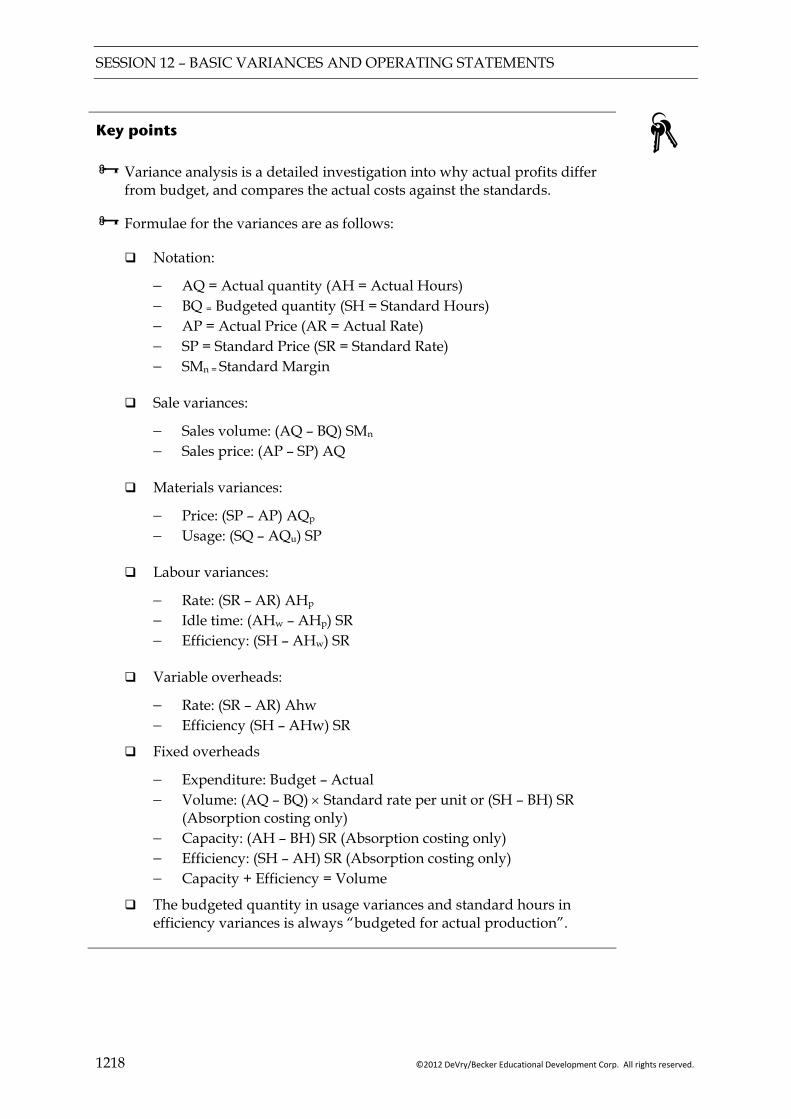
SESSION 12 – BASIC VARIANCES AND OPERATING STATEMENTS
1218 ©2012 DeVry/Becker Educational Development Corp. All rights reserved.
Key points
Variance analysis is a detailed investigation into why actual profits differ from budget, and compares the actual costs against the standards.
Formulae for the variances are as follows:
Notation:
− AQ = Actual quantity (AH = Actual Hours) − BQ = Budgeted quantity (SH = Standard Hours) − AP = Actual Price (AR = Actual Rate) − SP = Standard Price (SR = Standard Rate) − SMn = Standard Margin
Sale variances:
− Sales volume: (AQ – BQ) SMn − Sales price: (AP – SP) AQ
Materials variances:
− Price: (SP – AP) AQp − Usage: (SQ – AQu) SP
Labour variances:
− Rate: (SR – AR) AHp − Idle time: (AHw – AHp) SR − Efficiency: (SH – AHw) SR
Variable overheads:
− Rate: (SR – AR) Ahw − Efficiency (SH – AHw) SR
Fixed overheads
− Expenditure: Budget – Actual − Volume: (AQ – BQ) × Standard rate per unit or (SH – BH) SR
(Absorption costing only) − Capacity: (AH – BH) SR (Absorption costing only) − Efficiency: (SH – AH) SR (Absorption costing only) − Capacity + Efficiency = Volume
The budgeted quantity in usage variances and standard hours in efficiency variances is always “budgeted for actual production”.
SESSION 12 – BASIC VARIANCES AND OPERATING STATEMENTS
©2012 DeVry/Becker Educational Development Corp. All rights reserved. 1219
The only differences between variance analysis using absorption and marginal costing are:
Sales volume variance is valued at standard profit per unit for absorption, and standard contribution per unit for marginal.
There is only one fixed overhead variance for marginal costing; the expenditure overhead.
Variances could be caused by planning, measurement, random factors or operational factors. As far as investigating variances is concerned, it is operational factors which are more important.
FOCUS
You should now be able to:
calculate, identify the cause of and interpret basic variances:
sales price and volume;
materials total, price and usage;
labour total, rate and efficiency;
variable overhead total, expenditure and efficiency;
fixed overhead total, expenditure and efficiency and, where appropriate, volume, capacity and efficiency;
produce full operating statements in both a marginal cost and full absorption costing environment, reconciling actual profit to budgeted profit.

SESSION 12 – BASIC VARIANCES AND OPERATING STATEMENTS
1220 ©2012 DeVry/Becker Educational Development Corp. All rights reserved.
EXAMPLE SOLUTIONS
Solution 1 — Basic variances
(a) Variances
(i) Sales volume
Units Actual sales 53,000 Budgeted sales 50,000 ______ Difference 3,000 × standard profit per unit 33 _____ Sales volume variance $000 99 Favourable _____ (ii) Sales price
$000 Actual sales × actual price (actual revenue) 5,035 Actual sales × standard price (53,000 × 100) 5,300 _______ Sales price variance 265 Adverse _______ (iii) Materials price
$000 Actual materials purchased at actual price 2,700 Actual materials purchased at standard price (130,000 kg × $20) 2,600 _______ Materials price variance 100 Adverse _______ (iv) Materials usage
Kilos $000 Materials used (130,000 − 20,000) 110,000 Standard materials for actual production (56,000 units × 2kg) 112,000 _______ Difference 2,000 × standard price per kilo 20 _______ Materials usage variance ($000) 40 Favourable ___
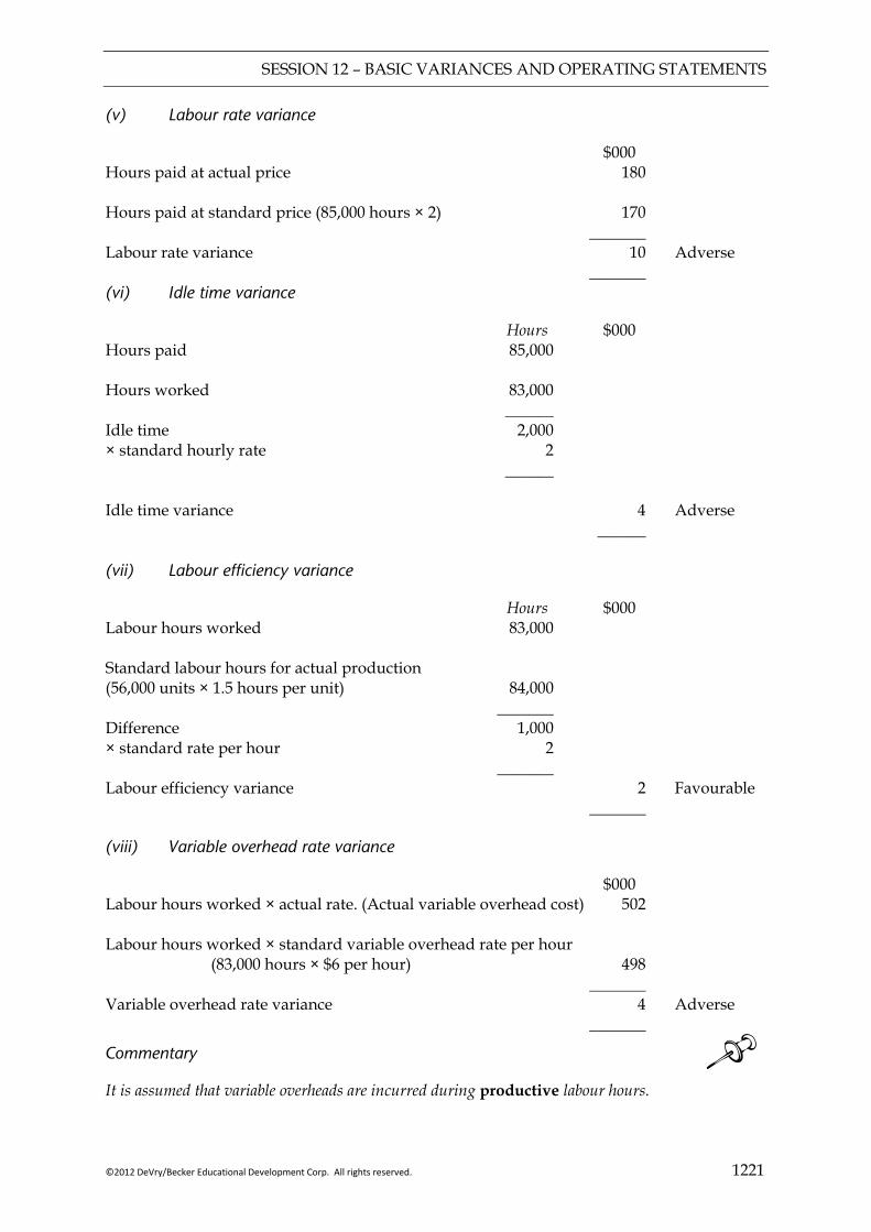
SESSION 12 – BASIC VARIANCES AND OPERATING STATEMENTS
©2012 DeVry/Becker Educational Development Corp. All rights reserved. 1221
(v) Labour rate variance
$000 Hours paid at actual price 180 Hours paid at standard price (85,000 hours × 2) 170 _______ Labour rate variance 10 Adverse _______ (vi) Idle time variance
Hours $000 Hours paid 85,000 Hours worked 83,000 ______ Idle time 2,000 × standard hourly rate 2 ______ Idle time variance 4 Adverse ______ (vii) Labour efficiency variance
Hours $000 Labour hours worked 83,000 Standard labour hours for actual production (56,000 units × 1.5 hours per unit) 84,000 _______ Difference 1,000 × standard rate per hour 2 _______ Labour efficiency variance 2 Favourable _______ (viii) Variable overhead rate variance
$000 Labour hours worked × actual rate. (Actual variable overhead cost) 502 Labour hours worked × standard variable overhead rate per hour (83,000 hours × $6 per hour) 498 _______ Variable overhead rate variance 4 Adverse _______
Commentary It is assumed that variable overheads are incurred during productive labour hours.
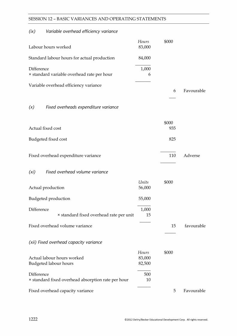
SESSION 12 – BASIC VARIANCES AND OPERATING STATEMENTS
1222 ©2012 DeVry/Becker Educational Development Corp. All rights reserved.
(ix) Variable overhead efficiency variance
Hours $000 Labour hours worked 83,000 Standard labour hours for actual production 84,000 _______ Difference 1,000 × standard variable overhead rate per hour 6 _______ Variable overhead efficiency variance 6 Favourable ___ (x) Fixed overheads expenditure variance
$000 Actual fixed cost 935 Budgeted fixed cost 825 _______ Fixed overhead expenditure variance 110 Adverse _______ (xi) Fixed overhead volume variance
Units $000 Actual production 56,000 Budgeted production 55,000 ______ Difference 1,000 × standard fixed overhead rate per unit 15 _____ Fixed overhead volume variance 15 favourable _____ (xii) Fixed overhead capacity variance
Hours $000 Actual labour hours worked 83,000 Budgeted labour hours 82,500 ______ Difference 500 × standard fixed overhead absorption rate per hour 10 ______ Fixed overhead capacity variance 5 Favourable
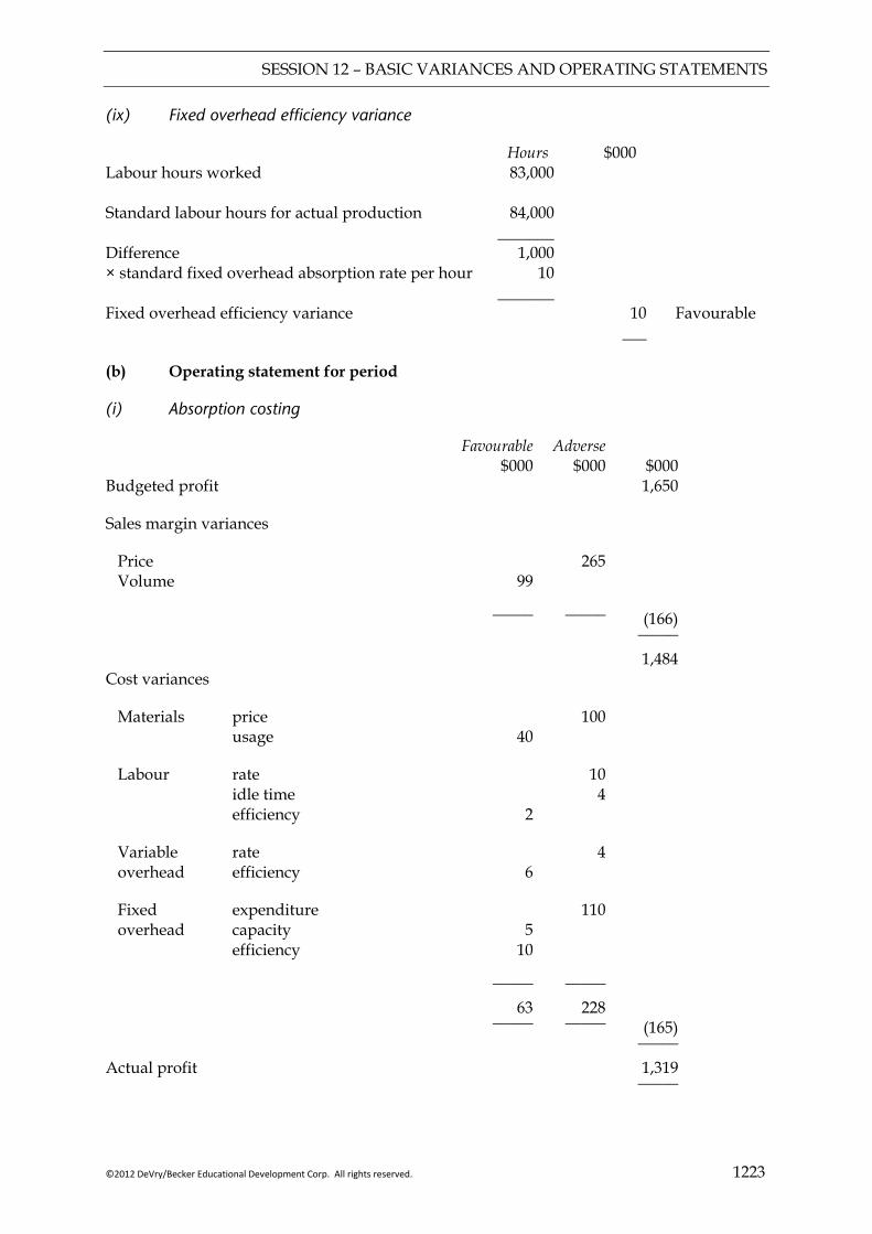
SESSION 12 – BASIC VARIANCES AND OPERATING STATEMENTS
©2012 DeVry/Becker Educational Development Corp. All rights reserved. 1223
(ix) Fixed overhead efficiency variance
Hours $000 Labour hours worked 83,000 Standard labour hours for actual production 84,000 _______ Difference 1,000 × standard fixed overhead absorption rate per hour 10 _______ Fixed overhead efficiency variance 10 Favourable ___ (b) Operating statement for period
(i) Absorption costing
Favourable Adverse $000 $000 $000 Budgeted profit 1,650
Sales margin variances
Price Volume
99
265
_____ _____ (166) _____ 1,484 Cost variances
Materials price usage
40
100
Labour rate idle time efficiency
2
10 4
Variable overhead
rate efficiency
6
4
Fixed overhead
expenditure capacity efficiency
5
10
110
_____ _____ 63 228 _____ _____ (165) Actual profit
_____ 1,319 _____
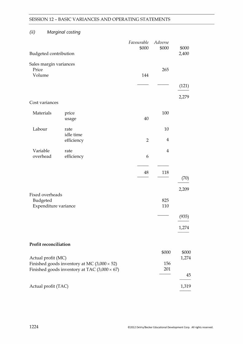
SESSION 12 – BASIC VARIANCES AND OPERATING STATEMENTS
1224 ©2012 DeVry/Becker Educational Development Corp. All rights reserved.
(ii) Marginal costing
Favourable Adverse $000 $000 $000 Budgeted contribution 2,400
Sales margin variances Price Volume
144
265
_____ _____ (121) _____ 2,279 Cost variances
Materials price usage
40
100
Labour rate idle time efficiency
2
10
4
Variable overhead
rate efficiency
6
4
_____ _____ 48 118 _____ _____ (70) _____ 2,209 Fixed overheads Budgeted Expenditure variance
825 110
_____ (935) _____
1,274 _____ Profit reconciliation
$000 $000 Actual profit (MC) Finished goods inventory at MC (3,000 × 52) Finished goods inventory at TAC (3,000 × 67)
156 201
1,274
_____ 45 Actual profit (TAC)
_____ 1,319 _____
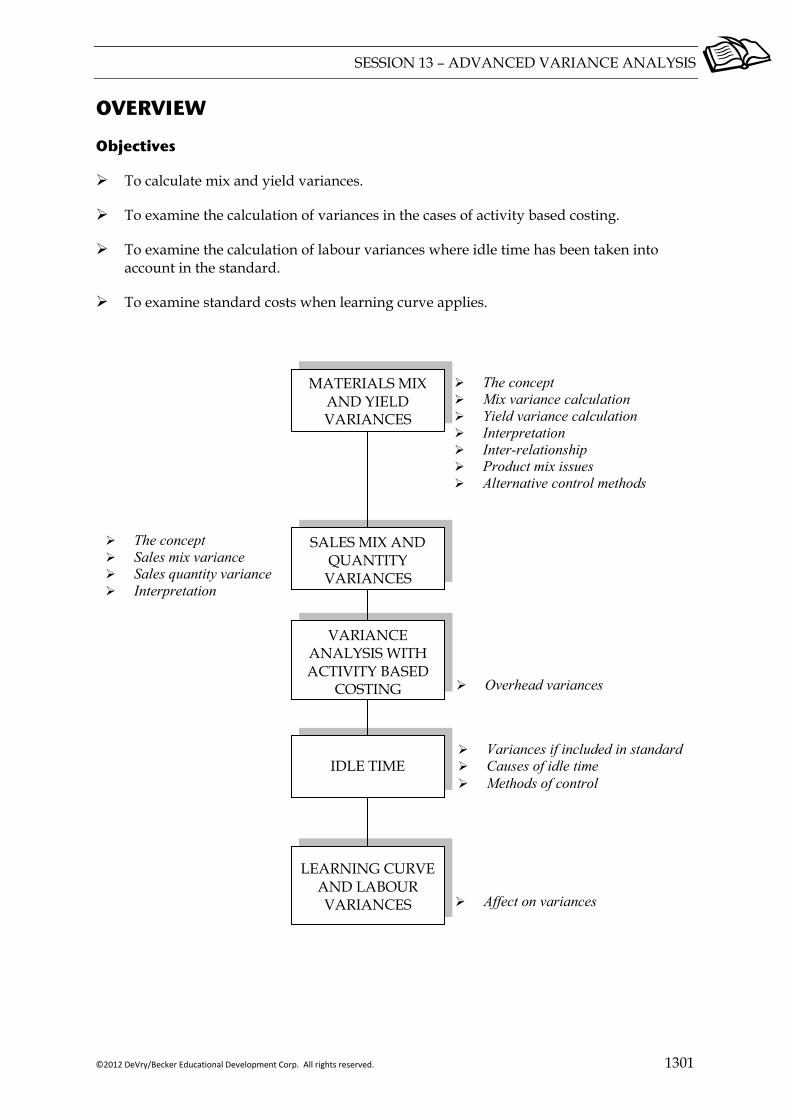
SESSION 13 – ADVANCED VARIANCE ANALYSIS
©2012 DeVry/Becker Educational Development Corp. All rights reserved. 1301
OVERVIEW
Objectives
To calculate mix and yield variances.
To examine the calculation of variances in the cases of activity based costing.
To examine the calculation of labour variances where idle time has been taken into account in the standard.
To examine standard costs when learning curve applies.
MATERIALS MIX AND YIELD VARIANCES
The concept Mix variance calculation Yield variance calculation Interpretation Inter-relationship Product mix issues Alternative control methods
The concept Sales mix variance Sales quantity variance Interpretation
SALES MIX AND QUANTITY
VARIANCES
VARIANCE ANALYSIS WITH ACTIVITY BASED
COSTING
IDLE TIME
LEARNING CURVE AND LABOUR VARIANCES
Overhead variances
Affect on variances
Variances if included in standard Causes of idle time Methods of control
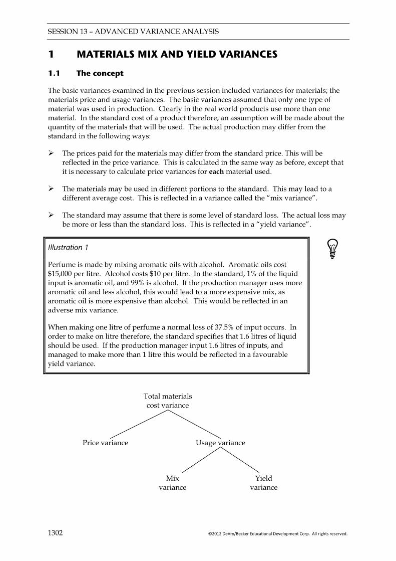
SESSION 13 – ADVANCED VARIANCE ANALYSIS
1302 ©2012 DeVry/Becker Educational Development Corp. All rights reserved.
1 MATERIALS MIX AND YIELD VARIANCES
1.1 The concept
The basic variances examined in the previous session included variances for materials; the materials price and usage variances. The basic variances assumed that only one type of material was used in production. Clearly in the real world products use more than one material. In the standard cost of a product therefore, an assumption will be made about the quantity of the materials that will be used. The actual production may differ from the standard in the following ways:
The prices paid for the materials may differ from the standard price. This will be reflected in the price variance. This is calculated in the same way as before, except that it is necessary to calculate price variances for each material used.
The materials may be used in different portions to the standard. This may lead to a different average cost. This is reflected in a variance called the “mix variance”.
The standard may assume that there is some level of standard loss. The actual loss may be more or less than the standard loss. This is reflected in a “yield variance”.
Illustration 1
Perfume is made by mixing aromatic oils with alcohol. Aromatic oils cost $15,000 per litre. Alcohol costs $10 per litre. In the standard, 1% of the liquid input is aromatic oil, and 99% is alcohol. If the production manager uses more aromatic oil and less alcohol, this would lead to a more expensive mix, as aromatic oil is more expensive than alcohol. This would be reflected in an adverse mix variance.
When making one litre of perfume a normal loss of 37.5% of input occurs. In order to make on litre therefore, the standard specifies that 1.6 litres of liquid should be used. If the production manager input 1.6 litres of inputs, and managed to make more than 1 litre this would be reflected in a favourable yield variance.
Total materials cost variance
Price variance Usage variance
Mix variance
Yield variance
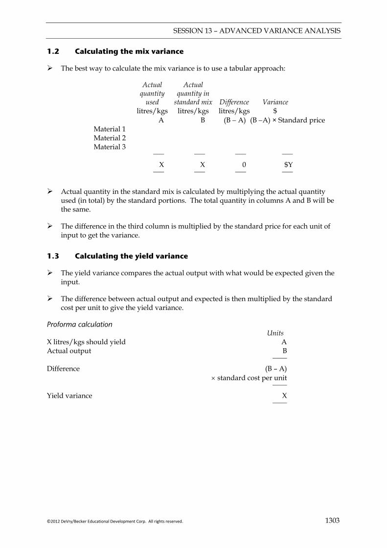
SESSION 13 – ADVANCED VARIANCE ANALYSIS
©2012 DeVry/Becker Educational Development Corp. All rights reserved. 1303
1.2 Calculating the mix variance
The best way to calculate the mix variance is to use a tabular approach:
Actual Actual quantity quantity in used standard mix Difference Variance litres/kgs litres/kgs litres/kgs $ A B (B − A) (B −A) × Standard price Material 1 Material 2 Material 3 ___ ___ ___ ___
X X 0 $Y ___ ___ ___ ___
Actual quantity in the standard mix is calculated by multiplying the actual quantity
used (in total) by the standard portions. The total quantity in columns A and B will be the same.
The difference in the third column is multiplied by the standard price for each unit of input to get the variance.
1.3 Calculating the yield variance
The yield variance compares the actual output with what would be expected given the input.
The difference between actual output and expected is then multiplied by the standard cost per unit to give the yield variance.
Proforma calculation Units X litres/kgs should yield A Actual output B ____
Difference (B – A) × standard cost per unit ____
Yield variance X ____

SESSION 13 – ADVANCED VARIANCE ANALYSIS
1304 ©2012 DeVry/Becker Educational Development Corp. All rights reserved.
Example 1
The standard material cost of a unit of a product is: $ Material X 2 kg @ $3 6 Material Y 1 kg @ $2 2 –––– –––– 3 kg 8 –––– ––––
The actual production was 5,000 units and the materials used were:
Material X 9,900 kg costing $27,000 Material Y 5,300 kg costing $11,000
Required:
Calculate the following variances:
(a) total materials cost; (b) materials price; (c) materials mix; (d) materials yield; (e) materials usage.
Solution
(a) Total materials cost variance
$
Standard cost of actual production
Actual cost of actual production
______ ______
(b) Materials price variance
Actual Actual quantity quantity at actual at standard price price Variance $ $ $ Material X 27,000 Y 11,000 ______ ______ ______
38,000 ______ ______ ______
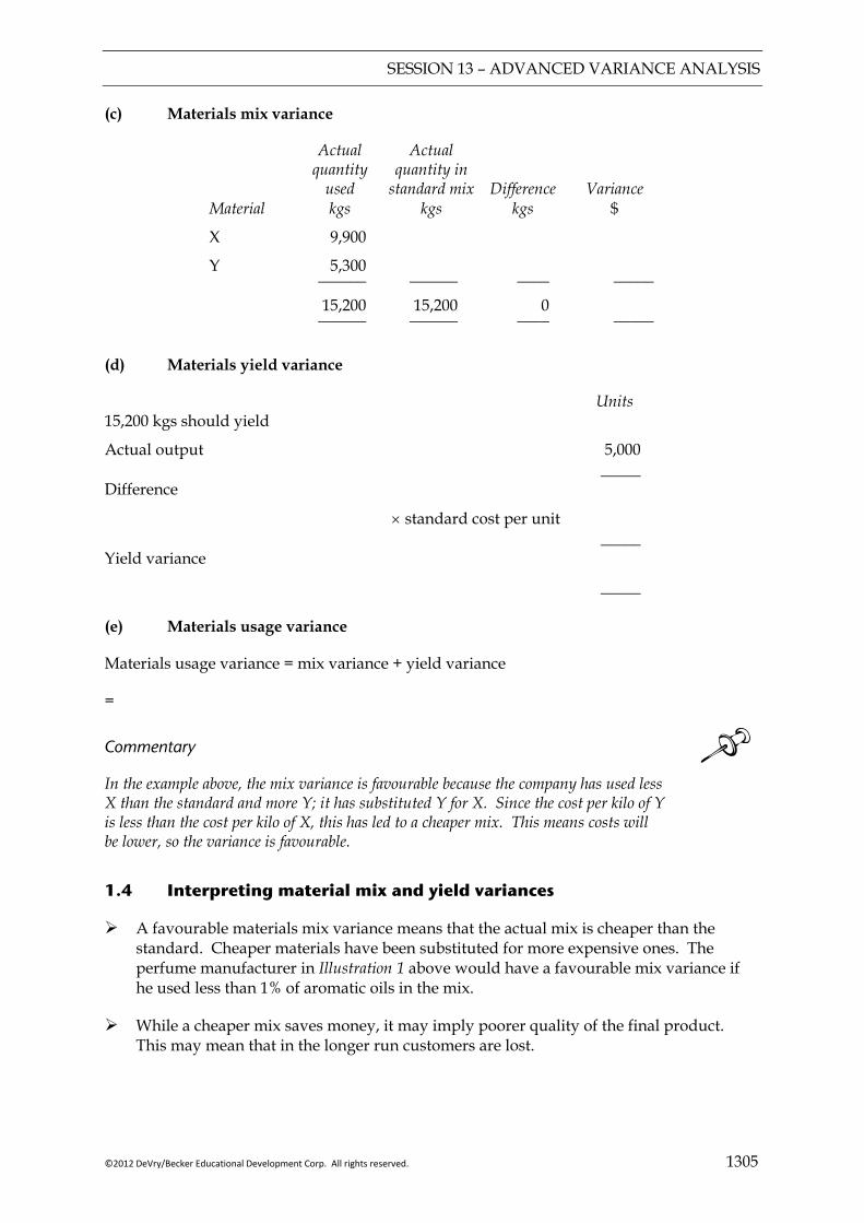
SESSION 13 – ADVANCED VARIANCE ANALYSIS
©2012 DeVry/Becker Educational Development Corp. All rights reserved. 1305
(c) Materials mix variance
Actual Actual quantity quantity in used standard mix Difference Variance Material kgs kgs kgs $
X 9,900
Y 5,300 ______ ______ ____ _____
15,200 15,200 0 ______ ______ ____ _____
(d) Materials yield variance
Units 15,200 kgs should yield
Actual output 5,000 _____ Difference
× standard cost per unit _____ Yield variance
_____ (e) Materials usage variance
Materials usage variance = mix variance + yield variance
=
Commentary In the example above, the mix variance is favourable because the company has used less X than the standard and more Y; it has substituted Y for X. Since the cost per kilo of Y is less than the cost per kilo of X, this has led to a cheaper mix. This means costs will be lower, so the variance is favourable.
1.4 Interpreting material mix and yield variances
A favourable materials mix variance means that the actual mix is cheaper than the standard. Cheaper materials have been substituted for more expensive ones. The perfume manufacturer in Illustration 1 above would have a favourable mix variance if he used less than 1% of aromatic oils in the mix.
While a cheaper mix saves money, it may imply poorer quality of the final product. This may mean that in the longer run customers are lost.
SESSION 13 – ADVANCED VARIANCE ANALYSIS
1306 ©2012 DeVry/Becker Educational Development Corp. All rights reserved.
Yield variance means that more output has been provided than expected, given the units input. This could be for one of the following reasons:
There is less spillage.
The manager has used more expensive, higher quality materials, which may mean that less is wasted than expected.
1.5 Inter-relationship between price, mix and yield variances
Price variance is something which may be outside of the control of the production manager. Prices may be seasonal, or based on a market rate, which it is not possible for the production manager to influence.
In some situations, managers may be able to obtain cheaper inputs by buying from alternative suppliers. This will result in favourable price variances. However, the cheaper materials may be of lower quality, and this may affect the yield variance, because more of the materials will be wasted.
Yield variance may be related to mix variance too; if the manager has used a cheaper mix of materials, this may lead to a lower output of products.
1.6 Wider issues relating to product mix
It is likely that for many products, it is possible to vary the portions of materials used, or to use a different materials mix to the standard.
Illustration 2
Imagine cooking a meal at home. Perhaps you are following a recipe from a cook book. Do you always weigh out the ingredients precisely, so that your mix is exactly the same as the cookbook (the standard)? Or perhaps you vary them slightly, based on your own personal taste, or perhaps simply because you do not measure everything precisely; you just roughly estimate how much you have put in. You know that you will still have a meal at the end and hopefully one that tastes good.
When the standard product mix was set, it is likely that the following issues were considered:
Balancing the mix and yield: It is often the case that using a cheaper “mix” of materials leads to a lower yield. The standard mix attempt to get the lowest cost per unit so that there is an economical mix of products with an acceptable yield.
Quality: A cheaper mix may lead to lower cost, but this may also lower the quality.

SESSION 13 – ADVANCED VARIANCE ANALYSIS
©2012 DeVry/Becker Educational Development Corp. All rights reserved. 1307
1.6.1 Reasons for varying the mix
In practice managers may move away from the standard mix for the following reasons:
The price of materials may change away from the standard, so one becomes relatively more expensive.
Inaccurate measurement of inputs due to careless ness or mistake
Intentionally using a cheaper mix to get a favourable mix variance.
1.6.2 Impact of varying the mix
A cheaper mix will lead to a favourable mix variance. However it is likely to have other adverse effects:
It may lead to a lower yield. When assessing the financial performance of the manager, the mix and yield variance need to be considered together. If the mix and yield variance added together yields an overall favourable variance, then from a financial perspective that may be considered to be good.
Poorer quality of output which is not reflected in variances. In the longer term, this will lead to a fall in sales. This will be reflected in an adverse sales volume variance, but it will take some time, so it may be that the adverse sales volume variance occurs in a later period.
Commentary It is always important to see the whole picture in exam questions. If the financial information is good (e.g. favourable mix and yield variance) what is the non-financial impact (e.g. on quality)?
1.7 Alternative methods of controlling production processes
Where production managers are evaluated on materials mix and yield variances, as we have seen above, they make take actions which would improve the measured variances, but at the expense of other important factors – particularly quality.
In order to overcome this, additional measures should be taken into account when assessing the performance of the managers. In particular, quality control measures. Measuring quality is not always easy, as this may be subjective.

SESSION 13 – ADVANCED VARIANCE ANALYSIS
1308 ©2012 DeVry/Becker Educational Development Corp. All rights reserved.
2 SALES MARGIN MIX AND QUANTITY VARIANCES
2.1 The concept
Basic calculations of sales price and volume variance were covered in the previous session.
Where the company sells more than one product, the budget will include the budgeted quantity of each product sold. The actual sales can be compared with the budget, and the sales volume variance calculated. The overall sales volume variance can be analysed into two further categories:
The sales margin mix variance (hereafter referred to as simply the sales mix variance) shows the impact on profit of selling a different “mix” to the standard. This implies that sales of the products may be related and that consumers decide to substitute sales of one product for another. If the products have different margins, then this will impact on profits.
The quantity variance compares the absolute quantity of goods sold in units with the budget. For this purpose, absolute quantity is assumed to occur in the standard mix.
Total sales variance
Price variance Volume variance
Mix variance
Quantity variance
2.2 Calculating the sales mix variance
The best way to calculate the sales mix variance is to use a table:
Actual Actual sales Standard Sales mix Product sales in budgeted Difference margin variance (units) mix (units) (units) $ $ X Y Z _____ ______ ______ ______ _____ ______ ______ ______ In principle the calculation of sales mix variance is very similar to the materials mix variance. Actual sales are compared with actual sales based on the budgeted sales mix. The difference is then multiplied by the standard margin per unit. Standard margin would normally be contribution per unit, although if absorption costing is used, standard profit per unit may be used. If in doubt, use standard contribution per unit.

SESSION 13 – ADVANCED VARIANCE ANALYSIS
©2012 DeVry/Becker Educational Development Corp. All rights reserved. 1309
2.3 Calculating the sales quantity variance
The starting point for the quantity variance is actual sales, adjusted to standard mix. This is then compared to budgeted sales, and the differences multiplied by the standard margin.
Actual Sales sales in Budgeted Standard quantity Product budgeted mix sales Difference margin variance (units) (units) (units) $ $ X Y Z _____ ______ ______ ______ _____ ______ ______ ______
Example 2
A company sells three related products; Q, P and R. Budgeted sales mix is 50% Q, and 25% for each of products P and R. The current periods budget and actual sales are shown below:
Products Budget Q P R Unit sales 200 100 100 Price $20 $25 $30 Margin $3 $4 $6 Actual Unit sales 180 150 170 Price $22 $22 $26 Required:
Calculate the sales price, mix and quantity variances.
Solution
Price variance $ Q
P
R _____ _____
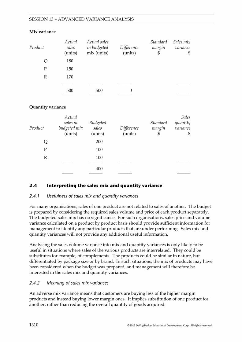
SESSION 13 – ADVANCED VARIANCE ANALYSIS
1310 ©2012 DeVry/Becker Educational Development Corp. All rights reserved.
Mix variance
Actual Actual sales Standard Sales mix Product sales in budgeted Difference margin variance (units) mix (units) (units) $ $
Q 180
P 150
R 170 _____ ______ ______ ______
500 500 0 _____ ______ ______ ______
Quantity variance
Actual Sales sales in Budgeted Standard quantity Product budgeted mix sales Difference margin variance (units) (units) (units) $ $
Q 200
P 100
R 100 _____ ______ ______ ______
400 _____ ______ ______ ______
2.4 Interpreting the sales mix and quantity variance
2.4.1 Usefulness of sales mix and quantity variances
For many organisations, sales of one product are not related to sales of another. The budget is prepared by considering the required sales volume and price of each product separately. The budgeted sales mix has no significance. For such organisations, sales price and volume variance calculated on a product by product basis should provide sufficient information for management to identify any particular products that are under performing. Sales mix and quantity variances will not provide any additional useful information.
Analysing the sales volume variance into mix and quantity variances is only likely to be useful in situations where sales of the various products are interrelated. They could be substitutes for example, of complements. The products could be similar in nature, but differentiated by package size or by brand. In such situations, the mix of products may have been considered when the budget was prepared, and management will therefore be interested in the sales mix and quantity variances.
2.4.2 Meaning of sales mix variances
An adverse mix variance means that customers are buying less of the higher margin products and instead buying lower margin ones. It implies substitution of one product for another, rather than reducing the overall quantity of goods acquired.
SESSION 13 – ADVANCED VARIANCE ANALYSIS
©2012 DeVry/Becker Educational Development Corp. All rights reserved. 1311
Illustration 3
A smoker decides to stop buying a premium brand of cigarettes and switches to a cheaper brand, but still continues to buy the same quantity of cigarettes. This would reduce the contribution of the tobacco company.
2.4.3 Meaning of sales quantity variance
The sales quantity variance shows the absolute quantity of goods sold against the budget. An adverse quantity variance may be due to poor economic conditions, or a new competitor. The sales quantity variance identifies factors that affect sales of all the products.
2.4.4 Interrelationships between the variances
The variances above are likely to be interrelated, so any analysis of variances should look at all the variances together rather than individually. Here are some ways in which they may be interrelated:
Sales price and sales volume variances: a fall in selling prices for products would lead to an adverse price variance. However, it may lead to higher demand for the products, so the volume variance would be favourable.
Sales mix and quantity variances: an adverse sales mix variance may be due to greater awareness of “better value” products, so customers may switch to these. For example, the company may offer packages that contain double the quantity of the product at less than twice the price of a standard sized package. Word may spread about these “better value” products, and other consumers may switch from competitors’ products, leading to a favourable quantity variance.
3 VARIANCE ANALYSIS WITH ACTIVITY BASED COSTING
3.1 Overhead variances
Where companies use activity based costing, the variances for labour and materials will remain unchanged. It is only the variances for overheads that may change.
Under activity based costing, overheads are absorbed based on drivers (see Session 2). The overhead element of a standard cost will make two assumptions:
number of products per unit of driver (e.g. number of items produced per machine hour); and
the standard cost per unit of driver.
Two variances may therefore be calculated:
An expenditure variance, which calculates the difference between the actual overhead cost and number of units of driver × standard cost per unit of driver;
An efficiency variance, which compares the number of units of driver actually used with the expected number of units, given actual output.
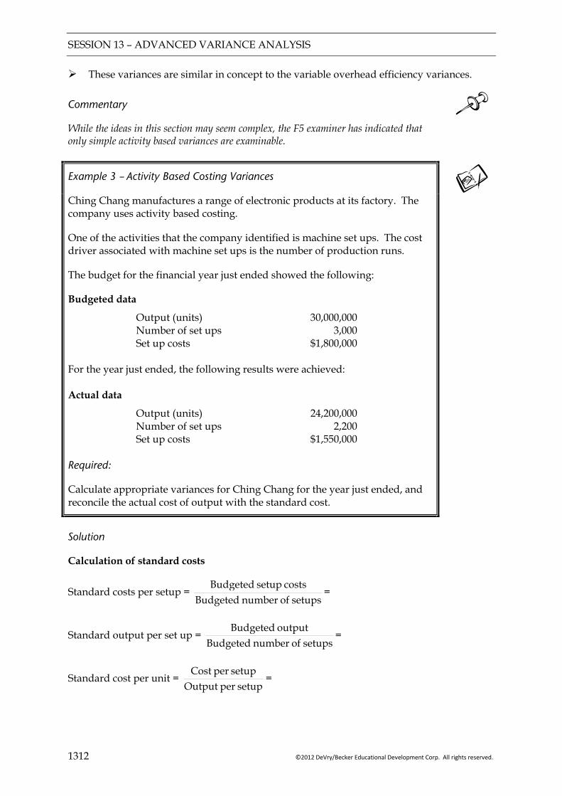
SESSION 13 – ADVANCED VARIANCE ANALYSIS
1312 ©2012 DeVry/Becker Educational Development Corp. All rights reserved.
These variances are similar in concept to the variable overhead efficiency variances.
Commentary While the ideas in this section may seem complex, the F5 examiner has indicated that only simple activity based variances are examinable.
Example 3 — Activity Based Costing Variances
Ching Chang manufactures a range of electronic products at its factory. The company uses activity based costing.
One of the activities that the company identified is machine set ups. The cost driver associated with machine set ups is the number of production runs.
The budget for the financial year just ended showed the following:
Budgeted data
Output (units) 30,000,000 Number of set ups 3,000 Set up costs $1,800,000 For the year just ended, the following results were achieved: Actual data
Output (units) 24,200,000 Number of set ups 2,200 Set up costs $1,550,000 Required:
Calculate appropriate variances for Ching Chang for the year just ended, and reconcile the actual cost of output with the standard cost.
Solution
Calculation of standard costs
Standard costs per setup = setups of number Budgeted
costs setup Budgeted=
Standard output per set up = setups of number Budgeted
output Budgeted=
Standard cost per unit = setup per Output
setup per Cost=
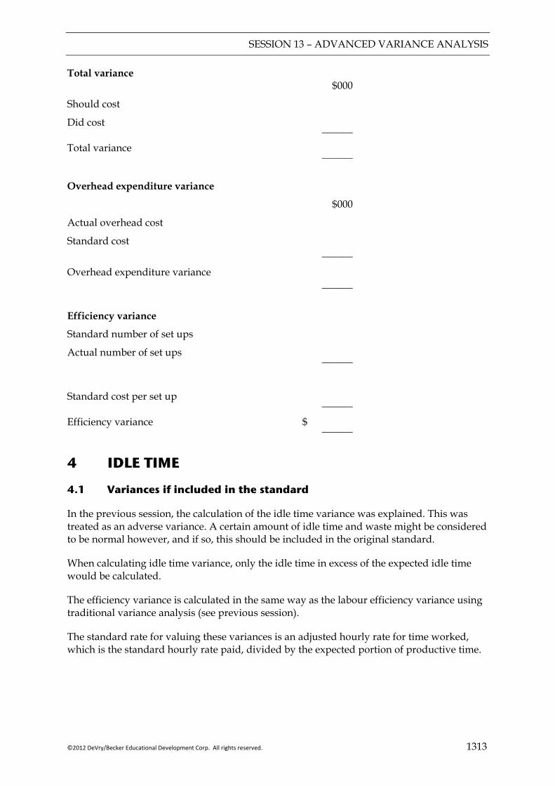
SESSION 13 – ADVANCED VARIANCE ANALYSIS
©2012 DeVry/Becker Educational Development Corp. All rights reserved. 1313
Total variance $000
Should cost
Did cost ______ Total variance ______ Overhead expenditure variance
$000
Actual overhead cost
Standard cost
______
Overhead expenditure variance
______
Efficiency variance
Standard number of set ups
Actual number of set ups ______
Standard cost per set up ______ Efficiency variance $ ______ 4 IDLE TIME
4.1 Variances if included in the standard
In the previous session, the calculation of the idle time variance was explained. This was treated as an adverse variance. A certain amount of idle time and waste might be considered to be normal however, and if so, this should be included in the original standard.
When calculating idle time variance, only the idle time in excess of the expected idle time would be calculated.
The efficiency variance is calculated in the same way as the labour efficiency variance using traditional variance analysis (see previous session).
The standard rate for valuing these variances is an adjusted hourly rate for time worked, which is the standard hourly rate paid, divided by the expected portion of productive time.
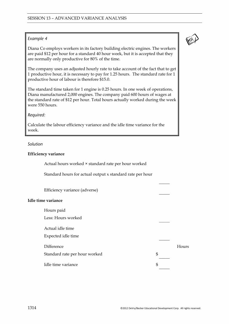
SESSION 13 – ADVANCED VARIANCE ANALYSIS
1314 ©2012 DeVry/Becker Educational Development Corp. All rights reserved.
Example 4
Diana Co employs workers in its factory building electric engines. The workers are paid $12 per hour for a standard 40 hour week, but it is accepted that they are normally only productive for 80% of the time.
The company uses an adjusted hourly rate to take account of the fact that to get 1 productive hour, it is necessary to pay for 1.25 hours. The standard rate for 1 productive hour of labour is therefore $15.0.
The standard time taken for 1 engine is 0.25 hours. In one week of operations, Diana manufactured 2,000 engines. The company paid 600 hours of wages at the standard rate of $12 per hour. Total hours actually worked during the week were 550 hours.
Required:
Calculate the labour efficiency variance and the idle time variance for the week.
Solution
Efficiency variance
Actual hours worked × standard rate per hour worked Standard hours for actual output x standard rate per hour _____
Efficiency variance (adverse) _____
Idle time variance
Hours paid
Less: Hours worked _____ Actual idle time
Expected idle time _____ Difference Hours
Standard rate per hour worked $ _____ Idle time variance $ _____
SESSION 13 – ADVANCED VARIANCE ANALYSIS
©2012 DeVry/Becker Educational Development Corp. All rights reserved. 1315
Commentary The efficiency variance is adverse, because the hours worked to achieve production of 2,000 engines was greater than expected, given the standard.
The idle time variance is favourable. Given that 600 hours were paid, we would expect idle time to be 20% of this, i.e. 120 hours. Idle time was actually only 50 hours.
4.2 Causes of idle time
Also called “downtime” and “dead time” reasons for it include:
Fall in demand for products reduces volume of production called for – workforce is waiting on orders being received;
Production stoppages (e.g. machine breakdown, industrial action (striking) by employee, stock-out of raw materials);
External factors (e.g. power surges or loss of power, natural disasters).
Poor production planning/scheduling resulting in employees waiting on one operation to be completed before another can be started.
Some idle time may be regarded as normal (e.g. stopping one operation and starting another) and cannot be wholly eliminated. Allowance for this should be made when calculating standard cost of direct labour.
Abnormal losses are not a direct labour cost – nor even a manufacturing overhead (to be absorbed in the cost of the product/service). Abnormal costs should always be written off directly to profit or loss and thereby highlighted for investigation:
Controllable idle time is that which could have been put to productive use (e.g. if management should have anticipated the situation and taken appropriate action);
Uncontrollable idle time (e.g. natural disaster).
4.3 Methods of control for idle time
Depending on the industry, idle time can be controlled and the cost of it reduced in a number of ways:
Improved production scheduling – to avoid bottlenecks;
Flexible workforce – to be able to lay-off excess when not needed;
Investment in equipment replacement and maintenance, including power generators – to reduce downtime;
Insurance for when disaster strikes.
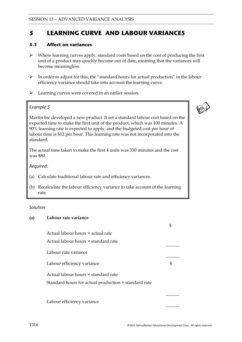
SESSION 13 – ADVANCED VARIANCE ANALYSIS
1316 ©2012 DeVry/Becker Educational Development Corp. All rights reserved.
5 LEARNING CURVE AND LABOUR VARIANCES
5.1 Affect on variances
Where learning curves apply, standard costs based on the cost of producing the first unit of a product may quickly become out of date, meaning that the variances will become meaningless.
In order to adjust for this, the “standard hours for actual production” in the labour efficiency variance should take into account the learning curve.
Learning curves were covered in an earlier session.
Example 5
Martin Inc developed a new product. It set a standard labour cost based on the expected time to make the first unit of the product, which was 100 minutes. A 90% learning rate is expected to apply, and the budgeted cost per hour of labour time is $12 per hour. This learning rate was not incorporated into the standard.
The actual time taken to make the first 4 units was 350 minutes and the cost was $80.
Required:
(a) Calculate traditional labour rate and efficiency variances.
(b) Recalculate the labour efficiency variance to take account of the learning rate.
Solution
(a) Labour rate variance
$
Actual labour hours × actual rate
Actual labour hours × standard rate ______
Labour rate variance ______ Labour efficiency variance $ Actual labour hours × standard rate
Standard hours for actual production × standard rate
______ Labour efficiency variance ______
SESSION 13 – ADVANCED VARIANCE ANALYSIS
©2012 DeVry/Becker Educational Development Corp. All rights reserved. 1317
(b) Recalculated labour efficiency variance
Actual labour hours × standard rate
Standard hours for actual production × standard rate (working) _____ Labour efficiency variance
_____ WORKING – standard hours for actual production taking into account the learning rate of 90%.
Output Cumulative Total (units) average time time 1
2
4
Key points
Materials mix variances measure the effect of using a different mix of inputs in the production process. Materials yield variances compare the output wit expected output, given the input and standard wastage.
Sale mix variances look at the impact of changing the mix of products on the contribution. Sales quantity variances look at the impact on selling a higher or lower quantity that budgeted.
Variance analysis can be performed in the case of activity based costing. An expenditure variance calculates the actual overhead cost with the standard cost for the amount of drivers used. An efficiency variance calculates the actual number of units of driver used and compares this with the standard number of units of driver, given actual output.
Where idle time is expected, standards may have been adjusted to take account of this. If this is the case, the idle time variance only takes into account idle time above expected idle time. Idle time and efficiency variances are also valued at an adjusted cost per productive hour, which takes into account the cost of the idle time required to obtain one unit of productive time.
Where learning curves exist, when calculating the standard cost of actual output, the learning rate should be taken into account rather than simply taking the standard cost of the first unit.
SESSION 13 – ADVANCED VARIANCE ANALYSIS
1318 ©2012 DeVry/Becker Educational Development Corp. All rights reserved.
FOCUS
You should now be able to:
calculate, identify the cause of, and explain mix and yield variances;
explain the wider issues involved in changing mix (e.g. cost, quality and performance measurement issues);
identify and explain the relationship of the material price variance with the material, mix and yield variances;
suggest and justify alternative methods of controlling production processes;
calculate, identify the cause of and explain sales mix and quantity variances;
identify and explain the relationship of the sales volume variances with the sales mix and quantity variances;
calculate using a simple situation, ABC-based variances;
calculate the effect of idle time and waste on variances including where idle time has been budgeted for;
explain the possible causes of idle time and waste and suggest methods of control;
explain the effect on labour variances where the learning curve has been used in the budget process.
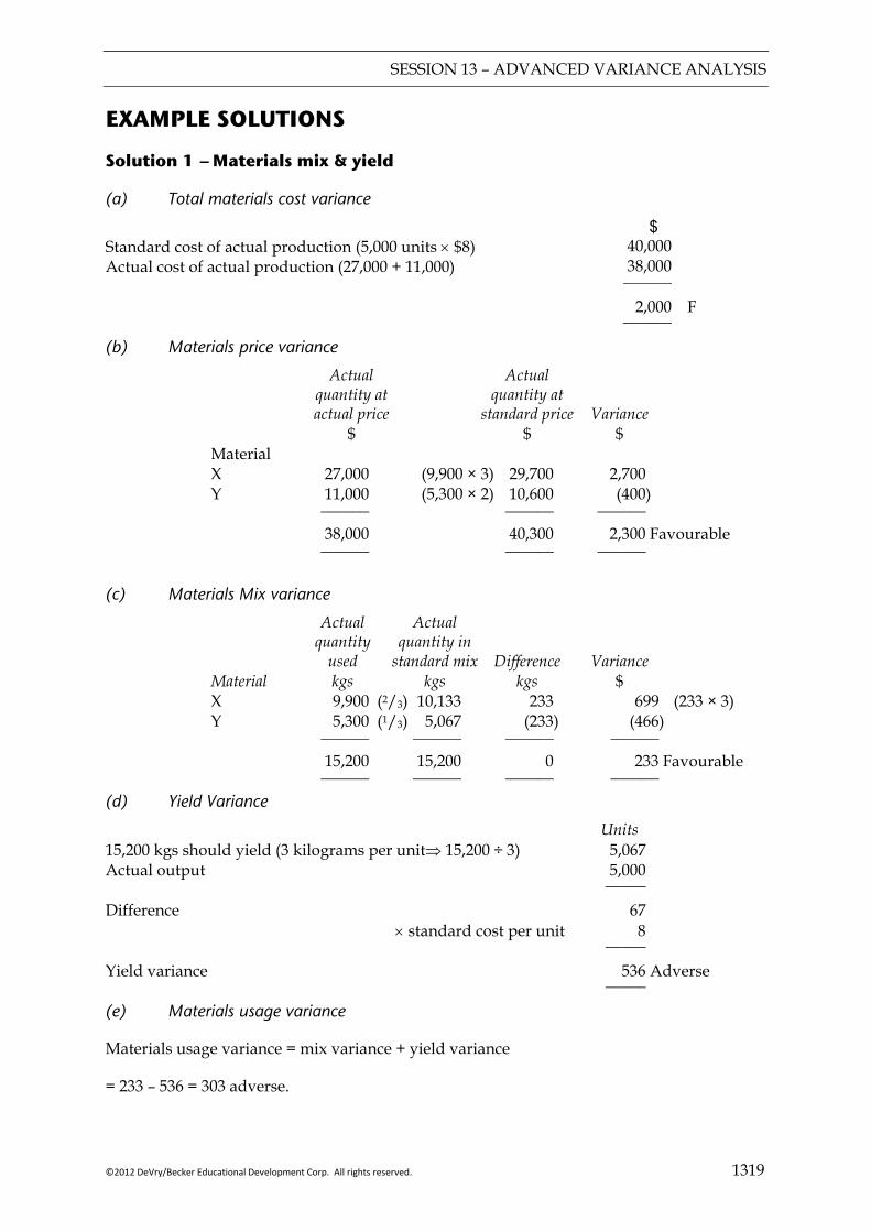
SESSION 13 – ADVANCED VARIANCE ANALYSIS
©2012 DeVry/Becker Educational Development Corp. All rights reserved. 1319
EXAMPLE SOLUTIONS
Solution 1 — Materials mix & yield
(a) Total materials cost variance
$ Standard cost of actual production (5,000 units × $8) Actual cost of actual production (27,000 + 11,000)
40,000 38,000
______ 2,000 ______
F
(b) Materials price variance
Actual Actual quantity at quantity at actual price standard price Variance $ $ $ Material X 27,000 (9,900 × 3) 29,700 2,700 Y 11,000 (5,300 × 2) 10,600 (400) ______ ______ ______
38,000 40,300 2,300 Favourable ______ ______ ______
(c) Materials Mix variance
Actual Actual quantity quantity in used standard mix Difference Variance Material kgs kgs kgs $ X 9,900 (2/3) 10,133 233 699 (233 × 3) Y 5,300 (1/3) 5,067 (233) (466) ______ ______ ______ ______
15,200 15,200 0 233 Favourable ______ ______ ______ ______
(d) Yield Variance
Units 15,200 kgs should yield (3 kilograms per unit⇒ 15,200 ÷ 3) 5,067 Actual output 5,000 _____
Difference 67 × standard cost per unit 8 _____
Yield variance 536 Adverse _____
(e) Materials usage variance
Materials usage variance = mix variance + yield variance
= 233 – 536 = 303 adverse.

SESSION 13 – ADVANCED VARIANCE ANALYSIS
1320 ©2012 DeVry/Becker Educational Development Corp. All rights reserved.
Solution 2 — Sales mix and quantity variances
Price variance $ Q (180*(22 −20)) 360 P (150*(22 −25)) (450) R (170*(26 −30)) (680) _____
(770) _____
Mix variance Actual Sales Actual sales in Standard mix Product sales budgeted Difference margin variance (units) mix (units) (units) $ $ Q 180 250 (70) 3 (210) P 150 125 25 4 100 R 170 125 45 6 270 _____ _____ _____ _____
500 500 0 160 Favourable _____ _____ _____ _____
Commentary The sales mix variance is favourable because customers have switched away from the product Q, which has the lowest margin, and are buying more of products P and R, which have higher margins.
Quantity variance
Actual Sales sales in Budgeted Standard quantity Product budgeted mix sales Difference margin variance (units) (units) (units) $ $ Q 250 200 50 3 150 P 125 100 25 4 100 R 125 100 25 6 150 _____ _____ _____ _____
400 400 Favourable _____ _____ _____ _____

SESSION 13 – ADVANCED VARIANCE ANALYSIS
©2012 DeVry/Becker Educational Development Corp. All rights reserved. 1321
Solution 3 — Activity Based Variances
Calculation of standard costs
= setups of number Budgeted
costs setup Budgeted=
000,3000,800,1 = $ 600 per setup.
Standard output per set up = setups of number Budgeted
output Budgeted=
000,3000,000,30 = 10,000 units
Standard cost per unit = setup per Output
setup per Cost=
000,10600 = $0.06 per unit
Total variance $ 000 24,200,000 units should cost: (24,200,000 × $0.06) 1,452 24,200,000 units did cost 1,550 _____ Total variance 98 (adverse) _____ Overhead expenditure variance $000 Actual overhead cost 1,550 Standard cost for 2,200 setups (2,200 × $600) 1,320 _____
Overhead expenditure variance 230 (adverse)
_____
Efficiency variance
Standard number of set ups for 24,200 units 2,420 Actual number of set ups 2,200 _______ 220 Standard cost per set up $600 _______ Efficiency variance $132,000 (favourable) _______ The overhead expenditure variance + the overhead efficiency variance = -$230,000 + 132,000 = -98,000. This is the total variance.
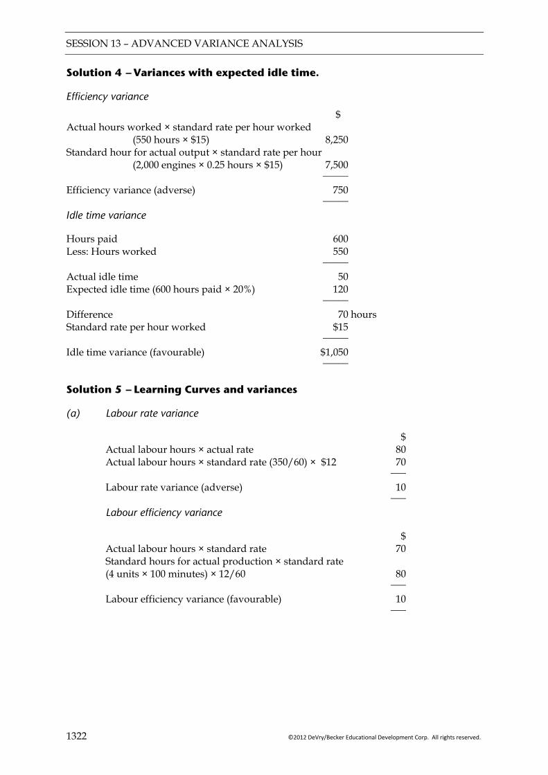
SESSION 13 – ADVANCED VARIANCE ANALYSIS
1322 ©2012 DeVry/Becker Educational Development Corp. All rights reserved.
Solution 4 — Variances with expected idle time.
Efficiency variance
$ Actual hours worked × standard rate per hour worked (550 hours × $15) 8,250 Standard hour for actual output × standard rate per hour (2,000 engines × 0.25 hours × $15) 7,500 _____
Efficiency variance (adverse) 750 _____
Idle time variance
Hours paid 600 Less: Hours worked 550 _____
Actual idle time 50 Expected idle time (600 hours paid × 20%) 120 _____
Difference 70 hours Standard rate per hour worked $15 _____
Idle time variance (favourable) $1,050 _____
Solution 5 — Learning Curves and variances
(a) Labour rate variance
$ Actual labour hours × actual rate 80 Actual labour hours × standard rate (350/60) × $12 70 ___ Labour rate variance (adverse) 10 ___ Labour efficiency variance
$ Actual labour hours × standard rate 70 Standard hours for actual production × standard rate (4 units × 100 minutes) × 12/60 80 ___ Labour efficiency variance (favourable) 10 ___
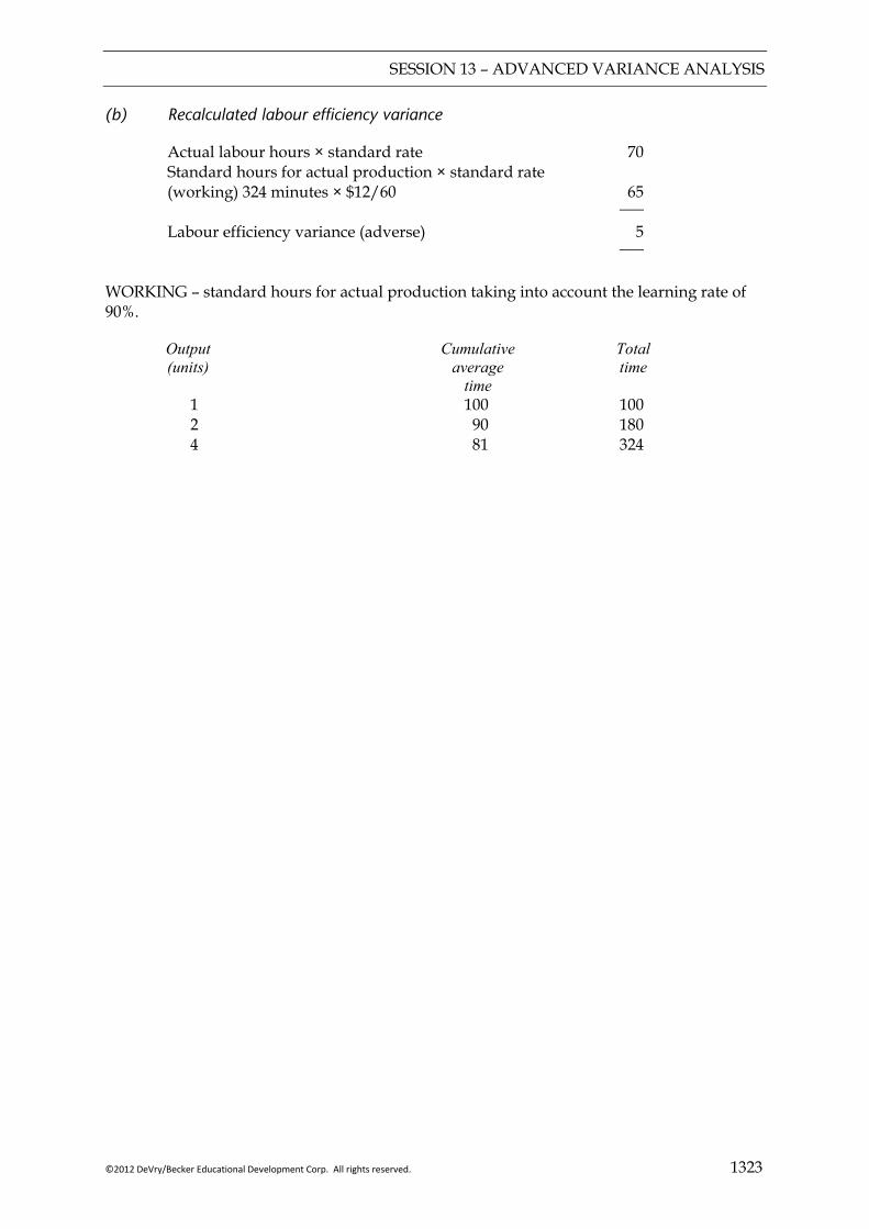
SESSION 13 – ADVANCED VARIANCE ANALYSIS
©2012 DeVry/Becker Educational Development Corp. All rights reserved. 1323
(b) Recalculated labour efficiency variance
Actual labour hours × standard rate 70 Standard hours for actual production × standard rate (working) 324 minutes × $12/60 65 ___ Labour efficiency variance (adverse) 5 ___ WORKING – standard hours for actual production taking into account the learning rate of 90%.
Output Cumulative Total (units) average time time 1 100 100 2 90 180 4 81 324

SESSION 13 – ADVANCED VARIANCE ANALYSIS
1324 ©2012 DeVry/Becker Educational Development Corp. All rights reserved.
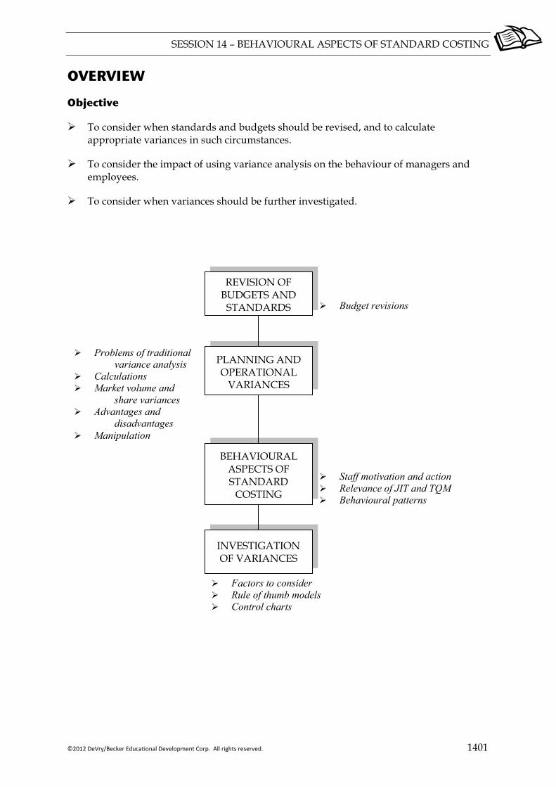
SESSION 14 – BEHAVIOURAL ASPECTS OF STANDARD COSTING
©2012 DeVry/Becker Educational Development Corp. All rights reserved. 1401
OVERVIEW
Objective
To consider when standards and budgets should be revised, and to calculate appropriate variances in such circumstances.
To consider the impact of using variance analysis on the behaviour of managers and employees.
To consider when variances should be further investigated.
REVISION OF BUDGETS AND
STANDARDS Budget revisions
Problems of traditional variance analysis
Calculations Market volume and
share variances Advantages and
disadvantages Manipulation
PLANNING AND OPERATIONAL
VARIANCES
BEHAVIOURAL ASPECTS OF STANDARD
COSTING
INVESTIGATION OF VARIANCES
Staff motivation and action Relevance of JIT and TQM Behavioural patterns
Factors to consider Rule of thumb models Control charts
SESSION 14 − BEHAVIOURAL ASPECTS OF STANDARD COSTING
1402 ©2012 DeVry/Becker Educational Development Corp. All rights reserved.
1 REVISION OF BUDGETS AND STANDARDS
1.1 Budget revisions
At the end of a budget period, prior to comparing the actual performance of an organisation against the budget, budgets may be revised to take account of changes within the environment that were not anticipated when the budget was prepared. The reason for such revision is that since managers are judged on how they performed relative to the budget, it is unfair to use a budget that turns out to be “wrong”.
The principles that should be applied when revising budgets are as follows.
If something occurred during the budget period that was outside of the control of the manager, that meant that the actual budget was not achieved, then the budget should be revised.
If in retrospect, it appears that the original budget was unrealistic for some reason, then the budget may also be revised.
Budgets should not be revised to hide inefficiencies.
Any changes to budgets should be approved by senior management to ensure such revisions are appropriate.
Example 1
The budget for an airline for the year ended 31 December 2011 was prepared in October 2010. Since the budget was prepared, the following events have occurred:
The price of oil has increased by 25% on world markets. This has an impact on the price of fuel for the airline. Fuel accounts for 25% of the airlines costs.
Due to a strike, the airline was not able to operate for four weeks of the year. There was therefore no revenue during this period.
The airline lost an additional two weeks of revenue due to the eruption of the Eyjafjallajokull volcano in Iceland and the associated ash cloud.
Required:
For each of the events above, discuss which should result in the budgets being revised, and which should not.
Solution

SESSION 14 − BEHAVIOURAL ASPECTS OF STANDARD COSTING
©2012 DeVry/Becker Educational Development Corp. All rights reserved. 1403
2 PLANNING AND OPERATIONAL VARIANCES
2.1 Problems of traditional variance analysis
Traditional variance analysis compares:
Actual
performance vs Expected
performance
If the actual environment differs from that which was anticipated when the original standard was set, then management should consider revising the standard (ex-post standard).
Even if the environment has not changed, with hindsight (looking back) it might be realised than an unrealistic standard was used (e.g. ideal standard). Again it might be decided to revise the standard.
The factors to consider in deciding whether to revise a standard are essentially the same as whether to revise a budget. These were discussed in section 1 above.
The variances calculated by comparing actual performance are referred to as operational (or operating) variances. Their calculation is exactly the same as for calculating standard variances, the only difference being that a revised standard has been used.
The difference between the ex-ante and ex-post targets is known as the Planning Variance.
Definitions
Planning variance – a classification of variances caused by ex-ante budget allowances being changed to an ex-post basis.
Operational variance – a classification of variances in which non-standard performance is defined as being that which differs from an ex-post standard.
Commentary Planning variances can relate to any element of the standard product specification. Operational variances are also known as revision variances.
SESSION 14 − BEHAVIOURAL ASPECTS OF STANDARD COSTING
1404 ©2012 DeVry/Becker Educational Development Corp. All rights reserved.
2.2 Calculations
2.2.1 Total cost variances
Use the following table to separate out PLANNING and OPERATING variances.
PLANNING AND OPERATING VARIANCE TABLE
$ ORIGINAL FLEXED BUDGET (EX-ANTE) X REVISED FLEXED BUDGET (EX-POST) X ACTUAL RESULT X
PLANNING VARIANCE (UNCONTROLLABLE)
OPERATING VARIANCE (CONTROLLABLE)
Commentary Planning variances are sometimes referred to as “budget revision variances”. 2.2.2 Planning variances
It is debateable how much useful information planning variances provide to management. However, the total planning variance above can be split into price and usage variances. Various methods may be used. The approach preferred by the examiner is as follows:
Planning usage variance: $ Original SQ × actual output × original SP X Revised SQ × actual output × original SP X __
Planning usage variance X __
Planning price variance $ Revised SQ × actual output × original SP X Revised SQ × actual output × revised SP X __
Planning price variance X __
Where SQ denotes standard quantity per unit and SP denotes standard price per unit.
SESSION 14 − BEHAVIOURAL ASPECTS OF STANDARD COSTING
©2012 DeVry/Becker Educational Development Corp. All rights reserved. 1405
2.2.3 Operating variances
These are calculated in the same way as basic variances. The only change is that the revised standard is used rather than the original standard.
Example 2
Standard material cost/unit : 4 kgs at $2.50 = $10 Budgeted Output : 20,000 units Actual Output : 22,000 units Materials actually used : 86,000 kgs at $3 With hindsight a better standard would have been 3.75 kg per unit at $2.80 per kg.
Required:
(a) Calculate the traditional variances:
(i) Price variance; (ii) Usage variance; (iii) Overall material variance (price + usage).
(b) Calculate the total planning and operating variances.
(c) Analyse the planning variance into price and usage.
(d) Analyse the operating variance into price and usage.
Solution
(a) Traditional price and usage variances
Price variance =
Usage variance =
Total variance = (b) Total planning and operating variances
$ Original flexed budget
Planning variance
Revised flexed budget
Actual result
Operating variance
SESSION 14 − BEHAVIOURAL ASPECTS OF STANDARD COSTING
1406 ©2012 DeVry/Becker Educational Development Corp. All rights reserved.
(c) Planning price and usage variances Planning usage variance
$ Original SQ × actual output × original SP Revised SQ × actual output × original SP ______
Planning usage variance ______
Planning price variance
$ Revised SQ × actual output × original SP Revised SQ × actual output × revised SP ______
Planning price variance ______
(d) Operating price and usage variances
$ Operating price variance
Operating usage variance
Total operating variance
_____
_____
This revised analysis still indicates inefficiency on the part of the buying department and that there could be better use of materials.
Compare this with the traditional analysis that suggested a more serious inefficiency in buying (i.e. $43,000 adverse price variance) coupled with efficient use of materials.
Example 3
Materials budget 3.4kg/unit $2/kg
Actual 2,000 units produced 7,000 kg purchased and used, costing $2.20 per kg.
Required:
(a) Calculate the traditional price and usage variance.
SESSION 14 − BEHAVIOURAL ASPECTS OF STANDARD COSTING
©2012 DeVry/Becker Educational Development Corp. All rights reserved. 1407
Solution
(a) Traditional variances
Traditional price variance =
kg Traditional usage variance
2,000 units should use
Actual usage
Difference
Per kilo
______
= $ ______
Example 3 continued
The purchasing manager is furious when he receives a variance report criticising him. He produces evidence to suggest the average market price during the period was $2.30.
The production manager points out that the usage standard was an ideal standard and totally unrealistic. He calculates the current standard as 3.6kg/unit.
Required:
(b) Calculate:
(i) the total planning and operating variance; (ii) the planning price and usage variance; (iii) the operating price and usage variance.
Solution
(b)(i) total planning and operational variances
$ Original flexed budget
Planning variance
Revised flexed budget
Actual result
Operational variance
SESSION 14 − BEHAVIOURAL ASPECTS OF STANDARD COSTING
1408 ©2012 DeVry/Becker Educational Development Corp. All rights reserved.
(b)(ii) Planning usage and price variances Planning usage variance: $ Original SQ × actual output × original SP Revised SQ × actual output × original SP ______
Planning usage variance ______
Planning price variance $ Revised SQ × actual output × original SP
Revised SQ × actual output × revised SP ______ Planning price variance ______ (b)(iii) Operating price and usage variances $ Operating price variance Kg Operating usage variance 2,000 units should use Actual usage
______ kg @ ______
______
2.3 Market volume and market share variances
2.3.1 The concept
The traditional sales volume variance may have two elements:
The size of the market was different from expected – a change in the external environment;
The share of that market was different from budget.
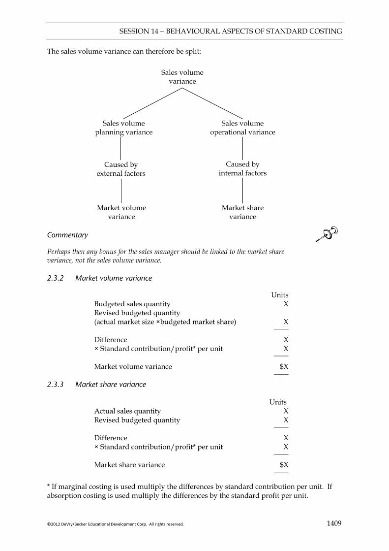
SESSION 14 − BEHAVIOURAL ASPECTS OF STANDARD COSTING
©2012 DeVry/Becker Educational Development Corp. All rights reserved. 1409
The sales volume variance can therefore be split:
Sales volume variance
Sales volume planning variance
Sales volume operational variance
Caused by external factors
Caused by internal factors
Market volume variance
Market share variance
Commentary Perhaps then any bonus for the sales manager should be linked to the market share variance, not the sales volume variance.
2.3.2 Market volume variance
Units Budgeted sales quantity X Revised budgeted quantity (actual market size ×budgeted market share) X ____
Difference X × Standard contribution/profit* per unit X ____ Market volume variance $X ____
2.3.3 Market share variance Units Actual sales quantity X Revised budgeted quantity X ____
Difference X × Standard contribution/profit* per unit X ____ Market share variance $X ____
* If marginal costing is used multiply the differences by standard contribution per unit. If absorption costing is used multiply the differences by the standard profit per unit.
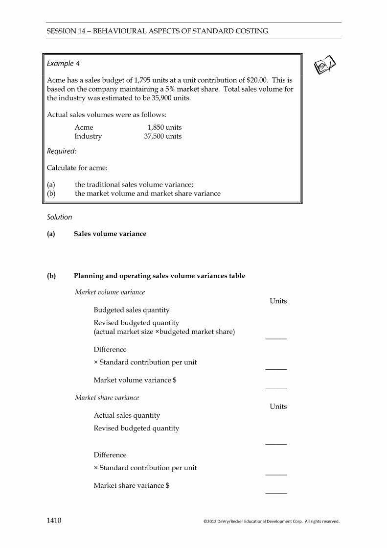
SESSION 14 − BEHAVIOURAL ASPECTS OF STANDARD COSTING
1410 ©2012 DeVry/Becker Educational Development Corp. All rights reserved.
Example 4
Acme has a sales budget of 1,795 units at a unit contribution of $20.00. This is based on the company maintaining a 5% market share. Total sales volume for the industry was estimated to be 35,900 units.
Actual sales volumes were as follows:
Acme 1,850 units Industry 37,500 units Required:
Calculate for acme:
(a) the traditional sales volume variance; (b) the market volume and market share variance
Solution
(a) Sales volume variance
(b) Planning and operating sales volume variances table
Market volume variance Units Budgeted sales quantity
Revised budgeted quantity (actual market size ×budgeted market share) ______
Difference
× Standard contribution per unit ______ Market volume variance $ ______
Market share variance Units Actual sales quantity
Revised budgeted quantity ______
Difference
× Standard contribution per unit ______ Market share variance $ ______
SESSION 14 − BEHAVIOURAL ASPECTS OF STANDARD COSTING
©2012 DeVry/Becker Educational Development Corp. All rights reserved. 1411
2.4 Advantages and disadvantages
2.4.1 Advantages
Distinguishes between variances caused by bad planning or unavoidable factors, and those due to operating factors.
Adverse operating variances indicate processes out of control that need correcting (i.e. feedback control).
Planning variances can be used to update standards to current conditions.
Motivation may improve if managers know they will only be assessed on variances under their control (i.e. operational variances).
2.4.2 Disadvantages
Extra data requirements (e.g. market volume).
More time consuming.
Managers may claim all adverse variances have external causes and all favourable variances internal causes (i.e. manipulation of revised standards).
2.5 Manipulation
From the discussion above, it should be apparent that budgets and standards prepared at the start of the year may need to be revised at the end of the year if they are inappropriate due to factors that occurred outside of the control of the organisation. Care must clearly be taken to ensure that budget revisions are only made when appropriate. Managers who have not achieved their budget targets, or who experience adverse variances may try to hide these by revising the budgets and standards.
In practice therefore, there may be some debate about whether or not a standard or a budget should be revised.
3 BEHAVIOURAL ASPECTS OF STANDARD COSTING
3.1 Effect on staff motivation and action
Standard costing and variance analysis may be used as part of the performance evaluation of managers and staff. As such, variance analysis will have some impact on motivation.
As with budgets, a challenging target can motivate managers and staff to work harder, compared with no target.
SESSION 14 − BEHAVIOURAL ASPECTS OF STANDARD COSTING
1412 ©2012 DeVry/Becker Educational Development Corp. All rights reserved.
However, there are many potential problems of motivation relating to the use of variance analysis:
If variance information is used insensitively, morale may suffer. Employees (the workforce and their supervisors) should be congratulated on tasks well done but management by exception tends to focus on what has gone wrong. If employees are berated or disciplined for adverse variances they may attempt to cover them up or take actions to ensure that the variances within their control are favourable, which may not be in the best interests of the firm. For example, in rushing to increase productivity at the end of the budget period to avoid an unfavourable labour efficiency variance the quality of output may suffer.
Accurate preparation of standards can be difficult (e.g. during trial runs workers may operate below their ability to build “slack” into the standard).
Labour quantity standards and efficiency variances make two assumptions that may not hold true:
(1) If workers works faster, output will go up (i.e. the pace of production is dictated by labour). However, the volume of output may be influenced more by the processing speed of equipment.
(2) That labour is a variable cost. However, the cost of a workforce may be essentially fixed. Undue emphasis on efficiency can results in an excessive build-up of work in process and finished goods inventories.
3.2 Relevance in the modern environment of JIT and TQM
Many writers have argued that variance analysis is not relevant in the modern business world, and can lead to dysfunctional behaviour for the following reasons:
Use of standard costing system may lead to over-emphasis on quantitative elements of performance. It is important that qualitative performance is not neglected (e.g. customer satisfaction, employee morale, and innovation) particularly in a total quality management environment.
Just in time (JIT) systems and flexible manufacturing systems aim to provide more tailored production to meet customers’ needs. There may therefore be less standardisation of production which makes comparison with a standard less meaningful.
In JIT purchasing systems there is emphasis on forging close, long-term relations with suppliers. Under such a system, it is likely that input costs will be known with certainty in advance, so there will be no price variances.
Traditional standard setting is based on a company’s own costs and procedures. This may be too inward looking where the company operates in a rapidly changing, competitive market.
A more modern approach is benchmarking which also takes into account the practices of other organisations in the industry (i.e. external information).

SESSION 14 − BEHAVIOURAL ASPECTS OF STANDARD COSTING
©2012 DeVry/Becker Educational Development Corp. All rights reserved. 1413
3.3 Behavioural patterns in rapidly changing environments
The use of standard costing and variance analysis can have adverse impacts on behaviour in a rapidly changing environment.
Merely meeting standards may be insufficient to ensure survival of a firm in a competitive environment. Thus it may be necessary to focus on trends in variances that aim for continual improvement.
Standards provide an internal focus to management. In a rapidly changing environment, an external focus would be more appropriate.
New products come on line more frequently. There may be learning curves associated with these. If these are not reflected in standards, standards may not be set at an appropriate level. They could be too easy, which would not challenge staff, or too difficult, which would demotivate.
4 INVESTIGATION OF VARIANCES
4.1 Factors to consider
Variance analysis is a control tool. The cause of a variance may be investigated and appropriate action taken to ensure that the variance does not occur in future. This is aimed at making it more likely that the company will meet their budgets.
There are therefore many factors to consider when deciding whether or not to investigate variances:
4.1.1 Size
Larger cost savings are likely to arise from taking action to correct large variances and a policy could be established of investigating all variances above a given size.
4.1.2 Adverse or favourable
It is natural to concentrate on adverse variances in order to bring business operations back in line with budget. However, whether a variance is adverse or favourable should not influence the decision to investigate. The reasons for favourable variances should also be sought as they may indicate the presence of budgetary slack or suggest ways in which the budgeting process could be improved. Favourable variances may also indicate areas where the budget is easy to achieve, suggesting that the motivational effect of a budget could be improved by introducing more demanding targets.
4.1.3 Cost versus benefits
If the expected cost of investigating a variance is likely to exceed any benefits expected to arise from its correction, it may be decided not to investigate.
4.1.4 Historic pattern of variances
A variance that is unusual when compared to historic patterns of variances may be considered worthy of investigation. Statistical tests of significance may be used to highlight such variances.
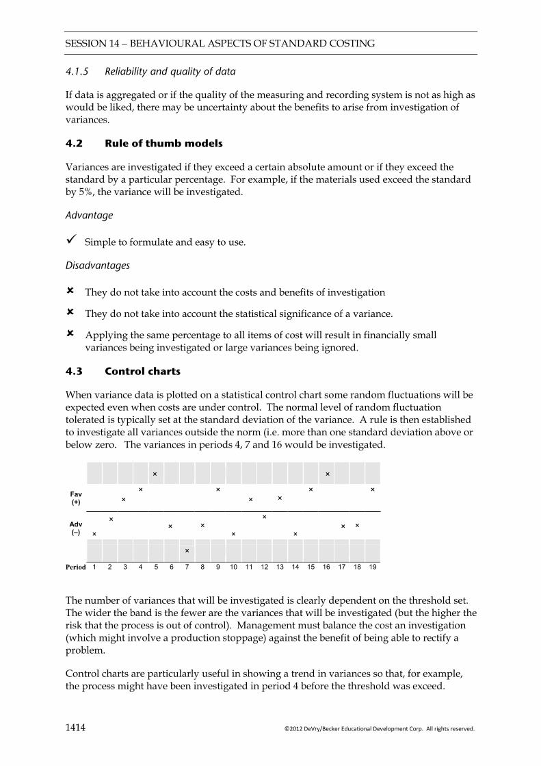
SESSION 14 − BEHAVIOURAL ASPECTS OF STANDARD COSTING
1414 ©2012 DeVry/Becker Educational Development Corp. All rights reserved.
4.1.5 Reliability and quality of data
If data is aggregated or if the quality of the measuring and recording system is not as high as would be liked, there may be uncertainty about the benefits to arise from investigation of variances.
4.2 Rule of thumb models
Variances are investigated if they exceed a certain absolute amount or if they exceed the standard by a particular percentage. For example, if the materials used exceed the standard by 5%, the variance will be investigated.
Advantage
Simple to formulate and easy to use.
Disadvantages
They do not take into account the costs and benefits of investigation
They do not take into account the statistical significance of a variance.
Applying the same percentage to all items of cost will result in financially small variances being investigated or large variances being ignored.
4.3 Control charts
When variance data is plotted on a statistical control chart some random fluctuations will be expected even when costs are under control. The normal level of random fluctuation tolerated is typically set at the standard deviation of the variance. A rule is then established to investigate all variances outside the norm (i.e. more than one standard deviation above or below zero. The variances in periods 4, 7 and 16 would be investigated.
× ×
Fav (+) ×
×
× × ×
×
×
Adv (–) ×
× × × ×
×
×
× ×
× Period 1 2 3 4 5 6 7 8 9 10 11 12 13 14 15 16 17 18 19
The number of variances that will be investigated is clearly dependent on the threshold set. The wider the band is the fewer are the variances that will be investigated (but the higher the risk that the process is out of control). Management must balance the cost an investigation (which might involve a production stoppage) against the benefit of being able to rectify a problem.
Control charts are particularly useful in showing a trend in variances so that, for example, the process might have been investigated in period 4 before the threshold was exceed.
SESSION 14 − BEHAVIOURAL ASPECTS OF STANDARD COSTING
©2012 DeVry/Becker Educational Development Corp. All rights reserved. 1415
Key points
Actual performance is compared with budgets at the end of each budget period. Prior to performing this comparison, it may be appropriate to revise the budget if it turns out to be unrealistic in retrospect, or if factors outside the control of the relevant manager occurred which made the original budget inappropriate.
Standards may also be revised prior to performing variance analysis. “Operational variances” is a term used to describe variances calculated by comparing actual performance against a revised standard.
Planning variances may also be performed to calculate the effect of changing the standard. For materials, two variances are calculated:
planning usage variance: (Original SQ × actual output × original SP) – (Revised SQ × actual output × original SP)
planning price variance: (Revised SQ × actual output × original SP) – (Revised SQ × actual output × revised SP)
The sales volume variance can also be analysed into a market volume (planning) variance and a market share (operational) variance. A revised budgeted sales quantity is found by multiplying the budgeted market share with the actual market size.
Market volume variance is then (Original budget quantity – Revised standard quantity) × standard contribution per unit.
Market volume variance is (Revised standard quantity – actual sales quantity) × standard contribution per unit.
The use of standard costing and variance analysis is aimed at improving the efficiency of operations. Managers need to be aware of the potential adverse effects that variance analysis can have on the behaviour of those that are being appraised.
SESSION 14 − BEHAVIOURAL ASPECTS OF STANDARD COSTING
1416 ©2012 DeVry/Becker Educational Development Corp. All rights reserved.
FOCUS
You should now be able to:
calculate a revised budget;
identify and explain those factors which that could and could not be allowed to revise an original budget;
calculate planning and operational variances for sales, including market size and market share materials and labour;
explain the manipulation issues in revising budgets;
describe the dysfunctional nature of some variances in the modern environment of JIT and TQM;
discuss the behavioural problems resulting from using standard costs in rapidly changing environments;
discuss the effect that variances have on staff motivation and action;
explain the different methods available for deciding whether or not to investigate a variance.
SESSION 14 − BEHAVIOURAL ASPECTS OF STANDARD COSTING
©2012 DeVry/Becker Educational Development Corp. All rights reserved. 1417
EXAMPLE SOLUTIONS
Solution 1 — Budget revisions
Budget revisions should be made in the case of the increase in fuel costs and the volcano ash- as these are clearly outside of the control of the management.
The lost revenue from the strike is less clear. On the one hand, the strike could be “blamed” on the management, for poor industrial relations. It would therefore be inappropriate to revise the budget for this, and management should be “blamed” for the loss of revenue during this period. On the other hand it could be argued that since the unions called the strike, it was outside of the control of management.
Commentary While the answer above may appear a little “woolly” in that it does not reach a definite conclusion, it is worth realising that in the real world, there are often situations where there is no “right” answer. In F5 exams, the examiner wants “both sides of the argument” rather than a quick conclusion, for questions of this nature.
Solution 2 — Materials
(a) Traditional price and usage variances
Price variance (2.50 – 3.00) 86,000 = $43,000 Adverse
Usage variance (22,000 × 4 – 86,000) $2.50 = $5,000 Favourable
Total variance = $38,000 Adverse (b) Total planning and operating variances
$ Original flexed budget
22,000 × 4 × $2.50
220,000
Planning variance $11,000 Adverse
Revised flexed budget 22,000 × 3.75 × $2.8
231,000
Actual result
86,000 kg × $3
258,000
Operating variance
$27,000 Adverse
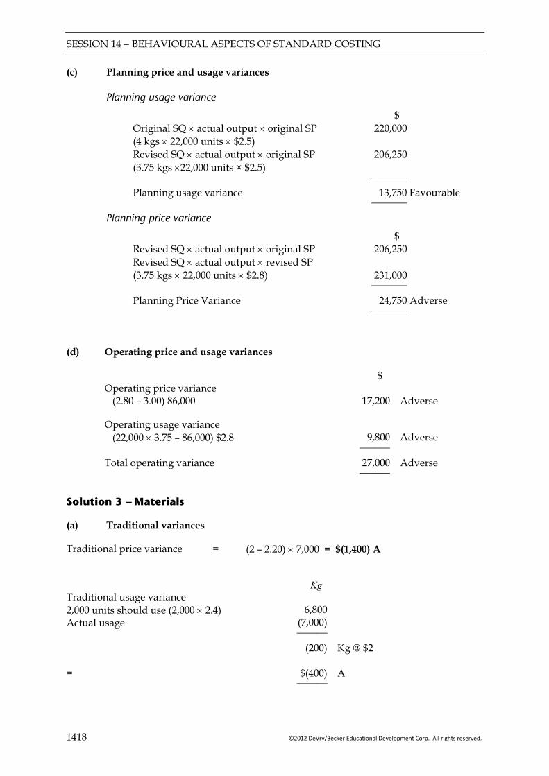
SESSION 14 − BEHAVIOURAL ASPECTS OF STANDARD COSTING
1418 ©2012 DeVry/Becker Educational Development Corp. All rights reserved.
(c) Planning price and usage variances Planning usage variance
$ Original SQ × actual output × original SP 220,000 (4 kgs × 22,000 units × $2.5) Revised SQ × actual output × original SP 206,250 (3.75 kgs ×22,000 units × $2.5) _______
Planning usage variance 13,750 Favourable _______
Planning price variance
$ Revised SQ × actual output × original SP 206,250 Revised SQ × actual output × revised SP (3.75 kgs × 22,000 units × $2.8) 231,000 _______
Planning Price Variance 24,750 Adverse _______
(d) Operating price and usage variances
$ Operating price variance
(2.80 – 3.00) 86,000
17,200 Adverse
Operating usage variance (22,000 × 3.75 – 86,000) $2.8
9,800
Adverse
Total operating variance
______ 27,000 ______
Adverse
Solution 3 — Materials
(a) Traditional variances
Traditional price variance = (2 – 2.20) × 7,000 = $(1,400) A
Kg Traditional usage variance 2,000 units should use (2,000 × 2.4) Actual usage
6,800
(7,000)
______ (200)
Kg @ $2
= $(400) ______
A

SESSION 14 − BEHAVIOURAL ASPECTS OF STANDARD COSTING
©2012 DeVry/Becker Educational Development Corp. All rights reserved. 1419
(b)(i) Total planning and operational variances
$ Original flexed budget
2,000 × 3.4kg × $2
13,600
Planning variance (2,960)
Revised flexed budget 2,000 × 3.6 kg × $2.30
16,560
Actual result
(7,000 × 2.20)
15,400
Operational variance 1,160 F
(b)(ii) Planning usage and price variances Planning usage variance
$ Original SQ × actual output × original SP 13,600 (3.4kg × 2,000 units × $2) Revised SQ × actual output × original SP (3.6kg × 2,000 units × $2) 14,400 ______
Planning usage variance 800 Adverse ______
Planning price variance
$ Revised SQ × actual output × original SP 14,400 Revised SQ × actual output × revised SP (3.6kg × 2,000 units × $2.3) 16,560 ______
Planning price variance 2,160 Adverse ______
(b)(iii) Operating price and usage variances
Operating price variance = (2.30 – 2.20) × 7,000 = 700F
Kg Operating usage variance 2,000 units should use (2,000 × 3.6) Actual usage
7,200
(7,000)
______ 200 Kg @ 2.30 $460 F ______
$1,160 ______
F
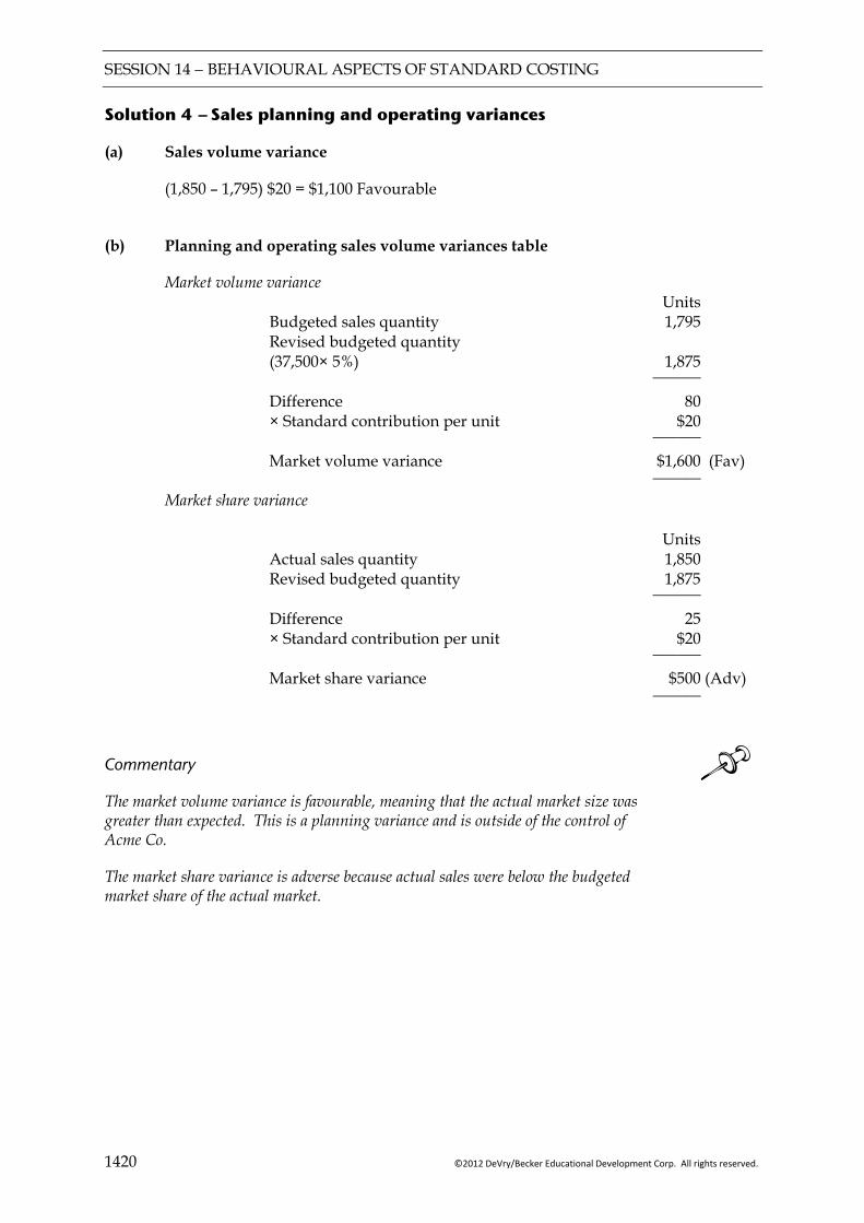
SESSION 14 − BEHAVIOURAL ASPECTS OF STANDARD COSTING
1420 ©2012 DeVry/Becker Educational Development Corp. All rights reserved.
Solution 4 — Sales planning and operating variances
(a) Sales volume variance
(1,850 – 1,795) $20 = $1,100 Favourable
(b) Planning and operating sales volume variances table
Market volume variance Units Budgeted sales quantity 1,795 Revised budgeted quantity (37,500× 5%) 1,875 ______
Difference 80 × Standard contribution per unit $20 ______ Market volume variance $1,600 (Fav) ______
Market share variance Units Actual sales quantity 1,850 Revised budgeted quantity 1,875 ______
Difference 25 × Standard contribution per unit $20 ______ Market share variance $500 (Adv) ______
Commentary The market volume variance is favourable, meaning that the actual market size was greater than expected. This is a planning variance and is outside of the control of Acme Co.
The market share variance is adverse because actual sales were below the budgeted market share of the actual market.
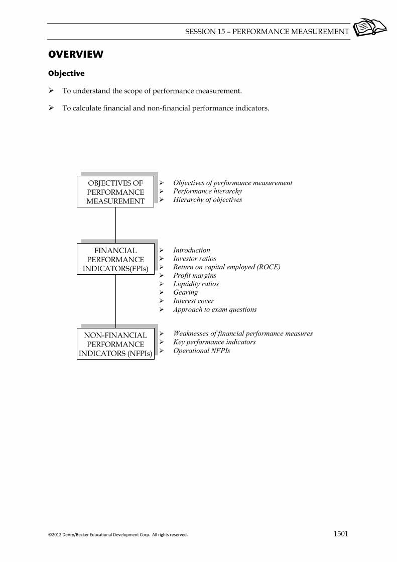
SESSION 15 – PERFORMANCE MEASUREMENT
©2012 DeVry/Becker Educational Development Corp. All rights reserved. 1501
OVERVIEW
Objective
To understand the scope of performance measurement.
To calculate financial and non-financial performance indicators.
OBJECTIVES OF PERFORMANCE MEASUREMENT
FINANCIAL PERFORMANCE
INDICATORS(FPIs)
NON-FINANCIAL PERFORMANCE
INDICATORS (NFPIs)
Introduction Investor ratios Return on capital employed (ROCE) Profit margins Liquidity ratios Gearing Interest cover Approach to exam questions
Objectives of performance measurement Performance hierarchy Hierarchy of objectives
Weaknesses of financial performance measures Key performance indicators Operational NFPIs
SESSION 15 – PERFORMANCE MEASUREMENT
1502 ©2012 DeVry/Becker Educational Development Corp. All rights reserved.
1 OBJECTIVES OF PERFORMANCE MEASUREMENT
1.1 Objectives of performance measurement
As part of the corporate strategy planning of an organisation, the directors will define the objectives of the organisation. These objectives may be organised into a hierarchy of objectives, the performance hierarchy.
Performance measurement aims to measure how successfully the organisation is achieving its objectives. As such, they from part of the control system of an organisation.
The main objectives of a system of performance measurement are:
Designing measures at all levels of an organisation which are consistent with the strategy of the organisation.
Setting targets based on those measures.
Reward schemes should be based on performance of managers against the targets
Measures should be fair; managers should only be judged on things they control.
Measures should be objective and quantifiable; not subjective.
1.2 The performance hierarchy
The idea of the performance hierarchy was introduced in the session on budgeting. As a reminder, the objectives of an organisation are often based on a hierarchy – the performance hierarchy. Typically the hierarchy consists of:
Mission – the main reason for the existence of the organisation.
Corporate Objectives – more concrete objectives, stating what the mission means in practical terms to the primary stakeholder groups (e.g. to increase the market value of the company by more than a given percentage, over the longer term).
Subsidiary Objectives – other objectives of the organisation may relate to other stakeholder groups (e.g. to reduce the amount of pollution by a given percentage).
Unit Objectives – these are objectives for the operating departments (units) of the organisation. They should contribute to the subsidiary and corporate objectives.
1.3 Hierarchy of objectives
Since there is a hierarchy of objectives, there will also be a hierarchy of performance measures. Performance targets and measures will be set at all levels within the organisation. In a well-designed system, these targets and measures will be consistent with the organisations overall goals.
SESSION 15 – PERFORMANCE MEASUREMENT
©2012 DeVry/Becker Educational Development Corp. All rights reserved. 1503
2 FINANCIAL PERFORMANCE INDICATORS (FPIs)
2.1 Introduction
Traditional performance measurement was based solely on financial measures. This was considered to be appropriate, because it was assumed that the primary objective of all organisations was to maximise the wealth of their shareholders. It seemed natural therefore that focusing on financial measures would help to achieve this objective.
Much of the material covered already in earlier sessions of this Study System relates to FPIs, in particular:
Budgeting; Standard costing and variances; Activity based costing; Specialist management accounting techniques.
This section introduces some additional, widely used ratios that are also used for financial performance evaluation.
2.2 Return on equity and return on capital employed (ROCE)
Return on equity = 100Equity
tax after Profit×
Return on capital employed = 100 sliabilitie term-long + reserves + Shares
tax and interest BEFORE Profit×
Commentary In practice, variants of the above formulae may be used. What is important is to match the profit figure with the appropriate capital. If profit is expressed after interest, then it should be divided by equity. If profit is expressed before interest, then it should be divided by equity plus long term debt, since profit before interest will be shared among providers of debt and equity finance.
2.2.1 Meaning of return on capital employed
Shows the return generated on the company’s profit. This can be compared to other companies in the same industry sector, or to the company’s cost of capital.
Comparing companies in other sectors does not provide valid information. Service industries, for example, tend to have higher return on capital due to the fact that less capital is required than for manufacturing industries.
2.2.2 Methods to improve return on capital employed ratios
Invest in projects that generate a higher return on capital
Manipulate profits and capital employed by using different accounting policies.

SESSION 15 – PERFORMANCE MEASUREMENT
1504 ©2012 DeVry/Becker Educational Development Corp. All rights reserved.
Delay investment in new plant and machinery or reduce investment on intangible assets. As the non-current assets become depreciated, their carrying amount (net book value) falls, reducing the capital employed, and therefore improving the return on capital. Such measures may harm the organisation in the longer term.
2.3 Profit margins
Profit margins relate profit to revenue. Since there are many profit sub totals in the income statement (Gross Profit, Profit before interest and tax etc. ) there are many potential profit margins. The most commonly used are the gross profit margin and the net profit margin.
2.3.1 Gross profit margin
100Revenue
profit Gross×
2.3.2 Meaning of gross profit margin
Gross profit means profit after deducting the costs of buying or making the products that the company produces. It therefore reflects the performance of the company’s products.
A fall in gross profit margin over time means that either the selling price at which the company sells its goods is declining, or that the cost of making or buying those goods is increasing, but those increases cannot be passed onto customers. In either case, a prolonged decline is a bad sign. It suggests that the products or services that the company sells are losing popularity, and this puts into question the viability of the business.
Gross profit margins may also reflect an organisation’s pricing strategy. Companies that use a premium pricing strategy are likely to have a high gross profit margin. Companies that aim to sell for a low price, but to achieve a larger volume of sales, are likely to have a low gross profit margin.
2.3.3 Methods to improve gross profit margins
Introduce new products which are popular with customers. These can be sold for a higher margin.
Use target costing to reduce cost of sales.
Gross profit depends on the company’s policy regarding what is considered as a direct expense and what is an administrative expense. Changes in such policies should be viewed with suspicion.
2.3.4 Net profit margin
100Revenue
tax after Profit×
SESSION 15 – PERFORMANCE MEASUREMENT
©2012 DeVry/Becker Educational Development Corp. All rights reserved. 1505
2.3.5 Meaning of net profit margin
Net profit is sometimes referred to as “the bottom line” as it is profit after deducting all costs. The net profit margin shows overall profits as a percentage of revenue. While this gives a broad indicator of the performance of the organisation, further analysis of the causes of changes will need to be investigated. Net profit margin reflects the following three areas:
The underlying popularity of the company’s products and services (this is also reflected in the gross margin).
The amount of control the company has over administrative type expenses.
Costs of debt financing. This will depend partly on whether the company has changed the amount of debt, and partly on whether interest rates have changed.
2.3.6 Ways to improve the net profit margin
The net profit margin can be improved by the following methods:
Introduce new products which are popular with customers. These can be sold for a higher margin.
Use target costing to reduce cost of sales.
Increase sales volume should increase net profit margins if a high portion of the company’s costs are fixed (e.g. in a training company).
Better control over administrative expenses (e.g. salaries).
Using less debt finance.
2.4 Liquidity ratios
Liquidity ratios measure the ability of the organisation to meet its liabilities as they become due. In particular, the ability to repay suppliers, interest on bank loans, and to repay bank loans and overdrafts when they become due. If a company is not able to do this, the people that the company owes money to could take legal action which in the worst case could lead to the company being liquidated. Many profitable companies face liquidity problems.
The ultimate measure of liquidity is the company’s operating cash flows. If the company generates positive operating cash flows on an on-going basis, and these are more than sufficient to replace any non-current assets, then the company is less likely to experience liquidity problems.
2.4.1 Current ratio
end) period (at sliabilitie Currentend) period (at assets Current

SESSION 15 – PERFORMANCE MEASUREMENT
1506 ©2012 DeVry/Becker Educational Development Corp. All rights reserved.
2.4.2 Quick Ratio (acid test ratio
end) period (at sliabilitie Currentend) period (at inventory assets Current −
2.4.3 Meaning of current and quick ratios
The current ratio is simply a measure of whether or not the organisation’s current assets exceed its current liabilities. If the ratio is less than 1, then current liabilities exceed the current assets.
The quick ratio is a more conservative version of the current ratio. Some analysts argue that inventory is not a liquid asset, so should not be considered to be a current asset. It is sometimes referred to as the “acid test”.
Commentary Literally, an acid test is a test to determine whether a metal is real gold or not. A low or declining ratio may indicate that the company is starting to experience problems in meeting its liabilities. This could be due to not generating sufficient profits and cash flows, so that the company cannot afford to pay its suppliers on time. It could also be due to large investment in non-current assets.
Commentary The fact that there is no value for the current ratio that indicates satisfactory liquidity can be illustrated by one major international food retailer, which regularly reports a current ratio of around 0.3. The company in question has low inventory as food only lasts a few days. It has few receivables, as most of its sales are for cash. Cash balances are invested in non-current assets, so low cash balances are held. The company does not pay its suppliers for three months, so it has large payables balances. Far from indicating that this company has liquidity problems, the company is using its suppliers as a free source of financing for the business.
2.4.4 Ways to increase liquidity ratios
Use long term finance, loans and equity, to finance the acquisition of non-current assets.
Generate positive cash flows so that short term liabilities can be repaid on time.
Can be manipulated by window dressing at the year end:

SESSION 15 – PERFORMANCE MEASUREMENT
©2012 DeVry/Becker Educational Development Corp. All rights reserved. 1507
Example 1
Extracts from the Statement of financial position
$000
Receivables 900 Cash 500 Payables 1,000
Required:
(a) Calculate the quick ratio.
(b) Recalculate the ratio if $400,000 of payments are made just prior to the year end.
Solution
(a) Quick ratio =
(b) Quick ratio =
Commentary Current ratio and quick ratio can be manipulated as demonstrated in Example 1 above, where a payment is made just prior to the year end in order to improve the reported liquidity position at the end of the year.
2.5 Gearing
Gearing (or “leverage”) measures what portion of a company’s finance is provided by debt. The advantage of debt is that it is a cheap source of financing. Providers of debt require a lower return than providers of equity finance as they face less risk. Interest on debt is also a tax deductible expense, which further reduces to cost of debt.
On the other hand, if companies have too much debt, (gearing) they increase the risk of not being able to repay the interest on the debt.
Two gearing ratios are commonly used:
EquityDebt × 100 (gives gearing as a percentage)
Or debt plus Equity
Debt x 100

SESSION 15 – PERFORMANCE MEASUREMENT
1508 ©2012 DeVry/Becker Educational Development Corp. All rights reserved.
Commentary Measures the proportion of borrowed funds (which earn a fixed return) to equity capital (shareholders’ funds) and provide information about the financial risk of a company.
Illustration 1
A B C $ $ $
Shares and accumulated profit 10,000 3,000 7,500 Long term debt – 7,000 2,500 ______ ______ ______
Capital employed 10,000 10,000 10,000 ______ ______ ______
Solution
No gearing 70% 25% highly low geared gearing
2.5.1 Meaning of gearing
A gearing ratio in isolation means very little. It is only useful if the gearing of the organisation is compared to industry averages, or to other companies in the same business area to determine whether the gearing is too high or not.
In industries with stable profits, companies can sustain higher levels of gearing. In companies where profits fluctuate, a high level of gearing is more dangerous, since a fall in profits may mean the company is unable to repay interest on its loans.
An increase in the gearing of one company over time may reflect a change in policy of the finance director relating to the amount of debt that is seen as acceptable. Alternatively it may indicate that the company is not generating sufficient cash flows and is borrowing money to support short term operations.
2.6 Interest cover
Interesttax) (and interest before Profit
2.6.1 Meaning of interest cover
To show the extent to which return on debt (interest) is covered by profit. (Before tax because interest is an allowable expense for income tax purposes.)
Used by lenders to determine vulnerability of interest payments to a drop in profit.

SESSION 15 – PERFORMANCE MEASUREMENT
©2012 DeVry/Becker Educational Development Corp. All rights reserved. 1509
2.7 Approach to financial performance evaluation exam questions
2.7.1 Comments not calculations
In paper F5, the examiner does not give many marks for simply calculating ratios in performance evaluation questions. She is looking for candidates to show that they have the ability to comment on what the numbers and calculations show about how the organisation has performed.
2.7.2 Approach
Before writing anything, spend a few minutes reviewing the information and analysing it. The following is a suggested approach to this planning time:
Review the “big picture” – look at revenue growth, profit growth, and any other major trends that you can see from the data.
Calculate a limited number of ratios that you think are necessary to investigate further any trends identified in the analysis above (e.g. if revenues have grown, but profits have not changed, it may be worth calculating gross profit margins to identify if this is the cause of the sluggish profits).
If capital is given, calculate return on capital employed as this can be an important indicator of how the organisation is providing a return on the capital invested.
Review the information given in the scenario and look for clues that might explain the trends. Information such as “the company operates in a competitive environment” might explain falling gross profit margins.
Having planned in this way, start to write your answer. Comment on each trend identified.
Comment means:
Say what has happened (e.g. profits increased by 20% between quarter 1 and quarter 2).
Say why this has happened. Use any relevant information provided in the scenario to help identify why (e.g. revenue increased by 10% and many of the company’s costs are fixed, so this has led to a 20% rise in profits.)
Link this to other related items. For example, if depreciation rose significantly due to investment in new machinery, perhaps spending on repairs may have fallen.
Express an opinion (e.g. an increase of profits of 20% is impressive given that the company is operating in a competitive environment.)
It is a good idea to show any ratio calculations separately (e.g. in an appendix). This looks professional.
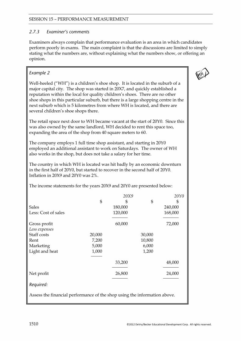
SESSION 15 – PERFORMANCE MEASUREMENT
1510 ©2012 DeVry/Becker Educational Development Corp. All rights reserved.
2.7.3 Examiner’s comments
Examiners always complain that performance evaluation is an area in which candidates perform poorly in exams. The main complaint is that the discussions are limited to simply stating what the numbers are, without explaining what the numbers show, or offering an opinion.
Example 2
Well-heeled (“WH”) is a children’s shoe shop. It is located in the suburb of a major capital city. The shop was started in 20X7, and quickly established a reputation within the local for quality children’s shoes. There are no other shoe shops in this particular suburb, but there is a large shopping centre in the next suburb which is 5 kilometres from where WH is located, and there are several children’s shoe shops there.
The retail space next door to WH became vacant at the start of 20Y0. Since this was also owned by the same landlord, WH decided to rent this space too, expanding the area of the shop from 40 square meters to 60.
The company employs 1 full time shop assistant, and starting in 20Y0 employed an additional assistant to work on Saturdays. The owner of WH also works in the shop, but does not take a salary for her time.
The country in which WH is located was hit badly by an economic downturn in the first half of 20Y0, but started to recover in the second half of 20Y0. Inflation in 20X9 and 20Y0 was 2%.
The income statements for the years 20X9 and 20Y0 are presented below:
20X9 20Y0 $ $ $ $ Sales 180,000 240,000 Less: Cost of sales 120,000 168,000 _______ _______
Gross profit 60,000 72,000 Less expenses Staff costs 20,000 30,000 Rent 7,200 10,800 Marketing 5,000 6,000 Light and heat 1,000 1,200 _____
33,200 48,000 _______ _______
Net profit 26,800 24,000 _______ _______
Required:
Assess the financial performance of the shop using the information above.
SESSION 15 – PERFORMANCE MEASUREMENT
©2012 DeVry/Becker Educational Development Corp. All rights reserved. 1511
3 NON-FINANCIAL PERFORMANCE INDICATORS (NFPIs)
3.1 Weaknesses of financial performance measures
Traditional performance measurement was based almost exclusively on financial measures. However, since the 1980s, many companies recognised that there are inherent weaknesses in focusing only on financial factors:
They lead to excessive focus on cost reduction. Short-term cost reductions may be achieved at the expense of long-term performance due to the effect on staff morale, quality, and other factors.
FPIs ignore the drivers of business success. The things which drive business success are:
Quality Delivery Customer satisfaction After sales service
The examiner for paper F5 believes that organisations are obsessed with financial measures of performance, whereas NFPIs drive businesses forward in the long run. FPIs may measure success, but they do not ensure success.
Since the 1980s therefore, many companies have started to develop non-financial performance indicators.
Since companies have a hierarchy of objectives, they also have a hierarchy of performance measures.
3.2 Key performance indicators
At the strategic level, many companies identify their critical success factors.
Definition
A critical success factor is something the organisation must do to meet its mission.
Organisations should only identify a small number of critical success factors.
Key performance indicators are measures of how well the organisation is meeting its critical success factors.
SESSION 15 – PERFORMANCE MEASUREMENT
1512 ©2012 DeVry/Becker Educational Development Corp. All rights reserved.
Illustration 3
Vodafone Group plc, the British multi-national mobile telephone operator monitors the following Key performance indicators on a quarterly basis:
Vodafone live! active devices and 3G devices; Active customers; Average monthly revenue per user (ARPU); Non-voice services as a percentage of service revenues; Customer churn; Voice usage volumes.
3.3 Operational NFPIs
Having set NFPIs at the strategic level, non-financial performance measures can be set be set at all levels of an organisation. Measures chosen should be consistent with the organisations overall goals.
Example 3
Required:
Suggest some possible non-financial performance measures that might be used in a manufacturing organisation to measure the following attributes:
Product quality; Product delivery; Customer satisfaction; After sales service.
Advantages of NFPIs
They are usually easier to calculate than financial reports, so can be provided much more quickly (e.g. at the end of each shift).
They are more flexible as organisations can come up with any measures that are appropriate to their objectives.
NFPIs are less easily manipulated than financial measures.
SESSION 15 – PERFORMANCE MEASUREMENT
©2012 DeVry/Becker Educational Development Corp. All rights reserved. 1513
3.4 Ways to improve performance indicated by non-financial indicators
3.4.1 Quality indicators
Many organisations use quality improvement programmes to improve the measured quality of products or services. Such programmes normally include quality control and quality assurance:
Quality control focuses on measuring the quality of the products and comparing this against a pre-determined standard. Typically this involves the use of quality inspectors.
Quality assurance means having procedures in place to ensure good quality. This might include redesigning processes, using better quality materials, and the use of “quality meetings” during which staff are asked to make suggestions as to how quality can be improved.
3.4.2 Customer service
Customer service is particularly important in services industries, but also in manufacturing industries the level of after sales service is important.
Ways to improve performance indicated include
Provide training to staff so they understand the importance of customer service.
Providing incentives to staff (e.g. “employee of the month” rewards and prizes for good performance) may lead to improvements in this area.
3.5 Target setting in qualitative areas
The session on budgeting and standard costing dealt with problems inherent in setting financial targets. Most of the issues relating to setting financial targets also apply to qualitative areas too. However, in qualitative areas, there may be additional complications.
3.5.1 Qualitative areas of performance
When looking at qualitative (non-financial) areas, the most important areas of performance tend to be:
Quality of product or service; Customer satisfaction; Delivery; After sales service.
These are the areas that organisations wish to measure using NFPIs.
SESSION 15 – PERFORMANCE MEASUREMENT
1514 ©2012 DeVry/Becker Educational Development Corp. All rights reserved.
3.5.2 Difficulties of setting targets for qualitative areas
When setting targets for qualitative areas, the following difficulties will be experienced:
Identifying the drivers of improved performance. Rather than simply measuring customer satisfaction, for example, it is better to identify what our staff can actually do to achieve greater customer satisfaction, and then set targets based on these. It is often difficult to identify these drivers however, and some judgement will be required.
Many qualitative factors cannot be measured. For example, how do you measure “friendliness of staff”?
Staff behaviour in response to set targets. Staff will aim to achieve the targets but maybe in the expected manner.
Illustration 1
A call centre recently introduced a target of 2 minutes per call in an attempt to increase the number of calls that were dealt with. It then discovered that staff were hanging up on customers after 2 minutes.
Setting the level of difficulty of the targets. If the target is too hard, staff will become
de-motivated, if it is too easy it will not lead to improvements in performance.
Key points
Performance measurement attempts to measure how an organisation is performing in relation to its stated objectives.
The objectives of an organisation can be ranked from high level objectives (e.g. the mission) down to lower level objectives designed to support the mission. This ranking is the performance pyramid.
Traditional performance measurement systems focused on financial measures. There are many different financial performance indicators. The most important categories are:
Return of capital; Profit margins; Liquidity ratios; Gearing ratios; Comparison of actual results against budgets; Variance analysis.
NFPIs should be used in addition to financial measures since financial measures exclude important factors which drive the performance of the organisation.
NFPIs attempt to measure aspects of performance (e.g. quality, customer satisfaction and staff morale).

SESSION 15 – PERFORMANCE MEASUREMENT
©2012 DeVry/Becker Educational Development Corp. All rights reserved. 1515
FOCUS
You should now be able to:
describe, calculate and interpret financial performance indicators (FPIs) for profitability,
liquidity and risk in both manufacturing and service businesses. Suggest methods to improve these measures;
describe, calculate and interpret non-financial performance indicators (NFPIs) and suggest methods to improve the performance indicated;
discuss the difficulties of target setting in qualitative areas.

SESSION 15 – PERFORMANCE MEASUREMENT
1516 ©2012 DeVry/Becker Educational Development Corp. All rights reserved.
EXAMPLE SOLUTIONS
Solution 1 — “Window dressing”
(a) Quick ratio = $1m
m4.1$ = 1.4:1
(b) Quick ratio = 0.4m - $1m0.4m - m4.1$ =
$0.6mm1$ = 1.7:1
Solution 2 — Financial performance measurement
Sales revenues increased by one third (33%) between 20X9 and 20Y0. This is impressive given that the shop is located only 5 kilometres from a big shopping centre. It is also impressive given that the economy was in recession during the first half of 20Y0. The cause of the increase in sales could be due to increases in prices, or increases in volume. Given the fall in the gross profit margin, (see below) it would seem more likely that sales volumes have risen. This reflects the reputation that the shop is gaining locally for good quality products. Gross profit margins fell from 33.3% in 20X9 to 30% in 20Y0. This suggests that sales prices have fallen, or that cost increases from suppliers have not been passed on to customers. This is probably due to the fact that during a recession the business recognises that customers are more price conscious. Prices may also have been lowered to gain more customers, and so may be related to the increase in revenues. If gross margins continue to decline, this may cast doubt upon the viability of the business in the long term. However, in this case, it seems more likely that the fall in margins will be a temporary phenomenon, caused by the recession. Staff costs have increased by 50%. This is likely to be due to the employment of an additional shop assistant in 20Y0. However, since this assistant only works on Saturdays, we would not expect that alone to account for a 50% increase. The existing shop assistant was probably given a pay rise; perhaps to compensate for being busier now that the shop has increased in size. Staff costs as a percentage of revenue have risen from 11.1% in 20X9 to 12.5% in 20Y0. The owners need to ensure that they do not let this cost continue to rise above the level of sales, or this will reduce profitability. Rent has also increased, due to the larger space occupied. The cost per square metre has remained constant at $180 per square metre per year, which shows that the landlord has not increased the rent; possibly due to the recession. The 50% increase in space has not been matched by such a large increase in revenue, but it does leave the shop space to grow into in future years. Marketing has increased by 20%. Since the revenue has increase by 33.3% however, it seems that his marketing effort is producing good results. Light and heat have increased by 20%. Given the increase in size of the shop of 50%, this is good. In practice, light and heat are items which are outside of the control of businesses, as the prices are set by large energy firms with little competition.
SESSION 15 – PERFORMANCE MEASUREMENT
©2012 DeVry/Becker Educational Development Corp. All rights reserved. 1517
Net profit actually declined, in spite of the increase in revenues. Net profit margin was 10% in 20Y0 compared to 14.8% in 20X9. This fall in margins is mainly due to the fall in gross margins (had gross margin remained constant, profits would be $8,000 higher), and partly due to the additional staff costs and rent. Hopefully gross margins may increase in future years as the economy recovers. The staff costs and rent should hopefully remain fairly constant in future years, allowing an increase in revenues to be achieved without an increase in such expenses. Overall, the owners of the company would probably be disappointed that in spite of a significant increase in revenues, profits actually fell. However, the business is in a good position to benefit from an economic recovery in 2011.
Solution 3 — Non-financial performance indicators
Possible measures might include the following:
Product quality
% of items rejected by quality control
Number of items returned by customers
Product delivery
Percentage of customer orders delivered on time
Waiting time from order to delivery
Cycle time
Customer satisfaction
Number of customers returning
Number of complaints
After sales service
Waiting time
Number of complaints
Use of customer surveys to rank their satisfaction.

SESSION 15 – PERFORMANCE MEASUREMENT
1518 ©2012 DeVry/Becker Educational Development Corp. All rights reserved.

SESSION 16 – FURTHER ASPECTS OF PERFORMANCE MEASUREMENT
©2012 DeVry/Becker Educational Development Corp. All rights reserved. 1601
OVERVIEW
Objective
To examine further aspects of performance measurement.
To consider potential benefits and problems of performance measurement systems.
SERVICE INDUSTRIES
THE BALANCED SCORECARD
NON-PROFIT SECTOR
Objective Philosophy
Characteristics Fitzgerald and Moons
Building Blocks Model
EXTERNAL CONSIDERATIONS AND BEHAVIOUR
Behavioural aspects External factors Taking account of external factors
ALTERNATIVE VIEWSOF PERFORMANCE
MEASUREMENT
Problems Value for money objectives

SESSION 16 – FURTHER ASPECTS OF PERFORMANCE MEASUREMENT
1602 ©2012 DeVry/Becker Educational Development Corp. All rights reserved.
1 THE BALANCED SCORECARD
1.1 Objective
Session 12 examined the weaknesses inherent in relying exclusively on financial performance indicators (FPIs) and the benefits of using non-financial performance indicators (NFPIs) to supplement these.
NFPIs became very popular during the 1980s. Two problems arose however:
Organisations often ignored financial performance entirely. This is clearly not appropriate when the objective of an organisation is to maximise the wealth of its shareholders.
Organisations developed too many NFPIs, many of which conflicted, and this resulted in confusion.
In response to these problems, Kaplan and Norton developed the Balanced Scorecard approach. The objective of the balanced scorecard is to provide top management with an integrated set of performance measures.
The balanced scorecard looks at performance from four perspectives:
Customer perspective – how do our customers see us?
Internal business process perspective – what must we excel at?
Learning and growth perspective-company must continue to grow and change in the modern dynamic business environment.
Financial perspective – how do we look to shareholders?
The four perspectives should complement each other. If customers are happy, for example, this should lead to greater revenues and profits, which improve the financial perspective.
1.2 Balanced Scorecard Philosophy
Customer Perspective
Financial Perspective
Internal Business Processes
Learning and Growth
Vision and
Strategy
SESSION 16 – FURTHER ASPECTS OF PERFORMANCE MEASUREMENT
©2012 DeVry/Becker Educational Development Corp. All rights reserved. 1603
1.2.1 Setting measures and performance targets
Within each of the four perspectives, management needs to identify:
Objectives – what are the main objectives? Measures – how can the performance be measured against the objectives? Targets – what targets should be set for each of the measures? Initiatives should be set. What actions could be taken to improve the measures?
1.2.2 Leading and lagging indicators
Kaplan and Norton are interested in the cause and effect aspects of performance measurement. In this, they talk about leading and lagging indicators.
Lagging indicators show the effect of decisions long after they were made. In the Balanced Scorecard, this refers to the financial measures which are the result of past decisions.
Leading indicators drive future financial performance. These are the non-financial performance indicators relating to customer, internal business processes and learning and growth.
1.2.3 Importance of strategy
Kaplan and Norton also realised that many performance measures chosen by companies were not consistent with their company strategy. The objectives chosen for the four areas should reflect the organisation’s mission and strategy, and appropriate measures should be chosen to reflect this.
Many companies began to use the Balanced Scorecard not simply as a performance measurement tool, which was the original objective, but also as a tool for helping to clarify and manage strategy of the business.

SESSION 16 – FURTHER ASPECTS OF PERFORMANCE MEASUREMENT
1604 ©2012 DeVry/Becker Educational Development Corp. All rights reserved.
Illustration 1
In an article which appeared in the August 2005 edition of Student Accountant, Graham Morgan described how the balanced scorecard approach might be used by the low cost airlines.
Objective Measure Business Process Perspective Punctuality Adherence to schedule Avoidable delays % of flights on time Analysis of late flights between avoidable and unavoidable Effectiveness of direct selling Enquiry/booking conversion rate Innovation and growth Route network development Time taken to breakeven load factor for new routes Number of routes withdrawn Development of individuals Expenditure on training Internal promotion rates Customer Perspective Customer satisfaction Customer ratings Customer complaints Compensation payments Customer loyalty Repeat Business Switching to other airlines Convenience of airport Average length of journey to airports Financial Perspective Profitability Return on capital employed Financial Stability Gearing Utilisation Load factors Low costs Average cost per seat kilometre
2 SERVICE INDUSTRIES
2.1 Characteristics of service industries
There are four particular characteristics of services which make the measurement of performance more difficult than manufactured products:
(1) Simultaneity (also called inseparability) – production and consumption of the service happens at the same time.
(2) Perishability – the inability to store the service. It must be provided when the customer wants it; it cannot be prepared in advance and stored in inventory.
(3) Heterogeneity (i.e. lack of homogeneity) also called variability – unlike goods coming of a production line, which may all be identical, the quality of services is likely to vary from service to service. For example, the quality of haircuts in a hairdresser. This means it is more difficult to measure the general quality of the service.
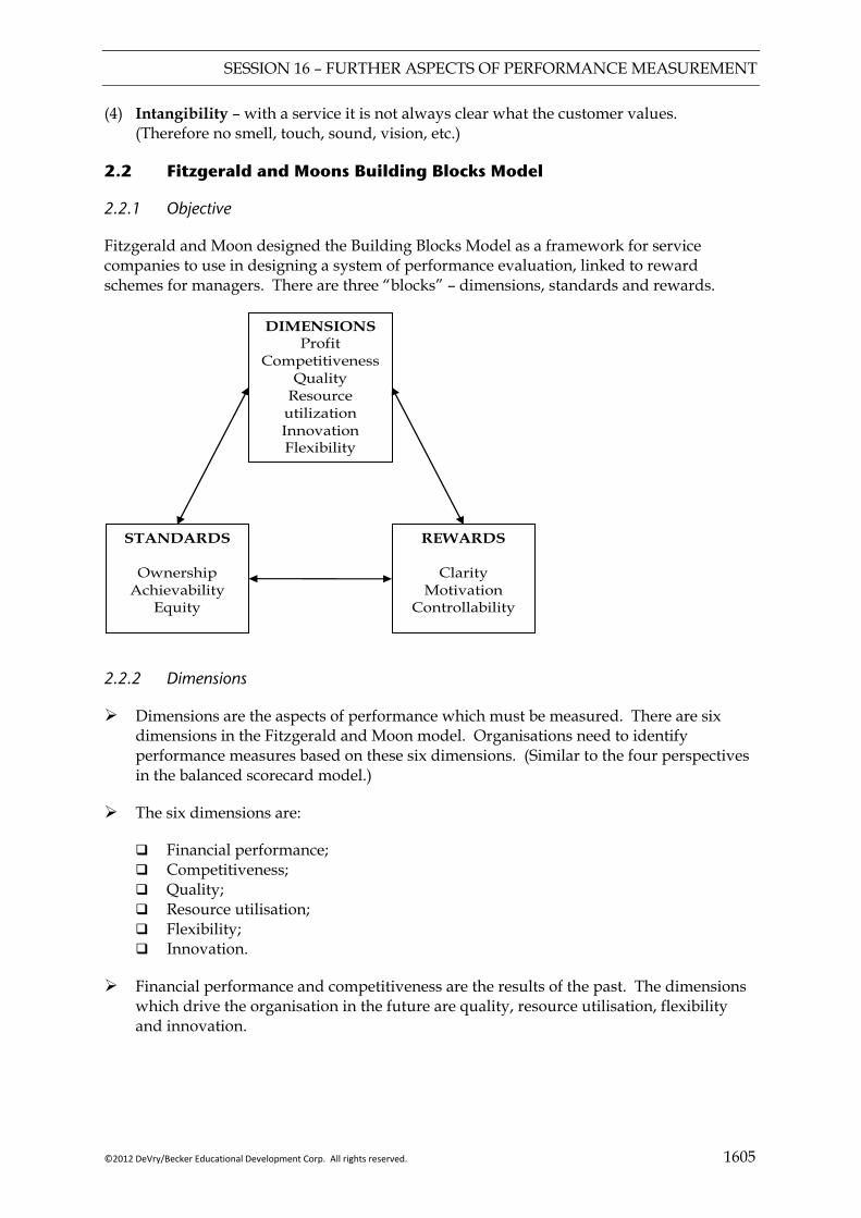
SESSION 16 – FURTHER ASPECTS OF PERFORMANCE MEASUREMENT
©2012 DeVry/Becker Educational Development Corp. All rights reserved. 1605
(4) Intangibility – with a service it is not always clear what the customer values. (Therefore no smell, touch, sound, vision, etc.)
2.2 Fitzgerald and Moons Building Blocks Model
2.2.1 Objective
Fitzgerald and Moon designed the Building Blocks Model as a framework for service companies to use in designing a system of performance evaluation, linked to reward schemes for managers. There are three “blocks” – dimensions, standards and rewards.
DIMENSIONS Profit
Competitiveness Quality
Resource utilization Innovation Flexibility
STANDARDS
Ownership Achievability
Equity
REWARDS
Clarity Motivation
Controllability
2.2.2 Dimensions
Dimensions are the aspects of performance which must be measured. There are six dimensions in the Fitzgerald and Moon model. Organisations need to identify performance measures based on these six dimensions. (Similar to the four perspectives in the balanced scorecard model.)
The six dimensions are:
Financial performance; Competitiveness; Quality; Resource utilisation; Flexibility; Innovation.
Financial performance and competitiveness are the results of the past. The dimensions which drive the organisation in the future are quality, resource utilisation, flexibility and innovation.
SESSION 16 – FURTHER ASPECTS OF PERFORMANCE MEASUREMENT
1606 ©2012 DeVry/Becker Educational Development Corp. All rights reserved.
Illustration 2
Additional research by Fitzgerald discovered the following methods of measuring the performance were being used by a car dealer in the UK:
Financial performance: profitability by dealer.
Competitiveness: market share & new car registrations by post code.
Quality of service: mystery customer, post transaction customer assessment.
Resource utilisation: sales per employee.
2.2.3 Standards
Having designed performance measures, targets should be set for managers based on these measures. Three principals should be applied here:
(1) Ownership – the managers should take ownership of (believe in) the targets. This is more likely to occur if the managers participate in setting them.
(2) Achievability – the targets should be challenging, but achievable; otherwise the managers will not be motivated.
(3) Equity – there will always be a conflict between what the business manager believes is achievable, and what the organisation believes is achievable. The business manager will always push for easier targets. Equity means than in setting targets, the organisation tries to be consistent across the different business areas in setting the difficulty of targets.
2.2.4 Reward schemes
Reward schemes may be linked to performance, with managers receiving bonuses if they achieve targets. Three principles apply:
(1) Clarity: The performance measurement scheme must be understood by employees.
(2) Motivation: Bonuses should be such that staff are motivated to achieve the targets.
(3) Controllability: Managers’ performance evaluation should only be judged on factors that they control.

SESSION 16 – FURTHER ASPECTS OF PERFORMANCE MEASUREMENT
©2012 DeVry/Becker Educational Development Corp. All rights reserved. 1607
3 NON-PROFIT SECTOR
3.1 Problems of identifying objectives in non-profit organisations
Non-profit organisations include:
Public sector bodies such as schools and hospitals Non-profit organisations (e.g. non-governmental organisations, NGOs)
Objectives of non-profit organisations are more difficult to ascertain for performance measurement systems because:
The objectives are difficult to quantify. If the objective of a hospital is to “improve health in the area,” how can this be measured?
Many non-profit bodies have multiple stakeholder, with different objectives, some of which may conflict:
Consider a state funded university as an example.
Principals
Students
Government
Employers
University management
Agent
The university management is accountable to multiple principles/stakeholders.
However the requirements of the principals may conflict. For example:
Students may desire small class sizes, large library, etc. Government wants to minimise costs per student.
Designing a performance measurement system where multiple and conflicting objectives exist is obviously very difficult.
Management must try to rank its principals/stakeholders and prioritise objectives.
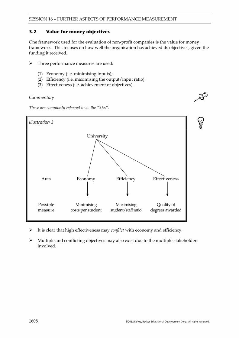
SESSION 16 – FURTHER ASPECTS OF PERFORMANCE MEASUREMENT
1608 ©2012 DeVry/Becker Educational Development Corp. All rights reserved.
3.2 Value for money objectives
One framework used for the evaluation of non-profit companies is the value for money framework. This focuses on how well the organisation has achieved its objectives, given the funding it received.
Three performance measures are used:
(1) Economy (i.e. minimising inputs); (2) Efficiency (i.e. maximising the output/input ratio); (3) Effectiveness (i.e. achievement of objectives).
Commentary These are commonly referred to as the “3Es”.
Illustration 3
University
Area Economy Efficiency Effectiveness
Possible measure
Minimising costs per student
Maximising student/staff ratio
Quality of degrees awarded
It is clear that high effectiveness may conflict with economy and efficiency.
Multiple and conflicting objectives may also exist due to the multiple stakeholders involved.
SESSION 16 – FURTHER ASPECTS OF PERFORMANCE MEASUREMENT
©2012 DeVry/Becker Educational Development Corp. All rights reserved. 1609
Example 1
In recent years there has been a considerable extension of management accounting into the public sector (e.g. hospitals and schools).
At the same time as management accounting was being introduced into these areas, many governments were specifying objectives for the public services, for example:
Hospitals –“to improve the standard of patient care” Schools –“to improve the quality of education”
Governments have also laid stress on the efficient use of resources in these areas.
Required:
Comment on the above objectives and assess the contribution that management accounting can make towards their achievement in the public sector.
4 EXTERNAL CONSIDERATIONS AND BEHAVIOUR ASPECTS
4.1 Behavioural aspects of performance management
Performance management is the whole process of identifying the objectives of the organisation, setting targets, measuring the performance against the targets, and taking action where targets have not been achieved, in an attempt to improve the performance of the organisation.
Managers need to be aware of the impact that performance management can have on the behaviour of the managers and staff whose behaviour is judged by the targets that were set.
4.1.1 Potential benefits of performance measurement systems
Managers and staff understand better the organisational objectives (e.g. increased market share) and will be motivated to contribute towards achieving them. This should help goal congruence.
Developing agreed measures of performance within the organisation (e.g. ROCE).
Allowing comparison of different organisations (e.g. ratio analysis).
Promoting accountability of the organisation to its stakeholders.

SESSION 16 – FURTHER ASPECTS OF PERFORMANCE MEASUREMENT
1610 ©2012 DeVry/Becker Educational Development Corp. All rights reserved.
4.1.2 Potential Problems
Tunnel vision – an obsession with maximising measured performance at the expense of non-measured performance. Staff may ignore important areas if they are not measured.
Myopia (short-sightedness) – maximising short run performance at the expense of long run success. For example, cutting back on staff training during recessions as this will mean the organisation is not well placed to take advantage of the later economic improvements.
Manipulation of data – “creative” reporting (e.g. trying to classify all adverse variances as planning variances).
“Gaming” (e.g. building slack into budgets).
Lack of goal incongruence (i.e. where the goals of the manager are not the same as the goals of the organisation). For example, if a manager is judged based on the ROCE of his division, he will reject projects which would reduce this, even if they might increase the overall return on capital employed of the company.
4.1.3 Solutions to the potential problems
Participation – involve staff at all levels in the design and implementation of the system.
Encourage a long term view among staff (e.g. through company share option scheme).
Ensure the system of performance evaluation is “audited” by experts to identify problems.
Review the system regularly.
Audit data used in performance measurement to prevent/detect manipulation.
4.2 External factors
Organisations do not exist in a vacuum, so performance measurement needs to take account of external factors as well as internal:
Stakeholders. A stakeholder is defined as any person or group that is affected by an organisation. Traditionally, performance measurement focussed only on one group of stakeholders; the owners of the organisation. Recently there has been recognition of the importance of other stakeholder groups.
Market/economic conditions. Account should be taken of the market conditions within which an organisation is operating when assessing its performance. When comparing two divisions for example, differences between the markets in which they exist should be taken into account.
Competitors – the performance of competitors will have a direct impact on the performance of an organisation. If competitors cut prices for example, this may impact on demand for the organisations own products.

SESSION 16 – FURTHER ASPECTS OF PERFORMANCE MEASUREMENT
©2012 DeVry/Becker Educational Development Corp. All rights reserved. 1611
Illustration 3
The following are the most common stakeholder groups, along with ways in which they can impact on the performance of an organisation:
Group Objectives Employees Satisfactory remuneration
Good working conditions
Customers Good quality products Suppliers Long term relationships Pay within agreed terms General public Potential employment Economic impact on region Environmental impact.
Government Compliance with law (e.g. environment)
4.3 Taking external considerations into account
4.3.1 Stakeholders
If the objectives of stakeholders are ignored, there may be adverse implications for the organisation. If staff salaries are too low for example, staff will become de-motivated, and good employees may leave the organisation. There could also be strikes. These factors could lead to poor customer service, which ultimately will affect the profits of the organisation.
Management needs to consider who are the most important stakeholders, and consider what their objectives are, and then identify ways to measure how these objectives are being met. Staff surveys for example are a common method used to assess staff satisfaction.
4.3.2 Market conditions and competitors
When assessing performance, account should be taken of factors that were outside of the control of the managers who are being assessed. This principal has already been discussed in the sessions on budgeting and variance analysis, so just to recap:
Budgets should be revised at the end of the year before being compared against actual performance, to take account of factors that are outside of the factors that occurred after the preparation of the original budget.
Standards can be revised to take into account changes in the environment. For example, the sales volume variance can be split into a market volume and market share variance.

SESSION 16 – FURTHER ASPECTS OF PERFORMANCE MEASUREMENT
1612 ©2012 DeVry/Becker Educational Development Corp. All rights reserved.
Generally speaking, performance measurement should be flexible enough to take into account external factors.
Example 2
The government of Northland privatised the Northland railway company in 2007. The company was split into smaller companies, each one operating the trains on a specific route. These companies were then sold to the private sector.
One of the private companies formed was the Great Suburban railway company, which provides passenger train services on a busy commuter route between the capital city of Bigton, and Smallton, a distance of 100 km.
Financial and other information relating to The great suburban railway for three different financial years are presented below.
2008 2009 2010 Revenue ($’000) 30,000 32,000 35,000 Profit ($’000) (1,000) 2,000 5,000 Number of passenger journeys (‘000) 2,000 1,900 1,900 Number of employees 500 450 400 %of trains arriving on time 70% 72% 75% Other information The Great Suburban Railway is the only company licensed to operate services on the route between Bigton and Smallton. The aims of privatisation of the trains were to stop the subsidy that the government had previously paid to the train company, and to increase the punctuality of services. Since privatisation, passengers have complained that the number of carriages on each train has been reduced, leading to a shortage of seats during peak times. Required:
Discuss the performance of The Great Suburban Railway from the perspective of: (a) a shareholder; (b) the government; (c) the population of Smallton.

SESSION 16 – FURTHER ASPECTS OF PERFORMANCE MEASUREMENT
©2012 DeVry/Becker Educational Development Corp. All rights reserved. 1613
Key points
The Balanced Scorecard Approach to performance measurement is aimed at ensuring that the various performance measures used support the overall strategy of the business.
The Balanced Scorecard looks at performance from four perspectives – Customer, Internal Processes, Learning and Growth and Financial.
Performance measurement in the Services sector is more difficult to measure than in manufacturing, due to:
Simultaneity; Perishability; Heterogeneity; Intangibility.
In the Fitzgerald and Moon Building Block model, performance in service businesses can be measured based on six dimensions:
Financial performance; Competitiveness; Quality of service; Resource utilisation; Flexibility; Innovation.
Performance measurement in non-profit organisations is more difficult due to:
Difficulty in quantifying the objectives Many stakeholders have interests in such organisations.
Performance measurement in the non-profit sector is often based around the “3Es” (i.e. economy, efficiency and effectiveness).
SESSION 16 – FURTHER ASPECTS OF PERFORMANCE MEASUREMENT
1614 ©2012 DeVry/Becker Educational Development Corp. All rights reserved.
FOCUS
You should now be able to:
explain and interpret the Balanced Scorecard and the Building Block model proposed by
Fitzgerald and Moon;
discuss the difficulties of target setting in qualitative areas;
comment on the problems of having non-quantifiable objectives in not for profit and public sector organisations;
explain hoe performance could be measured in the not for profit and public sectors;
comment on the problems of having multiple objectives in the not for profit and public sectors;
outline value for money as a public sector objective;
explain the causes and problems created by short-termism and financial manipulation of results and suggest methods to encourage a long term view;
explain the need to allow for external considerations in performance management, including stakeholders, market conditions and allowance for competitors;
suggest ways in which external considerations could be allowed for in performance management;
interpret performance in the light of external considerations;
identify and explain the behavioural aspects of performance measurement.
SESSION 16 – FURTHER ASPECTS OF PERFORMANCE MEASUREMENT
©2012 DeVry/Becker Educational Development Corp. All rights reserved. 1615
EXAMPLE SOLUTION
Solution 1
The objectives which are quoted in the question are so general that they do not provide a mechanism for judging how successful a hospital or a school has been regarding the attainment of those objectives.
The fact that the absence of a profit measure in Not-For-Profit (NFP) organisations causes problems for the measurement of their efficiency and effectiveness is widely acknowledged. However, management accountants are required to assist in the planning and controlling of the activities of organisations and to provide help and guidance to managers involved in decision-making processes regarding the deployment of resources available to the organisation. This is especially so in the case of NFP organisations where invariably a significant proportion of the cost base is fixed.
Economy can be defined as being “The terms and conditions under which the authority acquires human and material resources. An economical operation acquires resources of the appropriate quality and provides a service to the appropriate standard at the lowest cost”.
Effectiveness is defined as “The extent to which a programme achieves its established goals or other intended effects”.
Efficiency is defined as “The relationship between goods or services produced and resources used to produce them. An efficient operation produces the maximum output for any given set of resource input; or it has minimum input for any given quantity and quality of services provided”.
From the above definitions it can be seen that efficiency is the optimum of economy and effectiveness (i.e. the measure of output over input).
Consideration of the above “3Es” provides a clear understanding as to what governments mean by “the efficient use of resources in these areas”. The introduction of management accounting techniques within hospitals and schools has led managers to focus greater attention upon the achievement of economy, efficiency and effectiveness.
The principal problem, which is typical of schools and hospitals, lies in the difficulty in measuring the output (i.e. effectiveness) of such organisations.
In acknowledging that non-financial objectives can be more subjective than financial objectives when deciding whether they have been achieved, management accountants need to ensure the definition of organisational objectives in a manner which facilitates the measurement of the extent to which “patient care” and “quality of education” have been achieved.
Measurable objectives having been established, the management accountant should proceed to develop performance indicators which will serve as measurements of effectiveness, i.e. the extent to which the prescribed objectives have been met.
The management accountant will need to ensure that the control systems capture the information which will be used to assess the effectiveness of the organisation, and that any deficiencies in this respect are remedied.
SESSION 16 – FURTHER ASPECTS OF PERFORMANCE MEASUREMENT
1616 ©2012 DeVry/Becker Educational Development Corp. All rights reserved.
Solution 2
(a) From the perspective of shareholders
Shareholders will be pleased with the performance since privatisation. Revenues have increased by 16.67% between 2008 and 2010, which is good for a business such as railways where demand is likely to be limited. The reason for the increase would appear to be higher ticket prices, as the number of passenger journeys actually fell during the period.
While the company made a loss in 2008, the first year after privatisation, it made a good profit in 2009 and 2010. In fact profits have actually risen by more than revenue in absolute terms. This shows that the company has reduced costs at the same time as revenues are increasing. Net profit margin rose from 6.25% in 2009 to 14.2% in 2010.
It appears that the company has performed well from the perspective of shareholders.
(b) The government
The government will be pleased that it no longer has to subsidise the railway generally, so will be pleased that the company appears to be surviving in the private sector.
Another objective of privatisation was to increase the punctuality of trains. The Great Suburban railway has improved punctuality, measured as % of trains arriving on time, from 70% to 75% between 2008 and 2010, so some progress has been made. However, 25% of trains are still late, and the government (and passengers) will not be pleased with this.
(c) The population of Smallton
The main objective for the people of Smallton is likely to be having a reliable train service to the capital that charges reasonable prices.
Punctuality has already been discussed, and it is likely that passengers would be happy with the increase in the % of trains arriving on time although they would hope for further improvements in this area.
One area that customers are unlikely to be pleased about is the apparent increase in ticket prices. Dividing total revenue by number of passenger journeys, the average ticket per journey has risen from $15 in 2008 to $18.42 in 2010, and increase of 22%. This is a large increase, and is not likely to be popular, unless accompanied by better service in some way.
Customers are also complaining about the reduced number of carriages, leaving people without a seat during peak times. So it does not appear that passengers are experiencing a better service.
The number of passengers has fallen by 5% between 2010 and 2008. This is likely to be due to the increase in prices. People may be finding alternative ways to travel to the capital (such as by bus) or reducing their journeys.
Overall the population of Smallton are not likely to be happy with the performance of the privatised company.
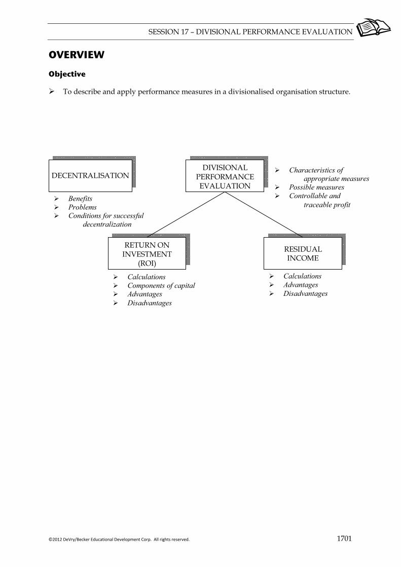
SESSION 17 – DIVISIONAL PERFORMANCE EVALUATION
©2012 DeVry/Becker Educational Development Corp. All rights reserved. 1701
OVERVIEW
Objective
To describe and apply performance measures in a divisionalised organisation structure.
DIVISIONAL PERFORMANCE EVALUATION
RESIDUAL INCOME
RETURN ON INVESTMENT
(ROI)
Characteristics of appropriate measures
Possible measures Controllable and
traceable profit
Calculations Components of capital Advantages Disadvantages
Benefits Problems Conditions for successful
decentralization
Calculations Advantages Disadvantages
DECENTRALISATION
SESSION 17 – DIVISIONAL PERFORMANCE EVALUATION
1702 ©2012 DeVry/Becker Educational Development Corp. All rights reserved.
1 DECENTRALISATION
Definition
Decentralisation is the delegation of authority to make decisions.
It requires the creation of autonomous business units or divisions.
These units can be:
Cost centres; Profit centres; Investment centres.
1.1 Benefits
Senior management can concentrate on strategy – the delegation of routine decision-making releases time for long-term corporate planning.
Faster decision-making – divisional managers are “on the spot” and can react quickly to changes.
Better decision-making – specialist managers are likely to understand their part of the business better than senior management.
Motivation – divisional managers are given responsibility and status and may increase effort.
Training and career progression – divisional managers acquire skills and experience which may prepare them for senior management (e.g. managers may be “rotated” between divisions).
Tax advantages – locating divisions in certain areas that enjoy tax incentives or government grants.
1.2 Problems
Lack of goal congruence – risk that divisional managers will make decisions not consistent with overall organisational objectives.
Increased information requirements – reporting systems must be introduced to monitor divisional performance.
Lost economies of scale – costs may rise through duplication of common activities. A central purchasing department may achieve better prices than divisional departments.
Loss of central control – top management loses control to divisional managers. Conflict may occur if top management disagrees with the decisions of divisional managers.

SESSION 17 – DIVISIONAL PERFORMANCE EVALUATION
©2012 DeVry/Becker Educational Development Corp. All rights reserved. 1703
1.3 Conditions for successful decentralisation
Successful
decentralisation
Carefully designed performance evaluation systems to reduce risk
of dysfunctional decisions
Business has several separate activities
Central policies to integrate and control eg major capital
expenditure, strategic decisions and transfer prices
Divisions should be independentfrom each other
2 DIVISIONAL PERFORMANCE EVALUATION
It is vital that senior management monitors the performance of divisions and divisional managers.
2.1 Characteristics of appropriate measures
Goal congruence – performance measures should encourage decisions consistent with company objectives.
Timeliness – performance reporting must be fast enough to allow any required corrective action.
Controllability – divisions and divisional managers should only be assessed on costs and revenues under their control.
2.2 Possible measures
The measures used will depend on the type of business unit being monitored.
It is dangerous to focus on one key measure of performance. A range of measures should be used to assess all elements of performance, both financial and non-financial – a “balanced scorecard” approach.
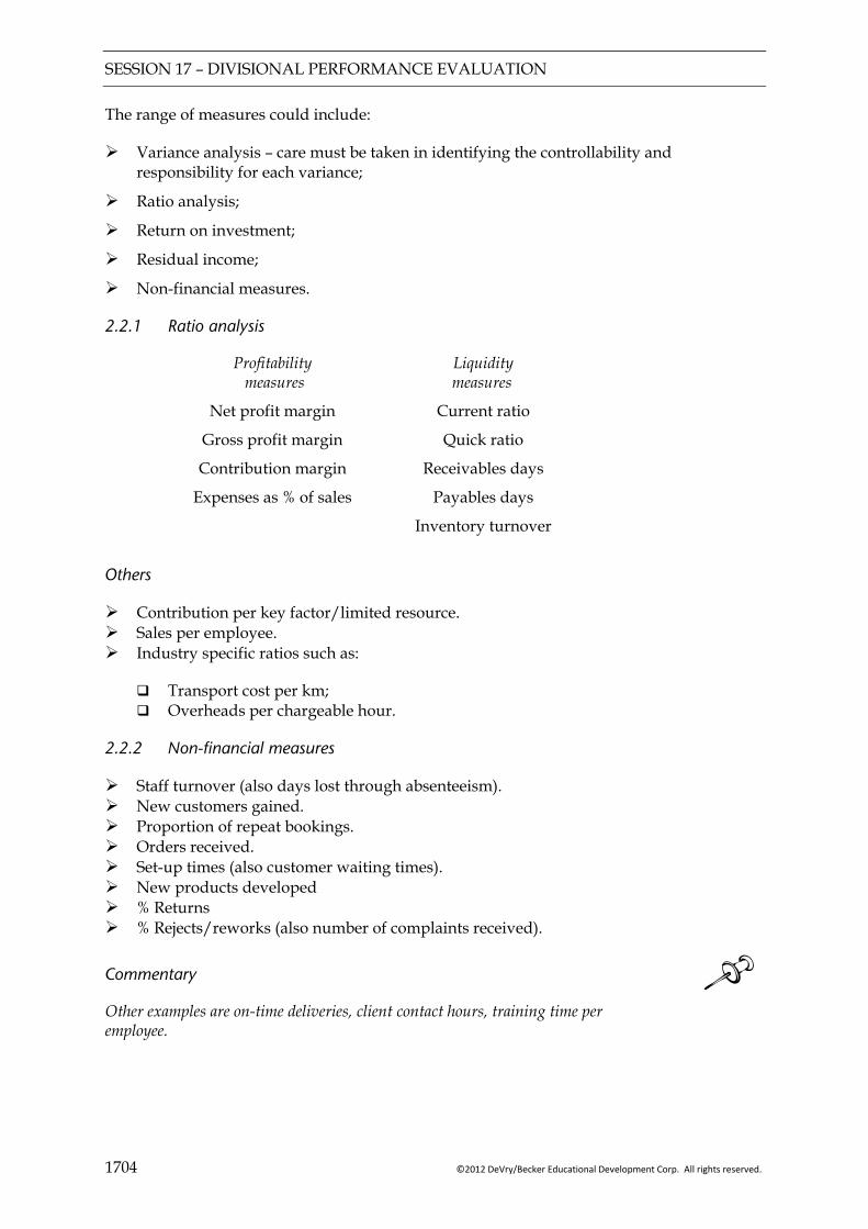
SESSION 17 – DIVISIONAL PERFORMANCE EVALUATION
1704 ©2012 DeVry/Becker Educational Development Corp. All rights reserved.
The range of measures could include:
Variance analysis – care must be taken in identifying the controllability and responsibility for each variance;
Ratio analysis;
Return on investment;
Residual income;
Non-financial measures.
2.2.1 Ratio analysis
Profitability measures
Liquidity measures
Net profit margin
Gross profit margin
Contribution margin
Expenses as % of sales
Current ratio
Quick ratio
Receivables days
Payables days
Inventory turnover
Others
Contribution per key factor/limited resource. Sales per employee. Industry specific ratios such as:
Transport cost per km; Overheads per chargeable hour.
2.2.2 Non-financial measures
Staff turnover (also days lost through absenteeism). New customers gained. Proportion of repeat bookings. Orders received. Set-up times (also customer waiting times). New products developed % Returns % Rejects/reworks (also number of complaints received).
Commentary Other examples are on-time deliveries, client contact hours, training time per employee.
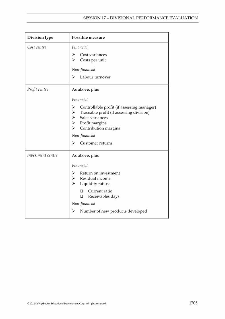
SESSION 17 – DIVISIONAL PERFORMANCE EVALUATION
©2012 DeVry/Becker Educational Development Corp. All rights reserved. 1705
Division type Possible measure
Cost centre Financial
Cost variances Costs per unit
Non-financial
Labour turnover
Profit centre As above, plus Financial
Controllable profit (if assessing manager) Traceable profit (if assessing division) Sales variances Profit margins Contribution margins
Non-financial
Customer returns
Investment centre As above, plus Financial
Return on investment Residual income Liquidity ratios:
Current ratio Receivables days
Non-financial
Number of new products developed
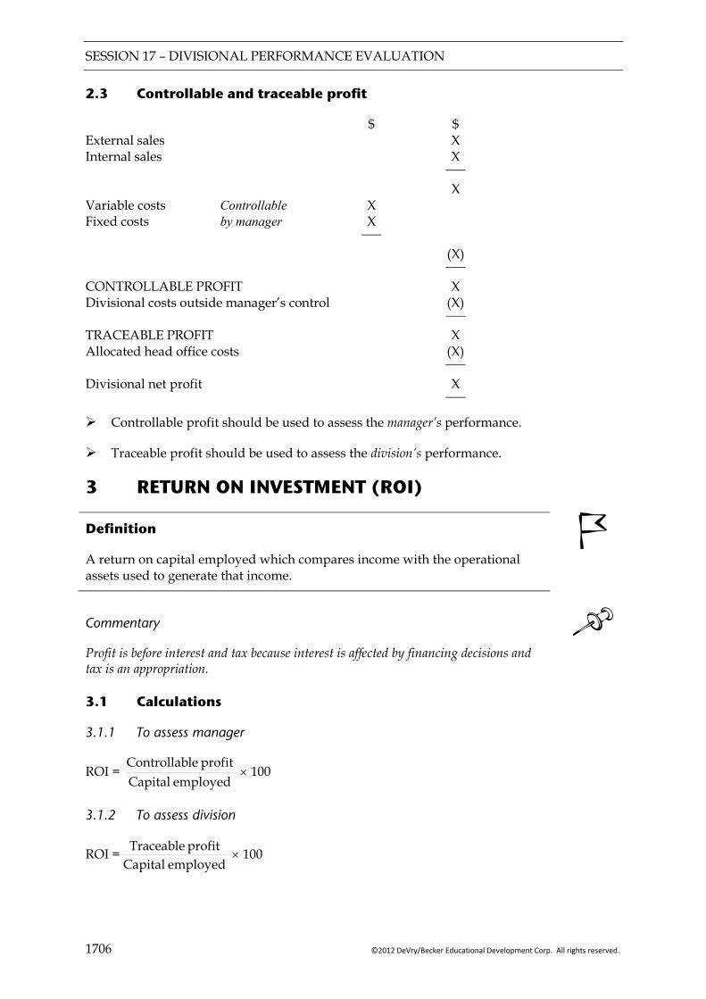
SESSION 17 – DIVISIONAL PERFORMANCE EVALUATION
1706 ©2012 DeVry/Becker Educational Development Corp. All rights reserved.
2.3 Controllable and traceable profit
$ $ External sales X Internal sales X ___
X Variable costs Controllable X Fixed costs by manager X ___ (X) ___ CONTROLLABLE PROFIT X Divisional costs outside manager’s control (X) ___ TRACEABLE PROFIT X Allocated head office costs (X) ___ Divisional net profit X ___
Controllable profit should be used to assess the manager’s performance.
Traceable profit should be used to assess the division’s performance.
3 RETURN ON INVESTMENT (ROI)
Definition
A return on capital employed which compares income with the operational assets used to generate that income.
Commentary Profit is before interest and tax because interest is affected by financing decisions and tax is an appropriation.
3.1 Calculations
3.1.1 To assess manager
ROI = employed Capital
profit leControllab × 100
3.1.2 To assess division
ROI =employed Capital
profit Traceable × 100
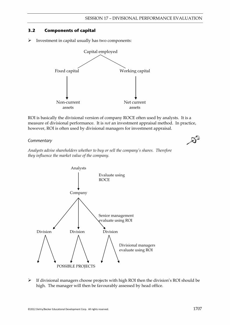
SESSION 17 – DIVISIONAL PERFORMANCE EVALUATION
©2012 DeVry/Becker Educational Development Corp. All rights reserved. 1707
3.2 Components of capital
Investment in capital usually has two components:
Capital employed
Fixed capital Working capital
Non-current assets
Net current assets
ROI is basically the divisional version of company ROCE often used by analysts. It is a measure of divisional performance. It is not an investment appraisal method. In practice, however, ROI is often used by divisional managers for investment appraisal.
Commentary Analysts advise shareholders whether to buy or sell the company’s shares. Therefore they influence the market value of the company.
Analysts
Evaluate using ROCE
Company
Senior management evaluate using ROI
Division Division Division
POSSIBLE PROJECTS
Divisional managers evaluate using ROI
If divisional managers choose projects with high ROI then the division’s ROI should be high. The manager will then be favourably assessed by head office.
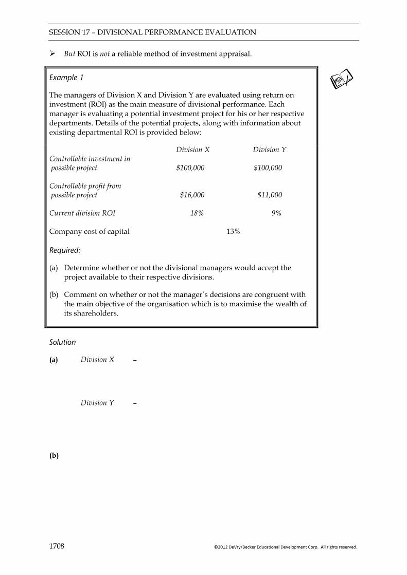
SESSION 17 – DIVISIONAL PERFORMANCE EVALUATION
1708 ©2012 DeVry/Becker Educational Development Corp. All rights reserved.
But ROI is not a reliable method of investment appraisal.
Example 1
The managers of Division X and Division Y are evaluated using return on investment (ROI) as the main measure of divisional performance. Each manager is evaluating a potential investment project for his or her respective departments. Details of the potential projects, along with information about existing departmental ROI is provided below:
Division X Division Y Controllable investment in possible project $100,000 $100,000 Controllable profit from possible project $16,000 $11,000 Current division ROI 18% 9% Company cost of capital 13% Required:
(a) Determine whether or not the divisional managers would accept the project available to their respective divisions.
(b) Comment on whether or not the manager’s decisions are congruent with the main objective of the organisation which is to maximise the wealth of its shareholders.
Solution
(a) Division X –
Division Y –
(b)
SESSION 17 – DIVISIONAL PERFORMANCE EVALUATION
©2012 DeVry/Becker Educational Development Corp. All rights reserved. 1709
3.3 Advantages
Relative measure – easy to compare divisions.
Similar to ROCE used externally by analysts.
Focuses attention on scarce capital resources.
Encourages reduction in non-essential investment by:
Selling off unused fixed assets; Minimising the investment in working capital.
Easily understood % (especially by non-financial managers).
3.4 Disadvantages
Risk of dysfunctional decision-making (Example 1).
Definition of capital employed is subjective. For example:
Should non-current assets be valued using:
(a) carrying amount (i.e. net book value); (b) historic cost; (c) replacement cost?
Should leased assets and intangible assets be included?
If net book value is used, ROI will become inflated over time due to depreciation (see later).
Risk of window-dressing; boosting reported ROI by:
Under investing; Cutting discretionary costs (particularly if ROI is linked to bonus systems).

SESSION 17 – DIVISIONAL PERFORMANCE EVALUATION
1710 ©2012 DeVry/Becker Educational Development Corp. All rights reserved.
4 RESIDUAL INCOME
Definition
Pre-tax profit less imputed interest charge for capital invested.
4.1 Calculations
4.1.1 For assessing manager $ Controllable profit X Imputed interest charge (X) ___
Residual income X ___ 4.1.2 For assessing division $ Traceable profit X Imputed interest charge (X) ___
Residual income X ___
4.1.3 Imputed interest
Imputed interest is notional interest charged on the division by head office.
Imputed interest = Capital employed × Interest rate
The company’s cost of capital is often used as the basis for the interest rate.
Example 2
The method of evaluating the performance of divisional managers has changed from return on investment to residual income. The two divisional managers are considering the investment projects considered in Example 1:
Division X Division Y Controllable investment in possible project $100,000 $100,000 Controllable profit from possible project $16,000 $11,000 Current division ROI 18% 9% Company cost of capital 13%
Required:
(a) What decision will the manager of each division make? (b) Is the decision-making goal congruent?
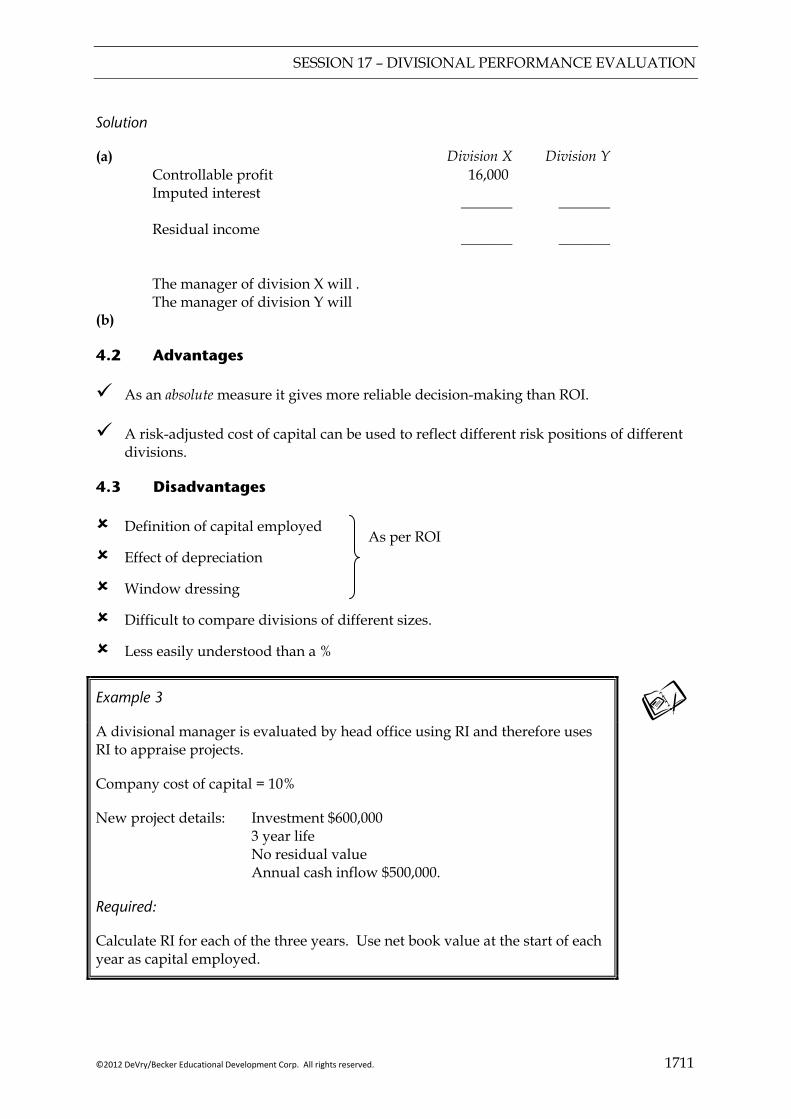
SESSION 17 – DIVISIONAL PERFORMANCE EVALUATION
©2012 DeVry/Becker Educational Development Corp. All rights reserved. 1711
Solution
(a) Division X Division Y Controllable profit
Imputed interest 16,000
Residual income
_______ _______
_______ _______
The manager of division X will .
The manager of division Y will (b) 4.2 Advantages
As an absolute measure it gives more reliable decision-making than ROI.
A risk-adjusted cost of capital can be used to reflect different risk positions of different divisions.
4.3 Disadvantages
Definition of capital employed
Effect of depreciation
Window dressing
Difficult to compare divisions of different sizes.
Less easily understood than a %
Example 3
A divisional manager is evaluated by head office using RI and therefore uses RI to appraise projects.
Company cost of capital = 10%
New project details: Investment $600,000 3 year life No residual value Annual cash inflow $500,000.
Required:
Calculate RI for each of the three years. Use net book value at the start of each year as capital employed.
As per ROI
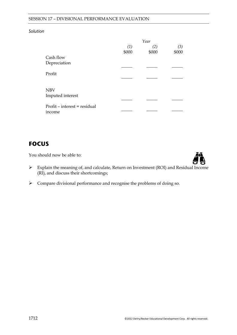
SESSION 17 – DIVISIONAL PERFORMANCE EVALUATION
1712 ©2012 DeVry/Becker Educational Development Corp. All rights reserved.
Solution
Year (1) (2) (3) $000 $000 $000 Cash flow
Depreciation
Profit
_____ _____
_____ _____
_____ _____
NBV
Imputed interest
Profit – interest = residual income
_____ _____
_____ _____
_____ _____
FOCUS
You should now be able to:
Explain the meaning of, and calculate, Return on Investment (ROI) and Residual Income
(RI), and discuss their shortcomings;
Compare divisional performance and recognise the problems of doing so.
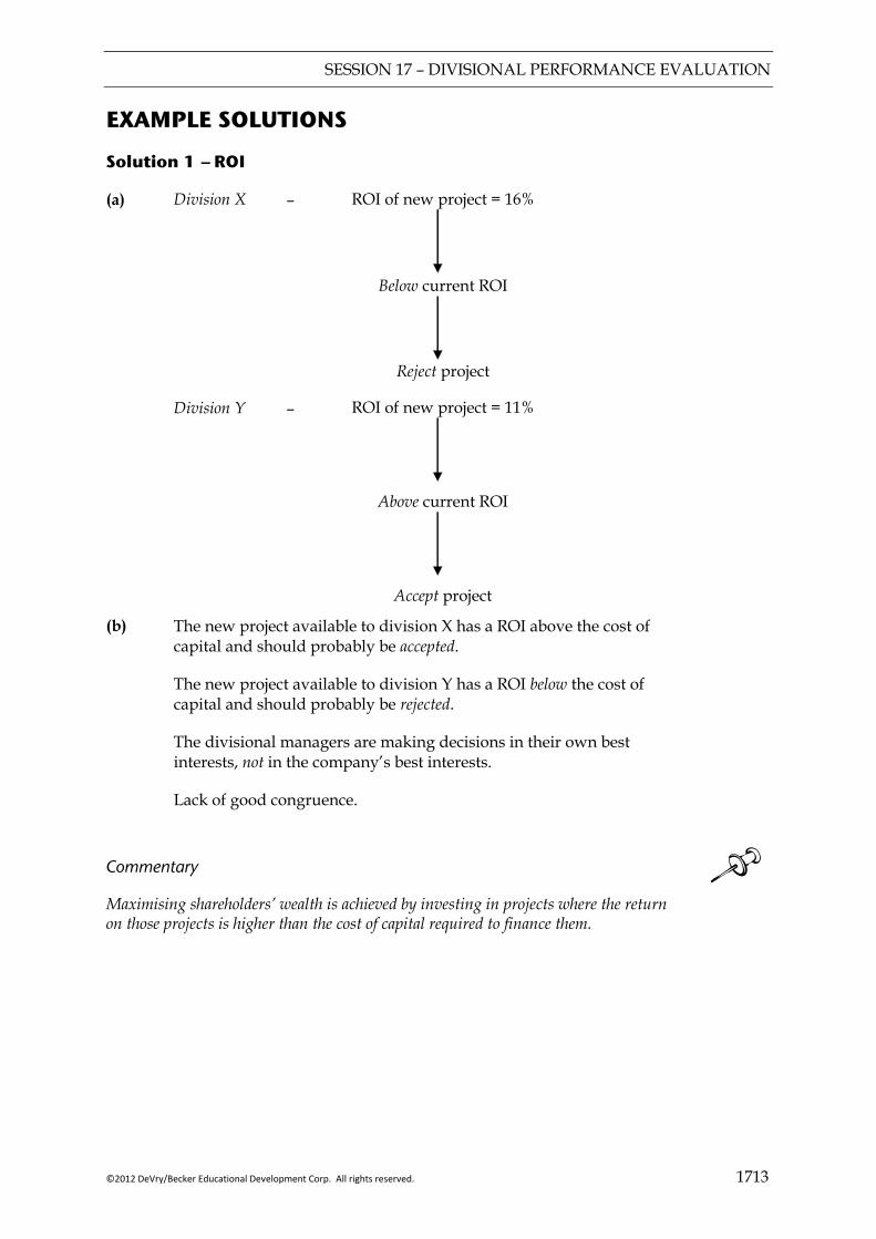
SESSION 17 – DIVISIONAL PERFORMANCE EVALUATION
©2012 DeVry/Becker Educational Development Corp. All rights reserved. 1713
EXAMPLE SOLUTIONS
Solution 1 — ROI
(a) Division X –
ROI of new project = 16%
Below current ROI
Reject project
Division Y –
ROI of new project = 11%
Above current ROI
Accept project (b) The new project available to division X has a ROI above the cost of
capital and should probably be accepted.
The new project available to division Y has a ROI below the cost of capital and should probably be rejected.
The divisional managers are making decisions in their own best interests, not in the company’s best interests.
Lack of good congruence.
Commentary Maximising shareholders’ wealth is achieved by investing in projects where the return on those projects is higher than the cost of capital required to finance them.

SESSION 17 – DIVISIONAL PERFORMANCE EVALUATION
1714 ©2012 DeVry/Becker Educational Development Corp. All rights reserved.
Solution 2 — Residual income
(a) Division X Division Y Controllable profit
Imputed interest 16,000
(13,000) 11,000
(13,000)
Residual income
_______ 3,000 _______
_______ (2,000) _______
The manager of division X will accept the project.
The manager of division Y will reject the project. (b) Yes Solution 3 — RI
Year (1) (2) (3) $000 $000 $000 Cash flow
Depreciation 500
(200) 500
(200) 500
(200)
Profit
____ 300 ____
____ 300 ____
____ 300 ____
NBV
Imputed interest 600
60 400
40 200
20
Profit – interest = residual income
____ 240 ____
____ 260 ____
____ 280 ____
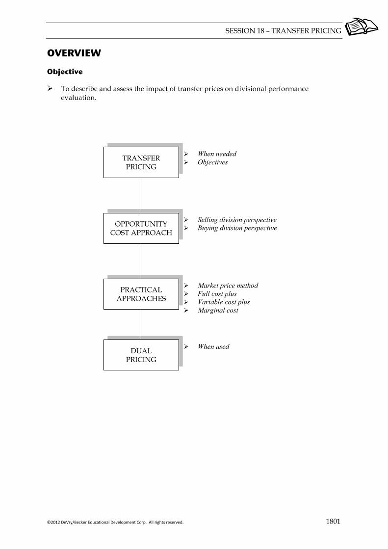
SESSION 18 – TRANSFER PRICING
©2012 DeVry/Becker Educational Development Corp. All rights reserved. 1801
OVERVIEW
Objective
To describe and assess the impact of transfer prices on divisional performance evaluation.
TRANSFER PRICING
OPPORTUNITY COST APPROACH
PRACTICAL APPROACHES
Selling division perspective Buying division perspective
When needed Objectives
Market price method Full cost plus Variable cost plus Marginal cost
DUAL PRICING
When used
SESSION 18 – TRANSFER PRICING
1802 ©2012 DeVry/Becker Educational Development Corp. All rights reserved.
1 TRANSFER PRICING
In an earlier session methods of setting prices for goods and services was discussed. This applied to prices for sales between independent parties.
In divisionalised organisations, the output of one department may form the input for another department. For the purpose of preparing management accounts for the two departments, which reflects the work performed by both divisions, a transfer pricing system is required.
Definition
A transfer price is the price at which goods or services are transferred from one division to another, within a company, or from one subsidiary to another within a group.
1.1 When needed
A transfer pricing policy is needed when:
An organisation has been decentralised into divisions; Inter-divisional trading of goods or services occurs.
Transfers between divisions must be recorded in monetary terms as revenue for supplying divisions and costs for receiving divisions.
Transfer pricing is more than just a bookkeeping exercise. It can have a large effect on the behaviour of divisional managers.
1.2 Objectives of transfer pricing
1.2.1 Goal congruence
Transfer prices should encourage divisional managers to make decisions that are in the best interests of the organisation as a whole.
In any divisionalised organisation there is a risk of dysfunctional decision making. Where inter-divisional trading occurs, this risk is particularly high.
Achievement of goal congruence must be the primary objective of a transfer pricing system.
Commentary Senior management must design a transfer pricing system which encourages divisional managers to make good decisions.

SESSION 18 – TRANSFER PRICING
©2012 DeVry/Becker Educational Development Corp. All rights reserved. 1803
Illustration 1
ABC Consulting has offices in several major cities in Eastern Europe. Sometimes consultants in one office work on projects for other offices. The transfer price charged is $1,100 per day of consulting.
The Managing Director of the Kyiv office of ABC Consulting discovered that he could hire reliable consultants on a freelance basis for $500 per day. On a recent project, in July, he used the services of a local freelance consultant for five days, paying $2,500 in total. “I’ve saved the Kyiv office $3,000!” he declared triumphantly at the end of the week.
During the week in question, the Moscow Office of ABC Consulting had a free consultant who could have done the work that the freelance consultant was hired to do. This consultant earns a fixed salary, so the additional cost to the company of this consultant working on the project in Kyiv would have been a flight ticket of $500 and accommodation of $500 in total.
The decision of the Managing Director of the Kyiv Office to hire the freelance consultant cost the ABC Group an additional $1,500 (the fee paid to the freelance consultant of $2,500 less the savings on travel and accommodation of $1,000).
This is an example of goal incongruence. The managing director of the Kyiv office has made a decision that is good for the Kyiv office, but not good for the overall group. The reason for this was that the internal transfer price was too high.
1.2.2 Divisional autonomy
Divisional managers should be free to make their own decisions. A transfer pricing system should eliminate the need for head office to tell divisions what to do.
Commentary Autonomy should improve motivation of divisional managers. 1.2.3 Divisional performance evaluation
Transfer prices should be “fair” and allow an objective assessment of divisional performance.
There is likely to be conflict between these objectives.
Key point
Goal congruence must take priority.
SESSION 18 – TRANSFER PRICING
1804 ©2012 DeVry/Becker Educational Development Corp. All rights reserved.
2 OPPORTUNITY COST APPROACH
2.1 Supplying division perspective
The minimum transfer price acceptable to the selling division is equal to:
Marginal (variable cost) + opportunity cost.
The opportunity cost is usually the lost contribution from external sales, either:
of the same product that is the subject of the transfer price; or of other products that the supplying division makes.
Scenario 1 — Opportunity cost is zero
When to use:
or capacity spare but market External
market external No and
sconstra intproduction No
In this situation opportunity cost is zero because internal transfers do not reduce contribution from external sales.
Example 1
Division Buy requires some components for its electronic games console. Division Sell has some spare capacity, and could make the components for a variable cost of $60 each. Required:
(a) Calculate the minimum transfer price acceptable to Division Sell.
(b) State what will happen if Division Buy can buy externally for $55.
(c) Conclude whether the actions of Division Buy and Division Sell in part (b) lead to goal congruence.
Solution
SESSION 18 – TRANSFER PRICING
©2012 DeVry/Becker Educational Development Corp. All rights reserved. 1805
Scenario 2 — Opportunity cost arises
Commentary An opportunity cost arises when an internal sale sacrifices an external sale.
When used:
external market exists
supplying division at full capacity. and
Example 2
Division Red makes product Y and product Z. The maximum capacity of the factory is 5,000 units per month in total. This capacity can be used to make either 5,000 units of product Y or 5,000 units of product Z, or any combination of the two. Y Z Selling price $12 $16 Variable cost $9 $11 Extra cost if sold externally $1 $1
____ ____ Contribution $2 $4
____ ____ Required:
(a) Determine which product Division Red would make, and what would be the monthly contribution of the division.
(b) Division Blue has asked Division Red to supply 1,000 units of Product Y per month. Determine the minimum transfer price that would be acceptable to Division Red.
(c) Division Blue now informs Division Red that it can buy product Y from an external supplier for $11 per unit and is not prepared to accept a price above this from Division Red.
Explain what would happen if both divisions were given autonomy to make their own decisions. Comment on whether this is acceptable to the company as a whole.
SESSION 18 – TRANSFER PRICING
1806 ©2012 DeVry/Becker Educational Development Corp. All rights reserved.
Solution
2.2 Buying division perspective
The maximum transfer price acceptable to the buying division will be the lower of:
External market price (if an external market exists);
The net revenue of the buying division.
The net revenue of the buying division means the ultimate selling price of the goods/ services sold by the buying division, less the costs incurred by the buying division.
Illustration 2
The bottling division of a large soft drinks manufacturer buys special syrup, made according to a secret recipe, from the syrup division. The bottling division adds carbonated water to the syrup to make the drink, bottles the drink, and sells it to the distributors.
Each bottle is sold for 50¢. The bottling division has calculated that the costs of making the drink and bottling it (excluding the cost of buying the syrup) are 20¢ per bottle. The net revenue of the bottling division is therefore 30¢ per bottle.
If the syrup division were to propose a transfer price in excess of 30¢ per bottle for the syrup, the bottling division would make a loss.
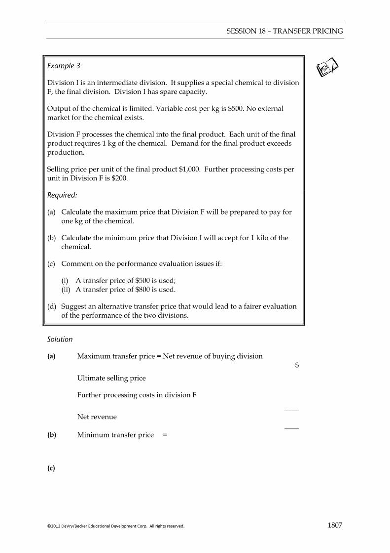
SESSION 18 – TRANSFER PRICING
©2012 DeVry/Becker Educational Development Corp. All rights reserved. 1807
Example 3
Division I is an intermediate division. It supplies a special chemical to division F, the final division. Division I has spare capacity.
Output of the chemical is limited. Variable cost per kg is $500. No external market for the chemical exists.
Division F processes the chemical into the final product. Each unit of the final product requires 1 kg of the chemical. Demand for the final product exceeds production.
Selling price per unit of the final product $1,000. Further processing costs per unit in Division F is $200.
Required:
(a) Calculate the maximum price that Division F will be prepared to pay for one kg of the chemical.
(b) Calculate the minimum price that Division I will accept for 1 kilo of the chemical.
(c) Comment on the performance evaluation issues if:
(i) A transfer price of $500 is used; (ii) A transfer price of $800 is used.
(d) Suggest an alternative transfer price that would lead to a fairer evaluation of the performance of the two divisions.
Solution
(a) Maximum transfer price = Net revenue of buying division $
Ultimate selling price
Further processing costs in division F
Net revenue
____
____ (b) Minimum transfer price =
(c)

SESSION 18 – TRANSFER PRICING
1808 ©2012 DeVry/Becker Educational Development Corp. All rights reserved.
3 PRACTICAL APPROACHES
3.1 Market price method
May be used if buying and selling divisions can buy/sell externally at market price.
However, the market price might need to be adjusted downwards if internal sales incur lower costs than external sales (e.g. due to lower delivery costs).
3.1.1 Advantages
Optimal for goal congruence if selling division is at full capacity. Encourages efficiency – supplying division must compete with external competition.
3.1.2 Disadvantages
Only possible if a perfectly competitive external market exists. Market prices may fluctuate.
3.2 Full cost plus
The supplying division charges full absorption cost plus a mark-up.
Standard costs should be used rather than actual to avoid selling divisions transferring inefficiencies to buying divisions.
3.2.1 Advantages
Easy to calculate if standard costing system exists. Covers all costs of selling division. May approximate to market price
3.2.2 Disadvantages
Fixed costs of selling division become variable costs of buying division – may lead to dysfunctional decisions.
If selling division has spare capacity it may lead to dysfunctional decisions.
Mark-up is arbitrary.
3.3 Variable cost plus
Similar to above – dysfunctional if spare capacity exists.
SESSION 18 – TRANSFER PRICING
©2012 DeVry/Becker Educational Development Corp. All rights reserved. 1809
3.4 Marginal cost
Marginal cost = variable cost + any incremental fixed costs e.g. stepped costs
3.4.1 Advantage
Optimal for goal congruence when:
Selling division has spare capacity; or No external market exists.
3.4.2 Disadvantage
May be difficult to calculate (variable cost is often used as an approximation).
3.5 Potential problem with all practical methods
All the practical methods suffer from a potential problem, which is that the price may lead to behaviour that is not goal congruent:
A price may be set that is too high for the buying division, leading the buying division to either buy externally or not to buy at all (and therefore to lose production).
Illustration 3
A selling division has spare capacity. It produces product B, which has a marginal cost of $10 per unit.
Another division within the company used product B in its production. The selling division can provide all of the supplies required by the buying division within its spare capacity. The buying division can also obtain supplies of product B externally for $15 per unit.
If a transfer price is set that is higher than $15 per unit, using any of the practical methods described above, then the buying division will buy externally.
This leads to an extra cost to the company overall of $5 per unit of product B since product B could be produced internally by the selling division for $10 per unit.
SESSION 18 – TRANSFER PRICING
1810 ©2012 DeVry/Becker Educational Development Corp. All rights reserved.
4 DUAL PRICING
4.1 When used
Dual pricing is sometimes used in situations where there is not a transfer price that would be acceptable to both the buying division and the selling division, so in the absence of intervention by head office, the two divisions would not trade with each other.
Head office may wish both divisions to trade for non-financial reasons, and may therefore use a system of dual pricing to encourage them to do so. Dual pricing works as follows:
A higher price is used when calculating the revenue of the selling division for goods supplied to the buying division.
A lower price is used when calculating the costs in the selling division for the goods supplied to it by the selling division.
Head office absorbs the difference between the two as a head office overhead.
FOCUS
You should now be able to:
Explain the basis for setting a transfer price using variable cost; full cost and the
principles behind allowing for intermediate markets;
Explain how transfer prices can distort the performance assessment of divisions and decisions made.
SESSION 18 – TRANSFER PRICING
©2012 DeVry/Becker Educational Development Corp. All rights reserved. 1811
EXAMPLE SOLUTIONS
Solution 1 — OTP = MC
(a) Minimum transfer price = marginal cost + Opportunity Cost, = $60 + $0. = $60.
Opportunity cost is $0 because the 500 units needed could be produced within the spare capacity of Division Sell.
(b) External price $55
Division Buy will buy externally. No transfer takes place.
(c) Both divisions are acting in a way that is in the best interests of the company overall. By buying externally for $55, Division Buy is saving the company $5 per component, since the cost to the company of making the components is $60.
Solution 2 — OTP = MC + Lost contribution
(a) Division Red would clearly make Product Z, as this generates the highest contribution per unit. Total contribution would therefore be $20,000 per month ($5,000 x 4).
(b) The minimum transfer price acceptable to Division Red for Product Y is:
$ Marginal (variable) cost 9 Opportunity cost 4 __
Minimum transfer price 13 __
The opportunity cost is the lost contribution per unit from selling Product Z.
(c) Division Red would refuse to sell for less than $13, so Division Blue would buy externally for $11 per unit.
Both divisions are acting in a way that is good for the organisation as a whole. Although the variable cost to the company of making Product Y is only $9, the opportunity cost of $4 is a real cost.
The cost to Division Red of producing Product Y, and therefore the cost to the company as a whole, is $13 per unit. By buying externally for $11, Division Blue is saving the company $2 per unit.

SESSION 18 – TRANSFER PRICING
1812 ©2012 DeVry/Becker Educational Development Corp. All rights reserved.
Solution 3 — Net revenue of buying division
(a) Maximum transfer price to division F = Net revenue $ Selling price 1,000
Further processing costs in division F (200)
Net revenue
____ 800 ____
The net revenue of $800 per kilo represents the maximum that Division F would be prepared to pay to Division I for the chemical. If the price exceeds this, then Division F will make a loss.
(b) Minimum price acceptable to Division I
$ Marginal (variable) cost per kilo 500 Opportunity cost 0 ___ Minimum transfer price 500 ___ (c) Performance evaluation
(i) If the minimum transfer price of $500 is used, then Division I will not make any profit.
(ii) If the maximum transfer price of $800 is used, then Division F makes no profit.
(d) Alternative transfer price
It can be seen that any transfer price between $500 and $800 per kilo would be acceptable to both parties. Without any further information about the nature of the production process and how much effort the two divisions, it is difficult to make a judgement about what would be a “fair” transfer price.
On suggestion might be to set a transfer price that is the midpoint between the minimum and maximum. This would be a price of $650 per kilo. If this were the case, both divisions could share the profits equally.

SESSION 19 – INDEX
©2012 DeVry/Becker Educational Development Corp. All rights reserved. 1901
A ABB 913 Activity based budgeting 205 Activity based costing 202 Activity based costing variances 1311 Activity-based budgeting 913 Additive model 1010 Apportionment 103 Avoidable costs 402
B Balanced scorecard 1602 Basic standard 922 Behaviour and standard costing 1411 Behavioural aspects of budgeting 920 Bottom up budgeting 908 Breakeven analysis 502 Breakeven chart 503 Breakeven point 502 Budget constrained 920 Budgeting 901 Business environment 302
C C/S ratio 507 Capacity variance 1209 Causes of variances 1214 Chance fork 807 Coefficient of determination 1006 Components of capital 1707 Constraints 606 Contribution 505 Control 103, 115 Control charts 1414 Controllability 1108 Controllable profit 1706 Corporate objectives 1502 Correlation 1021 Correlation coefficient 1005 Cost accounting 103 Cost plus pricing 702 Critical success factor 1511 Current ratio 1505 Current standard 922 Customer service 1513 Cyclical variation 1010
D Dead time 1315 Decentralisation 1702 Decision fork 807 Decision-making 103, 115 Demand 718 Demand curve 708 Deprival value 405 Detection costs 320 Dimensions 1605 Direct method 105 Divisional autonomy 1803 Divisional performance evaluation 1703 Downtime 1315 Dual price 613 Dual pricing 1810
E Economist’s model 708 Efficiency variance 1207, 1209 Elasticity of demand 709 Environmental ABC 321 Environmental costs 320 Environmental management accounting
318 Equity 1606 Expected standard 922 Expected value 802 Expenditure variance 1208 External failure costs 320
F Feasible region 607 Feedback 915 Feed-forward 915 Financial accounting 102 Financial performance indicators 1503 Fitzgerald & Moon 1605 Fixed costs 402, 502 Fixed overhead variances 1208 Fixed overheads 1107 Flexed budgets 918, 1109 Flexible budgets 918 Flow cost accounting 322 Focus groups 814 Forecasting 1004, 1014 Full cost plus 1808 Full cost plus pricing 702 Functional analysis 307
SESSION 19 – INDEX
1902 ©2012 DeVry/Becker Educational Development Corp. All rights reserved.
G Gearing ratio 1507 Geometric mean 1008 Goal congruence 1802 Goal incongruence 904 Going-rate pricing 717 Goldratt and Cox 314 Gross profit margin 1504
H Heterogeneity 1604 Hierarchy of objectives 1502 High-low method 1006 Hopwood 920
I Ideal standard 922, 1105 Idle time 1107 Idle time standards 1313 Idle time variance 1206 Imperfect competition 713 Incremental budgeting 911 Input output analysis 322 Intangibility 1605 Interdependence of variances 1217 Interest cover 1508 Internal failure costs 320 Investigation of variances 1413
J JIT 303 Just in time 303
K Kaplan and Norton 1602 Key factor analysis 311 Key performance indicators 1511
L Labour efficiency 1206 Labour variances 1206 Lagging indicators 1603 Leading indicators 1603 Learning curve 1015 Learning curves and variances 1316 Leverage 1507 Life cycle costing 308, 322 Limiting factors 602
Line of best fit 1003 Linear programming 605 Linear regression 1002, 1009 Liquidity ratio 1505 Loss leaders 717
M Make or buy 602, 619 Management accounting 102 Management charges 403 Margin of safety 508 Marginal cost 714, 1809 Marginal cost plus pricing 703 Marginal costing 1211 Marginal costing income statement 112 Marginal revenue 710 Market penetration 717 Market price method 1808 Market research 815 Market share variances 1410 Market skimming 717 Market volume variance 1409 Mass balance 322 Materials relevant cost 404 Materials variances 1205 Maximax 810 Maximin 810 McGregor, Douglas 909 Minimax regret 810 Mission 906 Mix and yield variances 1302 Motivation 902 Multi-limiting Factors 605 Multiplicative model 1011 Multi-product analysis 510
N Net profit margin 1504 Non-accounting style 920 Non-financial indicators 1511 Non-financial measures 1704 Non-profit sector 1607 Normal losses 1107
O Objective function 606 Operating statement 1210 Operating variances 1405 Operational NFPIs 1512
SESSION 19 – INDEX
©2012 DeVry/Becker Educational Development Corp. All rights reserved. 1903
Opportunity cost 403 Opportunity cost pricing 705 Outsourcing 602 Overhead rate variance 1207
P Payoff matrix 803 Perfect competition 713 Performance hierarchy 1502 Performance Hierarchy 905 Performance measurement 1502 Perishability 1604 Planning 102 Planning and operational variances 1403 Planning variances 1404 Pre-determined overhead rate 108 Prevention costs 320 Price discrimination 717 Price variance 1205 Pricing 701 Product costing 101 Product life cycle 719 Product-line pricing 718 Profit conscious 920 Profit margin 1504 Profit tables 803 Profit-volume chart 504
Q Quality indicators 1513 Quick Ratio 1506
R Reciprocal method 105 Regression analysis 1006 Relevant costs 402, 412 Replacement cost 404 Residual income 1710 Return on capital employed 1503 Return on investment 1706 Return on investment pricing 703 Reverse engineering 307 Reward schemes 1606 Risk 802 Risk and uncertainty 801 Risk seeker 810 ROI 1706 Rolling 909 Rule of thumb models 1414
S Sales margin mix variances 1308 Sales margin quantity variances 1309 Sales volume variance 1204, 1409 Scarce resources 403 Scatter diagram 1002 Seasonal variation 1009 Sensitivity analysis 811 Service departments 104 Service industries 306, 1604 Setting standards 1105 Shadow price 613 Shut-down decisions 409 Simulation 813 Simultaneity 1604 Simultaneous equations 608 Slack 615 Spreadsheets 1019 Spurious correlation 1005 Stages in budgetary control 902 Standard cost 609 Standard cost card 111 Standard costing systems 1104 Standard costs 1102 Standards 922 Step down method 105
T Target cost gap 307 Target costing 304 Target profits 506 Target return 703 Target setting 1513 Tear down analysis 307 Theory of constraints 313 Theory X 909 Throughput accounting 311 Throughput accounting ratio 317 Throughput contribution 315 Time series analysis 1008 Top down budgeting 908 Total absorption costing 115 Total quality management 302 TPAR 317 TQM 302 Traceable profit 1706 Transfer pricing 1801 Trend 1009
SESSION 19 – INDEX
1904 ©2012 DeVry/Becker Educational Development Corp. All rights reserved.
U Uncertainty 802 Uncontrollable costs 403 Usage variance 1205
V Value engineering 307 Value for money 1608 Value of perfect information 804 Variable costs 502 Variable overhead variances 1207 Variable overheads 1107 Variance analysis 1202 Volume discounting 718 Volume variance 1208, 1209
W Waste 1107
Z ZBB 911 Zero-based budgeting 911
ABOUT BECKER PROFESSIONAL EDUCATION
Together with ATC International, Becker Professional Education
provides a single destination for candidates and professionals
looking to advance their careers and achieve success in:
• Accounting
• International Financial Reporting
• Project Management
• Continuing Professional Education
For more information on how Becker Professional Education can
support you in your career, visit www.becker.com.
®

®
©2012 DeVry/Becker Educational Development Corp. All rights reserved.
www.beckeratci.com | [email protected]
®
This ACCA Study System has undergone a Quality Assurance review by ACCA and includes:
• An introductory session containing the ACCA Syllabus and Study Guide and approach to examining
the syllabus to familiarize you with the content of this paper
• Coverage of the core syllabus areas
• A visual overview at the beginning of each session showing how topics are related
• Definitions of terms
• Illustrations
• Examples with solutions
• Key points drawing attention to rules, underlying concepts and principles
• Commentaries providing additional information
• Focus on learning outcomes
• A bank of practice questions
Related Documents


