Paper deinterlace stim

2476 IEEE TRANSACTIONS ON IMAGE PROCESSING, VOL. 16, NO. 10, OCTOBER 2007

An Inpainting- Based Deinterlacing MethodColoma Ballester, Marcelo Bertalmío, Vicent Caselles, Associate Member, IEEE, Luis Garrido,

Adrián Marques, and Florent Ranchin

Abstract—Video is usually acquired in interlaced format, whereeach image frame is composed of two image fields, each fieldholding same parity lines. However, many display devices requireprogressive video as input; also, many video processing tasksperform better on progressive material than on interlaced video.In the literature, there exist a great number of algorithms forinterlaced to progressive video conversion, with a great tradeoffbetween the speed and quality of the results. The best algorithmsin terms of image quality require motion compensation; hence,they are computationally very intensive. In this paper, we proposea novel deinterlacing algorithm based on ideas from the imageinpainting arena. We view the lines to interpolate as gaps that weneed to inpaint. Numerically, this is implemented using a dynamicprogramming procedure, which ensures a complexity of ( ),where is the number of pixels in the image. The results obtainedwith our algorithm compare favorably, in terms of image quality,with state-of-the-art methods, but at a lower computational cost,since we do not need to perform motion field estimation.

Index Terms—Geometry, interpolation, interlacing, inpainting,video restoration.

I. INTRODUCTION

I NTERLACED scanning is a sampling method for video se-quences. In interlaced scanning, the scene is captured by

sampling iteratively a set of odd and even fields. The even fieldholds the even lines of the frame, the odd field holds the oddlines of the frame. These fields are captured successively at regu-larly spaced time intervals. Since the invention of TV in the early1930s, the interlaced scan has been adopted by many broad-casting systems such as PAL, NTSC, or SECAM, and can beconsidered the result of a tradeoff between vertical resolutionand frame rate and transmission bandwidth requirements. In-deed, interlacing is a way of doubling the frame rate by halvingthe vertical resolution.

Early TV displays, based on cathode ray tube technology,were designed to work with an interlaced input. The low-passfilter response of the human eye and the one of the phosphor at

Manuscript received October 17, 2006; revised May 23, 2007. This workwas supported in part by the IP-RACINE Project IST- 511316. C. Ballester,M. Bertalmío, and V. Caselles were supported by the PNPGC project, refer-ence MTM2006-14836. M. Bertalmío and L. Garrido were supported by theRamón y Cajal Program. V. Caselles was supported by the Departament d’Uni-versitats, Recerca i Societat de la Informació de la Generalitat de Catalunya.The associate editor coordinating the review of this manuscript and approvingit for publication was Dr. Dimitri Van De Ville.

The authors are with the Departament de Tecnologia, UniversitatPompeu Fabra, Barcelona, Spain (e-mail: [email protected];[email protected]; [email protected]; [email protected];[email protected]; [email protected]).

Color versions of one or more of the figures in this paper are available onlineat http://ieeexplore.ieee.org.

Digital Object Identifier 10.1109/TIP.2007.903844

the display allowed to reduce annoying effects due to the sam-pling method. Nowadays, many displays based on novel tech-nologies such as liquid crystal or plasma do need a full frameas input. If these devices receive an interlaced signal, it must beconverted to progressive before it can be displayed.

Interlaced-to-progressive conversion (IPC) approaches allowus to convert interlaced material into a progressive one. Pro-gressive material is not only necessary for display in progres-sive devices, but also because some image processing tasks mayrequire progressive video. IPC can be accomplished through aprocess that, for each field, doubles the vertical resolution usingas input only the lines of the current field—intraframe recon-struction—or the lines of previous and following fields—inter-frame reconstruction.

There is a vast number of techniques in the field of IPC,techniques which can be based on intraframe reconstructionmethods, interframe reconstruction methods, or a combinationof both. There is an important tradeoff between speed andquality with these algorithms: the algorithms that introduceless visual artifacts require motion compensation (MC), whichis a computationally very intensive procedure (implying thecomputation of motion vectors for every pixel). On the otherhand, among the algorithms that do not require MC, some of thebest ones are directional interpolators, which make use of theedge information to decide, for each missing pixel, the spatialand/or temporal direction in which interpolation takes place.Directional interpolators have varied problems such as beingsensitive to noise, only being able to detect a limited numberof orientations or having problems to reconstruct periodicstructures. More importantly, they all decide the interpolationdirection on a very local basis, that is, the decision on the inter-polation direction for each missing pixel is done independentlyof the decision done for neighboring pixels. This sometimesresults in very noticeable visual artifacts.

Our main contribution in this paper is a novel deinterlacingalgorithm that does not require MC though it may be comple-mented with it. Our approach is based on variational inpaintingtechniques [26], [27] and may be interpreted as a way of per-forming directional interpolation but with a global (instead oflocal) optimization criterion which takes into account the or-dered structure of the level sets of the image. Our experimentsshow that it can be favorably compared both quantitatively andqualitatively with most MC deinterlacing techniques, which arethe state-of-the-art algorithms in the literature.

The outline of the paper is as follows. In Section II, we re-view the most common strategies used for deinterlacing. In Sec-tion III, we review the basic idea involving the combination ofseveral interpolation methods to produce a new and more ro-bust one. In Section IV-A, we explain the main ideas behindgeometric inpainting methods and we propose our deinterlacing

1057-7149/$25.00 © 2007 IEEE

BALLESTER et al.: INPAINTING-BASED DEINTERLACING METHOD 2477

method: we compute a spatial interpolation, a temporal interpo-lation and we combine both of them. In Section V, we displaythe results of our experiments and we compare our method withother algorithms proposed in the literature. We also compareour method with the combination of it with MC deinterlacing,showing that the gain in quality is very little. Our conclusionsare summarized in Section VI.

II. CURRENT IPC APPROACHES

This section is devoted to a brief description of some of themethods available for IPC. They range from the very simple lineaveraging to more complex IPC based on MC. All the methodsdescribed here have been implemented in our paper in orderto benchmark them against our proposal. In this paper, we di-vide the IPC methods into four classes: linear methods, direc-tional interpolators, motion-adaptive IPC, and motion-compen-sated IPC. We will describe with some more detail the direc-tional interpolators, since they are related to our approach.

To fix the notation, throughout this paper de-notes an interlaced sequence, where

corresponds to the pixel coor-dinates, and to the time sample ( arepositive integers). The size of corresponds to the size associ-ated to the full progressive frame. Thus, we are assuming thatin even fields of the even lines are defined whereas the oddlines are not, and that in odd fields of the odd lines are definedwhereas the even lines are not. Notice that, as an interpolationprocess, the output of a deinterlacer is constructed by filling thevalues of the missing pixels using the known pixel values of .

A. Linear Methods

These methods perform linear operations on the interlacedmaterial in order to double the vertical resolution. The termlinear stems from the fact that the interpolated pixel is obtainedby a linear combination of spatiotemporal neighboring pixels.Some IPC methods that can be included in this class are as fol-lows (see [35] and references therein).

• Line Doubling: As its name indicates, interpolation is per-formed by doubling each line. The resulting sequence’svertical resolution is half of the original and usually suf-fers from severe flickering.

• Line Average: Each missing pixel is interpolated by aver-aging the upper and lower pixel in the spatial direction, i.e.,using the formula

(1)

The resulting sequence still suffers from annoying arti-facts, specially in regions with fine vertical details.

• Field Weaving: It corresponds to the temporal version ofthe line doubling method. Each missing pixel is copiedfrom the previous frame at the sample pixel coordinate,

. Field weaving allows perfectreconstruction of the missing lines for static areas, but veryannoying artifacts may appear in moving areas.

• Field Averaging: It is the temporal analogous of line aver-aging. In this case the missing pixels are interpolated lin-early between neighboring temporal samples

(2)

Similar effects as for field weaving may appear with thistechnique.

• Vertical-Temporal (VT) Filtering: In this case, the impulseresponse of the filter has support in the space-time domainand is designed to avoid motion artifacts, but it is difficultto keep vertical detail when high temporal frequencies arepresent (see [13] and references therein).

B. Directional Interpolation Methods

These methods try to use the edge information present in thescene for a proper reconstruction of the progressive frame. Foreach missing pixel, the neighboring spatiotemporal pixels areanalyzed and a decision on the direction in which interpolationshould be done is taken. Some of the IPC methods that are in-cluded into the class of directional interpolators are as follows.

• Edge-Based Line Average (ELA) [14]: For each missingpixel, an estimation of the direction of the edge passingthrough it is performed based on the correlation of lumi-nance values of the 3 3 window centered around it. If

is the pixel to interpolate, the interpolation direc-tion is estimated by evaluating the three pixel differences

, ,and . The pixelis then linearly interpolated between the pair of pixels thatresults in the lowest pixel difference.Compared to linear approaches, ELA may reconstructsharply oblique lines, avoiding many of the jagged edgesproduced by line doubling or line averaging. However,ELA still produces noticeable flicker. Moreover, due tothe very limited number of directions considered withthis algorithm, ELA may incorrectly estimate the edgedirection, thereby assigning to the missing pixel a valuethat stands out as incorrect and is, thus, also clearly visible.

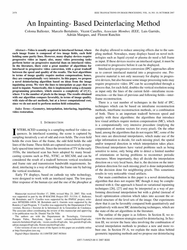
• Direction Oriented Interpolation [40] (DOI): This ap-proach tries to determine the orientation of the edge at amissing pixel in a more robust manner than ELA does.For that purpose, instead of computing simple pixel differ-ences to estimate the edge orientation as ELA does, a setof windows centered at the corresponding pixels are used.As shown in Fig. 1, three windows are used: one window

centered at the missing pixel, and two sliding windowsand . By comparing the pixels of and , and

the pixels of and , the edge direction can be deter-mined, and, thus, the missing pixel may be interpolated.Even if DOI is more robust than ELA, our experimentsshow that DOI may produce annoying artifacts in periodicstructures.

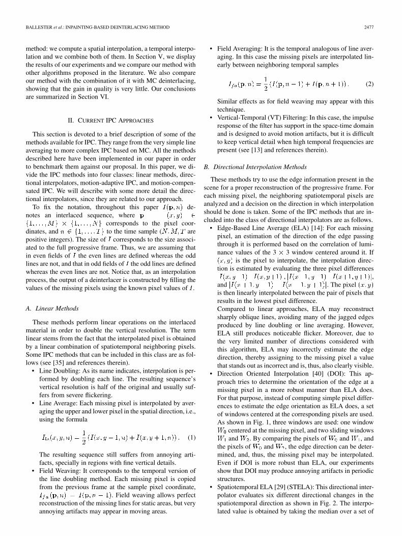
• Spatiotemporal ELA [29] (STELA): This directional inter-polator evaluates six different directional changes in thespatiotemporal direction as shown in Fig. 2. The interpo-lated value is obtained by taking the median over a set of


Fig. 1. Reference windows in DOI approach.

Fig. 2. STELA spatiotemporal window.

values obtained from the pixel differences. STELA outper-forms the previously presented directional interpolators inslow or static areas since it is exploiting temporal informa-tion in addition to the spatial one to which the ELA andDOI are restricted.

• Structure Tensor Edge Orientation Estimation [36]: In[36], the authors considered the problem as an inpaintingproblem and proposed a spatial interpolation along theedge directions, which were estimated in a robust wayusing the structure tensor, combined with a MC interpola-tion using the result of the first spatial step.

Many other variants of these ideas have been proposed (see[15], [23], and [31]).

C. Motion Adaptive Methods

Spatial deinterlacing techniques exploit the correlation be-tween neighboring samples in a field and, thus, work properlyin the case that there are no vertical details appearing. Temporaldeinterlacing techniques exploit the correlation in the temporaldomain and, thus, work properly in the absence of motion.

Motion adaptive methods aim at exploiting the best of bothtypes of methods. As we have said, their performance dependson the presence or absence of motion. For instance, fieldweaving behaves well in areas where no motion is presentwhereas line averaging behaves better than weaving in movingareas. Thus, the main issue in motion adaptive IPC methods isthe robust detection of moving parts of the image.

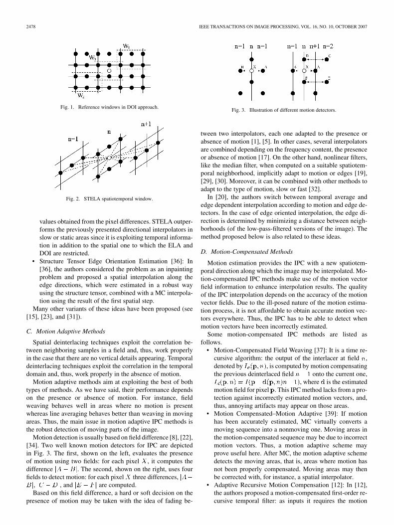
Motion detection is usually based on field difference [8], [22],[34]. Two well known motion detectors for IPC are depictedin Fig. 3. The first, shown on the left, evaluates the presenceof motion using two fields: for each pixel , it computes thedifference . The second, shown on the right, uses fourfields to detect motion: for each pixel three differences,

, , and are computed.Based on this field difference, a hard or soft decision on the

presence of motion may be taken with the idea of fading be-

Fig. 3. Illustration of different motion detectors.

tween two interpolators, each one adapted to the presence orabsence of motion [1], [5]. In other cases, several interpolatorsare combined depending on the frequency content, the presenceor absence of motion [17]. On the other hand, nonlinear filters,like the median filter, when computed on a suitable spatiotem-poral neighborhood, implicitly adapt to motion or edges [19],[29], [30]. Moreover, it can be combined with other methods toadapt to the type of motion, slow or fast [32].

In [20], the authors switch between temporal average andedge dependent interpolation according to motion and edge de-tectors. In the case of edge oriented interpolation, the edge di-rection is determined by minimizing a distance between neigh-borhoods (of the low-pass-filtered versions of the image). Themethod proposed below is also related to these ideas.

D. Motion-Compensated Methods

Motion estimation provides the IPC with a new spatiotem-poral direction along which the image may be interpolated. Mo-tion-compensated IPC methods make use of the motion vectorfield information to enhance interpolation results. The qualityof the IPC interpolation depends on the accuracy of the motionvector fields. Due to the ill-posed nature of the motion estima-tion process, it is not affordable to obtain accurate motion vec-tors everywhere. Thus, the IPC has to be able to detect whenmotion vectors have been incorrectly estimated.

Some motion-compensated IPC methods are listed asfollows.

• Motion-Compensated Field Weaving [37]: It is a time re-cursive algorithm: the output of the interlacer at field ,denoted by , is computed by motion compensatingthe previous deinterlaced field onto the current one,

, where is the estimatedmotion field for pixel . This IPC method lacks from a pro-tection against incorrectly estimated motion vectors, and,thus, annoying artifacts may appear on those areas.

• Motion Compensated–Motion Adaptive [39]: If motionhas been accurately estimated, MC virtually converts amoving sequence into a nonmoving one. Moving areas inthe motion-compensated sequence may be due to incorrectmotion vectors. Thus, a motion adaptive scheme mayprove useful here. After MC, the motion adaptive schemedetects the moving areas, that is, areas where motion hasnot been properly compensated. Moving areas may thenbe corrected with, for instance, a spatial interpolator.

• Adaptive Recursive Motion Compensation [12]: In [12],the authors proposed a motion-compensated first-order re-cursive temporal filter: as inputs it requires the motion


Fig. 4. Pseudocode for the deinterlacing algorithm proposed in this paper.

field and the output of an initial dein-terlacing algorithm (like line averaging). Assuming thatthe previous field has already been deinterlaced,i.e., we have , then the deinterlaced value at

is computed as a weighted averaging of the valuesof (resp., ) and if

(resp., ).The weighting parameters are adaptive and are designed soas to reduce nonstationarities along the motion trajectory.

E. Discussion

As can be seen, there exist a large pool of approaches for IPC.Our experiments show that the best results are obtained withmotion-compensated methods, which are computationally quiteintensive.

On the other hand, and as we described above, the direc-tional interpolators decide the interpolation direction using thevalues of neighboring pixels of the missing pixel. However,there is no constraint for edge directions of neighboring pixelsand edges may cross. This is, according to our experiments, themain reason why these methods fail to properly reconstruct themissing pixels.

Our purpose in this paper is to develop a new and robust di-rectional interpolator that takes into account the fact that levellines of the image do not cross. This geometric property is im-posed as a global optimization constraint. With this, most of theannoying artifacts of local directional interpolators are avoided.Moreover, our interpolator is applied both in the spatial and tem-poral domain and, as a result, our IPC does not need to rely onMC to obtain good results.

III. COMBINING SEVERAL INTERPOLATION METHODS

The combination of several IPC methods proposed in [12]leads to an improved result. In a further development of thisidea, in [21], Kovacevic et al. proposed an algorithm for dein-terlacing video sequences by weighting several interpolationmethods. The basic idea is to combine several interpolationmethods in a recursive way using successive approximations.

The first level of approximation [21] consists in combiningthe result of two simple interpolation methods, line and fieldaveraging methods using a linear combination with

weights which depend on the relia-bility of the method

(3)

where . The weight [resp.,] is larger when the neighborhoods of pixels

and [resp., of pixels and ]are similar where the similarity of two neighborhoods is mea-sured by a (weighted) distance. In other words, the coeffi-cients are an increasing function of the reliability of the method,the reliability being an increasing function of the similarity [seethe weights in formula (5)]. We shall keep this basic rule in whatfollows and in our deinterlacing method below.

In the second level of approximation [21], the result of thefirst level is used to compute the edge direction(using steerable filters) on pixel of frame and then computean edge-based line average interpolation . Then the authorscombine the results and using a weighted averagewhere the weight given to each term depends on its reliability.Let be the image obtained.

The third level of approximation [21] uses to compute aforward and backward motion estimation ,

, which are used to interpolate a new image in a recursiveway

where , are weight factors which depend onthe reliability of the motion estimates. The final deinterlacedsequence is obtained as a weighted average of the images ,

, , with coefficients depending on the reliability ofthe estimate, giving more weight to the more reliable ones (see[21]).

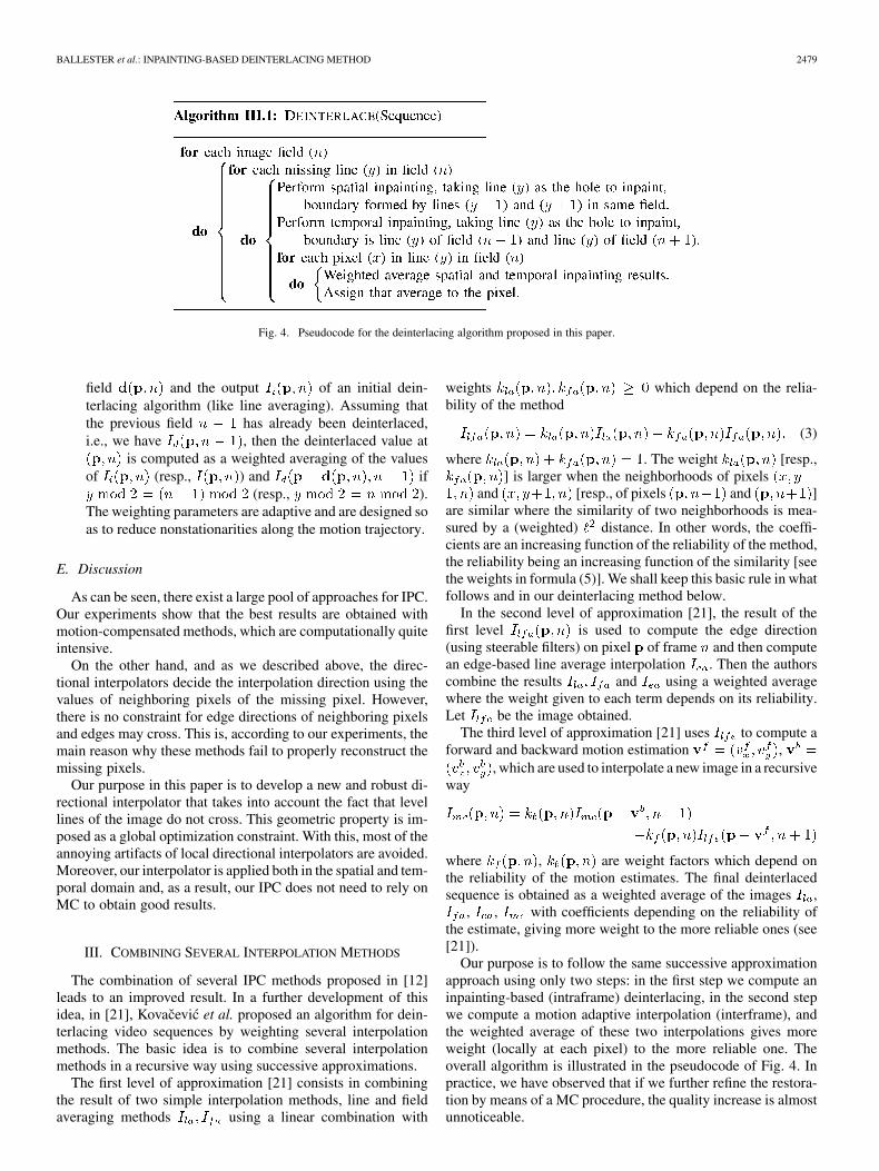
Our purpose is to follow the same successive approximationapproach using only two steps: in the first step we compute aninpainting-based (intraframe) deinterlacing, in the second stepwe compute a motion adaptive interpolation (interframe), andthe weighted average of these two interpolations gives moreweight (locally at each pixel) to the more reliable one. Theoverall algorithm is illustrated in the pseudocode of Fig. 4. Inpractice, we have observed that if we further refine the restora-tion by means of a MC procedure, the quality increase is almostunnoticeable.


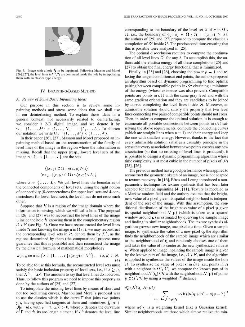
Fig. 5. Image with a hole H to be inpainted. Following Masnou and Morel[26], [27], the level lines innH are continued inside the hole by interpolatingthem with an elastica type energy.

IV. INPAINTING-BASED METHOD

A. Review of Some Basic Inpainting Ideas

Our purpose in this section is to review some in-painting methods and stress some ideas that we shall usein our deinterlacing method. To explain these ideas in ageneral context, not necessarily related to deinterlacing,we consider a 2-D digital image, and we denote it by

. To shortenour notation, we write .

In their paper [26], [27], Masnou and Morel proposed an in-painting method based on the reconstruction of the family oflevel lines of the image in the region where the information ismissing. Recall that the upper (resp., lower) level sets of theimage are the sets

where . We call level lines the boundaries ofthe connected components of level sets. Using the right notionof connectivity (8-connectedness for upper level sets and 4-con-nectedness for lower level sets), the level lines do not cross eachother.

Suppose that is a region of the image domain where theinformation is missing, which we will call a hole. The proposalin [26] and [27] was to reconstruct the level lines of the image

inside the hole knowing them in the complementary region(see Fig. 5). Once we have reconstructed the level lines

inside and knowing the image in , we may reconstructthe corresponding level sets in , denote them by , as theregions determined by them (the computational process mustguarantee that this is possible) and then reconstruct the imageby the classical formula of mathematical morphology

(4)To be able to use this formula, the reconstructed level sets mustsatisfy the basic inclusion property of level sets, i.e., if ,then . This amounts to say that level lines do not cross.Thus, to follow this program we need to impose this property asdone by the authors of [25] and [27].

To interpolate the missing level lines by means of short andnot too oscillating curves, Masnou and Morel’s proposal wasto use the elastica which is the curve that joins two points

having specified tangents at them and minimizes, with , , where denotes the curvature

of and its arc-length element. If denotes the level line

corresponding to the boundary of the level set of in, i.e., the boundary of ,

the authors of [25] and [27] proposed to compute the elastica’scompletion of inside . The precise conditions ensuring thatthis is possible were analyzed in [25].

The optimal disocclusion requires to compute the continua-tion of all level lines for any . To accomplish this, the au-thors add the elastica energy of all these completions [25] and[27] to obtain the final energy functional that is minimized.

Finally, in [25] and [26], choosing the power and re-laxing the tangent conditions at end points, the authors proposedan algorithm based on dynamic programming to find optimalpairing between compatible points in obtaining a minimumof the energy (whose existence was also proved). Compatiblepoints are points in with the same gray level and with thesame gradient orientation and they are candidates to be joinedby curves completing the level lines inside . Moreover, anadmissible solution should satisfy the property that two levellines connecting two pairs of compatible points should not cross.Then, in order to compute the optimal solution, it is enough toenumerate all possible connections between points in sat-isfying the above requirements, compute the connecting curves(which are straight lines when ) and their energy and keepthe one with smallest energy. However, thanks to the fact thatevery admissible solution satisfies a causality principle in thesense that every association between two points coerces any newassociation (so that no crossing of level lines is produced), itis possible to design a dynamic programming algorithm whosetime complexity is at most cubic in the number of pixels of[25], [26].

The previous method has a good performance when applied toreconstruct the geometric sketch of an image, but is not adaptedto texture recovery. In [16], Efros and Leung introduced a non-parametric technique for texture synthesis that has been lateradapted for image inpainting [4], [11]. Texture is modeled asa Markov random field and the authors assume that the bright-ness value of a pixel given its spatial neighborhood is indepen-dent of the rest of the image. With this assumption, the con-ditional distribution of the brightness value of a pixel givenits spatial neighborhood (which is taken as a squaredwindow around ) is estimated by querying the sample imageand finding its similar neighborhoods. The texture synthesis al-gorithm grows a new image, one pixel at a time. Given a sampleimage, to synthesize the value of a new pixel , the algorithmfinds the neighborhoods of the sample image which are similarto the neighborhood of and randomly chooses one of themand takes the value of its center as the new synthesized value at

. When applied to image inpainting the sample image is givenby the known part of the image, i.e., , and the algorithmis applied to synthesize the values of the image inside the hole

. To synthesize the value of pixel in (i.e., points inwith a neighbor in ), we compare the known part of itsneighborhood with the neighborhood of points

by using a weighted distance

where is a weighting kernel (like a Gaussian kernel).Similar neighborhoods are those which almost realize the min-


imum distance to and the distribution of its centervalues give a histogram for the values of which can thenrandomly sampled [16]. When a new pixel value is synthesizedthe hole is redefined by excluding this pixel. Initially, the orderof the pixels being synthesized was the standard concentriclayer filling, but this was improved in [11] by giving morepriority to pixels which are on the continuation of strong edgesand are surrounded by high-confidence pixels (they have largerknown parts in their neighborhoods), combining in such a waygeometry and texture inpainting. In both cases [11], [16], agreedy approach for hole filling is used. In [38], the authorsproposed a coherence measure to be optimized which tries tofind for each pixel to be reconstructed the most similar one(in terms of its neighborhood) in the sample image and theyapplied it to image and video completion. What is of interestto us here is that they proposed to compute the unknown pixelvalue by a weighted average of the values of pixels closeenough to in terms of

(5)

where the sum is extended to pixels with similar neighborhoodsto , the weight is a decreasingfunction of its argument expressing the reliability of thematching, the value of is chosen empirically dependingon the image noise, and is a normalization factor, i.e,

[38]. The paper in [28], whichwas pointed out to us by one of the reviewers, is devoted tofull-frame video stabilization using video completion and de-blurring algorithms and contains several interesting ideas thatcould have some application in the context of deinterlacing. Inparticular, if motion estimation (using neighboring frames) pro-duces a consistent estimate of a pixel value in a hole of a videosequence, then we can adopt it; otherwise, the authors proposeto use a technique based on motion inpainting combined withother spatial intraframe inpainting methods.

B. Inpainting-Based Method for Space Interpolation

We propose to combine the two main ideas described in Sec-tion IV-A for intraframe interpolation in an interlaced video se-quence . Given a fixed frame , let us consider twoconsecutive lines of the same parity and ,

, where the image is known and let us con-sider the unknown line , , as the hole tobe inpainted. We denote these lines by , , and , respec-tively. According to Masnou and Morel’s approach, since thelevel lines of the image do not cross, the connection of levellines between and , or, what amounts to the same, thereconstruction of the image in the missing line defines anondecreasing correspondence between points in and .On the other hand, due to the inclination of level lines and thepossible presence of an object in one line and not in the other, thecorrespondence is in general multivalued (see Fig. 6). Com-bining these two observations, we define as a nondecreasingmultivalued map, that is, a map which assigns to eachan interval and such that:

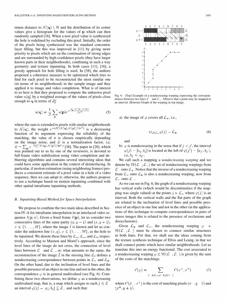
Fig. 6. (Top) Example of a nondecreasing warping expressing the correspon-dences between two lines L and L . Observe that a point may be mapped toan interval. (Bottom) Graph of the warping in top image.

a) the image of covers all , i.e.,

(6)

andb) is nondecreasing in the sense that if , the interval

is located at the left of ,i.e, .

We call such a mapping a nondecreasing warping and wedenote by the set of nondecreasing warpings from

onto . Notice that the inverse of a nondecreasing warpingfrom onto is also a nondecreasing warping, now from

onto .As we can see in Fig. 6, the graph of a nondecreasing warping

has vertical walls (which would be discontinuities if the map-ping was single valued) at the points where is aninterval. Both the vertical walls and the flat parts of the graphare related to the inclination of level lines and possible pres-ence of an object in one line and not in the other (in the applica-tions of this technique to compute correspondences in pairs ofstereo images this is related to the presence of occlusions anddisocclusions).

Given and , the nondecreasing warpingmust be chosen to connect similar structures

in both lines. For that, we shall use the ideas coming fromthe texture synthesis technique of Efros and Leung, in that weshall connect points which have similar neighborhoods. Let ustranslate this into an energy functional. The cost associated toa nondecreasing warping is given by the sumof the costs of the matchings

(7)

where is the cost of matching pixels and.


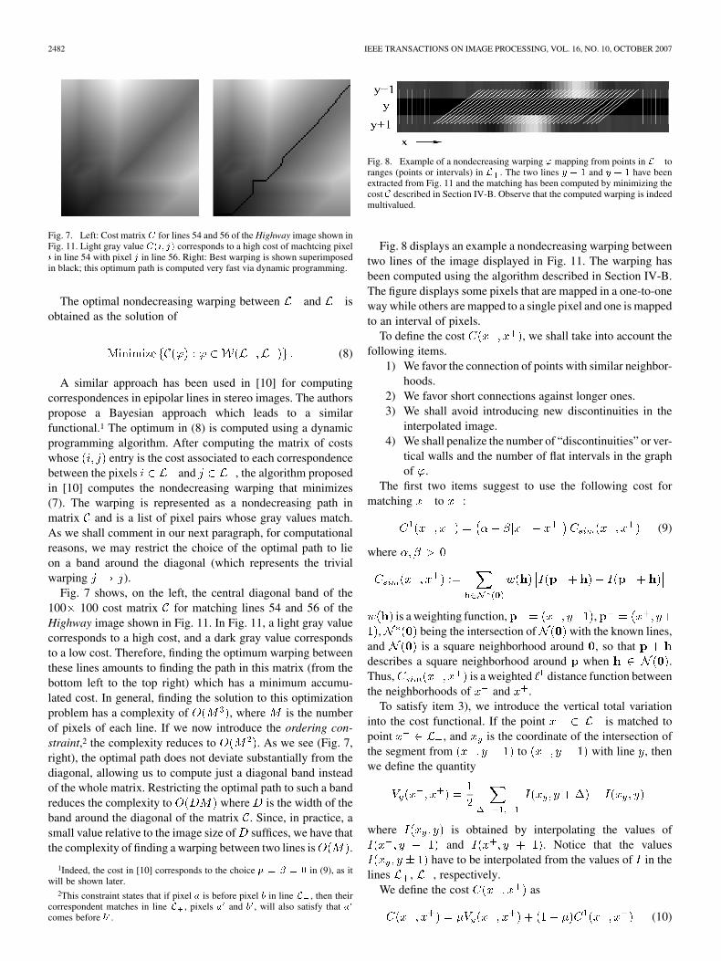
Fig. 7. Left: Cost matrix C for lines 54 and 56 of the Highway image shown inFig. 11. Light gray value C(i; j) corresponds to a high cost of machtcing pixeli in line 54 with pixel j in line 56. Right: Best warping is shown superimposedin black; this optimum path is computed very fast via dynamic programming.

The optimal nondecreasing warping between and isobtained as the solution of

(8)

A similar approach has been used in [10] for computingcorrespondences in epipolar lines in stereo images. The authorspropose a Bayesian approach which leads to a similarfunctional.1 The optimum in (8) is computed using a dynamicprogramming algorithm. After computing the matrix of costswhose entry is the cost associated to each correspondencebetween the pixels and , the algorithm proposedin [10] computes the nondecreasing warping that minimizes(7). The warping is represented as a nondecreasing path inmatrix and is a list of pixel pairs whose gray values match.As we shall comment in our next paragraph, for computationalreasons, we may restrict the choice of the optimal path to lieon a band around the diagonal (which represents the trivialwarping ).

Fig. 7 shows, on the left, the central diagonal band of the100 100 cost matrix for matching lines 54 and 56 of theHighway image shown in Fig. 11. In Fig. 11, a light gray valuecorresponds to a high cost, and a dark gray value correspondsto a low cost. Therefore, finding the optimum warping betweenthese lines amounts to finding the path in this matrix (from thebottom left to the top right) which has a minimum accumu-lated cost. In general, finding the solution to this optimizationproblem has a complexity of , where is the numberof pixels of each line. If we now introduce the ordering con-straint,2 the complexity reduces to . As we see (Fig. 7,right), the optimal path does not deviate substantially from thediagonal, allowing us to compute just a diagonal band insteadof the whole matrix. Restricting the optimal path to such a bandreduces the complexity to where is the width of theband around the diagonal of the matrix . Since, in practice, asmall value relative to the image size of suffices, we have thatthe complexity of finding a warping between two lines is .

1Indeed, the cost in [10] corresponds to the choice � = � = 0 in (9), as itwill be shown later.

2This constraint states that if pixel a is before pixel b in line L , then theircorrespondent matches in line L , pixels a and b , will also satisfy that acomes before b .

Fig. 8. Example of a nondecreasing warping ' mapping from points in L toranges (points or intervals) in L . The two lines y � 1 and y + 1 have beenextracted from Fig. 11 and the matching has been computed by minimizing thecost C described in Section IV-B. Observe that the computed warping is indeedmultivalued.

Fig. 8 displays an example a nondecreasing warping betweentwo lines of the image displayed in Fig. 11. The warping hasbeen computed using the algorithm described in Section IV-B.The figure displays some pixels that are mapped in a one-to-oneway while others are mapped to a single pixel and one is mappedto an interval of pixels.

To define the cost , we shall take into account thefollowing items.

1) We favor the connection of points with similar neighbor-hoods.

2) We favor short connections against longer ones.3) We shall avoid introducing new discontinuities in the

interpolated image.4) We shall penalize the number of “discontinuities” or ver-

tical walls and the number of flat intervals in the graphof .

The first two items suggest to use the following cost formatching to :

(9)

where

is a weighting function, ,, being the intersection of with the known lines,

and is a square neighborhood around , so thatdescribes a square neighborhood around when .Thus, is a weighted distance function betweenthe neighborhoods of and .

To satisfy item 3), we introduce the vertical total variationinto the cost functional. If the point is matched topoint , and is the coordinate of the intersection ofthe segment from to with line , thenwe define the quantity

where is obtained by interpolating the values ofand . Notice that the values

have to be interpolated from the values of in thelines , , respectively.

We define the cost as

(10)


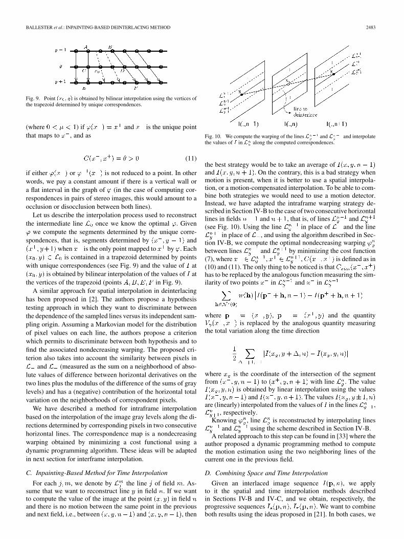
Fig. 9. Point (x ; y) is obtained by bilinear interpolation using the vertices ofthe trapezoid determined by unique correspondences.

(where ) if and is the unique pointthat maps to , and as

(11)

if either or is not reduced to a point. In otherwords, we pay a constant amount if there is a vertical wall ora flat interval in the graph of (in the case of computing cor-respondences in pairs of stereo images, this would amount to aocclusion or disocclusion between both lines).

Let us describe the interpolation process used to reconstructthe intermediate line once we know the optimal . Given

we compute the segments determined by the unique corre-spondences, that is, segments determined by and

when is the only point mapped to by . Eachis contained in a trapezoid determined by points

with unique correspondences (see Fig. 9) and the value of atis obtained by bilinear interpolation of the values of at

the vertices of the trapezoid (points in Fig. 9).A similar approach for spatial interpolation in deinterlacing

has been proposed in [2]. The authors propose a hypothesistesting approach in which they want to discriminate betweenthe dependence of the sampled lines versus its independent sam-pling origin. Assuming a Markovian model for the distributionof pixel values on each line, the authors propose a criterionwhich permits to discriminate between both hypothesis and tofind the associated nondecreasing warping. The proposed cri-terion also takes into account the similarity between pixels in

and (measured as the sum on a neighborhood of abso-lute values of difference between horizontal derivatives on thetwo lines plus the modulus of the difference of the sums of graylevels) and has a (negative) contribution of the horizontal totalvariation on the neighborhoods of correspondent pixels.

We have described a method for intraframe interpolationbased on the interpolation of the image gray levels along the di-rections determined by corresponding pixels in two consecutivehorizontal lines. The correspondence map is a nondecreasingwarping obtained by minimizing a cost functional using adynamic programming algorithm. These ideas will be adaptedin next section for interframe interpolation.

C. Inpainting-Based Method for Time Interpolation

For each , we denote by the line of field . As-sume that we want to reconstruct line in field . If we wantto compute the value of the image at the point in fieldand there is no motion between the same point in the previousand next field, i.e., between and , then

Fig. 10. We compute the warping of the lines L and L and interpolatethe values of I in L along the computed correspondences.

the best strategy would be to take an average ofand . On the contrary, this is a bad strategy whenmotion is present, when it is better to use a spatial interpola-tion, or a motion-compensated interpolation. To be able to com-bine both strategies we would need to use a motion detector.Instead, we have adapted the intraframe warping strategy de-scribed in Section IV-B to the case of two consecutive horizontallines in fields and , that is, of lines and(see Fig. 10). Using the line in place of and the line

in place of , and using the algorithm described in Sec-tion IV-B, we compute the optimal nondecreasing warpingbetween lines and by minimizing the cost function(7), where , , is defined as in(10) and (11). The only thing to be noticed is thathas to be replaced by the analogous function measuring the sim-ilarity of two points in and in

where , and the quantityis replaced by the analogous quantity measuring

the total variation along the time direction

where is the coordinate of the intersection of the segmentfrom to with line . The value

is obtained by linear interpolation using the valuesand . The values

are (linearly) interpolated from the values of in the lines ,, respectively.

Knowing , line is reconstructed by interpolating linesand using the scheme described in Section IV-B.

A related approach to this step can be found in [33] where theauthor proposed a dynamic programming method to computethe motion estimation using the two neighboring lines of thecurrent one in the previous field.

D. Combining Space and Time Interpolation

Given an interlaced image sequence , we applyto it the spatial and time interpolation methods describedin Sections IV-B and IV-C, and we obtain, respectively, theprogressive sequences , . We want to combineboth results using the ideas proposed in [21]. In both cases, we


minimize the same functional, applied to two consecutive linesof the same frame in case of spatial interpolation and to thelines and in the case of time interpolation. Let usdenote the cost defined by (10) and (11) by in case of thespatial interpolation and by in the case of time interpolation.

Now, let us consider a line which was missing in theoriginal interlaced sequence and has been reconstructed in bothimages , . As described in Section III, we cancombine both results , by linear combinationwith coefficients which are functions of a reliability measurecomputed for each of them. We define the reliability as a de-creasing function of the cost, so that lower cost implies higherreliability, concretely, we use

(12)

where is a point on the line . Then we combine, using the formula

(13)

We have also experimented with another choice of weights.When computing the coefficients , instead of considering justthe value of the cost ( or ) at pixel , we average the coston a neighborhood of , so we get

where is a positive integer. If , our weights aredefined as

(14)

and if , they are defined as

(15)

where . Experimentally, the deinterlacing results obtainedusing the weights defined in (12) or those in (14) and (15) arealmost identical in terms of mean square error (MSE), thoughwe have observed that the second choice of coefficients mayyield less visual artifacts in some video sequences.

These formulas are similar in spirit to those used in [21],though different in form. They are similar to those used in [38],where the authors observed that is the value of thatminimizes the quantity

Let us comment on a technical point. Notice that the coeffi-cients , in (12) and (13) are defined on points

on the line . However, originally, the costs ,

were not defined on those points. Let us explain how tocompute on points in , the case of being anal-ogous. With that purpose, let be the optimal nondecreasingwarping between and obtained for the space (in-traframe) interpolation of . As explained in Section IV-B,recall that each point is contained in atrapezoid determined by points with unique correspondences(see Fig. 9). Referring to Fig. 9, point is contained inthe trapezoid determined by the correspondencesand . Since is in the segment determined by

and , we have that for some. Then we define the cost by linear interpo-

lation of the costs of the correspondences to and to ,that is, . In a similarway, we define .

V. EXPERIMENTAL RESULTS

In this section, we will discuss the results that are obtainedwith the proposed method.

Our dynamic programming implementation is inspired by theone proposed by Cox et al. for stereo matching [10]. It is writtenin C++ under Linux running on a Dual-core 3-GHz 2-Gb PC.The per-frame complexity is where is thenumber of image pixels. For a frame of TV dimensions (640480) the total processing time per frame is roughly 1.3 s. Thismay seem rather too much time given the low complexity ofthe algorithm, but the bottleneck lies not in the CPU processingtime but rather in the data-bus transfer rate. Please bear in mindthat for each line in each frame field we have to createtwo floating-point matrices (for and ) and twounsigned char matrices (for backtracking in computing the op-timal path,) which in the case of TV resolution and using 4 bytesper floating-point number, imply the need to transfer betweenmemory and the CPU an amount of

GB per frame, while typical data-bus transfer rates rangefrom 1.5 to 8 GB/s. Of course, if for each matrix, we only com-pute a diagonal band, the speed increase is considerable, butwe are still far from deinterlacing at a rate of 25–30 frames persecond. We are currently exploring GPU acceleration in orderto bring our algorithm down to real time: see, for instance, [18]and [24], where they use programmable graphics hardware tosolve problems which in essence are quite similar to IPC.

All of our tests have been executed using the same set of pa-rameters. is a neighborhood of 5 3 pixels,

where is the cardinality of the setand is the intersection of with the known lines.In our case, . We do not observe significantdifferences in the results if we vary the size of between5 3 and 9 5. For , we have used , .Actually, given the way these parameters appear in the compu-tation of the cost matrix [see (9)], it is only their ratio what weshould take into account, i.e., we may consider as a parameterjust . We have tested several values of this ratio, in the range5.7–19.0, with no significant change in the MSE of the results.For [see (10)], we have chosen . We have observedthat if we decrease the value of this parameter the results remainalmost unchanged when we use the choice of weights presented


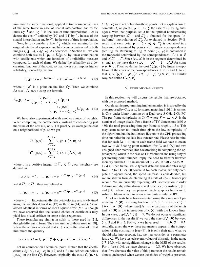
Fig. 11. Example of IPC applying the geometrical-based approach. Left: Inter-laced image. Right: IPC reconstructed image obtained with our proposed spatialreconstruction approach.

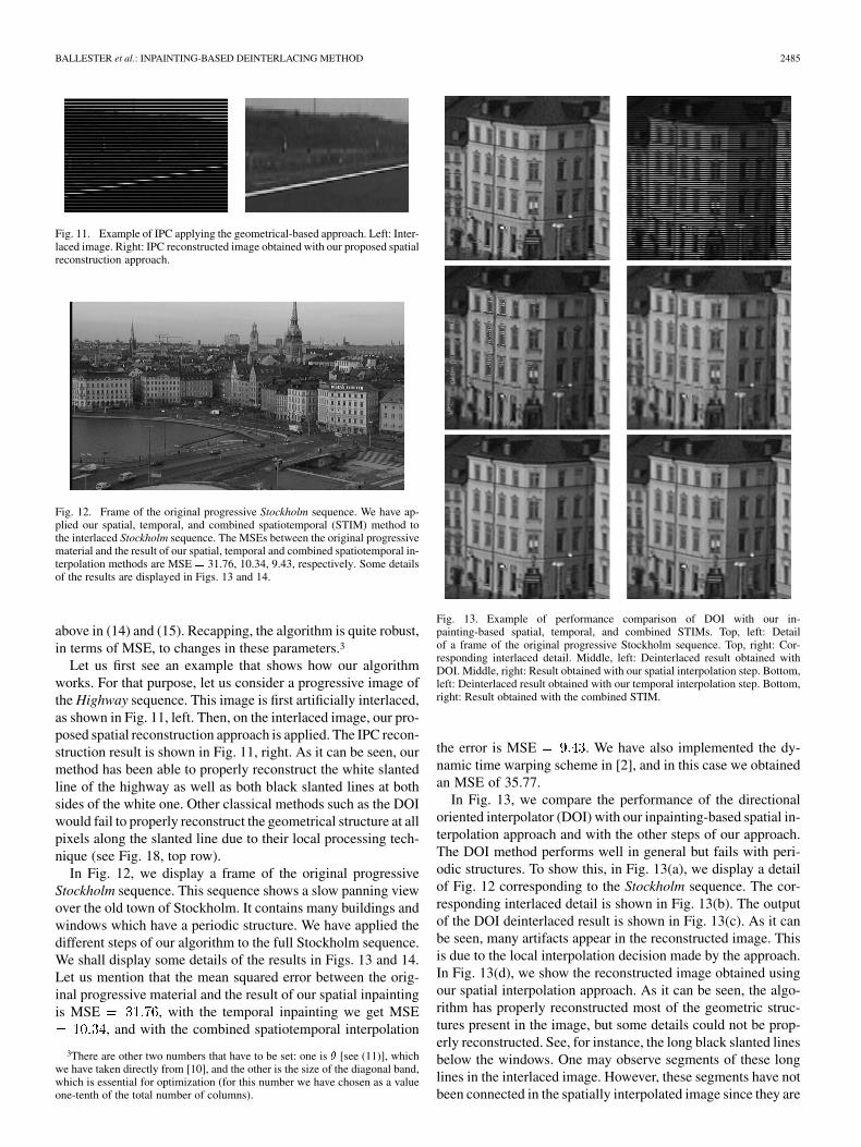
Fig. 12. Frame of the original progressive Stockholm sequence. We have ap-plied our spatial, temporal, and combined spatiotemporal (STIM) method tothe interlaced Stockholm sequence. The MSEs between the original progressivematerial and the result of our spatial, temporal and combined spatiotemporal in-terpolation methods are MSE = 31.76, 10.34, 9.43, respectively. Some detailsof the results are displayed in Figs. 13 and 14.

above in (14) and (15). Recapping, the algorithm is quite robust,in terms of MSE, to changes in these parameters.3

Let us first see an example that shows how our algorithmworks. For that purpose, let us consider a progressive image ofthe Highway sequence. This image is first artificially interlaced,as shown in Fig. 11, left. Then, on the interlaced image, our pro-posed spatial reconstruction approach is applied. The IPC recon-struction result is shown in Fig. 11, right. As it can be seen, ourmethod has been able to properly reconstruct the white slantedline of the highway as well as both black slanted lines at bothsides of the white one. Other classical methods such as the DOIwould fail to properly reconstruct the geometrical structure at allpixels along the slanted line due to their local processing tech-nique (see Fig. 18, top row).

In Fig. 12, we display a frame of the original progressiveStockholm sequence. This sequence shows a slow panning viewover the old town of Stockholm. It contains many buildings andwindows which have a periodic structure. We have applied thedifferent steps of our algorithm to the full Stockholm sequence.We shall display some details of the results in Figs. 13 and 14.Let us mention that the mean squared error between the orig-inal progressive material and the result of our spatial inpaintingis MSE , with the temporal inpainting we get MSE

, and with the combined spatiotemporal interpolation

3There are other two numbers that have to be set: one is � [see (11)], whichwe have taken directly from [10], and the other is the size of the diagonal band,which is essential for optimization (for this number we have chosen as a valueone-tenth of the total number of columns).

Fig. 13. Example of performance comparison of DOI with our in-painting-based spatial, temporal, and combined STIMs. Top, left: Detailof a frame of the original progressive Stockholm sequence. Top, right: Cor-responding interlaced detail. Middle, left: Deinterlaced result obtained withDOI. Middle, right: Result obtained with our spatial interpolation step. Bottom,left: Deinterlaced result obtained with our temporal interpolation step. Bottom,right: Result obtained with the combined STIM.

the error is MSE . We have also implemented the dy-namic time warping scheme in [2], and in this case we obtainedan MSE of 35.77.

In Fig. 13, we compare the performance of the directionaloriented interpolator (DOI) with our inpainting-based spatial in-terpolation approach and with the other steps of our approach.The DOI method performs well in general but fails with peri-odic structures. To show this, in Fig. 13(a), we display a detailof Fig. 12 corresponding to the Stockholm sequence. The cor-responding interlaced detail is shown in Fig. 13(b). The outputof the DOI deinterlaced result is shown in Fig. 13(c). As it canbe seen, many artifacts appear in the reconstructed image. Thisis due to the local interpolation decision made by the approach.In Fig. 13(d), we show the reconstructed image obtained usingour spatial interpolation approach. As it can be seen, the algo-rithm has properly reconstructed most of the geometric struc-tures present in the image, but some details could not be prop-erly reconstructed. See, for instance, the long black slanted linesbelow the windows. One may observe segments of these longlines in the interlaced image. However, these segments have notbeen connected in the spatially interpolated image since they are


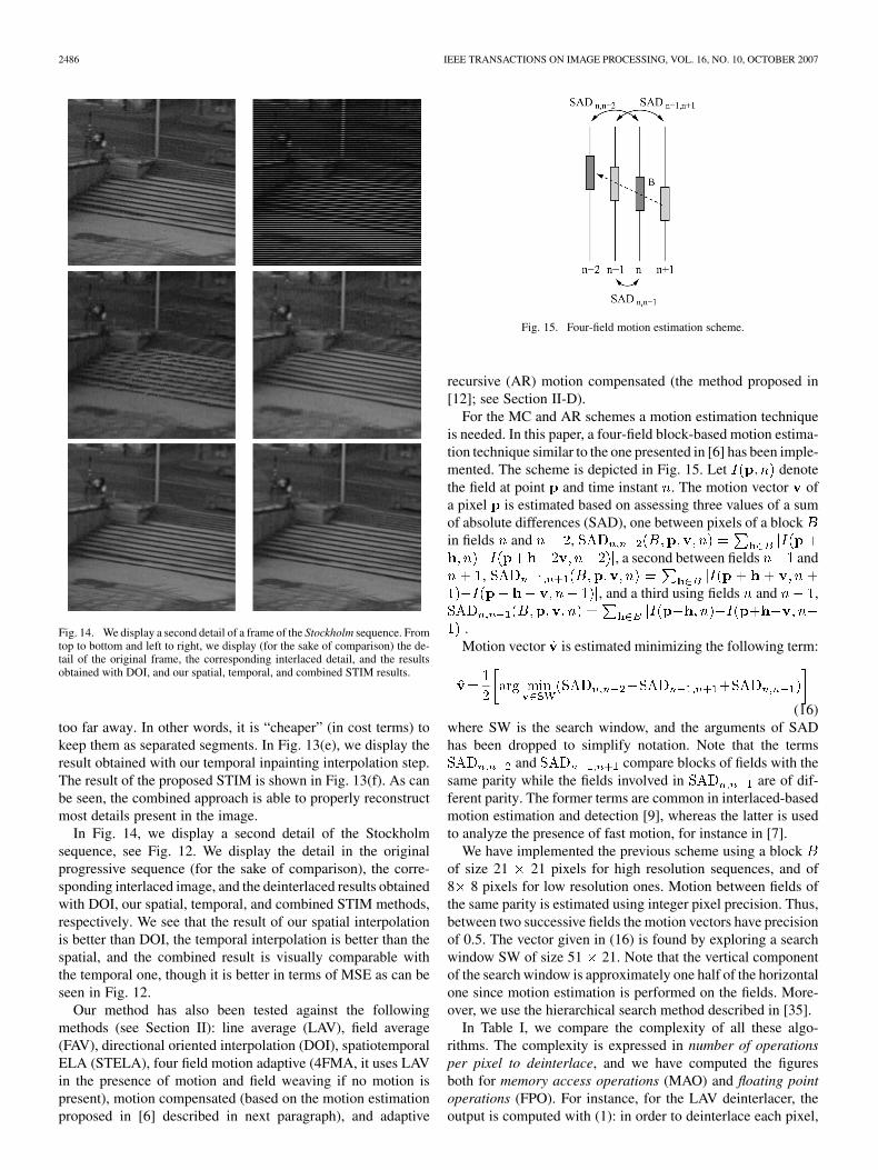
Fig. 14. We display a second detail of a frame of the Stockholm sequence. Fromtop to bottom and left to right, we display (for the sake of comparison) the de-tail of the original frame, the corresponding interlaced detail, and the resultsobtained with DOI, and our spatial, temporal, and combined STIM results.

too far away. In other words, it is “cheaper” (in cost terms) tokeep them as separated segments. In Fig. 13(e), we display theresult obtained with our temporal inpainting interpolation step.The result of the proposed STIM is shown in Fig. 13(f). As canbe seen, the combined approach is able to properly reconstructmost details present in the image.

In Fig. 14, we display a second detail of the Stockholmsequence, see Fig. 12. We display the detail in the originalprogressive sequence (for the sake of comparison), the corre-sponding interlaced image, and the deinterlaced results obtainedwith DOI, our spatial, temporal, and combined STIM methods,respectively. We see that the result of our spatial interpolationis better than DOI, the temporal interpolation is better than thespatial, and the combined result is visually comparable withthe temporal one, though it is better in terms of MSE as can beseen in Fig. 12.

Our method has also been tested against the followingmethods (see Section II): line average (LAV), field average(FAV), directional oriented interpolation (DOI), spatiotemporalELA (STELA), four field motion adaptive (4FMA, it uses LAVin the presence of motion and field weaving if no motion ispresent), motion compensated (based on the motion estimationproposed in [6] described in next paragraph), and adaptive

Fig. 15. Four-field motion estimation scheme.

recursive (AR) motion compensated (the method proposed in[12]; see Section II-D).

For the MC and AR schemes a motion estimation techniqueis needed. In this paper, a four-field block-based motion estima-tion technique similar to the one presented in [6] has been imple-mented. The scheme is depicted in Fig. 15. Let denotethe field at point and time instant . The motion vector ofa pixel is estimated based on assessing three values of a sumof absolute differences (SAD), one between pixels of a blockin fields and ,

, a second between fields and,

, and a third using fields and ,

.Motion vector is estimated minimizing the following term:

(16)where SW is the search window, and the arguments of SADhas been dropped to simplify notation. Note that the terms

and compare blocks of fields with thesame parity while the fields involved in are of dif-ferent parity. The former terms are common in interlaced-basedmotion estimation and detection [9], whereas the latter is usedto analyze the presence of fast motion, for instance in [7].

We have implemented the previous scheme using a blockof size 21 21 pixels for high resolution sequences, and of8 8 pixels for low resolution ones. Motion between fields ofthe same parity is estimated using integer pixel precision. Thus,between two successive fields the motion vectors have precisionof 0.5. The vector given in (16) is found by exploring a searchwindow SW of size 51 21. Note that the vertical componentof the search window is approximately one half of the horizontalone since motion estimation is performed on the fields. More-over, we use the hierarchical search method described in [35].

In Table I, we compare the complexity of all these algo-rithms. The complexity is expressed in number of operationsper pixel to deinterlace, and we have computed the figuresboth for memory access operations (MAO) and floating pointoperations (FPO). For instance, for the LAV deinterlacer, theoutput is computed with (1): in order to deinterlace each pixel,


TABLE IMAO (MEMORY ACCESS OPERATIONS) AND FPO (FLOATING POINT

OPERATIONS) PER PIXEL, FOR SEVERAL DEINTERLACING

METHODS. SEE TEXT FOR DETAILS

a sum and a division are performed (requiring two FPO) andtwo pixel accesses are needed (requiring two MAO), plus oneMAO in order to store the result in the corresponding pixelposition (3 MAO in total). Four our proposed STIM algorithmwe show the figures for two different choices of the width

of the diagonal band used in the computation of the costmatrix: 21, 41. For the MC scheme we show the figuresfor two choices of a multiscale implementation: just one level

, and three levels . We must stress that theMC technique is block-based, with blocks of size 21 21pixels, i.e., we compute one vector per 21 21 block, whereasin STIM matches are computed per-pixel and not per-block.Despite this fact, STIM (with ) needs roughly one fifthof the operations required by the one-level implementation ofthe MC scheme, and has approximately half the complexity ofthe three-level implementation of the MC scheme.

Several different test sequences have been employed, three ofthem are of CIF dimensions (352 288) while the other four areof high resolution (1280 720). In Fig. 18(a), the key frame ofeach sequence is shown on the left column. We include a briefdescription of them here.

• Mobile (352 288): The Mobile & Calendar sequence.The camera pans left following the movement of an elec-tric train, with a calendar moving vertically behind it. Inthe background there is a wallpaper with several figures.Frames 0 to 29 have been used.

• Paris (352 288): A man and a woman moving in frontof a detailed static background. Frames 0 to 29 have beenused.

• Highway (352 288): View from inside a car travelingalong a highway. Features some fast moving objects andslanted lines with different slopes. Used frames 0 to 29.

• Stockholm (1280 720): Slow pan over a city landscape.Lots of detail and structue. Frames 100 to 129 have beenused for the tests.

• Parkrun (1280 720): Slow lateral dolly of a man runningin a park. Many details and different textures. Used frames20 to 49.

• Train (1280 720): A calendar with text moves verti-cally, a toy train moves horizontally. Different textures andprinted figures. Used frames 460 to 489.

• Shields (1280 720): A man points to a wall with differentshields. Used frames 440 to 469 since it contains a slowzoom-in.

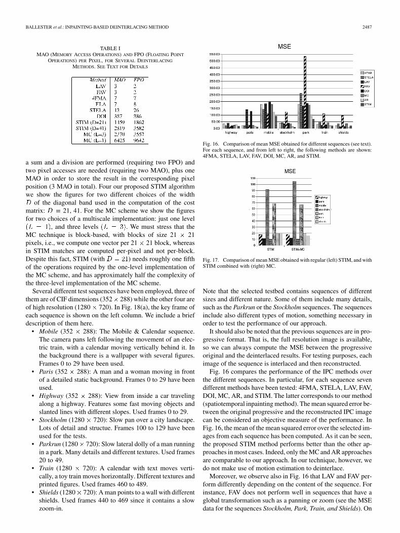
Fig. 16. Comparison of mean MSE obtained for different sequences (see text).For each sequence, and from left to right, the following methods are shown:4FMA, STELA, LAV, FAV, DOI, MC, AR, and STIM.

Fig. 17. Comparison of mean MSE obtained with regular (left) STIM, and withSTIM combined with (right) MC.

Note that the selected testbed contains sequences of differentsizes and different nature. Some of them include many details,such as the Parkrun or the Stockholm sequences. The sequencesinclude also different types of motion, something necessary inorder to test the performance of our approach.

It should also be noted that the previous sequences are in pro-gressive format. That is, the full resolution image is available,so we can always compute the MSE between the progressiveoriginal and the deinterlaced results. For testing purposes, eachimage of the sequence is interlaced and then reconstructed.

Fig. 16 compares the performance of the IPC methods overthe different sequences. In particular, for each sequence sevendifferent methods have been tested: 4FMA, STELA, LAV, FAV,DOI, MC, AR, and STIM. The latter corresponds to our method(spatiotemporal inpainting method). The mean squared error be-tween the original progressive and the reconstructed IPC imagecan be considered an objective measure of the performance. InFig. 16, the mean of the mean squared error over the selected im-ages from each sequence has been computed. As it can be seen,the proposed STIM method performs better than the other ap-proaches in most cases. Indeed, only the MC and AR approachesare comparable to our approach. In our technique, however, wedo not make use of motion estimation to deinterlace.

Moreover, we observe also in Fig. 16 that LAV and FAV per-form differently depending on the content of the sequence. Forinstance, FAV does not perform well in sequences that have aglobal transformation such as a panning or zoom (see the MSEdata for the sequences Stockholm, Park, Train, and Shields). On


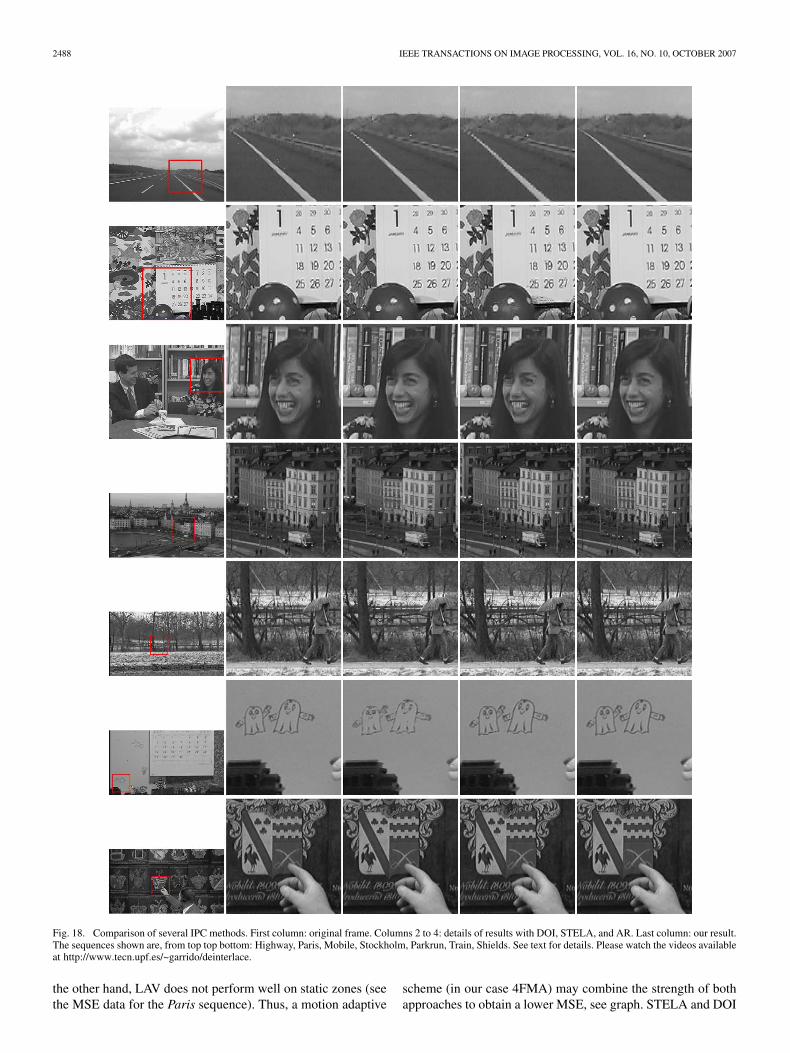
Fig. 18. Comparison of several IPC methods. First column: original frame. Columns 2 to 4: details of results with DOI, STELA, and AR. Last column: our result.The sequences shown are, from top top bottom: Highway, Paris, Mobile, Stockholm, Parkrun, Train, Shields. See text for details. Please watch the videos availableat http://www.tecn.upf.es/~garrido/deinterlace.

the other hand, LAV does not perform well on static zones (seethe MSE data for the Paris sequence). Thus, a motion adaptive

scheme (in our case 4FMA) may combine the strength of bothapproaches to obtain a lower MSE, see graph. STELA and DOI


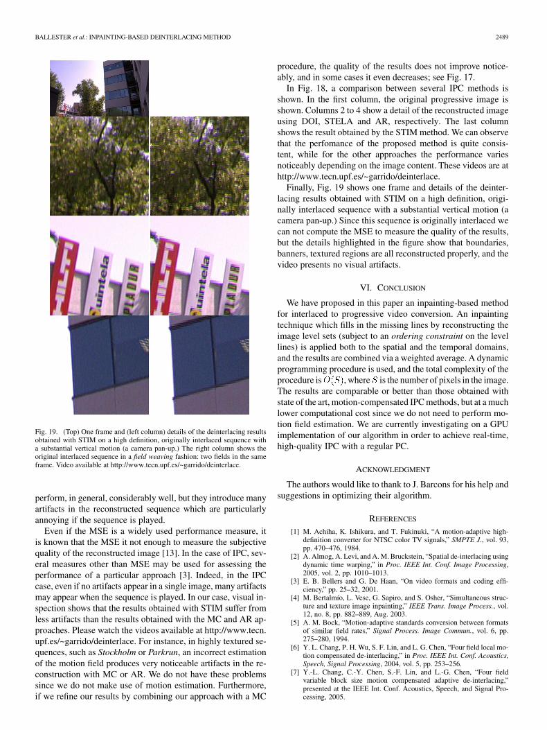
Fig. 19. (Top) One frame and (left column) details of the deinterlacing resultsobtained with STIM on a high definition, originally interlaced sequence witha substantial vertical motion (a camera pan-up.) The right column shows theoriginal interlaced sequence in a field weaving fashion: two fields in the sameframe. Video available at http://www.tecn.upf.es/~garrido/deinterlace.

perform, in general, considerably well, but they introduce manyartifacts in the reconstructed sequence which are particularlyannoying if the sequence is played.

Even if the MSE is a widely used performance measure, itis known that the MSE it not enough to measure the subjectivequality of the reconstructed image [13]. In the case of IPC, sev-eral measures other than MSE may be used for assessing theperformance of a particular approach [3]. Indeed, in the IPCcase, even if no artifacts appear in a single image, many artifactsmay appear when the sequence is played. In our case, visual in-spection shows that the results obtained with STIM suffer fromless artifacts than the results obtained with the MC and AR ap-proaches. Please watch the videos available at http://www.tecn.upf.es/~garrido/deinterlace. For instance, in highly textured se-quences, such as Stockholm or Parkrun, an incorrect estimationof the motion field produces very noticeable artifacts in the re-construction with MC or AR. We do not have these problemssince we do not make use of motion estimation. Furthermore,if we refine our results by combining our approach with a MC

procedure, the quality of the results does not improve notice-ably, and in some cases it even decreases; see Fig. 17.

In Fig. 18, a comparison between several IPC methods isshown. In the first column, the original progressive image isshown. Columns 2 to 4 show a detail of the reconstructed imageusing DOI, STELA and AR, respectively. The last columnshows the result obtained by the STIM method. We can observethat the perfomance of the proposed method is quite consis-tent, while for the other approaches the performance variesnoticeably depending on the image content. These videos are athttp://www.tecn.upf.es/~garrido/deinterlace.

Finally, Fig. 19 shows one frame and details of the deinter-lacing results obtained with STIM on a high definition, origi-nally interlaced sequence with a substantial vertical motion (acamera pan-up.) Since this sequence is originally interlaced wecan not compute the MSE to measure the quality of the results,but the details highlighted in the figure show that boundaries,banners, textured regions are all reconstructed properly, and thevideo presents no visual artifacts.

VI. CONCLUSION

We have proposed in this paper an inpainting-based methodfor interlaced to progressive video conversion. An inpaintingtechnique which fills in the missing lines by reconstructing theimage level sets (subject to an ordering constraint on the levellines) is applied both to the spatial and the temporal domains,and the results are combined via a weighted average. A dynamicprogramming procedure is used, and the total complexity of theprocedure is , where is the number of pixels in the image.The results are comparable or better than those obtained withstate of the art, motion-compensated IPC methods, but at a muchlower computational cost since we do not need to perform mo-tion field estimation. We are currently investigating on a GPUimplementation of our algorithm in order to achieve real-time,high-quality IPC with a regular PC.

ACKNOWLEDGMENT

The authors would like to thank to J. Barcons for his help andsuggestions in optimizing their algorithm.

REFERENCES

[1] M. Achiha, K. Ishikura, and T. Fukinuki, “A motion-adaptive high-definition converter for NTSC color TV signals,” SMPTE J., vol. 93,pp. 470–476, 1984.

[2] A. Almog, A. Levi, and A. M. Bruckstein, “Spatial de-interlacing usingdynamic time warping,” in Proc. IEEE Int. Conf. Image Processing,2005, vol. 2, pp. 1010–1013.

[3] E. B. Bellers and G. De Haan, “On video formats and coding effi-ciency,” pp. 25–32, 2001.

[4] M. Bertalmío, L. Vese, G. Sapiro, and S. Osher, “Simultaneous struc-ture and texture image inpainting,” IEEE Trans. Image Process., vol.12, no. 8, pp. 882–889, Aug. 2003.

[5] A. M. Bock, “Motion-adaptive standards conversion between formatsof similar field rates,” Signal Process. Image Commun., vol. 6, pp.275–280, 1994.

[6] Y. L. Chang, P. H. Wu, S. F. Lin, and L. G. Chen, “Four field local mo-tion compensated de-interlacing,” in Proc. IEEE Int. Conf. Acoustics,Speech, Signal Processing, 2004, vol. 5, pp. 253–256.

[7] Y.-L. Chang, C.-Y. Chen, S.-F. Lin, and L.-G. Chen, “Four fieldvariable block size motion compensated adaptive de-interlacing,”presented at the IEEE Int. Conf. Acoustics, Speech, and Signal Pro-cessing, 2005.


[8] M. J. Chen, C. H. Huang, and C. T. Hsu, “Efficient de-interlacing tech-nique by inter-field information,” IEEE Trans. Consum. Electron., vol.50, no. 4, pp. 1202–1208, Nov. 2004.

[9] C. Ciuhu and G. de Haan, “Motion estimation on interlaced video,”Proc. SPIE, vol. 5685, pp. 718–729, 2005.

[10] I. J. Cox, S. L. Hingorani, S. B. Rao, and B. M. Maggs, “A maximumlikelihood stereo algorithm,” Comput. Vis. Image Understand., vol. 63,no. 3, pp. 542–567, 1996.

[11] A. Criminisi, P. Perez, and K. Toyama, “Region filling and objectremoval by exemplar-based image inpainting,” IEEE Trans. ImageProcess., vol. 13, no. 9, pp. 1200–1212, Sep. 2004.

[12] G. De Haan and E. B. Bellers, “De-interlacing of video data,” IEEETrans. Consum. Electron., vol. 43, no. 8, pp. 819–825, Aug. 1997.

[13] G. De Haan and E. B. Bellers, “Deinterlacing—An overview,” Proc.IEEE, vol. 86, no. 9, pp. 1839–1857, Sep. 1998.

[14] T. Doyle, “Interlaced to sequential conversion for EDTV applications,”in Proc. 2nd. Int. Workshop Signal Processing of HDTV, 1988, pp.412–430.

[15] T. Doyle and M. Looymans, “Progressive scan conversion using edgeinformation,” in Proc. Signal Processing HDTV II, 1990, pp. 711–721.

[16] A. A. Efros and T. K. Leung, “Texture synthesis by non-parametricsampling,” in Proc. ICCV, 1999, vol. 2, pp. 1033–1038.

[17] P. D. Filliman, T. J. Christopher, and R. T. Keen, “Interlace to progres-sive scan converter for IDTV,” IEEE Trans. Consum. Electron., vol. 38,no. 8, pp. 135–144, Aug. 1992.

[18] M. Gong and Y. G. Yang, “Near real-time reliable stereo matchingusing programmable graphics hardware,” in Proc. IEEE Computer So-ciety Conf. Computer Vision and Pattern Recognition, Jun. 2005, vol.1, pp. 924–931.

[19] P. Haavisto, J. Juhola, and Y. Neuvo, “Scan rate-up conversion usingadaptive weighted median filtering,” in Proc. Signal Processing ofHDTV II, 1990, pp. 703–710.

[20] Y. Kim and Y. Cho, “Motion adaptive deinterlacing algorithm basedon wide vector correlations and edge dependent motion switching,” inProc. HDTV Workshop, 1995, pp. 8B9–8B16.

[21] J. Kovacevic, R. J. Safranek, and E. M. Yeh, “Deinterlacing by suc-cessive approximation,” IEEE Trans. Image Process., vol. 6, no. 2, pp.339–344, Feb. 1997.

[22] C. L. Lee, S. Chang, and C. W. Jen, “Motion detection and motionadaptive pro-scan conversion,” in Proc. IEEE Int. Symp. Circuits andSystems, Jun. 1991, vol. 1, pp. 666–669.

[23] M. Lee, J. Kim, J. Lee, K. Ryu, and D. Song, “A new algorithm forinterlaced to progressive scan conversion based on directional correla-tions and its ic design,” IEEE Trans. Consum. Electron., vol. 40, no. 5,pp. 119–129, May 1994.

[24] W. Liu, B. Schmidt, G. Voss, A. Schroder, and W. Muller-Wittig, “Bio-sequence database scanning on a gpu,” in Proc. 20th Int. Parallel andDistributed Processing Symp., Apr. 2006, pp. 1–8.

[25] S. Masnou, “Filtrage et desocclusion d’images par méthodes d’en-sembles de Niveau,” Ph.D. dissertation, Univ. Paris Dauphine, France,1998.

[26] S. Masnou, “Disocclusion: A variational approach using level lines,”IEEE Trans. Image Process., vol. 11, no. 1, pp. 68–76, Jan. 2002.

[27] S. Masnou and J. M. Morel, “Level lines based disocclusion,” in Proc.5th IEEE Int. Conf. Image Processing, 1998, pp. 259–263.

[28] Y. Matsushita, E. Ofek, X. Tang, and H. Y. Shum, “Full-frame videostabilization,” in Proc. IEEE Computer Society Conf. Computer Visionand Pattern Recognition, Jun. 2005, vol. 1, pp. 50–57.

[29] H. S. Oh, Y. Kim, Y. Jung, A. W. Morales, and S. J. Ko, “Spatio-temporal edge-based median filtering for deinterlacing,” in Proc. Dig.Tech. Papers. Int. Conf. Consumer Electronics, Jun. 2000, pp. 52–53.

[30] J. Salo, Y. Neuvo, and V. Hameenaho, “Improving TV picture qualitywith linear-median type operations,” IEEE Trans. Consum. Electron.,vol. 34, no. 8, pp. 373–379, Aug. 1988.

[31] J. Salonen and S. Kalli, “Edge adaptive interpolation for scanningrate conversion,” in Proc. Signal Processing of HDTV IV, 1993, pp.757–764.

[32] R. Simonetti, S. Carrato, G. Ramponi, and A. P. Filisan, “Deinterlacingof HDTV images for multimedia applications,” in Proc. Signal Pro-cessing of HDTV IV, 1993, pp. 765–772.

[33] C. Sun, “De-interlacing of video images using a shortest path tech-nique,” IEEE Trans. Consum. Electron., vol. 47, no. 5, pp. 225–230,May 2001.

[34] M. Suyigama, S. Hirahata, K. Katsumata, K. Ishikura, A. Okuda, T.Sakamoto, T. Matono, S. Suzuki, I. Nakagawa, and M. Achiha, “Highquality digital TV with frame store processing,” IEEE Trans. Consum.Electron., vol. 33, no. 8, pp. 98–108, Aug. 1987.

[35] A. M. Tekalp, Digital Video Processing. Englewood Cliffs, NJ: Pren-tice-Hall, 1995.

[36] D. Tschumperlé and B. Besserer, “High quality deinterlacing using in-painting and shutter-model directed temporal interpolation,” in Proc.ICCVG, Sep. 2004, pp. 1–7.

[37] F. M. Wang, D. Anastassiou, and A. N. Netrvali, “Time recursivedeinterlacing for IDTV and pyramid coding,” Signal Process.: ImageCommun., vol. 2, pp. 365–374, 1990.

[38] Y. Wexler, E. Schechtman, and M. Irani, “Space-time video comple-tion,” in Proc. IEEE Computer Society Conf. Computer Vision and Pat-tern Recognition, Jun. 2004, vol. 1, pp. 120–127.

[39] S. Yang, Y. Y. Jung, Y. H. Lee, and R. H. Park, “Motion compensationassisted motion adaptive interlaced-to-progressive conversion,” IEEETrans. Circuits Syst. Video Technol., vol. 14, no. 9, pp. 1138–1148, Sep.2004.

[40] H. Yoo and J. Jeong, “Direction-oriented interpolation and its applica-tion to de-interlacing,” IEEE Trans. Consum. Electron., vol. 48, no. 4,pp. 954–962, Apr. 2002.

Coloma Ballester received the Licenciatura degreein mathematics from Barcelona University (UAB),Barcelona, Spain, and the Ph.D. degree in computerscience from the University of Illes Balears, Spain, in1995.

She is currently an Associate Professor at thePompeu Fabra University, Barcelona. Her researchinterests include image processing and computervision.

Marcelo Bertalmío received the B.Sc. and M.Sc. de-grees from the Universidad de la Republica, Uruguay,in 1996 and 1998, respectively, and the Ph.D. degreefrom the University of Minnesota, Minneapolis, in2001.

He is an Associate Professor at the UniversitatPompeu Fabra, Barcelona, Spain.

Vicent Caselles (A’94) received the Licenciatura andPh.D. degrees in mathematics from Valencia Univer-sity, Spain, in 1982 and 1985, respectively.

Currently, he is a Professor at the UniversitatPompeu Fabra, Barcelona, Spain. His research inter-ests include image processing, computer vision, andthe applications of geometry and partial differentialequations to both fields.

Luis Garrido received the Engineering Degree intelecommunications and the Ph.D. degree from theUniversitat Politécnica de Catalunya (UPC), Spain,in 1996 and 2002, respectively.

In 2003, he joined the Image Processing Groupin the Universitat Pompeu Fabra, Barcelona, Spain,where he currently holds a Ramon y Cajal posi-tion. His current interests are focused on contrastinvariant motion estimation, multigrid techniques,and region-based analysis of images.


Adrián Marques received the degree in computerengineering from the Universidad de la Republica,Uruguay, in February 2006.

He worked in the Image Processing Group atPompeu Fabra University, Barcelona, Spain, onvideo processing research. His other researchinterests include computer vision and artificialintelligence.

Florent Ranchin received the Engineer Diplomafrom the Ecole Centrale Marseille, France, in 2001.Under the supervision of Prof. F. Dibos, he receivedthe Ph.D. degree in applied mathematics on theproblems of segmentation and tracking in videosequences from Paris Dauphine University, France,in 2004.

From September 2005 to August 2006, he occu-pied a postdoctorate position at the Department ofTechnology of Pompeu Fabra University, Barcelona,Spain. Currently, he occupies an engineering-re-

search position at the LCEI, LIST of the CEA Saclay, France. His researchinterests include video segmentation, 2–D or 3-D tracking, variational methods,level sets, and particle filtering.

Paper deinterlace stim

Documents