Panel Data and Experimental Design

EI @ Haas WP 277R

Panel Data and Experimental Design

Fiona Burlig, Louis Preonas, and Matt Woerman

Revised October 2017

Revised version published in Journal of Development Economics,

144 (102548), 2020 Energy Institute at Haas working papers are circulated for discussion and comment purposes. They have not been peer-reviewed or been subject to review by any editorial board.

© 2017 by Fiona Burlig, Louis Preonas, and Matt Woerman. All rights reserved. Short sections of text, not to exceed two paragraphs, may be quoted without explicit permission provided that full credit is given to the source.

http://ei.haas.berkeley.edu

Panel Data and Experimental Design

Fiona Burlig, Louis Preonas, and Matt Woerman∗

October 31, 2017

Abstract

How should researchers design experiments with panel data? We derive analytical ex-pressions for the variance of panel estimators under non-i.i.d. error structures, whichinform power calculations in panel data settings. Using Monte Carlo simulation, datafrom a randomized experiment in China, and high-frequency U.S. electricity consump-tion data, we demonstrate that traditional methods produce experiments that are in-correctly powered with proper inference. Failing to account for serial correlation yieldsoverpowered experiments in short panels and underpowered experiments in long pan-els. Our theoretical results enable us to achieve correctly powered experiments in bothsimulated and real data.

Keywords: power, experimental design, panel data, sample sizeJEL Codes: B4, C23, C9, O1, Q4

∗Burlig: Department of Economics and Energy Policy Institute, University of Chicago. 360 Saieh Hall for Economics, 5757S. University Avenue, Chicago, IL 60637. Email: [email protected]. Preonas and Woerman: Department of Agriculturaland Resource Economics and Energy Institute at Haas. 207 Giannini Hall, UC Berkeley, Berkeley, CA 94720. Emails: [email protected]. and [email protected]. We thank Michael Anderson, Maximilian Auffhammer, Patrick Baylis, JoshuaBlonz, Severin Borenstein, Hai-Anh Dang, Aureo de Paula, Meredith Fowlie, James Gillan, Erin Kelley, Jeremy Magruder,Aprajit Mahajan, Edward Miguel, Tavneet Suri, Catherine Wolfram, and seminar participants at the University of California,Berkeley, BITSS, and NEUDC for valuable comments. Molly Van Dop provided excellent research assistance. Funding for thisresearch was provided by the Berkeley Initiative for Transparency in the Social Sciences, a program of the Center for EffectiveGlobal Action (CEGA), with support from the Laura and John Arnold Foundation. Burlig was generously supported by theNational Science Foundation’s Graduate Research Fellowship Program under grant DGE-1106400. All remaining errors are ourown. Our accompanying Stata package, pcpanel, is available from ssc; an R version will follow shortly, which will be availablefrom CRAN.

1 Introduction

Randomized controlled trials (RCTs) are an extremely valuable and increasingly popular tool

for causal inference. The number of RCTs published in the top five economics journals has

risen substantially over time (Card, DellaVigna, and Malmendier (2011)). As researchers

embark on RCTs, they face many challenges in designing experiments: they must choose

a sampling frame and sample size, design an intervention, and collect data, all subject to

budget constraints. Experiments must have large enough sample sizes to be sufficiently

powered, or to be able to statistically distinguish between true and false null hypotheses. At

the same time, their sample sizes must be small enough to keep costs down.

Power calculations represent an important tool for calibrating the sample size and design

of RCTs. By applying either analytical formulas or simulation-based algorithms, power

calculations enable researchers to trade off sample size with the smallest effect an experiment

can empirically detect. Bloom (1995) provides an early overview of the power calculation

framework.1 Duflo, Glennerster, and Kremer (2007) and Glennerster and Takavarashi (2013)

describe the basics of power calculations and discuss practical considerations. The existing

literature on statistical power in economics focuses on single-wave experiments, where units

are randomized into a treatment group or a control group, and researchers observe each unit

once.2

In a widely cited paper based on results from Frison and Pocock (1992), McKenzie

(2012) recommends experimental designs that involve panel data, using multiple observations

per unit to increase statistical power. This is especially attractive in settings where collecting

additional waves of data for one individual is more cost-effective than collecting data on more

individuals. In recent years, several prominent papers have employed RCT designs with panel

1. Cohen (1977) and Murphy, Myors, and Wolach (2014) are classic references.2. In economics, researchers often collect two waves of data, but estimate treatment effects using post-

treatment data only and controlling for the baseline level of the outcome variable (following McKenzie(2012)). Baird et al. (forthcoming) extends the classic cross-sectional setup to randomized saturation designs,capable of measuring spillover and general equilibrium effects. Athey and Imbens (2016) discusses statisticalpower using a randomization inference approach.

1

data.3 As the costs of data collection fall, panel RCTs are becoming increasingly common,

allowing researchers to answer new questions using more flexible empirical strategies.

Panel data also poses challenges in terms of statistical inference. Bertrand, Duflo, and

Mullainathan (2004) highlights the notion that units in panel data generally exhibit serial

correlation, and that failing to account for this error structure will yield standard errors that

are biased towards zero. This dramatically raises the probability of a Type I error. In order

to achieve correct false rejection rates, applied econometricians using panel data in quasi-

experimental settings generally implement the cluster-robust variance estimator (CRVE), or

use “clustered standard errors”.4

In a panel RCT, it is likewise important to account for serially correlated errors both

during ex post analysis and in ex ante experimental design. If researchers assume that errors

are independent and identically distributed (i.i.d.) in ex ante power calculations, and then

do not adjust their standard errors ex post, they will over-reject true null hypotheses if

their errors are in fact serially correlated. On the other hand, if researchers adjust their

standard errors ex post but do not adjust their power calculations ex ante, they introduce a

fundamental mismatch between ex ante and ex post assumptions that will yield incorrectly

powered experiments in the presence of serial correlation. To the best of our knowledge,

there is no existing economics literature on power calculations in panel data that accounts

for arbitrary serial correlation.

In this paper, we derive analytical expressions for the variance of panel estimators

under non-i.i.d. error structures. We use these expressions to formalize a power calculation

formula for difference-in-differences estimators that is robust to serial correlation in panel

data settings.5

3. These include Bloom et al. (2013), Blattman, Fiala, and Martinez (2014), Jessoe and Rapson (2014),Bloom et al. (2015), Fowlie, Greenstone, and Wolfram (forthcoming), Fowlie et al. (2017), Atkin, Khandelwal,and Osman (2017), Atkin et al. (2017), and McKenzie (2017).

4. See Cameron and Miller (2015) for a practical guide to CRVE standard errors, which were first proposedby White (1984), and popularized by Arellano (1987). Abadie et al. (2017) point out that clustering isimportant in experiments when treatment assignment is correlated within clusters - as is commonly true inthe panel case, where units are typically treated and remain treated throughout the experiment.

5. Recent experiments published in top economics journals use either the difference-in-differences estimatoror the ANCOVA estimator. For analytical tractability, we focus on the difference-in-differences estimatorthroughout most of this paper. Section 5 provides a discussion of the ANCOVA estimator, where standardpower calculation techniques similarly ignore serial correlation in panel data.

2

We conduct Monte Carlo analysis using both simulated and real data, and demonstrate

that standard methods for experimental design yield experiments that are incorrectly pow-

ered in the presence of serially correlated errors, even with proper ex post inference. Our the-

oretical results enable us to correct this mismatch between ex ante and ex post assumptions

on the error structure, and our serial-correlation-robust power calculation technique achieves

the desired power in both simulated and real data. Ultimately, we provide researchers with

both the theoretical insights and practical tools to design well-powered experiments in panel

data settings.

We make three main contributions to the literature on experimental design in economics.

First, we show that existing power calculation methods for panel data in economics, discussed

in McKenzie (2012), fail in the presence of arbitrary serial correlation. We demonstrate this

both analytically and via Monte Carlo using real and simulated data. Second, we derive

a new expression for the variance of the difference-in-differences estimator under arbitrary

serial correlation, which enables us to calibrate panel RCTs to the desired power. Finally,

we address practical challenges involved in performing power calculations on panel data real

experimental settings.

The paper proceeds as follows. Section 2 provides background on power calculations.

Section 3 presents analytical power calculations expressions for panel data, and demonstrates

their importance in Monte Carlo simulations with serially correlated errors. Section 4 applies

these results to real experimental data. Section 5 discusses practical issues related to power

calculations. Section 6 concludes.

2 Background

Randomized controlled trials allow researchers to overcome the fundamental challenge of

causal inference highlighted by Rubin (1974): we can never observe the outcome for the

same unit i in multiple states of the world simultaneously. RCTs solve this problem in

expectation, by randomly assigning treatment to a subset of a population. Comparing the

average outcomes of treated and untreated (“control”) populations, researchers can identify

the average causal effect of treatment. RCTs, and quasi-experimental research designs that

3

attempt to mimic them, have been an important part of the ongoing empirical “credibility

revolution” in economics (Angrist and Pischke (2010)).

Designing randomized experiments is challenging, in part because researchers have many

degrees of freedom when doing so. They must choose a study location and sampling frame,

select a sample size, implement an intervention, and collect data, all subject to partnerships

with implementing agencies and to financial constraints. The choice of sample size is of

particular importance, as it forces researchers to balance implementation costs and statistical

power. Because recruitment and implementation of subjects is costly, an experiment should

avoid excessively large samples. At the same time, an experiment that is too small will not

be able to statistically distinguish between true and false null hypotheses.

A power calculation computes the smallest effect size that an experiment, with a given

sample size and experimental design, will statistically be able to detect. The most general

power calculation equation is:

MDE =(td1−κ + tdα/2

)√Var (τ | X) (1)

where Var(τ | X) is the exact finite sample variance of the treatment effect estimator,

conditional on independent variables X; tdα/2 is the critical value of a t distribution with

d degrees of freedom associated with the probability of a Type I error, α, in a two-sided

test against a null hypothesis of τ = 0; and td1−κ is the critical value associated with the

probability of correctly rejecting a false null, κ.6 These parameters determine the minimum

detectable effect (MDE), the smallest value |τ |> 0 for which the experiment will (correctly)

reject the null τ = 0 with probability κ at the significance level α.

Figure 1 illustrates these concepts graphically. The black curve represents the distri-

bution of τ if the null hypothesis is true, and the blue curve represents the distribution of τ

if the null hypothesis is false, where τ is instead equal to some value τ 6= 0. Note that the

variances of these distributions decrease with the sample size of the experiment. The dashed

gray line is the critical value tdα/2. The shaded gray areas represent the likelihood that the

6. For one-sided tests, tdα/2 can be replaced with tdα. 1 − κ gives the probability of a false rejection, ora Type II error. The degrees of freedom, d, will depend on the dimensions of X and the treatment effectestimator in question.

4

researcher will reject a true null, and the blue-shaded area represents the statistical power

of the test, or the probability that the experiment will correctly reject a false null. Figure 1

displays the case in which τ = MDE, the minimum detectable effect size calibrated to the

variance of τ , Type I error tolerance α, and desired power κ.

While α and κ are conventionally set to 0.05 and 0.80, respectively, researcher choices

govern the estimator τ . The variance of τ depends jointly on the experimental design, the

sample size, the model used to estimate τ , and the underlying properties of the data. To

illustrate this, we first follow Bloom (1995) and Duflo, Glennerster, and Kremer (2007) in

considering perhaps the simplest experimental design: a cross-sectional RCT. In this setup, J

units are randomly assigned a treatment status Di, with proportion P in treatment (Di = 1)

and proportion (1−P ) in control (Di = 0). We make standard assumptions for randomized

trials:

Assumption 1 (Data generating process). The data are generated according to the following

model:

Yi = β + τDi + εi

where εi is distributed i.i.d. N (0, σ2ε); and the treatment effect, τ , is homogeneous across all

units.

Assumption 2 (Strict exogeneity). E[εi | X] = 0, where X = [1 D]. In practice, this

follows from random assignment of Di.

Define the OLS estimator of τ to be τ = (X′X)−1X′Y. Under Assumptions 1–2:7

E[τ | X] = τ

Var(τ | X) =σ2ε

P (1− P )J

MDE =(tJ−21−κ + tJ−2α/2

)√ σ2ε

P (1− P )J(2)

7. See Appendix A.1.1 for a full derivation of the variance of τ in this model.

5

Intuitively, the MDE decreases with sample size J , increases with error variance, σ2ε , and

is minimized at P = 0.5. Given α and κ, larger experiments with less noisy data can

statistically reject the null of zero for smaller true treatment effects.

Researchers are not limited to this simple cross-sectional RCT design, however. Al-

ternative designs and estimators may yield similar MDEs at lower cost. McKenzie (2012)

highlights the possibility of using multiple waves of data in conjunction with a difference-in-

difference (DD) estimator to decrease the number of units required to achieve a givenMDE.

In this model, P proportion of the J units are again randomized into treatment. The re-

searcher collects the outcome Yit for each unit i, across m pre-treatment time periods and

r post-treatment time periods. For units in the treatment group, Dit = 0 in pre-treatment

periods and Dit = 1 in post-treatment periods; for units in the control group, Dit = 0 in all

(m+ r) periods.

Assumption 3 (Data generating process). The data are generated according to the following

model:

Yit = β + τDit + υi + δt + ωit

where υi is a unit-specific disturbance distributed i.i.d. N (0, σ2υ); δt is a time-specific distur-

bance distributed i.i.d. N (0, σ2δ ); ωit is an idiosyncratic error term distributed i.i.d. N (0, σ2

ω);

and the treatment effect, τ , is homogeneous across all units and all time periods.8

Assumption 4 (Strict exogeneity). E[ωit | X] = 0, where X is a full rank matrix of regres-

sors, including a constant, the treatment indicator D, J − 1 unit dummies, and (m+ r)− 1

time dummies. This again follows from random assignment of Dit.

Assumption 5 (Balanced panel). The number of pre-treatment observations, m, and post-

treatment observations, r, is the same for each unit, and all units are observed in every time

period.

8. This is the standard model used in panel RCTs.

6

The OLS estimator of τ with unit and time fixed effects is τ = (D′D)−1D′Y, where:9

Yit = Yit −1

m+ r

∑t

Yit −1

J

∑i

Yit +1

J(m+ r)

∑i

∑t

Yit

Dit = Dit −1

m+ r

∑t

Dit −1

J

∑i

Dit +1

J(m+ r)

∑i

∑t

Dit

Under Assumptions 3–5:

E[τ | X] = τ

Var(τ | X) =

(σ2ω

P (1− P )J

)(m+ r

mr

)MDE =

(tJ1−κ + tJα/2

)√( σ2ω

P (1− P )J

)(m+ r

mr

)(3)

This is the power calculation equation originally derived by Frison and Pocock (1992) (hence-

forth FP).10 The experiment’s MDE decreases symmetrically in m and r, because, holding

the error variance constant, longer panels decrease the variance of the DD estimator. Note

that researchers can potentially trade off J for m and/or r to decrease both MDE and

implementation costs.

Importantly, σ2ω ≤ σ2

ε by construction, since ωit represents only the idiosyncratic com-

ponent of the error term. Empirically, the inclusion of fixed effects reduces the error variance

to the extent that underlying within-unit and within-time correlations explain Yit. To see

this, we can rewrite Equation (3) in terms of σ2ε . Let ρυ and ρδ denote the proportion of the

composite variance σ2ε contributed by σ2

υ and σ2δ , respectively:

ρυ ≡σ2υ

σ2υ + σ2

δ + σ2ω

=σ2υ

σ2ε

ρδ ≡σ2δ

σ2υ + σ2

δ + σ2ω

=σ2δ

σ2ε

9. Under the assumption that the researcher knows the true model, random effects is more efficient thanfixed effects. In practice, however, this is rarely the case, and researchers use fixed effects instead of randomeffects. Hence, we consider the fixed effects estimator here.10. See Appendix A.2.1 for a full derivation. Here, we use critical values with J degrees of freedom, which

is consistent with the assumptions of the CRVE with J clusters. By contrast, the OLS variance estimatorwould use J(m + r) − (J + m + r) degrees of freedom. Note that the CRVE has been shown to performpoorly with few clusters. In cases where J < 40, Cameron, Gelbach, and Miller (2008) recommend using thewild-cluster bootstrap.

7

Then, (3) can be rewritten as:

MDE =(tJ1−κ + tJα/2

)√( σ2ε

P (1− P )J

)(m+ r

mr

)(1− ρυ − ρδ) (4)

In this formula, larger unit-level intracluster correlations (i.e., ρυ closer to 1) or stronger

temporal shocks (i.e., ρδ closer to 1) yield smaller MDEs.11 Notice that, although Equation

(4) includes intracluster correlation coefficient terms, the idiosyncratic component of the

error term (ωit) is still assumed to be i.i.d. This highlights an important point: accounting

for intracluster correlation is not the same as allowing for arbitrary serial correlation. Indeed,

Bertrand, Duflo, and Mullainathan (2004) (henceforth BDM) demonstrate that panel data

are likely to exhibit serial correlation within units, meaning that the assumption of i.i.d.

errors is unlikely to hold in practice.

3 Theory

3.1 Correlated errors in panel models

Power calculation formulas such as the standard cross-sectional model (Equation (2)) and

the FP model (Equation (3)) assume that the error structure in data results from an i.i.d.

process. Real data rarely exhibit i.i.d. errors, and researchers frequently apply the CRVE to

allow for correlated errors. In cross-sectional models, when treatment is randomly assigned,

the OLS variance estimator is an unbiased estimator of the ex ante expected variance, even

in the presence of cross-sectional error correlations:

Lemma 1. In a cross-sectional model with random assignment to treatment, σ2ε

P (1−P )Jis an

unbiased estimator of the expectation of Var(τ | X) even if E[εiεj | X] 6= 0 for some i 6= j.

See Appendix A.3 for a proof.12

11. Replacing ρδ = 0, P = 0.5, and J = 2n, Equation (4) is equivalent to the power calculation formula fordifference-in-differences derived by FP and discussed in McKenzie (2012). See Appendix A.2.1 for completederivations. Equation (3) is not identical to the model in FP or McKenzie (2012), because these authorsassume that the time disturbance δt is deterministic and has no variance. Our model allows for σ2

δ > 0, inkeeping with assumptions economists typically make about data generating processes. Hence, Equation (3)represents a more general version of the FP formula.12. Campbell (1977) provides the first version of this proof, which is cited by Moulton (1986), and which

imposes a grouped error structure. In Appendix A.3, we provide a proof which allows for arbitrary cross-

8

This means that in single-wave RCTs, researchers need not adjust standard errors to account

for correlation across experimental units.

Cross-sectional randomization does not obviate the need to account for serially corre-

lated errors in panel datasets. When an experimenter collects data from the same cross-

sectional units over multiple time periods, each unit’s error terms are likely correlated across

time.13 In most DD research designs, once treatment begins, it persists for the remainder

of the study, so both a unit’s error terms and its treatment status are serially correlated.

Hence, researchers still need to account for serial correlation when randomizing treatment

at the unit level.14 BDM demonstrate that serial correlation in DD designs can severely bias

conventional standard errors towards zero. This means that failing to account for serially

correlated errors can lead to high Type I error rates and substantial over-rejection of true

null hypotheses.

Given that a panel DD analysis should account for potential serial correlation ex post,

what does this imply for the ex ante statistical power of such an experiment? BDM find that

while applying the CRVE on a serially correlated panel dataset can reduce the Type I error

rate to the desired level, this has the effect of increasing the Type II error rate. In other

words, correctly accounting for serial correlation will tend to inflate standard errors, which

in turn will reduce the rejection rates of both false and true null hypotheses. If a researcher

designs a DD experiment using the FP power calculation formula, and then applies the

CRVE ex post, this suggests that her experiment will likely be underpowered.

sectional error dependence. Athey and Imbens (2016, 2017) still recommend using Eicker-Huber-Whitestandard errors in this case, to allow for heteroskedasticity. We are not aware of any paper that discussespower calculations in the presence of heteroskedastic disturbances.13. This is true even in a model with unit and time period fixed effects. These fixed effects control for the

average outcome of each unit across all time periods, and the average outcome across all units in each timeperiod. However, if each unit’s demeaned outcome realizations evolve non-independently across time, thenthe resulting “idiosyncratic” error terms (i.e., ωit in Equation (3)) will exhibit some form of correlation thatviolates the i.i.d. assumption.14. As with single-wave RCTs, cross-sectional randomization in panel RCTs eliminates the need to adjust

for cross-sectional correlations. Randomizing the timing and duration of treatment within treated unitswould make the OLS variance estimator unbiased, but would be logistically prohibitive in most settings.

9

3.2 Power calculations with serial correlation

We derive a more general version of the FP DD power calculation formula in order to ac-

commodate the non-i.i.d. error structures of real-world data, including arbitrary correlations

within cross-sectional units over time.15 Just as in the FP model, there are J units, P pro-

portion of which are randomized into treatment. The researcher again collects outcome data

Yit for each unit i, across m pre-treatment time periods and r post-treatment time periods.

For treated units, Dit = 0 in pre-treatment periods and Dit = 1 in post-treatment periods;

for control units, Dit = 0 in all periods.16

Assumption 6 (Data generating process). The data are generated according to the following

model:17

Yit = β + τDit + υi + δt + ωit

where υi is a unit-specific disturbance distributed i.i.d. N (0, σ2υ); δt is a time-specific distur-

bance distributed i.i.d. N (0, σ2δ ); ωit is an idiosyncratic error term distributed (not necessarily

i.i.d.) N (0, σ2ω); and the treatment effect, τ , is homogeneous across all units and all time

periods.

Assumption 7 (Strict exogeneity). E[ωit | X] = 0, where X is a full rank matrix of regres-

sors, including a constant, the treatment indicator D, J − 1 unit dummies, and (m+ r)− 1

time dummies. This again follows from random assignment of Dit.

Assumption 8 (Balanced panel). The number of pre-treatment observations, m, and post-

treatment observations, r, is the same for each unit, and all units are observed in every time

period.15. We do not consider cross-sectional correlations, because we consider a treatment that is randomized

at the unit level. For a full version of this model incorporating both arbitrary serial and cross-sectionalcorrelations, see Appendix A.2.3.16. Put differently, we assume that there is a control group of units that is never treated in the sample

period, and a treatment group of units for which treatment turns on in a particular time period (and persiststhrough all subsequent periods). This is the standard setup in panel experiments in economics.17. We follow the previous literature in assuming a homogeneous treatment effect across units and time

periods. While this is somewhat restrictive, researchers may relax this assumption by performing powercalculations via simulation (see Section 5 below), or by computing multiple power calculations (e.g., for“early” vs. “late” treatment effects, which parallels ex post estimation strategies of many existing RCTs).Furthermore, one could imagine combining our formula with that of Baird et al. (forthcoming) to accommo-date stratified experimental designs. Our simulation-based software allows stratified randomization, but itis beyond the analytical scope of this paper.

10

Assumption 9 (Independence across units). E[ωitωjs | X] = 0, ∀ i 6= j, ∀ t, s.

Assumption 10 (Symmetric covariance structures). Define:

ψB ≡ 2

Jm(m− 1)

J∑i=1

−1∑t=−m+1

0∑s=t+1

Cov (ωit, ωis | X)

ψA ≡ 2

Jr(r − 1)

J∑i=1

r−1∑t=1

r∑s=t+1

Cov (ωit, ωis | X)

ψX ≡ 1

Jmr

J∑i=1

0∑t=−m+1

r∑s=1

Cov (ωit, ωis | X)

to be the average pre-treatment, post-treatment, and across-period covariance between differ-

ent error terms of the same unit, respectively. Define ψBT , ψAT , and ψXC analogously, where we

consider only the PJ treated units; also define ψBC , ψAC , and ψXC analogously, where we con-

sider only the (1− P )J control units. Using these definitions, assume that ψB = ψBT = ψBC ;

ψA = ψAT = ψAC ; and ψX = ψXT = ψXC .18

The OLS estimator with unit and time fixed effects remains τ = (D′D)−1D′Y and again,

E[τ | X] = τ . However, Assumptions 6–10 extend FP to a more general power calculation

formula that incorporates arbitrary within-unit correlations:19

Var(τ | X) =

(1

P (1− P )J

)[(m+ r

mr

)σ2ω +

(m− 1

m

)ψB +

(r − 1

r

)ψA − 2ψX

]MDE = (tJ1−κ + tJα/2)

√(1

P (1−P )J

) [(m+rmr

)σ2ω +

(m−1m

)ψB +

(r−1r

)ψA − 2ψX

](5)

Throughout the remainder of the paper, we refer to Equation (5) as the “serial-correlation-

robust” (SCR) power calculation formula. Note that under cross-sectional randomization,

18. We choose the letters “B” to indicate the Before-treatment period, and “A” to indicate the After-treatment period. We index the m pre-treatment periods −m+ 1, . . . , 0, and the r post-treatment periods1, . . . , r. In a randomized setting, E

[ψB]

= E[ψBT]

= E[ψBC], E[ψA]

= E[ψAT]

= E[ψAC], and E

[ψX]

=

E[ψXT]

= E[ψXC], making this a reasonable assumption ex ante. However, it is possible for treatment to

alter the covariance structure of treated units only.19. We present the formal derivation of this formula in Appendix A.2.2. Note that if m = 1 (or r = 1),

ψB (or ψA) is not defined and is multiplied by 0 in Equation (5). Applying this formula in practice requiresparameterizing three additional values — ψB , ψA, ψX — which may prove difficult without detailed pre-experimental data. However, the standard FP formula implicitly assumes ψB = ψA = ψX = 0, which islikely unrealistic, and may lead to substantial errors in the necessary sample size. We discuss practical issuesrelated to power calculations in Section 5.

11

this expression for the variance of τ still holds in expectation, even in the presence of within-

period error correlations across units:

Lemma 2. In a panel difference-in-differences model with treatment randomly assigned at

the unit level,(

1P (1−P )J

) [ (m+rmr

)σ2ω+(m−1m

)ψB+

(r−1r

)ψA−2ψX

]is an unbiased estimator of

the expectation of Var(τ | X), even in the presence of arbitrary within-period cross-sectional

correlations. See Appendix A.3 for a proof, and see Appendix A.2.3 for a more general model

that relaxes Assumptions 9–10.

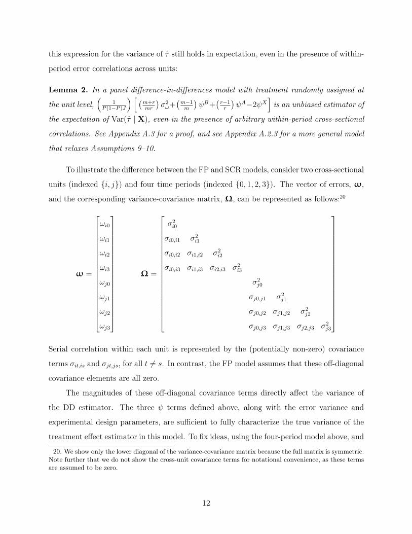
To illustrate the difference between the FP and SCRmodels, consider two cross-sectional

units (indexed i, j) and four time periods (indexed 0, 1, 2, 3). The vector of errors, ω,

and the corresponding variance-covariance matrix, Ω, can be represented as follows:20

ω =

ωi0

ωi1

ωi2

ωi3

ωj0

ωj1

ωj2

ωj3

Ω =

σ2i0

σi0,i1 σ2i1

σi0,i2 σi1,i2 σ2i2

σi0,i3 σi1,i3 σi2,i3 σ2i3

σ2j0

σj0,j1 σ2j1

σj0,j2 σj1,j2 σ2j2

σj0,j3 σj1,j3 σj2,j3 σ2j3

Serial correlation within each unit is represented by the (potentially non-zero) covariance

terms σit,is and σjt,js, for all t 6= s. In contrast, the FP model assumes that these off-diagonal

covariance elements are all zero.

The magnitudes of these off-diagonal covariance terms directly affect the variance of

the DD estimator. The three ψ terms defined above, along with the error variance and

experimental design parameters, are sufficient to fully characterize the true variance of the

treatment effect estimator in this model. To fix ideas, using the four-period model above, and

20. We show only the lower diagonal of the variance-covariance matrix because the full matrix is symmetric.Note further that we do not show the cross-unit covariance terms for notational convenience, as these termsare assumed to be zero.

12

supposing treatment is administered beginning at t = 2, these three covariance parameters

are:

ψB =σi0,i1 + σj0,j1

2

ψA =σi2,i3 + σj2,j3

2

ψX =σi0,i2 + σi1,i2 + σi0,i3 + σi1,i3 + σj0,j2 + σj1,j2 + σj0,j3 + σj1,j3

8

Alternatively, if treatment is administered beginning at t = 1, these covariance terms become:

ψB = (not defined for only 1 pre-treatment period)

ψA =σi1,i2 + σi1,i3 + σi2,i3 + σj1,j2 + σj1,j3 + σj2,j3

6

ψX =σi0,i1 + σi0,i2 + σi0,i3 + σj0,j1 + σj0,j2 + σj0,j3

6

The SCR power calculation formula above generalizes this structure to a model with J

units across m pre-treatment periods and r post-treatment periods. In this model, greater

average covariance in the pre- or post-treatment periods (ψB or ψA) increases the MDE.

Intuitively, as errors for treated and control units are more serially correlated, the benefits

of collecting multiple waves of pre- and post-treatment data are eroded. However, cross-

period covariance (ψX) enters the MDE formula negatively. This highlights a key property

of the DD estimator — because DD identifies the treatment effect off of differences between

post- and pre-treatment outcomes, greater serial correlation between pre- and post-treatment

observations makes differences caused by treatment easier to detect.

Assuming that the within-unit correlation structure does not vary systematically across

time periods, positively correlated errors will imply positive ψB, ψA, and ψX . Because ψB

and ψA enter the SCR power calculation formula positively, while ψX enters negatively, serial

correlation may either increase or decrease the MDE relative to the i.i.d. case. Specifically,

serial correlation will increase the MDE if and only if:

(m− 1

m

)ψB +

(r − 1

r

)ψA > 2ψX (6)

13

This inequality is more likely to hold in longer panels, for two reasons. First, as the number

of pre- and post-treatment periods increases,(m−1m

)and

(r−1r

)approach one. Second, the

covariance terms contributing to ψX lie farther away from the diagonal of the variance-

covariance matrix than the covariance terms contributing to ψB and ψA. Because errors

from non-adjacent time periods are likely to be less correlated than errors from adjacent

time periods, and because the number of far-off-diagonal covariances increases relatively

more quickly for ψX as the panel becomes longer, ψX is increasingly likely to be smaller

than ψB and ψA in longer panels. Together, these two effects imply that for longer panels,

the FP model is increasingly likely to yield underpowered experiments. At the same time,

using FP with short panels is likely to yield overpowered experiments.

3.3 Monte Carlo simulations

If a randomized experiment relies on a power calculation that fails to account for serial cor-

relation ex ante, its realized power may be different from the desired κ. To understand the

extent to which this matters in practice, we conduct a series of Monte Carlo simulations

comparing the FP model and the SCR model over a range of panel lengths and error cor-

relations. We simulate three cases and compute the Type I error rate and the statistical

power for each: (i) experiments that fail to account for serial correlation both ex ante and ex

post ; (ii) experiments that fail to account for serial correlation ex ante but apply the CRVE

to account for serial correlation ex post ; and (iii) experiments that both account for serial

correlation ex ante and apply the CRVE ex post.

For each set of parameter values characterizing both a data generating process and an

experimental design, we first calculate two treatment effect sizes: τFP equal to the MDE

from the FP formula, and τSCR equal to the MDE from our SCR formula. Second, we use

these parameter values to create a panel dataset from the following data generating process:

Yit = β + υi + δt + ωit (7)

14

where ωit follows an AR(1) process:

ωit = γωi(t−1) + ξit (8)

Third, we randomly assign treatment, with effect sizes τFP , τSCR, and τ 0 = 0 at the unit

level, to create three separate outcome variables. Fourth, we regress each of these outcome

variables on their respective treatment indicators and include unit fixed effects and time fixed

effects. Fifth, we compute both OLS standard errors and CRVE standard errors clustered

at the unit level, for all three regressions. We repeat steps two through five 10,000 times

for each set of parameters, calculating rejection rates of the null hypothesis τ = 0 across all

simulations. For τFP and τSCR, this rate represents the realized power of the experiment.

For the placebo τ 0, it represents the realized false rejection rate.

We test five levels of the AR(1) parameter: γ ∈ 0, 0.3, 0.5, 0.7, 0.9. For each γ,

we simulate symmetric panels with an equal number of pre-treatment and post-treatment

periods, with panel lengths ranging from 2 periods (m = r = 1) to 40 periods (m = r = 20).

We hold J , P , β, σ2υ, σ2

δ , α, and κ fixed across all simulations, and we adjust the variance

of the white noise term σ2ξ such that every simulation has a fixed idiosyncratic variance σ2

ω.

This allows γ to govern the proportion of σ2ω that is serially correlated.21 The covariance

terms ψB, ψA, and ψX have closed-form expressions under the AR(1) structure, and we use

these expressions to calculate τSCR.22 This causes τSCR to vary both with the degree of

serial correlation and panel length, whereas τFP varies only with panel length.

Figure 2 displays the results of this exercise. The left column shows rejection rates

under the FP formula using OLS standard errors, which assumes zero serial correlation both

ex ante and ex post. The middle column shows rejection rates under the FP formula using

CRVE standard errors, which accounts for serial correlation ex post only. The right column

show rejection rates under our SCR formula using CRVE standard errors, which allows for

serial correlation both ex ante and ex post. The top row plots realized power as a function

21. In an AR(1) model, the relationship between the variance of the AR(1) process and the variance of the

white noise disturbance depends on γ, with σ2ω =

σ2ξ

1−γ2 .22. We provide these formal derivations in Appendix B.1, along with further details on these Monte Carlo

simulations. We also provide additional simulation results that separately vary m and r in Appendix C.

15

of the number of pre/post-treatment periods, which should equal κ = 0.80 in a properly

designed experiment. The bottom row plots the corresponding realized false rejection rates,

which should equal the desired α = 0.05. Only the SCR formula, in conjunction with

CRVE standard errors, achieves the desired 0.80 and 0.05 across all panel lengths and AR(1)

parameters.

The left column confirms the BDM result that failing to account for serial correlation

leads to false rejection rates dramatically higher than α = 0.05. Even a modest serial

correlation parameter of γ = 0.5 yields a 20 percent probability of a Type I error, for

panels with m = r > 5. This underscores the fact that randomization cannot correct serial

correlation in panel settings, and experiments that collect multiple waves of data from the

same cross-sectional units should account for within-unit correlation over time. By contrast,

the middle and right columns apply the CRVE and reject placebo effects at the desired rate

of α = 0.05.

The middle column shows how failing to account for serial correlation ex ante can

yield dramatically overpowered or underpowered experiments. Particularly for longer panels

with m = r > 5, performing power calculations via Equation (3) may actually produce

experiments with less than 50 percent power, even though researchers intended to achieve

power of 80 percent (i.e., κ = 0.80). For a relatively high serial correlation of γ = 0.7,

simulations based on the conventional power calculation formula yield power less than 32

percent for m = r > 10. This is broadly consistent with the BDM finding that applying

the CRVE reduces statistical power, even though doing so achieves the desired Type I error

rate. By contrast, the right column applies both the SCR power calculation formula and the

CRVE, and these simulations achieve the desired power of κ = 0.80 for each value of γ.23

The middle column also highlights how failing to account for serial correlation ex ante

may either increase or decrease statistical power, as shown in Equation (6). For shorter

panels, using the FP formula instead of our SCR formula yields dramatically overpowered

experiments. While this may seem counterintuitive, (6) is increasingly unlikely to hold as m

23. As an alternative strategy for correcting false rejection rates in the presence of serial correlation, BDMsuggest collapsing data down to one pre-treatment and one post-treatment period. In Appendix A.2.4, wedemonstrate that this does not suffice for power calculations. While collapsing data enables the researcherto achieve the correct false rejection rate without knowing the true variance of their estimator, (an estimateof) this variance is required for power calculations.

16

and r decrease to 1. In the extreme case where m = r = 1, ψB and ψA do not enter, and the

only covariance term in the SCR formula is ψX , which enters negatively. These simulations

reveal that just as higher γ yields more dramatically underpowered experiments for longer

panels, higher γ yields more dramatically overpowered experiments for shorter panels.24

These results are striking. For even a modest degree of serial correlation, applying the

FP power calculation formula will not yield experiments of the desired statistical power. By

contrast, the SCR formula achieves the desired 80 percent power for all panel lengths and

AR(1) parameters. While AR(1) is a relatively simple correlation structure, it serves as a

reasonable first-approximation for more complex forms of serial correlation. Given that real-

world panel datasets exhibit enough serial correlation to produce high Type I error rates,

it stands to reason that such serial correlation can similarly impact the statistical power of

experiments if not accounted for ex ante.

4 Applications to real-world data

4.1 Bloom et al. (2015) data

In order to understand whether the differences in power demonstrated in the Monte Carlo

simulations above are meaningful in practice, we conduct an analogous simulation exercise

using a real dataset from an experiment in a developing-country setting. We use data from

Bloom et al. (2015), in which Chinese call center employees were randomly assigned to work

either from home or from the office for a nine-month period.25 The authors estimate the

24. Intuitively, serial correlation has two opposite effects on the statistical power of a DD estimator. Itdecreases power by reducing the effective number of observations for each cross-sectional unit, and it increasespower by increasing the signal in estimating treatment effects off of a post−pre difference. In shorter panels,this second effect tends to dominate. See Appendix C for additional short-panel results.25. This dataset consists of weekly performance measures for the 249 workers enrolled in the experiment

between January 2010 and August 2011. We keep only those individuals who have non-missing performancedata for the entire pre-treatment period, leaving us with a balanced panel of 79 individuals over 48 pre-treatment weeks (a different sample from that in the paper). Our purpose with this exercise is not tocomment on the statistical power of the original paper, but rather to investigate the importance of accountingfor serial correlation ex ante in real experimental data. Appendix B.2 provides more information on thissimulation dataset, including summary statistics.

17

following equation to derive the central result, reported in Table 2 in the original paper:

Performanceit = αTreati × Experimentt + βt + γi + εit (9)

This is a standard DD estimating equation with fixed effects for individual i and week t.

From this model’s residuals, we estimate an AR(1) parameter of γ = 0.233, which is highly

statistically significant and indicates that these worker performance data exhibit weak serial

correlation.

We perform Monte Carlo simulations on this dataset that are analogous to those pre-

sented above. We subset consecutive periods of the Bloom et al. (2015) dataset to create

panels ranging in length from 2 periods (m = r = 1) to 40 periods (m = r = 20). For each

simulation panel length, we randomly assign three treatment effect sizes, τFP , τAR(1), and

τSCR, at the individual level and estimate Equation (9) separately for each treatment effect

size. We calibrate τFP using the FP formula that assumes no serial correlation; τAR(1) using

the SCR formula with ψ parameters consistent with an AR(1) error structure of γ = 0.233;

and τSCR using the SCR formula with non-parametrically estimated ψω parameters. We

define σ2ω, ψBω , ψAω and ψXω to be the estimated analogues of σ2

ω, ψB, ψA, and ψX , where the

subscript ω denotes the variance/covariance of residuals rather than errors.26

Figure 3 reports the results of this exercise, demonstrating that only the SCR formula

achieves the desired statistical power in the Bloom et al. (2015) data. Failing to account for

serial correlation leads to experiments that deviate dramatically from 80 percent power, even

in the presence of relatively weak serial correlation. For an experiment with 12 pre/post-

treatment periods, applying the FP formula with κ = 0.80 yields an experiment with only 35

percent power. This is consistent with our results from simulated data, demonstrating that

researchers can calibrate a panel RCT to 80 percent power if the ex ante formula properly

accounts for the within-unit correlation structure of the data.

26. Appendix D.1 outlines how to estimate these parameters. For all three treatment effects, we estimatethe value of σ2

ω estimated from residuals.

18

4.2 Pecan Street data

Having demonstrated the importance of properly accounting for serial correlation using data

from an RCT in a developing country setting, we now turn to a much higher-frequency

dataset with higher serial correlation: household electricity consumption in the United States

(Pecan Street (2016)).27 Electricity consumption data tend to exhibit high within-household

autocorrelation, making them particularly well-suited for this study. Additionally, RCTs

using energy consumption data are becoming increasingly common in economics, making

our Pecan Street application relevant to this growing literature.28

We aggregate these data to four different temporal levels: hourly, daily, weekly, and

monthly, each with a different correlation structures and amounts of idiosyncratic variation,

which sheds light on the performance of different power calculation approaches over a range

of underlying error structures. We conduct Monte Carlo simulations on all four versions of

the Pecan Street data to assess the performance of alternative power calculation assumptions.

These follow the same procedure as the Bloom et al. (2015) simulations.29 Figure 4 shows

that in all four versions of the Pecan Street data, realized power sharply deviates from the

desired 80 percent under both the FP assumption of i.i.d. errors and an assumed AR(1)

structure. We achieve correctly powered experimental designs only by applying the SCR

method, which accounts for the full covariance structure of the Pecan Street data. This

results holds at both high and low temporal frequencies, and is consistent with the Bloom

et al. (2015) simulations.

4.3 Power calculations in real data

We can use the SCR formula to perform power calculations, which quantify the tradeoff be-

tweenMDE and J over different panel lengths. In order to operationalize the SCR formula,

27. Pecan Street is a research organization, based at the University of Texas at Austin, that makes high-resolution energy usage data available to academic researchers. The raw data, which are available with a loginfrom https://dataport.pecanstreet.org/data/interactive, consist of hourly electricity consumptionfor 699 households over 26,888 hours. Appendix B.3 describes the data, including summary statistics, infurther detail.28. For example, see Allcott (2011), Jessoe and Rapson (2014), Ito, Ida, and Tanaka (forthcoming), Fowlie,

Greenstone, and Wolfram (forthcoming), Fowlie et al. (2017), and Allcott and Greenstone (2017). There isalso a large quasi-experimental literature that uses energy consumption data.29. Appendix B.3 provides further details on these simulations.

19

researchers must assume values for σ2ω, ψB, ψA, and ψX that reflect the error structure likely

to be present in their (future) experimental datasets. In the best case scenario, researchers

will have access to data that are representative of what will be collected in the field, and they

can simply calculate these variance and covariance terms from this pre-existing dataset.30

Plugging these estimates into the SCR formula, researchers can evaluate the tradeoffs be-

tween different experimental design elements, such as the desired power of the experiment,

the number of units to recruit, the number of observations to collect for each unit, and the

expected effect size of the intervention.

We perform this procedure on the daily Pecan Street dataset to imitate the design

of an experiment that affects household electricity consumption. We do so both under the

assumption of uncorrelated errors and also allowing for arbitrary correlations among the error

terms of a household using the FP formula and the SCR formula, respectively. For simplicity,

we consider only balanced panels of households with the same number of observations before

and after the experimental intervention (i.e.m = r). For each experiment length, we estimate

the average σ2ω and ψω terms from the daily Pecan Street dataset, and we assume constant

values for the remaining parameters.31

We plot the results of this exercise in Figure 5. The left panel depicts power calculations

using the FP formula, which assumes an i.i.d. error structure. The right panel applies the

SCR formula to compute the number of units required for the same set of MDEs, using our

non-parametric estimates of ψBω , ψAω , and ψXω to reflect the real error structure of the data.

Each curve corresponds to an experiment of a particular length, ranging from m = r = 1

to m = r = 12; the curves plot the number of households required to achieve 80 percent

power as a function of the MDE. For each MDE, fewer households are required as the

length of the experiment increases. However, the “naive” power calculation always implies a

substantially smaller number of households than the SCR power calculation - for example,

30. Appendix D.1 provides details on how to estimate σ2ω, ψ

Bω , ψ

Aω , and ψXω from pre-existing data, and

Appendix E proves that power calculations using estimated parameters recover the sameMDE in expectationas those using true parameters. The plausibility of estimating these parameters will vary across settings.Researchers with implementing partners that have access to large amounts of historical data may use thesedata to estimate σ2

ω, ψBω , ψ

Aω , and ψXω . On the other hand, this may not be possible for experiments

in completely unstudied settings. See Appendix D.3 for more details on how to overcome a lack of pre-experimental data.31. See Appendix B.4 for details.

20

with m = r = 12, the “naive” power calculation suggests the researcher only needs 106

households to achieve an MDE of 5 percent; the SCR power calculation implies that the

required sample size is 354 households - over 3 times greater. Hence, if a researcher in this

setting applies the CRVE ex post but assumes i.i.d. errors ex ante, he will likely include too

few households to achieve the desired statistical power.

5 Power calculations in practice

5.1 Trading off units and time periods

Recruiting participants, administering treatment, and collecting data are all costly, and

these implementation costs are often the limiting factor in study size. We can use the power

calculation framework to conceptualize the optimal design of a panel RCT given a budget,

by couching it in a simple constrained optimization problem of the following form:

minP,J,m,r

MDE(P, J,m, r) s.t. C(P, J,m, r) ≤ B (10)

where C(P, J,m, r) is the cost of conducting an experiment and B is the experiment’s budget.

The budget constraint creates a fundamental tradeoff between including additional units

and including additional time periods in the experiment, since each comes at a cost.32 This

tradeoff also arises from differences in the marginal effects of units and time periods on the

MDE. Using the SCR power calculation formula, the “elasticities” of theMDE with respect

to number of units and number of time periods are:

32. Researchers may also adjust P to make an experimental design more cost effective. An RCT willhave the lowest MDE at P = 0.5, but if control units are cheap compared to treatment units, the samepower may be achieved at lower cost by decreasing P and increasing J . See Duflo, Glennerster, and Kremer(2007) for more details. We also typically consider α and κ to be fixed “by convention.” While α is theproduct of research norms, and therefore relatively inflexible, researchers may want to adjust κ. 1 − κ isthe probability of being unable to distinguish a true effect from 0. In lab experiments which are cheaplyreplicated, researchers may accept κ < 0.80, whereas in large, expensive field experiments that can only beconducted once, researchers may instead wish to set κ > 0.80. Researchers may also choose to size theirexperiments such that they achieve a power of 80 percent for the smallest economically meaningful effect,even if they expect the true MDE to be larger.

21

∂MDE/MDE

∂J/J= −1

2

∂MDE/MDE

∂m/m= −1

2

[σ2ω

m− ψB

m− (m− 1)∂ψ

B

∂m+ 2m∂ψX

∂m(m+rmr

)σ2ω +

(m−1m

)ψB +

(r−1r

)ψA − 2ψX

]∂MDE/MDE

∂r/r= −1

2

[σ2ω

r− ψA

r− (r − 1)∂ψ

A

∂r+ 2r ∂ψ

X

∂r(m+rmr

)σ2ω +

(m−1m

)ψB +

(r−1r

)ψA − 2ψX

]

There is a constant elasticity of MDE with respect to J of −0.5, meaning that a 1

percent increase in the number of units always yields a 0.5 percent reduction in the MDE.

However, the elasticity of MDE with respect to m and r varies as a function of the error

structure and the number of time periods.33 For some parameter values, this elasticity can

be positive, such that increasing the length of the experiment would actually increase the

MDE. This may seem counter-intuitive, but adding time periods can reduce the average

covariance between pre- and post-treatment observations, ψX , which introduces more noise

in the estimation of pre- vs. post-treatment difference. For relatively short panels with errors

that exhibit strong serial correlation, this effect can dominate the benefits of collecting more

time periods.

Figure 6 illustrates the fact that additional time periods may either increase or decrease

statistical power. The left panel plots theMDE of an experiment as a function of the number

of pre- and post-treatment waves, holding the number of units J constant. The right panel

depicts the tradeoff between additional units and additional time periods by plotting the

combinations of J and m = r that yield a given MDE. To analytically construct these

curves, we use the SCR formula and assume that the error structure is AR(1) with varying

γ values.

At low to moderate levels of serial correlation, increasing the panel length always reduces

the MDE for a given J and, likewise, reduces the J required to achieve a given MDE.

However, at higher levels of serial correlation, this relationship is no longer monotonic. For

33. Note that J , m, and r must all be integer-valued, hence these derivatives serve as continuous approxi-mations of discrete changes in these parameters. Likewise, the partial derivatives of ψB , ψA, and ψX withrespect to m and r are not technically defined, as these covariance terms are averaged over discrete numbersof periods (as shown in Assumption 10).

22

γ ≥ 0.6, marginally increasing m or r in a relatively short panel increases the MDE for

a given J and, likewise, increases the J required to achieve a given MDE. This suggests

that for experiments using highly correlated data, such as any of the four Pecan Street

datasets above, additional periods of data might decrease statistical power if the panel is not

sufficiently long.34

5.2 ANCOVA

Many published and pre-registered ongoing experiments in economics estimate treatment

effects using analysis of covariance (ANCOVA) methods.35 To do this, the econometrician

estimates the following specification using post-treatment data only:

Yit = α + τDi + θY Bi + εit (11)

where Y Bi =

∑0t=−m+1 Yit is the pre-treatment average value of the dependent variable for

unit i. This estimator has become popular in economics, as it is more efficient than the DD

model with the same number of periods (McKenzie (2012)).

Frison and Pocock (1992) also derive what has become the standard formula for AN-

COVA power calculations (henceforth FP ANCOVA), which we adapt to our notation:

MDE ≈ (tJ1−k + tJα/2)

√(1

P (1− P )J

)[(1− θ)2σ2

υ +

(θ2

m+

1

r

)σ2ω

](12)

34. McKenzie (2012) argues that stronger unit-specific shocks (i.e. higher σ2υ) can erode the benefits

of collecting additional waves of data; this result extends that argument to within-unit serial correlation,demonstrating that higher autocorrelation in the idiosyncratic error term can similarly erode – and evenreverse – the benefits of increased panel length.35. In a randomized setting, where unit fixed effects are not needed for identification, this method may

be preferred to DD because it more efficiently estimates τ (Frison and Pocock (1992)). McKenzie (2012)comment thats, with i.i.d. error structures, ANCOVA is always more efficient than the DD model with thesame number of periods, but that these gains are eroded as the intracluster correlation coefficient increases.Neither paper handles the fully general case of arbitrary serial correlation. Teerenstra et al. (2012) beginswith a similar setup for the ANCOVA framework, but considers the m = r = 1 case only, obviating the needto address the CRVE-related issues raised here.

23

where θ = mσ2υ

mσ2υ+σ

2ω.36 Importantly, deriving this formula under serial correlation necessitates

an additional simplifying assumption for analytical tractability: we must assume away time

shocks.37 Under this strong assumption, we also derive the variance of the ANCOVA allowing

for serial correlation, along with the corresponding serial-correlation-robust power calculation

formula (henceforth SCR ANCOVA):

Var(τ | X) ≈ 1P (1−P )J

[(1− θ)2σ2

υ +(θ2

m+ 1

r

)σ2ω + θ2(m−1)

mψB + r−1

rψA − 2θψX

](13)

MDE ≈ (tJ1−κ + tJα/2)×√1

P (1−P )J

[(1− θ)2σ2

υ +(θ2

m+ 1

r

)σ2ω + θ2(m−1)

mψB + r−1

rψA − 2θψX

](14)

where θ = mσ2υ+mψ

X

mσ2υ+σ

2ω+(m−1)ψB .

38

As in Section 3, we compare the FP ANCOVA formula to the SCR ANCOVA formula

by simulating data with an AR(1) error term and varying panel lengths. For each level

of the AR(1) parameter and panel length, we compute the treatment effect size τ implied

from the FP ANCOVA or SCR ANCOVA formulas. Next, we simulate 10,000 experiments,

randomly assigning units to treatment with the appropriate effect size.39 For each simulated

36. The FP ANCOVA formula presented here differs slightly from that in Frison and Pocock (1992) andMcKenzie (2012) because previous derivations have assumed that the true data generating process followsEquation (12), where outcomes are determined in part by pre-treatment values of the outcome. We insteadassume that that there are unit-specific random effects, as in Assumption 6. The FP ANCOVA modelassumes that time shocks are deterministic and have no variance, or σ2

δ = 0; we instead must assume thatthere are no time shocks for analytical tractability. While both data generating processes yield identicaltreatment effect estimators, they imply different variances of this estimator. As in Frison and Pocock (1992),this formula is approximate because we ignore sampling error in the estimation of θ, which approaches zeroas the number of units increases.37. A critical step in the derivation of the ANCOVA model with time shocks and arbitrary serial correlation

requires us to calculate a conditional expectation that depends on the error term εit and the pre-period meanY Bi of every unit in the experiment, which becomes analytically intractable for any reasonable number ofexperimental units. See Appendix A.2.5 for more details. By contrast, the variance of the DD estimatordepends on the distribution of errors conditional on only the treatment indicator, which is orthogonal to theerror terms by randomization.38. We present the formal derivation of the SCR ANCOVA formula in Appendix A.2.5. For analytical

tractability, we assume that the ψ parameters are uniform across all units. We also ignore sampling error inthe estimation of θ, which approaches zero as the number of units increases (Frison and Pocock (1992) andMcKenzie (2012) also make this simplification). Through additional Monte Carlo simulations, we confirmthat neither of these assumptions is likely to affect statistical power.39. In keeping with the assumptions of these models, we do not include time shocks in the data generating

process.

24

experiment, we estimate τ using the ANCOVA estimator, and record whether τ is statistically

different from zero with clustered standard errors. We calculate realized power as the fraction

of experiments that reject the null hypothesis of τ = 0. Figure 7 presents the results of this

exercise. While the FP ANCOVA formula produces properly-powered experiments only when

errors are i.i.d., the SCR ANCOVA is robust to all levels of AR(1) serial correlation.

Even though the SCR ANCOVA formula outperforms the FP ANCOVA formula in

the presence of serial correlation, we do not recommend that researchers use this formula

in real-world applications. Time shocks with non-zero variance are a common feature of

panel data, and assuming them away may result in improperly powered experiments.40 For

this reason, we suggest that researchers either conduct power calculations by simulation (as

discussed below) or perform power calculations using the SCR DD formula, which yields

correctly powered DD experiments using real-world data. Power calculations based on ex

ante assumptions of the DD estimator will understate the realized power from estimating a

more-efficient ANCOVA model ex post.41

5.3 A simulation-based approach

In this paper, we develop an analytical framework for performing power calculations in a

DD model with panel data that have a non-i.i.d. error structure. Shifting from the i.i.d.

model to a non-i.i.d. model increases the number of parameters required to calibrate a

DD power calculation formula. This reveals a fundamental challenge of analytical power

calculations: more complex experimental designs and data generating processes require more

complex treatment effect estimators, which in turn have analytic variance expressions that

are increasingly difficult to derive and parameterize. For example, if we relax the assumption

of randomization and instead consider a quasi-experimental DD design, where cross-sectional

correlations remain important, the expression for Var(τ) includes 13 separate ψ parameters

40. See Appendix C where we apply the SCR ANCOVA formula to the Bloom et al. (2015) data. We donot achieve the desired power in simulated experiments due to the unaccounted-for time shocks that existin this real-world dataset.41. This will always be true with i.i.d. errors and with serial correlation in the absence of time shocks; the

full result for the ANCOVA model including time shocks has yet to be proven.

25

— each of which would need to be non-parametrically estimated to fully characterize the

error structure of the data and conduct an analytical power calculation.42

In light of these challenges, we recommend performing power calculations via simu-

lation rather than by using analytic formulas, in cases where researchers have access to a

pre-existing dataset that is representative of their future experimental data. Simulation-

based power calculations follow a straightforward Monte Carlo process, where each simula-

tion implements the proposed estimating equation over a range of assumed treatment effect

sizes (τ), numbers of units (J), proportion of units treated (P ), and panel lengths (m and

r).43 Calculating the average rejection rates of the null hypothesis τ = 0 over all simula-

tions will reveal the statistical power of each parameterization, and researchers can compare

power across parameterizations to find their preferred values of P , J , m, and r. Impor-

tantly, simulation-based power calculations do not require researchers to estimate Var(τ) as

a function of the underlying error structure in the data. This allows for greater flexibility

in selecting research designs, and easily facilitates comparisons across alternative estimating

equations.44

Simulation-based power calculations allow researchers to leverage any representative

pre-existing data that may exist, and our analytical results provide key intuition for in-

terpreting this simulation output. Given that power calculations via simulation are com-

putationally intensive and necessitate a grid search over the full space of candidate design

parameters, researchers may begin by using analytical power calculation formulas to narrow

the range of plausible parameter values. In the absence of representative data ex ante, re-

searchers may apply analytical techniques (with appropriate sensitivity analyses) to inform

experimental design. It may still be possible to calibrate the variance-covariance parame-

ters in the serial-correlation-robust power calculation formula, even if the ideal pre-existing

dataset is not available.

42. See Appendix A.2.3 for the full derivation and resulting power calculation equation.43. For each simulation, the researcher re-randomizes PJ units into treatment, adds τ to treated units’

outcomes for all post-treatment periods, and estimates τ using her preferred variance estimator. We providefurther guidance on simulation-based power calculations in Appendix D.2.44. For example, a simulation-based power calculation for a proposed experiment using hourly electricity

consumption data could compare the standard DD specification with individual and time fixed effects to analternative specification that also includes group-specific time trends, without needing to formally derive anexpression for Var(τ) under this alternative model.

26

6 Conclusion

Randomized experiments are costly, and it is important that researchers avoid underpowered

experiments that are not informative, as well as dramatically overpowered experiments that

waste resources. Statistical power calculations help researchers to calibrate the sample size

of experiments ex ante, such that they are likely to collect enough data to detect treatment

effects of a meaningful size, while also unlikely to collect excessive amounts of costly data.

As data collection becomes easier and cheaper, panel data are becoming increasingly com-

mon in randomized experiments. Temporally disaggregated data allow researchers to ask

new questions, and to apply a wider range of empirical methods to answer these questions

(McKenzie (2012)).

In this paper, we identify a fundamental mismatch between existing ex ante power

calculation techniques and ex post inference in panel data settings. We develop new tools

to incorporate serial correlation into the design of panel RCTs. We derive the variance of a

panel difference-in-differences estimator allowing for arbitrary within-unit correlation, which

we use to update the conventional differences-in-differences power calculation formula derived

by Frison and Pocock (1992). This new “serial-correlation-robust” formula is consistent with

the CRVE variance estimator, which has become standard practice in ex post analysis of panel

RCTs. We use Monte Carlo analyses to demonstrate that our updated power calculation

formula achieves the desired statistical power, whereas the conventional formula is likely to

produce either dramatically underpowered or overpowered experiments in the presence of

serially correlated errors. These results hold in real data from a panel RCT in China, and

for household electricity consumption data similar to that used in panel RCTs in the energy

economics literature.

Our work highlights the need to carefully consider the assumptions that will enter ex

post analysis when calibrating the design of experiments ex ante. The serial-correlation-

robust power calculation framework allows researchers to conduct power calculations that

correctly account for within-unit correlation, and provides intuition about these calcula-

tions under non-i.i.d. errors. We extend the main results by providing researchers with a

framework for trading off units for effect sizes that takes cost into account; discussing the

27

ANCOVA estimator in the presence of serial correlation; and discussing implementation of

power calculations in practice.45 Ultimately, this paper serves as a useful starting point

for power calculations with serial correlation. Future research should seek to extend this

framework to accommodate heterogeneous effects, cluster-randomized trials, and ANCOVA

models with time shocks.

ReferencesAbadie, Alberto, Susan Athey, Guido W. Imbens, and Jeffrey Wooldridge. 2017. “When

Should You Adjust Standard Errors for Clustering?” ArXivWorking Paper No. 1710.02926.

Allcott, Hunt. 2011. “Social Norms and Energy Conservation.” Journal of Public Economics95 (9): 1082–1095.

Allcott, Hunt, and Michael Greenstone. 2017. “Measuring the Welfare Effects of ResidentialEnergy Efficiency Programs.” National Bureau of Economic Research Working PaperNo. 23386.

Angrist, Joshua D., and Jorn-Steffen Pischke. 2010. “The Credibility Revolution in Empir-ical Economics: How Better Research Design is Taking the Con out of Econometrics.”Journal of Economic Perspectives 24 (2): 3–30.

Arellano, Manuel. 1987. “Computing Robust Standard Errors for Within-Group Estimators.”Oxford Bulletin of Economics and Statistics 49 (4): 431–34.

Athey, Susan, and Guido Imbens. 2017. “The State of Applied Econometrics: Causality andPolicy Evaluation.” Journal of Economic Perspectives 31 (2): 3–32.

Athey, Susan, and Guido W. Imbens. 2016. “The Econometrics of Randomized Experiments.”Working Paper.

Atkin, Azam, David aand Chaudhry, Shamyla Chaudry, Amit K. Khandelwal, and EricVerhoogen. 2017. “Organization Barriers to Technology Adoption: Evidence from Soccer-Ball Producers in Pakistan.” The Quarterly Journal of Economics 132 (3): 1101–1164.

Atkin, David, Amit K. Khandelwal, and Adam Osman. 2017. “Exporting and Firm Perfor-mance: Evidence from a Randomized Experiment.” The Quarterly Journal of Economics132 (2): 551–615.

Baird, Sarah, J. Aislinn Bohren, Craig McIntosh, and Berk ’Ozler. forthcoming. “OptimalDesign of Experiments in the Presence of Interference.” Review of Economics and Statis-tics.

45. We have an accompanying software package, pcpanel, which makes our power calculation methodeasily accessible and user-friendly. The Stata package pcpanel is currently is available from ssc, with an Rversion to follow shortly, which will be available from CRAN.

28

Bertrand, Marianne, Esther Duflo, and Sendhil Mullainathan. 2004. “How Much Should WeTrust Differences-In-Differences Estimates?” The Quarterly Journal of Economics 119(1): 249–275.

Blattman, Christopher, Nathan Fiala, and Sebastian Martinez. 2014. “Generating SkilledSelf-Employment in Developing Countries: Experimental Evidence from Uganda.” TheQuarterly Journal of Economics 129 (2): 697–752.

Bloom, Howard S. 1995. “Minimum Detectable Effects: A Simple Way to Report the Statis-tical Power of Experimental Designs.” Evaluation Review 19 (5): 547–556.

Bloom, Nicholas, Benn Eifert, Aprajit Mahajan, David McKenzie, and John Roberts. 2013.“Does Management Matter? Evidence from India.” The Quarterly Journal of Economics128 (1): 1–51.

Bloom, Nicholas, James Liang, John Roberts, and Zhichun Jenny Ying. 2015. “Does Workingfrom Home Work? Evidence from a Chinese Experiment.” The Quarterly Journal ofEconomics 130 (1): 165–218.

Cameron, A. Colin, Jonah B. Gelbach, and Douglas L. Miller. 2008. “Bootstrap-Based Im-provements for Inference with Clustered Errors.” Review of Economics and Statistics 90(3): 414–427.

Cameron, A. Colin, and Douglas L. Miller. 2015. “A Practitioner’s Guide to Cluster-RobustInference.” Journal of Human Resources 50 (2): 317–372.

Campbell, Cathy. 1977. “Properties of Ordinary and Weighted Least Square Estimatorsof Regression Coefficients for Two-Stage Samples.” Proceedings of the Social StatisticsSection, American Statistical Association: 800–805.

Card, David, Stefano DellaVigna, and Ulrike Malmendier. 2011. “The Role of Theory inField Experiments.” Journal of Economic Perspectives 25 (3): 39–62.

Cohen, Jacob. 1977. Statistical Power Analysis for the Behavioral Sciences. New York, NY:Academic Press.

Duflo, Esther, Rachel Glennerster, and Michael Kremer. 2007. “Using Randomization inDevelopment Economics Research: A Toolkit.” Chap. 61 in Handbook of DevelopmentEconomics, edited by Paul T. Schultz and John A. Strauss, 3895–3962. Volume 4. Ox-ford, UK: Elsevier.

Fowlie, Meredith, Michael Greenstone, and Catherine Wolfram. Forthcoming. “Do EnergyEfficiency Investments Deliver? Evidence from the Weatherization Assistance Program.”

Fowlie, Meredith, Catherine Wolfram, C. Anna Spurlock, Annika Todd, Patrick Baylis, andPeter Cappers. 2017. “Default Effects and Follow-on Behavior: Evidence from an Elec-tricity Pricing Program.” National Bureau of Economic Research Working Paper No.23553.

29

Frison, L., and S. J. Pocock. 1992. “Repeated Measures in Clinical Trials: Analysis UsingMean Summary Statistics and its Implications for Design.” Statistics in Medicine 11(13): 1685–1704.

Glennerster, Rachel, and Kudzai Takavarashi. 2013. Running Randomized Evaluations: APractical Guide. Princeton, NJ: Princeton University Press.

Ito, Koichiro, Takanori Ida, and Makoto Tanaka. Forthcoming. “Moral Suasion and EconomicIncentives: Field Experimental Evidence from Energy Demand.” American EconomicJournal: Economic Policy.

Jessoe, Katrina, and David Rapson. 2014. “Knowledge Is (Less) Power: Experimental Evi-dence from Residential Energy Use.” American Economic Review 104 (4): 1417–1438.

McKenzie, David. 2012. “Beyond Baseline and Follow-up: The Case for More T in Experi-ments.” Journal of Development Economics 99 (2): 210–221.

. 2017. “Identifying and Spurring High-Growth Entrepreneurship: Experimental Evi-dence from a Business Plan Competition.” American Economic Review 107 (8): 2278–2307.

Moulton, Brent. 1986. “Random group effects and the precision of regression estimates.”Journal of Econometrics 32 (3): 385–397.

Murphy, Kevin, Brett Myors, and Allen Wolach. 2014. Statistical Power Analysis: A Simpleand General Model for Traditional and Modern Hypothesis Tests. 4th ed. New York,NY: Routledge.

Pecan Street. 2016. “Dataport.” https://dataport.pecanstreet.org/.

Rubin, Donald B. 1974. “Estimating Causal Effects of Treatments in Randomized and Non-randomized Studies.” Journal of Educational Psychology 66 (5): 688–701.

Teerenstra, Steven, Sandra Eldridge, Maud Graff, Esther de Hoop, and George F. Borm.2012. “A simple sample size formula for analysis of covariance in cluster randomizedtrials.” Statistics in Medicine 31 (20): 2169–2178.

White, Halbert. 1984. Asymptotic Theory for Econometricians. 1st ed. San Diego, CA: Aca-demic Press.

30

Tables and Figures

Figure 1: Hypothesis testing framework

τ = MDEτ = 0

α/2

κ

Notes: This figure displays the theoretical underpinnings of statistical power calculations. The black curverepresents the distribution of the treatment effect estimator τ under the null hypothesis of a zero effect. Fora chosen significance level α, we will reject this null if τ lies above (below) the 1 − α/2 (α/2) percentile ofthe distribution. The gray-shaded area represents the likelihood of a Type I error. The blue curve is thedistribution of τ under the hypothesis that τ is equal to some other value, where this value is the minimumdetectable effect (MDE) that yields a statistical power of κ. Given that τ = MDE and given the samplesize J , the shaded blue area is the power of this test. The unshaded area to the left of the critical value (thedashed gray line) and under the blue distribution represents the likelihood of committing a Type II error.

31

Figure 2: Traditional methods result in improperly powered experiments in AR(1) data

.2

.4

.6

.8

1

Po

we

r

0 5 10 15 20

Pre/post periods

OLS SE

Frison and Pocock

.2

.4

.6

.8

1

Po

we

r

0 5 10 15 20

Pre/post periods

Clustered SE

Frison and Pocock

.2

.4

.6

.8

1

Po

we

r

0 5 10 15 20

Pre/post periods

Clustered SE

Serial−Correlation−Robust

0

.2

.4

.6

Fa

lse

re

jectio

n r

ate

0 5 10 15 20

Pre/post periods

0

.2

.4

.6

Fa

lse

re

jectio

n r

ate

0 5 10 15 20

Pre/post periods

0

.2

.4

.6

Fa

lse

re

jectio

n r

ate

0 5 10 15 20

Pre/post periods

0 0.3 0.5 0.7 0.9

AR(1) γ

Notes: This figure displays power and rejection rates from performing power calculations with three differentsets of assumptions on data generated with AR(1) processes with differing levels of serial correlation anddiffering panel lengths (ranging from 2, m = r = 1, to 40, m = r = 20). In the left column, we apply theformula of Frison and Pocock (1992) (Equation (3)), and use OLS standard errors ex post, in line with theassumptions of this formula. In the middle column, we again apply calibrate power calculations using Frisonand Pocock (1992)’s formula, but cluster standard errors ex post — which is inconsistent with the ex anteformula, but corrects for within-unit serial correlation following Bertrand, Duflo, and Mullainathan (2004).In the right column, we apply the serial-correlation-robust power calculation formula to account for non-i.i.d.errors ex ante, and we cluster standard errors at the individual level ex post. As expected, this third set ofsimulations achieves the desired 80 percent power and 5 percent false rejection rate.

32

Figure 3: Power simulations for Bloom et al. (2015) data

.2

.4

.6

.8

1

Po

we

r

0 5 10

Pre/post periods

Frison and Pocock AR(1) imposed Serial−Correlation−Robust

Notes: This figure shows results from Monte Carlo simulations using Bloom et al. (2015)data. Each curve displays the relationship between realized power and the number ofpre/post periods used, applying different ex ante assumptions. The long-dashed line usesthe Frison and Pocock (1992) formula. The short-dashed line uses the serial-correlation-robust formula, under the assumption that the error structure is AR(1). We estimate theAR(1) parameter via Equation (8). The solid line applies the serial-correlation-robustformula, where we non-parametrically generate estimates of ψBω , ψ

Aω , and ψ

Xω terms using

the Bloom et al. (2015) dataset. All three sets of simulations apply the CRVE ex post,clustering at the individual level. Only the serial-correlation-robust power calculationformula achieves the desired power of 80 percent, even though the Bloom et al. (2015)data exhibit relatively weak serial correlation.

33

Figure 4: Power simulations for Pecan Street data

.2

.4

.6

.8

1

Pow

er

0 4 8 12

Pre/post periods

Hourly

.2

.4

.6

.8

1

Pow

er

0 4 8 12

Pre/post periods

Daily

.2

.4

.6

.8

1

Pow

er

0 4 8 12

Pre/post periods

Weekly

.2

.4

.6

.8

1

Pow

er

0 4 8 12

Pre/post periods

Monthly

Frison and Pocock AR(1) imposed Serial−Correlation−Robust

Notes: This figure shows results from Monte Carlo simulations using the Pecan Street electricity data,collapsed to different levels of aggregation. Each curve displays the relationship between power and thenumber of pre/post periods used, applying different ex ante assumptions. The long-dashed lines use theFrison and Pocock (1992) formula (Equation (3)). The short-dashed lines use Equation (5) assuming anAR(1) error structure, where we estimate the AR(1) parameters by estimating Equation (8) separately foreach dataset. The solid lines apply Equation (5), by estimating separate covariance components of ψBω , ψ

Aω ,

and ψXω terms using residuals from each Pecan Street dataset. All simulations apply the CRVE ex post,clustering at the household level. For each temporal resolution, only the serial-correlation-robust powercalculation formula achieves desired power of 80 percent.

34

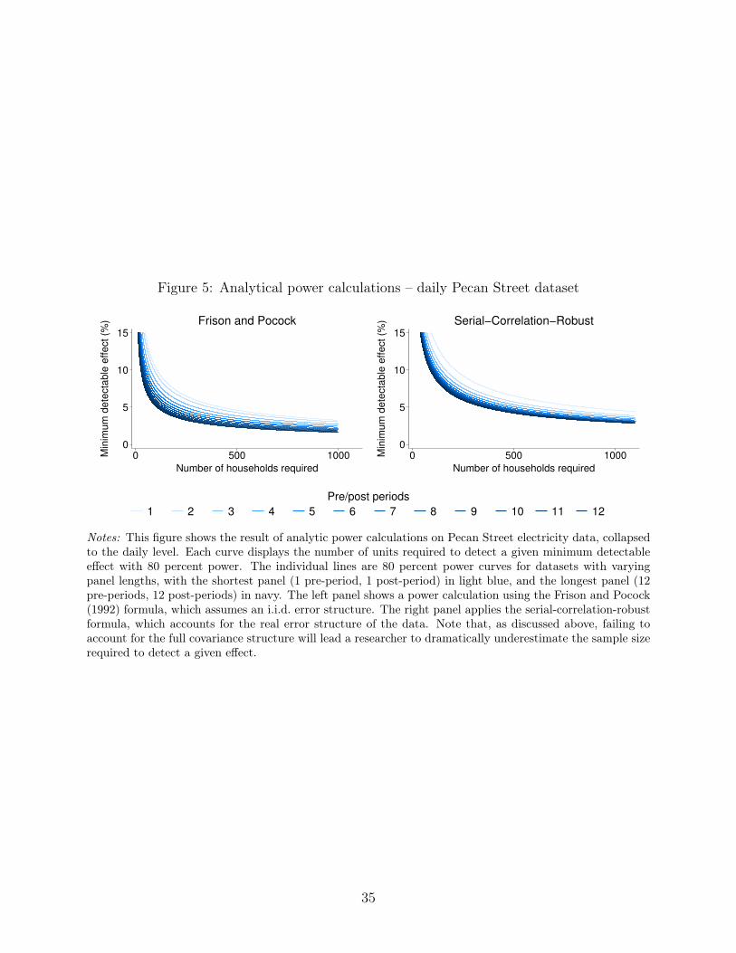
Figure 5: Analytical power calculations – daily Pecan Street dataset

0

5

10

15

Min

imum

dete

cta

ble

effect (%

)

0 500 1000

Number of households required

Frison and Pocock

0

5

10

15

Min

imum

dete

cta

ble

effect (%

)

0 500 1000

Number of households required

Serial−Correlation−Robust

1 2 3 4 5 6 7 8 9 10 11 12

Pre/post periods

Notes: This figure shows the result of analytic power calculations on Pecan Street electricity data, collapsedto the daily level. Each curve displays the number of units required to detect a given minimum detectableeffect with 80 percent power. The individual lines are 80 percent power curves for datasets with varyingpanel lengths, with the shortest panel (1 pre-period, 1 post-period) in light blue, and the longest panel (12pre-periods, 12 post-periods) in navy. The left panel shows a power calculation using the Frison and Pocock(1992) formula, which assumes an i.i.d. error structure. The right panel applies the serial-correlation-robustformula, which accounts for the real error structure of the data. Note that, as discussed above, failing toaccount for the full covariance structure will lead a researcher to dramatically underestimate the sample sizerequired to detect a given effect.

35

Figure 6: Analytical power calculations with increasing panel length

0

.2

.4

.6

.8

Min

imu

m d

ete

cta

ble

eff

ect

(SD

of

ω)

0 20 40 60 80 100

Pre/post periods

0

50

100

150

Nu

mb

er

of

un

its r

eq

uire

d

0 20 40 60 80 100

Pre/post periods

0 0.3 0.5 0.7 0.9

AR(1) γ

Notes: This figure displays the results of analytical power calculations using the serial-correlation-robustformula for varying AR(1) parameters. The left panel shows the tradeoff between the minimum detectableeffect (MDE) and the number of time periods (m = r) for varying levels of serial correlation, holding thenumber of units fixed at J = 100 and normalizing MDE by the standard deviation of ωit. At low levelsof γ, the MDE declines monotonically in m and r. However, for higher γ, increasing m and r actuallyincreases the MDE when m = r is relatively small and decreases the MDE when m = r is relatively large.The right panel shows the relationship between the number of units (J) and number of pre/post periods(m = r) required to detect an MDE equal to one standard deviation of ωit. Similarly, for low levels ofserial correlation, the trade-off between J and m = r is monotonic. However, as γ increases, adding periodsin short panels necessitates a greater number of units to achieve the same MDE, while adding periods inlonger panels means that fewer units are required to achieve the same MDE.

36

Figure 7: Traditional ANCOVA methods fail under serial correlation

.2

.4

.6

.8

1

Po

we

r

0 5 10 15 20

Pre/post periods

Clustered SE

Frison and Pocock

.2

.4

.6

.8

1

Po

we

r

0 5 10 15 20

Pre/post periods

Clustered SE

Serial−Correlation−Robust

Notes: This figure displays power from performing power calculations for the ANCOVA estimator under twosets of assumptions on data generated with AR(1) processes with differing levels of serial correlation anddiffering panel lengths (ranging from 2, m = r = 1, to 40, m = r = 20). In the left panel, we apply the Frisonand Pocock (1992) ANCOVA power calculation formula. In the right panel, we use the serial-correlation-robust ANCOVA power calculation. In both cases, we cluster our standard errors ex post, and achievethe desired 5 percent false rejection rate (not shown). As in the diffence-in-difference models above, theFP ANCOVA formula fails to generate correctly-powered experiments, whereas the serial-correlation-robustformula is properly powered across all panel lengths and degrees of serial correlation.

37