Panel Cointegration Tests of the Fisher Hypothesis Westerlund, Joakim; Edgerton, David 2005 Link to publication Citation for published version (APA): Westerlund, J., & Edgerton, D. (2005). Panel Cointegration Tests of the Fisher Hypothesis. (Working Papers. Department of Economics, Lund University; No. 10). Department of Economics, Lund University. http://swopec.hhs.se/lunewp/abs/lunewp2005_042.htm Total number of authors: 2 General rights Unless other specific re-use rights are stated the following general rights apply: Copyright and moral rights for the publications made accessible in the public portal are retained by the authors and/or other copyright owners and it is a condition of accessing publications that users recognise and abide by the legal requirements associated with these rights. • Users may download and print one copy of any publication from the public portal for the purpose of private study or research. • You may not further distribute the material or use it for any profit-making activity or commercial gain • You may freely distribute the URL identifying the publication in the public portal Read more about Creative commons licenses: https://creativecommons.org/licenses/ Take down policy If you believe that this document breaches copyright please contact us providing details, and we will remove access to the work immediately and investigate your claim.

Welcome message from author
This document is posted to help you gain knowledge. Please leave a comment to let me know what you think about it! Share it to your friends and learn new things together.
Transcript
LUND UNIVERSITY
PO Box 117221 00 Lund+46 46-222 00 00
Panel Cointegration Tests of the Fisher Hypothesis
Westerlund, Joakim; Edgerton, David
2005
Link to publication
Citation for published version (APA):Westerlund, J., & Edgerton, D. (2005). Panel Cointegration Tests of the Fisher Hypothesis. (Working Papers.Department of Economics, Lund University; No. 10). Department of Economics, Lund University.http://swopec.hhs.se/lunewp/abs/lunewp2005_042.htm
Total number of authors:2
General rightsUnless other specific re-use rights are stated the following general rights apply:Copyright and moral rights for the publications made accessible in the public portal are retained by the authorsand/or other copyright owners and it is a condition of accessing publications that users recognise and abide by thelegal requirements associated with these rights. • Users may download and print one copy of any publication from the public portal for the purpose of private studyor research. • You may not further distribute the material or use it for any profit-making activity or commercial gain • You may freely distribute the URL identifying the publication in the public portal
Read more about Creative commons licenses: https://creativecommons.org/licenses/Take down policyIf you believe that this document breaches copyright please contact us providing details, and we will removeaccess to the work immediately and investigate your claim.
Panel Cointegration Tests of the Fisher
Hypothesis∗
Joakim Westerlund†
January 26, 2005
Abstract
Recent empirical studies suggest that the Fisher hypothesis, stating
that inflation and nominal interest rates should cointegrate with a unit
parameter on inflation, does not hold, a finding at odds with many theo-
retical models. This paper argues that these results can be explained in
part by the low power inherent in univariate cointegration tests and that
the use of panel data should generate more powerful tests. In doing so, we
propose two new panel cointegration tests, which are shown by simulation
to be more powerful than other existing tests. Applying these tests to a
panel of monthly data covering the period 1980:1 to 1999:12 on 14 OECD
countries, we find evidence supportive of the Fisher hypothesis.
JEL Classification: C12; C15; C32; C33; E40.Keywords: Fisher Hypothesis; Residual-Based Panel Cointegration Test;
Monte Carlo Simulation.
1 Introduction
The ex ante real interest rate affects all intertemporal investment and savingsdecisions in the economy. As such, the ex ante real rate is a key variable inunderstanding the dynamics of asset prices over time. Its long-run behavior isoften analyzed through the Fisher identity, which defines the ex ante real rateas the difference between the nominal rate and expected inflation. Beginningwith Mishkin (1992), research usually suggests that both realized inflation andnominal interest rates are nonstationary, and hence are affected by permanentshocks. Thus, for the ex ante real rate to be affected by only transitory distur-bances, these findings imply that any permanent shocks to either the nominal
∗The author would like to thank David Edgerton and other seminar participants at LundUniversity for helpful comments and suggestions. A GAUSS program that implements thetests proposed in this paper is available from the author upon request.
†Department of Economics, Lund University, P. O. Box 7082, S-220 07 Lund, Sweden. Tele-phone: +46 46 222 4970; Fax: +46 46 222 4118; E-mail address: [email protected].
1
rate or expected inflation must cancel out through the Fisher relationship. Sincepermanent shocks to rationally expected inflation match the permanent shocksto realized inflation, this suggests that ex ante real rates will be subject to per-manent shocks unless inflation and nominal rates move one-for-one in the longrun. Thus, if inflation and nominal rates are nonstationary processes and theFisher hypothesis holds in the long run, then these series should be cointegratedwith a unit parameter on inflation. In this case, the series move one-for-one inthe long run such that their permanent disturbances cancel out leaving the realrate stationary.
Despite the general acceptance of the Fisher hypothesis among economictheoreticians, a stable long-run one-for-one relationship between inflation andnominal interest rates has proven extremely difficult to establish empirically.In fact, most time series evidence based on data for the United States tend tofavor a rejection of the hypothesis. A number of studies, including those ofMishkin (1992), Crowder and Hoffman (1992), and Evans and Lewis (1995),observe cointegration between inflation and nominal interest rates but with theestimated parameter on inflation being significantly different from one suggest-ing that ex ante real rates are subject to permanent shocks. Other studies, suchas those of Rose (1988), MacDonald and Murphy (1989), Bonham (1991), andKing and Watson (1997), fail to find cointegration in the first place in whichcase the Fisher hypothesis may be rejected out of hand. Findings of this sortare puzzling since they seem to directly contradict the first-order condition ofstandard intertemporal models insofar these models predict that consumptiongrowth rates should also be affected by permanent shocks, a hypothesis typicallyrejected by the data. Furthermore, assuming that inflation is primarily drivenbe monetary growth, superneutrality fails as changes in the rate of monetarygrowth affects inflationary expectations and subsequently real rates.
There are at least two limitations to the existing literature. One limitation isthe failure to account for the low power inherent in conventional cointegrationtests against highly autoregressive alternatives in small samples. In spite ofthis, the low power of commonly applied tests continues to be one of the mostwidely held explanations of the apparent failure of the Fisher hypothesis tomaterialize. Another limitation of the earlier literature is that it is almostexclusively concerned with data on the United States and only a few attemptshave been made based on international data. Three such studies are those ofGhazali and Ramlee (2003), Koustas and Serletis (1999), and Strauss and Terrell(1995). Ghazali and Ramlee (2003) employs monthly data from 1974:1 to 1996:6on the G7 countries and cannot reject the null hypothesis of no cointegrationbetween the inflation and nominal interest rates. Similarly, using quarterlydata covering the period 1957:1 to 1995:2 for 11 OECD countries, Koustas andSerletis (1999) find no evidence of cointegration for any of the countries exceptJapan. Strauss and Terrell (1995) employs quarterly data between 1973:1 and1989:4. Among the six OECD countries considered, the null of no cointegration
2
can only be rejected for Japan. All three studies therefore reject the Fisherhypothesis, which its indicative of its poor support internationally.
Given these apparent weaknesses in the earlier literature, it is surprising thatso little attention has been paid to panel data. Tests based on panel data aredistinct in that they bring more information to bare on the Fisher hypothesisthrough the increased number of observations that derives from adding individ-ual time series. To correct for these shortcomings, in this paper we investigatethe Fisher hypothesis using a panel of monthly data covering the period 1980:1to 1999:12 on 14 OECD countries. In doing so, we propose two new residual-based tests for the null hypothesis of no cointegration. The tests are based onthe Durbin-Hausman principle whereby two estimators of a unit root in theresiduals of an estimated regression are compared. Both estimators are consis-tent under the null hypothesis but only one retains the property of consistencyunder the alternative. Using sequential limit arguments, it is shown that thetest statistics are free of nuisance parameters and that they have a limiting nor-mal distribution under the null hypothesis. Results from a small Monte Carlostudy suggest that the proposed tests have greater power than other popularresidual-based tests is samples comparable with ours. In our empirical analysis,contrary to much of the earlier literature, we find evidence in favor of the Fisherhypothesis.
The paper proceeds as follows. Section 2 provides a brief presentation ofthe Fisher hypothesis. Section 3 introduces the Durbin-Hausman test statistics,whereas Sections 4 and 5 are concerned with their asymptotic and finite sampleproperties. Sections 6 and 7 then present our empirical results. Section 8concludes the paper. For notational convenience, the Bownian motion Bi(r)defined on the unit interval r ∈ [0, 1] will be written as only Bi and integralssuch as
∫ 1
0Wi(r)dr will be written
∫ 1
0Wi and
∫ 1
0Wi(r)dWi(r) as
∫ 1
0WidWi. We
will use ⇒ to signify weak convergence,p→ to signify convergence in probability
and [z] to signify the largest integer less than z.
2 The Fisher hypothesis
The Fisher hypothesis states that in long-run equilibrium, nominal rates shouldadjust perfectly to changes in expected inflation leaving the expected ex antereal interest rate unaffected. Formally, ignoring tax effects, the Fisher identitycan be stated as
rit = E(pit) + E(qit), (1)
where rit is the nominal interest rate observed at time t for country i, E(pit)is the expected rate of inflation based on the currently available informationset, and E(qit) is the corresponding ex ante real interest rate. Under rationalexpectations, the realized rate of inflation may be written as follows
pit = E(pit) + uit, (2)
3
where uit is a mean zero stationary forecast error that is orthogonal to anyinformation known at time t. Equations (1) and (2) imply that the followingrelation between rit, pit and E(qit) must hold by identity
rit − pit = E(qit)− uit. (3)
In this expression, only the inflation and nominal interest rates are observable.The difference between these variables is identically qit, the ex post real interestrate, comprised of the ex ante real rate and the forecast error. Because theinflation and nominal interest rates are unit root processes, we can use panelcointegration techniques to infer whether the ex post real interest rate containsshocks with the same degree of persistence as those variables. In particular,the relationship between the unit root components of these variables may beexamined through the following regression
rit = αi + βipit + eit. (4)
The regression is said to be cointegrated if the error eit is stationary, while it isspurious if eit is nonstationary. The Fisher hypothesis posits the ex post realinterest rate a stationary variable. This suggests that inflation and the nominalrate should cointegrate with a unit slope on inflation. To get an intuition onthis, notice that (3) and (4) imply that the ex post real interest rate can bewritten in the following fashion
qit = αi − (1− βi)pit + eit − uit. (5)
This expression is very instructive when deriving testable long-run predictionsof the Fisher hypothesis. Given our assumption of rational expectations, theforecast error of inflation must be unforecastable conditional on any informationknown at time t suggesting that uit must be a stationary variable. Hence, qit
can only be nonstationary if E(qit) is nonstationary. In this model therefore,the problem of testing the Fisher hypothesis is equivalent to testing whether theex ante real rate is stationary or not. The expressions in (3) and (5) suggestthat this variable can be written as
E(qit) = αi − (1− βi)pit + eit. (6)
Suppose that the inflation and nominal interest rates are cointegrated. In thiscase, eit is stationary and the integratedness of the ex ante rate therefore onlydepend on the integratedness of (1−βi)pit. Towards this end, consider first theimplications of letting βi = 1. In this case, (1 − βi)pit vanishes so variationsin the ex ante real rate only reflects temporary deviations from its mean value,which is given by αi. Apparently, since the nominal interest rate moves one-for-one with the rate of inflation in the long run, their unit root components cancelout leaving the ex ante real rate unaffected in which case the full Fisher effectis said to hold. By contrast, if we let βi 6= 1, then (1 − βi)pit will not vanish
4
suggesting that the ex ante real rate must contain the same unit root componentas inflation and that it will be nonstationary. Of cause, rit and pit may still becointegrated even though the ex ante real interest rate is nonstationary. Butsince βi 6= 1, there is said to be only a partial Fisher effect. If inflation andnominal interest do not cointegrate, then eit is nonstationary so (4) becomesspurious and there is no Fisher effect. It follows that cointegration is a necessarycondition for the Fisher hypothesis to hold in the long run.
3 The Durbin-Hausman tests
The previous section suggests that the testing for panel cointegration is key ininferring the long-run Fisher hypothesis. In this section, therefore, we proposetwo new tests for panel cointegration, which are shown through simulations tobe more powerful than other existing tests. The data generating process (DGP)may be characterized in terms of the vector zit = (rit, pit)′ as follows
zit = zit−1 + vit. (7)
To be able to derive the tests, we make the following assumptions regarding thecross-sectional and temporal properties of vit.
Assumption 1. (Error process.) (i) The process vit is i.i.d. cross-sectionally;(ii) The partial sum process SiT =
∑[Tr]t=1 vit satisfies the invariance principle
T−1/2SiT ⇒ Bi ≡ LiWi as T −→ ∞ with N held fixed, where Bi is a vectorBrownian motion with covariance matrix Ωi = L′iLi.
Assumption 1 provides us with the basic conditions for developing the Durbin-Hausman tests. Assumption 1 (i) states that the individuals are i.i.d. over thecross-sectional dimension. This condition is convenient as it will allow us toapply standard central limit theory in a relatively straightforward manner. Formany empirical applications, however, the i.i.d. assumption may quite restric-tive and Section 7 therefore suggests alternative tests based on the bootstrapprinciple. Notwithstanding, for the present we shall require Assumption 1 (i)to hold. Assumption 1 (ii) imposes a restriction on the temporal dependenceof vit. This restriction is generally considered to be quite weak and include, forexample, the entire class of all stationary autoregressive moving average pro-cesses. In particular, it ensures that the covariance matrix of Bi, equally thelong-run covariance matrix of vit, exist and that it may be written as
Ωi ≡ limT−→∞
T−1E(SiT S′iT ) =(
ω2i11 ωi21
ωi21 Ωi22
).
In keeping with the previous cointegration literature, we place no restrictionson Ωi. Notably, the fact that Ωi is permitted to vary between the individuals ofthe panel reflects that we are in effect allowing for a completely heterogeneous
5
long-run covariance structure. Moreover, we make no assumptions regardingthe endogeneity structure of the regressor, which is captured by the off-diagonalelement ωi21 of Ωi.
In this section, we are concerned with the problem of testing the hypothesisof no cointegration in panel data. To this end, consider fitting the regression in(4) using OLS. This regression may be written as
rit = αi + βipit + eit. (8)
The residual series eit is stationary when rit and pit are cointegrated and ithas a unit root when they are not. Thus, testing the null hypothesis of nocointegration is equivalent to testing the regression residuals for a unit rootusing the following autoregression
eit = ρieit−1 + uit. (9)
In what follows, we shall propose two test statistics that are based on the valuetaken by the autoregressive parameter ρi. The first statistic is restricted in thesense that it is constructed under the maintained assumption that the autore-gressive parameter takes on a common value ρi = ρ for all individuals i. Thesecond statistics is unrestricted and does not require ρi to be equal for all i.A consequence of this distinction arises in the formulation of the alternativehypothesis of the test. For the restricted statistic, the null and alternative hy-potheses is formulated as H0 : ρi = 1 for all i versus H1 : ρi = ρ < 1 for all i.Hence, in this case, we are in effect presuming a common value for the autore-gressive parameter both under the null and alternative hypotheses. A rejectionof the null should therefore be taken as evidence in favor of cointegration forall the individuals in the panel. By contrast, for the unrestricted statistic, H0
is tested versus the alternative that H1 : ρi < 1 for i = 1, ..., N1 and ρi = 1for i = N1 + 1, ..., N2. Thus, in this case, we are not presuming a commonvalue for the autoregressive parameter and, as a consequence, a rejection of thenull cannot be taken to suggest that the entire panel is cointegrated. Instead,a rejection should be interpreted as providing evidence in favor of rejecting thenull hypothesis for a nonzero fraction of the panel.
Let eit = (eit, eit−1, ∆eit)′, Ei =∑T
t=1 eite′it and E =
∑Ni=1 ω−2
i1.2Ei, whereω2
i1.2 = ω2i11 − ω2
i21Ω−1i22 is any consistent estimator of ω2
i1.2 ≡ ω2i11 − ω2
i21Ω−1i22.
The Durbin-Hausman statistics of H0 versus H1 is composed of two estimatorsof ρi, which have different probability limits under the alternative hypothesisbut share the same property of consistency under the null. As shown by Choi(1992, 1994), the pseudo instrumental variables (IV) estimators ρi = E−1
i12Ei11
and ρ = E−112 E11 are consistent under the null hypothesis but are inconsistent
under the alternative. On the other hand, the OLS estimators ρi = E−1i22Ei12
and ρ = E−122 E12 are consistent both under the null and alternative hypotheses.
Hence, the pseudo IV and OLS estimators may be used to construct the Durbin-Hausman statistics.
6
Definition 1. (The Durbin-Hausman test statistics.) The statistics are definedas follows
DHR ≡ σ2γ−20 (ρ− ρ)2E22 and DHU ≡
N∑
i=1
σ2i γ−2
i0 (ρi − ρi)2Ei22,
where σ2i =
∑Mk=−M ω(k/M)γik and Ωi =
∑Mk=−M ω(k/M)γik with γik and γik
being the k order autocovariances of the OLS estimates uit and vit of uit andvit = zit − z′it−1δi, and ω(j/M) is the Bartlett window 1 − j/(1 + M). Thequantities σ2 and γ0 are the cross-sectional averages of ω−2
i1.2σ2i and ω−2
i1.2γi0.
For consistency of σ2i and Ωi, it is necessary that M does not increase too fast
relative to T . Sufficient conditions are given by M −→ ∞ and M = O(T 1/3)as T −→ ∞. Also, in view of DHR, note that, although the autoregressiveparameters are presumed equal, both the variances and the cointegration vec-tors themselves are allowed to vary between the individuals of the panel. Thus,the statistic only pools the information regarding the possible existence of acointegration relationship as indicated by the stationarity properties of the es-timated residuals. The weighting terms ω2
i1.2 also deserves a special comment.Asymptotically, the distribution of the test is invariant with respect to ω2
i1.2,which suggests that we may construct a cumputually simpler unweighted statis-tic that is asymptotically equivalent to DHR. In small samples, however, ourMonte Carlo experiments indicate that the weighted statistic performs betterand that the ω2
i1.2 terms therefore should be included in order to ensure thatthe small-sample distribution of the statistic is free of the nuisance parametersassociated with the serial correlation properties of the data.
The restricted statistic is constructed by summing the separate terms overthe cross-section prior to multiplying them together. In contrast, the unre-stricted statistic is constructed by first multiplying the various terms and thensumming over the N dimension. This makes the construction of DHU particu-larly simple. In fact, closer inspection reveals that DHU is nothing but the sumof N ratios corresponding to the conventional time series statistics studied inChoi (1994). Note also the multiplicative form of the endogeneity and serial cor-relation corrections employed by both statistics. This makes them computuallyconvenient in comparison to the semiparametric versions of the Dickey-Fullertest statistics proposed by Pedroni (1999, 2004), where the corrections entersboth multiplicatively and additively.
4 Asymptotic distribution
In this section, we characterize the asymptotic distribution of the test statisticsproposed in Section 3. For this purpose, we shall invoke the sequential limittheory developed by Phillips and Moon (1999). In particular, it will be shown
7
that both statistics require standardization based on the first two moments ofthe following vector Brownian motion functional
Ki ≡(
V ′i Vi,
∫ 1
0
Q2i , V
′i Vi
(∫ 1
0
Q2i
)−1)′
,
where
Qi = Wi1 −(∫ 1
0
Wi1Wi2
) (∫ 1
0
W 2i2
)−1
Wi2,
Fi =∫ 1
0
WiW′i =
(fi11 fi21
fi21 Fi22
)and Vi =
(1,−fi21F
−1i22
).
Notice that Qi may be interpreted as the residual from a continuous time re-gression of Wi1 on Wi2. It is the limiting representation of the residual eit
obtained from (8). Therefore, to account for the fact that (8) is fitted with anindividual specific constant term, this suggests that Qi should be based on thedemeaned standard Brownian motion Wi = Wi −
∫ 1
0Wi rather than Wi. In de-
riving the asymptotic theory, it is convenient to define Θ and Σ as, respectively,the mean and the covariance of Ki. It is also convenient to define the vectorφ ≡ (Θ−1
2 ,−Θ1Θ−22 )′ and to let Σ denote the upper left 2 × 2 submatrix of Σ.
Making use of these notations, we are now ready to state our first main result.
Theorem 1. (Asymptotic distribution.) Under Assumption 1 and 2, and thenull hypothesis of no cointegration, as T −→∞ prior to N
N−1/2DHR −N1/2Θ1Θ−12 ⇒ N(0, φ′Σφ), (10)
N−1/2DHU −N1/2Θ3 ⇒ N(0, Σ33). (11)
The proof of Theorem 1 is outlined in the appendix. The proof of (10) pro-ceeds by showing that the intermediate limiting distribution of DHR can bewritten entirely in terms of the elements of the vector Brownian motion func-tional Ki. Therefore, by virtue of cross-sectional independence, the limitingdistribution of the test statistic can be described in terms of differentiable func-tions of i.i.d. vector sequences to which the Delta method is applicable. Hence,by subsequently passing N −→∞, we obtain a limiting normal distribution forthe test statistic, which depend only on the first two moments of Ki. The DHU
statistic also attains a limiting normal distribution under the null hypothesis.In this case, however, asymptotic results follow directly by the application of theLindberg-Levy central limit theorem to an average of N i.i.d. random variables.
Theorem 1 indicates that each of the standardized statistics converges to anormal distribution whose moments depend on various terms that are derivedfrom the underlying vector Brownian motion functional Ki. Although the statedresults are for the speciel case when (8) is fitted with a constant term and a
8
single regressor, they are readily extendable to accommodate other deterministicspecifications as well as multiple regressors. In particular, if the test statisticsare based on (8) with no deterministic terms, then the limiting distributionsof DHU and DHR still have the same form as in (10) and (11) but now withmoments that are based on the standard Brownian motion Wi rather thanWi −
∫ 1
0Wi. Analogously, if the regression involves fitted constant and trend
terms, then the limiting distributions in (10) and (11) retain their stated formsbut involve moments of the demeaned and detrended standard Brownian motionWi +(6r−4)
∫ 1
0Wi +(6−12r)
∫ 1
0rWi. If we have multiple regressors, then Wi2
becomes a K dimensional vector Brownian motion and the formulaes should beadjusted accordingly.
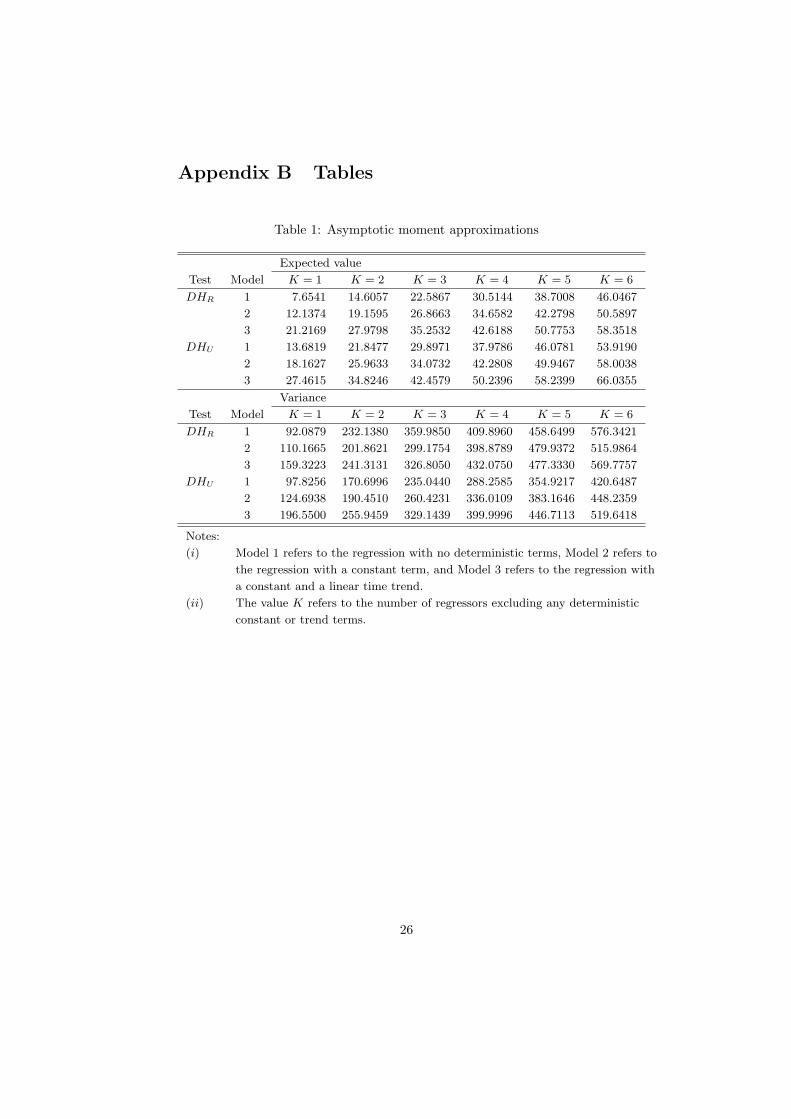
Approximations of the moments may be obtained by means of Monte Carlosimulations. In this paper, we simulate both finite and asymptotic moments. Inthe former case, the simulations are carried out by repeated application of thetest statistics to the DGP described in Section 3. In the latter case, the momentsare obtained on the basis of 10, 000 draws of K + 1 independent scaled randomwalks of length T = 1, 000. Using these random walks as simulated Brownianmotions, we construct approximations of the functional Ki and then computeapproximate asymptotic moments. The simulated moments are reported for upto six regressors in Table 1 of the appendix. For DHR statistic, our simulationresults indicate that the asymptotic results is borne out well in small sampleswith the asymptotic moment approximations being close to their finite samplecounterparts. For the DHU statistic, however, the results suggest that the finitesample moments sometimes can be far away from their theoretical values. Toaccount for such discrepancies, we estimate response surface regressions.
The estimation proceeds as follows. For each combination of K, T and N ,we generate 1, 000 test statistics according to the DGP given by (7). For theDHR statistic, T ∈ 50, 60, 70, 80, 100, 200 and N ∈ 5, 10, 15, 20, whereas,for the DHU statistic, T ∈ 50, 60, 70, 80, 100, 200, 500, 1000 and N = 1. Mostsamples are relatively small as these seem to provide more information aboutthe shape of the response surfaces. A few large values of T are also included,however, to ensure that the estimates of the asymptotic moments are sufficientlyaccurate. Pending on the deterministic component of (8), moments for threedifferent model specifications are extracted and stored, one with no deterministiccomponent, one with a constant, and one with a constant and a linear timetrend. We then perform 50 replications of each experiment, which means thatthe total number of observations available for each regression for the DHR andDHR statistics are 1200 and 400, respectively. Although the fit of the regressionsgenerally were quite good, the results suggest that the estimates associated withpowers of T greater than unity have a tendency of becoming explosive in caseswhere the dependent variable takes on relatively large values. To avoid this, wefit the regressions with the inverse of the simulated moments as the dependentvariable.
9
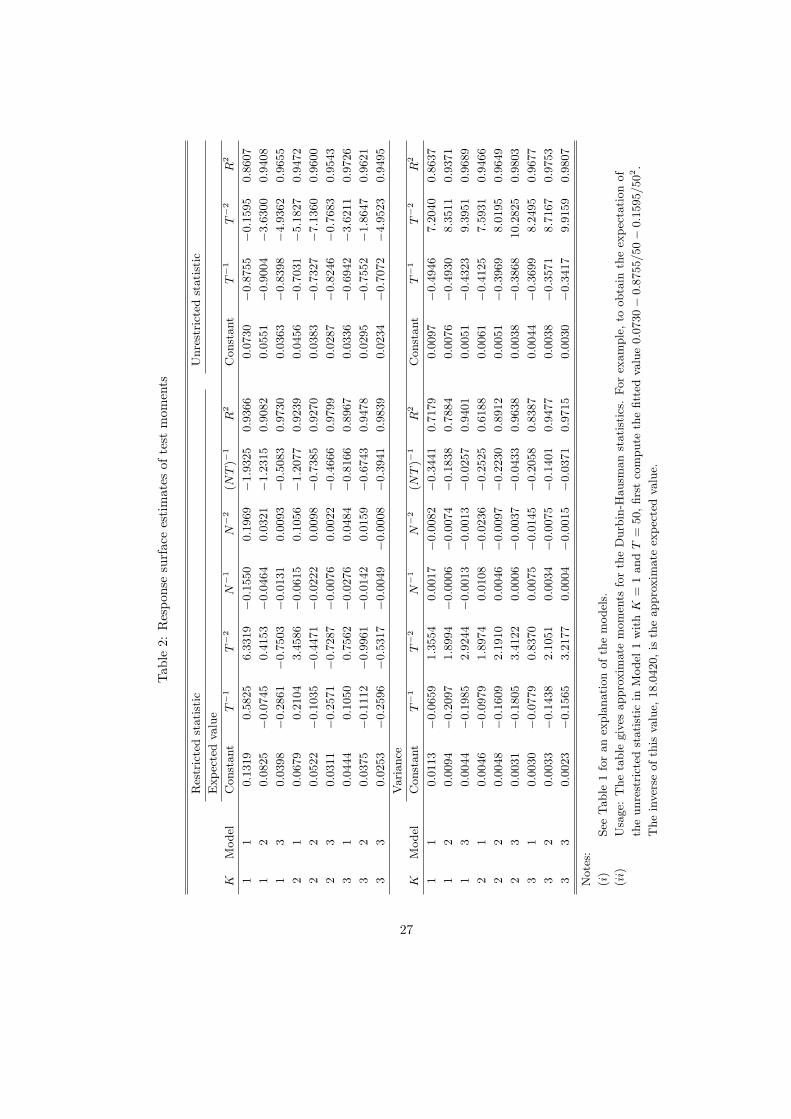
Since the regressions are heteroskedastic by construction, we use the gen-eralized method of moments estimator discussed in MacKinnon (1996). Theestimated response surface parameters for each of the experiments are reportedin Table 2. For brevity, the table only report the estimated response surfaces forup to three regressors. To test the null hypothesis of no cointegration based onthe estimated response surfaces from Table 2, one must first obtain the appro-priate moments. This is done by calculating the fitted value of the dependentvariable, which is then inverted to get the moment. For example, for the DHU
statistic in the model with no deterministic component with K = 1 and T = 50,the approximate expected value is 18.0420, which is computed as the inverseof the fitted value 0.0730 − 0.8755/50 − 0.1595/502. Based on the calculatedmoments, one then computes the value of the relevant standardized test statis-tic so that it is in the form of (10) or (11). Because both statistics diverges topositive infinity under the alternative hypothesis, the computed value shouldbe compared with the right tail of the normal distribution. If the computedvalue is greater than the appropriate right tail critical value, we reject the nullhypothesis.
5 Monte Carlo simulations
In this section, we compare and evaluate the small-sample properties of theDurbin-Hausman test statistics relative to that of eight other residual-basedtests for cointegration recently proposed by Pedroni (1999, 2004). For thispurpose, a small set of Monte Carlo experiment were conducted with the DGPtailored to reflect the most relevant features for the long-run Fisher hypothesis.In particular, we assume that the regression is fitted with a constant term onlyand that there is a single regressor in which case the DGP may be written as
rit = αi + βipit + eit,
eit = ρieit−1 + uit + θuit−1,
where (uit,∆pit)′ ∼ N(0, V ) and V is a symmetric matrix with V11 = V22 = 1and V12 = V21. For each experiment, we generate 1, 000 panels with N ∈10, 20 individual and T ∈ 50, 100 + 50 time series observations. The first50 observations for each cross-section is then disregarded in order to attenuatethe effect of the initial value. The DGP is parameterized as follows. The au-toregressive parameter ρi determines whether the null hypothesis it true or not.Under the null hypothesis, we set ρi = 1 for all i, while, under the alternativehypothesis, ρi < 1. Specifically, for the restricted test, ρi = ρ for all i, whereas,for the unrestricted test, the fraction of spurious individuals is set equal to 0.1.The regression parameters αi and βi are both allowed to vary and are drawnfrom U(0.4, 1.2). The remaining parameters θ, δ and V12 introduce nuisancein the DGP. First, a nonzero value on θ imply that eit will have a first ordermoving average component. Second, the degree of exogeneity in the DGP is
10
governed by V12. The regressor is strictly exogenous if V12 = 0, while it isweakly exogenous if V12 = 0.4. All computations was performed in GAUSS.
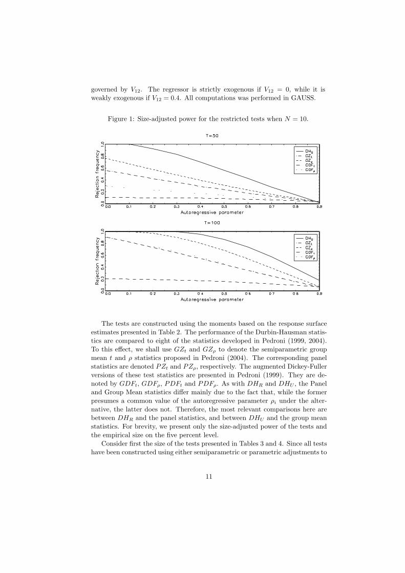
Figure 1: Size-adjusted power for the restricted tests when N = 10.
The tests are constructed using the moments based on the response surfaceestimates presented in Table 2. The performance of the Durbin-Hausman statis-tics are compared to eight of the statistics developed in Pedroni (1999, 2004).To this effect, we shall use GZt and GZρ to denote the semiparametric groupmean t and ρ statistics proposed in Pedroni (2004). The corresponding panelstatistics are denoted PZt and PZρ, respectively. The augmented Dickey-Fullerversions of these test statistics are presented in Pedroni (1999). They are de-noted by GDFt, GDFρ, PDFt and PDFρ. As with DHR and DHU , the Paneland Group Mean statistics differ mainly due to the fact that, while the formerpresumes a common value of the autoregressive parameter ρi under the alter-native, the latter does not. Therefore, the most relevant comparisons here arebetween DHR and the panel statistics, and between DHU and the group meanstatistics. For brevity, we present only the size-adjusted power of the tests andthe empirical size on the five percent level.
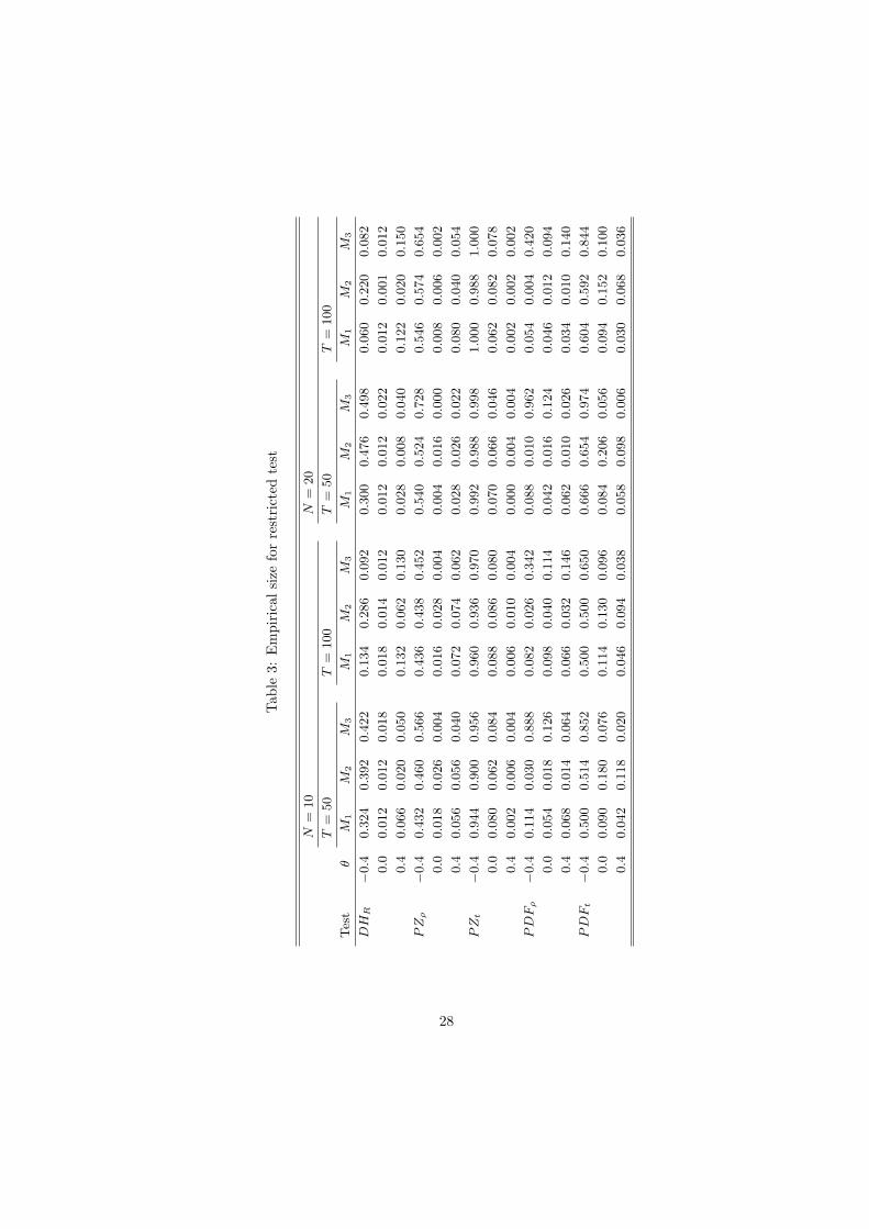
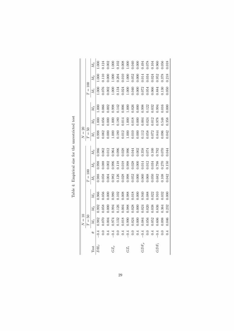
Consider first the size of the tests presented in Tables 3 and 4. Since all testshave been constructed using either semiparametric or parametric adjustments to
11
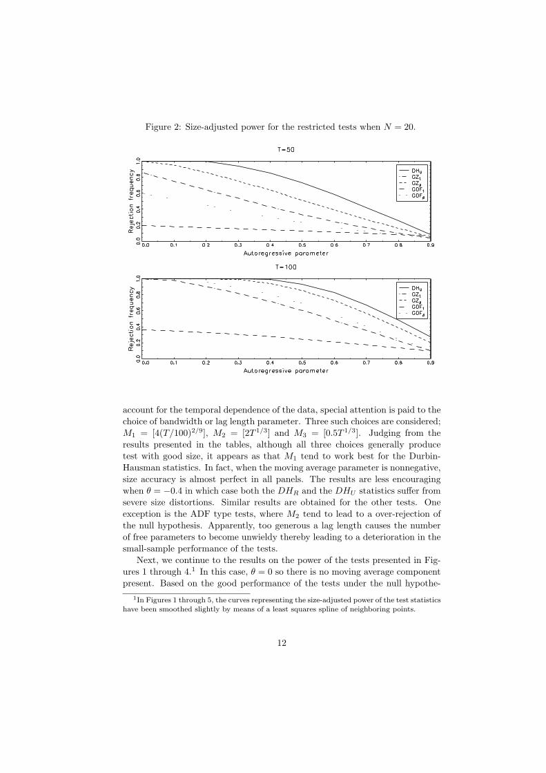
Figure 2: Size-adjusted power for the restricted tests when N = 20.
account for the temporal dependence of the data, special attention is paid to thechoice of bandwidth or lag length parameter. Three such choices are considered;M1 = [4(T/100)2/9], M2 = [2T 1/3] and M3 = [0.5T 1/3]. Judging from theresults presented in the tables, although all three choices generally producetest with good size, it appears as that M1 tend to work best for the Durbin-Hausman statistics. In fact, when the moving average parameter is nonnegative,size accuracy is almost perfect in all panels. The results are less encouragingwhen θ = −0.4 in which case both the DHR and the DHU statistics suffer fromsevere size distortions. Similar results are obtained for the other tests. Oneexception is the ADF type tests, where M2 tend to lead to a over-rejection ofthe null hypothesis. Apparently, too generous a lag length causes the numberof free parameters to become unwieldy thereby leading to a deterioration in thesmall-sample performance of the tests.
Next, we continue to the results on the power of the tests presented in Fig-ures 1 through 4.1 In this case, θ = 0 so there is no moving average componentpresent. Based on the good performance of the tests under the null hypothe-
1In Figures 1 through 5, the curves representing the size-adjusted power of the test statisticshave been smoothed slightly by means of a least squares spline of neighboring points.
12
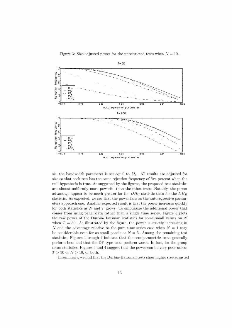
Figure 3: Size-adjusted power for the unrestricted tests when N = 10.
sis, the bandwidth parameter is set equal to M1. All results are adjusted forsize so that each test has the same rejection frequency of five percent when thenull hypothesis is true. As suggested by the figures, the proposed test statisticsare almost uniformly more powerful than the other tests. Notably, the poweradvantage appear to be much greater for the DHU statistic than for the DHR
statistic. As expected, we see that the power falls as the autoregressive param-eters approach one. Another expected result is that the power increases quicklyfor both statistics as N and T grows. To emphasize the additional power thatcomes from using panel data rather than a single time series, Figure 5 plotsthe raw power of the Durbin-Hausman statistics for some small values on N
when T = 50. As illustrated by the figure, the power is strictly increasing inN and the advantage relative to the pure time series case when N = 1 maybe considerable even for as small panels as N = 5. Among the remaining teststatistics, Figures 1 trough 4 indicate that the semiparametric tests generallyperform best and that the DF type tests perform worst. In fact, for the groupmean statistics, Figures 3 and 4 suggest that the power can be very poor unlessT > 50 or N > 10, or both.
In summary, we find that the Durbin-Hausman tests show higher size-adjusted
13
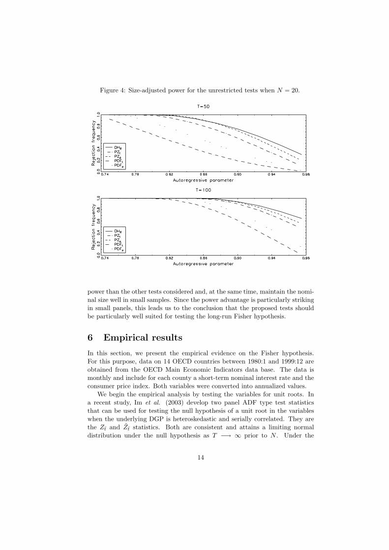
Figure 4: Size-adjusted power for the unrestricted tests when N = 20.
power than the other tests considered and, at the same time, maintain the nomi-nal size well in small samples. Since the power advantage is particularly strikingin small panels, this leads us to the conclusion that the proposed tests shouldbe particularly well suited for testing the long-run Fisher hypothesis.
6 Empirical results
In this section, we present the empirical evidence on the Fisher hypothesis.For this purpose, data on 14 OECD countries between 1980:1 and 1999:12 areobtained from the OECD Main Economic Indicators data base. The data ismonthly and include for each county a short-term nominal interest rate and theconsumer price index. Both variables were converted into annualized values.
We begin the empirical analysis by testing the variables for unit roots. Ina recent study, Im et al. (2003) develop two panel ADF type test statisticsthat can be used for testing the null hypothesis of a unit root in the variableswhen the underlying DGP is heteroskedastic and serially correlated. They arethe Zt and Zt statistics. Both are consistent and attains a limiting normaldistribution under the null hypothesis as T −→ ∞ prior to N . Under the
14
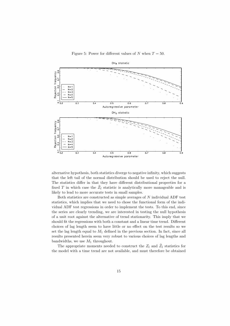
Figure 5: Power for different values of N when T = 50.
alternative hypothesis, both statistics diverge to negative infinity, which suggeststhat the left tail of the normal distribution should be used to reject the null.The statistics differ in that they have different distributional properties for afixed T in which case the Zt statistic is analytically more manageable and islikely to lead to more accurate tests in small samples.
Both statistics are constructed as simple averages of N individual ADF teststatistics, which implies that we need to chose the functional form of the indi-vidual ADF test regressions in order to implement the tests. To this end, sincethe series are clearly trending, we are interested in testing the null hypothesisof a unit root against the alternative of trend stationarity. This imply that weshould fit the regressions with both a constant and a linear time trend. Differentchoices of lag length seem to have little or no effect on the test results so weset the lag length equal to M1 defined in the previous section. In fact, since allresults presented herein seem very robust to various choices of lag lengths andbandwidths, we use M1 throughout.
The appropriate moments needed to construct the Zt and Zt statistics forthe model with a time trend are not available, and must therefore be obtained
15
by means of Monte Carlo simulation.2 As described in Section 4, this calls foran evaluation of the intermediate limiting distribution of the tests, which is theconventional Dickey-Fuller distribution defined in e.g. Im et al. (2003). For thispurpose, we make 10, 000 draws of a single random walk of length T = 1, 000,which is then used to compute the moments. The simulated expectation andvariance are −2.2208 and 0.5785, respectively. The lower tenth and fifth per-centiles of the Dickey-Fuller distribution is also simulated in order to implementthe tests on an individual basis. The simulated ten and five percent criticalvalues are −3.1476 and −3.4798, respectively.
The individual Zt and Zt statistics, abbreviated tiT and tiT , are presentedin Table 5. We see that the null hypothesis of a unit root in the variables cannotbe rejected on the five percent level for any of the 14 countries.3 These resultssuggest that we also should be able to reject the stationarity hypothesis for thepanel as a whole. Indeed, the calculated values on the Zt and Zt statistics for thenominal interest rate are −0.7805 and −0.6429, respectively. The correspondingvalues for inflation are −0.9421 and −0.7938. Hence, the null cannot be rejectedindividually nor for the panel as a whole on any conventional significance level.We therefore conclude that the variables are nonstationary.
As argued in Section 2, in the presence of unit roots, the long-run Fisher hy-pothesis necessitates that inflation and the interest rate be cointegrated. There-fore, we now proceed by testing the variables for cointegration. Results for eachindividual country are presented in Table 4. The DHS statistic is the Durbin-Hausman test developed by Choi (1994), while the ADF statistic appears inPhillips and Ouliaris (1990). Consistent with the specification of the cointe-grated regression derived in Section 2, the tests are based on a regression fittedwith a constant term only.
The results reported in Table 5 suggest that the null hypothesis of no cointe-gration can be rejected on the 10 percent level for at least 10 countries, Austria,Belgium, Canada, France, Germany, Italy, Spain, Switzerland, United Kingdom,and United States. For the remaining countries, except possibly for Finland,we end up marginally accepting the null hypothesis on the 10 percent level. Itis well known, however, that univariate tests of this sort may have low power insmall samples when the variables are nearly spurious. For this reason, we nowemploy the panel Durbin-Hausman statistics developed in Section 3 and 4. Asin Section 5, we compute the statistics based on the moments calculated fromthe response surface estimates reported in Table 2. The calculated values onDHR and DHU are 4.4785 and 4.6465, respectively. Thus, compared with theright tail of the normal distribution, we reject the null on all conventional levelsof significance. Consequently, since the variables appear to be cointegrated, weconclude that there is at least a partial Fisher effect present.
2Im et al. (2003) tabulate both finite and asymptotic moments for the Zt and Zt statisticswhen the data is generated while allowing for a nonzero mean.
3On the 10 percent level, we marginally reject the null of a unit root in the rate of inflationfor the United States using the tiT statistic.
16
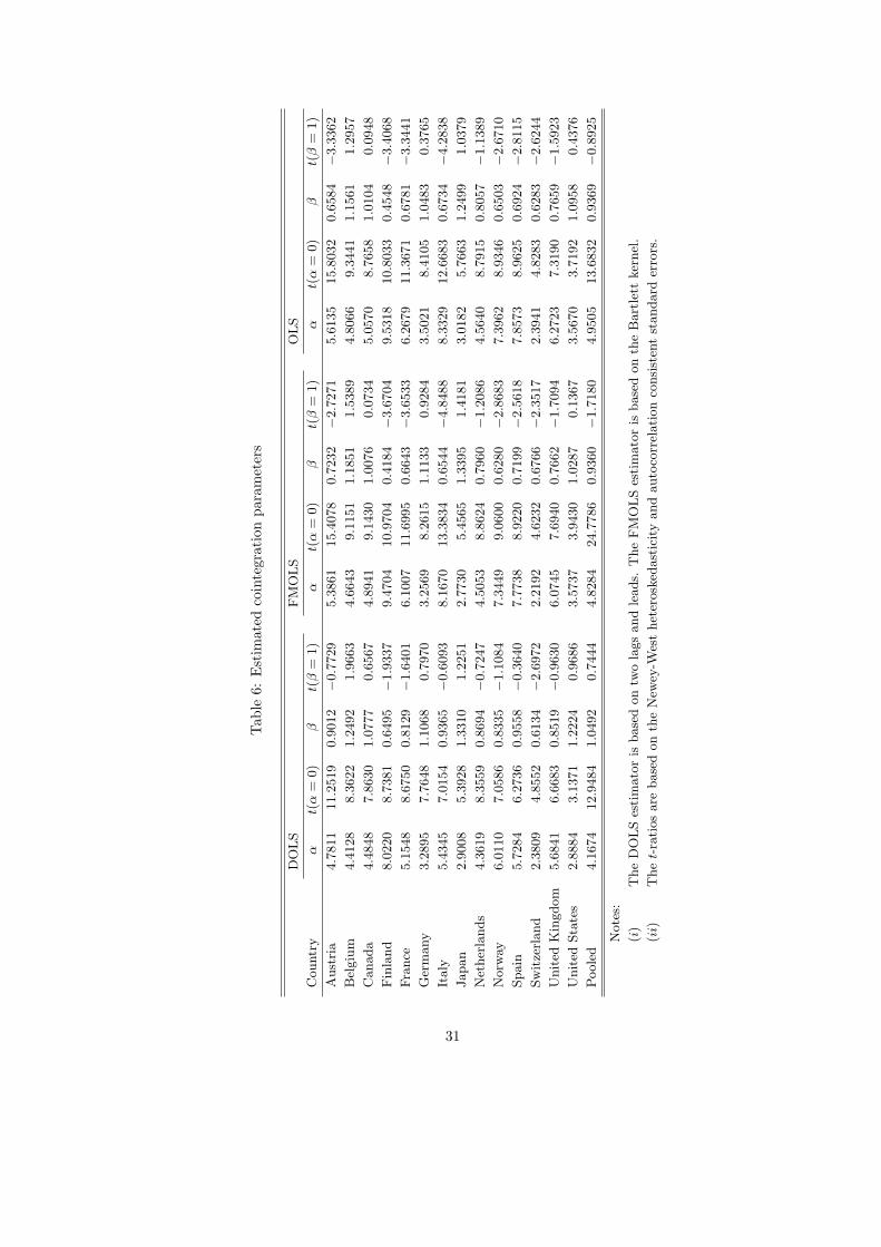
As pointed out in Section 2, the OLS estimator will be consistent under fairlygeneral conditions when applied to the cointegrated regression in (9). However,the nonzero correlation between the regression error and the first differentiatedregressor induces nuisance parameters in the asymptotic distribution of the OLSestimator, which then falls outside the local asymptotic mixture of normals fam-ily. Moreover, the use of overlapping data, where the horizon of the inflation andinterest rates are longer than the monthly observation interval, may induce serialcorrelation in the equilibrium errors. To account for both of these features, weemploy the dynamic OLS (DOLS) estimator of Stock and Watson (1993), andSaikkonen (1991) and the fully modified OLS (FMOLS) estimator of Phillipsand Hansen (1990). These estimators are asymptotically equivalent and fullyefficient in the presence of serially correlated errors and endogenous regressors.The difference between them lies in the methods undertaken in order to ensureefficiency of the cointegration parameters. Specifically, while the DOLS employsa parametric correction whereby lags and leads of the first differentiated regres-sor are introduced, the FMOLS adjusts for the temporal dependencies of thedata by directly estimating the various nuisance parameters semiparametrically.To this effect, we use two lags and leads of the first difference of inflation toconstruct the DOLS, whereas the FMOLS is based on the Bartlett kernel.
The results from the estimated cointegration parameters are reported inTable 6. We see that the estimated individual slope parameters generally lieclose to their hypothesized value of one. The range of the estimated slopes are0.6134 to 1.3310 for the DOLS, 0.4184 to 1.3394 for the FMOLS, and 0.4548to 1.2499 for the OLS. Based on the asymptotic normal distribution, we canrarely reject the null hypothesis of a unit slope parameter on the one percentlevel. The pooled estimates are reported in the last row of the table. Consistentwith the individual county regressions, we see that the pooled slopes are closeto unity and that the null hypothesis of a unit slope cannot be rejected onthe five percent level using the normal distribution for any of the estimators.These estimates should, however, be interpreted with caution as the poolabilityrestriction do not seem to be supported by the data.4
Consistent with the results of e.g. Mishkin (1992), Crowder and Hoffman(1992), and Evans and Lewis (1995), we observe some countries where the esti-mated slope is significantly less than unity. One interpretation of this finding isthat the ex ante real interest rate is subject to permanent shocks and that theseshocks are negatively correlated with the permanent shocks to inflation, which isinconsistent with the Fisher hypothesis. To appreciate this, note from (5) thatthe unit root component of the ex post real rate can be written as −(1−βi)pit.Thus, a unit positive permanent shock to inflation translate into a permanentshock in the ex post real rate of magnitude −(1−βi). Since βi < 1 in this case,
4The calculated Wald test statistics for a homogenous slope parameter are 87.0098 for theDOLS, 42.9126 for the FMOLS and 87.2586 for the OLS estimator. Under the null hypothesisof a common slope, these statistics have a limiting chi-squared distribution with 13 degrees offreedom in which case the five percent critical value is 22.3621.
17
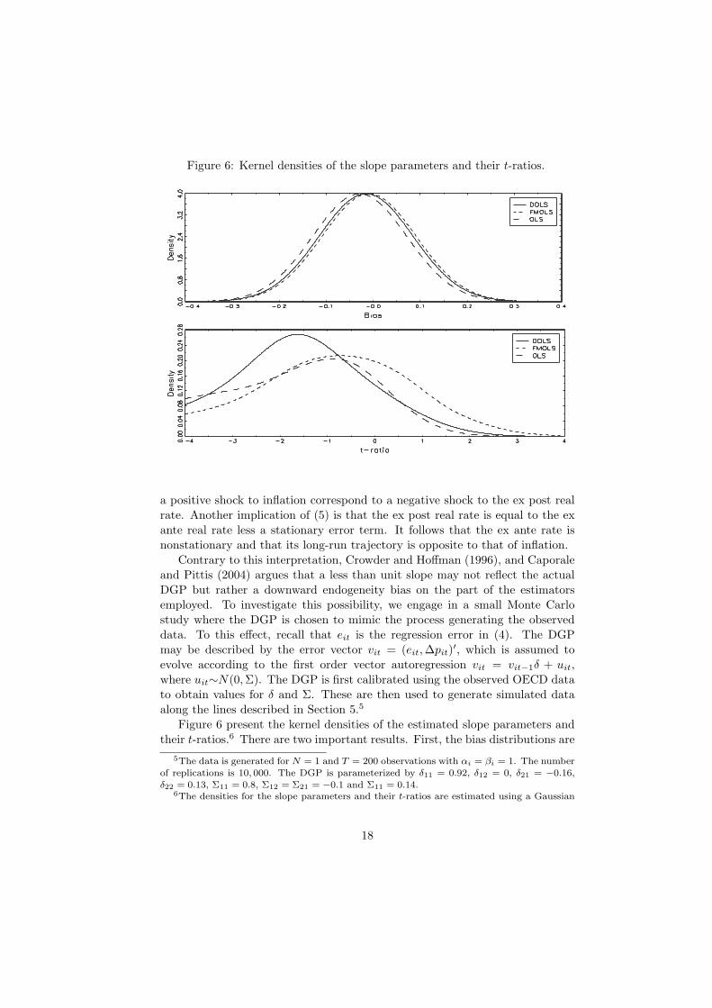
Figure 6: Kernel densities of the slope parameters and their t-ratios.
a positive shock to inflation correspond to a negative shock to the ex post realrate. Another implication of (5) is that the ex post real rate is equal to the exante real rate less a stationary error term. It follows that the ex ante rate isnonstationary and that its long-run trajectory is opposite to that of inflation.
Contrary to this interpretation, Crowder and Hoffman (1996), and Caporaleand Pittis (2004) argues that a less than unit slope may not reflect the actualDGP but rather a downward endogeneity bias on the part of the estimatorsemployed. To investigate this possibility, we engage in a small Monte Carlostudy where the DGP is chosen to mimic the process generating the observeddata. To this effect, recall that eit is the regression error in (4). The DGPmay be described by the error vector vit = (eit, ∆pit)′, which is assumed toevolve according to the first order vector autoregression vit = vit−1δ + uit,where uit∼N(0, Σ). The DGP is first calibrated using the observed OECD datato obtain values for δ and Σ. These are then used to generate simulated dataalong the lines described in Section 5.5
Figure 6 present the kernel densities of the estimated slope parameters andtheir t-ratios.6 There are two important results. First, the bias distributions are
5The data is generated for N = 1 and T = 200 observations with αi = βi = 1. The numberof replications is 10, 000. The DGP is parameterized by δ11 = 0.92, δ12 = 0, δ21 = −0.16,δ22 = 0.13, Σ11 = 0.8, Σ12 = Σ21 = −0.1 and Σ11 = 0.14.
6The densities for the slope parameters and their t-ratios are estimated using a Gaussian
18
peaked to the left of zero suggesting that the estimators are biased downwardswith the OLS estimator being the most biased. Second, the distributions ofthe t-ratios are highly non-central and shifted to the left. Notably, the meanvalues of the t-ratios are −1.2736 for the DOLS, −0.5468 for the FMOLS and−1.5202 for the OLS, which is indicative of large size distortions. Indeed, theprobability of rejecting a true null hypothesis of βi = 1 using a double-sidedtest against the normal distribution on the nominal five percent level is 0.342for the DOLS, 0.198 for the FMOLS and 0.386 for the OLS. Hence, inferencebased on the normal distribution is likely to be highly deceptive. To account forthis, we obtain the five percent critical values form the empirical distribution,which should enable valid inference. The left tail critical values for the DOLS,FMOLS and OLS estimators are −3.8392, −4.1619 and −5.5901, respectively.Based on these values, the null of a unit slope cannot be rejected for any of thecountries using the t-ratios reported in Table 6.
In summary, consistent with the results of Crowder and Hoffman (1996), andCaporale and Pittis (2004), the evidence of this section suggests that we cannotreject the full Fisher effect for any of the countries or for the panel as a whole. Totest the robustness of this conclusion, we reestimated the empirical model basedon both annual and quarterly OECD data. Some additional estimates were alsoobtained using the yield on long-term government bonds as interest rate. Forbrevity, however, we do not report these results but we briefly describe them.Regardless of sample frequency, we still find cointegration between the inflationand nominal interest rates. The full Fisher effect is also supported using theempirical critical values. The results obtained using long-term interest rates arequalitatively similar. An additional, and perhaps even more important, caveatis that all forms of cross-sectional dependency thus far has been disregarded.To this end, the next section proposes bootstrapped cointegration tests that arerobust to general forms of cross-sectional dependencies.
7 Bootstrap tests
Recall that the properties of the Durbin-Hausman test statistics rely on theassumption of cross-sectional independence. When this assumption is violated,the statistics suffer from nuisance parameter dependencies in which case theirasymptotic distributions are unknown. In our case, there are at least two reasonsfor believing that the data may not be i.i.d. cross-sectionally. First, inflationrates may be correlated across countries because of common oil price shocks.Second, nominal interest rates may be correlated across countries due to thestrong links between financial markets. Although the first type of dependencemay be accommodated by using data that has been demeaned with respect toa common time effect, the size of such tests may be quite unreliable once weallow for more general types of correlation structures. One possible response to
kernel with bandwidth parameter 0.1 and 0.6, respectively.
19
this is to follow Maddala and Wu (1999) in employing the bootstrap approach,which enables us to make accurate inference using the empirical distributionsof the test statistics.
The problem is how to generate the bootstrap distributions. To this end, wepropose generating the data nonparametrically using the sampling scheme S2
described in Li and Maddala (1996, 1997). Specifically, if the null hypothesis isspecified as ρi = 1 for all i, then this scheme suggests that the sample shouldbe generated while imposing a unit root in the equilibrium errors. Thus, thebootstrap sample e∗it is generated as
e∗it = e∗it−1 + u∗it,
where u∗it is the bootstrap sample from the centered residual uit = uit −T−1
∑Tt=1 uit obtained by performing OLS on (9). Because the errors are cross-
sectionally correlated, however, we cannot resample uit directly. Instead, weresample vt = (u′t,∆p′t)′, where ut = (u1t, ..., uNt)′ and ∆pt = (∆p1t, ..., ∆pNt)′.By resampling the data in this way, we can preserve the cross-sectional correla-tion structure of vt. Notably, by resampling vt rather than ut, we can preserveany endogenous effects that may run across the individual regressions of thesystem. Next, we generate the bootstrap sample r∗it as
r∗it = αi + βip∗it + e∗it,
where αi and βi are the parameters from (8). For initiation of e∗it and p∗it, we usethe value zero. Once the sample r∗it and p∗it has been obtained, the bootstrappedtest statistics may be readily computed. This procedure is then repeated a largenumber of times, which gives us the empirical distributions of the statistics.
The five percent critical values for the DHR and DHU statistics obtainedusing 1, 000 bootstrap replications are 19.922 and 4.435, respectively. Thus,based on the DHU statistic, we reject the null hypothesis of no cointegrationon the five percent level using the bootstrapped distribution. In contrast, wecannot reject the null on the five percent level using the DHR statistic. This isnot unexpected, however, given the results on the individual cointegration tests,which suggest that the homogenous alternative may be too restrictive in thiscase. Generally speaking, these empirical findings seem to confirm our simula-tion results, which suggest that the DHR statistic suffers from substantial sizedistortions when the errors are cross-sectionally correlated. The DHU statisticalso suffers from size distortions but not nearly as severe as those for the DHR
statistic. In fact, the DHU statistic appears to be rather robust against smallto moderate degrees of cross-section dependence. The bootstrap approach elim-inates these distortions and leads to tests with good size properties, althoughboth tests tend to be somewhat under-sized.
20
8 Conclusions
Recent empirical studies suggest that the Fisher hypothesis, stating that infla-tion and nominal interest rates should cointegrate with a unit parameter oninflation, do not hold, a finding at odds with many theoretical models. Thispaper argues that these results can be explained in part by the low power in-herent in univariate cointegration tests and that the use of panel data shouldgenerate more powerful tests. Therefore, in this paper we investigate the Fisherhypothesis using a panel of monthly data covering the period 1980:1 to 1999:12on 14 OECD countries. In doing so, we propose two new residual-based testsfor the null hypothesis of no cointegration. The tests are based on the Durbin-Hausman principle whereby two estimators of a unit root in the residuals of acointegrated regression are compared. Both estimators are consistent under thenull hypothesis but only one retains the property of consistency under the alter-native. Using sequential limit arguments, it is shown that the test statistics arefree of nuisance parameters and that they have a limiting normal distributionunder the null hypothesis. Results from a small Monte Carlo study suggest thatthe proposed tests have greater power than other popular residual-based testsis samples comparable with ours. In our empirical analysis, contrary to muchof the earlier literature, we find evidence in favor of the Fisher hypothesis.
21
Appendix A Mathematical proofs
In this appendix, we derive the limiting distributions of the Durbin-Hausmantest statistics under the null hypothesis of no cointegration. Unless otherwisestated, the limit arguments are taken passing T −→ ∞ with N held fixed. Forillustrative purposes, we shall focus on the simple case when the regression (11)is fitted without any deterministic components.
Proof of Theorem 1. To prove the limiting distribution for the restrictedDurbun-Hausman test statistic, we make the assumption that ρi = ρ for all i.Thus, since ρ = 1 under the null hypothesis, we may write
T ρ =(T−2E22
)−1T−1E12 = T +
(T−2E22
)−1T−1E23, (A1)
T ρ =(T−2E12
)−1T−1E22 = T +
(T−2E12
)−1T−1E13. (A2)
The estimated OLS regression (11) with no deterministic component may beexpressed as λ′izit = eit, where λi = (1,−βi)′. Furthermore, by Theorem 2 ofPhillips (1986), we obtain the limit of λi as
λi ⇒ λi = (1,−ai21A−1i22)
′,
where
Ai =∫ 1
0
BiB′i =
(ai11 ai21
ai21 Ai22
).
Combining the results, it follows that
T−2Ei11 ⇒ λ′iAiλi = ω2i1.2
∫ 1
0
Q2i , (A3)
Moreover, by Theorem 2.6 of Phillips (1988), we obtain
T−1Ei23 = λ′i
(T−1
T∑t=2
vitzit−1
)λi ⇒ λ′i
(∫ 1
0
BidBi + Γi
)λi. (A4)
From (A3) and (A4), we deduce
T−2Ei12 = T−2Ei11 + T−2Ei23 = T−2Ei11 + op(1) ⇒ λ′iAiλi, (A5)
T−1Ei13 = T−1Ei23 + T−1Ei11
= λ′i
(T−1
T∑t=2
vitzit−1 + T−1T∑
t=2
vitv′it
)λi
⇒ λ′i
(∫ 1
0
BidBi + Σi + Γi
)λi. (A6)
22
Combining (A3) through (A6), since ω2i1.2 is consistent for ω2
i1.2 under Assump-tion 2 (see, e.g. Phillips and Ouliaris, 1990), we obtain the limit of T (ρ−1) andT (ρ− 1) as follows
T (ρ− 1) ⇒(
N∑
i=1
ω−2i1.2λ
′iAiλi
)−1 N∑
i=1
ω−2i1.2λ
′i
(∫ 1
0
BidBi + Γi
)λi,
T (ρ− 1) ⇒(
N∑
i=1
ω−2i1.2λ
′iAiλi
)−1 N∑
i=1
ω−2i1.2λ
′i
(∫ 1
0
BidBi + Σi + Γi
)λi.
It follows that
T (ρ− ρ) =
(T−2
N∑
i=1
ω−2i1.2Ei12
)−1
T−1N∑
i=1
ω−2i1.2Ei13
−(
T−2N∑
i=1
ω−2i1.2Ei22
)−1
T−1N∑
i=1
ω−2i1.2Ei23
⇒(
N∑
i=1
ω−2i1.2λ
′iAiλi
)−1 N∑
i=1
ω−2i1.2λ
′iΣiλi
=
(N∑
i=1
∫ 1
0
Q2i
)−1 N∑
i=1
ω−2i1.2λ
′iΣiλi. (A7)
Next, consider γ0 and σ2. For simplicity, write R0 =∑N
i=1 ω−2i1.2γi0 and R1 =∑N
i=1 ω−2i1.2σ
2i . From Lemma 2.2 of Phillips and Ouliaris (1990), we have λ′iΩiλi =
ω2i1.2V
′i Vi. Thus, using the same arguments as Choi (1994), it is possible to show
γ0 = N−1R0 ⇒ N−1N∑
i=1
ω−2i1.2λ
′iΣiλi, (A8)
σ2 = N−1R1 ⇒ N−1N∑
i=1
ω−2i1.2λ
′iΩiλi = N−1
N∑
i=1
V ′i Vi. (A9)
Using the results in (A3), (A7) and (A8), we have
R2 ≡ (N−1R0
)2(T (ρ− ρ))−2
(T−2
N∑
i=1
ω−2i1.2Ei22
)−2
⇒ N−2N∑
i=1
∫ 1
0
Q2i . (A10)
This, together with (A9), imply
DHR = σ2γ−20 (ρ− ρ)2
N∑
i=1
ω−2i1.2Ei22
23
= N−1R1R−12
⇒(
N−1N∑
i=1
V ′i Vi
)(N−2
N∑
i=1
∫ 1
0
Q2i
)−1
. (A11)
This shows that the limiting distribution of DHR is free of nuisance parametersunder the null. Therefore, because the limiting distributions passing T −→ ∞is i.i.d. over the cross-section, we deduce that E(Ki) = Θ for all i. The varianceof Ki may be decomposed as
Σ =
Σ11 Σ12 Σ13
Σ12 Σ22 Σ23
Σ13 Σ23 Σ33
and Σ =
(Σ11 Σ12
Σ12 Σ22
).
To derive the limiting distributions of the test statistic, we shall make use ofthe Delta method, which provides the limiting distribution for continuouslydifferentiable transformations of i.i.d. vector sequences. In so doing, rewrite thestatistic as
N−1/2DHR −N1/2Θ1Θ−12 = N1/2
(N−1R1 −Θ1
) (N−1R2
)−1
+ N1/2Θ1
((N−1R2
)−1 −Θ−12
). (A12)
The terms appearing in (A12) with normalizing order N−1 converge in prob-ability to the means of the corresponding random variables by virtue of a lawof large numbers as T −→ ∞ and then N −→ ∞. Hence, N−1R1
p→ Θ1 andN−1R2
p→ Θ2. Moreover, by direct application of the Lindberg-Levy centrallimit theorem, N1/2
(N−1R1 −Θ1
) ⇒ N(0,Σ11) as T −→ ∞ prior to N . Theremaining expression involves a continuously differentiable transformation ofi.i.d. random variables. Thus, by the Delta method, as T −→∞ prior to N
N1/2((
N−1R2
)−1 −Θ−12
)⇒ N(0, Θ−4
2 Σ22). (A13)
This suggests that the limit of N−1/2DHR −N1/2Θ1Θ−12 may be written as
N−1/2DHR −N1/2Θ1Θ−12 ⇒ Θ−1
2 N(0, Σ11)−Θ1Θ−22 N(0, Σ22). (A14)
It follows that N−1/2DHR −N1/2Θ1Θ−12 is mean zero with the variance given
by Θ−22 Σ11 + Θ2
1Θ−42 Σ22 − 2Θ1Θ−3
2 Σ12. This completes the first part of theproof.
Consider next the limiting distribution of the DHU statistic. In this case,ρi need not take on a common value in which case the OLS and pseudo IVestimators may be rewritten as
T ρi =(T−2Ei22
)−1T−1Ei12 = T +
(T−2Ei22
)−1T−1Ei23, (A15)
T ρi =(T−2Ei12
)−1T−1Ei11 = T +
(T−2Ei12
)−1T−1Ei13. (A16)
24
Using (A3) through (A6) it follows that
T (ρi − ρi) ⇒ λ′iΣiλi (λ′iAiλi)−1
. (A17)
Moreover, from (A8) and (A9), we infer that γi0 ⇒ λ′iΣiλi and σ2i ⇒ λ′iΩiλi.
Together, these results indicate
DHU =N∑
i=1
σ2i γ−2
i0 (ρi − ρi)2Ei22
=N∑
i=1
σ2i γ−2
i0 (T (ρi − ρi))2(T−2Ei22
)
⇒N∑
i=1
λ′iΩiλi (λ′iAiλi)−1 =
N∑
i=1
V ′i Vi
(∫ 1
0
Q2i
)−1
. (A18)
Next, let Ri = σ2i γ−2
i0 (T (ρi − ρi))2 (
T−2Ei22
)and rewrite the statistic as follows
N−1/2DHU −N1/2Θ3 = N1/2
(N−1
N∑
i=1
Ri −Θ33
). (A19)
Hence, by the Lindberg-Levy central limit theorem, N−1/2DHU − N1/2Θ3 ⇒N(0, Σ33) as T −→∞ prior to N . This establishes the second part of the proof.¥
25
Appendix B Tables
Table 1: Asymptotic moment approximations
Expected value
Test Model K = 1 K = 2 K = 3 K = 4 K = 5 K = 6
DHR 1 7.6541 14.6057 22.5867 30.5144 38.7008 46.0467
2 12.1374 19.1595 26.8663 34.6582 42.2798 50.5897
3 21.2169 27.9798 35.2532 42.6188 50.7753 58.3518
DHU 1 13.6819 21.8477 29.8971 37.9786 46.0781 53.9190
2 18.1627 25.9633 34.0732 42.2808 49.9467 58.0038
3 27.4615 34.8246 42.4579 50.2396 58.2399 66.0355
Variance
Test Model K = 1 K = 2 K = 3 K = 4 K = 5 K = 6
DHR 1 92.0879 232.1380 359.9850 409.8960 458.6499 576.3421
2 110.1665 201.8621 299.1754 398.8789 479.9372 515.9864
3 159.3223 241.3131 326.8050 432.0750 477.3330 569.7757
DHU 1 97.8256 170.6996 235.0440 288.2585 354.9217 420.6487
2 124.6938 190.4510 260.4231 336.0109 383.1646 448.2359
3 196.5500 255.9459 329.1439 399.9996 446.7113 519.6418
Notes:
(i) Model 1 refers to the regression with no deterministic terms, Model 2 refers to
the regression with a constant term, and Model 3 refers to the regression with
a constant and a linear time trend.
(ii) The value K refers to the number of regressors excluding any deterministic
constant or trend terms.
26
Tab
le2:
Res
pons
esu
rfac
ees
tim
ates
ofte
stm
omen
ts
Res
tric
ted
stati
stic
Unre
stri
cted
stati
stic
Expec
ted
valu
e
KM
odel
Const
ant
T−
1T−
2N−
1N−
2(N
T)−
1R
2C
onst
ant
T−
1T−
2R
2
11
0.1
319
0.5
825
6.3
319
−0.1
550
0.1
969
−1.9
325
0.9
366
0.0
730
−0.8
755
−0.1
595
0.8
607
12
0.0
825
−0.0
745
0.4
153
−0.0
464
0.0
321
−1.2
315
0.9
082
0.0
551
−0.9
004
−3.6
300
0.9
408
13
0.0
398
−0.2
861
−0.7
503
−0.0
131
0.0
093
−0.5
083
0.9
730
0.0
363
−0.8
398
−4.9
362
0.9
655
21
0.0
679
0.2
104
3.4
586
−0.0
615
0.1
056
−1.2
077
0.9
239
0.0
456
−0.7
031
−5.1
827
0.9
472
22
0.0
522
−0.1
035
−0.4
471
−0.0
222
0.0
098
−0.7
385
0.9
270
0.0
383
−0.7
327
−7.1
360
0.9
600
23
0.0
311
−0.2
571
−0.7
287
−0.0
076
0.0
022
−0.4
666
0.9
799
0.0
287
−0.8
246
−0.7
683
0.9
543
31
0.0
444
0.1
050
0.7
562
−0.0
276
0.0
484
−0.8
166
0.8
967
0.0
336
−0.6
942
−3.6
211
0.9
726
32
0.0
375
−0.1
112
−0.9
961
−0.0
142
0.0
159
−0.6
743
0.9
478
0.0
295
−0.7
552
−1.8
647
0.9
621
33
0.0
253
−0.2
596
−0.5
317
−0.0
049
−0.0
008
−0.3
941
0.9
839
0.0
234
−0.7
072
−4.9
523
0.9
495
Vari
ance
KM
odel
Const
ant
T−
1T−
2N−
1N−
2(N
T)−
1R
2C
onst
ant
T−
1T−
2R
2
11
0.0
113
−0.0
659
1.3
554
0.0
017
−0.0
082
−0.3
441
0.7
179
0.0
097
−0.4
946
7.2
040
0.8
637
12
0.0
094
−0.2
097
1.8
994
−0.0
006
−0.0
074
−0.1
838
0.7
884
0.0
076
−0.4
930
8.3
511
0.9
371
13
0.0
044
−0.1
985
2.9
244
−0.0
013
−0.0
013
−0.0
257
0.9
401
0.0
051
−0.4
323
9.3
951
0.9
689
21
0.0
046
−0.0
979
1.8
974
0.0
108
−0.0
236
−0.2
525
0.6
188
0.0
061
−0.4
125
7.5
931
0.9
466
22
0.0
048
−0.1
609
2.1
910
0.0
046
−0.0
097
−0.2
230
0.8
912
0.0
051
−0.3
969
8.0
195
0.9
649
23
0.0
031
−0.1
805
3.4
122
0.0
006
−0.0
037
−0.0
433
0.9
638
0.0
038
−0.3
868
10.2
825
0.9
803
31
0.0
030
−0.0
779
0.8
370
0.0
075
−0.0
145
−0.2
058
0.8
387
0.0
044
−0.3
699
8.2
495
0.9
677
32
0.0
033
−0.1
438
2.1
051
0.0
034
−0.0
075
−0.1
401
0.9
477
0.0
038
−0.3
571
8.7
167
0.9
753
33
0.0
023
−0.1
565
3.2
177
0.0
004
−0.0
015
−0.0
371
0.9
715
0.0
030
−0.3
417
9.9
159
0.9
807
Note
s:
(i)
See
Table
1fo
ran
expla
nati
on
ofth
em
odel
s.
(ii)
Usa
ge:
The
table
giv
esappro
xim
ate
mom
ents
for
the
Durb
in-H
ausm
an
stati
stic
s.For
exam
ple
,to
obta
inth
eex
pec
tati
on
of
the
unre
stri
cted
stati
stic
inM
odel
1w
ith
K=
1and
T=
50,firs
tco
mpute
the
fitt
edva
lue
0.0
730−
0.8
755/50−
0.1
595/502.
The
inver
seofth
isva
lue,
18.0
420,is
the
appro
xim
ate
expec
ted
valu
e.
27
Tab
le3:
Em
piri
calsi
zefo
rre
stri
cted
test
N=
10
N=
20
T=
50
T=
100
T=
50
T=
100
Tes
tθ
M1
M2
M3
M1
M2
M3
M1
M2
M3
M1
M2
M3
DH
R−0
.40.3
24
0.3
92
0.4
22
0.1
34
0.2
86
0.0
92
0.3
00
0.4
76
0.4
98
0.0
60
0.2
20
0.0
82
0.0
0.0
12
0.0
12
0.0
18
0.0
18
0.0
14
0.0
12
0.0
12
0.0
12
0.0
22
0.0
12
0.0
01
0.0
12
0.4
0.0
66
0.0
20
0.0
50
0.1
32
0.0
62
0.1
30
0.0
28
0.0
08
0.0
40
0.1
22
0.0
20
0.1
50
PZ
ρ−0
.40.4
32
0.4
60
0.5
66
0.4
36
0.4
38
0.4
52
0.5
40
0.5
24
0.7
28
0.5
46
0.5
74
0.6
54
0.0
0.0
18
0.0
26
0.0
04
0.0
16
0.0
28
0.0
04
0.0
04
0.0
16
0.0
00
0.0
08
0.0
06
0.0
02
0.4
0.0
56
0.0
56
0.0
40
0.0
72
0.0
74
0.0
62
0.0
28
0.0
26
0.0
22
0.0
80
0.0
40
0.0
54
PZ
t−0
.40.9
44
0.9
00
0.9
56
0.9
60
0.9
36
0.9
70
0.9
92
0.9
88
0.9
98
1.0
00
0.9
88
1.0
00
0.0
0.0
80
0.0
62
0.0
84
0.0
88
0.0
86
0.0
80
0.0
70
0.0
66
0.0
46
0.0
62
0.0
82
0.0
78
0.4
0.0
02
0.0
06
0.0
04
0.0
06
0.0
10
0.0
04
0.0
00
0.0
04
0.0
04
0.0
02
0.0
02
0.0
02
PD
Fρ
−0.4
0.1
14
0.0
30
0.8
88
0.0
82
0.0
26
0.3
42
0.0
88
0.0
10
0.9
62
0.0
54
0.0
04
0.4
20
0.0
0.0
54
0.0
18
0.1
26
0.0
98
0.0
40
0.1
14
0.0
42
0.0
16
0.1
24
0.0
46
0.0
12
0.0
94
0.4
0.0
68
0.0
14
0.0
64
0.0
66
0.0
32
0.1
46
0.0
62
0.0
10
0.0
26
0.0
34
0.0
10
0.1
40
PD
Ft
−0.4
0.5
00
0.5
14
0.8
52
0.5
00
0.5
00
0.6
50
0.6
66
0.6
54
0.9
74
0.6
04
0.5
92
0.8
44
0.0
0.0
90
0.1
80
0.0
76
0.1
14
0.1
30
0.0
96
0.0
84
0.2
06
0.0
56
0.0
94
0.1
52
0.1
00
0.4
0.0
42
0.1
18
0.0
20
0.0
46
0.0
94
0.0
38
0.0
58
0.0
98
0.0
06
0.0
30
0.0
68
0.0
36
28
Tab
le4:
Em
piri
calsi
zefo
rth
eun
rest
rict
edte
st
N=
10
N=
20
T=
50
T=
100
T=
50
T=
100
Tes
tθ
M1
M2
M3
M1
M2
M3
M1
M2
M3
M1
M2
M3
DH
U−0
.40.9
82
0.9
92
0.9
66
0.9
88
0.9
98
0.9
86
0.9
98
1.0
00
1.0
00
1.0
00
1.0
00
1.0
00
0.0
0.0
70
0.0
58
0.0
56
0.0
58
0.0
88
0.0
62
0.0
62
0.0
56
0.0
66
0.0
76
0.1
10
0.1
24
0.4
0.0
04
0.0
00
0.0
00
0.0
04
0.0
02
0.0
12
0.0
00
0.0
00
0.0
02
0.0
02
0.0
00
0.0
02
GZ
ρ−0
.40.9
74
0.9
94
0.9
80
0.9
82
0.9
96
0.9
64
1.0
00
1.0
00
0.9
98
1.0
00
1.0
00
1.0
00
0.0
0.1
32
0.1
26
0.1
02
0.1
26
0.1
18
0.0
96
0.1
80
0.1
80
0.1
42
0.1
34
0.2
04
0.1
02
0.4
0.0
18
0.0
04
0.0
08
0.0
28
0.0
18
0.0
28
0.0
12
0.0
14
0.0
06
0.0
24
0.0
10
0.0
08
GZ
t−0
.40.9
90
0.9
88
0.9
88
0.9
98
0.9
98
0.9
96
1.0
00
1.0
00
1.0
00
1.0
00
1.0
00
1.0
00
0.0
0.0
24
0.0
28
0.0
18
0.0
52
0.0
28
0.0
44
0.0
10
0.0
18
0.0
26
0.0
40
0.0
52
0.0
40
0.4
0.0
00
0.0
00
0.0
00
0.0
00
0.0
00
0.0
02
0.0
00
0.0
00
0.0
00
0.0
00
0.0
00
0.0
00
GD
Fρ
−0.4
0.0
84
0.0
24
0.9
40
0.0
60
0.0
14
0.3
58
0.1
12
0.0
04
0.9
98
0.0
72
0.0
14
0.4
94
0.0
0.0
56
0.0
20
0.0
88
0.0
68
0.0
12
0.0
74
0.0
58
0.0
24
0.1
22
0.0
54
0.0
34
0.0
78
0.4
0.0
52
0.0
38
0.0
22
0.0
50
0.0
34
0.1
00
0.0
72
0.0
12
0.0
32
0.0
66
0.0
24
0.1
04
GD
Ft
−0.4
0.6
06
0.8
36
0.9
10
0.6
82
0.7
98
0.7
92
0.8
44
0.9
78
0.9
94
0.8
84
0.9
52
0.9
60
0.0
0.0
98
0.3
64
0.0
32
0.1
08
0.2
70
0.0
70
0.0
96
0.5
48
0.0
16
0.1
30
0.3
78
0.0
56
0.4
0.0
46
0.2
32
0.0
00
0.0
42
0.1
50
0.0
44
0.0
42
0.3
58
0.0
00
0.0
50
0.2
18
0.0
18
29
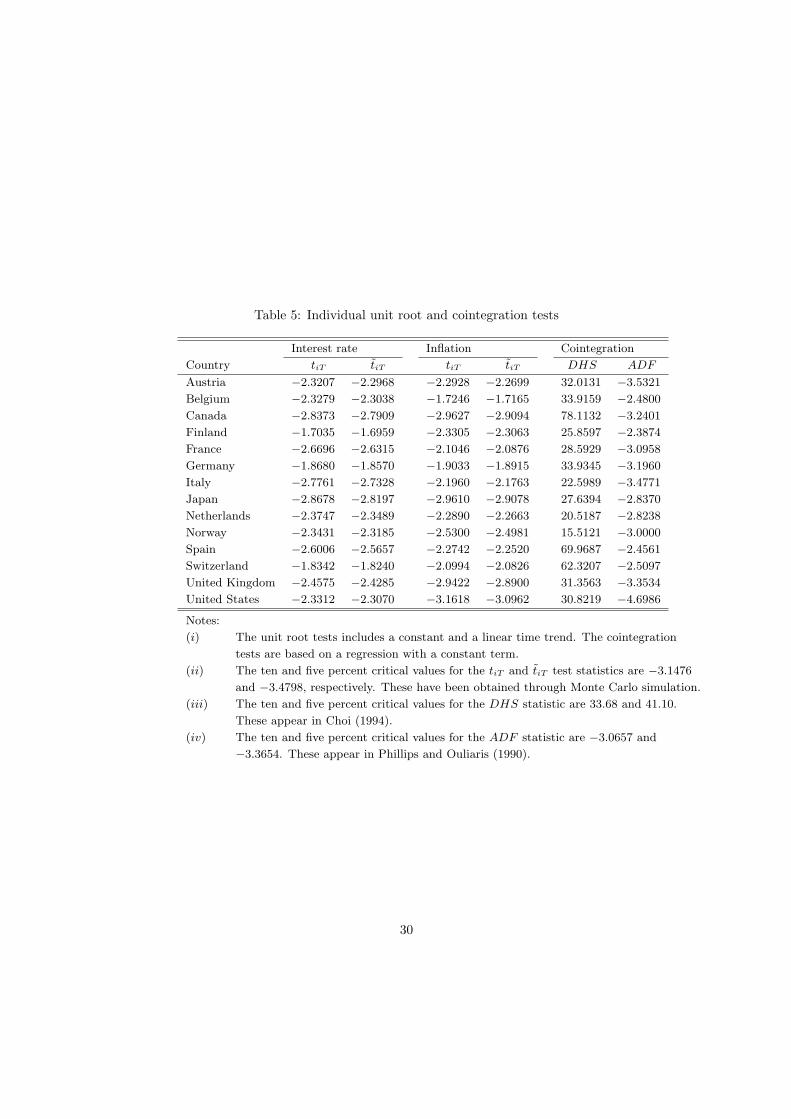
Table 5: Individual unit root and cointegration tests
Interest rate Inflation Cointegration
Country tiT tiT tiT tiT DHS ADF
Austria −2.3207 −2.2968 −2.2928 −2.2699 32.0131 −3.5321
Belgium −2.3279 −2.3038 −1.7246 −1.7165 33.9159 −2.4800
Canada −2.8373 −2.7909 −2.9627 −2.9094 78.1132 −3.2401
Finland −1.7035 −1.6959 −2.3305 −2.3063 25.8597 −2.3874
France −2.6696 −2.6315 −2.1046 −2.0876 28.5929 −3.0958
Germany −1.8680 −1.8570 −1.9033 −1.8915 33.9345 −3.1960
Italy −2.7761 −2.7328 −2.1960 −2.1763 22.5989 −3.4771
Japan −2.8678 −2.8197 −2.9610 −2.9078 27.6394 −2.8370
Netherlands −2.3747 −2.3489 −2.2890 −2.2663 20.5187 −2.8238
Norway −2.3431 −2.3185 −2.5300 −2.4981 15.5121 −3.0000
Spain −2.6006 −2.5657 −2.2742 −2.2520 69.9687 −2.4561
Switzerland −1.8342 −1.8240 −2.0994 −2.0826 62.3207 −2.5097
United Kingdom −2.4575 −2.4285 −2.9422 −2.8900 31.3563 −3.3534
United States −2.3312 −2.3070 −3.1618 −3.0962 30.8219 −4.6986
Notes:
(i) The unit root tests includes a constant and a linear time trend. The cointegration
tests are based on a regression with a constant term.
(ii) The ten and five percent critical values for the tiT and tiT test statistics are −3.1476
and −3.4798, respectively. These have been obtained through Monte Carlo simulation.
(iii) The ten and five percent critical values for the DHS statistic are 33.68 and 41.10.
These appear in Choi (1994).
(iv) The ten and five percent critical values for the ADF statistic are −3.0657 and
−3.3654. These appear in Phillips and Ouliaris (1990).
30
Tab
le6:
Est
imat
edco
inte
grat
ion
para
met
ers
DO
LS
FM
OLS
OLS
Countr
yα
t(α
=0)
βt(
β=
1)
αt(
α=
0)
βt(
β=
1)
αt(
α=
0)
βt(
β=
1)
Aust
ria
4.7
811
11.2
519
0.9
012
−0.7
729
5.3
861
15.4
078
0.7
232
−2.7
271
5.6
135
15.8
032
0.6
584
−3.3
362
Bel
giu
m4.4
128
8.3
622
1.2
492
1.9
663
4.6
643
9.1
151
1.1
851
1.5
389
4.8
066
9.3
441
1.1
561
1.2
957
Canada
4.4
848
7.8
630
1.0
777
0.6
567
4.8
941
9.1
430
1.0
076
0.0
734
5.0
570
8.7
658
1.0
104
0.0
948
Fin
land
8.0
220
8.7
381
0.6
495
−1.9
337
9.4
704
10.9
704
0.4
184
−3.6
704
9.5
318
10.8
033
0.4
548
−3.4
068
Fra
nce
5.1
548
8.6
750
0.8
129
−1.6
401
6.1
007
11.6
995
0.6
643
−3.6
533
6.2
679
11.3
671
0.6
781
−3.3
441
Ger
many
3.2
895
7.7
648
1.1
068
0.7
970
3.2
569
8.2
615
1.1
133
0.9
284
3.5
021
8.4
105
1.0
483
0.3
765
Italy
5.4
345
7.0
154
0.9
365
−0.6
093
8.1
670
13.3
834
0.6
544
−4.8
488
8.3
329
12.6
683
0.6
734
−4.2
838
Japan
2.9
008
5.3
928
1.3
310
1.2
251
2.7
730
5.4
565
1.3
395
1.4
181
3.0
182
5.7
663
1.2
499
1.0
379
Net
her
lands
4.3
619
8.3
559
0.8
694
−0.7
247
4.5
053
8.8
624
0.7
960
−1.2
086
4.5
640
8.7
915
0.8
057
−1.1
389
Norw
ay6.0
110
7.0
586
0.8
335
−1.1
084
7.3
449
9.0
600
0.6
280
−2.8
683
7.3
962
8.9
346
0.6
503
−2.6
710
Spain
5.7
284
6.2
736
0.9
558
−0.3
640
7.7
738
8.9
220
0.7
199
−2.5
618
7.8
573
8.9
625
0.6
924
−2.8
115
Sw
itze
rland
2.3
809
4.8
552
0.6
134
−2.6
972
2.2
192
4.6
232
0.6
766
−2.3
517
2.3
941
4.8
283
0.6
283
−2.6
244
Unit
edK
ingdom
5.6
841
6.6
683
0.8
519
−0.9
630
6.0
745
7.6
940
0.7
662
−1.7
094
6.2
723
7.3
190
0.7
659
−1.5
923
Unit
edSta
tes
2.8
884
3.1
371
1.2
224
0.9
686
3.5
737
3.9
430
1.0
287
0.1
367
3.5
670
3.7
192
1.0
958
0.4
376
Poole
d4.1
674
12.9
484
1.0
492
0.7
444
4.8
284
24.7
786
0.9
360
−1.7
180
4.9
505
13.6
832
0.9
369
−0.8
925
Note
s:
(i)
The
DO
LS
esti
mato
ris
base
don
two
lags
and
leads.
The
FM
OLS
esti
mato
ris
base
don
the
Bart
lett
ker
nel
.
(ii)
The
t-ra
tios
are
base
don
the
New
ey-W
est
het
erosk
edast
icity
and
auto
corr
elati
on
consi
sten
tst
andard
erro
rs.
31
References
[1] Andrews, D. W. K., 1991, Heteroskedasticity and Autocorrelation Consis-tent Covariance Matrix Estimation, Econometrica, No. 59, pp. 817-858.
[2] Bonham, C. S., 1991, Correct Cointegration Tests of the Long-Run Rela-tionship Between Nominal Interest and Inflation, Applied Economics, No.23, pp. 1487-1492.
[3] Caporale, G. M., and N. Pittis, 2004, Estimator Choice and Fisher’s Para-dox: A Monte Carlo Study, Econometric Reviews, Vol. 23, No. 1, pp. 25-52.
[4] Choi, I., 1992, Durbin-Hausman Tests for a Unit Root, Oxford Bulletin ofEconomics and Statistics, Vol. 54, No. 3, pp. 289-304.
[5] Choi, I., 1994, Durbin-Hausman Tests for Cointegration, Journal of Eco-nomic Dynamics and Control, No. 18, pp. 467-480.
[6] Crowder, W. J., and D. L. Hoffman, 1996, The Long-Run RelationshipBerween Nominal Interest Rates and Inflation: The Fisher Equation Re-visited, Journal of Money, Credit and Banking, Vol. 28, No. 1, pp. 102-118.
[7] Evans, M. D. D., and K. K. Lewis, 1995, Do Expected Shifts in InflationAffect Estimates of the Long-Run Fisher Relation?, Journal of Finance,Vol. 50, No. 1, pp. 225-253.
[8] Ghazali, N. A., and S. Ramlee, 2003, A Long Memory Test of the Long-Run Fisher Effect in the G7 Countries, Applied Financial Economics, No.13, pp. 763-769.
[9] Im, K. S., M. Peseran and Y. Shin, 2003, Testing for Unit Roots in Het-erogeneous Panels, Journal of Econometrics, No. 115, pp. 53-74.
[10] Koustas, Z., and A. Serletis, 1999, On the Fisher Effect, Journal of Mone-tary Economics, No. 44, pp. 105-130.
[11] King, R. G., and M. W. Watson, 1997, Testing Long-Run Neutrality, Fed-eral Reserve Bank of Richmond Economic Quarterly, Vol. 83, pp. 69-101.
[12] Li, H., and G. S. Maddala, 1996, Bootstrapping Time Series Models, Econo-metric Reviews, Vol. 15, No. 2, pp. 115-158.
[13] Li, H., and G. S. Maddala, 1997, Bootstrapping Cointegrating Regressions,Journal of Econometrics, Vol. 80, pp. 297-318.
[14] MacDonald, R., and P. Murphy, 1989, Testing for the Long-Run Relation-ships Between Nominal Interest Rates and Inflation Using CointegrationTechniques, Applied Economics, Vol. 21, pp. 439-447.
32
[15] MacKinnon, J. G., 1996, Numerical Distribution Functions for Unit Rootand Cointegration Tests, Journal of Applied Econometrics, Vol. 11, pp.601-618.
[16] Maddala, G. S., and S. Wu, 1999, A Comparative Study of Unit Root Testswith Panel Data and a New Simple Test, Oxford Bulletin of Economics andStatistics, No. 61, pp. 631-652.
[17] Mishkin, F. S., 1992, Is the Fisher effect for real?, Journal of MonetaryEconomics, No. 30, pp. 195-215.
[18] Park, J. Y., and P. C. B. Phillips, 1989, Statistical Inference in Regressionswith Integrated Processes: Part 2, Econometric Theory, No. 5, pp. 95-131.
[19] Pedroni, P., 1999, Critical Values for Cointegration Tests in HeterogeneousPanels with Multiple Regressors, Oxford Bulletin of Economics and Statis-tics, No. 61, pp. 653-670.
[20] Pedroni, P., 2004, Panel Cointegration: Asymptotic and Finite SampleProperties of Pooled Time Series Tests with an Application to the PPPHypothesis, Econometric Theory, Vol. 3, pp. 579-625.
[21] Phillips, P. C. B., 1986, Understanding Spurious Regressions, Journal ofEconometrics, No. 33, pp. 311-340.
[22] Phillips, P. C. B., 1988, Weak Convergence of the Stochastic Integral∫ 1
0BdB′, Journal of Multivariate Analysis, Vol. 24, No. 2, pp. 252-264.
[23] Phillips, P. C. B., and S. Ouliaris, 1990, Asymptotic Properties of ResidualBased Tests for Cointegration, Econometrica, No. 58, pp. 165-193.
[24] Phillips, P. C. B., and H. R. Moon, 1999, Linear Regression Limit Theoryof Nonstationary Panel Data, Econometrica, No. 67, pp. 1057-1111.
[25] Phillips, P. C. B., and B. E. Hansen, 1990, Statistical Inference in In-strumental Variables Regression with I(1) Process, Review of EconomicsStudies, No. 57, pp. 99-125.
[26] Rose, A. K., 1988, Is the Real Interest Rate Stable?, Journal of Finance,Vol. 43, pp. 1095-1112.
[27] Saikkonen, P., 1991, Asymptotic Efficient Estimation of Cointegration Re-gressions, Econometric Theory, Vol. 7, pp. 1-21.
[28] Stock, J. H., 1987, Asymptotic Properties of Least Squares Estimators ofCointegrating Vectors, Econometrica, Vol. 55, pp 1035-1056.
[29] Stock, J. H., and M. W. Watson, 1993, A Simple Estimator of CointegratingVectors in Higher Order Integrated Systems, Econometrica, Vol. 61, pp 783-820.
33

[30] Strauss, J., and D. Terrell, 1995, Cointegration Tests of the Fisher Hy-pothesis with Variable Trends in the World Real Interest Rate, SouthernEconomic Journal, Vol. 61, No. 4, pp. 1047-1056.
34
Related Documents