PAMPAS: Real-Valued Graphical Models for Computer Vision · PAMPAS: Real-Valued Graphical Models for Computer Vision M. Isard Microsoft Research Mountain View, CA 94043 Abstract Probabilistic

PAMPAS: Real-Valued Graphical Models for Computer Vision

M. IsardMicrosoft Research

Mountain View, CA 94043

Abstract

Probabilistic models have been adopted for many com-puter vision applications, however inference in high-dimensional spaces remains problematic. As the state-space of a model grows, the dependencies between the di-mensions lead to an exponential growth in computationwhen performing inference. Many common computer visionproblems naturally map onto the graphical model frame-work; the representation is a graph where each node con-tains a portion of the state-space and there is an edge be-tween two nodes only if they are not independent condi-tional on the other nodes in the graph. When this graphis sparsely connected, belief propagation algorithms canturn an exponential inference computation into one whichis linear in the size of the graph. However belief propaga-tion is only applicable when the variables in the nodes arediscrete-valued or jointly represented by a single multivari-ate Gaussian distribution, and this rules out many computervision applications.

This paper combines belief propagation with ideas fromparticle filtering; the resulting algorithm performs infer-ence on graphs containing both cycles and continuous-valued latent variables with general conditional probabilitydistributions. Such graphical models have wide applicabil-ity in the computer vision domain and we test the algorithmon example problems of low-level edge linking and locatingjointed structures in clutter.

1. Introduction

Probabilistic techniques for modelling uncertainty havefound widespread success in computer vision. Their ap-plication ranges from pixel-level image generation models[13, 7] to tracking in high-level parametric spaces [11, 22]however as the size of the state-space grows the “curseof dimensionality” can cause an exponential growth in thecomputations necessary to perform inference. Many proba-bilistic vision models naturally decompose into a graphicalmodel structure [14]; basic components become nodes in agraph where each node is conditionally independent of all

but its near neighbours. When the nodes are image patchesthe neighbours may be spatially close in an image, adjacentlevels in a multi-scale representation or nearby time instantsin an image sequence. Alternatively many complex objectscan be decomposed into graphs where the nodes are sub-parts of the object and an edge indicates that two subpartsare physically connected. The advantage of this representa-tion is that some formerly exponential inference computa-tions become linear in the size of the graph.

Exact inference on graphical models is possible only inrestricted circumstances [14]; the (directed) graph must beacyclic and the joint distribution over those latent variableswhich are not discrete must be a single multivariate Gaus-sian. When a model violates these restrictions, Gibbs sam-pling can be used to draw approximate samples from thejoint distribution [9] but for most computer vision applica-tions this technique remains intractable. Approximate in-ference methods can be used for Conditional Linear Gaus-sian models [16] including time series [3]. Recently twomethods have been widely studied in the computer visionliterature to perform approximate inference on more gen-eral classes of graph; loopy belief propagation [26] (LBP)can be applied to graphs with cycles, though it still only ap-plies to discrete or jointly Gaussian random variables; andparticle filtering [5] allows the use of very general distribu-tions over continuous-valued random variables but appliesonly to graphs with a simple linear chain structure.

The restriction to Gaussian latent variables is particularlyonerous in computer vision applications because clutter inimage generation models invariably leads to highly non-Gaussian, multi-modal posterior distributions. This effectlargely accounts for the popularity of particle filtering inthe computer vision tracking community. In this paper wedescribe the PAMPAS algorithm (PArticle Message PASsing)which combines LBP with ideas from particle filtering. Ithas wide applicability in the computer vision domain, andincreases the range of complex continuous-valued modelswhich admit tractable probabilistic inference. We investi-gate the behaviour of the algorithm on test problems includ-ing illusory-contour finding and locating a jointed structure.Additionally we argue that an algorithm which performs

tractable inference over continuous-valued graphical mod-els is a promising tool for research into unified computer vi-sion models implementing a singe probabilistic frameworkall the way from the pixel level to a semantic description.

2. Belief propagation

Belief propagation (BP) has been used for many yearsto perform inference in Bayesian networks [14] and has re-cently been applied to graphs with cycles under the nameof loopy belief propagation [26]. The method consists inpassing messages between the nodes of the graph. When allthe latent variables are discrete-valued the messages can beencoded as matrices, and when the continuous-valued vari-ables are jointly Gaussian the messages can be summarisedusing a mean and covariance matrix.

When using models with more complex continuous-valued marginal distributions the data representation formessages becomes problematic since as they are propagatedtheir complexity grows exponentially [18]. Techniques ex-ist for pruning the representations when the potentials andlikelihoods are exponentional distributions [16, 19, 2] andwhile these can be used to perform inference over Gaussianmixture models like those in this paper, they are not wellsuited to the complex likelihoods which arise in computervision applications. When the graph is a chain a particlefilter [5] can be used which represents the marginals with anon-parametric form, the particle set. Particle filtering hasbeen widely used in computer vision largely because it per-forms well with common image likelihood models.

This section begins with a brief description of standardBP and goes on to describe the PAMPAS algorithm whichmodifies BP to use particle sets as messages and thus per-mits approximate inference over general continuous-valuedgraphical models. Sudderth et al [23, 24] have indepen-dently developed an almost identical algorithm and a com-parison is presented in section 2.5.

2.1. Discrete Belief Propagation

Belief propagation can in general be stated using a pair-wise MRF formulation [26]. Consider a set of latent-variable nodes X = {X1, . . . , XM} paired with a set ofobserved nodes Y = {Y1, . . . , YM}. The conditional inde-pendence structure of the problem is expressed in the neigh-bourhood set P . A pair of indices (i, j) ∈ P if the hiddennode Xj is not conditionally independent of Xi given theother nodes in the graph, and in this case we say Xi is aparent of Xj and by slight abuse of notation i ∈ P(j).

For tutorial simplicity, when the Xi are discrete-valuedrandom variables we assume each takes on some valuexi ∈ {1, . . . , L} ≡ L. Given a fixed assignment to Ythe observed and hidden nodes are related by observation

functions φi(xi, yi) ≡ φi(xi) : L → R. Adjacent hiddennodes are related by the correlation functions ψij(xj , xi) :L × L → R. The joint probability over X is given by

P (X ) =1

Z

∏

(i,j)∈P

ψij(xj , xi)

(

∏

i

φi(xi)

)

. (1)

The belief propagation algorithm introduces variablessuch as mij(xj) which can intuitively be understood as amessage from hidden node i to hidden node j about whatstate node j should be in. Messages are computed itera-tively using the update algorithm

mij(xj)←∑

xi∈L

φi(xi)ψij(xj , xi)∏

k∈P(i)\j

mki(xi)

(2)and the marginal distribution of Xi (the node’s belief ) isgiven by

bi(xi) ∝ φi(xi)∏

j∈P(i)

mji(xi). (3)

2.2. Belief propagation in particle networks

When a problem calls for continuous-valued randomvariables Xi ∈ R

D then φi(xi) : RD → R and

ψij(xj ,xi) : RD × R

D → R and (1) now defines a prob-ability density. In the continuous analogues of (2) and (3)now mij(·) and bi(·) are functions rather than L-elementarrays; in fact we will assume that they are normalisablefunctions which can be interpreted as probability densityfunctions. Now (2) becomes

mij(xj)←

∫

RD

ψij(xj ,xi)φi(xi)∏

k∈P(i)\j

mki(xi)dxi.

(4)If the structure of the network is such that the marginal dis-tribution at each node is Gaussian, this integral can be per-formed exactly [19]. As noted above, if any of the mij orφi violate this conditional linear Gaussian structure exactinference is intractable and the mij must be replaced by anapproximation; the PAMPAS algorithm uses particle sets.

At the heart of any algorithm for belief propagation withparticle sets is a Monte-Carlo approximation to the integralin (4). We set out here a general algorithmic framework forperforming this approximation and in section 2.4 describethe PAMPAS algorithm which is a specific implementationsuitable for common computer vision models.

The function

pMij (xi) ≡

1

Zij

φi(xi)∏

k∈P(i)\j

mki(xi) (5)

is denoted the foundation of message mij(·) where Zij is aconstant of proportionality which turns pM

ij (·) into a proba-bility density. A Monte-Carlo integration of (4) yields m̃ij ,an approximation of mij , by drawing N samples from thefoundation s

nij ∼ p

Mij (·) and setting

m̃ij(xj) =1

N

N∑

n=1

ψij(xj , snij). (6)

In general it is possible to pick an importance functiongij(xi) from which to generate samples s

nij ∼ gij(·) with

(unnormalised) importance weights πnij ∝ pM

ij (snij)/g(s

nij)

in which case the m̃ij is a weighted mixture

m̃ij(xj) =1

∑N

k=1 πkij

N∑

n=1

πnijψij(xj , s

nij). (7)

When the marginal distribution over xi is required, samplessni can be drawn from the estimated belief distribution

b̃i(xi) =1

Zi

φi(xi)∏

j∈P(i)

m̃ji(xi) (8)

either directly or by importance sampling as above andthese samples can be used to compute expectations over thebelief, for example its mean and higher moments. By fix-ing a set of samples s

ni at each node a Gibbs sampler can

be used to generate samples from the joint distribution overthe graph and this is described in section 2.4.

2.3. Choice of importance function

Some limitations of the approach in section 2.2 canbe seen by considering a simple example. Suppose thatwe wish to perform inference on a three-node network(X1,X2,X3) which has the chain structure:

P(1) = (2), P(2) = (1, 3), P(3) = (2).

Two distinct inference chains are being sampled: X1 →X2 → X3 and X3 → X2 → X1 but the information isnot combined in any of the messages; there is no “mix-ing” between the forward and backward directions. Thissituation also arises whenever there is a layered structure tothe graph with a set of low-level nodes passing informationup to higher levels and high-level information propagatingback down. Of course the belief does correctly incorpo-rate information from both directions, but the efficiency of aMonte Carlo algorithm is strongly dependent on the samplepositions so if possible we would like to use all the availableinformation when choosing these positions.

One solution is to use importance sampling for some ofthe particles [16] and a natural choice of function is the cur-rent belief estimate g(xi) = b̃i(xi) in which case the impor-tance weights are πn

ij = 1/m̃ji(snij). In the context of the

simple chain given above this algorithm amounts to smooth-ing the distribution. Smoothing has been proposed for par-ticle filters [12] but previous algorithms merely updated theparticle weights in a backward pass rather than generatingnew particle positions localised in regions of high belief.

2.4. The PAMPAS algorithm

A property of many computer vision models is that thepotentials ψij(xj ,xi) can be written as a mixture of Gaus-sians and that the likelihoods φi(xi) are complex and dif-ficult to sample from but can be evaluated up to a multi-plicative constant. We now describe the PAMPAS algorithmwhich is specialised to perform belief propagation for thistype of model; section 2.5 includes a brief sketch of a moregeneral algorithm [24] for which these Gaussian restrictionsdo not apply.

For notational simplicity we describe the case that eachpotential is a single Gaussian plus a Gaussian outlier pro-cess though the extension to mixtures of Gaussians isstraightforward. Setting λo to be the fixed outlier proba-bility and µij and Λij the parameters of the outlier process,

ψij(xj ,xi) = (1− λo)N (xj ; fij(xi), Gij(xi)) +

λoN (xj ;µij ,Λij)(9)

where fij(·) and Gij(·) are deterministic functions, poten-tially non-linear, respectively computing the mean and co-variance matrix of the conditional Gaussian distribution.Each message approximation m̃ij is now a mixture of NGaussians:

m̃ij(xj) =(1− λo)∑N ′

k=1 πkij

N ′

∑

n=1

πnijN (xj ; fij(s

nij), Gij(s

nij))

+ λoN (xj ;µij ,Λij)

(10)

where N ′ = N − 1 is the number of samples drawn duringthe Monte-Carlo integration. The message is summarisedby N triplets:

m̃ij = {(πnij , s

nij ,Λ

nij) : 1 ≤ n ≤ N}. (11)

where πNij , s

Nij and ΛN

ij correspond to the outlier processand are fixed throughout the algorithm. A potential whichencodes a mixture of J Gaussians withK Gaussian outlierswill lead to N ′ = (N −K)/J which is only practical forfairly small values of J .

As indicated in section 2.3 it makes sense to importance-sample some fraction of the message particles from the ap-proximate belief distribution. In fact, because φi is assumedto be hard to sample from but easy to evaluate, we willuse importance sampling for all the particles but with two

distinct importance distributions and corresponding weightfunctions. A fraction (1 − ν)N ′ of the particles, by slightabuse of terminology, are denoted direct samples:

snij ∼

1

Z̃ij

∏

k∈P(i)\j

m̃ki(xi)

πnij = φi(s

nij)

(12)

and the remaining νN ′ particles we will refer to as impor-tance samples:

snij ∼

1

Z̃ij

∏

k∈P(i)

m̃ki(xi)

πnij = φi(s

nij)/m̃ji(s

nij).

(13)

Note that if the network is a forward chain where P(i) ≡i− 1 and ν = 0 the algorithm reduces exactly to a standardform of particle filtering [11].

Both (12) and (13) require sampling from a foundationF which is the product of D mixtures indexed by a labelvector L = (l1, . . . , lD):

F (·) =1

Z

∑

L

ηLN (·;µL,ΛL) (14)

where from the standard Gaussian product formula

Λ−1L =

D∑

d=1

(Λldd )−1 Λ−1

L µL =

D∑

d=1

(Λldd )−1µld

d (15)

ηL =

∏D

d=1 πldd N (·;µld

d ,Λldd )

N (·;µL,ΛL). (16)

This product F is a Gaussian mixture with ND compone-nents so direct sampling is effectively infeasible for D > 3for reasonable N . Methods for overcoming this difficultyare discussed in sections 2.5 and 4. The PAMPAS messageupdate algorithm is given in figure 1.

When N belief samples sni have been drawn for each

node in X they can be used to sample from the joint dis-tribution over the graph. This can be done by Gibbs sam-pling from the discrete probability distribution over labelsL′ = (l1, . . . , lM ) whereL′ indexes a sample s

lmm at each of

the M nodes. The Gibbs sampler updates each componentof this label vector in turn where the marginal probability ofchoosing label ld when the other labels are fixed is

P (ld = n) = φd(sni )

∏

j∈P(i)

ψji(sni , s

ljj ). (17)

2.5. Comparison with the NBP algorithm

Sudderth et al [23, 24] have independently developedan almost identical algorithm for performing belief prop-agation with the aid of particle sets, which they call Non-Parametric Belief Propagation, or NBP. In order to deal with

1. Draw samples from the incoming message product.

(a) For 1 ≤ n ≤ (1− ν)(N − 1):

i. Draw s̃nij ∼

∏

k∈P(i)\j m̃ki(·).

ii. Set π̃nij = 1/(N − 1).

(b) For (1− ν)(N − 1) < n ≤ N − 1:

i. Draw s̃nij ∼

∏

k∈P(i) m̃ki(·).

ii. Set γnij = 1/m̃ji(s̃

nij).

(c) For (1− ν)(N − 1) < n ≤ N − 1:

i. Set π̃nij = νγn

ij/∑N−1

k=1+(1−ν)(N−1) γkij .

2. Apply importance correction from likelihood. For1 ≤ n ≤ N − 1:

(a) Set π̄nij = π̃n

ijφi(s̃nij)

3. Store normalised weights and mixture components.For 1 ≤ n ≤ N − 1:

(a) Set πnij = (1− πN

ij )π̄nij/∑N−1

k=1 π̄kij

(b) Set snij = fij(s̃

nij).

(c) Set Λnij = Gij(s̃

nij).

Figure 1. The message update algorithm.

the exponential blowup in the message product as D in-creases, they introduce a Gibbs sampler which is sketchedbelow. We have used this Gibbs sampler for the central nodein the jointed object model of section 3.3 which has 4 in-coming messages.

The main remaining difference between the algorithmsis the way in which the message foundations are inter-preted. In [24] N samples r

nij are generated from pM

ij (xi)and then for each r

nij a single sample s

nij is generated by

sampling from the potential ψij(·, rnij). The message mix-

ture m̃ij(xj) is then formed by placing identical diagonal-covariance Gaussian kernels about the s

nij . This additional

smoothing kernel leads to variance estimates which are bi-ased upwards of their true values. This step is unnecessarywhen the potentials are small mixtures of Gaussians so weomit it; thus we achieve unbiased kernel estimates as wellas generating less noisy samples from the message distri-bution, and in addition we do not have the problem of se-lecting a kernel width. The advantage of the technique in[24] is that it allows more general potentials which are notmixtures of Gaussians. Note that if the potentials are com-plex (for example a mixture of J = 100 Gaussians) neitherapproach will adequately represent the product unless N isvery large. The two algorithms also differ in the applicationof φi and NBP is specialised to models where φi is slowly

varying with respect to the kernel bandwidth.Sudderth et al [23, 24] propose a Gibbs sampler which

performs approximate sampling from the message productF inO(KDN) operations per sample, whereK is the num-ber of iterations of the sampler. A sample is drawn from Fby first choosing a label vector L using a Gibbs samplerand then generating a random sample from the GaussianFL. The Gibbs sampler works by sampling ld with all theother labels in L held fixed for each d in turn. With all ofL but ld fixed the marginal product-component weights aregiven by

ηnd ∝

πndN (·;µn

d ; Λnd)

N (·;µLn ,ΛLn)(18)

where Ln = (l1, . . . , ld−1, n, ld+1, . . . , lD).We use this sampler with K = 100 in section 3.3 for one

message product where D = 4. Generating an entire mes-sage using the Gibbs sampler takes O(KDN 2) operationswhich is preferable to brute force sampling when D > 3in cases where KD has the same order of magnitude asN . While [23] and [24] demonstrate that the Gibbs sam-pler is very effective for some applications, we have foundthat in clutter the algorithm may generate samples in re-gions with very low probability mass. This can lead to prob-lems when importance sampling since some of the m̃ji(s

nij)

in (13) may be very small relative to other samples leadingto a high weight πn

ij which suppresses the other samples inthe set. As a workaround we adopted a heuristic to smooththese importance weights by replacing any πn

ij > 0.25ν by

πnij ← (ν − πn

ij)/6 (19)

and renormalising (recall from step 1c in figure 1 that πnij <

ν). We believe that the problem of generating good sam-ples from a product of mixtures when D is large is an openresearch question, and discuss this further in section 4.

3. Results

3.1. Edge linking models

We exercised the algorithm using a simple edge model.In these experiments each node in the graph correspondsto an “edgel” xi = (xi, yi, αi, λi) ∈ R

4 where (xi, yi) isan image coordinate, αi is an orientation angle and λi is thedistance between adjacent edgels. We use a simple diagonalGaussian conditional distribution model for j = i+1 where

ψij(xj ,xi) =

N (xj ;xi + λi cosαi, σ2p)×N (yj ; yi + λi sinαi, σ

2p)×

N (αj ;αi, σ2α)×N (λj ;λi, σ

2λ)

and the model for j = i−1 is the same but in reverse. A sim-ilar model has been used for pixel-based illusory contour

completion [1, 25] as well as finding segmentation edgesusing particle filtering [21], and if the φi are Gaussian itis very similar to the standard snake model [15]. Figure 2demonstrates the effectiveness of importance sampling us-ing the belief distribution. The top images show messages

Figure 2. Importance sampling mixes infor-mation from forward and backward chains.The top images show the messages passedforwards and backwards along a chain inblack and white respectively, and the bottomimages show the resulting beliefs. Each dis-played edgel is the mean of a Gaussian mix-ture component. On the left no importancesampling is used and the forward and back-ward messages do not interact. With impor-tance sampling (ν = 0.5) the message parti-cles are guided to areas of high belief; thisis shown on the right after 5 iterations of thealgorithm.

and the bottom beliefs, and the φi are uniform to emphasisethe sampling behaviour in the absence of image data. Theleft column shows a run of the PAMPAS algorithm with noimportance sampling (ν = 0) on a 16-link chain where eachend of the chain is initialised from a different prior distribu-tion. Since there is no interaction between the forward andbackward messages the particles spread away from each endin a random walk producing the noisy belief distributionshown below. The right column shows the same particlesets after 5 iterations of the algorithm now using importancesampling with ν = 0.5. The message particles become con-

centrated in areas of high belief making the belief estimatesbelow less noisy.

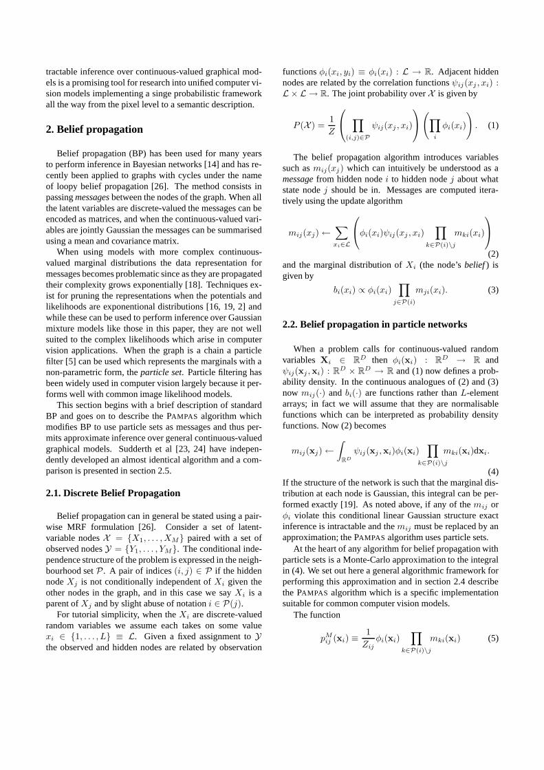
In the absence of image measurements the above modelis Gaussian and so the belief could be estimated by a vari-ety of methods. The cluttered image data used in figure 3causes the marginals to become highly non-Gaussian; thealgorithm converges on a globally plausible solution despitestrong local distractors. Here the φi used are simple robustgradient-affinity operators. The incorporation of informa-tion along the chain in both directions can be expected toimprove the performance of e.g. the Jetstream algorithm[21] which is a particle-based edge finder.

Figure 3. An edge linking model finds globalsolutions. The images show (in raster order)the belief estimates after 1, 5, and 10 itera-tions, and 7 samples from the joint graph af-ter 10 iterations. The belief stabilises on abimodal distribution with most of the weightof the distribution on the continuous edge ascan be seen on the bottom right image.

3.2. Illusory contour matching

We tested the algorithm on an illusory-contour find-ing problem shown in figure 4. The input image has C“pacman”-like corner points where the open mouth definestwo edge directions leading away from the corner separatedby an angle Cα. The task is to match up the edges withsmooth contours. We construct 2C chains each of fourlinks, and each is anchored at one end with a prior start-

ing at its designated corner pointing in one of the two edgedirections. At the untethered end of a chain from corner c isa “connector” edgel which is attached to (conditionally de-pendent on) the connectors at the ends of the 2C − 2 otherchains not starting from corner c. We use the same edgelmodel as in section 3.1 but now each node state-vector xi

is augmented with a discrete label υi denoting which of the2C − 2 partner chains it matches, and the potentials at theconnector are modified so that ψij(xj ,xi) = 0 when υi andυj do not match. This special form of potential allows usto form the message product in O(N 2C) operations ratherthan O(N2C−1) as a naive approach would dictate. Spacedoes not permit a full description of the algorithm here butit is very similar to the Mixed Markov Model approach [8].

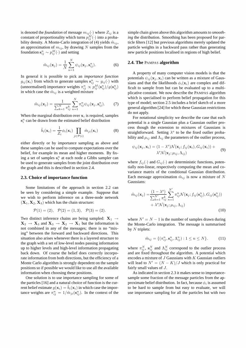
Figure 4 shows the model being applied to two scenarioswith C = 6 in both cases. First, Cα = 11π/36 whichleads to two overlapping triangles with slightly concaveedges when the chains are linked by the algorithm. Sec-ondly, Cα = 7π/9 which leads to a slightly convex regularhexagon. The same parameters are used for the models inboth cases, so the algorithm must adapt the edgel lengths tocope with the differing distances between target corners.

Figure 4. The PAMPAS algorithm performs illu-sory contour completion. Depending on theangle at which the chains leave the cornerpositions, the belief converges on either twooverlapping triangles or a single hexagon.

3.3. Finding a jointed object in clutter

Finally we constructed a graph representing a jointed ob-ject and applied the PAMPAS algorithm (combined with theGibbs sampler from [24]) to locating the object in a clut-tered scene. The model consists of 9 nodes; a central cir-cle with four jointed arms each made up of two rectangularlinks. The circle node x1 = (x0, y0, r0) encodes a positionand radius. Each arm node xi = (xi, yi, αi, wi, hi), 2 ≤i ≤ 9 encodes a position, angle, width and height andprefers one of the four compass directions (to break sym-metry). The arms pivot around their inner joints, so the po-

tential to go from an inner arm 2 ≤ i ≤ 5 to the outer armsj = i+ 4 is given by

xj = xi + hi cos(αi) +N (·; 0, σ2p)

yj = yi + hi sin(αi) +N (·; 0, σ2p)

αj = αi +N (·; 0, σ2α)

wj = wi +N (·; 0, σ2s ) hj = hi +N (·; 0, σ2

s)

and the ψ1i(xi,x1) from the circle outwards are similar.Going from the outer to the inner arm, the potential is notGaussian but we approximate it with the following:

xi = xj − hj cos(αi) +N (·; 0, hjσs| sin((i− 2)π/2)|σ2p)

yi = yj − hj sin(αi) +N (·; 0, hjσs| cos((i− 2)π/2)|σ2p)

αi = αj +N (·; 0, σ2α)

wi = wj +N (·; 0, σ2s ) hi = hj +N (·; 0, σ2

s ).

The ψi1(x1,xi) are straightforward:

x1 = xi +N (·; 0, σ2p) y1 = yi +N (·; 0, σ2

p)

r1 = 0.5(wi/δw + hi/δh) +N (·; 0, σ2s).

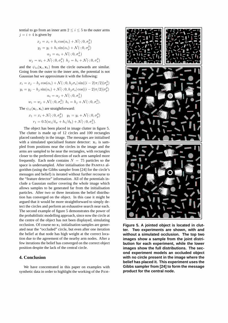
The object has been placed in image clutter in figure 5.The clutter is made up of 12 circles and 100 rectanglesplaced randomly in the image. The messages are initialisedwith a simulated specialised feature detector: x1 is sam-pled from positions near the circles in the image and thearms are sampled to be near the rectangles, with rectanglescloser to the preferred direction of each arm sampled morefrequently. Each node contains N = 75 particles so thespace is undersampled. After initialisation the PAMPAS al-gorithm (using the Gibbs sampler from [24] for the circle’smessages and belief) is iterated without further recourse tothe “feature detector” information. All of the potentials in-clude a Gaussian outlier covering the whole image whichallows samples to be generated far from the initialisationparticles. After two or three iterations the belief distribu-tion has converged on the object. In this case it might beargued that it would be more straightforward to simply de-tect the circles and perform an exhaustive search near each.The second example of figure 5 demonstrates the power ofthe probabilistic modelling approach, since now the circle atthe centre of the object has not been displayed, simulatingocclusion. Of course no x1 initialisation samples are gener-ated near the “occluded” circle, but even after one iterationthe belief at that node has high weight at the correct loca-tion due to the agreement of the nearby arm nodes. After afew iterations the belief has converged on the correct objectposition despite the lack of the central circle.

4. Conclusion

We have concentrated in this paper on examples withsynthetic data in order to highlight the working of the PAM-

Figure 5. A jointed object is located in clut-ter. Two experiments are shown, with andwithout a simulated occlusion. The top twoimages show a sample from the joint distri-bution for each experiment, while the lowerimages show the full distributions. The sec-ond experiment models an occluded objectwith no circle present in the image where thebelief has placed it. This experiment uses theGibbs sampler from [24] to form the messageproduct for the central node.

PAS algorithm. The applications we have chosen are highlysuggestive of real-world problems, however, and we hopethe promising results will stimulate further research intoapplying continuous-valued graphical models to a varietyof computer vision problems. Sections 3.1 and 3.2 suggesta variety of edge completion applications. Section 3.3 in-dicates that the PAMPAS algorithm may be effective in lo-cating articulated structures in images, in particular people.Person-finding algorithms exist already for locating andgrouping subparts [20] but they do not naturally fit into aprobabilistic framework. Recently several researchers havehad promising results finding jointed structures in imagesusing discretised graphical model representations [6, 10, 4].Both discretising and using the PAMPAS algorithm resultin approximations, and the tradeoffs between the two ap-proaches remain to be investigated.

One obvious advantage of using a graphical model rep-resentation is that it extends straightforwardly to tracking,simply by increasing the size of the graph and linking nodesin adjacent timesteps. Another area of great interest is link-ing the continuous-valued graph nodes to lower-level nodeswhich may be discrete-valued as in [13]. In fact, researchersin the biological vision domain have recently proposed ahierarchical probabilistic structure to model human visionwhich maps closely onto our algorithmic framework [17].

We are performing current research, to be published else-where, into the problem of sampling from products of Gaus-sian mixtures. The Gibbs sampler of [24] is very flexi-ble and straightforward to implement and performs well onsome important models, but for cluttered distributions ofthe type we have encountered K must be set prohibitivelylarge to get reliable samples. We have developed heuris-tic algorithms to address this clutter problem which per-form well on our test applications, but are only practicalfor D < 9. The design of an efficient, generally effectivesampler which scales to large D remains an open problem.

Acknowledgements

Helpful suggestions to improve this work were con-tributed by Michael Black, David Mumford, Mike Burrows,Martin Abadi, Mark Manasse and Ian Reid.

References

[1] J. August and S.W. Zucker. The curve indicator random field: curveorganization via edge correlation. In Perceptual Organization forArtificial Vision Systems. Kluwer Academic, 2000.

[2] C.M. Bishop, D. Spiegelhalter, and J. Winn. Vibes: A variationalinference engine for bayesian networks. In NIPS, 2002.

[3] X. Boyen and D. Koller. Tractable inference for complex stochasticprocesses. In Proceedings of the 14th Annual Conference on Uncer-tainty in Artificial Intelligence, 1998.

[4] J. Coughlan and S. Ferreira. Finding deformable shapes using loopybelief propagation. In Proc. 7th European Conf. Computer Vision,2002.

[5] A. Doucet, N. de Freitas, and N. Gordon, editors. Sequential MonteCarlo Methods in Practice. Springer-Verlag, 2001.

[6] P. Felzenszwalb and D. Huttenlocher. Efficient matching of pictorialstructures. In Proc. Conf. Computer Vision and Pattern Recognition,pages 66–73, 2000.

[7] W.T. Freeman, E.C. Pasztor, and O.T. Carmichael. Learning low-level vision. Intl. J. Computer Vision, 40(1):25–47, 2000.

[8] A. Fridman. Mixed markov models. In Proc. Second InternationalICSC Symposium on Neural Computation, 2000.

[9] S. Geman and D. Geman. Stochastic relaxation, Gibbs distributions,and the Bayesian restoration of images. IEEE Trans. on Pattern Anal-ysis and Machine Intelligence, 6(6):721–741, 1984.

[10] S. Ioffe and D. Forsyth. Human tracking with mixtures of trees. InProc. 8th Int. Conf. on Computer Vision, volume 1, pages 690–695,2001.

[11] M. Isard and A. Blake. Condensation — conditional density propa-gation for visual tracking. Int. J. Computer Vision, 28(1):5–28, 1998.

[12] M.A. Isard and A. Blake. A smoothing filter for Condensation. InProc. 5th European Conf. Computer Vision, volume 1, pages 767–781, 1998.

[13] N. Jojic, N. Petrovic, B. J. Frey, and T. S. Huang. Transformed hid-den markov models: Estimating mixture models of images and in-ferring spatial transformations in video sequences. In Proc. Conf.Computer Vision and Pattern Recognition, 2000.

[14] M.I. Jordan, T.J. Sejnowski, and T. Poggio, editors. Graphical Mod-els : Foundations of Neural Computation. MIT Press, 2001.

[15] M. Kass, A. Witkin, and D. Terzopoulos. Snakes: Active contourmodels. In Proc. 1st Int. Conf. on Computer Vision, pages 259–268,1987.

[16] D. Koller, U. Lerner, and D. Angelov. A general algorithm for ap-proximate inference and its application to hybrid bayes nets. In Pro-ceedings of the 15th Annual Conference on Uncertainty in ArtificialIntelligence, pages 324–333, 1999.

[17] T.S. Lee and D. Mumford. Hierarchical bayesian inference in thevisual cortex. Journal of the Optical Society of America A, 2002(submitted).

[18] U. Lerner. Hybrid Bayesian Networks for Reasoning about ComplexSystems. PhD thesis, Stanford University, October 2002.

[19] T.P. Minka. A family of algorithms for approximate Bayesian infer-ence. PhD thesis, MIT, January 2001.

[20] G. Mori and J. Malik. Estimating human body configurations us-ing shape context matching. In Proc. 7th European Conf. ComputerVision, pages 666–680, 2002.

[21] P. Perez, A. Blake, and M. Gangnet. Jetstream: Probabilistic contourextraction with particles. In Proc. 8th Int. Conf. on Computer Vision,volume II, pages 524–531, 2001.

[22] H. Sidenbladh, M.J. Black, and L. Sigal. Implicit probabilistic mod-els of human motion for synthesis and tracking. In Proc. 7th Euro-pean Conf. Computer Vision, volume 1, pages 784–800, 2002.

[23] E.B. Sudderth, A.T. Ihler, W.T. Freeman, and A.S. Willsky. Nonpara-metric belief propagation. Technical Report P-2551, MIT Laboratoryfor Information and Decision Systems, 2002.

[24] E.B. Sudderth, A.T. Ihler, W.T. Freeman, and A.S. Willsky. Non-parametric belief propagation. In CVPR, 2003.

[25] L.R. Williams and D.W. Jacobs. Stochastic completion fields: Aneural model of illusory contour shape and salience. Neural Compu-tation, 9(4):837–858, 1997.

[26] J.S. Yedidia, W.T. Freeman, and Y. Weiss. Understanding beliefpropagation and its generalizations. Technical Report TR2001-22,MERL, 2001.