THE UNIVERSITY OF KANSAS PALEONTOLOGICAL CONTRIBUTIONS October 31, 1966 Paper 10 QUANTITATIVE RE-EVALUATION OF ECOLOGY AND DISTRIBUTION OF RECENT FORAMINIFERA AND OSTRACODA OF TODOS SANTOS BAY, BAJA CALIFORNIA, MEXICO ROGER L. KAESLER Department of Geology, The University of Kansas ABSTRACT Environmental and faunal data on Foraminifera (WAL -roN, 1955) and Ostracoda (BENSON, 1959) from Todos Santos Bay, Baja California, were used to test applicability of quantitative methods of numerical taxonomy to biofacies analysis. Counts of specimens per species at each station were unreliable indicators of environmental similarity, particularly where total population was considered. Influencing the counts were such factors as mixing, differential productivity, and differential removal and destruction of subfossil forms. Presence-absence data were used. Biotopes were determined by clustering Q-matrices of simple matching coefficients; biofacies were determined by clustering R-matrices of Jaccard coefficients. The method used requires assumption of the existence of mappable biofacies and biotopes in the study area and adequate sampling, which at any time of year is considered representative of populations for the entire year. If total populations (live and dead forms together) are considered, the method requires that high positive correlation exists between distribution of the live and dead organisms. The method weights occurrence of each species equally for the purpose of delimiting biotopes (Q-technique) and occurrence of each species at each station equally for determining biofacies (R-technique). When these assumptions are satisfied, use of the numerical taxonomic method of biofacies analysis gives results closely similar to those based on qualitative interpretation. The quantitative method has the ad- vantages that results are objective and repeatable, computation is rapid, results may be expressed graphically, and choice of similarity level is clearly arbitrary and relative. INTRODUCTION SCOPE AND PURPOSE OF STUDY The purpose of this study is to investigate the applicability of the methods developed in numeri- cal taxonomy (SNEATH & SOKAL, 1962; SOKAL & SNEATH, 1963) to biofacies analysis. Todos Santos Bay, Baja California (Fig. 1), was chosen as the area of study because the ecology of the Recent Foraminifera (WALToN, 1955) and Ostracoda (BENSON, 1959) of that area has been thoroughly investigated. In order to succeed in this purpose it was necessary to examine the methods and con- clusions of both previous investigators in order to find relationships between their studies and strengths or weaknesses of their methods. Several terms used throughout this report re- quire definition and discussion. Biofacies analysis is the study of assemblages of organisms, their areal and chronologic distribu- tion, and environmental factors that affect them. The term biofacies has been defined and used in different ways (GLAESSNER, 1945, p. 183; IMBRIE, 1955,27, p. 450; TEICHERT, 1958, p. 2731-2734). For work on Recent organisms, both living and subfossil, the following definition is applicable: A biofacies is a group of organisms found together and presumably adapted to environmental condi- tions in their place of occurrence, such group dif- fering from contemporary assemblages found in

Welcome message from author
This document is posted to help you gain knowledge. Please leave a comment to let me know what you think about it! Share it to your friends and learn new things together.
Transcript

THE UNIVERSITY OF KANSAS
PALEONTOLOGICAL CONTRIBUTIONS
October 31, 1966 Paper 10
QUANTITATIVE RE-EVALUATION OF ECOLOGY ANDDISTRIBUTION OF RECENT FORAMINIFERA AND OSTRACODA
OF TODOS SANTOS BAY, BAJA CALIFORNIA, MEXICO
ROGER L. KAESLERDepartment of Geology, The University of Kansas
ABSTRACT
Environmental and faunal data on Foraminifera (WAL -roN, 1955) and Ostracoda (BENSON, 1959) fromTodos Santos Bay, Baja California, were used to test applicability of quantitative methods of numericaltaxonomy to biofacies analysis. Counts of specimens per species at each station were unreliable indicatorsof environmental similarity, particularly where total population was considered. Influencing the countswere such factors as mixing, differential productivity, and differential removal and destruction of subfossilforms. Presence-absence data were used. Biotopes were determined by clustering Q-matrices of simplematching coefficients; biofacies were determined by clustering R-matrices of Jaccard coefficients.
The method used requires assumption of the existence of mappable biofacies and biotopes in the studyarea and adequate sampling, which at any time of year is considered representative of populations for theentire year. If total populations (live and dead forms together) are considered, the method requires thathigh positive correlation exists between distribution of the live and dead organisms. The method weightsoccurrence of each species equally for the purpose of delimiting biotopes (Q-technique) and occurrence ofeach species at each station equally for determining biofacies (R-technique).
When these assumptions are satisfied, use of the numerical taxonomic method of biofacies analysis givesresults closely similar to those based on qualitative interpretation. The quantitative method has the ad-vantages that results are objective and repeatable, computation is rapid, results may be expressed graphically,and choice of similarity level is clearly arbitrary and relative.
INTRODUCTION
SCOPE AND PURPOSE OF STUDYThe purpose of this study is to investigate the
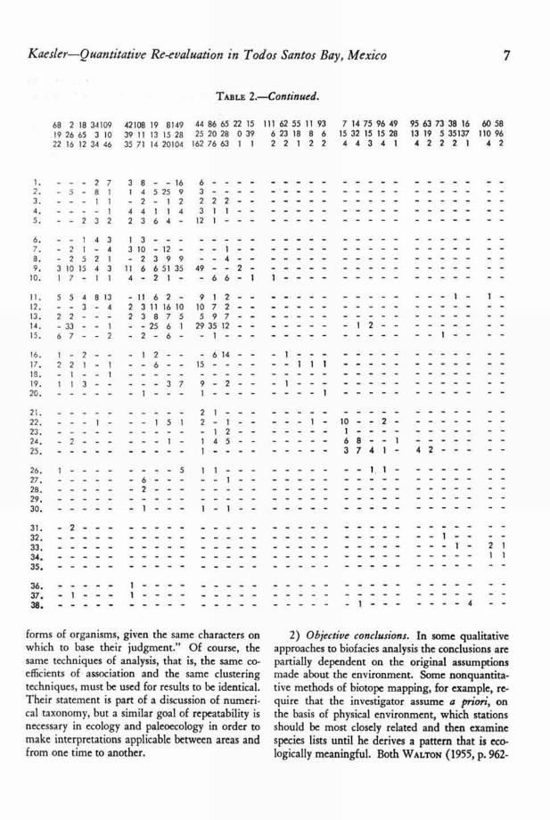
applicability of the methods developed in numeri-cal taxonomy (SNEATH & SOKAL, 1962; SOKAL &SNEATH, 1963) to biofacies analysis. Todos SantosBay, Baja California (Fig. 1), was chosen as thearea of study because the ecology of the RecentForaminifera (WALToN, 1955) and Ostracoda(BENSON, 1959) of that area has been thoroughlyinvestigated. In order to succeed in this purposeit was necessary to examine the methods and con-clusions of both previous investigators in order tofind relationships between their studies andstrengths or weaknesses of their methods.
Several terms used throughout this report re-quire definition and discussion.
Biofacies analysis is the study of assemblages oforganisms, their areal and chronologic distribu-tion, and environmental factors that affect them.The term biofacies has been defined and used indifferent ways (GLAESSNER, 1945, p. 183; IMBRIE,1955,27, p. 450; TEICHERT, 1958, p. 2731-2734).For work on Recent organisms, both living andsubfossil, the following definition is applicable: Abiofacies is a group of organisms found togetherand presumably adapted to environmental condi-tions in their place of occurrence, such group dif-fering from contemporary assemblages found in

2 The University of Kansas Paleontological Contributions—Paper 10
different environments. Transportation of sub- organisms are adapted may complicate biofaciesfossil material, or less commonly of living material, analysis. An assumption of paleoecology is thatto environments different from those to which the effects of transportation and mixing of faunas is
Kaesler—Quantitative Re-evaluation in Todos Santos Bay, Mexico 3
not great enough to obscure biofacies relationshipscompletely.
A biotic community (MAcGnsam, 1939) is an"assemblage of animals or plants [or both] livingin a common locality under similar conditions ofenvironment and with some apparent associationof activities and habits." The major difference be-tween a biofacies as defined above and a bioticcommunity is the element of association of activi-ties and habits. One may discuss biofacies withoutreference to the effects organisms may have oneach other, whereas inherent in the communityconcept is the idea of structure and interactionamong the organisms. In addition, the communityconcept involves organisms of many kinds, in con-trast to biofacies which may relate to a single kindof organism (e.g., ostracodal biofacies, foramini-feral biofacies).
The term biotope has also been used in differ-ent contexts. Discussing the biotic communityHEDGPETH (in HEDGPETH et al., 1957, p. 40) con-sidered biotope or environment as the "particularplace" occupied by organisms of a community.THORSON (1957, p. 473) equated biotope with sub-stratum in his discussion of sublittoral or shallow-shelf bottom communities. In paleoecologic workon Permian reefs NEWELL (1957, p. 433) consid-ered biotopes to be ecological zones, but not in achronologic sense. HESSE, ALLEE, & SCHMIDT
(1937, p. 135) defined biotope as the "primarytopographic unit" of ecology comprising "an areaof which the principal habitat conditions and theliving forms . . . adapted to them are uniform."In this study biotope is recognized as an area ofrelatively uniform environmental conditions evi-denced by a particular fauna found in the area andpresumably adapted to environmental conditionsexisting there. Thus it is possible to speak of theostracodal biotopes or foraminiferal biotopes ofTodos Santos Bay.
Numerical taxonomy (SHEATH & SOKAL, 1962,p. 2) is "the numerical evaluation of the affinityor similarity between taxonomic units and theordering of these units into taxa on the basis oftheir affinities." In ecologic or paleoecologicstudies the "taxonomic units" are ecologic units(stations), and the "taxa" are biotopes. It is be-lieved that these methods will help give the samerepeatability and objectivity to paleoecology whichthey provide for taxonomy.
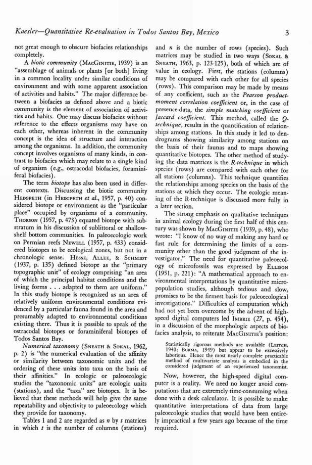
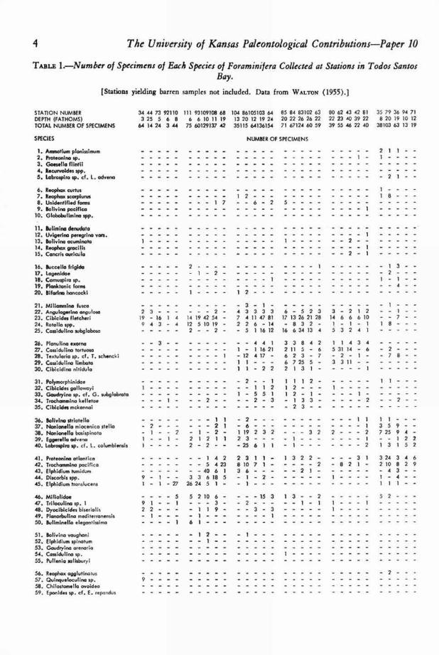
Tables 1 and 2 are regarded as n by t matricesin which t is the number of columns (stations)
and n is the number of rows (species). Suchmatrices may be studied in two ways (SoKAL &SHEATH, 1963, p. 123-125), both of which are ofvalue in ecology. First, the stations (columns)may be compared with each other for all species(rows). This comparison may be made by meansof any coefficient, such as the Pearson product-moment correlation coefficient or, in the case ofpresence-data, the simple matching coefficient orlaccard coefficient. This method, called the Q-technique, results in the quantification of relation-ships among stations. In this study it led to den-drograms showing similarity among stations onthe basis of their faunas and to maps showingquantitative biotopes. The other method of study-ing the data matrices is the R-technique in whichspecies (rows) are compared with each other forall stations (columns). This technique quantifiesthe relationships among species on the basis of thestations at which they occur. The ecologic mean-ing of the R-technique is discussed more fully ina later section.
The strong emphasis on qualitative techniquesin animal ecology during the first half of this cen-tury was shown by MACGINME (1939, p. 48), whowrote: "I know of no way of making any hard orfast rule for determining the limits of a com-munity other than the good judgment of the in-vestigator." The need for quantitative paleoecol-ogy of microfossils was expressed by ELLIsox(1951, p. 221): "A mathematical approach to en-vironmental interpretations by quantitative micro-population studies, although tedious and slow,promises to be the firmest basis for paleoecologicalinvestigations." Difficulties of computation whichhad not yet been overcome by the advent of high-speed digital computers led IMBRIE (27, p. 454),in a discussion of the morphologic aspects of bio-facies analysis, to reiterate MACGINITIE ' S position:
Statistically rigorous methods are available (LErrcx,1940; BURMA, 1949) but appear to be excessivelylaborious. Hence the most nearly complete practicablemethod of multivariate analysis is embodied in theconsidered judgment of an experienced taxonomist.
Now, however, the high-speed digital com-puter is a reality. We need no longer avoid com-putations that are extremely time-consuming whendone with a desk calculator. It is possible to makequantitative interpretations of data from largepaleoecologic studies that would have been entire-ly impractical a few years ago because of the timerequired.
4 The University of Kansas Paleontological Contributions-Paper 10
TABLE 1.-Number of Specimens of Each Species of Foraminifera Collected at Stations in Todos SantosBay.
[Stations yielding barren samples not included. Data from WALTON (1955).]
STATION NUMBERDEPTH (FATHOMS)TOTAL NUMBER OF SPECIMENS
SPECIES
34 44 73 92110325 568
64 14 24 3 44
111 93109108 68 6 6 10 11 19
75 60129137 42
104 86105103 64 85 84 83102 63
13 20 12 19 24 20 22 26 26 22
35115 64136154 71 67124 60 59
NUMBER OF SPECIMENS
80 62 43 42 8122 23 40 39 2239 55 46 22 40
35 79 36 94 718 20 19 10 12
38103 63 13 19
1. Ammotium plonissirnum 2 1 1 - -
2. Proteonino sp. 13. Geesello flintii4. Recurvoides spp.5. Labrospiro sp. cf. L. odveno 2 1 - -
6. Reophax curtus7. Reophax scorpion's 1 2 8. Unidentified forms ----- - - - 17 --6-2 5 9. Bolivina pacific°
10. Globobu liming spp.
11. Sulimina denudata12. Uvigerino peregrina vars.13. &olivine ocuminota 1 -----
14. Reophan gracilis15. Cancris ouricula 2-1
16. Batten° frigido 2 I I 3 - -
17. Logeniclae 1 2 2
18. Cornuspira sp. 1
19. Planktonic forms 4
20. Etiforina honcocki 1 1 2
21. Miliaminina fusca -3-1- 1
22. Angulogerino onguloso 2 3 ------ 2- 4 3 3 3 3 6 - 5 2 3 3 - 2 1 2 --1-
23. Cibicides fletcheri 19 - 16 1 4 14 19 42 54 - 7 4 11 47 81 17 13 26 21 28 14 6 6 6 10 - - 7 -
24. Rotalia spp. 9 4 3 - 4 12 5 10 19 - 2 2 6 - 14 -832- 1 - 1 1 1 8 - -
25. Cassidulina subglobosa 2 2 5 1 16 12 16 6 34 13 4 5 3 2 4 1
26. Planulina exorne --3 -- ----- 441 3 3 8 4 2 1 1 4 3 4
27. Cossidulina tortuoso 1 - 1 16 21 2 11 5 - 6 5 31 14 6 - 2 -
28. Textularia sp. cf. T. schencki ----- - - - - 1 - 12417- 6 2 3 - 7 1 -78
29. Cassidulina limboto 1 1 - - - 6 7 25 5 - 3311 - - -
30. Cibicidino nitidula 1 1 2 2 2131 1
31. Polymorphinidoe 2 1 I I 1 2 1 1 - -
32. Cibicides gallowayi 1 ----------- 1 1 2 1 2 - - - 1
33. Goudryina sp. cf. G. subglobrata 1 5 5 1 1 2 1 1
34. Trochammino kelletoe 1 - 2 - 2 - 3 1 3 3 - 2 2
35. Cibicides mckannai 2 3
36. Bolivina striotello -- - 1 1 2 1 1 1 1 -
37. Nonionello rniocenica steno 2 ------ 2 1 6 1 3 5 9 - -
38. Nonionella besispinato 1 2 - 1 - 2 1 19 2 3 2 - - - 3 2 2 - 2 7 25 9 4 -
39. Eggerella odvena 1 - - 1 - 2 1 2 1 1 2 3 - 1 - - I - - 1 2 2
40. Labrospira sp. cf. L. columbiensis 1 - 2 - 2 - - 25 6 1 1 - 1 ------ 2 1 3 1 5 1
41. Proteonina atlantic° -- 1 4 2 2 3 1 1 - 1 3 2 2 - - 3 1 3 24 3 4 6
42. Trochornmino pacific° 5 4 23 8 10 7 1 ----- 2 - 8 2 1 2 10 8 2 9
43. Elphidium tornidum ---- - - 40 6 1 3 6 ----- 2 1 4 3 -
44. Discorbis spp. 9 - 1 - - 3 3 6 18 5 -1-2- 1 -
45. Elphidium tronslucens 1 - 1 - 27 26 24 5 1 1 1 1 1 - -
46. Miliolidoe - - - - 5 5210 6 1 3 2 5 2
47. Triloculina sp. I 9 1 - - 1 3 1 1
48. Dyocibicides biseriolis 2 2 - 1 1 9 3 3 1 - - - - -----
49. Plonorbulino mediterronensis - 1
50. Buliminella elegantissima - - - - 1 6 1
51. &olivine, voughoni 12 1
52. Elphidium spinoturn 1 53. Goudryina cyclonic54. Cassidulina sp.55. Pullenia salisburyi
56. Reophox agglutinotus 2
57. Quinqueloculino sp. 9
58. Chilostomella ovoideo
59. Eponides sp. cf. E. repandus

Kaesler-Quantitative Re-evaluation in Todos Santos Bay, Mexico
TABLE 1.-Continued.
5
75 76 91 90 54 51 74 89 88 77 78 95 96 97 87 56 70 55 69 50 67 49 48 65 66 57 38 39 47 61 59 60 45 58 3715 16 11 13 11 12 12 15 16 16 17 13 15 15 12 24 17 18 19 20 24 28 30 28 27 31 35 68108 92 110110141 96 2517 21 24 37 5 1 18 32 57 8 22 39 44 23 63 13 27 63 33 65 67 44 91230105 117155103 80 40 88 43102144 93
NUMBER OF SPECIMENS
1. ----- - - 216- -28411 2 - - 1 - 2 1 14 2 4 Il -I 12. --12- 2 1 2 - - 611 - 1 13. 2 6 1 6 5 6 3! - 1 24. 1 1 2 - 3 2 8 4 1 13 3 1 - --12 -5. 1 1 1 1 13 4 - 1 - - 13 ------- 6
6. 2 15 1 6 6 5 17 74 6 12 -------- 4 7. 2 - 2 - - 3 1 1 4 6 14 533 8 10 1 ------- 4 8.9.10.
10 11 13 - - 112
- 7 1 - -4 4 1 941 7 33 26 8
- 1 - 43 832 5 -8 10 38 25
12.1 2 1 - 15 - 27 10 13 20 1
2 2 - 11 1 32313. 1 5 3 5 15 11 4 1 1614. - -l- 1 4 2 3 4 1 -II- -15. 1 - 1 1 1 ----- 1
16. 2 2 4 1 - 1 517.18.
--- 21 12
- - 2 11 - 2 819.
20.1
48 6
1
21.222. 1 - 4 - 2 1 ----- 5 23. 8 3 11 2 4 -24. 2 1 1 4 6 - - 20 2 ----125.
-- -171 2444 - 2 1 5 6 6
26. 2 1 127.
128. 1 1 - 1 -29. 130.
31.32.
- - - 1 3
33.34. 2 235.
36. 2-1 ---77 2106 - - - - 1 1137. - 1 4 -------- 4 - 3 4 4 36 32 24 77 34 8 5 6 - 726 1338. 2 1 3 2 5 1--10 8 4 139.40.
I 13113 8 1 11
-- - 10 11 1
-662-9 12 7 4 25
-1-3-2 3 5 1 - 2 - 51 6 6 1 5 -2-31
41. 8 11 10 12 -217182 9 9 3 2 20 -514124 4 1 2 - 3 --- 1 5 2 - 2 -42. 5 1 78 4 113 3123 I 29-3 2 11 25820 8 9 2 8 7 4 -43. 1 ---------- 1144 , 1--4 15 1 - -45.
46. 4 -
47. 248.49.50. 3
51. 2152.53. 254. 5 ---I55. 1
56. -----
57.58. 659. 1
6 The University of Kansas Paleontological Contributions-Paper 10
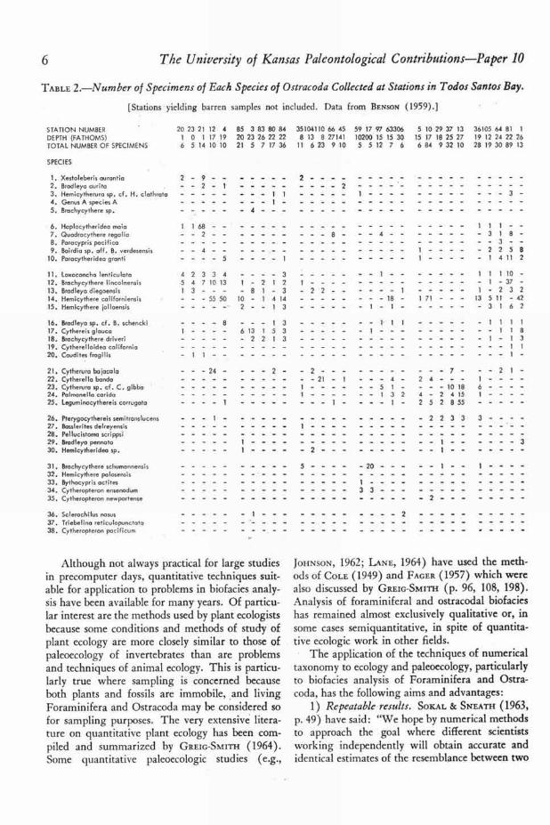
TABLE 2.-Number of Specimens of Each Species of Ostracoda Collected at Stations in Todos Santos Bay.
[Stations yielding barren samples not included. Data from BENSON (1959).]
STATION NUMBER 20 23 21 12 4 85 3 83 80 84 35104110 66 45 59 17 97 63306 5 10 29 37 13 36105 64 81 1
DEPTH (FATHOMS) 1 0 1 17 19 20 23 26 22 22 8 13 8 27141 10200 15 15 30 15 17 18 25 27 19 12 24 22 26
TOTAL NUMBER OF SPECIMENS 6 5 14 10 10 21 5 7 17 36 11 6 23 9 10 5 5 12 7 6 684 9 32 10 28 19 30 89 13
SPECIES
1. Xestoleberis aurantia 2 - 9 - 22. Bradley° aurita - 2 - 1 - - - - - 23. Hemicytherura sp. cf. H. clathrate 1 3
4. Genus A species A5. Brachycythere sp. 4
6. Haplocytheridea maia 1 1 68 I 1 1 -
7. Quadracythere regalia - 2 - 8 4 --- - 318-
8. Paracypris pacifica -- 3 --9. Bairdia sp. off. B. verdesensis 4 -225 8
10. Paracytheridea granti - 1 I 4 11 2
11. Loxoconcha lenticulata 4 2 3 3 4 - 3 1 I 1 10 -
12. Brachycythere lincolnensis 5 4 7 10 13 1 - 212 1 - - 1 - 37 -
13. Bradley° diegoensis 1 3 - - - - 8 1 - 3 2 2 1 - 2 3 2
14. Hemicythere californiensis - - - 55 50 10 - 1 4 14 -- 18 1 71 - 13 5 11 - 42
15. Hernicythere jollaensis 2 - 13 1-1 - 3162
16. Bradley° sp. cf. B. schencki -- B -13 1 1 1 I 1 1
17. Cythereis glouce 6 13 153 1 118
18. Brachycythere driver i 2 213 13
19. Cytherelloldea colifornia 120. Caudites frogilis 1f 1
21. Cytherura bajocala - - 24 - - 2 - 2 - 2 1 -
22. Cytherella banda 21 - 4- 2 4 - - - 123. Cytherura sp. cf. C. gibba 5 1 - - 10 18 624. Polmonello corido 132 4 2 4 15 125. Leguminocythereis corrugate - 1 1 2 5 2 8 55
26. Pterygocythereis sernitrenslucens 223 3 327. Basslerites delreyensis28. Pellucistoma scrippsi29. Bradley° pennata 330. Hemicytheridea sp. 2
31. Brachycythere schurnannensIs I - -
32. Hemicythere palosens1s33. Bythocypris actites 134. Cytheropteron ensenadum 3335. Cytheropteron newportense 2
36. Sclerochilus nasus37. Triebelina reticulopunctata38. Cytheropteron pacificum
1 2
Although not always practical for large studiesin precomputer days, quantitative techniques suit-able for application to problems in biofacies analy-sis have been available for many years. Of particu-lar interest are the methods used by plant ecologistsbecause some conditions and methods of study ofplant ecology are more closely similar to those ofpaleoecology of invertebrates than are problemsand techniques of animal ecology. This is particu-larly true where sampling is concerned becauseboth plants and fossils are immobile, and livingForaminifera and Ostracoda may be considered sofor sampling purposes. The very extensive litera-ture on quantitative plant ecology has been com-piled and summarized by GREIG-SMITH (1964).Some quantitative paleoecologic studies (e.g.,
JOHNSON, 1962; LANE, 1964) have used the meth-ods of COLE (1949) and FACER (1957) which werealso discussed by GREIG-SMITH (p. 96, 108, 198).Analysis of foraminiferal and ostracodal biofacieshas remained almost exclusively qualitative or, insome cases semiquantitative, in spite of quantita-tive ecologic work in other fields.
The application of the techniques of numericaltaxonomy to ecology and paleoecology, particularlyto biofacies analysis of Foraminifera and Ostra-coda, has the following aims and advantages:
1) Repeatable results. SOKAL & SNEATH (1963,p. 49) have said: "We hope by numerical methodsto approach the goal where different scientistsworking independently will obtain accurate andidentical estimates of the resemblance between two
Kaesler-Quantitative Re-evaluation in Todos Santos Bay, Mexico 7
TABLE 2.-Continued.
1.2.3.4.5.
68 2 18 34109
19 26 65 3 1022 16 12 34 46
---27-5-81
- 1 1
- - 1--232
42108 19 814939 11 13 15 2835 71 14 20104
3 8 - - 161 4 5 25 9-2-124 4 1 1 42364
44 86 65 22 1525 20 28 0 39
162 76 63 I 1
6 3 222 311
12 1
Ill 62 556 23 18
2 2 1
1182
9362
7154
14 75 96 4932 15 15 284 3 4 1
95 63 73 38 1613 19 5 351374 2 2 2 1
60 58110 964 2
6. - - 1 4 3 1 3
6
7. - 2 I - 4 3 10 - 12 - - - 18. - 2 5 2 1 -2399 4 9. 3 10 15 4 3 11 6 6 51 35 49 - - 2
10. 1 7 - I I 4 - 2 1 - -66-1 1
11. 5 5 4 8 13 - 11 6 2 - 912 ---------- - - - 1 - 1 -
12. 3 - 4 2 3 11 16 10 10 7 213. 2 2 - - 2 3 8 7 5 597 14. - 33 - - 1 - - 25 6 1 29 35 12 12
15. 6 7 - 2 -2-6-2-6- - I 1
16. 1 - 2 - - 1 2 - - 6 1417. 2 2 1 - 1 - 6 - 15IS.19. 1 1 3 - - --37 9 - 2 - - - 120. 1 1
21. 2 122. - - 1 5 1 2 - 1 - - 1 - 10 - - 2 - -----
23. 1 2 1 24. 2 - 1 4 5 - - ----- 6 8 - - 125. ----- 3 7 4 1 - 4 2 - -
26. 11- 1 127. 6 -- 128. 229.30. 1 1
31. - 232. 1 - -
33. 1 2134. 11
35.
36.37.38. 1 4 -
forms of organisms, given the same characters onwhich to base their judgment." Of course, thesame techniques of analysis, that is, the same co-efficients of association and the same clusteringtechniques, must be used for results to be identical.Their statement is part of a discussion of numeri-cal taxonomy, but a similar goal of repeatability isnecessary in ecology and paleoecology in order tomake interpretations applicable between areas andfrom one time to another.
2) Objective conclusions. In some qualitativeapproaches to biofacies analysis the conclusions arepartially dependent on the original assumptionsmade about the environment. Some nonquantita-tive methods of biotope mapping, for example, re-quire that the investigator assume a priori, onthe basis of physical environment, which stationsshould be most closely related and then examinespecies lists until he derives a pattern that is eco-logically meaningful. Both WALTON (1955, p. 962-
— 31°52' vv,„
116° 40'
BAHIA de TODOS SANTOS
" • BAJA CALIFORNIA
1 • '• •
116° 46";::
NAUTICAL MILESIMMIN11111=n0 I 2 3
116° 46'
8
The University of Kansas Paleontological Contributions—Paper 10
964) and BENSON (1959, p. 34, 35) arranged their though BENSON modified this order in his study tostations in order of increasing depth of water, al- fit the ostracodal biofacies, which were not as
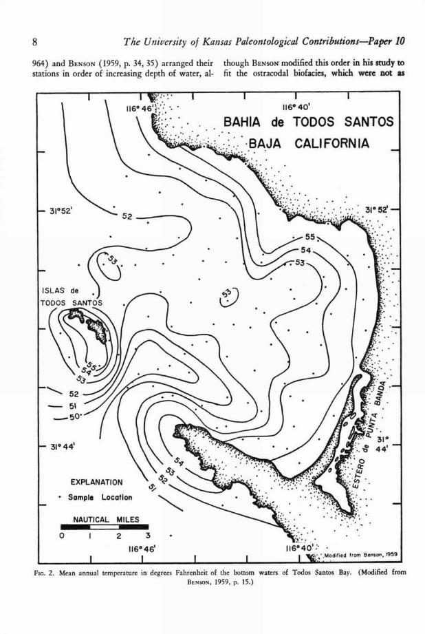
F c. 2. Mean annual temperature in degrees Fahrenheit of the bottom waters of Todos Santos Bay. (Modified fromBENSON, 1959, P. 15.)

Kacsler—Quantitative Re-evaluation in Todos Santos Bay, Mexico 9
strongly controlled by depth as were WALTON ' S
foraminiferal biofacies. Similarly BENSON & KAES-
LER in their study of the Ostrocoda of the Esterode Tastioto (1963, p. 10-12) initially arranged sta-tions a priori on the basis of their increasing dis-tance from (and, hence, supposed dissimilarity to)open Gulf of California stations. In a large orcomplex study area in which biotope boundariesare not well defined, the final interpretation coulddepend to a considerable extent on such initial as-sumptions. If results of Recent ecologic studies areto be applied to study of ancient environments, amethod must be found which enables investigatorsto make interpretive statements about ancient phy-sical environments on the basis of biotope maps,rather than the converse. Numerical taxonomictechniques in ecology eliminate the bias describedabove and make Recent ecologic interpretationsmore applicable to studies of ancient environments.
3) Rapid computations. The computation ofsimilarity coefficients and clustering of these co-efficients into dendrograms was done very rapidlywith a digital computer. Once a computer pro-gram for the computations was available, the com-puter time for even a relatively large study (suchas 65 stations, 59 species) was almost negligible.
4) Graphic representation. Recognition of eco-logically meaningful patterns in large matrices ofnumbers is an extremely difficult or even impos-sible task for the human mind. Representation ofclusters of similarity by dendrograms (SNEATH &
SOKAL, 1962, p. 10-11) obviates this difficulty andreplaces it was an easily interpreted, graphic por-trayal of similarities among ecologic units clus-tered. The use of a dendrogram, which is a 2-dimensional representation of multidimensional re-lationships, results in some loss of information(SoKAL & SNEATH, 1963, p. 198-203). The magni-tude of the loss of information and an estimate ofthe closeness of fit of the dendrogram to the matrixmay be obtained by the method used by ROHLF
(1963). Furthermore, dendrograms express simi-larities as hierarchies, even though ecologic rela-tionships may not be so structured. I believe thatdistortion of information in this way is not seriouswhen compared with the shortcomings of alterna-tive methods.
5) Free choice of similarity level. Up to thispoint I have stressed the advantages of a mathe-matically rigorous method of biofacies analysis.Any method of clustering, whether quantitative orqualitative, has a principal weakness in the neces-
sarily subjective choice of the limiting level ofassociation. Qualitative methods may use "na-tural breaks" or "best fits" to the physical environ-ment. Statistical methods, such as those of FAGER
(1957), JoHNsoN (1962), or any of several dis-cussed by GREIG-SMITH (1964), use a statisticallevel of significance which is chosen arbitrarily.Other quantitative techniques (FAGER & McGow-AN, 1963; LANE, 1964) choose arbitrary levels. Thenumerical taxonomic dendrograms have the ad-vantage that their "arbitrariness and relativity isobvious" (SNEATH & SOKAL, 1962, p. 12) and un-obscured, as in the purely qualitative or statisticalmethods.
PREVIOUS STUDIESECOLOGY OF FORAMINIFERA
WALTON (1955, p. 958) gave a thorough re-view of studies of the ecology of Foraminifera offthe west coast of the United States made before1955. Many workers (NATLAND, 1933; BUTCHER,
1951; CROUCH, 1952; and BANDY, 1953) consideredtemperature to be much more important thandepth in controlling distribution of benthonicforms. Other studies of the ecology of Foramini-fera include work by PHLEGER (39-44), PHLEGER
& WALTON (45), PARKER, PHLEGER & PIERSON
(38), BANDY (3), BANDY et al. (4), and WALTON
(64).
ECOLOGY OF OSTRACODAAn exhaustive list of ecological studies of Os-
tracoda has been given by BENSON (1959, p. 5-6).Two important papers not included there arestudies of Ostracoda and Foraminifera of the Firthof Clyde (ROBERTSON, 1875) and the paleoecologyof Pleistocene beds of Scotland (CaossaEy & Roa-ERTSON, 1875). Since BENSON completed his work,the ecology and distribution of Recent Ostracodain North America have been studied by PUR! &
HULINGS (47), BENDA & PUR! (5), BENSON & COLE-
MAN (7), and BENSON & KAESLER (8). A sym-posium (PUR!, et al., 46) held in Naples in 1963dealt with the subject "Ostracods as Ecological andPaleoecological Indicators."
FIELD AND LABORATORYTECHNIQUES
STUDY OF FORAMINIFERAWALTON (1955, p. 958-961) gave a complete
discussion of field and laboratory techniques used
1 v».• • r116° 46";:: '• ' 1l6°40'
BAHIA de TODOS SANTOS
. ..BAJA CALIFORNIA
ISLAS de
TODOS SANTOS
44'
o
EXPLANATION
• Sample Location
Phytal Zone
NAUTICAL MILES111111=11111E=111111=0 T 2 3
116° 46'
10
The University of Kansas Paleontological Contributions—Paper 10
by him in studying the Foraminifera of Todos one-mile grid on February 5, 1952, and additionalSantos Bay. He took samples on an approximate samples along a traverse from shallow to deep
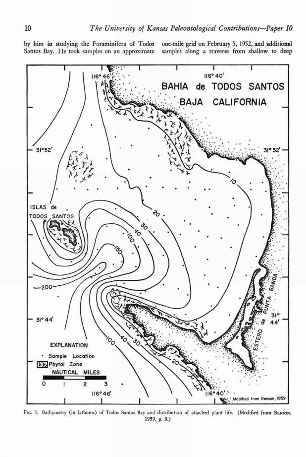
Fic. 3. Bathymetry (in fathoms) of Todos Santos Bay and distribution of attached plant life. (Modified from BENSON,
1959, p. 9.)
Kaesler—Quantitative Re-evaluation in Todos Santos Bay, Mexico 11
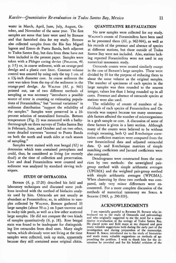
water in March, April, June, July, August, Oc-tober, and November of the same year. The firstsamples are some that later were used by BENSONand that furnished data for my study. BENSONalso collected samples from the Rio San Miguellagoon and Estero de Punta Banda, both adjacentto Todos Santos Bay, but data from these have notbeen included in the present paper. Samples weretaken with a Phleger coring device ( PHLECER, 40,p. 3-5) or, in coarse sediment, with an orange-peeldredge and a plastic core liner. Constant volumecontrol was assured by using only the top 1 cm. ofa 1%-inch diameter core. In coarse sediment thecore was taken from the top of the sediment in theorange-peel dredge. As WALTON (63, p. 960)pointed out, use of two different methods ofsampling as was necessary "introduces a possiblesource of error in counting or estimating popula-tions of Foraminifera," but "normal variations" insediment distribution "support the reliability ofthe samples." Samples were preserved in a 10-percent solution of neutralized formalin. Bottomtemperature (Fig. 2) was measured with a bathy-thermograph on three surveys of Todos Santos Bayin February, June, and October and on two other,more detailed traverses "normal to Punta Bandaon both the north and south sides at each seasonof sampling."
Samples were stained with rose bengal (62) todetermine which tests contained protoplasm andcould, thus, be considered as living (or recentlydead) at the time of collection and preservation.Live and dead Foraminifera were counted andsediment was analyzed by standard sieving tech-niques.
STUDY OF OSTRACODA
BENSON (6, p. 17-20) described his field andlaboratory techniques and discussed some prob-lems involved with the method of biofacies analy-sis used by him. Ostracoda are not usually asabundant as Foraminifera; so, in addition to sam-ples collected by WALTON, BENSON gathered 33large samples (about 50 cc.) on 3-part traverse andin rocky tide pools, as well as a few other scatteredlarge samples. He did not compare the two kindsof samples quantitatively (6, p. 18). Rose bengalstain was found to be inadequate for distinguish-ing live ostracodes from dead ones. Many singlevalves, which obviously were not living at the timesamples were collected, took up stain, apparentlybecause they still contained some original chitin.
QUANTITATIVE RE-EVALUATIONNo new samples were collected for my study.
WALTON'S counts of Foraminifera have been usedas he presented them (63, p. 962-964), as well ashis records of the presence and absence of speciesat different stations, but those outside of TodosSantos Bay were not included. Also, stations lack-ing reported Foraminifera were not used in mynumerical taxonomic study.
Ostracode counts were treated similarly exceptin the case of BENSON'S large samples. These weredivided by 10 for the purpose of reducing them toabout the same volume as the original samples.The number of specimens of each species in thelarge samples was then rounded to the nearestinteger, values less than 1 being rounded up in allcases. Presence and absence of ostracode species atstations were also used.
The reliability of counts of numbers of in-dividuals of each species of Foraminifera and Os-tracoda was suspect because too many unmeasur-able factors affected the number of microorganismsin a grab sample or core. A discussion of some ofthese factors is given in a later section. Althoughmany of the counts were believed to be withoutecologic meaning, both Q- and R-technique corre-lation coefficient matrices were computed from theraw foraminiferal data and adjusted ostracodaldata. Q- and R-technique matrices of simplematching coefficients and Jaccard coefficients werealso computed.
Dendrograms were constructed from the mat-rices by two methods: the unweighted pair-group method with simple arithmetic averages(UPGMA) and the weighted pair-group methodwith simple arithmetic averages (WPGMA).When clustering by these two methods was com-pared, only very minor differences were en-countered. For a more complete discussion of themethods of numerical taxonomy see SOKAL &SNEATH (1963, p. 290-319).
ACKNOWLEDGMENTSI am especially grateful to RICHARD H. BENSON who in-
troduced me to the study of Ostracoda and paleoecologyand who originally suggested to me the need for a quan-titative re-evaluation of the ecology of Todos Santos Bay.He placed notes and field maps at my disposal and gavemany valuable suggestions both during the early part of theinvestigation and during preparation of the manuscript.ROBERT R. SOKAL introduced me to the study of biometricsand made many valuable suggestions on methods of ap-proaching the problem. I wish to thank him for the in-spiration he provided and for his helpful criticism of the
12
The University of Kansas Paleontological Contributions—Paper 10
typescript. I am indebted to A. J. ROWELL for many help-ful suggestions concerning methods applicable to the studyand review of the contents of this report. I also thankF. JAMES ROHLF, who aided by computing some of the firstdendrograms used in the study, and NORMAN HERTFORDand PAUL A. TomAs, both of whom helped with problemsof programming and computation. Many of the ideas inthis study were developed during discussions with ROSALIEF. MADDOCKS.
Work on the Todos Santos Bay problem was begun inthe summer of 1963 during my tenure as a National Sci-
ence Foundation Summer Fellow at the University of Kan-sas. The study was supported further by a National ScienceFoundation Fellowship at the University of Kansas for theacademic year 1964-1965. A grant from the University ofKansas Computation Center provided support for computertime, and many staff members of the center helped whenneeded. A grant from the University of Kansas supple-mented the National Science Foundation Fellowship bysupporting research and manuscript preparation.
Work was done using facilities of the University ofKansas Museum of Invertebrate Paleontology.
DESCRIPTION OF STUDY AREA, ENVIRONMENTAL FACTORS,
AND SAMPLING
DESCRIPTION OFTODOS SANTOS BAY
Todos Santos Bay is located about 40 nauticalmiles southeast of the United States-Mexico bor-der on the west coast of Baja California (Fig. 1).Its northern edge is formed by an indentation inthe coast and its southern boundary by the penin-sula Punta Banda which juts from the coastline atan angle of about N. 45° W. Two islands, the Islasde Todos Santos, lie four or five miles northwestof the seaward extremity of Punta Banda. The bayis nearly square and measures about eight miles ona side.
A complete description of the study area hasbeen given by WALTON (63, p. 953-958) and BEN-
SON (6, p. 6-12), including observations on the baymargins, surrounding geology, and geomorphol-ogy. Following is a summary of BENSON ' S descrip-tion of the coast of Todos Santos Bay.
The northern margin of the bay consists ofnarrow beaches, terraces, and sea cliffs with somerocky tide pools. The eastern coast has a widesand beach, the southern half of which makes upa sand spit separating the Estero de Punta Bandafrom Todos Santos Bay. The southern coast re-sembles the northern but is even more rocky, withonly isolated crescent beaches.
Mean annual temperature of bottom watersand water depths of Todos Santos Bay are shownin Figures 2 and 3. The temperature data wererecorded at each station by WALTON (63, p. 960)on February 4, June 4, and October 9, 1952, usinga bathythermograph. He also took more detailedtemperature data as mentioned above. Mean an-nual bottom temperatures range from about 55°F.in shallow water to about 50°F. in the deep chan-nel. In shallow water near the shore the annualtemperature range is about 10°F., but in the deep-
est part of the channel it ranges only about 2 °F.annually.
Figure 3 also shows distribution of attachedplant life, principally Macrocystis and Laminaria(6, p. 9). Depth throughout most of the arearanges from 10 to 20 fathoms. A deep channelbetween Punta Banda and the south island con-nects Todos Santos Bay with the open ocean, asdoes the broad northwest margin of the bay.
The effect of depth on distribution of Foramin-ifera (NATLAND, 1933; BUTCHER, 1951; CROUCH,
1952; BANDY, 1953; WALTON, 1955) and Ostracoda(REmANE, 1933; ELOFSON, 1941; BENSON, 1959;BENSON & COLEMAN, 1963; Ascou, 1964) is com-plex. Commonly depth is found to be correlatedclosely with many other environmental factorssuch as temperature, nearness to shore, degree oflight penetration, wave base, and in some casessediment size and salinity. Thus temperature,usually strongly correlated with depth, has beenconsidered more important than depth itself as afactor controlling distribution of Foraminifera.BENSON & COLEMAN (1963, p. 11) considered depthas a useful aggregate factor expressing the effectsof all the above environmental factors on the ostra-code fauna. Relationship of depth to other en-vironmental factors and faunistic characteristics ofTodos Santos Bay will be discussed in a later sec-tion. Table 3 shows the depth in fathoms at eachof WALTON ' S original stations.
Of much less importance to benthonic Ostra-coda and Foraminifera is surface temperaturewhich, like the nearshore bottom temperature,
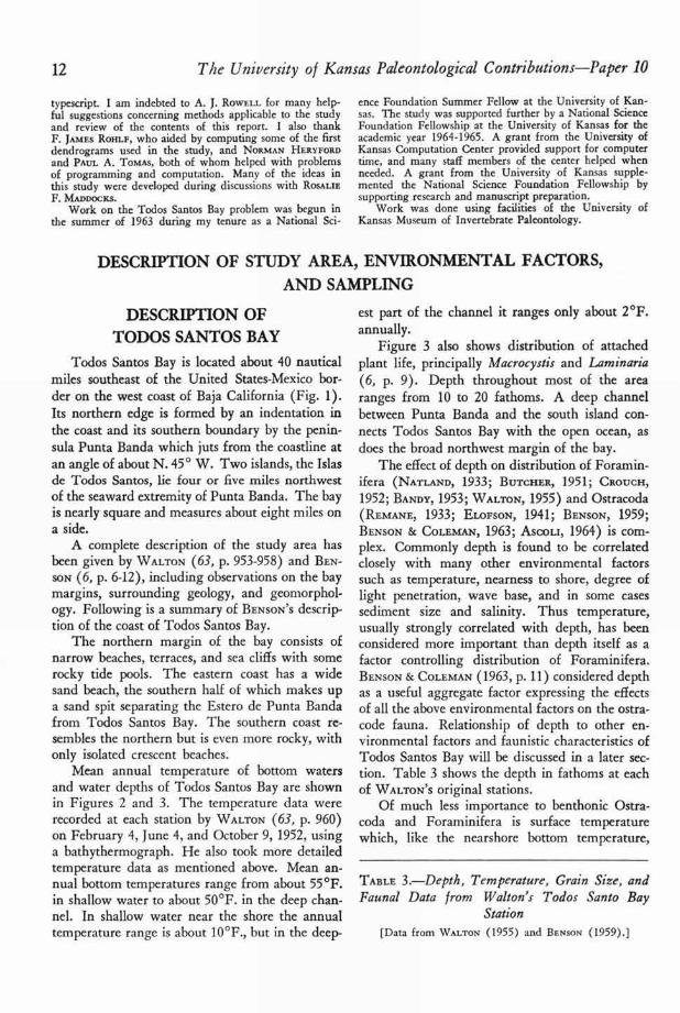
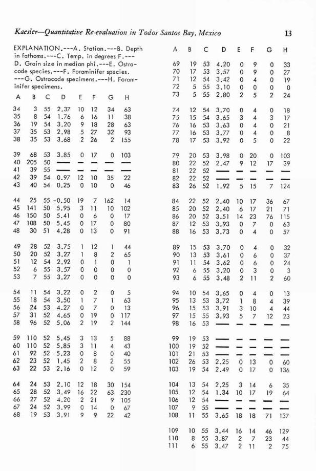
TABLE 3.—Depth, Temperature, Grain Size, andFaunal Data from Walton's Todos Santo Bay
Station[Data from WALTON (1955) and BENSON (1959).]
Kaesler-Quantitative Re-evaluation in Todos Santos Bay, Mexico 13
EXPLANATION.---A. Station.---B. Depthin fathoms.---C. Temp. in degrees F.---D. Grain size in median phi.---E. Ostra-code species.---F. Foraminifer species.
---G. Ostracode specimens.---H. Foram-inifer specimens.
A BCD EF GH
34 3 55 2.37 10 12 34 6335 8 54 1.76 6 16 11 3836 19 54 3.20 9 18 28 6337 35 53 2.98 5 27 32 9338 35 53 3.68 2 26 2 155
39 68 53 3.85 0 17 0 10340 205 50 ----41 39 55
0.97 2242 39 54 12 10 3543 40 54 0.25 0 10 0 46
44 25 55 -0.50 19 7 162 1445 141 50 5.95 3 11 10 10246 150 50 5.41 0 6 0 1747 108 50 5.45 0 17 0 8048 30 51 4.28 0 13 0 91
49 28 52 3.75 1 12 1 4450 20 52 3.27 1 8 2 6551 12 54 2.92 0 1 0 152 6 55 3.57 0 0 0 053 7 55 3.27 0 0 0 0
54 11 54 3.22 0 2 0 555 18 54 3.50 1 7 1 6356 24 53 4.27 0 7 0 1357 31 52 4.65 0 19 0 11758 96 52 5.06 2 19 2 144
59 110 52 5.45 3 13 5 8860 110 52 5.85 3 11 4 4361 92 52 5.23 08 0 4062 23 52 1.45 2 8 2 5563 22 53 2.16 0 12 0 59
64 24 53 2.10 12 18 30 15465 28 52 3.49 16 22 63 23066 27 52 4.20 2 21 9 10567 24 52 3.99 0 14 0 6768 19 53 3.91 9 9 22 42
AB C DEF GH
69 19 53 4.20 0 9 0 3370 17 53 3.57 0 9 0 2771 12 54 3.42 0 4 0 1972 5 55 3.10 0 0 0 073 5 55 2.80 2 5 2 24
74 12 54 3.70 0 4 0 1875 15 54 3.65 3 4 3 1776 16 53 3.63 0 4 0 2177 16 53 3.77 0 4 0 878 17 53 3.92 0 5 0 22
79 20 53 3.98 0 20 0 10380 22 52 2.47 9 12 17 3981 22 52 ----82 22 52 ----
1.9283 26 52 5 15 7 124
84 22 52 2.40 10 17 36 6785 20 52 2.40 6 17 21 7186 20 52 3.51 14 23 76 11587 12 53 3.93 0 7 0 6388 16 53 3.73 0 4 0 57
89 15 53 3.70 0 4 0 3290 13 53 3.61 0 6 0 3791 11 54 3.62 0 6 0 2492 6 55 3.20 03 0 393 6 55 3.48 2 11 2 60
94 10 54 3.65 0 4 0 1395 13 53 3.72 1 8 4 3996 15 53 3.91 3 10 4 4497 15 55 3.93 5 7 12 2398 16 53 - -
99 19 53100 19 52101 21 53
2.25102 26 53 0 13 0 60103 19 54 2.49 0 17 0 136
104 13 54 2.25 3 14 6 35105 12 54 1.34 10 17 19 64106 12 54107 9 55 -- --
108 11 55 3.65 18 18 71 137
109 10 55 3.44 16 14 46 129110 8 55 3.87 2 7 23 44111 6 55 3.47 2 11 2 75
14
The University of Kansas Paleontological Contributions—Paper 10
varies seasonally about 10°F. The minimum re-corded temperature is 57.0°F. in March; the maxi-mum known is 67.8°F. in August. WALTON (63,p. 961) reported that surface temperatures duringFebruary, March, and April are quite uniform inTodos Santos Bay.
Average surface temperature in June and July(63, p. 966) is 61.8°F., but protected parts of thebay may have temperatures as high as 65°F. A 9°or 10°F. temperature difference between the warmnorthern and cool southern sides of Punta Bandais common in June, and as great a difference as21°F. has been recorded. This difference may beascribed to upwelling along the south side ofPunta Banda (63, p. 966) which occurs in Juneand July. In August the 10°F. temperature differ-ence remains, but water both within the bay andon the south side of Punta Banda is considerablywarmer. By October and November surface tem-perature within the bay decreases to about 61 °F.and upwelling diminishes so that little temperaturedifferential exists (63, p. 966).
Water in the Estero de Punta Banda is verywarm in the spring and summer months. Its in-fluence on the temperature of the water in TodosSantos Bay near the mouth of the estuary is in-creased by the 3.8 foot tidal range (63, p. 966).
Salinity in the open ocean off Punta Bandaranges from 33.40%0 in the winter to 33.70%0 inthe spring and summer. WALTON (63, p. 966) con-sidered this to be a fairly good estimate of salinityin most of the bay, but salinity probably has awider range of variation near the mouth of theEstero de Punta Banda. If the salinity is as nearlyconstant as indicated, it seems doubtful that itwould have any appreciable effect on faunal distri-bution.
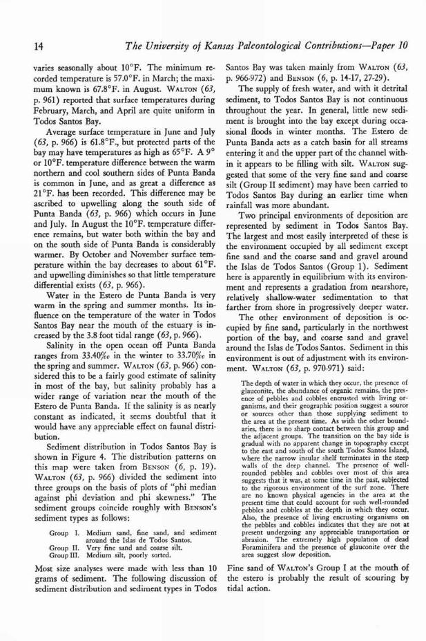
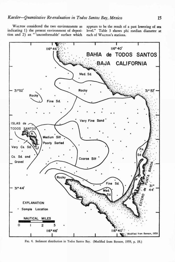
Sediment distribution in Todos Santos Bay isshown in Figure 4. The distribution patterns onthis map were taken from BENSON (6, p. 19).WALTON (63, p. 966) divided the sediment intothree groups on the basis of plots of "phi medianagainst phi deviation and phi skewness." Thesediment groups coincide roughly with BENSON ' Ssediment types as follows:
Group I. Medium sand, fine sand, and sedimentaround the Islas de Todos Santos.
Group II. Very fine sand and coarse silt.Group III. Medium silt, poorly sorted.
Santos Bay was taken mainly from WALTON (63,p. 966-972) and BENSON (6, p. 14-17, 27-29).
The supply of fresh water, and with it detritalsediment, to Todos Santos Bay is not continuousthroughout the year. In general, little new sedi-ment is brought into the bay except during occa-sional floods in winter months. The Estero dePunta Banda acts as a catch basin for all streamsentering it and the upper part of the channel with-in it appears to be filling with silt. WALTON sug-gested that some of the very fine sand and coarsesilt (Group II sediment) may have been carried toTodos Santos Bay during an earlier time whenrainfall was more abundant.
Two principal environments of deposition arerepresented by sediment in Todos Santos Bay.The largest and most easily interpreted of these isthe environment occupied by all sediment exceptfine sand and the coarse sand and gravel aroundthe Islas de Todos Santos (Group 1). Sedimenthere is apparently in equilibrium with its environ-ment and represents a gradation from nearshore,relatively shallow-water sedimentation to thatfarther from shore in progressively deeper water.
The other environment of deposition is oc-cupied by fine sand, particularly in the northwestportion of the bay, and coarse sand and gravelaround the Islas de Todos Santos. Sediment in thisenvironment is out of adjustment with its environ-ment. WALTON (63, p. 970-971) said:
The depth of water in which they occur, the presence ofglauconite, the abundance of organic remains, the pres-ence of pebbles and cobbles encrusted with living or-ganisms, and their geographic position suggest a sourceor sources other than those supplying sediment tothe area at the present time. As with the other bound-aries, there is no sharp contact between this group andthe adjacent groups. The transition on the bay side isgradual with no apparent change in topography exceptto the east and south of the south Todos Santos Island,where the narrow insular shelf terminates in the steepwalls of the deep channel. The presence of well-rounded pebbles and cobbles over most of this areasuggests that it was, at some time in the past, subjectedto the rigorous environment of the surf zone. Thereare no known physical agencies in the area at thepresent time that could account for such well-roundedpebbles and cobbles at the depth in which they occur.Also, the presence of living encrusting organisms onthe pebbles and cobbles indicates that they are not atpresent undergoing any appreciable transportation orabrasion. The extremely high population of deadForaminifera and the presence of glauconite over thearea suggest slow deposition.
Most size analyses were made with less than 10 Fine sand of WALTON ' S Group I at the mouth ofgrams of sediment. The following discussion of the estero is probably the result of scouring bysediment distribution and sediment types in Todos tidal action.
Maw .111•••
. -
1 .
116° 46'
1
116°40' :• •
V.,: : Modified from Benson, 19591116°46'
1
1160401
•. BAHIA de TODOS SANTOS. ...BAJA CALIFORNIA
Fine Sd.
•
31°44' —
EXPLANATION
• Sample Location
NAUTICAL MILES11=1===1M11111110 I 2 3 • • • •
31° 52' —
Kaesler—Quantitative Re-evaluation in Todos Santos Bay, Mexico 15
WALTON considered the two environments as appears to be the result of a past lowering of seaindicating 1) the present environment of deposi- level." Table 3 shows phi median diameter attion and 2) an " `unconformable' surface which each of WALTON ' S stations.
Fin. 4. Sediment distribution in Todos Santos Bay. (Modified from BENSON, 1959, p. 19.)

16 The University of Kansas Paleontological Contributions—Paper 10
TABLE 4.—Correlation Coefficients Computed Between Variables in Table 3.[Underlined values are significantly different from zero at 95-percent level.]
(A) Depth
(B) Temperature
(C) Grain size
(D) Ostracociespecies
(E) Foraminiferspecies
(F) Ostracodespecimens
(G) Foraminiferspecimens
(A)
-0.6648
(B)
-0.0966
0.1164
-0.2324
(C)
-0.0278
0.4649
(D)
0.4083
(E)
0.2483
0.8529
(F) (G)
0.2270
0.0941
-0.1036
0.0926
-0.0852
0.1144
0.1156
-0.2394
-0.1203
0.4175
0.8762
0.4027
QUANTITATIVE RELATIONSHIPSAMONG ENVIRONMENTAL
FACTORSA thorough discussion of the ecology of Fora-
minifera and Ostracoda was given by WALTox(1955) and BENSON (1959). For details the readeris referred to their studies. Here I consider onlysome of the gross quantitative aspects of the ecol-ogy.
The lower half matrix in Table 4 gives correla-tion coefficients among depth, temperature, sedi-ment size, and four faunal characteristics of the 78stations in Todos Santos Bay occupied by WALTON.
Values of r significantly different from zero at the95 percent level are underlined. For discussion ofthese coefficients the reader is referred to anystandard statistical text.
Calculation of correlation coefficients requiresthe assumption that a linear relationship exists be-tween variables within the population, which isvalid when sampling is from a bivariate normaldistribution (STEEL & TORRIE, 1960, p. 183). Atest of the data of Table 3 for normal distributionusing probability paper gave the following results:
1) Depth. Slightly skewed right, but probably notsignificantly so.
2) Temperature. Slightly leptokurtic, but probablyno significantly so.
3) Sediment size. Slightly leptokurtic.4) Number of ostracode species. Not normally
distributed, but very much like a Poisson distributionbut with considerable contagion. Neither square rootnor log transformations improve normality of thesedata appreciably.
5) Number of foraminifer species. Very good fitto normal distribution.
6) Number of ostracode specimens. Strongly platy-ku rtic.
7) Number of foraminifer specimens. Slightlyplatykurtic, but probably not significantly differentfrom a normal distribution.
The assumption of normally distributed data, then,is at least roughly met in all cases except numberof ostracode species and specimens.
Table 4 shows a negative correlation betweendepth and temperature. This is what one wouldexpect a priori since temperature generally de-creases with increased depth. If we ignore thecorrelation coefficients involving the ostracodedata, the only other statistically significant co-efficients are between foraminiferal categories andboth temperature and sediment size. The negativecorrelation between temperature and both fora-minifer species and foraminifer specimens is onlybarely significant, but it shows at least a slight in-crease in number of species and individuals withdecrease in temperature.
Of more significance is the correlation betweengrain size and the two bodies of data on Foramin-ifera. An increase in median phi size of the sedi-ment correlates with increase in both number offoraminifer species and number of foraminiferspecimens. Because phi size is the negative loga-rithm to the base 2 of the grain size in millimeters,the larger the positive phi value, the smaller thesediment size. Thus, decrease in grain size is ac-companied by an increase in both number of fora-
Kaesler—Quantitative Re-evaluation in Todos Santos Bay, Mexico 17
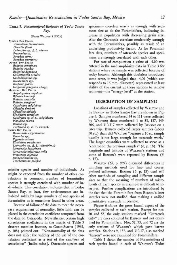
TABLE 5. Foraminiferal Bio facies of Todos SantosBay.
[From WAL.rox (1955)]MIDDLE BAY FACIES
Ammotium planissimumGoesella fiintiiLabrospira sp. cf. L. advenaProteonina sp.Reophax curtusReophax scorpiurus
OUTER BAY FACIES
Bolivina acuminataBolivina pacificaBulimina denudataChilostomella ovoideaGlobobulimina spp.Recurvoides spp.Reophax gracilisUvigerina peregrina subspp.
MARGINAL BAY FACIES
Angulogerina angulosaBifarina hancoek;Bolivina striatellaBolivina vaughaniCassidulina subglobosaCibicides fietcheriCibicidina nitidulaElphidium turnidumGaudryina sp. cf. G. subglabrataPlanulina exornaRotalia spp.Textularia sp. cf. T. schencki
INNER BAY FACIES
Buliminella elegantissimaDiscorbis spp.EggertIla advenaElphidium translucensLabrospira sp. cf. L. columbiensisNonionella basispinataNonionella miocenica stellaProteonina atlantic°Quinqueloculina sp.Trocham mina pacifica
minifer species and number of individuals. Asmight be expected from the number of other cor-relations in common, number of foraminiferspecies is strongly correlated with number of in-dividuals. This correlation indicates that in TodosSantos Bay, at least, few environments are in-habited solely by large numbers of one species offoraminifer as is sometimes found in other areas.
Because of failure of the data to meet the neces-sary requirement of normality, little faith can beplaced in the correlation coefficient computed fromthe data on Ostracoda. Nevertheless, certain highcorrelations coefficients in the matrix of Table 5deserve mention because, as GREIG-SMITH (1964,p. 108) pointed out: "Non-normality of the datadoes not affect the validity of the use of the cor-relation coefficient as a test of the existence ofassociation" [italics mine]. Ostracode species and
specimens correlate nearly as strongly with sedi-ment size as do the Foraminifera, indicating in-crease in population with decreasing grain size.Also the Ostracoda correlate moderately stronglywith the Foraminifera, possibly as result of anunderlying productivity factor. As for Foramini-fera data, numbers of ostracode species and speci-mens are strongly correlated with each other.
For ease of computation a value of –4.00 wasentered in the median-phi-size data in Table 3 forstations where no sample was collected because ofrocky bottom. Although this doubtless introducedsome error, it was judged that –4.00 (which cor-responds to 16 mm. diameter) represented at leastability of the current at those stations to removesediment—the "energy level" at the station.
DESCRIPTION OF SAMPLING
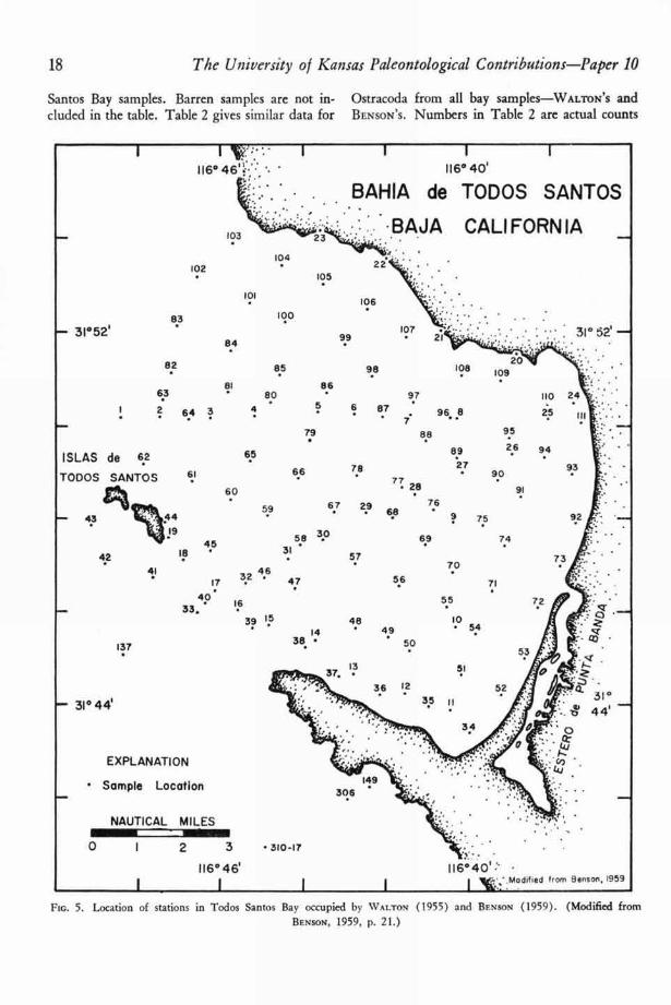
Locations of samples collected by WALTON andby BENSON in Todos Santos Bay are shown in Fig-ure 5. Samples numbered 34 to 111 were collectedby WALTON; those numbered 1 to 33, 137, 149,306, and 310-317 were collected by BENSON On alater trip. BENSON collected larger samples (about50 cc.) than did WALTON "because a 10-cc. sampleusually is not large enough for ostracode work."The larger quantities were collected to serve as a"control on the previous samples" (6, p. 18). Thelongitude and latitude of WALTON ' S stations andsome of BENSON ' S were reported by BENSON (6,p. 17).
WALTON (63, p. 959) discussed differences insampling methods used for fine- and coarse-grained sediments. BENSON (6, p. 18) used stillother methods of sampling and different samplesizes so that the meaning of numbers of micro-fossils of each species in a sample is difficult to in-terpret. Further complications are introduced bythe fact that the Foraminifera from BENSON'S latersamples were not studied, thus making a unifiedquantitative approach impossible.
Figure 6 shows the gross faunal aspect of thesamples collected at each station. Except for nos.50 and 55, the only stations marked "Ostracodaonly" are ones collected by BENSON and not exam-ined for Foraminifera. Nos. 52, 53. and 72 are theonly stations of WALTON ' S which gave barrensamples. Stations 9, 137, and 310-17, also marked"barren" were not examined for Foraminifera.
Table 1 shows the number of Foraminifera ofeach species found in each of WALTON ' S Todos
81 86
580
4 • 6 87
79
65
7866
6077
• 28
766.8
75
6.9 74
116 ° 40' :" •v.,' : Modified from Benson, 1959
1•
6.3
2 64 3
^
17
40 •
33. •
116° "
103
116° 40'
. BAHIA de TODOS SANTOS
•BAJA CALIFORNIA104
102105
106
oo
— 31 0 52' 10799• 21
84
85 98 108
ISLAS de 6.2
TODOS SANTOS
43
45
42
137
— 310441
EXPLANATION
• Sample Location149
306 •
8.3
82109
91
73
71
•••••••I
67 29
57
32 4
.6 47 56
70
16 55
10• 54
95
26
90
NAUTICAL MILESnM:=1111111111111110 I 2 3 • 310-17
116° 46 1
61
18
97
. 96 87
88
89
27
59
39
5831 •
18
The University of Kansas Paleontological Contributions—Paper 10
Santos Bay samples. Barren samples are not in- Ostracoda from all bay samples—WALTON'S andeluded in the table. Table 2 gives similar data for BENSON'S. Numbers in Table 2 are actual counts
Flo. 5. Location of stations in Todos Santos Bay occupied by WALTON (1955) and BENSON (1959). (Modified fromBENSON, 1959, P. 21.)

• •
•
• •
• •
116° 40'
. BAHIA de TODOS SANTOS
•BAJA CALIFORNIA••
•
e e e
••
• • ••
•••
o •
e Ostracoda only e31° 44' • Foraminifera only •,.;,... • c)
• Ostracoda and Foraminifer°,• Barren
NAUTICAL M ILES11111••1=MIIMIIII0 I 2 3 • - • '
EXPLANATION
1160 46 f• • '
Kaesler—Quantitative Re-evaluation in Todos Santos Bay, Mexico 19
and are not adjusted for unequal sample sizes, cording to the order of stations and species in theStations and species are arranged in the tables ac- dendrograms in Figures 10, 14, 20, and 23.
FIG. 6. Gross faunal aspect of the samples collected at each station in Todos Santos Bay. (Data from WALTON, 1955,and BENSON, 1959.)

20
The University of Kansas Paleontological Contributions—Paper 10
BIOFACIES ANALYSIS
INTRODUCTION
Determination of foraminiferal and ostracodalbiofacies and subdivision of Todos Santos Bay intobiotopes constituted a major portion of bothWALTON ' S and BENSON ' S studies. WALTON (63,p. 960) based his biofacies analysis on living orrecently dead forms that contained enough proto-plasm to be stained by rose bengal. BENSON (6,p. 20) worked with both stained forms and emptycarapaces and thus established biofacies on thebasis of total population, not living population.
Both WALTON and BENSON made a qualitativeor semiquantitative approach to biofacies analysisof Todos Santos Bay, but their results have some-what different meaning because their methods offormulating biofacies were slightly different. WAL-TON (63, p. 979) restricted species of Foraminiferato only one biofacies, for he excluded from all bio-facies species that occurred abundantly in morethan one environment or not abundantly in anyenvironment. As one might expect, few species fi tinto a biofacies perfectly. For example, Reophaxgracilis (KIAER), which lives at depths of 10 to400 fathoms in Todos Santos Bay and adjacentparts of the open Pacific Ocean (63, p. 1013), wasincluded in the outer bay facies because it is mostcommon between 50 and 100 fathoms. SimilarlyAngulogerina angulosa (WILLiAmsoN) was in-cluded in the marginal bay facies because, althoughit lives at depths of 3 to 360 fathoms in the studyarea, it is most abundant between 20 and 100fathoms. Throughout his study WALTON weighteddepth very strongly, but it is important to note thatdistribution of only species of the outer bay faciesseems to be controlled dominantly by depth orenvironmental factors highly correlated withdepth. Table 5 gives a list of foraminiferal bio-facies as determined by WALTON (63, p. 979-981),who wrote the following in explaining his bio-facies (p. 979):
The living representatives of the benthonic fora-miniferal species in Todos Santos Bay generally fi tinto four areal assemblages. The boundaries of theseassemblages are generalized but the species associatedwith each assemblage occur most abundantly withinthe areas outlined in [his text] Figure 14.
BENSON ' S (6, p. 28, 29) ostracodal biofacies areshown in Table 6. He did not restrict ostracodespecies to a single biofacies, for both Hemicytherecaliforniensis LERoy and Cytherura bajacala BEN-
SON belong to more than one biofacies, and H.californiensis LERoy was considered a "significantfacies indicator" (6, p. 34). Still other species arefound in more than one biofacies if BENSON ' S en-tire study is considered rather than the stations
TABLE 6. Ostracoda Bio facies of Todos Santos Bay.[From BENSON (1959) 1
ROCKY TIDE POOLSBrachycythere lincolnensisCaudites fragilisHaplocytheridea maiaLoxoconcha lenticulataXestoleberis aura ntia
BIOFACIES IBairdia sp. all. B. verdesensisBrachycythere driveniBrachycythere lincolnensisBradleya auritaBradleya diegoensisBradleya pennataCythereis glattcaCytheurara bajacalaHemicythere californiens sHemicythere jollaensisHemicytherura sp. cf. H. clath rataParacytheridea grantiQuadracythere regalia
BIOFACIESBrachycythere sp.Cytherella bandaCytherura bajacalaCytherura sp. cf. C. gibbaHemicythere californiensisLeguminocythereis corrugataPalmanella caridaParacypris pacificaPterygocythereis sein itranslucens
BIOFACIES IVBythocypris actitesCytheropteron newportenseCytheropteron pacificum
from Todos Santos Bay alone. Furthermore, BEN-SON (personal communication) grouped stationstogether on the basis of their similarity of fauna inorder to estimate similarity of response to environ-ment.
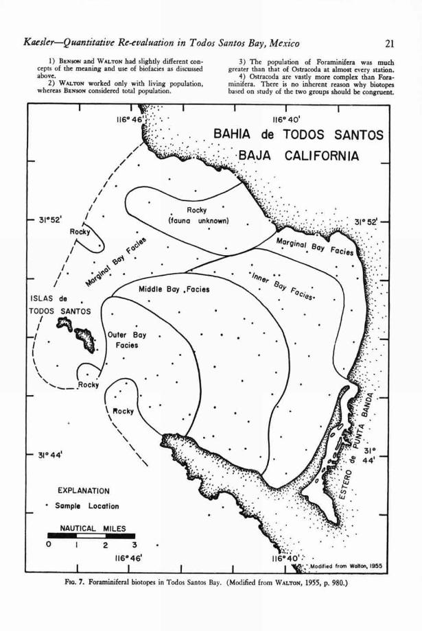
A map of the foraminiferal biotopes in TodosSantos Bay (63, p. 980) is shown in Figure 7 andBENSON'S ostracodal biotopes are indicated in Fig-ure 8. The lack of congruence of these two mapsis perhaps not as great as first appears. The dis-tributions of Walton's marginal bay facies and partof BENSON ' S biofacies I agree quite closely. Simi-larly part of WALTON'S outer-bay facies is identicalin distribution with BENSON ' S biofacies IV.
Nevertheless, important differences do exist be-tween the two interpretations, some of which maybe explained as follows:
""--"
•
31°44' —
— 3044'
1 Rocky
••
116° 40'
BAHIA de TODOS SANTOS
• • BAJA CALIFORNIA
Avr
• •V''`‘ *•§I.• \t'' .
NO 4
ISLAS de
TODOS SANTOS
/' Igtit4
•_Rocky
Outer Bay .Facies
•
wn•••1
NAUTICAL MILES1111C71111=1110 I 2 3
116° 46'
Kaesler—Quantitative Re-evaluation in Todos Santos Bay, Mexico
21
1) BENSON and WALTON had slightly different con-cepts of the meaning and use of biofacies as discussedabove.
2) WAL-roN worked only with living population,whereas BENSON considered total population.
3) The population of Foraminifera was muchgreater than that of Ostracoda at almost every station.
4) Ostracoda are vastly more complex than Fora-minifera. There is no inherent reason why biotopesbased on study of the two groups should be congruent.
Fia. 7. Foraminiferal biotopes in Todos Santos Bay. (Modified from WALT0N, 1955, p. 980.)

116° 40'
BAHIA de TODOS SANTOS
" CALI FORN IA _
NAUTICAL MILES1111111111111=1111111=0t 2 3
116°46'
22
The University of Kansas Paleontological Contributions—Paper 10
They are members of different phyla; their needs aredifferent; their methods of reproduction are different;their modes of life are different. Why, then, shouldnot their responses to their environments be different?
WALTON'S marginal-bay biotope on the north-west margin of the bay corresponds with the dis-tribution of sediment group I (63, p. 969), an area
Flo. 8. Ostracodal biotopes in Todos Santos Bay. (Modified from BENSON, 1959, p. 31.)
Kaesler—Quantitative Re-evaluation in Todos Santos Bay, Mexico 23
in which very little sediment is now being de-posited. The ostracodal biotopes (Fig. 8) are veryclosely related to sediment distribution (Fig. 4).The only major deviation from this pattern is thearea of biotope III (barren), which transects sedi-ment-type boundaries.
QUANTITATIVE RE-EVALUATION
ASSUMPTIONS
As stated above, the major purpose of thisstudy is to determine applicability of the numeri-cal taxonomic methods Of SOKA L & SNEATH
(1963) to biofacies analysis. Three assumptions ofall hiofacies analysis of the type done by WALTON(1955) and BENSON (1959) are: 1) Biofacies andbiotopes exist in the study area. 2) A sample ade-quately represents the population of organisms ata station. 3) Biotopes are mappable.
The first assumption merely requires that wenot impose a system on nature where none exists.In an area such as Todos Santos Bay, where en-vironmental factors vary geographically and aremappable, there is little doubt that real biofaciesand biotopes exist, although a certain amount oftransition from one biofacies or biotope to anotheris to be expected. GREIG-SMITH (1964, p. 132), indiscussing the reality of plant communities,pointed out that the idea of the existence of sep-arate plant communities need not be rejected evenif one does not accept the organismal concept of acommunity (CLEMENTS, 1916). GREIG-SMITH fur-ther said (1964, p. 132):
If species had ranges of tolerances in relation to en-vironmental differences that tended to coincide, sothat the total number of species in a region could bearranged in a considerably smaller number of groups,the members of each having approximately the samelimits of tolerance, then distinctive communities, withmore or less well-defined boundaries, would be ex-pected, each corresponding to, and composed of, oneof the groups of species of similar tolerance.
GREIG-SMITH (1964, p. 132, 133) also pointed outthat "extensive examination of the limits of tol-erance of a geographical group of species in rela-tion to all environmental factors" has not beenmade and is very likely an impossibility and that"an objective assessment of the reality of plantcommunities" should be made in an area occupiedby more than one community. The preceding dis-cussion applies equally well to hiofacies as to plantcommunities.
If the conditions of the second assumption arenot met, that is, if two samples taken from thesame locality at the same time have a statisticallysignificant difference in number of specimens orpresence-absence patterns, then we can hardly ex-pect to draw conclusions about differences amongstations. If sampling is adequate, differences inmethod of sampling should make no difference ex-cept in actual number of specimens found. Ade-quacy of sampling has not been tested in any studyof biofacies analysis of microfossils, but M. A.Buzas, U.S. National Museum (personal com-munication), has designed a sampler which willcollect multiple samples from one station andwhich he hopes to use to obtain data for such atest.
If the conditions of the third assumption arenot met, that is, if biotopes are not largely con-tinuous geographically, the results of clusteringstations into biotopes may appear to be entirelymeaningless. If biotopes are real (see assumption1), they are probably mappable, although sampledensity may be insufficient to bring out their arealextent. The organisms that make up a biofaciesare affected by environmental factors such asdepth, temperature, and sediment size, all ofwhich can be mapped. The aggregate effect ofthese factors should produce a faunal group witha distribution geographically continuous enoughto be mapped.
Another assumption must be made when astudy includes samples taken at only a few timesof the year: 4) An adequate sample (in the senseof assumption 2) taken at any time of the yearrepresents the population for the entire year. Thisassumption is probably rarely justified if the studyconsiders only living organisms which have a sea-sonal variation. But in a study like BENSON ' S(1959) in which total population is considered,dead individuals, which may have accumulatedfor several years, usually far outweigh living ones.In this kind of study conditions of the assumptionare probably met unless some of the species aredestroyed or removed much more rapidly thanothers.
Another assumption that applies only to studiesof total population should be stated. 5) A highpositive correlation exists between the distributionof live and dead organisms. This assumption isnecessary if the biofacies analysis is to be at allapplicable to paleoecology. If dissimilarity between

Er'
24 The University of Kansas Paleontological Contributions—Paper 10
CORRELATION COEFFICIENT
-1.0 -0.8 -0.6 -0.4 -0.2 0.0 0.2 0.4 06 0.8 1.0
STATIONS
3410973
108103636480818485
1028342
1051049293Ill11062433586979495
r-=
IIn••nn11
8789767890
8896
367954516850917569
74717055
77 56 48 67 49 37
6638
57 39 65 44
61 58 59
47Fr— 45 60
1 I I I I I I I I I Fro. 9. Dendrogram (UPGMA) based on Q-matrix of corre'ation coefficients computed from occurrence data for species
of Foraminifera (Table 1).
Kaesler—Quantitative Re-evaluation in Todos Santos Bay, Mexico
25
live and dead populations of organisms is greaterthan would be expected by chance alone (that is,if the two belong to different statistical popula-tions), no paleoecological interpretations can bemade except those that consider transport of theorganisms after death (41). Difference of opinionon the validity of total population as an estimateof living population can be found. WALTON (63,p. 977) said, "The living populations [of Fora-miniferal . . . show different distributions fromthe dead and total populations." He was con-cerned primarily with distribution of total num-bers of living and dead foraminifers, however,rather than distribution of individual species overthe area. ELLIsoN (1951, p. 218) wrote:
Marine micro-organisms live and die within com-munity boundaries. When the organisms die theskeletons are potential microfossils and become part ofthe debris that will eventually be incorporated in sedi-ment. The distribution of dead skeletons is controlledby the original distribution of the living organismsplus the scattering ability of gravity, wave action,currents, mud slides, turbidity currents, and scavengers.
Working deep-water samples BANDY (1964, p.142) found the following:
It is important to consider the deeper-water species infaunas as indicators of the proper depositional en-vironment. Less than 10 percent of the species areindigenous deep-water indices in some of the sandsamples in core 4486. Most of the remainder are dis-placed shelf species of which the preponderance areparalic species. Thus, it is fallacious to assume thatthe major portion of a given fauna is necessarilyindicative of the environment of deposition.
Studying both shallow and deep-water formsBANDY et al. (1964, p. 422-423) concluded:
Comparison of different plotting procedures (for Fora-minifera) indicate that in the present study live speci-mens per gram provide better control than live/deadratios for the determination of the offshore trend andthe break in slope, and plots of distribution in per-centage are more significant in providing bathymetriccontrol than are plots of specimens per gram.
On the other hand PHLEGER (1955, p. 729-730)in his study of the ecology of Foraminifera fromthe southeastern Mississippi Delta reported:
Comparisons of living distributions with distribu-tions of empty tests (total populations, for all practicalpurposes) show that there is good general correlationfor most species. This appears to demonstrate thateither there has been little post-mortem transporationof the tests of most species for the area as a whole orthe transport which has occurred has moved living anddead populations as a unit. Some of the more abun-dant marsh forms are an exception to this generaliza-tion....
Congruence of distribution between livingpopulations and dead populations of single specieshas not been tested statistically. JOHNSON (1965,p. 84), working with life and death assemblages oftotal pelecypod populations of Tomales Bay, Cali-fornia, concluded:
The death assemblages of Tomales Bay appear to rep-resent with sufficient accuracy, for most paleoecologicalpurposes, the species composition of the life assem-blages from which they were derived.
He found the opposite to be true when relativeabundances were considered, just as WALTON (63,p. 977) found with foraminiferal populations."The relative abundances of living species are notaccurately represented among the dead withinmost samples" (32, p. 84).
Whether requirements of this assumption aremet or not depends very largely upon energy con-ditions in the area of study. lf total populationcounts are to be used, their meaning in terms ofthe distribution of living organisms should betested statistically for each species.
SNEArn & SOKAL (1962, p. 4-6) have listedthree assumptions of numerical taxonomy and setup four fundamental hypotheses to defend theassumptions based on present knowledge ofgenetics. When the methods of numerical taxon-omy are used in biofacies analysis, these hypothesestake on a different form, and at least one of themdoes not apply. The assumptions, modified to fi tthe problems of biofacies analysis, are as follows.6) All species are equivalent and of equal im-portance for the purpose of delimiting biotopes(Q-technique study). Similarly data from allstations are equivalent and of equal importancefor determining biofacies (R-technique study).7) The more organisms (or stations) included ina study the more information is gained. 8) Anasymptote of information is reached as a largenumber of characters is accumulated.
Assumption 6) is probably valid only when allorganisms included in a study belong to the sametaxon or have about the same mass and mode oflife. The alternative to the equal-weighing dilem-ma is not an easy one, however. How much moreweight should be given to the presence of onespecies or one specimen of a species than the cor-responding presence of another species or in-dividual? Various criteria for weighting speciescome to mind (e.g., abundance, ease of identifica-tion, fidelity), but each has serious drawbacks. Areliable measure of the abundance of a species, for
..1n11
26 The University of Kansas Paleontological Contributions—Paper 10
SIMPLE MATCHING COEFFICIENT
0.0 0.1 0.2 0.3 0.4 0.5 0.6 0.7
0.8
0.9
1.0
STATIONS
34 44 73 92 110 111
93 109 108
68 104 86 105 103 64 85 84 83 102 63 80 62 43 42 81 35 79 36
94717576919054517489887778
95 96 97 87 56 70
5569
50 67 49 48 65 66 57 38 39 47 61 59 60 45 58 37
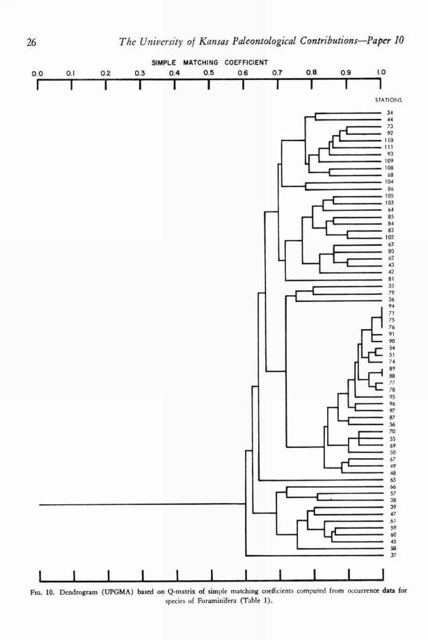
1 1 1 1 1 1 1 1 1 1 1FIG. 10. Dendrogram (UPGMA) based on Q-matrix of simple matching coefficients computed from occurrence data for
species of Foraminifera (Table 1).
Kaesler—Quantitative Re-evaluation in Todos Santos Bay, Mexico 27
example, cannot be attained unless each sample ina study has the same ecologic meaning. This clear-ly cannot be the case when sampling methods andsample sizes are not the same. Furthermore, iftotal population is used, even samples of equal sizecannot necessarily be considered equal in meaningbecause of transportation, mixing, and differentialdestruction of the dead population. Other criteriafor weighting have equally serious imperfections.
The equal weighting applies more readily toR-technique studies. If sampling is adequate andpresence-absence data are used, no problems shouldarise with the assumption. If abundance of speciesis to be considered, the investigator should collectsamples so that all have as nearly the same mean-ing as possible. In this study, the samples arenot necessarily the same in meaning, and noa priori basis exists for weighting. In the absenceof a basis for weighting, equal weighting ispreferable.
Assumptions 7) and 8) do not apply to bio-facies analysis to any great extent because a de-cision is usually made a priori about what taxa toinclude in a study. Every representative of thechosen taxa is then considered. Biofacies and bio-topes established as a result of the study will, ofcourse, depend on what taxa were used, sincedifferent groups of organisms need not have thesame distributions.
HYPOTHESES
Foul* hypotheses set up by SNEATH & SOKAL(1962, p. 4-6) to defend the assumptions are modi-fied below to apply to ecologic problems.
NEXUS HYPOTHESIS
The distribution of every species in a study islikely to be affected by more than one environ-mental factors. Conversely, most environmentalfactors affect the distribution of more than onespecies. Few ecologists would have any difficultyaccepting this hypothesis. GREIG-SMITH (1964, p.95) said:
In any community of more than a few species it isunlikely that an influencing factor will influence onespecies only, and the concurrent influence on severalspecies will result in association between them.
HYPOTHESIS OF NONSPECIFICITY
No large and distinct classes of environmentalfactors affect exclusively one species or a restricted
portion of a fauna. This hypothesis does not applyto biofacies analysis. It was proposed for numeri-cal taxonomy at a time when workers in that fieldwere perhaps more concerned with a real or finalclassification than now. Because the characters(species) in a numerical taxonomic biofacies
analysis of the type proposed here are fixed innumber and all possible characters are used in theanalysis, no difficulties can arise from lack of con-gruence of classifications.
HYPOTHESIS OF FACTOR ASYMPTOTE
This hypothesis makes three assertions(SNEATH 8c SOKAL, 1962, p. 5). 1) The morespecies studied the more information will be ac-cumulated, 2) A random sample of the speciesshould represent a random sample of the environ-mental factors acting in the area. 3) As more andmore species are included, the rate of gain of newinformation for classificatory purposes will de-crease. The hypothesis has only limited applica-bility to biofacies analysis. As pointed out above,the biofacies analyst is not concerned with howmany species to consider; he studies all species ofthe taxa under consideration which occur in thestudy area.
HYPOTHESIS OF MATCHES ASYMPTOTE
The similarity between two stations is ex-
pressed by the proportion of species in which they
agree. SNEATH & SOKAL (1962, p. 6), discussingthis hypothesis, wrote:
If we assume that we are making an estimate of aparametric value of matches of all possible charactersby using a sample of characters, we expect that thesimilarity coefficient would become more stable as thenumber of characters increases, and would eventuallyapproach that parametric proportion of matches whichwe would obtain if we were able to include all thecharacters. Further increase in the number of charac-ters is not warranted by the corresponding mild de-crease in the width of the confidence band of thecoefficient.
The parametric value in a monotaxic ecologic
study is the number of matches if all the organismsbelonging to the taxon in the study area have beenfound. If many samples have been taken fromdiverse environments within the study area, theactual number of matches should be very close tothe parametric value, particularly if total popula-tion is used so that seasonal variation is minimized.
28 The University of Kansas Paleontological Contributions—Paper 10JACCARD COEFFICIENT
0.0 0.1 0.2 0.3 0.4 0.5 0.6 0.7 0.8 0.9 1.0
1 1 1 1 1 1 1 1 1 1STATIONS
347393
11011144
35793766573865
10936
1088668
10510364858483
10281
10463806243
4294717576
9190748789887778959697
517055696750564948394745
59606192
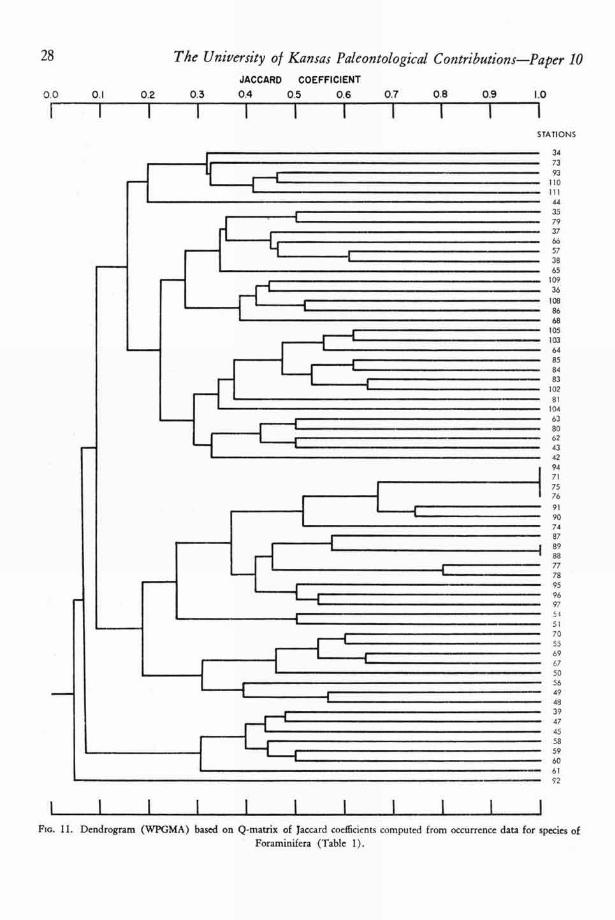
Flo. 11. Dendrogram (WPGMA) based on Q-matrix of Jaccard coefficients computed from occurrence data for species ofForaminifera (Table 1).
Kaesler—Quantitative Re-evaluation in Todos Santos Bay, Mexico 29
EVALUATION OF COEFFICIENTS
OF ASSOCIATION
CORRELATION COEFFICIENT
In biofacies analysis the correlation coefficientis computed from counts of specimens of eachspecies at all stations included in the study. Neces-sary to an evaluation of the usefulness of the co-efficient, then, is an evaluation of meaningfulnessof the data.
The use of numerical data such as those inTables 1 and 2, although it seems to give muchdetailed information, has several fundamental dis-advantages in ecologic work. JOHNSON (1960)gave an excellent discussion of the "circumstancesleading to the preservation of shallow-water ma-rine organisms." He listed (p. 1084) three char-acteristics of marine environments which causedeath assemblages to differ from life assemblagesand which introduce bias into paleoecologic work:1) Selectivity of destructive processes operatingupon death assemblages. 2) Mixing of indigenousand exotic elements in a death assemblage. 3) Phy-sical and chemical alteration of fossils and enclos-ing sediment.
Limitations of using total number of specimensin a sample for quantitative biofacies analysis werediscussed by IMBRIE (28, p. 653-654), who listedthe following kinds of information represented bythe total: specimens of all growth stages, brokenmaterial from groups of unequal fragility, andhard parts of organisms bearing various quantita-tive relations to soft anatomy. Each sample mayhave an entirely different ecologic meaning, andtotal number of specimens reflects at least fourfactors, the first three of which apply even if onlythe living population is considered in the study.1) Sample size. 2) Productivity. 3) Rate of sedi-mentation. 4) Rate of removal of dead materialby physical and chemical means.
If total number of organisms is not preciselymeaningful, then statistics derived from totalnumber can be of no more value. Specifically, useof number of species per unit weight or per unitvolume does not consider variance among sampleswith respect to the four factors listed.
The correlation coefficient, widely used innumerical taxonomic work presents other prob-lems in addition to those mentioned above whenapplied to ecologic problems. Discussing the Pear-son product-moment correlation coefficient, STEEL
& TORRIE (1960. p. 183) said: "It is assumed that,
in the population, a linear relation exists betweenthe variables. This is a valid assumption whensampling is from a bivariate normal distribution."COLE (1949, p. 422) stressed the limitations ofcorrelation methods in general because of the dis-tinctly " 'non-random' nature of the spatial dis-tributions commonly observed in populations oforganisms." This is certainly the case with thedata of this study, particularly the Ostracoda(Table 2). JoHNsoN (1962, p. 33-34) further ques-tioned the applicability of correlation statistics todelimit faunal associations (R-technique) beyondthe failure of the data to fit assumptions of themethod:
A correlation statistic may reflect other sorts of rela-tions . . . , but its use to delimit faunal association isopen to question. Two species may occur togetherfrequently and have no constant relationship betweentheir numbers. . . . This circumstance is too commonin marine communities to permit the use of a corre-lation statistic to represent faunal associations. Inpaleontological samples, the number of individuals ofa particular species is difficult to obtain and interpret.
In paleoecological work where the dead popu-lation or total population must be used as the bestavailable estimate of the live population, use ofnumerical data, such as number of specimens perspecies at a station, should be avoided. In a studyin which only the live population is considered forbiofacies analysis, actual counts may be used tocompute correlation coefficients if the populationsare normally distributed and the investigator hassome means of ascertaining the ecologic meaningof each sample.
Principal components factor analysis and rota-tion to simple structure using SOKAL ' S MTAMrotation (SoKAL, 1958) were done on foraminiferaland ostracodal R-technique correlation coefficients,regardless of the unreliability of the correlation co-efficients. The result of the factor analysis weremeaningless and are not reported here.
SIMPLE MATCHING COEFFICIENT
The simple matching coefficient was introducedinto numerical taxonomy by SoKAL & MICHENER
(1958), but it was used earlier by other workersfor other purposes (57, p. 133). It is calculated bythe equation:
a dSsm =
where a is the number of cases in which two com-pared items are both present, d the number of
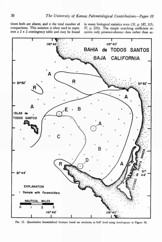
11116° 40'
• . BAHIA de TODOS SANTOS
• " • BAJA CALIFORNIA
116°40' :" •
: 1
1 1 • 1
116° 46'
•
-• 31° 52'
NINO
3p044'
Noon
NAUTICAL MILES1111111111111C=1M1111111111101 2 3
116°46'1
30
The University of Kansas Paleontological Contributions—Paper 10
times both are absent, and n the total number of in many biological statistics texts (51, p. 187, 315;comparisons. This notation is often used to repre- 57, p. 220). The simple matching coefficient re-sent a 2 x 2 contingency table and may be found quires only presence-absence data rather than ac-
Fin. 12. Quantitative foraminiferal biotopes based on similarity at 0.67 level using dendrogram in Figure 10.
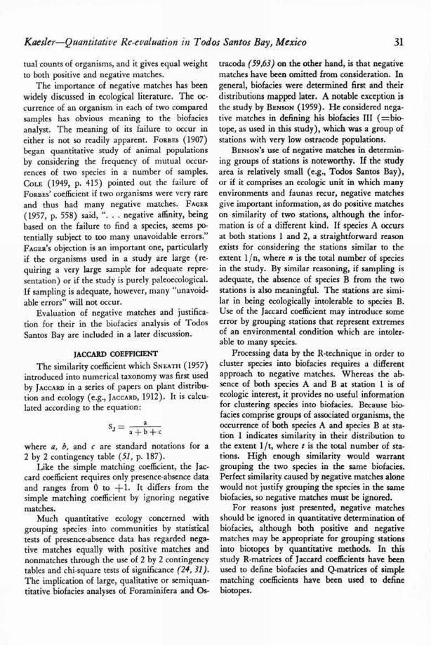
Kaesler—Quantitative Re-evaluation in Todos Santos Bay, Mexico 31
tuai counts of organisms, and it gives equal weightto both positive and negative matches.
The importance of negative matches has beenwidely discussed in ecological literature. The oc-currence of an organism in each of two comparedsamples has obvious meaning to the biofaciesanalyst. The meaning of its failure to occur ineither is not so readily apparent. FORBES (1907)began quantitative study of animal populationsby considering the frequency of mutual occur-rences of two species in a number of samples.COLE (1949, p. 415) pointed out the failure of
FORBES ' coefficient if two organisms were very rare
and thus had many negative matches. FAGER
(1957, p. 558) said, ". . . negative affinity, beingbased on the failure to find a species, seems po-tentially subject to too many unavoidable errors."PAGER ' S objection is an important one, particularlyif the organisms used in a study are large (re-quiring a very large sample for adequate repre-sentation) or if the study is purely paleoecological.
If sampling is adequate, however, many "unavoid-able errors" will not occur.
Evaluation of negative matches and justifica-tion for their in the biofacies analysis of TodosSantos Bay are included in a later discussion.
JACCARD COEFFICIENT
The similarity coefficient which SNEATH ( 1957)introduced into numerical taxonomy was first usedby LAGGARD in a series of papers on plant distribu-tion and ecology (e.g., JACCARD, 1912). It is calcu-lated according to the equation:
S T =a+b+ c
where a, b, and c are standard notations for a2 by 2 contingency table (51, p. 187).
Like the simple matching coefficient, the Jac-card coefficient requires only presence-absence dataand ranges from 0 to +1. It differs from thesimple matching coefficient by ignoring negativematches.
Much quantitative ecology concerned withgrouping species into communities by statisticaltests of presence-absence data has regarded nega-tive matches equally with positive matches andnonmatches through the use of 2 by 2 contingencytables and chi-square tests of significance (24, 31).
The implication of large, qualitative or semiquan-titative biofacies analyses of Foraminifera and Os-
tracoda (59,63) on the other hand, is that negativematches have been omitted from consideration. Ingeneral, biofacies were determined first and theirdistributions mapped later. A notable exception isthe study by BENSON (1959). He considered nega-tive matches in defining his biofacies III (=bio-tope, as used in this study), which was a group ofstations with very low ostracode populations.
BENSON'S use of negative matches in determin-ing groups of stations is noteworthy. If the studyarea is relatively small (e.g., Todos Santos Bay),or if it comprises an ecologic unit in which manyenvironments and faunas recur, negative matchesgive important information, as do positive matcheson similarity of two stations, although the infor-mation is of a different kind. If species A occursat both stations 1 and 2, a straightforward reasonexists for considering the stations similar to theextent 1/n, where n is the total number of speciesin the study. By similar reasoning, if sampling isadequate, the absence of species B from the twostations is also meaningful. The stations are simi-lar in being ecologically intolerable to species B.Use of the Jaccard coefficient may introduce someerror by grouping stations that represent extremesof an environmental condition which are intoler-able to many species.
Processing data by the R-technique in order tocluster species into biofacies requires a differentapproach to negative matches. Whereas the ab-sence of both species A and B at station 1 is ofecologic interest, it provides no useful informationfor clustering species into biofacies. Because bio-facies comprise groups of associated organisms, theoccurrence of both species A and species B at sta-tion 1 indicates similarity in their distribution tothe extent 1/t, where t is the total number of sta-tions. High enough similarity would warrantgrouping the two species in the same biofacies.Perfect similarity caused by negative matches alonewould not justify grouping the species in the samebiofacies, so negative matches must be ignored.
For reasons just presented, negative matchesshould be ignored in quantitative determination ofbiofacies, although both positive and negativematches may be appropriate for grouping stationsinto biotopes by quantitative methods. In thisstudy R-matrices of Jaccard coefficients have beenused to define biofacies and Q-matrices of simplematching coefficients have been used to definebiotopes.
a
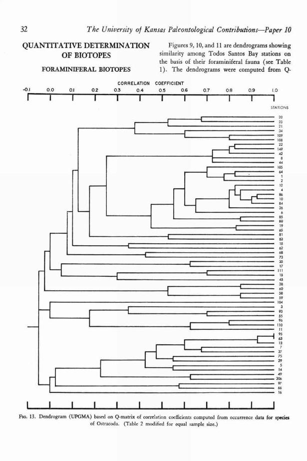
32 The University of Kansas Paleontological Contributions—Paper 10
QUANTITATIVE DETERMINATIONOF BIOTOPES
FORA MINIFERAL BIOTOPES
Figures 9, 10, and 11 are dendrograms showingsimilarity among Todos Santos Bay stations onthe basis of their foraminiferal fauna (see Table1). The dendrograms were computed from Q-
STATIONS
20232134
10910822
14942
844
10564
12
124
86108436
6858019658183186268733517
1 1 1154538605859
1043
935596
1101195
63137
377529
51449
306976616
I I Ino. 13. Dendrogram (UPGMA) based on Q-matrix of correlation coefficients computed from occurrence data for species
of Ostracoda. (Table 2 modified for equal sample size.)
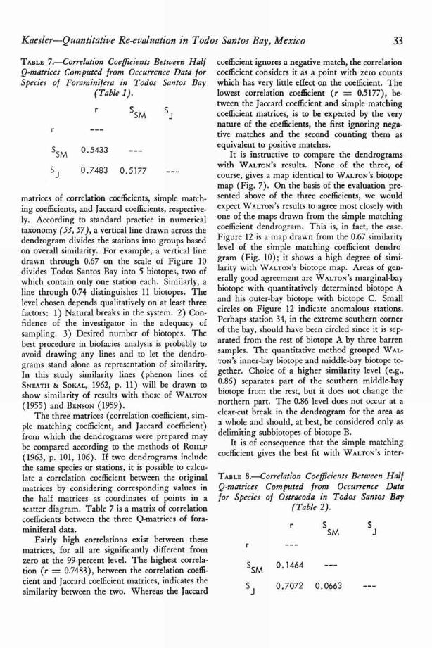
Kaesler—Quantitative Re-evaluation in Todos Santos Bay, Mexico 33
TABLE 7.—Correlation Coefficients Between HalfQ-matrices Computed from Occurrence Data forSpecies of Foraminif era in Todos Santos Bay
(Table I).
SM
SM 0.5433
0.7483 0.5177
matrices of correlation coefficients, simple match-ing coefficients, and Jaccard coefficients, respective-ly. According to standard practice in numericaltaxonomy (53, 57), a vertical line drawn across thedendrogram divides the stations into groups basedon overall similarity. For example, a vertical linedrawn through 0.67 on the scale of Figure 10divides Todos Santos Bay into 5 biotopes, two ofwhich contain only one station each. Similarly, aline through 0.74 distinguishes 11 biotopes. Thelevel chosen depends qualitatively on at least threefactors: 1) Natural breaks in the system. 2) Con-fidence of the investigator in the adequacy ofsampling. 3) Desired number of biotopes. Thebest procedure in biofacies analysis is probably toavoid drawing any lines and to let the dendro-grams stand alone as representation of similarity.In this study similarity lines (phenon lines ofSNEATH & SOKAL, 1962, p. 11) will be drawn toshow similarity of results with those of WALToN(1955) and BENSON (1959).
The three matrices (correlation coefficient, sim-ple matching coefficient, and Jaccard coefficient)from which the dendrograms were prepared maybe compared according to the methods of ROHLF(1963, p. 101, 106). If two dendrograms includethe same species or stations, it is possible to calcu-late a correlation coefficient between the originalmatrices by considering corresponding values inthe half matrices as coordinates of points in ascatter diagram. Table 7 is a matrix of correlationcoefficients between the three Q-matrices of fora-miniferal data.
Fairly high correlations exist between thesematrices, for all are significantly different fromzero at the 99-percent level. The highest correla-tion (r = 0.7483), between the correlation coeffi-cient and Jaccard coefficient matrices, indicates thesimilarity between the two. Whereas the Jaccard
coefficient ignores a negative match, the correlationcoefficient considers it as a point with zero countswhich has very little effect on the coefficient. Thelowest correlation coefficient (r 0.5177), be-tween the Jaccard coefficient and simple matchingcoefficient matrices, is to be expected by the verynature of the coefficients, the first ignoring nega-tive matches and the second counting them asequivalent to positive matches.
It is instructive to compare the dendrogramswith WALTON'S results. None of the three, ofcourse, gives a map identical to WALTON'S biotopemap (Fig. 7). On the basis of the evaluation pre-sented above of the three coefficients, we wouldexpect WALTON ' S results to agree most closely withone of the maps drawn from the simple matchingcoefficient dendrogram. This is, in fact, the case.Figure 12 is a map drawn from the 0.67 similaritylevel of the simple matching coefficient dendro-gram (Fig. 10); it shows a high degree of simi-larity with WALTON'S biotope map. Areas of gen-erally good agreement are WALTON ' S marginal-baybiotope with quantitatively determined biotope Aand his outer-bay biotope with biotope C. Smallcircles on Figure 12 indicate anomalous stations.Perhaps station 34, in the extreme southern cornerof the bay, should have been circled since it is sep-arated from the rest of biotope A by three barrensamples. The quantitative method grouped WAL-TON ' S inner-bay biotope and middle-bay biotope to-gether. Choice of a higher similarity level (e.g.,0.86) separates part of the southern middle-baybiotope from the rest, but it does not change thenorthern part. The 0.86 level does not occur at aclear-cut break in the dendrogram for the area asa whole and should, at best, be considered only asdelimiting subbiotopes of biotope B.
It is of consequence that the simple matchingcoefficient gives the best fit with WALTON ' S inter-
TABLE 8.—Correlation Coefficients Between HalfQ-matrices Computed from Occurrence Datafor Species of Ostracoda in Todos Santos Bay
(Table 2).
SM
sSM
0'1464
0.7072 0.0663
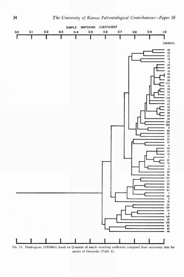
34 The University of Kansas Paleontological Contributions—Paper 10
SIMPLE MATCHING COEFFICIENT
0.0
0.1 0.2 0.3 0.4 0.5 0.6 0.7 0.8 0.9 1.0
iiiiiiiilSTATIONS 20 23 21
12 4E 22 49
16956366Ill
15935511
110 73 62
38605859
45 104 306 3 83 85 17 35 97 6
96 75
107
3713
5
14 29 36 105 64 80 84 81
682
1834
109198
14942
108866544
11111111111
t,Flo. 14. Dendrogram (UPGMA) based on Q-matrix of simple matching coefficients computed from occurrence data for
species of Ostracoda (Table 2).

Kaesler—Quantitative Re-evaluation in Todos Santos Bay, Mexico 35
pretation. As suggested above, the absence fromtwo stations of a species found elsewhere in thestudy area is an indication of similarity of environ-ment at the two stations. They are similar in theirunsuitability for the species in question, and thissimilarity contributes to their being clustered intothe same biotope. It would appear, then, that al-though WALTON delimited biofacies first in hisstudy and then mapped their distributions, he, aswell as BENSON, may have considered negativematches to be of some importance in clusteringstations into biotopes.
OSTRACODAL BIOTOPES
Figures 13, 14, and 15 are dendrograms pre-pared from Q-matrices of correlation coefficients,simple matching coefficients, and Jaccard coeffi-cients, respectively. The Q-matrices were com-puted from ostracode distribution data in Table 2.Because of the nature of the distribution of Ostra-coda over part of the study area, some assumptionsof biofacies analysis are not met, and none of thesedendrograms is believed to give a realistic repre-sentation of the biotopes in Todos Santos Bay.They are included here only for comparison.Table 8 gives the correlation coefficients betweenthe matrices.
Assumptions not satisfied are: 1) Biofacies andbiotopes exist in the study area. 2) Biotopes aremappable. BENSON found much of the central por-tion of the bay to be nearly barren of Ostracoda,and he grouped the stations in that area togetherinto a "barren biofacies" (=biotope). A so-calledbiofacies of this sort is a misnomer and does notexist in that area. Furthermore, the barren area isnot mappable by quantitative methods because ofthe nature of the data. Instead it is divided amongadjacent biotopes.
In order to meet all assumptions of biofaciesanalysis and to consider the barren area, all sta-tions with fewer than five ostracodes were tem-porarily omitted from the study. A Q-techniquesimple matching coefficient matrix was computedfrom that modified data matrix, and a dendrogram(Fig. 16) was prepared. A map (Fig. 17) showsthe quantitative biotopes at the 0.67 level.
Areas of general agreement with BENSON ' S re-sults (Fig. 8) are biotope A with parts of BENSON ' Sbiotope I and, of course, the barren area B withhis biotope Ill. An area of major disagreementexists between BENSON ' S biotope IV and the part
of quantitatively determined biotope A that lies indeeper water. Examination of the data in Table 2reveals that no stations in BENSON ' S biotope IVwere represented by more than a very few species,and only two of them were found at more thanone station. Clearly negative matches accountedfor the clustering of these stations with each other.All stations in the deep-water portion of biotopeA, except the shallowest (station 29), can be sep-arated from most of the rest of A at the 0.83 levelon the dendrogram (Fig. 14). The deep-waterportion, then, could be considered a subbiotope ofquantitative biotope A. Sampling in deep waterwas probably inadequate; if more Ostracoda hadbeen found at each station, the deep-water stationsmight have formed a separate biotope.
There are several stations which do not fit wellinto any pattern. Stations indicated as D and Emay be places of uniform environmental condi-tions that are not continuous. Biotope C nearlyeverywhere borders areas with a rocky substrate.If samples were collected in the rocky areas, wemight find that stations there could be groupedwith biotope C to form a rocky bottom biotope.
QUANTITATIVE DETERMINATIONOF BIOFACIES
FORAMINIFERAL BIOFACIES
Figures 18, 19, and 20 are dendrograms com-puted from R-matrices of correlation coefficients,simple matching coefficients, and Jaccard coeffi-cients, respectively, based on Table 1. They showsimilarity among species of Foraminifera based ontheir occurrence at stations in the study.
WALTON'S biofacies (Table 5) agree most close-ly with the Jaccard coefficient dendrogram. In par-ticular the 0.20 level gives very close agreementwith WALTON ' S subdivision of the fauna. This re-sult is what we would expect on the basis of theabove discussion of negative matches. It is en-couraging that field results agree with quantita-tively determined biofacies based on a coefficientthat excludes negative matches from consideration.Table 9 lists the major quantitatively determinedbiofacies based on the 0.20 level of the Jaccardcoefficient dendrogram. These should be com-pared with WALTON ' S biofacies listed in Table 5.
It must be remembered that WALTON ' S bio-facies concept allowed him to exclude some taxafrom any biofacies. Thus, not all taxa in the den-
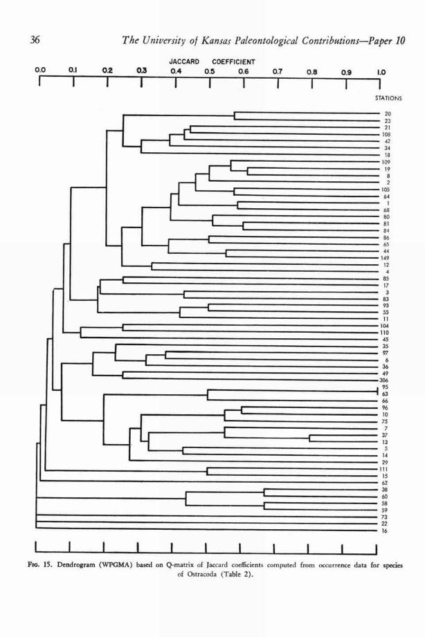
II 1 I I I I I I I IFIG. 15. Dendrogram (WPGMA) based on Q-matrix of Jaccard coefficients computed from occurrence data for species
of Ostracoda (Table 2).
JACCARD COEFFICIENT0.1 0.2 0.3 0.4 0.5 0.6 0.7 0.8 0.9 1.0
11 11111111
0.0
STATIONS
20 23 21 108 42 34
18109
198
2 105 64 1 68 80 81 84 86 65 44 149
124
85 17 3 83 93 55 11 104 110 45 35 97 6 36 49 306i 95I 63 66 96 10 75 7 37 13
5 14 29
1 1115
62 38 60 58 59 73 22 16
36 The University of Kansas Paleontological Contributions—Paper 10

Kaesler—Quantitative Re-evaluation in Todos Santos Bay, Mexico 37
SIMPLE MATCHING COEFFICIENT
0.0 0.1 0.2 0.3 0.4 0.5 0.6 0.7
0.8
0.9 1.0
1 1STATIONS
20232112
485
383808435
10411066455917 97 6 3 5 10 29
C 3713
36 105 64
811
68 2 18 34 109 42 108 19 8 149 44 86 65
Fic. 16. Dendrogram (WPGMA) based on Q-matrix of simple matching coefficients. The matrix was computed using
only those stations in Table 2 with five or more ostracodes after modification for equal-sample size.
drogram are included in his biofacies. Excludedtaxa fall into three categories: 1) Some largertaxa, such as Lagenidae, or general groupings,such as planktonic forms or unidentified forms.
TABLE 9. Quantitative Foraminiferal Bio facies
Based on 0.20 Level of laccard Coefficient Den -dro gram (Figure 20).
BIOFACIES AAmmotium planissimumGoesella ffintiiLabrospira sp. cf. L. advenaProteonina sp.Recurvoides spp.
Reophax curtusReophax scorpiurusUnidentified forms
BIOFACIES BBolivina acuminataBolivina pacificaBuccella frigidaBulimina denudataCancris auriculaGlobobulimina spp.LagenidaeReophax gracilisUvigerina peregrina subspp.
BIOFACIES CAngulogerfna angulosaCassidulina limbata

1 I 1116° 40'
BAHIA de TODOS SANTOS• BAJA CALIFORNIA
WIMP
MID
Wm*
WNW
1116° 46".;:: •
38
The University of Kansas Paleontological Contributions—Paper 10
Cassidulina tortuosa Cibicidina nitidulaCibicides fletcheri
Gaudryina sp. cf. G. subglabrataCibicides gallowayi
Polymorphinidae
Fic. 17. Quantitative ostracodal biotopes in Todos Santos Bay based on similarity at 0.67 level using dendrogram inFigure 16.
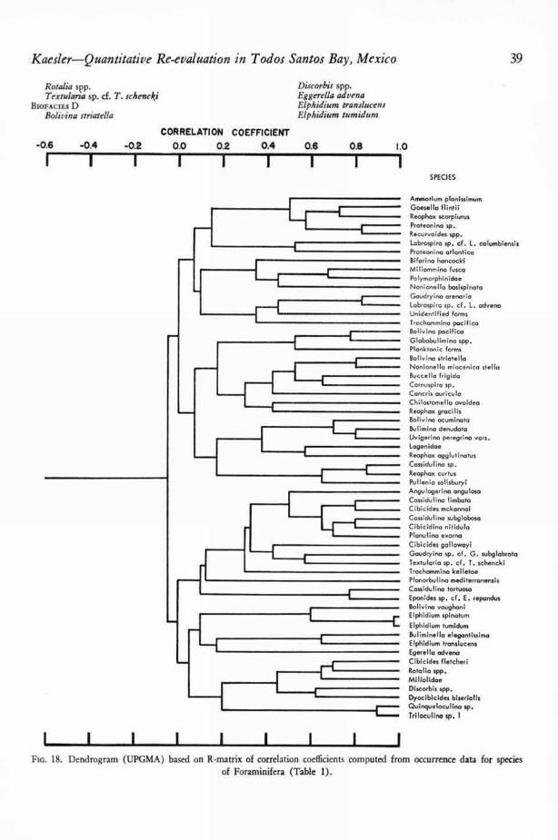
•Kaesler—Quantitative Re-evaluation in Todos Santos Bay, Mexico 39
Rotalia spp.Textularia sp. cf. T. schencki
BIOPACIES DRolivina striate/la
Discorbis spp.Eggerella adrenaElphidium translucentElphidium tumidum
CORRELATION COEFFICIENT-0.6 -0.4 -0.2 0.0 0.2 0.4 0.6 0.8 1.0
i1 1 11 11 1 IISPECIES
Ammotium planissimurn
Goesel la flintii
Reophax scorpiurus
Proteonina sp.
Recurvoides spp.
Labrospira sp. cf. L. columbiensis
Proteonina atlantic°
Bifarino hancocki
Miliammina fusca
P ly o ph'n'dae
Nonionella basispinato
Goudryino orenaria
Labrospira sp. cf. L. advenu
Unidentified forms
T ochornrnina pacifica
Bolivino pacific°
Globobulimina spp.
Planktonic forms
Bolivino striatello
Nonionello miocenica stello
Buccal la frigid° Cornuspiro sp.
C c is auricula
Chilostornello ovoidea
Reophax groci lis
Bolivino acuminota
Bulimina denudota
Uvigerina peregrina vars.Lagon doe
Reophax ogglutinatus
Cassidulino sp.
Reophax curtus
Pullenia solisburyi
Angulogerina anguloso
Cossidulina lirnbota
Cibicides mckannai
Cassidulina subglobosa
Cibicidina nitidula
Planulina exorno
Cibicides gal lowoyi
Goudryina sp. cf. G. subglabrata
Textularia sp. cf. T. schencki
Trochammina kelletae
Planorbulina mediterronensis
Cassidulina tortuoso
Eponides sp. cf. E. rependus
Bolivino vaughani
Elphidiurn spinotum
Elphidium turnidurn
Bulirninella elegantissima
Elphidium translucent Egerella advena
Cibicides fletcheri
Rotalia spp.
Mi I iolidae
Discorbis spp.
Dyocibicides biserialis
Quinqueloculina sp.
Triloculina sp. I
FIG. 18. Dendrogram (UPGMA) based on R-matrix of correlation coe fficients computed from occurrence data for speciesof Foraminifera (Table 1).
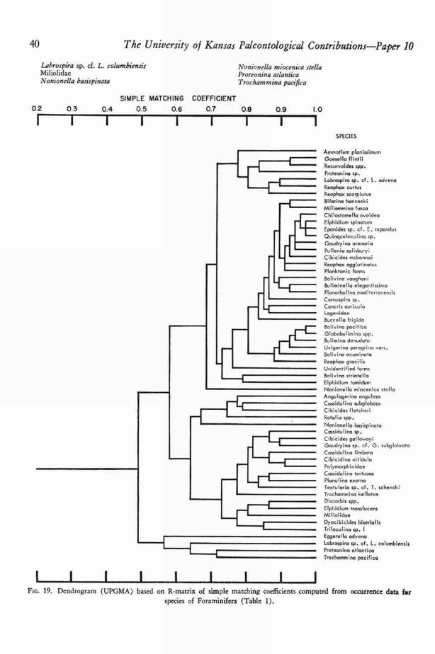
-r-'
40 The University of Kansas Paleontological Contributions—Paper 10
Labrospira sp. cf. L. columbiensis Nonionella miocenica stellaMiliolidae Proteonina atlanticaNonionella basispinata Trocham mina pacifica
SIMPLE MATCHING COEFFICIENT0.2 0.3 0.4 0.5 0.6 0.7 0.8 0.9 1.0
SPECIES
Ammotium planissimum
Goesel la flintii
Recurvoides spp.
Proteonina sp.
Labrospiro sp. cf. L. advene
Reophax curtus
Reophax scorpiurus
Bifarine hancocki
Miliammina fusca
Chi lostomella ovoidea
Elphidium spinatum
Eponides sp. cf. E. repandus
Quinqueloculina sp.
Gaudryino orenoria
Pullenia salisburyi
Cibicides mckannai
Reophox agglutinotus
Planktonic forms
Bolivino voughoni
Buliminella elegontissima
Plonorbulino rnediterranensis
Cornuspira sp.
Cancris ooricula
Logenidae
Buccello frigid°
Bolivina pocif ice
Globobulimina pp.
B I a derive:Iota
Uvigerina peregrine vars.
Bolivina acurninoto
Reophox gracilis
Unidentified forms
Bolivina striatel la
Elphidiurn turnidum
Nonionello rniocenico stella
Angulogerina angulosa
Cassidulina subgloboso
Cibicides fletcheri
Rotalia pp.
Nonionella basispinato
Cassidulina sp.
Cibicides gal lowayi
Gaudryina sp. cf. G. subglobrato
Cassidulina limboto
Cibicidina nitidula
Polyrnorphinidae
Cassidulina tortuoso
Planulina exorna
Textularia sp. cf. T. schencki
T ochammina kelletae
Discorbis pp.
Elphidium translucens
Miliolidae
Dyocibicides biserialis
Triloculina sp. I
Eggerello advena
Labrospira sp. cf. L. columbiensis
Proteonina otlantica
Trochammina pocifica
FIG. 19. Dendrogram (UPGMA) based on R-matrix of simple matching coefficients computed from occurrence data forspecies of Foraminifera (Table 1).

Kaesler—Quantitative Re-evaluation in Todos Santos Bay, Mexico 41
2) Species not restricted to a single biotope, such frtgida (CostalAll). 3) Species too rare in theas Trocham mina kelletae THALMANN and Buccella study area to be included in any biofacies, such as
JACCARD COEFFICIENT
0.0 0.2 0.4 0.6 0.8 1.0
SPECIES
Ammotium planissimum
Proteonina sp.
Goesella flintii
Recurvoides
Labrospira sp. cf. L. adveno
Reophax curtus
Reophax scorpiurus
Unidentified forms
Bolivina pacific°
Globobulimina spp.
Bulimina denudato
Uvigerina peregrina vars.
Bolivina ocuminato
Reophax grocilis
Concris auriculo
Buccello frigida
Logenidoe
Cornuspira sp.
Planktonic forms
Biforino hancocki
Miliammina Fusco
Angulogerina angulosa
Cibicides fletcheri
Rotolia
Cassidulino subglobosa
Planulino exorna
Cossidulino tortuosa
Textularia sp. cf. T. schencki
Cassidulina limbato
Cibicidina nitidulo
Polymorphinidoe
Cibicides gallowayi
Goudryina sp. cf. G. svbglobraia
T ochammino kelletoe
Cibicides rnckannai
Bolivina striotella
Nonionel la rniocenica 'tell°Nonionella bosispinota
Eggerella advena
Labrospira sp. cf. L. columbiensis
Proteonino atlantica
Trochammina pacifica
Elphidium tumidurn
Discorbis pp.
Elphidium tronstucens
Miliolidae
Triloculino sp. 1
Dyocibicides biserialis
Planorbulino mediterronensis
Buliminella elegantissima
Bolivino voughani
Elphidium spinatum
Gaudryina arenoria
Cassidulino sp.
Pullenia salisburyi
Reophax ogglutinatus
Quingueloculina sp.
Chilostornello ovoidea
Eponides sp. cf. E. repandus
Fm. 20. Dendrogram (WPGMA) based on R-matrix of jaccard coefficients computed from occurrence data for speciesof Foraminifera (Table 1).

42 The University of Kansas Paleontological Contributions—Paper 10
CORRELATION COE FFI CIENT
-0.6 -0.4 -0.2 0.0 0.2 0.4 0.6
0.8 1.0
SPECIES
Xestoleberis aurantia
Bradleyo (writ°
Paracypris pacific°
Genus A species A
Candîtes
C Bairdia sp. off. B. verdesens4
Cytherelloidea californica
Cythereis glauca
Brachycytkere sp.
Loxoconcha lenticular°
Hernicythere jol laensis
Brachycythere lincolnensis
Paracytheridea grossi
Bradley° diegoensis
Hemicythere sp. cf. H. clathrato
Basslerites delreyensis
Pellucistoma scrippsi
Quadracythere regalia
Haplocytheridea maia
Sclerochilus nasus
Triebelina reticulopunctata
B ochycythere driveri
Hemicythere coliforniensis
Cytheropteron newportense
Cytherura sp. cf. C. gibba
Cytherura bajocala
Legurninocythereis corrugate
Pterygocythereis sernitranslucens
Cytherello banda
B adleyo sp. cf. B. schencki
Palmanella carida
Bradley° pennata
Hemicytheridea sp.
Brachycythere schumannensis
Hemicythere polosensis
Bythocypris actites
Cytheropteron ensenadum
Cytheropteron pacificum
11FIG. 21. Dendrogram (UPGMA) based on R-matrix of correlation coefficients computed from occurrence data for species
of Ostracoda (Table 2).
Pullenia salisburyi STEWART & STEWART and Cibi-cides mckannai GALLOWAY & WISSLER.
Some of the species that WALToisi included inhis various biofacies are excluded or shown in adifferent one by the dendrogram. In other in-stances, species indicated as included in a biofaciesby the dendrogram were not included by WALTON.
These two cases are analogous to Type I and TypeII errors of statisticians (58, p. 70), although erroris not necessarily involved—only difference ofopinion. In general, species that the quantitativemethod places in what seems to be an incorrectbiofacies are rare in the study area (low counts) orthey occur at very few stations, or both.
Before basing biofacies on dendrograms alone,an investigator should compare the original data
and the dendrogram to look for species that areobvious exceptions to the presumed natural systemor that occur so rarely that they are clustered withothers only because of blind objectivity of themethod. Minor modifications of the quantitativeresults would be permissible under such circum-stances where the sample size is small and someassumptions of the quantitative method obviouslyare not met.
Table 10 is a matrix of correlation coefficientsbetween the three R-matrices. Correlation betweenthe correlation coefficient matrix and the simplematching coefficient matrix is low but significant.The very low correlation between the Jaccard co-efficient matrix and simple matching coefficientmatrix results from the diverse nature of the two

Kaesler—Quantitative Re-evaluation in Todos Santos Bay, Mexico 43
SIMPLE MATCHING COEFFICIENT
0.2 0.3 0.4 0.5 0.6 0.7 0.8
0.9 1.0
1 1 1SPECIES
Xestoleberis aurantia
Bradley° aurita
Hemicytheruro sp. cf. H. clathrota
Genus A species A
Brachycythere sp.
Paracypris pacific° Haplocytheridea naja
Quadracythere regaliaBairdia sp. off. B. verdesensis
Basslerites delreyensis
Pellucistorno scrippsi
Cytheropteron newportense
Cytheropteron pacificum
Hemicythere palosensis
Sclerochilus nasus
Triebelina reticulopunctata
Bythocypris actites
Cytheropteron ensenadurn
Brachycythere schumannensis
B adleya pennata
Hemicytheridea sp.
Caudites frogilis
Cytherura bajocala
Cytherelloidea californico
Cythereis glauca
Hemicythere jai laensis
Brachycythere driven i
Paracytheridea gronti
Bradley° sp. cf. B. schencki
Loxoconcha lenticular° Brachycythere lincolnensis
Bradley° diegoensis
Hemicythere coliforniensis
Cytherel la banda Cytherura sp. cf. C. gibba
Polmanella condo L guminocythereis corrugato
Pterygocythereis semitranslucens
1 1FIG. 22. Dendrogram (UPGMA) based on R-matrix of simple matching coefficients computed from occurrence data for
species of Ostracoda (Table 2).
TABLE 10.—Correlation Coefficients Between Half
R-Matrices Computed from Occurrence Data forSpecies of Foraminifera in Todos Santos Bay
(Table 1).
SM
SM 0.3170
0.6178 0.0519
coefficients. The higher correlation (r = 0.6178)between Jaccard and correlation coefficient mat-rices indicates the similarity between them. In-
spection of the dendrograms (Fig. 18-20) showsthat goodness of fit with WALTON 'S biofacies isroughly proportional to the value of the correlationcoefficients in row 3 of Table 10 if unity is enteredin the principal diagonal. Clearly, the simplematching coefficient dendrogram (Fig. 19) is thepoorest fit of the three; correlation coefficients givethe second best fit; and Jaccard coefficients give avery close fit.
OSTRACODAL BIOFACIES
Dendrograms based on occurrence data for os-tracode species (Table 2) are shown in Figures 21,22, and 23. The dendrograms were computedfrom R-matrices of correlation coefficients, simplematching coefficients, and Jaccard coefficients, re-
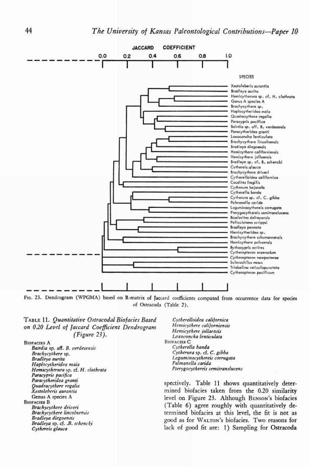
44 The University of Kansas Paleontological Contributions—Paper 10
JACCARD COEFFICIENT
0.0 0.2 0.4 0.6 0.8
1.0
I I 1SPECIES
I 1
Xestoleberis aurantia
Bradleya aurita
Hemicytherura sp. cf. H. clathrataGenus A species ABrachycythere sp.
Haplocytheridea male
Quadracythere regalia
Paracypris pacific°
Bairdia sp. off. B. verdesensis
Paracytheridea granti
Loxoconcha lenticulata
B achycythere lincolnensis
Bradley° diegoensis
Hemicythere coliforniensis
Hemicythere jollaensis
Bradleya sp. cf. B. schencki
Cythereis alauca
Brachycythere driveni
Cytherelloidea californica
Coudites fragilis
Cytherura bajacala
Cytherella banda
Cytherura sp. cf. C. gibba
Palmanella carida
Legurninocythereis corrugate
Pterygocythereis semitranslucens
Basslerites delreyensis
P Iluestoma scrippsi
Bradley° pennata
He ytheridea sp.
Brachycythere schumannensis
Hemicythere palosensis
Bythocypris actites
Cytheropteron ensenadum
Cytheropteron newportense
Sclerochilus nasus
T •ebelina reticulopunctata
Cytheropteron pacificum
Fin. 23. Dendrogram (WPGMA) based on R-matrix of Jaccard coefficients computed from occurrence data for speciesof Ostracoda (Table 2).
TABLE 11. Quantitative Ostracodal Bio facies Basedon 0.20 Level of laccard Coefficient Dendrogram
(Figure 23).BIOFACIES A
Bairdia sp. all. B. verdesensisBrachycythere sp.Bradleya auritaHaplocytheridea maiaHemicytherura sp. cf. H. clath rataParacy pris pacificaParacytheridea grantiQuadracythere regaliaXestoleberis aurantiaGenus A species A
BIOFACIES BBrachycythere driver;Brachycythere lincolnensisBradleya diegoensisBradleya sp. cf. .B. schenckiCythereis glauca
Cytherelloidea californicaHemicythere californiensisHemicythere jollaensisLoxoconcha lenticulata
BIOFACIES CCytherella bandaCytherura sp. cf. C. gibbaLeguminocythereis corrugataPalmanella caridaPterygocythereis semitranslucens
spectively. Table 11 shows quantitatively deter-mined biofacies taken from the 0.20 similaritylevel on Figure 23. Although BENSON ' S biofacies(Table 6) agree roughly with quantitatively de-termined biofacies at this level, the fit is not asgood as for WALTON'S biofacies. Two reasons forlack of good fit are: 1) Sampling for Ostracoda
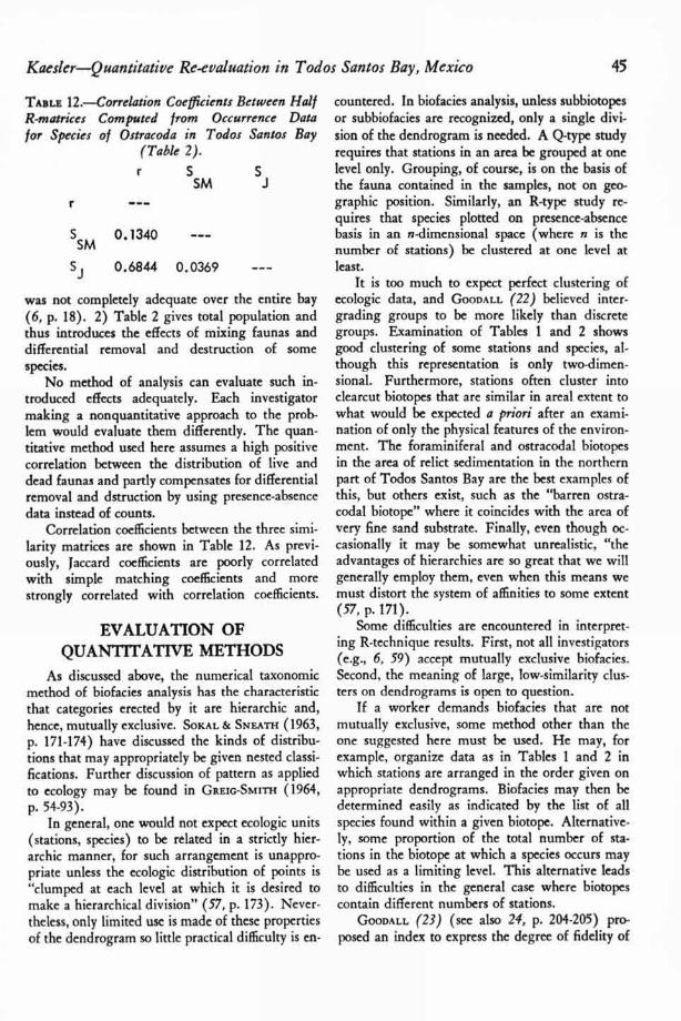
Kaeskr—Quantitative Re-evaluation in Todos Santos Bay, Mexico 45
TABLE 12.—Correlation Coefficients Between HalfR-matrices Computed from Occurrence Datafor Species of Ostracoda in Todos Santos Bay
(Table 2).
SM
S SM
0.1340
S 0.6844 0.0369
was not completely adequate over the entire bay(6, p. 18). 2) Table 2 gives total population andthus introduces the effects of mixing faunas anddifferential removal and destruction of somespecies.
No method of analysis can evaluate such in-troduced effects adequately. Each investigatormaking a nonquantitative approach to the prob-lem would evaluate them differently. The quan-titative method used here assumes a high positivecorrelation between the distribution of live anddead faunas and partly compensates for differentialremoval and dstruction by using presence-absencedata instead of counts.
Correlation coefficients between the three simi-larity matrices are shown in Table 12. As previ-ously, Jaccard coefficients are poorly correlatedwith simple matching coefficients and morestrongly correlated with correlation coefficients.
EVALUATION OFQUANTITATIVE METHODS
As discussed above, the numerical taxonomicmethod of biofacies analysis has the characteristicthat categories erected by it are hierarchic and,hence, mutually exclusive. SOKAL & SNEATH (1963,p. 171-174) have discussed the kinds of distribu-tions that may appropriately be given nested classi-fications. Further discussion of pattern as appliedto ecology may be found in GREIG-SMITH (1964,p. 54-93).
In general, one would not expect ecologic units(stations, species) to be related in a strictly hier-archic manner, for such arrangement is unappro-priate unless the ecologic distribution of points is"clumped at each level at which it is desired tomake a hierarchical division" (57, p. 173). Never-theless, only limited use is made of these propertiesof the dendrogram so little practical difficulty is en-
countered. In biofacies analysis, unless subbiotopesor subbiofacies are recognized, only a single divi-sion of the dendrogram is needed. A Q-type studyrequires that stations in an area be grouped at onelevel only. Grouping, of course, is on the basis ofthe fauna contained in the samples, not on geo-graphic position. Similarly, an R-type study re-quires that species plotted on presence-absencebasis in an n-dimensional space (where n is thenumber of stations) be clustered at one level atleast.
It is too much to expect perfect clustering ofecologic data, and GOODALL (22) believed inter-grading groups to be more likely than discretegroups. Examination of Tables 1 and 2 showsgood clustering of some stations and species, al-though this representation is only two-dimen-sional. Furthermore, stations often cluster intoclearcut biotopes that are similar in areal extent towhat would be expected a priori after an exami-nation of only the physical features of the environ-ment. The foraminiferal and ostracodal biotopesin the area of relict sedimentation in the northernpart of Todos Santos Bay are the best examples ofthis, but others exist, such as the "barren ostra-codal biotope" where it coincides with the area ofvery fine sand substrate. Finally, even though oc-casionally it may be somewhat unrealistic, "theadvantages of hierarchies are so great that we willgenerally employ them, even when this means wemust distort the system of affinities to some extent(57, p. 171).
Some difficulties are encountered in interpret-ing R-technique results. First, not all investigators(e.g., 6, 59) accept mutually exclusive biofacies.Second, the meaning of large, low-similarity clus-ters on dendrograms is open to question.
If a worker demands biofacies that are notmutually exclusive, some method other than theone suggested here must be used. He may, forexample, organize data as in Tables I and 2 inwhich stations are arranged in the order given onappropriate dendrograms. Biofacies may then bedetermined easily as indicated by the list of allspecies found within a given biotope. Alternative-ly, some proportion of the total number of sta-tions in the biotope at which a species occurs maybe used as a limiting level. This alternative leadsto difficulties in the general case where biotopescontain different numbers of stations.
GOODALL (23) (see also 24, p. 204-205) pro-posed an index to express the degree of fidelity of

EXPLANATION.---A. Biotope.---B. Species.---C. Chi-square.
---D. Probability.---E. Fidelity index,
A D
C Goesella flintii 1.5884 P .30 1.1778
C Recurvoides spp. 3.4455 P .10 1.3692
C Bolivina pacifica 26.2533 P .001 14.8333
C Globobulimina spp. 25.7610 P .001 41.5000
C Bulimina denudate 21.5874 P .001 36.5000
Uvigerina peregrina vars. 10.7188 P .01 8.1667
C Bolivina acuminate 12.3329 P .01 4.3571
C Reophax gracilis 16.5886 P .001 7.4000
C Cancris ouricula 1.3125 P .30 1.5000
C Buccella frigida 8.2031 P .01 4.5000
C Logenidae 1.3125 P .30 1.5000
A Cornuspira 1.6656 P .20 1.8000
A Cibicides fletcheri 8.2031 P .01 1.0000
A Rotalia spp. 8.3055 P .01 1.3059
C Cassidulina subglobosa 1.2635 P .30 0.2879
A Planulina exorna 2.4205 P .20 1.1600
A Cassidulina tortuosa 5.3293 P .05 8.2000
A Cassidulina limbata 1.2635 P .30 1.2667
A Cibicidina nitidula 3.1448 P .10 5.8000
A Gaudryina sp. cf. G. subglobosa 2.5318 P .20 5.0000
A Trochammina kelletae 2.4593 P .20 1.4000
C Bol vina striatello 1.8515 P .20 1.0455
C Nonionella miocenica stella 6.6500 P .01 1.2667
C Proteonina atlantic,, 7.3045 P .01 0.6204
B Trochammina pacific° 15.4006 P .001 1.0575
A Elphidium tumidum 1.5724 P .30 1.0800
A Discorbis spp. 3.2674 P .10 1.3644
A Elphidium translucens 2.4593 P .20 1.4000
A Miliolidae 6.3730 P .02 3.2560
A Triloculina sp. 1 1.2635 P .30 1.2667
A Dyocibicides biserialis 2.5318 P .20 5.0000
C Chilostomella ovoidea 2.2405 P .20 6.5000
46 The University of Kansas Paleontological Contributions-Paper 10
TABLE 13.-Species of Foraminifera in TodosSantos Bay with Fidelity Significant at 70-PercentLevel, Chi-Square Value, Significance Level, and
Fidelity Index.
plant species. The concept of fidelity as faithful-ness of a species to a certain community was sug-gested by BRAUN-BLANQUET (1951). Faithfulnessto a biotope may be expressed by the same index:
(a - Y2) (6 -E d)FIDELITY INDEX =
(6 -E. V2 ) (a -I- c)where a, b, c, and d are notation for a 2 x 2 con-tingency table, a is the number of occurrences inthe biotope where the species in question is mostfrequent, b its number of occurrences in the bio-tope in which it occurs next most commonly, andc and d are respective absences. At the same timefidelity-to-biotope may be tested for significancewith a chi-square test. Table 13 lists species ofForaminifera having a significant fidelity at the70-percent level with their corresponding fidelityindices and Table 14 gives similar information forOstracoda. Many other methods for groupingspecies into biofacies can be found. In each the
investigator must decide what criteria biofaciesrecognized by him must meet before he selects themethod. If mutual exclusiveness is desired, or notobjected to, the method presented in this study issuggested. (It is interesting to note that thespecies in Table 13 with highest fidelity are deep.water forms, suggesting transportation of shallow-water species into environments in which they arenot indigenous.)
The meaning of a cluster of two species havinga mutually highest Jaccard coefficient is that thetwo species tend to occur together to the extentindicated by the coe fficient. Similarly, specieswhich never join larger clusters or which do so ata similarity level too low to be meaningful aremost commonly species which occur at a very fewstations in the study area. Species which joinlarger clusters late but still at a meaningful levelare generally species that occur at a wider rangeof stations than others of the cluster (e.g., Tro-cham mina kelletae, Cibicides mckannai, Fig. 20)and that could be regarded as transitional in range.As new species are added to a cluster at increas-ingly low levels of similarity, the overall range ofstations occupied by the cluster as a whole, andthus, presumably, the range of tolerance to en-vironmental conditions, is increased. It is unfor-tunate that this method must place transitionalforms with one biofacies or another. I believe,however, that this characteristic is not a seriousdrawback to the method if one keeps in mind thenecessarily hierarchic nature of dendrograms. R-technique studies in ecology using the methods ofnumerical taxonomy will be much more meaning-ful if roughly the same quantitative biofacies areobtained from future studies of areas with similarspecies of Foraminifera and Ostracoda or otherorganic assemblages.
TABLE 14.-Species of Ostracoda in Todos SantosBay with Fidelity Significant at 70-Percent Level,Chi-Square Value, Significance Level, and Fidelity
Index.
EXPLANATION.---A. Biotope.---B. Species.---C. Chi-square.---D. Probability.---E. Fidelity index.
A D
D Xestoleberis aurantia 3.3750 P .10 1.8000D Haplocytheridea maia 1.5469 P .30 0.7500E Hemicythere californiensis 1.3645 P .30 0.4259C Cythereis glauca 5.7117 P .02 1.7238E Cytherella banda 5.4026 P .05 0.0000A Bythocypris actites 1.2036 P .30 0.0000A Cytheropteron newportense 1.2036 P .30 0.0000
Kaesler—Quantitative Re-evaluation in Todos Santos Bay, Mexico 47
CONCLUSIONSTodos Santos Bay and ecologic studies of Fora-
minifera and Ostracoda in this area provide excel-lent means of testing the applicability of methods
of numerical taxonomy to biofacies analysis. Onthe basis of preceding discussions, the followingconclusions are warranted.
1) For studies in which basic assumptions are
met and in which the study area behaves as anenvironmental unit with frequently recurring en-vironmental conditions and associations of or-ganisms, the methods of numerical taxonomy areconveniently applicable to problems of biofaciesanalysis.
2) Negative matches should be given equalweight with positive matches in forming biotopesif sampling is adequate and the study area behavesas an environmental unit (see conclusion 1). Den-drograms computed from Q-matrices of simplematching coefficients are suitable for definingquantitative biotopes.
3) Negative matches should be omitted fromconsideration in delimiting quantitative biofacies.Biofacies from dendrograms based on R-matricesof Jaccard coefficients are mutually exclusive. Ifone does not object to exclusivity in biofacies, den-drograms computed from R-matrices of Jaccardcoefficients are appropriate for biofacies.
4) Actual counts of organisms and use of cor-relation coefficients give moderately good resultsif only living populations are being studied and ifsamples are of nearly uniform size or ecologicmeaning. In studies involving total populations,unequal sizes of samples, or both, counts may bealmost entirely meaningless, as are statistics de-rived from the counts.
5) If populations are very small in part of thestudy area, nearly barren stations may be clusteredinto a barren area by temporarily omitting themfrom the study and proceeding with the reducedraw data matrix.
6) Different investigators use biofacies (and toa lesser extent, biotope) to express different con-cepts. The meaning adopted by WALTON (1955)and BFNSON (1959) is fairly clear, but this is cer-tainly not true in work published by others. Ef-fort should he made to determine what variouspaleoecologists mean by these terms to see by whatcriteria, quantitative or otherwise, and at whatsimilarity level they cluster species into hiofaciesand stations into biotopes.
7) Biofacies determined by the quantitativemethod of this study do not necessarily occupy bio-topes defined quantitatively. This does not meanthat these biofacies and biotopes are inherently dif-ferent from biofacies and biotopes determined bynonquantitative means. Indeed, the distinctionshould be avoided. Rather, one should recognizelack of congruence of biofacies and biotopes asinherent in the use of hierarchical classification,particularly where no obvious natural breaks occurin the classification.
The use of methods of numerical taxonomy inbiofacies analysis is not without disadvantages.Four disadvantages the user should rememberare:
1) The dendrogram is a two-dimensional rep-resentation of a multidimensional relationship.Some information is lost, particularly as one looksat larger clusters in a hierarchy, which are basedon lower similarity.
2) The simple matching coefficient indicateshigh similarity between stations at which only afew species are found, even if no species occurs atboth stations.
3) The numerical taxonomic method requiresa large study to reduce the effects of random error.It would be dangerous to place too much trust ina small study in which this method of analysiswas used. This objection applies particularly toR-technique studies.
4) This method of biofacies analysis formsmutually exclusive biotopes and biofacies; that is,it groups transitional species and stations into onebiofacies or another. One can, however, detecttransitional species from the dendrogram and rawdata matrix, so that the disadvantage of exclusivityis not a serious one.
No doubt other disadvantages will become ap-parent as the method is used in other areas and onother groups of organisms. To compensate fordisadvantages of the method and for cases inwhich assumptions are not met, the investigatormay make minor adjustments in his interpreta-tions. This procedure is not new to science, andcertainly not to geology. I believe disadvantagesof the method are outweighed by the advantages,which, restated, are: 1) Results are repeatable.2) Results are objective. 3) Computation of den-drograms is rapid. 4) Representation of results isgraphic. 5) Arbitrariness and relativity of thesimilarity level is not obscured.
Related Documents


