Package ‘Ecdat’ December 16, 2016 Version 0.3-1 Date 2016-12-15 Title Data Sets for Econometrics Author Yves Croissant <[email protected]> Maintainer Spencer Graves <[email protected]> Depends R (>= 2.10), Ecfun Suggests Description Data sets for econometrics. LazyData true License GPL (>= 2) URL https://www.r-project.org Repository CRAN Repository/R-Forge/Project ecdat Repository/R-Forge/Revision 389 Repository/R-Forge/DateTimeStamp 2016-12-15 15:40:54 Date/Publication 2016-12-16 02:19:24 NeedsCompilation no R topics documented: Accident ........................................... 4 Airline ............................................ 5 Airq ............................................. 6 bankingCrises ........................................ 7 Benefits ........................................... 8 Bids ............................................. 9 breaches ........................................... 10 BudgetFood ......................................... 12 BudgetItaly ......................................... 13 BudgetUK .......................................... 14 1

Welcome message from author
This document is posted to help you gain knowledge. Please leave a comment to let me know what you think about it! Share it to your friends and learn new things together.
Transcript
Package ‘Ecdat’December 16, 2016
Version 0.3-1
Date 2016-12-15
Title Data Sets for Econometrics
Author Yves Croissant <[email protected]>
Maintainer Spencer Graves <[email protected]>
Depends R (>= 2.10), Ecfun
SuggestsDescription Data sets for econometrics.
LazyData true
License GPL (>= 2)
URL https://www.r-project.org
Repository CRAN
Repository/R-Forge/Project ecdat
Repository/R-Forge/Revision 389
Repository/R-Forge/DateTimeStamp 2016-12-15 15:40:54
Date/Publication 2016-12-16 02:19:24
NeedsCompilation no
R topics documented:Accident . . . . . . . . . . . . . . . . . . . . . . . . . . . . . . . . . . . . . . . . . . . 4Airline . . . . . . . . . . . . . . . . . . . . . . . . . . . . . . . . . . . . . . . . . . . . 5Airq . . . . . . . . . . . . . . . . . . . . . . . . . . . . . . . . . . . . . . . . . . . . . 6bankingCrises . . . . . . . . . . . . . . . . . . . . . . . . . . . . . . . . . . . . . . . . 7Benefits . . . . . . . . . . . . . . . . . . . . . . . . . . . . . . . . . . . . . . . . . . . 8Bids . . . . . . . . . . . . . . . . . . . . . . . . . . . . . . . . . . . . . . . . . . . . . 9breaches . . . . . . . . . . . . . . . . . . . . . . . . . . . . . . . . . . . . . . . . . . . 10BudgetFood . . . . . . . . . . . . . . . . . . . . . . . . . . . . . . . . . . . . . . . . . 12BudgetItaly . . . . . . . . . . . . . . . . . . . . . . . . . . . . . . . . . . . . . . . . . 13BudgetUK . . . . . . . . . . . . . . . . . . . . . . . . . . . . . . . . . . . . . . . . . . 14
1

2 R topics documented:
Bwages . . . . . . . . . . . . . . . . . . . . . . . . . . . . . . . . . . . . . . . . . . . 15Capm . . . . . . . . . . . . . . . . . . . . . . . . . . . . . . . . . . . . . . . . . . . . 16Car . . . . . . . . . . . . . . . . . . . . . . . . . . . . . . . . . . . . . . . . . . . . . . 17Caschool . . . . . . . . . . . . . . . . . . . . . . . . . . . . . . . . . . . . . . . . . . 18Catsup . . . . . . . . . . . . . . . . . . . . . . . . . . . . . . . . . . . . . . . . . . . . 19Cigar . . . . . . . . . . . . . . . . . . . . . . . . . . . . . . . . . . . . . . . . . . . . 20Cigarette . . . . . . . . . . . . . . . . . . . . . . . . . . . . . . . . . . . . . . . . . . . 21Clothing . . . . . . . . . . . . . . . . . . . . . . . . . . . . . . . . . . . . . . . . . . . 22Computers . . . . . . . . . . . . . . . . . . . . . . . . . . . . . . . . . . . . . . . . . . 23Consumption . . . . . . . . . . . . . . . . . . . . . . . . . . . . . . . . . . . . . . . . 24CPSch3 . . . . . . . . . . . . . . . . . . . . . . . . . . . . . . . . . . . . . . . . . . . 25Cracker . . . . . . . . . . . . . . . . . . . . . . . . . . . . . . . . . . . . . . . . . . . 26CRANpackages . . . . . . . . . . . . . . . . . . . . . . . . . . . . . . . . . . . . . . . 27Crime . . . . . . . . . . . . . . . . . . . . . . . . . . . . . . . . . . . . . . . . . . . . 28CRSPday . . . . . . . . . . . . . . . . . . . . . . . . . . . . . . . . . . . . . . . . . . 29CRSPmon . . . . . . . . . . . . . . . . . . . . . . . . . . . . . . . . . . . . . . . . . . 30Diamond . . . . . . . . . . . . . . . . . . . . . . . . . . . . . . . . . . . . . . . . . . 31DM . . . . . . . . . . . . . . . . . . . . . . . . . . . . . . . . . . . . . . . . . . . . . 32Doctor . . . . . . . . . . . . . . . . . . . . . . . . . . . . . . . . . . . . . . . . . . . . 33DoctorAUS . . . . . . . . . . . . . . . . . . . . . . . . . . . . . . . . . . . . . . . . . 34DoctorContacts . . . . . . . . . . . . . . . . . . . . . . . . . . . . . . . . . . . . . . . 35Earnings . . . . . . . . . . . . . . . . . . . . . . . . . . . . . . . . . . . . . . . . . . . 36Electricity . . . . . . . . . . . . . . . . . . . . . . . . . . . . . . . . . . . . . . . . . . 37Fair . . . . . . . . . . . . . . . . . . . . . . . . . . . . . . . . . . . . . . . . . . . . . 38Fatality . . . . . . . . . . . . . . . . . . . . . . . . . . . . . . . . . . . . . . . . . . . 39FinancialCrisisFiles . . . . . . . . . . . . . . . . . . . . . . . . . . . . . . . . . . . . . 40Fishing . . . . . . . . . . . . . . . . . . . . . . . . . . . . . . . . . . . . . . . . . . . 41Forward . . . . . . . . . . . . . . . . . . . . . . . . . . . . . . . . . . . . . . . . . . . 42FriendFoe . . . . . . . . . . . . . . . . . . . . . . . . . . . . . . . . . . . . . . . . . . 43Garch . . . . . . . . . . . . . . . . . . . . . . . . . . . . . . . . . . . . . . . . . . . . 44Gasoline . . . . . . . . . . . . . . . . . . . . . . . . . . . . . . . . . . . . . . . . . . . 45Griliches . . . . . . . . . . . . . . . . . . . . . . . . . . . . . . . . . . . . . . . . . . . 46Grunfeld . . . . . . . . . . . . . . . . . . . . . . . . . . . . . . . . . . . . . . . . . . . 47HC . . . . . . . . . . . . . . . . . . . . . . . . . . . . . . . . . . . . . . . . . . . . . . 48Heating . . . . . . . . . . . . . . . . . . . . . . . . . . . . . . . . . . . . . . . . . . . 49Hedonic . . . . . . . . . . . . . . . . . . . . . . . . . . . . . . . . . . . . . . . . . . . 50HHSCyberSecurityBreaches . . . . . . . . . . . . . . . . . . . . . . . . . . . . . . . . 51HI . . . . . . . . . . . . . . . . . . . . . . . . . . . . . . . . . . . . . . . . . . . . . . 53Hmda . . . . . . . . . . . . . . . . . . . . . . . . . . . . . . . . . . . . . . . . . . . . 54Housing . . . . . . . . . . . . . . . . . . . . . . . . . . . . . . . . . . . . . . . . . . . 55Hstarts . . . . . . . . . . . . . . . . . . . . . . . . . . . . . . . . . . . . . . . . . . . . 56Icecream . . . . . . . . . . . . . . . . . . . . . . . . . . . . . . . . . . . . . . . . . . . 57incomeInequality . . . . . . . . . . . . . . . . . . . . . . . . . . . . . . . . . . . . . . 58IncomeUK . . . . . . . . . . . . . . . . . . . . . . . . . . . . . . . . . . . . . . . . . . 63Index.Econometrics . . . . . . . . . . . . . . . . . . . . . . . . . . . . . . . . . . . . . 64Index.Economics . . . . . . . . . . . . . . . . . . . . . . . . . . . . . . . . . . . . . . 66Index.Observations . . . . . . . . . . . . . . . . . . . . . . . . . . . . . . . . . . . . . 69Index.Source . . . . . . . . . . . . . . . . . . . . . . . . . . . . . . . . . . . . . . . . 72
R topics documented: 3
Index.Time.Series . . . . . . . . . . . . . . . . . . . . . . . . . . . . . . . . . . . . . . 76Irates . . . . . . . . . . . . . . . . . . . . . . . . . . . . . . . . . . . . . . . . . . . . 77Journals . . . . . . . . . . . . . . . . . . . . . . . . . . . . . . . . . . . . . . . . . . . 78Kakadu . . . . . . . . . . . . . . . . . . . . . . . . . . . . . . . . . . . . . . . . . . . 79Ketchup . . . . . . . . . . . . . . . . . . . . . . . . . . . . . . . . . . . . . . . . . . . 81Klein . . . . . . . . . . . . . . . . . . . . . . . . . . . . . . . . . . . . . . . . . . . . 82LaborSupply . . . . . . . . . . . . . . . . . . . . . . . . . . . . . . . . . . . . . . . . 83Labour . . . . . . . . . . . . . . . . . . . . . . . . . . . . . . . . . . . . . . . . . . . . 84Longley . . . . . . . . . . . . . . . . . . . . . . . . . . . . . . . . . . . . . . . . . . . 84LT . . . . . . . . . . . . . . . . . . . . . . . . . . . . . . . . . . . . . . . . . . . . . . 85Macrodat . . . . . . . . . . . . . . . . . . . . . . . . . . . . . . . . . . . . . . . . . . 86Males . . . . . . . . . . . . . . . . . . . . . . . . . . . . . . . . . . . . . . . . . . . . 87ManufCost . . . . . . . . . . . . . . . . . . . . . . . . . . . . . . . . . . . . . . . . . 88Mathlevel . . . . . . . . . . . . . . . . . . . . . . . . . . . . . . . . . . . . . . . . . . 89MCAS . . . . . . . . . . . . . . . . . . . . . . . . . . . . . . . . . . . . . . . . . . . . 90MedExp . . . . . . . . . . . . . . . . . . . . . . . . . . . . . . . . . . . . . . . . . . . 91Metal . . . . . . . . . . . . . . . . . . . . . . . . . . . . . . . . . . . . . . . . . . . . 92Mishkin . . . . . . . . . . . . . . . . . . . . . . . . . . . . . . . . . . . . . . . . . . . 93Mode . . . . . . . . . . . . . . . . . . . . . . . . . . . . . . . . . . . . . . . . . . . . 94ModeChoice . . . . . . . . . . . . . . . . . . . . . . . . . . . . . . . . . . . . . . . . . 95Mofa . . . . . . . . . . . . . . . . . . . . . . . . . . . . . . . . . . . . . . . . . . . . . 96Money . . . . . . . . . . . . . . . . . . . . . . . . . . . . . . . . . . . . . . . . . . . . 97MoneyUS . . . . . . . . . . . . . . . . . . . . . . . . . . . . . . . . . . . . . . . . . . 98Mpyr . . . . . . . . . . . . . . . . . . . . . . . . . . . . . . . . . . . . . . . . . . . . 99Mroz . . . . . . . . . . . . . . . . . . . . . . . . . . . . . . . . . . . . . . . . . . . . . 100MunExp . . . . . . . . . . . . . . . . . . . . . . . . . . . . . . . . . . . . . . . . . . . 101MW . . . . . . . . . . . . . . . . . . . . . . . . . . . . . . . . . . . . . . . . . . . . . 102NaturalPark . . . . . . . . . . . . . . . . . . . . . . . . . . . . . . . . . . . . . . . . . 103Nerlove . . . . . . . . . . . . . . . . . . . . . . . . . . . . . . . . . . . . . . . . . . . 104nonEnglishNames . . . . . . . . . . . . . . . . . . . . . . . . . . . . . . . . . . . . . . 105OFP . . . . . . . . . . . . . . . . . . . . . . . . . . . . . . . . . . . . . . . . . . . . . 105Oil . . . . . . . . . . . . . . . . . . . . . . . . . . . . . . . . . . . . . . . . . . . . . . 107Orange . . . . . . . . . . . . . . . . . . . . . . . . . . . . . . . . . . . . . . . . . . . . 108Participation . . . . . . . . . . . . . . . . . . . . . . . . . . . . . . . . . . . . . . . . . 109PatentsHGH . . . . . . . . . . . . . . . . . . . . . . . . . . . . . . . . . . . . . . . . . 110PatentsRD . . . . . . . . . . . . . . . . . . . . . . . . . . . . . . . . . . . . . . . . . . 111PE . . . . . . . . . . . . . . . . . . . . . . . . . . . . . . . . . . . . . . . . . . . . . . 112politicalKnowledge . . . . . . . . . . . . . . . . . . . . . . . . . . . . . . . . . . . . . 113Pound . . . . . . . . . . . . . . . . . . . . . . . . . . . . . . . . . . . . . . . . . . . . 115PPP . . . . . . . . . . . . . . . . . . . . . . . . . . . . . . . . . . . . . . . . . . . . . 116Pricing . . . . . . . . . . . . . . . . . . . . . . . . . . . . . . . . . . . . . . . . . . . . 117Produc . . . . . . . . . . . . . . . . . . . . . . . . . . . . . . . . . . . . . . . . . . . . 118PSID . . . . . . . . . . . . . . . . . . . . . . . . . . . . . . . . . . . . . . . . . . . . . 119RetSchool . . . . . . . . . . . . . . . . . . . . . . . . . . . . . . . . . . . . . . . . . . 120Schooling . . . . . . . . . . . . . . . . . . . . . . . . . . . . . . . . . . . . . . . . . . 121Solow . . . . . . . . . . . . . . . . . . . . . . . . . . . . . . . . . . . . . . . . . . . . 123Somerville . . . . . . . . . . . . . . . . . . . . . . . . . . . . . . . . . . . . . . . . . . 124SP500 . . . . . . . . . . . . . . . . . . . . . . . . . . . . . . . . . . . . . . . . . . . . 125
4 Accident
Star . . . . . . . . . . . . . . . . . . . . . . . . . . . . . . . . . . . . . . . . . . . . . 125Strike . . . . . . . . . . . . . . . . . . . . . . . . . . . . . . . . . . . . . . . . . . . . 126StrikeDur . . . . . . . . . . . . . . . . . . . . . . . . . . . . . . . . . . . . . . . . . . 127StrikeNb . . . . . . . . . . . . . . . . . . . . . . . . . . . . . . . . . . . . . . . . . . . 128SumHes . . . . . . . . . . . . . . . . . . . . . . . . . . . . . . . . . . . . . . . . . . . 129Tbrate . . . . . . . . . . . . . . . . . . . . . . . . . . . . . . . . . . . . . . . . . . . . 130terrorism . . . . . . . . . . . . . . . . . . . . . . . . . . . . . . . . . . . . . . . . . . . 131Tobacco . . . . . . . . . . . . . . . . . . . . . . . . . . . . . . . . . . . . . . . . . . . 135Train . . . . . . . . . . . . . . . . . . . . . . . . . . . . . . . . . . . . . . . . . . . . . 136TranspEq . . . . . . . . . . . . . . . . . . . . . . . . . . . . . . . . . . . . . . . . . . 137Treatment . . . . . . . . . . . . . . . . . . . . . . . . . . . . . . . . . . . . . . . . . . 138Tuna . . . . . . . . . . . . . . . . . . . . . . . . . . . . . . . . . . . . . . . . . . . . . 139UnempDur . . . . . . . . . . . . . . . . . . . . . . . . . . . . . . . . . . . . . . . . . 140Unemployment . . . . . . . . . . . . . . . . . . . . . . . . . . . . . . . . . . . . . . . 141University . . . . . . . . . . . . . . . . . . . . . . . . . . . . . . . . . . . . . . . . . . 142USclassifiedDocuments . . . . . . . . . . . . . . . . . . . . . . . . . . . . . . . . . . . 143USFinanceIndustry . . . . . . . . . . . . . . . . . . . . . . . . . . . . . . . . . . . . . 144USGDPpresidents . . . . . . . . . . . . . . . . . . . . . . . . . . . . . . . . . . . . . . 146USstateAbbreviations . . . . . . . . . . . . . . . . . . . . . . . . . . . . . . . . . . . . 150UStaxWords . . . . . . . . . . . . . . . . . . . . . . . . . . . . . . . . . . . . . . . . . 151VietNamH . . . . . . . . . . . . . . . . . . . . . . . . . . . . . . . . . . . . . . . . . . 153VietNamI . . . . . . . . . . . . . . . . . . . . . . . . . . . . . . . . . . . . . . . . . . 154Wages . . . . . . . . . . . . . . . . . . . . . . . . . . . . . . . . . . . . . . . . . . . . 155Wages1 . . . . . . . . . . . . . . . . . . . . . . . . . . . . . . . . . . . . . . . . . . . 156Workinghours . . . . . . . . . . . . . . . . . . . . . . . . . . . . . . . . . . . . . . . . 157Yen . . . . . . . . . . . . . . . . . . . . . . . . . . . . . . . . . . . . . . . . . . . . . 158Yogurt . . . . . . . . . . . . . . . . . . . . . . . . . . . . . . . . . . . . . . . . . . . . 159
Index 161
Accident Ship Accidents
Description
a cross-section
number of observations : 40
Usage
data(Accident)
Airline 5
Format
A dataframe containing :
type ship type, a factor with levels (A,B,C,D,E)constr year constructed, a factor with levels (C6064,C6569,C7074,C7579)operate year operated, a factor with levels (O6074,O7579)months measure of service amountacc accidents
Source
McCullagh, P. and J. Nelder (1983) Generalized linear methods, New York:Chapman and Hall.
References
Greene, W.H. (2003) Econometric Analysis, Prentice Hall, http://www.prenhall.com/greene/greene1.html, Table F21.3.
See Also
Index.Source, Index.Economics, Index.Econometrics, Index.Observations
Airline Cost for U.S. Airlines
Description
a panel of 6 observations from 1970 to 1984
number of observations : 90
observation : production units
country : United States
Usage
data(Airline)
Format
A dataframe containing :
airline airlineyear yearcost total cost, in \$1,000output output, in revenue passenger miles, index numberpf fuel pricelf load factor, the average capacity utilization of the fleet
6 Airq
References
Greene, W.H. (2003) Econometric Analysis, Prentice Hall, http://www.prenhall.com/greene/greene1.html, Table F7.1.
See Also
Index.Source, Index.Economics, Index.Econometrics, Index.Observations,
Index.Time.Series
Airq Air Quality for Californian Metropolitan Areas
Description
a cross-section from 1972
number of observations : 30
observation : regional
country : United States
Usage
data(Airq)
Format
A dataframe containing :
airq indicator of air quality (the lower the better)
vala value added of companies (in thousands of dollars)
rain amount of rain (in inches)
coas is it a coastal area ?
dens population density (per square mile)
medi average income per head (in US dollars)
References
Verbeek, Marno (2004) A Guide to Modern Econometrics, John Wiley and Sons, chapter 4.
See Also
Index.Source, Index.Economics, Index.Econometrics, Index.Observations

bankingCrises 7
bankingCrises Countries in Banking Crises
Description
A data.frame identifying which of 70 countries had a banking crisis each year 1800:2010. Thefirst column is year. The remaining columns carry the names of the countries; those columns are 1for years with banking crises and 0 otherwise.
Usage
data(bankingCrises)
Format
A data.frame
Details
This file was created using the following command:
bankingCrises <- readFinancialCrisisFiles(FinancialCrisisFiles)
This is documented further in the help file for readFinancialCrisisFiles.
This is an update of a subset of the data used to create Figure 10.1. Capital Mobility and theIncidence of Banking Crises, All Countries, 1800-2008, Reinhart and Rogoff (2009, p. 156).
The general upward trend visible in a plot of these data may be attributed to at least two differentfactors:
(1) The gradual increase in the proportion of human labor that is monetized.
(2) An increase in the general ability of cronies of those in power to gamble with other people’smoney in forming and bankrupting financial institutions. The marked feature of this plot is thevirtual absence of banking crises during the period of the Bretton Woods agreement, 1944 to 1971.This period ended when US President Nixon in effect canceled the Bretton Woods agreement bytaking the US off the silver standard.
Author(s)
Spencer Graves
Source
http://www.reinhartandrogoff.com
References
Carmen M. Reinhart and Kenneth S. Rogoff (2009) This Time Is Different: Eight Centuries ofFinancial Folly, Princeton U. Pr.
8 Benefits
See Also
readFinancialCrisisFiles
Examples
data(bankingCrises)numberOfCrises <- rowSums(bankingCrises[-1], na.rm=TRUE)plot(bankingCrises$year, numberOfCrises, type='b')
# Write to a file for Wikimedia Commonssvg('bankingCrises.svg')plot(bankingCrises$year, numberOfCrises, type='b', cex.axis=2,
las=1, xlab='', ylab='', bty='n', cex=0.5)abline(v=c(1945, 1971), lty='dashed', col='blue')text(1958, 14, 'Bretton Woods', srt=90, cex=2, col='blue')dev.off()
Benefits Unemployment of Blue Collar Workers
Description
a cross-section from 1972
number of observations : 4877
observation : individuals
country : United States
Usage
data(Benefits)
Format
A time serie containing :
stateur state unemployment rate (in %)
statemb state maximum benefit level
state state of residence code
age age in years
tenure years of tenure in job lost
joblost a factor with levels (slack\_work,position\_abolished,seasonal\_job\_ended,other)
nwhite non-white ?
school12 more than 12 years of school ?
sex a factor with levels (male,female)
Bids 9
bluecol blue collar worker ?
smsa lives is smsa ?
married married ?
dkids has kids ?
dykids has young kids (0-5 yrs) ?
yrdispl year of job displacement (1982=1,..., 1991=10)
rr replacement rate
head is head of household ?
ui applied for (and received) UI benefits ?
Source
McCall, B.P. (1995) “The impact of unemployment insurance benefit levels on recipiency”, Journalof Business and Economic Statistics, 13, 189–198.
References
Verbeek, Marno (2004) A Guide to Modern Econometrics, John Wiley and Sons, chapter 7.
Journal of Business Economics and Statistics web site : http://amstat.tandfonline.com/loi/ubes20.
See Also
Index.Source, Index.Economics, Index.Econometrics, Index.Observations,
Index.Time.Series
Bids Bids Received By U.S. Firms
Description
a cross-section
number of observations : 126
observation : production units
country : United States
Usage
data(Bids)

10 breaches
Format
A dataframe containing :
docno doc no.
weeks weeks
numbids count
takeover delta (1 if taken over)
bidprem bid Premium
insthold institutional holdings
size size measured in billions
leglrest legal restructuring
rearest real restructuring
finrest financial restructuring
regulatn regulation
whtknght white knight
Source
Jaggia, Sanjiv and Satish Thosar (1993) “Multiple Bids as a Consequence of Target ManagementResistance”, Review of Quantitative Finance and Accounting, 447–457.
Cameron, A.C. and Per Johansson (1997) “Count Data Regression Models using Series Expansions:with Applications”, Journal of Applied Econometrics, 12, may, 203–223.
References
Cameron, A.C. and Trivedi P.K. (1998) Regression analysis of count data, Cambridge UniversityPress, http://cameron.econ.ucdavis.edu/racd/racddata.html, chapter 5.
Journal of Applied Econometrics data archive : http://qed.econ.queensu.ca/jae/.
See Also
Index.Source, Index.Economics, Index.Econometrics, Index.Observations
breaches Cyber Security Breaches
Description
data.frame of cyber security breaches involving health care records of 500 or more humans re-ported to the U.S. Department of Health and Human Services (HHS) as of June 27, 2014.
Usage
data(breaches)
breaches 11
Format
A data.frame with 1055 observations on the following 24 variables:
Number integer record number in the HHS data base
Name_of_Covered_Entity factor giving the name of the entity experiencing the breach
State Factor giving the 2-letter code of the state where the breach occurred. This has 52 levels forthe 50 states plus the District of Columbia (DC) and Puerto Rico (PR).
Business_Associate_Involved Factor giving the name of a subcontractor (or blank) associated withthe breach.
Individuals_Affected integer number of humans whose records were compromised in the breach.This is 500 or greater; U.S. law requires reports of breaches involving 500 or more records butnot of breaches involving fewer.
Date_of_Breach character vector giving the date or date range of the breach. Recodes as Datesin breach_start and breach_end.
Type_of_Breach factor with 29 levels giving the type of breach (e.g., "Theft" vs., "UnauthorizedAccess/Disclosure", etc.)
Location_of_Breached_Information factor with 41 levels coding the location from which thebreach occurred (e.g., "Paper", "Laptop", etc.)
Date_Posted_or_Updated Date the information was posted to the HHS data base or last updated.
Summary character vector of a summary of the incident.
breach_start Date of the start of the incident = first date given in Date_of_Breach above.breach_end Date of the end of the incident or NA if only one date is given in Date_of_Breachabove.year integer giving the year of the breach
Details
The data primarily consists of breaches that occurred from 2010 through early 2014 when the extractwas taken. However, a few breaches are recorded including 1 from 1997, 8 from 2002-2007, 13from 2008 and 56 from 2009. The numbers of breaches from 2010 - 2014 are 211, 229, 227, 254and 56, respectively. (A chi-square test for equality of the counts from 2010 through 2013 is 4.11,which with 3 degrees of freedom has a significance probability of 0.25. Thus, even though thelowest number is the first and the largest count is the last, the apparent trend is not statisticallysignificant under the usual assumption of independent Poisson trials.)
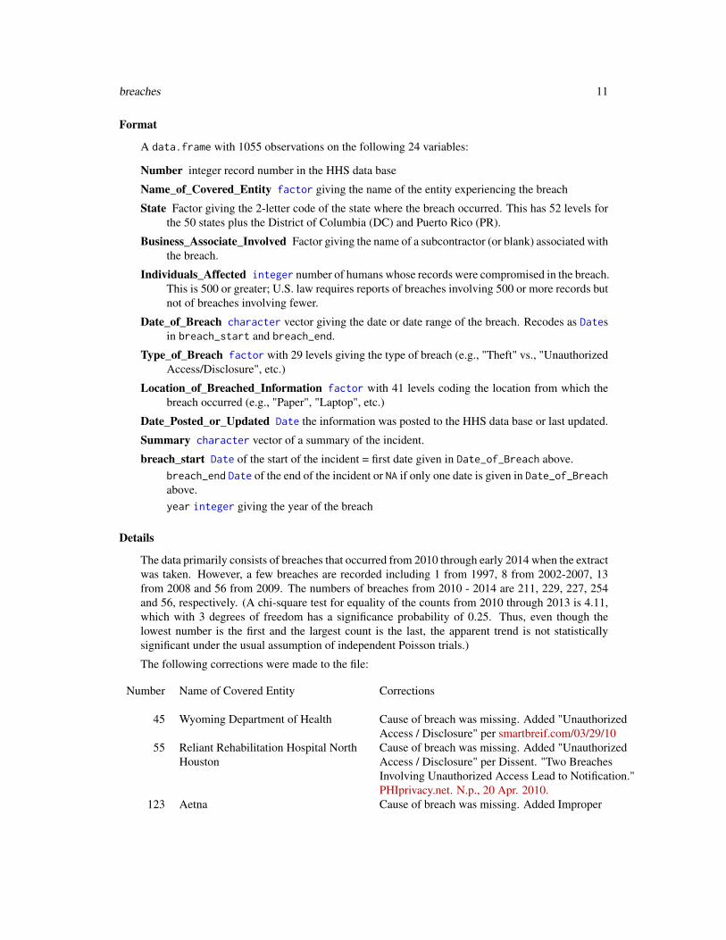
The following corrections were made to the file:
Number Name of Covered Entity Corrections
45 Wyoming Department of Health Cause of breach was missing. Added "UnauthorizedAccess / Disclosure" per smartbreif.com/03/29/10
55 Reliant Rehabilitation Hospital North Cause of breach was missing. Added "UnauthorizedHouston Access / Disclosure" per Dissent. "Two Breaches
Involving Unauthorized Access Lead to Notification."PHIprivacy.net. N.p., 20 Apr. 2010.
123 Aetna Cause of breach was missing. Added Improper

12 BudgetFood
disposal per Aetna.com/news/newsReleases/2010/0630157 Mayo Clinic Cause of breach was missing. Added Unauthorized
Access/Disclosure per Anderson, Howard. "Mayo Fires"Employees in 2 Incidents: Both InvolvedUnauthorized Access to Records."Data Breach Today. N.p., 4 Oct. 2010
341 Saint Barnabas MedicL Center Misspelled "Saint Barnabas Medical Center"347 Americar Health Medicare Misspelled "American Health Medicare"484 Lake Granbury Medicl Ceter Misspelled "Lake Granbury Medical Center"782 See list of Practices under Item 9 Replaced name as "Cogent Healthcare, Inc." checked
from XML and web documents805 Dermatology Associates of Tallahassee Had 00/00/0000 on breach date. This was crossed
check to determine that it was Sept 4, 2013 with 916 records815 Santa Clara Valley Medical Center Mistype breach year as 09/14/2913 corrected as 09/14/2013961 Valley View Hosptial Association Misspelled "Valley View Hospital Association"
1034 Bio-Reference Laboratories, Inc. Date changed from 00/00/000 to 2/02/2014 assubsequently determined.
Source
U.S. Department of Health and Human Services: Health Information Privacy: Breaches Affecting500 or More Individuals
See Also
HHSCyberSecurityBreaches for a version of these data downloaded more recently. This newerversion includes changes in reporting and in the variables included in the data.frame.
Examples
data(breaches)quantile(breaches$Individuals_Affected)# confirm that the smallest number is 500# -- and the largest is 4.9e6# ... and there are no NAs
dDays <- with(breaches, breach_end - breach_start)quantile(dDays, na.rm=TRUE)# confirm that breach_end is NA or is later than# breach_start
BudgetFood Budget Share of Food for Spanish Households

BudgetItaly 13
Description
a cross-section from 1980
number of observations : 23972
observation : households
country : Spain
Usage
data(BudgetFood)
Format
A dataframe containing :
wfood percentage of total expenditure which the household has spent on food
totexp total expenditure of the household
age age of reference person in the household
size size of the household
town size of the town where the household is placed categorised into 5 groups: 1 for small towns,5 for big ones
sex sex of reference person (man,woman)
Source
Delgado, A. and Juan Mora (1998) “Testing non–nested semiparametric models : an application toEngel curves specification”, Journal of Applied Econometrics, 13(2), 145–162.
References
Journal of Applied Econometrics data archive : http://qed.econ.queensu.ca/jae/.
See Also
Index.Source, Index.Economics, Index.Econometrics, Index.Observations
BudgetItaly Budget Shares for Italian Households
Description
a cross-section from 1973 to 1992
number of observations : 1729
observation : households
country : Italy
14 BudgetUK
Usage
data(BudgetItaly)
Format
A dataframe containing :
wfood food share
whouse housing and fuels share
wmisc miscellaneous share
pfood food price
phouse housing and fuels price
pmisc miscellaneous price
totexp total expenditure
year year
income income
size household size
pct cellule weight
Source
Bollino, Carlo Andrea, Frederico Perali and Nicola Rossi (2000) “Linear household technologies”,Journal of Applied Econometrics, 15(3), 253–274.
References
Journal of Applied Econometrics data archive : http://qed.econ.queensu.ca/jae/.
See Also
Index.Source, Index.Economics, Index.Econometrics, Index.Observations
BudgetUK Budget Shares of British Households
Description
a cross-section from 1980 to 1982
number of observations : 1519
observation : households
country : United Kingdown

Bwages 15
Usage
data(BudgetUK)
Format
A dataframe containing :
wfood budget share for food expenditure
wfuel budget share for fuel expenditure
wcloth budget share for clothing expenditure
walc budget share for alcohol expenditure
wtrans budget share for transport expenditure
wother budget share for other good expenditure
totexp total household expenditure (rounded to the nearest 10 UK pounds sterling)
income total net household income (rounded to the nearest 10 UK pounds sterling)
age age of household head
children number of children
Source
Blundell, Richard, Alan Duncan and Krishna Pendakur (1998) “Semiparametric estimation andconsumer demand”, Journal of Applied Econometrics, 13(5), 435–462.
References
Journal of Applied Econometrics data archive : http://qed.econ.queensu.ca/jae/.
See Also
Index.Source, Index.Economics, Index.Econometrics, Index.Observations
Bwages Wages in Belgium
Description
a cross-section from 1994
number of observations : 1472
observation : individuals
country : Belgium
Usage
data(Bwages)

16 Capm
Format
A dataframe containing :
wage gross hourly wage rate in euro
educ education level from 1 [low] to 5 [high]
exper years of experience
sex a factor with levels (males,female)
Source
European Community Household Panel.
References
Verbeek, Marno (2004) A Guide to Modern Econometrics, John Wiley and Sons, chapter 3.
See Also
Index.Source, Index.Economics, Index.Econometrics, Index.Observations
Capm Stock Market Data
Description
monthly observations from 1960–01 to 2002–12
number of observations : 516
Usage
data(Capm)
Format
A time serie containing :
rfood excess returns food industry
rdur excess returns durables industry
rcon excess returns construction industry
rmrf excess returns market portfolio
rf riskfree return
Source
most of the above data are from Kenneth French’s data library at http://mba.tuck.dartmouth.edu/pages/faculty/ken.french/data_library.html.
Car 17
References
Verbeek, Marno (2004) A Guide to Modern Econometrics, John Wiley and Sons, chapter 2.
See Also
Index.Source, Index.Economics, Index.Econometrics, Index.Observations,
Index.Time.Series
Car Stated Preferences for Car Choice
Description
a cross-section
number of observations : 4654
observation : individuals
country : United States
Usage
data(Car)
Format
A dataframe containing :
choice choice of a vehicle among 6 propositions
college college education ?
hsg2 size of household greater than 2 ?
coml5 commute lower than 5 miles a day ?
typez body type, one of regcar (regular car), sportuv (sport utility vehicle), sportcar, stwagon (sta-tion wagon), truck, van, for each proposition z from 1 to 6
fuelz fuel for proposition z, one of gasoline, methanol, cng (compressed natural gas), electric.
pricez price of vehicle divided by the logarithm of income
rangez hundreds of miles vehicle can travel between refuelings/rechargings
accz acceleration, tens of seconds required to reach 30 mph from stop
speedz highest attainable speed in hundreds of mph
pollutionz tailpipe emissions as fraction of those for new gas vehicle
sizez 0 for a mini, 1 for a subcompact, 2 for a compact and 3 for a mid–size or large vehicle
spacez fraction of luggage space in comparable new gas vehicle
costz cost per mile of travel (tens of cents) : home recharging for electric vehicle, station refuelingotherwise
stationz fraction of stations that can refuel/recharge vehicle
18 Caschool
Source
McFadden, Daniel and Kenneth Train (2000) “Mixed MNL models for discrete response”, Journalof Applied Econometrics, 15(5), 447–470.
References
Journal of Applied Econometrics data archive : http://qed.econ.queensu.ca/jae/.
See Also
Index.Source, Index.Economics, Index.Econometrics, Index.Observations
Caschool The California Test Score Data Set
Description
a cross-section from 1998-1999
number of observations : 420
observation : schools
country : United States
Usage
data(Caschool)
Format
A dataframe containing :
distcod district code
county county
district district
grspan grade span of district
enrltot total enrollment
teachers number of teachers
calwpct percent qualifying for CalWorks
mealpct percent qualifying for reduced-price lunch
computer number of computers
testscr average test score (read.scr+math.scr)/2
compstu computer per student
expnstu expenditure per student
str student teacher ratio
Catsup 19
avginc district average income
elpct percent of English learners
readscr average reading score
mathscr average math score
Source
California Department of Education http://www.cde.ca.gov.
References
Stock, James H. and Mark W. Watson (2003) Introduction to Econometrics, Addison-Wesley Edu-cational Publishers, chapter 4–7.
See Also
Index.Source, Index.Economics, Index.Econometrics, Index.Observations
Catsup Choice of Brand for Catsup
Description
a cross-section
number of observations : 2798
observation : individuals
country : United States
Usage
data(Catsup)
Format
A dataframe containing :
id individuals identifiers
choice one of heinz41, heinz32, heinz28, hunts32
disp.z is there a display for brand z ?
feat.z is there a newspaper feature advertisement for brand z ?
price.z price of brand z

20 Cigar
Source
Jain, Dipak C., Naufel J. Vilcassim and Pradeep K. Chintagunta (1994) “A random–coefficientslogit brand–choice model applied to panel data”, Journal of Business and Economics Statistics,12(3), 317.
References
Journal of Business Economics and Statistics web site : http://amstat.tandfonline.com/loi/ubes20.
See Also
Index.Source, Index.Economics, Index.Econometrics, Index.Observations
Cigar Cigarette Consumption
Description
a panel of 46 observations from 1963 to 1992
number of observations : 1380
observation : regional
country : United States
Usage
data(Cigar)
Format
A dataframe containing :
state state abbreviation
year the year
price price per pack of cigarettes
pop population
pop16 population above the age of 16
cpi consumer price index (1983=100)
ndi per capita disposable income
sales cigarette sales in packs per capita
pimin minimum price in adjoining states per pack of cigarettes
Cigarette 21
Source
Baltagi, B.H. and D. Levin (1992) “Cigarette taxation: raising revenues and reducing consumption”,Structural Changes and Economic Dynamics, 3, 321–335.
Baltagi, B.H., J.M. Griffin and W. Xiong (2000) “To pool or not to pool: homogeneous versusheterogeneous estimators applied to cigarette demand”, Review of Economics and Statistics, 82,117–126.
References
Baltagi, Badi H. (2003) Econometric analysis of panel data, John Wiley and sons, http://www.wiley.com/legacy/wileychi/baltagi/.
See Also
Index.Source, Index.Economics, Index.Econometrics, Index.Observations,
Index.Time.Series
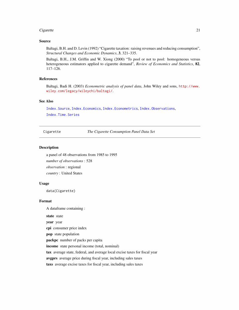
Cigarette The Cigarette Consumption Panel Data Set
Description
a panel of 48 observations from 1985 to 1995
number of observations : 528
observation : regional
country : United States
Usage
data(Cigarette)
Format
A dataframe containing :
state state
year year
cpi consumer price index
pop state population
packpc number of packs per capita
income state personal income (total, nominal)
tax average state, federal, and average local excise taxes for fiscal year
avgprs average price during fiscal year, including sales taxes
taxs average excise taxes for fiscal year, including sales taxes
22 Clothing
Source
Professor Jonathan Gruber, MIT.
References
Stock, James H. and Mark W. Watson (2003) Introduction to Econometrics, Addison-Wesley Edu-cational Publishers, chapter 10.
See Also
Index.Source, Index.Economics, Index.Econometrics, Index.Observations,
Index.Time.Series
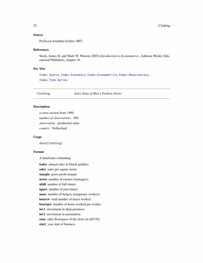
Clothing Sales Data of Men’s Fashion Stores
Description
a cross-section from 1990
number of observations : 400
observation : production units
country : Netherland
Usage
data(Clothing)
Format
A dataframe containing :
tsales annual sales in Dutch guilders
sales sales per square meter
margin gross-profit-margin
nown number of owners (managers)
nfull number of full-timers
npart number of part-timers
naux number of helpers (temporary workers)
hoursw total number of hours worked
hourspw number of hours worked per worker
inv1 investment in shop-premises
inv2 investment in automation.
ssize sales floorspace of the store (in m$^2$).
start year start of business
Computers 23
References
Verbeek, Marno (2004) A Guide to Modern Econometrics, John Wiley and Sons, chapter 3.
See Also
Index.Source, Index.Economics, Index.Econometrics, Index.Observations
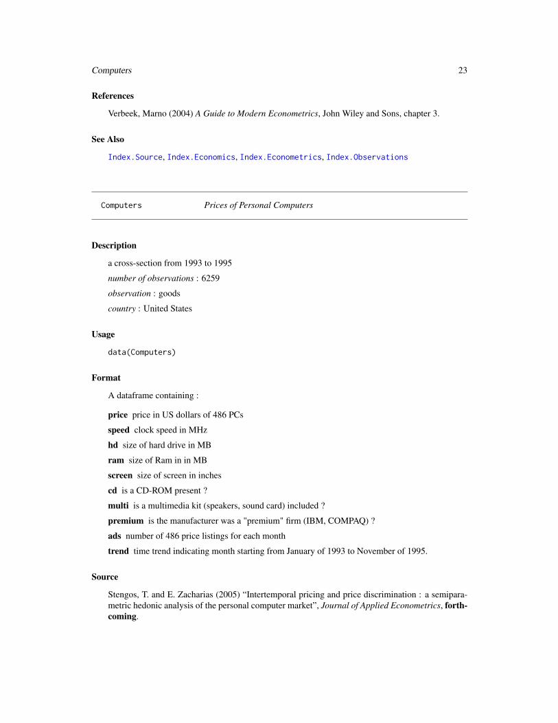
Computers Prices of Personal Computers
Description
a cross-section from 1993 to 1995
number of observations : 6259
observation : goods
country : United States
Usage
data(Computers)
Format
A dataframe containing :
price price in US dollars of 486 PCs
speed clock speed in MHz
hd size of hard drive in MB
ram size of Ram in in MB
screen size of screen in inches
cd is a CD-ROM present ?
multi is a multimedia kit (speakers, sound card) included ?
premium is the manufacturer was a "premium" firm (IBM, COMPAQ) ?
ads number of 486 price listings for each month
trend time trend indicating month starting from January of 1993 to November of 1995.
Source
Stengos, T. and E. Zacharias (2005) “Intertemporal pricing and price discrimination : a semipara-metric hedonic analysis of the personal computer market”, Journal of Applied Econometrics, forth-coming.

24 Consumption
References
Journal of Applied Econometrics data archive : http://qed.econ.queensu.ca/jae/.
See Also
Index.Source, Index.Economics, Index.Econometrics, Index.Observations
Consumption Quarterly Data on Consumption and Expenditure
Description
quarterly observations from 1947-1 to 1996-4
number of observations : 200
observation : country
country : Canada
Usage
data(Consumption)
Format
A time serie containing :
yd personal disposable income, 1986 dollars
ce personal consumption expenditure, 1986 dollars
References
Davidson, R. and James G. MacKinnon (2004) Econometric Theory and Methods, New York, Ox-ford University Press, http://www.econ.queensu.ca/ETM/, chapter 1, 3, 4, 6, 9, 10, 14 and 15.
See Also
Index.Source, Index.Economics, Index.Econometrics, Index.Observations,
Index.Time.Series

CPSch3 25
CPSch3 Earnings from the Current Population Survey
Description
a cross-section from 1998
number of observations : 11130
observation : individuals
country : United States
Usage
data(CPSch3)
Format
A dataframe containing :
year survey year
ahe average hourly earnings
sex a factor with levels (male,female)
Source
Bureau of labor statistics, U.S. Department of Labor http://www.bls.gov.
References
Stock, James H. and Mark W. Watson (2003) Introduction to Econometrics, Addison-Wesley Edu-cational Publishers, chapter 3.
See Also
Index.Source, Index.Economics, Index.Econometrics, Index.Observations
26 Cracker
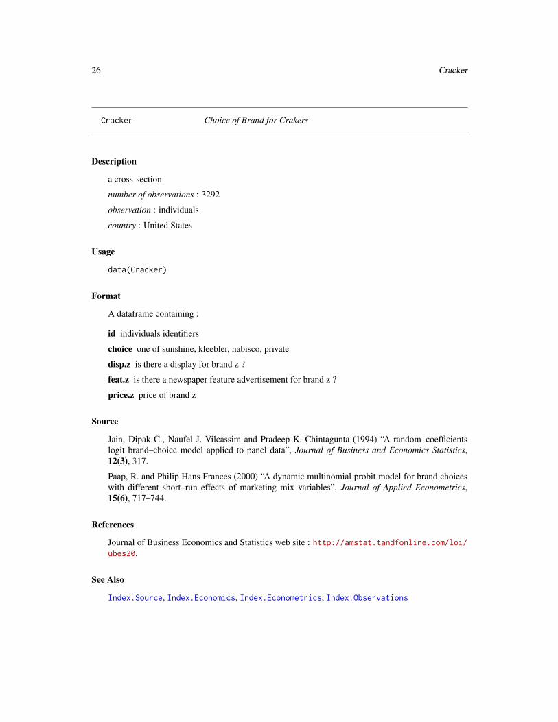
Cracker Choice of Brand for Crakers
Description
a cross-section
number of observations : 3292
observation : individuals
country : United States
Usage
data(Cracker)
Format
A dataframe containing :
id individuals identifiers
choice one of sunshine, kleebler, nabisco, private
disp.z is there a display for brand z ?
feat.z is there a newspaper feature advertisement for brand z ?
price.z price of brand z
Source
Jain, Dipak C., Naufel J. Vilcassim and Pradeep K. Chintagunta (1994) “A random–coefficientslogit brand–choice model applied to panel data”, Journal of Business and Economics Statistics,12(3), 317.
Paap, R. and Philip Hans Frances (2000) “A dynamic multinomial probit model for brand choiceswith different short–run effects of marketing mix variables”, Journal of Applied Econometrics,15(6), 717–744.
References
Journal of Business Economics and Statistics web site : http://amstat.tandfonline.com/loi/ubes20.
See Also
Index.Source, Index.Economics, Index.Econometrics, Index.Observations
CRANpackages 27
CRANpackages Growth of CRAN
Description
Data casually collected on the number of packages on the Comprehensive R Archive Network(CRAN) at different dates.
NOTE: This could change in the future. See Details below.
Usage
data(CRANpackages)
Format
A data.frame containing:
Version an ordered factor of the R version number primarily in use at the time. This was taken fromarchives of the major releases at https://svn.r-project.org/R/branches/R-1-3-patches/tests/internet.Rout.save, ... https://svn.r-project.org/R/branches/R-3-1-branch/tests/internet.Rout.save
Date an object of class Date giving the date on which the count of the number of CRAN packageswas determined.
Packages an integer number of packages on the CRAN mirror checked on the indicated Date.
Source A factor giving the source (person) who collected the data.
Details
This seems to provide the most widely available source for data on the growth of CRAN, manuallyrecorded by John Fox and Spencer Graves. For a discussion of these and related data, see Fox(2009).
For more detail, see the CRAN packages data on Github maintained by Hadley Wickham. Thiscontains the description file of every package uploaded to CRAN prior to the date of Hadley’smost recent update. The current maintainer of the Ecdat and Ecfun packages would considercontributions along the following lines:
1. It might be nice to have a more complete dataset or datasets showing CRAN growth. This mightinclude code fitting multiple models and predicting future growth with error bounds computed usingBayesian Model Averaging. These model fits might make an interesting addition to the examples inthis help file. With a little more effort, it might make an interesting note for R Journal. Functionswritten to fit those models might be added to the Ecfun package.
2. It might be nice to have a function in Ecfun to download the CRAN packages data from Githuband convert it to a format suitable for updating this dataset.
The current maintainer for Ecdat and Ecfun (Spencer Graves) might be willing to accept code anddocumentation for this but is not ready to do it himself at the present time.
28 Crime
Source
John Fox, "Aspects of the Social Organization and Trajectory of the R Project", R Journal, 1(2),Dec. 2009, 5-13. https://journal.r-project.org/archive/2009-2/RJournal_2009-2_Fox.pdf, accessed 2014-04-13.
Examples
plot(Packages~Date, CRANpackages, log='y')# almost exponential growth
Crime Crime in North Carolina
Description
a panel of 90 observations from 1981 to 1987
number of observations : 630
observation : regional
country : United States
Usage
data(Crime)
Format
A dataframe containing :
county county identifier
year year from 1981 to 1987
crmrte crimes committed per person
prbarr ’probability’ of arrest
prbconv ’probability’ of conviction
prbpris ’probability’ of prison sentence
avgsen average sentence, days
polpc police per capita
density people per square mile
taxpc tax revenue per capita
region one of ’other’, ’west’ or ’central’
smsa ’yes’ or ’no’ if in SMSA
pctmin percentage minority in 1980
wcon weekly wage in construction
CRSPday 29
wtuc weekly wage in trns, util, commun
wtrd weekly wage in whole sales and retail trade
wfir weekly wage in finance, insurance and real estate
wser weekly wage in service industry
wmfg weekly wage in manufacturing
wfed weekly wage of federal employees
wsta weekly wage of state employees
wloc weekly wage of local governments employees
mix offence mix: face-to-face/other
pctymle percentage of young males
Source
Cornwell, C. and W.N. Trumbull (1994) “Estimating the economic model of crime with panel data”,Review of Economics and Statistics, 76, 360–366.
Baltagi, B. H. (forthcoming) “Estimating an economic model of crime using panel data from NorthCarolina”, Journal of Applied Econometrics, .
References
Baltagi, Badi H. (2003) Econometric analysis of panel data, John Wiley and sons, http://www.wiley.com/legacy/wileychi/baltagi/, .
Journal of Applied Econometrics data archive : http://qed.econ.queensu.ca/jae/.
See Also
Index.Source, Index.Economics, Index.Econometrics, Index.Observations,
Index.Time.Series
CRSPday Daily Returns from the CRSP Database
Description
daily observations from 1969-1-03 to 1998-12-31
number of observations : 2528
observation : production units
country : United States
Usage
data(CRSPday)
30 CRSPmon
Format
A dataframe containing :
year the year
month the month
day the day
ge the return for General Electric, Permno 12060
ibm the return for IBM, Permno 12490
mobil the return for Mobil Corporation, Permno 15966
crsp the return for the CRSP value-weighted index, including dividends
Source
Center for Research in Security Prices, Graduate School of Business, University of Chicago, 725South Wells - Suite 800, Chicago, Illinois 60607, http://www.crsp.com.
References
Davidson, R. and James G. MacKinnon (2004) Econometric Theory and Methods, New York, Ox-ford University Press, http://www.econ.queensu.ca/ETM/, chapter 7, 9 and 15.
See Also
Index.Source, Index.Economics, Index.Econometrics, Index.Observations,
Index.Time.Series
CRSPmon Monthly Returns from the CRSP Database
Description
monthly observations from 1969-1 to 1998-12
number of observations : 360
observation : production units
country : United States
Usage
data(CRSPmon)
Diamond 31
Format
A time serie containing :
ge the return for General Electric, Permno 12060ibm the return for IBM, Permno 12490mobil the return for Mobil Corporation, Permno 15966crsp the return for the CRSP value-weighted index, including dividends
Source
Center for Research in Security Prices, Graduate School of Business, University of Chicago, 725South Wells - Suite 800, Chicago, Illinois 60607, http://www.crsp.com.
References
Davidson, R. and James G. MacKinnon (2004) Econometric Theory and Methods, New York, Ox-ford University Press, http://www.econ.queensu.ca/ETM/, chapter 13.
See Also
Index.Source, Index.Economics, Index.Econometrics, Index.Observations,
Index.Time.Series
Diamond Pricing the C’s of Diamond Stones
Description
a cross-section from 2000
number of observations : 308
observation : goods
country : Singapore
Usage
data(Diamond)
Format
A dataframe containing :
carat weight of diamond stones in carat unitcolour a factor with levels (D,E,F,G,H,I)clarity a factor with levels (IF,VVS1,VVS2,VS1,VS2)certification certification body, a factor with levels (GIA,IGI,HRD)price price in Singapore \$
32 DM
Source
Chu, Singfat (2001) “Pricing the C’s of Diamond Stones”, Journal of Statistics Education, 9(2).
References
Journal of Statistics Education’s data archive : http://www.amstat.org/publications/jse/jse_data_archive.htm.
See Also
Index.Source, Index.Economics, Index.Econometrics, Index.Observations
DM DM Dollar Exchange Rate
Description
weekly observations from 1975 to 1989
number of observations : 778
observation : country
country : Germany
Usage
data(DM)
Format
A dataframe containing :
date the date of the observation (19850104 is January, 4, 1985)
s the ask price of the dollar in units of DM in the spot market on friday of the current week
f the ask price of the dollar in units of DM in the 30-day forward market on friday of the currentweek
s30 the bid price of the dollar in units of DM in the spot market on the delivery date on a currentforward contract
Source
Bekaert, G. and R. Hodrick (1993) “On biases in the measurement of foreign exchange risk premi-ums”, Journal of International Money and Finance, 12, 115-138.
References
Hayashi, F. (2000) Econometrics, Princeton University Press, http://fhayashi.fc2web.com/hayashi_econometrics.htm, chapter 6, 438-443.
Doctor 33
See Also
Index.Source, Index.Economics, Index.Econometrics, Index.Observations,
Index.Time.Series
Doctor Number of Doctor Visits
Description
a cross-section from 1986
number of observations : 485
observation : individuals
country : United States
Usage
data(Doctor)
Format
A dataframe containing :
doctor the number of doctor visits
children the number of children in the household
access is a measure of access to health care
health a measure of health status (larger positive numbers are associated with poorer health)
Source
Gurmu, Shiferaw (1997) “Semiparametric estimation of hurdle regression models with an applica-tion to medicaid utilization”, Journal of Applied Econometrics, 12(3), 225-242.
References
Davidson, R. and James G. MacKinnon (2004) Econometric Theory and Methods, New York, Ox-ford University Press, http://www.econ.queensu.ca/ETM/, chapter 11.
Journal of Applied Econometrics data archive : http://qed.econ.queensu.ca/jae/.
See Also
Index.Source, Index.Economics, Index.Econometrics, Index.Observations

34 DoctorAUS
DoctorAUS Doctor Visits in Australia
Description
a cross-section from 1977–1978
number of observations : 5190
observation : individuals
country : Australia
Usage
data(DoctorAUS)
Format
A dataframe containing :
sex sex
age age
income annual income in tens of thousands of dollars
insurance insurance contract (medlevy : medibanl levy, levyplus : private health insurance, freep-oor : government insurance due to low income, freerepa : government insurance due to oldage disability or veteran status
illness number of illness in past 2 weeks
actdays number of days of reduced activity in past 2 weeks due to illness or injury
hscore general health score using Goldberg’s method (from 0 to 12)
chcond chronic condition (np : no problem, la : limiting activity, nla : not limiting activity)
doctorco number of consultations with a doctor or specialist in the past 2 weeks
nondocco number of consultations with non-doctor health professionals (chemist, optician, phys-iotherapist, social worker, district community nurse, chiropodist or chiropractor) in the past 2weeks
hospadmi number of admissions to a hospital, psychiatric hospital, nursing or convalescent homein the past 12 months (up to 5 or more admissions which is coded as 5)
hospdays number of nights in a hospital, etc. during most recent admission: taken, where appro-priate, as the mid-point of the intervals 1, 2, 3, 4, 5, 6, 7, 8-14, 15-30, 31-60, 61-79 with 80 ormore admissions coded as 80. If no admission in past 12 months then equals zero.
medecine total number of prescribed and nonprescribed medications used in past 2 days
prescrib total number of prescribed medications used in past 2 days
nonpresc total number of nonprescribed medications used in past 2 days
DoctorContacts 35
Source
Cameron, A.C. and P.K. Trivedi (1986) “Econometric Models Based on Count Data: Comparisonsand Applications of Some Estimators and Tests”, Journal of Applied Econometrics, 1, 29-54..
References
Cameron, A.C. and Trivedi P.K. (1998) Regression analysis of count data, Cambridge UniversityPress, http://cameron.econ.ucdavis.edu/racd/racddata.html, chapter 3.
See Also
Index.Source, Index.Economics, Index.Econometrics, Index.Observations
DoctorContacts Contacts With Medical Doctor
Description
a cross-section from 1977–1978
number of observations : 20186
Usage
data(DoctorContacts)
Format
A time serie containing :
mdu number of outpatient visits to a medical doctor
lc log(coinsrate+1) where coinsurance rate is 0 to 100
idp individual deductible plan ?
lpi log(annual participation incentive payment) or 0 if no payment
fmde log(max(medical deductible expenditure)) if IDP=1 and MDE>1 or 0 otherw
physlim physical limitation ?
ndisease number of chronic diseases
health self–rate health (excellent,good,fair,poor)
linc log of annual family income (in \$)
lfam log of family size
educdec years of schooling of household head
age exact age
sex sex (male,female)
child age less than 18 ?
black is household head black ?
36 Earnings
Source
Deb, P. and P.K. Trivedi (2002) “The Structure of Demand for Medical Care: Latent Class versusTwo-Part Models”, Journal of Health Economics, 21, 601–625.
References
Cameron, A.C. and P.K. Trivedi (2005) Microeconometrics : methods and applications, Cambridge,pp. 553–556 and 565.
See Also
Index.Source, Index.Economics, Index.Econometrics, Index.Observations,
Index.Time.Series
Earnings Earnings for Three Age Groups
Description
a cross-section from 1988-1989
number of observations : 4266
observation : individuals
country : United States
Usage
data(Earnings)
Format
A dataframe containing :
age age groups, a factor with levels (g1,g2,g3)
y average annual earnings, in 1982 US dollars
Source
Mills, Jeffery A. and Sourushe Zandvakili (1997) “Statistical Inference via Bootstrapping for Mea-sures of Inequality”, Journal of Applied Econometrics, 12(2), pp. 133-150.
References
Davidson, R. and James G. MacKinnon (2004) Econometric Theory and Methods, New York, Ox-ford University Press, http://www.econ.queensu.ca/ETM/, chapter 5 and 7.
Journal of Applied Econometrics data archive : http://qed.econ.queensu.ca/jae/.
Electricity 37
See Also
Index.Source, Index.Economics, Index.Econometrics, Index.Observations
Electricity Cost Function for Electricity Producers
Description
a cross-section from 1970 to 1970
number of observations : 158
observation : production units
country : United States
Usage
data(Electricity)
Format
A dataframe containing :
cost total costq total outputpl wage ratesl cost share for laborpk capital price indexsk cost share for capitalpf fuel pricesf cost share for fuel
Source
Christensen, L. and W. H. Greene (1976) “Economies of scale in U.S. electric power generation”,Journal of Political Economy, 84, 655-676.
References
Greene, W.H. (2003) Econometric Analysis, Prentice Hall, http://www.prenhall.com/greene/greene1.html, chapter 4, 317-320.
Hayashi, F. (2000) Econometrics, Princeton University Press, http://fhayashi.fc2web.com/hayashi_econometrics.htm, chapter 1, 76-84.
See Also
Index.Source, Index.Economics, Index.Econometrics, Index.Observations

38 Fair
Fair Extramarital Affairs Data
Description
a cross-section
number of observations : 601
observation : individuals
country : United States
Usage
data(Fair)
Format
A dataframe containing :
sex a factor with levels (male,female)
age age
ym number of years married
child children ? a factor
religious how religious, from 1 (anti) to 5 (very)
education education
occupation occupation, from 1 to 7, according to hollingshead classification (reverse numbering)
rate self rating of marriage, from 1 (very unhappy) to 5 (very happy)
nbaffairs number of affairs in past year
Source
Fair, R. (1977) “A note on the computation of the tobit estimator”, Econometrica, 45, 1723-1727.
http://fairmodel.econ.yale.edu/rayfair/pdf/1978A200.PDF.
References
Greene, W.H. (2003) Econometric Analysis, Prentice Hall, http://www.prenhall.com/greene/greene1.html, Table F22.2.
See Also
Index.Source, Index.Economics, Index.Econometrics, Index.Observations
Fatality 39
Fatality Drunk Driving Laws and Traffic Deaths
Description
a panel of 48 observations from 1982 to 1988
number of observations : 336
observation : regional
country : United States
Usage
data(Fatality)
Format
A dataframe containing :
state state ID code
year year
mrall traffic fatality rate (deaths per 10000)
beertax tax on case of beer
mlda minimum legal drinking age
jaild mandatory jail sentence ?
comserd mandatory community service ?
vmiles average miles per driver
unrate unemployment rate
perinc per capita personal income
Source
Pr. Christopher J. Ruhm, Department of Economics, University of North Carolina.
References
Stock, James H. and Mark W. Watson (2003) Introduction to Econometrics, Addison-Wesley Edu-cational Publishers, chapter 8.
See Also
Index.Source, Index.Economics, Index.Econometrics, Index.Observations,
Index.Time.Series
40 FinancialCrisisFiles
FinancialCrisisFiles Files containing financial crisis data
Description
FinancialCrisisFiles is an object of class financialCrisisFiles created by the financialCrisisFilesfunction in Ecfun. It describes files containing data on financial crises downloadable from http://www.reinhartandrogoff.com/data/browse-by-topic/topics/7/.
Usage
data(FinancialCrisisFiles)
Details
Reinhart and Rogoff (http://www.reinhartandrogoff.com) provide numerous data sets ana-lyzed in their book, "This Time Is Different: Eight Centuries of Financial Folly". Of interest hereare data on financial crises of various types for 70 countries spanning the years 1800 - 2010, down-loadable from http://www.reinhartandrogoff.com/data/browse-by-topic/topics/7/.
The function financialCrisisFiles in Ecfun produces a list of class financialCrisisFilesdescribing four different Excel files in very similar formats with one sheet per Country and a fewextra descriptor sheets. The data object FinancialCrisisFiles is the default output of that func-tion.
Value
FinancialCrisisFiles is a list with components carrying the names of files to be read. Eachcomponent is a list of optional arguments to pass to do.call(read.xls, ...) to read the sheetwith name = name of that component.
This corresponds to the files downloaded from http://www.reinhartandrogoff.com/data/browse-by-topic/topics/7/ in January 2013 (except for the fourth, which was not available there because of an errorwith the web site but instead was obtained directly from Prof. Reinhart).
Author(s)
Spencer Graves
Source
http://www.reinhartandrogoff.com
References
Carmen M. Reinhart and Kenneth S. Rogoff (2009) This Time Is Different: Eight Centuries ofFinancial Folly, Princeton U. Pr.
Fishing 41
See Also
read.xls
Fishing Choice of Fishing Mode
Description
a cross-section
number of observations : 1182
observation : individuals
country : United States
Usage
data(Fishing)
Format
A dataframe containing :
mode recreation mode choice, on of : beach, pier, boat and charter
price price for chosen alternative
catch catch rate for chosen alternative
pbeach price for beach mode
ppier price for pier mode
pboat price for private boat mode
pcharter price for charter boat mode
cbeach catch rate for beach mode
cpier catch rate for pier mode
cboat catch rate for private boat mode
ccharter catch rate for charter boat mode
income monthly income
Source
Herriges, J. A. and C. L. Kling (1999) “Nonlinear Income Effects in Random Utility Models”,Review of Economics and Statistics, 81, 62-72.
References
Cameron, A.C. and P.K. Trivedi (2005) Microeconometrics : methods and applications, Cambridge,pp. 463–466, 486 and 491–495.

42 Forward
See Also
Index.Source, Index.Economics, Index.Econometrics, Index.Observations
Forward Exchange Rates of US Dollar Against Other Currencies
Description
monthly observations from 1979–01 to 2001–12
number of observations : 276
Usage
data(Forward)
Format
A time serie containing :
usdbp exchange rate USD/British Pound Sterling
usdeuro exchange rate US D/Euro
eurobp exchange rate Euro/Pound
usdbp1 1 month forward rate USD/Pound
usdeuro1 1 month forward rate USD/Euro
eurobp1 1 month forward rate Euro/Pound
usdbp3 3 month forward rate USD/Pound
usdeuro3 month forward rate USD/Euro
eurobp3 month forward rate Euro/Pound
Source
Datastream .
References
Verbeek, Marno (2004) A Guide to Modern Econometrics, John Wiley and Sons, chapter 4.
See Also
Index.Source, Index.Economics, Index.Econometrics, Index.Observations,
Index.Time.Series
FriendFoe 43
FriendFoe Data from the Television Game Show Friend Or Foe ?
Description
a cross-section from 2002–03
number of observations : 227
observation : individuals
country : United States
Usage
data(FriendFoe)
Format
A dataframe containing :
sex contestant’s sex
white is contestant white ?
age contestant’s age in years
play contestant’s choice : a factor with levels "foe" and "friend". If both players play "friend",they share the trust box, if both play "foe", both players receive zero prize, if one of them play"foe" and the other one "friend", the "foe" player receive the entire trust bix and the "friend"player nothing
round round in which contestant is eliminated, a factor with levels ("1","2","3")
season season show, a factor with levels ("1","2")
cash the amount of cash in the trust box
sex1 partner’s sex
white1 is partner white ?
age1 partner’s age in years
play1 partner’s choice : a factor with levels "foe" and "friend"
win money won by contestant
win1 money won by partner
Source
Kalist, David E. (2004) “Data from the Television Game Show "Friend or Foe?"”, Journal of Statis-tics Education, 12(3).
References
Journal of Statistics Education’s data archive : http://www.amstat.org/publications/jse/jse_data_archive.htm.
44 Garch
See Also
Index.Source, Index.Economics, Index.Econometrics, Index.Observations
Garch Daily Observations on Exchange Rates of the US Dollar Against OtherCurrencies
Description
daily observations from 1980–01 to 1987–05–21
number of observations : 1867
observation : country
country : World
Usage
data(Garch)
Format
A dataframe containing :
date date of observation (yymmdd)
day day of the week (a factor)
dm exchange rate Dollar/Deutsch Mark
ddm dm-dm(-1)
bp exchange rate of Dollar/British Pound
cd exchange rate of Dollar/Canadian Dollar
dy exchange rate of Dollar/Yen
sf exchange rate of Dollar/Swiss Franc
References
Verbeek, Marno (2004) A Guide to Modern Econometrics, John Wiley and Sons, chapter 8.
See Also
Index.Source, Index.Economics, Index.Econometrics, Index.Observations,
Index.Time.Series
Gasoline 45
Gasoline Gasoline Consumption
Description
a panel of 18 observations from 1960 to 1978
number of observations : 342
observation : country
country : OECD
Usage
data(Gasoline)
Format
A dataframe containing :
country a factor with 18 levels
year the year
lgaspcar logarithm of motor gasoline consumption per auto
lincomep logarithm of real per-capita income
lrpmg logarithm of real motor gasoline price
lcarpcap logarithm of the stock of cars per capita
Source
Baltagi, B.H. and Y.J. Griggin (1983) “Gasoline demand in the OECD: an application of poolingand testing procedures”, European Economic Review, 22.
References
Baltagi, Badi H. (2003) Econometric analysis of panel data, John Wiley and sons, http://www.wiley.com/legacy/wileychi/baltagi/.
See Also
Index.Source, Index.Economics, Index.Econometrics, Index.Observations,
Index.Time.Series
46 Griliches
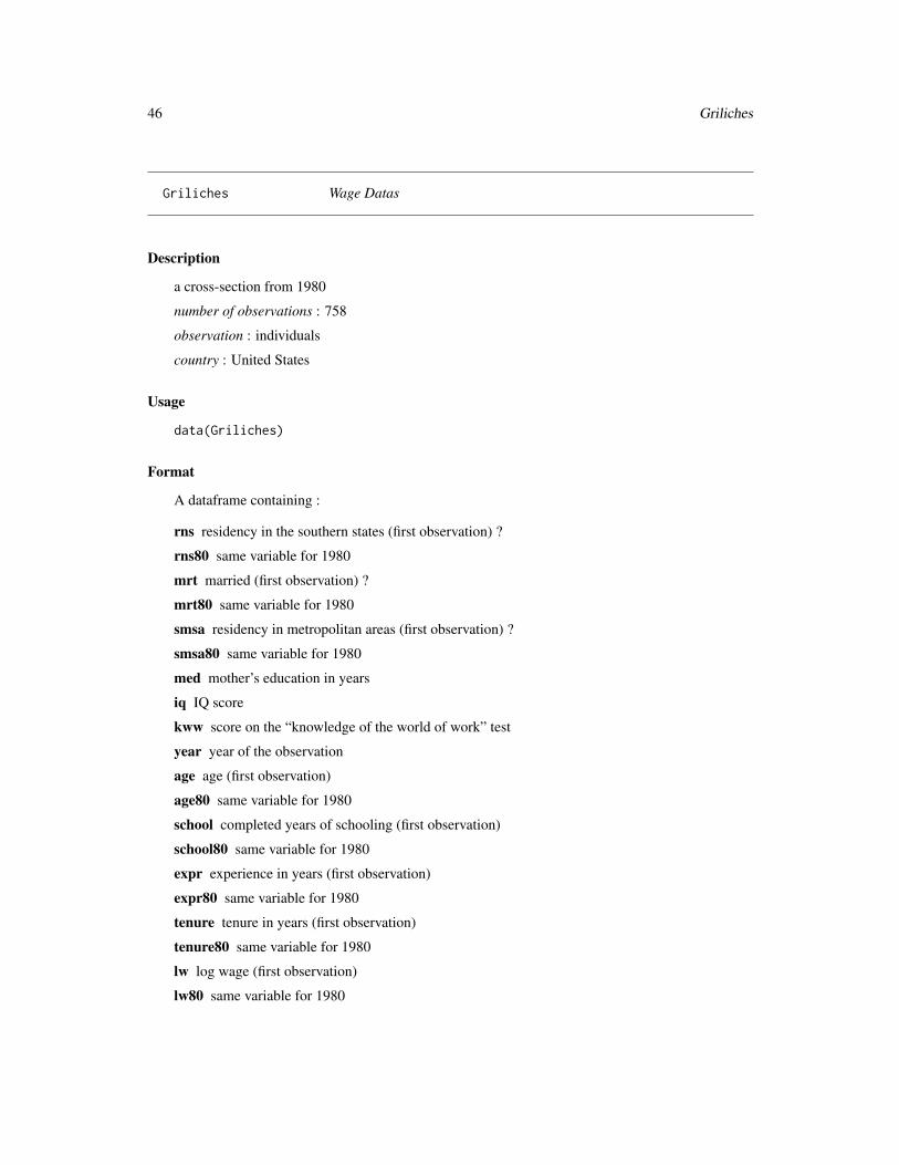
Griliches Wage Datas
Description
a cross-section from 1980
number of observations : 758
observation : individuals
country : United States
Usage
data(Griliches)
Format
A dataframe containing :
rns residency in the southern states (first observation) ?
rns80 same variable for 1980
mrt married (first observation) ?
mrt80 same variable for 1980
smsa residency in metropolitan areas (first observation) ?
smsa80 same variable for 1980
med mother’s education in years
iq IQ score
kww score on the “knowledge of the world of work” test
year year of the observation
age age (first observation)
age80 same variable for 1980
school completed years of schooling (first observation)
school80 same variable for 1980
expr experience in years (first observation)
expr80 same variable for 1980
tenure tenure in years (first observation)
tenure80 same variable for 1980
lw log wage (first observation)
lw80 same variable for 1980
Grunfeld 47
Source
Blackburn, M. and Neumark D. (1992) “Unobserved ability, efficiency wages, and interindustrywage differentials”, Quarterly Journal of Economics, 107, 1421-1436.
References
Hayashi, F. (2000) Econometrics, Princeton University Press, http://fhayashi.fc2web.com/hayashi_econometrics.htm, chapter 3, 250-256.
See Also
Index.Source, Index.Economics, Index.Econometrics, Index.Observations
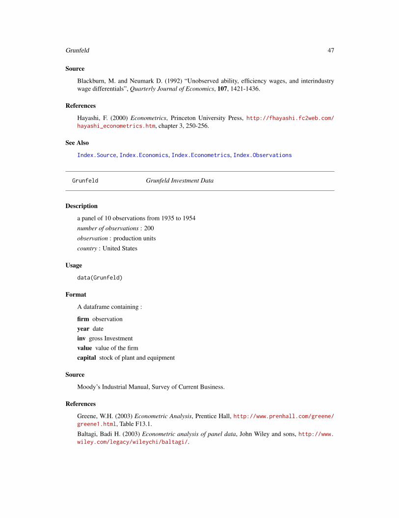
Grunfeld Grunfeld Investment Data
Description
a panel of 10 observations from 1935 to 1954
number of observations : 200
observation : production units
country : United States
Usage
data(Grunfeld)
Format
A dataframe containing :
firm observationyear dateinv gross Investmentvalue value of the firmcapital stock of plant and equipment
Source
Moody’s Industrial Manual, Survey of Current Business.
References
Greene, W.H. (2003) Econometric Analysis, Prentice Hall, http://www.prenhall.com/greene/greene1.html, Table F13.1.
Baltagi, Badi H. (2003) Econometric analysis of panel data, John Wiley and sons, http://www.wiley.com/legacy/wileychi/baltagi/.

48 HC
See Also
Index.Source, Index.Economics, Index.Econometrics, Index.Observations,
Index.Time.Series
HC Heating and Cooling System Choice in Newly Built Houses in Califor-nia
Description
a cross-section
number of observations : 250
observation : households
country : California
Usage
data(HC)
Format
A dataframe containing :
depvar heating system, one of gcc (gas central heat with cooling), ecc (electric central resistenceheat with cooling), erc (electric room resistence heat with cooling), hpc (electric heat pumpwhich provides cooling also), gc (gas central heat without cooling, ec (electric central re-sistence heat without cooling), er (electric room resistence heat without cooling)
ich.z installation cost of the heating portion of the system
icca installation cost for cooling
och.z operating cost for the heating portion of the system
occa operating cost for cooling
income annual income of the household
References
Kenneth Train’s home page : http://elsa.berkeley.edu/~train/.
See Also
Index.Source, Index.Economics, Index.Econometrics, Index.Observations

Heating 49
Heating Heating System Choice in California Houses
Description
a cross-section
number of observations : 900
observation : households
country : California
Usage
data(Heating)
Format
A dataframe containing :
idcase id
depvar heating system, one of gc (gas central), gr (gas room), ec (electric central), er (electricroom), hp (heat pump)
ic.z installation cost for heating system z (defined for the 5 heating systems)
oc.z annual operating cost for heating system z (defined for the 5 heating systems)
pb.z ratio oc.z/ic.z
income annual income of the household
agehed age of the household head
rooms numbers of rooms in the house
References
Kenneth Train’s home page : http://elsa.berkeley.edu/~train/.
See Also
Index.Source, Index.Economics, Index.Econometrics, Index.Observations

50 Hedonic
Hedonic Hedonic Prices of Census Tracts in Boston
Description
a cross-section
number of observations : 506
observation : regional
country : United States
Usage
data(Hedonic)
Format
A dataframe containing :
mv median value of owner–occupied homes
crim crime rate
zn proportion of 25,000 square feet residential lots
indus proportion of nonretail business acres
chas is the tract bounds the Charles River ?
nox annual average nitrogen oxide concentration in parts per hundred million
rm average number of rooms
age proportion of owner units built prior to 1940
dis weighted distances to five employment centers in the Boston area
rad index of accessibility to radial highways
tax full value property tax rate (\$/\$10,000)
ptratio pupil/teacher ratio
blacks proportion of blacks in the population
lstat proportion of population that is lower status
townid town identifier
Source
Harrison, D. and D.L. Rubinfeld (1978) “Hedonic housing prices and the demand for clean air”,Journal of Environmental Economics Ans Management, 5, 81–102.
Belsley, D.A., E. Kuh and R. E. Welsch (1980) Regression diagnostics: identifying influential dataand sources of collinearity, John Wiley, New–York.
HHSCyberSecurityBreaches 51
References
Baltagi, Badi H. (2003) Econometric analysis of panel data, John Wiley and sons, http://www.wiley.com/legacy/wileychi/baltagi/.
See Also
Index.Source, Index.Economics, Index.Econometrics, Index.Observations
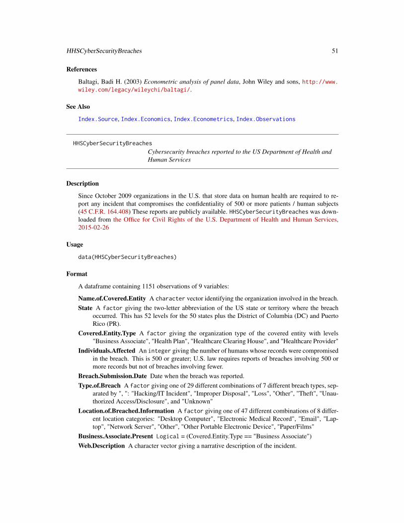
HHSCyberSecurityBreaches
Cybersecurity breaches reported to the US Department of Health andHuman Services
Description
Since October 2009 organizations in the U.S. that store data on human health are required to re-port any incident that compromises the confidentiality of 500 or more patients / human subjects(45 C.F.R. 164.408) These reports are publicly available. HHSCyberSecurityBreaches was down-loaded from the Office for Civil Rights of the U.S. Department of Health and Human Services,2015-02-26
Usage
data(HHSCyberSecurityBreaches)
Format
A dataframe containing 1151 observations of 9 variables:
Name.of.Covered.Entity A character vector identifying the organization involved in the breach.State A factor giving the two-letter abbreviation of the US state or territory where the breach
occurred. This has 52 levels for the 50 states plus the District of Columbia (DC) and PuertoRico (PR).
Covered.Entity.Type A factor giving the organization type of the covered entity with levels"Business Associate", "Health Plan", "Healthcare Clearing House", and "Healthcare Provider"
Individuals.Affected An integer giving the number of humans whose records were compromisedin the breach. This is 500 or greater; U.S. law requires reports of breaches involving 500 ormore records but not of breaches involving fewer.
Breach.Submission.Date Date when the breach was reported.Type.of.Breach A factor giving one of 29 different combinations of 7 different breach types, sep-
arated by ", ": "Hacking/IT Incident", "Improper Disposal", "Loss", "Other", "Theft", "Unau-thorized Access/Disclosure", and "Unknown"
Location.of.Breached.Information A factor giving one of 47 different combinations of 8 differ-ent location categories: "Desktop Computer", "Electronic Medical Record", "Email", "Lap-top", "Network Server", "Other", "Other Portable Electronic Device", "Paper/Films"
Business.Associate.Present Logical = (Covered.Entity.Type == "Business Associate")Web.Description A character vector giving a narrative description of the incident.
52 HHSCyberSecurityBreaches
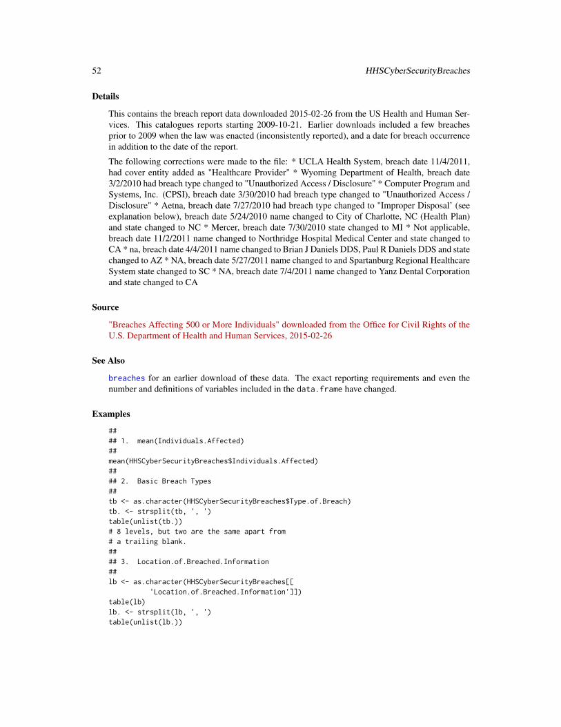
Details
This contains the breach report data downloaded 2015-02-26 from the US Health and Human Ser-vices. This catalogues reports starting 2009-10-21. Earlier downloads included a few breachesprior to 2009 when the law was enacted (inconsistently reported), and a date for breach occurrencein addition to the date of the report.
The following corrections were made to the file: * UCLA Health System, breach date 11/4/2011,had cover entity added as "Healthcare Provider" * Wyoming Department of Health, breach date3/2/2010 had breach type changed to "Unauthorized Access / Disclosure" * Computer Program andSystems, Inc. (CPSI), breach date 3/30/2010 had breach type changed to "Unauthorized Access /Disclosure" * Aetna, breach date 7/27/2010 had breach type changed to "Improper Disposal’ (seeexplanation below), breach date 5/24/2010 name changed to City of Charlotte, NC (Health Plan)and state changed to NC * Mercer, breach date 7/30/2010 state changed to MI * Not applicable,breach date 11/2/2011 name changed to Northridge Hospital Medical Center and state changed toCA * na, breach date 4/4/2011 name changed to Brian J Daniels DDS, Paul R Daniels DDS and statechanged to AZ * NA, breach date 5/27/2011 name changed to and Spartanburg Regional HealthcareSystem state changed to SC * NA, breach date 7/4/2011 name changed to Yanz Dental Corporationand state changed to CA
Source
"Breaches Affecting 500 or More Individuals" downloaded from the Office for Civil Rights of theU.S. Department of Health and Human Services, 2015-02-26
See Also
breaches for an earlier download of these data. The exact reporting requirements and even thenumber and definitions of variables included in the data.frame have changed.
Examples
#### 1. mean(Individuals.Affected)##mean(HHSCyberSecurityBreaches$Individuals.Affected)#### 2. Basic Breach Types##tb <- as.character(HHSCyberSecurityBreaches$Type.of.Breach)tb. <- strsplit(tb, ', ')table(unlist(tb.))# 8 levels, but two are the same apart from# a trailing blank.#### 3. Location.of.Breached.Information##lb <- as.character(HHSCyberSecurityBreaches[[
'Location.of.Breached.Information']])table(lb)lb. <- strsplit(lb, ', ')table(unlist(lb.))
HI 53
# 8 levelstable(sapply(lb., length))# 1 2 3 4 5 6 7 8#1007 119 13 8 1 1 1 1# all 8 levels together observed once# There are 256 = 2^8 possible combinations# of which 47 actually occur in these data.
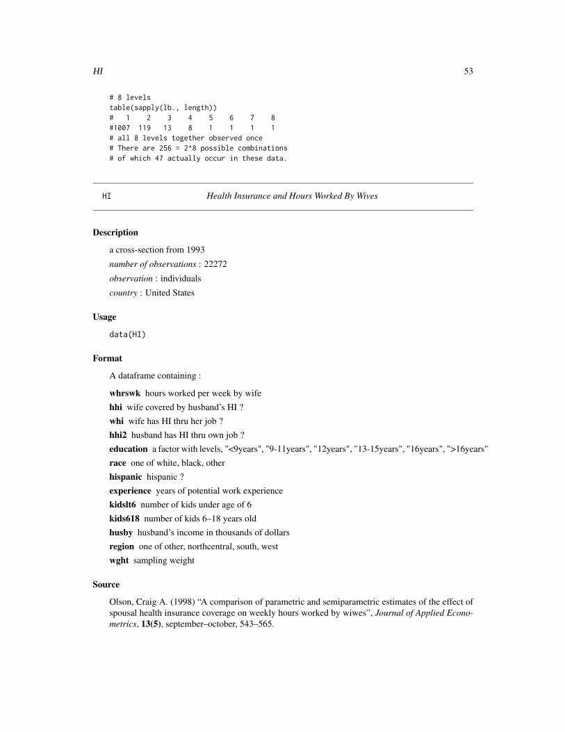
HI Health Insurance and Hours Worked By Wives
Description
a cross-section from 1993
number of observations : 22272
observation : individuals
country : United States
Usage
data(HI)
Format
A dataframe containing :
whrswk hours worked per week by wife
hhi wife covered by husband’s HI ?
whi wife has HI thru her job ?
hhi2 husband has HI thru own job ?
education a factor with levels, "<9years", "9-11years", "12years", "13-15years", "16years", ">16years"
race one of white, black, other
hispanic hispanic ?
experience years of potential work experience
kidslt6 number of kids under age of 6
kids618 number of kids 6–18 years old
husby husband’s income in thousands of dollars
region one of other, northcentral, south, west
wght sampling weight
Source
Olson, Craig A. (1998) “A comparison of parametric and semiparametric estimates of the effect ofspousal health insurance coverage on weekly hours worked by wiwes”, Journal of Applied Econo-metrics, 13(5), september–october, 543–565.

54 Hmda
References
Journal of Applied Econometrics data archive : http://qed.econ.queensu.ca/jae/.
See Also
Index.Source, Index.Economics, Index.Econometrics, Index.Observations
Hmda The Boston HMDA Data Set
Description
a cross-section from 1997-1998
number of observations : 2381 observation : individuals country : United States
In package version 0.2-9 and earlier this dataset was called Hdma.
Usage
data(Hmda)
Format
A dataframe containing :
dir debt payments to total income ratio
hir housing expenses to income ratio
lvr ratio of size of loan to assessed value of property
ccs consumer credit score from 1 to 6 (a low value being a good score)
mcs mortgage credit score from 1 to 4 (a low value being a good score)
pbcr public bad credit record ?
dmi denied mortgage insurance ?
self self employed ?
single is the applicant single ?
uria 1989 Massachusetts unemployment rate in the applicant’s industry
condominium is unit a condominium ? (was called comdominiom in version 0.2-9 and earlierversions of the package)
black is the applicant black ?
deny mortgage application denied ?
Source
Federal Reserve Bank of Boston.
Munnell, Alicia H., Geoffrey M.B. Tootell, Lynne E. Browne and James McEneaney (1996) “Mort-gage lending in Boston: Interpreting HMDA data”, American Economic Review, 25-53.
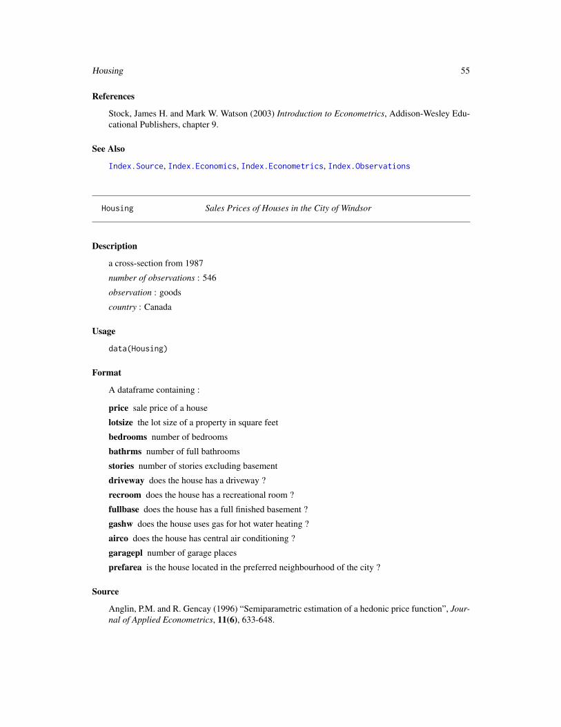
Housing 55
References
Stock, James H. and Mark W. Watson (2003) Introduction to Econometrics, Addison-Wesley Edu-cational Publishers, chapter 9.
See Also
Index.Source, Index.Economics, Index.Econometrics, Index.Observations
Housing Sales Prices of Houses in the City of Windsor
Description
a cross-section from 1987
number of observations : 546
observation : goods
country : Canada
Usage
data(Housing)
Format
A dataframe containing :
price sale price of a house
lotsize the lot size of a property in square feet
bedrooms number of bedrooms
bathrms number of full bathrooms
stories number of stories excluding basement
driveway does the house has a driveway ?
recroom does the house has a recreational room ?
fullbase does the house has a full finished basement ?
gashw does the house uses gas for hot water heating ?
airco does the house has central air conditioning ?
garagepl number of garage places
prefarea is the house located in the preferred neighbourhood of the city ?
Source
Anglin, P.M. and R. Gencay (1996) “Semiparametric estimation of a hedonic price function”, Jour-nal of Applied Econometrics, 11(6), 633-648.

56 Hstarts
References
Verbeek, Marno (2004) A Guide to Modern Econometrics, John Wiley and Sons, chapter 3.
Journal of Applied Econometrics data archive : http://qed.econ.queensu.ca/jae/.
See Also
Index.Source, Index.Economics, Index.Econometrics, Index.Observations
Hstarts Housing Starts
Description
quarterly observations from 1960-1 to 2001-4
number of observations : 168
observation : country
country : Canada
Usage
data(Hstarts)
Format
A time serie containing :
hs the log of urban housing starts in Canada, not seasonally adjusted, CANSIM series J6001, con-verted to quarterly
hssa the log of urban housing starts in Canada, seasonally adjusted, CANSIM series J9001, con-verted to quarterly. Observations prior to 1966:1 are missing
References
Davidson, R. and James G. MacKinnon (2004) Econometric Theory and Methods, New York, Ox-ford University Press, http://www.econ.queensu.ca/ETM/, chapter 13.
See Also
Index.Source, Index.Economics, Index.Econometrics, Index.Observations,
Index.Time.Series
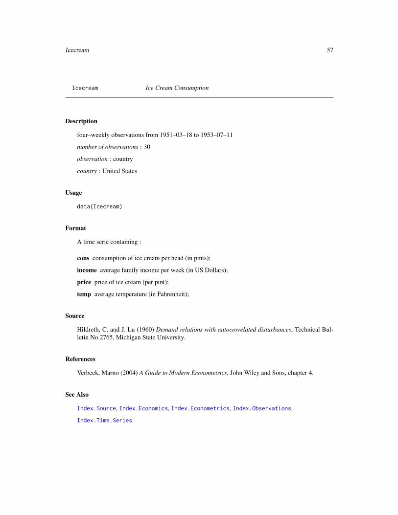
Icecream 57
Icecream Ice Cream Consumption
Description
four–weekly observations from 1951–03–18 to 1953–07–11
number of observations : 30
observation : country
country : United States
Usage
data(Icecream)
Format
A time serie containing :
cons consumption of ice cream per head (in pints);
income average family income per week (in US Dollars);
price price of ice cream (per pint);
temp average temperature (in Fahrenheit);
Source
Hildreth, C. and J. Lu (1960) Demand relations with autocorrelated disturbances, Technical Bul-letin No 2765, Michigan State University.
References
Verbeek, Marno (2004) A Guide to Modern Econometrics, John Wiley and Sons, chapter 4.
See Also
Index.Source, Index.Economics, Index.Econometrics, Index.Observations,
Index.Time.Series
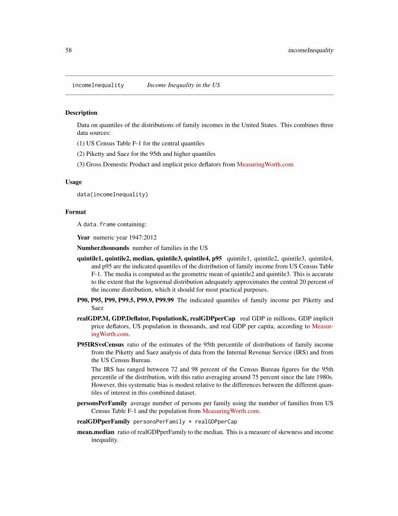
58 incomeInequality
incomeInequality Income Inequality in the US
Description
Data on quantiles of the distributions of family incomes in the United States. This combines threedata sources:
(1) US Census Table F-1 for the central quantiles
(2) Piketty and Saez for the 95th and higher quantiles
(3) Gross Domestic Product and implicit price deflators from MeasuringWorth.com
Usage
data(incomeInequality)
Format
A data.frame containing:
Year numeric year 1947:2012
Number.thousands number of families in the US
quintile1, quintile2, median, quintile3, quintile4, p95 quintile1, quintile2, quintile3, quintile4,and p95 are the indicated quantiles of the distribution of family income from US Census TableF-1. The media is computed as the geometric mean of quintile2 and quintile3. This is accurateto the extent that the lognormal distribution adequately approximates the central 20 percent ofthe income distribution, which it should for most practical purposes.
P90, P95, P99, P99.5, P99.9, P99.99 The indicated quantiles of family income per Piketty andSaez
realGDP.M, GDP.Deflator, PopulationK, realGDPperCap real GDP in millions, GDP implicitprice deflators, US population in thousands, and real GDP per capita, according to Measur-ingWorth.com.
P95IRSvsCensus ratio of the estimates of the 95th percentile of distributions of family incomefrom the Piketty and Saez analysis of data from the Internal Revenue Service (IRS) and fromthe US Census Bureau.The IRS has ranged between 72 and 98 percent of the Census Bureau figures for the 95thpercentile of the distribution, with this ratio averaging around 75 percent since the late 1980s.However, this systematic bias is modest relative to the differences between the different quan-tiles of interest in this combined dataset.
personsPerFamily average number of persons per family using the number of families from USCensus Table F-1 and the population from MeasuringWorth.com.
realGDPperFamily personsPerFamily * realGDPperCap
mean.median ratio of realGDPperFamily to the median. This is a measure of skewness and incomeinequality.

incomeInequality 59
Details
For details on how this data.frame was created, see "F1.PikettySaez.R" in system.file('scripts', package='fda').This provides links for files to download and R commands to read those files and convert them intoan updated version of incomeInequality. This is a reasonable thing to do if it is more than 2 yearssince max(incomeInequality$year). All data are in constant 2012 dollars.
Author(s)
Spencer Graves
Source
United States Census Bureau, Table F-1. Income Limits for Each Fifth and Top 5 Percent of Fami-lies, All Races, http://www.census.gov/data/tables/time-series/demo/income-poverty/historical-income-inequality.html, accessed 2016-12-09.
Thomas Piketty and Emmanuel Saez (2003) "Income Inequality in the United States, 1913-1998",Quarterly Journal of Economics, 118(1) 1-39, http://elsa.berkeley.edu/~saez, update ac-cessed February 28, 2014.
Louis Johnston and Samuel H. Williamson (2011) "What Was the U.S. GDP Then?" Measuring-Worth, http://www.measuringworth.org/usgdp, accessed February 28, 2014.
Examples
#### Rato of IRS to census estimates for the 95th percentile##data(incomeInequality)plot(P95IRSvsCensus~Year, incomeInequality, type='b')# starts ~0.74, trends rapidly up to ~0.97,# then drifts back to ~0.75abline(h=0.75)abline(v=1989)# checksum(is.na(incomeInequality$P95IRSvsCensus))# The Census data runs to 2011; Pikety and Saez runs to 2010.quantile(incomeInequality$P95IRSvsCensus, na.rm=TRUE)# 0.72 ... 0.98
#### Persons per Family##
plot(personsPerFamily~Year, incomeInequality, type='b')quantile(incomeInequality$personsPerFamily)# ranges from 3.72 to 4.01 with median 3.84# -- almost 4
#### GDP per family##
60 incomeInequality
plot(realGDPperFamily~Year, incomeInequality, type='b', log='y')
#### Plot the mean then the first quintile, then the median,## 99th, 99.9th and 99.99th percentiles##plotCols <- c(21, 3, 5, 11, 13:14)kcols <- length(plotCols)plotColors <- c(1:6, 8:13)[1:kcols] # omit 7=yellowplotLty <- 1:kcols
matplot(incomeInequality$Year, incomeInequality[plotCols]/1000,log='y', type='l', col=plotColors, lty=plotLty)
#*** Growth broadly shared 1947 - 1970, then began diverging#*** The divergence has been most pronounced among the top 1%#*** and especially the top 0.01%
#### Growth rate by quantile 1947-1970 and 1970 - present##keyYears <- c(1947, 1970, 2010)(iYears <- which(is.element(incomeInequality$Year, keyYears)))
(dYears <- diff(keyYears))kk <- length(keyYears)(lblYrs <- paste(keyYears[-kk], keyYears[-1], sep='-'))
(growth <- sapply(incomeInequality[iYears,], function(x, labels=lblYrs){dxi <- exp(diff(log(x)))names(dxi) <- labelsdxi
} ))
# as percent(gr <- round(100*(growth-1), 1))
# The average annual income (realGDPperFamily) doubled between# 1970 and 2010 (increased by 101 percent), while the median household# income increased only 23 percent.
#### Income lost by each quantile 1970-2010## relative to the broadly shared growth 1947-1970##(lostGrowth <- (growth[, 'realGDPperFamily']-growth[, plotCols]))# 1947-1970: The median gained 20% relative to the mean,# while the top 1% lost ground# 1970-2010: The median lost 79%, the 99th percentile lost 29%,# while the top 0.1% gained
(lostIncome <- (lostGrowth[2, ] *incomeInequality[iYears[2], plotCols]))
incomeInequality 61
# The median family lost $39,000 per year in income# relative to what they would have with the same economic growth# broadly shared as during 1947-1970.# That's slightly over $36,500 per year = $100 per day
(grYr <- growth^(1/dYears))(grYr. <- round(100*(grYr-1), 1))
#### Regression line: linear spline##
(varyg <- c(3:14, 21))Varyg <- names(incomeInequality)[varyg]str(F01ps <- reshape(incomeInequality[c(1, varyg)], idvar='Year',
ids=F1.PikettySeaz$Year,times=Varyg, timevar='pctile',varying=list(Varyg), direction='long'))
names(F01ps)[2:3] <- c('variable', 'value')F01ps$variable <- factor(F01ps$variable)
# linear spline basis function with knot at 1970F01ps$t1970p <- pmax(0, F01ps$Year-1970)
table(nas <- is.na(F01ps$value))# 6 NAs, one each of the Piketty-Saez variables in 2011F01i <- F01ps[!nas, ]
# formula:# log(value/1000) ~ b*Year + (for each variable:# different intercept + (different slope after 1970))
Fit <- lm(log(value/1000)~Year+variable*t1970p, F01i)anova(Fit)# all highly significant# The residuals may show problems with the model,# but we will ignore those for now.
# Model predictionsstr(Pred <- predict(Fit))
#### Combined plot### Plot to a file? Wikimedia Commons prefers svg format.svg('incomeInequality8.svg')# If you want software to convert svg to another format such as png,# consider GIMP (www.gimp.org).
# Base plot
# Leave extra space on the right to label with growth since 1970op <- par(mar=c(5, 4, 4, 5)+0.1)
62 incomeInequality
matplot(incomeInequality$Year, incomeInequality[plotCols]/1000,log='y', type='l', col=plotColors, lty=plotLty,xlab='', ylab='', las=1, axes=FALSE, lwd=3)
axis(1, at=seq(1950, 2010, 10),labels=c(1950, NA, 1970, NA, 1990, NA, 2010), cex.axis=1.5)
yat <- c(10, 50, 100, 500, 1000, 5000, 10000)axis(2, yat, labels=c('$10K', '$50K', '$100K', '$500K',
'$1M', '$5M', '$10M'), las=1, cex.axis=1.2)
# Label the linespctls <- paste(c(20, 40, 50, 60, 80, 90, 95, 99, 99.5, 99.9, 99.99),
'%', sep='')lineLbl0 <- c('Year', 'families K', pctls,
'realGDP.M', 'GDP deflator', 'pop-K', 'realGDPperFamily','95 pct(IRS / Census)', 'size of household','average family income', 'mean/median')
(lineLbls <- lineLbl0[plotCols])sel75 <- (incomeInequality$Year==1975)
laby <- incomeInequality[sel75, plotCols]/1000
text(1973.5, c(1.2, 1.2, 1.3, 1.5, 1.9)*laby[-1], lineLbls[-1], cex=1.2)text(1973.5, 1.2*laby[1], lineLbls[1], cex=1.2, srt=10)
#### Add lines + points for the knots in 1970##End <- numeric(kcols)F01names <- names(incomeInequality)for(i in seq(length=kcols)){
seli <- (as.character(F01i$variable) == F01names[plotCols[i]])# with(F01i[seli, ], lines(Year, exp(Pred[seli]), col=plotColors[i]))
yri <- F01i$Year[seli]predi <- exp(Pred[seli])lines(yri, predi, col=plotColors[i])End[i] <- predi[length(predi)]sel70i <- (yri==1970)points(yri[sel70i], predi[sel70i], col=plotColors[i])
}
#### label growth rates##table(sel70. <- (incomeInequality$Year>1969))(lastYrs <- incomeInequality[sel70., 'Year'])(lastYr. <- max(lastYrs)+4)#text(lastYr., End, gR., xpd=NA)text(lastYr., End, paste(gr[2, plotCols], '%', sep=''), xpd=NA)text(lastYr.+7, End, paste(grYr.[2, plotCols], '%', sep=''), xpd=NA)
#### Label the presidents
IncomeUK 63
##abline(v=c(1953, 1961, 1969, 1977, 1981, 1989, 1993, 2001, 2009))(m99.95 <- with(incomeInequality, sqrt(P99.9*P99.99))/1000)
text(1949, 5000, 'Truman')text(1956.8, 5000, 'Eisenhower', srt=90)text(1963, 5000, 'Kennedy', srt=90)text(1966.8, 5000, 'Johnson', srt=90)text(1971, 5*m99.95[24], 'Nixon', srt=90)text(1975, 5*m99.95[28], 'Ford', srt=90)text(1978.5, 5*m99.95[32], 'Carter', srt=90)text(1985.1, m99.95[38], 'Reagan' )text(1991, 0.94*m99.95[44], 'GHW Bush', srt=90)text(1997, m99.95[50], 'Clinton')text(2005, 1.1*m99.95[58], 'GW Bush', srt=90)text(2010, 1.2*m99.95[62], 'Obama', srt=90)#### Done##par(op) # reset margins
dev.off() # for plot to a file
IncomeUK Seasonally Unadjusted Quarterly Data on Disposable Income and Ex-penditure
Description
quarterly observations from 1971–1 to 1985–2
number of observations : 58
observation : country
country : United Kingdown
Usage
data(IncomeUK)
Format
A time serie containing :
income total disposable income (million Pounds, current prices)
consumption consumer expenditure (million Pounds, current prices)
References
Verbeek, Marno (2004) A Guide to Modern Econometrics, John Wiley and Sons, chapters 8 and 9.
64 Index.Econometrics
See Also
Index.Source, Index.Economics, Index.Econometrics, Index.Observations,
Index.Time.Series
Index.Econometrics Econometric fields
Description
• binomial model– Benefits : Unemployment of Blue Collar Workers– Hmda : The Boston HMDA Data Set– Mroz : Labor Supply Data– Participation : Labor Force Participation– Train : Stated Preferences for Train Traveling
• censored and truncated model– Fair : Extramarital Affairs Data– HI : Health Insurance and Hours Worked By Wives– Mofa : International Expansion of U.S. Mofa’s (majority–owned Foreign Affiliates in
Fire (finance, Insurance and Real Estate)– Tobacco : Households Tobacco Budget Share– Workinghours : Wife Working Hours
• count data– Accident : Ship Accidents– Bids : Bids Received By U.S. Firms– Doctor : Number of Doctor Visits– DoctorAUS : Doctor Visits in Australia– DoctorContacts : Contacts With Medical Doctor– OFP : Visits to Physician Office– PatentsHGH : Dynamic Relation Between Patents and R\&D– PatentsRD : Patents, R\&D and Technological Spillovers for a Panel of Firms– Somerville : Visits to Lake Somerville– StrikeNb : Number of Strikes in Us Manufacturing
• duration model– Oil : Oil Investment– Strike : Strike Duration Data– StrikeDur : Strikes Duration– UnempDur : Unemployment Duration– Unemployment : Unemployment Duration
• multinomial model– Car : Stated Preferences for Car Choice
Index.Econometrics 65
– Catsup : Choice of Brand for Catsup– Cracker : Choice of Brand for Crakers– Fishing : Choice of Fishing Mode– HC : Heating and Cooling System Choice in Newly Built Houses in California– Heating : Heating System Choice in California Houses– Ketchup : Choice of Brand for Ketchup– Mode : Mode Choice– ModeChoice : Data to Study Travel Mode Choice– Tuna : Choice of Brand for Tuna– Yogurt : Choice of Brand for Yogurts
• ordered model– Kakadu : Willingness to Pay for the Preservation of the Kakadu National Park– Mathlevel : Level of Calculus Attained for Students Taking Advanced Micro–
economics– NaturalPark : Willingness to Pay for the Preservation of the Alentejo Natural Park
• panel– Airline : Cost for U.S. Airlines– Cigar : Cigarette Consumption– Cigarette : The Cigarette Consumption Panel Data Set– Crime : Crime in North Carolina– Fatality : Drunk Driving Laws and Traffic Deaths– Gasoline : Gasoline Consumption– Grunfeld : Grunfeld Investment Data– LaborSupply : Wages and Hours Worked– Males : Wages and Education of Young Males– MunExp : Municipal Expenditure Data– Produc : Us States Production– SumHes : The Penn Table– Wages : Panel Datas of Individual Wages
• system of equations– BudgetItaly : Budget Shares for Italian Households– BudgetUK : Budget Shares of British Households– Electricity : Cost Function for Electricity Producers– Klein : Klein’s Model I– ManufCost : Manufacturing Costs– Nerlove : Cost Function for Electricity Producers, 1955– University : Provision of University Teaching and Research
• time–series– CRSPday : Daily Returns from the CRSP Database– CRSPmon : Monthly Returns from the CRSP Database– Capm : Stock Market Data– Consumption : Quarterly Data on Consumption and Expenditure

66 Index.Economics
– DM : DM Dollar Exchange Rate– Forward : Exchange Rates of US Dollar Against Other Currencies– Garch : Daily Observations on Exchange Rates of the US Dollar Against Other Cur-
rencies– Hstarts : Housing Starts– Icecream : Ice Cream Consumption– IncomeUK : Seasonally Unadjusted Quarterly Data on Disposable Income and Expen-
diture– Irates : Monthly Interest Rates– LT : Dollar Sterling Exchange Rate– MW : Growth of Disposable Income and Treasury Bill Rate– Macrodat : Macroeconomic Time Series for the United States– Mishkin : Inflation and Interest Rates– MoneyUS : Macroeconomic Series for the United States– Mpyr : Money, National Product and Interest Rate– Orange : The Orange Juice Data Set– PE : Price and Earnings Index– PPP : Exchange Rates and Price Indices for France and Italy– Pound : Pound-dollar Exchange Rate– Pricing : Returns of Size-based Portfolios– Solow : Solow’s Technological Change Data– Tbrate : Interest Rate, GDP and Inflation– Yen : Yen-dollar Exchange Rate
Index.Economics Economic fields
Description
• consumer behavior
– BudgetFood : Budget Share of Food for Spanish Households– BudgetItaly : Budget Shares for Italian Households– BudgetUK : Budget Shares of British Households– Car : Stated Preferences for Car Choice– Cigar : Cigarette Consumption– Cigarette : The Cigarette Consumption Panel Data Set– Doctor : Number of Doctor Visits– Fishing : Choice of Fishing Mode– Gasoline : Gasoline Consumption– HC : Heating and Cooling System Choice in Newly Built Houses in California– Heating : Heating System Choice in California Houses– Icecream : Ice Cream Consumption

Index.Economics 67
– Mode : Mode Choice– ModeChoice : Data to Study Travel Mode Choice– Somerville : Visits to Lake Somerville– Tobacco : Households Tobacco Budget Share– Train : Stated Preferences for Train Traveling
• economics of education
– Caschool : The California Test Score Data Set– MCAS : The Massachusetts Test Score Data Set– Mathlevel : Level of Calculus Attained for Students Taking Advanced Micro–economics– Star : Effects on Learning of Small Class Sizes
• environmental economics
– Airq : Air Quality for Californian Metropolitan Areas– Kakadu : Willingness to Pay for the Preservation of the Kakadu National Park– NaturalPark : Willingness to Pay for the Preservation of the Alentejo Natural Park
• finance
– CRSPday : Daily Returns from the CRSP Database– CRSPmon : Monthly Returns from the CRSP Database– Capm : Stock Market Data– DM : DM Dollar Exchange Rate– Forward : Exchange Rates of US Dollar Against Other Currencies– Garch : Daily Observations on Exchange Rates of the US Dollar Against Other Curren-
cies– Irates : Monthly Interest Rates– LT : Dollar Sterling Exchange Rate– PPP : Exchange Rates and Price Indices for France and Italy– Pound : Pound-dollar Exchange Rate– Pricing : Returns of Size-based Portfolios– Yen : Yen-dollar Exchange Rate
• game theory
– FriendFoe : Data from the Television Game Show Friend Or Foe ?
• health economics
– DoctorAUS : Doctor Visits in Australia– DoctorContacts : Contacts With Medical Doctor– MedExp : Structure of Demand for Medical Care– OFP : Visits to Physician Office– VietNamH : Medical Expenses in Viet–nam (household Level)– VietNamI : Medical Expenses in Viet–nam (individual Level)
• hedonic prices
– Computers : Prices of Personal Computers– Diamond : Pricing the C’s of Diamond Stones– Hedonic : Hedonic Prices of Census Tracts in Boston

68 Index.Economics
– Housing : Sales Prices of Houses in the City of Windsor– Journals : Economic Journals Dat Set
• labor economics
– Benefits : Unemployment of Blue Collar Workers– Bwages : Wages in Belgium– CPSch3 : Earnings from the Current Population Survey– Earnings : Earnings for Three Age Groups– Griliches : Wage Datas– HI : Health Insurance and Hours Worked By Wives– LaborSupply : Wages and Hours Worked– Labour : Belgian Firms– Males : Wages and Education of Young Males– Mroz : Labor Supply Data– PSID : Panel Survey of Income Dynamics– Participation : Labor Force Participation– RetSchool : Return to Schooling– Schooling : Wages and Schooling– Strike : Strike Duration Data– StrikeDur : Strikes Duration– StrikeNb : Number of Strikes in Us Manufacturing– Treatment : Evaluating Treatment Effect of Training on Earnings– UnempDur : Unemployment Duration– Unemployment : Unemployment Duration– Wages : Panel Datas of Individual Wages– Wages1 : Wages, Experience and Schooling– Workinghours : Wife Working Hours
• macroeconomics
– Consumption : Quarterly Data on Consumption and Expenditure– Hstarts : Housing Starts– IncomeUK : Seasonally Unadjusted Quarterly Data on Disposable Income and Expendi-
ture– Klein : Klein’s Model I– Longley : The Longley Data– MW : Growth of Disposable Income and Treasury Bill Rate– Macrodat : Macroeconomic Time Series for the United States– Mishkin : Inflation and Interest Rates– Money : Money, GDP and Interest Rate in Canada– MoneyUS : Macroeconomic Series for the United States– Mpyr : Money, National Product and Interest Rate– PE : Price and Earnings Index– Produc : Us States Production– Solow : Solow’s Technological Change Data

Index.Observations 69
– SumHes : The Penn Table– Tbrate : Interest Rate, GDP and Inflation
• marketing
– Catsup : Choice of Brand for Catsup– Cracker : Choice of Brand for Crakers– Ketchup : Choice of Brand for Ketchup– Tuna : Choice of Brand for Tuna– Yogurt : Choice of Brand for Yogurts
• producer behavior
– Accident : Ship Accidents– Airline : Cost for U.S. Airlines– Bids : Bids Received By U.S. Firms– Clothing : Sales Data of Men’s Fashion Stores– Electricity : Cost Function for Electricity Producers– Grunfeld : Grunfeld Investment Data– Hmda : The Boston HMDA Data Set– ManufCost : Manufacturing Costs– Metal : Production for SIC 33– Mofa : International Expansion of U.S. Mofa’s (majority–owned Foreign Affiliates in Fire
(finance, Insurance and Real Estate)– Nerlove : Cost Function for Electricity Producers, 1955– Oil : Oil Investment– Orange : The Orange Juice Data Set– PatentsHGH : Dynamic Relation Between Patents and R\&D– PatentsRD : Patents, R\&D and Technological Spillovers for a Panel of Firms– TranspEq : Statewide Data on Transportation Equipment Manufacturing– University : Provision of University Teaching and Research
• socio–economics
– Crime : Crime in North Carolina– Fair : Extramarital Affairs Data– Fatality : Drunk Driving Laws and Traffic Deaths
Index.Observations Observations
Description
• country– Consumption : Quarterly Data on Consumption and Expenditure– DM : DM Dollar Exchange Rate– Garch : Daily Observations on Exchange Rates of the US Dollar Against Other Cur-
rencies
70 Index.Observations
– Gasoline : Gasoline Consumption– Hstarts : Housing Starts– Icecream : Ice Cream Consumption– IncomeUK : Seasonally Unadjusted Quarterly Data on Disposable Income and Expen-
diture– Irates : Monthly Interest Rates– Klein : Klein’s Model I– LT : Dollar Sterling Exchange Rate– Longley : The Longley Data– MW : Growth of Disposable Income and Treasury Bill Rate– Macrodat : Macroeconomic Time Series for the United States– ManufCost : Manufacturing Costs– Mishkin : Inflation and Interest Rates– Mofa : International Expansion of U.S. Mofa’s (majority–owned Foreign Affiliates in
Fire (finance, Insurance and Real Estate)– Money : Money, GDP and Interest Rate in Canada– Mpyr : Money, National Product and Interest Rate– Orange : The Orange Juice Data Set– PE : Price and Earnings Index– PPP : Exchange Rates and Price Indices for France and Italy– Pound : Pound-dollar Exchange Rate– Solow : Solow’s Technological Change Data– StrikeNb : Number of Strikes in Us Manufacturing– SumHes : The Penn Table– Tbrate : Interest Rate, GDP and Inflation– Yen : Yen-dollar Exchange Rate
• goods– Computers : Prices of Personal Computers– Diamond : Pricing the C’s of Diamond Stones– Housing : Sales Prices of Houses in the City of Windsor– Journals : Economic Journals Dat Set
• households– BudgetFood : Budget Share of Food for Spanish Households– BudgetItaly : Budget Shares for Italian Households– BudgetUK : Budget Shares of British Households– HC : Heating and Cooling System Choice in Newly Built Houses in California– Heating : Heating System Choice in California Houses– VietNamH : Medical Expenses in Viet–nam (household Level)
• individuals– Benefits : Unemployment of Blue Collar Workers– Bwages : Wages in Belgium– CPSch3 : Earnings from the Current Population Survey
Index.Observations 71
– Car : Stated Preferences for Car Choice– Catsup : Choice of Brand for Catsup– Cracker : Choice of Brand for Crakers– Doctor : Number of Doctor Visits– DoctorAUS : Doctor Visits in Australia– Earnings : Earnings for Three Age Groups– Fair : Extramarital Affairs Data– Fishing : Choice of Fishing Mode– FriendFoe : Data from the Television Game Show Friend Or Foe ?– Griliches : Wage Datas– HI : Health Insurance and Hours Worked By Wives– Hmda : The Boston HMDA Data Set– Kakadu : Willingness to Pay for the Preservation of the Kakadu National Park– Ketchup : Choice of Brand for Ketchup– Males : Wages and Education of Young Males– Mathlevel : Level of Calculus Attained for Students Taking Advanced Micro–
economics– Mode : Mode Choice– ModeChoice : Data to Study Travel Mode Choice– Mroz : Labor Supply Data– NaturalPark : Willingness to Pay for the Preservation of the Alentejo Natural Park– OFP : Visits to Physician Office– PSID : Panel Survey of Income Dynamics– Participation : Labor Force Participation– RetSchool : Return to Schooling– Schooling : Wages and Schooling– Somerville : Visits to Lake Somerville– Star : Effects on Learning of Small Class Sizes– Tobacco : Households Tobacco Budget Share– Train : Stated Preferences for Train Traveling– Tuna : Choice of Brand for Tuna– Unemployment : Unemployment Duration– VietNamI : Medical Expenses in Viet–nam (individual Level)– Wages : Panel Datas of Individual Wages– Wages1 : Wages, Experience and Schooling– Workinghours : Wife Working Hours– Yogurt : Choice of Brand for Yogurts
• production units– Airline : Cost for U.S. Airlines– Bids : Bids Received By U.S. Firms– CRSPday : Daily Returns from the CRSP Database– CRSPmon : Monthly Returns from the CRSP Database
72 Index.Source
– Clothing : Sales Data of Men’s Fashion Stores– Electricity : Cost Function for Electricity Producers– Grunfeld : Grunfeld Investment Data– Labour : Belgian Firms– Nerlove : Cost Function for Electricity Producers, 1955– Oil : Oil Investment– PatentsHGH : Dynamic Relation Between Patents and R\&D– PatentsRD : Patents, R\&D and Technological Spillovers for a Panel of Firms
• regional– Airq : Air Quality for Californian Metropolitan Areas– Cigar : Cigarette Consumption– Cigarette : The Cigarette Consumption Panel Data Set– Crime : Crime in North Carolina– Fatality : Drunk Driving Laws and Traffic Deaths– Hedonic : Hedonic Prices of Census Tracts in Boston– Metal : Production for SIC 33– MunExp : Municipal Expenditure Data– Produc : Us States Production– TranspEq : Statewide Data on Transportation Equipment Manufacturing
• schools– Caschool : The California Test Score Data Set– MCAS : The Massachusetts Test Score Data Set– University : Provision of University Teaching and Research
Index.Source Source
Description
• Journal of Applied Econometrics data archive : http://qed.econ.queensu.ca/jae/– Bids : Bids Received By U.S. Firms– BudgetFood : Budget Share of Food for Spanish Households– BudgetItaly : Budget Shares for Italian Households– BudgetUK : Budget Shares of British Households– Car : Stated Preferences for Car Choice– Computers : Prices of Personal Computers– Crime : Crime in North Carolina– Doctor : Number of Doctor Visits– Earnings : Earnings for Three Age Groups– HI : Health Insurance and Hours Worked By Wives– Housing : Sales Prices of Houses in the City of Windsor– Males : Wages and Education of Young Males

Index.Source 73
– Mathlevel : Level of Calculus Attained for Students Taking Advanced Micro–economics
– MoneyUS : Macroeconomic Series for the United States– MunExp : Municipal Expenditure Data– OFP : Visits to Physician Office– Oil : Oil Investment– Participation : Labor Force Participation– PatentsRD : Patents, R\&D and Technological Spillovers for a Panel of Firms– Train : Stated Preferences for Train Traveling– Unemployment : Unemployment Duration– University : Provision of University Teaching and Research– Workinghours : Wife Working Hours
• Journal of Business Economics and Statistics web site : http://amstat.tandfonline.com/loi/ubes20
– Benefits : Unemployment of Blue Collar Workers– Catsup : Choice of Brand for Catsup– Cracker : Choice of Brand for Crakers– Kakadu : Willingness to Pay for the Preservation of the Kakadu National Park– Ketchup : Choice of Brand for Ketchup– LaborSupply : Wages and Hours Worked– Mofa : International Expansion of U.S. Mofa’s (majority–owned Foreign Affiliates in
Fire (finance, Insurance and Real Estate)– Somerville : Visits to Lake Somerville– Tuna : Choice of Brand for Tuna– Yogurt : Choice of Brand for Yogurts
• Journal of Statistics Education’s data archive : http://www.amstat.org/publications/jse/jse_data_archive.htm
– Diamond : Pricing the C’s of Diamond Stones– FriendFoe : Data from the Television Game Show Friend Or Foe ?
• Kenneth Train’s home page : http://elsa.berkeley.edu/~train/– HC : Heating and Cooling System Choice in Newly Built Houses in California– Heating : Heating System Choice in California Houses– Mode : Mode Choice
• Baltagi, Badi H. (2003) Econometric analysis of panel data, John Wiley and sons, http://www.wiley.com/legacy/wileychi/baltagi/
– Cigar : Cigarette Consumption– Crime : Crime in North Carolina– Gasoline : Gasoline Consumption– Grunfeld : Grunfeld Investment Data– Hedonic : Hedonic Prices of Census Tracts in Boston– Produc : Us States Production– Wages : Panel Datas of Individual Wages
74 Index.Source
• Cameron, A.C. and P.K. Trivedi (2005) Microeconometrics : methods and applications,Cambridge
– DoctorContacts : Contacts With Medical Doctor– Fishing : Choice of Fishing Mode– LaborSupply : Wages and Hours Worked– MedExp : Structure of Demand for Medical Care– PSID : Panel Survey of Income Dynamics– PatentsHGH : Dynamic Relation Between Patents and R\&D– RetSchool : Return to Schooling– StrikeDur : Strikes Duration– Treatment : Evaluating Treatment Effect of Training on Earnings– UnempDur : Unemployment Duration– VietNamH : Medical Expenses in Viet–nam (household Level)– VietNamI : Medical Expenses in Viet–nam (individual Level)
• Cameron, A.C. and Trivedi P.K. (1998) Regression analysis of count data, CambridgeUniversity Press, http://cameron.econ.ucdavis.edu/racd/racddata.html
– Bids : Bids Received By U.S. Firms– DoctorAUS : Doctor Visits in Australia– OFP : Visits to Physician Office– PatentsHGH : Dynamic Relation Between Patents and R\&D– Somerville : Visits to Lake Somerville– StrikeNb : Number of Strikes in Us Manufacturing
• Davidson, R. and James G. MacKinnon (2004) Econometric Theory and Methods, NewYork, Oxford University Press, http://www.econ.queensu.ca/ETM/
– CRSPday : Daily Returns from the CRSP Database– CRSPmon : Monthly Returns from the CRSP Database– Consumption : Quarterly Data on Consumption and Expenditure– Doctor : Number of Doctor Visits– Earnings : Earnings for Three Age Groups– Hstarts : Housing Starts– MW : Growth of Disposable Income and Treasury Bill Rate– Money : Money, GDP and Interest Rate in Canada– Participation : Labor Force Participation– Tbrate : Interest Rate, GDP and Inflation
• Greene, W.H. (2003) Econometric Analysis, Prentice Hall, http://www.prenhall.com/greene/greene1.html
– Accident : Ship Accidents– Airline : Cost for U.S. Airlines– Electricity : Cost Function for Electricity Producers– Fair : Extramarital Affairs Data– Grunfeld : Grunfeld Investment Data– Klein : Klein’s Model I– Longley : The Longley Data

Index.Source 75
– ManufCost : Manufacturing Costs– Metal : Production for SIC 33– ModeChoice : Data to Study Travel Mode Choice– Mroz : Labor Supply Data– MunExp : Municipal Expenditure Data– Nerlove : Cost Function for Electricity Producers, 1955– Solow : Solow’s Technological Change Data– Strike : Strike Duration Data– TranspEq : Statewide Data on Transportation Equipment Manufacturing
• Hayashi, F. (2000) Econometrics, Princeton University Press, http://fhayashi.fc2web.com/hayashi_econometrics.htm
– DM : DM Dollar Exchange Rate– Electricity : Cost Function for Electricity Producers– Griliches : Wage Datas– LT : Dollar Sterling Exchange Rate– Mishkin : Inflation and Interest Rates– Mpyr : Money, National Product and Interest Rate– Nerlove : Cost Function for Electricity Producers, 1955– Pound : Pound-dollar Exchange Rate– SumHes : The Penn Table– Yen : Yen-dollar Exchange Rate
• Stock, James H. and Mark W. Watson (2003) Introduction to Econometrics, Addison-Wesley Educational Publishers
– CPSch3 : Earnings from the Current Population Survey– Caschool : The California Test Score Data Set– Cigarette : The Cigarette Consumption Panel Data Set– Fatality : Drunk Driving Laws and Traffic Deaths– Hmda : The Boston HMDA Data Set– Journals : Economic Journals Dat Set– MCAS : The Massachusetts Test Score Data Set– Macrodat : Macroeconomic Time Series for the United States– Orange : The Orange Juice Data Set– Star : Effects on Learning of Small Class Sizes
• Verbeek, Marno (2004) A Guide to Modern Econometrics, John Wiley and Sons– Airq : Air Quality for Californian Metropolitan Areas– Benefits : Unemployment of Blue Collar Workers– Bwages : Wages in Belgium– Capm : Stock Market Data– Clothing : Sales Data of Men’s Fashion Stores– Forward : Exchange Rates of US Dollar Against Other Currencies– Garch : Daily Observations on Exchange Rates of the US Dollar Against Other Cur-
rencies
76 Index.Time.Series
– Housing : Sales Prices of Houses in the City of Windsor– Icecream : Ice Cream Consumption– IncomeUK : Seasonally Unadjusted Quarterly Data on Disposable Income and Expen-
diture– Irates : Monthly Interest Rates– Labour : Belgian Firms– Males : Wages and Education of Young Males– MoneyUS : Macroeconomic Series for the United States– NaturalPark : Willingness to Pay for the Preservation of the Alentejo Natural Park– PE : Price and Earnings Index– PPP : Exchange Rates and Price Indices for France and Italy– PatentsRD : Patents, R\&D and Technological Spillovers for a Panel of Firms– Pricing : Returns of Size-based Portfolios– SP500 : Returns on Standard \& Poor’s 500 Index– Schooling : Wages and Schooling– Tobacco : Households Tobacco Budget Share– Wages1 : Wages, Experience and Schooling
Index.Time.Series Time Series
Description
• annual– Klein : Klein’s Model I– LT : Dollar Sterling Exchange Rate– Longley : The Longley Data– ManufCost : Manufacturing Costs– Mpyr : Money, National Product and Interest Rate– PE : Price and Earnings Index– Solow : Solow’s Technological Change Data
• daily– CRSPday : Daily Returns from the CRSP Database– Garch : Daily Observations on Exchange Rates of the US Dollar Against Other Cur-
rencies– SP500 : Returns on Standard \& Poor’s 500 Index
• four–weekly– Icecream : Ice Cream Consumption
• monthly– CRSPmon : Monthly Returns from the CRSP Database– Capm : Stock Market Data– Forward : Exchange Rates of US Dollar Against Other Currencies
Irates 77
– Irates : Monthly Interest Rates– Mishkin : Inflation and Interest Rates– Orange : The Orange Juice Data Set– PPP : Exchange Rates and Price Indices for France and Italy– Pricing : Returns of Size-based Portfolios– StrikeNb : Number of Strikes in Us Manufacturing
• quarterly– Consumption : Quarterly Data on Consumption and Expenditure– Hstarts : Housing Starts– IncomeUK : Seasonally Unadjusted Quarterly Data on Disposable Income and Expen-
diture– MW : Growth of Disposable Income and Treasury Bill Rate– Macrodat : Macroeconomic Time Series for the United States– Money : Money, GDP and Interest Rate in Canada– MoneyUS : Macroeconomic Series for the United States– Tbrate : Interest Rate, GDP and Inflation
• weekly– DM : DM Dollar Exchange Rate– Pound : Pound-dollar Exchange Rate– Yen : Yen-dollar Exchange Rate
Irates Monthly Interest Rates
Description
monthly observations from 1946–12 to 1991–02
number of observations : 531
observation : country
country : United–States
Usage
data(Irates)
Format
A time serie containing :
r1 interest rate for a maturity of 1 months (% per year).
r2 interest rate for a maturity of 2 months (% per year).
r3 interest rate for a maturity of 3 months (% per year).
r5 interest rate for a maturity of 5 months (% per year).
78 Journals
r6 interest rate for a maturity of 6 months (% per year).
r11 interest rate for a maturity of 11 months (% per year).
r12 interest rate for a maturity of 12 months (% per year).
r36 interest rate for a maturity of 36 months (% per year).
r60 interest rate for a maturity of 60 months (% per year).
r120 interest rate for a maturity of 120 months (% per year).
Source
McCulloch, J.H. and H.C. Kwon (1993) U.S. term structure data, 1947–1991, Ohio State WorkingPaper 93-6, Ohio State University, Columbus.
References
Verbeek, Marno (2004) A Guide to Modern Econometrics, John Wiley and Sons, chapter 8.
See Also
Index.Source, Index.Economics, Index.Econometrics, Index.Observations,
Index.Time.Series
Journals Economic Journals Dat Set
Description
a cross-section from 2000
number of observations : 180
observation : goods
Usage
data(Journals)
Format
A dataframe containing :
title journal title
pub publisher
society scholarly society ?
libprice library subscription price
pages number of pages
charpp characters per page
Kakadu 79
citestot total number of citations
date1 year journal was founded
oclc number of library subscriptions
field field description
Source
Professor Theodore Bergstrom of the Department of Economics at the University of California, SanDiego.
References
Stock, James H. and Mark W. Watson (2003) Introduction to Econometrics, Addison-Wesley Edu-cational Publishers, chapter 6.
See Also
Index.Source, Index.Economics, Index.Econometrics, Index.Observations
Kakadu Willingness to Pay for the Preservation of the Kakadu National Park
Description
a cross-section
number of observations : 1827
observation : individuals
country : Australia
Usage
data(Kakadu)
Format
A dataframe containing :
lower lowerbound of willingness to pay, 0 if observation is left censored
upper upper bound of willingness to pay, 999 if observation is right censored
answer an ordered factor with levels nn (respondent answers no, no), ny (respondent answers no,yes or yes, no), yy (respondent answers yes, yes)
recparks the greatest value of national parks and nature reserves is in recreation activities (from 1to 5)
jobs jobs are the most important thing in deciding how to use our natural resources (from 1 to 5)

80 Kakadu
lowrisk development should be allowed to proceed where environmental damage from activitiessuch as mining is possible but very unlikely (from 1 to 5)
wildlife it’s important to have places where wildlife is preserved (from 1 to 5)
future it’s important to consider future generations (from 1 to 5)
aboriginal in deciding how to use areas such as Kakadu national park, their importance to the localaboriginal people should be a major factor (from 1 to 5)
finben in deciding how to use our natural resources such as mineral deposits and forests, the mostimportant thing is the financial benefits for Australia (from 1 to 5)
mineparks if areas within natural parks are set aside for development projects such as mining, thevalue of the parks is greatly reduced (from 1 to 5)
moreparks there should be more national parks created from state forests (from 1 to 5)
gov the government pays little attention to the people in making decisions (from 1 to 4)
envcon the respondent recycles things such as paper or glass and regularly buys unbleached toiletpaper or environmentally friendly products ?
vparks the respondent has visited a national park or bushland recreation area in the previous 12months ?
tvenv the respondent watches tv programs about the environment ? (from 1 to 9)
conservation the respondent is member of a conservation organization ?
sex male,female
age age
schooling years of schooling
income respondent’s income in thousands of dollars
major the respondent received the major–impact scenario of the Kakadu conservation zone survey?
Source
Werner, Megan (1999) “Allowing for zeros in dichotomous–choice contingent–valuation models”,Journal of Business and Economic Statistics, 17(4), october, 479–486.
References
Journal of Business Economics and Statistics web site : http://amstat.tandfonline.com/loi/ubes20.
See Also
Index.Source, Index.Economics, Index.Econometrics, Index.Observations
Ketchup 81
Ketchup Choice of Brand for Ketchup
Description
a cross-section
number of observations : 4956
observation : individuals
country : United States
Usage
data(Ketchup)
Format
A dataframe containing :
hid individuals identifiers
id purchase identifiers
choice one of heinz, hunts, delmonte, stb (store brand)
price.z price of brand z
Source
Kim, Byong–Do, Robert C. Blattberg and Peter E. Rossi (1995) “Modeling the distribution of pricesensitivity and implications for optimal retail pricing”, Journal of Business Economics and Statis-tics, 13(3), 291.
References
Journal of Business Economics and Statistics web site : http://amstat.tandfonline.com/loi/ubes20.
See Also
Index.Source, Index.Economics, Index.Econometrics, Index.Observations

82 Klein
Klein Klein’s Model I
Description
annual observations from 1920 to 1941
number of observations : 22
observation : country
country : United States
Usage
data(Klein)
Format
A time serie containing :
cons consumption
profit corporate profits
privwage private wage bill
inv investment
lcap previous year’s capital stock
gnp GNP
pubwage government wage bill
govspend government spending
taxe taxes
Source
Klein, L. (1950) Economic fluctuations in the United States, 1921-1941, New York, John Wiley andSons.
References
Greene, W.H. (2003) Econometric Analysis, Prentice Hall, http://www.prenhall.com/greene/greene1.html, Table F15.1.
See Also
Index.Source, Index.Economics, Index.Econometrics, Index.Observations,
Index.Time.Series

LaborSupply 83
LaborSupply Wages and Hours Worked
Description
a panel of 532 observations from 1979 to 1988
number of observations : 5320
Usage
data(LaborSupply)
Format
A dataframe containing :
lnhr log of annual hours worked
lnwg log of hourly wage
kids number of children
age age
disab bad health
id id
year year
Source
Ziliak, Jim (1997) “Efficient Estimation With Panel Data when Instruments are Predetermined:An Empirical Comparison of Moment-Condition Estimators”, Journal of Business and EconomicStatistics, 419–431.
References
Cameron, A.C. and P.K. Trivedi (2005) Microeconometrics : methods and applications, Cambridge,pp. 708–15, 754–6.
Journal of Business Economics and Statistics web site : http://amstat.tandfonline.com/loi/ubes20.
See Also
Index.Source, Index.Economics, Index.Econometrics, Index.Observations,
Index.Time.Series

84 Longley
Labour Belgian Firms
Description
a cross-section from 1996
number of observations : 569
observation : production units
country : Belgium
Usage
data(Labour)
Format
A dataframe containing :
capital total fixed assets, end of 1995 (in 1000000 euro)
labour number of workers (employment)
output value added (in 1000000 euro)
wage wage costs per worker (in 1000 euro)
References
Verbeek, Marno (2004) A Guide to Modern Econometrics, John Wiley and Sons, chapter 4.
See Also
Index.Source, Index.Economics, Index.Econometrics, Index.Observations
Longley The Longley Data
Description
annual observations from 1947 to 1962
number of observations : 16
observation : country
country : United States
Usage
data(Longley)
LT 85
Format
A time serie containing :
employ employment (1,000s)
price GNP deflator
gnp nominal GNP (millions)
armed armed forces
Source
Longley, J. (1967) “An appraisal of least squares programs from the point of view of the user”,Journal of the American Statistical Association, 62, 819-841.
References
Greene, W.H. (2003) Econometric Analysis, Prentice Hall, http://www.prenhall.com/greene/greene1.html, Table F4.2.
See Also
Index.Source, Index.Economics, Index.Econometrics, Index.Observations,
Index.Time.Series
LT Dollar Sterling Exchange Rate
Description
annual observations from 1791 to 1990
number of observations : 200
observation : country
country : United Kingdown
Usage
data(LT)
Format
A time serie containing :
s US *Dollar / *Pound exchange rate
uswpi US wholesale price index, normalized to 100 for 1914
ukwpi US wholesale price index, normalized to 100 for 1914
86 Macrodat
Source
Lothian, J. and M. Taylor (1996) “Real exchange rate behavior: the recent float from the perspectiveof the past two centuries”, Journal of Political Economy, 104, 488-509.
References
Hayashi, F. (2000) Econometrics, Princeton University Press, http://fhayashi.fc2web.com/hayashi_econometrics.htm, chapter 9, 613-621.
See Also
Index.Source, Index.Economics, Index.Econometrics, Index.Observations,
Index.Time.Series
Macrodat Macroeconomic Time Series for the United States
Description
quarterly observations from 1959-1 to 2000-4
number of observations : 168
observation : country
country : United States
Usage
data(Macrodat)
Format
A time serie containing :
lhur unemployment rate (average of months in quarter)
punew cPI (Average of Months in Quarter)
fyff federal funds interest rate (last month in quarter)
fygm3 3 month treasury bill interest rate (last month in quarter)
fygt1 1 year treasury bond interest rate (last month in quarter)
exruk dollar / Pound exchange rate (last month in quarter)
gdpjp real GDP for Japan
Source
Bureau of Labor Statistics, OECD, Federal Reserve.

Males 87
References
Stock, James H. and Mark W. Watson (2003) Introduction to Econometrics, Addison-Wesley Edu-cational Publishers, chapter 12 and 14.
See Also
Index.Source, Index.Economics, Index.Econometrics, Index.Observations,
Index.Time.Series
Males Wages and Education of Young Males
Description
a panel of 545 observations from 1980 to 1987
number of observations : 4360
observation : individuals
country : United States
Usage
data(Males)
Format
A dataframe containing :
nr identifier
year year
school years of schooling
exper years of experience (=age-6-school)
union wage set by collective bargaining ?
ethn a factor with levels (black,hisp,other)
maried maried ?
health health problem ?
wage log of hourly wage
industry a factor with 12 levels
occupation a factor with 9 levels
residence a factor with levels (rural area, north east, nothern central, south)
88 ManufCost
Source
National Longitudinal Survey (NLS Youth Sample).
Vella, F. and M. Verbeek (1998) “Whose wages do unions raise ? A dynamic model of unionismand wage”, Journal of Applied Econometrics, 13, 163–183.
References
Verbeek, Marno (2004) A Guide to Modern Econometrics, John Wiley and Sons, chapter 10.
Journal of Applied Econometrics data archive : http://qed.econ.queensu.ca/jae/.
See Also
Index.Source, Index.Economics, Index.Econometrics, Index.Observations,
Index.Time.Series
ManufCost Manufacturing Costs
Description
annual observations from 1947 to 1971
number of observations : 25
observation : country
country : United States
Usage
data(ManufCost)
Format
A time serie containing :
cost cost index
sk capital cost share
sl labor cost share
se energy cost share
sm materials cost share
pk capital price
pl labor price
pe energy price
pm materials price
Mathlevel 89
Source
Berndt, E. and D. Wood (1975) “Technology, prices and the derived demand for energy”, Journalof Economics and Statistics, 57, 376-384.
References
Greene, W.H. (2003) Econometric Analysis, Prentice Hall, http://www.prenhall.com/greene/greene1.html, Table F14.1.
See Also
Index.Source, Index.Economics, Index.Econometrics, Index.Observations,
Index.Time.Series
Mathlevel Level of Calculus Attained for Students Taking Advanced Micro–economics
Description
a cross-section from 1983 to 1986
number of observations : 609
observation : individuals
country : United States
Usage
data(Mathlevel)
Format
A dataframe containing :
mathlevel highest level of math attained , an ordered factor with levels 170, 171a, 172, 171b, 172b,221a, 221b
sat sat Math score
language foreign language proficiency ?
sex male, female
major one of other, eco, oss (other social sciences), ns (natural sciences), hum (humanities)
mathcourse number of courses in advanced math (0 to 3)
physiccourse number of courses in physics (0 to 2)
chemistcourse number of courses in chemistry (0 to 2)
90 MCAS
Source
Butler, J.S., T. Aldrich Finegan and John J. Siegfried (1998) “Does more calculus improve studentlearning in intermediate micro and macroeconomic theory ?”, Journal of Applied Econometrics,13(2), april, 185–202.
References
Journal of Applied Econometrics data archive : http://qed.econ.queensu.ca/jae/.
See Also
Index.Source, Index.Economics, Index.Econometrics, Index.Observations
MCAS The Massachusetts Test Score Data Set
Description
a cross-section from 1997-1998
number of observations : 220
observation : schools
country : United States
Usage
data(MCAS)
Format
A dataframe containing :
code district code (numerical)
municipa municipality (name)
district district name
regday spending per pupil, regular
specneed spending per pupil, special needs
bilingua spending per pupil, bilingual
occupday spending per pupil, occupational
totday spending per pupil, total
spc students per computer
speced special education students
lnchpct eligible for free or reduced price lunch
tchratio students per teacher

MedExp 91
percap per capita income
totsc4 4th grade score (math+english+science)
totsc8 8th grade score (math+english+science)
avgsalary average teacher salary
pctel percent english learnersh
Source
Massachusetts Comprehensive Assessment System (MCAS), Massachusetts Department of Educa-tion, 1990 U.S. Census.
References
Stock, James H. and Mark W. Watson (2003) Introduction to Econometrics, Addison-Wesley Edu-cational Publishers, chapter 7.
See Also
Index.Source, Index.Economics, Index.Econometrics, Index.Observations
MedExp Structure of Demand for Medical Care
Description
Journal of Applied Econometrics data archive : http://qed.econ.queensu.ca/jae/
number of observations : 5574
Usage
data(MedExp)
Format
A time serie containing :
med annual medical expenditures in constant dollars excluding dental and outpatient mental
lc log(coinsrate+1) where coinsurance rate is 0 to 100
idp individual deductible plan ?
lpi log(annual participation incentive payment) or 0 if no payment
fmde log(max(medical deductible expenditure)) if IDP=1 and MDE>1 or 0 otherw
physlim physical limitation ?
ndisease number of chronic diseases
health self–rate health (excellent,good,fair,poor)
92 Metal
linc log of annual family income (in \$)
lfam log of family size
educdec years of schooling of household head
age exact age
sex sex (male,female)
child age less than 18 ?
black is household head black ?
Source
Deb, P. and P.K. Trivedi (2002) “The Structure of Demand for Medical Care: Latent Class versusTwo-Part Models”, Journal of Health Economics, 21, 601–625.
References
Cameron, A.C. and P.K. Trivedi (2005) Microeconometrics : methods and applications, Cambridge.
See Also
Index.Source, Index.Economics, Index.Econometrics, Index.Observations,
Index.Time.Series
Metal Production for SIC 33
Description
a cross-section
number of observations : 27
observation : regional
country : United States
Usage
data(Metal)
Format
A dataframe containing :
va output
labor labor input
capital capital input

Mishkin 93
Source
Aigner, D., K. Lovell and P. Schmidt (1977) “Formulation and estimation of stochastic frontierproduction models”, Journal of Econometrics, 6, 21-37.
Hildebrand, G. and T. Liu (1957) Manufacturing production functions in the United States, Ithaca,N.Y.: Cornell University Press.
References
Greene, W.H. (2003) Econometric Analysis, Prentice Hall, http://www.prenhall.com/greene/greene1.html, Table F6.1.
See Also
Index.Source, Index.Economics, Index.Econometrics, Index.Observations
Mishkin Inflation and Interest Rates
Description
monthly observations from 1950-2 to 1990-12
number of observations : 491
observation : country
country : United States
Usage
data(Mishkin)
Format
A time serie containing :
pai1 one-month inflation rate (in percent, annual rate)
pai3 three-month inflation rate (in percent, annual rate)
tb1 one-month T-bill rate (in percent, annual rate)
tb3 three-month T-bill rate (in percent, annual rate)
cpi CPI for urban consumers, all items (the 1982-1984 average is set to 100)
Source
Mishkin, F. (1992) “Is the Fisher effect for real ?”, Journal of Monetary Economics, 30, 195-215.
94 Mode
References
Hayashi, F. (2000) Econometrics, Princeton University Press, http://fhayashi.fc2web.com/hayashi_econometrics.htm, chapter 2, 176-184.
See Also
Index.Source, Index.Economics, Index.Econometrics, Index.Observations,
Index.Time.Series
Mode Mode Choice
Description
a cross-section
number of observations : 453
observation : individuals
Usage
data(Mode)
Format
A dataframe containing :
choice one of car, carpool, bus or rail
cost.z cost of mode z
time.z time of mode z
References
Kenneth Train’s home page : http://elsa.berkeley.edu/~train/.
See Also
Index.Source, Index.Economics, Index.Econometrics, Index.Observations
ModeChoice 95
ModeChoice Data to Study Travel Mode Choice
Description
a cross-section
number of observations : 840
observation : individuals
country : Australia
Usage
data(ModeChoice)
Format
A dataframe containing :
mode choice : air, train, bus or car
ttme terminal waiting cost time, 0 for car
invc in vehicle cost-cost component
invt travel time in vehicle
gc generalized cost measure
hinc household income
psize party size in mode chosen
Source
Greene, W.H. and D. Hensher (1997) Multinomial logit and discrete choice models in Greene, W.H. (1997) LIMDEP version 7.0 user’s manual revised, Plainview, New York econometric software,Inc .
References
Greene, W.H. (2003) Econometric Analysis, Prentice Hall, http://www.prenhall.com/greene/greene1.html, Table F21.2.
See Also
Index.Source, Index.Economics, Index.Econometrics, Index.Observations

96 Mofa
Mofa International Expansion of U.S. Mofa’s (majority–owned Foreign Af-filiates in Fire (finance, Insurance and Real Estate)
Description
a cross-section from 1982
number of observations : 50
observation : country
country : United States
Usage
data(Mofa)
Format
A dataframe containing :
capexp capital expenditures made by the MOFA’s of nonbank U.S. corporations in finance, insur-ance and real estate. Source: "U.S. Direct Investment Abroad: 1982 Benchmark Survey data."Table III.C 6.
gdp gross domestic product. Source: "World Bank, World Development Report 1984." Table 3.(This variable is scaled by a factor of 1/100,000)
sales sales made by the majority owned foreign affiliates of nonbank U.S. parents in finance, in-surance and real estate. Source: "U.S. Direct Investment Abroad: 1982 Benchmark SurveyData." Table III.D 3. (This variable is scaled by a factor of 1/100)
nbaf the number of U.S. affiliates in the host country. Source: "U.S. Direct Investment Abroad:1982 Benchmark Survey Data." Table 5. (This variable is scaled by a factor of 1/100)
netinc net income earned by MOFA’s of nonbank U.S. corporations operating in the nonbanking fi-nancial sector of the host country. Source: "U.S. Direct Investment Abroad: 1982 BenchmarkSurvey Data." Table III.D 6.(This variable is scaled by a factor of 1/10)
Source
Ioannatos, Petros E. (1995) “Censored regression estimation under unobserved heterogeneity : astochastic parameter approach”, Journal of Business and Economics Statistics, 13(3), july, 327–335.
References
Journal of Business Economics and Statistics web site : http://amstat.tandfonline.com/loi/ubes20.
See Also
Index.Source, Index.Economics, Index.Econometrics, Index.Observations
Money 97
Money Money, GDP and Interest Rate in Canada
Description
quarterly observations from 1967-1 to 1998-4
number of observations : 128
observation : country
country : Canada
Usage
data(Money)
Format
A time serie containing :
m log of the real money supply
y the log of GDP, in 1992 dollars, seasonally adjusted
p the log of the price level
r the 3-month treasury till rate
Source
CANSIM Database of Statistics Canada.
References
Davidson, R. and James G. MacKinnon (2004) Econometric Theory and Methods, New York, Ox-ford University Press, http://www.econ.queensu.ca/ETM/, chapter 7 and 8.
See Also
Index.Source, Index.Economics, Index.Econometrics, Index.Observations,
Index.Time.Series
98 MoneyUS
MoneyUS Macroeconomic Series for the United States
Description
quarterly observations from 1954–01 to 1994–12
number of observations : 164
country : United States
Usage
data(MoneyUS)
Format
A time serie containing :
m log of real M1 money stock
infl quarterly inflation rate (change in log prices), % per year
cpr commercial paper rate, % per year
y log real GDP (in billions of 1987 dollars)
tbr treasury bill rate
Source
Hoffman, D.L. and R.H. Rasche (1996) “Assessing forecast performance in a cointegrated system”,Journal of Applied Econometrics, 11, 495–517.
References
Verbeek, Marno (2004) A Guide to Modern Econometrics, John Wiley and Sons, chapter 9.
Journal of Applied Econometrics data archive : http://qed.econ.queensu.ca/jae/.
See Also
Index.Source, Index.Economics, Index.Econometrics, Index.Observations,
Index.Time.Series
Mpyr 99
Mpyr Money, National Product and Interest Rate
Description
annual observations from 1900 to 1989
number of observations : 90
observation : country
country : United States
Usage
data(Mpyr)
Format
A time serie containing :
m natural log of M1
p natural log of the net national product price deflator
y natural log of the net national product
r the commercial paper rate in percent at an annual rate
Source
Stock, J. and M. Watson (1999) “Testing for common trends”, Journal of the American StatisticalAssociation, 83, 1097-1107.
References
Hayashi, F. (2000) Econometrics, Princeton University Press, http://fhayashi.fc2web.com/hayashi_econometrics.htm, chapter 10, 665-667.
See Also
Index.Source, Index.Economics, Index.Econometrics, Index.Observations,
Index.Time.Series
100 Mroz
Mroz Labor Supply Data
Description
a cross-section
number of observations : 753
observation : individuals
country : United States
Usage
data(Mroz)
Format
A dataframe containing :
work participation in 1975 ?
hoursw wife’s hours of work in 1975
child6 number of children less than 6 years old in household
child618 number of children between ages 6 and 18 in household
agew wife’s age
educw wife’s educational attainment, in years
hearnw wife’s average hourly earnings, in 1975 dollars
wagew wife’s wage reported at the time of the 1976 interview (not= 1975 estimated wage)
hoursh husband’s hours worked in 1975
ageh husband’s age
educh husband’s educational attainment, in years
wageh husband’s wage, in 1975 dollars
income family income, in 1975 dollars
educwm wife’s mother’s educational attainment, in years
educwf wife’s father’s educational attainment, in years
unemprate unemployment rate in county of residence, in percentage points
city lives in large city (SMSA) ?
experience actual years of wife’s previous labor market experience
Source
Mroz, T. (1987) “The sensitivity of an empirical model of married women’s hours of work to eco-nomic and statistical assumptions”, Econometrica, 55, 765-799.
1976 Panel Study of Income Dynamics.
MunExp 101
References
Greene, W.H. (2003) Econometric Analysis, Prentice Hall, http://www.prenhall.com/greene/greene1.html, Table F4.1.
See Also
Index.Source, Index.Economics, Index.Econometrics, Index.Observations
MunExp Municipal Expenditure Data
Description
a panel of 265 observations from 1979 to 1987
number of observations : 2385
observation : regional
country : Sweden
Usage
data(MunExp)
Format
A dataframe containing :
id identificationyear dateexpend expenditurerevenue revenue from taxes and feesgrants grants from Central Government
Source
Dahlberg, M. and E. Johansson (2000) “An examination of the dynamic behavior of local govern-ment using GMM boot-strapping methods”, Journal of Applied Econometrics, 21, 333-355.
References
Greene, W.H. (2003) Econometric Analysis, Prentice Hall, http://www.prenhall.com/greene/greene1.html, Table F18.1.
Journal of Applied Econometrics data archive : http://qed.econ.queensu.ca/jae/.
See Also
Index.Source, Index.Economics, Index.Econometrics, Index.Observations,
Index.Time.Series
102 MW
MW Growth of Disposable Income and Treasury Bill Rate
Description
quarterly observations from 1963-3 to 1975-4
number of observations : 50
observation : country
country : United States
Usage
data(MW)
Format
A time serie containing :
rdi the rate of growth of real U.S. disposable income, seasonally adjusted
trate the U.S. treasury bill rate
Source
MacKinnon, J. G. and H. T. White (1985) “Some heteroskedasticity consistent covariance matrixestimators with improved finite sample properties”, Journal of Econometrics, 29, 305-325.
References
Davidson, R. and James G. MacKinnon (2004) Econometric Theory and Methods, New York, Ox-ford University Press, http://www.econ.queensu.ca/ETM/, chapter 5.
See Also
Index.Source, Index.Economics, Index.Econometrics, Index.Observations,
Index.Time.Series

NaturalPark 103
NaturalPark Willingness to Pay for the Preservation of the Alentejo Natural Park
Description
a cross-section from 1987
number of observations : 312
observation : individuals
country : Portugal
Usage
data(NaturalPark)
Format
A dataframe containing :
bid1 initial bid, in euro
bidh higher bid
bidl lower bid
answers a factor with levels (nn,ny,yn,yy)
age age in 6 classes
sex a factor with levels (male,female)
income income in 8 classes
Source
Nunes, Paulo (2000) Contingent Valuation of the Benefits of natural areas and its warmglow com-ponent, PhD thesis 133, FETEW, KULeuven.
References
Verbeek, Marno (2004) A Guide to Modern Econometrics, John Wiley and Sons, chapter 7.
See Also
Index.Source, Index.Economics, Index.Econometrics, Index.Observations
104 Nerlove
Nerlove Cost Function for Electricity Producers, 1955
Description
a cross-section from 1955 to 1955
number of observations : 159
observation : production units
country : United States
Usage
data(Nerlove)
Format
A dataframe containing :
cost total costoutput total outputpl wage ratesl cost share for laborpk capital price indexsk cost share for capitalpf fuel pricesf cost share for fuel
Source
Nerlove, M. (1963) Returns to scale in electricity industry in Christ, C. ed. (1963) Measurement inEconomics: Studies in Mathematical Economics and Econometrics in Memory of Yehuda Grunfeld, Stanford, California, Stanford University Press .
Christensen, L. and W. H. Greene (1976) “Economies of scale in U.S. electric power generation”,Journal of Political Economy, 84, 655-676.
References
Greene, W.H. (2003) Econometric Analysis, Prentice Hall, http://www.prenhall.com/greene/greene1.html, Table F14.2.
Hayashi, F. (2000) Econometrics, Princeton University Press, http://fhayashi.fc2web.com/hayashi_econometrics.htm, chapter 1, 76-84.
See Also
Index.Source, Index.Economics, Index.Econometrics, Index.Observations

nonEnglishNames 105
nonEnglishNames Names with Character Set Problems
Description
A data.frame describing names containing character codes rare or non-existent in standard Englishtext, e.g., with various accent marks that may not be coded consistenty in different locales or bydifferent software.
Usage
data(nonEnglishNames)
Format
A data.frame with two columns:
nonEnglish a character vector containing names that often have non-standard characters with thenon-standard characters replaced by "_"
English a character vector containing a standard English-character translation of nonEnglish
See Also
grepNonStandardCharacters, subNonStandardCharacters
Examples
data(nonEnglishNames)
all.equal(ncol(nonEnglishNames), 2)
OFP Visits to Physician Office
Description
a cross-section
number of observations : 4406
observation : individuals
country : United States

106 OFP
Usage
data(OFP)
Format
A dataframe containing :
ofp number of physician office visits
ofnp number of nonphysician office visits
opp number of physician outpatient visits
opnp number of nonphysician outpatient visits
emr number of emergency room visits
hosp number of hospitalizations
numchron number of chronic conditions
adldiff the person has a condition that limits activities of daily living ?
age age in years (divided by 10)
black is the person african–american ?
sex is the person male ?
maried is the person maried ?
school number of years of education
faminc family income in 10000\$
employed is the person employed ?
privins is the person covered by private health insurance ?
medicaid is the person covered by medicaid ?
region the region (noreast, midwest,west)
hlth self-perceived health (excellent, poor, other)
Source
Deb, P. and P.K. Trivedi (1997) “Demand for Medical Care by the Elderly: A Finite Mixture Ap-proach”, Journal of Applied Econometrics, 12, 313-326..
References
Cameron, A.C. and Trivedi P.K. (1998) Regression analysis of count data, Cambridge UniversityPress, http://cameron.econ.ucdavis.edu/racd/racddata.html, chapter 6.
Journal of Applied Econometrics data archive : http://qed.econ.queensu.ca/jae/.
See Also
Index.Source, Index.Economics, Index.Econometrics, Index.Observations

Oil 107
Oil Oil Investment
Description
a cross-section from 1969 to 1992
number of observations : 53
observation : production units
country : United Kingdown
Usage
data(Oil)
Format
A dataframe containing :
dur duration of the appraisal lag in months (time span between discovery of an oil field and begin-ning of development, i.e. approval of annex B).
size size of recoverable reserves in millions of barrels
waterd depth of the sea in metres
gasres size of recoverable gas reserves in billions of cubic feet
operator equity market value (in 1991 million pounds) of the company operating the oil field
p real after–tax oil price measured at time of annex B approval
vardp volatility of the real oil price process measured as the squared recursive standard errors ofthe regression of pt-pt-1 on a constant
p97 adaptive expectations (with parameter theta=0.97) for the real after–tax oil prices formed atthe time of annex B approval
varp97 volatility of the adaptive expectations (with parameter theta=0.97) for real after tax oilprices measured as the squared recursive standard errors of the regression of pt on pte(theta)
p98 adaptive expectations (with parameter theta=0.98) for the real after–tax oil prices formed atthe time of annex B approval
varp98 volatility of the adaptive expectations (with parameter theta=0.98) for real after tax oilprices measured as the squared recursive standard errors of the regression of pt on pte(theta)
Source
Favero, Carlo A., M. Hashem Pesaran and Sunil Sharma (1994) “A duration model of irreversibleoil investment : theory and empirical evidence”, Journal of Applied Econometrics, 9(S), S95–S112.
References
Journal of Applied Econometrics data archive : http://qed.econ.queensu.ca/jae/.
108 Orange
See Also
Index.Source, Index.Economics, Index.Econometrics, Index.Observations
Orange The Orange Juice Data Set
Description
monthly observations from 1948-01 to 2001-06
number of observations : 642
observation : country
country : United States
Usage
data(Orange)
Format
A time serie containing :
priceoj producer price for frozen orange juice
pricefg producer price index for finished goods
fdd freezing degree days (from daily minimum temperature recorded at Orlando area airports)
Source
U.S. Bureau of Labor Statistics for PPIOJ and PWFSA, National Oceanic and Atmospheric Admin-istration (NOAA) of the U.S Department of Commerce for FDD.
References
Stock, James H. and Mark W. Watson (2003) Introduction to Econometrics, Addison-Wesley Edu-cational Publishers.
See Also
Index.Source, Index.Economics, Index.Econometrics, Index.Observations,
Index.Time.Series

Participation 109
Participation Labor Force Participation
Description
a cross-section
number of observations : 872
observation : individuals
country : Switzerland
Usage
data(Participation)
Format
A dataframe containing :
lfp labour force participation ?
lnnlinc the log of nonlabour income
age age in years divided by 10
educ years of formal education
nyc the number of young children (younger than 7)
noc number of older children
foreign foreigner ?
Source
Gerfin, Michael (1996) “Parametric and semiparametric estimation of the binary response”, Journalof Applied Econometrics, 11(3), 321-340.
References
Davidson, R. and James G. MacKinnon (2004) Econometric Theory and Methods, New York, Ox-ford University Press, http://www.econ.queensu.ca/ETM/, chapter 11.
Journal of Applied Econometrics data archive : http://qed.econ.queensu.ca/jae/.
See Also
Index.Source, Index.Economics, Index.Econometrics, Index.Observations

110 PatentsHGH
PatentsHGH Dynamic Relation Between Patents and R\&D
Description
a panel of 346 observations from 1975 to 1979
number of observations : 1730
observation : production units
country : United States
Usage
data(PatentsHGH)
Format
A dataframe containing :
obsno firm index
year year
cusip Compustat’s identifying number for the firm (Committee on Uniform Security IdentificationProcedures number)
ardsic a two-digit code for the applied R&D industrial classification (roughly that in Bound, Cum-mins, Griliches, Hall, and Jaffe, in the Griliches R&D, Patents, and Productivity volume)
scisect is the firm in the scientific sector ?
logk the logarithm of the book value of capital in 1972.
sumpat the sum of patents applied for between 1972-1979.
logr the logarithm of R&D spending during the year (in 1972 dollars)
logr1 the logarithm of R&D spending (one year lag)
logr2 the logarithm of R&D spending (two years lag)
logr3 the logarithm of R&D spending (three years lag)
logr4 the logarithm of R&D spending (four years lag)
logr5 the logarithm of R&D spending (five years lag)
pat the number of patents applied for during the year that were eventually granted
pat1 the number of patents (one year lag)
pat2 the number of patents (two years lag)
pat3 the number of patents (three years lag)
pat4 the number of patents (four years lag)

PatentsRD 111
Source
Hall, Bronwyn , Zvi Griliches and Jerry Hausman (1986) “Patents and R&D: Is There a Lag?”,International Economic Review, 27, 265-283.
References
Cameron, A.C. and Trivedi P.K. (1998) Regression analysis of count data, Cambridge UniversityPress, http://cameron.econ.ucdavis.edu/racd/racddata.html, chapter 9.
Cameron, A.C. and P.K. Trivedi (2005) Microeconometrics : methods and applications, Cambridge,pp. 792–5.
See Also
Index.Source, Index.Economics, Index.Econometrics, Index.Observations,
Index.Time.Series
PatentsRD Patents, R\&D and Technological Spillovers for a Panel of Firms
Description
a panel of 181 observations from 1983 to 1991
number of observations : 1629
observation : production units
country : world
Usage
data(PatentsRD)
Format
A dataframe containing :
year year
fi firm’s id
sector firm’s main industry sector, one of aero (aerospace), chem (chemistry), comput (computer),drugs, elec (electricity), food, fuel (fuel and mining), glass, instr (instruments), machin (ma-chinery), metals, other, paper, soft (software), motor (motor vehicles)
geo geographic area, one of eu (European Union), japan, usa, rotw (rest of the world)
patent numbers of European patent applications
rdexp log of R\&D expenditures
spil log of spillovers
112 PE
Source
Cincer, Michele (1997) “Patents, R \& D and technological spillovers at the firm level : someevidence from econometric count models for panel data”, Journal of Applied Econometrics, 12(3),may–june, 265–280.
References
Journal of Applied Econometrics data archive : http://qed.econ.queensu.ca/jae/. Verbeek,Marno (2004) A Guide to Modern Econometrics, John Wiley and Sons, chapter 7.
See Also
Index.Source, Index.Economics, Index.Econometrics, Index.Observations,
Index.Time.Series
PE Price and Earnings Index
Description
annual observations from 1800 to 1931
number of observations : 132
observation : country
country : United States
Usage
data(PE)
Format
A time serie containing :
price S\&P composite stock price indexearnings S\&P composite earnings index
Source
Robert Shiller.
References
Verbeek, Marno (2004) A Guide to Modern Econometrics, John Wiley and Sons, chapter 8.
See Also
Index.Source, Index.Economics, Index.Econometrics, Index.Observations,
Index.Time.Series
politicalKnowledge 113
politicalKnowledge Political knowledge in the US and Europe
Description
Data from McChesney and Nichols (2010) on domestic and international knowledge in Denmark,Finland, the UK and the US among college graduates, people with some college, and roughly 12thgrade only.
Usage
data(politicalKnowledge)
Format
A data.frame containing 12 columns and 4 rows.
country a character vector of Denmark, Finland, UK, and US, being the four countries compariedin this data set.
DomesticKnowledge.hs, DomesticKnowledge.sc, DomesticKnowledge.c percent correct answersto calibrated questions regarding knowledge of prominent items in domestic news in a surveyof residents of the four countries among college graduates (ending ".c"), some college (".sc")and high school ("hs"). Source: McChesney and Nichols (2010, chapter 1, chart 8).
InternationalKnowledge.hs, InternationalKnowledge.sc, InternationalKnowledge.c percent cor-rect answers to calibrated questions regarding knowledge of prominent items in internationalnews in a survey of residents of the four countries by education level as for DomesticKnowl-edge. Source: McChesney and Nichols (2010, chapter 1, chart 7).
PoliticalKnowledge.hs, PoliticalKnowledge.sc, PoliticalKnowledge.c average of domestic and in-ternational knowledge
PublicMediaPerCapita Per capital spending on public media in 2007 in US dollars from McCh-esney and Nichols (2010, chapter 4, chart 1)
PublicMediaRel2US Spending on public media relative to the US, being PublicMediaPerCapita / PublicMediaPerCapita[4].
Author(s)
Spencer Graves
Source
Robert W. McChesney and John Nichols (2010) The Death and Life of American Journalism (Na-tion Books)
114 politicalKnowledge
Examples
#### 1. Combine first 2 rows##data(politicalKnowledge)pk <- politicalKnowledge[-1,]pk[1, -1] <- ((politicalKnowledge[1, -1] +
politicalKnowledge[2, -1])/2)pk[1, 'country'] <- 'DK-FI'
#### 2. plot##xlim <- range(pk[, 'PublicMediaPerCapita'])ylim <- 100*range(pk[2:7])text.cex <- 2
# to label the lines(US.UK <- (pk[2, -1]+pk[3, -1])/2)
#png('Knowledge v. public media.png')op <- par(mar=c(5, 7, 4, 2)+.1)plot(c(0, 110), 100*ylim, type='n', axes=FALSE,
xlab='public media $ per capita',ylab='Political Knowledge\n(% of standard questions)',cex.lab=2)
axis(1, cex.axis=2)axis(2, las=2, cex.axis=2)with(pk, text(PublicMediaPerCapita, 100*PoliticalKnowledge.hs,
country, cex=text.cex, xpd=NA,col=c('forestgreen', 'orange', 'red')))
with(pk, text(PublicMediaPerCapita, 100*PoliticalKnowledge.sc,country, cex=text.cex, xpd=NA,col=c('forestgreen', 'orange', 'red')))
with(pk, text(PublicMediaPerCapita, 100*PoliticalKnowledge.c,country, cex=text.cex, xpd=NA,col=c('forestgreen', 'orange', 'red')))
with(pk, lines(PublicMediaPerCapita, 100*PoliticalKnowledge.hs,type='b', pch=' '))
with(pk, lines(PublicMediaPerCapita, 100*PoliticalKnowledge.sc,type='b', pch=' '))
with(pk, lines(PublicMediaPerCapita, 100*PoliticalKnowledge.c,type='b', pch=' '))
with(US.UK, text(PublicMediaPerCapita, 100*PoliticalKnowledge.hs,'High School\nor less', srt=37, cex=1.5))
with(US.UK, text(PublicMediaPerCapita, 100*PoliticalKnowledge.sc,'some\ncollege', srt=10.5, cex=1.5))
with(US.UK, text(PublicMediaPerCapita, 100*PoliticalKnowledge.c,"Bachelor's\nor more", srt=-1, cex=1.5))
par(op)#dev.off()

Pound 115
#### redo for Wikimedia commons## without English axis labels## to facilitate multilingual use###svg('Knowledge v. public media.svg')op <- par(mar=c(3,3,2,2)+.1)plot(c(0, 110), 100*ylim, type='n', axes=FALSE,
xlab='', ylab='', cex.lab=2)axis(1, cex.axis=2)axis(2, las=2, cex.axis=2)with(pk, text(PublicMediaPerCapita, 100*PoliticalKnowledge.hs,
country, cex=text.cex, xpd=NA,col=c('forestgreen', 'orange', 'red')))
with(pk, text(PublicMediaPerCapita, 100*PoliticalKnowledge.sc,country, cex=text.cex, xpd=NA,col=c('forestgreen', 'orange', 'red')))
with(pk, text(PublicMediaPerCapita, 100*PoliticalKnowledge.c,country, cex=text.cex, xpd=NA,col=c('forestgreen', 'orange', 'red')))
with(pk, lines(PublicMediaPerCapita, 100*PoliticalKnowledge.hs,type='b', pch=' '))
with(pk, lines(PublicMediaPerCapita, 100*PoliticalKnowledge.sc,type='b', pch=' '))
with(pk, lines(PublicMediaPerCapita, 100*PoliticalKnowledge.c,type='b', pch=' '))
par(op)#dev.off()
Pound Pound-dollar Exchange Rate
Description
weekly observations from 1975 to 1989
number of observations : 778
observation : country
country : Germany
Usage
data(Pound)
116 PPP
Format
A dataframe containing :
date the date of the observation (19850104 is January, 4, 1985)
s the ask price of the dollar in units of Pound in the spot market on friday of the current week
f the ask price of the dollar in units of Pound in the 30-day forward market on friday of the currentweek
s30 the bid price of the dollar in units of Pound in the spot market on the delivery date on a currentforward contract
Source
Bekaert, G. and R. Hodrick (1993) “On biases in the measurement of foreign exchange risk premi-ums”, Journal of International Money and Finance, 12, 115-138.
References
Hayashi, F. (2000) Econometrics, Princeton University Press, http://fhayashi.fc2web.com/hayashi_econometrics.htm, chapter 6, 438-443.
See Also
Index.Source, Index.Economics, Index.Econometrics, Index.Observations,
Index.Time.Series
PPP Exchange Rates and Price Indices for France and Italy
Description
monthly observations from 1981–01 to 1996–06
number of observations : 186
observation : country
country : France and Italy
Usage
data(PPP)

Pricing 117
Format
A time serie containing :
lnit log price index Italy
lnfr log price index France
lnx log exchange rate France/Italy
cpiit consumer price index Italy
cpifr consumer price index France
Source
Datastream.
References
Verbeek, Marno (2004) A Guide to Modern Econometrics, John Wiley and Sons, chapters 8 and 9.
See Also
Index.Source, Index.Economics, Index.Econometrics, Index.Observations,
Index.Time.Series
Pricing Returns of Size-based Portfolios
Description
monthly observations from 1959–02 to 1993–11
number of observations : 418
Usage
data(Pricing)
Format
A time serie containing :
r1 monthly return on portfolio 1 (small firms)
r2 monthly return on portfolio 2
r3 monthly return on portfolio 3
r4 monthly return on portfolio 4
r5 monthly return on portfolio 5
r6 monthly return on portfolio 6
118 Produc
r7 monthly return on portfolio 7
r8 monthly return on portfolio 8
r9 monthly return on portfolio 9
r10 monthly return on portfolio 10 (large firms)
rf risk free rate (return on 3-month T-bill)
cons real per capita consumption growth based on total US personal consumption expenditures(nondurables and services)
Source
Center for research in security prices.
References
Verbeek, Marno (2004) A Guide to Modern Econometrics, John Wiley and Sons, chapter 5.
See Also
Index.Source, Index.Economics, Index.Econometrics, Index.Observations,
Index.Time.Series
Produc Us States Production
Description
a panel of 48 observations from 1970 to 1986
number of observations : 816
observation : regional
country : United States
Usage
data(Produc)
Format
A dataframe containing :
state the state
year the year
pcap private capital stock
hwy highway and streets
water water and sewer facilities
PSID 119
util other public buildings and structures
pc public capital
gsp gross state products
emp labor input measured by the employment in non–agricultural payrolls
unemp state unemployment rate
Source
Munnell, A. (1990) “Why has productivity growth declined? Productivity and public investment”,New England Economic Review, 3–22.
Baltagi, B. H. and N. Pinnoi (1995) “Public capital stock and state productivity growth: furtherevidence”, Empirical Economics, 20, 351–359.
References
Baltagi, Badi H. (2003) Econometric analysis of panel data, John Wiley and sons, http://www.wiley.com/legacy/wileychi/baltagi/.
See Also
Index.Source, Index.Economics, Index.Econometrics, Index.Observations,
Index.Time.Series
PSID Panel Survey of Income Dynamics
Description
a cross-section from 1993
number of observations : 4856
observation : individuals
country : United States
Usage
data(PSID)
Format
A dataframe containing :
intnum 1968 interview number
persnum person number
age age of individual
120 RetSchool
educatn highest grade completed
earnings total labor income
hours annual work hours
kids live births to this individual
married last known marital status (married, never married, windowed, divorced, separated, NA/DF,no histories)
Source
Panel Survey of Income Dynamics.
References
Cameron, A.C. and P.K. Trivedi (2005) Microeconometrics : methods and applications, Cambridge,pp. 295–300.
See Also
Index.Source, Index.Economics, Index.Econometrics, Index.Observations
RetSchool Return to Schooling
Description
a panel of 48 observations from 1970 to 1986
number of observations : 5225
observation : individuals
country : United States
Usage
data(RetSchool)
Format
A time serie containing :
wage76 wage in 1876
grade76 grade level in 1976
exp76 experience 1n 1976
black black ?
south76 lived in south in 1976 ?
smsa76 lived in smsa in 1976 ?
Schooling 121
region region, a factor with levels (un,midatl,enc,wnc,sa,esc,wsc,m,p)
smsa66 lived in smsa in 1966 ?
momdad14 lived with both parents at age 14 ?
sinmom14 lived with mother only at age 14 ?
nodaded father has no formal education ?
nomomed mother has no formal education ?
daded mean grade level of father
momed mean grade level of mother
famed father’s and mother’s education, a factor with 9 levels
age76 age in 1976
col4 is any 4-year college nearby ?
Source
Kling, Jeffrey R. (2001) “Interpreting Instrumental Variables Estimates of the Return to Schooling”,Journal of Business and Economic Statistics, 19(3), july, 358–364.
Dehejia, R.H. and S. Wahba (2002) “Propensity-score Matching Methods for NonexperimentalCausal Studies”, Restat, 151–161.
References
Cameron, A.C. and P.K. Trivedi (2005) Microeconometrics : methods and applications, Cambridge.
See Also
Index.Source, Index.Economics, Index.Econometrics, Index.Observations,
Index.Time.Series
Schooling Wages and Schooling
Description
a cross-section from 1976
number of observations : 3010
observation : individuals
country : United States
Usage
data(Schooling)

122 Schooling
Format
A dataframe containing :
smsa66 lived in smsa in 1966 ?
smsa76 lived in smsa in 1976 ?
nearc2 grew up near 2-yr college ?
nearc4 grew up near 4-yr college ?
nearc4a grew up near 4-year public college ?
nearc4b grew up near 4-year private college ?
ed76 education in 1976
ed66 education in 1966
age76 age in 1976
daded dads education (imputed avg if missing)
nodaded dads education imputed ?
momed mothers education
nomomed moms education imputed ?
momdad14 lived with mom and dad at age 14 ?
sinmom14 single mom at age 14 ?
step14 step parent at age 14 ?
south66 lived in south in 1966 ?
south76 lived in south in 1976 ?
lwage76 log wage in 1976 (outliers trimmed)
famed mom-dad education class (1-9)
black black ?
wage76 wage in 1976 (raw, cents per hour)
enroll76 enrolled in 1976 ?
kww the kww score
iqscore a normed IQ score
mar76 married in 1976 ?
libcrd14 library card in home at age 14 ?
exp76 experience in 1976
Source
National Longitudinal Survey of Young Men (NLSYM) .
Card, D. (1995) Using geographical variation in college proximity to estimate the return to school-ing in Christofides, L.N., E.K. Grant and R. Swidinsky (1995) Aspects of labour market behaviour: essays in honour of John Vanderkamp, University of Toronto Press, Toronto .

Solow 123
References
Verbeek, Marno (2004) A Guide to Modern Econometrics, John Wiley and Sons, chapter 5.
See Also
Index.Source, Index.Economics, Index.Econometrics, Index.Observations
Solow Solow’s Technological Change Data
Description
annual observations from 1909 to 1949
number of observations : 41
observation : country
country : United States
Usage
data(Solow)
Format
A time serie containing :
q output
k capital/labor ratio
A index of technology
Source
Solow, R. (1957) “Technical change and the aggregate production function”, Review of Economicsand Statistics, 39, 312-320.
References
Greene, W.H. (2003) Econometric Analysis, Prentice Hall, http://www.prenhall.com/greene/greene1.html, Table F7.2.
See Also
Index.Source, Index.Economics, Index.Econometrics, Index.Observations,
Index.Time.Series
124 Somerville
Somerville Visits to Lake Somerville
Description
a cross-section from 1980
number of observations : 659
observation : individuals
country : United States
Usage
data(Somerville)
Format
A dataframe containing :
visits annual number of visits to lake Somervillequality quality ranking score for lake Somervilleski engaged in water–skiing at the lake ?income annual household incomefeeSom annual user fee paid at lake Somerville ?costCon expenditures when visiting lake ConroecostSom expenditures when visiting lake SomervillecostHoust expenditures when visiting lake Houston
Source
Seller, Christine, John R. Stoll and Jean–Paul Chavas (1985) “Valuation of empirical measures ofwelfare change : a comparison of nonmarket techniques”, Land Economics, 61(2), may, 156–175.
Gurmu, Shiferaw and Pravin K. Trivedi (1996) “ Excess zeros in count models for recreationaltrips”, Journal of Business and Economics Statistics, 14(4), october, 469–477.
Santos Silva, Jao M. C. (2001) “A score test for non–nested hypotheses with applications to discretedata models”, Journal of Applied Econometrics, 16(5), 577–597.
References
Journal of Business Economics and Statistics web site : http://amstat.tandfonline.com/loi/ubes20. Cameron, A.C. and Trivedi P.K. (1998) Regression analysis of count data, CambridgeUniversity Press, http://cameron.econ.ucdavis.edu/racd/racddata.html, chapter 6.
See Also
Index.Source, Index.Economics, Index.Econometrics, Index.Observations
SP500 125
SP500 Returns on Standard \& Poor’s 500 Index
Description
daily observations from 1981–01 to 1991–04
number of observations : 2783
Usage
data(SP500)
Format
A dataframe containing :
r500 daily return S\&P500 (change in log index)
References
Verbeek, Marno (2004) A Guide to Modern Econometrics, John Wiley and Sons.
See Also
Index.Source, Index.Economics, Index.Econometrics, Index.Observations,
Index.Time.Series
Star Effects on Learning of Small Class Sizes
Description
a cross-section from 1985-89
number of observations : 5748
observation : individuals
country : United States
Usage
data(Star)
126 Strike
Format
A dataframe containing :
tmathssk total math scaled score
treadssk total reading scaled score
classk type of class, a factor with levels (regular,small.class,regular.with.aide)
totexpk years of total teaching experience
sex a factor with levels (boy,girl)
freelunk qualified for free lunch ?
race a factor with levels (white,black,other)
schidkn school indicator variable
Source
Project STAR http://www.heros-inc.org/star.htm.
References
Stock, James H. and Mark W. Watson (2003) Introduction to Econometrics, Addison-Wesley Edu-cational Publishers, chapter 11.
See Also
Index.Source, Index.Economics, Index.Econometrics, Index.Observations
Strike Strike Duration Data
Description
a cross-section from 1968 to 1976
number of observations : 62
country : United States
Usage
data(Strike)
Format
A dataframe containing :
duration strike duration in days
prod unanticipated output

StrikeDur 127
Source
Kennan, J. (1985) “The duration of contract strikes in U.S. manufacturing”, Journal of Economet-rics, 28, 5-28.
References
Greene, W.H. (2003) Econometric Analysis, Prentice Hall, http://www.prenhall.com/greene/greene1.html, Table F22.1.
See Also
Index.Source, Index.Economics, Index.Econometrics, Index.Observations
StrikeDur Strikes Duration
Description
a cross-section from 1968 to 1976
number of observations : 566
country : United States
Usage
data(StrikeDur)
Format
A dataframe containing :
dur duration of the strike in days
gdp measure of stage of business cycle (deviation of monthly log industrial production in manu-facturing from prediction from OLS on time, time-squared and monthly dummies)
Source
Kennan, J. (1985) “The Duration of Contract strikes in U.S. Manufacturing”, Journal of Economet-rics, 28, 5-28.
References
Cameron, A.C. and P.K. Trivedi (2005) Microeconometrics : methods and applications, Cambridge,pp. 574–5 abd 582.
See Also
Index.Source, Index.Economics, Index.Econometrics, Index.Observations
128 StrikeNb
StrikeNb Number of Strikes in Us Manufacturing
Description
monthly observations from 1968(1) to 1976 (12)
number of observations : 108
observation : country
country : United States
Usage
data(StrikeNb)
Format
A time serie containing :
strikes number of strikes (number of contract strikes in U.S. manufacturing beginning each month)
output level of economic activity (measured as cyclical departure of aggregate production from itstrend level)
time a time trend from 1 to 108
Source
Kennan, J. (1985) “The Duration of Contract strikes in U.S. Manufacturing”, Journal of Economet-rics, 28, 5-28.
Cameron, A.C. and Trivedi P.K. (1990) “Regression Based Tests for Overdispersion in the PoissonModel”, Journal of Econometrics, december, 347-364.
References
Cameron, A.C. and Trivedi P.K. (1998) Regression analysis of count data, Cambridge UniversityPress, http://cameron.econ.ucdavis.edu/racd/racddata.html, chapter 7.
See Also
Index.Source, Index.Economics, Index.Econometrics, Index.Observations,
Index.Time.Series
SumHes 129
SumHes The Penn Table
Description
a panel of 125 observations from 1960 to 1985
number of observations : 3250
observation : country
country : World
Usage
data(SumHes)
Format
A dataframe containing :
year the year
country the country name (factor)
opec OPEC member ?
com communist regime ?
pop country’s population (in thousands)
gdp real GDP per capita (in 1985 US dollars)
sr saving rate (in percent)
Source
Summers, R. and A. Heston (1991) “The Penn world table (mark 5): an expanded set of interna-tional comparisons, 1950-1988”, Quarterly Journal of Economics, 29, 229-256.
References
Hayashi, F. (2000) Econometrics, Princeton University Press, http://fhayashi.fc2web.com/hayashi_econometrics.htm, chapter 5, 358-363.
See Also
Index.Source, Index.Economics, Index.Econometrics, Index.Observations,
Index.Time.Series

130 Tbrate
Tbrate Interest Rate, GDP and Inflation
Description
quarterly observations from 1950-1 to 1996-4
number of observations : 188
observation : country
country : Canada
Usage
data(Tbrate)
Format
A time serie containing :
r the 91-day treasury bill rate
y the log of real GDP
pi the inflation rate
Source
CANSIM database of Statistics Canada.
References
Davidson, R. and James G. MacKinnon (2004) Econometric Theory and Methods, New York, Ox-ford University Press, http://www.econ.queensu.ca/ETM/, chapter 2.
See Also
Index.Source, Index.Economics, Index.Econometrics, Index.Observations,
Index.Time.Series

terrorism 131
terrorism Global Terrorism Database yearly summaries
Description
The Global Terrorism Database (GTD) "is a database of incidents of terrorism from 1970 onward".Through 2015, this database contains information on 141,966 incidents.
terrorism provides a few summary statistics along with an ordered factor methodology, whichPape et al. insisted is necessary, because an increase of over 70 percent in suicide terrorism between2007 and 2013 is best explained by a methodology change in GTD that occurred on 2011-11-01;Pape’s own Suicide Attack Database showed a 19 percent decrease over the same period.
Usage
data(terrorism)data(incidents.byCountryYr)data(nkill.byCountryYr)
Format
incidents.byCountryYr and nkill.byCountryYr are matrices giving the numbes of incidentsand numbers of deaths by year and by country for 206 countries and for all years between 1970 and2015 except for 1993, for which the raw data were lost.
NOTE: For nkill.byCountryYr and for terrorism[c(’nkill’, ’nkill.us’)], NAs in GTD were treated as0. Thus the actual number of deaths were likely higher, unless this was more than offset by incidentsbeing classified as terrorism, when they should not have been.
terrorism is a data.frame containing the following:
year integer year, 1970:2014.
methodology an ordered factor giving the methodology / organization responsible for the datacollection for most of the given year. The Pinkerton Global Intelligence Service (PGIS) man-aged data collection from 1970-01-01 to 1997-12-31. The Center for Terrorism and Intelli-gence Studies (CETIS) managed the project from 1998-01-01 to 2008-03-31. The Institutefor the Study of Violent Groups (ISVG) carried the project from 2008-04-01 to 2011-10-31.The National Consortium for the Study of Terrorism and Responses to Terrorism (START)has managed data collection since 2011-11-01. For this variable, partial years are ignored, somethodology = CEDIS for 1998:2007, ISVG for 2008:2011, and START for 2012:2014.
method a character vector consisting of the first character of the levels of methodology:c(’p’, ’c’, ’i’, ’s’)
incidents integer number of incidents identified each year.NOTE: sum(terrorism[["incidents"]]) = 146920 = 141966 in the GTD database plus4954 for 1993, for which the incident-level data were lost.
incidents.us integer number of incidents identified each year with country_txt = "United States".
132 terrorism
suicide integer number of incidents classified as "suicide" by GTD variable suicide = 1. For 2007,this is 359, the number reported by Pape et al. For 2013, it is 624, which is 5 more than the619 mentioned by Pape et al. Without checking with the SMART project administrators, onemight suspect that 5 more suicide incidents from 2013 were found after the data Pape et al.analyzed but before the data used for this analysis.
suicide.us Number of suicide incidents by year with country_txt = "United States".
nkill number of confirmed fatalities for incidents in the given year, including attackers = sum(nkill, na.rm=TRUE)in the GTD incident data.NOTE: nkill in the GTD incident data includes both perpetrators and victims when bothare available. It includes one when only one is available and is NA when neither is available.However, in most cases, we might expect that the more spectacular and lethal incidents wouldlikely be more accurately reported. To the exent that this is true, it means that when numbersare missing, they are usually zero or small. This further suggests that the summary numbersrecorded here probably represent a slight but not substantive undercount.
nkill.us number of U.S. citizens who died as a result of incidents for that year = sum(nkill.us, na.rm=TRUE)in the GTD incident data. (This is subject to the same likely modest undercount discussed withnkill.)
nwound number of people wounded. (This is subject to the same likely modest undercount dis-cussed with nkill.)
nwound.us Number of U.S. citizens wounded in terrorist incidents for that year = sum(nwound.us, na.rm=TRUE)in the GTD incident data. (This is subject to the same likely modest undercount discussed withnkill.)
pNA.nkill, pNA.nkill.us, pNA.nwound, pNA.nwound.us proportion of observations by year withmissing values. These numbers are higher for the early data than more recent numbers. Thisis particularly true for nkill.us and nwound.us, which exceed 90 percent for most of theperiod with methodology = ’PGIS’, prior to 1998.
worldPopulation, USpopulation Estimated de facto population in thousands living in the worldand in the US as of 1 July of the year indicated, according to the Population Division of theDepartment of Economic and Social Affairs of the United Nations; see "Sources" below.
worldDeathRate, USdeathRate Crude death rate (deaths per 1,000 population) worldwide and inthe US, according to the World Bank; see "Sources" below. This World Bank data set includesUSdeathRate for each year from 1900 to 2014.The WorldDeathRate here were read manually from a plot on that web page, except for the thenumber for 2015, which was estimated as a reduction of 0.73 percent from 2014, which wasthe average rate of decline (ratio of two successive years) for 1990 to 2014. The same methodwas used to estimate the USdeathRate for 2015 as the same as for 2014.NOTE: USdeathRate is to two significant digits only, unlike WorldDeathRate, which has foursignificant digits.
worldDeaths, USdeaths number of deaths by year in the world and USworldDeaths = worldPopulation * worldDeathRate.USdeaths were computed by summing across age groups in "Deaths_5x1.txt" for the UnitedStates, downloaded from http://www.mortality.org/cgi-bin/hmd/country.php?cntr=USA&level=1 from the Human Mortality Database; see sources below.
kill.pmp, kill.pmp.us terrorism deaths per million population worldwide and in the US =0.001 * nkill / worldPopulation

terrorism 133
pkill, pkill.us terrorism deaths as a proportion of total deaths worldwide and in the USpkill = nkill / worldDeathspkill.us = nkill.us / USdeaths
Details
As noted with the "description" above, Pape et al. noted that the GTD reported an increase in suicideterrorism of over 70 percent between 2007 and 2013, while their Suicide Attack Database showeda 19 percent decrease over the same period. Pape et al. insisted that the most likely explanation forthis difference is the change in the organization responsible for managing that data collection fromISVG to START.
If the issue is restricted to how incidents are classified as "suicide terrorism", this concern does notaffect the other variables in this summary.
However, if it also impacts what incidents are classified as "terrorism", it suggests larger problems.
Source
The Global Terrorism Database maintained by the National Consortium for the Study of Terrorismand Responses to Terrorism (START, 2015), downloaded 2015-11-28.
The world and US population figures came from "Total Population - Both Sexes", World PopulationProspects 2015, published by the Population Division of the Department of Economic and SocialAffairs of the United Nations, accessed 2016-09-05.
The World and US death rates came from the World Bank, accessed 2016-09-05.
Human Mortality Database. University of California, Berkeley (USA), and Max Planck Institutefor Demographic Research (Germany).
References
Robert Pape, Keven Ruby, Vincent Bauer and Gentry Jenkins, "How to fix the flaws in the GlobalTerrorism Database and why it matters", The Washington Post, August 11, 2014 (accessed 2016-01-09).
Examples
data(terrorism)# plot deaths per million population
plot(kill.pmp~year, terrorism,pch=method, type='b')
plot(kill.pmp.us~year, terrorism,pch=method, type='b',log='y', las=1)
# terrorism as parts per 10,000# of all deaths
plot(pkill*1e4~year, terrorism,pch=method, type='b',las=1)

134 terrorism
plot(pkill.us*1e4~year, terrorism,pch=method, type='b',log='y', las=1)
# plot number of incidents, number killed,# and proportion NA
plot(incidents~year, terrorism, type='b',pch=method)
plot(nkill.us~year, terrorism, type='b',pch=method)
plot(nkill.us~year, terrorism, type='b',pch=method, log='y')
plot(pNA.nkill.us~year, terrorism, type='b',pch=method)
abline(v=1997.5, lty='dotted', col='red')
# by country by yeardata(incidents.byCountryYr)data(nkill.byCountryYr)
yr <- as.integer(colnames(incidents.byCountryYr))
str(maxDeaths <- apply(nkill.byCountryYr,1, max) )
str(omax <- order(maxDeaths, decreasing=TRUE))head(maxDeaths[omax], 8)tolower(substring(
names(maxDeaths[omax[1:8]]), 1, 2))pch. <- c('i', 'g', 'f', 'l',
's', 'c', 'u', 'p')cols <- 1:4
matplot(yr, sqrt(t(nkill.byCountryYr[omax[1:8], ])),type='b', pch=pch., axes=FALSE,ylab='(square root scale) ', xlab='',col=cols,main='number of terrorism deaths\nby country')
axis(1)(max.nk <- max(nkill.byCountryYr[omax[1:8], ]))i.nk <- c(1, 100, 1000, 3000,
5000, 7000, 10000)cbind(i.nk, sqrt(i.nk))axis(2, sqrt(i.nk), i.nk, las=1)ip <- paste(pch., names(maxDeaths[omax[1:8]]))legend('topleft', ip, cex=.55,
col=cols, text.col=cols)

Tobacco 135
Tobacco Households Tobacco Budget Share
Description
a cross-section from 1995-96
number of observations : 2724
observation : individuals
country : Belgium
Usage
data(Tobacco)
Format
A dataframe containing :
occupation a factor with levels (bluecol,whitecol,inactself), the last level being inactive and self-employed
region a factor with levels (flanders,wallon,brussels)
nkids number of kids of more than two years old
nkids2 number of kids of less than two years old
nadults number of adults in household
lnx log of total expenditures
stobacco budgetshare of tobacco
salcohol budgetshare of alcohol
age age in brackets (0-4)
Source
National Institute of Statistics (NIS), Belgium.
References
Verbeek, Marno (2004) A Guide to Modern Econometrics, John Wiley and Sons, chapter 7.
See Also
Index.Source, Index.Economics, Index.Econometrics, Index.Observations
136 Train
Train Stated Preferences for Train Traveling
Description
a cross-section from 1987
number of observations : 2929
observation : individuals
country : Netherland
Usage
data(Train)
Format
A dataframe containing :
id individual identifier
choiceid choice identifier
choice one of choice1, choice2
pricez price of proposition z (z=1,2) in cents of guilders
timez travel time of proposition z (z=1,2) in minutes
comfortz comfort of proposition z (z=1,2), 0, 1 or 2 in decreasing comfort order
changez number of changes for proposition z (z=1,2)
Source
Meijer, Erik and Jan Rouwendal (2005) “Measuring welfare effects in models with random coeffi-cients”, Journal of Applied Econometrics, forthcoming.
Ben–Akiva, M., D. Bolduc and M. Bradley (1993) “Estimation of travel choice models with ran-domly distributed values of time”, Transportation Research Record, 1413, 88–97.
Carson, R.T., L. Wilks and D. Imber (1994) “Valuing the preservation of Australia’s Kakadu con-servation zone”, Oxford Economic Papers, 46, 727–749.
References
Journal of Applied Econometrics data archive : http://qed.econ.queensu.ca/jae/.
See Also
Index.Source, Index.Economics, Index.Econometrics, Index.Observations
TranspEq 137
TranspEq Statewide Data on Transportation Equipment Manufacturing
Description
a cross-section
number of observations : 25
observation : regional
country : United States
Usage
data(TranspEq)
Format
A dataframe containing :
state state name
va output
capital capital input
labor labor input
nfirm number of firms
Source
Zellner, A. and N. Revankar (1970) “Generalized production functions”, Review of Economic Stud-ies, 37, 241-250.
References
Greene, W.H. (2003) Econometric Analysis, Prentice Hall, http://www.prenhall.com/greene/greene1.html, Table F9.2.
See Also
Index.Source, Index.Economics, Index.Econometrics, Index.Observations
138 Treatment
Treatment Evaluating Treatment Effect of Training on Earnings
Description
a cross-section from 1974
number of observations : 2675
country : United States
Usage
data(Treatment)
Format
A dataframe containing :
treat treated ?age ageeduc education in yearsethn a factor with levels ("other","black","hispanic")married married ?re74 real annual earnings in 1974 (pre-treatment)re75 real annual earnings in 1975 (pre-treatment)re78 real annual earnings in 1978 (post-treatment)u74 unemployed in 1974 ?u75 unemployed in 1975 ?
Source
Lalonde, R. (1986) “Evaluating the Econometric Evaluations of Training Programs with Experi-mental Data”, American Economic Review, 604–620.
Dehejia, R.H. and S. Wahba (1999) “Causal Effects in Nonexperimental Studies: reevaluating theEvaluation of Training Programs”, Jasa, 1053–1062.
Dehejia, R.H. and S. Wahba (2002) “Propensity-score Matching Methods for NonexperimentalCausal Studies”, Restat, 151–161.
References
Cameron, A.C. and P.K. Trivedi (2005) Microeconometrics : methods and applications, Cambridge,pp. 889–95.
See Also
Index.Source, Index.Economics, Index.Econometrics, Index.Observations
Tuna 139
Tuna Choice of Brand for Tuna
Description
a cross-section
number of observations : 13705
observation : individuals
country : United States
Usage
data(Tuna)
Format
A dataframe containing :
hid individuals identifiers
id purchase identifiers
choice one of skw (Starkist water), cosw (Chicken of the sea water), pw (store–specific privatelabel water), sko (Starkist oil), coso (Chicken of the sea oil)
price.z price of brand z
Source
Kim, Byong–Do, Robert C. Blattberg and Peter E. Rossi (1995) “Modeling the distribution of pricesensitivity and implications for optimal retail pricing”, Journal of Business Economics and Statis-tics, 13(3), 291.
References
Journal of Business Economics and Statistics web site : http://amstat.tandfonline.com/loi/ubes20.
See Also
Index.Source, Index.Economics, Index.Econometrics, Index.Observations

140 UnempDur
UnempDur Unemployment Duration
Description
Journal of Business Economics and Statistics web site : http://amstat.tandfonline.com/loi/ubes20
number of observations : 3343
Usage
data(UnempDur)
Format
A time serie containing :
spell length of spell in number of two-week intervals
censor1 = 1 if re-employed at full-time job
censor2 = 1 if re-employed at part-time job
censor3 1 if re-employed but left job: pt-ft status unknown
censor4 1 if still jobless
age age
ui = 1 if filed UI claim
reprate eligible replacement rate
disrate eligible disregard rate
logwage log weekly earnings in lost job (1985\$)
tenure years tenure in lost job
Source
McCall, B.P. (1996) “Unemployment Insurance Rules, Joblessness, and Part-time Work”, Econo-metrica, 64, 647–682.
References
Cameron, A.C. and P.K. Trivedi (2005) Microeconometrics : methods and applications, Cambridge,pp. 603–8, 632–6, 658–62, 671–4 and 692.
See Also
Index.Source, Index.Economics, Index.Econometrics, Index.Observations,
Index.Time.Series

Unemployment 141
Unemployment Unemployment Duration
Description
a cross-section from 1993
number of observations : 452
observation : individuals
country : United States
Usage
data(Unemployment)
Format
A dataframe containing :
duration duration of first spell of unemployment, t, in weeks
spell 1 if spell is complete
race one of nonwhite, white
sex one of male, female
reason reason for unemployment, one of new (new entrant), lose (job loser), leave (job leaver),reentr (labor force reentrant)
search ’yes’ if (1) the unemployment spell is completed between the first and second surveys andnumber of methods used to search > average number of methods used across all records in thesample, or, (2) for individuals who remain unemployed for consecutive surveys, if the numberof methods used is strictly nondecreasing at all survey points, and is strictly increasing at leastat one survey point
pubemp ’yes’ if an individual used a public employment agency to search for work at any surveypoints relating to the individuals first unemployment spell
ftp1 1 if an individual is searching for full time work at survey 1
ftp2 1 if an individual is searching for full time work at survey 2
ftp3 1 if an individual is searching for full time work at survey 3
ftp4 1 if an individual is searching for full time work at survey 4
nobs number of observations on the first spell of unemployment for the record
Source
Romeo, Charles J. (1999) “Conducting inference in semiparametric duration models under inequal-ity restrictions on the shape of the hazard implied by the job search theory”, Journal of AppliedEconometrics, 14(6), 587–605.
142 University
References
Journal of Applied Econometrics data archive : http://qed.econ.queensu.ca/jae/.
See Also
Index.Source, Index.Economics, Index.Econometrics, Index.Observations
University Provision of University Teaching and Research
Description
a cross-section from 1988
number of observations : 62
observation : schools
country : United Kingdown
Usage
data(University)
Format
A dataframe containing :
undstudents undergraduate students
poststudents postgraduate students
nassets net assets
acnumbers academic numbers
acrelnum academic related numbers
clernum clerical numbers
compop computer operators
techn technicians
stfees student fees
acpay academic pay
acrelpay academic related pay
secrpay secretarial pay
admpay admin pay
agresrk aggregate research rank
furneq furniture and equipment
landbuild land and buildings
resgr research grants
USclassifiedDocuments 143
Source
Glass, J.C., D.G. McKillop and N. Hyndman (1995) “Efficiency in the provision of university teach-ing and research : an empirical analysis of UK universities”, Journal of Applied Econometrics,10(1), january–march, 61–72.
References
Journal of Applied Econometrics data archive : http://qed.econ.queensu.ca/jae/.
See Also
Index.Source, Index.Economics, Index.Econometrics, Index.Observations
USclassifiedDocuments Official Secrecy of the United States Government
Description
Data on classification activity of the United States government.
Fitzpatrick (2013) notes that the dramatic jump in derivative classification activity (DerivClassActivity)that occurred in 2009 coincided with "New guidance issued to include electronic environment".Apart from the jump in 2009, the DerivClassActivity tended to increase by roughly 12 percentper year (with a standard deviation of the increase in the natural logarithm of DerivClassActivityof 0.18).
Usage
data(USclassifiedDocuments)
Format
A dataframe containing :
year the calendar year
OCAuthority Number of people in the government designated as Original Classification Authori-ties for the indicated year.
OCActivity Original classification activity for the indicated year: These are the number of docu-ments created with an original classification, i.e., so designated by an official Original Classi-fication Authority.
TenYearDeclass Percent of OCActivity covered by the 10 year declassification rules.
DerivClassActivity Derivative classification activity for the indicated year: These are the numberof documents created that claim another document as the authority for classification.

144 USFinanceIndustry
Details
The lag 1 autocorrrelation of the first difference of the logarithms of DerivClassActivity through2008 is -0.52. However, because there are only 13 numbers (12 differences), this negative correla-tion is not statistically significant.
Source
Fitzpatrick, John P. (2013) Annual Report to the President for 2012, United States Information Secu-rity Oversight Office, National Archives and Record Administration, June 20, 2013 (https://www.archives.gov/isoo/reports)
Examples
#### 1. plot DerivClassActivity##plot(DerivClassActivity~year, USclassifiedDocuments)# Exponential growth?
plot(DerivClassActivity~year, USclassifiedDocuments,log='y')
# A jump in 2009 as discussed by Fitzpatrick (2013).# Otherwise plausibly a straight line.
#### 2. First difference?##plot(diff(log(DerivClassActivity))~year[-1],
USclassifiedDocuments)# Jump in 2009 but otherwise on distribution
#### 3. autocorrelation?##sel <- with(USclassifiedDocuments,
(1995 < year) & (year < 2009) )acf(diff(log(USclassifiedDocuments$
DerivClassActivity[sel])))# lag 1 autocorrelation = (-0.52).# However, with only 12 numbers,# this is not statistically significant.
USFinanceIndustry US Finance Industry Profits
Description
A data.frame giving the profits of the finance industry in the United States as a proportion of totalcorporate domestic profits.
USFinanceIndustry 145
Usage
data(USFinanceIndustry)
Format
A data.frame with the following columns:
year integer year starting with 1929
CorporateProfitsAdj Corporate profits with inventory valuation and capital consumption adjust-ments in billions of current (not adjusted for inflation) US dollars
Domestic Domestic industries profits in billions
Financial Financial industries profits in billions
Nonfinancial Nonfinancial industries profits in billions
restOfWorld Profits of the "Rest of the world" in their contribution to US Gross Domestic Productin billions
FinanceProportion = Financial/Domestic
Details
This is extracted from Table 6.16 of the National Income and Product Accounts (NIPA) compiledby the Bureau of Economic Analysis of the United States federal government. This table comesin four parts, A (1929-1947), B (1948-1987), C (1987-2000), and D (1998-present). Parts A, B, Cand D contain different numbers of data elements, but the first five have the same names and arethe only ones used here. The overlap between parts C and D (1998-2000) have a root mean squarerelative difference of 0.7 percent; there were no differences between the numbers in the overlapperiod between parts B and C (1987).
This was created using the following command:
demoDir <- system.file(’demoFiles’, package=’Ecdat’) demoCsv <- dir(demoDir, pattern=’csv$’,full.names=TRUE)
nipa6.16 <- readNIPA(demoCsv) USFinanceIndustry <- as.data.frame(nipa6.16) names(USFinanceIndustry)<- c(’year’, ’CorporateProfitsAdj’, ’Domestic’, ’Financial’, ’Nonfinancial’, ’restOfWorld’) USFi-nanceIndustry$FinanceProportion <- with(USFinanceIndustry, Financial/Domestic)
Source
http://www.bea.gov: Under "U.S. Economic Accounts", first select "Corporate Profits" under"National". Then next to "Interactive Tables", select, "National Income and Product Accounts Ta-bles". From there, select "Begin using the data...". Under "Section 6 - income and employment byindustry", select each of the tables starting "Table 6.16". As of February 2013, there were 4 suchtables available: Table 6.16A, 6.16B, 6.16C and 6.16D. Each of the last three are available in annualand quarterly summaries. The USFinanceIndustry data combined the first 4 rows of the 4 annualsummary tables.
See Also
readNIPA
146 USGDPpresidents
Examples
data(USFinanceIndustry)plot(FinanceProportion~year, USFinanceIndustry, type='b',
ylim=c(0, max(FinanceProportion, na.rm=TRUE)),xlab='', ylab='', las=1, cex.axis=2, bty='n', lwd=2,col='blue')
# Write to a file for Wikimedia Commonssvg('USFinanceIndustry.svg')plot(FinanceProportion~year, USFinanceIndustry, type='b',
ylim=c(0, max(FinanceProportion, na.rm=TRUE)),xlab='', ylab='', las=1, cex.axis=2, bty='n', lwd=2,col='blue')
dev.off()
USGDPpresidents US GDP per capita with presidents and wars
Description
It is commonly claimed that Franklin Roosevelt (FDR) did not end the Great Depression: WorldWar II (WW2) did. This is supported by the 10.6 percent growth per year in Gross Domestic Product(GDP) per capita seen in the standard GDP estimates from 1940 to 1945. It is also supported by therapid decline in unemployment during the war.
However, no comparable growth spurts in GDP per capita catch the eye in a plot of log(GDP percapita) from 1790 to 2015, whether associated with a war or not, using the Measuring Worth data.The only other features of that plot that seem visually comparable are the economic disaster ofHerbert Hoover’s presidency (when GDP per capital fell by 10 percent per year, 1929-1932), theimpressive growth of the US economy during the first seven years of Franklin Roosevelt’s pres-idency (6.4 percent per year, 1933-1940), and the post-World War II recession (when GDP percapita fell by 7.9 percent per year, 1945-1947).
Closer inspection of this plot suggests that the US economy has generally grown faster after FDRthan before. This might plausibly be attributed to "The Keynesian Ascendancy 1939-1979".
Unemployment dropped during the First World War as it did during WW2. Comparable data arenot available for the U.S. during other major wars, most notably the American Civil War and theMexican-American War.
This data set provides a platform for testing the effects of presidency, war, and Keynes. It doesthis by combining the numbers for US population and real GDP per capital dollars from MeasuringWorth with the presidency and a list of major wars and an estimate of the battle deaths by year permillion population. US unemployment is also considered.
Usage
data(USGDPpresidents)
USGDPpresidents 147
Format
A data.frame containing 259 observations on the following variables:
Year integer: the year, c(seq(1610, 1770, 10), 1774:2015)
CPI Numeric: U. S. Consumer Price Index per Officer and Williamson (2015). Average 1982-84= 100.
GDPdeflator numeric: Implicit price deflators for Gross Domestic Product with 2009 = 100 perJohnston and Williamson.
population.K integer: US population in thousands.Population figures for 1770 and 1780 were taken from "Colonial and Pre-Federal Statistics".
realGDPperCapita numeric: real Gross Domestic Product per capita in 2009 dollars
executive ordered: Crown of England through 1774, followed by the "ContinentalCongress" andthe "ArticlesOfConfederation" until Washington, who became President under the currentbase constitution in 1789. Two nineteenth century presidents are not listed here (WilliamHenry Harrison and James A. Garfield), because they died so soon after inauguration that anycontribution they made to the economic growth of the nation might seem too slight to mea-sure accurately in annual data like this; their contributions therefore appear combined withtheir replacements (John Tyler and Chester A. Arthur, respectively). The service of two otherpresidents is officially combined here: "Taylor-Fillmore" refers to the 16 months served byZachary Taylor with the 32 months of Millard Fillmore. These modifications make BarackObama number 41 on this list, even though he’s the 44th president of the U.S.
war ordered: This lists the major wars in US history by years involving active hostilities. A waris "major" for present purposes if it met two criteria:(1) It averaged at least 10 battle deaths per year per million US population.(2) It was listed in one of two lists of wars: For wars since 1816, it must have appeared in theCorrelates of War. For wars between 1790 and 1815, it must have appeared in the Wikipedia"List of wars involving the United States".The resulting list includes a few adjustments to the list of wars that might come readily tomind for people moderately familiar with US history.A traditional list might start with the American Revolution, the War of 1812, the Mexican-American war, the Civil War, the Spanish-American war, World Wars I and II, Korea, andVietnam. In addition, the Northwest Indian War involved very roughly 30 battle deaths peryear per million population 1785-1795. This compares with the roughly 100 battle deaths peryear 1812-1815 for the War of 1812.For present purposes, the Spanish-American War is combined with the lesser-known American-Philippine War: The latter involved 50 percent more battle deaths but over a longer period oftime and arguably with less impact on the stature of the US as a growing world power. How-ever, its magnitude suggest it might have impacted the US economy in a way roughly com-parable to the Spanish-American war. The two are therefore listed here together as "Spanish-American-Philippine" war.The Correlates of War (COW) data include multiple US uses of military force during theVietnam War era. It starts with "Vietnam Phase 1", 1961-65, with 506 battle deaths in theCOW data base. It includes the "Second Laotian" war phases 1 and 2, plus engagement witha "Communist Coalition" and Kmer Rouge as well as actions in the Dominican Republic andGuatemala. The current data.frame includes only "Vietnam", referring primarily to COW’s

148 USGDPpresidents
"Vietnam War, Phase 2", 1965-1973. The associated battle deaths include battle deaths fromthese other, lesser concurrent conflicts.The COW data currently ends in 2007. However, the post-2000 conflicts in Afghanistan andIraq averaged less than 1,000 battle deaths per year or roughly 3 battle deaths per year permillion population. This is below the threshold of 10 battle deaths per year per million popu-lation. This in turn suggests that any impact of those conflicts on the US economy might besmall and difficult to estimate.
battleDeaths numeric: Numbers of battle deaths by year estimated by allocating to the differentyears the totals reported for each major war in proportion to the number of days officially inconflict each year. The totals were obtained (in August-September 2015) from The Correlatesof War data for conflicts since 1816 and from Wikipedia for previous wars, as noted above.
battleDeathsPMP numeric: battle deaths per million population = 1000*battleDeaths/population.K.
Keynes integer taking the value 1 between 1939 and 1979 and 0 otherwise, as suggested by thesection entitled "The Keynesian Ascendancy 1939-1979" in the Wikipedia article on JohnMaynard Keynes.
unemployment Estimated US unemployment rate
unempSource ordered giving the source for US unemployment:
1800-1889 Lebergott1890-1929 Romer1930-1939 Coen1940-present BLS
Clearly, the more recent numbers should be more accurate.
Details
rownames(USGDPpresidents) = Year
Author(s)
Spencer Graves
Source
Louis Johnston and Samuel H. Williamson, "What Was the U.S. GDP Then?", Measuring Worth,accessed 2015-09-08.
Lawrence H. Officer and Samuel H. Williamson (2015) ’The Annual Consumer Price Index for theUnited States, 1774-2014,’ MeasuringWorth, accessed 2015-09-19.
Sarkees, Meredith Reid; Wayman, Frank (2010). "The Correlates of War Project: COW War Data,1816 - 2007 (v4.0)", accessed 2015-09-02.
Wikipedia, "List of wars involving the United States", accessed 2015-09-13.
Wikipedia, "Unemployment in the United States". See also https://en.wikipedia.org/wiki/User_talk:Peace01234#Unemployment_Data. Accessed 2016-07-08.
Stanley Lebergott (1964). Manpower in Economic Growth: The American Record since 1800.Pages 164-190. New York: McGraw-Hill. Cited from Wikipedia, "Unemployment in the UnitedStates", accessed 2016-07-08.

USGDPpresidents 149
Christina Romer (1986). "Spurious Volatility in Historical Unemployment Data", The Journal ofPolitical Economy, 94(1): 1-37.
Robert M. Coen (1973) Labor Force and Unemployment in the 1920’s and 1930’s: A Re-ExaminationBased on Postwar Experience", The Review of Economics and Statistics, 55(1): 46-55.
Examples
#### GDP, Presidents and Wars##data(USGDPpresidents)(wars <- levels(USGDPpresidents$war))nWars <- length(wars)plot(realGDPperCapita/1000~Year,
USGDPpresidents, log='y', type='l',ylab='average annual income (K$)',las=1)
abline(v=c(1929, 1933, 1945), lty='dashed')text(1930, 2.5, "Hoover", srt=90, cex=0.9)text(1939.5, 30, 'FDR', srt=90, cex=1.1, col='blue')
# label wars(logGDPrange <- log(range(USGDPpresidents$realGDPperCapita,
na.rm=TRUE)/1000))(yrRange <- range(USGDPpresidents$Year))(yrMid <- mean(yrRange))for(i in 2:nWars){
w <- wars[i]sel <- (USGDPpresidents$war==w)yrs <- range(USGDPpresidents$Year[sel])abline(v=yrs, lty='dotted', col='grey')yr. <- mean(yrs)w.adj <- (0.5 - 0.6*(yr.-yrMid)/diff(yrRange))logy <- (logGDPrange[1]+w.adj*diff(logGDPrange))y. <- exp(logy)text(yr., y., w, srt=90, col='red', cex=0.5)
}
#### CPI v. GDPdeflator##plot(GDPdeflator~CPI, USGDPpresidents, type='l',
log='xy')
#### Unemployment##plot(unemployment~Year, USGDPpresidents, type='l')

150 USstateAbbreviations
USstateAbbreviations Standard abbreviations for states of the United States
Description
The object returned by readUSstateAbbreviations() on May 20, 2013.
Usage
data(USstateAbbreviations)
Format
A data.frame containing 10 different character vectors of names or codes for 76 different politicalentities including the United States, the 50 states within the US, plus the District of Columbia, USterritories and other political designation, some of which are obsolete but are included for historicalreference.
Name The standard name of the entity.
Status description of status, e.g., state / commonwealth vs. island, territory, military mail code,etc.
ISO, ANSI.letters, ANSI.digits, USPS, USCG, Old.GPO, AP, Other Alternative abbreviations usedper different standards. The most commonly used among these may be the 2-letter codes offi-cially used by the US Postal Service (USPS).
Details
This was read from the Wikipedia article on "List of U.S. state abbreviations"
Source
the Wikipedia article on "List of U.S. state abbreviations"
See Also
readUSstateAbbreviations showNonASCII grepNonStandardCharacters subNonStandardCharacters
Examples
#### to use##data(USstateAbbreviations)
#### to update#### Not run:
UStaxWords 151
USstateAbb2 <- readUSstateAbbreviations()
## End(Not run)
UStaxWords Number of Words in US Tax Law
Description
Thousands of words in US tax law for 1995 to 2015 in 10 year intervals. This includes incometaxes and all taxes in the code itself (written by congress) and regulations (written by governmentadministrators). For 2015 only "EntireTaxCodeAndRegs" is given; for other years, this number isbroken down by income tax vs. other taxes and code vs. regulations.
Usage
data(UStaxWords)
Format
A data.frame containing:
year tax year
IncomeTaxCode number of words in thousands in the US income tax code
otherTaxCode number of words in thousands in US tax code other than income tax
EntireTaxCode number of words in thousands in the US tax code
IncomeTaxRegulations number of words in thousands in US income tax regulations
otherTaxRegulations number of words in thousands in US tax regulations other than income tax
IncomeTaxCodeAndRegs number of words in thousands in both the code and regulations for theUS income tax
otherTaxCodeAndRegs number of wrds in thousands in both code and regulations for US taxesapart from income taxes.
EntireTaxCodeAndRegs number of words in thousands in US tax code and regulations
Details
Thousands of words in the US tax code and federal tax regulations, 1955-2015. This is based ondata from the Tax Foundation (taxfoundation.org), adjusted to eliminate an obvious questionableobservation in otherTaxRegulations for 1965. The numbers of words in otherTaxRegulationswas not reported directly by the Tax Foundation but is easily computed as the difference betweentheir Income and Entire tax numbers. This series shows the numbers falling by 48 percent between1965 and 1975 and by 1.5 percent between 1995 and 2005. These are the only declines seen in thesenumbers and seem inconsistent with the common concern (expressed e.g., in Moody, Warcholik andHodge, 2005) about the difficulties of simplifying any governmental program, because vested inter-est appear to defend almost anything. Lessig (2011) notes that virtually all provisions of US law that

152 UStaxWords
favor certain segments of society are set to expire after a modest number of years. These sunset pro-visions provide recurring opportunities for incumbent politicians to extort campaign contributionsfrom those same segments to ensure the continuation of the favorable treatment.
The decline of 48 percent in otherTaxRegulations seems more curious for two additional reasons:First, it was preceded by a tripling of otherTaxRegulations between 1955 and 1965. Second, itwas NOT accompanied by any comparable behavior of otherTaxCode. Instead, the latter grew eachdecade by between 17 and 53 percent, similar to but slower than the growth in IncomeTaxCode andIncomeTaxRegulations.
Accordingly, otherTaxRegulations for 1965 is replaced by the average of the numbers for 1955and 1975, and EntireTaxRegulations for 1965 is comparably adjusted. This replaces (1322,2960) for those two variables for 1965 with (565, 2203). In addition, otherTaxCodeAndRegs andEntireTaxCodeAndRegulations are also changed from (1626, 3507) to (870, 2751).
Independent of whether this adjustment is correct or not, it’s clear that there have been roughly 3words of regulations for each word in the tax code. Most of these are income tax regulations, whichhave recently contained 4.5 words for every word in code. The income tax code currently includesroughly 50 percent more words than other tax code.
Author(s)
Spencer Graves
Source
Tax Foundation: Number of Words in Internal Revenue Code and Federal Tax Regulations, 1955-2005 Scott Greenberg, "Federal Tax Laws and Regulations are Now Over 10 Million Words Long",October 08, 2015
References
J. Scott Moody, Wendy P. Warcholik, and Scott A. Hodge (2005) "The Rising Cost of Complyingwith the Federal Income Tax", The Tax Foundation Special Report No. 138.
Examples
data(UStaxWords)plot(EntireTaxCodeAndRegs/1000 ~ year, UStaxWords,
type='b',ylab='Millions of words in US tax code & regs')
# Write to a file for Wikimedia Commons## Not run:svg('UStaxWords.svg')
## End(Not run)matplot(UStaxWords$year, UStaxWords[c(2:3, 5:6)]/1000,
type='b', bty='n', ylab='',ylim=c(0, max(UStaxWords$EntireTaxCodeAndRegs)/1000),las=1, xlab="", cex.axis=2)
lines(EntireTaxCodeAndRegs/1000~year, UStaxWords, lwd=2)## Not run:
VietNamH 153
dev.off()
## End(Not run)# lines 1:4 = IncomeTaxCode, otherTaxCode,# IncomeTaxRegulations,# and otherTaxRegulations, respectively
#### Plotting the original numbers without the adjustment##UStax. <- UStaxWordsUStax.[2,c(6:7, 9:10)] <- c(1322, 2960, 1626, 3507)matplot(UStax.$year, UStax.[c(2:3, 5:6)]/1000,
type='b', bty='n', ylab='',ylim=c(0, max(UStax.$EntireTaxCodeAndRegs)/1000),las=1, xlab="", cex.axis=2)
lines(EntireTaxCodeAndRegs/1000~year, UStax., lwd=2)# Note especially the anomalous behaviour of line 4 =# otherTaxRegulations. As noted with "details" above,# otherTaxRegulations could have tripled between 1955# and 1965, then fallen by 48 percent between 1965 and# 1975. However, that does not seem credible,# especially since there was no corresponding behavior# in otherTaxCode.
#### linear trend##(newWdsPerYr <- lm(EntireTaxCodeAndRegs~year,
UStaxWords))plot(UStaxWords$year, resid(newWdsPerYr))# Roughly 150,000 additional words added each year# since 1955.# No indication of nonlinearity.
VietNamH Medical Expenses in Viet–nam (household Level)
Description
a cross-section from 1997
number of observations : 5999
observation : households
country : Vietnam
Usage
data(VietNamH)
154 VietNamI
Format
A dataframe containing :
sex gender of household head (male,female)
age age of household head
educyr schooling year of household head
farm farm household ?
urban urban household ?
hhsize household size
lntotal log household total expenditure
lnmed log household medical expenditure
lnrlfood log household food expenditure
lnexp12m log of total household health care expenditure for 12 months
commune commune
Source
Vietnam World Bank Livings Standards Survey.
References
Cameron, A.C. and P.K. Trivedi (2005) Microeconometrics : methods and applications, Cambridge,pp.88–90.
See Also
Index.Source, Index.Economics, Index.Econometrics, Index.Observations
VietNamI Medical Expenses in Viet–nam (individual Level)
Description
a cross-section from 1997
number of observations : 27765
observation : individuals
country : Vietnam
Usage
data(VietNamI)
Wages 155
Format
A dataframe containing :
pharvis number of direct pharmacy visits
lnhhexp log of total medical expenditure
age age of household head
sex gender (male,female)
married married ?
educ completed diploma level ?
illness number of of illnesses experiences in past 12 months
injury injured during survey period ?
illdays number of illness days
actdays number of days of limited activity
insurance respondent has health insurance coverage ?
commune commune
Source
Vietnam World Bank Livings Standards Survey.
References
Cameron, A.C. and P.K. Trivedi (2005) Microeconometrics : methods and applications, Cambridge,pp.848–853.
See Also
Index.Source, Index.Economics, Index.Econometrics, Index.Observations
Wages Panel Datas of Individual Wages
Description
a panel of 595 observations from 1976 to 1982
number of observations : 4165
observation : individuals
country : United States
Usage
data(Wages)
156 Wages1
Format
A dataframe containing :
exp years of full-time work experience
wks weeks worked
bluecol blue collar ?
ind works in a manufacturing industry ?
south resides in the south ?
smsa resides in a standard metropolitan statistical are ?
married married ?
sex a factor with levels (male,female)
union individual’s wage set by a union contract ?
ed years of education
black is the individual black ?
lwage logarithm of wage
Source
Cornwell, C. and P. Rupert (1988) “Efficient estimation with panel data: an empirical comparisonof instrumental variables estimators”, Journal of Applied Econometrics, 3, 149–155.
Panel study of income dynamics.
References
Baltagi, Badi H. (2003) Econometric analysis of panel data, John Wiley and sons, http://www.wiley.com/legacy/wileychi/baltagi/.
See Also
Index.Source, Index.Economics, Index.Econometrics, Index.Observations,
Index.Time.Series
Wages1 Wages, Experience and Schooling
Description
a panel of 595 observations from 1976 to 1982
number of observations : 3294
observation : individuals
country : United States
Workinghours 157
Usage
data(Wages1)
Format
A time serie containing :
exper experience in years
sex a factor with levels (male,female)
school years of schooling
wage wage (in 1980 \$) per hour
References
Verbeek, Marno (2004) A Guide to Modern Econometrics, John Wiley and Sons.
See Also
Index.Source, Index.Economics, Index.Econometrics, Index.Observations,
Index.Time.Series
Workinghours Wife Working Hours
Description
a cross-section from 1987
number of observations : 3382
observation : individuals
country : United States
Usage
data(Workinghours)
Format
A dataframe containing :
hours wife working hours per year
income the other household income in hundreds of dollars
age age of the wife
education education years of the wife
child5 number of children for ages 0 to 5

158 Yen
child13 number of children for ages 6 to 13
child17 number of children for ages 14 to 17
nonwhite non–white ?
owned is the home owned by the household ?
mortgage is the home on mortgage ?
occupation occupation of the husband, one of mp (manager or
unemp local unemployment rate in %
Source
Lee, Myoung–Jae (1995) “Semi–parametric estimation of simultaneous equations with limited de-pendent variables : a case study of female labour supply”, Journal of Applied Econometrics, 10(2),april–june, 187–200.
References
Journal of Applied Econometrics data archive : http://qed.econ.queensu.ca/jae/.
See Also
Index.Source, Index.Economics, Index.Econometrics, Index.Observations
Yen Yen-dollar Exchange Rate
Description
weekly observations from 1975 to 1989
number of observations : 778
observation : country
country : Japan
Usage
data(Yen)
Format
A dataframe containing :
date the date of the observation (19850104 is January, 4, 1985)
s the ask price of the dollar in units of Yen in the spot market on friday of the current week
f the ask price of the dollar in units of Yen in the 30-day forward market on friday of the currentweek
s30 the bid price of the dollar in units of Yen in the spot market on the delivery date on a currentforward contract

Yogurt 159
Source
Bekaert, G. and R. Hodrick (1993) “On biases in the measurement of foreign exchange risk premi-ums”, Journal of International Money and Finance, 12, 115-138.
References
Hayashi, F. (2000) Econometrics, Princeton University Press, http://fhayashi.fc2web.com/hayashi_econometrics.htm, chapter 6, 438-443.
See Also
Index.Source, Index.Economics, Index.Econometrics, Index.Observations,
Index.Time.Series
Yogurt Choice of Brand for Yogurts
Description
a cross-section
number of observations : 2412
observation : individuals
country : United States
Usage
data(Yogurt)
Format
A dataframe containing :
id individuals identifierschoice one of yoplait, dannon, hiland, weight (weight watcher)feat.z is there a newspaper feature advertisement for brand z ?price.z price of brand z
Source
Jain, Dipak C., Naufel J. Vilcassim and Pradeep K. Chintagunta (1994) “A random–coefficientslogit brand–choice model applied to panel data”, Journal of Business and Economics Statistics,12(3), 317.
References
Journal of Business Economics and Statistics web site : http://amstat.tandfonline.com/loi/ubes20.

160 Yogurt
See Also
Index.Source, Index.Economics, Index.Econometrics, Index.Observations
Index
∗Topic datasetsAccident, 4Airline, 5Airq, 6bankingCrises, 7Benefits, 8Bids, 9breaches, 10BudgetFood, 12BudgetItaly, 13BudgetUK, 14Bwages, 15Capm, 16Car, 17Caschool, 18Catsup, 19Cigar, 20Cigarette, 21Clothing, 22Computers, 23Consumption, 24CPSch3, 25Cracker, 26CRANpackages, 27Crime, 28CRSPday, 29CRSPmon, 30Diamond, 31DM, 32Doctor, 33DoctorAUS, 34DoctorContacts, 35Earnings, 36Electricity, 37Fair, 38Fatality, 39FinancialCrisisFiles, 40Fishing, 41Forward, 42
FriendFoe, 43Garch, 44Gasoline, 45Griliches, 46Grunfeld, 47HC, 48Heating, 49Hedonic, 50HHSCyberSecurityBreaches, 51HI, 53Hmda, 54Housing, 55Hstarts, 56Icecream, 57incomeInequality, 58IncomeUK, 63Irates, 77Journals, 78Kakadu, 79Ketchup, 81Klein, 82LaborSupply, 83Labour, 84Longley, 84LT, 85Macrodat, 86Males, 87ManufCost, 88Mathlevel, 89MCAS, 90MedExp, 91Metal, 92Mishkin, 93Mode, 94ModeChoice, 95Mofa, 96Money, 97MoneyUS, 98Mpyr, 99
161
162 INDEX
Mroz, 100MunExp, 101MW, 102NaturalPark, 103Nerlove, 104nonEnglishNames, 105OFP, 105Oil, 107Orange, 108Participation, 109PatentsHGH, 110PatentsRD, 111PE, 112politicalKnowledge, 113Pound, 115PPP, 116Pricing, 117Produc, 118PSID, 119RetSchool, 120Schooling, 121Solow, 123Somerville, 124SP500, 125Star, 125Strike, 126StrikeDur, 127StrikeNb, 128SumHes, 129Tbrate, 130terrorism, 131Tobacco, 135Train, 136TranspEq, 137Treatment, 138Tuna, 139UnempDur, 140Unemployment, 141University, 142USclassifiedDocuments, 143USFinanceIndustry, 144USGDPpresidents, 146USstateAbbreviations, 150UStaxWords, 151VietNamH, 153VietNamI, 154Wages, 155Wages1, 156
Workinghours, 157Yen, 158Yogurt, 159
∗Topic documentationIndex.Econometrics, 64Index.Economics, 66Index.Observations, 69Index.Source, 72Index.Time.Series, 76
Accident, 4, 64, 69, 74Airline, 5, 65, 69, 71, 74Airq, 6, 67, 72, 75
bankingCrises, 7Benefits, 8, 64, 68, 70, 73, 75Bids, 9, 64, 69, 71, 72, 74breaches, 10, 52BudgetFood, 12, 66, 70, 72BudgetItaly, 13, 65, 66, 70, 72BudgetUK, 14, 65, 66, 70, 72Bwages, 15, 68, 70, 75
Capm, 16, 65, 67, 75, 76Car, 17, 64, 66, 71, 72Caschool, 18, 67, 72, 75Catsup, 19, 65, 69, 71, 73character, 11Cigar, 20, 65, 66, 72, 73Cigarette, 21, 65, 66, 72, 75Clothing, 22, 69, 72, 75Computers, 23, 67, 70, 72Consumption, 24, 65, 68, 69, 74, 77CPSch3, 25, 68, 70, 75Cracker, 26, 65, 69, 71, 73CRANpackages, 27Crime, 28, 65, 69, 72, 73CRSPday, 29, 65, 67, 71, 74, 76CRSPmon, 30, 65, 67, 71, 74, 76
data.frame, 12, 105, 131, 147Date, 11Diamond, 31, 67, 70, 73DM, 32, 66, 67, 69, 75, 77Doctor, 33, 64, 66, 71, 72, 74DoctorAUS, 34, 64, 67, 71, 74DoctorContacts, 35, 64, 67, 74
Earnings, 36, 68, 71, 72, 74
INDEX 163
Electricity, 37, 65, 69, 72, 74, 75
factor, 11Fair, 38, 64, 69, 71, 74Fatality, 39, 65, 69, 72, 75FinancialCrisisFiles, 40Fishing, 41, 65, 66, 71, 74Forward, 42, 66, 67, 75, 76FriendFoe, 43, 67, 71, 73
Garch, 44, 66, 67, 69, 75, 76Gasoline, 45, 65, 66, 70, 73grepNonStandardCharacters, 105, 150Griliches, 46, 68, 71, 75Grunfeld, 47, 65, 69, 72–74
HC, 48, 65, 66, 70, 73Hdma (Hmda), 54Heating, 49, 65, 66, 70, 73Hedonic, 50, 67, 72, 73HHSCyberSecurityBreaches, 12, 51HI, 53, 64, 68, 71, 72Hmda, 54, 64, 69, 71, 75Housing, 55, 68, 70, 72, 76Hstarts, 56, 66, 68, 70, 74, 77
Icecream, 57, 66, 70, 76incidents.byCountryYr (terrorism), 131incomeInequality, 58IncomeUK, 63, 66, 68, 70, 76, 77Index.Econometrics, 5, 6, 9, 10, 13–26,
29–33, 35–39, 42, 44, 45, 47–49, 51,54–57, 64, 64, 78–99, 101–104, 106,108, 109, 111, 112, 116–121,123–130, 135–140, 142, 143,154–160
Index.Economics, 5, 6, 9, 10, 13–26, 29–33,35–39, 42, 44, 45, 47–49, 51, 54–57,64, 66, 78–99, 101–104, 106, 108,109, 111, 112, 116–121, 123–130,135–140, 142, 143, 154–160
Index.Observations, 5, 6, 9, 10, 13–26,29–33, 35–39, 42, 44, 45, 47–49, 51,54–57, 64, 69, 78–99, 101–104, 106,108, 109, 111, 112, 116–121,123–130, 135–140, 142, 143,154–160
Index.Source, 5, 6, 9, 10, 13–26, 29–33,35–39, 42, 44, 45, 47–49, 51, 54–57,
64, 72, 78–99, 101–104, 106, 108,109, 111, 112, 116–121, 123–130,135–140, 142, 143, 154–160
Index.Time.Series, 6, 9, 17, 21, 22, 24,29–31, 33, 36, 39, 42, 44, 45, 48, 56,57, 64, 76, 78, 82, 83, 85–89, 92, 94,97–99, 101, 102, 108, 111, 112,116–119, 121, 123, 125, 128–130,140, 156, 157, 159
integer, 11Irates, 66, 67, 70, 76, 77, 77
Journals, 68, 70, 75, 78
Kakadu, 65, 67, 71, 73, 79Ketchup, 65, 69, 71, 73, 81Klein, 65, 68, 70, 74, 76, 82
LaborSupply, 65, 68, 73, 74, 83Labour, 68, 72, 76, 84Longley, 68, 70, 74, 76, 84LT, 66, 67, 70, 75, 76, 85
Macrodat, 66, 68, 70, 75, 77, 86Males, 65, 68, 71, 72, 76, 87ManufCost, 65, 69, 70, 75, 76, 88Mathlevel, 65, 67, 71, 73, 89MCAS, 67, 72, 75, 90MedExp, 67, 74, 91Metal, 69, 72, 75, 92Mishkin, 66, 68, 70, 75, 77, 93Mode, 65, 67, 71, 73, 94ModeChoice, 65, 67, 71, 75, 95Mofa, 64, 69, 70, 73, 96Money, 68, 70, 74, 77, 97MoneyUS, 66, 68, 73, 76, 77, 98Mpyr, 66, 68, 70, 75, 76, 99Mroz, 64, 68, 71, 75, 100MunExp, 65, 72, 73, 75, 101MW, 66, 68, 70, 74, 77, 102
NaturalPark, 65, 67, 71, 76, 103Nerlove, 65, 69, 72, 75, 104nkill.byCountryYr (terrorism), 131nonEnglishNames, 105
OFP, 64, 67, 71, 73, 74, 105Oil, 64, 69, 72, 73, 107Orange, 66, 69, 70, 75, 77, 108ordered, 131, 147, 148

164 INDEX
Participation, 64, 68, 71, 73, 74, 109PatentsHGH, 64, 69, 72, 74, 110PatentsRD, 64, 69, 72, 73, 76, 111PE, 66, 68, 70, 76, 112politicalKnowledge, 113Pound, 66, 67, 70, 75, 77, 115PPP, 66, 67, 70, 76, 77, 116Pricing, 66, 67, 76, 77, 117Produc, 65, 68, 72, 73, 118PSID, 68, 71, 74, 119
read.xls, 41readFinancialCrisisFiles, 7, 8readNIPA, 145readUSstateAbbreviations, 150RetSchool, 68, 71, 74, 120
Schooling, 68, 71, 76, 121showNonASCII, 150Solow, 66, 68, 70, 75, 76, 123Somerville, 64, 67, 71, 73, 74, 124SP500, 76, 125Star, 67, 71, 75, 125Strike, 64, 68, 75, 126StrikeDur, 64, 68, 74, 127StrikeNb, 64, 68, 70, 74, 77, 128subNonStandardCharacters, 105, 150SumHes, 65, 69, 70, 75, 129
Tbrate, 66, 69, 70, 74, 77, 130terrorism, 131Tobacco, 64, 67, 71, 76, 135Train, 64, 67, 71, 73, 136TranspEq, 69, 72, 75, 137Treatment, 68, 74, 138Tuna, 65, 69, 71, 73, 139
UnempDur, 64, 68, 74, 140Unemployment, 64, 68, 71, 73, 141University, 65, 69, 72, 73, 142USclassifiedDocuments, 143USFinanceIndustry, 144USGDPpresidents, 146USstateAbbreviations, 150UStaxWords, 151
VietNamH, 67, 70, 74, 153VietNamI, 67, 71, 74, 154
Wages, 65, 68, 71, 73, 155
Wages1, 68, 71, 76, 156Workinghours, 64, 68, 71, 73, 157
Yen, 66, 67, 70, 75, 77, 158Yogurt, 65, 69, 71, 73, 159
Related Documents