Package ‘BIFIEsurvey’ June 12, 2019 Type Package Title Tools for Survey Statistics in Educational Assessment Version 3.3-12 Date 2019-06-12 15:10:04 Author BIFIE [aut], Alexander Robitzsch [aut, cre], Konrad Oberwimmer [aut] Maintainer Alexander Robitzsch <[email protected]> Description Contains tools for survey statistics (especially in educational assessment) for datasets with replication designs (jackknife, bootstrap, replicate weights; see Kolenikov, 2010; Pfefferman & Rao, 2009a, 2009b, <doi:10.1016/S0169-7161(09)70003-3>, <doi:10.1016/S0169-7161(09)70037-9>); Shao, 1996, <doi:10.1080/02331889708802523>). Descriptive statistics, linear and logistic regression, path models for manifest variables with measurement error correction and two-level hierarchical regressions for weighted samples are included. Statistical inference can be conducted for multiply imputed datasets and nested multiply imputed datasets and is in particularly suited for the analysis of plausible values (for details see George, Oberwimmer & Itzlinger-Bruneforth, 2016; Bruneforth, Oberwimmer & Robitzsch, 2016; Robitzsch, Pham & Yanagida, 2016; <doi:10.17888/fdb-demo:bistE813I-16a>). The package development was supported by BIFIE (Federal Institute for Educational Research, Innovation and Development of the Austrian School System; Salzburg, Austria). Depends R (>= 3.1) Imports methods, miceadds, Rcpp, stats, utils Suggests graphics, grDevices, lavaan, lavaan.survey, mitools, survey, TAM Enhances Hmisc, intsvy, LSAmitR, svyPVpack LinkingTo Rcpp, RcppArmadillo License GPL (>= 2) 1

Welcome message from author
This document is posted to help you gain knowledge. Please leave a comment to let me know what you think about it! Share it to your friends and learn new things together.
Transcript

Package ‘BIFIEsurvey’June 12, 2019
Type Package
Title Tools for Survey Statistics in Educational Assessment
Version 3.3-12
Date 2019-06-12 15:10:04
Author BIFIE [aut], Alexander Robitzsch [aut, cre],Konrad Oberwimmer [aut]
Maintainer Alexander Robitzsch <[email protected]>
Description Contains tools for survey statistics (especially in educationalassessment) for datasets with replication designs (jackknife,bootstrap, replicate weights; see Kolenikov, 2010;Pfefferman & Rao, 2009a, 2009b, <doi:10.1016/S0169-7161(09)70003-3>,<doi:10.1016/S0169-7161(09)70037-9>); Shao, 1996,<doi:10.1080/02331889708802523>).Descriptive statistics, linear and logistic regression,path models for manifest variables with measurement errorcorrection and two-level hierarchical regressions for weightedsamples are included. Statistical inference can be conducted formultiply imputed datasets and nested multiply imputed datasetsand is in particularly suited for the analysis of plausible values(for details see George, Oberwimmer & Itzlinger-Bruneforth, 2016;Bruneforth, Oberwimmer & Robitzsch, 2016; Robitzsch, Pham &Yanagida, 2016; <doi:10.17888/fdb-demo:bistE813I-16a>).The package development was supported by BIFIE (Federal Institute forEducational Research, Innovation and Development of the AustrianSchool System; Salzburg, Austria).
Depends R (>= 3.1)
Imports methods, miceadds, Rcpp, stats, utils
Suggests graphics, grDevices, lavaan, lavaan.survey, mitools, survey,TAM
Enhances Hmisc, intsvy, LSAmitR, svyPVpack
LinkingTo Rcpp, RcppArmadillo
License GPL (>= 2)
1
2 R topics documented:
URL http://www.bifie.at,
https://www.bifie.at/bildungsforschung/forschungsdatenbibliothek,
https://www.bifie.at/large-scale-assessment-mit-r-methodische-grundlagen-der-oesterreichischen-bildungsstandardueberpruefung,
https://github.com/alexanderrobitzsch/BIFIEsurvey,
https://sites.google.com/site/alexanderrobitzsch2/software
NeedsCompilation yes
Repository CRAN
Date/Publication 2019-06-12 14:10:03 UTC
R topics documented:BIFIEsurvey-package . . . . . . . . . . . . . . . . . . . . . . . . . . . . . . . . . . . . 3BIFIE.BIFIEdata2BIFIEcdata . . . . . . . . . . . . . . . . . . . . . . . . . . . . . . . 5BIFIE.by . . . . . . . . . . . . . . . . . . . . . . . . . . . . . . . . . . . . . . . . . . 7BIFIE.correl . . . . . . . . . . . . . . . . . . . . . . . . . . . . . . . . . . . . . . . . . 11BIFIE.crosstab . . . . . . . . . . . . . . . . . . . . . . . . . . . . . . . . . . . . . . . 13BIFIE.data . . . . . . . . . . . . . . . . . . . . . . . . . . . . . . . . . . . . . . . . . . 14BIFIE.data.boot . . . . . . . . . . . . . . . . . . . . . . . . . . . . . . . . . . . . . . . 17BIFIE.data.jack . . . . . . . . . . . . . . . . . . . . . . . . . . . . . . . . . . . . . . . 18BIFIE.data.transform . . . . . . . . . . . . . . . . . . . . . . . . . . . . . . . . . . . . 21BIFIE.derivedParameters . . . . . . . . . . . . . . . . . . . . . . . . . . . . . . . . . . 25BIFIE.ecdf . . . . . . . . . . . . . . . . . . . . . . . . . . . . . . . . . . . . . . . . . 27BIFIE.freq . . . . . . . . . . . . . . . . . . . . . . . . . . . . . . . . . . . . . . . . . . 29BIFIE.hist . . . . . . . . . . . . . . . . . . . . . . . . . . . . . . . . . . . . . . . . . . 30BIFIE.lavaan.survey . . . . . . . . . . . . . . . . . . . . . . . . . . . . . . . . . . . . 32BIFIE.linreg . . . . . . . . . . . . . . . . . . . . . . . . . . . . . . . . . . . . . . . . . 35BIFIE.logistreg . . . . . . . . . . . . . . . . . . . . . . . . . . . . . . . . . . . . . . . 39BIFIE.mva . . . . . . . . . . . . . . . . . . . . . . . . . . . . . . . . . . . . . . . . . . 41BIFIE.pathmodel . . . . . . . . . . . . . . . . . . . . . . . . . . . . . . . . . . . . . . 42BIFIE.twolevelreg . . . . . . . . . . . . . . . . . . . . . . . . . . . . . . . . . . . . . . 44BIFIE.univar . . . . . . . . . . . . . . . . . . . . . . . . . . . . . . . . . . . . . . . . 49BIFIE.univar.test . . . . . . . . . . . . . . . . . . . . . . . . . . . . . . . . . . . . . . 51BIFIE.waldtest . . . . . . . . . . . . . . . . . . . . . . . . . . . . . . . . . . . . . . . 53BIFIEdata.select . . . . . . . . . . . . . . . . . . . . . . . . . . . . . . . . . . . . . . . 56BIFIEdata2svrepdesign . . . . . . . . . . . . . . . . . . . . . . . . . . . . . . . . . . . 57BIFIEsurvey-utilities . . . . . . . . . . . . . . . . . . . . . . . . . . . . . . . . . . . . 59bifietable . . . . . . . . . . . . . . . . . . . . . . . . . . . . . . . . . . . . . . . . . . 60data.bifie . . . . . . . . . . . . . . . . . . . . . . . . . . . . . . . . . . . . . . . . . . . 61data.pisaNLD . . . . . . . . . . . . . . . . . . . . . . . . . . . . . . . . . . . . . . . . 62data.test1 . . . . . . . . . . . . . . . . . . . . . . . . . . . . . . . . . . . . . . . . . . 64data.timss . . . . . . . . . . . . . . . . . . . . . . . . . . . . . . . . . . . . . . . . . . 65save.BIFIEdata . . . . . . . . . . . . . . . . . . . . . . . . . . . . . . . . . . . . . . . 68se . . . . . . . . . . . . . . . . . . . . . . . . . . . . . . . . . . . . . . . . . . . . . . 73
Index 74
BIFIEsurvey-package 3
BIFIEsurvey-package Tools for Survey Statistics in Educational Assessment
Description
Contains tools for survey statistics (especially in educational assessment) for datasets with repli-cation designs (jackknife, bootstrap, replicate weights; see Kolenikov, 2010; Pfefferman & Rao,2009a, 2009b, <doi:10.1016/S0169-7161(09)70003-3>, <doi:10.1016/S0169-7161(09)70037-9>);Shao, 1996, <doi:10.1080/02331889708802523>). Descriptive statistics, linear and logistic regres-sion, path models for manifest variables with measurement error correction and two-level hierarchi-cal regressions for weighted samples are included. Statistical inference can be conducted for multi-ply imputed datasets and nested multiply imputed datasets and is in particularly suited for the anal-ysis of plausible values (for details see George, Oberwimmer & Itzlinger-Bruneforth, 2016; Brune-forth, Oberwimmer & Robitzsch, 2016; Robitzsch, Pham & Yanagida, 2016; <doi:10.17888/fdb-demo:bistE813I-16a>). The package development was supported by BIFIE (Federal Institute forEducational Research, Innovation and Development of the Austrian School System; Salzburg, Aus-tria).
Details
The BIFIEsurvey package include basic descriptive functions for large scale assessment data tocomplement the more comprehensive survey package. The functions in this package were writtenin Rcpp.
The features of BIFIEsurvey include for designs with replicate weights (which includes Jackknifeand Bootstrap as general approaches):
• Descriptive statistics: means and standard deviations (BIFIE.univar), frequencies (BIFIE.freq),crosstabs (BIFIE.crosstab)
• Linear regression (BIFIE.linreg)
• Logistic regression (BIFIE.logistreg)
• Path models with measurement error correction for manifest variables (BIFIE.pathmodel)
• Two-level regression for hierarchical data (BIFIE.twolevelreg; random slope model)
• Statistical inference for derived parameters (BIFIE.derivedParameters)
• Wald tests (BIFIE.waldtest) of model parameters based on replicated statistics
• User-defined R functions (BIFIE.by)
Author(s)
BIFIE [aut], Alexander Robitzsch [aut, cre], Konrad Oberwimmer [aut]
Maintainer: Alexander Robitzsch <[email protected]>
4 BIFIEsurvey-package
References
Bruneforth, M., Oberwimmer, K., & Robitzsch, A. (2016). Reporting und Analysen. In S. Breit &C. Schreiner (Hrsg.). Large-Scale Assessment mit R: Methodische Grundlagen der oesterreichis-chen Bildungsstandardueberpruefung (S. 333-362). Wien: facultas.
George, A. C., Oberwimmer, K., & Itzlinger-Bruneforth, U. (2016). Stichprobenziehung. In S.Breit & C. Schreiner (Hrsg.). Large-Scale Assessment mit R: Methodische Grundlagen der oester-reichischen Bildungsstandardueberpruefung (S. 51-81). Wien: facultas.
Kolenikov, S. (2010). Resampling variance estimation for complex survey data. Stata Journal,10(2), 165-199.
Pfefferman, D., & Rao, C. R. (2009a). Handbook of statistics, Vol. 29A: Sample surveys: Design,methods and applications. Amsterdam: North Holland.
Pfefferman, D., & Rao, C. R. (2009b). Handbook of statistics, Vol. 29B: Sample surveys: Inferenceand analysis. Amsterdam: North Holland.
Robitzsch, A., Pham, G., & Yanagida, T. (2016). Fehlende Daten und Plausible Values. In S. Breit& C. Schreiner (Hrsg.). Large-Scale Assessment mit R: Methodische Grundlagen der oesterreichis-chen Bildungsstandardueberpruefung (S. 259-293). Wien: facultas.
Shao, J. (1996). Invited discussion paper: Resampling methods in sample surveys. Statistics, 27(3-4), 203-237.
See Also
See also the survey, intsvy, svyPVpack, EdSurvey, lavaan.survey, EVER and the eatRep (https://r-forge.r-project.org/R/?group_id=1326) packages.
Examples
## |-----------------------------------------------------------------## | BIFIEsurvey 0.1-21 (2014-06-21)## | Maintainer: Alexander Robitzsch <a.robitzsch at bifie.at >## | http://www.bifie.at## |-----------------------------------------------------------------
## .........................*,::; :,:; * .;*;. .,:## :::::::::::::::::::::::::. ##+@ ##+# .@####+ ;+# *## :::::::::::::::::::::::::. ###@ #### @@; :*;##**## :::::::::::::::::::::::::. ###@ ##+# *##. .,,## :::::::::::::::::::::::::. ###@ ::,: * #### :::::::::::::::::::::::::. ###@ * @@## :::::::::::::::::::::::::. ###@ * #@## :::::::::::::::::::::::::. ###@ #@ *## :::::::::::::::::::::::::. ##@#,@###@ @@## * @@@+##@@@@ #@ *.@####### :::::::::::::::::::::::::. ####*@#####@.** #### @@#@@@#### #@ ;##+**#+@*## :::::::::::::::::::::::::. ##@@##,,#+##@ #### @@ #@ .#@* * *#### ::::,::::::::::::::::::::. ##+@@ ####, #### #@ #@ ##, #+*## ::::**.::::::::::::::::::. ##+@, **,###@ #### #@ #@ @@ ;@;## :::::* .::::::::::::::::. ##* #### #### #@ #@ .##@@@@@@@#+### :::::::* *,,:::::::::::. : ###@ #### #@ #@ ;##@@@@@@@@@@## :::::::::. **....* ,@# #### #### #@ #@ *@**
BIFIE.BIFIEdata2BIFIEcdata 5
## ::::::::::::.* #### @###* #### #@ #@ *+#*## ::::::::::::::::,,,,,,,::. #### #### #### #@ #@ **#*## :::::::::::::::::::::::::. #### @### #### #@ #@ ,#### :::::::::::::::::::::::::. ###@ * @##+ #### #@ #@ *#@## :::::::::::::::::::::::::* @@## ,#@## #### #@ #@ @### :::::::::::::::::::::::::* @+##, @###* #### #@ #@ *+#@## ::::::::::::::::::::::::. ###@: *###@ #### #@ #@ #@+## :::::::::::::::::::::::. **;@#@#@####@. #### #@ #@ *@#@:* *## ::::::::::::::::::::::. ,@######@. ####* ## @+ *#####@#### ::::::::::::::::::::.* * .*##*. * *** *. ** ;##+;.
BIFIE.BIFIEdata2BIFIEcdata
Conversion and Selection of BIFIEdata Objects
Description
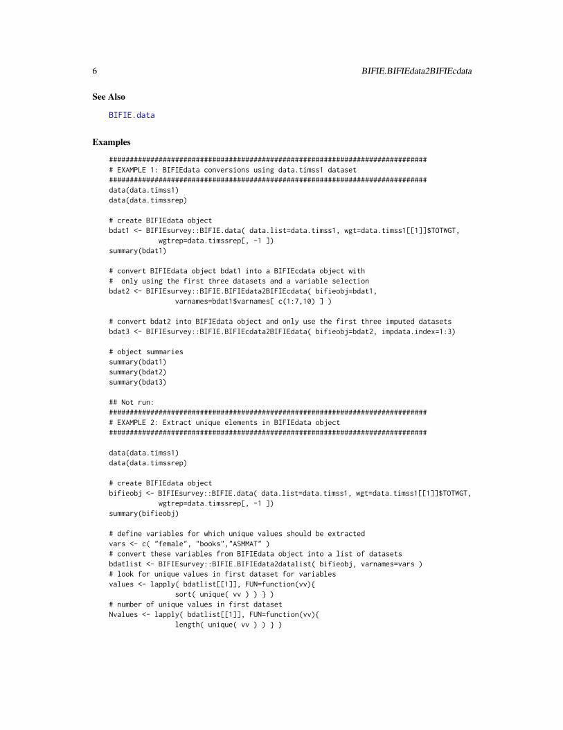
Functions for converting and selecting objects of class BIFIEdata. The function BIFIE.BIFIEdata2BIFIEcdataconverts the BIFIEdata objects in a non-compact form (cdata=FALSE) into an object of classBIFIEdata in a compact form (cdata=TRUE). The function BIFIE.BIFIE2data2BIFIEdata takesthe reverse operation.
The function BIFIE.BIFIEdata2datalist converts a (part) of the object of class BIFIEdata intoa list of multiply-imputed datasets.
Usage
BIFIE.BIFIEdata2BIFIEcdata(bifieobj, varnames=NULL, impdata.index=NULL)
BIFIE.BIFIEcdata2BIFIEdata(bifieobj, varnames=NULL, impdata.index=NULL)
BIFIE.BIFIEdata2datalist(bifieobj, varnames=NULL, impdata.index=NULL,as_data_frame=FALSE)
Arguments
bifieobj Object of class BIFIEdata
varnames Variables chosen for the selection
impdata.index Selected indices of imputed datasets
as_data_frame Logical indicating whether list of length one should be converted into a dataframe
Value
An object of class BIFIEdata saved in a non-compact or compact way, see value cdata.
6 BIFIE.BIFIEdata2BIFIEcdata
See Also
BIFIE.data
Examples
############################################################################## EXAMPLE 1: BIFIEdata conversions using data.timss1 dataset#############################################################################data(data.timss1)data(data.timssrep)
# create BIFIEdata objectbdat1 <- BIFIEsurvey::BIFIE.data( data.list=data.timss1, wgt=data.timss1[[1]]$TOTWGT,
wgtrep=data.timssrep[, -1 ])summary(bdat1)
# convert BIFIEdata object bdat1 into a BIFIEcdata object with# only using the first three datasets and a variable selectionbdat2 <- BIFIEsurvey::BIFIE.BIFIEdata2BIFIEcdata( bifieobj=bdat1,
varnames=bdat1$varnames[ c(1:7,10) ] )
# convert bdat2 into BIFIEdata object and only use the first three imputed datasetsbdat3 <- BIFIEsurvey::BIFIE.BIFIEcdata2BIFIEdata( bifieobj=bdat2, impdata.index=1:3)
# object summariessummary(bdat1)summary(bdat2)summary(bdat3)
## Not run:############################################################################## EXAMPLE 2: Extract unique elements in BIFIEdata object#############################################################################
data(data.timss1)data(data.timssrep)
# create BIFIEdata objectbifieobj <- BIFIEsurvey::BIFIE.data( data.list=data.timss1, wgt=data.timss1[[1]]$TOTWGT,
wgtrep=data.timssrep[, -1 ])summary(bifieobj)
# define variables for which unique values should be extractedvars <- c( "female", "books","ASMMAT" )# convert these variables from BIFIEdata object into a list of datasetsbdatlist <- BIFIEsurvey::BIFIE.BIFIEdata2datalist( bifieobj, varnames=vars )# look for unique values in first dataset for variablesvalues <- lapply( bdatlist[[1]], FUN=function(vv){
sort( unique( vv ) ) } )# number of unique values in first datasetNvalues <- lapply( bdatlist[[1]], FUN=function(vv){
length( unique( vv ) ) } )
BIFIE.by 7
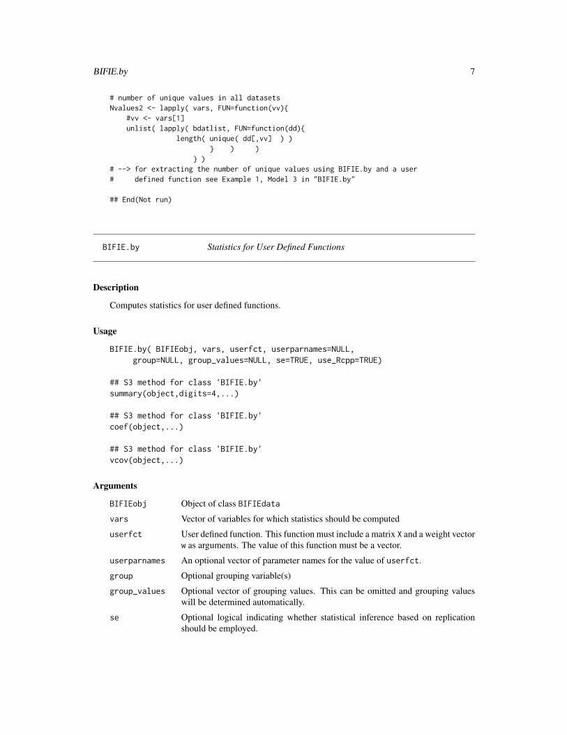
# number of unique values in all datasetsNvalues2 <- lapply( vars, FUN=function(vv){
#vv <- vars[1]unlist( lapply( bdatlist, FUN=function(dd){
length( unique( dd[,vv] ) )} ) )
} )# --> for extracting the number of unique values using BIFIE.by and a user# defined function see Example 1, Model 3 in "BIFIE.by"
## End(Not run)
BIFIE.by Statistics for User Defined Functions
Description
Computes statistics for user defined functions.
Usage
BIFIE.by( BIFIEobj, vars, userfct, userparnames=NULL,group=NULL, group_values=NULL, se=TRUE, use_Rcpp=TRUE)
## S3 method for class 'BIFIE.by'summary(object,digits=4,...)
## S3 method for class 'BIFIE.by'coef(object,...)
## S3 method for class 'BIFIE.by'vcov(object,...)
Arguments
BIFIEobj Object of class BIFIEdata
vars Vector of variables for which statistics should be computed
userfct User defined function. This function must include a matrix X and a weight vectorw as arguments. The value of this function must be a vector.
userparnames An optional vector of parameter names for the value of userfct.
group Optional grouping variable(s)
group_values Optional vector of grouping values. This can be omitted and grouping valueswill be determined automatically.
se Optional logical indicating whether statistical inference based on replicationshould be employed.
8 BIFIE.by
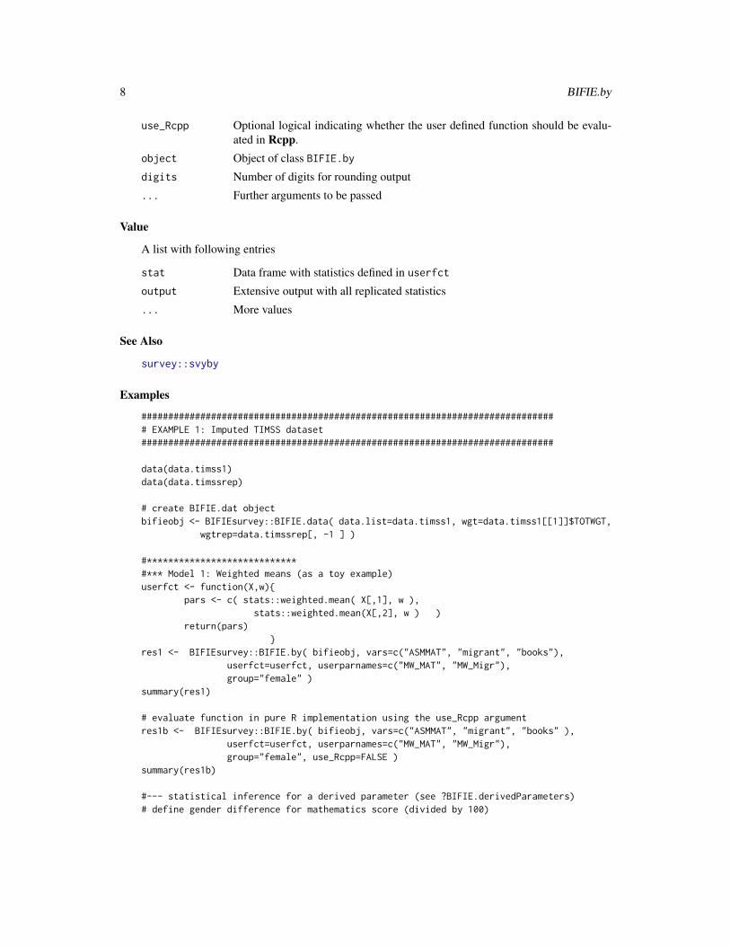
use_Rcpp Optional logical indicating whether the user defined function should be evalu-ated in Rcpp.
object Object of class BIFIE.by
digits Number of digits for rounding output
... Further arguments to be passed
Value
A list with following entries
stat Data frame with statistics defined in userfct
output Extensive output with all replicated statistics
... More values
See Also
survey::svyby
Examples
############################################################################## EXAMPLE 1: Imputed TIMSS dataset#############################################################################
data(data.timss1)data(data.timssrep)
# create BIFIE.dat objectbifieobj <- BIFIEsurvey::BIFIE.data( data.list=data.timss1, wgt=data.timss1[[1]]$TOTWGT,
wgtrep=data.timssrep[, -1 ] )
#****************************#*** Model 1: Weighted means (as a toy example)userfct <- function(X,w){
pars <- c( stats::weighted.mean( X[,1], w ),stats::weighted.mean(X[,2], w ) )
return(pars)}
res1 <- BIFIEsurvey::BIFIE.by( bifieobj, vars=c("ASMMAT", "migrant", "books"),userfct=userfct, userparnames=c("MW_MAT", "MW_Migr"),group="female" )
summary(res1)
# evaluate function in pure R implementation using the use_Rcpp argumentres1b <- BIFIEsurvey::BIFIE.by( bifieobj, vars=c("ASMMAT", "migrant", "books" ),
userfct=userfct, userparnames=c("MW_MAT", "MW_Migr"),group="female", use_Rcpp=FALSE )
summary(res1b)
#--- statistical inference for a derived parameter (see ?BIFIE.derivedParameters)# define gender difference for mathematics score (divided by 100)
BIFIE.by 9
derived.parameters <- list("gender_diff"=~ 0 + I( ( MW_MAT_female1 - MW_MAT_female0 ) / 100 )
)# inference derived parameterres1d <- BIFIEsurvey::BIFIE.derivedParameters( res1,
derived.parameters=derived.parameters )summary(res1d)
## Not run:#****************************#**** Model 2: Robust linear model
# (1) start from scratch to formulate the user function for X and wdat1 <- bifieobj$dat1vars <- c("ASMMAT", "migrant", "books" )X <- dat1[,vars]w <- bifieobj$wgtlibrary(MASS)# ASMMAT ~ migrant + booksmod <- MASS::rlm( X[,1] ~ as.matrix( X[, -1 ] ), weights=w )coef(mod)# (2) define a user function "my_rlm"my_rlm <- function(X,w){
mod <- MASS::rlm( X[,1] ~ as.matrix( X[, -1 ] ), weights=w )return( coef(mod) )
}# (3) estimate modelres2 <- BIFIEsurvey::BIFIE.by( bifieobj, vars, userfct=my_rlm,
group="female", group_values=0:1)summary(res2)# estimate model without computing standard errorsres2a <- BIFIEsurvey::BIFIE.by( bifieobj, vars, userfct=my_rlm,
group="female", se=FALSE)summary(res2a)
# define a user function with formula languagemy_rlm2 <- function(X,w){
colnames(X) <- varsX <- as.data.frame(X)mod <- MASS::rlm( ASMMAT ~ migrant + books, weights=w, data=X)return( coef(mod) )
}# estimate modelres2b <- BIFIEsurvey::BIFIE.by( bifieobj, vars, userfct=my_rlm2,
group="female", group_values=0:1)summary(res2b)
#****************************#**** Model 3: Number of unique values for variables in BIFIEdata
#*** define variables for which the number of unique values should be calculatedvars <- c( "female", "books","ASMMAT" )
10 BIFIE.by
#*** define a user function extracting these unqiue valuesuserfct <- function(X,w){
pars <- apply( X, 2, FUN=function(vv){length( unique(vv)) } )
# Note that weights are (of course) ignored in this functionreturn(pars)
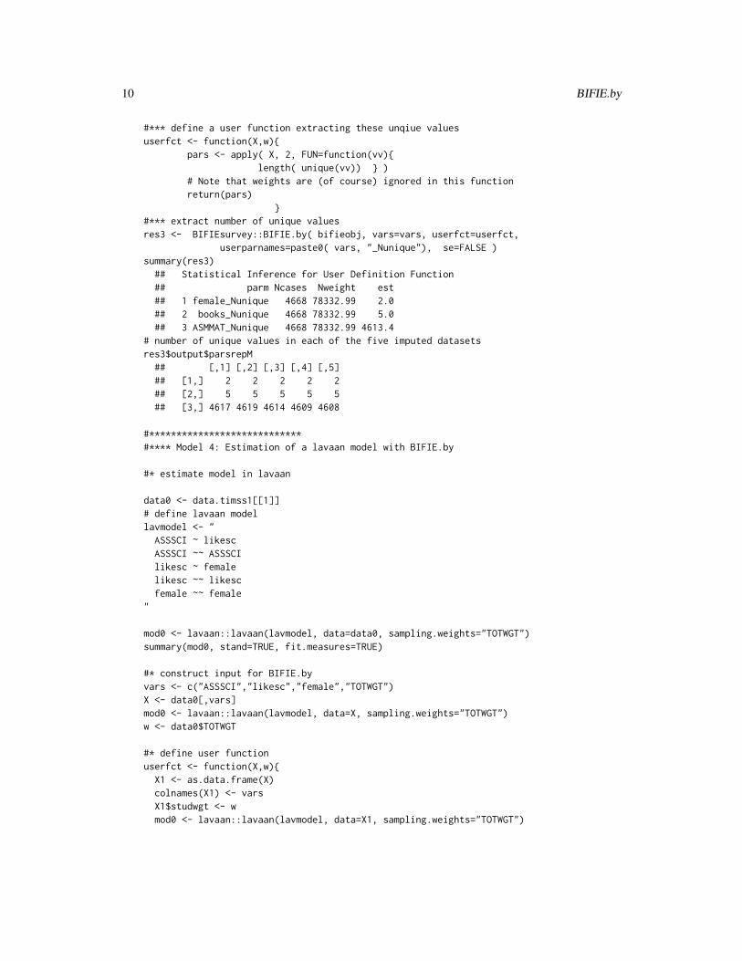
}#*** extract number of unique valuesres3 <- BIFIEsurvey::BIFIE.by( bifieobj, vars=vars, userfct=userfct,
userparnames=paste0( vars, "_Nunique"), se=FALSE )summary(res3)
## Statistical Inference for User Definition Function## parm Ncases Nweight est## 1 female_Nunique 4668 78332.99 2.0## 2 books_Nunique 4668 78332.99 5.0## 3 ASMMAT_Nunique 4668 78332.99 4613.4
# number of unique values in each of the five imputed datasetsres3$output$parsrepM
## [,1] [,2] [,3] [,4] [,5]## [1,] 2 2 2 2 2## [2,] 5 5 5 5 5## [3,] 4617 4619 4614 4609 4608
#****************************#**** Model 4: Estimation of a lavaan model with BIFIE.by
#* estimate model in lavaan
data0 <- data.timss1[[1]]# define lavaan modellavmodel <- "
ASSSCI ~ likescASSSCI ~~ ASSSCIlikesc ~ femalelikesc ~~ likescfemale ~~ female
"
mod0 <- lavaan::lavaan(lavmodel, data=data0, sampling.weights="TOTWGT")summary(mod0, stand=TRUE, fit.measures=TRUE)
#* construct input for BIFIE.byvars <- c("ASSSCI","likesc","female","TOTWGT")X <- data0[,vars]mod0 <- lavaan::lavaan(lavmodel, data=X, sampling.weights="TOTWGT")w <- data0$TOTWGT
#* define user functionuserfct <- function(X,w){
X1 <- as.data.frame(X)colnames(X1) <- varsX1$studwgt <- wmod0 <- lavaan::lavaan(lavmodel, data=X1, sampling.weights="TOTWGT")
BIFIE.correl 11
pars <- coef(mod0)# extract some fit statisticspars2 <- lavaan::fitMeasures(mod0)pars <- c(pars, pars2[c("cfi","tli")])return(pars)
}
#* test functionres0 <- userfct(X,w)userparnames <- names(res0)
#* estimate lavaan model with replicated sampling weightsres1 <- BIFIEsurvey::BIFIE.by( bifieobj, vars=vars, userfct=userfct,
userparnames=userparnames, use_Rcpp=FALSE )summary(res1)
## End(Not run)
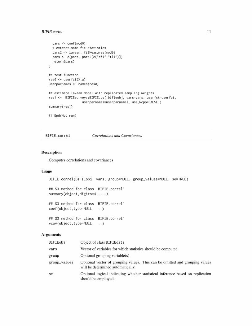
BIFIE.correl Correlations and Covariances
Description
Computes correlations and covariances
Usage
BIFIE.correl(BIFIEobj, vars, group=NULL, group_values=NULL, se=TRUE)
## S3 method for class 'BIFIE.correl'summary(object,digits=4, ...)
## S3 method for class 'BIFIE.correl'coef(object,type=NULL, ...)
## S3 method for class 'BIFIE.correl'vcov(object,type=NULL, ...)
Arguments
BIFIEobj Object of class BIFIEdata
vars Vector of variables for which statistics should be computed
group Optional grouping variable(s)
group_values Optional vector of grouping values. This can be omitted and grouping valueswill be determined automatically.
se Optional logical indicating whether statistical inference based on replicationshould be employed.
12 BIFIE.correl
object Object of class BIFIE.correl
digits Number of digits for rounding output
type If type="cov", then covariances instead of correlations are extracted.
... Further arguments to be passed
Value
A list with following entries
stat.cor Data frame with correlation statistics
stat.cov Data frame with covariance statistics
cor_matrix List of estimated correlation matrices
cov_matrix List of estimated covariance matrices
output Extensive output with all replicated statistics
... More values
See Also
stats::cov.wt, intsvy::timss.rho, intsvy::timss.rho.pv, Hmisc::rcorr, miceadds::ma.wtd.corNA
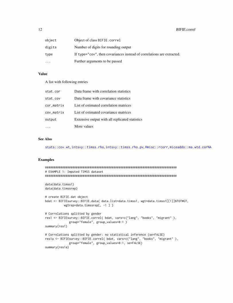
Examples
############################################################################## EXAMPLE 1: Imputed TIMSS dataset#############################################################################
data(data.timss1)data(data.timssrep)
# create BIFIE.dat objectbdat <- BIFIEsurvey::BIFIE.data( data.list=data.timss1, wgt=data.timss1[[1]]$TOTWGT,
wgtrep=data.timssrep[, -1 ] )
# Correlations splitted by genderres1 <- BIFIEsurvey::BIFIE.correl( bdat, vars=c("lang", "books", "migrant" ),
group="female", group_values=0:1 )summary(res1)
# Correlations splitted by gender: no statistical inference (se=FALSE)res1a <- BIFIEsurvey::BIFIE.correl( bdat, vars=c("lang", "books", "migrant" ),
group="female", group_values=0:1, se=FALSE)summary(res1a)
BIFIE.crosstab 13
BIFIE.crosstab Cross Tabulation
Description
Creates cross tabulations and computes some effect sizes.
Usage
BIFIE.crosstab( BIFIEobj, vars1, vars2, vars_values1=NULL, vars_values2=NULL,group=NULL, group_values=NULL, se=TRUE )
## S3 method for class 'BIFIE.crosstab'summary(object,digits=3,...)
## S3 method for class 'BIFIE.crosstab'coef(object,...)
## S3 method for class 'BIFIE.crosstab'vcov(object,...)
Arguments
BIFIEobj Object of class BIFIEdata
vars1 Row variable
vars2 Column variable
vars_values1 Optional vector of values of variable vars1
vars_values2 Optional vector of values of variable vars2
group Optional grouping variable(s)
group_values Optional vector of grouping values. This can be omitted and grouping valueswill be determined automatically.
se Optional logical indicating whether statistical inference based on replicationshould be employed.
object Object of class BIFIE.univar
digits Number of digits for rounding output
... Further arguments to be passed
Value
A list with following entries
stat.probs Statistics for joint and conditional probabilities
stat.marg Statistics for marginal probabilities
14 BIFIE.data
stat.es Statistics for effect sizes w (based on χ2), Cramers V , Goodman’s gamma, thePRE lambda measure and Kruskals tau.
output Extensive output with all replicated statistics
... More values
See Also
survey::svytable, Hmisc::wtd.table
Examples
############################################################################## EXAMPLE 1: Imputed TIMSS dataset#############################################################################
data(data.timss1)data(data.timssrep)
# create BIFIE.dat objectbifieobj <- BIFIEsurvey::BIFIE.data( data.list=data.timss1, wgt=data.timss1[[1]]$TOTWGT,
wgtrep=data.timssrep[, -1 ] )
#--- Model 1: cross tabulationres1 <- BIFIEsurvey::BIFIE.crosstab( bifieobj, vars1="migrant",
vars2="books", group="female" )summary(res1)
BIFIE.data Creates an Object of Class BIFIEdata
Description
This function creates an object of class BIFIEdata. Finite sampling correction of statistical infer-ences can be conducted by specifying appropriate input in the fayfac argument.
Usage
BIFIE.data(data.list, wgt=NULL, wgtrep=NULL, fayfac=1, pv_vars=NULL,pvpre=NULL, cdata=FALSE, NMI=FALSE)
## S3 method for class 'BIFIEdata'summary(object,...)
## S3 method for class 'BIFIEdata'print(x,...)
BIFIE.data 15
Arguments
data.list List of multiply imputed datasets. Can be also a list of list of imputed datasetsin case of nested multiple imputation. Then, the argument NMI=TRUE must bespecified.
wgt A string indicating the label of case weight or a vector containing all caseweights.
wgtrep Optional vector of replicate weightsfayfac Fay factor for calculating standard errors, a numeric value. If finite sampling
correction is requested, an appropriate vector input can be used (see Example3).
pv_vars Optional vector for names of plausible values, see BIFIE.data.jack.pvpre Optional vector for prefixes of plausible values, see BIFIE.data.jack.cdata An optional logical indicating whether the BIFIEdata object should be com-
pactly saved. The default is FALSE.NMI Optional logical indicating whether data.list is obtained by nested multiple
imputation.object Object of class BIFIEdatax Object of class BIFIEdata... Further arguments to be passed
Value
An object of class BIFIEdata saved in a non-compact or compact way, see value cdata. Thefollowing entries are included in the list:
datalistM Stacked list of imputed datasets (if cdata=FALSE)wgt Vector with case weightswgtrep Matrix with replicate weightsNimp Number of imputed datasetsN Number of observations in a datasetdat1 Last imputed datasetvarnames Vector with variable namesfayfac Fay factor.RR Number of replicate weightsNMI Logical indicating whether the dataset is nested multiply imputed.cdata Logical indicating whether the BIFIEdata object is in compact format (cdata=TRUE)
or in a non-compact format (cdata=FALSE).Nvars Number of variablesvariables Data frame including some informations about variables. All transformations
are saved in the column source.datalistM_ind Data frame with response indicators (if cdata=TRUE)datalistM_imputed
Data frame with imputed values (if cdata=TRUE)
16 BIFIE.data
See Also
See BIFIE.data.transform for data transformations on BIFIEdata objects.
For saving and loading BIFIEdata objects see save.BIFIEdata.
For converting PIRLS/TIMSS or PISA datasets into BIFIEdata objects see BIFIE.data.jack.
See the BIFIEdata2svrepdesign function for converting BIFIEdata objects to objects used in thesurvey package.
Examples
############################################################################## EXAMPLE 1: Create BIFIEdata object with multiply-imputed TIMSS data#############################################################################data(data.timss1)data(data.timssrep)
bdat <- BIFIEsurvey::BIFIE.data( data.list=data.timss1, wgt=data.timss1[[1]]$TOTWGT,wgtrep=data.timssrep[, -1 ] )
summary(bdat)# create BIFIEdata object in a compact waybdat2 <- BIFIEsurvey::BIFIE.data( data.list=data.timss1, wgt=data.timss1[[1]]$TOTWGT,
wgtrep=data.timssrep[, -1 ], cdata=TRUE)summary(bdat2)
## Not run:############################################################################## EXAMPLE 2: Create BIFIEdata object with one dataset#############################################################################data(data.timss2)
# use first dataset with missing data from data.timss2bdat <- BIFIEsurvey::BIFIE.data( data.list=data.timss2[[1]], wgt=data.timss2[[1]]$TOTWGT)
## End(Not run)
############################################################################## EXAMPLE 3: BIFIEdata objects with finite sampling correction#############################################################################
data(data.timss1)data(data.timssrep)
#-----# BIFIEdata object without finite sampling correctionbdat1 <- BIFIEsurvey::BIFIE.data( data.list=data.timss1, wgt=data.timss1[[1]]$TOTWGT,
wgtrep=data.timssrep[, -1 ] )summary(bdat1)
#-----# generate BIFIEdata object with finite sampling correction by adjusting# the "fayfac" factorbdat2 <- bdat1
BIFIE.data.boot 17
#-- modify "fayfac" constantfayfac0 <- bdat1$fayfac# set fayfac=.75 for the first 50 replication zones (25% of students in the# population were sampled) and fayfac=.20 for replication zones 51-75# (meaning that 80% of students were sampled)fayfac <- rep( fayfac0, bdat1$RR )fayfac[1:50] <- fayfac0 * .75fayfac[51:75] <- fayfac0 * .20# include this modified "fayfac" factor in bdat2bdat2$fayfac <- fayfacsummary(bdat2)summary(bdat1)
#---- compare some univariate statistics# no finite sampling correctionres1 <- BIFIEsurvey::BIFIE.univar( bdat1, vars="ASMMAT")summary(res1)# finite sampling correctionres2 <- BIFIEsurvey::BIFIE.univar( bdat2, vars="ASMMAT")summary(res2)
## Not run:############################################################################## EXAMPLE 4: Create BIFIEdata object with nested multiply imputed dataset#############################################################################
data(data.timss4)data(data.timssrep)
# nested imputed dataset, save it in compact formatbdat <- BIFIEsurvey::BIFIE.data( data.list=data.timss4,
wgt=data.timss4[[1]][[1]]$TOTWGT, wgtrep=data.timssrep[, -1 ],NMI=TRUE, cdata=TRUE )
summary(bdat)
## End(Not run)
BIFIE.data.boot Create BIFIE.data Object based on Bootstrap
Description
Creates a BIFIE.data object based on bootstrap designs. The sampling is done assuming indepen-dence of cases.
Usage
BIFIE.data.boot( data, wgt=NULL, pv_vars=NULL,Nboot=500, seed=.Random.seed, cdata=FALSE)
18 BIFIE.data.jack
Arguments
data Data frame: Can be a single or a list of multiply imputed datasets
wgt A string indicating the label of case weight.
pv_vars An optional vector of plausible values which define multiply imputed datasets.
Nboot Number of bootstrap samples for usage
seed Simulation seed.
cdata An optional logical indicating whether the BIFIEdata object should be com-pactly saved. The default is FALSE.
Value
Object of class BIFIEdata
See Also
BIFIE.data, BIFIE.data.jack
Examples
## Not run:############################################################################## EXAMPLE 1: Bootstrap TIMSS data set#############################################################################data(data.timss1)
# bootstrap samples using weightsbifieobj1 <- BIFIEsurvey::BIFIE.data.boot( data.timss1, wgt="TOTWGT" )summary(bifieobj1)
# bootstrap samples without weightsbifieobj2 <- BIFIEsurvey::BIFIE.data.boot( data.timss1 )summary(bifieobj2)
## End(Not run)
BIFIE.data.jack Create BIFIE.data Object with Jackknife Zones
Description
Creates a BIFIE.data object for designs with jackknife zones, especially for TIMSS/PIRLS andPISA studies.
BIFIE.data.jack 19
Usage
BIFIE.data.jack(data, wgt=NULL, jktype="JK_TIMSS", pv_vars=NULL,jkzone=NULL, jkrep=NULL, jkfac=NULL, fayfac=NULL,wgtrep="W_FSTR", pvpre=paste0("PV",1:5), ngr=100,seed=.Random.seed, cdata=FALSE)
Arguments
data Data frame: Can be a single or a list of multiply-imputed datasets
wgt A string indicating the label of case weight. In case of jktype="JK_TIMSS" theweight is specified as wgt="TOTWGT" as the default.
pv_vars An optional vector of plausible values which define multiply-imputed datasets.
jktype Type of jackknife procedure for creating the BIFIE.data object. jktype="JK_TIMSS"refers to TIMSS/PIRLS datasets up to 2011 data, jktype="JK_TIMSS2" refersto TIMSS/PIRLS datasets starting from 2015 data. The type "JK_GROUP" cre-ates jackknife weights based on a user defined grouping, the type "JK_RANDOM"creates random groups. The number of random groups can be defined in ngr.The argument type="RW_PISA" converts PISA datasets into objects of classBIFIEdata.
jkzone Jackknife zones. If jktype="JK_TIMSS", then jkzone="JKZONE".
jkrep Jackknife replicate factors. If jktype="JK_TIMSS", then jkrep="JKREP".
jkfac Factor for multiplying jackknife replicate weights. If jktype="JK_TIMSS", thenjkfac=2.
fayfac Fay factor for statistical inference. The default is set to NULL.
wgtrep Variables in the dataset which refer to the replicate weights. In case of cdata=TRUE,the replicate weights are deleted from datalistM.
pvpre Only applicable for jktype="RW_PISA". The vector contains the prefixes of thevariables containing plausible values.
ngr Number of randomly created groups in "JK_RANDOM".
seed The simulation seed if "JK_RANDOM" is chosen. If seed=NULL, then the groupingis done according the order in the dataset.
cdata An optional logical indicating whether the BIFIEdata object should be com-pactly saved. The default is FALSE.
Value
Object of class BIFIEdata
See Also
BIFIE.data, BIFIE.data.boot
20 BIFIE.data.jack
Examples
############################################################################## EXAMPLE 1: Convert TIMSS dataset to BIFIE.data object#############################################################################
data(data.timss3)
# define plausible valuespv_vars <- c("ASMMAT", "ASSSCI" )# create BIFIE.data objects -> 5 imputed datasetsbdat1 <- BIFIEsurvey::BIFIE.data.jack( data=data.timss3, pv_vars=pv_vars,
jktype="JK_TIMSS" )summary(bdat1)
# create BIFIE.data objects -> all PVs are included in one datasetbdat2 <- BIFIEsurvey::BIFIE.data.jack( data=data.timss3, jktype="JK_TIMSS" )summary(bdat2)
############################################################################## EXAMPLE 2: Creation of Jackknife zones and replicate weights for data.test1#############################################################################
data(data.test1)
# create jackknife zones based on random group creationbdat1 <- BIFIEsurvey::BIFIE.data.jack( data=data.test1, jktype="JK_RANDOM",
ngr=50 )summary(bdat1)stat1 <- BIFIEsurvey::BIFIE.univar( bdat1, vars="math", group="stratum" )summary(stat1)
# random creation of groups and inclusion of weightsbdat2 <- BIFIEsurvey::BIFIE.data.jack( data=data.test1, jktype="JK_RANDOM",
ngr=75, seed=987, wgt="wgtstud")summary(bdat2)stat2 <- BIFIEsurvey::BIFIE.univar( bdat2, vars="math", group="stratum" )summary(stat2)
# using idclass as jackknife zonesbdat3 <- BIFIEsurvey::BIFIE.data.jack( data=data.test1, jktype="JK_GROUP",
jkzone="idclass", wgt="wgtstud")summary(bdat3)stat3 <- BIFIEsurvey::BIFIE.univar( bdat3, vars="math", group="stratum" )summary(stat3)
# create BIFIEdata object with a list of imputed datasetsdataList <- list( data.test1, data.test1, data.test1 )bdat4 <- BIFIEsurvey::BIFIE.data.jack( data=dataList, jktype="JK_GROUP",
jkzone="idclass", wgt="wgtstud")summary(bdat4)
## Not run:
BIFIE.data.transform 21
############################################################################## EXAMPLE 3: Converting a PISA dataset into a BIFIEdata object#############################################################################
data(data.pisaNLD)
# BIFIEdata with cdata=FALSEbifieobj <- BIFIEsurvey::BIFIE.data.jack( data.pisaNLD, jktype="RW_PISA", cdata=FALSE)summary(bifieobj)# BIFIEdata with cdata=TRUEbifieobj1 <- BIFIEsurvey::BIFIE.data.jack( data.pisaNLD, jktype="RW_PISA", cdata=TRUE)summary(bifieobj1)
## End(Not run)
BIFIE.data.transform Data Transformation for BIFIEdata Objects
Description
Computes a data transformation for BIFIEdata objects.
Usage
BIFIE.data.transform( bifieobj, transform.formula, varnames.new=NULL )
Arguments
bifieobj Object of class BIFIEdatatransform.formula
R formula object for data transformation.
varnames.new Optional vector of names for new defined variables.
Value
An object of class BIFIEdata. Additional values are
varnames.added Added variables in data transformationvarsindex.added
Indices of added variables
Examples
library(miceadds)
############################################################################## EXAMPLE 1: Data transformations for TIMSS data#############################################################################
22 BIFIE.data.transform
data(data.timss2)data(data.timssrep)# create BIFIEdata objectbifieobj1 <- BIFIEsurvey::BIFIE.data( data.timss2, wgt=data.timss2[[1]]$TOTWGT,
wgtrep=data.timssrep[,-1] )# create BIFIEdata object in compact way (cdata=TRUE)bifieobj2 <- BIFIEsurvey::BIFIE.data( data.timss2, wgt=data.timss2[[1]]$TOTWGT,
wgtrep=data.timssrep[,-1], cdata=TRUE)
#****************************#*** Transformation 1: Squared and cubic book variabletransform.formula <- ~ I( books^2 ) + I( books^3 )# as.character(transform.formula)bifieobj <- BIFIEsurvey::BIFIE.data.transform( bifieobj1,
transform.formula=transform.formula)bifieobj$variables# rename added variablesbifieobj$varnames[ bifieobj$varsindex.added ] <- c("books_sq", "books_cub")
# check descriptive statisticsres1 <- BIFIEsurvey::BIFIE.univar( bifieobj, vars=c("books_sq", "books_cub" ) )summary(res1)
## Not run:#****************************#*** Transformation 2: Create dummy variables for variable booktransform.formula <- ~ as.factor(books)bifieobj <- BIFIEsurvey::BIFIE.data.transform( bifieobj,
transform.formula=transform.formula )## Included 5 variables: as.factor(books)1 as.factor(books)2 as.factor(books)3## as.factor(books)4 as.factor(books)5bifieobj$varnames[ bifieobj$varsindex.added ] <- paste0("books_D", 1:5)
#****************************#*** Transformation 3: Discretized mathematics scorehi3a <- BIFIEsurvey::BIFIE.hist( bifieobj, vars="ASMMAT" )plot(hi3a)transform.formula <- ~ I( as.numeric(cut( ASMMAT, breaks=seq(200,800,100) )) )bifieobj <- BIFIEsurvey::BIFIE.data.transform( bifieobj,
transform.formula=transform.formula, varnames.new="ASMMAT_discret")hi3b <- BIFIEsurvey::BIFIE.hist( bifieobj, vars="ASMMAT_discret", breaks=1:7 )plot(hi3b)# check frequenciesfr3b <- BIFIEsurvey::BIFIE.freq( bifieobj, vars="ASMMAT_discret", se=FALSE )summary(fr3b)
#****************************#*** Transformation 4: include standardization variables for book variable
# start with testing the transformation function on a single datasetdat1 <- bifieobj$dat1stats::weighted.mean( dat1[,"books"], dat1[,"TOTWGT"], na.rm=TRUE)sqrt( Hmisc::wtd.var( dat1[,"books"], dat1[,"TOTWGT"], na.rm=TRUE) )
BIFIE.data.transform 23
# z standardizationtransform.formula <- ~ I( ( books - weighted.mean( books, TOTWGT, na.rm=TRUE) )/
sqrt( Hmisc::wtd.var( books, TOTWGT, na.rm=TRUE) ))bifieobj <- BIFIEsurvey::BIFIE.data.transform( bifieobj,
transform.formula=transform.formula, varnames.new="z_books" )# standardize variable books with M=500 and SD=100transform.formula <- ~ I(
500 + 100*( books - stats::weighted.mean( books, w=TOTWGT, na.rm=TRUE) ) /sqrt( Hmisc::wtd.var( books, weights=TOTWGT, na.rm=TRUE) ) )
bifieobj <- BIFIEsurvey::BIFIE.data.transform( bifieobj,transform.formula=transform.formula, varnames.new="z500_books" )
# standardize variable books with respect to M and SD of ALL imputed datasetsres <- BIFIEsurvey::BIFIE.univar( bifieobj, vars="books" )summary(res)## var Nweight Ncases M M_SE M_fmi M_VarMI M_VarRep SD SD_SE SD_fmi## 1 books 76588.72 4554 2.945 0.04 0 0 0.002 1.146 0.015 0M <- round(res$output$mean1,5)SD <- round(res$output$sd1,5)transform.formula <- paste0( " ~ I( ( books - ", M, " ) / ", SD, ")" )## > transform.formula## [1] " ~ I( ( books - 2.94496 ) / 1.14609)"bifieobj <- BIFIEsurvey::BIFIE.data.transform( bifieobj,
transform.formula=stats::as.formula(transform.formula),varnames.new="zall_books" )
# check statisticsres4 <- BIFIEsurvey::BIFIE.univar( bifieobj,
vars=c("z_books", "z500_books", "zall_books") )summary(res4)
#****************************#*** Transformation 5: include rank transformation for variable ASMMAT
# calculate percentage ranks using wtd.rank function from Hmisc packagedat1 <- bifieobj$dat1100 * Hmisc::wtd.rank( dat1[,"ASMMAT"], w=dat1[,"TOTWGT"] ) / sum( dat1[,"TOTWGT"] )# define an auxiliary function for calculating percentage rankswtd.percrank <- function( x, w ){
100 * Hmisc::wtd.rank( x, w, na.rm=TRUE ) / sum( w, na.rm=TRUE )}wtd.percrank( dat1[,"ASMMAT"], dat1[,"TOTWGT"] )# define transformation formulatransform.formula <- ~ I( wtd.percrank( ASMMAT, TOTWGT ) )# add ranks to BIFIEdata objectbifieobj <- BIFIEsurvey::BIFIE.data.transform( bifieobj,
transform.formula=transform.formula, varnames.new="ASMMAT_rk")# check statisticres5 <- BIFIEsurvey::BIFIE.univar( bifieobj, vars=c("ASMMAT_rk" ) )summary(res5)
#****************************#*** Transformation 6: recode variable books
24 BIFIE.data.transform
library(car)# recode variable books according to "1,2=0, 3,4=1, 5=2"dat1 <- bifieobj$dat1# use Recode function from car packagecar::Recode( dat1[,"books"], "1:2='0'; c(3,4)='1';5='2'")# define transformation formulatransform.formula <- ~ I( car::Recode( books, "1:2='0'; c(3,4)='1';5='2'") )bifieobj <- BIFIEsurvey::BIFIE.data.transform( bifieobj,
transform.formula=transform.formula, varnames.new="book_rec" )res6 <- BIFIEsurvey::BIFIE.freq( bifieobj, vars=c("book_rec" ) )summary(res6)
#****************************#*** Transformation 7: include some variables aggregated to the school level
dat1 <- as.data.frame(bifieobj$dat1)# at first, create school ID in the dataset by transforming the student IDdat1$idschool <- as.numeric(substring( dat1$IDSTUD, 1, 5 ))transform.formula <- ~ I( as.numeric( substring( IDSTUD, 1, 5 ) ) )bifieobj <- BIFIEsurvey::BIFIE.data.transform( bifieobj,
transform.formula=transform.formula, varnames.new="idschool" )
#*** test function for a single dataset bifieobj$dat1dat1 <- as.data.frame(bifieobj$dat1)gm <- miceadds::GroupMean( data=dat1$ASMMAT, group=dat1$idschool, extend=TRUE)[,2]
# add school mean ASMMATtformula <- ~ I( miceadds::GroupMean( ASMMAT, group=idschool, extend=TRUE)[,2] )bifieobj <- BIFIEsurvey::BIFIE.data.transform( bifieobj, transform.formula=tformula,
varnames.new="M_ASMMAT" )# add within group centered mathematics values of ASMMATbifieobj <- BIFIEsurvey::BIFIE.data.transform( bifieobj,
transform.formula=~ 0 + I( ASMMAT - M_ASMMAT ),varnames.new="WC_ASMMAT" )
# add school mean booksbifieobj <- BIFIEsurvey::BIFIE.data.transform( bifieobj,
transform.formula=~ 0 + I( add.groupmean( books, idschool ) ),varnames.new="M_books" )
#****************************#*** Transformation 8: include fitted values and residuals from a linear model# create new BIFIEdata objectdata(data.timss1)bifieobj3 <- BIFIEsurvey::BIFIE.data( data.timss1, wgt=data.timss1[[1]]$TOTWGT,
wgtrep=data.timssrep[,-1] )
# specify transformationtransform.formula <- ~ I( fitted( stats::lm( ASMMAT ~ migrant + female ) ) ) +
I( residuals( stats::lm( ASMMAT ~ migrant + female ) ) )# Note that lm omits cases in regression by listwise deletion.
# add fitted values and residual to BIFIEdata object
BIFIE.derivedParameters 25
bifieobj <- BIFIEsurvey::BIFIE.data.transform( bifieobj3,transform.formula=transform.formula )
bifieobj$varnames[ bifieobj$varsindex.added ] <- c("math_fitted1", "math_resid1")
#****************************#*** Transformation 9: Including principal component scores in BIFIEdata object
# define auxiliary function for extracting PCA scoresBIFIE.princomp <- function( formula, Ncomp ){
X <- stats::princomp( formula, cor=TRUE)Xp <- X$scores[, 1:Ncomp ]return(Xp)
}# define transformation formulatransform.formula <- ~ I( BIFIE.princomp( ~ migrant + female + books + lang + ASMMAT, 3 ))# apply transformationbifieobj <- BIFIEsurvey::BIFIE.data.transform( bifieobj3,
transform.formula=transform.formula )bifieobj$varnames[ bifieobj$varsindex.added ] <- c("pca_sc1", "pca_sc2","pca_sc3")# check descriptive statisticsres9 <- BIFIEsurvey::BIFIE.univar( bifieobj, vars="pca_sc1", se=FALSE)summary(res9)res9$output$mean1M
# The transformation formula can also be conveniently generated by string operationsvars <- c("migrant", "female", "books", "lang" )transform.formula2 <- as.formula( paste0( "~ 0 + I ( BIFIE.princomp( ~ ",
paste0( vars, collapse="+" ), ", 3 ) )") )## > transform.formula2## ~ I(BIFIE.princomp(~migrant + female + books + lang, 3))
#****************************#*** Transformation 10: Overwriting variables books and migrantbifieobj4 <- BIFIEsurvey::BIFIE.data.transform( bifieobj3,
transform.formula=~ I( 1*(books >=1 ) ) + I(2*migrant),varnames.new=c("books","migrant") )
summary(bifieobj4)
## End(Not run)
BIFIE.derivedParameters
Statistical Inference for Derived Parameters
Description
This function performs statistical for derived parameters for objects of classes BIFIE.by, BIFIE.correl,BIFIE.crosstab, BIFIE.freq, BIFIE.linreg, BIFIE.logistreg and BIFIE.univar.
26 BIFIE.derivedParameters
Usage
BIFIE.derivedParameters( BIFIE.method, derived.parameters, type=NULL)
## S3 method for class 'BIFIE.derivedParameters'summary(object,digits=4,...)
## S3 method for class 'BIFIE.derivedParameters'coef(object,...)
## S3 method for class 'BIFIE.derivedParameters'vcov(object,...)
Arguments
BIFIE.method Object of classes BIFIE.by, BIFIE.correl, BIFIE.crosstab, BIFIE.freq,BIFIE.linreg, BIFIE.logistreg or BIFIE.univar (see parnames in the Out-put of these methods for saved parameters)
derived.parameters
List with R formulas for derived parameters (see Examples for specification)
type Only applies to BIFIE.correl. In case of type="cov" covariances instead ofcorrelations are used for derived parameters.
object Object of class BIFIE.derivedParameters
digits Number of digits for rounding decimals in output
... Further arguments to be passed
Details
The distribution of derived parameters is derived by the direct calculation using original resampledparameters.
Value
A list with following entries
stat Data frame with statistics
coef Estimates of derived parameters
vcov Covariance matrix of derived parameters
parnames Parameter names
res_wald Output of Wald test (global test regarding all parameters)
... More values
See Also
See also BIFIE.waldtest for multi-parameter tests.
See car::deltaMethod for the Delta method assuming that the multivariate distribution of theparameters is asymptotically normal.
BIFIE.ecdf 27
Examples
############################################################################## EXAMPLE 1: Imputed TIMSS dataset# Inference for correlations and derived parameters#############################################################################
data(data.timss1)data(data.timssrep)
# create BIFIE.dat objectbdat <- BIFIEsurvey::BIFIE.data( data.list=data.timss1, wgt=data.timss1[[1]]$TOTWGT,
wgtrep=data.timssrep[, -1 ] )
# compute correlationsres1 <- BIFIEsurvey::BIFIE.correl( bdat,
vars=c("ASSSCI", "ASMMAT", "books", "migrant" ) )summary(res1)res1$parnames
## [1] "ASSSCI_ASSSCI" "ASSSCI_ASMMAT" "ASSSCI_books" "ASSSCI_migrant"## [5] "ASMMAT_ASMMAT" "ASMMAT_books" "ASMMAT_migrant" "books_books"## [9] "books_migrant" "migrant_migrant"
# define four derived parametersderived.parameters <- list(
# squared correlation of science and mathematics"R2_sci_mat"=~ I( 100* ASSSCI_ASMMAT^2 ),# partial correlation of science and mathematics controlling for books"parcorr_sci_mat"=~ I( ( ASSSCI_ASMMAT - ASSSCI_books * ASMMAT_books ) /
sqrt(( 1 - ASSSCI_books^2 ) * ( 1-ASMMAT_books^2 ) ) ),# original correlation science and mathematics (already contained in res1)"cor_sci_mat"=~ I(ASSSCI_ASMMAT),# original correlation books and migrant"cor_book_migra"=~ I(books_migrant))
# statistical inference for derived parametersres2 <- BIFIEsurvey::BIFIE.derivedParameters( res1, derived.parameters )summary(res2)
BIFIE.ecdf Empirical Distribution Function and Quantiles
Description
Computes an empirical distribution function (and quantiles). If only some quantiles should becalculated, then an appropriate vector of breaks (which are quantiles) must be specified. Statisticalinference is not conducted for this method.
28 BIFIE.ecdf
Usage
BIFIE.ecdf( BIFIEobj, vars, breaks=NULL, quanttype=1, group=NULL, group_values=NULL )
## S3 method for class 'BIFIE.ecdf'summary(object,digits=4,...)
Arguments
BIFIEobj Object of class BIFIEdata
vars Vector of variables for which statistics should be computed.
breaks Optional vector of breaks. Otherwise, it will be automatically defined.
quanttype Type of calculation for quantiles. In case of quanttype=1, a linear interpolationis used (which is type='i/n' in Hmisc::wtd.quantile), while for quanttype=2no interpolation is used.
group Optional grouping variable
group_values Optional vector of grouping values. This can be omitted and grouping valueswill be determined automatically.
object Object of class BIFIE.ecdf
digits Number of digits for rounding output
... Further arguments to be passed
Value
A list with following entries
ecdf Data frame with probabilities and the empirical distribution function (See Ex-amples).
stat Data frame with empirical distribution function stacked with respect to vari-ables, groups and group values
output More extensive output
... More values
See Also
Hmisc::wtd.ecdf, Hmisc::wtd.quantile
Examples
############################################################################## EXAMPLE 1: Imputed TIMSS dataset#############################################################################
data(data.timss1)data(data.timssrep)
# create BIFIE.dat object
BIFIE.freq 29
bifieobj <- BIFIEsurvey::BIFIE.data( data.list=data.timss1, wgt=data.timss1[[1]]$TOTWGT,wgtrep=data.timssrep[, -1 ] )
# ecdfvars <- c( "ASMMAT", "books")group <- "female" ; group_values <- 0:1# quantile type 1res1 <- BIFIEsurvey::BIFIE.ecdf( bifieobj, vars=vars, group=group )summary(res1)res2 <- BIFIEsurvey::BIFIE.ecdf( bifieobj, vars=vars, group=group, quanttype=2)# plot distribution functionecdf1 <- res1$ecdfplot( ecdf1$ASMMAT_female0, ecdf1$yval, type="l")plot( res2$ecdf$ASMMAT_female0, ecdf1$yval, type="l", lty=2)plot( ecdf1$books_female0, ecdf1$yval, type="l", col="blue")
BIFIE.freq Frequency Statistics
Description
Computes absolute and relative frequencies.
Usage
BIFIE.freq(BIFIEobj, vars, group=NULL, group_values=NULL, se=TRUE)
## S3 method for class 'BIFIE.freq'summary(object,digits=3,...)
## S3 method for class 'BIFIE.freq'coef(object,...)
## S3 method for class 'BIFIE.freq'vcov(object,...)
Arguments
BIFIEobj Object of class BIFIEdatavars Vector of variables for which statistics should be computedgroup Optional grouping variable(s)group_values Optional vector of grouping values. This can be omitted and grouping values
will be determined automatically.se Optional logical indicating whether statistical inference based on replication
should be employed.object Object of class BIFIE.freqdigits Number of digits for rounding output... Further arguments to be passed
30 BIFIE.hist
Value
A list with following entries
stat Data frame with frequency statistics
output Extensive output with all replicated statistics
... More values
See Also
survey::svytable, intsvy::timss.table, Hmisc::wtd.table
Examples
############################################################################## EXAMPLE 1: Imputed TIMSS dataset#############################################################################
data(data.timss1)data(data.timssrep)
# create BIFIE.dat objectbdat <- BIFIEsurvey::BIFIE.data( data.list=data.timss1, wgt=data.timss1[[1]]$TOTWGT,
wgtrep=data.timssrep[, -1 ] )
# Frequencies for three variablesres1 <- BIFIEsurvey::BIFIE.freq( bdat, vars=c("lang", "books", "migrant" ) )summary(res1)
# Frequencies splitted by genderres2 <- BIFIEsurvey::BIFIE.freq( bdat, vars=c("lang", "books", "migrant" ),
group="female", group_values=0:1 )summary(res2)
# Frequencies splitted by gender and likescres3 <- BIFIEsurvey::BIFIE.freq( bdat, vars=c("lang", "books", "migrant" ),
group=c("likesc","female") )summary(res3)
BIFIE.hist Histogram
Description
Computes a histogram with same output as in graphics::hist. Statistical inference is not con-ducted for this method.
BIFIE.hist 31
Usage
BIFIE.hist( BIFIEobj, vars, breaks=NULL, group=NULL, group_values=NULL )
## S3 method for class 'BIFIE.hist'summary(object,...)
## S3 method for class 'BIFIE.hist'plot(x,ask=TRUE,...)
Arguments
BIFIEobj Object of class BIFIEdata
vars Vector of variables for which statistics should be computed.
breaks Optional vector of breaks. Otherwise, it will be automatically defined.
group Optional grouping variable(s)
group_values Optional vector of grouping values. This can be omitted and grouping valueswill be determined automatically.
object Object of class BIFIE.hist
x Object of class BIFIE.hist
ask Optional logical whether it should be asked for new plots.
... Further arguments to be passed
Value
A list with following entries
histobj List with objects of class histogram
output More extensive output
... More values
See Also
graphics::hist
Examples
############################################################################## EXAMPLE 1: Imputed TIMSS dataset#############################################################################
data(data.timss1)data(data.timssrep)
# create BIFIE.dat objectbifieobj <- BIFIEsurvey::BIFIE.data( data.list=data.timss1, wgt=data.timss1[[1]]$TOTWGT,
wgtrep=data.timssrep[, -1 ] )
32 BIFIE.lavaan.survey
# histogramres1 <- BIFIEsurvey::BIFIE.hist( bifieobj, vars="ASMMAT", group="female" )# plot histogram for first group (female=0)plot( res1$histobj$ASMMAT_female0, col="lightblue")# plot both histograms after each otherplot( res1 )
# user-defined vector of breaksres2 <- BIFIEsurvey::BIFIE.hist( bifieobj, vars="ASMMAT",
breaks=seq(0,900,10), group="female" )plot( res2, col="orange")
BIFIE.lavaan.survey Fitting a Model in lavaan or in survey
Description
The function BIFIE.lavaan.survey fits a structural equation model in lavaan using the lavaan.surveypackage. Currently, only maximum likelihood estimation for normally distributed data is available.
The function BIFIE.survey fits a model defined in the survey package.
Usage
BIFIE.lavaan.survey(lavmodel, svyrepdes, lavaan_fun="sem",lavaan_survey_default=FALSE, fit.measures=NULL, ...)
## S3 method for class 'BIFIE.lavaan.survey'summary(object, ...)
## S3 method for class 'BIFIE.lavaan.survey'coef(object,...)
## S3 method for class 'BIFIE.lavaan.survey'vcov(object,...)
BIFIE.survey(svyrepdes, survey.function, ...)
## S3 method for class 'BIFIE.survey'summary(object, digits=3, ...)
## S3 method for class 'BIFIE.survey'coef(object,...)
## S3 method for class 'BIFIE.survey'vcov(object,...)
BIFIE.lavaan.survey 33
Arguments
lavmodel Model string in lavaan syntax
svyrepdes Replication design object of class BIFIEdata or replication design object fromsurvey package (generated by BIFIEdata2svrepdesign or survey::svrepdesign)
lavaan_fun Estimation funcion in lavaan. Can be "lavaan", "sem", "cfa" or "growth".lavaan_survey_default
Logical indicating whether the lavaan.survey package should be used for sta-tistical inference for multiply imputed datasets.
object Object of class BIFIE.by
fit.measures Optional vector of fit measures used in lavaan::fitMeasures function
... Further arguments to be passedsurvey.function
Function from the survey package
digits Number of digits after decimal
Value
For BIFIE.lavaan.survey a list with following entries
lavfit Object of class lavaan
fitstat Fit statistics from lavaan
See Also
lavaan::lavaan, lavaan.survey::lavaan.survey
Examples
## Not run:############################################################################## EXAMPLE 1: Multiply imputed datasets, TIMSS replication design#############################################################################
library(lavaan)data(data.timss2)data(data.timssrep)
#--- create BIFIEdata objectbdat4 <- BIFIEsurvey::BIFIE.data( data=data.timss2, wgt="TOTWGT",
wgtrep=data.timssrep[,-1], fayfac=1)print(bdat4)
#--- create survey object with conversion functionsvydes4 <- BIFIEsurvey::BIFIEdata2svrepdesign(bdat4)
#*** regression modelmod1 <- BIFIEsurvey::BIFIE.linreg(bdat4, formula=ASMMAT ~ ASSSCI )mod2 <- mitools::MIcombine( with(svydes4, survey::svyglm( formula=ASMMAT ~ ASSSCI,
34 BIFIE.lavaan.survey
design=svydes4 )))#--- regression with lavaan.survey packagelavmodel <- "ASMMAT ~ 1
ASMMAT ~ ASSSCI"mod3 <- BIFIEsurvey::BIFIE.lavaan.survey(lavmodel, svyrepdes=svydes4)# inference included in lavaan.survey packagemod4 <- BIFIEsurvey::BIFIE.lavaan.survey(lavmodel, svyrepdes=svydes4,
lavaan_survey_default=TRUE)summary(mod3)# extract fit statisticslavaan::fitMeasures(mod3$lavfit)
#--- use BIFIE.lavaan.survey function with BIFIEdata objectmod5 <- BIFIEsurvey::BIFIE.lavaan.survey(lavmodel, svyrepdes=bdat4)summary(mod5)
# compare estimated parameterscoef(mod1); coef(mod2); coef(mod3); coef(mod4); coef(mod5)
# compare standard error estimatesse(mod1); BIFIEsurvey::se(mod2); BIFIEsurvey::se(mod3); BIFIEsurvey::se(mod4); BIFIEsurvey::se(mod5)
############################################################################## EXAMPLE 2: Examples BIFIE.survey function#############################################################################
data(data.timss2)data(data.timssrep)
#--- create BIFIEdata objectbdat <- BIFIEsurvey::BIFIE.data( data=data.timss2, wgt="TOTWGT",
wgtrep=data.timssrep[,-1], fayfac=1)print(bdat)
#--- survey objectsdat <- BIFIEsurvey::BIFIEdata2svrepdesign(bdat)print(sdat)
#- fit models in surveymod1 <- BIFIEsurvey::BIFIE.linreg(bdat, formula=ASMMAT~ASSSCI)mod2 <- BIFIEsurvey::BIFIE.survey( sdat, survey.function=survey::svyglm,
formula=ASMMAT~ASSSCI)mod3 <- BIFIEsurvey::BIFIE.survey( bdat, survey.function=survey::svyglm,
formula=ASMMAT~ASSSCI)summary(mod1)summary(mod2)summary(mod3)
############################################################################## EXAMPLE 3: Nested multiply imputed datasets | linear regression#############################################################################
library(lavaan)
BIFIE.linreg 35
data(data.timss4)data(data.timssrep)
# nested imputed datasetbdat <- BIFIEsurvey::BIFIE.data( data.list=data.timss4,
wgt=data.timss4[[1]][[1]]$TOTWGT, wgtrep=data.timssrep[, -1 ], NMI=TRUE )summary(bdat)
#*** BIFIEsurvey::BIFIE.linregmod1 <- BIFIEsurvey::BIFIE.linreg(bdat, formula=ASMMAT ~ migrant )
#*** survey::svyglmmod2 <- BIFIEsurvey::BIFIE.survey(bdat, survey.function=survey::svyglm,
formula=ASMMAT~migrant)
#*** lavaan.survey::lavaan.surveylavmodel <- "ASMMAT ~ 1
ASMMAT ~ migrant"mod3 <- BIFIEsurvey::BIFIE.lavaan.survey(lavmodel, svyrepdes=bdat)
coef(mod1); coef(mod2); coef(mod3)se(mod1); BIFIEsurvey::se(mod2), BIFIEsurvey::se(mod3)
## End(Not run)
BIFIE.linreg Linear Regression
Description
Computes linear regression.
Usage
BIFIE.linreg(BIFIEobj, dep=NULL, pre=NULL, formula=NULL,group=NULL, group_values=NULL, se=TRUE)
## S3 method for class 'BIFIE.linreg'summary(object,digits=4,...)
## S3 method for class 'BIFIE.linreg'coef(object,...)
## S3 method for class 'BIFIE.linreg'vcov(object,...)
36 BIFIE.linreg
Arguments
BIFIEobj Object of class BIFIEdata
dep String for the dependent variable in the regression model
pre Vector of predictor variables. If the intercept should be included, then use thevariable one for specifying it (see Examples).
formula An R formula object which can be applied instead of providing dep and pre.Note that there is additional computation time needed for model matrix creation.
group Optional grouping variable(s)
group_values Optional vector of grouping values. This can be omitted and grouping valueswill be determined automatically.
se Optional logical indicating whether statistical inference based on replicationshould be employed.
object Object of class BIFIE.linreg
digits Number of digits for rounding output
... Further arguments to be passed
Value
A list with following entries
stat Data frame with unstandardized and standardized regression coefficients, resid-ual standard deviation and R2
output Extensive output with all replicated statistics
... More values
See Also
Alternative implementations: survey::svyglm, intsvy::timss.reg, intsvy::timss.reg.pv,stats::lm
See BIFIE.logistreg for logistic regression.
Examples
############################################################################## EXAMPLE 1: Imputed TIMSS dataset#############################################################################
data(data.timss1)data(data.timssrep)
# create BIFIE.dat objectbdat <- BIFIEsurvey::BIFIE.data( data.list=data.timss1, wgt=data.timss1[[1]]$TOTWGT,
wgtrep=data.timssrep[, -1 ] )
#**** Model 1: Linear regression for mathematics scoremod1 <- BIFIEsurvey::BIFIE.linreg( bdat, dep="ASMMAT", pre=c("one","books","migrant"),
BIFIE.linreg 37
group="female" )summary(mod1)
## Not run:# same model but specified with R formulasmod1a <- BIFIEsurvey::BIFIE.linreg( bdat, formula=ASMMAT ~ books + migrant,
group="female", group_values=0:1 )summary(mod1a)
# compare result with lm function and first imputed datasetdat1 <- data.timss1[[1]]mod1b <- stats::lm( ASMMAT ~ 0 + as.factor(female) + as.factor(female):books +
as.factor(female):migrant,data=dat1, weights=dat1$TOTWGT )
summary(mod1b)
#**** Model 2: Like Model 1, but books is now treated as a factormod2 <- BIFIEsurvey::BIFIE.linreg( bdat, formula=ASMMAT ~ as.factor(books) + migrant)summary(mod2)
############################################################################## EXAMPLE 2: PISA data | Nonlinear regression models#############################################################################
data(data.pisaNLD)data <- data.pisaNLD
#--- Create BIFIEdata object immediately using BIFIE.data.jack functionbdat <- BIFIEsurvey::BIFIE.data.jack( data.pisaNLD, jktype="RW_PISA", cdata=TRUE)summary(bdat)
#****************************************************#*** Model 1: linear regressionmod1 <- BIFIEsurvey::BIFIE.linreg( bdat, formula=MATH ~ HISEI )summary(mod1)
#****************************************************#*** Model 2: Cubic regressionmod2 <- BIFIEsurvey::BIFIE.linreg( bdat, formula=MATH ~ HISEI + I(HISEI^2) + I(HISEI^3) )summary(mod2)
#****************************************************#*** Model 3: B-spline regression
# test with design of HISEI valuesdfr <- data.frame("HISEI"=16:90 )des <- stats::model.frame( ~ splines::bs( HISEI, df=5 ), dfr )des <- des$splinesplot( dfr$HISEI, des[,1], type="l", pch=1, lwd=2, ylim=c(0,1) )for (vv in 2:ncol(des) ){
lines( dfr$HISEI, des[,vv], lty=vv, col=vv, lwd=2)}
38 BIFIE.linreg
# apply B-spline regression in BIFIEsurvey::BIFIE.linregmod3 <- BIFIEsurvey::BIFIE.linreg( bdat, formula=MATH ~ splines::bs(HISEI,df=5) )summary(mod3)
#*** include transformed HISEI values for B-spline matrix in bdatbdat2 <- BIFIEsurvey::BIFIE.data.transform( bdat, ~ 0 + splines::bs( HISEI, df=5 ))bdat2$varnames[ bdat2$varsindex.added ] <- paste0("HISEI_bsdes",
seq( 1, length( bdat2$varsindex.added ) ) )
#****************************************************#*** Model 4: Nonparametric regression using BIFIE.by
?BIFIE.by
#---- (1) test function with one datasetdat1 <- bdat$dat1vars <- c("MATH", "HISEI")X <- dat1[,vars]w <- bdat$wgtX <- as.data.frame(X)# estimate modelmod <- stats::loess( MATH ~ HISEI, weights=w, data=X )
# predict HISEI valueshisei_val <- data.frame( "HISEI"=seq(16,90) )y_pred <- stats::predict( mod, hisei_val )graphics::plot( hisei_val$HISEI, y_pred, type="l")
#--- (2) define loess functionloess_fct <- function(X,w){
X1 <- data.frame( X, w )colnames(X1) <- c( vars, "wgt")X1 <- stats::na.omit(X1)
# mod <- stats::lm( MATH ~ HISEI, weights=X1$wgt, data=X1 )mod <- stats::loess( MATH ~ HISEI, weights=X1$wgt, data=X1 )y_pred <- stats::predict( mod, hisei_val )return(y_pred)
}
#--- (3) estimate modelmod4 <- BIFIEsurvey::BIFIE.by( bdat, vars, userfct=loess_fct )summary(mod4)
# plot linear function pointwise and confidence intervalsgraphics::plot( hisei_val$HISEI, mod4$stat$est, type="l", lwd=2,
xlab="HISEI", ylab="PVMATH", ylim=c(430,670) )graphics::lines( hisei_val$HISEI, mod4$stat$est - 1.96* mod4$stat$SE, lty=3 )graphics::lines( hisei_val$HISEI, mod4$stat$est + 1.96* mod4$stat$SE, lty=3 )
## End(Not run)
BIFIE.logistreg 39
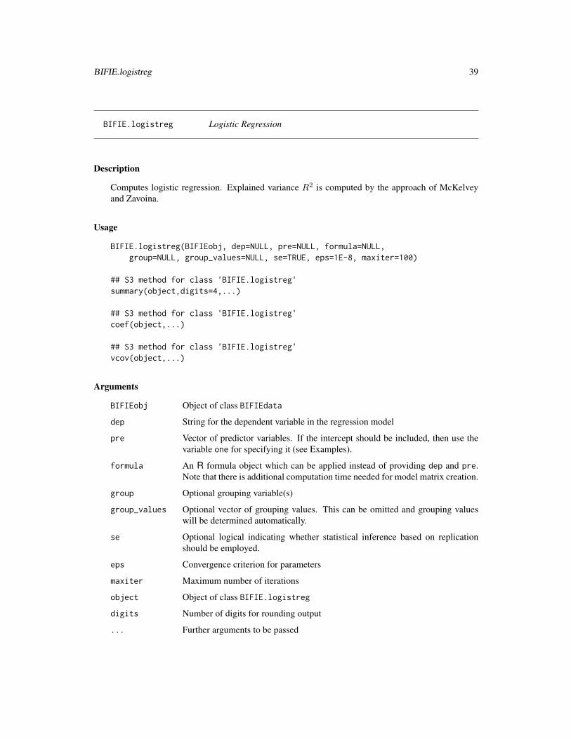
BIFIE.logistreg Logistic Regression
Description
Computes logistic regression. Explained variance R2 is computed by the approach of McKelveyand Zavoina.
Usage
BIFIE.logistreg(BIFIEobj, dep=NULL, pre=NULL, formula=NULL,group=NULL, group_values=NULL, se=TRUE, eps=1E-8, maxiter=100)
## S3 method for class 'BIFIE.logistreg'summary(object,digits=4,...)
## S3 method for class 'BIFIE.logistreg'coef(object,...)
## S3 method for class 'BIFIE.logistreg'vcov(object,...)
Arguments
BIFIEobj Object of class BIFIEdata
dep String for the dependent variable in the regression model
pre Vector of predictor variables. If the intercept should be included, then use thevariable one for specifying it (see Examples).
formula An R formula object which can be applied instead of providing dep and pre.Note that there is additional computation time needed for model matrix creation.
group Optional grouping variable(s)
group_values Optional vector of grouping values. This can be omitted and grouping valueswill be determined automatically.
se Optional logical indicating whether statistical inference based on replicationshould be employed.
eps Convergence criterion for parameters
maxiter Maximum number of iterations
object Object of class BIFIE.logistreg
digits Number of digits for rounding output
... Further arguments to be passed
40 BIFIE.logistreg
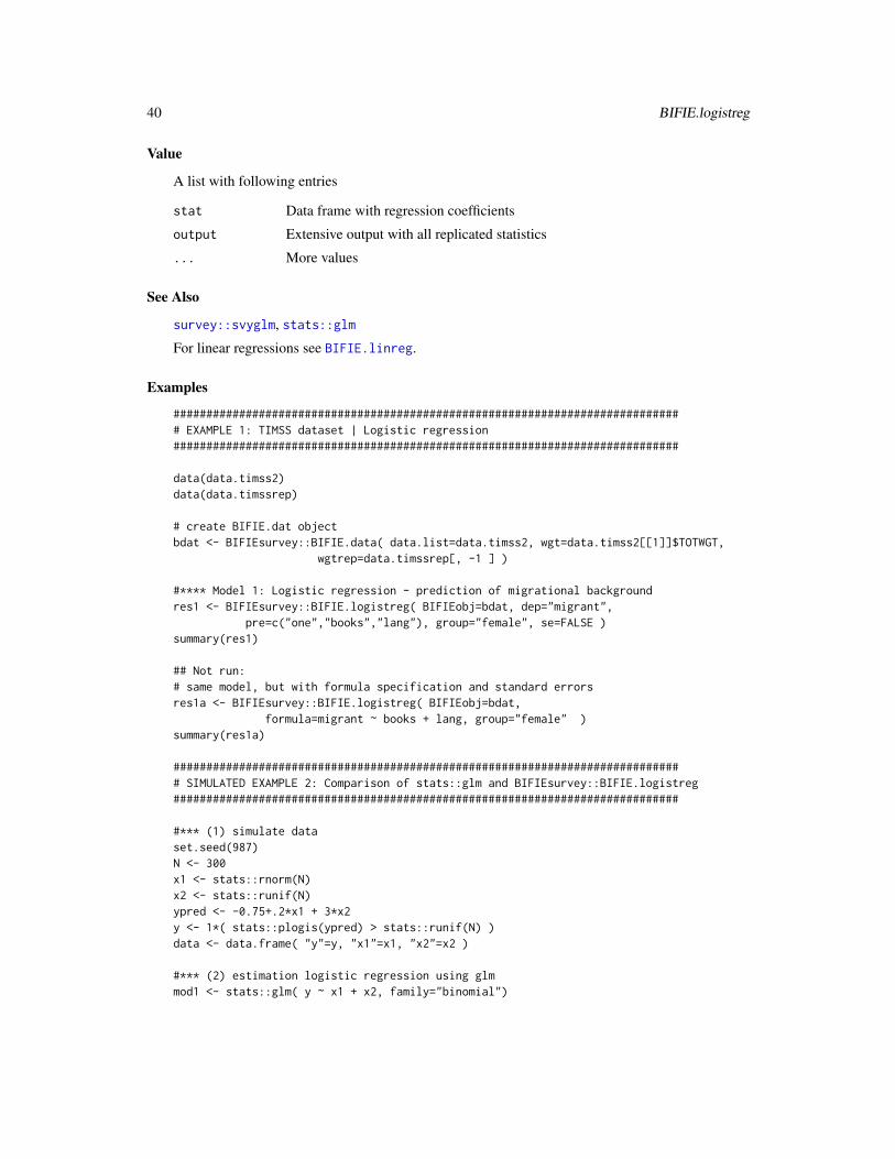
Value
A list with following entries
stat Data frame with regression coefficients
output Extensive output with all replicated statistics
... More values
See Also
survey::svyglm, stats::glm
For linear regressions see BIFIE.linreg.
Examples
############################################################################## EXAMPLE 1: TIMSS dataset | Logistic regression#############################################################################
data(data.timss2)data(data.timssrep)
# create BIFIE.dat objectbdat <- BIFIEsurvey::BIFIE.data( data.list=data.timss2, wgt=data.timss2[[1]]$TOTWGT,
wgtrep=data.timssrep[, -1 ] )
#**** Model 1: Logistic regression - prediction of migrational backgroundres1 <- BIFIEsurvey::BIFIE.logistreg( BIFIEobj=bdat, dep="migrant",
pre=c("one","books","lang"), group="female", se=FALSE )summary(res1)
## Not run:# same model, but with formula specification and standard errorsres1a <- BIFIEsurvey::BIFIE.logistreg( BIFIEobj=bdat,
formula=migrant ~ books + lang, group="female" )summary(res1a)
############################################################################## SIMULATED EXAMPLE 2: Comparison of stats::glm and BIFIEsurvey::BIFIE.logistreg#############################################################################
#*** (1) simulate dataset.seed(987)N <- 300x1 <- stats::rnorm(N)x2 <- stats::runif(N)ypred <- -0.75+.2*x1 + 3*x2y <- 1*( stats::plogis(ypred) > stats::runif(N) )data <- data.frame( "y"=y, "x1"=x1, "x2"=x2 )
#*** (2) estimation logistic regression using glmmod1 <- stats::glm( y ~ x1 + x2, family="binomial")
BIFIE.mva 41
#*** (3) estimation logistic regression using BIFIEdata# create BIFIEdata object by defining 30 Jackknife zonesbifiedata <- BIFIEsurvey::BIFIE.data.jack( data, jktype="JK_RANDOM", ngr=30 )summary(bifiedata)# estimate logistic regressionmod2 <- BIFIEsurvey::BIFIE.logistreg( bifiedata, formula=y ~ x1+x2 )
#*** (4) compare resultssummary(mod2) # BIFIE.logistregsummary(mod1) # glm
## End(Not run)
BIFIE.mva Missing Value Analysis
Description
Conducts a missing value analysis.
Usage
BIFIE.mva( BIFIEobj, missvars, covariates=NULL, se=TRUE )
## S3 method for class 'BIFIE.mva'summary(object,digits=4,...)
Arguments
BIFIEobj Object of class BIFIEdata
missvars Vector of variables for which missing value statistics should be computed
covariates Vector of variables which work as covariates
se Optional logical indicating whether statistical inference based on replicationshould be employed.
object Object of class BIFIE.correl
digits Number of digits for rounding output
... Further arguments to be passed
Value
A list with following entries
stat.mva Data frame with missing value statistics
res_list List with extensive output split according to each variable in missvars
... More values
42 BIFIE.pathmodel
Examples
############################################################################## EXAMPLE 1: Imputed TIMSS dataset#############################################################################
data(data.timss1)data(data.timssrep)
# create BIFIE.dat objectBIFIEdata <- BIFIEsurvey::BIFIE.data( data.list=data.timss1,
wgt=data.timss1[[1]]$TOTWGT, wgtrep=data.timssrep[, -1 ] )
# missing value analysis for "scsci" and "books" and three covariatesres1 <- BIFIEsurvey::BIFIE.mva( BIFIEdata, missvars=c("scsci", "books" ),
covariates=c("ASMMAT", "female", "ASSSCI") )summary(res1)
# missing value analysis without statistical inference and without covariatesres2 <- BIFIEsurvey::BIFIE.mva( BIFIEdata, missvars=c("scsci", "books"), se=FALSE)summary(res2)
BIFIE.pathmodel Path Model Estimation
Description
This function computes a path model. Predictors are allowed to possess measurement errors.Known measurement error variances (and covariances) or reliabilities can be specified by the user.Alternatively, a set of indicators can be defined for each latent variable, and for each imputed andreplicated dataset the measurement error variance is determined by means of calculating the reli-ability Cronbachs alpha. Measurement errors are handled by adjusting covariance matrices (seeBuonaccorsi, 2010, Ch. 5).
Usage
BIFIE.pathmodel( BIFIEobj, lavaan.model, reliability=NULL, group=NULL,group_values=NULL, se=TRUE )
## S3 method for class 'BIFIE.pathmodel'summary(object,digits=4,...)
## S3 method for class 'BIFIE.pathmodel'coef(object,...)
## S3 method for class 'BIFIE.pathmodel'vcov(object,...)
BIFIE.pathmodel 43
Arguments
BIFIEobj Object of class BIFIEdata
lavaan.model String including the model specification in lavaan syntax. lavaan.model alsoallows the extended functionality in the TAM::lavaanify.IRT function.
reliability Optional vector containing the reliabilities of each variable. This vector can alsoinclude only a subset of all variables.
group Optional grouping variable(s)
group_values Optional vector of grouping values. This can be omitted and grouping valueswill be determined automatically.
se Optional logical indicating whether statistical inference based on replicationshould be employed.
object Object of class BIFIE.pathmodel
digits Number of digits for rounding output
... Further arguments to be passed
Details
The following conventions are used as parameter labels in the output.
Y~X is the regression coefficient of the regression from Y on X .
X->Z->Y denotes the path coefficient from X to Y passing the mediating variable Z.
X-+>Y denotes the total effect (of all paths) from X to Y .
X-~>Y denotes the sum of all indirect effects from X to Y .
The parameter suffix _stand refers to parameters for which all variables are standardized.
Value
A list with following entries
stat Data frame with unstandardized and standardized regression coefficients, pathcoefficients, total and indirect effects, residual variances, and R2
output Extensive output with all replicated statistics
... More values
References
Buonaccorsi, J. P. (2010). Measurement error: Models, methods, and applications. CRC Press.
See Also
See the lavaan and lavaan.survey package.
For the lavaan syntax, see lavaan::lavaanify and TAM::lavaanify.IRT
44 BIFIE.twolevelreg
Examples
## Not run:############################################################################## EXAMPLE 1: Path model data.bifie01#############################################################################
data(data.bifie01)dat <- data.bifie01# create dataset with replicate weights and plausible valuesbifieobj <- BIFIEsurvey::BIFIE.data.jack( data=dat, jktype="JK_TIMSS",
jkzone="JKCZONE", jkrep="JKCREP", wgt="TOTWGT",pv_vars=c("ASMMAT","ASSSCI") )
#**************************************************************#*** Model 1: Path modellavmodel1 <- "
ASMMAT ~ ASBG07A + ASBG07B + ASBM03 + ASBM02A + ASBM02E# define latent variable with 2nd and 3rd item in reversed scoringASBM03=~ 1*ASBM03A + (-1)*ASBM03B + (-1)*ASBM03C + 1*ASBM03DASBG07A ~ ASBM02EASBG07A ~~ .2*ASBG07A # measurement error variance of .20ASBM02E ~~ .45*ASBM02E # measurement error variance of .45ASBM02E ~ ASBM02A + ASBM02B
"#--- Model 1a: model calculated by gendermod1a <- BIFIEsurvey::BIFIE.pathmodel( bifieobj, lavmodel1, group="female" )summary(mod1a)
#--- Model 1b: Input of some known reliabilitiesreliability <- c( "ASBM02B"=.6, "ASBM02A"=.8 )mod1b <- BIFIEsurvey::BIFIE.pathmodel( bifieobj, lavmodel1, reliability=reliability)summary(mod1b)
#**************************************************************#*** Model 2: Linear regression with errors in predictors
# specify lavaan modellavmodel2 <- "
ASMMAT ~ ASBG07A + ASBG07B + ASBM03AASBG07A ~~ .2*ASBG07A
"mod2 <- BIFIEsurvey::BIFIE.pathmodel( bifieobj, lavmodel2 )summary(mod2)
## End(Not run)
BIFIE.twolevelreg Two Level Regression
BIFIE.twolevelreg 45
Description
This function computes the hierarchical two level model with random intercepts and random slopes.The full maximum likelihood estimation is conducted by means of an EM algorithm (Raudenbush& Bryk, 2002).
Usage
BIFIE.twolevelreg( BIFIEobj, dep, formula.fixed, formula.random, idcluster,wgtlevel2=NULL, wgtlevel1=NULL, group=NULL, group_values=NULL,recov_constraint=NULL, se=TRUE, globconv=1E-6, maxiter=1000 )
## S3 method for class 'BIFIE.twolevelreg'summary(object,digits=4,...)
## S3 method for class 'BIFIE.twolevelreg'coef(object,...)
## S3 method for class 'BIFIE.twolevelreg'vcov(object,...)
Arguments
BIFIEobj Object of class BIFIEdata
dep String for the dependent variable in the regression model
formula.fixed An R formula for fixed effects
formula.random An R formula for random effects
idcluster Cluster identifier. The cluster identifiers must be sorted in the BIFIE.data ob-ject.
wgtlevel2 Name of Level 2 weight variable
wgtlevel1 Name of Level 1 weight variable. This is optional. If it is not provided, wgtlevelis calculated from the total weight and wgtlevel2.
group Optional grouping variable
group_values Optional vector of grouping values. This can be omitted and grouping valueswill be determined automatically.
recov_constraint
Matrix for constraints of random effects covariance matrix. The random effectsare numbered according to the order in the specification in formula.random.The first column in recov_constraint contains the row index in the covariancematrix, the second column the column index and the third column the value tobe fixed.
se Optional logical indicating whether statistical inference based on replicationshould be employed. In case of se=FALSE, standard errors are computed as max-imum likelihood estimates under the assumption of random sampling of level 2clusters.
globconv Convergence criterion for maximum parameter change
46 BIFIE.twolevelreg
maxiter Maximum number of iterations
object Object of class BIFIE.twolevelreg
digits Number of digits for rounding output
... Further arguments to be passed
Details
The implemented random slope model can be written as
yij =Xijγ +Zijuj + εij
where yij is the dependent variable,Xij includes the fixed effects predictors (specified by formula.fixed)andZij includes the random effects predictors (specified by formula.random). The random effectsuj follow a multivariate normal distribution.
The function also computes a variance decomposition of explained variance due to fixed and randomeffects for the within and the between level. This variance decomposition is conducted for thepredictor matrices X and Z. It is assumed that Xij = XB
j + XWij . The different sources of
variance are computed by formulas as proposed in Snijders and Bosker (2012, Ch. 7).
Value
A list with following entries
stat Data frame with coefficients and different sources of variance.
output Extensive output with all replicated statistics
... More values
References
Raudenbush, S. W., & Bryk, A. S. (2002). Hierarchical linear models: Applications and dataanalysis methods. Thousand Oaks: Sage.
Snijders, T. A. B., & Bosker, R. J. (2012). Multilevel analysis: An introduction to basic and ad-vanced multilevel modeling. Thousand Oaks: Sage.
See Also
The lme4::lmer function in the lme4 package allows only weights at the first level.
See the WeMix package (and the function WeMix::mix) for estimation of mixed effects modelswith weights at different levels.
Examples
## Not run:library(lme4)
############################################################################## EXAMPLE 1: Dataset data.bifie01 | TIMSS 2011#############################################################################
BIFIE.twolevelreg 47
data(data.bifie01)dat <- data.bifie01set.seed(987)
# create dataset with replicate weights and plausible valuesbdat1 <- BIFIEsurvey::BIFIE.data.jack( data=dat, jktype="JK_TIMSS", jkzone="JKCZONE",
jkrep="JKCREP", wgt="TOTWGT", pv_vars=c("ASMMAT","ASSSCI") )
# create dataset without plausible values and ignoring weightsbdat2 <- BIFIEsurvey::BIFIE.data.jack( data=dat, jktype="JK_RANDOM", ngr=10 )#=> standard errors from ML estimation
#***********************************************# Model 1: Random intercept model
#--- Model 1a: without weights, first plausible valuemod1a <- BIFIEsurvey::BIFIE.twolevelreg( BIFIEobj=bdat2, dep="ASMMAT01",
formula.fixed=~ 1, formula.random=~ 1, idcluster="idschool",wgtlevel2="one", se=FALSE )
summary(mod1a)
#--- Model 1b: estimation in lme4mod1b <- lme4::lmer( ASMMAT01 ~ 1 + ( 1 | idschool), data=dat, REML=FALSE)summary(mod1b)
#--- Model 1c: Like Model 1a but for five plausible values and ML inferencemod1c <- BIFIEsurvey::BIFIE.twolevelreg( BIFIEobj=bdat1, dep="ASMMAT",
formula.fixed=~ 1, formula.random=~ 1, idcluster="idschool",wgtlevel2="one", se=FALSE )
summary(mod1c)
#--- Model 1d: weights and sampling design and all plausible valuesmod1d <- BIFIEsurvey::BIFIE.twolevelreg( BIFIEobj=bdat1, dep="ASMMAT",
formula.fixed=~ 1, formula.random=~ 1, idcluster="idschool",wgtlevel2="SCHWGT" )
summary(mod1d)
#***********************************************# Model 2: Random slope model
#--- Model 2a: without weightsmod2a <- BIFIEsurvey::BIFIE.twolevelreg( BIFIEobj=bdat2, dep="ASMMAT01",
formula.fixed=~ female + ASBG06A, formula.random=~ ASBG06A,idcluster="idschool", wgtlevel2="one", se=FALSE )
summary(mod2a)
#--- Model 2b: estimation in lme4mod2b <- lme4::lmer( ASMMAT01 ~ female + ASBG06A + ( 1 + ASBG06A | idschool),
data=dat, REML=FALSE)summary(mod2b)
#--- Model 2c: weights and sampling design and all plausible values
48 BIFIE.twolevelreg
mod2c <- BIFIEsurvey::BIFIE.twolevelreg( BIFIEobj=bdat1, dep="ASMMAT",formula.fixed=~ female + ASBG06A, formula.random=~ ASBG06A,idcluster="idschool", wgtlevel2="SCHWGT", maxiter=500, se=FALSE)
summary(mod2c)
#--- Model 2d: Uncorrelated intecepts and slopes
# constraint for zero covariance between intercept and sloperecov_constraint <- matrix( c(1,2,0), ncol=3 )mod2d <- BIFIEsurvey::BIFIE.twolevelreg( BIFIEobj=bdat2, dep="ASMMAT01",
formula.fixed=~ female + ASBG06A, formula.random=~ ASBG06A,idcluster="idschool", wgtlevel2="one", se=FALSE,recov_constraint=recov_constraint )
summary(mod2d)
#--- Model 2e: Fixed entries in the random effects covariance matrix
# two constraints for random effects covariance# Cov(Int, Slo)=0 # zero slope for intercept and slope# Var(Slo)=10 # slope variance of 10recov_constraint <- matrix( c(1,2,0,
2,2,10), ncol=3, byrow=TRUE)mod2e <- BIFIEsurvey::BIFIE.twolevelreg( BIFIEobj=bdat2, dep="ASMMAT01",
formula.fixed=~ female + ASBG06A, formula.random=~ ASBG06A,idcluster="idschool", wgtlevel2="one", se=FALSE,recov_constraint=recov_constraint )
summary(mod2e)
############################################################################## SIMULATED EXAMPLE 2: Two-level regression with random slopes#############################################################################
#--- (1) simulate dataset.seed(9876)NC <- 100 # number of clustersNj <- 20 # number of persons per clustericcx <- .4 # intra-class correlation predictortheta <- c( 0.7, .3 ) # fixed effectsTmat <- diag( c(.3, .1 ) ) # variances of random intercept and slopesig2 <- .60 # residual varianceN <- NC*Njidcluster <- rep( 1:NC, each=Nj )dat1 <- data.frame("idcluster"=idcluster )dat1$X <- rep( stats::rnorm( NC, sd=sqrt(iccx) ), each=Nj ) +
stats::rnorm( N, sd=sqrt( 1 - iccx) )dat1$Y <- theta[1] + rep( stats::rnorm(NC, sd=sqrt(Tmat[1,1] ) ), each=Nj ) +
theta[2] + rep( stats::rnorm(NC, sd=sqrt(Tmat[2,2])), each=Nj )) * dat1$X +stats::rnorm(N, sd=sqrt(sig2) )
#--- (2) create design objectbdat1 <- BIFIEsurvey::BIFIE.data.jack( data=dat1, jktype="JK_GROUP", jkzone="idcluster")summary(bdat1)
BIFIE.univar 49
#*** Model 1: Random slope model (ML standard errors)
#- estimation using BIFIE.twolevelregmod1a <- BIFIEsurvey::BIFIE.twolevelreg( BIFIEobj=bdat1, dep="Y",
formula.fixed=~ 1+X, formula.random=~ 1+X, idcluster="idcluster",wgtlevel2="one", se=FALSE )
summary(mod1a)
#- estimation in lme4mod1b <- lme4::lmer( Y ~ X + ( 1+X | idcluster), data=dat1, REML=FALSE )summary(mod1b)
#- using Jackknife for inferencemod1c <- BIFIEsurvey::BIFIE.twolevelreg( BIFIEobj=bdat1, dep="Y",
formula.fixed=~ 1+X, formula.random=~ 1+X, idcluster="idcluster",wgtlevel2="one", se=TRUE )
summary(mod1c)
# extract coefficientscoef(mod1a)coef(mod1c)# covariance matrixvcov(mod1a)vcov(mod1c)
## End(Not run)
BIFIE.univar Univariate Descriptive Statistics (Means and Standard Deviations)
Description
Computes some univariate descriptive statistics (means and standard deviations).
Usage
BIFIE.univar(BIFIEobj, vars, group=NULL, group_values=NULL, se=TRUE)
## S3 method for class 'BIFIE.univar'summary(object,digits=3,...)
## S3 method for class 'BIFIE.univar'coef(object,...)
## S3 method for class 'BIFIE.univar'vcov(object,...)
50 BIFIE.univar
Arguments
BIFIEobj Object of class BIFIEdata
vars Vector of variables for which statistics should be computed
group Optional grouping variable(s)
group_values Optional vector of grouping values. This can be omitted and grouping valueswill be determined automatically.
se Optional logical indicating whether statistical inference based on replicationshould be employed.
object Object of class BIFIE.univar
digits Number of digits for rounding output
... Further arguments to be passed
Value
A list with following entries
stat Data frame with univariate statistics
stat_M Data frame with means
stat_SD Data frame with standard deviations
output Extensive output with all replicated statistics
... More values
See Also
See BIFIE.univar.test for a test of equal means and effect sizes η and d.
Descriptive statistics without statistical inference can be estimated by the collection of miceadds::ma.wtd.statNAfunctions from the miceadds package.
Further descriptive functions:
survey::svymean, intsvy::timss.mean, intsvy::timss.mean.pv, stats::weighted.mean, Hmisc::wtd.mean,miceadds::ma.wtd.meanNA
survey::svyvar, Hmisc::wtd.var, miceadds::ma.wtd.sdNA, miceadds::ma.wtd.covNA
Examples
############################################################################## EXAMPLE 1: Imputed TIMSS dataset#############################################################################
data(data.timss1)data(data.timssrep)
# create BIFIE.dat objectbdat <- BIFIEsurvey::BIFIE.data( data.list=data.timss1, wgt=data.timss1[[1]]$TOTWGT,
wgtrep=data.timssrep[, -1 ] )
BIFIE.univar.test 51
# compute descriptives for plausible valuesres1 <- BIFIEsurvey::BIFIE.univar( bdat, vars=c("ASMMAT","ASSSCI","books") )summary(res1)
# split descriptives by number of booksres2 <- BIFIEsurvey::BIFIE.univar( bdat, vars=c("ASMMAT","ASSSCI"), group="books",
group_values=1:5)summary(res2)
############################################################################## EXAMPLE 2: TIMSS dataset with missings#############################################################################
data(data.timss2)data(data.timssrep)
# use first dataset with missing data from data.timss2bdat1 <- BIFIEsurvey::BIFIE.data( data.list=data.timss2[[1]], wgt=data.timss2[[1]]$TOTWGT,
wgtrep=data.timssrep[, -1 ])
# some descriptive statistics without statistical inferenceres1a <- BIFIEsurvey::BIFIE.univar( bdat1, vars=c("ASMMAT","ASSSCI","books"), se=FALSE)# descriptive statistics with statistical inferenceres1b <- BIFIEsurvey::BIFIE.univar( bdat1, vars=c("ASMMAT","ASSSCI","books") )summary(res1a)summary(res1b)
# split descriptives by number of booksres2 <- BIFIEsurvey::BIFIE.univar( bdat1, vars=c("ASMMAT","ASSSCI"), group="books")# Note that if group_values is not specified as an argument it will be# automatically determined by the observed frequencies in the datasetsummary(res2)
BIFIE.univar.test Analysis of Variance and Effect Sizes for Univariate Statistics
Description
Computes a Wald test which tests equality of means (univariate analysis of variance). In addition,the d and η effect sizes are computed.
Usage
BIFIE.univar.test(BIFIE.method, wald_test=TRUE)
## S3 method for class 'BIFIE.univar.test'summary(object,digits=4,...)
52 BIFIE.univar.test
Arguments
BIFIE.method Object of class BIFIE.univar
wald_test Optional logical indicating whether a Wald test should be performed.
object Object of class BIFIE.univar.test
digits Number of digits for rounding output
... Further arguments to be passed
Value
A list with following entries
stat.F Data frame with F statistic for Wald test
stat.eta Data frame with η effect size and its inference
stat.dstat Data frame with Cohen’s d effect size and its inference
... More values
See Also
BIFIE.univar
Examples
############################################################################## EXAMPLE 1: Imputed TIMSS dataset - One grouping variable#############################################################################
data(data.timss1)data(data.timssrep)
# create BIFIE.dat objectbdat <- BIFIEsurvey::BIFIE.data( data.list=data.timss1, wgt=data.timss1[[1]]$TOTWGT,
wgtrep=data.timssrep[, -1 ] )
#**** Model 1: 3 variables splitted by bookres1 <- BIFIEsurvey::BIFIE.univar( bdat, vars=c("ASMMAT", "ASSSCI","scsci"),
group="books")summary(res1)# analysis of variancetres1 <- BIFIEsurvey::BIFIE.univar.test(res1)summary(tres1)
#**** Model 2: One variable splitted by genderres2 <- BIFIEsurvey::BIFIE.univar( bdat, vars=c("ASMMAT"), group="female" )summary(res2)# analysis of variancetres2 <- BIFIEsurvey::BIFIE.univar.test(res2)summary(tres2)
## Not run:
BIFIE.waldtest 53
#**** Model 3: Univariate statistic: mathres3 <- BIFIEsurvey::BIFIE.univar( bdat, vars=c("ASMMAT") )summary(res3)tres3 <- BIFIEsurvey::BIFIE.univar.test(res3)
############################################################################## EXAMPLE 2: Imputed TIMSS dataset - Two grouping variables#############################################################################
data(data.timss1)data(data.timssrep)
# create BIFIE.dat objectbdat <- BIFIEsurvey::BIFIE.data( data.list=data.timss1, wgt=data.timss1[[1]]$TOTWGT,
wgtrep=data.timssrep[, -1 ] )
#**** Model 1: 3 variables splitted by book and femaleres1 <- BIFIEsurvey::BIFIE.univar(bdat, vars=c("ASMMAT", "ASSSCI","scsci"),
group=c("books","female"))summary(res1)
# analysis of variancetres1 <- BIFIEsurvey::BIFIE.univar.test(res1)summary(tres1)
# extract data frame with Cohens d statisticdstat <- tres1$stat.dstat
# extract d values for gender comparisons with same value of books# -> 'books' refers to the first variableind <- which(
unlist( lapply( strsplit( dstat$groupval1, "#"), FUN=function(vv){vv[1]}) )==unlist( lapply( strsplit( dstat$groupval2, "#"), FUN=function(vv){vv[1]}) )
)dstat[ ind, ]
## End(Not run)
BIFIE.waldtest Wald Tests for BIFIE Methods
Description
This function performs a Wald test for objects of classes BIFIE.by, BIFIE.correl, BIFIE.crosstab,BIFIE.freq, BIFIE.linreg, BIFIE.logistreg and BIFIE.univar.
Usage
BIFIE.waldtest(BIFIE.method, Cdes, rdes, type=NULL)
54 BIFIE.waldtest
## S3 method for class 'BIFIE.waldtest'summary(object,digits=4,...)
Arguments
BIFIE.method Object of classes BIFIE.by, BIFIE.correl, BIFIE.crosstab, BIFIE.freq,BIFIE.linreg, BIFIE.logistreg or BIFIE.univar (see parnames in the Out-put of these methods for saved parameters)
Cdes Design matrix C (see Details)
rdes Design vector r (see Details)
type Only applies to BIFIE.correl. In case of type="cov" covariances instead ofcorrelations are used for parameter tests.
object Object of class BIFIE.waldtest
digits Number of digits for rounding output
... Further arguments to be passed
Details
The Wald test is conducted for a parameter vector θ, specifying the hypothesis Cθ = r. Statisticalinference is performed by using the D1 and the D2 statistic (Enders, 2010, Ch. 8).
For objects of class bifie.univar, only hypotheses with respect to means are implemented.
Value
A list with following entries
stat.D Data frame with D1 and D2 statistic, degrees of freedom and p value
... More values
References
Enders, C. K. (2010). Applied missing data analysis. Guilford Press.
See Also
survey::regTermTest, survey::anova.svyglm, car::linearHypothesis
Examples
############################################################################## EXAMPLE 1: Imputed TIMSS dataset#############################################################################
data(data.timss1)data(data.timssrep)
# create BIFIE.dat objectbdat <- BIFIEsurvey::BIFIE.data( data.list=data.timss1, wgt=data.timss1[[1]]$TOTWGT,
BIFIE.waldtest 55
wgtrep=data.timssrep[, -1 ] )
#******************#*** Model 1: Linear regressionres1 <- BIFIEsurvey::BIFIE.linreg( bdat, dep="ASMMAT", pre=c("one","books","migrant"),
group="female" )summary(res1)
#*** Wald test which tests whether sigma and R^2 values are the sameres1$parnames # parameter namespn <- res1$parnames ; PN <- length(pn)Cdes <- matrix(0,nrow=2, ncol=PN)colnames(Cdes) <- pn# equality of R^2 ( R^2(female0) - R^2(female1)=0 )Cdes[ 1, c("R^2_NA_female_0", "R^2_NA_female_1" ) ] <- c(1,-1)# equality of sigma ( sigma(female0) - sigma(female1)=0)Cdes[ 2, c("sigma_NA_female_0", "sigma_NA_female_1" ) ] <- c(1,-1)# design vectorrdes <- rep(0,2)# perform Wald testwmod1 <- BIFIEsurvey::BIFIE.waldtest( BIFIE.method=res1, Cdes=Cdes, rdes=rdes )summary(wmod1)
## Not run:#******************#*** Model 2: Correlations
# compute some correlationsres2a <- BIFIEsurvey::BIFIE.correl( bdat, vars=c("ASMMAT","ASSSCI","migrant","books"))summary(res2a)
# test whether r(MAT,migr)=r(SCI,migr) and r(MAT,books)=r(SCI,books)pn <- res2a$parnames; PN <- length(pn)Cdes <- matrix( 0, nrow=2, ncol=PN )colnames(Cdes) <- pnCdes[ 1, c("ASMMAT_migrant", "ASSSCI_migrant") ] <- c(1,-1)Cdes[ 2, c("ASMMAT_books", "ASSSCI_books") ] <- c(1,-1)rdes <- rep(0,2)# perform Wald testwres2a <- BIFIEsurvey::BIFIE.waldtest( res2a, Cdes, rdes )summary(wres2a)
#******************#*** Model 3: Frequencies
# Number of books splitted by genderres3a <- BIFIEsurvey::BIFIE.freq( bdat, vars=c("books"), group="female" )summary(res3a)
# test whether book(cat4,female0)+book(cat5,female0)=book(cat4,female1)+book(cat5,female5)pn <- res3a$parnamesPN <- length(pn)Cdes <- matrix( 0, nrow=1, ncol=PN )
56 BIFIEdata.select
colnames(Cdes) <- pnCdes[ 1, c("books_4_female_0", "books_5_female_0",
"books_4_female_1", "books_5_female_1" ) ] <- c(1,1,-1,-1)rdes <- c(0)# Wald testwres3a <- BIFIEsurvey::BIFIE.waldtest( res3a, Cdes, rdes )summary(wres3a)
#******************#*** Model 4: Means
# math and science score splitted by genderres4a <- BIFIEsurvey::BIFIE.univar( bdat, vars=c("ASMMAT","ASSSCI"), group="female")summary(res4a)
# test whether there are significant gender differences in math and science#=> multivariate ANOVApn <- res4a$parnamesPN <- length(pn)Cdes <- matrix( 0, nrow=2, ncol=PN )colnames(Cdes) <- pnCdes[ 1, c("ASMMAT_female_0", "ASMMAT_female_1" ) ] <- c(1,-1)Cdes[ 2, c("ASSSCI_female_0", "ASSSCI_female_1" ) ] <- c(1,-1)rdes <- rep(0,2)# Wald testwres4a <- BIFIEsurvey::BIFIE.waldtest( res4a, Cdes, rdes )summary(wres4a)
## End(Not run)
BIFIEdata.select Selection of Variables and Imputed Datasets for Objects of ClassBIFIEdata
Description
This function select variables and some (or all) imputed datasets of an object of class BIFIEdataand saves the resulting object also of class BIFIEdata.
Usage
BIFIEdata.select(bifieobj, varnames=NULL, impdata.index=NULL)
Arguments
bifieobj Object of class BIFIEdata
varnames Variables chosen for the selection
impdata.index Selected indices of imputed datasets
BIFIEdata2svrepdesign 57
Value
An object of class BIFIEdata saved in a non-compact or compact way, see value cdata
See Also
See BIFIE.data for creating BIFIEdata objects.
Examples
############################################################################## EXAMPLE 1: Some manipulations of BIFIEdata objects created from data.timss1#############################################################################data(data.timss1)data(data.timssrep)
# create BIFIEdatabdat1 <- BIFIEsurvey::BIFIE.data( data.list=data.timss1, wgt=data.timss1[[1]]$TOTWGT,
wgtrep=data.timssrep[, -1 ])summary(bdat1)
# create BIFIEcdata objectbdat2 <- BIFIEsurvey::BIFIE.data( data.list=data.timss1, wgt=data.timss1[[1]]$TOTWGT,
wgtrep=data.timssrep[, -1 ], cdata=TRUE )summary(bdat2)
# selection of variables for BIFIEdata objectbdat1a <- BIFIEsurvey::BIFIEdata.select( bdat1, varnames=bdat1$varnames[ 1:7 ] )# selection of variables and 1st, 2nd and 4th imputed datasets of BIFIEcdata objectbdat2a <- BIFIEsurvey::BIFIEdata.select( bdat2, varnames=bdat2$varnames[ 1:7 ],
impdata.index=c(1,2,4) )summary(bdat1a)summary(bdat2a)
BIFIEdata2svrepdesign Conversion of a BIFIEdata Object into a svyrep Object in the surveyPackage (and the other way around)
Description
The function BIFIEdata2svrepdesign converts of a BIFIEdata object into a svyrep object in thesurvey package.
The function svrepdesign2BIFIEdata converts a svyrep object in the survey package into anobject of class BIFIEdata.
Usage
BIFIEdata2svrepdesign(bifieobj, varnames=NULL, impdata.index=NULL)
svrepdesign2BIFIEdata(svrepdesign, varnames=NULL, cdata=FALSE)
58 BIFIEdata2svrepdesign
Arguments
bifieobj Object of class BIFIEdata
varnames Optional vector with variable names
impdata.index Selected indices of imputed datasets
svrepdesign Object of class svyrep.design or svyimputationList
cdata Logical inducating whether BIFIEdata object should be saved in compact for-mat
Value
Function BIFIEdata2svrepdesign: Object of class svyrep.design or svyimputationList
Function svrepdesign2BIFIEdata: Object of class BIFIEdata
See Also
See the BIFIE.data function for creating objects of class BIFIEdata in BIFIEsurvey.
See the survey::svrepdesign function in the survey package.
Examples
## Not run:############################################################################## EXAMPLE 1: One dataset, TIMSS replication design#############################################################################
data(data.timss3)data(data.timssrep)
#--- create BIFIEdata objectbdat3 <- BIFIEsurvey::BIFIE.data.jack(data.timss3, jktype="JK_TIMSS")summary(bdat3)
#--- create survey object directly in survey packagedat3a <- as.data.frame( cbind( data.timss3, data.timssrep ) )RR <- ncol(data.timssrep) - 1 # number of jackknife zonessvydes3a <- survey::svrepdesign(data=dat3a, weights=~TOTWGT,type="JKn",
repweights='w_fstr[0-9]', scale=1, rscales=rep(1,RR), mse=TRUE )print(svydes3a)
#--- create survey object by converting the BIFIEdata object to surveysvydes3b <- BIFIEsurvey::BIFIEdata2svrepdesign(bdat3)
#--- convert survey object into BIFIEdata objectbdat3e <- BIFIEsurvey::svrepdesign2BIFIEdata(svrepdesign=svydes3b)
#*** compare results for the mean in Mathematics scoresmod1a <- BIFIEsurvey::BIFIE.univar( bdat3, vars="ASMMAT1")mod1b <- survey::svymean( ~ ASMMAT1, design=svydes3a )
BIFIEsurvey-utilities 59
mod1c <- survey::svymean( ~ ASMMAT1, design=svydes3b )lavmodel <- "ASMMAT1 ~ 1"mod1d <- BIFIEsurvey::BIFIE.lavaan.survey(lavmodel, svyrepdes=svydes3b)
#- coefficientscoef(mod1a); coef(mod1b); coef(mod1c); coef(mod1d)[1]#- standard errorssurvey::SE(mod1a); survey::SE(mod1b); survey::SE(mod1c); sqrt(vcov(mod1d)[1,1])
############################################################################## EXAMPLE 2: Multiply imputed datasets, TIMSS replication design#############################################################################
data(data.timss2)data(data.timssrep)
#--- create BIFIEdata objectbdat4 <- BIFIEsurvey::BIFIE.data( data=data.timss2, wgt="TOTWGT",
wgtrep=data.timssrep[,-1], fayfac=1)print(bdat4)
#--- create object with imputed datasets in surveydatL <- mitools::imputationList( data.timss2 )RR <- ncol(data.timssrep) - 1weights <- data.timss2[[1]]$TOTWGTrepweights <- data.timssrep[,-1]svydes4a <- survey::svrepdesign(data=datL, weights=weights, type="other",
repweights=repweights, scale=1, rscales=rep(1,RR), mse=TRUE)print(svydes4a)
#--- create BIFIEdata object with conversion functionsvydes4b <- BIFIEsurvey::BIFIEdata2svrepdesign(bdat4)
#--- reconvert survey object into BIFIEdata objectbdat4c <- BIFIEsurvey::svrepdesign2BIFIEdata(svrepdesign=svydes4b)
#*** compare results for a meanmod1a <- BIFIEsurvey::BIFIE.univar(bdat4, vars="ASMMAT")mod1b <- mitools::MIcombine( with(svydes4a, survey::svymean( ~ ASMMAT, design=svydes4a )))mod1c <- mitools::MIcombine( with(svydes4b, survey::svymean( ~ ASMMAT, design=svydes4b )))
# resultscoef(mod1a); coef(mod1b); coef(mod1c)survey::SE(mod1a); survey::SE(mod1b); survey::SE(mod1c)
## End(Not run)
BIFIEsurvey-utilities Utility Functions in BIFIEsurvey
60 bifietable
Description
Utility functions in BIFIEsurvey.
Usage
## Rubin rules for combining multiple imputation estimatesbifiesurvey_rcpp_rubin_rules(estimates, variances)
## computation of replication variancebifiesurvey_rcpp_replication_variance(pars, pars_repl, fay_factor)
## statistical inference for nested multiple imputationBIFIE_NMI_inference_parameters( parsM, parsrepM, fayfac, RR, Nimp, Nimp_NMI,
comp_cov=FALSE)
Arguments
estimates Vector
variances Vector
pars Matrix
pars_repl Matrix
fay_factor Vector
parsM Matrix
parsrepM Matrix
fayfac Vector
RR Numeric
Nimp Integer
Nimp_NMI Integer
comp_cov Logical
bifietable An Rcpp Based Version of the table Function
Description
This is an Rcpp based version of the base::table function.
Usage
bifietable(vec, sort.names=FALSE)
data.bifie 61
Arguments
vec A numeric or character vector
sort.names An optional logical indicating whether values in the character vector should alsobe sorted in the table output
Value
Same output like base::table
See Also
base::table
Examples
data(data.timss1)table( data.timss1[[1]][,"books"] )BIFIEsurvey::bifietable( data.timss1[[1]][,"books"] )
data.bifie Example Datasets for the BIFIEsurvey Package
Description
Some example datasets.
Usage
data(data.bifie01)
Format
• The dataset data.bifie01 contains data of 4th Grade Austrian students from the TIMSS 2011study.
62 data.pisaNLD
data.pisaNLD Some PISA Datasets
Description
Some PISA datasets.
Usage
data(data.pisaNLD)
Format
The dataset data.pisaNLD is a data frame with 3992 observations on 405 variables which is a partof the Dutch PISA 2006 data.
Source
Downloaded from http://www.jstatsoft.org/v20/i05/
Examples
## Not run:library(mitools)library(survey)library(intsvy)
############################################################################## EXAMPLE 1: Dutch PISA 2006 dataset#############################################################################
data(data.pisaNLD)data <- data.pisaNLD
#--- Create object of class BIFIEdata
# list variables with plausible values: These must be named# as pv1math, pv2math, ..., pv5math, ...pv_vars <- toupper( c("math", "math1", "math2", "math3", "math4",
"read", "scie", "prob") )# create 5 datasets including different sets of plausible valuesdfr <- NULLVV <- length(pv_vars)Nimp <- 5 # number of plausible valuesfor (vv in 1:VV){
vv1 <- pv_vars[vv]ind.vv1 <- which( colnames(data) %in% paste0("PV", 1:Nimp, vv1) )dfr2 <- data.frame( "variable"=paste0("PV", vv1), "var_index"=vv,
"data_index"=ind.vv1, "impdata_index"=1:Nimp )dfr <- rbind( dfr, dfr2 )
data.pisaNLD 63
}
sel_ind <- setdiff( 1:( ncol(data) ), dfr$data_index )data0 <- data[, sel_ind ]V0 <- ncol(data0)newvars <- seq( V0+1, V0+VV )datalist <- as.list( 1:Nimp )for (ii in 1:Nimp ){
dat1 <- data.frame( data0, data[, dfr[ dfr$impdata_index==ii, "data_index" ]])colnames(dat1)[ newvars ] <- paste0("PV",pv_vars)datalist[[ii]] <- dat1
}
# dataset with replicate weightsdatarep <- data[, grep( "W_FSTR", colnames(data) ) ]RR <- ncol(datarep) # number of replicate weights
# create BIFIE objectbifieobj <- BIFIEsurvey::BIFIE.data( datalist, wgt=data[, "W_FSTUWT"],
wgtrep=datarep, fayfac=1 / RR / ( 1 - .5 )^2 )# For PISA: RR=80 and therefore fayfac=1/20=.05summary(bifieobj)
#--- Create BIFIEdata object immediately using BIFIE.data.jack functionbifieobj1 <- BIFIEsurvey::BIFIE.data.jack( data.pisaNLD, jktype="RW_PISA", cdata=TRUE)summary(bifieobj1)
#--- Create object in survey packagedatL <- mitools::imputationList(list( datalist[[1]],datalist[[2]],
datalist[[3]],datalist[[4]],datalist[[5]]) )pisades <- survey::svrepdesign(ids=~ 1, weights=~W_FSTUWT, data=datL,
repweights="W_FSTR[0-9]+", type="Fay", rho=0.5, mse=TRUE)print(pisades)
#++++++++++++++ some comparisons with other packages +++++++++++++++++++++++++++++++
#**** Model 1: Means for mathematics and reading# BIFIEsurvey packagemod1a <- BIFIEsurvey::BIFIE.univar( bifieobj, vars=c("PVMATH", "PVREAD") )summary(mod1a)
# intsvy packagemod1b <- intsvy::pisa.mean.pv(pvlabel="MATH", data=data.pisaNLD )mod1b
# survey packagemod1c <- with( pisades, survey::svymean(PVMATH~1, design=pisades) )res1c <- mitools::MIcombine(mod1c)summary(res1c)
#**** Model 2: Linear regression# BIFIEsurvey packagemod2a <- BIFIEsurvey::BIFIE.linreg( bifieobj, dep="PVMATH",
64 data.test1
pre=c("one","ANXMAT","HISEI"))summary(mod2a)
# intsvy packagemod2b <- intsvy::pisa.reg.pv(pvlabel="MATH", x=c("ANXMAT","HISEI"), data=data.pisaNLD)mod2b
# survey packagemod2c <- with( pisades, survey::svyglm(PVMATH~ANXMAT+HISEI, design=pisades) )res2c <- mitools::MIcombine(mod2c)summary(res2c)
## End(Not run)
data.test1 Some Datasets for Testing Purposes
Description
Some datasets for testing purposes.
Usage
data(data.test1)
Format
The dataset data.test1 is a dataset with a stratified clustered sample of 2101 students nested within89 classes and 4 strata. The format is
'data.frame': 2101 obs. of 16 variables:$ idstud : num 10101 10102 10103 10104 10105 ...$ idclass: num 101 101 101 101 101 101 101 101 101 101 ...$ math : num 108 107 101 91 157 ...$ engl : num 95.2 133.3 94.9 97.6 142.3 ...$ germ : num 125 150 107 113 139 ...$ stratum: num 1 1 1 1 1 1 1 1 1 1 ...$ female : int 1 1 1 1 0 0 0 0 0 0 ...$ age : num 14.6 14.3 14.8 14.6 14.5 ...$ hisei : int 43 43 43 67 51 30 30 51 68 70 ...$ paredu : int 2 2 1 4 5 2 1 5 7 7 ...$ books : int 4 2 3 3 5 3 2 4 3 5 ...$ satisf : int 5 4 6 7 6 5 7 3 6 6 ...$ migrant: int 1 0 0 1 0 0 0 0 0 0 ...$ wgtstud: num 20.9 20.9 20.9 20.9 20.9 ...$ jkzone : num 101 101 101 101 101 101 101 101 101 101 ...$ jkrep : num 0 0 0 0 0 0 0 0 0 0 ...
data.timss 65
data.timss Dataset TIMSS 2011
Description
Example dataset TIMSS 2011
Usage
data(data.timss1)data(data.timss1.ind)data(data.timss2)data(data.timssrep)data(data.timss3)data(data.timss4)
Format
The dataset data.timss1 is a list containing 5 imputed datasets. The dataset data.timss1.indcontains response indicators of these 5 imputed datasets in data.timss1.
The dataset data.timss2 is a list containing 5 datasets in which only plausible values are imputed,but student covariates are missing.
The dataset data.timssrep contains replicate weights of students.
The dataset data.timss3 is a TIMSS dataset with some missing student covariates and all 5 plau-sible values contained in one file.
The dataset data.timss4 is a list containing nested multiply imputed datasets, with 5 between-nestand 4 within-nest imputations.
Examples
## Not run:library(survey)library(lavaan.survey)library(intsvy)library(mitools)
############################################################################## EXAMPLE 1: TIMSS dataset data.timss3 (one dataset including all PVs)#############################################################################
data(data.timss2)data(data.timss3)data(data.timssrep)
# Analysis based on official 'single' datasets (data.timss3)# There are 5 plausible values, but student covariates are not imputed.
66 data.timss
#--- create object of class BIFIE databdat3 <- BIFIEsurvey::BIFIE.data(data.timss3, wgt=data.timss3$TOTWGT,
wgtrep=data.timssrep[,-1], fayfac=1)summary(bdat3)# This BIFIEdata object contains one dataset in which all# plausible values are included. This object can be used# in analysis without plausible values.# Equivalently, one can define bdat3 much simpler bybdat3 <- BIFIEsurvey::BIFIE.data.jack(data.timss3, jktype="JK_TIMSS")summary(bdat3)
#--- In the following, the object bdat4 is defined with 5 datasets# referring to 5 plausible values.bdat4 <- BIFIEsurvey::BIFIE.data.jack(data.timss3, pv_vars=c("ASMMAT","ASSSCI"),
jktype="JK_TIMSS")summary(bdat4)
#--- create object in survey packagedat3a <- as.data.frame( cbind( data.timss2[[1]], data.timssrep ) )RR <- ncol(data.timssrep) - 1 # number of jackknife zonessvydes3 <- survey::svrepdesign(data=dat3a, weights=~TOTWGT, type="JKn",
repweights='w_fstr[0-9]', scale=1, rscales=rep(1,RR), mse=TRUE)summary(svydes3)
#--- create object with imputed datasets in surveydatL <- data.timss2# include replicate weights in each datasetfor (ii in 1:5){
dat1 <- datL[[ii]]dat1 <- cbind( dat1, data.timssrep[,-1] )datL[[ii]] <- dat1
}datL <- mitools::imputationList(list( datL[[1]],datL[[2]],datL[[3]],datL[[4]],datL[[5]]))svydes4 <- survey::svrepdesign(data=datL, weights=~TOTWGT, type="JKn",
repweights='w_fstr[0-9]', scale=1, rscales=rep(1,RR), mse=TRUE)summary(svydes4)
#--- reconstruct data.timss3 for intsvy package. Plausible values must be labeled# as PV01, PV02, ... and NOT PV1, PV2, ...data.timss3a <- data.timss3colnames(data.timss3a) <- gsub( "ASMMAT", "ASMMAT0", colnames(data.timss3a) )colnames(data.timss3a) <- gsub( "ASSSCI", "ASSSCI0", colnames(data.timss3a) )
#***************************# Model 1: Linear regression (no grouping variable)
#--- linear regression in surveymod1a <- survey::svyglm( scsci ~ migrant + books, design=svydes3)summary(mod1a)
#--- regression with pirls.reg (intsvy)mod1b <- intsvy::pirls.reg( y="scsci", x=c("migrant", "books" ), data=data.timss3)mod1b
data.timss 67
#---- regression with BIFIEsurveymod1c <- BIFIEsurvey::BIFIE.linreg( bdat3, dep="scsci", pre=c("one","migrant","books"))summary(mod1c)
#--- regression with lavaan.survey packagelavmodel <- "
scsci ~ migrant + booksscsci ~ 1scsci ~~ scsci
"# fit in lavaanlavaan.fit <- lavaan::lavaan( lavmodel, data=data.timss3, estimator="MLM")summary(lavaan.fit)# using all replicated weightsmod1d <- lavaan.survey::lavaan.survey(lavaan.fit=lavaan.fit, survey.design=svydes3 )summary(mod1d)
#***************************# Model 2: Linear regression (grouped by female)
#--- linear regression in surveymod2a <- survey::svyglm( scsci ~ 0 + as.factor(female) + as.factor(female):migrant
+ as.factor(female):books, design=svydes3)summary(mod2a)
#--- regression with pirls.reg (intsvy)mod2b <- intsvy::pirls.reg( y="scsci", x=c("migrant", "books" ),
by="female", data=data.timss3)mod2b[["0"]] # regression coefficients female=0mod2b[["1"]] # regression coefficients female=1
#--- regression with BIFIEsurveymod2c <- BIFIEsurvey::BIFIE.linreg( bdat3, dep="scsci",
pre=c("one","migrant","books"), group="female")summary(mod2c)
#--- regression with lavaan.survey packagelavmodel <- "
scsci ~ migrant + booksscsci ~ 1scsci ~~ scsci
"# fit in lavaanlavaan.fit <- lavaan::lavaan( lavmodel, data=data.timss3, group="female", estimator="MLM")summary(lavaan.fit)mod2d <- lavaan.survey::lavaan.survey(lavaan.fit=lavaan.fit, survey.design=svydes3 )summary(mod2d)
#***************************# Model 3: Linear regression with mathematics PVslibrary(mitools)
68 save.BIFIEdata
#--- linear regression in surveymod3a <- with(svydes4, survey::svyglm( ASMMAT ~ migrant + books, design=svydes4 ) )res3a <- mitools::MIcombine(mod3a)summary(res3a)
#--- regression with pirls.reg.pv (intsvy)mod3b <- intsvy::pirls.reg.pv( pvlabel="ASMMAT", x=c("migrant", "books" ),
data=data.timss3a)
#--- regression with BIFIEsurveymod3c <- BIFIEsurvey::BIFIE.linreg( bdat4, dep="ASMMAT", pre=c("one","migrant","books"))summary(mod3c)
#--- regression with lavaan.survey packagelavmodel <- "
ASMMAT ~ migrant + booksASMMAT ~ 1ASMMAT ~~ ASMMAT
"# fit in lavaanlavaan.fit <- lavaan::lavaan( lavmodel, data=data.timss3a, group="female", estimator="MLM")summary(lavaan.fit)mod3d <- lavaan.survey::lavaan.survey(lavaan.fit=lavaan.fit, survey.design=svydes4 )summary(mod3d)
############################################################################## EXAMPLE 2: TIMSS dataset data.timss4 | Nested multiply imputed dataset#############################################################################
data(data.timss4)data(data.timssrep)
#**** create BIFIEdata objectbdat <- BIFIEsurvey::BIFIE.data( data.list=data.timss4, wgt=data.timss4[[1]][[1]]$TOTWGT,
wgtrep=data.timssrep[, -1 ], NMI=TRUE, cdata=TRUE )summary(bdat)
#**** Model 1: Linear regression for mathematics scoremod1 <- BIFIEsurvey::BIFIE.linreg( bdat, dep="ASMMAT", pre=c("one","books","migrant"))summary(mod1)
#*** Model 2: Univariate statistics ?BIFIEsurvey::BIFIE.univarmod2 <- BIFIEsurvey::BIFIE.univar( bdat, vars=c("ASMMAT","ASSSCI","books") )summary(mod2)
## End(Not run)
save.BIFIEdata Saving, Writing and Loading BIFIEdata Objects
save.BIFIEdata 69
Description
These functions save (save.BIFIEdata), write (write.BIFIEdata) or load (load.BIFIEdata) ob-jects of class BIFIEdata.
The function load.BIFIEdata.files allows the creation of BIFIEdata objects by loading separatefiles of imputed datasets, replicate weights and a possible indicator dataset.
Usage
save.BIFIEdata(BIFIEdata, name.BIFIEdata, cdata=TRUE, varnames=NULL)
write.BIFIEdata( BIFIEdata, name.BIFIEdata, dir=getwd(), varnames=NULL,impdata.index=NULL, type="Rdata", ... )
load.BIFIEdata(filename, dir=getwd() )
load.BIFIEdata.files( files.imp, wgt, file.wgtrep, file.ind=NULL,type="Rdata",varnames=NULL, cdata=TRUE, dir=getwd(), ... )
Arguments
BIFIEdata Object of class BIFIEdata
name.BIFIEdata Name of BIFIEdata set to be saved
cdata An optional logical indicating whether the dataset should be saved in a ’compactway’
varnames Vector of variable names which should be saved. The default is to use all vari-ables.
dir Directory in which data files should be saved. The default is the working direc-tory.
impdata.index Vector of indices for selecting imputed datasets
type Type of saved data. Options are Rdata (function base::save, csv (functionutils::write.csv), csv2 (function utils::write.csv2), table (function utils::write.table),sav (function foreign::read.spss for reading sav files and function sjlabelled::write_spssfor writing sav files).
... Additional arguments to be passed to base::save, utils::write.csv, utils::write.csv2,utils::write.table, foreign::read.spss, sjlabelled::write_spss
filename File name of BIFIEdata object
files.imp Vector of file names of imputed datasets
wgt Variable name of case weight
file.wgtrep File name for dataset with replicate weights
file.ind Optional. File name for dataset with response data indicators
Value
Saved R object and a summary in working directory or a loaded R object.
70 save.BIFIEdata
See Also
For creating objects of class BIFIEdata see BIFIE.data.
base::save, base::load
Examples
## Not run:############################################################################## EXAMPLE 1: Saving and loading BIFIE data objects#############################################################################data(data.timss1)data(data.timssrep)
bifieobj <- BIFIEsurvey::BIFIE.data( data.list=data.timss1, wgt=data.timss1[[1]]$TOTWGT,wgtrep=data.timssrep[, -1 ] )
summary(bifieobj)
# save bifieobj in a compact wayBIFIEsurvey::save.BIFIEdata( BIFIEdata=bifieobj, name.BIFIEdata="timss1_cdata" )# save bifieobj in a non-compact wayBIFIEsurvey::save.BIFIEdata( BIFIEdata=bifieobj, name.BIFIEdata="timss1_data", cdata=FALSE)
# load this object with object name "bdat2"bdat2 <- BIFIEsurvey::load.BIFIEdata( filename="timss1_data.Rdata" )summary(bdat2)
# save bifieobj with selected variablesBIFIEsurvey::save.BIFIEdata( bifieobj, name.BIFIEdata="timss1_selectvars_cdata",
varnames=bifieobj$varnames[ c(1:7,13,12,9) ] )# the same object, but use the non-compact way of savingBIFIEsurvey::save.BIFIEdata( bifieobj, name.BIFIEdata="timss1_selectvars_data", cdata=FALSE,
varnames=bifieobj$varnames[ c(1:7,13,12,9) ] )
# load object timss1_cdata (in compact data format)bdat3 <- BIFIEsurvey::load.BIFIEdata( filename="timss1_cdata.Rdata" )summary(bdat3)# save selected variables of object bdat3BIFIEsurvey::save.BIFIEdata( bdat3, name.BIFIEdata="timss1_selectvars2_cdata",
varnames=bifieobj$varnames[ c(1:4,12,8) ] )
############################################################################## EXAMPLE 2: Writing BIFIEdata objects#############################################################################
data(data.timss2)data(data.timssrep)
# create compactBIFIEdatabifieobj <- BIFIEsurvey::BIFIE.data( data.list=data.timss2, wgt=data.timss2[[1]]$TOTWGT,
wgtrep=data.timssrep[, -1 ], cdata=TRUE)summary(bifieobj)
save.BIFIEdata 71
# save imputed datasets in format csv2BIFIEsurvey::write.BIFIEdata( bifieobj, name.BIFIEdata="timss2_save1", type="csv2", row.names=FALSE)
# save imputed datasets of BIFIEdata object in format table without column names# and code missings as "."BIFIEsurvey::write.BIFIEdata( bifieobj, name.BIFIEdata="timss2_save2", type="table",
col.names=FALSE, row.names=FALSE, na="." )
# save imputed datasets of BIFIEdata object in format csv and select some variables# and only the first three datasetsvarnames <- c("IDSTUD","TOTWGT","female","books","lang","ASMMAT")BIFIEsurvey::write.BIFIEdata( bifieobj, name.BIFIEdata="timss2_save3", type="csv",
impdata.index=1:3, varnames=varnames)
# save imputed datasets of BIFIEdata object in format Rdata, the R binary formatBIFIEsurvey::write.BIFIEdata( bifieobj, name.BIFIEdata="timss2_save4", type="Rdata" )
# save imputed datasets in sav (SPSS) formatBIFIEsurvey::write.BIFIEdata( bifieobj, name.BIFIEdata="timss2_save5", type="sav" )
############################################################################## EXAMPLE 3: Loading BIFIEdata objects saved in separate files# (no indicator dataset)#############################################################################
# We assume that Example 2 is applied and we build on the saved files# from this example.
#***--- read Rdata format# extract files with imputed datasets and replicate weightsfiles.imp <- miceadds::grep.vec( c("timss2_save4__IMP", ".Rdata" ),
list.files(getwd()) )$xfile.wgtrep <- miceadds::grep.vec( c("timss2_save4__WGTREP", ".Rdata" ),
list.files(getwd()) )$x# select some variables in varnamesvarnames <- scan( nlines=1, what="character")
IDSTUD TOTWGT books lang migrant likesc ASMMAT
# load files and create BIFIEdata objectbifieobj1 <- BIFIEsurvey::load.BIFIEdata.files( files.imp, wgt="TOTWGT", file.wgtrep,
type="Rdata", varnames=varnames )summary(bifieobj1)
#***--- read csv2 formatfiles.imp <- miceadds::grep.vec( c("timss2_save1__IMP", ".csv" ),
list.files(getwd()) )$xfile.wgtrep <- miceadds::grep.vec( c("timss2_save1__WGTREP", ".csv" ),
list.files(getwd()) )$xbifieobj2 <- BIFIEsurvey::load.BIFIEdata.files( files.imp, wgt="TOTWGT",
file.wgtrep, type="csv2" )summary(bifieobj2)
#***--- read sav format
72 save.BIFIEdata
files.imp <- miceadds::grep.vec( c("timss2_save5__IMP", ".sav" ),list.files(getwd()) )$x
file.wgtrep <- miceadds::grep.vec( c("timss2_save5__WGTREP", ".sav" ),list.files(getwd()) )$x
bifieobj3 <- BIFIEsurvey::load.BIFIEdata.files( files.imp, wgt="TOTWGT",file.wgtrep, type="sav", to.data.frame=TRUE, use.value.labels=FALSE)
summary(bifieobj3)
############################################################################## EXAMPLE 4: Loading BIFIEdata objects saved in separate files# (with an indicator dataset)#############################################################################
data(data.timss1)data(data.timss1.ind)data(data.timssrep)
# create BIFIEdata object at firstbifieobj <- BIFIEsurvey::BIFIE.data( data.list=data.timss1, wgt="TOTWGT",
wgtrep=data.timssrep[, -1 ] )summary(bifieobj)
#--- save datasets for the purpose of the following examplewrite.BIFIEdata( BIFIEdata=bifieobj, name.BIFIEdata="timss1_ex", type="Rdata" )# save indicator datasetsave( data.timss1.ind, file="timss1_ex__IND.Rdata" )
# grep file namesfiles.imp <- miceadds::grep.vec( c("timss1_ex__IMP", ".Rdata" ),
list.files(getwd()) )$xfile.wgtrep <- miceadds::grep.vec( c("timss1_ex__WGTREP", ".Rdata" ),
list.files(getwd()) )$xfile.ind <- miceadds::grep.vec( c("timss1_ex__IND", ".Rdata" ),
list.files(getwd()) )$x# define variables for selectionvarnames <- c("IDSTUD","TOTWGT","female","books","lang","ASMMAT")# read files using indicator datasetbifieobj2 <- BIFIEsurvey::load.BIFIEdata.files( files.imp, wgt="TOTWGT",
file.wgtrep=file.wgtrep, file.ind=file.ind, type="Rdata",varnames=varnames)
summary(bifieobj2)
# read files without indicator datasetbifieobj3 <- BIFIEsurvey::load.BIFIEdata.files( files.imp, wgt="TOTWGT",
file.wgtrep=file.wgtrep, type="Rdata", varnames=varnames)summary(bifieobj3)
# compare some descriptive statisticsres2 <- BIFIEsurvey::BIFIE.univar( bifieobj2, vars=c("books", "ASMMAT", "lang") )res3 <- BIFIEsurvey::BIFIE.univar( bifieobj3, vars=c("books", "ASMMAT", "lang") )summary(res2)summary(res3)
se 73
## End(Not run)
se Standard Errors of Estimated Parameters
Description
Outputs vector of standard errors of an estimated parameter vector.
Usage
se(object)
Arguments
object Object for which S3 method vcov can be applied
Value
Vector
See Also
survey::SE
Examples
############################################################################## EXAMPLE 1: Toy example with lm function#############################################################################
set.seed(906)N <- 100x <- seq(0,1,length=N)y <- .6*x + stats::rnorm(N, sd=1)mod <- stats::lm( y ~ x )coef(mod)vcov(mod)se(mod)summary(mod)
Index
∗Topic packageBIFIEsurvey-package, 3
base::load, 70base::save, 69, 70base::table, 60, 61BIFIE.BIFIEcdata2BIFIEdata
(BIFIE.BIFIEdata2BIFIEcdata), 5BIFIE.BIFIEdata2BIFIEcdata, 5BIFIE.BIFIEdata2datalist
(BIFIE.BIFIEdata2BIFIEcdata), 5BIFIE.by, 3, 7, 25, 26, 53, 54BIFIE.correl, 11, 25, 26, 53, 54BIFIE.crosstab, 3, 13, 25, 26, 53, 54BIFIE.data, 6, 14, 18, 19, 57, 58, 70BIFIE.data.boot, 17, 19BIFIE.data.jack, 15, 16, 18, 18BIFIE.data.transform, 16, 21BIFIE.derivedParameters, 3, 25BIFIE.ecdf, 27BIFIE.freq, 3, 25, 26, 29, 53, 54BIFIE.hist, 30BIFIE.lavaan.survey, 32BIFIE.linreg, 3, 25, 26, 35, 40, 53, 54BIFIE.logistreg, 3, 25, 26, 36, 39, 53, 54BIFIE.mva, 41BIFIE.pathmodel, 3, 42BIFIE.survey (BIFIE.lavaan.survey), 32BIFIE.twolevelreg, 3, 44BIFIE.univar, 3, 25, 26, 49, 52–54BIFIE.univar.test, 50, 51BIFIE.waldtest, 3, 26, 53BIFIE_NMI_inference_parameters
(BIFIEsurvey-utilities), 59BIFIEdata.select, 56BIFIEdata2svrepdesign, 16, 33, 57BIFIEsurvey (BIFIEsurvey-package), 3BIFIEsurvey-package, 3BIFIEsurvey-utilities, 59
bifiesurvey_rcpp_replication_variance(BIFIEsurvey-utilities), 59
bifiesurvey_rcpp_rubin_rules(BIFIEsurvey-utilities), 59
bifietable, 60
coef.BIFIE.by (BIFIE.by), 7coef.BIFIE.correl (BIFIE.correl), 11coef.BIFIE.crosstab (BIFIE.crosstab), 13coef.BIFIE.derivedParameters
(BIFIE.derivedParameters), 25coef.BIFIE.freq (BIFIE.freq), 29coef.BIFIE.lavaan.survey
(BIFIE.lavaan.survey), 32coef.BIFIE.linreg (BIFIE.linreg), 35coef.BIFIE.logistreg (BIFIE.logistreg),
39coef.BIFIE.pathmodel (BIFIE.pathmodel),
42coef.BIFIE.survey
(BIFIE.lavaan.survey), 32coef.BIFIE.twolevelreg
(BIFIE.twolevelreg), 44coef.BIFIE.univar (BIFIE.univar), 49
data.bifie, 61data.bifie01 (data.bifie), 61data.pisaNLD, 62data.test1, 64data.timss, 65data.timss1 (data.timss), 65data.timss2 (data.timss), 65data.timss3 (data.timss), 65data.timss4 (data.timss), 65data.timssrep (data.timss), 65
foreign::read.spss, 69
graphics::hist, 30, 31
Hmisc::rcorr, 12
74
INDEX 75
Hmisc::wtd.ecdf, 28Hmisc::wtd.mean, 50Hmisc::wtd.quantile, 28Hmisc::wtd.table, 14, 30Hmisc::wtd.var, 50
intsvy::timss.mean, 50intsvy::timss.mean.pv, 50intsvy::timss.reg, 36intsvy::timss.reg.pv, 36intsvy::timss.rho, 12intsvy::timss.rho.pv, 12intsvy::timss.table, 30
lavaan.survey::lavaan.survey, 33lavaan::fitMeasures, 33lavaan::lavaan, 33lavaan::lavaanify, 43load.BIFIEdata (save.BIFIEdata), 68
miceadds::ma.wtd.corNA, 12miceadds::ma.wtd.covNA, 50miceadds::ma.wtd.meanNA, 50miceadds::ma.wtd.sdNA, 50miceadds::ma.wtd.statNA, 50
plot.BIFIE.hist (BIFIE.hist), 30print.BIFIEdata (BIFIE.data), 14
save.BIFIEdata, 16, 68se, 73stats::cov.wt, 12stats::glm, 40stats::lm, 36stats::weighted.mean, 50summary.BIFIE.by (BIFIE.by), 7summary.BIFIE.correl (BIFIE.correl), 11summary.BIFIE.crosstab
(BIFIE.crosstab), 13summary.BIFIE.derivedParameters
(BIFIE.derivedParameters), 25summary.BIFIE.ecdf (BIFIE.ecdf), 27summary.BIFIE.freq (BIFIE.freq), 29summary.BIFIE.hist (BIFIE.hist), 30summary.BIFIE.lavaan.survey
(BIFIE.lavaan.survey), 32summary.BIFIE.linreg (BIFIE.linreg), 35summary.BIFIE.logistreg
(BIFIE.logistreg), 39
summary.BIFIE.mva (BIFIE.mva), 41summary.BIFIE.pathmodel
(BIFIE.pathmodel), 42summary.BIFIE.survey
(BIFIE.lavaan.survey), 32summary.BIFIE.twolevelreg
(BIFIE.twolevelreg), 44summary.BIFIE.univar (BIFIE.univar), 49summary.BIFIE.univar.test
(BIFIE.univar.test), 51summary.BIFIE.waldtest
(BIFIE.waldtest), 53summary.BIFIEdata (BIFIE.data), 14survey::anova.svyglm, 54survey::regTermTest, 54survey::SE, 73survey::svrepdesign, 33, 58survey::svyby, 8survey::svyglm, 36, 40survey::svymean, 50survey::svytable, 14, 30survey::svyvar, 50svrepdesign2BIFIEdata
(BIFIEdata2svrepdesign), 57
TAM::lavaanify.IRT, 43
utils::write.csv, 69utils::write.csv2, 69utils::write.table, 69
vcov.BIFIE.by (BIFIE.by), 7vcov.BIFIE.correl (BIFIE.correl), 11vcov.BIFIE.crosstab (BIFIE.crosstab), 13vcov.BIFIE.derivedParameters
(BIFIE.derivedParameters), 25vcov.BIFIE.freq (BIFIE.freq), 29vcov.BIFIE.lavaan.survey
(BIFIE.lavaan.survey), 32vcov.BIFIE.linreg (BIFIE.linreg), 35vcov.BIFIE.logistreg (BIFIE.logistreg),
39vcov.BIFIE.pathmodel (BIFIE.pathmodel),
42vcov.BIFIE.survey
(BIFIE.lavaan.survey), 32vcov.BIFIE.twolevelreg
(BIFIE.twolevelreg), 44vcov.BIFIE.univar (BIFIE.univar), 49

76 INDEX
write.BIFIEdata (save.BIFIEdata), 68
Related Documents