Package ‘BGLR’ - The Comprehensive R Archive … · Package ‘BGLR’ August 19, 2016 Version 1.0.5 Date 2016-08-19 Title Bayesian Generalized Linear Regression Author Gustavo

Package ‘BGLR’August 24, 2018

Version 1.0.7

Date 2018-08-23

Title Bayesian Generalized Linear Regression

Author Gustavo de los Campos, Paulino Perez Rodriguez,

Maintainer Paulino Perez Rodriguez <[email protected]>

Depends R (>= 2.10)

Description Bayesian Generalized Linear Regression.

LazyLoad true

License GPL-3

Repository CRAN

Repository/R-Forge/Project bglr

Repository/R-Forge/Revision 78

Repository/R-Forge/DateTimeStamp 2013-10-22 13:52:58

Date/Publication 2018-08-24 10:08:28 UTC

NeedsCompilation yes

R topics documented:BGLR . . . . . . . . . . . . . . . . . . . . . . . . . . . . . . . . . . . . . . . . . . . . 2BLR . . . . . . . . . . . . . . . . . . . . . . . . . . . . . . . . . . . . . . . . . . . . . 5getVariances . . . . . . . . . . . . . . . . . . . . . . . . . . . . . . . . . . . . . . . . . 11mice . . . . . . . . . . . . . . . . . . . . . . . . . . . . . . . . . . . . . . . . . . . . . 12mice.A . . . . . . . . . . . . . . . . . . . . . . . . . . . . . . . . . . . . . . . . . . . . 12mice.pheno . . . . . . . . . . . . . . . . . . . . . . . . . . . . . . . . . . . . . . . . . 13mice.X . . . . . . . . . . . . . . . . . . . . . . . . . . . . . . . . . . . . . . . . . . . . 13plot.BGLR . . . . . . . . . . . . . . . . . . . . . . . . . . . . . . . . . . . . . . . . . 13predict.BGLR . . . . . . . . . . . . . . . . . . . . . . . . . . . . . . . . . . . . . . . . 14readBinMat . . . . . . . . . . . . . . . . . . . . . . . . . . . . . . . . . . . . . . . . . 15read_bed . . . . . . . . . . . . . . . . . . . . . . . . . . . . . . . . . . . . . . . . . . . 16read_ped . . . . . . . . . . . . . . . . . . . . . . . . . . . . . . . . . . . . . . . . . . . 17residuals.BGLR . . . . . . . . . . . . . . . . . . . . . . . . . . . . . . . . . . . . . . . 18

1

2 BGLR

summary.BGLR . . . . . . . . . . . . . . . . . . . . . . . . . . . . . . . . . . . . . . . 19wheat . . . . . . . . . . . . . . . . . . . . . . . . . . . . . . . . . . . . . . . . . . . . 20wheat.A . . . . . . . . . . . . . . . . . . . . . . . . . . . . . . . . . . . . . . . . . . . 21wheat.sets . . . . . . . . . . . . . . . . . . . . . . . . . . . . . . . . . . . . . . . . . . 21wheat.X . . . . . . . . . . . . . . . . . . . . . . . . . . . . . . . . . . . . . . . . . . . 22wheat.Y . . . . . . . . . . . . . . . . . . . . . . . . . . . . . . . . . . . . . . . . . . . 22write_bed . . . . . . . . . . . . . . . . . . . . . . . . . . . . . . . . . . . . . . . . . . 22

Index 24

BGLR Bayesian Generalized Linear Regression

Description

The BGLR (‘Bayesian Generalized Linear Regression’) function fits various types of parametric andsemi-parametric Bayesian regressions to continuos (censored or not), binary and ordinal outcomes.

Usage

BGLR(y, response_type = "gaussian", a=NULL, b=NULL,ETA = NULL, nIter = 1500,burnIn = 500, thin = 5, saveAt = "", S0 = NULL,df0 =5, R2 = 0.5, weights = NULL,verbose = TRUE, rmExistingFiles = TRUE, groups=NULL)

Arguments

y (numeric, n) the data-vector (NAs allowed).

response_type (string) admits values "gaussian" or "ordinal". The Gaussian outcome maybe censored or not (see below). If response_type="gaussian", y should becoercible to numeric. If response_type="ordinal", y should be coercible tocharacter, and the order of the outcomes is determined based on the alphanu-meric order (0<1<2..<a<b..). For ordinal traits the probit link is used.

a,b (numeric, n) only requiered for censored outcomes, a and b are vectors specify-ing lower and upper bounds for censored observations, respectively. The defaultvalue, for non-censored and ordinal outcomes, is NULL (see details).

ETA (list) This is a two-level list used to specify the regression function (or linearpredictor). By default the linear predictor (the conditional expectation functionin case of Gaussian outcomes) includes only an intercept. Regression on covari-ates and other types of random effects are specified in this two-level list. Forinstance:ETA=list(list(X=W, model="FIXED"), list(X=Z,model="BL"), list(K=G,model="RKHS")),specifies that the linear predictor should include: an intercept (included by de-fault) plus a linear regression on W with regression coefficients treated as fixed

BGLR 3

effects (i.e., flat prior), plus regression on Z, with regression coefficients mod-eled as in the Bayesian Lasso of Park and Casella (2008) plus and a randomeffect with co-variance structure G.For linear regressions the following options are implemented: FIXED (Flatprior), BRR (Gaussian prior), BayesA (scaled-t prior), BL (Double-Exponentialprior), BayesB (two component mixture prior with a point of mass at zero anda sclaed-t slab), BayesC (two component mixture prior with a point of mass atzero and a Gaussian slab). In linear regressions X can be the incidence matrixfor effects or a formula (e.g. ~factor(sex) + age) in which case the incidencematrix is created internally using the model.matrix function of R. For Gaussianprocesses (RKHS) a co-variance matrix (K) must be provided. Further detailsabout the models implemented in BGLR see the vignettes in the package orhttp://genomics.cimmyt.org/BGLR-extdoc.pdf.

weights (numeric, n) a vector of weights, may be NULL. If weights is not NULL, the resid-ual variance of each data-point is set to be proportional to the inverse of thesquared-weight. Only used with Gaussian outcomes.

nIter,burnIn, thin

(integer) the number of iterations, burn-in and thinning.

saveAt (string) this may include a path and a pre-fix that will be added to the name ofthe files that are saved as the program runs.

S0, df0 (numeric) The scale parameter for the scaled inverse-chi squared prior assignedto the residual variance, only used with Gaussian outcomes. In the param-eterization of the scaled-inverse chi square in BGLR the expected values isS0/(df0-2). The default value for the df parameter is 5. If the scale is notspecified a value is calculated so that the prior mode of the residual varianceequals var(y)*R2 (see below). For further details see the vignettes in the pack-age or http://genomics.cimmyt.org/BGLR-extdoc.pdf.

R2 (numeric, 0<R2<1) The proportion of variance that one expects, a priori, to beexplained by the regression. Only used if the hyper-parameters are not specified;if that is the case, internaly, hyper-paramters are set so that the prior modes areconsistent with the variance partition specified by R2 and the prior distributionis relatively flat at the mode. For further details see the vignettes in the packageor http://genomics.cimmyt.org/BGLR-extdoc.pdf.

verbose (logical) if TRUE the iteration history is printed, default TRUE.rmExistingFiles

(logical) if TRUE removes existing output files from previous runs, defaultTRUE.

groups (factor) a vector of the same length of y that associates observations with groups,each group will have an associated variance component for the error term.

Details

BGLR implements a Gibbs sampler for a Bayesian regresion model. The linear predictor (or re-gression function) includes an intercept (introduced by default) plus a number of user-specifiedregression components (X) and random effects (u), that is:

η = 1µ+X1β1 + ...+Xpβp + u1 + ...+ uq

4 BGLR

The components of the linear predictor are specified in the argument ETA (see above). The usercan specify as many linear terms as desired, and for each component the user can choose the priordensity to be assigned. The distribution of the response is modeled as a function of the linearpredictor.

For Gaussian outcomes, the linear predictor is the conditional expectation, and censoring is allowed.For censored data points the actual response value (yi) is missing, and the entries of the vectors aand b (see above) give the lower an upper vound for yi. The following table shows the configurationof the triplet (y, a, b) for un-censored, right-censored, left-censored and interval censored.

a y bUn-censored NULL yi NULLRight censored ai NA ∞Left censored −∞ NA biInterval censored ai NA bi

Internally, censoring is dealt with as a missing data problem.

Ordinal outcomes are modelled using the probit link, implemented via data augmentation. In thiscase the linear predictor becomes the mean of the underlying liability variable which is normal withmean equal to the linear predictor and variance equal to one. In case of only two classes (binaryoutcome) the threshold is set equal to zero, for more than two classess thresholds are estimated fromthe data. Further details about this approach can be found in Albert and Chib (1993).

Value

A list with estimated posterior means, estimated posterior standard deviations, and the parame-ters used to fit the model. See the vignettes in the package (or http://genomics.cimmyt.org/BGLR-extdoc.pdf) for further details.

Author(s)

Gustavo de los Campos, Paulino Perez Rodriguez,

References

Albert J,. S. Chib. 1993. Bayesian Analysis of Binary and Polychotomus Response Data. JASA,88: 669-679.

de los Campos G., H. Naya, D. Gianola, J. Crossa, A. Legarra, E. Manfredi, K. Weigel and J. Cotes.2009. Predicting Quantitative Traits with Regression Models for Dense Molecular Markers andPedigree. Genetics 182: 375-385.

de los Campos, G., D. Gianola, G. J. M., Rosa, K. A., Weigel, and J. Crossa. 2010. Semi-parametricgenomic-enabled prediction of genetic values using reproducing kernel Hilbert spaces methods.Genetics Research, 92:295-308.

Park T. and G. Casella. 2008. The Bayesian LASSO. Journal of the American Statistical Associa-tion 103: 681-686.

Spiegelhalter, D.J., N.G. Best, B.P. Carlin and A. van der Linde. 2002. Bayesian measures of modelcomplexity and fit (with discussion). Journal of the Royal Statistical Society, Series B (StatisticalMethodology) 64 (4): 583-639.

BLR 5

Examples

## Not run:#Demoslibrary(BGLR)

#BayesAdemo(BA)

#BayesBdemo(BB)

#Bayesian LASSOdemo(BL)

#Bayesian Ridge Regressiondemo(BRR)

#BayesCpidemo(BayesCpi)

#RKHSdemo(RKHS)

#Binary traitsdemo(Bernoulli)

#Ordinal traitsdemo(ordinal)

#Censored traitsdemo(censored)

## End(Not run)

BLR Bayesian Linear Regression

Description

The BLR (‘Bayesian Linear Regression’) function was designed to fit parametric regression modelsusing different types of shrinkage methods. An earlier version of this program was presented in delos Campos et al. (2009).

Usage

BLR(y, XF, XR, XL, GF, prior, nIter, burnIn, thin,thin2,saveAt,minAbsBeta,weights)

6 BLR

Arguments

y (numeric, n) the data-vector (NAs allowed).

XF (numeric, n× pF ) incidence matrix for βF , may be NULL.

XR (numeric, n× pR) incidence matrix for βR, may be NULL.

XL (numeric, n× pL) incidence matrix for βL, may be NULL.

GF (list) providing an $ID (integer, n) linking observations to groups (e.g., lines orsires) and a (co)variance structure ($A, numeric, pU × pU ) between effects ofthe grouping factor (e.g., line or sire effects). Note: ID must be an integer takingvalues from 1 to pU ; ID[i]=q indicates that the ith observation in y belongs tocluster q whose (co)variance function is in the qth row (column) of A. GF maybe NULL.

weights (numeric, n) a vector of weights, may be NULL.nIter,burnIn, thin

(integer) the number of iterations, burn-in and thinning.

saveAt (string) this may include a path and a pre-fix that will be added to the name ofthe files that are saved as the program runs.

prior (list) containing the following elements,

• prior$varE, prior$varBR, prior$varU: (list) each providing degree of free-dom ($df) and scale ($S). These are the parameters of the scaled inverse-χ2

distributions assigned to variance components, see Eq. (2) below. In the pa-rameterization used by BLR() the prior expectation of variance parametersis S/(df − 2).

• prior$lambda: (list) providing $value (initial value for λ); $type (‘random’or ‘fixed’) this argument specifies whether λ should be kept fixed at thevalue provided by $value or updated with samples from the posterior dis-tribution; and, either $shape and $rate (this when a Gamma prior is desiredon λ2) or $shape1, $shape2 and $max, in this case p(λ|max, α1, α2) ∝Beta

(λ

max |α1, α2

). For detailed description of these priors see de los

Campos et al. (2009).

thin2 This value controls wether the running means are saved to disk or not. If thin2is greater than nIter the running means are not saved (default, thin2=1× 1010).

minAbsBeta The minimum absolute value of the components of βL to avoid numeric prob-lems when sampling from τ 2, default 1× 10−9

Details

The program runs a Gibbs sampler for the Bayesian regression model described below.

Likelihood. The equation for the data is:

y = 1µ+XFβF +XRβR +XLβL +Zu+ ε (1)

where y, the response is a n× 1 vector (NAs allowed); µ is an intercept; XF ,XR,XL and Z areincidence matrices used to accommodate different types of effects (see below), and; ε is a vector of

BLR 7

model residuals assumed to be distributed as ε ∼ N(0, Diag(σ2ε/w

2i )), here σ2

ε is an (unknown)variance parameter and wi are (known) weights that allow for heterogeneous-residual variances.

Any of the elements in the right-hand side of the linear predictor, except µ and ε , can be omitted;by default the program runs an intercept model.

Prior. The residual variance is assigned a scaled inverse-χ2 prior with degree of freedom andscale parameter provided by the user, that is, σ2

ε ∼ χ−2(σ2ε|dfε, Sε). The regression coefficients

{µ,βF ,βR,βL,u} are assigned priors that yield different type of shrinkage. The intercept andthe vector of regression coefficients βF are assigned flat priors (i.e., estimates are not shrunk).The vector of regression coefficients βR is assigned a Gaussian prior with variance common to all

effects, that is, βR,jiid∼ N(0, σ2

βR). This prior is the Bayesian counterpart of Ridge Regression. The

variance parameter σ2βR

, is treated as unknown and it is assigned a scaled inverse-χ2 prior, that is,σ2βR∼ χ−2(σ2

βR|dfβR

, SβR) with degrees of freedom dfβR

, and scale SβRprovided by the user.

The vector of regression coefficients βL is treated as in the Bayesian LASSO of Park and Casella(2008). Specifically,

p(βL, τ2, λ|σ2

ε) =

{∏k

N(βL,k|0, σ2ετ

2k )Exp

(τ2k |λ2

)}p(λ),

where, Exp(·|·) is an exponential prior and p(λ) can either be: (a) a mass-point at some value (i.e.,fixed λ); (b) p(λ2) ∼ Gamma(r, δ) this is the prior suggested by Park and Casella (2008); or, (c)p(λ|max, α1, α2) ∝ Beta

(λ

max |α1, α2

), see de los Campos et al. (2009) for details. It can be

shown that the marginal prior of regression coefficients βL,k,∫N(βL,k|0, σ2

ετ2k )Exp

(τ2k |λ2

)∂τ2k ,

is Double-Exponential. This prior has thicker tails and higher peak of mass at zero than the Gaussianprior used for βR, inducing a different type of shrinkage.

The vector u is used to model the so called ‘infinitesimal effects’, and is assigned a prior u ∼N(0,Aσ2

u), where, A is a positive-definite matrix (usually a relationship matrix computed from apedigree) and σ2

u is an unknow variance, whose prior is σ2u ∼ χ−2(σ2

u|dfu, Su).Collecting the above mentioned assumptions, the posterior distribution of model unknowns, θ ={µ,βF ,βR, σ

2βR,βL, τ

2, λ,u, σ2u, σ

2ε,}

, is,

p(θ|y) ∝ N(y|1µ+XFβF +XRβR +XLβL +Zu;Diag

{σ2ε

w2i

})×

{∏j

N(βR,j |0, σ2

βR

)}χ−2

(σ2βR|dfβR

, SβR

)×{∏k

N(βL,k|0, σ2

ετ2k

)Exp

(τ2k |λ2

)}p(λ) (2)

×N(u|0,Aσ2u)χ

−2(σ2u|dfu, Su)χ−2(σ2

ε|dfε, Sε)

Value

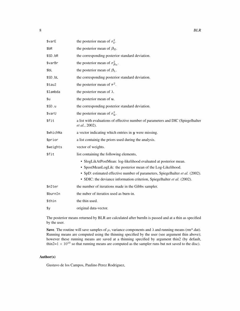
A list with posterior means, posterior standard deviations, and the parameters used to fit the model:

$yHat the posterior mean of 1µ+XFβF +XRβR +XLβL +Zu+ ε.

$SD.yHat the corresponding posterior standard deviation.

$mu the posterior mean of the intercept.

8 BLR

$varE the posterior mean of σ2ε.

$bR the posterior mean of βR.

$SD.bR the corresponding posterior standard deviation.

$varBr the posterior mean of σ2βR

.

$bL the posterior mean of βL.

$SD.bL the corresponding posterior standard deviation.

$tau2 the posterior mean of τ 2.

$lambda the posterior mean of λ.

$u the posterior mean of u.

$SD.u the corresponding posterior standard deviation.

$varU the posterior mean of σ2u.

$fit a list with evaluations of effective number of parameters and DIC (Spiegelhalteret al., 2002).

$whichNa a vector indicating which entries in y were missing.

$prior a list containig the priors used during the analysis.

$weights vector of weights.

$fit list containing the following elements,

• $logLikAtPostMean: log-likelihood evaluated at posterior mean.

• $postMeanLogLik: the posterior mean of the Log-Likelihood.

• $pD: estimated effective number of parameters, Spiegelhalter et al. (2002).

• $DIC: the deviance information criterion, Spiegelhalter et al. (2002).

$nIter the number of iterations made in the Gibbs sampler.

$burnIn the nuber of iteratios used as burn-in.

$thin the thin used.

$y original data-vector.

The posterior means returned by BLR are calculated after burnIn is passed and at a thin as specifiedby the user.

Save. The routine will save samples of µ, variance components and λ and running means (rm*.dat).Running means are computed using the thinning specified by the user (see argument thin above);however these running means are saved at a thinning specified by argument thin2 (by default,thin2=1× 1010 so that running means are computed as the sampler runs but not saved to the disc).

Author(s)

Gustavo de los Campos, Paulino Perez Rodriguez,

BLR 9

References

de los Campos G., H. Naya, D. Gianola, J. Crossa, A. Legarra, E. Manfredi, K. Weigel and J. Cotes.2009. Predicting Quantitative Traits with Regression Models for Dense Molecular Markers andPedigree. Genetics 182: 375-385.

Park T. and G. Casella. 2008. The Bayesian LASSO. Journal of the American Statistical Associa-tion 103: 681-686.

Spiegelhalter, D.J., N.G. Best, B.P. Carlin and A. van der Linde. 2002. Bayesian measures of modelcomplexity and fit (with discussion). Journal of the Royal Statistical Society, Series B (StatisticalMethodology) 64 (4): 583-639.

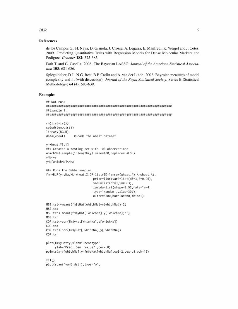
Examples

## Not run:##########################################################################Example 1:########################################################################

rm(list=ls())setwd(tempdir())library(BGLR)data(wheat) #Loads the wheat dataset

y=wheat.Y[,1]### Creates a testing set with 100 observationswhichNa<-sample(1:length(y),size=100,replace=FALSE)yNa<-yyNa[whichNa]<-NA

### Runs the Gibbs samplerfm<-BLR(y=yNa,XL=wheat.X,GF=list(ID=1:nrow(wheat.A),A=wheat.A),

prior=list(varE=list(df=3,S=0.25),varU=list(df=3,S=0.63),lambda=list(shape=0.52,rate=1e-4,type='random',value=30)),nIter=5500,burnIn=500,thin=1)

MSE.tst<-mean((fm$yHat[whichNa]-y[whichNa])^2)MSE.tstMSE.trn<-mean((fm$yHat[-whichNa]-y[-whichNa])^2)MSE.trnCOR.tst<-cor(fm$yHat[whichNa],y[whichNa])COR.tstCOR.trn<-cor(fm$yHat[-whichNa],y[-whichNa])COR.trn

plot(fm$yHat~y,xlab="Phenotype",ylab="Pred. Gen. Value" ,cex=.8)

points(x=y[whichNa],y=fm$yHat[whichNa],col=2,cex=.8,pch=19)

x11()plot(scan('varE.dat'),type="o",

10 BLR

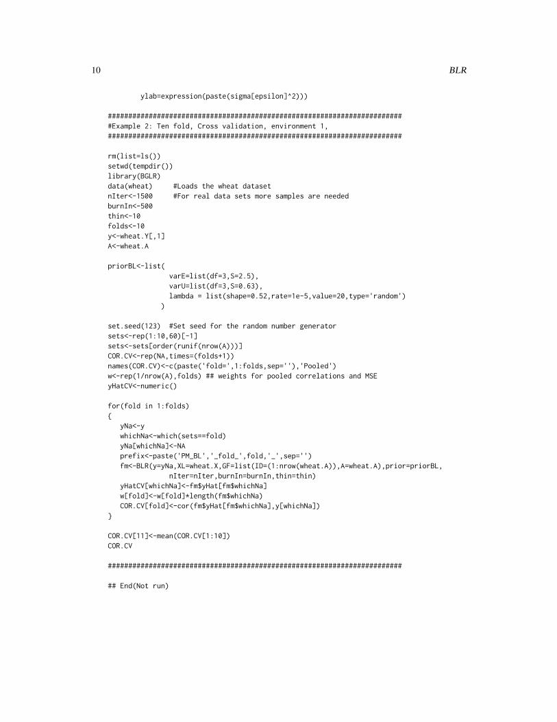
ylab=expression(paste(sigma[epsilon]^2)))

#########################################################################Example 2: Ten fold, Cross validation, environment 1,########################################################################

rm(list=ls())setwd(tempdir())library(BGLR)data(wheat) #Loads the wheat datasetnIter<-1500 #For real data sets more samples are neededburnIn<-500thin<-10folds<-10y<-wheat.Y[,1]A<-wheat.A

priorBL<-list(varE=list(df=3,S=2.5),varU=list(df=3,S=0.63),lambda = list(shape=0.52,rate=1e-5,value=20,type='random')

)

set.seed(123) #Set seed for the random number generatorsets<-rep(1:10,60)[-1]sets<-sets[order(runif(nrow(A)))]COR.CV<-rep(NA,times=(folds+1))names(COR.CV)<-c(paste('fold=',1:folds,sep=''),'Pooled')w<-rep(1/nrow(A),folds) ## weights for pooled correlations and MSEyHatCV<-numeric()

for(fold in 1:folds){

yNa<-ywhichNa<-which(sets==fold)yNa[whichNa]<-NAprefix<-paste('PM_BL','_fold_',fold,'_',sep='')fm<-BLR(y=yNa,XL=wheat.X,GF=list(ID=(1:nrow(wheat.A)),A=wheat.A),prior=priorBL,

nIter=nIter,burnIn=burnIn,thin=thin)yHatCV[whichNa]<-fm$yHat[fm$whichNa]w[fold]<-w[fold]*length(fm$whichNa)COR.CV[fold]<-cor(fm$yHat[fm$whichNa],y[whichNa])

}

COR.CV[11]<-mean(COR.CV[1:10])COR.CV

########################################################################

## End(Not run)

getVariances 11

getVariances getVariances

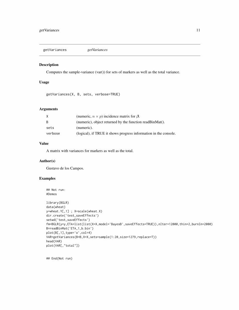
Description

Computes the sample-variance (var()) for sets of markers as well as the total variance.

Usage

getVariances(X, B, sets, verbose=TRUE)

Arguments

X (numeric, n× p) incidence matrix for β.B (numeric), object returned by the function readBinMat().sets (numeric).verbose (logical), if TRUE it shows progress information in the console.

Value

A matrix with variances for markers as well as the total.

Author(s)

Gustavo de los Campos.

Examples

## Not run:#Demos

library(BGLR)data(wheat)y=wheat.Y[,1] ; X=scale(wheat.X)dir.create('test_saveEffects')setwd('test_saveEffects')fm=BGLR(y=y,ETA=list(list(X=X,model='BayesB',saveEffects=TRUE)),nIter=12000,thin=2,burnIn=2000)B=readBinMat('ETA_1_b.bin')plot(B[,1],type='o',col=4)VAR=getVariances(B=B,X=X,sets=sample(1:20,size=1279,replace=T))head(VAR)plot(VAR[,"total"])

## End(Not run)

12 mice.A

mice mice dataset

Description

The mice data comes from an experiment carried out to detect and locate QTLs for complex traits ina mice population (Valdar et al. 2006a; 2006b). This data has already been analyzed for comparinggenome-assisted genetic evaluation methods (Legarra et al. 2008). The data file consists of 1814individuals, each genotyped for 10,346 polymorphic markers. The trait here here is body massindex (BMI), and additional information about body weight, season, month and day.

Usage

data(mice)

Format

Matrix mice.A contains the pedigree. The matrix mice.X contains the markes information andmice.pheno contains phenotypical information.

References

Legarra A., Robert-Granie, E. Manfredi, and J. M. Elsen, 2008 Performance of genomic selectionin mice. Genetics 180:611-618.

Valdar, W., L. C. Solberg, D. Gauguier, S. Burnett, P. Klenerman et al., 2006a Genome-wide geneticassociation of complex traits in heterogeneous stock mice. Nat. Genet. 38:879-887.

Valdar, W., L. C. Solberg, D. Gauguier, W. O. Cookson, J. N. P. Rawlis et al., 2006b Genetic andenvironmental effects on complex traits in mice. Genetics, 174:959-984.

mice.A Pedigree info for the mice dataset

Description

Is a numerator relationship matrix (1814 x 1814) computed from a pedigree that traced back manygenerations.

References

de los Campos G., H. Naya, D. Gianola, J. Crossa, A. Legarra, E. Manfredi, K. Weigel and J. Cotes.2009. Predicting Quantitative Traits with Regression Models for Dense Molecular Markers andPedigree. Genetics 182: 375-385.

mice.pheno 13

mice.pheno Phenotypical data for the mice dataset

Description

A data frame with pheotypical information related to diabetes. The data frame has several columns:SUBJECT.NAME, PROJECT.NAME, PHENOTYPE.NAME, Obesity.BMI, Obesity.BodyLength,Date.Month, Date.Year, Date.Season,cDate.StudyStartSeconds, Date.Hour, Date.StudyDay, GEN-DER, EndNormalBW, CoatColour, CageDensity, Litter, cage.

The phenotypes are described in http://gscan.well.ox.ac.uk.

mice.X Molecular markers

Description

Is a matrix ( 1814 x 10346) with SNP markers.

plot.BGLR Plots for BGLR Analysis

Description

Plots observed vs predicted values for objects of class BGLR.

Usage

## S3 method for class 'BGLR'plot(x, ...)

Arguments

x An object of class BGLR.

... Further arguments passed to or from other methods.

Author(s)

Gustavo de los Campos, Paulino Perez Rodriguez,

See Also

BGLR.

14 predict.BGLR

Examples

## Not run:

setwd(tempdir())library(BGLR)data(wheat)out=BLR(y=wheat.Y[,1],XL=wheat.X)plot(out)

## End(Not run)

predict.BGLR Model Predictions

Description

extracts predictions from the results of BGLR function.

Usage

## S3 method for class 'BGLR'predict(object, newdata, ...)

Arguments

object An object of class BGLR.

newdata Currently not supported, for new data you should assing missing value indicator(NAs) to the corresponding entries in the response vector (y).

... Further arguments passed to or from other methods.

Author(s)

Gustavo de los Campos, Paulino Perez Rodriguez,

See Also

BGLR.

readBinMat 15

Examples

## Not run:

setwd(tempdir())library(BGLR)data(wheat)out=BLR(y=wheat.Y[,1],XL=wheat.X)predict(out)

## End(Not run)

readBinMat readBinMat

Description

Function to read effects saved by BGLR when ETA[[j]]$saveEffects=TRUE.

Usage

readBinMat(filename,byrow=TRUE)

Arguments

filename (string), the name of the file to be read.

byrow (logical), if TRUE the matrix is created by filling its corresponding elements byrows.

Value

A matrix with samples of regression coefficients.

Author(s)

Gustavo de los Campos.

Examples

## Not run:#Demos

library(BGLR)data(wheat)

16 read_bed

y=wheat.Y[,1] ; X=scale(wheat.X)dir.create('test_saveEffects')setwd('test_saveEffects')fm=BGLR(y=y,ETA=list(list(X=X,model='BayesB',saveEffects=TRUE)),nIter=12000,thin=2,burnIn=2000)B=readBinMat('ETA_1_b.bin')

## End(Not run)

read_bed read_bed

Description

This function reads genotype information stored in binary PED (BED) files used in plink. Thesefiles save space and time. The pedigree/phenotype information is stored in a separate file (*.fam)and the map information is stored in an extededed MAP file (*.bim) that contains information aboutthe allele names, which would otherwise be lost in the BED file. More details http://zzz.bwh.harvard.edu/plink/binary.shtml.

Usage

read_bed(bed_file,bim_file,fam_file,na.strings,verbose)

Arguments

bed_file binary file with genotype information.

bim_file text file with pedigree/phenotype information.

fam_file text file with extended map information.

na.strings missing value indicators, default=c("0","-9").

verbose logical, if true print hex dump of bed file.

Value

The routine will return a vector of dimension n*p (n=number of individuals, p=number of snps),with the snps(individuals) stacked, depending whether the BED file is in SNP-major or individual-major mode.

The vector contains integer codes:

Integer code Genotype0 00 Homozygote "1"/"1"1 01 Heterozygote2 10 Missing genotype3 11 Homozygote "2"/"2"

read_ped 17

Author(s)

Gustavo de los Campos, Paulino Perez Rodriguez,

Examples

## Not run:

library(BGLR)demo(read_bed)

## End(Not run)

read_ped read_ped

Description

This function reads genotype information stored in PED format used in plink.

Usage

read_ped(ped_file)

Arguments

ped_file ASCII file with genotype information.

Details

The PED file is a white-space (space or tab) delimited file: the first six columns are mandatory:

Family ID Individual ID Paternal ID Maternal ID Sex (1=male; 2=female; other=unknown) Pheno-type

The IDs are alphanumeric: the combination of family and individual ID should uniquely identify aperson. A PED file must have 1 and only 1 phenotype in the sixth column. The phenotype can beeither a quantitative trait or an affection status column.

Value

The routine will return a vector of dimension n*p (n=number of individuals, p=number of snps),with the snps stacked.

The vector contains integer codes:

Integer code Genotype0 00 Homozygote "1"/"1"

18 residuals.BGLR

1 01 Heterozygote2 10 Missing genotype3 11 Homozygote "2"/"2"

Author(s)

Gustavo de los Campos, Paulino Perez Rodriguez,

Examples

## Not run:

library(BGLR)demo(read_ped)

## End(Not run)

residuals.BGLR Extracts models residuals

Description

extracts model residuals from objects returned by BGLR function.

Usage

## S3 method for class 'BGLR'residuals(object, ...)

Arguments

object An object of class BGLR.

... Further arguments passed to or from other methods.

Author(s)

Gustavo de los Campos, Paulino Perez Rodriguez,

See Also

BGLR.

summary.BGLR 19

Examples

## Not run:

setwd(tempdir())library(BGLR)data(wheat)out=BLR(y=wheat.Y[,1],XL=wheat.X)residuals(out)

## End(Not run)

summary.BGLR summary for BGLR fitted models

Description

Gives a summary for a fitted model using BGLR function.

Usage

## S3 method for class 'BGLR'summary(object, ...)

Arguments

object An object of class BGLR.

... Further arguments passed to or from other methods.

Author(s)

Gustavo de los Campos, Paulino Perez Rodriguez,

See Also

BGLR.

Examples

## Not run:

setwd(tempdir())library(BGLR)data(wheat)out=BLR(y=wheat.Y[,1],XL=wheat.X)summary(out)

20 wheat

## End(Not run)

wheat wheat dataset

Description

Information from a collection of 599 historical CIMMYT wheat lines. The wheat data set is fromCIMMYT’s Global Wheat Program. Historically, this program has conducted numerous interna-tional trials across a wide variety of wheat-producing environments. The environments representedin these trials were grouped into four basic target sets of environments comprising four main agro-climatic regions previously defined and widely used by CIMMYT’s Global Wheat Breeding Pro-gram. The phenotypic trait considered here was the average grain yield (GY) of the 599 wheat linesevaluated in each of these four mega-environments.

A pedigree tracing back many generations was available, and the Browse application of the Interna-tional Crop Information System (ICIS), as described in http://repository.cimmyt.org/xmlui/bitstream/handle/10883/3488/72673.pdf (McLaren et al. 2000, 2005) was used for derivingthe relationship matrix A among the 599 lines; it accounts for selection and inbreeding.

Wheat lines were recently genotyped using 1447 Diversity Array Technology (DArT) generated byTriticarte Pty. Ltd. (Canberra, Australia; http://www.triticarte.com.au). The DArT markersmay take on two values, denoted by their presence or absence. Markers with a minor allele fre-quency lower than 0.05 were removed, and missing genotypes were imputed with samples fromthe marginal distribution of marker genotypes, that is, xij = Bernoulli(p̂j), where p̂j is the es-timated allele frequency computed from the non-missing genotypes. The number of DArT MMsafter edition was 1279.

Usage

data(wheat)

Format

Matrix Y contains the average grain yield, column 1: Grain yield for environment 1 and so on.The matrix A contains additive relationship computed from the pedigree and matrix X contains themarkers information.

Source

International Maize and Wheat Improvement Center (CIMMYT), Mexico.

wheat.A 21

References

McLaren, C. G., L. Ramos, C. Lopez, and W. Eusebio. 2000. “Applications of the geneaologymanegment system.” In International Crop Information System. Technical Development Manual,version VI, edited by McLaren, C. G., J.W. White and P.N. Fox. pp. 5.8-5.13. CIMMyT, Mexico:CIMMyT and IRRI.

McLaren, C. G., R. Bruskiewich, A.M. Portugal, and A.B. Cosico. 2005. The International RiceInformation System. A platform for meta-analysis of rice crop data. Plant Physiology 139: 637-642.

wheat.A Pedigree info for the wheat dataset

Description

Is a numerator relationship matrix (599 x 599) computed from a pedigree that traced back manygenerations. This relationship matrix was derived using the Browse application of the Interna-tional Crop Information System (ICIS), as described in http://repository.cimmyt.org/xmlui/bitstream/handle/10883/3488/72673.pdf (McLaren et al. 2000, 2005).

Source

International Maize and Wheat Improvement Center (CIMMYT), Mexico.

References

McLaren, C. G., L. Ramos, C. Lopez, and W. Eusebio. 2000. “Applications of the geneaologymanegment system.” In International Crop Information System. Technical Development Manual,version VI, edited by McLaren, C. G., J.W. White and P.N. Fox. pp. 5.8-5.13. CIMMyT, Mexico:CIMMyT and IRRI.

McLaren, C. G., R. Bruskiewich, A.M. Portugal, and A.B. Cosico. 2005. The International RiceInformation System. A platform for meta-analysis of rice crop data. Plant Physiology 139: 637-642.

wheat.sets Sets for cross validation (CV)

Description

Is a vector (599 x 1) that assigns observations to 10 disjoint sets; the assignment was generated atrandom. This is used later to conduct a 10-fold CV.

Source

International Maize and Wheat Improvement Center (CIMMYT), Mexico.

22 write_bed

wheat.X Molecular markers

Description

Is a matrix (599 x 1279) with DArT genotypes; data are from pure lines and genotypes were codedas 0/1 denoting the absence/presence of the DArT. Markers with a minor allele frequency lowerthan 0.05 were removed, and missing genotypes were imputed with samples from the marginaldistribution of marker genotypes, that is, xij = Bernoulli(p̂j), where p̂j is the estimated allelefrequency computed from the non-missing genotypes. The number of DArT MMs after edition was1279.

Source

International Maize and Wheat Improvement Center (CIMMYT), Mexico.

wheat.Y Grain yield

Description

A matrix (599 x 4) containing the 2-yr average grain yield of each of these lines in each of the fourenvironments (phenotypes were standardized to a unit variance within each environment).

Source

International Maize and Wheat Improvement Center (CIMMYT), Mexico.

write_bed write_bed

Description

This function writes genotype information into a binary PED (BED) filed used in plink. For moredetails about this format see http://zzz.bwh.harvard.edu/plink/binary.shtml.

Usage

write_bed(x,n,p,bed_file)

write_bed 23

Arguments

n integer, number of individuals.

p integer, number of SNPs.

x integer vector that contains the genotypic information coded as 0,1,2 and 3 (seedetails below). The information must be in snp major order. The vector shouldbe of dimension n*p with the snps stacked.

bed_file output binary file with genotype information.

Details

The vector contains integer codes:

Integer code Genotype0 00 Homozygote "1"/"1"1 01 Heterozygote2 10 Missing genotype3 11 Homozygote "2"/"2"

Author(s)

Gustavo de los Campos, Paulino Perez Rodriguez,

Examples

## Not run:

library(BGLR)demo(write_bed)

## End(Not run)

Index

∗Topic datasetsmice, 12mice.A, 12mice.pheno, 13mice.X, 13wheat, 20wheat.A, 21wheat.sets, 21wheat.X, 22wheat.Y, 22

∗Topic modelsBGLR, 2BLR, 5getVariances, 11readBinMat, 15

∗Topic plotplot.BGLR, 13

∗Topic residualsresiduals.BGLR, 18

∗Topic summarysummary.BGLR, 19

BGLR, 2BLR, 5

getVariances, 11

mice, 12mice.A, 12mice.pheno, 13mice.X, 13

plot.BGLR, 13predict.BGLR, 14

read_bed, 16read_ped, 17readBinMat, 15residuals.BGLR, 18

summary.BGLR, 19

wheat, 20wheat.A, 21wheat.sets, 21wheat.X, 22wheat.Y, 22write_bed, 22

24