PA2B

Reproducible Research 2: Analyzing NOAA Events toMap and Rank Top US Weather Threats.

Marc Borowczak2015-05-12

Synopsys

In a reproducible way, and using R-Studio tools, this analysis script retrieves and process NOAA cataloguedweather events to extract most harmfull or damaging threats affecting the United States. The analysis willattempt to answer: “Where, How Often and What Type of Events constitute for each state his major threats?”.After documenting the tools, retrieval anc cleaning/reformatting of the data, an analysis is conducted toextract, rank the Top5 and display the major weather threats catalogued up to 2011. Four different categoriesrepresenting facets ot this threat affecting Fatalities, Injuries, Property Damages and Crop Damages, quantifythese threats as catalogued in the NOAA database as EVTYPE. The Top5 threats of each category areextrated for each US State, and their yearly rate is normalized and combined. Visualization is made easy thrumapping accross the US, for both relative impact and relative frequency. This is performed on a spectrumof time windows, ranging between 5 to 25 years span to discern trends, and presented side-by-side. Havingassessed cumulative risk impact and frequency by location, the last step of this analysis quantifies andcompares each US State side-by-side with their respective cumulated threat index, with most impactingindividual event types quantified and color coded. It is expected that this type of analysis will contribute inevent preparation, based on prior events occurence, impact, frequency and localization.

System and Platform documentation

Sys.info()[1:5] # system info but exclude login and user info

## sysname release## "Windows" "7 x64"## version nodename## "build 7601, Service Pack 1" "STALLION"## machine## "x86-64"

project<-'PA2' # create new projectif (!file.exists(project)){dir.create(project)}userdir<-getwd() # user-defined startup directory (Drive:/~/PA2/)projectdir<-paste(userdir,project,sep="/")setwd(projectdir) # work from the project directorydatadir<-"./data" ; if (!file.exists("data")) { dir.create("data") } # data will reside in subdir

Loadind libraries

library(dplyr) # provides data manipulating functions

#### Attaching package: 'dplyr'

1

#### The following object is masked from 'package:stats':#### filter#### The following objects are masked from 'package:base':#### intersect, setdiff, setequal, union

library(ggplot2) # for graphicslibrary(magrittr) # ceci n'est pas une pipelibrary(scales) # for scaling maps in ggplotlibrary(RCurl) # handles bzip2 files as well

## Loading required package: bitops

library(tidyr) # to tidy the data

#### Attaching package: 'tidyr'#### The following object is masked from 'package:magrittr':#### extract

library(ggmap) # for maps

#### Attaching package: 'ggmap'#### The following object is masked from 'package:magrittr':#### inset

library(maps)library(reshape2)sessionInfo() # to document platform

## R version 3.2.0 (2015-04-16)## Platform: x86_64-w64-mingw32/x64 (64-bit)## Running under: Windows 7 x64 (build 7601) Service Pack 1#### locale:## [1] LC_COLLATE=English_United States.1252## [2] LC_CTYPE=English_United States.1252## [3] LC_MONETARY=English_United States.1252## [4] LC_NUMERIC=C## [5] LC_TIME=English_United States.1252#### attached base packages:## [1] stats graphics grDevices utils datasets methods base

2

#### other attached packages:## [1] reshape2_1.4.1 maps_2.3-9 ggmap_2.4 tidyr_0.2.0## [5] RCurl_1.95-4.6 bitops_1.0-6 scales_0.2.4 magrittr_1.5## [9] ggplot2_1.0.1 dplyr_0.4.1#### loaded via a namespace (and not attached):## [1] Rcpp_0.11.5 knitr_1.10 MASS_7.3-40## [4] munsell_0.4.2 lattice_0.20-31 geosphere_1.3-13## [7] colorspace_1.2-6 rjson_0.2.15 jpeg_0.1-8## [10] stringr_0.6.2 plyr_1.8.2 tools_3.2.0## [13] parallel_3.2.0 grid_3.2.0 gtable_0.1.2## [16] png_0.1-7 DBI_0.3.1 htmltools_0.2.6## [19] yaml_2.1.13 assertthat_0.1 digest_0.6.8## [22] RJSONIO_1.3-0 mapproj_1.2-2 formatR_1.2## [25] evaluate_0.7 rmarkdown_0.5.1 sp_1.1-0## [28] RgoogleMaps_1.2.0.7 proto_0.3-10

Notice this markdown was developed on a Windows 64-bit platform with the english US locale. The projectresides in the PA1 subdirectory and data will reside in PA/data subdir. We document the libraries usedand the session info provides reproducibility on the documented R Studio Platform and the Windows 7 x64version.

It must noted that the download implemented here is using a non-secured link, i.e. with reduced confidencecompared to a secured https protocol. However, knittr will encounter an error when attempting to download abinary (.zip) file with an https.protocol. Changing to a non-secured http url and setting file.download=“wb”allows knittr to progress. This is strictly observed when knitting and the following error message is generated:

Error in download.file(url, dest = filename, mode = “wb”) : unsupported URL scheme

Note also that R studio can handle https on the same binary file without error.

Data Processing

Loading and pre-processing the data into activity data frame is automated with this R chunk and the datafileis copied in the /data subdirectory.

url <- "http://d396qusza40orc.cloudfront.net/repdata%2Fdata%2FStormData.csv.bz2"filename <- paste(datadir,strsplit(url,"%2F")[[1]][length(strsplit(url,"%2F")[[1]])],sep="/")download.file(url, dest=filename, mode="wb")filename <-(list.files(path=datadir,full.names=T,recursive=T)) # now holds the csv filenameStormData <- read.csv(filename,header=TRUE,stringsAsFactors=FALSE) # populate data frameunlink(filename) # remove the .bz2 filesetwd(userdir) # return to original work dir

We observe basic information and missing data NA as indicated with basic data.frame characteristics

str(StormData)

## 'data.frame': 902297 obs. of 37 variables:## $ STATE__ : num 1 1 1 1 1 1 1 1 1 1 ...## $ BGN_DATE : chr "4/18/1950 0:00:00" "4/18/1950 0:00:00" "2/20/1951 0:00:00" "6/8/1951 0:00:00" ...## $ BGN_TIME : chr "0130" "0145" "1600" "0900" ...

3

## $ TIME_ZONE : chr "CST" "CST" "CST" "CST" ...## $ COUNTY : num 97 3 57 89 43 77 9 123 125 57 ...## $ COUNTYNAME: chr "MOBILE" "BALDWIN" "FAYETTE" "MADISON" ...## $ STATE : chr "AL" "AL" "AL" "AL" ...## $ EVTYPE : chr "TORNADO" "TORNADO" "TORNADO" "TORNADO" ...## $ BGN_RANGE : num 0 0 0 0 0 0 0 0 0 0 ...## $ BGN_AZI : chr "" "" "" "" ...## $ BGN_LOCATI: chr "" "" "" "" ...## $ END_DATE : chr "" "" "" "" ...## $ END_TIME : chr "" "" "" "" ...## $ COUNTY_END: num 0 0 0 0 0 0 0 0 0 0 ...## $ COUNTYENDN: logi NA NA NA NA NA NA ...## $ END_RANGE : num 0 0 0 0 0 0 0 0 0 0 ...## $ END_AZI : chr "" "" "" "" ...## $ END_LOCATI: chr "" "" "" "" ...## $ LENGTH : num 14 2 0.1 0 0 1.5 1.5 0 3.3 2.3 ...## $ WIDTH : num 100 150 123 100 150 177 33 33 100 100 ...## $ F : int 3 2 2 2 2 2 2 1 3 3 ...## $ MAG : num 0 0 0 0 0 0 0 0 0 0 ...## $ FATALITIES: num 0 0 0 0 0 0 0 0 1 0 ...## $ INJURIES : num 15 0 2 2 2 6 1 0 14 0 ...## $ PROPDMG : num 25 2.5 25 2.5 2.5 2.5 2.5 2.5 25 25 ...## $ PROPDMGEXP: chr "K" "K" "K" "K" ...## $ CROPDMG : num 0 0 0 0 0 0 0 0 0 0 ...## $ CROPDMGEXP: chr "" "" "" "" ...## $ WFO : chr "" "" "" "" ...## $ STATEOFFIC: chr "" "" "" "" ...## $ ZONENAMES : chr "" "" "" "" ...## $ LATITUDE : num 3040 3042 3340 3458 3412 ...## $ LONGITUDE : num 8812 8755 8742 8626 8642 ...## $ LATITUDE_E: num 3051 0 0 0 0 ...## $ LONGITUDE_: num 8806 0 0 0 0 ...## $ REMARKS : chr "" "" "" "" ...## $ REFNUM : num 1 2 3 4 5 6 7 8 9 10 ...

summary(StormData)

## STATE__ BGN_DATE BGN_TIME TIME_ZONE## Min. : 1.0 Length:902297 Length:902297 Length:902297## 1st Qu.:19.0 Class :character Class :character Class :character## Median :30.0 Mode :character Mode :character Mode :character## Mean :31.2## 3rd Qu.:45.0## Max. :95.0#### COUNTY COUNTYNAME STATE EVTYPE## Min. : 0.0 Length:902297 Length:902297 Length:902297## 1st Qu.: 31.0 Class :character Class :character Class :character## Median : 75.0 Mode :character Mode :character Mode :character## Mean :100.6## 3rd Qu.:131.0## Max. :873.0#### BGN_RANGE BGN_AZI BGN_LOCATI

4

## Min. : 0.000 Length:902297 Length:902297## 1st Qu.: 0.000 Class :character Class :character## Median : 0.000 Mode :character Mode :character## Mean : 1.484## 3rd Qu.: 1.000## Max. :3749.000#### END_DATE END_TIME COUNTY_END COUNTYENDN## Length:902297 Length:902297 Min. :0 Mode:logical## Class :character Class :character 1st Qu.:0 NA's:902297## Mode :character Mode :character Median :0## Mean :0## 3rd Qu.:0## Max. :0#### END_RANGE END_AZI END_LOCATI## Min. : 0.0000 Length:902297 Length:902297## 1st Qu.: 0.0000 Class :character Class :character## Median : 0.0000 Mode :character Mode :character## Mean : 0.9862## 3rd Qu.: 0.0000## Max. :925.0000#### LENGTH WIDTH F MAG## Min. : 0.0000 Min. : 0.000 Min. :0.0 Min. : 0.0## 1st Qu.: 0.0000 1st Qu.: 0.000 1st Qu.:0.0 1st Qu.: 0.0## Median : 0.0000 Median : 0.000 Median :1.0 Median : 50.0## Mean : 0.2301 Mean : 7.503 Mean :0.9 Mean : 46.9## 3rd Qu.: 0.0000 3rd Qu.: 0.000 3rd Qu.:1.0 3rd Qu.: 75.0## Max. :2315.0000 Max. :4400.000 Max. :5.0 Max. :22000.0## NA's :843563## FATALITIES INJURIES PROPDMG## Min. : 0.0000 Min. : 0.0000 Min. : 0.00## 1st Qu.: 0.0000 1st Qu.: 0.0000 1st Qu.: 0.00## Median : 0.0000 Median : 0.0000 Median : 0.00## Mean : 0.0168 Mean : 0.1557 Mean : 12.06## 3rd Qu.: 0.0000 3rd Qu.: 0.0000 3rd Qu.: 0.50## Max. :583.0000 Max. :1700.0000 Max. :5000.00#### PROPDMGEXP CROPDMG CROPDMGEXP## Length:902297 Min. : 0.000 Length:902297## Class :character 1st Qu.: 0.000 Class :character## Mode :character Median : 0.000 Mode :character## Mean : 1.527## 3rd Qu.: 0.000## Max. :990.000#### WFO STATEOFFIC ZONENAMES LATITUDE## Length:902297 Length:902297 Length:902297 Min. : 0## Class :character Class :character Class :character 1st Qu.:2802## Mode :character Mode :character Mode :character Median :3540## Mean :2875## 3rd Qu.:4019## Max. :9706

5

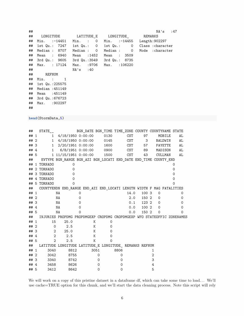
## NA's :47## LONGITUDE LATITUDE_E LONGITUDE_ REMARKS## Min. :-14451 Min. : 0 Min. :-14455 Length:902297## 1st Qu.: 7247 1st Qu.: 0 1st Qu.: 0 Class :character## Median : 8707 Median : 0 Median : 0 Mode :character## Mean : 6940 Mean :1452 Mean : 3509## 3rd Qu.: 9605 3rd Qu.:3549 3rd Qu.: 8735## Max. : 17124 Max. :9706 Max. :106220## NA's :40## REFNUM## Min. : 1## 1st Qu.:225575## Median :451149## Mean :451149## 3rd Qu.:676723## Max. :902297##

head(StormData,5)

## STATE__ BGN_DATE BGN_TIME TIME_ZONE COUNTY COUNTYNAME STATE## 1 1 4/18/1950 0:00:00 0130 CST 97 MOBILE AL## 2 1 4/18/1950 0:00:00 0145 CST 3 BALDWIN AL## 3 1 2/20/1951 0:00:00 1600 CST 57 FAYETTE AL## 4 1 6/8/1951 0:00:00 0900 CST 89 MADISON AL## 5 1 11/15/1951 0:00:00 1500 CST 43 CULLMAN AL## EVTYPE BGN_RANGE BGN_AZI BGN_LOCATI END_DATE END_TIME COUNTY_END## 1 TORNADO 0 0## 2 TORNADO 0 0## 3 TORNADO 0 0## 4 TORNADO 0 0## 5 TORNADO 0 0## COUNTYENDN END_RANGE END_AZI END_LOCATI LENGTH WIDTH F MAG FATALITIES## 1 NA 0 14.0 100 3 0 0## 2 NA 0 2.0 150 2 0 0## 3 NA 0 0.1 123 2 0 0## 4 NA 0 0.0 100 2 0 0## 5 NA 0 0.0 150 2 0 0## INJURIES PROPDMG PROPDMGEXP CROPDMG CROPDMGEXP WFO STATEOFFIC ZONENAMES## 1 15 25.0 K 0## 2 0 2.5 K 0## 3 2 25.0 K 0## 4 2 2.5 K 0## 5 2 2.5 K 0## LATITUDE LONGITUDE LATITUDE_E LONGITUDE_ REMARKS REFNUM## 1 3040 8812 3051 8806 1## 2 3042 8755 0 0 2## 3 3340 8742 0 0 3## 4 3458 8626 0 0 4## 5 3412 8642 0 0 5

We will work on a copy of this pristine dataset in a dataframe df, which can take some time to load. . . We’lluse cache=TRUE option for this chunk, and we’ll start the data cleaning process. Note this script will rely

6

heavily on the magrittr package, so analysts not familiar with this tool are refered to the vignette for furtherdetails.

df<-as.data.frame(StormData) # holds the df to analyzenames(df) %<>% tolowerdata(state.fips)

We convert the exponent prefix using generic Regex so we’ll be able to tally amounts of damages both forproperty and crop, and combine the result as a numeric value (multiplier)

df$propdmgexp %<>%gsub("[Kk]","3",.) %>%gsub("[Mm]","6",.) %>%gsub("[Hh]","2",.) %>%gsub("B","9",.) %>%gsub("[[:punct:]]","0",.) %>%sub("","0",.)df$propdmgexp<-10^as.numeric(df$propdmgexp)

df$cropdmgexp %<>%gsub("[Kk]","3",.) %>%gsub("[Mm]","6",.) %>%gsub("B","9",.) %>%gsub("[[:punct:]]","0",.) %>%sub("","0",.)df$cropdmgexp<-10^as.numeric(df$cropdmgexp)

We now only extract vectors we intend to process, combine the property and crop damages with theirrespective multiplier and retain only data entries that present a non-zero value in any of the 4 categories,then eliminate redundand exponents.

df %<>%select(bgn_date,bgn_time,evtype,fatalities,injuries,propdmg,propdmgexp,cropdmg,cropdmgexp,state__,state,county,countyname,longitude,latitude) %>%rename(date=bgn_date,time=bgn_time,state.FIBS=state__,county.FIBS=county,county=countyname) %>%mutate(propdmg=propdmg*propdmgexp,cropdmg=cropdmg*cropdmgexp) %>%filter(fatalities > 0 || injuries > 0|| propdmg>0 || cropdmg>0) %>%rename(propdamages=propdmg,cropdamages=cropdmg)df<-df[,-c(7,9)] # remove propdmgexp,cropdmgexp as they are redundant

The next step is to cleanup and format date and time

df$date %<>%gsub(" 0:00:00","",.) %>%as.Date("%m/%d/%Y")df$time %<>% strptime("%H%M") %>%format("%H:%M")

The next step is to cleanup event types for similar events based on shorthand, vocabulary or grammar asmany manual entries show obvious occurences (eg. evtype ending with s)

7

df$evtype %<>% toupper %>%gsub("WINDS","WIND",.) %>%gsub("STORMS","STORM",.) %>%gsub("FIRES","FIRE",.) %>%gsub("LANDSLIDES","LANDSLIDE",.) %>%gsub("FLD","FLOOD",.) %>%gsub("GLAZE","ICE",.) %>%gsub("CURRENTS","CURRENT",.) %>%replace(grepl("(?i)WIND",.,perl=TRUE),"WIND") %>%replace(grepl("(?i)SNOW",.,perl=TRUE),"SNOW") %>%replace(grepl("(?i)DUST",.,perl=TRUE),"DUST") %>%replace(grepl("(?i)HAIL",.,perl=TRUE),"HAIL") %>%replace(grepl("(?i)TIDE",.,perl=TRUE),"TIDE") %>%replace(grepl("(?i)FLOOD",.,perl=TRUE),"FLOOD") %>%replace(grepl("(?i)SURF",.,perl=TRUE),"SURF") %>%replace(grepl("(?i)ICE",.,perl=TRUE),"ICE") %>%replace(grepl("(?i)COLD",.,perl=TRUE),"COLD") %>%replace(grepl("(?i)HEAT",.,perl=TRUE),"HEAT") %>%replace(grepl("(?i)TROPICAL STORM",.,perl=TRUE),"TROPICAL STORM") %>%replace(grepl("(?i)FLOOD",.,perl=TRUE),"FLOOD") %>%replace(grepl("(?i)FOG",.,perl=TRUE),"FOG") %>%replace(grepl("(?i)SEAS",.,perl=TRUE),"HIGH SEAS") %>%replace(grepl("(?i)RAIN",.,perl=TRUE),"RAIN") %>%replace(grepl("(?i)MIX",.,perl=TRUE),"MIXED PRECIP") %>%replace(grepl("(?i)FUNNEL",.,perl=TRUE),"TORNADO") %>%replace(grepl("(?i)TORNADO",.,perl=TRUE),"TORNADO") %>%replace(grepl("(?i)TROPICAL",.,perl=TRUE),"TROPICAL") %>%replace(grepl("(?i)WINTER",.,perl=TRUE),"WINTER") %>%replace(grepl("(?i)HURRICANE",.,perl=TRUE),"HURRICANE") %>%replace(grepl("(?i)ICY",.,perl=TRUE),"ICE") %>%replace(grepl("(?i)MISHAP",.,perl=TRUE),"MARINE ACCIDENT") %>%replace(grepl("(?i)FIRE",.,perl=TRUE),"WILD FIRE")

As we intend to analyze both Impact (i.e. Magnitude) and Frequency, from the data retained in df, build ahigh impact (hi) and a high frequency (hf) datasets. These sets have same structure. Only difference is thatwe retain counts only for frequency, not magnitude of the events.

df %>%mutate(year=as.numeric(format(df$date,"%Y"))) %>%select(-date,-time) %>%group_by(state.FIBS,state,year,evtype,longitude,latitude) %>%summarize(total.fatalities=sum(fatalities),total.injuries=sum(injuries),total.propdamages=sum(propdamages),total.cropdamages=sum(cropdamages)) %>%arrange(desc(total.fatalities),desc(total.injuries),desc(total.propdamages),desc(total.cropdamages)) %>%as.data.frame -> hi

For the frequency dataset, start with a copy of hi and set all missing entries to 0, then substitutepositiveentries with 1 (count only)

hf<-hihf$total.fatalities[is.na(hf$total.fatalities)]<-0hf$total.injuries[is.na(hf$total.injuries)]<-0hf$total.propdamages[is.na(hf$total.propdamages)]<-0hf$total.cropdamages[is.na(hf$total.cropdamages)]<-0

8

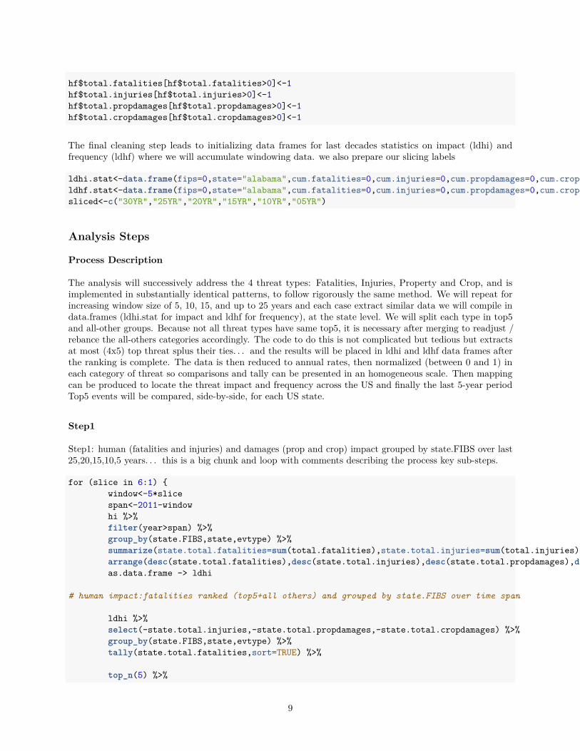
hf$total.fatalities[hf$total.fatalities>0]<-1hf$total.injuries[hf$total.injuries>0]<-1hf$total.propdamages[hf$total.propdamages>0]<-1hf$total.cropdamages[hf$total.cropdamages>0]<-1

The final cleaning step leads to initializing data frames for last decades statistics on impact (ldhi) andfrequency (ldhf) where we will accumulate windowing data. we also prepare our slicing labels

ldhi.stat<-data.frame(fips=0,state="alabama",cum.fatalities=0,cum.injuries=0,cum.propdamages=0,cum.cropdamages=0,ssa=0,region=0,division=0,abb="AL",polyname="alabama",span=0,slice=0) # inititialize data.frame for tallying statsldhf.stat<-data.frame(fips=0,state="alabama",cum.fatalities=0,cum.injuries=0,cum.propdamages=0,cum.cropdamages=0,ssa=0,region=0,division=0,abb="AL",polyname="alabama",span=0,slice=0) # inititialize data.frame for tallying statssliced<-c("30YR","25YR","20YR","15YR","10YR","05YR")

Analysis Steps

Process Description

The analysis will successively address the 4 threat types: Fatalities, Injuries, Property and Crop, and isimplemented in substantially identical patterns, to follow rigorously the same method. We will repeat forincreasing window size of 5, 10, 15, and up to 25 years and each case extract similar data we will compile indata.frames (ldhi.stat for impact and ldhf for frequency), at the state level. We will split each type in top5and all-other groups. Because not all threat types have same top5, it is necessary after merging to readjust /rebance the all-others categories accordingly. The code to do this is not complicated but tedious but extractsat most (4x5) top threat splus their ties. . . and the results will be placed in ldhi and ldhf data frames afterthe ranking is complete. The data is then reduced to annual rates, then normalized (between 0 and 1) ineach category of threat so comparisons and tally can be presented in an homogeneous scale. Then mappingcan be produced to locate the threat impact and frequency across the US and finally the last 5-year periodTop5 events will be compared, side-by-side, for each US state.

Step1

Step1: human (fatalities and injuries) and damages (prop and crop) impact grouped by state.FIBS over last25,20,15,10,5 years. . . this is a big chunk and loop with comments describing the process key sub-steps.

for (slice in 6:1) {window<-5*slicespan<-2011-windowhi %>%filter(year>span) %>%group_by(state.FIBS,state,evtype) %>%summarize(state.total.fatalities=sum(total.fatalities),state.total.injuries=sum(total.injuries),state.total.propdamages=sum(total.propdamages),state.total.cropdamages=sum(total.cropdamages)) %>%arrange(desc(state.total.fatalities),desc(state.total.injuries),desc(state.total.propdamages),desc(state.total.cropdamages)) %>%as.data.frame -> ldhi

# human impact:fatalities ranked (top5+all others) and grouped by state.FIBS over time span

ldhi %>%select(-state.total.injuries,-state.total.propdamages,-state.total.cropdamages) %>%group_by(state.FIBS,state,evtype) %>%tally(state.total.fatalities,sort=TRUE) %>%

top_n(5) %>%

9

as.data.frame -> ldhi.top5.fatalities

ldhi %>%select(-state.total.injuries,-state.total.propdamages,-state.total.cropdamages) %>%rename(n=state.total.fatalities) %>%setdiff(ldhi.top5.fatalities) %>%as.data.frame -> dftemp

# rename all non-top5 as "ALL OTHERS" and bind them back to ldhi.fatalities dataframe

dftemp$evtype<-"ALL OTHERS"dftemp %>%group_by(state.FIBS,state,evtype) %>%summarize(n=sum(n)) %>%as.data.frame %>%rbind(ldhi.top5.fatalities) %>%rename(state.fatalities=n) %>%arrange(state.FIBS,state,desc(state.fatalities)) %>%as.data.frame -> ldhi.fatalities

# human impact:injuries ranked (top5+all others) and grouped by state.FIBS over time span

ldhi %>%select(-state.total.fatalities,-state.total.propdamages,-state.total.cropdamages) %>%group_by(state.FIBS,state,evtype) %>%tally(state.total.injuries,sort=TRUE) %>%

top_n(5) %>%

as.data.frame -> ldhi.top5.injuries

ldhi %>%select(-state.total.fatalities,-state.total.propdamages,-state.total.cropdamages) %>%rename(n=state.total.injuries) %>%setdiff(ldhi.top5.injuries) %>%as.data.frame -> dftemp

# rename all non-top5 as "ALL OTHERS" and bind them back to ldhi.injuries dataframe

dftemp$evtype<-"ALL OTHERS"dftemp %>%group_by(state.FIBS,state,evtype) %>%summarize(n=sum(n)) %>%as.data.frame %>%rbind(ldhi.top5.injuries) %>%rename(state.injuries=n) %>%arrange(state.FIBS,state,desc(state.injuries)) %>%as.data.frame -> ldhi.injuries

# damages impact: props ranked (top5+all others) and grouped by state.FIBS over time span

ldhi %>%group_by(state.FIBS,state,evtype) %>%

10

tally(state.total.propdamages,sort=TRUE) %>%

top_n(5) %>%

as.data.frame -> ldhi.top5.propdamages

ldhi %>%select(-state.total.fatalities,-state.total.injuries,-state.total.cropdamages) %>%rename(n=state.total.propdamages) %>%setdiff(ldhi.top5.propdamages) %>%as.data.frame -> dftemp

# rename all non-top5 as "ALL OTHERS" and bind them back to ldhi.propdamages dataframe

dftemp$evtype<-"ALL OTHERS"dftemp %>%group_by(state.FIBS,state,evtype) %>%summarize(n=sum(n)) %>%as.data.frame %>%rbind(ldhi.top5.propdamages) %>%rename(state.propdamages=n) %>%arrange(state.FIBS,state,desc(state.propdamages)) %>%as.data.frame -> ldhi.propdamages

# damages impact: crops ranked (top5+all others) and grouped by state.FIBS over time span

ldhi %>%group_by(state.FIBS,state,evtype) %>%tally(state.total.cropdamages,sort=TRUE) %>%

top_n(5) %>%

as.data.frame -> ldhi.top5.cropdamages

ldhi %>%select(-state.total.fatalities,-state.total.injuries,-state.total.propdamages) %>%rename(n=state.total.cropdamages) %>%setdiff(ldhi.top5.cropdamages) %>%as.data.frame -> dftemp

# rename all non-top5 as "ALL OTHERS" and bind them back to ldhi.cropdamages dataframe

dftemp$evtype<-"ALL OTHERS"dftemp %>%group_by(state.FIBS,state,evtype) %>%summarize(n=sum(n)) %>%as.data.frame %>%rbind(ldhi.top5.cropdamages) %>%rename(state.cropdamages=n) %>%arrange(state.FIBS,state,desc(state.cropdamages)) %>%as.data.frame -> ldhi.cropdamages

# now merge back all categories together into the last decades high impact ranked dataframe ldhi.ranked

11

ldhi.fatalities %>%merge(ldhi.injuries, all=T) %>%merge(ldhi.propdamages, all=T) %>%merge(ldhi.cropdamages, all=T) %>%arrange(state.FIBS,state,desc(state.fatalities),desc(state.injuries),desc(state.propdamages),desc(state.cropdamages)) %>%as.data.frame -> ldhi.ranked

# after renaming the cumulative counts in each category, save the results in the high impact ldh dataframe

ldhi %>%rename(state.fatalities=state.total.fatalities,state.injuries=state.total.injuries,state.propdamages=state.total.propdamages,state.cropdamages=state.total.cropdamages) %>%as.data.frame -> ldhi

# since the top 5 in each categories do not necessarily overlap, we obtain some NAs after merging, which# we must replace with values in ldhi and compensate the "ALL OTHERS" counts for state.fatalities.# potentially we could endup with more than 20 aggregated top5, not counting the ties...# we will repeat the same process for all categories: fatalities, injuries, propdamages and cropdamages

subset(ldhi.ranked[,c(-5,-6,-7)],is.na(ldhi.ranked$state.fatalities)) %>% # retain only the missing activity steps data subset filter(is.na(state.fatalities)) %>%rename(missing.state.fatalities=state.fatalities) %>%merge(ldhi[,c(-5,-6,-7)], all=FALSE) %>%select(-missing.state.fatalities)-> ldhi.ranked.m # NAs have been substituted

# retain only the fatalities and tally the deductions for events that need readjusted in ldhi.ranked.agg

ldhi.ranked.nm<-subset(ldhi.ranked[,c(-5,-6,-7)],!is.na(ldhi.ranked$state.fatalities))

ldhi.ranked.m %>%mutate(evtype="ALL OTHERS") %>%group_by(state.FIBS,state,evtype) %>%summarize(state.fatalities=-sum(state.fatalities))-> ldhi.ranked.agg # and aggregated for deducting from "ALL OTHERS"

ldhi.ranked.nm %>%filter(evtype=="ALL OTHERS") %>%rename(target.state.fatalities=state.fatalities) %>%merge(ldhi.ranked.agg,all=FALSE) %>%mutate(state.fatalities=target.state.fatalities+state.fatalities) %>%select(-target.state.fatalities) %>% # we'll need to keep the records that show > 0 values after combiningmerge(ldhi.ranked.m,all=TRUE) %>%merge(ldhi.ranked.nm,all=TRUE) %>%group_by(state.FIBS,state,evtype) %>%summarize(state.fatalities=min(state.fatalities)) %>%arrange(state.FIBS,state,desc(state.fatalities)) %>%as.data.frame -> ldhi.ranked.fatalities

rm(ldhi.ranked.m,ldhi.ranked.nm,ldhi.ranked.agg) # cleanup

# must replace NAs with values in ldhi and compensate the "ALL OTHERS" counts for state.injuries

subset(ldhi.ranked[,c(-4,-6,-7)],is.na(ldhi.ranked$state.injuries)) %>% # retain only the missing activity steps data subsetfilter(is.na(state.fatalities)) %>%rename(missing.state.injuries=state.injuries) %>%merge(ldhi[,c(-4,-6,-7)], all=FALSE) %>%select(-missing.state.injuries)-> ldhi.ranked.m # NAs have been substituted

12

ldhi.ranked.nm<-subset(ldhi.ranked[,c(-4,-6,-7)],!is.na(ldhi.ranked$state.injuries))

ldhi.ranked.m %>%mutate(evtype="ALL OTHERS") %>%group_by(state.FIBS,state,evtype) %>%summarize(state.injuries=-sum(state.injuries))-> ldhi.ranked.agg # and aggregated for deducting from "ALL OTHERS"

ldhi.ranked.nm %>%filter(evtype=="ALL OTHERS") %>%rename(target.state.injuries=state.injuries) %>%merge(ldhi.ranked.agg,all=FALSE) %>%mutate(state.injuries=target.state.injuries+state.injuries) %>%select(-target.state.injuries) %>% # we'll need to keep the records that show > 0 values after combiningmerge(ldhi.ranked.m,all=TRUE) %>%merge(ldhi.ranked.nm,all=TRUE) %>%group_by(state.FIBS,state,evtype) %>%summarize(state.injuries=min(state.injuries)) %>%arrange(state.FIBS,state,desc(state.injuries)) %>%as.data.frame -> ldhi.ranked.injuries

rm(ldhi.ranked.m,ldhi.ranked.nm,ldhi.ranked.agg) # cleanup

# must replace NAs with values in ldhi and compensate the "ALL OTHERS" counts for state.propdamages

subset(ldhi.ranked[,c(-4,-5,-7)],is.na(ldhi.ranked$state.propdamages)) %>% # retain only the missing activity steps data subset filter(is.na(state.propdamages)) %>%rename(missing.state.propdamages=state.propdamages) %>%merge(ldhi[,c(-4,-5,-7)], all=FALSE) %>%select(-missing.state.propdamages)-> ldhi.ranked.m # NAs have been substituted

ldhi.ranked.nm<-subset(ldhi.ranked[,c(-4,-5,-7)],!is.na(ldhi.ranked$state.propdamages))

ldhi.ranked.m %>%mutate(evtype="ALL OTHERS") %>%group_by(state.FIBS,state,evtype) %>%summarize(state.propdamages=-sum(state.propdamages))-> ldhi.ranked.agg # and aggregated for deducting from "ALL OTHERS"

ldhi.ranked.nm %>%filter(evtype=="ALL OTHERS") %>%rename(target.state.propdamages=state.propdamages) %>%merge(ldhi.ranked.agg,all=FALSE) %>%mutate(state.propdamages=target.state.propdamages+state.propdamages) %>%select(-target.state.propdamages) %>% # we'll need to keep the records that show > 0 values after combiningmerge(ldhi.ranked.m,all=TRUE) %>%merge(ldhi.ranked.nm,all=TRUE) %>%group_by(state.FIBS,state,evtype) %>%summarize(state.propdamages=min(state.propdamages)) %>%arrange(state.FIBS,state,desc(state.propdamages)) %>%as.data.frame -> ldhi.ranked.propdamages

rm(ldhi.ranked.m,ldhi.ranked.nm,ldhi.ranked.agg) # cleanup

# must replace NAs with values in ldhi and compensate the "ALL OTHERS" counts for state.cropdamages

13

subset(ldhi.ranked[,c(-4,-5,-6)],is.na(ldhi.ranked$state.cropdamages)) %>% # retain only the missing activity steps data subsetfilter(is.na(state.fatalities)) %>%rename(missing.state.cropdamages=state.cropdamages) %>%merge(ldhi[,c(-4-5,-6)], all=FALSE) %>%select(-missing.state.cropdamages)-> ldhi.ranked.m # NAs have been substituted

ldhi.ranked.nm<-subset(ldhi.ranked[,c(-4,-5,-6)],!is.na(ldhi.ranked$state.cropdamages))

ldhi.ranked.m %>%mutate(evtype="ALL OTHERS") %>%group_by(state.FIBS,state,evtype) %>%summarize(state.cropdamages=-sum(state.cropdamages))-> ldhi.ranked.agg # and aggregated for deducting from "ALL OTHERS"

ldhi.ranked.nm %>%filter(evtype=="ALL OTHERS") %>%rename(target.state.cropdamages=state.cropdamages) %>%merge(ldhi.ranked.agg,all=FALSE) %>%mutate(state.cropdamages=target.state.cropdamages+state.cropdamages) %>%select(-target.state.cropdamages) %>% # we'll need to keep the records that show > 0 values after combiningmerge(ldhi.ranked.m,all=TRUE) %>%merge(ldhi.ranked.nm,all=TRUE) %>%group_by(state.FIBS,state,evtype) %>%summarize(state.cropdamages=min(state.cropdamages)) %>%arrange(state.FIBS,state,desc(state.cropdamages)) %>%as.data.frame -> ldhi.ranked.cropdamages

rm(ldhi.ranked.m,ldhi.ranked.nm,ldhi.ranked.agg) # cleanup

# we now aggregate back the adjusted ranked categories into ldhi# this appears complex but is only lengthy codewise due to my inexperience...

ldhi.ranked.fatalities %>%merge(ldhi.ranked.injuries,all=TRUE) %>%merge(ldhi.ranked.propdamages,all=TRUE) %>%merge(ldhi.ranked.cropdamages,all=TRUE) %>%filter(state.fatalities>0 || state.injuries>0 || state.propdamages>0 || state.cropdamages>0) %>% # now is the time to eliminate the 0 values we introducedarrange(state.FIBS,state,desc(state.fatalities),desc(state.injuries),desc(state.propdamages),desc(state.cropdamages)) %>%as.data.frame -> ldhi

# at this stage, ldhi contains for each state and each event category the last decades top events that had highest impact

rm(dftemp,ldhi.fatalities,ldhi.injuries,ldhi.propdamages,ldhi.cropdamages,ldhi.ranked.fatalities,ldhi.ranked.injuries,ldhi.ranked.propdamages,ldhi.ranked.cropdamages)

# Summarize by state.FIBS total casualities into ldhi.cum, which holds the data relative to the time slice#

ldhi %>% group_by(state.FIBS,state) %>%summarize(cum.fatalities=sum(state.fatalities),cum.injuries=sum(state.injuries),cum.propdamages=sum(state.propdamages),cum.cropdamages=sum(state.cropdamages)) %>%arrange(state,desc(cum.fatalities),desc(cum.injuries),desc(cum.propdamages),desc(cum.cropdamages)) %>%rename(fips=state.FIBS) %>%merge(state.fips,all=T) %>%as.data.frame -> ldhi.cum

# complete the records with the span (number of years we analyzed back in time) and the slice (a variable we loop on)

14

ldhi.cum$span<-2011-spanldhi.cum$slice<-slice

# populate the dataframe we'll use to analyze ldhi.stat

ldhi.stat <- rbind(ldhi.stat,ldhi.cum)

# now tackle the Threat Frequency Index. This is a repeat but addresses the counts of events rather than the impact

hf %>%filter(year>span) %>%group_by(state.FIBS,state,evtype) %>%summarize(state.total.fatalities=sum(total.fatalities),state.total.injuries=sum(total.injuries),state.total.propdamages=sum(total.propdamages),state.total.cropdamages=sum(total.cropdamages)) %>%arrange(desc(state.total.fatalities),desc(state.total.injuries),desc(state.total.propdamages),desc(state.total.cropdamages)) %>%as.data.frame -> ldhf

# human impact:fatalities ranked (top5+all others) and grouped by state.FIBS over time span

ldhf %>%select(-state.total.injuries,-state.total.propdamages,-state.total.cropdamages) %>%group_by(state.FIBS,state,evtype) %>%tally(state.total.fatalities,sort=TRUE) %>%

top_n(5) %>%

as.data.frame -> ldhf.top5.fatalities

ldhf %>%select(-state.total.injuries,-state.total.propdamages,-state.total.cropdamages) %>%rename(n=state.total.fatalities) %>%setdiff(ldhf.top5.fatalities) %>%as.data.frame -> dftempdftemp$evtype<-"ALL OTHERS"

dftemp %>%group_by(state.FIBS,state,evtype) %>%summarize(n=sum(n)) %>%as.data.frame %>%rbind(ldhf.top5.fatalities) %>%rename(state.fatalities=n) %>%arrange(state.FIBS,state,desc(state.fatalities)) %>%as.data.frame -> ldhf.fatalities

rm(ldhf.top5.fatalities)

# human impact:injuries ranked (top5+all others) and grouped by state.FIBS over time span

ldhf %>%select(-state.total.fatalities,-state.total.propdamages,-state.total.cropdamages) %>%group_by(state.FIBS,state,evtype) %>%tally(state.total.injuries,sort=TRUE) %>%

top_n(5) %>%

15

as.data.frame -> ldhf.top5.injuries

ldhf %>%select(-state.total.fatalities,-state.total.propdamages,-state.total.cropdamages) %>%rename(n=state.total.injuries) %>%setdiff(ldhf.top5.injuries) %>%as.data.frame -> dftemp

dftemp$evtype<-"ALL OTHERS"

dftemp %>%group_by(state.FIBS,state,evtype) %>%summarize(n=sum(n)) %>%as.data.frame %>%rbind(ldhf.top5.injuries) %>%rename(state.injuries=n) %>%arrange(state.FIBS,state,desc(state.injuries)) %>%as.data.frame -> ldhf.injuries

rm(ldhf.top5.injuries)

# damages impact: props ranked (top5+all others) and grouped by state.FIBS over time span

ldhf %>%group_by(state.FIBS,state,evtype) %>%tally(state.total.propdamages,sort=TRUE) %>%

top_n(5) %>%

as.data.frame -> ldhf.top5.propdamages

ldhf %>%select(-state.total.fatalities,-state.total.injuries,-state.total.cropdamages) %>%rename(n=state.total.propdamages) %>%setdiff(ldhf.top5.propdamages) %>%as.data.frame -> dftemp

dftemp$evtype<-"ALL OTHERS"

dftemp %>%group_by(state.FIBS,state,evtype) %>%summarize(n=sum(n)) %>%as.data.frame %>%rbind(ldhf.top5.propdamages) %>%rename(state.propdamages=n) %>%arrange(state.FIBS,state,desc(state.propdamages)) %>%as.data.frame -> ldhf.propdamages

rm(ldhf.top5.propdamages)

# damages impact: crops ranked (top5+all others) and grouped by state.FIBS over time span

ldhf %>%

16

group_by(state.FIBS,state,evtype) %>%tally(state.total.cropdamages,sort=TRUE) %>%

top_n(5) %>%

as.data.frame -> ldhf.top5.cropdamages

ldhf %>%select(-state.total.fatalities,-state.total.injuries,-state.total.propdamages) %>%rename(n=state.total.cropdamages) %>%setdiff(ldhf.top5.cropdamages) %>%as.data.frame -> dftemp

dftemp$evtype<-"ALL OTHERS"

dftemp %>%group_by(state.FIBS,state,evtype) %>%summarize(n=sum(n)) %>%as.data.frame %>%rbind(ldhf.top5.cropdamages) %>%rename(state.cropdamages=n) %>%arrange(state.FIBS,state,desc(state.cropdamages)) %>%as.data.frame -> ldhf.cropdamages

rm(ldhf.top5.cropdamages)

ldhf.fatalities %>%merge(ldhf.injuries, all=T) %>%merge(ldhf.propdamages, all=T) %>%merge(ldhf.cropdamages, all=T) %>%arrange(state.FIBS,state,desc(state.fatalities),desc(state.injuries),desc(state.propdamages),desc(state.cropdamages)) %>%as.data.frame -> ldhf.ranked

ldhf %>% rename(state.fatalities=state.total.fatalities,state.injuries=state.total.injuries,state.propdamages=state.total.propdamages,state.cropdamages=state.total.cropdamages) %>%as.data.frame -> ldhf

# must replace NAs with values in ldhf and compensate the "ALL OTHERS" counts for state.fatalities

subset(ldhf.ranked[,c(-5,-6,-7)],is.na(ldhf.ranked$state.fatalities)) %>% # retain only the missing activity steps data subset filter(is.na(state.fatalities)) %>%rename(missing.state.fatalities=state.fatalities) %>%merge(ldhf[,-c(5:7)], all=FALSE) %>%select(-missing.state.fatalities)-> ldhf.ranked.m # NAs have been substituted

ldhf.ranked.nm<-subset(ldhf.ranked[,c(-5,-6,-7)],!is.na(ldhf.ranked$state.fatalities))

ldhf.ranked.m %>%mutate(evtype="ALL OTHERS") %>%group_by(state.FIBS,state,evtype) %>%summarize(state.fatalities=-sum(state.fatalities))-> ldhf.ranked.agg # and aggregated for deducting from "ALL OTHERS"

ldhf.ranked.nm %>%filter(evtype=="ALL OTHERS") %>%rename(target.state.fatalities=state.fatalities) %>%

17

merge(ldhf.ranked.agg,all=FALSE) %>%mutate(state.fatalities=target.state.fatalities+state.fatalities) %>%select(-target.state.fatalities) %>% # we'll need to keep the records that show > 0 values after combiningmerge(ldhf.ranked.m,all=TRUE) %>%merge(ldhf.ranked.nm,all=TRUE) %>%group_by(state.FIBS,state,evtype) %>%summarize(state.fatalities=min(state.fatalities)) %>%arrange(state.FIBS,state,desc(state.fatalities)) %>%as.data.frame -> ldhf.ranked.fatalities

rm(ldhf.ranked.m,ldhf.ranked.nm,ldhf.ranked.agg) # cleanup

# must replace NAs with values in ldhf and compensate the "ALL OTHERS" counts for state.injuries

subset(ldhf.ranked[,c(-4,-6,-7)],is.na(ldhf.ranked$state.injuries)) %>% # retain only the missing activity steps data subsetfilter(is.na(state.fatalities)) %>%rename(missing.state.injuries=state.injuries) %>%merge(ldhf[,c(-4,-6,-7)], all=FALSE) %>%select(-missing.state.injuries)-> ldhf.ranked.m # NAs have been substituted

ldhf.ranked.nm<-subset(ldhf.ranked[,c(-4,-6,-7)],!is.na(ldhf.ranked$state.injuries))

ldhf.ranked.m %>%mutate(evtype="ALL OTHERS") %>%group_by(state.FIBS,state,evtype) %>%summarize(state.injuries=-sum(state.injuries))-> ldhf.ranked.agg # and aggregated for deducting from "ALL OTHERS"

ldhf.ranked.nm %>%filter(evtype=="ALL OTHERS") %>%rename(target.state.injuries=state.injuries) %>%merge(ldhf.ranked.agg,all=FALSE) %>%mutate(state.injuries=target.state.injuries+state.injuries) %>%select(-target.state.injuries) %>% # we'll need to keep the records that show > 0 values after combiningmerge(ldhf.ranked.m,all=TRUE) %>%merge(ldhf.ranked.nm,all=TRUE) %>%group_by(state.FIBS,state,evtype) %>%summarize(state.injuries=min(state.injuries)) %>%arrange(state.FIBS,state,desc(state.injuries)) %>%as.data.frame -> ldhf.ranked.injuries

rm(ldhf.ranked.m,ldhf.ranked.nm,ldhf.ranked.agg) # cleanup

# must replace NAs with values in ldhf and compensate the "ALL OTHERS" counts for state.propdamages

subset(ldhf.ranked[,c(-4,-5,-7)],is.na(ldhf.ranked$state.propdamages)) %>% # retain only the missing activity steps data subset filter(is.na(state.propdamages)) %>%rename(missing.state.propdamages=state.propdamages) %>%merge(ldhf[,c(-4,-5,-7)], all=FALSE) %>%select(-missing.state.propdamages)-> ldhf.ranked.m # NAs have been substituted

ldhf.ranked.nm<-subset(ldhf.ranked[,c(-4,-5,-7)],!is.na(ldhf.ranked$state.propdamages))

ldhf.ranked.m %>%mutate(evtype="ALL OTHERS") %>%group_by(state.FIBS,state,evtype) %>%

18

summarize(state.propdamages=-sum(state.propdamages))-> ldhf.ranked.agg # and aggregated for deducting from "ALL OTHERS"

ldhf.ranked.nm %>%filter(evtype=="ALL OTHERS") %>%rename(target.state.propdamages=state.propdamages) %>%merge(ldhf.ranked.agg,all=FALSE) %>%mutate(state.propdamages=target.state.propdamages+state.propdamages) %>%select(-target.state.propdamages) %>% # we'll need to keep the records that show > 0 values after combiningmerge(ldhf.ranked.m,all=TRUE) %>%merge(ldhf.ranked.nm,all=TRUE) %>%group_by(state.FIBS,state,evtype) %>%summarize(state.propdamages=min(state.propdamages)) %>%arrange(state.FIBS,state,desc(state.propdamages)) %>%as.data.frame -> ldhf.ranked.propdamages

rm(ldhf.ranked.m,ldhf.ranked.nm,ldhf.ranked.agg) # cleanup

# must replace NAs with values in ldhf and compensate the "ALL OTHERS" counts for state.cropdamages

subset(ldhf.ranked[,c(-4,-5,-6)],is.na(ldhf.ranked$state.cropdamages)) %>% # retain only the missing activity steps data subsetfilter(is.na(state.fatalities)) %>%rename(missing.state.cropdamages=state.cropdamages) %>%merge(ldhf[,c(-4-5,-6)], all=FALSE) %>%select(-missing.state.cropdamages)-> ldhf.ranked.m # NAs have been substituted

ldhf.ranked.nm<-subset(ldhf.ranked[,c(-4,-5,-6)],!is.na(ldhf.ranked$state.cropdamages))

ldhf.ranked.m %>%mutate(evtype="ALL OTHERS") %>%group_by(state.FIBS,state,evtype) %>%summarize(state.cropdamages=-sum(state.cropdamages))-> ldhf.ranked.agg # and aggregated for deducting from "ALL OTHERS"

ldhf.ranked.nm %>%filter(evtype=="ALL OTHERS") %>%rename(target.state.cropdamages=state.cropdamages) %>%merge(ldhf.ranked.agg,all=FALSE) %>%mutate(state.cropdamages=target.state.cropdamages+state.cropdamages) %>%select(-target.state.cropdamages) %>% # we'll need to keep the records that show > 0 values after combiningmerge(ldhf.ranked.m,all=TRUE) %>%merge(ldhf.ranked.nm,all=TRUE) %>%group_by(state.FIBS,state,evtype) %>%summarize(state.cropdamages=min(state.cropdamages)) %>%arrange(state.FIBS,state,desc(state.cropdamages)) %>%as.data.frame -> ldhf.ranked.cropdamages

rm(ldhf.ranked.m,ldhf.ranked.nm,ldhf.ranked.agg) # cleanup

ldhf.ranked.fatalities %>%merge(ldhf.ranked.injuries,all=TRUE) %>%merge(ldhf.ranked.propdamages,all=TRUE) %>%merge(ldhf.ranked.cropdamages,all=TRUE) %>%filter(state.fatalities>0 || state.injuries>0 || state.propdamages>0 || state.cropdamages>0) %>% # now is the time to eliminate the 0 values we introducedarrange(state.FIBS,state,desc(state.fatalities),desc(state.injuries),desc(state.propdamages),desc(state.cropdamages)) %>%as.data.frame -> ldhf

19

rm(dftemp,ldhf.fatalities,ldhf.injuries,ldhf.propdamages,ldhf.cropdamages,ldhf.ranked.fatalities,ldhf.ranked.injuries,ldhf.ranked.propdamages,ldhf.ranked.cropdamages)

# Summarize by state.FIBS total casualities

ldhf %>% group_by(state.FIBS,state) %>%summarize(cum.fatalities=sum(state.fatalities),cum.injuries=sum(state.injuries),cum.propdamages=sum(state.propdamages),cum.cropdamages=sum(state.cropdamages)) %>%arrange(state,desc(cum.fatalities),desc(cum.injuries),desc(cum.propdamages),desc(cum.cropdamages)) %>%rename(fips=state.FIBS) %>%merge(state.fips,all=T) %>%as.data.frame -> ldhf.cum

ldhf.cum$span<-2011-spanldhf.cum$slice<-slice

ldhf.stat <- rbind(ldhf.stat,ldhf.cum)}

## Selecting by n## Selecting by n## Selecting by n## Selecting by n## Selecting by n## Selecting by n## Selecting by n## Selecting by n## Selecting by n## Selecting by n## Selecting by n## Selecting by n## Selecting by n## Selecting by n## Selecting by n## Selecting by n## Selecting by n## Selecting by n## Selecting by n## Selecting by n## Selecting by n## Selecting by n## Selecting by n## Selecting by n## Selecting by n## Selecting by n## Selecting by n## Selecting by n## Selecting by n## Selecting by n## Selecting by n## Selecting by n## Selecting by n## Selecting by n## Selecting by n

20

## Selecting by n## Selecting by n## Selecting by n## Selecting by n## Selecting by n## Selecting by n## Selecting by n## Selecting by n## Selecting by n## Selecting by n## Selecting by n## Selecting by n## Selecting by n

Upon completion of the loop, we cleanup and strip the initial data row which served as template

rm(ldhi.cum,ldhi,ldhf.cum,ldhf)ldhi.stat<-ldhi.stat[-1,]ldhf.stat<-ldhf.stat[-1,]

We have now populated ldhi.stat and ldhf.stat with highest impact and highest frequency data over progres-sively smaller slicing periods. The next step will reduce this data so it can be mapped.

Step 2: Obtain Annual Rates

We start now the analysis to produce mappable data, starting with ldhi.stat, the impact dataframe, andwill repeat for the frequency data ldhf.stat in an identical way. First obtain the rate of impact by dividingcumulative values by time span (in years).

ldhi.stat %>%mutate(fatality.rate=cum.fatalities/ldhi.stat$span,injury.rate=cum.injuries/ldhi.stat$span,propdamage.rate=cum.propdamages/ldhi.stat$span,cropdamage.rate=cum.cropdamages/ldhi.stat$span) %>%as.data.frame ->ldhi

We continue by setting all missing values to 0 and populate the top vector with the max values, then normalizeby simply dividing each rate by the respective maximum value. . . and then produce the dataframe threati,in which we combine the localization data by merging with the state.fibs dataframe. This step is essential asmapping requires full name of the states, while the original dataset only provided the abbreviated statesnames.

It should be noted that to render AK and HI in this map requires additional work, using probably as bestcandidate a Chropleths approach as described in Vignette. We will leave it as a recommended future work toperform the adaptation.

ldhi$fatality.rate[is.na(ldhi$fatality.rate)]<-0ldhi$injury.rate[is.na(ldhi$injury.rate)]<-0ldhi$propdamage.rate[is.na(ldhi$propdamage.rate)]<-0ldhi$cropdamage.rate[is.na(ldhi$cropdamage.rate)]<-0

# determine maximum to normalize the data between 0 and 1 so we can compare between impact threat types

ldhi %>%select(fatality.rate,injury.rate,propdamage.rate,cropdamage.rate) %>%summarize(mfr=max(fatality.rate),mir=max(injury.rate),mpr=max(propdamage.rate),mcr=max(cropdamage.rate)) -> top

21

ldhi %>%mutate(Fatality=fatality.rate/top$mfr,Injury=injury.rate/top$mir,Property=propdamage.rate/top$mpr,Crop=cropdamage.rate/top$mcr) %>%merge(state.fips,all=F) %>%rename(state.abb=state,state=polyname) %>%subset(slice > 1) %>%as.data.frame -> threatithreati$slice<-as.factor(sliced[threati$slice])

At this stage, threati can be mapped, but we prefer the tidy data and use melt to reshape and set all missingvalues to 0, realizing the 30 year data will not bring significant departure to our observations

threati %>%droplevels %>%select(state,Fatality,Injury,Property,Crop,slice) %>%melt %>%

as.data.frame -> threatim

## Using state, slice as id variables

threatim$value[is.na(threatim$value)]<-0

We have completed the reduction of the data and threati and threatim (melted) contain the impact data formapping. The next step will be to display this observations.

Results 1: Impact Data Display

We now produce the facet maps for impact, in orange with a modified fill guide colorbar at bottom, using astemplate the chunk proposed in the ggplot documentation.

if (require(maps)) {states_map <- map_data("state")ggplot(threati, aes(map_id = state))+

geom_map(aes(fill = Fatality), map = states_map)+expand_limits(x = states_map$long, y = states_map$lat)

last_plot()+coord_map()ggplot(threatim, aes(map_id = state))+

geom_map(aes(fill = value), map = states_map)+expand_limits(x = states_map$long, y = states_map$lat)+theme(legend.position = "bottom")+guides(fill=guide_legend(title="Impact \nIndex"),guide_colorbar(barwidth = 10, barheight = .5))+scale_fill_gradient(low="white", high="orange")+facet_wrap(variable ~ slice)+labs(title="Fig.1 - US States Annual Weather-Dependent Aggregated Threat Impact Index 1986-2011 By Year Span\nBased on NOAA Reported Data")+xlab("Longitude")+ylab("Lattitude")

}

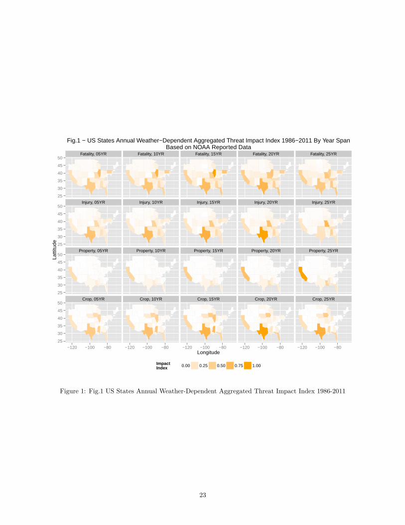
Fig.1 points out the localization in time and space the most impactful events and establish which states havebeen repeatedly observing them. Each category is normed, as an Index should, between 0 and 1. The higherthe Index, the higher the impact observed in the respective time span. Noticeable is Texas for recurrenceof impact events and concommitance of impact on almost all categories. Less severe impact is observed in

22

Fatality, 05YR Fatality, 10YR Fatality, 15YR Fatality, 20YR Fatality, 25YR

Injury, 05YR Injury, 10YR Injury, 15YR Injury, 20YR Injury, 25YR

Property, 05YR Property, 10YR Property, 15YR Property, 20YR Property, 25YR

Crop, 05YR Crop, 10YR Crop, 15YR Crop, 20YR Crop, 25YR

25

30

35

40

45

50

25

30

35

40

45

50

25

30

35

40

45

50

25

30

35

40

45

50

−120 −100 −80 −120 −100 −80 −120 −100 −80 −120 −100 −80 −120 −100 −80Longitude

Latti

tude

Impact Index 0.00 0.25 0.50 0.75 1.00

Fig.1 − US States Annual Weather−Dependent Aggregated Threat Impact Index 1986−2011 By Year SpanBased on NOAA Reported Data

Figure 1: Fig.1 US States Annual Weather-Dependent Aggregated Threat Impact Index 1986-2011

23

California and Illinoi. The Eastern/North-Eastern corridor sometimes reffered as “Tornado Alley” is quiteremarquable on this chart, and quite contrasted with the northern plains.

Let’s now look at the frequency of the same events. We prepare the frequency chart in totaly similar way togenerate threatf and threatfm

ldhf.stat %>%mutate(fatality.rate=cum.fatalities/ldhf.stat$span,injury.rate=cum.injuries/ldhf.stat$span,propdamage.rate=cum.propdamages/ldhf.stat$span,cropdamage.rate=cum.cropdamages/ldhf.stat$span) %>%as.data.frame ->ldhfldhf$fatality.rate[is.na(ldhf$fatality.rate)]<-0ldhf$injury.rate[is.na(ldhf$injury.rate)]<-0ldhf$propdamage.rate[is.na(ldhf$propdamage.rate)]<-0ldhf$cropdamage.rate[is.na(ldhf$cropdamage.rate)]<-0

ldhf %>%select(fatality.rate,injury.rate,propdamage.rate,cropdamage.rate) %>%summarize(mfr=max(fatality.rate),mir=max(injury.rate),mpr=max(propdamage.rate),mcr=max(cropdamage.rate)) -> top

ldhf %>%mutate(Fatality=fatality.rate/top$mfr,Injury=injury.rate/top$mir,Property=propdamage.rate/top$mpr,Crop=cropdamage.rate/top$mcr) %>%merge(.,state.fips,all=F) %>%rename(state.abb=state,state=polyname) %>%subset(slice >1) %>%as.data.frame -> threatfthreatf$slice<-as.factor(sliced[threatf$slice])

# we prefer tidy data and use melt to reshape and set all missing values to 0

threatf %>%droplevels %>%select(state,Fatality,Injury,Property,Crop,slice) %>%

melt %>%

as.data.frame -> threatfm

## Using state, slice as id variables

threatfm$value[is.na(threatfm$value)]<-0

We have completed the reduction of the data and threati and threatim contain the impact data for mapping.the next step will be to display these observations. The data frames threatf and threatfm contain thefrequency data for mapping.

Results 2: Frequency Data Display

We now produce the facet maps for frequency, in blue with a modified fill guide colorbar at bottom, using astemplate the chunk proposed in the ggplot vignette.

if (require(maps)) {states_map <- map_data("state")ggplot(threatf, aes(map_id = state))+

geom_map(aes(fill = Fatality), map = states_map)+

24

expand_limits(x = states_map$long, y = states_map$lat)last_plot()+coord_map()ggplot(threatfm, aes(map_id = state))+

geom_map(aes(fill = value), map = states_map)+expand_limits(x = states_map$long, y = states_map$lat)+theme(legend.position = "bottom")+guides(fill=guide_legend(title="Frequency\nIndex"),guide_colorbar(barwidth = 10, barheight = .5))+scale_fill_gradient(low="white", high="blue")+facet_wrap(variable ~ slice)+labs(title="Fig.2 - US States Annual Weather-Dependent Aggregated Threat Frequency Index 1986-2011\nBased on NOAA Reported Data")+xlab("Longitude")+ylab("Lattitude")

}

Fatality, 05YR Fatality, 10YR Fatality, 15YR Fatality, 20YR Fatality, 25YR

Injury, 05YR Injury, 10YR Injury, 15YR Injury, 20YR Injury, 25YR

Property, 05YR Property, 10YR Property, 15YR Property, 20YR Property, 25YR

Crop, 05YR Crop, 10YR Crop, 15YR Crop, 20YR Crop, 25YR

25

30

35

40

45

50

25

30

35

40

45

50

25

30

35

40

45

50

25

30

35

40

45

50

−120 −100 −80 −120 −100 −80 −120 −100 −80 −120 −100 −80 −120 −100 −80Longitude

Latti

tude

FrequencyIndex 0.00 0.25 0.50 0.75 1.00

Fig.2 − US States Annual Weather−Dependent Aggregated Threat Frequency Index 1986−2011Based on NOAA Reported Data

Figure 2: Fig.2 US States Annual Weather-Dependent Aggregated Threat Frequency Index 1986-2011

Fig.2 points out the localization in time and space of the most frequent events and establish which states havebeen repeatedly observing them. Each category is normed, as an Index should, between 0 and 1. The higherthe Index, the higher the frequency observed in the respective time span. Noticeable are Texas and generallythe South East of the US for recurrence of events and concommitance of frequency on almost all categories.Less frequent events are observed in California and in New Mexico. The Eastern/North-Eastern half of theUS is quite remarquable on this chart, and quite differentiated with the Pacific NorthWest, especially when

25

comparing crop and propertu damages. Overall, we do not observe drastic differences between impact andfrequency, also obviously a multiplier might be related to the local occupancy or activity. This is again leftfor further analysis.

Results 3: Threat Index 2006-2011 By US States

Having assessed Impact and Frequency, the nature of the threat will be now the focus of the latter part ofthe analysis. To this goal, we have chosen to perform the analysis on the data obtained from the last 5 years,assessing the categories leading to top5 threats in all 4 categories: Fatalities, Injuries, Property and Crop,and having a major impact (i.e. amongst top5 Impact).

We start with the top5 data frames we cumulated for each categories, add a type and calculate the normalizedindex similarly in each category, then bind all into the 4 threats data frames into the threats data frame.

ldhi.top5.fatalities$type<-"Fatality" # add a typeldhi.top5.injuries$type<-"Injury"ldhi.top5.propdamages$type<-"Property"ldhi.top5.cropdamages$type<-"Crop"

ldhi.top5.fatalities$n<-ldhi.top5.fatalities$n/(2011-span) # calculate annual rate over last 5 yearsldhi.top5.injuries$n<-ldhi.top5.injuries$n/(2011-span)ldhi.top5.propdamages$n<-ldhi.top5.propdamages$n/(2011-span)ldhi.top5.cropdamages$n<-ldhi.top5.cropdamages$n/(2011-span)

ldhi.top5.fatalities$n<-ldhi.top5.fatalities$n/max(ldhi.top5.fatalities$n) # normalize annual rate is indexldhi.top5.injuries$n<-ldhi.top5.injuries$n/max(ldhi.top5.injuries$n)ldhi.top5.propdamages$n<-ldhi.top5.propdamages$n/max(ldhi.top5.propdamages$n)ldhi.top5.cropdamages$n<-ldhi.top5.cropdamages$n/max(ldhi.top5.cropdamages$n)

ldhi.top5.fatalities %>% # now bind all normalized indexesrbind(ldhi.top5.injuries) %>%rbind(ldhi.top5.propdamages) %>%rbind(ldhi.top5.cropdamages) %>%as.data.frame -> threats

threats$evtype %<>% as.factorthreats$type %<>% as.factor

Let’s determine what evtype are listed and observe. . .

unique(threats$evtype)

## [1] TORNADO RIP CURRENT LIGHTNING WIND## [5] FLOOD HEAT BLIZZARD AVALANCHE## [9] DENSE SMOKE FROST/FREEZE HAIL ICE## [13] LANDSLIDE RAIN SNOW SURF## [17] TIDE WILD FIRE WINTER DROUGHT## [21] FOG TROPICAL DUST TSUNAMI## [25] HURRICANE VOLCANIC ASHFALL WATERSPOUT SEICHE## [29] SLEET## 29 Levels: AVALANCHE BLIZZARD DENSE SMOKE DROUGHT DUST FLOOD ... WINTER

We note it is time to reclassify by threats using Wikipedia’s classification as guide. . . so a colorscheme mightregroup visually similar threats. . .

26

threats$evtype %<>%gsub("WIND","1.0 WIND",.) %>%gsub("TORNADO","1.1 TORNADO",.) %>%gsub("HURRICANE","1.2 HURRICANE",.) %>%gsub("TROPICAL","1.4 TROPICAL STORM",.) %>%gsub("WATERSPOUT","1.5 WATERSPOUT",.) %>%gsub("DUST","1.6 DUST",.) %>%gsub("LIGHTNING","1.7 LIGHTNING",.) %>%gsub("WILD FIRE","1.8 WILD FIRE",.) %>%gsub("DENSE SMOKE","1.9 DENSE SMOKE",.) %>%gsub("HAIL","2.0 HAIL",.) %>%gsub("TSUNAMI","3.0 TSUNAMI",.) %>%gsub("FLOOD","3.1 FLOOD",.) %>%gsub("RAIN","3.2 RAIN",.) %>%gsub("TIDE","3.3 TIDE",.) %>%gsub("SURF","3.4 SURF",.) %>%gsub("SEICHE","3.5 SEICHE",.) %>%gsub("RIP CURRENT","3.6 RIP CURRENTS",.) %>%gsub("LANDSLIDE","3.7 LANDSLIDE",.) %>%gsub("WINTER","4.0 WINTER",.) %>%gsub("ICE","4.1 ICE",.) %>%gsub("BLIZZARD","4.2 BLIZZARD",.) %>%gsub("AVALANCHE","4.3 AVALANCHE",.) %>%gsub("SNOW","4.4 SNOW",.) %>%gsub("COLD","4.5 EXTREME COLD",.) %>%gsub("SLEET","4.6 SLEET",.) %>%gsub("FROST/FREEZE","4.7 FROST/FREEZE",.) %>%gsub("FOG","4.8 FOG",.) %>%gsub("DROUGHT","5.0 DROUGHT",.) %>%gsub("HEAT","5.1 HEAT",.) %>%gsub("VOLCANIC ASHFALL","5.2 VOLCANIC ASHFALL",.)

We observe the results of our reaarrangement with a significan reduction in event categories, but withimproved regrouping.

unique(threats$evtype)

## [1] "1.1 TORNADO" "3.6 RIP CURRENTS" "1.7 LIGHTNING"## [4] "1.0 WIND" "3.1 FLOOD" "5.1 HEAT"## [7] "4.2 BLIZZARD" "4.3 AVALANCHE" "1.9 DENSE SMOKE"## [10] "4.7 FROST/FREEZE" "2.0 HAIL" "4.1 ICE"## [13] "3.7 LANDSLIDE" "3.2 RAIN" "4.4 SNOW"## [16] "3.4 SURF" "3.3 TIDE" "1.8 WILD FIRE"## [19] "4.0 WINTER" "5.0 DROUGHT" "4.8 FOG"## [22] "1.4 TROPICAL STORM" "1.6 DUST" "3.0 TSUNAMI"## [25] "1.2 HURRICANE" "5.2 VOLCANIC ASHFALL" "1.5 WATERSPOUT"## [28] "3.5 SEICHE" "4.6 SLEET"

These are the threats we will now categorized by state and type, and perform some re-ordering so we maintainconsistency in our display charts.

27

threats %<>% select(-state.FIBS) %>%mutate (AVG.Index=n/4) %>% # to balance all unweightedgroup_by(state,type,evtype) %>%arrange(desc(AVG.Index)) %>%as.data.frame

threats$type<-factor(threats$type,levels(threats$type)[c(2,3,4,1)]) # reorder factor for display

We now have the combined top threats categorized by state and types, ready for plot, and will display abarplot to compare them side-by-side.

ggplot(threats, aes(x=state,y=AVG.Index,fill=evtype))+geom_bar(stat="identity")+guides(fill=guide_legend(title="Categorized Event Type",keywidth=2,keyheight=0.75))+theme(text = element_text(size=8) , axis.text.x = element_text(angle=90, vjust=1))+facet_wrap(~type , nrow=4, ncol=1)+labs(title="Fig.3 - US States Annual Weather-Dependent Averaged Threat Index 2006-2011 By US States\nBased on NOAA Reported Data")+xlab("Abbreviated United States")+ylab("Averaged Annual Threat Index")

Fatality

Injury

Property

Crop

0.00.10.20.30.4

0.00.10.20.30.4

0.00.10.20.30.4

0.00.10.20.30.4

AK

AL

AM

AN

AR

AS

AZ

CA

CO

CT

DC

DE

FL

GA

GM

GU HI

IA ID IL IN KS

KY

LA LC LE LH LM LO LS MA

MD

ME

MI

MN

MO

MS

MT

NC

ND

NE

NH

NJ

NM

NV

NY

OH

OK

OR

PA PH

PK

PR

PZ RI

SC

SD

TN

TX

UT

VA VI

VT

WA

WI

WV

WY

XX

Abbreviated United States

Ave

rage

d A

nnua

l Thr

eat I

ndex

1.2 HURRICANE

1.4 TROPICAL STORM

1.5 WATERSPOUT

1.6 DUST

1.7 LIGHTNING

1.8 WILD FIRE

1.9 DENSE SMOKE

2.0 HAIL

3.0 TSUNAMI

3.1 FLOOD

3.2 RAIN

3.3 TIDE

3.4 SURF

3.5 SEICHE

3.6 RIP CURRENTS

3.7 LANDSLIDE

4.0 WINTER

4.1 ICE

4.2 BLIZZARD

4.3 AVALANCHE

4.4 SNOW

4.6 SLEET

4.7 FROST/FREEZE

Fig.3 − US States Annual Weather−Dependent Averaged Threat Index 2006−2011 By US StatesBased on NOAA Reported Data

Figure 3: Fig.3 - US States Annual Weather-Dependent Averaged Threat Index 2006-2011

Fig.3 displays on an indexed categorized event type the comparative averaged annual threats for each USstate, aligned on the x-axis. It is important to not on this chart events associated with Iowa, Texax, Louisianaand Missouri, confirming some earlier discussed patterns.

Conclusions

This analysis is preliminary and the stategy employed is simply based on separating Impact, Frequencyassociated with an event occuring in a US State. . . Describing an event occurence can be addressed in termsof matching location, impact (or magnitude) and frequency patterns for categorized threats. Some trendsare apparent but the analysis on yearly index will improve with more data, as is predicted by the centrallimit theorem. However, determining trending data on this scale remains an open challenge, and the dataextracted from this analysis should only be used as a guide to help prepare for future occurences, shouldfuture weather patterns mimic prior observations.

28